Symbiosis Law School, NOIDA Bachelor of Arts & Bachelor of Laws ...
Upload
khangminh22Category
view
1download
0
UQ Engineering
Faculty of Engineering, Architecture and Information Technology
THE UNIVERSITY OF QUEENSLAND
Bachelor of Engineering Thesis
Investigating the Simulation Capabilities of ANSYS in
Modelling the Fundamental Antisymmetric Lamb Wave
Student Name: Jeffrey BARRETT
Course Code: MECH4500
Supervisor: Associate Professor Martin Veidt
Submission date: 22nd October 2018
A thesis submitted in partial fulfilment of the requirements of the Bachelor of Engineering
(Hons) degree in Mechanical and Aerospace Engineering

i
Acknowledgments Firstly, I would like to express my sincerest gratitude to Associate Professor Martin Veidt
for his continuing assistance throughout the project. Without his guidance, this thesis would not
have been possible. This project was an invaluable opportunity to develop my skills as a
professional engineer and I was very fortunate to have Martin as a mentor.
I would also like to thank my family for their amazing support throughout the entirety of
my university studies. Without the support of my mother and father, Nola and Ian, and my three
sisters, Amanda, Sally and Lisa, I would never have made it.
A special thanks to my friends who have been with me all the way through to the end.
Without the support from Tim, Andy, Dragan, Matt and Dan (to name a few), these past few
years would have been so much more difficult.
Finally, thank you Aísling for supporting me through the tough times. I could never express
how much your love and support has helped me, I couldn’t have done it without you.

ii
Abstract Structural health monitoring (SHM) is the continuous, real-time monitoring of the integrity
of a component, with the primary aim of detecting the onset of material damage [1, 2]. Some
SHM systems utilise networks of imbedded sensors to emit and receive Lamb waves, which are
elastic waves that propagate in thin structures [2]. When Lamb waves encounter structural
damage, the reflected waves contain information about the size, location and nature of the
damage [3]. Finite element method software packages such as ANSYS provide cost-effective
options for engineers to simulate Lamb wave propagation [2]. There is a strong motivation to
develop accurate and reliable numerical models of Lamb waves and their complex interactions
with structural damage. These models provide a valuable tool in the design of SHM systems.
The aim of the thesis was to investigate the simulation capabilities of ANSYS in modelling
the fundamental antisymmetric (A0) Lamb wave. The simulation results were to be compared
against analytical solutions to validate ANSYS as a numerical tool for modelling the A0 Lamb
wave. The investigation aimed to deliver a proven methodology for ANSYS simulation of the
A0 mode which could be used in future works relating to SHM system design.
A 2D model of an aluminium 2024-T6 plate was developed in ANSYS Explicit Dynamics.
The model was meshed using 4-node solid elements with characteristic lengths ranging from
0.15 – 1.50 mm. The A0 Lamb mode was activated by a 100 kHz sinusoidal tone burst,
modulated by a Hanning window. ANSYS was shown to accurately model the dispersive
properties of the A0 mode. The energy-distribution approach for time of arrival was the most
reliable method for calculating group velocity. ANSYS was found to accurately model group
velocity, with a minimum numerical error of only 0.15% The accuracy of the simulations
improved as mesh element length was reduced. The 2D Fast Fourier Transform was used to
calculate phase velocity of the incident wave pulse, with a numerical error of only 0.19%.
A three-dimensional model of the aluminium plate was developed in ANSYS using 8-
node brick elements. The simulation results showed good agreement with both the 2D and
analytical models, with an average error of 3.47% in A0 mode group velocity. The excitation
frequency was varied from 25 kHz – 400 kHz and group velocity results were used to develop
an experimental dispersion curve which showed excellent agreement with the analytical curve.
The mesh element length criterion was found to be noncritical for accurate ANSYS simulations.
A surface notch was developed in the 2D model. ANSYS accurately captured conversion
between the A0 and S0 modes due to interactions with the notch. Error in the reflected A0 and S0
modes was just 1.18% and 1.44% respectively. The amplitude of the reflected S0 mode
increased consistently with notch depth, while a mid-thickness notch caused the largest
amplitude of the A0 mode. A mid-thickness void was developed in the model. Only the A0 mode
was reflected from the damage, which was attributed to the through-thickness location of the
void. The amplitude of the reflected wave pulse increased consistently with void length between
1 – 5 mm, however no discernible trend was established for void lengths between 5 – 30 mm.
The capabilities of ANSYS in accurately modelling the A0 mode and its interactions with
damage were demonstrated in this thesis. ANSYS is highly recommended as a viable tool for
future works relating to the design of Lamb wave based SHM systems and the methodology
outlined in this report may provide a useful reference for these investigations.

iii
Table of Contents
1 Introduction .................................................................................................................. 1
2 Aims of the thesis ........................................................................................................ 2
3 Project scope ................................................................................................................ 2
4 Literature review .......................................................................................................... 4
Fundamentals of Lamb waves .............................................................................. 4
Phase velocity and group velocity ........................................................................ 5
Dispersion of Lamb waves ................................................................................... 5
Lamb wave mode selection .................................................................................. 7
Excitation frequency selection............................................................................ 10
Modelling Lamb waves using the finite element method (FEM) ....................... 11
Element selection ................................................................................................ 14
Signal processing techniques .............................................................................. 15
Modelling structural damage in FEM ................................................................. 17
Conclusions from the literature review .............................................................. 18
5 Development of the two-dimensional ANSYS model ............................................... 19
Overview of the study ........................................................................................ 19
Methodology for constructing the FE model ...................................................... 20
Analysis system and system properties .............................................................. 21
Engineering material properties ......................................................................... 22
Geometry setup ................................................................................................... 23
Model setup ........................................................................................................ 23
Selection of the excitation frequency ................................................................. 26
Modelling the excitation frequency .................................................................... 28
Boundary constraints .......................................................................................... 29
Analysis settings ................................................................................................. 30
Data capture and exporting the results ............................................................... 31
6 Analysis of the two-dimensional ANSYS simulation ............................................... 33
Overview ............................................................................................................ 33
Verification of the excitation signal ................................................................... 33
Signal processing of the raw data ....................................................................... 37
Determination of the simulated wave pulse group velocity ............................... 44
6.4.1. Reference-amplitude approach for ToA ...................................................... 44
iv
6.4.2. Issues associated with the reference-amplitude approach for ToA ............. 45
6.4.3. Sensitivity of reference-amplitude ToA to amplitude threshold ................. 50
6.4.4. Sensitivity of reference-amplitude ToA to separation distance .................. 51
6.4.5. Energy distribution approach for wave pulse ToA ..................................... 52
6.4.6. Validation of the 2D simulation by group velocity ..................................... 56
6.4.7. Conclusions from the analysis of group velocity ........................................ 59
Determination of the simulated wave pulse phase velocity ............................... 60
6.5.1. Methodology for calculating phase velocity ............................................... 60
6.5.2. Influence of spatial resolution on the wavenumber-frequency domain ...... 61
6.5.3. Validation of the 2D ANSYS simulation by phase velocity ....................... 68
7 Development of the three-dimensional ANSYS model ............................................. 69
Overview of the study ........................................................................................ 69
Analysis settings, material properties and geometry .......................................... 69
Model setup ........................................................................................................ 70
Simulation results ............................................................................................... 71
8 Analysis of the three-dimensional ANSYS simulation ............................................. 72
Signal processing of the raw data ....................................................................... 72
Model validation and comparison of results with the 2D model ........................ 74
Conclusions from the 3D ANSYS simulation .................................................... 76
9 Investigating model rigorousness across the low-frequency regime ......................... 77
Overview of the study ........................................................................................ 77
Selection of the excitation frequencies ............................................................... 77
Analysis of the results ........................................................................................ 79
10 Interactions between the A0 mode and a surface notch ............................................. 82
Overview and significance of the study ............................................................. 82
Scope of the study .............................................................................................. 82
Results ................................................................................................................ 83
Analysis of the nodal displacement data ............................................................ 84
Influence of notch depth on the amplitude of reflected Lamb waves ................ 92
11 Interactions between the A0 mode and a mid-thickness void .................................... 95
Overview of the study ........................................................................................ 95
Scope of the study .............................................................................................. 95
Model results ...................................................................................................... 96
Analysis of the nodal displacement data ............................................................ 97

v
Influence of void length on the amplitude of the reflected Lamb wave ........... 100
12 Recommendations for further works ....................................................................... 103
13 Conclusion ............................................................................................................... 105
14 References ................................................................................................................ 108
15 Appendices ............................................................................................................... 111
Appendix A: Signal processing Python code ................................................... 111
Appendix B: Python implementation of the 2D FFT ....................................... 120
Appendix C: Group velocity results for the 3D simulation .............................. 125
Appendix D: Reflected wave pulse group velocities ....................................... 125

vi
List of Figures
Figure 1: The symmetric Lamb mode (a) causes predominantly in-plane displacement of
particles, while the antisymmetric Lamb mode (b) causes predominantly out-of-plane
displacement [2]. ........................................................................................................................ 4
Figure 2: The antisymmetric Lamb mode in a 1 mm thick aluminium 2024 plate at a) 0 mm,
b) 250 mm, c) 500 mm from the excitation source. The dispersive nature of Lamb waves causes
the wave packet to spread out as it travels through the medium. ............................................... 6
Figure 3: Dispersion curves for aluminium 2024, generated using LAMSS Waveform
Revealer show (a) phase velocity and (b) group velocity as a function of frequency-thickness
for the first four antisymmetric and symmetric Lamb modes . .................................................. 6
Figure 4: The phase velocity dispersion curve for aluminium 2024 demonstrates the A0
mode’s shorter wavelength for a given frequency. For example, at 500 kHz-mm, 𝑐𝐴0 =
1880𝑚𝑠 while 𝑐𝑆0 = 5386𝑚𝑠. For a plate thickness of 1 mm, the wavelengths are therefore
𝜆𝐴0 = 3.76 𝑚𝑚 and 𝜆𝑆0 = 10.77 𝑚𝑚. ................................................................................... 8
Figure 5: Hayashi and Kawashima compared A0 and S0 modes in a composite laminate. It
was found that the A0 mode was sensitive to delaminations (pictured) at all through thickness
locations, while the S0 mode was not sensitive to the delaminations located between plies 2-3
and at the midplane [20]. ............................................................................................................ 9
Figure 6: Ng and Veidt used ANSYS to model the interaction between the A0 mode and a
delamination in a carbon/epoxy composite plate (a) [8]. Lasˇova´ used ABAQUS to conduct a
two-dimensional analysis of the propagation of the A0 and S0 modes in an aluminium plate [14].
.................................................................................................................................................. 12
Figure 7: Common elements used in ANSYS for modelling in two-dimensions and three-
dimensions are PLANE42 (a) and SOLID45 (b) respectively [32].......................................... 14
Figure 8: Hourglassing results in the non-physical deformation of finite elements [34]. .. 15
Figure 9: The Hilbert function reveals the energy distribution of the signal. The energy
envelope can be used to precisely identify the peak amplitudes within a signal that contains a
significant amount of noise, as shown from (a) to (b) [2]. ....................................................... 16
Figure 10: The 2D FFT can be used to reveal the Lamb wave dispersion curves (a) [37].
Costley used the 2D FFT to obtain the wavenumber-frequency dispersion curves of aluminium
(b) by measuring evenly spaced 50 displacement signals across the plate [36]. ...................... 17
Figure 11: Cracks are modelled in FEM by removing elements and ensuring that the
remaining surfaces are separated [1]. ....................................................................................... 18
Figure 12: The Explicit Dynamics Analysis System is available within the ANSYS 18.2
Workbench................................................................................................................................ 20
Figure 13: The Analysis System settings were configured for (a) two-dimensional geometry
analysis and (b) an explicit time integration scheme using the Autodyn solver. ..................... 21
Figure 14: The engineering material properties of aluminium 2024 were entered into the
material database in ANSYS and assigned to the 2D model. ................................................... 22
Figure 15: The ANSYS DesignModeler toolbox was used to create the geometry for the
2D cross section of a plate ........................................................................................................ 23

vii
Figure 16: The ANSYS Mechanical model tree contains the model parameters which define
the physics of the system. The material selection was defined in (a) Geometry, and Cartesian
coordinates were selected in (b) Coordinate System. ............................................................... 24
Figure 17: The 2D model of the aluminum 2024 plate was meshed using quadrilateral 4-
node solid elements. The mesh was defined by the characteristic element length, which is
0.75 mm in (a). The meshed plate is shown in (b). .................................................................. 25
Figure 18: Named selections were created at 30 mm intervals along the plate. This provided
16 equally spaced nodes at which the nodal displacement data was captured. ........................ 26
Figure 19: The phase velocity dispersion curves for Al 2024-T6 show that at an excitaton
frequency of 100 kHz, only the fundamental modes exist (a). The analytical solutions to the
dispersion curves show the A0 phase velocity is 1550 m/s (b). ................................................ 27
Figure 20: The group velocity dispersion plots for aluminium 2024-T6 show that at an
excitation frequency of 100 kHz, only the fundamental Lamb modes will exist (a). At this
excitation frequency the group velocity is 2621 m/s (b). ......................................................... 27
Figure 21: Out-of-plane (y direction) nodal displacements were applied to the mesh nodes
occurring in the 3 mm from the left-hand side of the 2D plate model. .................................... 28
Figure 22: The excitation signal was a 5-cycle sinusoidal tone burst modulated by a Hanning
window function. ...................................................................................................................... 29
Figure 23: The excitation displacement amplitude was entered into ANSYS as a function of
time. .......................................................................................................................................... 29
Figure 24: A fixed support was applied to the far edge of the model to constrain the model
in space. .................................................................................................................................... 30
Figure 25: The waveform was not accurately captured using 500 nodes per wavelength (a).
It was found that 5000 nodes per wavelength provided sufficient resolution to accurately
capture the wave pulse as it travelled across the plate (b). ....................................................... 31
Figure 26: The ANSYS results window provided a graphical output of the nodal
displacement data, which was used to qualitatively analyse the propagation of the wave and
make sense of the raw data. ...................................................................................................... 32
Figure 27: The raw displacement data captured at the excitation location shows the
sinusoidal tone burst was accurately modelled in all FE models with a 1 µm amplitude and
50 µs period. ............................................................................................................................. 34
Figure 28: Comparison of the excitation signals of the simulated and analytical models
reveals good agreement in the overall waveform, despite a small offset in the beginning of the
wave packet. ............................................................................................................................. 35
Figure 29: The displacement results were transformed from the time domain to the
frequency domain to reveal the frequency spectrum of the excitation signals for (a) 0.15 mm
mesh and (b) 1.50 mm mesh. .................................................................................................... 36
Figure 30: The energy envelopes of the (a) 0.15 mm mesh and (b) 1.50 mm mesh were
plotted against the analytical model, showing a high level of agreement in both models. ...... 36
Figure 31: Nodal displacement results at x = 300 mm show the incident and reflected Lamb
wave. Dispersion was accurately captured in the simulation with velocity differences between
the high and low frequencies within the wave pulses. ............................................................. 38
Figure 32: Close-up view of the incident wave packet indicates that the 0.1µs data-capture
provided good temporal resolution of the propagating Lamb wave’s displacement amplitude.
.................................................................................................................................................. 38

viii
Figure 33: Wave dispersion is evidenced by pulse widening between nodes located (a) 60
mm, (b) 120 mm, (c) 180 mm, (d) 240 mm from the excitation source. .................................. 40
Figure 34: Comparison of the nodal displacements at 300 mm shows mesh density impacts
the amplitude and speed of the simulated wave pulse. The raw data indicates convergence
toward the analytical solution as mesh length decreases. ......................................................... 41
Figure 35: An algorithm was developed to normalise the nodal displacement data using the
local maximum rather than the global maximum. .................................................................... 42
Figure 36: Wave pulses were normalised to allow for comparison between mesh sizes and
with the analytical solutions. The 0.15 mm mesh was normalised using the local maximum (a)
and shows good agreement to the analytical solution (b). ........................................................ 43
Figure 37: ToA at 30 mm from the excitation source was determined using a cut-off
threshold of 1% at 11.4µs. ........................................................................................................ 44
Figure 38: ToA of the analytical and simulated Lamb waves, at 300 mm from the excitation
source, was determined using a cut-off threshold of 1% at 107.3µs and 107.5µs respectively.
.................................................................................................................................................. 44
Figure 39: The reference-amplitude approach for ToA was used to calculate the wave pulse
group velocity. Using a threshold of 5% shows that the finite element solution converged to the
analytical solution as the mesh length was decreased. ............................................................. 45
Figure 40: The reference-amplitude approach for ToA resulted in numerous outlying
datapoints, which were attributed to limitations in the methodology and wave dispersion. .... 46
Figure 41: Attenuation and wave pulse widening resulted in different wave peaks being used
as the reference point for ToA. The second peak reached the 5% threshold in (a) and (b), while
the third peak was measured in (c) and (d). .............................................................................. 47
Figure 42: Wave pulse group velocity was found to increase as element length was reduced
(a). Since all wave speeds exceeded the cg of 2621 m/s, this meant numerical error increased on
average as the mesh resolution improved (b). .......................................................................... 48
Figure 43: Spectral leakage causes high frequency components to exist within the wave
pulse. ......................................................................................................................................... 49
Figure 44: The reference-amplitude approach was highly sensitive to the user-defined
threshold at which point ToA was defined. This was due to the amplitude response of high
frequency components being measured when the threshold was low. ..................................... 51
Figure 45: The reference-amplitude approach for ToA was highly sensitive to the separation
distance over which group velocity was calculated. Increasing separation distance resulted in a
net reduction in numerical error across all models. .................................................................. 52
Figure 46: Energy distribution of the measured signals at (a) 30 mm and (b) 150 mm reveal
the incident and reflected Lamb wave pulses. .......................................................................... 53
Figure 47: The ToA was approximated by averaging the time over which the amplitude
exceeded the ToA reference amplitude. At (a) 30 mm the ToA is 36.0 µs and at (b) 150 mm the
ToA is 82.2 µs. ......................................................................................................................... 54
Figure 48: Sensitivity analysis of methodologies for calculating ToA based on (a) amplitude
threshold and (b) Hilbert function, reveal that the energy-distribution based approach is
significantly less-sensitive to separation distance. ................................................................... 55
Figure 49: Sensitivity analysis of methodologies for calculating ToA based on (a) amplitude
threshold and (b) Hilbert function, reveal that the energy-distribution based approach is
significantly less-sensitive to reference amplitude. .................................................................. 56

ix
Figure 50: Group velocity was calculated over a separation distance of 90 mm to ensure that
the influence of dx on the measured 𝑐𝑔 was minimised. ......................................................... 57
Figure 51: Calculated group velocities (a) reveal erroneous data points at the far boundary
of the model (a). This was caused by interactions between the incident and reflected wave
resulting in ToA error (b). ........................................................................................................ 57
Figure 52: Using the energy-distribution of the wave pulse for ToA, the group velocities of
the various FE models showed excellent agreement with the analytical value of 2621 m/s (a).
The general trend of the data was a reduction in numerical error as the finite element length
became shorter, which was consistent with expected outcomes (b)......................................... 58
Figure 53: Reducing characteristic mesh element length was found to consistently improve
model accuracy. The minimum error was 0.13% in the 0.15 mm mesh model, while the
maximum error was 5.64% in the 1.50 mm model. ................................................................. 59
Figure 54: The nodal responses were extracted from the model at evenly spaced points and
were amalgamated in a 2D matrix in preparation for the 2D FFT. .......................................... 61
Figure 55: Closeup view of the wavenumber-frequency plot reveals a range of uncertainty
which is attributed to the spatial resolution. ............................................................................. 63
Figure 56: A spatial resolution of less than 1 node per wavelength resulted in the indication
of non-physical bahviour of the Lamb wave. This occurred for separation distances of (a)
40 mm, (b) 30 mm, and (c) 20 mm. .......................................................................................... 64
Figure 57: A spatial resolution of more than 1 node per wavelength indicatated physical
bahviour of the Lamb wave. This occurred for separation distances of (a) 15 mm, (b) 12.5 mm
, (c) 10 mm, (d) 7.5 mm, (e) 5 mm, and (f) 2.5 mm. ................................................................ 66
Figure 58: The influence of spatial resolution on (a) average frequency and (b) phase
velocity is unclear. This may be attributed to the scope of the testing covering an insufficiently
fine spatial resolution. .............................................................................................................. 68
Figure 59: The FE model properties were set to 3D to capture the propagation of Lamb
waves through the x-z plane (a). The model was a square plate with dimensions 400 mm ×
400 mm × 3 mm (b). ................................................................................................................. 70
Figure 60: The characteristic mesh element length was 1 mm to provide an acceptable
compromise between accuracy and computational time. ......................................................... 71
Figure 61: The nodal displacement in the thickness direction was measured to capture the
antisymmetric Lamb wave as it propagated along the plate. .................................................... 72
Figure 62: Reflections from the side boundaries of the plate introduced complexity into the
3D model which was not seen the 2D model. This required more deliberate selection of the
simulation time to avoid noise in the displacement data. ......................................................... 72
Figure 63: The raw data captured at 60 mm from the excitation reveals the incident and
reflected wave pulses (a). The wave pulse was normalised and compared with the analytical
solution, revealing excellent agreement overall (b).................................................................. 73
Figure 64: The nodal displacement data captured at 200 mm (a) reveals the simulated wave
pulse travelled with a lower velocity as indicated by the lag between wave packets (b). ........ 74
Figure 65: Comparison of the wave pulses at (a) 40 mm and (c) 180 mm reveals an overall
consistency in the shape of the Lamb waves simulated in the 3D and 2D models. The energy
distributions of the wave pulses (b) and (d) show that there was aliasing seen in the 3D model
which was attributed to numerical error. .................................................................................. 75

x
Figure 66: The Hilbert transform reveals a shorter excitation pulse period at higher f0 (a),
while the Fast Fourier Transform of the excitation signal reveals a narrower frequency
bandwidth at lower f0 (b). ......................................................................................................... 79
Figure 67: The dispersion curve generated from the simulation results shows strong
agreement with the theoretical curve for aluminium 2024-T6. ................................................ 80
Figure 68: The increased wave duration for the 25 kHz model resulted in less separation
between incident and reflected wave pulses (a), which may have introduced numerical error not
seen in higher frequency models such as 400 kHz (b). ............................................................ 81
Figure 69: Increasing excitation frequency resulted in reduced displacement amplitude. . 81
Figure 70: The notch was modelled geometrically by removing mesh elements from the
model, extending in the thickness direction from the surface of the plate. .............................. 82
Figure 71: Interaction between the incident Lamb wave and the surface notch resulted in a
reflected wave propagating back toward the excitation source. ............................................... 83
Figure 72: The nodal displacement response at 210 mm from the excitation source reveals
the symmetric Lamb mode is reflected from the notch and arrives earlier than the A0 mode. 84
Figure 73: The nodal displacement response at 210 mm from the excitation source reveals
the antisymmetric Lamb mode is reflected from the notch and arrives later than the S0 mode.
.................................................................................................................................................. 84
Figure 74: The y direction nodal displacement at 300 mm from the excitation source reveals
the wave pulses reflected off the structural damage, along with significant boundary noise. . 85
Figure 75: The Hilbert transform of the y direction nodal displacement data was used to
distinguish the reflected wave pulses and determine ToA. ...................................................... 86
Figure 76: Comparison of the y displacement data between the damaged and undamaged
plate confirms the nature of the wave peaks as the reflected A0 and S0 modes only appear due
to interaction with the notch. .................................................................................................... 86
Figure 77: Closeup view of the y displacement data shows the S0 mode is detected earlier
than the A0 mode as the symmetric mode travels at a higher group velocity, as indicated in the
aluminum 2024-T6 dispersion curves. ..................................................................................... 87
Figure 78: Measurement of the x direction nodal displacements improves detection of the
incident and reflected symmetric Lamb modes. ....................................................................... 88
Figure 79: The energy envelope of the x direction nodal displacement data provides
enhanced identification of the symmetric mode and was used to calculate group velocity. .... 88
Figure 80: The x direction nodal displacement data was used to distinguish the structural
damage reflections from the boundary reflections (a). The boundary reflections are clearly
identified from the undamaged plate (b). ................................................................................. 89
Figure 81: The reflected A0 and S0 wave pulses (a) were distinguished from the boundary
noise by comparison of the x direction signal response with that captured for the undamaged
plate (b). .................................................................................................................................... 89
Figure 82: Mode conversion is clearly evident between the antisymmetric and symmetric
modes through measurement of x displacement (a). The A0 amplitude is much greater than that
of the S0 mode in the y direction, due to the out-of-plane perturbation (b). ............................. 90
Figure 83: Simulation results published by Alkassar (a), capturing the x direction nodal
displacement after the A0 Lamb wave interaction with a vertical surface crack [10]. Results
published by Su (b), showing mode conversion between the S0 and A0 modes after interaction
with structural damage [2]. ....................................................................................................... 91

xi
Figure 84: The ToA of the reflected S0 and A0 wave pulses were determined, and the
corresponding group velocities were calculated. The range of data was averaged to determine
the average group velocity. ....................................................................................................... 92
Figure 85: The x direction nodal displacement data indicates that increased notch depth
resulted in larger amplitude of the reflected S0 Lamb wave pulse, measured at (a) 120 mm, (b)
210 mm, (c) 330 mm, (d) 420 mm. .......................................................................................... 93
Figure 86: The y direction nodal displacement data indicates that a mid-thickness notch
depth results in the largest amplitude of the reflected A0 Lamb wave pulse, measured at (a) 120
mm, (b) 210 mm, (c) 330 mm, (d) 420 mm. ............................................................................ 94
Figure 87: A horizontal void was modelled in the centre of the plate, with varying lengths
ranging between 1 – 30 mm. .................................................................................................... 96
Figure 88: The ANSYS simulation results reveal only the A0 Lamb mode was reflected from
the material damage. ................................................................................................................. 97
Figure 89: The normalised x directional nodal displacement data (a) and corresponding
energy envelope (b) at 210 mm reveals a damage-reflected A0 mode. No S0 mode was generated
due to interaction with 5 mm long damage. ............................................................................. 98
Figure 90: The normalised y directional nodal displacement data (a) and corresponding
energy envelope (b) at 210 mm clearly shows the reflected A0 mode from the 5 mm long
centrally located void................................................................................................................ 99
Figure 91: In-plane (x) displacement at 240 mm reveals no mode conversion between the
A0 and S0 modes as a result of interaction with the 5 mm void. This is because the void is located
in the centre of the plate where the shear stress is zero. ........................................................... 99
Figure 92: Stress data generated using the software Disperse shows the shear stress
distribution across the thickness of the plate, with the shear stress being zero at the centre. 100
Figure 93: Out-of-plane (y) displacement at 240 mm shows the A0 wave pulse reflected off
the 5 mm horizontal void. The wave pulse has an approximate ToA of 500 𝜇𝑠. .................. 100
Figure 94: The y direction nodal displacement data indicates that increased void length (up
to 5 mm) resulted in larger amplitude of the reflected A0 Lamb wave pulse, measured at (a) 120
mm, (b) 210 mm, (c) 330 mm, (d) 420 mm. .......................................................................... 101
Figure 95: The y direction nodal displacement data reveals the relationship breaks down at
void lengths larger than 5 mm, measured at (a) 120 mm, (b) 210 mm, (c) 330 mm, (d) 420 mm.
No discernible trend was identified between amplitude and void lengths from 5 – 30 mm. . 102
Figure 96: Ng and Veidt modelled the propagation of the A0 mode in a composite laminate
using ANSYS LS-DYNA. Development of a 3D composite model in ANSYS Explicit
Dynamics could provide a viable tool for SHM system design [8]. ...................................... 103
Figure 97: Shen discussed a methodology for modelling non-reflective boundaries in
ANSYS [41]. .......................................................................................................................... 104
Figure 98: The group velocity calculated across the 3D FE model shows good agreement
with the 2D model (a), however the numerical error showed an increasing trend across the
length of the plate (b).............................................................................................................. 125
xii
List of Tables
Table 1: Scope of the thesis. ................................................................................................. 3
Table 2: Comparison between the symmetric and antisymmetric Lamb modes. ............... 10
Table 3: Primary roles of the key components of an FE model. ........................................ 20
Table 4: Engineering material properties of aluminium 2024-T6 [40]. ............................. 22
Table 5: Geometrical properties of the 2D plate model. ..................................................... 23
Table 6: Time of arrival measurements at 150 mm along the 2D plate. ............................. 45
Table 7: Average group velocity and associated error at different f0 frequencies. ............. 49
Table 8: Summary of the group velocity data captured in the 2D simulation. ................... 59
Table 9: Scope of the spatial resolution sensitivity analysis. ............................................. 62
Table 10: Influence of spatial resolution on the average frequency and average phase
velocity of the simulated Lamb wave. ...................................................................................... 66
Table 11: Comparison of average group velocities calculated in the 2D and 3D simulations.
.................................................................................................................................................. 75
Table 12: Excitation frequencies and associated wave speeds. .......................................... 77
Table 13: Average group velocity measurements across the frequency range. .................. 79
Table 14: Summary of tested notch geometries. ................................................................. 83
Table 15: Summary of the tested void lengths.................................................................... 96
Table 16: Calculated group velocities of the reflected A0 mode from the surface notch. 125
Table 17: Calculated group velocities of the reflected S0 mode from the surface notch. . 126

1
1 Introduction
The detection of structural damage within an engineering component is highly important to
prevent unexpected failure and potentially catastrophic consequences in safety-critical
applications. The prevalence of composite materials is rapidly increasing with the rising
performance requirements of modern structures in many industries. Composites such as carbon
fibre reinforced plastics have favourable material properties including high specific strength
and stiffness, low weight, good fatigue performance and resistance to corrosion [4]. Recent
advances in manufacturing processes have reduced the production costs of composite materials
significantly which has led to widespread use in the aerospace, automotive, military and
transportation industries [4]. Composite materials have also introduced unique challenges
related to the detection of structural damage within a component. Due to the complexity of
many composite structures, conventional mechanical testing procedures are insufficient to
accurately gauge the properties of the structure [5]. This has led to the development of numerous
non-destructive evaluation (NDE) techniques such as visual inspection, magnetic particles,
modal characteristics and ultrasonic inspection [1, 6].
Structural health monitoring (SHM) is the continuous, real-time monitoring of the structural
integrity of a component utilising a network of imbedded sensors [1, 2]. The overall objective
of SHM is to detect the onset of damage within a material, thus allowing a component to be
repaired or removed from service prior to failure [2]. Conventional NDE techniques often
require costly and time-consuming maintenance programs for operators, as components may
need to be removed from service at regular intervals for inspection and those with complex
geometry may require disassembly [1]. Structural health monitoring using Lamb waves has
been a significant focus of research since the 1980s [2]. Lamb waves are elastic waves which
propagate in thin plate structures [2]. Lamb waves can travel long distances within a material
without a significant decrease in amplitude and when a discontinuity such as damage is
encountered, waves will be reflected [1, 3]. The reflected waves carry information about the
discontinuity which can be extracted via signal processing techniques to discern the size,
location, type and nature of damage within a structure [3]. Lamb wave-based SHM is highly
attractive as it allows for real-time structural monitoring of components using an array of
carefully positioned transducers [2]. This is particularly useful for structures which have high
surface areas or complex geometries, which would be significantly more difficult to inspect via
an alternative NDE technique.
Guided waves have been shown, both in experimental and numerical simulations, to provide
an accurate and reliable method for detecting damage within both isotropic and anisotropic
materials [2, 7-10]. Finite element method (FEM) modelling is the most cost-effective method
for simulating the propagation and wave scattering behaviour of Lamb waves [2].
Commercially available software packages such as ABAQUS and ANSYS have been shown to
successfully model Lamb waves in metallic and composite materials [8, 10].
It is important to accurately model the propagation of Lamb waves within a structure, as it
allows engineers to predict the highly complex behaviour of Lamb wave scattering at a
discontinuity. Realistic numerical modelling of Lamb waves could significantly reduce the need
for experimental testing and allow for more rapid, flexible design of SHM solutions. By
accurately modelling the scattering characteristics of Lamb waves at a discontinuity, engineers

2
can determine the optimal transducer array design to best detect damage within a structure. This
can improve safety by reducing the likelihood of reflected wave signals going undetected in
complex anisotropic composite materials and decrease costs by reducing the scope of
experimental validation.
2 Aims of the thesis
The overall aim of the thesis was to investigate the simulation capabilities of ANSYS in
modelling the fundamental antisymmetric Lamb wave. The project aimed to deliver a validated
methodology for modelling the propagation of the A0 Lamb wave in ANSYS. The simulation
results were to be verified against analytical solutions to determine the viability of ANSYS as
a numerical tool for modelling the A0 Lamb mode. The investigation aimed to explore the
performance of the software in both the two-dimensional and three-dimensional simulation
environments. In addition, the capabilities of the software in modelling the interactions between
the incident Lamb wave and structural damage were to be explored.
The research goals were satisfied through meeting the following objectives over the course
of the investigation;
• The fundamental concepts relating to guided waves, finite element method and
signal processing were consolidated.
• A comprehensive review of the literature was carried out, which formed the
foundations of the investigation.
• A baseline methodology for activating, measuring and processing the antisymmetric
mode in ANSYS was established.
• A two-dimensional numerical model of the A0 Lamb wave was developed, and the
simulation results were validated against analytical solutions.
• A three-dimensional numerical model of the A0 Lamb wave was developed, and the
simulation results were validated against analytical solutions.
• The rigorousness of the model was explored across the low-frequency regime.
• Interactions between the A0 Lamb mode and structural damage were explored, and
the simulations were validated against results published in the literature.
3 Project scope
It was important to clearly define the scope of each goal to ensure that the overall aim of the
thesis was achieved within the research period. The primary limitation on project scope was the
time available to complete the investigation. The finite element simulations and associated
analysis of results were highly time-consuming. It was therefore necessary to ensure that all
work was pertinent to the aim. The scope of the thesis objectives is presented in Table 1 below.

3
Table 1: Scope of the thesis.
Major objective Topic Scope
Review of the
background
theory
In scope: Fundamentals relating to wave propagation, finite element modelling and signal
processing were reviewed. This provided the baseline knowledge for understanding and
the literature as well as forming the overall aims of the thesis.
Out of scope: More advanced understanding of these fields was unattainable due to the
limited time available to establish project scope and thesis aims.
Literature
review
In scope: The most relevant publications relating to finite element modelling of Lamb
waves and signal processing techniques were reviewed.
Out of scope: Supplementary publications which could provide further context were
generally omitted from scope due to time limitations.
Baseline
methodology
In scope: A simple 2D model was developed using arbitrary frequency, excitation and
material properties to determine how to activate the A0 mode and receive useful data.
Out of scope: While this stage was highly critical to the overall thesis, some of the
obtained results were not published due to their lack of relevance to the overall aim.
2D finite element
model
In scope: The analysis involved a fixed plate geometry and isotropic material properties
for simplicity. The excitation frequency was kept constant across the several FE mesh
resolutions which were compared to determine the influence on the results. Qualitative
validation of the results was limited to visual comparisons to analytical solutions.
Quantitative validation of the results was limited to determination of group velocity and
phase velocity of the simulated wave pulses and comparison to analytical results.
Out of scope: Variations in plate geometry and excitation frequency were omitted due to
time constraints. Multiple element types were also omitted from scope due to primarily
focusing on the influence of mesh element length. Analysis of boundary reflections was
avoided due to the non-physical modelling of plate boundaries in the FE model.
3D finite element
model
In scope: A single finite element mesh was to be tested and model accuracy was to be
established by determination of group velocity. The material properties were the same as
the 2D model to allow for direction comparison of the obtained results.
Out of scope: Anisotropic material properties were unable to be explored due to the
extensive learning curve required to implement such a model in ANSYS. Variation in
element length was not explored due to this being covered in the 2D model. Phase velocity
was not calculated for the 3D model due to the extensive time required for the analysis.
Frequency
investigation
In scope: The frequency range was limited to the low-frequency regime to avoid complex
higher-order modes. Nine simulations were to be carried out across 25 kHz – 400 kHz.
Out of scope: Incremental variation in frequency was out of scope due to the
computational resources required for the simulations. Analysis of higher order modes.
Interactions with
structural
damage
In scope: 2D analysis of the interactions between the A0 mode and two types of material
damage: a surface notch and mid-thickness void.
Out of scope: 3D analysis of more complex damage types (delaminations, non-symmetric
cracks) were out-of-scope due to the complex FE modelling required for such analyses.

4
4 Literature review
Fundamentals of Lamb waves
Elastic waves are mechanical waves that propagate within a structure due to a perturbation
[3]. Sources of elastic waves induce volume (compression or extension) or shape (shear)
deformations which excite particles increasingly distant from the source as the wave propagates
[3]. Elastic waves induce elastic deformation only, meaning the particles have no net
displacement after excitation. There are numerous modalities of elastic waves which are defined
by their characteristic particle motion. These include longitudinal waves, shear waves, Rayleigh
waves, Lamb waves, Stonely waves and Creep waves [2].
Lamb waves are elastic waves which propagate in structures having planar dimensions
much greater than thickness, such as a plate [2]. Lamb waves are guided by the upper and lower
free surface boundaries of the medium, hence the term guided wave [2]. Lamb waves result
from the superposition of many longitudinal (P) and shear (SV) waves which, as they travel
through a structure, undergo continuous reflections and mode conversions at the free boundaries
[3, 11]. These reflected waves constructively and destructively interfere, and the resultant wave
packet is the Lamb wave [11]. It has amplitude and phase information that is the sum of all the
individual ultrasonic waves [11]. Due to the superposition of both longitudinal and shear
waves, Lamb waves induce particle displacement in the thickness direction while wave motion
extends radially from the source of the excitation [3].
There are two Lamb modes, symmetric Si and antisymmetric Ai, which are characterised by
the displacement behaviour of the particles [3]. Figure 1 is a graphical representation of the
particle perturbation associated with the two Lamb modes. The symmetric mode causes
predominantly in-plane displacement of particles, resulting in compression of the plate, while
the antisymmetric mode causes primarily out-of-plane displacement of particles, resulting in
flexural plate bending [2]. Both symmetric and antisymmetric Lamb waves have infinite modes,
denoted S0, S1, S2… and A0, A1, A2… respectively, with S0 and A0 being the lowest-order
fundamental modes [2]. Many modes may exist simultaneously, with higher order modes
appearing at higher excitation frequencies [2]. Each mode travels at a different velocity and
wavelength which is a result of the dispersive nature of Lamb waves (see Section 4.3) [11].
a)
b)
Figure 1: The symmetric Lamb mode (a) causes predominantly in-plane displacement of particles, while the
antisymmetric Lamb mode (b) causes predominantly out-of-plane displacement [2].
5
Phase velocity and group velocity
Elastic waves are characterised by various parameters which form the fundamental tools in
deriving the analytical solutions of Lamb waves. In a wave packet, the wavenumber k describes
the spatial frequency of perturbations while the wavelength λ describes the spatial period of
perturbations [3]. The propagation of Lamb waves is described by phase velocity c and group
velocity cg [2]. Phase velocity is the relationship between the spatial frequency k and the
temporal frequency ω, and describes the propagation speed of the phase for a particular
frequency in a wave packet [2, 3]. Phase velocity is given by ( 1 ) [3].
𝑐 =𝜔
𝑘=
𝜔
2𝜋𝜆 ( 1 )
The group velocity is the speed at which the overall wave packet propagates through a
medium [2]. Group velocity is generally defined by ( 2 ).
𝑐𝑔 =𝜕𝜔
𝜕𝑘 ( 2 )
Dispersion of Lamb waves
The velocity at which a guided wave propagates through a structure depends on the
excitation frequency and the thickness of the medium [2, 11]. This dependency is known as
dispersion and occurs because the energy within a wave packet propagates at different speeds
depending on the frequency [12]. This causes a wave packet to effectively spread out as it
propagates through a structure. Figure 2 shows the simulated time history displacement data
for the propagation of the antisymmetric Lamb mode in a 1 mm thick aluminium 2024 plate
(𝐸 = 72.4 𝐺𝑃𝑎, 𝜌 = 2780𝑘𝑔
𝑚3 𝜈 = 0.33). The plots were generated using LAMSS® Waveform
Revealer, which is an analytical tool for generating theoretical waveforms and dispersion curves
based on arbitrary engineering data, developed by the Laboratory for Active Materials and
Smart Structures (LAMSS) at the University of South Carolina [13]. The excitation signal used
to generate the Lamb wave is a 5-cycle Hanning windowed tone burst with a centre frequency
of 100 kHz. Figure 2 (a), (b) and (c) show the amplitude response at 0 mm, 250 mm and
500 mm from the excitation source respectively. The dispersive nature of the antisymmetric
Lamb wave is clearly demonstrated with wave packet widening as it propagates through the
medium. Widening of the wave pulse is due to the dispersive relationship between velocity and
frequency. This behaviour can make it difficult to identify the boundary of the wave envelope,
which is usually defined by a certain cut off threshold, and can lead to complications when
attempting to measure the time of arrival (ToA) of a signal [11, 12, 14].

6
Figure 2: The antisymmetric Lamb mode in a 1 mm thick aluminium 2024 plate at a) 0 mm, b) 250 mm, c) 500 mm from
the excitation source. The dispersive nature of Lamb waves causes the wave packet to spread out as it travels through the
medium.
The Rayleigh-Lamb equations describe the dispersive characteristics of Lamb waves [3].
Ostachowicz, Kudela, Krawczuk and Zak provide an extensive derivation in Guided Waves in
Structures for SHM [3]. Using the Rayleigh-Lamb equations, the dispersion curves for a
material can be solved numerically. Dispersion curves are used to relate the group velocity or
phase velocity of a Lamb mode to the excitation frequency and the thickness of the medium.
a) b)
Figure 3: Dispersion curves for aluminium 2024, generated using LAMSS Waveform Revealer show (a) phase velocity
and (b) group velocity as a function of frequency-thickness for the first four antisymmetric and symmetric Lamb modes .
Figure 3 shows the phase and group velocity dispersion curves for aluminium 2024
generated numerically by the software LAMSS Waveform Revealer. Figure 3 shows that there
is a frequency below which only the fundamental antisymmetric and symmetric modes will
exist. The energy associated with excitation signals in this low-frequency region is insufficient
to activate the higher order Lamb modes [2]. Hence, the minimum frequency required to excite
a higher order mode is known as the cut-off frequency [2]. From Figure 3 (a-b) the lowest cut-
off frequency for the first order modes is that of the A1 mode at approximately 1660 kHz-mm.
Thus, excitation signals below this cut-off frequency will induce only the A0 and S0 modes.
Excitation of only the fundamental Lamb modes is a commonly used practice by many authors
investigating long range Lamb wave NDE [1, 8-11, 14, 15]. Generally this is to aid in signal
processing, which can become significantly more complicated due to the presence of multiple
higher order modes within a response signal [15].

7
Lamb wave mode selection
Alleyne and Cawley have summarised the main criteria for mode selection of Lamb waves
in NDE applications [16]. The core requirements are as follows: limited dispersion, low
attenuation, defect sensitivity, appropriate excitation, detectability and selectivity [11, 16].
Generally, highly dispersive Lamb modes are undesirable as the spreading of the wave
packet reduces the resolution that can be obtained when detecting the signal [12]. By
considering energy conservation and neglecting losses, it can be shown that the amplitude of
the wave packet will decrease proportional to the square root of the increase in time duration of
the wave packet [12]. Thus, the wave spreading associated with dispersion leads to decreasing
amplitude as the wave packet propagates through the medium. This can lead to difficulties when
detecting a response signal as the amplitude of the wave packet may decrease below the
sensitivity threshold of the receiver [12]. Comparing the dispersion characteristics of the
symmetric and antisymmetric modes, the S0 mode has a higher group velocity than the A0 mode
in the low frequency-thickness domain. Due to its lower velocity, the A0 mode has been shown
highly useful in pulse-echo NDE scenarios as the reflected signals are more easily
distinguishable due to the increased time separation between the sent and received signals [11].
Attenuation is the dissipation of Lamb wave energy, resulting in the gradual reduction of
amplitude magnitude [2]. Attenuation occurs due to a combination of two primary interactions.
Due to the viscoelasticity of the medium through which the Lamb wave travels, some energy is
lost when particles are disturbed and interact with one another [17]. Energy dissipation is also
attributed to energy leakage out of a structure and into the surrounding medium (unless in a
vacuum) as the mechanical waves will propagate in fluids such as air, water or oil [18].
Attenuation is more significant for the antisymmetric Lamb mode than the symmetric mode
due to the out-of-plane displacement of particles on the surface of the structure [2]. Hence, this
issue is primarily attributed to the ‘leaky’ energy dissipation source. However, the severity of
the attenuation is strongly dependent on the surrounding fluid and is less pronounced in air than
in other more conductive mediums such as water and soil [2].
The third consideration for guided wave mode selection is the capability of the Lamb wave
to detect material damage such as a crack in an isotropic plate or delamination in a composite
material [16]. In the low-frequency domain, the phase velocity of the A0 Lamb mode is lower
than that of the S0 mode. Hence, the A0 Lamb wave has a shorter wavelength for the same
frequency. This effect is demonstrated in Figure 4, which shows the large difference in phase
velocity, and hence wavelength, between the A0 and S0 modes in aluminium 2024 at a frequency
of 500 kHz. This is a particularly important characteristic for detection of damage, as a shorter
wavelength means that the A0 mode is more sensitive to small defects [11]. This has been a
primary factor in the mode selection for numerous authors investigating Lamb wave damage
detection techniques [8, 11, 19].

8
Figure 4: The phase velocity dispersion curve for aluminium 2024 demonstrates the A0 mode’s shorter wavelength for a
given frequency. For example, at 500 kHz-mm, 𝑐𝐴0= 1880
𝑚
𝑠 while 𝑐𝑆0
= 5386𝑚
𝑠. For a plate thickness of 1 mm, the
wavelengths are therefore 𝜆𝐴0= 3.76 𝑚𝑚 and 𝜆𝑆0
= 10.77 𝑚𝑚.
The fundamental Si and Ai modes have almost uniform in-plane and out-of-plane
displacement respectively, hence both types are theoretically capable of damage detection [11].
Alkassar investigated the suitability of the A0 and S0 Lamb modes for damage detection in
aluminium, via the pitch-catch NDE technique [10]. Using a 2D FEM model, it was shown that
both the symmetric and antisymmetric modes were capable of detecting the damage at any
arbitrary depth [10]. However, the symmetric mode has been shown to be ineffective for
detection of delaminations in unidirectional and cross ply composite laminates [8]. Guo and
Cawley investigated this behaviour in 2D FEM simulations in which it was found that the S0
mode was not capable of detecting delaminations at through-thickness locations with zero shear
stress [9, 10]. Hayashi and Kawashima explored the antisymmetric mode using 2D strip-
element (semi-analytical) FEM analysis [20]. It was shown that the A0 mode is sensitive to
delaminations at all through-thickness locations within a composite laminate, as shown in
Figure 5 [8, 20]. It was also found that the S0 mode was not sensitive to delaminations located
at the interface where the shear stress was zero, in accordance with the findings of Guo and
Cawley [20]. This strong dependency on defect location limits the application of the S0 mode
in many industries, such as aerospace and military, which are increasingly moving toward
composite materials. Hence, many authors have chosen to study primarily the A0 Lamb wave
for damage detection as the conclusions are potentially relevant to a wider range of applications
[8, 11, 15].

9
Figure 5: Hayashi and Kawashima compared A0 and S0 modes in a composite laminate. It was found that the A0 mode was
sensitive to delaminations (pictured) at all through thickness locations, while the S0 mode was not sensitive to the delaminations
located between plies 2-3 and at the midplane [20].
The S0 Lamb mode can require a complicated transducer arrangement to obtain the
symmetric signal [2, 11, 21]. In contrast, the antisymmetric mode is comparatively simple to
obtain via the excitation of a single piezoelectric transducer [16]. A piezoelectric transducer
mounted to the surface of a structure generates a vertical force through expansion of the
piezoelectric element, thus inducing an antisymmetric normal stress and activating the A0 mode
[11]. Excitation of the A0 mode via this method is highly attractive as the amplitude of the S0
mode which is also generated is typically an order of magnitude lower than the A0 response
[11]. Hence, the energy transferred to the symmetric mode is considerably less than that of the
antisymmetric mode [11]. It is typically undesirable to have the amplitudes of both the A0 and
S0 modes in the same order of magnitude. This is because the S0 mode induces a limited amount
of out-of-plane displacement, as does the A0 mode induce limited in-plane displacement. Hence,
a signal response may become significantly noisy if the amplitude response of the other mode
is large. This can lead to unnecessary complications during signal processing and hence should
be avoided.
Table 2 summarises the advantages and disadvantages of the fundamental symmetric and
antisymmetric Lamb modes. As can be interpreted from the comparison, the antisymmetric
mode provides several distinct advantages over the symmetric mode for the purposes of this
study. Most notably, the lower group velocity of the A0 mode makes it significantly easier to
distinguish from its reflections, hence aiding in signal processing of the results. Additionally,
its lower phase velocity and sensitivity to damage at all through-thickness locations makes the
A0 mode more versatile when exploring the interactions with material damage. As mentioned
previously, the most notable downside of the A0 mode is the increased susceptibility to
attenuation, however this effect can be mitigated by selection of the appropriate medium.

10
Table 2: Comparison between the symmetric and antisymmetric Lamb modes.
Symmetric mode Antisymmetric mode
−
Higher 𝑐𝑔 for a given frequency means the S0
mode can be more difficult to distinguish from
its boundary reflections, particularly in
structures containing multiple damages.
+
Lower 𝑐𝑔 for a given frequency means the A0
mode is more easily distinguished from its
reflections, particularly in structures containing
multiple damages.
+ In-plane particle displacement means the S0
mode experiences less attenuation. −
Out-of-plane particle displacement means the A0
mode experiences more attenuation.
−
Longer wavelength for a given frequency
means the S0 mode is less sensitive to small
defects.
+ Shorter wavelength for a given frequency means
the A0 mode is more sensitive to small defects.
−
The S0 mode is not sensitive to delaminations
at through-thickness locations where the shear
stress is zero.
+ The A0 mode is sensitive to damage at all
through-thickness locations.
− A complex transducer arrangement is often
required to obtain the S0 mode. +
Activation of the A0 mode is comparatively
simple using a piezoelectric transducer.
− Measuring in-plane displacement to detect the
symmetric mode is often difficult. +
Measuring out-of-plane displacement to detect
the antisymmetric mode is comparatively simple
using a strain-gauge.
Excitation frequency selection
Staudenmann outlines the three main criteria around which the characteristics of an
excitation signal are defined for generating guided waves in thin structures [5]. The
characteristic wavelength λ0, which is driven by the central excitation frequency f0, must be
large compared to the thickness of the structure [5]. This criterion guides frequency selection
based on the geometry of the structure. Secondly, the pulse must be distinguishable from
reflections which are generated from the interaction with boundaries and/or discontinuities [5].
This criterion defines the spatial position of the excitation signal to ensure that the captured
response is not distorted by noise from boundary reflections. Finally, the length of the pulse
must remain short compared to the planar dimensions of the structure through which it
propagates [5]. This is to ensure that incident and reflected signals remain easily distinguishable
from one another in the time domain. This criterion defines the bandwidth of the excitation
pulse in the frequency domain as well as the duration of the pulse in the time domain.
Staudenmann discusses that wave separation is best maintained when the frequency spectrum
of a wave pulse is narrow-banded [5]. This is because the phase velocities within a narrow-
banded pulse differ less, resulting in decreased wave spreading due to dispersion [5].
Staudenmann identifies that the ideal signal to satisfy the third criterion is one which has a
short duration in the time domain and also has a narrow-banded spectrum in the frequency
domain [5]. This compromise is achieved by modulating the excitation signal using a Hanning
window function [5]. The Hanning window function reduces the effect of spectral leakage in
the frequency domain [22]. Alleyne and Cawley outlined that it is necessary to control the
excitation bandwidth in the frequency and wavenumber domains [23]. It was noted that this is
best achieved using a tone burst enclosed in a Hanning or Gaussian window [23]. The formula
of the Hanning window function is given by ( 3 ) [5].

11
ℎ(𝑡) =𝑎
2(1 − cos (
2𝜋𝑓0𝑡
𝑁))
( 3 )
Typically, most authors follow the recommendations laid out by Alleyne and Cawley,
utilising a sinusoidal tone burst modulated by a Hanning window [1, 5, 8, 10-12, 19, 22, 24-
26]. Using ( 3 ), the amplitude of the excitation signal is therefore given by ( 4 ).
𝐴(𝑡) =𝑎
2(1 − cos (
2𝜋𝑓0𝑡
𝑁)) sin(2𝜋𝑓0𝑡)
( 4 )
A low number of cycles within a pulse defines a wide frequency spectrum, while high values
of N will define very narrow frequency spectrums [5]. In accordance with Staudenmann’s
guidelines for excitation pulse selection, a higher number of cycles within a pulse will result in
reduced pulse-widening and better wave separation. However, the duration of the excitation
pulse T is defined by the central frequency and the number of cycles (𝑇 =𝑁
𝑓0) [5]. Thus, the
duration of the pulse will increase as the number of cycles increases for a given frequency. This
means that a compromise exists numerically between N and T to achieve a useful signal.
Alkassar et al. used a central frequency of 100 kHz in a 5-count Hanning windowed sinusoidal
tone burst in their simulations of the S0 and A0 modes in aluminium [10]. In a FEM study of
Lamb waves in quasi-isotropic laminates, Ng and Veidt used a 140 kHz narrow-band 6-cycle
sinusoidal tone burst signal to generate the A0 Lamb mode. Common values of N found within
the full literature search typically range between 3 – 6 [1, 5, 8, 10-12, 19, 22, 24-26]. The central
frequency f0 commonly used in experiments typically falls between 2 – 200 kHz [5].
Modelling Lamb waves using the finite element method (FEM)
Su discusses the common approaches used for modelling Lamb waves numerically, these
include the finite element method (FEM), boundary element method (BEM), finite strip element
method (FSM) and the spectral element method [2]. The most cost-effective and convenient
approach is typically FEM modelling due to several commercially available products such as
ANSYS, ABAQUS and Patran [2]. As such, many authors have simulated Lamb waves using
FEM in a wide range of studies (see Figure 6) [1, 8, 10, 11, 14, 19, 20, 26-29]. Su outlined the
two main requirements for modelling Lamb waves via FEM; activation of the wave pulse and
acquisition of the response [2]. Lamb waves can be activated by application of a nodal
constraint, such as a nodal displacement or nodal force, at the position of the actuator [2]. The
S0 mode can be activated by a radial in-plane nodal constraint, while the A0 mode is activated
by an out-of-plane nodal constraint [2]. Acquisition of the wave pulse is achieved by measuring
the dynamic response which is typically nodal displacement or strain [2].

12
a)
b)
Figure 6: Ng and Veidt used ANSYS to model the interaction between the A0 mode and a delamination in a
carbon/epoxy composite plate (a) [8]. Lasˇova´ used ABAQUS to conduct a two-dimensional analysis of the propagation of
the A0 and S0 modes in an aluminium plate [14].
The fundamental assumption for FEM modelling of Lamb waves is the linear elastic
interactions between nodes [29]. Under this assumption, the equations of motion for the system
under some dynamic load is given by ( 5 ) [29].
𝑀 �̈� + 𝐶�̇� + 𝐾𝑢 = 𝐹𝑎 ( 5 )
Where u is displacement, M is the mass matrix of the structural elements, C is the damping
matrix, K is the stiffness matrix and Fa is the applied loads. The principal behind FEM
simulation is that ( 5 ) is populated with the material properties of the structure, the initial
conditions of the nodes and the dynamics of the load. By solving the equations of motion of the
system through numerical integration, the displacements of the mesh nodes are acquired. The
method of integration, time-step and other analysis settings are dependent on software selection,
user specification and/or the physics of the problem.
Leckey et al. compared several numerical codes (ABAQUS, ANSYS and COMSOL) in
simulating guided ultrasonic waves in composite laminates [26]. In this study a 3-cycle Hanning
windowed sine wave was used to actuate the A0 Lamb mode [26]. The ANSYS Mechanical
14.5 implicit solver was selected, using a Newton-Raphson time integration scheme to solve (
5 ), with a fixed time-step of 0.1 μs [26]. Leckey et al. found that all tested numerical codes
were adequate for simulating the propagation of guided waves if configured correctly [26].
Triangular or tetrahedral elements were found to produce the most uniform mesh in ANSYS
[26]. The typical simulation times in ANSYS were generally longer than either ABAQUS or
COMSOL which was attributed to the higher number of degrees of freedom for each element
[26].
One major difficulty highlighted in the work by Leckey et al., is the significantly high
computational times required for ANSYS implicit computations. For example, one such
simulation took 170 hours [26]. It is therefore important to ensure that the appropriate
integration scheme is selected when using FEM to model Lamb wave propagation. Duczek et
al. discuss the differences between explicit and implicit time integration and their applicability
to FEM modelling of Lamb waves [30]. Explicit time integration uses a central difference
method which relies solely on the results from the previous time step [30]. Explicit time

13
integration schemes are conditionally stable meaning there is a critical time-step above which
convergence to a solution is not guaranteed [30]. The critical time-step for the explicit central
difference scheme is defined by the central excitation frequency, as shown by ( 6 ) [27, 30].
Δ𝑡𝑐𝑟 =2
𝑓0
(√1 − 𝜁2 − 𝜁)
( 6 )
Where f0 is the excitation frequency (Hz), and ζ is damping. With no damping the critical
time-step is defined purely by f0. Implicit time integration methods depend only on the
excitation frequency and are unconditionally stable, meaning convergence to a solution is
guaranteed for any time-step [30]. However, the disadvantage associated with implicit schemes
is that the current time-step and previous time-step must both be evaluated [30]. Duczek et al.
compared the simulation results of Lamb wave propagation in ABAQUS using both implicit
and explicit integration solvers [30]. Similar accuracy was found between the two integration
solvers, however the explicit solution was much faster at 605 seconds compared to 74,454
seconds for the implicit solver [30]. The significantly lower computation time required for the
explicit solution is due to the simplified matrix operations required in each time step. Although
implicit integration schemes are unconditionally stable, it was found that the time-step was
similar between the two methods (approximately 0.01 μs) as it was driven by the physics of the
problem rather than criterion for convergence in the explicit solver [30]. Duczek concluded that
explicit integration solvers are typically recommended for most SHM-related simulations of
guided waves in FEM [30]. The advantage of a slightly larger time-step in implicit solutions is
generally outweighed by the increased computational effort required in each step [30].
Moser investigated 2D modelling of Lamb waves in ANSYS 5.3 with particular focus on
verifying the criteria for convergence [29]. Moser recommends that the critical time increment
Δtcr required for convergence should allow for at least 20 points per cycle, which is expressed
mathematically by ( 7 ) [29]. This criterion is more conservative than ( 6 ) and may explain why
implicit and explicit solvers showed little variation in time-step. ABAQUS/Explicit dynamics
solver also recommends stability for the integration timestep is given by ( 7 ) [19].
Δ𝑡𝑐𝑟 ≤1
20𝑓0
( 7 )
The temporal behaviour of a simulated Lamb wave is controlled by the time-step given by
( 7 ) [29]. It must also be ensured that the propagating wave is resolved spatially by discretising
the structure with a sufficient mesh density [29]. It is recommended that the mesh allows for 10
– 20 nodes per wavelength to ensure sufficient spatial resolution [29]. The more conservative
criterion is given by ( 8 ) [29].
𝑙𝑒 ≤𝜆𝑚𝑖𝑛
20
( 8 )
Generally, the higher the number of mesh nodes per wavelength, the better the spatial
resolution and overall accuracy of the simulation [29]. However, as the EOM’s of the system
become more complex with increasing mesh nodes, discretising the system with smaller le
results in longer computational times. Moser found that the spatial criterion given by ( 8 ) was
not overtly critical [29]. Good agreement between simulated and analytical results occurred

14
even when the element lengths were greater than le [29]. However, it was also found that the
temporal requirement is highly important to the accuracy of the simulation. The numerical
solution was found to worsen as the ratio of 1/(Δ𝑡𝑐𝑟𝑓0) approached the minimum of 20 [29].
Element selection
As with selection of the integration timestep and element length, the element type is another
consideration when modelling Lamb waves via FEM. Authors have shown it is possible to
simulate Lamb waves in 2D and 3D FEM simulation environments. The typical element type
used by most authors for 2D simulations is a 4-node quadrilateral structural element [10, 14,
19, 28, 29]. In ANSYS this element type is the PLANE42 2D Structural Solid, which assumes
plane strain or plane stress and has a total of eight degrees of freedom (DOF) (each node is
capable of translation in the x/y directions) [31, 32]. These element types also have uniform
mass across the area, which is required for realistic Lamb wave propagation results [29].
Generally, authors recommend that elements are assumed to be in plane strain in the z-direction
when simulating 2D Lamb wave propagation [10, 19, 29]. The PLANE42 Structural Solid
element is shown below in Figure 7 (a), which was sourced from the ANSYS Theory Reference
Release 5.6 (user manual) [32].
Volume elements are required when simulating Lamb wave propagation in three-
dimensions. These are typically eight-node brick elements such as SOLID45 in ANSYS [8, 27].
This element type has eight nodes (one at each corner), each having 3 degrees of freedom (x/y/z
translation) [31]. Brick elements have been shown highly successful in simulating Lamb waves
in FE studies focused on both metallic and composite materials [8, 27]. A visualisation of this
element type is provided in Figure 7 (b) [32].
a)
b)
Figure 7: Common elements used in ANSYS for modelling in two-dimensions and three-dimensions are PLANE42 (a)
and SOLID45 (b) respectively [32].
Shell elements are special elements which occupy a midground between 2D area elements
and 3D volume elements. Shell elements are two dimensional in nature, but can be curved to
fit a three-dimensional surface [31]. These element types are very effective for modelling thin
structures and because they have 4 nodes, each with 6 DOF, the computation time and file size
associated with FE analysis using shell elements is typically more efficient than solid elements
[31]. Shell elements were used by Liu to model Lamb waves in aluminium in a 1D simulation
with good agreement to the analytical solution [33].

15
It is important that selected FEM software controls numerical errors which can be
introduced when using volume elements; notably shear locking and hourglassing. Shear locking
is a phenomenon which causes elements to become overly stiff in bending applications [31].
This occurs in fully integrated first order brick elements as the ‘edges’ between nodes cannot
bend under an applied moment, which causes a non-physical shear stress to be introduced [31].
In many FE codes, reduced integration schemes are introduced to avoid shear locking, which
involve a single integration point within a solid element rather than eight [31]. However,
reduced integration also introduces the issue of hourglassing, which is the tendency of elements
to deform in non-physical ways. This occurs when an element is deformed without generating
strain energy within the element, thus leading to zero-order energy modes [31]. Figure 8 shows
three possible ‘hourglass’ modes that may occur in a finite element mesh of 4-node quadrilateral
elements [34]. The existence of such deformations results in non-physical behaviour of the
structure. This often occurs in course meshes and can lead to a structure having unrealistic
flexibility [31]. ANSYS (among other FE codes) provides inbuilt hourglassing control which
monitors the existence of these zero-order energy modes to ensure that results are physical.
Figure 8: Hourglassing results in the non-physical deformation of finite elements [34].
Signal processing techniques
Signal processing techniques are required to analyse the nodal displacement data captured
in a FEM simulation of Lamb wave propagation. Measurement of wave speed is a fundamental
tool in verifying the accuracy of numerically simulated Lamb waves. Staudenmann discusses
the difficulties associated with measurement of the group velocity of a wave pulse [5]. Due to
the dispersive nature of Lamb waves, wave packet widening makes it difficult to accurately
determine the time of arrival of the wave pulse. Several possible points of measurement exist
within the wave packet; these being the beginning of the pulse, middle (or average) of the pulse,
end of the pulse, the point of maximum amplitude or the centre of the pulse [5]. Staudenmann
concluded that of these potential measurement points, only the beginning of the pulse can be
used to determine the group velocity as all other measurements generate errors due to distortion
of the pulse. Using the beginning of the wave packet as a point of reference, the group velocity
can be resolved by ( 9 ) [5];
𝑐𝑔 =Δ𝑥
Δ𝑡
( 9 )
Su discussed the primary tools available for time domain analysis of digital signals [2]. One
such tool is the Hilbert transform, which converts the displacement signal of a Lamb wave into
its energy distribution as a function of time [2]. The Hilbert transform is given by ( 10 ) [2].

16
𝐻(𝑡) =1
𝜋∫
𝑓(𝜏)
𝑡 − 𝜏𝑑𝜏
∞
−∞
( 10 )
The result of computing the Hilbert transform is an envelope which depicts the energy
distribution of the signal in the time domain [2]. The Hilbert transformation is demonstrated in
Figure 9, which shows a signal response in (a) and the corresponding energy distribution in (b)
[2]. The energy distribution helps to identify Lamb wave pulses within signals that contain
noise, as shown in (a). The energy distribution of the signal (b) clearly distinguishes the wave
pulses from the noise within the signal. Murat used the Hilbert transform to calculate the group
velocity of the A0 Lamb mode based on displacement data generated from a 3D FEM simulation
of a composite plate [11]. By taking the Hilbert transform of the signal, the peak of the signal
envelope provides a consistent point of reference from which the group velocity of the wave
pulse could be calculated between two locations [11].
a) b)
Figure 9: The Hilbert function reveals the energy distribution of the signal. The energy envelope can be used to precisely
identify the peak amplitudes within a signal that contains a significant amount of noise, as shown from (a) to (b) [2].
Staudenmann also discussed a numerical methodology to determine the phase velocity of a
signal, by taking two measurements at different locations and using the change in phase angle
to produce a numerical expression for c given by ( 11 ) [5].
𝑐 =2𝜋𝑓
𝑘= 2𝜋Δ𝑥
𝑓
Δψ
( 11 )
The phase of a signal is given by the imaginary component of its Fast Fourier Transform
(FFT). The FFT is a numerical tool which converts a signal from the time domain to the
frequency domain [2]. Murat used this methodology to calculate the phase velocity of a Lamb
wave signal with good agreement between analytical and simulated results [11].
Another signal processing tool commonly used to analyse Lamb waves is the 2-dimensional
Fast Fourier Transform (2D FFT) [2, 14, 29, 35, 36]. Alleyne and Cawley investigated the 2D-
FFT for measurement of propagating Lamb wave signals [35]. It was noted that because Lamb
waves are sinusoidal in both the frequency and spatial domains, the temporal FFT can be carried
out in the time domain, followed by the spatial FFT in the space domain, to resolve the
amplitude magnitudes of the signal at discrete wavenumbers and frequencies [35]. By taking

17
the magnitude of the output of the 2D FFT, the amplitudes can be plotted against wavenumber
and frequency in a contour plot to reveal the wavenumber-frequency dispersion curves, as
shown in Figure 10 (a) [37].
Costley investigated the dispersion properties of laser-generated Lamb waves in aluminium
using the 2D Fast Fourier Transform [36]. By applying the 2D FFT on the displacement data
of 50 equally spaced points along the plate, the wavenumber-frequency dispersion curves were
revealed. The experimental dispersion curves are presented in Figure 10 (b). The contour plot
demonstrates the differences in resolution which are obtained depending on the spatial
resolution at which displacement data is recorded.
a) b)
Figure 10: The 2D FFT can be used to reveal the Lamb wave dispersion curves (a) [37]. Costley used the 2D FFT to
obtain the wavenumber-frequency dispersion curves of aluminium (b) by measuring evenly spaced 50 displacement signals
across the plate [36].
The two-dimensional Fast Fourier Transform is given by ( 12 ) [2]. Costley noted that in
order to satisfy spatial sampling criterion, the distance between each spatial measurement Δx
must be sufficiently small to prevent aliasing [36]. In addition, Δx must be evenly spaced and
the time-step (Δt) must be constant [36].
𝐻(𝑘, 𝑓) = ∫∫ 𝑢(𝑥, 𝑡)𝑒−𝑖(𝑘𝑥−𝜔𝑡)𝑑𝑥 𝑑𝑡
( 12 )
The wavenumber-frequency dispersion curves generated by the 2D FFT were used by
Lasˇova´ in a numerical study aimed at solving the group velocity of Lamb waves in an
aluminium plate [14]. By taking the time-history displacement of 4096 equally spaced nodes
along the plate and arranging the data ‘column-wise’ in the matrix u(x,t), the 2D FFT was
computed to reveal the wavenumber-frequency dispersion curves. Using ( 2 ) the group velocity
of the wave pulse was calculated numerically with very good agreement to analytical results
[14]. It was found that the accuracy of the dispersion curves was highly dependent on the
number of spatial time-signals used in the matrix u(x,t), with more positional data improving
the resolution of the dispersion curves [14].
Modelling structural damage in FEM
The main purpose of structural health monitoring is to effectively detect the onset of
structural damage. Common sources of damage within engineering materials are structural

18
fatigue, excessive load, impact and corrosion [2, 19]. Structural damage in metals commonly
manifests in the form of a crack, notch, pitting, crevice, exfoliation or inclusion [2, 19].
Composite materials have more complicated damage modes due to the complex interactions
between layers. Common forms of damage include delaminations, matrix cracking, fibre
breakage and interfacial debonding [2]. Structural damages have been modelled using FEM in
various studies [1, 2, 8, 10, 11, 19, 20, 38]. Su outlines the main techniques for modelling
structural damage within metallic structures [2]. Cracks and notches usually propagate
perpendicular to the surface of a plate and may extend partially or through the full thickness
[2]. Typically this is modelled in FEM by removing elements at the place of damage and
keeping the remaining surfaces apart [2]. Palmos studied the scattering behaviour of guided
waves in thin aluminium plates using horizontal cracks [1]. The aforementioned methodology
described by Su was used to develop a finite element model of the damage in ANSYS as shown
by Figure 11 below [1].
Figure 11: Cracks are modelled in FEM by removing elements and ensuring that the remaining surfaces are separated [1].
Conclusions from the literature review
A comprehensive review of the literature was carried out to consolidate the fundamental
theory required for the thesis investigation. Section 4.4 discussed the considerations involved
in the selection of Lamb wave modes for NDE applications. The fundamental antisymmetric
Lamb wave has been selected for this study based on the results of the literature review. This is
because it has a shorter wavelength than the S0 mode for a given frequency, meaning it is more
sensitive to small damages within a structure [5]. Additionally, its lower group velocity means
it is more easily distinguished from its reflections than the S0 mode [5]. Su proposed that the A0
mode can be activated in an FEM model by an out-of-plane nodal displacement. As such, to
activate the A0 mode in this investigation a nodal displacement constraint was applied to the
surface of the model.
Previous versions of ANSYS have been used in the simulation of Lamb waves. Alkassar et
al. used ANSYS 15 to perform 2D simulation of Lamb waves, while Leckey et al. explored the
capabilities of ANSYS 14.5 in 3D simulations [10, 26]. The results published in these studies
provided justification for using ANSYS in this thesis. The latest version of ANSYS (18.2) was
consequently selected for the study.
Section 4.5 presented the literature relevant to excitation frequency selection. It was found
that a sinusoidal tone burst, modulated by a Hanning window function, was the most appropriate

19
signal excitation for this study. The amplitude of the nodal displacement constraint was
therefore derived from Equation (4). The displacement amplitude was then applied in the
through-thickness direction of the ANSYS model to activate the A0 mode.
Publications relating to FEM modelling of Lamb waves are presented in Section 4.6. It was
concluded that FEM simulations of Lamb waves are more efficiently solved using explicit time
integration methods. Consequently, ANSYS Explicit Dynamics was selected as the analysis
environment for modelling the A0 mode due to its inbuilt explicit integration solver, Autodyn.
Two major criteria controlling the integration time-step and element length were presented by
Equations (7) and (8). Due to recommendations in the literature, the time-step was selected to
be program controlled. Several mesh resolutions were tested to investigate the influence of
element length on the simulation results. Mesh resolutions were selected as low as 6 nodes-per-
wavelength and as high as 33 nodes-per-wavelength to investigate element criterion (see 9.2).
Section 4.7 discussed the common element types used in FEM modelling of Lamb waves.
It was found that typical elements used for 2D plane strain analysis are 4-node quadrilateral
elements. 8-node structural solid brick elements are generally used for 3D analysis. It was
therefore concluded that PLANE42 (2D) and SOLID45 (3D) elements would be most
appropriate for the FEM simulations in ANSYS.
Finally, several signal processing techniques were discussed in Section 4.8. Two methods
were presented for calculating Lamb wave group velocity. Staudenmann recommended the
reference-amplitude approach, while Murat used the energy distribution [5, 11]. Both
methodologies were investigated in this thesis and the advantages and disadvantages of each
approach were to be discussed. The Hilbert transform was to be used to reveal the energy
distribution of the wave pulse, as proposed by Su [2]. Based on the work conducted by Lasˇova´,
the 2D FFT was to be used to determine the phase velocity of the simulated Lamb mode.
5 Development of the two-dimensional ANSYS model
Overview of the study
A two-dimensional finite element model was developed in ANSYS with the objective of
validating the software’s capability of accurately simulating the propagation of the fundamental
antisymmetric Lamb mode. A 2D model was selected for this investigation due to the relative
simplicity in building the model geometry, more simplified finite element mesh, faster
computation times and easier data extraction. This investigation provided a baseline capability
of the software in modelling Lamb wave propagation in the simplest scenario.
The material was selected as aluminium 2024-T6 as these material properties were available
in the analytical software LAMSS Waveform Revealer. The analytical solutions calculated by
this software package were used as the baseline to which the simulated numerical results were
compared.
Six finite element models with varying element length were developed and the results were
compared to investigate the influence of element resolution on model accuracy. The accuracy
of the obtained data was determined both qualitatively, through comparison with the analytical
solutions, and quantitatively, by calculation of group velocity and phase velocity. Two methods
of calculating group velocity were explored and a sensitivity analysis was carried out to
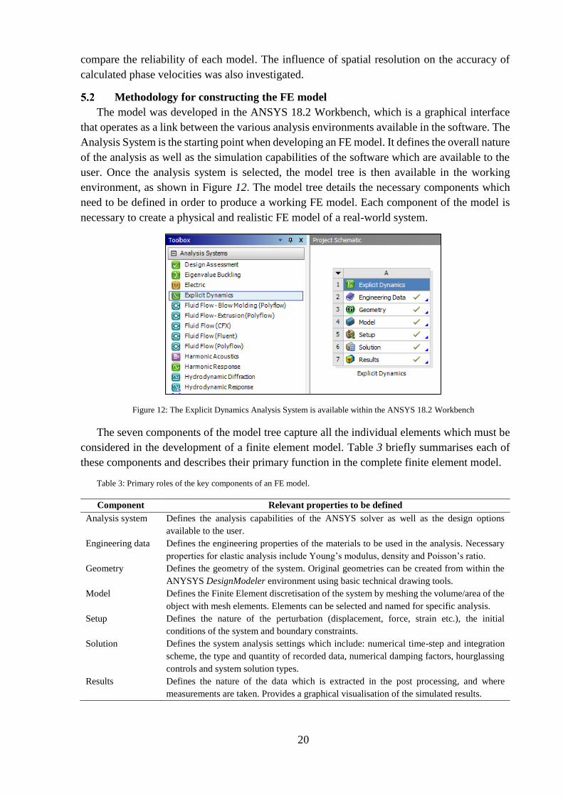
20
compare the reliability of each model. The influence of spatial resolution on the accuracy of
calculated phase velocities was also investigated.
Methodology for constructing the FE model
The model was developed in the ANSYS 18.2 Workbench, which is a graphical interface
that operates as a link between the various analysis environments available in the software. The
Analysis System is the starting point when developing an FE model. It defines the overall nature
of the analysis as well as the simulation capabilities of the software which are available to the
user. Once the analysis system is selected, the model tree is then available in the working
environment, as shown in Figure 12. The model tree details the necessary components which
need to be defined in order to produce a working FE model. Each component of the model is
necessary to create a physical and realistic FE model of a real-world system.
Figure 12: The Explicit Dynamics Analysis System is available within the ANSYS 18.2 Workbench
The seven components of the model tree capture all the individual elements which must be
considered in the development of a finite element model. Table 3 briefly summarises each of
these components and describes their primary function in the complete finite element model.
Table 3: Primary roles of the key components of an FE model.
Component Relevant properties to be defined
Analysis system Defines the analysis capabilities of the ANSYS solver as well as the design options
available to the user.
Engineering data Defines the engineering properties of the materials to be used in the analysis. Necessary
properties for elastic analysis include Young’s modulus, density and Poisson’s ratio.
Geometry Defines the geometry of the system. Original geometries can be created from within the
ANYSYS DesignModeler environment using basic technical drawing tools.
Model Defines the Finite Element discretisation of the system by meshing the volume/area of the
object with mesh elements. Elements can be selected and named for specific analysis.
Setup Defines the nature of the perturbation (displacement, force, strain etc.), the initial
conditions of the system and boundary constraints.
Solution Defines the system analysis settings which include: numerical time-step and integration
scheme, the type and quantity of recorded data, numerical damping factors, hourglassing
controls and system solution types.
Results Defines the nature of the data which is extracted in the post processing, and where
measurements are taken. Provides a graphical visualisation of the simulated results.

21
The flow chart below provides a graphical description of the main steps involved in developing
a finite element model, based on the primary components of the model tree. The order of the
steps reflects the steps taken to produce the 2D model.
Analysis system and system properties
As suggested in the Literature Review, the ANSYS Explicit Dynamics analysis system was
selected for this investigation. The system properties were then defined which govern the
overall physical nature of the system as well as the complexity of the analysis. The key system
property selections for the 2D model are shown in Figure 13.
The geometry analysis type was selected to be ‘2D’. This automatically constrains the
system to have principal directions and material properties defined in a two-dimensional plane
(default is the x-y plane). Additionally, this selection defines the 2D behaviour of the system in
the z-direction as either plane stress or plane strain depending on the user’s selection.
Explicit Dynamics analysis using the ANSYS Autodyn solver was defined in the analysis
properties. Autodyn is the ‘in-house’ explicit integration solver built into the ANSYS Explicit
Dynamics analysis environment. By default, Autodyn uses a Lagrangian integration scheme to
efficiently simulate solid elastic systems which undergo extremely high speed deformation such
as a shock [39]. Two Euler solver schemes are also available within Autodyn however these
are primarily associated with fluid flow and when simulating extreme plastic deformation [39].
a) b)
Figure 13: The Analysis System settings were configured for (a) two-dimensional geometry analysis and (b) an explicit
time integration scheme using the Autodyn solver.
Define the
Analysis
System
Define the
engineering
material data
Define the
geometry of
the model
Select and apply
the appropriate
mesh
Create named
selections
Export
results
Run the
solver
Add solution
probes to named
selections
Define the
perturbation and
apply constraints
Specify
analysis
settings

22
Engineering material properties
Selection of material properties for the FE model was driven by the requirement to validate
the accuracy of the captured data through comparison with analytical solutions in LAMSS
Waveform Revealer. In addition, it was also necessary to select a material which had been
explored within the literature to provide a baseline comparison for the physical nature of the A0
Lamb wave. Considering these criteria, the 2D FE model was developed using the material
properties of aluminium 2024-T6 (Al-2024). Al 2024-T6 is a versatile aluminium alloy used
primarily in the aerospace industry due to its high strength to weight ratio and fatigue resistance
[4]. The material properties of Al 2024-T6 were available in LAMSS Waveform Revealer,
meaning the analytical solutions of the A0 Lamb mode could be acquired. Additionally, the
propagation of Lamb waves in aluminium alloys have been thoroughly studied within the
literature by such authors including, but not limited to, Alkassar, Wilcox and Gresil [10, 12, 14,
19, 27].
The engineering material properties of the model were defined in the Engineering Data
toolbox. Finite element analysis of the elastic deformation of a material requires only three
engineering properties: Young’s modulus, density and Poisson’s ratio. This is because the
analysis is limited to the region of the material’s stress-strain curve in which the relationship
between stress and strain is approximately linear. The proportionality between stress and strain
is governed by the Young’s modulus, which represents the stiffness of the material.
The engineering material properties of aluminium 2024-T6 were sourced from the U.S.
Department of Defence MIL Handbook [40]. The material properties are summarised in Table
4 below.
Table 4: Engineering material properties of aluminium 2024-T6 [40].
Property Value
Density (𝝆) 2780 𝑘𝑔/𝑚3
Young’s modulus (𝑬) 72.4 𝐺𝑃𝑎
Poisson’s ratio (𝝂) 0.33
The properties of Al 2024-T6 were entered into the material database in ANSYS as shown in
Figure 14. The Bulk and Shear moduli are calculated automatically based on the primary
Young’s modulus and Poisson’s ratio. Once the material is stored in the database, the
engineering properties can then be assigned to the model geometry.
Figure 14: The engineering material properties of aluminium 2024 were entered into the material database in ANSYS and
assigned to the 2D model.
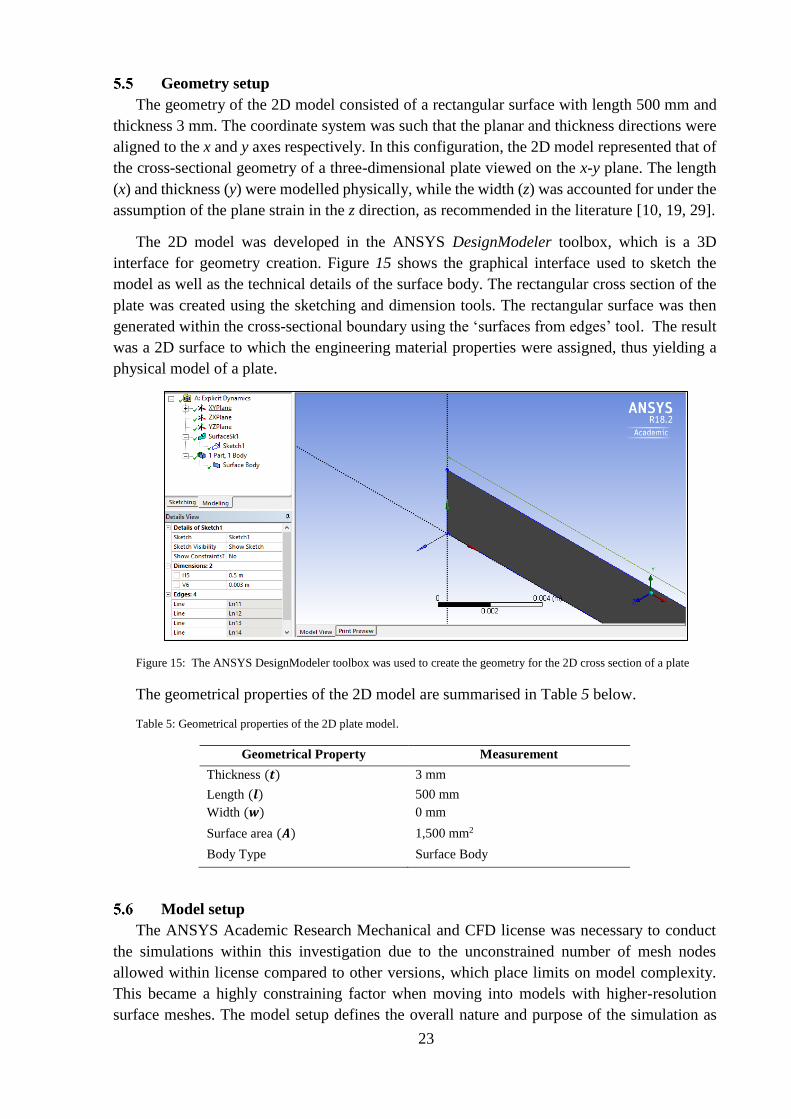
23
Geometry setup
The geometry of the 2D model consisted of a rectangular surface with length 500 mm and
thickness 3 mm. The coordinate system was such that the planar and thickness directions were
aligned to the x and y axes respectively. In this configuration, the 2D model represented that of
the cross-sectional geometry of a three-dimensional plate viewed on the x-y plane. The length
(x) and thickness (y) were modelled physically, while the width (z) was accounted for under the
assumption of the plane strain in the z direction, as recommended in the literature [10, 19, 29].
The 2D model was developed in the ANSYS DesignModeler toolbox, which is a 3D
interface for geometry creation. Figure 15 shows the graphical interface used to sketch the
model as well as the technical details of the surface body. The rectangular cross section of the
plate was created using the sketching and dimension tools. The rectangular surface was then
generated within the cross-sectional boundary using the ‘surfaces from edges’ tool. The result
was a 2D surface to which the engineering material properties were assigned, thus yielding a
physical model of a plate.
Figure 15: The ANSYS DesignModeler toolbox was used to create the geometry for the 2D cross section of a plate
The geometrical properties of the 2D model are summarised in Table 5 below.
Table 5: Geometrical properties of the 2D plate model.
Geometrical Property Measurement
Thickness (𝒕) 3 mm
Length (𝒍) 500 mm
Width (𝒘) 0 mm
Surface area (𝑨) 1,500 mm2
Body Type Surface Body
Model setup
The ANSYS Academic Research Mechanical and CFD license was necessary to conduct
the simulations within this investigation due to the unconstrained number of mesh nodes
allowed within license compared to other versions, which place limits on model complexity.
This became a highly constraining factor when moving into models with higher-resolution
surface meshes. The model setup defines the overall nature and purpose of the simulation as

24
well as the underlying physics involved in the given scenario. These model parameters are
defined in ANSYS Mechanical, which is the main interface for carrying out explicit
simulations. Figure 16 shows the Geometry and Coordinate Systems selections within the
model tree of the 2D Al 2024-T6 plate. In the Geometry options, the properties of Al 2024 were
assigned to the model by selecting the body and assigning ‘Aluminium’ from the material
library. The 2D behaviour of the model was set to plane strain which was consistent with
recommendations in the literature. The global coordinate system was selected as the default
Cartesian coordinate settings, with the x axis aligned with the principal lengthwise direction of
the plate and the y axis aligned in the thickness direction [10, 19, 29].
a)
b)
Figure 16: The ANSYS Mechanical model tree contains the model parameters which define the physics of the system.
The material selection was defined in (a) Geometry, and Cartesian coordinates were selected in (b) Coordinate System.
The surface of the 2D model was meshed using quadrilateral 4-node elements as observable
in Figure 17 (b). Each node was restricted to 2 degrees of freedom, being translation in the x
and y directions. The nodes were constrained in the z direction due to the assumption of plane
strain conditions. The mesh elements were defined as a function of the characteristic element
length as can be seen in Figure 17 (a). In the example images below, the characteristic element
length is 0.75 mm, hence over the thickness of 3 mm there are a total of 4 elements. In addition
to the pictured 0.75 mm mesh model, other models were developed having characteristic
element lengths of 1.5 mm, 1.0 mm, 0.5 mm, 0.25 mm and 0.15 mm. Simulations using
identical perturbations and analysis settings were carried out for each of the models to determine
the impact of mesh resolution on the accuracy of the simulated A0 Lamb mode. In addition, the
influence of mesh resolution on the computational efficiency of the simulation was investigated
such that the compromise between accuracy and computation speed could be better understood.

25
a)
b)
Figure 17: The 2D model of the aluminum 2024 plate was meshed using quadrilateral 4-node solid elements. The mesh
was defined by the characteristic element length, which is 0.75 mm in (a). The meshed plate is shown in (b).
To conduct a quantitative analysis of the Lamb waves generated in each simulation,
numerous nodal displacements were exported from the model. To export nodal data from
ANSYS this requires Named Selections to be defined at the particular nodes of interest to which
solution probes are then mapped. Additionally, named selections are also useful in defining the
nodes to which applied loads, or other constraints such as a fixed boundary, are applied.
In the 2D Al 2024-T6 model, the separation distance (dx) between points at which
displacement data was captured was primarily driven by the characteristic lengths of the tested
meshes. The mesh lengths were 1.5 mm, 1.0 mm, 0.75 mm 0.5 mm, 0.25 mm, and 0.15 mm,
meaning there were a number of possible separation distances which would provide whole-
number division with all mesh sizes. Initially, the spacing between points of data capture was
100 mm, making a total of 5 captured data points along the length of the plate. However, due
to the low number of data points, this meant that the variations seen in group velocity (due to
limitations in the methodology) made it difficult to establish any meaningful conclusions from
the quantitative analysis. See section 6.4.2 for a detailed discussion of the issues related to
calculation of group velocity. It was concluded that a higher spatial resolution would improve
the rigorousness of the quantitative analysis. However, due to manually selecting mesh nodes
based on x,y,z location, the creation of these named selections was found to be exceedingly time
consuming. Additionally, this process had to be repeated each time a new mesh was generated.
The spatial resolution along the length of the Al 2024-T6 plate was established at 16 equally
spaced nodes with a separation distance of 30 mm. This provided a reasonable compromise
between data resolution and time constraints for the numerous simulations. The named
selections were created on the top surface of the 2D plate as can be seen in Figure 18.

26
Figure 18: Named selections were created at 30 mm intervals along the plate. This provided 16 equally spaced nodes at
which the nodal displacement data was captured.
Selection of the excitation frequency
The centre frequency of the excitation signal was selected based on the dispersive properties
of aluminium 2024-T6, which are characterised by the phase and group velocity curves
presented in Figure 3. It was necessary to select a centre frequency such that only the
fundamental A0 Lamb mode was activated (along with the S0 mode). This is because the
presence of higher order Lamb modes in the high frequency regime can cause interference in
the measured displacement behaviour of the mesh nodes. As stated in the literature, the typical
frequency band is 2 – 200 kHz, hence the centre frequency for the 2D model testing was chosen
to be within this range [5].
Figure 20 (a) shows the phase velocity curves for Al 2024-T6. Below approximately
1714 kHz-mm only the fundamental Lamb modes exist, which is the cut-off frequency defining
the upper bound of the low-frequency regime. Taking the centre of the recommended frequency
range, at f0 equal to 100 kHz, only the fundamental modes exist. Additionally, the S0 mode
clearly travels at a much higher velocity when excited by a frequency of 100 kHz. This is
advantageous when investigating a single mode as it allows the S0 and A0 modes to be clearly
distinguished from one another. When the displacement response of a mesh node shows two
disturbances, the S0 mode would induce the first disturbance, and the A0 mode would induce
the later response. As such, a centre frequency of 100 kHz satisfied the requirements for the
phase velocity dispersive properties of Al 2024-T6. The phase velocity of the A0 Lamb mode
at an excitation frequency-thickness of 300 kHz-mm can be resolved from Figure 20 (b) at
1550 m/s.

27
a) b)
Figure 19: The phase velocity dispersion curves for Al 2024-T6 show that at an excitaton frequency of 100 kHz, only
the fundamental modes exist (a). The analytical solutions to the dispersion curves show the A0 phase velocity is 1550 m/s (b).
The excitation frequency must also satisfy the aforementioned criteria for the group velocity
dispersive characteristics of Al 2024-T6. Figure 20 (a) shows the group velocity dispersion plot
for Al 2024 from which it can be identified that the cut-off frequency, under which purely
fundamental Lamb mode propagation occurs, is approximately 1660 kHz-mm. Thus, at an
excitation frequency of 100 kHz (f-t of 300 kHz-mm) only the A0 and S0 Lamb modes will
occur. Observing Figure 20 (b), the group velocity of the fundamental antisymmetric Lamb
mode is approximately 2621 m/s at the centre frequency of 100 kHz.
a) b)
Figure 20: The group velocity dispersion plots for aluminium 2024-T6 show that at an excitation frequency of 100 kHz,
only the fundamental Lamb modes will exist (a). At this excitation frequency the group velocity is 2621 m/s (b).
Staudenmann identified that the maximum wavelength of the excitation signal, relative to
the thickness of the structure, is a key element within the criteria for Lamb wave propagation
[5]. He stated that the characteristic wavelength 𝜆0 must be sufficiently large compared to the
thickness of the structure [5]. At an excitation frequency of 100 kHz, the phase velocity of a
propagating Lamb wave in Al 2024-T6 is 1550 m/s (from Figure 3 (a)). The wavelength is
therefore calculated by;
𝜆0 =𝑐
𝑓=
1550 𝑚/𝑠
100,000 𝐻𝑧= 15.5 × 10⁻³𝑚 = 15.5 𝑚𝑚

28
As the thickness of the 2D plate is 3 mm, the ratio of wavelength to thickness is therefore
calculated by;
𝜆0
𝑡= 5.1
Thus, the ratio of wavelength to thickness is sufficiently high to validate the selection of the
central excitation frequency at 100 kHz.
Modelling the excitation frequency
The excitation signal was a nodal displacement in the thickness direction, aligned with the
y axis in global coordinates. The theoretical transducer size was arbitrarily selected at 3 mm in
diameter and was chosen to be placed on the top surface of the left-hand side of the 2D plate as
shown in Figure 21. To implement the perturbation in ANSYS, the nodal displacement loading
type was selected and applied to all surface nodes occurring within the first 3 mm from the left-
hand side of the plate. As the simulations were carried out for several mesh sizes, the number
of elements to which the nodal displacements were applied was varied accordingly. Figure 21
shows the mesh nodes (indicated with yellow labels) to which the nodal displacements were
applied for the 0.75 mm mesh size.
Figure 21: Out-of-plane (y direction) nodal displacements were applied to the mesh nodes occurring in the 3 mm from the
left-hand side of the 2D plate model.
The excitation signal was a 5-cycle sinusoidal tone burst modulated by a Hanning window
function. The signal was generated by implementing the mathematical expression given by
Equation (4) (shown again below) in a numerical algorithm using Python.
𝐴(𝑡) =𝑎
2(1 − cos (
2𝜋𝑓0𝑡
𝑁)) sin(2𝜋𝑓0𝑡)
The amplitude factor (𝑎) of the modulating function was selected small enough such that it
induced purely elastic deformation of the aluminium plate and remained realistic compared
with real-world PWAS transducers. The selected factor was 𝑎 = 1 µ𝑚, which resulted in a
propagating A0 Lamb wave with an amplitude magnitude consistent with results published by
Alkassar [10]. The centre frequency of the function was selected at 𝑓0 = 100 𝑘𝐻𝑧. The number
of cycles was selected in order to balance the pulse duration T and the width of the excitation
signal frequency spectrum. As discussed by Staudenmann, a higher number of cycles within a
pulse will result in reduced pulse-widening and better wave separation, however as 𝑇 =𝑁
𝑓0,

29
increasing the number of cycles increases the duration of the excitation [5]. This can lead to
difficulties in deciphering the incident and reflected waves if the period is too long. Hence, the
practices used in the literature were used as a guide to select N. Alkassar et al. used 𝑁 = 5
and 𝑓0 = 100 𝑘𝐻𝑧 in their simulations of the S0 and A0 modes in aluminium with excellent
agreement between analytical and simulated results [10]. Hence, the number of cycles was
selected to be 5 (𝑁 = 5) for the excitation of the A0 Lamb wave mode in the 2D plate.
The Python algorithm was developed to return a tabular response of the time and amplitude
generated by the function over the period of the excitation divided into 2000 steps. The period
of the excitation is 𝑇 =𝑁
𝑓0=
5
100,000 𝐻𝑧= 50𝜇𝑠. Hence the time-step over which the signal was
plotted is 𝑑𝑡 = 0.025𝜇𝑠. Each time step was used in Equation (4) to produce the instantaneous
amplitude of the excitation signal. The signal was then plotted in Figure 22 below.
Figure 22: The excitation signal was a 5-cycle sinusoidal tone burst modulated by a Hanning window function.
The excitation signal was modelled in ANSYS using the Tabular Data input option in the
Nodal Displacement settings. The displacement signal excitation in the ANSYS environment
is shown below in Figure 23. The tabular data was copied from the Python output and inserted
into ANSYS with the incremental variable being time. The analysis was set to last for 500 𝜇𝑠
to provide sufficient time for the incident Lamb wave to travel across the length of the plate,
reflect off the opposite boundary and return to the origin of excitation.
Figure 23: The excitation displacement amplitude was entered into ANSYS as a function of time.
Boundary constraints
A fixed support constraint was applied to the right-hand edge of the 2D plate model as
shown in Figure 24. The configuration of the model was that of a cantilever beam. This was
necessary to ensure that translation in the y direction, as a result of the excitation nodal

30
displacement, would be prevented by the reactionary force at the far end of the plate.
Consequently, when the excitation displacement is enacted on the left-hand side of the plate,
this configuration results in elastic bending.
Figure 24: A fixed support was applied to the far edge of the model to constrain the model in space.
Analysis settings
The ANSYS analysis settings control important parameters used in the solver’s explicit
integration scheme. The hourglass control was set to the Autodyn standard hourglassing
method, which is recommended for most simulation analyses. The simulation End Time was
set to 500 𝜇𝑠 to provide enough time for the propagation of the Lamb wave across the full
length of the plate and the reflection back to the excitation point. The Initial, Minimum and
Maximum Time Step settings were all set to be Program Controlled. Initially the time-step was
fixed to the critical time-step outlined in Equation (7), however the solver encountered an
“Unexpected Error” and failed to complete the analysis. Hence it was concluded that use of the
ANSYS default time-step settings would be required achieve a successful outcome.
Output controls were defined such that position data of the selected nodes would be saved
at 5000 equally spaced points within the 500 𝜇𝑠 simulation time. This meant data would be
captured at 0.1 𝜇𝑠 increments, which was found to be a reasonable compromise between data
resolution and computational efficiency of the simulation. The number of points was initially
chosen to be 500, with the resultant wave pulse shown in Figure 25 (a). Inspection of the results
clearly showed that this spatial resolution was too low to accurately capture the shape of the
Lamb wave as it passed the mesh node of interest. It can be seen from (a) that the peaks of the
wave pulse are non-physically rendered, which makes determination of certain properties such
as time of arrival more difficult. The same simulation with 5000 captured nodes is shown in
Figure 25 (b), which shows the shape of the wave pulse was accurately captured because of the
higher spatial resolution.
While 5000 points may have exceeded the minimum necessary to achieve sufficient
accuracy, the size of the simulation output was not overly constraining for the analysis. As such,
it was it was considered reasonable to be overly conservative and extract more data than
necessary, to ensure that the Lamb wave pulses were accurately captured. Additionally, the
frequency of the excitation was to be varied during the analysis, thus altering wave speed and
providing justification for using a more conservative dataset.

31
a) b)
Figure 25: The waveform was not accurately captured using 500 nodes per wavelength (a). It was found that 5000 nodes
per wavelength provided sufficient resolution to accurately capture the wave pulse as it travelled across the plate (b).
Data capture and exporting the results
The displacement-time data was captured at each of the equally spaced surface nodes, at
30 mm intervals along the plate, by assigning a Directional Deformation probe to each of the
named selections. The direction of measured deformation was set to be the y axis as the
asymmetric Lamb mode causes predominantly out-of-plane nodal displacement. The solution
results were then evaluated at each of the nodes and the results were exported to Microsoft
Excel. Since the results consistent of purely time and displacement points, the data export
involved simply copying and pasting from ANSYS into Excel.
Figure 26 provides the ANSYS results window, showing a graphical depiction of the
simulated antisymmetric Lamb mode at four points over the 500 𝜇𝑠 simulation. The data was
captured at 180 mm from the excitation. The displacement results were scaled by 30000 to see
the propagating Lamb wave, as the actual nodal displacements were in the order of 1 𝜇𝑚.
Figure 26 (a) shows the nodal displacement as the incident A0 Lamb mode first propagates
from the excitation source. Figure 26 (b) shows the nodal displacement at approximately
140 𝜇𝑠 as it nears the far end of the plate. Figure 26 (c) and (d) show the Lamb wave reflected
off the far boundary of the plate and the captured signal in the displacement results. The second
reflection is also captured as indicated by the third wave packet in the raw displacement data.
Overall, the captured data appeared realistic and physical in a qualitative sense. In all tested
mesh sizes, the solver converged to a valid solution and the simulated Lamb wave propagated
along the plate with realistic, physical behaviour. The wave travelled along the plate and
reflected off the boundary in all cases with little variation between any of the tested mesh sizes.
This indicated the differences between mesh resolution were not large enough to cause
noticeable, or largely non-physical, behaviour of the simulated Lamb wave.
The raw displacement data was exported by copying the data into an Excel spreadsheet. A
specific template was used for the data, which was arranged row-wise by time-incremental
displacement and sheet-wise by the location along the plate. The standardised format was
created in order to automate the analysis tools developed in Python for future models.

32
a)
b)
c)
d)
Figure 26: The ANSYS results window provided a graphical output of the nodal displacement data, which was used to
qualitatively analyse the propagation of the wave and make sense of the raw data.
33
6 Analysis of the two-dimensional ANSYS simulation
Overview
The analysis of the data captured in the 2D simulation involved several key elements.
Firstly, the excitation signal applied in the FE simulation was verified against the analytical
model to ensure that the perturbation was accurately modelled. The raw displacement data
captured in the simulations was then processed to produce useable data from which group
velocity and phase velocity could be determined.
Two methodologies for calculating the wave pulse group velocity were explored. The
‘reference-amplitude’ and ‘energy distribution’ approaches for time of arrival were compared
and the advantages and disadvantages of each were explored. A sensitivity analysis was carried
out to explore the reliability of each model. Using the selected approach, the group velocity of
the incident Lamb wave simulated in each of the FE models was calculated. The influence of
mesh element length on the accuracy of the simulation results was explored by comparing the
results of each model with the theoretical wave speed.
The phase velocity of the propagating Lamb wave was calculated using the two-dimensional
Fast Fourier Transform. The influence of spatial resolution on the accuracy of the obtained
results was investigated.
Where possible in the subsequent analysis, plots are presented with data pertaining to the
various FE models of different mesh resolutions. However for simplicity, many of the plots
provide the data of only one model as an example of the methodology or to demonstrate a
notable feature. The same analysis was carried out on all results to determine the influence of
mesh element resolution on the accuracy of the finite element simulations.
Verification of the excitation signal
The raw data exported from the ANSYS FE model was a tabular report of nodal
displacement as a function of time, 𝑢(𝑡). Each report contained 5000 measurements at equal
time increments recorded over the course of the simulation. The integration time step-size was
controlled by the ANSYS solver and is defined by the characteristic length of the mesh
elements. Consequently, the instantaneous time at which each measurement was taken was
variable across the six different 2D models.
Python was selected as the most capable and versatile numerical tool to process the raw
ANSYS data in semi-automated algorithm. The aim of such analysis was to yield useable results
from which the dispersive properties of the propagating Lamb wave could be understood. The
time-displacement data of nodes at which the excitation displacement was applied (𝑥 = 0 𝑚𝑚)
is shown below in Figure 27. Note, the reference point for 𝑥 = 0 𝑚𝑚 was the last excitation
node in each model, located 3 mm from the left-hand side of the beam. It can be seen that the
nodal sinusoidal tone burst shows good agreement to the mathematical expression shown in
Figure 22. It should be noted that because the excitation signal has zero displacement after
the 50 𝜇𝑠 oscillation period, the excitation nodes then become fixed in space and do not see any
further displacement when the reflected Lamb wave returns to the excitation position. This is
an inherently non-physical behaviour as the reflected signal should interact with the particles at
this location. In any case, the focus of the investigation was primarily on the incident and first
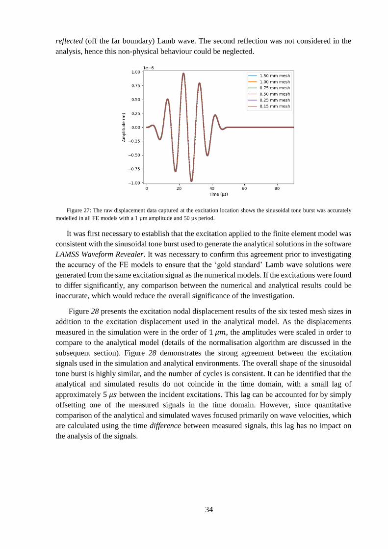
34
reflected (off the far boundary) Lamb wave. The second reflection was not considered in the
analysis, hence this non-physical behaviour could be neglected.
Figure 27: The raw displacement data captured at the excitation location shows the sinusoidal tone burst was accurately
modelled in all FE models with a 1 µm amplitude and 50 µs period.
It was first necessary to establish that the excitation applied to the finite element model was
consistent with the sinusoidal tone burst used to generate the analytical solutions in the software
LAMSS Waveform Revealer. It was necessary to confirm this agreement prior to investigating
the accuracy of the FE models to ensure that the ‘gold standard’ Lamb wave solutions were
generated from the same excitation signal as the numerical models. If the excitations were found
to differ significantly, any comparison between the numerical and analytical results could be
inaccurate, which would reduce the overall significance of the investigation.
Figure 28 presents the excitation nodal displacement results of the six tested mesh sizes in
addition to the excitation displacement used in the analytical model. As the displacements
measured in the simulation were in the order of 1 𝜇𝑚, the amplitudes were scaled in order to
compare to the analytical model (details of the normalisation algorithm are discussed in the
subsequent section). Figure 28 demonstrates the strong agreement between the excitation
signals used in the simulation and analytical environments. The overall shape of the sinusoidal
tone burst is highly similar, and the number of cycles is consistent. It can be identified that the
analytical and simulated results do not coincide in the time domain, with a small lag of
approximately 5 𝜇𝑠 between the incident excitations. This lag can be accounted for by simply
offsetting one of the measured signals in the time domain. However, since quantitative
comparison of the analytical and simulated waves focused primarily on wave velocities, which
are calculated using the time difference between measured signals, this lag has no impact on
the analysis of the signals.

35
Figure 28: Comparison of the excitation signals of the simulated and analytical models reveals good agreement in the
overall waveform, despite a small offset in the beginning of the wave packet.
To validate the excitation signal using a more rigorous methodology, the properties of the
wave packet were analysed in the frequency spectrum and the energy distributions were plotted.
An FFT algorithm was developed in Python to transform the nodal displacement data from the
time domain to the frequency domain. The resulting frequency spectrum is shown in Figure 29
(a) for the 0.15 mm mesh. Here it can be seen that the dominant frequency, at which the
amplitude of the curve is maximum, occurs at the centre frequency of 100 kHz. The amplitude
of the spectrum tapers off to zero due to the modulating effect of the Hanning window function.
The frequency bandwidth is relatively wide as indicated by the bell-shaped spectrum which
increases in amplitude from a lower bound of 60 kHz to an upper bound of 140 kHz. This means
that the excitation signal is a summation of all frequencies within the spectrum. However, it
was expected that the characteristics of the simulated Lamb wave would be driven primarily by
the dominant centre frequency of 100 kHz. Overall there is good agreement between the
analytical and simulation spectrums with both having peak amplitudes at approximately
100 kHz. Notably, some significant difficulties were encountered when plotting the frequency
spectrum of the 1.50 mm mesh, with the peak amplitude occurring well above the 100 kHz
centre frequency. This is shown in Figure 29 (b) below. It was concluded that the significant
offset was due to the methodology used to plot the frequency array which forms the horizontal
axis of the plot. The frequency increment Δ𝑓 is determined by the average time-step over all
measurements. If the time-step is inconsistent, due to the integration solver varying Δ𝑡 in order
to converge to a stable solution, this would result in the average time-step being an inaccurate
baseline to calculate Δ𝑓 as this increment would be variable. This issue was only seen in the
1.50 mm results and since the excitation signal response was qualitatively consistent (Figure
28) with the other models, it was considered a negligible limitation of the numerical analysis.

36
a) b)
Figure 29: The displacement results were transformed from the time domain to the frequency domain to reveal the
frequency spectrum of the excitation signals for (a) 0.15 mm mesh and (b) 1.50 mm mesh.
The energy distributions of the excitation signals were also plotted using the Hilbert
Function in an algorithm developed in Python. The excitation signals of the 0.15 mm and
1.50 mm meshes are shown below in Figure 30 (a) and (b) respectively. Here it can be seen
that the maximum energies occur at the centres of the wave packets at 25 𝜇𝑠. The amplitudes
of the energy envelopes return to zero after the pulses end at 50 𝜇𝑠. In both cases the simulated
responses are highly consistent with the analytical solution. Additionally, the strong agreement
between the energy distributions of the 1.50 mm model and the analytical model is supportive
of the previous claim that the offset FFT envelope was primarily attributed to numerical error.
a) b)
Figure 30: The energy envelopes of the (a) 0.15 mm mesh and (b) 1.50 mm mesh were plotted against the analytical
model, showing a high level of agreement in both models.
Qualitative comparison of the excitation responses in both time and frequency domains
showed there is a high level of agreement between the analytical and numerical models. The
results of this investigation provided justification for the baseline comparison between the
analytical and simulation results as evidence of simulation accuracy. Since the nodal
perturbation was consistent with the analytical model, comparison of Lamb wave properties
such as group velocity and phase velocity were used to characterise the accuracy of the
simulation results.

37
Signal processing of the raw data
The raw ANSYS output results provide the displacement data for each of the measured
surface nodes over the 500 𝜇𝑠 simulation time. Figure 31 is an example of the raw data captured
in the simulation of the 0.15 mm characteristic mesh length model. Figure 31 plots the nodal
displacement results measured at 𝑥 = 300 𝑚𝑚 from the excitation source, with time (𝜇𝑠) and
displacement amplitude (𝑚) plotted along the x and y axes respectively. It can be identified
from the captured data that the surface node captured three distinct wave packets over the
simulation period. Since the nodal displacement was measured along the thickness direction,
the Lamb wave packets are the antisymmetric mode, which causes primarily out-of-plane nodal
displacement. The time of arrival of the incident wave packet occurs at approximately 100 𝜇𝑠,
followed by the arrival of the reflection off the far edge of the plate at approximately 240 𝜇𝑠,
and finally the second reflection off the left edge of the plate at 440 𝜇𝑠.
The incident and reflected wave pulses clearly demonstrate that the dispersive nature of
Lamb waves was captured in the simulation. It can be observed that the beginning of the wave
pulse oscillates at a higher frequency than the tail of the wave pulse, which oscillates at a lower
frequency. This is because the high frequency components of the excitation signal (up to
140 kHz) arrive earlier, hence resulting in the high frequency oscillation at the beginning of the
wave pulse. Meanwhile, the lower frequency components of the excitation function (down to
60 kHz) arrive later, at the tail of the wave pulse. This behaviour is consistent with the
dispersive nature of Lamb waves, with higher frequencies travelling at a higher velocity than
lower frequencies (see dispersion curves provided in Figure 3). The dependency between
velocity and frequency also resulted in the wave-pulse widening captured between the incident
and reflected wave pulses in Figure 31. As the wave travelled along the plate, the velocity
difference between the high frequency and low frequency components resulted in the overall
widening of the wave pulse. This behaviour is also consistent with the results established in the
literature (see Figure 2).
Analysis of this data shows that the solver captured not only the incident Lamb wave, but
also the reflections from the boundaries. This highlights the fact that the local maxima or
minima of the incident wave packet may not be the global maxima or minima, depending on
the amplitude of the reflected waves. The implications of this consideration are discussed in
further detail below.

38
Figure 31: Nodal displacement results at x = 300 mm show the incident and reflected Lamb wave. Dispersion was
accurately captured in the simulation with velocity differences between the high and low frequencies within the wave pulses.
Figure 32 presents a close-up view of the nodal displacement shown in Figure 31, showing
the amplitude of the incident wave packet at 𝑥 = 300 𝑚𝑚 for the 0.15 mm mesh model.
Exporting 5000 data points at a 0.1 𝜇𝑠 increment resulted in a high temporal resolution of the
amplitude response of the wave pulse. The individual captured data points are plotted on the
graph by scatter points, with the solid line connecting the data points being a ‘best fit’ calculated
by the Python Matplotlib tool. It was important to achieve a high level of temporal resolution
for the signal processing of the captured Lamb waves, particularly for performing the FFT and
Hilbert transformations of the data.
Figure 32: Close-up view of the incident wave packet indicates that the 0.1µs data-capture provided good temporal
resolution of the propagating Lamb wave’s displacement amplitude.
High frequency
components Low frequency
components

39
The capability of ANSYS in modelling dispersion of the A0 Lamb wave is clearly evidenced
by observing the incident wave pulse at consecutive locations across the plate. Figure 33 shows
the displacement histories of four nodes at (a) 60 mm, (b) 120 mm, (c) 180 mm and (d) 240 mm
from the excitation source. It can be observed that the A0 Lamb wave experienced pulse
widening as it travelled across the plate, thus indicating wave dispersion. This phenomenon can
be evidenced quantitatively through determination of the period of the wave pulse at each of
these locations. The period of the wave is calculated by taking the time difference between the
beginning and end of the wave pulse, 𝑡𝑝𝑢𝑙𝑠𝑒 = 𝑡𝑒𝑛𝑑 − 𝑡𝑏𝑒𝑔. Determining these two locations
was difficult due to the small amplitudes of the high frequency oscillations at the beginning and
low frequency oscillations at the tail of the wave pulse. An algorithm was developed in Python
to capture the time data during which the nodal displacement exceeded a cut-off threshold of
1% deviation relative to the maximum nodal displacement. The initial and final times were then
used to calculate the period of the wave pulse and are indicated approximately in Figure 33.
The wave pulse period can be seen to increase consistently as the Lamb wave travels further
along the plate, with measurements of (a) 58 𝜇𝑠 at 60 mm, (b) 65 𝜇𝑠 at 120 mm, (c) 76 𝜇𝑠 at
180 mm and (d) 90 𝜇𝑠 at 240 mm. The increasing trend in period is a quantitative indication
that antisymmetric Lamb waves simulated in ANSYS Explicit Dynamics exhibit pulse
widening and, consequently, wave dispersion. However, the accuracy of these properties
compared to the analytical solutions defined by the Rayleigh-Lamb equations is yet to be
established.
a)
Δ𝑡 ≈ 58 𝜇𝑠
𝑡 ≈ 20 𝜇𝑠 𝑡 ≈ 78 𝜇𝑠

40
b)
c)
d)
Figure 33: Wave dispersion is evidenced by pulse widening between nodes located (a) 60 mm, (b) 120 mm, (c) 180
mm, (d) 240 mm from the excitation source.
Mesh size was found to have significant influence on the overall shape and speed of the
simulated A0 Lamb wave as shown below in Figure 34, which plots the nodal displacement
Δ𝑡 ≈ 65 𝜇𝑠
Δ𝑡 ≈ 40 𝜇𝑠 Δ𝑡 ≈ 105 𝜇𝑠
Δ𝑡 ≈ 76 𝜇𝑠
𝑡 ≈ 60 𝜇𝑠 𝑡 ≈ 136 𝜇𝑠
Δ𝑡 ≈ 90 𝜇𝑠
𝑡 ≈ 78 𝜇𝑠 𝑡 ≈ 168 𝜇𝑠

41
results at 𝑥 = 300 𝑚𝑚. The simulation results indicate that wave pulse group velocity
increased as mesh size was refined. The numerical results converged toward the analytical
solution consistently as mesh element length was decreased. The amplitude of the captured
displacement data also showed significant variation across the tested mesh sizes. The wave
pulse amplitude increased consistently with decreasing finite element length.
Figure 34: Comparison of the nodal displacements at 300 mm shows mesh density impacts the amplitude and speed of the
simulated wave pulse. The raw data indicates convergence toward the analytical solution as mesh length decreases.
The amplitude of a Lamb wave is directly related to the amplitude magnitude of the
excitation signal, which was defined at 1 𝜇𝑚. For this reason, the amplitudes of the measured
wave pulses were normalised to eliminate the influence of the excitation frequency amplitude
on the measured displacement data. This allowed for a more generalised analysis to be carried
out that was independent of amplitude, and purely a function of the frequency of the excitation
signal. The analytical solutions of the Rayleigh-Lamb equations were solved using LAMSS
Waveform Revealer which outputs normalised displacement data irrespective of excitation
amplitude. Since mesh size was found to directly affect the magnitude of the measured nodal
displacement, it was also convenient to normalise the signals to allow for direct comparison of
all mesh sizes to the analytical solutions, as opposed to scaling the analytical solutions to suit
each model.
Normalisation of the Lamb wave amplitude was carried out in accordance with Su’s
recommended methodology, which is to normalise the signal using the maximum magnitude of
its amplitude [2]. This is to say;
𝑢�̅� =𝑢𝑖
|𝑢𝑚𝑎𝑥|
Where 𝑢�̅� is the normalised nodal displacement, 𝑢𝑖 is the captured nodal displacement, and
𝑢𝑚𝑎𝑥 is the maximum magnitude nodal displacement captured within the wave pulse. As the

42
phase velocity and group velocity of Lamb waves are not equal in the low frequency domain,
the location of the amplitude maximum moves as the wave travels along the plate. Hence,
depending on where the measurement is taken, the maximum amplitude may be positive or
negative, which is why the absolute value was used to normalise the displacement data.
An algorithm was developed in Python to normalise the nodal displacements captured in
the ANSYS simulations. Determination of 𝑢𝑚𝑎𝑥 was challenging due to the appearance of the
reflected Lamb waves in the captured displacement data. Figure 35 shows the nodal
displacement data for the 0.15 mm mesh at 30 mm from the excitation. The incident Lamb wave
has a maximum amplitude of approximately −0.70 × 10⁻⁶ 𝑚. However, in this case the local
maximum is not equal to the global maximum of approximately 0.80 × 10⁻⁶ 𝑚, which occurs
within the reflected wave pulse at approximately 410 𝜇𝑠. As a result of this phenomena, a
functionality was required within the normalisation algorithm to differentiate the local
maximum from the global maximum when these points were not equal. This was implemented
by setting a maximum time which captured the incident Lamb wave signal but neglected the
signal of the reflected wave. This time occurs at 𝑡𝑙𝑜𝑐𝑎𝑙,𝑚𝑎𝑥 in Figure 35, which captures the
incident Lamb wave local maximum 𝑢𝑙𝑜𝑐𝑎𝑙,𝑚𝑎𝑥 and neglects the reflected global maximum
𝑢𝑔𝑙𝑜𝑏𝑎𝑙,𝑚𝑎𝑥. After the maximum amplitude is determined, the captured nodal displacements are
normalised to produce a Lamb wave pulse of maximum amplitude 1. This allowed direct
comparison with the analytical solutions.
Figure 35: An algorithm was developed to normalise the nodal displacement data using the local maximum rather than the
global maximum.
Figure 36 shows the results of the normalised wave pulse for the 0.15 mm mesh at 300 mm
from the excitation source. The maximum amplitude of the normalised incident wave packet is
unity which allows for direct comparison between the numerical and analytical results.
Qualitatively, there is strong agreement between amplitude responses of the normalised wave
packet and the analytical solution with minor deviation occurring at the tail end of the wave
pulse. The accuracy of the simulation can be measured quantitatively by determination of the
time of arrival and group velocities of the propagating Lamb waves. Figure 37 and Figure 38
𝑢𝑙𝑜𝑐𝑎𝑙,𝑚𝑎𝑥
𝑡𝑙𝑜𝑐𝑎𝑙,𝑚𝑎𝑥
𝑢𝑔𝑙𝑜𝑏𝑎𝑙,𝑚𝑎𝑥

43
show the ToA of each wave at 𝑥 = 30 𝑚𝑚 and 𝑥 = 300 𝑚𝑚 respectively, based on an
amplitude threshold cut-off of 1% relative to the maximum.
a) b)
Figure 36: Wave pulses were normalised to allow for comparison between mesh sizes and with the analytical solutions.
The 0.15 mm mesh was normalised using the local maximum (a) and shows good agreement to the analytical solution (b).
The ToA can be determined by measuring the time at which the amplitude of the wave first
reaches the cut-off threshold of 1%. It can be seen from Figure 37 that at 𝑥 = 30 𝑚𝑚 the ToA
of both simulated and analytical A0 waves are equal at approximately 11.4 𝜇𝑠. Figure 38 shows
that the two waves are travelling unequal velocities which is indicated by a difference in ToA
at 𝑥 = 300 𝑚𝑚 which was not seen at 𝑥 = 30 𝑚𝑚. The ToA of the analytical Lamb wave is
approximately 107.3 𝜇𝑠 while the ToA of the simulated wave pulse is approximately 107.5 𝜇𝑠.
The ToA measurements indicate a high level of agreement between the simulated and analytical
results with a relative error of approximately 0.18%.
By taking the difference of the ToA at the two points along the plate, the approximate group
velocities of the wave pulses can be calculated. The group velocity of the analytical model was
calculated at 2815.4 𝑚/𝑠 while the simulated wave pulse was calculated at 2809.5 𝑚/𝑠.
Hence, there was strong agreement between the analytical and simulation results. However, it
was identified that the calculated group velocities were significantly greater than the theoretical
100 kHz A0 group velocity in aluminium, at 2621 𝑚/𝑠. This suggested there were limitations
in the reference-amplitude methodology used to calculate group velocity, which was
investigated in section 6.4.

44
Figure 37: ToA at 30 mm from the excitation source was determined using a cut-off threshold of 1% at 11.4µs.
Figure 38: ToA of the analytical and simulated Lamb waves, at 300 mm from the excitation source, was determined using
a cut-off threshold of 1% at 107.3µs and 107.5µs respectively.
Determination of the simulated wave pulse group velocity
6.4.1. Reference-amplitude approach for ToA
To validate the ANSYS simulation of the A0 mode, the group velocity of the incident wave
pulse was calculated and compared with the theoretical wave speed. The group velocity was
calculated using Staudenmann’s recommended methodology. This was to take ToA
measurements at various points of known separation and using the time difference to determine
the velocity of the propagating wave pulse [5]. Staudenmann recommended that the beginning
of the wave pulse provides the most reliable point of reference for ToA of the propagating wave
[5]. This methodology was incorporated into the signal analysis Python code by storing the
instantaneous time when the normalised amplitude of the wave pulse exceeded a user-defined
reference amplitude. This process is shown graphically in the example below, which shows the
signal amplitudes at 𝑥 = 150 𝑚𝑚 for each of the tested mesh sizes. It can be seen from Figure
39 that the level of agreement between the simulation and analytical models improves as the
mesh density increases. The developed Python algorithm stores the ToA when the amplitude
𝑇𝑜𝐴
𝑇𝑜𝐴0.15𝑚𝑚 𝑇𝑜𝐴𝑎
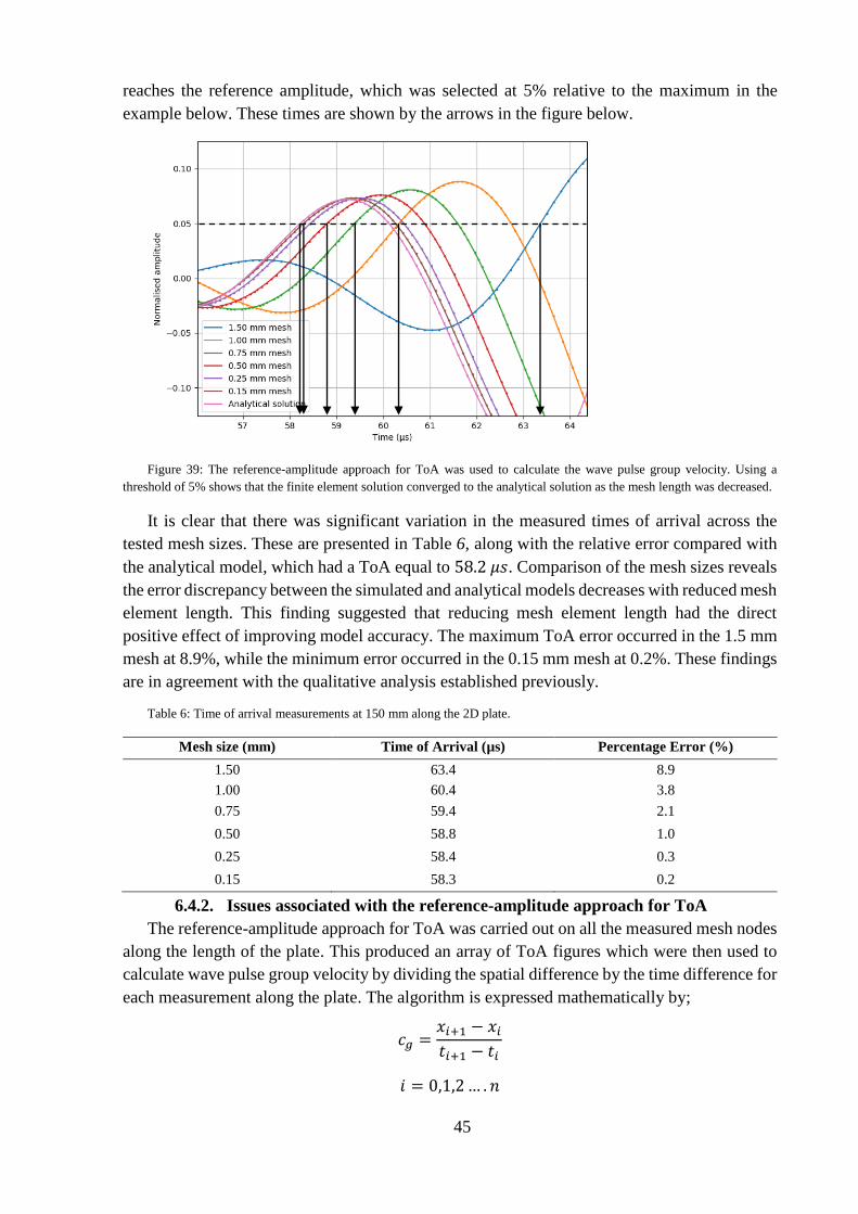
45
reaches the reference amplitude, which was selected at 5% relative to the maximum in the
example below. These times are shown by the arrows in the figure below.
Figure 39: The reference-amplitude approach for ToA was used to calculate the wave pulse group velocity. Using a
threshold of 5% shows that the finite element solution converged to the analytical solution as the mesh length was decreased.
It is clear that there was significant variation in the measured times of arrival across the
tested mesh sizes. These are presented in Table 6, along with the relative error compared with
the analytical model, which had a ToA equal to 58.2 𝜇𝑠. Comparison of the mesh sizes reveals
the error discrepancy between the simulated and analytical models decreases with reduced mesh
element length. This finding suggested that reducing mesh element length had the direct
positive effect of improving model accuracy. The maximum ToA error occurred in the 1.5 mm
mesh at 8.9%, while the minimum error occurred in the 0.15 mm mesh at 0.2%. These findings
are in agreement with the qualitative analysis established previously.
Table 6: Time of arrival measurements at 150 mm along the 2D plate.
Mesh size (mm) Time of Arrival (µs) Percentage Error (%)
1.50 63.4 8.9
1.00 60.4 3.8
0.75 59.4 2.1
0.50 58.8 1.0
0.25 58.4 0.3
0.15 58.3 0.2
6.4.2. Issues associated with the reference-amplitude approach for ToA
The reference-amplitude approach for ToA was carried out on all the measured mesh nodes
along the length of the plate. This produced an array of ToA figures which were then used to
calculate wave pulse group velocity by dividing the spatial difference by the time difference for
each measurement along the plate. The algorithm is expressed mathematically by;
𝑐𝑔 =𝑥𝑖+1 − 𝑥𝑖
𝑡𝑖+1 − 𝑡𝑖
𝑖 = 0,1,2… . 𝑛

46
The cut-off threshold, at which point the ToA was defined, was set to 5% of the maximum
amplitude. The distance, 𝑑𝑥, over which the speeds were calculated was 30 mm (equal to the
distance between each measured mesh node). The calculated group velocities were then plotted
for each of the mesh sizes in addition to the analytical model in Figure 40. There are a number
of outlying datapoints within the calculated group velocities where the velocity was found to
be significantly lower than the associated mesh average. Additionally, the first calculated group
velocity was consistently higher than the average in each of the models. For example, between
mesh nodes at 𝑥 = 180 𝑚𝑚 and 𝑥 = 210 𝑚𝑚, the group velocity calculated for the 0.15 mm
mesh was 1795 m/s. The overall average for all calculated group velocities was 2890 m/s,
representing a 37.8% deviation from the mean. Similarly, the first calculated group velocity
was 3852 m/s, thus equating to a 33.2% increase from the mean group velocity. The source of
these large discrepancies in velocity were investigated for the 0.15 mm mesh.
Figure 40: The reference-amplitude approach for ToA resulted in numerous outlying datapoints, which were attributed to
limitations in the methodology and wave dispersion.
The source of the large deviation in group velocity was explored within Figure 41 below.
Observing Figure 41 (a) and (b), which are measured at 𝑥 = 150 𝑚𝑚 and 𝑥 = 180 𝑚𝑚
respectively, it can be seen that the amplitude threshold tolerance of 5% is reached during the
second peak in the incident Lamb wave pulse. The time between (a) and (b) is approximately
10 𝜇𝑠. It can be observed from (a) – (d) that the amplitude of the second wave peak was
decreasing with time. This phenomenon is a result of attenuation and wave pulse widening
which were accurately modelled in the FE simulation. Now observing the wave pulse in (c), it
is evident that the decrease in amplitude resulted in the reference peak used in (a) and (b) being
below the 5% threshold. The ToA in this case is measured at the subsequent peak and results
in a time difference of approximately 16.7 𝜇𝑠 between (b) and (c). This increase in time
consequently resulted in the lower calculated group velocity of 1795 m/s (𝑐𝑔 =30 𝑚𝑚
16.7𝜇𝑠=
1795𝑚
𝑠). Finally, observing the measurements taken at (c) and (d) it can be seen that both are
taken on the same wave peak, resulting in a more consistent time difference of 10.8 𝜇𝑠. The
attenuative effect of decreasing amplitude results in these ‘low-velocity’ measurements in each

47
of the FE models as well as the analytical solution. This represents a significant limitation in
the reference-amplitude based approach for ToA.
a) b)
c)
d)
Figure 41: Attenuation and wave pulse widening resulted in different wave peaks being used as the reference point for
ToA. The second peak reached the 5% threshold in (a) and (b), while the third peak was measured in (c) and (d).
To investigate the accuracy of the obtained group velocities across the range of tested mesh
sizes, the percentage error associated with each of the calculated values was plotted in Figure
42. To compensate for the aforementioned deviations in velocity due to attenuation, an
algorithm was developed within the Python code to identify and remove outliers in the data
sets. The criteria for outlying data points was based on the interquartile range (IQR). If a data
point fell outside of 1.5(IQR) below the lower quartile or 1.5(IQR) above the upper quartile, it
was considered an outlier and was removed from the data set. The remaining data points were
plotted in Figure 42 (a), and the datasets were averaged to determine the overall group velocity
for each FE model.
The percentage error in group velocity was calculated relative to the theoretical group
velocity of the A0 mode in aluminium 2024-T6. Referring to the group velocity dispersion curve
in Figure 3 (b), the group velocity of the A0 mode, propagating in a 3 mm thick plate and with
a centre frequency of 100 kHz, is 2621 m/s. Hence, the percentage error of each calculated
group velocity was calculated relative to the theoretical value of 2621 m/s. The percentage error
in group velocity was then plotted as a function of position for each of the FE models in Figure
42 (b). The overall average group velocity calculated for each FE model is presented in Table
7.

48
Observation of Figure 42 (a) reveals that group velocity increased (on average) as the mesh
element length was decreased. The minimum wave speed was calculated for the 1.5 mm mesh
model at 2704 m/s (3.15% error), while the maximum wave speed was calculated for the
analytical model at 2988 m/s (14% error). Since the lowest calculated group velocity was
greater than the theoretical 100 kHz value (2621 m/s), the trend of the data seemed to suggest
that reducing the mesh element length results in greater numerical error. This was counter to
the expected trend based on the mesh element criterion (refer Equation 8). It was hypothesised
that reducing mesh element length would improve the accuracy of FE numerical simulations.
As such, the tools used to determine group velocity were investigated more closely.
a) b)
Figure 42: Wave pulse group velocity was found to increase as element length was reduced (a). Since all wave speeds
exceeded the cg of 2621 m/s, this meant numerical error increased on average as the mesh resolution improved (b).
The conclusions from the analysis initially suggested that the ANSYS simulations produced
erroneous data, as the observed trend between mesh element length and numerical error was
counter to the established literature. However, upon further inspection, this seemingly
erroneous relationship was in fact attributed to the methodology used to define the wave pulse
time of arrival. The amplitude threshold at which ToA was defined was 5% of the maximum
amplitude of the wave pulse. This meant that wave pulse ToA was defined by the first instance
of the wave packet arriving at the point of measurement. Due to the dispersive nature of Lamb
waves, higher frequency signals travel at a higher velocity through a structure, resulting in wave
pulse widening. Hence, by measuring the wave pulse ToA at 5%, the higher frequency
components of the wave pulse were measured as these frequencies travelled through the
aluminium plate at a higher speed.
The FFT of the excitation signal was provided in Figure 29, showing the centre frequency
equal to that of the ideal f0 at 100 kHz. To control spectral leakage of the excitation signal in
the frequency domain, the sinusoidal tone burst was modulated with a Hanning window
function. However, closer inspection of the frequency domain revealed spectral leakage at
higher frequencies up to 200 kHz, as shown in Figure 43. The presence of these higher
frequency components within the excitation signal could explain the convergence of the FE
models to a speed much greater than the expected 2621 m/s.

49
Figure 43: Spectral leakage causes high frequency components to exist within the wave pulse.
Table 7 presents the average group velocities for each of the mesh sizes, along with the
percentage error relative to two theoretical wave speeds; the group velocity associated with the
centre frequency (100 kHz) and the group velocity associated with the high frequency
component (190 kHz). The aluminium 2024-T6 dispersion curve was used to resolve the group
velocity at 190 kHz, at 2992 m/s. Using this wave speed, the percentage errors of the
experimentally determined group velocities were calculated.
Table 7: Average group velocity and associated error at different f0 frequencies.
Mesh size (mm) Average group velocity
(m/s)
Percentage error (%)
relative to f0 100 kHz
Percentage error (%)
relative to f0 190 kHz
1.50 2704 3.2 9.6
1.00 2876 9.7 3.9
0.75 2922 11.5 2.3
0.50 2957 12.8 1.2
0.25 2980 13.7 0.4
0.15 2982 13.8 0.3
Analytical 2988 14.0 0.1
The data presented in Table 7 supports the claim that the experimentally determined group
velocities corresponded to that of the higher-frequency components within the wave pulse. This
was a direct consequence of using the beginning of the wave pulse as a point of reference for
ToA, as the faster high-frequency components were measured prior to the centre frequency
components. The trend between mesh size and model accuracy was highly consistent with the
expected outcome when the 190 kHz group velocity was used as the ideal value.
It is clear from this analysis that defining ToA of the wave pulse based on an amplitude
threshold has a large influence on the calculated wave speed. By using a low amplitude point
of reference, the unwanted higher frequency components were measured instead of the 100 kHz
centre frequency. In order to accurately validate the group velocity of the wave pulse against
analytical results, only the 100 kHz centre frequency can be used. This is because the exact
frequency of a particular measured point in the wave pulse is difficult to accurately establish.
The percentage error of the calculated group velocity was very low compared with the 190 kHz

50
wave speed, however this is a non-rigorous approach for validating the simulation results.
Hence, this presented a major limitation in the reference-amplitude based approach for ToA
determination.
There were two primary user-defined parameters defined within the analysis; the separation
distance between nodes over which group velocity was calculated, and the amplitude threshold
at which ToA was defined. Due to the findings of this analysis, the influence of both parameters
was explored more rigorously through the sensitivity analyses below.
6.4.3. Sensitivity of reference-amplitude ToA to amplitude threshold
The amplitude threshold at which ToA is defined was varied between 10% and 90% to
investigate its impact on the calculated wave pulse group velocity. The separation distance was
fixed at 300 mm, which was found to produce the least error in group velocity for the high-
resolution meshes (discussed in section 6.4.4 below). The percentage error of the average group
velocity was calculated relative to that of the excitation frequency (100 kHz) at 2621 m/s. The
group velocity percentage error for each FE model was then plotted as a function of ToA
reference amplitude in Figure 44. Through analysis of the data presented in Figure 44, it is
clearly evident that amplitude-threshold had a significant impact on the calculated wave pulse
velocity.
Below a ToA reference amplitude of 50% all mesh models show highly chaotic variation in
group velocity accuracy. This is likely due to measuring the amplitude response triggered by
the higher-frequencies within the wave pulse. These frequencies primarily appear at the
beginning of the wave pulse due to their higher group velocity. Similarly, they induce relatively
smaller displacement amplitudes due to their lower amplitude in the frequency domain
compared to the centre frequency.
Above ToA reference-amplitudes of 50%, the 0.15 mm and 0.25 mm mesh models
converge to consistent percentage errors of 1.4% and 1.5% respectively. Similarly, at a ToA
reference amplitude of 70-90% the 0.50 mm and 0.75 mm mesh models converge to a stable
error of 2.3% and 2.4% respectively. In these regions, the reference point for ToA was near the
maximum of the wave pulse. This resulted in the group velocity being calculated primarily for
the 100 kHz centre frequency, hence the calculated group velocity was more accurate.
Additionally, at the centre of the wave pulse, the amplitudes of the high and low frequencies
are dominated by that of the centre frequency. There are insufficient data points to determine
whether the remaining FE models would converge in a similar manner.

51
Figure 44: The reference-amplitude approach was highly sensitive to the user-defined threshold at which point ToA was
defined. This was due to the amplitude response of high frequency components being measured when the threshold was low.
6.4.4. Sensitivity of reference-amplitude ToA to separation distance
The effect of separation distance was then explored to investigate its impact on the
calculation of group velocity. This involved varying the distance between mesh nodes over
which the group velocity was calculated. By increasing separation distance, the time difference
between measurements increases. However, the number of averaged group velocity data points
is reduced because the number of possible steps across the plate is reduced. The errors
associated with the average velocities were then calculated (relative to 100 kHz) and plotted in
Figure 45. It can be observed that the error largely decreases with separation distance in all of
the models, however the minimum error occurs at varying Δ𝑥. The 0.15 mm, 0.25 mm and
0.50 mm mesh models, and the analytical model, show the strongest agreement, with the
minimum error occurring at the maximum separation distance of 300 mm. This is effectively
taking samples at a spatial frequency of half the plate length and averaging the velocity. Notably
the 0.75 mm and 1.00 mm mesh models have the minimum error at a spatial separation of
270 mm, while the 1.50 mm mesh shows the highest accuracy at 90 mm.
Overall the trend of the data suggests that increasing separation distance results in an
improvement in the accuracy of the calculated group velocity. This is likely explained by the
fact that as Δ𝑥 increases, the time difference Δ𝑡 also increases. The numerical error associated
with variations in the captured amplitude peak for ToA is therefore reduced as the increase in
Δ𝑡 dampens its impact on the calculated velocity.
It is clearly evident that the calculated group velocity is highly sensitive to the separation
distance between mesh nodes. By varying the separation distance from 30 mm to 300 mm the
average change in percentage error across all models is approximately 7.2%. Thus, by selecting
the separation distance arbitrarily the calculated 𝑐𝑔 could vary, on average, by up to 7.2%. This
suggests a significant limitation in the methodology as small variations in Δ𝑥, which is often
selected arbitrarily, could vastly impact the calculation of 𝑐𝑔, leading to erroneous conclusions
when validating the simulated Lamb waves in ANSYS.

52
Figure 45: The reference-amplitude approach for ToA was highly sensitive to the separation distance over which group
velocity was calculated. Increasing separation distance resulted in a net reduction in numerical error across all models.
Through analysis of the data presented in Figure 42, Figure 44 and Figure 45 it is clearly
evident that there are significant limitations in the methodology for defining ToA based on a
reference amplitude. ToA reference amplitudes between 10-90% were shown to have a highly
significant and chaotic influence on group velocity. This was mainly attributed to higher-
frequency responses being measured when the amplitude threshold was below 50%. Separation
distance was also found to have a significant impact on the accuracy of the calculated group
velocity, suggesting that arbitrary selection of Δ𝑥 could vastly alter the measurement of group
velocity.
The highly variable and nonlinear influence of ToA reference amplitude and separation
distance led to the conclusion that arbitrary selection of these parameters would greatly reduce
the significance of the Lamb wave analysis. It was shown through the sensitivity analysis that
selection of these parameters has a significant impact on the results, and hence conclusions,
drawn from the analysis. It was therefore necessary to develop a more rigorous and reliable
methodology for measurement of the group velocity such that the accuracy of the ANSYS
simulation could be validated with confidence.
6.4.5. Energy distribution approach for wave pulse ToA
The reference amplitude approach for ToA was found to be highly sensitive to user-defined
variables such as amplitude threshold, separation distance and outlier-refinement. This meant
that there was a high level of uncertainty in any conclusions drawn from the analysis, as the
methodology used in processing the data had a significant impact on the results. Consequently,
a more robust methodology for processing the data was developed. The Hilbert function reveals
the energy distribution of the wave in the time domain. It has been shown in at least one study,
by Murat, to provide a robust tool for determining ToA [11].
A new algorithm was implemented within the signal processing Python script which took
the Hilbert function of the displacement signal at each of the measured mesh nodes. Each of the
transformed signals then represented the energy distribution of the wave as a function of time.
Figure 46 (a) and (b) provide the energy distributions of the Lamb waves, simulated using the

53
0.15 mm mesh, at 𝑥 = 30 𝑚𝑚 and 𝑥 = 150 𝑚𝑚 respectively. Observing the energy envelope
of the signal response reveals the incident Lamb wave as well as the reflections from the plate
boundaries. Similar to the methodology used in normalising the signal response, care was taken
when analysing the energy envelopes to ensure that measurements were taken at the incident
wave rather than the reflections, which in some cases had a greater amplitude
a) b)
Figure 46: Energy distribution of the measured signals at (a) 30 mm and (b) 150 mm reveal the incident and reflected
Lamb wave pulses.
Figure 47 (a) and (b) provide close-up views of the incident waves seen in Figure 46. The
energy-envelope based approach for ToA determination is illustrated in (a) and (b). The
methodology involved calculating the average time at which the energy envelope exceeded a
user-defined reference amplitude. In the below cases the threshold was 90%. By taking two
measurements on either side of the peak of the distribution, the times were averaged to
determine the approximate centre of the wave pulse. This approach provided a significantly
higher consistency of reference point for ToA as there were no issues with peak selection as
identified in Figure 41. At (a) 30 mm the two reference times are 𝑡1 = 30.8 𝜇𝑠 and 𝑡2 =
41.2 𝜇𝑠, meaning the average time is 𝑡𝑎𝑣𝑔 = 36.0 𝜇𝑠. Similarly, at (b) 150 mm the threshold
reference times are 𝑡3 = 77.1 𝜇𝑠 and 𝑡4 = 87.3 𝜇𝑠, meaning the average time is 𝑡𝑎𝑣𝑔 =
82.2 𝜇𝑠. The group velocity was then calculated by 𝑐𝑔 =𝑑𝑥
𝑑𝑡=
(150−30) 𝑚𝑚
(82.2−36.0)𝜇𝑠= 2597 𝑚/𝑠. The
percentage error compared with the theoretical velocity of 𝑐𝑔 = 2621 𝑚/𝑠 is therefore 0.90%,
which represents a high level of accuracy. This confirms the energy-distribution approach
accurately captured the velocity of the centre frequency components of the wave pulse at
100 kHz.

54
a) b)
Figure 47: The ToA was approximated by averaging the time over which the amplitude exceeded the ToA reference
amplitude. At (a) 30 mm the ToA is 36.0 µs and at (b) 150 mm the ToA is 82.2 µs.
To test the rigorousness of the energy-distribution based approach for ToA determination,
a sensitivity analysis was carried out to investigate the effect of separation distance on the error
of the calculated group velocity. The amplitude reference threshold was selected at 95% for this
study. The results are presented in Figure 48 below, which shows the relationship between
separation distance and error for the reference-amplitude methodology for ToA in (a) and the
energy-distribution methodology for ToA in (b). It is clearly evident that measuring ToA via
the Hilbert function is significantly less sensitive to separation distance than shown in (a).
Varying the separation distance between 30 mm and 90 mm causes approximately 0.5%
deviation in percentage error in all the numerical models excluding the 1.5 mm mesh. However,
increasing the separation distance from 90 mm to 300 mm resulted in almost constant relative
error with negligible deviation in all the FE models excluding the 1.5 mm mesh.
Since the analytical solution shares none of the inherent numerical error which may exist in
the FE generated data, it provides the best validation for the methodology. Observation of (b)
shows that the analytical solution is less sensitive to separation distance than all the FE models,
with a total deviation in percentage error of 0.1%. Comparing this behaviour to the reference
amplitude approach for ToA, which caused a net decrease in error of 7.8%, the energy-
distribution based approach is clearly more reliable and less sensitive to separation distance.
The significance of this attribute is highly important as the separation distance, which is
often arbitrarily selected, could affect the conclusions drawn when analysing the signal
response in applications such as SHM. Incorrect calculation of the group velocity could yield
𝑡3 𝑡4 𝑡1 𝑡2

55
inaccurate determination of material properties, false identification of damage within a structure
or inaccurate FE simulation of real-world behaviour.
a) b)
Figure 48: Sensitivity analysis of methodologies for calculating ToA based on (a) amplitude threshold and (b) Hilbert
function, reveal that the energy-distribution based approach is significantly less-sensitive to separation distance.
A second sensitivity analysis was then performed with the variable being reference
amplitude. This is the amplitude of the energy-envelope at which point time of arrival was
recorded. Figure 49 (a) and (b) present the relationship between error in calculated 𝑐𝑔 as a
function of separation distance for the reference-amplitude and energy-distribution approaches
respectively. Comparison of the two approaches reveals the energy-distribution approach was
significantly less sensitive to amplitude threshold. The maximum deviation in the error of the
analytical model was 0.5% compared with a net change of 4.0% in error in the reference-
amplitude approach for ToA. All tested FE models, excluding the 1.5 mm mesh, experienced
lower variation in percentage error with a maximum net change of 1.1% using the energy-
distribution. Using the alternative approach, the maximum net change was significantly higher
at approximately 3.7% in the 1 mm mesh. The 1.5 mm mesh shows the highest sensitivity to
amplitude threshold with a deviation of 2.3% using the energy-envelope approach. This was
still significantly lower than the original methodology, which had a net change of 4.3%.
In addition to the decreased sensitivity of the calculated 𝑐𝑔 to amplitude, the energy-
distribution approach for ToA determination also provides a significantly more consistent trend
in the data compared with the original method. While there is some deviation in the order of
accuracy when comparing the models by mesh element length, with the 0.15 mm, 0.25 mm and
0.50 mm meshes overlapping at some points, there is a significantly more consistent trend using
the energy envelope. The analytical model shows the least 𝑐𝑔 percentage error, followed by the
0.15 mm and 0.25 mm meshes, which show similar average 𝑐𝑔 percentage error. The 0.75 mm,
1.00 mm and 1.50 mm FE models then consistently increase in average error across the range
of tested reference amplitudes.
The consistent trend suggests the energy-distribution model is significantly more reliable
than the original reference amplitude approach for calculation of ToA. Having a low sensitivity
to reference amplitude is a highly important attribute of the model as arbitrary user selected
parameters should not affect the overall conclusions of the results. For example, in Figure 49

56
(a) if the user selects a reference amplitude below 50%, the order of accuracy of the FE models
is significantly different to that if the amplitude was selected above 50%. This could lead to the
same issues as discussed previously and an overall misinterpretation of the data.
Calculation of group velocity using the energy-distribution of the wave pulse was
significantly more reliable than the reference-amplitude because it ensured that the point of
reference was the 100 kHz centre frequency. This methodology suppressed the influence of the
higher-frequency components within the A0 wave pulse, even at low amplitudes. The reduced
sensitivity of the energy-envelope approach for ToA to these user defined parameters provided
evidence for its use in validation of the FE model.
a) b)
Figure 49: Sensitivity analysis of methodologies for calculating ToA based on (a) amplitude threshold and (b) Hilbert
function, reveal that the energy-distribution based approach is significantly less-sensitive to reference amplitude.
6.4.6. Validation of the 2D simulation by group velocity
The energy-distribution approach was used to calculate the ToA of the incident wave pulse
at each of the measured mesh nodes. The separation distance, over which group velocity was
calculated, was selected at 90 mm. This ensured that the sensitivity of Δ𝑥 on the calculated 𝑐𝑔
was minimised, which is shown to occur when 90 𝑚𝑚 ≤ Δ𝑥 ≤ 300 𝑚𝑚, indicated by the flat
regions Figure 48 (b). The low boundary of this range (90 mm) was chosen since having a
smaller separation distance maximises the number of data points over which the calculated 𝑐𝑔
could be averaged. The incident wave pulse ToA was also calculated using a reference
amplitude of 90%. This was because the sensitivity of average 𝑐𝑔 to reference amplitude was
shown to be within 1.1% across the entire range for the higher resolution FE models. A
reference amplitude of 90% placed the average error approximately in the centre of this small
range for the majority of the FE models. Additionally, the peak of the wave pulse was the region
of maximum energy, hence is where the amplitude response of the centre frequency is
dominant. The configuration of the model and the calculation procedure is shown in Figure 50.
The Python code used to implement this methodology is provided in Appendix A (section 15.1).

57
Figure 50: Group velocity was calculated over a separation distance of 90 mm to ensure that the influence of dx on the
measured 𝑐𝑔 was minimised.
Figure 51 (a) provides the calculated group velocities of the tested FE models as a function
of position relative to the excitation. In all of the numerical models there was a outlier occurring
at the last calculation. This was a result of the small time-difference between the incident and
reflected waves measured near the plate boundary at 𝑥 = 480 𝑚𝑚. The effect is demonstrated
in Figure 51 (b) and causes interference between the two displacement signals making it
difficult to distinguish between the incident and reflected pulses. This limitation introduces
significant error into the determination of the ToA of the incident pulse. Consequently, the data
was filtered to identify outliers based on IQR.
a) b)
Figure 51: Calculated group velocities (a) reveal erroneous data points at the far boundary of the model (a). This was
caused by interactions between the incident and reflected wave resulting in ToA error (b).
Figure 52 (a) presents the filtered group velocity data from the 2D ANSYS simulation
plotted as a function of position from the excitation. Figure 52 (b) plots the error associated
with the group velocities relative to the theoretical value of 𝑐𝑔 = 2621 𝑚/𝑠. Overall the FE
models are highly consistent with the analytical solution, with the accuracy of the simulation
increasing with improved mesh resolution. This was in agreement with the established literature
and is supportive of the hypothesis. It can be identified from the plots that the numerical solution
converged toward the analytical solution as mesh element length was reduced. This is to say
y
𝑥
Δ𝑡 Δ𝑡 Δ𝑡

58
the order of agreement with the analytical solution, from best to lowest was: the 0.15 mm,
0.25 mm, 0.50 mm, 0.75 mm, 1.00 mm and 1.50 mm FE mesh models.
a) b)
Figure 52: Using the energy-distribution of the wave pulse for ToA, the group velocities of the various FE models showed
excellent agreement with the analytical value of 2621 m/s (a). The general trend of the data was a reduction in numerical
error as the finite element length became shorter, which was consistent with expected outcomes (b).
The data sets for each model were averaged to determine the average group velocity,
percentage error and the maximum range of error (maximum error subtract minimum error)
across all captured data points. This information is summarised in Table 8 and the average
group velocities are plotted in Figure 53.
The trend of the data clearly indicates that the accuracy of the group velocity of the
simulated antisymmetric Lamb wave increases with higher mesh resolution. At the maximum
characteristic element length of 1.50 mm the percentage error is 6.66%, while the at the
minimum 𝑙𝑒 the error is 1.15%. The range of error between the minima and maxima in the data
sets also follows the same trend, with the range of error decreasing with mesh element length.
Notably, the analytical solution had a percentage error of 1.02%. This represents the inherent
numerical error within the energy-envelope methodology used to determine 𝑐𝑔. This is the
baseline error which exists within all measurements taken using this calculation procedure. As
such, the minimum error attributed to the FE simulation of the A0 Lamb wave can be adjusted
by 1.02%, which is also shown in Table 8.
Computation time was highly dependent on mesh resolution with the fastest computation at
10.4 minutes in the 1.50 mm model and the longest at 84 minutes in the 0.15 mm model. This
was due to the increased number of mesh nodes in the high resolution meshes, and
consequently, the increased complexity of the FE matrix to be solved. Due to the 2D nature of
the simulation, the computation times remained practical compared with the 3D model
(discussed in section 8.2).
Overall there is excellent agreement between the high resolution meshes with the 0.15 mm,
0.25 mm and 0.50 mm models simulating the A0 Lamb wave with less than 1% numerical error,
at 0.13%, 0.29% and 0.65% respectively. The 0.75 mm and 1.00 mm element length models
also show strong agreement with the theoretical group velocity with 1.29% and 2.37%
numerical error respectively. The maximum error occurred in the 1.50 mm model at 5.64%
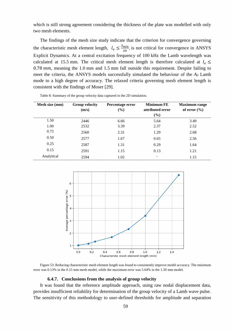
59
which is still strong agreement considering the thickness of the plate was modelled with only
two mesh elements.
The findings of the mesh size study indicate that the criterion for convergence governing
the characteristic mesh element length, 𝑙𝑒 ≤𝜆𝑚𝑖𝑛
20, is not critical for convergence in ANSYS
Explicit Dynamics. At a central excitation frequency of 100 kHz the Lamb wavelength was
calculated at 15.5 mm. The critical mesh element length is therefore calculated at 𝑙𝑒 ≤
0.78 𝑚𝑚, meaning the 1.0 mm and 1.5 mm fall outside this requirement. Despite failing to
meet the criteria, the ANSYS models successfully simulated the behaviour of the A0 Lamb
mode to a high degree of accuracy. The relaxed criteria governing mesh element length is
consistent with the findings of Moser [29].
Table 8: Summary of the group velocity data captured in the 2D simulation.
Mesh size (mm) Group velocity
(m/s)
Percentage error
(%)
Minimum FE
attributed error
(%)
Maximum range
of error (%)
1.50 2446 6.66 5.64 3.49
1.00 2532 3.39 2.37 2.52
0.75 2560 2.31 1.29 2.68
0.50 2577 1.67 0.65 2.56
0.25 2587 1.31 0.29 1.64
0.15 2591 1.15 0.13 1.21
Analytical 2594 1.02 - 1.15
Figure 53: Reducing characteristic mesh element length was found to consistently improve model accuracy. The minimum
error was 0.13% in the 0.15 mm mesh model, while the maximum error was 5.64% in the 1.50 mm model.
6.4.7. Conclusions from the analysis of group velocity
It was found that the reference amplitude approach, using raw nodal displacement data,
provides insufficient reliability for determination of the group velocity of a Lamb wave pulse.
The sensitivity of this methodology to user-defined thresholds for amplitude and separation
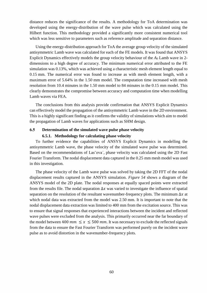
60
distance reduces the significance of the results. A methodology for ToA determination was
developed using the energy-distribution of the wave pulse which was calculated using the
Hilbert function. This methodology provided a significantly more consistent numerical tool
which was less sensitive to parameters such as reference amplitude and separation distance.
Using the energy-distribution approach for ToA the average group velocity of the simulated
antisymmetric Lamb wave was calculated for each of the FE models. It was found that ANSYS
Explicit Dynamics effectively models the group velocity behaviour of the A0 Lamb wave in 2-
dimensions to a high degree of accuracy. The minimum numerical error attributed to the FE
simulation was 0.13%, which was achieved using a characteristic mesh element length equal to
0.15 mm. The numerical error was found to increase as with mesh element length, with a
maximum error of 5.64% in the 1.50 mm model. The computation time increased with mesh
resolution from 10.4 minutes in the 1.50 mm model to 84 minutes in the 0.15 mm model. This
clearly demonstrates the compromise between accuracy and computation time when modelling
Lamb waves via FEA.
The conclusions from this analysis provide confirmation that ANSYS Explicit Dynamics
can effectively model the propagation of the antisymmetric Lamb wave in the 2D environment.
This is a highly significant finding as it confirms the validity of simulations which aim to model
the propagation of Lamb waves for applications such as SHM design.
Determination of the simulated wave pulse phase velocity
6.5.1. Methodology for calculating phase velocity
To further evidence the capabilities of ANSYS Explicit Dynamics in modelling the
antisymmetric Lamb wave, the phase velocity of the simulated wave pulse was determined.
Based on the recommendations of Lasˇova´, phase velocity was calculated using the 2D Fast
Fourier Transform. The nodal displacement data captured in the 0.25 mm mesh model was used
in this investigation.
The phase velocity of the Lamb wave pulse was solved by taking the 2D FFT of the nodal
displacement results captured in the ANSYS simulation. Figure 54 shows a diagram of the
ANSYS model of the 2D plate. The nodal responses at equally spaced points were extracted
from the results file. The nodal separation Δ𝑥 was varied to investigate the influence of spatial
separation on the resolution of the resultant wavenumber-frequency plots. The minimum Δ𝑥 at
which nodal data was extracted from the model was 2.50 mm. It is important to note that the
nodal displacement data extraction was limited to 400 mm from the excitation source. This was
to ensure that signal responses that experienced interactions between the incident and reflected
wave pulses were excluded from the analysis. This primarily occurred near the far boundary of
the model between 400 𝑚𝑚 ≤ 𝑥 ≤ 500 𝑚𝑚. It was necessary to exclude the reflected signals
from the data to ensure the Fast Fourier Transform was performed purely on the incident wave
pulse as to avoid distortion in the wavenumber-frequency plots.

61
Figure 54: The nodal responses were extracted from the model at evenly spaced points and were amalgamated in a 2D
matrix in preparation for the 2D FFT.
The results were sorted in an Excel Workbook and a Python module was developed to
implement the 2DFFT algorithm. The nodal displacement data sets were then amalgamated in
a single matrix 𝑢(𝑥, 𝑡) in row order as shown below. Note, the number of spatial points 𝑛 was
dependent on the selected Δ𝑥 which was varied from 2.5 mm to 40 mm. The maximum time 𝑡𝑘
was selected at 220 𝜇𝑠 to exclude the reflection from the incident wave pulse in all nodal
displacement results.
𝑢(𝑥, 𝑡) =
[ 𝑥1(𝑡0) 𝑥1(𝑡1) 𝑥1(𝑡2) ⋯ 𝑥1(𝑡𝑘)𝑥2(𝑡0) 𝑥2(𝑡1) 𝑥2(𝑡2) ⋯ 𝑥2(𝑡𝑘)𝑥3(𝑡0) 𝑥3(𝑡1) 𝑥3(𝑡2) ⋯ 𝑥3(𝑡𝑘)
⋮ ⋮ ⋮ ⋯ ⋮𝑥𝑛(𝑡0) 𝑥𝑛(𝑡1) 𝑥𝑛(𝑡2) ⋯ 𝑥𝑛(𝑡𝑘)]
The 2D FFT was then implemented on the matrix 𝑢(𝑥, 𝑡) to transform the displacement
results from the time-space domain to the wavenumber-frequency domain as shown below.
𝐻(𝑘, 𝑓) = ∫ ∫𝑢(𝑥, 𝑡)𝑒−𝑖(𝑘𝑥−𝜔𝑡)𝑑𝑥 𝑑𝑡
The resultant matrix was populated with complex numbers whose magnitude revealed the
Lamb wave pulse in the wavenumber-frequency domain. The magnitude of 𝑢(𝑥, 𝑡) was graphed
on a contour plot as a function of wavenumber (1/𝑚) and frequency (MHz). The complete
Python code of the 2DFFT implementation is provided in Appendix B (see section 15.1).
6.5.2. Influence of spatial resolution on the wavenumber-frequency domain
Spatial resolution is controlled by the separation distance Δ𝑥 between the nodes at which
displacement data is captured. A higher spatial resolution means the step size between mesh
nodes is smaller. The matrix 𝑢(𝑥, 𝑡) is therefore populated with more data which impacts the
resolution of the transformed response in the wavenumber-frequency domain. Costley noted
that a sufficiently high spatial resolution is necessary to avoid aliasing in the resultant
wavenumber-frequency domain [36]. The separation distance Δ𝑥 was varied from 2.5 mm to
40 mm to investigate the spatial requirements for the simulated antisymmetric Lamb wave in
ANSYS. The FE model having a characteristic mesh element length of 0.25 mm was used in
the sensitivity analysis as it provided a convenient integer division with the Δ𝑥 distances.
The scope of the testing is summarised in Table 9. Provided is the separation distance Δ𝑥,
the number of captured mesh nodes between 0 𝑚𝑚 ≤ 𝑥 ≤ 400 𝑚𝑚, the spatial resolution
normalised in nodes per 100 mm, and the spatial resolution in nodes per (nominal) wavelength
where 𝜆 = 15.5 𝑚𝑚.
Δ𝑥
y
𝑥
1 2 3 4 5 6 7 8 9 10 11… 𝑛

62
Table 9: Scope of the spatial resolution sensitivity analysis.
Separation distance
(mm)
Number of mesh nodes Mesh nodes per 100 mm Nodes per wavelength
40 11 2.75 0.39
30 14 3.59 0.52
20 21 5.25 0.78
15 27 6.92 1.03
12.5 33 8.25 1.24
10 41 10.25 1.55
7.5 53 13.59 2.07
5 81 20.25 3.1
2.5 161 40.25 6.2
The wavenumber-frequency contour plots for each tested Δ𝑥 are provided by Figure 56 and
Figure 57. These plots are useful as the phase velocity 𝑐 can be resolved directly by using the
relation 𝑐 = 𝜔/𝑘. The sensitivity analysis revealed that the resultant wavenumber-frequency
plot, and consequently the calculated phase velocity, is highly dependent on the spatial
resolution of the 2D FFT. Specifically, it was found that the number of nodes per (nominal)
wavelength had to be at least 1 to produce a wavenumber-frequency plot from which the
calculated phase velocity was physical.
The theoretical phase velocity was approximated from the aluminium 2024-T6 dispersion
curve at 1550 m/s. The methodology for calculating phase velocity using the wavenumber-
frequency plots is demonstrated below.
Figure 55 shows a closeup view of the k-f plot for Δ𝑥 = 2.5 𝑚𝑚. The colour of each contour
in the k-f plot represents its magnitude relative to the maximum amplitude. Blue contours
represent those with minimal or nil amplitude, green represents those with moderate relative
amplitude, and yellow indicates contours of maximum amplitude. The contour of maximum
amplitude in the k-f plot defines the frequency within the spectrum at which the wave energy is
maximum. This should theoretically occur at the central excitation frequency of 100 kHz.
As a consequence of using a finite number of spatial and time measurements in the 2D FFT,
aliasing occurs in the response which causes the k-f plot to have a coarse resolution. This
limitation in plot resolution introduces a range of uncertainty in both wavenumber and
frequency as indicated by the arrows in
Figure 55. It can be seen in the below example that the centre excitation frequency of
100 kHz lies within the bounds of the contour of maximum amplitude. However, due to the
limited resolution of the plot, there exists a range of valid frequencies for the contour. This
means there may be some degree of error between the apparent frequency of maximum wave
energy and actual frequency of the excitation.

63
Figure 55: Closeup view of the wavenumber-frequency plot reveals a range of uncertainty which is attributed to the spatial
resolution.
Wavenumber-frequency plots were generated for each of the tested spatial resolutions and
are provided below. Each of the various k-f plots could be easily discerned and classified in one
of two distinct groups, being physical and non-physical. When the spatial resolution was less
than 1 node per wavelength, the plots indicated non-physical behaviour of the simulated Lamb
wave. When the spatial resolution was greater than 1 node per wavelength, the data indicated
mostly physical behaviour of the Lamb wave. Hence, there was a clear discrepancy between
the data sets across this spatial criterion. For this reason, the k-f plots are separated between
Figure 56 and Figure 57. Figure 56 (a), (b) and (c) present the k-f plots for Δ𝑥 distances of
40 mm, 30 mm and 20 mm respectively. Figure 57 (a), (b), (c), (d), (e) and (f) present the k-f
plots for Δ𝑥 distances of 15 mm, 12.5 mm, 10 mm, 7.5 mm, 5 mm and 2.5 mm respectively.
The full k-f domain is shown in each plot, in addition to a close-up view of the contour of
maximum amplitude with the ranges of uncertainty in k and f indicated by arrows. The actual
excitation frequency is also plotted at 100 kHz.
a) b)

64
c)
Figure 56: A spatial resolution of less than 1 node per wavelength resulted in the indication of non-physical bahviour of
the Lamb wave. This occurred for separation distances of (a) 40 mm, (b) 30 mm, and (c) 20 mm.
a)
b) ``
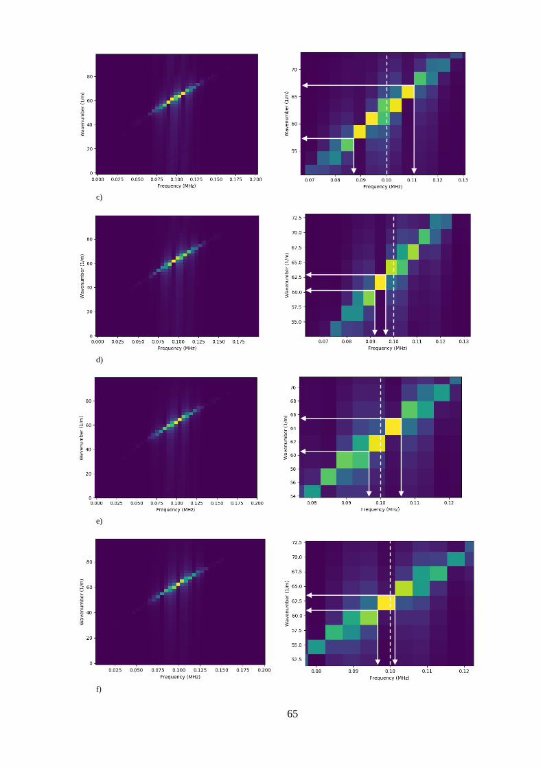
65
c)
d)
e)
f)
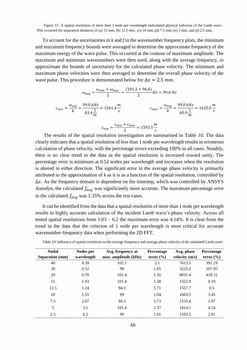
66
Figure 57: A spatial resolution of more than 1 node per wavelength indicatated physical bahviour of the Lamb wave.
This occurred for separation distances of (a) 15 mm, (b) 12.5 mm , (c) 10 mm, (d) 7.5 mm, (e) 5 mm, and (f) 2.5 mm.
To account for the uncertainties in k and f in the wavenumber frequency plots, the minimum
and maximum frequency bounds were averaged to determine the approximate frequency of the
maximum energy of the wave pulse. This occurred at the contour of maximum amplitude. The
maximum and minimum wavenumbers were then used, along with the average frequency, to
approximate the bounds of uncertainty for the calculated phase velocity. The minimum and
maximum phase velocities were then averaged to determine the overall phase velocity of the
wave pulse. This procedure is demonstrated below for Δ𝑥 = 2.5 𝑚𝑚.
𝜔𝑎𝑣𝑔 =𝜔𝑚𝑖𝑛 + 𝜔𝑚𝑎𝑥
2=
(101.3 + 96.6)
2𝐻𝑧 = 99.0 𝐻𝑧
𝑐𝑚𝑖𝑛 =𝜔𝑎𝑣𝑔
𝑘=
99.0 𝑘𝐻𝑧
63.41𝑚
= 1561.4𝑚
𝑠
𝑐𝑚𝑎𝑥 =𝜔𝑎𝑣𝑔
𝑘=
99.0 𝑘𝐻𝑧
60.91𝑚
= 1625.5𝑚
𝑠
𝑐𝑎𝑣𝑔 =𝑐𝑚𝑖𝑛 + 𝑐𝑚𝑎𝑥
2= 1593.5
𝑚
𝑠
The results of the spatial resolution investigation are summarised in Table 10. The data
clearly indicates that a spatial resolution of less than 1 node per wavelength results in erroneous
calculation of phase velocity, with the percentage errors exceeding 100% in all cases. Notably,
there is no clear trend in the data as the spatial resolution is increased toward unity. The
percentage error is minimum at 0.52 nodes per wavelength and increases when the resolution
is altered in either direction. The significant error in the average phase velocity is primarily
attributed to the approximation of k as it is as a function of the spatial resolution, controlled by
Δ𝑥. As the frequency domain is dependent on the timestep, which was controlled by ANSYS
Autodyn, the calculated 𝑓𝑎𝑣𝑔 was significantly more accurate. The maximum percentage error
in the calculated 𝑓𝑎𝑣𝑔 was 1.35% across the test cases.
It can be identified from the data that a spatial resolution of more than 1 node per wavelength
results in highly accurate calculation of the incident Lamb wave’s phase velocity. Across all
tested spatial resolutions from 1.03 – 6.2 the maximum error was 4.14%. It is clear from the
trend in the data that the criterion of 1 node per wavelength is most critical for accurate
wavenumber-frequency data when performing the 2D FFT.
Table 10: Influence of spatial resolution on the average frequency and average phase velocity of the simulated Lamb wave.
Nodal
Separation (mm)
Nodes per
wavelength
Avg. frequency at
max. amplitude (kHz)
Percentage
error (%)
Avg. phase
velocity (m/s)
Percentage
error (%)
40 0.39 102.1 2.1 7613.5 391.19
30 0.52 99 1.05 3223.2 107.95
20 0.78 101.4 1.35 8031.4 418.15
15 1.03 101.4 1.38 1552.9 0.19
12.5 1.24 94.3 5.71 1557.7 0.5
10 1.55 99 1.04 1603.5 3.45
7.5 2.07 94.3 5.73 1533.4 1.07
5 3.1 101.4 1.37 1614.1 4.14
2.5 6.2 99 1.01 1593.5 2.81

67
Figure 58 (a) presents the effect of spatial resolution on the average frequency at which the
maximum wave energy was recorded in the k-f plots. One of the fundamental requirements for
k-f plot is agreement between the central excitation frequency and the frequency at which the
wave energy is maximised. Overall, the relationship between spatial resolution and average
phase velocity is unclear within the scope of the data. While the minimum error in frequency
occurs for the highest resolution model, at 1.01% for Δ𝑥 = 2.5 𝑚𝑚, the error in 𝑓𝑎𝑣𝑔 varies
chaotically as Δ𝑥 increases. The frequency range also varies significantly with resolution. When
the separation distance was 2.5 mm, 7.5 mm, and 12.5 mm, a single contour of maximum
amplitude was plotted hence resulting in a narrow frequency band. Models having separation
distance of 5 mm and 15 mm both showed a wider frequency band with 2 contours of equally
large magnitude. Notably the 10 mm model showed 4 nodes of maximum amplitude either side
of the 100 kHz central frequency, resulting in the widest frequency range.
Figure 58 (b) presents the effect of spatial resolution on the average phase velocity. Like
the average frequency, there is no discernible relationship between phase velocity and spatial
resolution seen within the scope of the testing. The most accurate approximations of phase
velocity occurred when Δ𝑥 = 15 𝑚𝑚 at 0.19% which was contrary to the expected outcome.
The accuracy of the calculated phase velocity varies nonlinearly with spatial resolution with the
maximum error occurring when Δ𝑥 = 5 𝑚𝑚.
Overall, no significant trends were noted between spatial resolutions greater than 1 node per
wavelength and the average frequency or phase velocity of the Lamb wave pulse. It is
hypothesised that this result was likely due to the scope of the testing covering an insufficient
spatial resolution range to see significant impact on the accuracy of the numerical model. In the
research carried out by Lasˇova´, the displacements of all 4096 mesh nodes were captured and
used in the 2D FFT when it was shown that increasing the resolution increased the accuracy of
the dispersion curves [14]. This level of resolution could not be reached in this analysis due to
time and computational constraints. It is possible that a significantly higher resolution needs to
be attained before spatial resolution begins to largely affect the accuracy of the generated k-f
plots.
Within the scope of the data gathered in the investigation, the relationships between spatial
resolution and average phase velocity and frequency are unclear. The data indicates that within
the tested range of Δ𝑥, spatial resolution has little influence on the average phase velocity. At
all spatial resolutions from 1.03 to 6.2 nodes per wavelength the calculated average frequency
and phase velocity were within 5.73% and 4.14% of the theoretical values respectively. This
finding suggests that future investigations requiring only approximations of phase velocity
could validly use spatial resolutions within the tested range. The most notable criteria for spatial
resolution found within the investigation is that at least 1 node per wavelength is required to
yield physical approximations of phase velocity.

68
a) b)
Figure 58: The influence of spatial resolution on (a) average frequency and (b) phase velocity is unclear. This may be
attributed to the scope of the testing covering an insufficiently fine spatial resolution.
6.5.3. Validation of the 2D ANSYS simulation by phase velocity
Through a sensitivity analysis it was found that the average frequency and phase velocity
were calculated to a high degree of accuracy when the spatial resolution was higher than 1 node
per wavelength. As a result of this conclusion, the 0.25 mm model was analysed further to
validate the accuracy of the ANSYS simulation of the fundamental A0 Lamb mode.
Table 10 presented the phase velocities calculated from each of the k-f plots along with the
percentage errors relative to the theoretical Lamb wave velocity. In aluminium 2024-T6, this is
1550 𝑚/𝑠. The calculated phase velocity with the minimum associated error was 𝑐 =
1552.9 𝑚/𝑠 at only 0.19% compared to the theoretical value. The maximum error occurred for
𝑐 = 1614.1 𝑚/𝑠 at 4.14%. These findings suggest that ANSYS Explicit Dynamics is highly
effective in accurately modelling the phase dispersion characteristics of the A0 Lamb wave. The
findings from the spatial resolution investigation suggest that nodal displacement data captured
in ANSYS can be reliably used to approximate Lamb wave phase velocity assuming at least 1
node exists per wavelength.
The numerical error in group velocity calculated for the 0.25 mm mesh ANSYS model was
somewhere between 0.35% and 1.37%, depending on the inherent error in the methodology.
Comparison of the group velocity error range to that of phase velocity, which is between 0.19%
and 4.14%, suggests an acceptable level of consistency between the two approaches. As the
phase velocity and group velocity are two independent characteristics of the Lamb wave, this
analysis further validates the capabilities of ANSYS in modelling the fundamental
antisymmetric Lamb wave.
The methodology used to calculate group velocity was more rigorously optimised than that
used to calculate phase velocity, which may explain why the error in 𝑐𝑔 is lower than the error
in 𝑐. Despite this, the degree of accuracy seen in the phase velocity was reasonably high
considering the maximum mesh node resolution was only 6.2 nodes per wavelength. It is
hypothesised that increasing the data resolution to capture all nodal displacement results would
improve the overall resolution of the wavenumber-frequency plots. Hence, this would yield
calculated phase velocities at an even higher degree of accuracy. Verification of this hypothesis
is suggested for future research investigations.

69
7 Development of the three-dimensional ANSYS model
Overview of the study
Lamb wave-based SHM techniques typically utilise a network of transducers that emit and
detect guided waves along the surface of a structure. The sensor arrangement is often
multidirectional to ensure that the entire surface is captured by the network. Complex transducer
networks are often required to monitor composite structures due to their anisotropic nature and
hence more complicated wave propagation. This means that a finite element models of Lamb
waves must reach the complexity of three-dimensions to capture the real-world propagation
behaviour of Lamb waves. Three-dimensional FE models also allow more complex wave
scattering from boundaries such as edges and joins which exist in real-world structures.
To investigate the simulation capabilities of ANSYS in modelling the A0 Lamb mode in
three-dimensions, the analysis was performed using a 3D model of the aluminium 2024 plate.
This analysis provided validation of ANSYS Explicit Dynamics in modelling Lamb waves
using higher order mesh elements which allow propagation in the z direction. The results of this
study aim to validate the use of ANYS Explicit Dynamics to model the multidimensional
propagation of Lamb waves in SHM transducer networks.
Analysis settings, material properties and geometry
The 3D FE model was developed using predominantly the same analysis settings,
constraints and material properties as the 2D plate. This was to ensure that any significant
differences between the results of the 2D and 3D simulations could be attributed to specific
variables within the models with a high degree of confidence. Figure 59 (a) shows the model
properties for the 3D simulation with the Analysis Type set to ‘3D’. In setting this property the
z-direction plane strain criterion is turned off, thus allowing the numerical model to simulate
wave propagation in both x and z directions. This occurs by introducing a third degree of
freedom for displacement (z) to each of the FE mesh nodes. The x, y and z displacements are
solved by the FEM equations of motion, which are then more complex due to the added DOF.
The geometry of the 3D model is shown in Figure 59 (b). The model was a square plate with
equal side lengths of 400 mm in the x and z directions. The thickness of the plate was 3 mm in
the y direction. The thickness was kept equal to that of the 2D model due to its influence on
dispersive wave properties (𝑐 and 𝑐𝑔). The plate material was aluminium 2024-T6 and had the
same engineering properties as presented in Table 4.

70
a) b)
Figure 59: The FE model properties were set to 3D to capture the propagation of Lamb waves through the x-z plane (a).
The model was a square plate with dimensions 400 mm × 400 mm × 3 mm (b).
Model setup
The 3D plate geometry was imported into ANSYS Mechanical for the Model Setup. The
geometry was meshed using 8-node SOLID45 brick elements. Each of the mesh nodes had
3DOF, thus allowing translation in the x, y and z directions. The characteristic mesh element
length was selected based on two primary criteria: accuracy of the simulation results and
computation time. In the 2D investigation, all models produced relatively accurate simulation
results (highest FE error was 5.64%), however computation time ranged from 10.4 to 84
minutes depending on the mesh resolution. The 1 mm element length model was selected as
having the most favourable compromise between accuracy and efficiency, with an FE error of
2.37% and computation time of 52.8 minutes. A characteristic mesh element length of 1.0 mm
was therefore selected for the three-dimensional study. This resulted in a typical computation
time of around 8 hours for 3D simulations, which was the longest feasible time given the
number of test cases within the scope of the investigation. Figure 60 shows the 3D aluminium
plate meshed with 3 elements in the thickness direction, each having 𝑙𝑒 = 1.0 𝑚𝑚.
Figure 60 also shows the nodal displacement excitation which was applied to the centre
surface-node along the left-hand boundary of the pate. The excitation was a sinusoidal tone
burst modulated with a Hanning window function. The centre frequency was kept at 100 kHz
to provide a direct comparison between the 2D and 3D models. The far boundary of the plate
was constrained using a Fixed Support to provide the necessary reaction force against the nodal
displacement excitation.
The explicit integration solver was ANSYS Autodyn, with the settings kept the same as the
2D model to provide consistency. The time-step was set to computer controlled as were FE
variables such as hourglassing control and numerical damping. Named Selections were created
at equally spaced points along the length of the plate, with 𝑑𝑥 = 10 𝑚𝑚.

71
Figure 60: The characteristic mesh element length was 1 mm to provide an acceptable compromise between accuracy and
computational time.
Simulation results
The 100 kHz excitation frequency was applied to the surface of the 3D plate model and the
resultant Lamb wave propagation was captured over 220 𝜇𝑠. This simulation time allowed for
the incident wave to travel across the length of the plate to the far boundary. The nodal
displacement results at equidistant points along the plate were captured and the data was
exported for analysis in Python. Figure 61 shows the propagation of the fundamental
antisymmetric Lamb mode at 120 mm from the excitation source. The displacement is scaled
by a factor of 15,000 to provide a visual depiction of the wave packet. Here it can be seen that
the Lamb wave propagates in a radial direction from the source along the x-z plane. From a
qualitative standpoint, the simulated Lamb wave appears consistent with the 2D model and
behaves in a physically realistic manner. Figure 61 also shows nodal displacement in the y
direction captured in the ANSYS simulation at 𝑥 = 120 𝑚𝑚. The first excitation is the incident
Lamb wave packet which occurs at 43 𝜇𝑠. The second displacement excitation is due to
reflections from the side boundaries of the plate which meet at the centre at 160 𝜇𝑠. The
boundary reflections can be seen in Figure 62. Note that this reflected signal was not seen in
the 2D simulation, with the only reflection being that from the far boundary of the plate.

72
Figure 61: The nodal displacement in the thickness direction was measured to capture the antisymmetric Lamb wave as it
propagated along the plate.
The Lamb wave packets reflected from the side boundaries of the 3D model add complexity
to the signal processing which was not seen in the 2D model. This was the driving factor in
reducing the overall simulation time to 220 𝜇𝑠. After this point, significant noise was
introduced in the captured nodal displacement data due to subsequent interactions with the plate
boundaries. The model validation focused primarily on the dynamics of the incident Lamb
wave. This data was therefore omitted, thus reducing the overall simulation time required.
Figure 62: Reflections from the side boundaries of the plate introduced complexity into the 3D model which was not seen
the 2D model. This required more deliberate selection of the simulation time to avoid noise in the displacement data.
8 Analysis of the three-dimensional ANSYS simulation
Signal processing of the raw data
The nodal displacement data captured in the 3D simulation was exported from ANSYS for
signal processing in Python. The methodology for analysing the data was similar to that used
for the 2D model. The incident wave packet was first identified within each of the signals and
the maximum amplitude of the pulse was then used to normalise the entire data set. The
displacement histories were then plotted against the analytical solution to provide a visual
comparison of the wave pulse. Figure 63 (a) presents the raw data measured at 60 mm from the

73
excitation source. The incident and reflected waves can be clearly distinguished at this mesh
node. The incident wave pulse had a maximum amplitude 2.3 × 10⁻⁸ 𝑚 which was then used
to normalise the amplitude, as shown in Figure 63 (b). Comparing the simulated wave pulse
with the analytical solution reveals very strong agreement between the shape of the A0 mode at
this location. The number of peaks within the wave pulse and the overall effect of wave pulse
widening as a result of dispersion is accurately captured by the simulation. The most notable
discrepancy occurs at the second peak in the wave pulse, which has a shallower amplitude in
the numerical model as compared with the analytical waveform.
The wave pulse period of the analytical model at 𝑥 = 60 𝑚𝑚 is 45.8 𝜇𝑠, while the period
is 46.6 𝜇𝑠 for the numerical wave pulse. The error in wave pulse period is therefore only 0.8 𝜇𝑠.
This suggests that wave dispersion was accurately modelled in the 3D simulation.
a) b)
Figure 63: The raw data captured at 60 mm from the excitation reveals the incident and reflected wave pulses (a). The
wave pulse was normalised and compared with the analytical solution, revealing excellent agreement overall (b).
Figure 64 (a) and (b) plot the raw and normalised data captured at 200 mm from the
excitation source. Here the separation between the incident and reflected waves is much lower,
which was considered during normalisation. Comparison of the numerical and theoretical wave
pulses reveals a noticeable lag of approximately 2 𝜇𝑠 which did not exist at 60 mm (Figure 63).
The earlier ToA of the analytical wave pulse indicates that the simulated A0 Lamb wave is
travelling at a lower group velocity than the analytical solution. Despite this, the dispersive
effect of wave pulse widening is still modelled highly accurately at 𝑥 = 200 𝑚𝑚, with pulse-
periods of 59.8 𝜇𝑠 and 61.4 𝜇𝑠 for the analytical and numerical models respectively. The error
between pulse-widths is therefore 1.6 𝜇𝑠 which is only a 0.8 𝜇𝑠 increase in error between
measurements at 𝑥 = 60 𝑚𝑚 and 𝑥 = 200 𝑚𝑚 from the excitation. This finding suggests that
ANSYS accurately models the wave-pulse widening effect of dispersion with an acceptable
level of numerical error. However, it also indicates that simulating Lamb wave propagation
over longer distances could lead to an increase in overall error in the shape of the wave pulse.

74
a) b)
Figure 64: The nodal displacement data captured at 200 mm (a) reveals the simulated wave pulse travelled with a lower
velocity as indicated by the lag between wave packets (b).
Model validation and comparison of results with the 2D model
The incident Lamb wave was plotted at each point along the plate and was normalised by
the maximum amplitude to provide a comparison between the 2D, 3D and analytical models.
The Hilbert transformation of each captured signal was taken to reveal the energy envelope of
the incident Lamb wave. The energy-distribution of the wave pulse was also used to compare
the models via group velocity. Figure 65 presents a comparison of the normalised Lamb wave
measured at two locations along the plate: (a) 40 mm from the excitation and (c) 180 mm from
the excitation. The Hilbert transformations are also plotted in (b) and (d).
There is strong consistency between the 2D and 3D models at both locations along the plate.
The number of peaks within the Lamb wave amplitude, along with the overall shape and period
of the wave pulse, indicates strong agreement between the two models. The time lag between
the 2D and 3D simulations remains consistent between the two measured points along the plate
with Δ𝑡40 = 1.6 𝜇𝑠 and Δ𝑡180 = 1.7 𝜇𝑠, indicating that the velocity difference between the two
wave pulses is not significant.
Analysis of the energy envelope of the 3D simulation results, reveals significant aliasing in
the response which was not seen in the 2D model results. The overall amplitude and location
of the energy distribution is consistent between the models, however there is a large amount of
noise within the amplitude of the 3D model. It was hypothesised that the introduction of a third
degree of freedom, being translation in the z-direction, resulted in an additional source of
numerical error into the displacement results. This is discussed in further detail below.

75
a) b)
c) d)
Figure 65: Comparison of the wave pulses at (a) 40 mm and (c) 180 mm reveals an overall consistency in the shape of
the Lamb waves simulated in the 3D and 2D models. The energy distributions of the wave pulses (b) and (d) show that there
was aliasing seen in the 3D model which was attributed to numerical error.
The energy distribution approach for ToA was used to calculate the group velocity of the
incident Lamb wave simulated in the ANSYS 3D model. Graphs plotting the calculated group
velocity at each measured mesh node along the length of the plate, for both the 2D and 3D
models, are provided in Appendix C (section 15.3). The group velocities calculated at all points
along the plate were averaged to determine the overall group velocity of the simulated
antisymmetric Lamb wave. Table 11 summarises the findings of the study. The average group
velocity of the incident Lamb wave simulated in the 3D model was 2503 m/s, which
corresponds to a 4.49% error compared with the theoretical value. By subtracting the baseline
error of 1.02% measured in the analytical model, the minimum error attributed to the FE
simulation was 3.47%. Comparing this with the 2D model, which had a minimum FE error of
2.37%, the two simulations yield highly consistent results. The difference in calculated group
velocities is 29 m/s (1.1%), with the wave pulse simulated in the 3D environment having the
lower velocity.
Table 11: Comparison of average group velocities calculated in the 2D and 3D simulations.
Model type Group velocity (m/s) Percentage error (%) Minimum FE attributed error (%)
2D 2532 3.39 2.37
3D 2503 4.49 3.47
Analytical 2594 1.02 -

76
The primary explanation of the increased error seen in the group velocity of the 3D Lamb wave
was the additional degree of freedom of each mesh node. This introduced numerical error and
energy losses due to translation of the mesh nodes in the z-direction. The 2D model assumed
plane strain in the z-direction, which is the ideal scenario and the simulation incurred less
numerical error and wave pulse energy losses as the lamb wave travelled along the plate. In the
3D simulation, mesh nodes interact in all three axes, meaning the accumulation of numerical
error may have resulted in energy losses within the FE mesh. This explanation is consistent
with the 3D simulated Lamb wave having a lower velocity, as the increased energy loss within
the FE mesh reduced the overall energy of the wave pulse as it travelled through the plate.
Additionally, it was expected that the 2D model would show stronger agreement with the
theoretical wave speed of 2621 m/s since this figure was solved from the dispersion curves.
Plane-strain conditions are a assumed when deriving the Rayleigh-Lamb equations from which
the Lamb wave dispersion curves are generated [3]. Hence, the analytical wave speed of
2621 m/s is generated under the assumption of plane strain conditions. Since the 2D model
incorporated the same simplifying assumption, while the 3D model did not, the small
differences in error were consistent with the expected outcome.
Conclusions from the 3D ANSYS simulation
The antisymmetric Lamb mode was excited in a 3D model of the aluminium 2024-T6 plate.
By analysing the incident wave pulse, the group velocity was calculated at 2503 m/s and the
minimum FE attributed error was estimated at 3.47%. Considering the model was meshed with
relatively coarse 1 mm length brick elements, the simulation results showed very strong
agreement with both the 2D model and the analytical solution. The study indicates that ANSYS
can be used to model the propagation of the antisymmetric mode with an acceptable degree of
error and without the need for a high-resolution mesh.
When simulating the A0 Lamb wave in the 3D model, it became apparent that the
computation resources required for such an analysis are extremely high. To run the 3D
simulation over 220 𝜇𝑠, the computation time was over 8 hours. Comparing this with the time
required to simulate Lamb wave propagation over 900 𝜇𝑠 in the 2D model, at just 52.8 minutes,
the scale of the required computation resources becomes apparent. The 2D model was shown
to accurately model Lamb wave propagation under the assumption of plane strain. Comparison
with the 3D model and the analytical solution validates this assumption.
The plane strain condition was shown to accurately model Lamb wave propagation, and
showed excellent agreement with 3D analyses, assuming the aspect ratio of the plate is at least
1 (square plate). It is therefore recommended that any relatively simple analysis which uses
isotropic materials and/or simple (plate) geometries, is performed in the 2D ANSYS
environment. This is because of the significantly shorter computation time required for
simulations as a consequence of the simplified FE matrix. However, it should be noted that the
2D environment cannot capture many of the complexities required for SHM design. Some of
these complexities include: scattering of reflected waves from material damage, propagation of
Lamb waves in composite materials, antisymmetric or non-regular component geometries, and
complex damage types. Only the 3D simulation environment can capture the complexity of
these analyses and ANSYS Explicit Dynamics is recommended in future works focused on
these topics.

77
9 Investigating model rigorousness across the low-frequency regime
Overview of the study
The capabilities of ANSYS in simulating the fundamental antisymmetric mode have been
demonstrated using a centre frequency of 100 kHz. This frequency was arbitrarily selected
within the recommended range for Lamb wave propagation found in the literature. There are a
number of factors which may drive the selection of frequency for an NDT application. The
primary considerations which drive frequency selection include; the type of material damage,
the size of the damage relative to the wavelength, material properties, thickness of the structure,
and transducer type.
Excitation frequency selection can impact the stability and results of a simulation as
𝑓0 drives the spatial resolution for a fixed FE mesh. The consequence of increasing the
excitation frequency is a decrease in wavelength. When the wavelength of a pulse decreases,
the number of FE mesh nodes per wavelength also decreases. This could compromise the FE
mesh resolution criterion of at least 10-20 nodes per wavelength. Conversely, by decreasing 𝑓0
and hence increasing 𝜆0, the spatial resolution can be increased. It therefore may be possible to
yield more accurate models by using lower frequency excitations for a fixed FE mesh.
It is therefore important to investigate the rigorousness of the FE model across a range of
excitation frequencies to validate the conclusions drawn in the previous studies more broadly.
Nine simulations were carried out using various excitation frequencies ranging between 25 kHz
and 400 kHz. The simulations were run using the 3D ANSYS model of the aluminium 2024-
T6 plate. The model was meshed using the same 8-node solid brick elements with a fixed
characteristic mesh element length of 1 mm. All analysis settings and general model
configurations were kept the same as the previous investigation.
Selection of the excitation frequencies
Excitation of the fundamental antisymmetric Lamb mode was carried out through nodal
displacements centred around each of the frequencies provided in Table 12. The theoretical
group and phase velocities corresponding to each frequency are provided, along with the
associated wavelength which was sourced from the dispersion charts for aluminium 2024-T6
provided in Figure 3. The nodes per wavelength are also provided in Table 12 based on the
1 mm solid brick elements used to mesh the 3D aluminium plate.
Table 12: Excitation frequencies and associated wave speeds.
Excitation Frequency
(kHz-mm)
Theoretical 𝒄 (m/s) Theoretical 𝒄𝒈 (m/s) Wavelength
(mm)
Nodes per
wavelength
25 835 1642 33.4 33
40 1033 1960 25.8 26
50 1150 2122 23.0 23
75 1374 2418 18.3 18
100 1549 2621 15.5 15
150 1812 2869 12.1 12
200 2003 3006 10.0 10
300 2265 3130 7.6 8
400 2438 3163 6.1 6

78
The frequency range 25 kHz – 400 kHz was selected based on recommendations in the
literature as well as the dispersive characteristics of aluminium 2024-T6. The lower frequency
limit of 25 kHz was selected based on the commonly used frequency range of 0 – 200 kHz for
many Lamb wave based NDT studies [5]. The upper limit of 400 kHz was selected above this
frequency range to ensure that the conclusions drawn from the study are relevant and useful to
those falling outside this typical range (central frequencies of 300 – 400 kHz). The high end of
the excitation frequency was limited to 400 kHz to avoid higher order Lamb modes, which
begin to appear at excitation frequency thicknesses of 1660 kHz-mm (550 kHz for the 3 mm
aluminium plate). Due to spectral leakage above the centre frequency, f0 was limited to 400 kHz
to provide a 150 kHz buffer below the cut off frequency where these higher order modes appear.
All excitations were 5-cycle sinusoidal tone burst signals modulated by Hanning windowing
functions to ensure consistency between the test cases. Since the number of cycles were fixed,
this meant the period of the excitation decreased as the excitation frequency increased. Thus, a
higher 𝑓0 results in a shorter excitation wave pulse in the time domain. This is demonstrated in
Figure 66 (a) which plots the energy envelopes of the 25 kHz and 400 kHz excitation nodal
displacements calculated through the Hilbert transformation. Here it can be seen that the period
(𝑇 = 𝑁/𝑓0) of the low frequency signal is 200 𝜇𝑠 while the high frequency signal is 12.5 𝜇𝑠.
Conversely, by fixing the number of cycles and increasing the frequency, the overall bandwidth
of the excitation increases in the frequency domain. Figure 66 (b) plots the Fast Fourier
Transform of both signals and shows vastly different bandwidths between the two limits across
the frequency spectrum. The frequency bandwidths of the 25 kHz and 400 kHz excitation
signals are approximately 35 kHz (5 – 40 kHz) and 360 kHz (240 – 560 kHz) respectively, with
each range centred at the respective 𝑓0. Observing the 400 kHz spectrum in Figure 66 (b), it
can be seen that spectral leakage does result in some amplitude above 550 kHz. However, since
ToA was referenced using a 90% amplitude threshold on the energy distribution, which is where
the centre frequency is dominant, any higher order modes were to be avoided.
As discussed in the literature, an ideal wave pulse is both short in duration as well as narrow
in frequency bandwidth [5]. As the frequency was varied from 25 kHz to 400 kHz, both criteria
were seen in their extremes as shown in Figure 66. Hence, the compromise between pulse
duration and frequency bandwidth could be highly significant in the overall quality of the results
captured across the frequency range.
a) b)

79
Figure 66: The Hilbert transform reveals a shorter excitation pulse period at higher f0 (a), while the Fast Fourier
Transform of the excitation signal reveals a narrower frequency bandwidth at lower f0 (b).
Analysis of the results
The simulations were carried out in ANSYS Explicit Dynamics and the results analysed
using the same philosophy as the previous section. The energy enveloped based approach for
ToA was used to determine the group velocities at each of 40 measured mesh nodes across the
length of the aluminium plate. The distance 𝑑𝑥 between each measurement was 10 mm, and
the separation distance between mesh nodes over which 𝑐𝑔 was calculated was 90 mm. The
amplitude tolerance was kept at 90% to remain consistent with previous analyses. The group
velocities measured across the plate were averaged to produce the average 𝑐𝑔 of the incident
Lamb wave. The corresponding percentage error relative to the theoretical group velocity was
then determined. Table 13 provides a summary of the results captured across the simulations.
Table 13: Average group velocity measurements across the frequency range.
Excitation Frequency
(kHz-mm)
Average measured
𝒄𝒈 (m/s)
Theoretical 𝒄𝒈 (m/s) Percentage error (%)
25 1553 1642 5.42
40 1863 1960 4.95
50 2017 2122 4.95
75 2322 2418 3.97
100 2503 2621 4.50
150 2753 2869 4.04
200 2882 3006 4.13
300 3007 3130 3.93
400 3045 3163 3.73
Figure 67 plots the simulation results superimposed onto the group velocity dispersion
curve for aluminium 2024-T6. The theoretical group velocities are marked on the curve for each
frequency within the tested range. Overall there is strong agreement between the dispersive
properties of the simulated Lamb waves compared with the theoretical dispersion curve. As the
excitation frequency was increased, the group velocity of the incident Lamb wave increased in
a non-linear fashion with a similar proportionality as the theoretical curve. As frequency
increases from the lower limit of the spectrum, the A0 group velocity increases rapidly. The
gradient of the curve decreases toward the higher end of the frequency range which is consistent
with the theoretical curve.
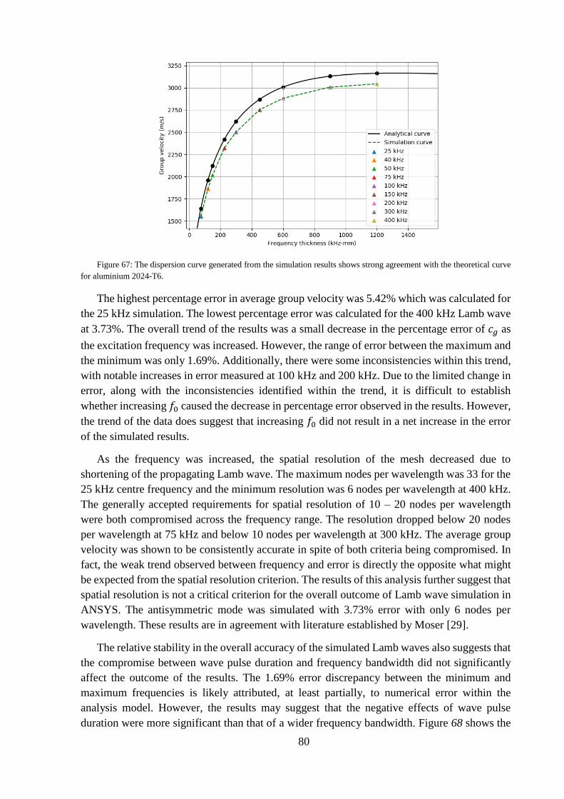
80
Figure 67: The dispersion curve generated from the simulation results shows strong agreement with the theoretical curve
for aluminium 2024-T6.
The highest percentage error in average group velocity was 5.42% which was calculated for
the 25 kHz simulation. The lowest percentage error was calculated for the 400 kHz Lamb wave
at 3.73%. The overall trend of the results was a small decrease in the percentage error of 𝑐𝑔 as
the excitation frequency was increased. However, the range of error between the maximum and
the minimum was only 1.69%. Additionally, there were some inconsistencies within this trend,
with notable increases in error measured at 100 kHz and 200 kHz. Due to the limited change in
error, along with the inconsistencies identified within the trend, it is difficult to establish
whether increasing 𝑓0 caused the decrease in percentage error observed in the results. However,
the trend of the data does suggest that increasing 𝑓0 did not result in a net increase in the error
of the simulated results.
As the frequency was increased, the spatial resolution of the mesh decreased due to
shortening of the propagating Lamb wave. The maximum nodes per wavelength was 33 for the
25 kHz centre frequency and the minimum resolution was 6 nodes per wavelength at 400 kHz.
The generally accepted requirements for spatial resolution of 10 – 20 nodes per wavelength
were both compromised across the frequency range. The resolution dropped below 20 nodes
per wavelength at 75 kHz and below 10 nodes per wavelength at 300 kHz. The average group
velocity was shown to be consistently accurate in spite of both criteria being compromised. In
fact, the weak trend observed between frequency and error is directly the opposite what might
be expected from the spatial resolution criterion. The results of this analysis further suggest that
spatial resolution is not a critical criterion for the overall outcome of Lamb wave simulation in
ANSYS. The antisymmetric mode was simulated with 3.73% error with only 6 nodes per
wavelength. These results are in agreement with literature established by Moser [29].
The relative stability in the overall accuracy of the simulated Lamb waves also suggests that
the compromise between wave pulse duration and frequency bandwidth did not significantly
affect the outcome of the results. The 1.69% error discrepancy between the minimum and
maximum frequencies is likely attributed, at least partially, to numerical error within the
analysis model. However, the results may suggest that the negative effects of wave pulse
duration were more significant than that of a wider frequency bandwidth. Figure 68 shows the

81
25 kHz and 400 kHz raw mesh node results at 120 mm from the excitation source. Here it can
be seen that the increased pulse duration for the 25 kHz excitation results in less separation
between the incident and reflected wave pulses. While the analysis methodology did take the
reflected wave pulses into account, it is possible that some numerical error was introduced into
the model as a result of the boundary reflections.
a) b)
Figure 68: The increased wave duration for the 25 kHz model resulted in less separation between incident and reflected
wave pulses (a), which may have introduced numerical error not seen in higher frequency models such as 400 kHz (b).
Figure 68 also demonstrates the difference in displacement amplitude captured between the
25 kHz and 400 kHz simulations. To investigate the relationship between amplitude and
frequency, the maximum displacement at 𝑥 = 10 𝑚𝑚 was recorded for each of the simulations.
The displacement data was then graphed as a function of frequency by Figure 69. The trend of
the data demonstrates a clear relationship between excitation frequency and nodal displacement
amplitude. The effect of increasing frequency of the excitation, whilst keeping the amplitude
fixed, is a reduction in the amplitude of the propagating Lamb wave. This is an important
consideration in SHM practices, as the detection of wave pulses can be limited by the resolution
of the transducer. Hence, it should be understood that increasing frequency of the excitation
will reduce the overall amplitude of the measured response. This relationship should be
considered when designing SHM systems to ensure that the sensors are compatible with the
relative amplitude of the signal response.
Figure 69: Increasing excitation frequency resulted in reduced displacement amplitude.
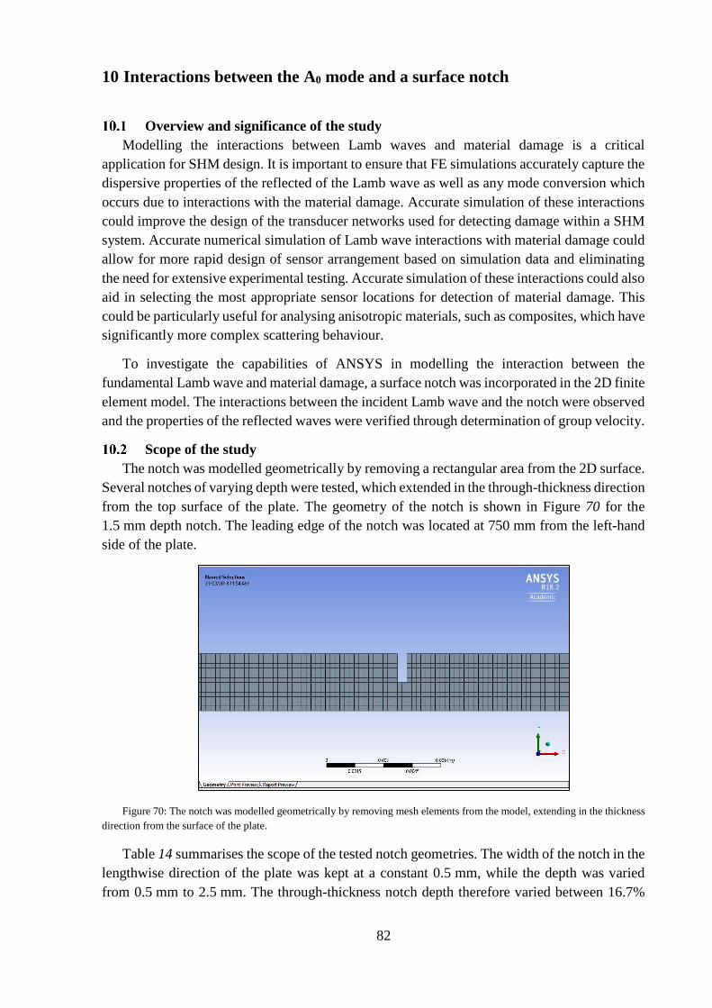
82
10 Interactions between the A0 mode and a surface notch
Overview and significance of the study
Modelling the interactions between Lamb waves and material damage is a critical
application for SHM design. It is important to ensure that FE simulations accurately capture the
dispersive properties of the reflected of the Lamb wave as well as any mode conversion which
occurs due to interactions with the material damage. Accurate simulation of these interactions
could improve the design of the transducer networks used for detecting damage within a SHM
system. Accurate numerical simulation of Lamb wave interactions with material damage could
allow for more rapid design of sensor arrangement based on simulation data and eliminating
the need for extensive experimental testing. Accurate simulation of these interactions could also
aid in selecting the most appropriate sensor locations for detection of material damage. This
could be particularly useful for analysing anisotropic materials, such as composites, which have
significantly more complex scattering behaviour.
To investigate the capabilities of ANSYS in modelling the interaction between the
fundamental Lamb wave and material damage, a surface notch was incorporated in the 2D finite
element model. The interactions between the incident Lamb wave and the notch were observed
and the properties of the reflected waves were verified through determination of group velocity.
Scope of the study
The notch was modelled geometrically by removing a rectangular area from the 2D surface.
Several notches of varying depth were tested, which extended in the through-thickness direction
from the top surface of the plate. The geometry of the notch is shown in Figure 70 for the
1.5 mm depth notch. The leading edge of the notch was located at 750 mm from the left-hand
side of the plate.
Figure 70: The notch was modelled geometrically by removing mesh elements from the model, extending in the thickness
direction from the surface of the plate.
Table 14 summarises the scope of the tested notch geometries. The width of the notch in the
lengthwise direction of the plate was kept at a constant 0.5 mm, while the depth was varied
from 0.5 mm to 2.5 mm. The through-thickness notch depth therefore varied between 16.7%

83
and 83.3% relative to the 3 mm thick plate. The depth of the notch was varied to investigate the
influence of notch depth on the amplitude of the reflected Lamb waves.
Table 14: Summary of tested notch geometries.
Notch width (mm) Notch depth (mm) Through thickness depth (%)
0.5 0.5 16.7
0.5 1.0 33.3
0.5 1.5 50.0
0.5 2.0 66.7
0.5 2.5 83.3
The model was meshed using 4-node solid elements with a characteristic mesh element
length of 0.25 mm. The analysis was performed using the 2D model to reduce computational
complexity as well as to simplify the modelling of the notch. The mesh element length was
selected at 0.25 mm based on the acceptable compromise between computation speed and
model accuracy seen in section 6.4.6. A 0.25 mm mesh element length also provided an
adequate resolution to model the tested notch depths.
The excitation frequency was selected at 100 kHz and the plate properties were for
aluminium 2024-T6. This allowed for a direct comparison between the results captured from
the damaged plate and those captured from the undamaged plate in section 6.4.6.
Results
The simulations were carried out for the various notch depths and the results were extracted
from ANSYS for analysis. The ANSYS graphical output of the nodal displacement data clearly
shows that interaction between the incident wave pulse and the surface notch results in a
reflected wave pulse in the direction of the excitation source. This is shown for the 1.5 mm deep
notch in Figure 71.
Figure 71: Interaction between the incident Lamb wave and the surface notch resulted in a reflected wave propagating
back toward the excitation source.
Magnification of the nodal displacement results captured at 𝑥 = 210 𝑚𝑚 reveals a
symmetric wave reflected from the notch. This is shown in Figure 72 below. The wave pulse
was hypothesised to be the fundamental S0 mode generated through mode conversion due to
interactions with the notch. This hypothesis was to be confirmed through comparison of the
group velocity with the theoretical wave speed of the S0 mode. Arrival of the symmetric mode
Reflected wave pulse Incident wave pulse

84
was indicated by the distinct pattern of alternating ‘thick’ and ‘thin’ pulses which were
discussed in the literature (see Figure 1 (a)). The amplitude of the symmetric Lamb mode was
significantly lower in magnitude than the antisymmetric mode. Because of the large difference
in amplitude, the scale used in Figure 71 was insufficient to see the S0 mode. The symmetric
mode was also observed to arrive earlier than the antisymmetric mode. This indicated the wave
pulse travelled with a higher group velocity, which is consistent with the dispersive properties
of aluminium 2024-T6 (see Figure 3 (b)).
Figure 72: The nodal displacement response at 210 mm from the excitation source reveals the symmetric Lamb mode is
reflected from the notch and arrives earlier than the A0 mode.
The results captured at 𝑥 = 210 𝑚𝑚 also reveal the antisymmetric mode reflected from the
notch, as seen in Figure 73. The A0 mode was observed to arrive later than the S0 mode.
Figure 73: The nodal displacement response at 210 mm from the excitation source reveals the antisymmetric Lamb mode
is reflected from the notch and arrives later than the S0 mode.
Analysis of the nodal displacement data
Both x and y nodal displacements were captured in the ANSYS simulation and the data was
exported for quantitative analysis in Python. Nodal displacements in the y direction were
measured to capture the out-of-plane motion of the antisymmetric mode. The x direction nodal
displacement was measured to capture the symmetric mode, which primarily induces in-plane
motion. Figure 74 presents the y displacement data captured at 300 mm from the excitation
Reflected S0 mode
Reflected A0 mode

85
source, when the notch depth was 1.5 mm. The Hilbert transform of the signal provides the
energy envelope of the wave pulses, presented in Figure 75.
Figure 74: The y direction nodal displacement at 300 mm from the excitation source reveals the wave pulses reflected off
the structural damage, along with significant boundary noise.
The notable features within the captured nodal displacement dataset are labelled on each of
the plots. The incident A0 wave pulse was captured at approximately 152 𝜇𝑠 by the measured
mesh node at 300 mm from the excitation source. Interaction between the incident Lamb wave
and the 1.5 mm notch results in wave pulses reflected from the damage back in the direction of
the excitation source. The small peak indicating the reflected S0 Lamb wave can be identified
from Figure 75, occurring at 391 𝜇𝑠. The reflected A0 wave is more clearly identified in the
nodal displacement data as a result of its larger amplitude, with the approximate ToA at 485 𝜇𝑠.
The displacement of the A0 wave is larger in amplitude as it causes predominantly out-of-plane
nodal displacement, while the S0 mode is primarily in plane displacement. The remainder of the
captured signal is dominated by noise resulting from boundary reflections both from the
incident Lamb wave reflecting off the far boundary and the scattered wave reflecting off the
excitation boundary. The noise within this region demonstrates the difficulties which can be
experienced when analysing the nodal displacement data due to reflections off system
boundaries and other discontinuities. Careful attention must be maintained to ensure that the
correct amplitude peak for the scattered wave pulse is identified among the noise of the
measured data.
Incident wave pulse
Reflected S0 mode
Reflected A0 mode
Boundary reflections

86
Figure 75: The Hilbert transform of the y direction nodal displacement data was used to distinguish the reflected wave
pulses and determine ToA.
Figure 76 (a) and (b) present a comparison of the results between the damaged and
undamaged 2D plate models. The nodal displacement data in the y direction is plotted for each
scenario and helps to confirm the nature of the identified wave peaks. The incident Lamb wave
and the wave pulse reflected off the far boundary of the plate appear in the results of undamaged
plate, while the identified A0 and S0 modes scattered by the surface notch do not. This confirms
that the source of these wave peaks was indeed the interaction between the incident wave and
the material damage.
a) b)
Figure 76: Comparison of the y displacement data between the damaged and undamaged plate confirms the nature of the
wave peaks as the reflected A0 and S0 modes only appear due to interaction with the notch.
Close-up views of the reflected wave pulses are shown in Figure 77 (a) and (b) below. Since
Figure 77 plots the out-of-plane displacement, the amplitude of the reflected A0 mode is much
larger than the in-plane S0 mode. The times of arrival of the reflected wave pulses were
approximated using the wave pulse energy envelope method. The amplitude threshold over
which time was averaged was defined at 90% of the local maximum. The average ToA of the
Incident wave pulse
Reflected S0 mode
Reflected A0 mode
Boundary reflections

87
reflected S0 mode was approximately 391 𝜇𝑠, while the A0 mode was approximately 485 𝜇𝑠.
The approximate locations are marked in Figure 77 (b).
a) b)
Figure 77: Closeup view of the y displacement data shows the S0 mode is detected earlier than the A0 mode as the
symmetric mode travels at a higher group velocity, as indicated in the aluminum 2024-T6 dispersion curves.
The nodal displacement in the x direction, measured 300 mm from the excitation, is plotted
in Figure 78, along with the Hilbert transform of the signal in Figure 79. The plots present data
captured in the 1.5 mm notch simulation. The incident and reflected S0 wave modes are more
clearly discernible due to capturing the in-plane (x direction) nodal displacement. Observing
the incident wave pulses, it can be identified that the S0 mode arrives earlier than the A0 mode.
This is due to the S0 mode’s higher group velocity at 5385 m/s compared with the A0 mode
(2621 m/s) at a frequency thickness of 300 kHz-mm (see Figure 3 (b)). The antisymmetric mode
maintains a larger amplitude than the S0 mode in the x direction due to the out-of-plane nature
of the excitation nodal displacement. The excitation perturbation was specifically selected in
the through-thickness direction (y) to excite primarily the A0 mode. Hence, the S0 wave pulse
which is generated in the process has a significantly smaller amplitude.
Note, it can be observed from Figure 78 that there are two reflected S0 wave pulses in the
signal response. The first mode, observed at 230 𝜇𝑠, is the reflection produced when the
incident S0 mode encountered the material damage. The amplitude of this wave pulse is
comparatively low due to the out-of-plane excitation producing a low-energy incident S0 mode.
The second S0 wave pulse has a significantly larger amplitude and arrived later at 391 𝜇𝑠. This
is because this S0 mode was produced due to mode conversion when the A0 mode encountered
the material damage. Since this investigation focused primarily on the A0 Lamb mode, further
reference to the reflected S0 mode is specific to the wave pulse produced by mode conversion.
This is discussed in further detail below.
Reflected S0 mode
Reflected A0 mode Reflected S0 mode
Reflected A0 mode

88
Figure 78: Measurement of the x direction nodal displacements improves detection of the incident and reflected symmetric
Lamb modes.
The reflected S0 and A0 modes are indicated in Figure 79. The relative amplitude of the S0
mode is significantly pronounced than that seen in Figure 75. This makes determination of ToA
for the symmetric mode significantly more convenient and accurate using the energy envelope
method.
Figure 79: The energy envelope of the x direction nodal displacement data provides enhanced identification of the
symmetric mode and was used to calculate group velocity.
Figure 80 compares the nodal displacement data recorded in the undamaged plate and the
damaged plate (1.5 mm notch depth). The normalised displacement data are presented in (a)
from which the S0 and A0 wave pulses reflected from the material damage are clearly
distinguishable from the boundary reflections. Comparison with the undamaged plate reveals
Incident A0 mode
Reflected S0 mode
Reflected A0 mode
Boundary reflections
Incident S0 mode
Reflected S0 mode
Incident A0 mode
Reflected S0 mode
Reflected A0 mode
Boundary reflections
Incident S0 mode
Reflected S0 mode

89
the nature of the low amplitude wave pulses measured at 335 𝜇𝑠 and 458 𝜇𝑠. The first wave
pulse (1) is the reflection of the incident S0 pulse from the far boundary, while (2) is the second
reflection off the boundary located at the excitation origin. Due to its significantly higher
velocity, the S0 mode reflections occur prior to the arrival of the A0 mode at 663 𝜇𝑠 (3). These
wave peaks are labelled on the energy envelope plot provided in (b).
a) b)
Figure 80: The x direction nodal displacement data was used to distinguish the structural damage reflections from the
boundary reflections (a). The boundary reflections are clearly identified from the undamaged plate (b).
Closeup views of the reflected A0 and S0 wave pulses are provided in Figure 81. Through
measurement of the x nodal displacement the S0 mode amplitude is more clearly discernible
from the signal response. The times of arrival of the reflected S0 and A0 wave pulses were
determined at 386 𝜇𝑠 and 485 𝜇𝑠 respectively using the nodal y displacement data.
Observation of (b) confirms that the same results are yielded from the x nodal data, which
supports the methodology as the two datasets agree.
a) b)
Figure 81: The reflected A0 and S0 wave pulses (a) were distinguished from the boundary noise by comparison of the x
direction signal response with that captured for the undamaged plate (b).
The x and y nodal displacement results are provided in Figure 82 (a) and (b) respectively,
centred around the reflected wave pulses. The reflected S0 and A0 Lamb wave pulses are labelled
in Figure 82 (a). Comparison between the two plots reveals the large change in relative
amplitude of the S0 mode depending on the axis of displacement measured by the analysis. The
S0 mode is almost unable to be discerned in (b) while it is clearly identifiable in (a). The A0
(1)
(2)
(3)
Reflected A0 mode
Reflected S0 mode
Reflected A0 mode
Reflected S0 mode

90
mode has a significant amplitude in both plots as the excitation signal was an out-of-plane
displacement, hence exciting primarily the A0 mode.
Analysis of the plots also reveals the mode conversion between the A0 mode and the S0
mode, which occurred after interaction with the surface notch. Mode conversion occurs when
Lamb waves encounter a discontinuity [2, 5]. The interaction results in scattering of the
longitudinal (P) and shear waves (SV) waves, which interfere constructively and destructively
to form reflected A0 and S0 modes [11]. The mode conversion identifiable within the ANSYS
simulation data is highly consistent with results obtained by published authors (see below).
a) b)
Figure 82: Mode conversion is clearly evident between the antisymmetric and symmetric modes through measurement
of x displacement (a). The A0 amplitude is much greater than that of the S0 mode in the y direction, due to the out-of-plane
perturbation (b).
Alkassar investigated the propagation of the A0 mode and interactions with a surface crack
extending vertically from the surface of the plate [10]. Alkassar published Figure 83 (a) which
shows the captured x direction nodal displacements, showing the mode conversion between the
A0 and the S0 mode after encountering a crack [10]. Comparison between Figure 82 (a) and
Figure 83 (a) yield strong agreement between the behaviour of the Lamb wave after interaction
with damage. Mode conversion was observed in both cases after interaction with damage.
Additionally, the amplitude of the A0 is greater than the S0 mode in the x direction in both cases
as both involved excitation perturbations in the through-thickness direction.
Su discussed the mode conversion that occurs when Lamb waves interact with structural
damage [2]. Figure 83 (b) provides results published by Su, showing the mode conversion
between the S0 and A0 modes after interaction with damage [2]. The mode conversion shows
strong agreement with the results obtained in this investigation.
The agreement between the simulation results and the findings published in literature
provide evidence of the reliability of the data produced in the ANSYS simulation. Mode
conversion was captured after the Lamb wave encountered the notch. To provide a quantitative
validation of the reflected wave pulses, the group velocities were to be determined.
Mode conversion
S0 A0

91
a) b)
Figure 83: Simulation results published by Alkassar (a), capturing the x direction nodal displacement after the A0 Lamb
wave interaction with a vertical surface crack [10]. Results published by Su (b), showing mode conversion between the S0
and A0 modes after interaction with structural damage [2].
To quantitatively validate the reflected S0 and A0 Lamb wave pulses, the group velocities
were calculated using the energy envelope approach for ToA. The nodal separation was 90 mm
and the amplitude threshold for ToA was 90% to remain consistent with previous analyses.
Figure 84 demonstrates how the group velocities of the reflected S0 and A0 wave pulses were
determined. The A0 wave pulse is shown at two locations, (a) 180 mm and (b) 270 mm from
the excitation. The group velocity of the A0 wave pulse is therefore 2647 m/s as shown below.
Similarly, the S0 wave pulse is shown at (c) 180 mm and (d) 270 mm, with the corresponding
group velocity calculated at 5294 m/s. The average wave pulse group velocity was calculated
by averaging the calculated 𝑐𝑔 across all measured mesh nodes. The complete datasets of ToA
and corresponding group velocities are provided in Appendix D (see 15.4).
𝑐𝑔, 𝐴0=
270 − 180
532 − 498𝑚/𝑠 = 2647 𝑚/𝑠 𝑐𝑔, 𝑆0
=270 − 180
414 − 397𝑚/𝑠 = 5294 𝑚/𝑠
a) 𝑇𝑜𝐴 = 532 𝜇𝑠 b) 𝑇𝑜𝐴 = 498 𝜇𝑠

92
c) 𝑇𝑜𝐴 = 414 𝜇𝑠 d) 𝑇𝑜𝐴 = 397 𝜇𝑠
Figure 84: The ToA of the reflected S0 and A0 wave pulses were determined, and the corresponding group velocities
were calculated. The range of data was averaged to determine the average group velocity.
The average group velocity of the reflected A0 wave pulse was calculated at 2583 m/s.
Compared with the theoretical wave speed of 2621 m/s, the error in the calculated results is
approximately 1.44%. Note, the incident A0 wave speed was calculated in the undamaged plate
at 2587 m/s. Comparison between incident and reflected waves reveals a slight drop in group
velocity. The scale of the velocity decrease is within the margins of numerical error, but may
also be due to energy losses in the wave pulse after interaction with the notch. This would occur
due to the scattering and reforming of the A0 mode after encountering the damage. The wave
speed may also have decreased due to the effects of attenuation, primarily energy leakage to
the surrounding environment or due to frictional losses. Overall, the reflected A0 mode is highly
consistent with the theoretical wave speed and previously calculated results.
The group velocity of the S0 pulse reflected from the surface notch was calculated at
5321 m/s. The theoretical group velocity at 300 kHz-mm was approximately 5385 m/s. The
percentage error associated with the calculated value was therefore only 1.18%. This low error
suggests the simulated mode conversion of the A0 mode to the S0 mode, which took place after
the incident wave encountered the material damage, was highly accurate. This analysis also
provides evidence of the capabilities of ANSYS in modelling the S0 Lamb mode with a high
degree of accuracy.
The calculated group velocities of the reflected A0 and S0 modes evidences the capabilities
of ANSYS in accurately modelling the interactions between the A0 Lamb wave and material
damage. The simulation accurately modelled the complex mode conversion which occurs due
to wave scattering and reformation after interaction with a discontinuity. The interactions
between the incident Lamb wave and the surface notch, including mode conversion and wave
pulse reflection, were found to be consistent with results published within the literature. The
group velocities of the reflected Lamb waves were found to strongly agree with the theoretical
wave speeds determined from the dispersion curves for aluminium 2024-T6.
Influence of notch depth on the amplitude of reflected Lamb waves
Being able to identify and determine the nature of damage within a component is integral
to applications of NDT in structural health monitoring. To determine if there was a relationship
between notch depth and the nature of the reflected Lamb wave pulses, simulations were carried
out using the various geometries provided in Table 14. The notch depth was varied between

93
0.5 mm (16.7% plate thickness) and 2.5 mm (83.3% plate thickness). Both the x and y nodal
displacements were measured to capture the reflected S0 and A0 Lamb wave pulses. The data
was then exported and plotted for subsequent analysis.
The in-plane (x) nodal displacements at 120 mm, 210 mm, 330 mm and 420 mm from the
excitation source are plotted in Figure 85 (a), (b), (c) and (d) respectively. The plots capture the
S0 mode (labelled) produced due to mode conversion when the A0 mode interacted with the
material damage at the various notch depths. At all measured points along the plate, the
amplitude of the reflected S0 mode was found to increase as the notch depth was increased. The
greatest amplitude of the reflected S0 mode occurred for the 2.5 mm notch and the smallest
amplitude occurred for the 0.5 mm notch. The trend is more inconsistent for the A0 mode, which
saw the largest amplitude for a number of notch depths, depending on where the point of
reference was taken. For this reason, the x direction nodal displacement was not considered a
reliable source for establishing a trend for the A0 mode.
a) b)
c) d)
Figure 85: The x direction nodal displacement data indicates that increased notch depth resulted in larger amplitude of
the reflected S0 Lamb wave pulse, measured at (a) 120 mm, (b) 210 mm, (c) 330 mm, (d) 420 mm.
The out-of-plane (y) nodal displacements at 120 mm, 210 mm, 330 mm and 420 mm from
the excitation source are plotted in Figure 86 (a), (b), (c) and (d) respectively. Measurement of
the y direction nodal displacement suggests a more consistent trend in the reflected A0 wave
pulse response than the in-plane displacement data. In all measured nodal responses, the 1.5 mm
notch (50% plate depth) was found to cause the largest amplitude of the reflected A0 wave pulse.
S0
A0
S0 A0
S0 A0 S0
A0

94
The 2 mm notch induced the second largest amplitude response, followed by the 1.0 mm and
2.5 mm notches, which produced similar responses. The 0.5 mm notch was found to induce a
reflected A0 Lamb wave with the smallest relative amplitude of all tested notch sizes. Notably,
the trend observed in the x nodal displacement for the S0 mode holds true for the y displacement
data. Increased notch depth consistently resulted in a reflected S0 wave pulse with a larger
relative amplitude.
a) b)
c) d)
Figure 86: The y direction nodal displacement data indicates that a mid-thickness notch depth results in the largest
amplitude of the reflected A0 Lamb wave pulse, measured at (a) 120 mm, (b) 210 mm, (c) 330 mm, (d) 420 mm.
The results provided in Figure 85 suggest that the relative depths of multiple surface notches
could be predicted based on the amplitude response of the reflected S0 mode, measured in the x
direction. The trend of the data suggests that increasing notch depth consistently results in a
larger amplitude of the reflected S0 wave pulse. Due to inconsistent trends between x and y
nodal displacements, the x displacement data was found to be unreliable for the A0 mode.
The data presented in Figure 86 suggests that the maximum amplitude of the reflected A0
wave mode occurs for mid-thickness notch depths. The amplitude response was seen to
decrease (on average) as the notch depth tended away from the depth-to-thickness ratio of 0.5.
The out-of-plane nodal displacement data showed a consistent trend in S0 amplitude as was
observed from the in-plane displacement data presented in Figure 85.
A0
S0
A0
S0
A0
S0
A0
S0

95
This investigation highlights the fact that careful attention must be paid when interpreting
the amplitude response of damage-reflected Lamb waves. Depending on the direction of
displacement which is measured, different trends were established. The results suggested that
the amplitude of the S0 mode provides a consistent trend of increasing amplitude with notch
depth when both in-plane and out-of-plane displacement are measured. However, the same
consistency was not seen for the A0 mode, which showed no consistent trend for in-plane
displacement, while out-of-plane displacement suggested a mid-thickness notch depth causes
the largest amplitude response.
The scope of the tested notch depths was limited by time constraints, which meant that the
observations made in this study could not be evidenced more rigorously. There is insufficient
data to conclusively show that the relationship between amplitude and notch depth is generally
true. Hence it is recommended that future works focus on this relationship in order to validate
the observations made in this study. These works may use a more incremental variation in notch
geometry and a range of frequencies to investigate whether the trends observed in this report
hold true in a general sense.
11 Interactions between the A0 mode and a mid-thickness void
Overview of the study
The capabilities of ANSYS in modelling the interaction with a notch have been investigated,
with high levels of agreement between literature and analytical results. To extend the relevance
of the conclusions, the model was modified to incorporate a horizontal void at the centre of the
plate. The interaction between the incident A0 Lamb wave and the material damage was to be
analysed and the results compared with the established literature.
Scope of the study
A rectangular void was modelled in the centre of the plate, located at 750 mm from the
excitation source. The thickness of the void was 0.5 mm and the length was varied between
1 mm and 30 mm (see Table 15). Figure 87 shows the horizontal void when the length was
5 mm. The model was meshed with 4-node solid elements and the material properties were that
of aluminium 2024-T6. The characteristic mesh element length remained at 0.25 mm, as this
resolution provided sufficient numerical accuracy whilst also resulting in simulations fast
enough to allow for the numerous test cases. The excitation frequency remained at 100 kHz and
the signal was a 5-cycle sinusoidal tone burst modified with a Hanning window function.

96
Figure 87: A horizontal void was modelled in the centre of the plate, with varying lengths ranging between 1 – 30 mm.
Table 15 summarises the scope of the testing, including the geometries of the tested damages
along with their relative sizes compared with the theoretical A0 wavelength at a central
frequency of 100 kHz (15.5 mm).
Table 15: Summary of the tested void lengths.
Void thickness (mm) Void length (mm) Length relative to A0 wavelength (%)
0.5 1 6.5
0.5 1.5 9.7
0.5 2 12.9
0.5 3 19.4
0.5 4 25.8
0.5 5 32.3
0.5 7.5 48.4
0.5 10 64.5
0.5 15 96.8
0.5 20 129.0
0.5 30 193.5
Model results
The simulation results revealed a reflected A0 wave pulse was produced during the
interaction between the incident A0 Lamb wave and the void located in the centre of the
aluminium plate. The reflected antisymmetric mode is clearly visible in Figure 88 which shows
the simulation results for the 5 mm void. Upon closer inspection of the results, there was no
evidence of a reflected S0 wave being produced as a consequence of the interaction between the
incident wave and the material damage. This type of interaction was seen between the incident
Lamb wave and the surface notch. To investigate this observation more rigorously, both the x
and y nodal displacements were exported from the model and the results were analysed in
Python.

97
Figure 88: The ANSYS simulation results reveal only the A0 Lamb mode was reflected from the material damage.
Analysis of the nodal displacement data
The normalised in-plane nodal displacement captured during the simulation of the 5 mm
length void is shown by Figure 89 (a) and the corresponding energy envelope of the data in (b).
The nodal data was captured at 210 mm from the excitation source. The displacement data for
the undamaged plate is also graphed to aid in distinguishing the damage-reflected wave pulses
from the incident and boundary-reflected wave pulses. Comparison between the damaged and
undamaged nodal data reveals that only one reflected wave pulse was produced by interaction
with the horizontal crack. This wave pulse was the A0 mode reflected from the material damage,
with a ToA of approximately 510 𝜇𝑠. The S0 wave pulses observed within the simulation data
(occurring at 69 𝜇𝑠, 352 𝜇𝑠, and 442 𝜇𝑠) were observed in both the damaged and undamaged
plates. Hence, these wave pulses were incident and boundary-reflected, and were not
consequences of interactions with the material damage.
a)
Reflected A0 wave pulse Incident A0 wave pulse

98
b)
Figure 89: The normalised x directional nodal displacement data (a) and corresponding energy envelope (b) at 210 mm
reveals a damage-reflected A0 mode. No S0 mode was generated due to interaction with 5 mm long damage.
The out-of-plane nodal displacement data at 210 mm from the excitation source, for the 5 mm
horizontal void, is shown in Figure 90 (a), with the energy envelope of the data presented in
(b). The nodal results clearly show the same reflected A0 Lamb wave at 510 𝜇𝑠 as seen in the x
nodal data. The wave pulse was produced as a consequence of interactions between the incident
A0 Lamb wave and the horizontal void located at 750 mm.
Notably, all tested void lengths produced similar displacement results, with only the A0 mode
being reflected from the material damage. The group velocity of the reflected Lamb wave was
calculated by measuring the ToA at various points along the plate and using the separation
distance between nodes to determine 𝑐𝑔. The average group velocity of the reflected A0 Lamb
wave due to interaction with the 5 mm void was 2571 m/s, thus a 1.89% error compared with
the theoretical wave speed. The high level of agreement between the reflected Lamb wave
group velocity and the analytical wave speed validates the accuracy of the simulation in a
quantitative sense. The reflected wave pulse produced due to interactions between the A0 Lamb
wave and the horizontal void was accurately simulated by the ANSYS Explicit Dynamics
solver, with a physically realistic wave speed consistent with analytical results.
a)

99
b)
Figure 90: The normalised y directional nodal displacement data (a) and corresponding energy envelope (b) at 210 mm
clearly shows the reflected A0 mode from the 5 mm long centrally located void.
Figure 91 provides a closeup view of the x direction nodal displacement data captured at
210 mm from the excitation source. The nodal displacement data (a) and energy envelope (b)
reveals the A0 mode reflected from the 5 mm void, and the S0 modes appearing in both the
damaged and undamaged plate. It is clear from the results that no significant mode conversion
took place between the A0 mode and S0 mode due to interaction with the material damage. This
is because the void was located in the centre of the plate, at which the shear stress is zero. As
discussed in the literature, Guo and Cawley determined the S0 mode was not capable of
detecting delaminations at through-thickness locations with zero shear stress [9]. Figure 92
presents the distribution of shear stress through the thickness of the 3 mm plate, generated using
the software package Disperse. The plot shows that the shear stress is minimized at the centre
and surfaces of the plate. Thus, as the void was located at the mid-thickness of the plate, the
shear stress at the damage was zero. This explains why the S0 mode was not produced as a
consequence of the interaction of the wave pulse with the damage. The simulation results
therefore agree with the established literature and evidence the capabilities of ANSYS Explicit
Dynamics in accurately modelling interactions between Lamb waves and material damage.
a) b)
Figure 91: In-plane (x) displacement at 240 mm reveals no mode conversion between the A0 and S0 modes as a result of
interaction with the 5 mm void. This is because the void is located in the centre of the plate where the shear stress is zero.

100
Figure 92: Stress data generated using the software Disperse shows the shear stress distribution across the thickness of the
plate, with the shear stress being zero at the centre.
A closeup view of the out-of-plane nodal displacement data is shown in Figure 93 centred
around the reflected A0 Lamb wave. Here it can be seen that the presence of the horizontal void
in the mid-plane of the plate resulted in a reflection of the A0 mode, with no significant mode
conversion to the S0 mode. The findings suggest that detection of a reflected A0 pulse, when the
incident Lamb wave is the A0 mode, may be used to characterise material damage occurring in
the midplane of the plate.
a) b)
Figure 93: Out-of-plane (y) displacement at 240 mm shows the A0 wave pulse reflected off the 5 mm horizontal void.
The wave pulse has an approximate ToA of 500 𝜇𝑠.
Influence of void length on the amplitude of the reflected Lamb wave
The length of the void was varied between 1 mm and 30 mm to investigate the influence of
damage length on the received A0 Lamb wave. The full range of damage geometries are
provided in Table 15. The results were graphed in two distinct datasets, those with a damage
length of 1 – 5 mm and those with damage length of 5 – 30 mm. The differences between these
datasets is discussed in the analysis below.
The out-of-plane nodal displacement data was captured at four locations along the plate;
120 mm, 210 mm, 330 mm, 420 mm from the excitation source. The energy distribution of each

101
amplitude response was then calculated, and the results were plotted in Figure 94 (a), (b), (c)
and (d). Figure 94 provides the amplitude response captured for the models containing void
lengths of 1 – 5 mm, centred at the damage-reflected A0 Lamb wave. A consistent trend was
observed across all captured mesh nodes (including those presented in Figure 94). It is clear
from the energy distribution results that increasing the length of the horizontal void resulted in
increasing amplitude of the reflected A0 Lamb wave. The largest relative amplitude of the
damage-reflected Lamb wave was seen in the 5 mm damage, while the smallest relative
amplitude was seen for the 1 mm void. As can be seen from the plots, the time of arrival of the
reflected A0 Lamb wave was consistent across void lengths of 1 – 5 mm.
a) b)
c) d)
Figure 94: The y direction nodal displacement data indicates that increased void length (up to 5 mm) resulted in larger
amplitude of the reflected A0 Lamb wave pulse, measured at (a) 120 mm, (b) 210 mm, (c) 330 mm, (d) 420 mm.
The energy distribution results for void lengths of 5 – 30 mm are provided in Figure 95 at
(a) 120 mm, (b) 210 mm, (c) 330 mm, (d) 420 mm from the excitation source. The
aforementioned trend between void length and the amplitude of the reflected A0 mode was not
discernible within this range. In this case, the largest amplitude occurred for the 5 mm void,
followed by the 15 mm void, while the 7.5 mm and 20 mm voids showed similar amplitude
response. Finally, the 10 mm and 30 mm void lengths resulted in the smallest relative amplitude
responses, with the latter case producing almost no discernible reflected wave pulse.
A0 A0
A0 A0

102
a) b)
c) d)
Figure 95: The y direction nodal displacement data reveals the relationship breaks down at void lengths larger than 5 mm,
measured at (a) 120 mm, (b) 210 mm, (c) 330 mm, (d) 420 mm. No discernible trend was identified between amplitude and
void lengths from 5 – 30 mm.
The relationship between void length and the reflected A0 Lamb wave amplitude was found
to be variable across the range of tested geometries (1 – 30 mm). However, a clear trend was
observed within the range of 1 – 5 mm, with increasing length resulting in a larger amplitude
of the reflected A0 Lamb wave. The results of the testing suggest that the amplitude of the
reflected A0 wave could be used to characterise the size of the material damage, within the range
of 1 - 5 mm (when the excitation frequency is 100 kHz). It is hypothesised that the ratio between
wavelength and void length may be a factor in the stability of this trend, as the relationship was
observed to break down when the damage size exceeded 32.3% of the wavelength. When the
length of the void increased above 32.3% of the central excitation wavelength (greater than
5 mm), the amplitude of the reflected A0 Lamb wave did not show any discernible relationship
with damage size.
Due to time constraints, the scope of the tested void length range was relatively limited.
There were insufficient data points collected within this study to conclusively validate the
trends observed between void length and wavelength. Hence, it is recommended that further
studies are carried out using a more sensitive incremental variation in notch length to validate
the hypothesis. The testing should involve a range of frequencies to confirm if the relationship
between void length and amplitude holds true across the frequency spectrum.
A0
A0
A0 A0

103
12 Recommendations for further works
ANSYS Explicit Dynamics was proven highly capable of modelling the A0 Lamb mode in
aluminium 2024-T6. The simulation results were validated against theoretical wave properties
and ANSYS was shown to be a viable tool for both 2D and 3D analyses. ANSYS is therefore
recommended in future works which focus on Lamb wave-based SHM systems. The
methodology outlined in this report could be used as a reference for simulating the A0 mode in
ANSYS. Through providing a validated methodology for simulating the A0 mode in ANSYS,
this thesis has opened a range of further works to explore. The topics discussed below are
mainly based on elements which were either out of the scope of this investigation due to time
constraints, or aim to extend upon particular observations made throughout the investigation.
Structural health monitoring systems are highly attractive for composite materials as they
exhibit more complicated damage modes than conventional materials. A valuable extension to
the work carried out in this investigation would be the development of a 3D composite laminate
in ANSYS. The propagation and scattering characteristics of the A0 Lamb wave could then be
explored. Due to time and resource constraints the scope of this investigation was limited to
isotropic material properties. However, the behaviour of Lamb waves in anisotropic materials
such as composites can be significantly more complex. Hence, this research extension would
provide further validation of the capabilities of ANSYS in modelling more complex behaviour.
Development of a viable numerical tool for modelling the propagation of Lamb waves in a
composite material could be highly useful in design of SHM systems. Ng and Veidt modelled
the A0 mode in a carbon-epoxy laminate using LS-DYNA [8]. This research is recommended
as a starting point for future investigations carried out in ANSYS Explicit Dynamics.
Figure 96: Ng and Veidt modelled the propagation of the A0 mode in a composite laminate using ANSYS LS-DYNA.
Development of a 3D composite model in ANSYS Explicit Dynamics could provide a viable tool for SHM system design [8].
This investigation involved the interaction between the A0 mode and a surface notch. The
amplitude of the reflected S0 wave increased with notch depth, while a mid-thickness notch
resulted in the largest amplitude of the reflected A0 mode. However, it was noted that the two
displacement directions (x and y) indicated different trends for the A0 mode. This behaviour
couldn’t be investigated more closely due to time limitations. Further investigation using a
much wider scope is required to validate the observations. It is recommended that future works
focus on this interaction using a more sensitive approach to notch depth variation and a variety
of notch geometries, plate thicknesses and material properties.

104
The interaction between the A0 mode and a horizontal void was also explored in this thesis.
The amplitude of the reflected A0 mode increased consistently for void lengths between
1 – 5 mm, while there was no discernible trend for void lengths between 5 – 30 mm. This trend
couldn’t be investigated more closely due to time limitations. Hence, it is recommended that
future works also focus on this interaction using a more sensitive approach to void length
variation and over a range of void thicknesses. Additionally, the through-thickness location of
the void could be varied to validate the conclusion behind the pure A0 reflection from the void.
The influence of spatial resolution on the obtained wavenumber frequency domain was
investigated. Above 1 node-per-wavelength, no discernible trend was observed between spatial
resolution and accuracy of the obtained phase velocity. It was hypothesised that this was due to
the limited scope of the tested resolution range (0.39 – 6.2 nodes-per-wavelength). It is therefore
recommended that this behaviour is investigated more closely to validate this hypothesis. The
range of tested spatial resolutions should cover a much wider scope and the analysis should
involve a range of frequencies to ensure the conclusions are rigorous.
One of the key difficulties during signal processing was distinguishing the incident Lamb
wave from the boundary reflections. This was particularly challenging in the 3D model where
scattering occurred from the side boundaries and the far edge of the plate. One useful extension
to the project would be the incorporation of a perfectly matched layer (PML) boundary. A PML
boundary is an absorbing layer which dissipates the energy of the incident Lamb wave, hence
preventing the occurrence of reflected waves [41]. This is achieved through successive layers
of matching impedance which result in no reflections between the adjacent layers [41]. This is
a technique often used to model the open boundaries of a particular section of a larger structure.
The main advantage of implementing PML in an FEM model is that complex boundary
reflections, particularly those arising due to the presence of structural damage, are not seen the
signal response. This allows smaller FE models to replace the larger models which are typically
necessary to distinguish the incident wave pulse from its reflections.
Shen discussed a methodology for implementing non-reflective boundaries in an ANSYS
finite element model of Lamb wave propagation [41]. The methodology involved an absorbing
boundary which takes advantage of the multiple reflections of the P and S components of the
Lamb wave [41]. The incident Lamb wave is absorbed through the multiple absorptions of the
individual P and S components [41]. The interaction between the P and S waves with the
absorbing boundary is shown in Figure 97 below [41]. This research could be used as a
reference for future works focused on implementing a PML in ANSYS.
Figure 97: Shen discussed a methodology for modelling non-reflective boundaries in ANSYS [41].

105
Finally, it would be highly useful to investigate and compare the advantages and
disadvantages of the many element types available in ANSYS. In this investigation, PLANE42
and SOLID45 elements were used in the 2D and 3D analyses respectively. These were selected
based on their use in prior research, however it would be valuable to compare the accuracy and
computational efficiency of other element types in ANSYS. This could be beneficial in future
research to aid in element selection, and to ensure that simulations are performed efficiently
and accurately.
13 Conclusion
The aim of the thesis was to investigate the simulation capabilities of ANSYS in modelling
the fundamental antisymmetric Lamb wave. The primary motivation was to deliver a validated
methodology for modelling the A0 mode in ANSYS, which would form a baseline for future
research topics. The results obtained from the ANSYS simulations were to be validated against
analytical solutions to evidence the viability of the software in modelling the A0 mode.
A two-dimensional aluminium 2024-T6 plate was modelled in ANSYS Explicit Dynamics.
An out-of-plane nodal displacement constraint was applied to the surface of the plate to activate
the A0 mode via a 5-cycle 100 kHz sinusoidal tone burst, modulated by a Hanning window
function. The frequency of the excitation was selected at 100 kHz to ensure that only the
fundamental Lamb modes were activated. The 2D finite element analysis assumed plane strain
conditions and the model was meshed using 4-node solid elements. Mesh element length was
varied between 0.15 mm – 1.50 mm to investigate the influence of characteristic element length
on the simulation results. The accuracy of the numerical model was quantified through
comparison of the incident wave pulse group velocity and phase velocity to analytical solutions.
Through qualitative analysis of the results it was found that wave dispersion was accurately
captured in the ANSYS simulation of the A0 mode. Wave-pulse widening was observed as the
Lamb wave propagated along the plate as a consequence of the dispersive relationship between
frequency and velocity. Two methodologies for calculation of group velocity were explored; a
reference-amplitude approach for ToA and an energy-distribution approach for ToA. The
reference-amplitude approach was highly sensitive to the threshold at which time of arrival was
defined. This resulted in calculation of high group velocities when the amplitude threshold was
low, due to the amplitude response of high frequency components being measured. Through a
sensitivity analysis it was shown that the energy-distribution of the wave pulse provides a
significantly more reliable methodology for determination of wave pulse group velocity.
The energy-distribution approach for ToA was used to calculate group velocity of the
incident A0 Lamb mode in each FE model. The simulation with the least numerical error was
obtained using a 0.15 mm mesh element length at only 0.13% error. The maximum error was
obtained in 1.5 mm model at 5.64%, which was relatively low considering the plate was meshed
with only 2 elements in the thickness direction. Accurate results were obtained in all the tested
FE models, which provided evidence of the viability of ANSYS for simulation of Lamb waves.
Simulation accuracy improved as characteristic element length was reduced, which was
consistent with expected outcomes.
The phase velocity of the incident Lamb wave was calculated using the 2D Fast Fourier
Transform. Separation distance between mesh nodes was varied from 2.5 mm – 40 mm to

106
investigate the influence of spatial resolution on the wavenumber-frequency domain. Phase
velocity was calculated at 1552.9 m/s, which corresponded to only 0.19% error compared with
the theoretical value. It was therefore concluded that ANSYS accurately captured the phase
properties of the propagating A0 Lamb wave. It was established that at least 1 node-per-
wavelength is required to obtain physical results in the wavenumber-frequency domain.
However, no discernible trend between spatial resolution and model accuracy was observed
above this minimum threshold. It was hypothesised that the range of tested spatial resolutions
was too narrow to largely affect the numerical analysis.
A three-dimensional model of the aluminium plate was developed using 8-node brick
elements with characteristic mesh element length of 1 mm. The A0 mode showed excellent
agreement with both the 2D and analytical results. Group velocity of the incident Lamb wave
was calculated at 2503 m/s, which showed excellent agreement with the analytical figure at just
3.47% error. Considering good accuracy was obtained using a relatively coarse mesh, the results
indicated ANSYS is highly capable in modelling three-dimensional propagation of the A0 mode.
The rigorousness of the 3D model across the low frequency regime was then explored by
varying f0 from 25 kHz – 400 kHz. An experimental dispersion curve was generated by plotting
the A0 mode group velocity determined at each frequency. There was excellent agreement
between the simulation and analytical dispersion curves and numerical error was consistent
across the frequency range. The results of the analysis indicated that the spatial criterion of 10
– 20 nodes-per-wavelength is not critical for simulation of the A0 mode, with accurate data
obtained using just 6 nodes-per-wavelength. ANSYS was shown to be rigorous across the low-
frequency regime and was therefore recommended as a viable tool for future work involving
three-dimensional propagation of the A0 mode within the tested frequency range.
A surface notch was modelled in the 2D aluminium plate. ANSYS accurately captured mode
conversion between the A0 and S0 modes when the incident wave pulse encountered the damage.
The observed mode conversion showed excellent agreement with results published in the
literature. The errors in group velocity of the reflected S0 and A0 modes were calculated at just
1.18% and 1.44% respectively. The results of this analysis evidenced the capabilities of ANSYS
in accurately modelling interactions of the A0 mode with material damage. Notch depth was
varied from 0.5 – 2.5 mm to investigate its effect on the amplitude response of the reflected
wave modes. Amplitude response of the reflected S0 mode increased consistently with notch
depth, while a mid-thickness notch caused the largest amplitude of the reflected A0 mode.
A mid-thickness void was modelled in the 2D plate. Only the A0 Lamb mode was reflected
when the incident wave pulse encountered the void. This was primarily attributed to the zero
shear stress through-thickness location of the damage. Void length was varied from 1 – 30 mm
to investigate its influence on the amplitude of the reflected A0 mode. Amplitude of the reflected
wave increased consistently with void lengths between 1 – 5 mm. However, no discernible
relationship between void length and amplitude response was identified for voids between 5 –
30 mm. It was recommended that future works focus on this trend to provide more conclusive
evidence of the relationship between void length and amplitude response.
The objectives of the thesis were achieved in this investigation. ANSYS Explicit Dynamics
was proven highly capable in simulating the A0 Lamb mode and its interactions with material

107
damage. This report delivered a detailed methodology for simulating the A0 mode in ANSYS
and it is recommended as a baseline reference for further works. ANSYS Explicit Dynamics is
recommended as a viable and accurate numerical tool for modelling the propagation of the A0
mode in future research projects focused on SHM design and the propagation of Lamb waves.

108
14 References
[1] E. Palmos, "Modeling of Lamb Waves and Application to Crack Identification," C. A.
Naval Postgraduate School Monterey, Ed., ed, 2009.
[2] Z. Su and L. Ye, Identification of Damage Using Lamb Waves From Fundamentals to
Applications / by Zhongqing Su, Lin Ye. London: London : Springer London, 2009.
[3] W. Ostachowicz, P. Kudela, M. Krawczuk, and A. Zak, Guided Waves in Structures for
SHM : The Time - Domain Spectral Element Method. New York: New York: John Wiley
& Sons, Incorporated, 2011.
[4] S. Rana and R. Fangueiro, Advanced composite materials for aerospace engineering :
processing, properties and applications / edited by Sohel Rana, Raul Fangueiro.
Amsterdam, Netherlands: Amsterdam, Netherlands : Woodhead Publishing, 2016.
[5] M. Staudenmann, "Structural Waves in Nondestructive Testing," Doctor of Technical
Sciences Doctor of Technical Sciences, Institute of Mechanics, Swiss Federal Institute
of Technology, Zürich, 11394, 1995.
[6] C. T. Ng and M. Veidt, "Alamb-wave-based technique for damage detection in
composite laminates," Smart Materials and Structures, vol. 18, no. 7, p. 074006, 2009.
[7] M. O. W. Richardson and M. J. Wisheart, "Review of low-velocity impact properties of
composite materials," Composites Part A, vol. 27, no. 12, pp. 1123-1131, 1996.
[8] C.-T. Ng and M. Veidt, "Scattering of the fundamental anti-symmetric Lamb wave at
delaminations in composite laminates," The Journal of the Acoustical Society of
America, vol. 129, no. 3, p. 1288, 2011.
[9] N. Guo and P. Cawley, "The interaction of Lamb waves with delaminations in
composite laminates," The Journal of the Acoustical Society of America, vol. 94, no. 4,
pp. 2240-2246, 1993.
[10] Y. Alkassar, V. K. Agarwal, and E. Alshrihi, "Simulation of Lamb Wave Modes
Conversions in a Thin Plate for Damage Detection," Procedia Engineering, vol. 173,
pp. 948-955, 2016.
[11] B. Murat, "Propagation and scattering of guided waves in composite plates with
defects," ed: ProQuest Dissertations Publishing, 2015.
[12] P. Wilcox, M. Lowe, and P. Cawley, "The effect of dispersion on long-range inspection
using ultrasonic guided waves," NDT and E International, vol. 34, no. 1, pp. 1-9, 2001.
[13] Laboratory for Active Materials and Smart Structures. (2012). LAMSS Products:
Software. Available: http://www.me.sc.edu/research/lamss/html/software.html
[14] Z. Lašová and R. Zemčík, "Determination of group velocity of propagation of Lamb
waves in aluminium plate using piezoelectric transducers," Applied and Computational
Mechanics, vol. 11, no. 1, pp. 23-32, 2017.
[15] M. J. S. Lowe, P. Cawley, J. Y. Kao, and O. Diligent, "The low frequency reflection
characteristics of the fundamental antisymmetric Lamb wave a0 from a rectangular
notch in a plate," The Journal of the Acoustical Society of America, vol. 112, no. 6, p.
2612, 2002.
[16] D. N. Alleyne and P. Cawley, "Optimization of lamb wave inspection techniques," NDT
& E International, vol. 25, no. 1, pp. 11-22, 1992/01/01/ 1992.
[17] G. A. Coquin, "Attenuation of Guided Waves in Isotropic Viscoelastic Materials," The
Journal of the Acoustical Society of America, vol. 36, no. 6, pp. 1074-1080, 1964.
[18] D. E. Chimenti and A. H. Nayfeh, "Ultrasonic leaky waves in a solid plate separating a
fluid and vacuum," The Journal of the Acoustical Society of America, vol. 85, no. 2, pp.
555-560, 1989.
[19] M. Gresil, V. Giurgiutiu, Y. Shen, and B. Poddar, Guidelines for Using the Finite
Element Method for Modeling Guided Lamb Wave Propagation in SHM Processes.
2012.

109
[20] T. Hayashi and K. Kawashima, "Multiple reflections of Lamb waves at a delamination,"
Ultrasonics, vol. 40, no. 1, pp. 193-197, 2002.
[21] L. P. Scudder, D. A. Hutchins, and G. Ningqun, "Laser-generated ultrasonic guided
waves in fiber-reinforced plates-theory and experiment," Ultrasonics, Ferroelectrics
and Frequency Control, IEEE Transactions on, vol. 43, no. 5, pp. 870-880, 1996.
[22] S. Fateri, "Advanced signal processing techniques for multimodal ultrasonic guided
wave response," ed: ProQuest Dissertations Publishing, 2015.
[23] P. Cawley and D. Alleyne, "The use of Lamb waves for the long range inspection of
large structures," Ultrasonics, vol. 34, no. 2, pp. 287-290, 1996.
[24] S. Pavlopoulou, K. Worden, and C. Soutis, "Structural health monitoring and damage
prognosis in composite repaired structures through the excitation of guided ultrasonic
waves," Proceedings of SPIE - The International Society for Optical Engineering, vol.
8695, 2013.
[25] R. Weber, S. M. H. Hosseini, and U. Gabbert, "Numerical simulation of the guided
Lamb wave propagation in particle reinforced composites," Composite Structures, vol.
94, no. 10, pp. 3064-3071, 2012.
[26] C. A. C. Leckey, K. R. Wheeler, V. N. Hafiychuk, H. Hafiychuk, and D. A. Timuçin,
"Simulation of guided-wave ultrasound propagation in composite laminates:
Benchmark comparisons of numerical codes and experiment," Ultrasonics, vol. 84, pp.
187-200, 2018.
[27] Z. H. Tian, H. Y. Li, and H. Xu, "Simulation Study of Damage Identification Method
Based on Lamb Wave Scattering in Aluminium Plate," Advanced Materials Research,
vol. 433-440, pp. 2611-2618, 2012.
[28] L. De Marchi, E. Baravelli, G. Cera, N. Speciale, and A. Marzani, "Warped Wigner-
Hough Transform for Defect Reflection Enhancement in Ultrasonic Guided Wave
Monitoring," Mathematical Problems in Engineering, vol. 2012, no. 2012, 2012.
[29] F. Moser, L. J. Jacobs, and J. Qu, "Modeling elastic wave propagation in waveguides
with the finite element method," NDT and E International, vol. 32, no. 4, pp. 225-234,
1999.
[30] R. Lammering, U. Gabbert, M. Sinapius, T. Schuster, and P. Wierach, Lamb-Wave
Based Structural Health Monitoring in Polymer Composites. Cham : Springer
International Publishing : Imprint : Springer, 2018.
[31] E. M. Alawadhi, Finite element simulations using ANSYS, Second Edition.. ed. Boca
Raton, FL : CRC Press, Taylor & Francis Group, 2016.
[32] P. Kohnke, "ANSYS Theory Reference," vol. 5.6, A. Inc., Ed., ed. Southpointe:
ANSYS Inc., 1994.
[33] W. Liu and V. Giurgiutiu, "Finite element simulation of piezoelectric wafer active
sensors for structural health monitoring with coupled-filed elements," vol. 6529, ed,
2007, pp. 65293R-65293R-13.
[34] R. D. Cook and H. Saunders, "Concepts and Applications of Finite Element Analysis
(2nd Edition)," Journal of Pressure Vessel Technology, vol. 106, no. 1, p. 127, 1984.
[35] D. Alleyne and P. Cawley, "A two-dimensional Fourier transform method for the
measurement of propagating multimode signals," Journal of the Acoustical Society of
America, vol. 89, no. 3, pp. 1159-1168, 1991.
[36] R. D. Costley and Y. H. Berthelot, "Dispersion curve analysis of laser-generated Lamb
waves," Ultrasonics, vol. 32, no. 4, pp. 249-253, 1994.
[37] B. Masserey and P. Fromme, On the reflection of coupled Rayleigh-like waves at surface
defects in plates. 2008, pp. 88-98.
[38] C. Ramadas, K. Balasubramaniam, M. Joshi, and C. V. Krishnamurthy, "Interaction of
the primary anti-symmetric lamb mode (a o ) with symmetric delaminations: numerical
and experimental studies," Smart Materials and Structures, vol. 18, no. 8, p. 085011,
2009.

110
[39] ANSYS. (2018, 15 July). ANSYS Autodyn Capabilities. Available:
https://www.ansys.com/products/structures/ansys-autodyn/autodyn-capabilities
[40] S. United, Metallic materials and elements for aerospace vehicle structures.
Washington, D.C.: U.S. Dept. of Defense, 1994.
[41] Y. Shen and V. Giurgiutiu, "Effective non-reflective boundary for Lamb waves: Theory,
finite element implementation, and applications," Wave Motion, vol. 58, no. C, pp. 22-
41, 2015.

111
15 Appendices
Appendix A: Signal processing Python code
Signal processing Python code used to analyse the raw data and calculate incident wave
pulse group velocities.

112

113

114

115

116

117
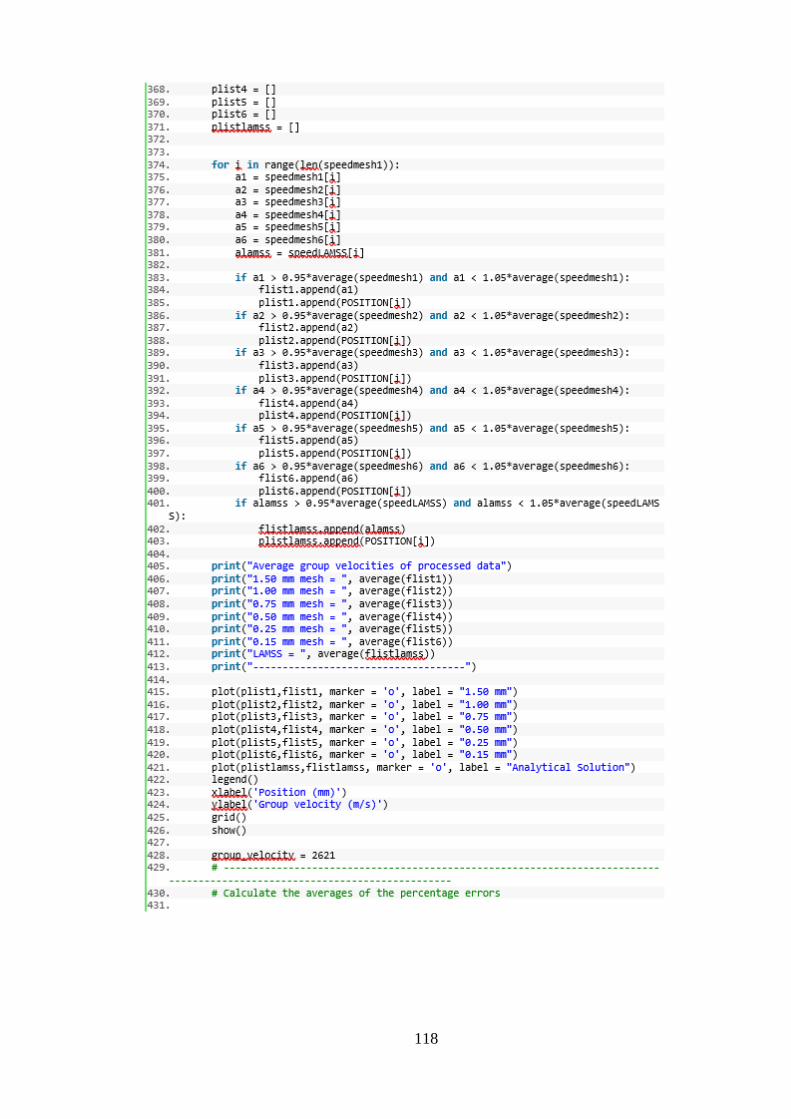
118

119

120
Appendix B: Python implementation of the 2D FFT
The Python implementation of the 2D FFT is provided in the code below.

121

122

123

124

125
Appendix C: Group velocity results for the 3D simulation
The calculated group velocities across the length of the 3D plate are presented in Figure 98
(a) along with the error relative to the theoretical value of 2621 m/s in (b). The 2D simulation
results are also presented for comparison. It can be seen that there is good overall agreement
between the two models, however the 3D FE model sees an increasing trend in error across the
plate. This resulted in a slightly higher overall numerical error for the 3D model compared with
the 2D model.
a) b)
Figure 98: The group velocity calculated across the 3D FE model shows good agreement with the 2D model (a), however
the numerical error showed an increasing trend across the length of the plate (b).
Appendix D: Reflected wave pulse group velocities
The group velocities of the A0 mode reflected from the surface notch are provided in Table
16. The group velocities were averaged to arrive at the final figure of 2583 m/s.
Table 16: Calculated group velocities of the reflected A0 mode from the surface notch.
x t1 t2 tavg cg
90 566 571 568
120 571 559 557 2542
150 555 549 543 2381
180 559 538 532 2483
210 537 525 522 2601
240 549 515 508 2542
270 526 502 498 2643
300 538 488 485 2446
330 519 479 475 2719
360 525 466 464 2612

126
390 500 464 453 2839
420 515 444 440 2626
450 494 433 429 2628
480 502 424 418 2517
Average 2583
The group velocities of the S0 mode reflected from the surface notch are provided in Table
17. The group velocities were averaged to arrive at the final figure of 5321 m/s.
Table 17: Calculated group velocities of the reflected S0 mode from the surface notch.
x t1 t2 tavg cg
90 421 442 431
120 423 427 425 4878
150 417 422 419 5106
180 411 416 414 5187
210 406 411 408 5389
240 400 405 403 5357
270 395 400 397 5422
300 389 394 392 5397
330 384 388 386 5455
360 378 383 380 5389
390 373 377 375 5414
420 367 372 369 5389
450 361 366 364 5405
480 356 361 358 5389
Average 5321
Copyright © 2022 FDOKUMEN