ARTICLE IN PRESS

Neurocomputing 71 (2008) 2727– 2741

Contents lists available at ScienceDirect

Neurocomputing

0925-23

doi:10.1

� Corr

E-m

a.hussai1 Te

journal homepage: www.elsevier.com/locate/neucom

Autonomous intelligent cruise control using a novel multiple-controllerframework incorporating fuzzy-logic-based switching and tuning

Rudwan Abdullah a,�, Amir Hussain a,1, Kevin Warwick b, Ali Zayed c

a Department of Computing Science and Mathematics, University of Stirling, Stirling, FK9 4LA, UKb Department of Cybernetics, University of Reading, Reading, RG6 6AY, UKc Seventh April University, Libya

a r t i c l e i n f o

Available online 16 May 2008

Keywords:

Intelligent adaptive control

Autonomous cruise control

Neural networks

PID control

Zero–pole placement control

Fuzzy switching

Fuzzy tuning

ETC system

12/$ - see front matter Crown Copyright & 20

016/j.neucom.2007.05.016

esponding authors. Tel.: +441786 467433; fa

ail addresses: raa@cs.stir.ac.uk (R. Abdullah),

n@cs.stir.ac.uk (A. Hussain).

l.: +441786 467437; fax: +441786 464551.

a b s t r a c t

This paper presents a novel intelligent multiple-controller framework incorporating a fuzzy-logic-based

switching and tuning supervisor along with a generalised learning model (GLM) for an autonomous

cruise control application. The proposed methodology combines the benefits of a conventional

proportional-integral-derivative (PID) controller, and a PID structure-based (simultaneous) zero and

pole placement controller. The switching decision between the two nonlinear fixed structure controllers

is made on the basis of the required performance measure using a fuzzy-logic-based supervisor,

operating at the highest level of the system. The supervisor is also employed to adaptively tune the

parameters of the multiple controllers in order to achieve the desired closed-loop system performance.

The intelligent multiple-controller framework is applied to the autonomous cruise control problem in

order to maintain a desired vehicle speed by controlling the throttle plate angle in an electronic throttle

control (ETC) system. Sample simulation results using a validated nonlinear vehicle model are used to

demonstrate the effectiveness of the multiple-controller with respect to adaptively tracking the desired

vehicle speed changes and achieving the desired speed of response, whilst penalising excessive control

action.

Crown Copyright & 2008 Published by Elsevier B.V. All rights reserved.

1. Introduction

An intelligent controller, based on an expert control concept, asa decision-making element in a feedback control loop thatrequires as much the same decision-making ability as is neededin other expert systems: however, there are significant differences.One crucial requirement is the need to provide control signals tothe process in real-time. The second requirement is that theintelligent controller should not need human interaction tocomplete its functions. The third is that the intelligent controllermust be interfaced directly to the process and be equipped withthe means for applying control to the process [5].

An intelligent controller framework based on this type of acontroller will need to combine several different control algorithmsas well as to tune the parameters of each algorithm according to thedesired user specifications. It should also automatically manage theselection between those control algorithms to maintain the controlobjectives at or near their optimal values for specific process

08 Published by Elsevier B.V. All

x: +441786 464551.

conditions. In emergency situations, where major elements in asystem break down, an intelligent controller may manage thereconfiguration of the control algorithm or switch to another moreappropriate or robust control algorithm.

Today’s automobile effectively encompasses the spirit ofmechatronic systems with its abundant applications of electro-nics, sensors, actuators, and microprocessor-based control sys-tems to provide improved performance, fuel economy, emissionlevels comfort, and safety [3,33]. For almost 2 decades, autono-mous systems have been a topic of intense research. Since themid-1980s, several research programs have been initiated all overthe world, including Advances in Vehicle Control and Safety(AVCS) in Asia, Intelligent Vehicle Highway Systems (IVHS), andPartners for Advanced Transit and Highways (PATH) in the UnitedStates. Since 2004, the US Defense Advanced Research ProjectAgency (DARPA) has started to organise the DARPA GrantChallenge to test automatic-vehicle technology [22]. In Europe,the DRIVE and PROMETHEUS projects have aimed at increasingthe safety and efficiency in normal traffic and at reducing theadverse environmental effects of the motor vehicle [8]. In France,projects such as Praxitele and ‘‘La rout automatiee’’ focus ondriving in urban environments, as do the EU’s Cybercars andCyberCars-2 projects. Another European project, Chauffeur,focuses on truck platoon driving [22]. Thus, many research

rights reserved.

ARTICLE IN PRESS

R. Abdullah et al. / Neurocomputing 71 (2008) 2727–27412728

groups are focusing on the development of functionalities forautonomous road vehicles that are able to interact with othervehicles safely and cooperatively [8,6,39].

An important component of adaptive cruise control (ACC) is todesign control systems for controlling the throttle and brake sothat the vehicle can follow the speed response of the leadingvehicle and at the same time keep a safe inter-vehicle spacingunder the constraint of comfortable driving [13,14]. Though thereare a lot of possible techniques with which to perform ACC;conventional methods based on analytical control generate goodresults but exhibit high design and computational costs since theapplication object, a car, is a nonlinear element and a completemathematical representation is impossible. As a result, othermeans of reaching human-like speed control have been recentlydeveloped, for example, through the application of artificialintelligence techniques [21].

The control of a dynamical system in the presence of largeuncertainties is of great interest at the present time. Such problemsarise when there are large parameter variations due to failures in thesystem, or due to the presence of large external disturbances [23].The application of linear control theory to these problems relies onthe key assumption of a small range of operation in order for the(local) linear model assumption to be valid. When the requiredoperating range is large, a linear controller may not be adequate. Forthis reason, it seems appropriate to use nonlinear extension ofgeneralised minimum variance-based control in order to controlcomplex plants with nonlinear models and with plant/modelmismatches. A possible way to achieve this is by incorporating theinherent nonlinearity of the process into the control design processusing a learning model [37,40,41].

The main contribution of this paper is in the development of anew intelligent multiple-controller methodology, which is appliedto an autonomous cruise control problem in order to maintain adesired vehicle speed by controlling the throttle plate angle in thecar electronic throttle control (ETC) system. The proposed frame-work employs a neural network-based generalised learning model(GLM) to minimise the effect of both the nonlinear dynamicbehaviour of the ETC system and the process disturbances. Thefuzzy-logic-based switching and tuning supervisor automaticallyselects between a proportional-integral-derivative (PID) controlleror a PID structure-based (simultaneous) pole and zero placementcontroller. Depending on the identified process phase and systembehaviour, the fuzzy-logic-based supervisor activates the appro-priate control mode. In addition, the supervisor also tunes theparameters of the multiple-controller in an on-line fashion,including the poles and zeros of the (simultaneous) pole–zeroplacement controller as well as the PID gains. All controllers aredesigned to operate using the same adaptive procedure and aselection between the various controller options is made on thebasis of the required performance measure. The supervisor canuse any available data from the control system to characterise thesystem current behaviour so that it knows which controller toactivate, the required parameters to tune, and the tuning value foreach parameter required to achieve the desired specification.

This paper is organised as follows: an overview of the controllaw and the GLM framework for the identification of nonlinearplants is presented in Section 2. The fuzzy-logic-based switchingand tuning supervisor is illustrated in Section 3, along with somereal-time implementation and stability considerations. Section 4presents the longitudinal vehicle model and the ETC systememployed for the ACC control application. Section 5 presentssimulation results to assess the effectiveness of the proposedintelligent multiple controller in tracking the desired vehiclespeed. Finally, some concluding remarks are given in Section 6.The appendix presents the closed-loop stability analysis of theproposed multiple-controller framework.

2. Description of the control law

Consider the following controlled auto-regressive movingaverage (CARMA) representation for a nonlinear plant model[37,38,40,41]

Aðz�1Þyðt þ kÞ ¼ Bðz�1ÞuðtÞ þ f 0;tðY ;UÞ þ xðt þ kÞ, (1)

where y(t) is the measured output, u(t) is the control input andx(t) is an uncorrelated sequence of random variables with zeromean at the sampling instant t ¼ 1, 2,y, and k is the time delay ofthe process in the integer-sample interval. The term f0,t(Y,U) inEq. (1) above, is potentially a nonlinear function which accountsfor any unknown time-delays, uncertainty and nonlinearity in thecomplex plant model, and can be conveniently represented by aradial basis function neural network (RBF NN) [37] multi-layeredperceptron [38,40].

The overall plant model represented by Eq. (1), is termed theGLM [37], and can be seen as the combination of a linear sub-model and a nonlinear or (learning) sub-model as shown in Fig. 1.

Also, in Eq. (1) above, y(t)AY, and u(t)AU; fY 2 Rna ;U 2 Rnb g andA(z�1) and B(z�1) are polynomials with orders na and nb,respectively, which can be expressed in terms of the backwardsshift operator, z�1 as

Aðz�1Þ ¼ 1þ a1z�1 þ � � � þ ana z�na . (2a)

Bðz�1Þ ¼ b0 þ b1z�1 þ � � � þ bnbz�nb ; b0a0. (2b)

The following control law for a multiple-controller frameworkhas been derived in [37,38] for the above nonlinear plant model

uðtÞ ¼½v ~H½Hð1Þ��1Fð1ÞwðtÞ � vFyðtÞ þ DvH0Nf 0;tð. . .Þ�

Dq0, (3)

where w(t) is the system set-point, f0,t(.,.) is a nonlinear functionrepresenting the nonlinear dynamics of the plan, v is a user-defined gain, D is the integral action required for the PID design,~H is a user-defined polynomial which can be used to introducearbitrary closed-loop zeros for an explicit pole–zero placementcontroller, H(1) is the value of ~H at the system output steady state,F is a polynomial derived from the linear parameters of thecontrolled plant and includes the desired closed-loop poles, F(1) isthe value of F at the steady state, and H0N is a user-definedpolynomial. To eliminate the effect of the nonlinear dynamics inthe steady state, H0N can be set to H0N ¼ �½Bð1Þv�

�1q0ð1Þ [37,40]. Theparameter q0 is a transfer function used to bring the closed-loopsystem parameters in the stability unit disc, and is a polynomial inz�1 having the following form: q0ðz�1Þ ¼ 1þ q01z�1 þ q02z�2 þ � � �þ

q0nq0z�nq0 , where nq0 is the degree of the polynomial q0.

It can be seen from the control law in Eq. (3) above that thecontroller denominator is split into two parts, namely: anintegrator action part (D) required for PID design; and an arbitrarycompensator (q0) that may be used for simultaneous pole and zeroplacement designs. Moreover, the polynomials H0N and q0 can beused to switch on and off the two controlling modes of themultiple controller, both of which are presented next.

2.1. Multiple-controller mode 1: PID controller

In this mode, the multiple controller operates as a conventionalself-tuning PID controller, which can be expressed in the mostcommonly used velocity form [34] as

DuðtÞ ¼ KIwðtÞ � ½KP þ KI þ KD�yðtÞ

� ½�KP � 2KD�yðt � 1Þ � KDyðt � 2Þ. (4)

ARTICLE IN PRESS

y(t)

-

Plantu (t)

PID pole-zero Placement controller

Fuzzy Logic Based Switchingand Tuning Supervisor

Switch

Controller Design: 1) Compute F and

q′2) Set:

~~H = F(1)H[H(1)]−1.

f0, t (.,.)

−y(t)

f0, t (.,.)

+

w(t) Set-point +

Behaviour Recogniser

-

Switching signal

Tuning signal

GLM

RBF-NN Nonlinear Sub-model

RLS Linear sub-model

+

Switching Logic

Tuning Logic

w(t)Set-point

H

User inputs

PID controller

� (t)

� (t)

Fig. 1. Nonlinear multiple controller incorporating the GLM and fuzzy supervisory switching and tuning.

R. Abdullah et al. / Neurocomputing 71 (2008) 2727–2741 2729

To obtain a self-tuning PID controller, the degree of F(z�1) is set to 2so that

Fðz�1Þ ¼ f 0 þ f 1z�1 þ f 2z�2 (5)

and both the pole-placement polynomial q0 and zero placementpolynomial ~H are switched off by setting

q0ðz�1Þ ¼ 1; ði:e: q01 ¼ q02 ¼ � � � ¼ q0nq0¼ 0Þ;

~H ¼ 1; ði:e: ~h1 ¼~h2 ¼ � � � ¼

~hn ~h¼ 0Þ:

9=;. (6)

Therefore, the self-tuning PID controller is structured as follows:

DuðtÞ ¼ ½vFð1ÞwðtÞ � vðf 0 þ f 1z�1 þ f 2z�2ÞyðtÞ

þ DvH0Nf 0;tð:; :Þ�, (7)

Kp ¼ �v½f 1 þ 2vf 2�, (8)

KI ¼ v½f 0 þ f 1 þ f 2�, (9)

KD ¼ vf 2. (10)

It can be seen from the above Eqs. (7)–(10) that the PID controlparameters Kp, KI and KD depend on the polynomial matrix F(z�1)and the gain v [34].

The main disadvantage of PID self-tuning-based minimumvariance control designs, in general, is that the tuning parametersmust be selected using a trial and error procedure. That said, theuse of general heuristics can provide reasonable closed-loopperformance. Alternatively, the tuning parameters can also beautomatically and implicitly set on-line by specifying the desiredclosed-loop poles [17,32].

2.2. Multiple-controller mode 2: simultaneous zero and

pole placement controller based on a PID structure

To derive a simultaneous zero and pole-placement controllerwith a PID structure, the transfer function of the closed-loopsystem must be derived. Substituting for u(t) given by Eq. (3) intothe process model described by Eq. (1), the closed-loop system is

obtained as follows:

ð ~Aq0 þ z�1 ~BFÞyðtÞ ¼ z�1Bv ~H½Hð1Þ��1Fð1ÞwðtÞ

þ DðZ�1BvH0N þ q0Þf 0;t þ Dq0, (11)

where ~A ¼ DA and ~B ¼ vB.The following Diophantine equation is used to place poles of

the system in the required position [37]

ðq0 ~Aþ z�1F ~BÞ ¼ T , (12)

where T represents the desired closed-loop poles and q0 is thecontroller polynomial. For Eq. (12) to have a unique solution, theorder of the regulator polynomials and the number of the desiredclosed-loop poles can be set as [4,24,32]

nf 0 ¼ n ~a � 1 ¼ na

nq0 ¼ n ~b þ k� 1

ntpn ~a þ n ~b þ k� 1

9>=>;, (13)

where n ~a, n ~b and nq0 are the orders of the polynomials ~A, ~B and q0,respectively, and nt denotes the number of desired closed-looppoles. Also, n ~b ¼ nb and n~a ¼ na þ 1.

Combining Eqs. (11) and (12) and setting

H0N ¼ �½Bð1Þv��1q0ð1Þ, (14)

Tðz�1Þ ¼ 1þ t1z�1 þ t2z�2 þ � � � þ tnt z�nt , (15)

~Hðz�1Þ ¼ 1þ h1z�1 þ h2z�2 þ � � � þ h ~hz�~h, (16)

where nh and nt represent orders of the polynomials H(z�1) andT(z�1), respectively. An arbitrary desired zeros polynomial can beused to reduce excessive control action, which can result from set-point changes when pole placement is used.

The final closed-loop function for the zero and pole-placementcontroller then becomes

TyðtÞ ¼ z�1Bv½ ~Hð1Þ��1 ~HFð1ÞwðtÞ þ Dðz�1Bvq0ð1Þ

�½�ðBð1ÞvÞ�1� þ q0Þf 0;t þ Dq0xðtÞ. (17)

ARTICLE IN PRESS

R. Abdullah et al. / Neurocomputing 71 (2008) 2727–27412730

Note that, in practice, the order of T(z�1) and H(z�1) are most ofthe time selected to equal 1 or 2 [34]. It can be seen from Eq. (17)that the closed-loop poles and zero are placed at their desiredpositions which are pre-specified by using the polynomials T(z�1)and H(z�1).

In the next section, the identification of complex nonlinearplants using the GLM framework is briefly discussed.

2.3. GLM for the identification of nonlinear plants

A wide range of nonlinear dynamic plants can be described bya discrete time equation [41] y(t+1) ¼ f(Y,U) where f(Y,U)-Rn;fY 2 Rny ;U 2 Rnu ;n ¼ ny þ nug is a complicated nonlinear function,and y(t)AY and u(t)AU are the plant output and input signals,respectively, at discrete times tA1, 2,y . To control such anonlinear plant, the generalised parametric time-varying plantmodel described in Eq. (1) is considered [37,38,40,41]. In addition,it is assumed that the parameters associated with A(z�1) andB(z�1) (in Eq. (1)) are either time invariant or slowly time varying.On the other hand, f(Y,U)-Rn is potentially a time-varyingnonlinear function. Therefore, the equivalent plant model is acombination of a linear time-varying sub-model plus a nonlineartime-varying sub-model (or an error agent), which have beencollectively termed the GLM [37]. The linear sub-model is used toapproximate the dominant linear dynamics of the nonlineardynamic plant around its operating point. On the other hand, the‘learning’ error agent is used to learn the errors from the linearsub-model that are due to nonlinearities, uncertainties, distur-bances and model mismatch in the controlled plant.

The GLM model is illustrated in Fig. 1, where a recursive least-squares algorithm is initially used to estimate the parameters A

and B (Eq. (1)) of the linear sub-model, and an RBF NN-basedlearning model is subsequently used to approximate the nonlinearpart f0,t(.,.).

It can be seen from Eq. (1) that the measured output y(t) can beobtained as follows [40]:

yðt þ 1Þ ¼ jT ðtÞyþ f 0;tðy;uÞ, (18)

y ¼ ½�a1; . . . ;�ana ; b0; . . . ; bnb�

jT ¼ ½yðt � 1Þ; . . . ; yðt � naÞ;uðt � 1Þ; . . . ;uðt � nbÞ�

). (19)

From Fig. 1 we can also see that f0,t(.,.) can be expressed as

f 0;tð:; :Þ ¼ f 0;tð:; :Þ þ �ðtÞ. (20)

Using the above Eq. (20), and as shown in Fig. 1, an NN can beeffectively used for estimating the nonlinear error function f0,t,with the identification error e(t) used to update the weights andthresholds of the learning neural network model. The neuralnetwork model employed in the proposed control scheme here ischosen to be the linear-in-parameters RBF NN as opposed to thecomputationally more expensive multi-layer perceptron (MLP)previously used in [40]. The RBF NNs can improve the systemdamping and dynamic transient stability more effectively than theMLP NNs [26]. In addition, the RBF requires a lower computationalcomplexity and elapsed time to train the network on-line,compared to the MLP [26]. The RBF NNs ability to uniformlyapproximate smooth functions over compact sets is well docu-mented in the literature, see for example [30].

Using the RBF NN, the nonlinear function f0(.,.) is adaptivelyestimated by using the following equations [37]:

f 0;tð:; :Þ ¼Xn

j¼1

wjgjb, (21)

dw ¼ Zgj;tf 0;t ½f 0;t � f 0;t�½1� f 0;t�, (22)

wjðtÞ ¼ wjðt � 1Þ þ dw, (23)

g0;tð. . .Þ ¼ exp �Xl

i¼1

kxi � cijk

2

ð2sijÞ

2

!, (24)

where wj represents the hidden layer weights, b is the outputlayer threshold, dw is the change in weights, Z is the learning rate,xi is the inputs, cj

i is the centre of Gaussian basis function of the jthhidden unit, l ¼ na+nb, and gj is the output of the hidden layer. Thevariance of the Gaussian units sj

i is dependent on the inputdimension because the RBF inputs are scaled differently [18,27].RBF weights can be adapted using various algorithms, as goodoverview of which can be found in [10].

2.4. Discussion on selection of controller type and switching issues

Due to the robustness, simplicity of structure, ease ofimplementation, and remarkable effectiveness in regulating awide range of processes, the conventional self-tuning PIDcontroller (multiple-controller mode 1) proposed in Section 2.1should normally be the first choice to obtain satisfactory closed-loop system performance. If, however, a better closed-loopperformance based on, say, a desired damping ratio, rise time,settling time overshoot, system bandwidth or the actual mini-mum variance performance index-is required, or if the complexsystem to be controlled is difficult to tune using a conventionalself-tuning PID controller—due to, for example, an excessivecontrol (input) action resulting from set-point changes, addeddisturbances and/or plant nonlinearity—then the PID structure-based (simultaneous) pole and zero placement controller (multi-ple-controller mode 2) discussed in Section 2.2 can be used as asecond choice. However, this will be at the expense of a greatercomputational effort required for implementation of the (simul-taneous) pole and zero placement controller [37,38]. Note thatwhilst only two control modes have been considered here, theproposed framework is flexible enough to allow additionalcontrollers to be employed in order to further improve theclosed-loop performance, if required. In the context of switchingbetween the above two controller modes, the type of discriminat-ing (system performance) criteria mentioned above can also beused to design an intelligent fuzzy-logic-based switching andtuning supervisor, which is presented in the next section.

3. Fuzzy-logic-based switching and tuning supervisor

The fuzzy-logic-based switching and tuning supervisor issituated at the highest level of the multiple-controller framework.Following [28], the fuzzy supervisor can use any available datafrom the control system to characterise the system currentbehaviour so that it knows which controller to choose, whichparameters to tune, and the tuning value for each parameter thatis required to ultimately achieve the desired specification. Themain idea behind the fuzzy-logic supervisor approach here is toemploy logic-based switching and tuning among the family of thecandidate controllers. The need for switching stems from the factthat typically no single controller can guarantee the desiredbehaviour when connected with a poorly modelled process, andparticularly so for the case of complex processes exhibitingsignificant nonlinearity, nonstationarity, uncertainty and/ormulti-variable interactions [37]. Such switching schemes canprovide an alternative to more traditional continuously tunedadaptive control algorithms.

Following [1,11,28], the supervisor employed in this workcomprises two sub-systems: a behaviour recogniser and a switching

and tuning logic (see Fig. 1). The supervisor aims to recognise when

ARTICLE IN PRESS

0.2

0

0.4

0.6

0.8

1Decreasing IncreasingNorm

0-1

0.2

0

0.4

0.6

0.8

1

0

PID

5

Pole Zero Place

40

0.2

0

0.4

0.6

0.8

1

60 1000 908010 7020 30 50

HighNorm

0.2

0

0.4

0.6

0.8

1 Norm High

-100 -80

- High

100

Deg

ree

of M

embe

rshi

p D

egre

e of

Mem

bers

hip

Deg

ree

of M

embe

rshi

pD

egre

e of

Mem

bers

hip

-60 -40 -20 20 40 60 800 40

1 10 15 20 25 30 35

Fig. 2. (a) Membership function of the overshooting input parameter, (b) membership function of the input signal variance input parameter, (c) membership functions of

reference signal changes input parameter and (d) membership function of the controller selection output parameter.

R. Abdullah et al. / Neurocomputing 71 (2008) 2727–2741 2731

the system requires selection of another controller, or when aselected controller is not properly tuned, and then seeks to switchto the candidate controller and/or adjust the controller para-meters to obtain improved performance. The whole supervisor isimplemented using simple fuzzy-logic-based switching andtuning rules where the premises of the rules form part of thebehaviour recogniser and the consequent form the switching andtuning decision. In this way, a simple fuzzy system is used toimplement the entire supervisory control level.

3.1. Behaviour recogniser

The behaviour recogniser seeks to characterize the currentbehaviour of the plant in a way that will be useful to the switchingand tuning logic sub-systems [29]. The behaviour of the system ischaracterized through the on-line estimation of five parametersnamely: the overshoot of the closed-loop system output signal, thevariance of the control input signal, rise and fall times of theoutput signal (used for tuning purposes), reference signal (i.e. set-point) changes, and the system steady-state error. In order toprevent the so-called shattering problem (Zeno behaviour) causedby wrongly designed switching rules [11], which can result in aninfinite number of switchings between controller modules, theaverage of the current and last two values of the overshootmeasurements are used as an output parameter from thebehaviour recogniser. The output signal rise and fall timesrepresent the amount of time for a signal to change state. Tomeasure rise and fall times, the behaviour recogniser tracks 10%and 90% values of the output signal. The PID controller steady-state error is used to tune the gain v (Eq. (3)).

3.2. Switching logic

The key task of the switching logic sub-system is to generate aswitching signal which determines, at each instant of time, thecandidate controller module that is to be activated [1,11]. Theswitching logic is implemented using fuzzy-logic rules where

the premises of the rules use the output of the behaviourrecogniser as input parameters, and the consequents of rulesform the controller selection decision (output parameter).Fig. 2a–c, respectively, shows the shape of the membershipfunctions of the system output overshoot, control input-varianceand reference signal changes, which are all input parameters forthe switching decision. Fig. 2d shows the membership function ofthe controller selection output parameter. The complete rule setfor the fuzzy supervisor switching logic is given below:

If Overshoot is High OR Control input-variance is High Then

Controller is Pole-Zero PlacementIf Overshoot is High OR Control input-variance is High Then

Controller is Pole-Zero PlacementIf Reference signal is Not Norm Then Controller is Pole-ZeroPlacementIf Overshoot is Norm OR Control input-variance is Norm Then

Controller is PID

Depending on the fuzzified value of the two input parameters,the switching logic sub-system will switch either to the conven-tional PID controller, or PID structure-based (simultaneous) poleand zero placement controller. The middle-of-max approach isused for de-fuzzification in order to identify the selectedcontroller.

3.3. Tuning logic

The key task of the tuning logic sub-system is to tune theparameters of the multiple-controller on-line, including poles andzeros of the (simultaneous) pole-zero placement controller inaddition to the PID gains. The tuning facility aims to make thesystem achieve a desired speed of response and/or minimize thecontrol input action. Using the measurements of the rise time andfall time of the output signal, which are measured by thebehaviour recogniser sub-system, and detected changes inthe reference signal, the fuzzy-logic-based supervisor will specify

ARTICLE IN PRESS

0.2

0

0.4

0.6

0.8

1average slower faster

-0.8

0.2

0

0.4

0.6

0.8

1

0 10 …162 144 6 8

slowfast norm

Deg

ree

of M

embe

rshi

p

Deg

ree

of M

embe

rshi

p0.2

0

0.4

0.6

0.8

1decrease increase

0.2

0

0.4

0.6

0.8

1Decreasing Increasing Norm

0-1

0.2

0

0.4

0.6

0.8

1decrease increase

0.2

0

0.4

0.6

0.8

1

-10

high -high norm

Deg

ree

of M

embe

rshi

pD

egre

e of

Mem

bers

hip

Deg

ree

of M

embe

rshi

pD

egre

e of

Mem

bers

hip

12 100 -0.6 -0.4 -0.2 0.20 0.4 0.6 0.8

-0.8

-8 -6 -4 0 2 4 6 8

-0.6 -0.4 -0.2 0.20 0.4 0.6 0.81

-0 10

Fig. 3. (a) Membership function of the rise time parameter, (b) membership function for poles tuning output parameter, (c) membership functions of set-point changes input

parameter, (d) membership functions zeros tuning parameter, (e) membership function of the PID steady-state error parameter and (f) membership function for PID gain

tuning output parameter.

R. Abdullah et al. / Neurocomputing 71 (2008) 2727–27412732

the tuning values for the active/selected controller’s parameters.The complete fuzzy rule set for parameter tuning is given below:

IF Rising-time is norm AND controller is Pole-Zero PlacementTHEN poles-tuning is no-changeIF Rising-time is fast AND controller is Pole-Zero PlacementTHEN poles-tuning is slowerIF Rising-time is slow AND controller is Pole-Zero PlacementTHEN poles-tuning is fasterIF set-point is increasing AND controller is Pole-Zero PlacementTHEN zeros-tuning is decreaseIF set-point is decreasing AND controller is Pole-Zero PlacementTHEN zeros-tuning is increaseIF Control input-variance is high AND controller is PID THEN gain

is decreaseIF steady-state-error is high AND controller is PID THEN gain isdecreaseIF steady-state-error is high AND controller is PID THEN gain isincreaseIF steady-state-error is norm AND controller is PID THEN gain isno-change

The fuzzy membership functions used for tuning the controllerparameters are shown in Fig. 3a–f.

3.4. Real-time implementation and stability considerations

Two key real-time implementation constraints include mini-mising the amount of memory used and the time taken tocompute the fuzzy outputs from given inputs [28]. Keeping thesein view, the proposed fuzzy-logic-based switching and tuningsupervisor has been designed with a minimum number of fuzzyrules along with minimum input and output parameters. Theswitching logic consists of a total of six rules, two inputparameters and one output parameter. The tuning logic comprisesnine rules, three inputs and three output parameters. From thepoint of view of computational complexity, a maximum of threemembership functions are considered for both the inputs andoutputs with no more than two overlapping membershipfunctions. In order to improve the computation time, thetriangular and trapezoidal membership functions are used, whichhave the advantages of simplicity and require minimum rules. Toreduce the memory requirements and to enable online operation

ARTICLE IN PRESS

R. Abdullah et al. / Neurocomputing 71 (2008) 2727–2741 2733

(i.e., switching and tuning), the fuzzy supervisor is designed tocompute the rule-base at each time instant rather than using astored one. Future implementation prospects can be improved byusing a state-of-the-art microprocessor or signal processing chip.An alternative would be to investigate the advantages anddisadvantages of using a fuzzy processor (i.e., a processordesigned specifically for implementing fuzzy controllers) asin [28].

Finally, note that a theoretical verification of the stability of theproposed multiple-controller framework is important especiallyfor safety-critical systems such as the target ACC applicationconsidered in this work. The closed-loop stability analysis of theproposed controller framework is summarised in Appendix A.

4. Description of the application model employed

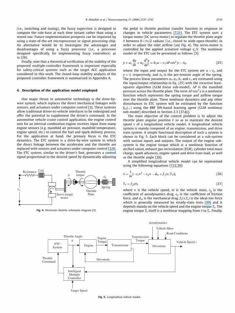
One major thrust in automotive technology is the drive-by-wire system, which replaces the direct mechanical linkages withsensors, and actuators under computer control [3]. These systemsallow traditional driver-to-vehicle interfaces to be redesigned andoffer the potential to supplement the driver’s command. In theautomotive vehicle cruise control application, the engine controlunit for an internal combustion engine receives input from manyengine sensors (e.g. manifold air pressure, manifold temperature,engine speed, etc.) to control the fuel and spark delivery process.For the application at hand, the primary focus is the ETCdynamics. The ETC system is a drive-by-wire system in whichthe direct linkage between the accelerator and the throttle arereplaced with sensors and actuators under computer control [3,9].The ETC system, similar to the driver’s foot, generates a controlsignal proportional to the desired speed by dynamically adjusting

ea

Resistance Coil

ThrottlePlate

Spring

Servo torquemotor

Throttletorque

�0�

Fig. 4. Electronic throttle schematic diagram [3].

Engine

ThrottleCommand

Engine Torque

Drivetrain

Transmis

Target Speed

ETCSystem

IntelligentMultiple

Controller

Throttle Angle

�

Fig. 5. Longitudinal

the pedal to throttle position transfer function in response tochanges in vehicle parameters [7,21]. The ETC system uses atorque motor (DC servo-motor) to regulate the throttle plate angley between 0oyp/2 radians (i.e., closed to wide-open-throttle) inorder to adjust the inlet airflow (see Fig. 4). The servo-motor iscontrolled by the applied armature voltage ea V. The nonlinearmodel of the ETC can be presented as follows [3]:

yþ a1dy

dtþ a2

d2y

dt2¼ b1u� c1DP cos2 y� y0, (25)

where the input and output for the ETC system are u ¼ ea andy ¼ y, respectively, and y0 is the pre-tension angle of the spring.The process linear parameters a1, a2, b1 and c1 are estimated usingthe input/output relationship in Eq. (25) with the recursive least-squares algorithm (GLM linear sub-model). DP is the manifoldpressure across the throttle plate. The term DP cos2 y is a nonlinearfunction which represents the spring torque and airflow torqueover the throttle plate. These nonlinear dynamics and any otherdisturbances in ETC system will be estimated by the functionf0,t(.,.) using the RBF NN-based learning agent (GLM nonlinearsub-model) described in Section 2.3 [37,41].

The main objective of the control problem is to adjust thethrottle plate angular position y so as to maintain the desiredspeed v of a longitudinal vehicle model. A longitudinal vehiclesystem is mainly composed of an engine, transmission, and drivetrain system. A simple functional description of such a system isshown in Fig. 5. Each block can be considered as a sub-systemwith various inputs and outputs. The output of the engine sub-system is the engine torque which is a nonlinear function ofair/fuel ration, exhaust gas recirculation (EGR), cylinder total masscharge, spark advances, engine speed and drive train load, as wellas the throttle angle [39].

A simplified longitudinal vehicle model can be representedusing the following equations [7,12,39]:

_v ¼1

m½�cvv2 � cpv� dm þ f 1ðv; TeÞ�, (26)

Te ¼ f 2ðyÞ, (27)

where v is the vehicle speed, m is the vehicle mass, cv is thecoefficient of aerodynamics drag, cp is the coefficient of frictionforce, and dm is the mechanical drag. f1(v,Te) is the ideal-tire forcewhich is generally measured by steady-state tests [39] and itdepends mainly on the vehicle speed and the engine torque Te. Theengine torque Te itself is a nonlinear mapping from y to Te. Finally,

Vehicle Speed vDrivetrain

TransmissionTorque

Aerodynamics

Vehicle Mass

Road Conditions

sion

vehicle model.

ARTICLE IN PRESS

R. Abdullah et al. / Neurocomputing 71 (2008) 2727–27412734

f2(y) is the steady-state characteristics of engine and transmissionsystems, and in this paper it is represented by an RBF NN with y asits input, and Te as the output variable. The RBF design parameterswere selected on a trial and error basis.

Note that as discussed in [39], the above vehicle dynamicsequations (26) and (27) have the following property: for any givendesired ideal-tire force and velocity v, there exists a uniquethrottle angle input y that achieves the desired ideal-tire force.Further details on the above model can be found in [39].

5. Simulation results

In order to assess the performance of the proposed schemein controlling the ETC system for an autonomous cruise controlapplication, 3 experiments are performed and presented inthis section. All simulation examples are performed over 1000samples to track a reference signal representing the target vehiclespeed changes. The desired closed-loop pole and zero polynomialsare initially selected as T ¼ 1�0.4z�1

�0.2z�2 and h ¼ 1+0.9z�1+0.6z�2. In order to achieve the PI self-tuning case for thisapplication, the user-defined parameters are selected as: P ¼ 1and v ¼ 0.83. The nonlinear function f0,t(.,.) representing thenonlinear dynamics of the ETC system is obtained usingEqs. (21)–(24), which implement the nonlinear sub-model of thecomplex ETC system. Using a trial- and -error approach, the RBFNN was designed with eight units in the hidden layer three ofwhich had fixed centres and the remaining five units wereselected to have adaptive centres and were fine tuned using theback-propagation method (as in) [25]. The output layer weightswere updated using the Delta rule.

The problem of regulating the throttle plate in the ETC systemcan be divided into three sub-problems: firstly, preventing over-shooting in control of the throttle plate angle caused by eitherreference signal changes, nonlinear system dynamics and/or addeddisturbances; secondly, minimising any high-voltage inputs appliedto the DC servo-motor in the ETC system; and finally, minimisingoscillation in the normal system (steady state) operation.The controller that solves best the first and second sub-problemsis the PI structure-based pole–zero placement controller (at theexpense of a relatively greater computational requirement),whereas the controller that most effectively deals with the thirdsub-problem is the conventional PI controller. The fuzzy-logic-based switching and tuning supervisor is designed to automaticallyswitch between these two controllers on the basis of the systembehaviour detected by the behaviour recogniser sub-system. Thetuning logic is used to regulate each controller’s parameters inorder to achieve the desired (user specified) signal rise and falltimes, and to reduce the magnitude of the control input signalintroduced to the throttle actuator (i.e., the DC servo-motor). In thefollowing 2 experiments, the ETC system is controlled using each ofthe two individual multiple-controller modes (with no switching).In the final third experiment, the intelligent multiple-controller isdeployed incorporating fuzzy-logic-based switching between thetwo controller modes. The aim is to justify the need for, anddemonstrate the advantages of deploying the proposed intelligentmultiple-controller framework incorporating a fuzzy-logic-basedswitching and tuning supervisor. In all experiments, the nonlinearsub-model of the GLM was set to work with the linear sub-modelin order to incorporate f0,t(.,.) in the control law.

5.1. Experiment 1

In this experiment, the multiple-controller was set to controlthe ETC system using only the conventional PI controller(multiple-controller mode 1).

In the obtained results, Fig. 6a–d, respectively, shows thevehicle speed signal obtained (when the PI controller is used tomaintain the target vehicle speed v), the output throttle plateangle y (required to reach the target speed), the throttle controlinput signal u(t) applied to the torque motor (to produce therequired throttle angle y), and the system nonlinearities andexternal disturbances applied to the controlled ETC system.

Fig. 6b and c shows high overshooting in both the outputthrottle angle signal and in the throttle control input signal,respectively, when the reference signal changes. The use of thePI only controller resulted in this overshooting as it worked toproduce the required output throttle angle to track the targetchanges in speed. On the other hand, as can be seen from Fig. 6b,as expected theoretically, the PI controller has the advantage ofmaintaining relatively smooth steady performance. In addition,Fig. 6b and c also shows relatively low overshooting at samplingtime 300 caused by the presence of nonlinear dynamics of theETC system, and the externally introduced constant and randomdisturbances. The variance of the control input signal wasmeasured to equal 0.0030, and the variance of the output (throttleangle) signal was 0.0305.

5.2. Experiment 2

In this experiment, the multiple-controller was set to controlthe ETC system using only the pole–zero placement controller(multiple-controller mode 2).

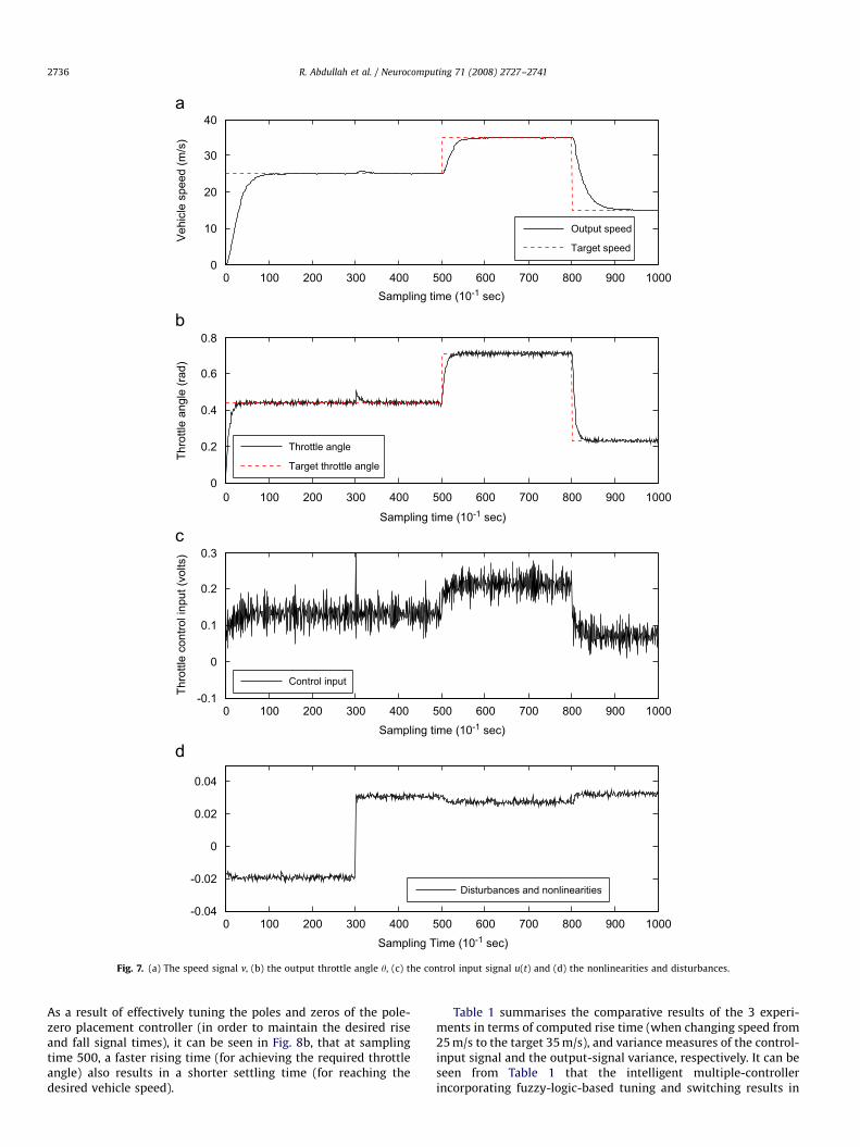
In the obtained results, Fig. 7a–d, respectively, shows thevehicle speed signal obtained, the output throttle plate angle y,the throttle control input signal u(t) and the system nonlinearitiesand external disturbances applied to the controlled ETC system.

In the obtained results, Fig. 7b and c shows relatively higherovershooting at sampling time 300 caused by the presence ofnonlinear dynamics of the ETC system, and the externallyintroduced constant and random disturbances. In addition,continuous sharp oscillations can be seen during the steady statewhile the pole–zero placement controller worked to produce therequired output throttle angle for effectively tracking the desiredspeed changes. However, as expected theoretically, this pole–zeroplacement controller exhibits very low overshooting while dealingwith reference signal changes (as can be seen from Fig. 7b) as aresult of effectively minimising the control input-variance (shownin Fig. 7c). The variance of the control input signal was measuredto equal 0.0027 and the variance of the throttle angle signal was0.0278.

5.3. Experiment 3

In this example, the intelligent multiple controller was set toautomatically control the ETC system in order to track the definedvehicle speed reference signal. By appropriately switchingbetween the conventional nonlinear PI controller and the non-linear pole–zero placement controller (based on the monitoreddegree of overshooting and input signal variance), the fuzzy-logic-based supervisor works to prevent any overshooting andminimises the steady-state oscillations while controlling theETC system. The capability of the fuzzy-logic-based supervisorto tune the controller parameters also allows for controlling therise and fall times of the output signal (throttle angle) accordingto user-defined requirements.

In the obtained results, Fig. 8a–e, respectively, shows thevehicle speed signal obtained, the output throttle plate angle y,the throttle control input signal u(t), the selection schemeresulting from use of the fuzzy-logic-based switching supervisor,

ARTICLE IN PRESS

0 100 200 300 400 500 600 700 800 900 10000

10

20

30

40

Sampling time (10-1 sec)

Veh

icle

spe

ed (m

/s)

Output speedTarget speed

0 100 200 300 400 500 600 700 800 900 10000

0.2

0.4

0.6

0.8

Sampling time (10-1 sec)

Thro

ttle

angl

e (r

ad)

Throttle angleTarget throttle angle

0 100 200 300 400 500 600 700 800 900 1000-0.1

0

0.1

0.2

0.3

Sampling time (10-1 sec)

Thro

ttle

cont

rol i

nput

(vol

ts)

Control input

0 100 200 300 400 500 600 700 800 900 1000-0.04

-0.02

0

0.02

0.04

Sampling Time (10-1 sec)

Disturbances and nonlinearities

Fig. 6. (a) The speed signal v, (b) the output throttle angle y, (c) the control input signal u(t) and (d) the nonlinearities and disturbances.

R. Abdullah et al. / Neurocomputing 71 (2008) 2727–2741 2735

and system nonlinearities and external disturbances applied tothe controlled ETC system.

Compared to the results obtained from experiments 1 and 2, itcan be seen from Fig. 8(a)–(d) that the fuzzy-logic-based super-visor effectively manages to prevent output signal (throttle angle)

overshooting and simultaneously preserves relatively smoothsteady-state input and output signals. Another point to note isthat the excessive control action (resulting from reference set-point changes) is tuned most effectively when the switchingsupervisor activates the PI-based pole–zero placement controller.

ARTICLE IN PRESS

0 100 200 300 400 500 600 700 800 900 10000

10

20

30

40

Sampling time (10-1 sec)

Veh

icle

spe

ed (m

/s)

Output speed

Target speed

0 100 200 300 400 500 600 700 800 900 10000

0.2

0.4

0.6

0.8

Sampling time (10-1 sec)

Thro

ttle

angl

e (r

ad)

Throttle angle

Target throttle angle

0 100 200 300 400 500 600 700 800 900 1000-0.1

0

0.1

0.2

0.3

Sampling time (10-1 sec)

Thro

ttle

cont

rol i

nput

(vol

ts)

Control input

0 100 200 300 400 500 600 700 800 900 1000-0.04

-0.02

0

0.02

0.04

Sampling Time (10-1 sec)

Disturbances and nonlinearities

Fig. 7. (a) The speed signal v, (b) the output throttle angle y, (c) the control input signal u(t) and (d) the nonlinearities and disturbances.

R. Abdullah et al. / Neurocomputing 71 (2008) 2727–27412736

As a result of effectively tuning the poles and zeros of the pole-zero placement controller (in order to maintain the desired riseand fall signal times), it can be seen in Fig. 8b, that at samplingtime 500, a faster rising time (for achieving the required throttleangle) also results in a shorter settling time (for reaching thedesired vehicle speed).

Table 1 summarises the comparative results of the 3 experi-ments in terms of computed rise time (when changing speed from25 m/s to the target 35 m/s), and variance measures of the control-input signal and the output-signal variance, respectively. It can beseen from Table 1 that the intelligent multiple-controllerincorporating fuzzy-logic-based tuning and switching results in

ARTICLE IN PRESS

0 100 200 300 400 500 600 700 800 900 10000

10

20

30

40

Sampling time (10-1 sec)

Veh

icle

spe

ed (m

/s)

Output speed

Target speed

0 100 200 300 400 500 600 700 800 900 10000

0.2

0.4

0.6

0.8

Sampling time (10-1 sec)

Thro

ttle

angl

e (r

ad)

Throttle angle

Target throttle angle

0 100 200 300 400 500 600 700 800 900 1000-0.1

0

0.1

0.2

0.3

Sampling time (10-1 sec)

Thro

ttle

cont

rol i

nput

(vol

ts)

Control input

0 100 200 300 400 500 600 700 800 900 1000Inactive

Active

Inactive

Active

Sampling time (10-1 sec)

0 100 200 300 400 500 600 700 800 900 1000-0.04

-0.02

0

0.02

0.04

Disturbances and nonlinearities

pole-Zero placement controller

PID controller

Sampling Time (10-1 sec)

Fig. 8. (a) The speed signal v, (b) the output throttle angle y, (c) the control input signal u(t), (d) the switching scheme and (e) the nonlinearity and disturbances.

R. Abdullah et al. / Neurocomputing 71 (2008) 2727–2741 2737

ARTICLE IN PRESS

Table 1Summary of comparative minimum variance performance

(Control) input signal

variance

(Throttle angle) output

signal variance

Rise time to target speed

(35 m/s) (s)

Experiment 1 (PI controller mode only) 0.0030 0.0305 6.3

Experiment 2 (Pole–zero placement controller mode only) 0.0027 0.0278 8.7

Experiment 3 (multiple-controller with intelligent switching

between PI and pole–zero placement controllers)

0.0028 0.0300 4.2

R. Abdullah et al. / Neurocomputing 71 (2008) 2727–27412738

improved performance (both in terms of minimum output-signalvariance and rise-times) compared to the stand-alone PI only andpole–zero placement only controllers. These preliminary resultsdemonstrate the need for, and advantages of effectively switchingbetween, and tuning the two multiple controllers using a fuzzy-logic-based supervisor.

Note that another switching issue, which has not beenaddressed theoretically in this work relates to a potential problemassociated with conventional multiple-controller switching para-digms of having to achieve a smooth bumpless transfer whenswitching between controllers [1]. It is always desirable toperform bumpless switching between different controlling sce-narios, i.e., switching that does not induce a large transientbecause of incompatible ‘‘initial conditions’’ of the controllerconnected to the plant and of the plant itself [36]. On the otherhand, as is evident from the sample simulation results above,our proposed framework appears to exhibit the desired bump-less switching between the two controllers. An intuitive explana-tion of this is that the two multiple-controller modes are derivedfrom a single minimum variance-based cost function, whichguarantees compatible initial conditions for both controllers.As a result, the switching decision is made in an integral mannerby modifying the common control law (contrary to thecase with other classical multiple-controller-switching frame-works) [37].

6. Conclusions

In this paper, a new intelligent nonlinear multiple-controllerframework incorporating a fuzzy-logic-based switching andtuning supervisor is developed. The framework integrates thesimple fuzzy-rule-based supervisor with the benefits of both theconventional PID and PID-structured pole–zero placement non-linear controllers along with a GLM framework. In the GLM, theunknown complex process to be controlled is represented by anequivalent stochastic model consisting of a linear time-varyingsub-model plus a computationally efficient RBF NN-based learn-ing sub-model. The proposed methodology provides the designerthe choice between the conventional PID self-tuning controller, orthe PID structure-based (simultaneous) pole and zero placementcontroller. Both controllers (multiple-controller modes) benefitfrom the simplicity of having a PID structure, operate using thesame adaptive procedure and can be selected on the basis of therequired performance measure. The switching decision betweenthe two nonlinear fixed structure controllers, along with on-linetuning of the controller parameters, is made using a fuzzy-logic-based supervisor operating at the highest level of the system. Theproposed intelligent framework is applied to the nonlinearETC system for an autonomous cruise control application. Samplesimulation results using a validated nonlinear vehicle model areused to demonstrate the effectiveness of the multiple-controllerwith respect to adaptively tracking desired vehicle speed changesand achieving the desired speed of response, whilst penalisingexcessive control action.

For future work, the proposed controller framework will beimplemented on a test-bed vehicle in real-time in order to furtherassess its ability to adapt the vehicle speed to a pre-defined leveland additionally, to maintain a safe headway distance (gap)between the controlled vehicle and a preceding vehicle. Also, notethat whilst only two controller modes have been considered inthis paper, the proposed intelligent switching and tuning super-visory framework readily allows additional controllers to beemployed in order to further improve the closed-loop perfor-mance. This will also be investigated in future work.

Appendix A. Closed-loop stability analysis of themultiple-controller framework

Stability of the proposed control algorithm for the ACCproblem is analysed based on the following assumptions.

Assumption A. Given a positive constant e and a compact setS � <na�nb , there exist coefficients W such that f0(.,.W) approx-imate the continuous functions f0(.,.) with accuracy e, that is

9W :S:t maxjf 0ðx;WÞ � f ðxÞjp�o1; x 2 S. (A.1)

Assumption B. f0(.,.) is a bounded quantity [19,40].

Assumption C. The reference signal (desired vehicle speed for thecase of the ACC problem) is bounded.

In order to derive the stability of the overall closed-loop system,the stability analysis of each of the two controller modes(pole–zero placement controller and PID controller) is discussedseparately in Sections A.1 and A.2, respectively, whereas thestability of the fuzzy switching and tuning supervisory system isdiscussed in Section A.3.

A.1. Stability analysis of the nonlinear pole– zero

placement controller

The closed-loop system transfer function at time t and (t+k)can be described by the following Lemma A.1.1, which is derivedfrom the transfer function of the closed-loop system when thepole–zero placement controller is selected.

Let H00 ¼ ~H½ ~Hð1Þ��1Fð1Þ.

Lemma A.1.1.

BtPnt þ QtPdtAt 0

0 BtPnt þ QtPdtAt

" #yðt þ 1Þ

uðtÞ

" #

¼Bk � Rt

Ak � Rt

" #wðtÞ þ

A11 A12

A21 A22

" #yðt þ 1Þ

uðtÞ

" #

þ

BkPdtEt þ QtPdt

BkPdtEt � Pnt

" #xðt þ 1Þ þ

Bk � PdtHNtþ QtPdt

Ak � Pdt� HNt

� Pnt

" #f 0;tð:; :Þ

þ

Bk � EtPdt

Ak � EtPdt

" #½f 0ð:; :Þ � f 0ð:; :Þ�, (A.2)

ARTICLE IN PRESS

R. Abdullah et al. / Neurocomputing 71 (2008) 2727–2741 2739

where

A11 ¼ Bk � ðPdtEtAt � Pdt

EtAkÞ þ ðBtPnt � Bk � Pnt Þ,

A12 ¼ Bk � ðPdtEtBk � Pdt

Et � BtÞ þ ðPdtQtBt � Bk � Pdt

QtÞ,

A21 ¼ Ak � ðPdtEtAt � Pdt

EtAkÞ þ ðAtPnt � Ak � Pnt Þ,

A22 ¼ Ak � ðPdtEtBk � Pdt

Et � BtÞ þ ðPdtAtQt � Ak � Pdt

QtÞ

and where At and Ak denote the estimate values of A at t and t+k

moments, respectively, i.e.

At ¼ Atðt; z�1Þ;Ak ¼ Akðt þ k; z�1Þ,

At � Bk ¼ Aðt; z�1Þ � Bðt þ k; z�1ÞaBkAt , (A.3)

At � Bt ¼ ABðt; z�1Þ ¼ BtAt . (A.4)

Proof of A.1.1. To prove this lemma, reconsider the originalCARMA plant model

Akyðt þ 1ÞBkuðtÞ þ f 0ð:; :Þ þ Cxðt þ 1Þ. (A.5)

To simplify the derivation let C ¼ 1. &

Multiplying (A.5) by PdtEt we obtain

PdtEt � Akyðt þ 1ÞPdt

Et � BkuðtÞ þ PdtEt � f 0ð:; :Þ þ Pdt

Et � xðt þ 1Þ.

Using (A.3) and (A.4) and the identity Pn ¼ AEPd þ z�1F [37]

Pnt yðt þ kÞ � FtyðtÞ � PdtEtBtuðtÞ � Pdt

Et f 0;ið:; :Þ

¼ PdtðEt � Bk � EtBtÞuðtÞ þ Pdt

ðEtAt � Et � AkÞyðt þ kÞ

þ PdtEt½f 0ð:; :Þ � f 0ð:; :Þ� þ Pdt

Eit � xðt þ 1Þ. (A.6)

Then using Pd(EB+Q)u(t) ¼ [PdRw(t)�Fy(t)+Pd(HN�E)f0,t(.,.)] [37]and (A.6) gives

Pnt yðt þ kÞ � PdtRtwðtÞ þ Pdt

QtuðtÞ � PdtHNt

f 0ð:; :Þ

¼ ðPdtEt � Bk � Pdt

EtBtÞuðtÞ

þ ðPdtE

t At � Pdt

Et � AkÞyðt þ kÞ

þ PdtEt½f 0ð:; :Þ � f 0ð:; :Þ� þ Pdt

Et � xðt þ 1Þ (A.7)

The stability and convergence of the algorithm are then asstated below.

Theorem. If Assumptions A, B and C are satisfied and hold,

the recursive parameter estimation algorithm has the following

properties:

limt!1½yðtÞ�o1; lim

t!1½uðtÞ�o1, (A.8)

limt!1jfðt þ 1Þj2os2o1. (A.9)

The boundedness of y(t) and u(t) in (A.8) can be proved byconsidering in Lemma A.1.1 that the terms in the parentheses of(A.2) tend to zero at t-N subjected to Assumptions A and B, andthe boundedness of w(t). Therefore, the algorithm stability isproven. From (A.6) we have that

limt!1jfðt þ 1Þj2 ¼ lim

t!1jPdtðEt � Bk � EtBtÞuðtÞ þ Pdt

ðEtAt � Et � AkÞyðt þ kÞ

þPdtEt � xðt þ 1Þ þ Pdt

Et ½f 0ð:; :Þ � f 0ð:; :Þ�j2,

limt!1jfðt þ 1Þj2pðPdt

Et�Þ2¼ s2o1.

Hence, the convergence of (A.9) is proven.

A.2. Stability analysis of the nonlinear PID controller

To prove the stability of the self-tuning nonlinear PIDcontroller, consider the transfer function of the closed-loop

system in Eq. (A.10).

yðtÞ ¼ 1þ1

Dz�k B

AvF

� ��1 1

Dz�k B

A

� �vH0

� �wðtÞ

þ 1þ1

Dz�k B

AvF

� ��1 C

A

� �xðtÞ

þ 1þ1

Dz�k B

AvF

� ��1 1

Az�k

� �f 0;tð:; :Þ

þ 1þ1

Dz�k B

AvF

� ��1 HNB

Az�k

� �f 0;tð:; :Þ (A.10)

After manipulating the transfer function in (41) the resultantequation is, thus,

½zkDAþ BvF�yðtÞ ¼ BvH0wðtÞ þ zkCDxðtÞ þ ½1þ HNB�Df 0;tð:; :Þ.

(A.11)

If we let x1(t) ¼ Cx(t), x2(t) ¼ [1+HNB]f0,t(y) and let z�1¼ d,

then the Eq. (A.11) above becomes

½d�kDAþ BvF�yðtÞ ¼ BvH0wðtÞ þ d�kDx1ðtÞ þ Dx2ðtÞ.

Let

G0 ¼ d�kDAþ BvF. (A.12)

The transfer function from the reference input w(t) to theoutput y(t) becomes Gwy ¼ [G0]�1BvH0, the transfer function fromthe disturbance x1(t) to the output y(t) becomes Gx1y ¼ ½G

0��1d�kD,

and the transfer function from the disturbance x2(t) to the outputy(t) becomes Gx2y ¼ ½G

0��1D.

The poles of the closed-loop system are determined by G0 andthe zeros are those of the open-loop zeros plus additional zerosprovided by the term vH0, assuming that no pole–zero cancella-tion occurs providing that the pole–zero placement controller isset offline. The condition for the closed-loop stability is thendependent on G0 such that, for stability,

detðG0Þ ¼ 0

has all its roots strictly outside the unit circle. The requirementis equivalent to G0 having nonzero eigenvalues. Therefore, toprove the stability of the closed-loop system, it is necessaryto prove that G0 is a complex matrix which has an inverse for|d|o1 [2,20,35]. From the identity Pn ¼ AEPd+z�1F [37], we canderive F as

F ¼ d�kðPn � AEPdÞ. (A.13)

Substituting (A.13) into the expression for G0, we obtain

G0 ¼ d�kA½Dþ A�1BvðPn � APdEÞ�.

Knowing that D ¼ (1�d)I and D0 ¼ dI, then G0 can be written as

G0 ¼ d�kA½I þ ð1� dÞdPd1� D0 þ A�1BvðPn � APdEÞ�.

Let

G01 ¼ ð1� dÞdPd1� D0 þ A�1BvðPn � APdEÞ, (A.14)

then (A.12) becomes G0 ¼ d�kAðI þ G01Þ.For the stability, using the results of [15,16], JG01J must be less

than 1 for all |d|o1. A further requirement is that A is stable. Recallthat Pd1

is diagonal matrix and letting p1 be one of the elements ofthe matrix, we can choose �0.5pd(1�d)p1�1p0.5. Therefore,J(1�d)dP1�dJ is less than 0.5 if we select ((�0.5/d)+1/(1�d))pp1p((0.5/d)+1(1�d)).

Finally, it is necessary to prove that the remaining term in(A.14) has a modulus less that 0.5 with the assumption that theterm is bounded. Therefore, we can consider that for stability, v, Pn

and Pd can be chosen small enough such that the modulus of theremaining term is less than 0.5. Hence, referring to the triangular

ARTICLE IN PRESS

R. Abdullah et al. / Neurocomputing 71 (2008) 2727–27412740

inequality kG01kpkð1� dÞdPd1� D0k þ kA�1BvðPn � APdEÞk. This

makes JG10J less than 1 and the stability of the closed-loop

system is proved. &

A.3. Stability of the fuzzy switching and tuning supervisory system

Having proven the stability of the two control modes 1 and 2,based on the work of [23,31], this section will outline the stabilityof the fuzzy switching and tuning supervisory system.

Let the system state vector at time instant k be x(k) ¼[xl(k)yxn(k)]T, where x1(k)yxn(k) are the state variables of thesystem at time instant k, and the controllers state vector at time k

be %u(k) ¼ [u1(k)yum(k)], where u1(k)yum(k) are controller statevariables and m is the number of controllers. Then the fuzzysystem is defined by the implications below

Ri : IF ðx1ðkÞ is Si1; AND . . .AND xnðkÞ is Si

nÞ

THEN uðkþ 1Þ is ugðkÞ, (A.15)

for i ¼ 1yN and g ¼ 1yM. Here, S1i is the fuzzy set corresponding

to the state variable xi and implication Rl. The truth value of theimplication Rl a time instant k denoted by wi(k) is defined as

wiðkÞ ¼ ^ðmSi1ðx1ðkÞÞ; . . . ; mSi

1ðxnðkÞÞÞ,

where ms(x) is the membership function value of the fuzzy set S atthe position x and 4 is an operator satisfying

minðl1; . . . ; lnÞX ^ ðl1; . . . ; lnÞX0.

Usually 4 is taken to be the minimum operator which gives theminimum of its operands. Then, at instant k the controller’s statevector is updated according to

uðkþ 1Þ ¼ðPN

i¼1wiðkÞAixðkÞÞPNi¼1wiðkÞ

¼XN

i¼1

aiðkÞAixðkÞ; aiðkÞ

¼wiðkÞPNi¼1wiðkÞ

. (A.16)

A fuzzy system is completely represented by the set ofcharacteristic matrices A ¼ [A1,yAn] and the fuzzy sets Sj

l,l ¼ 1yN; j ¼ 1yn. Corresponding to this fuzzy system, acorresponding switching system is described below.

The state update at time instant k is given as follows:

xðkþ 1Þ ¼ AxðkÞ, (A.17)

where AAA (i.e., it is one of the matrices A1,y,An).The following is a definition of global asymptotic stability of

the switching and tuning system.

Definition A.3.1. The fuzzy system described in (A.16) is globallystable if

xðkÞ ! 0 as k!1

or equivalently, there exists J � J, a norm on Rn

kxðxÞk ! 0 as k!1

for all initial values x(k)ARn and for all possible fuzzy sets Sij,

8i ¼ 1yN, 8j ¼ 1yn.

Definition A.3.2. The switching system described in (A.17) isglobally asymptotically stable if

xðkþ 1Þ ¼ AðkÞxð0Þ ! 0 as k!1; 8xð0Þ 2 <n,

where A(k)AAk. Equivalently A(k)-0 as k-N; A(k)AAk.

Theorem A.3.1. A necessary and sufficient condition for the stability

as in Definition A.3.1 of fuzzy system (A.16) is that the corresponding

switching system (A.17) be stable, as in Definition A.3.2.

The proof of the above theorem is presented in [31].

Finally, the multiple-controller framework was not found toexhibit any transfer problems during the switching mode in any ofthe simulations. An intuitive explanation for this was given inSection 5.3. In continuous systems, the problem of transitionbetween the various controller modes can be solved by using ahold circuit. In our case, the system is discrete and the hold circuitis not needed and since the controllers exhibit bumpless switch-ing, the stability of the intelligent controller is achieved.

References

[1] A. Breemen, T. Vries, An agent-based framework for designing multiple-controller systems, in: Proceedings of the Fifth International Conference onthe Practical Applications of Intelligent Agents & Multi-Agents Technology,Manchester, UK, 10–11 April 2000, pp. 219–235.

[2] D. Cao, P. He, Stability criteria of linear neutral systems with a single delay,Appl. Math. Comput. 148 (1) (2004) 135–143.

[3] R. Conatser, J. Wagner, S. Ganta, I. Walker, Diagnosis of automotive electronicthrottle control systems, Control Eng. Pract. 12 (2004) 23–30.

[4] R. Davies, M. Zarrop, On reduced variance overparametrized pole—

assignment control, Int. J. Control 69 (1) (1998) 131–144.[5] M. Farsi, K. Karam, H. Abdalla, Intelligent multi-controller assessment using

fuzzy logic, J. Fuzzy Sets Syst. 79 (1) (1996) 25–41.[6] A. Girard, J. Hedrick, Real-time embedded hybrid control software for

intelligent cruise control applications, IEEE Robotics Automot. Mag., Spec.Issue Intelligent Transp. Syst. 12 (2005) 22–28.

[7] A. Girard, A. Howell, J. Hedrick, Model-driven hybrid and embedded softwarefor automotive applications, Second RTAS Workshop on Model-DrivenEmbedded Systems, 2004, pp. 25–28.

[8] R. Gregor, M. Lutzeler, M. Pellkofer, K. Siedersberger, E. Dickmanns, EMS-Vision: a perceptual system for autonomous vehicles, IEEE Trans. IntelligentTransp. Syst. 3 (1) (2002) 48–59.

[9] P. Griffiths, Embedded software control design for an electronic throttle body,Master of Science Thesis, University of California, Barkeley, USA, 2002.

[10] S. Haykin, Neural Networks: A Comprehensive Foundation, Macmillan, USA,1994.

[11] J. Hespanha, D. Liberzon, A. Morse, B. Anderson, T. Brinsmead, D. Bruyne,Multiple model adaptive control. Part 2: switching, Int. J. Robust NonlinearControl 11 (2001) 479–496.

[12] S. Huang, W. Ren, Use of neural fuzzy networks with mixed genetic/gradientalgorithm in automotive vehicle control, IEEE Trans. Ind. Electron. 46 (6)(1999) 1090–1102.

[13] P. Ioannou, Z. Xu, Throttle and brake control systems for automatic vehiclefollowing, IVHS J. 1 (4) (1994) 345–377.

[14] L. Kun, P. Ioannou, Modeling of traffic flow of automated vehicles, IEEE Trans.Intelligent Transp. Syst. 5 (2) (2004) 99–113.

[15] P. Lancaster, Theory of Matrices, Academic Press, New York, 1969.[16] P. Lancaster, M. Tismenetsky, The Theory of Matrices, Academic Press,

Orlando, FL, 1985.[17] J. Lee, H.K.S. Lee, W.C. Kim, Model-based iterative learning control with a

quadratic criterion for time-varying linear systems, Automatica 36 (5) (2000)641–657.

[18] Y. Li, S. Qiang, X. Zhuang, O. Kaynak, Robust and adaptive backsteppingcontrol for nonlinear systems using RBF neural networks, IEEE Trans. NeuralNetworks 15 (3) (2004) 693–701.

[19] L. Mei-Qin, Stability analysis of neutral-type nonlinear delayed systems: anLMI approach, J. Zhejiang Univ. Sci. A 7 (2) (2006) 237–244.

[20] K. Najim, Control of Continuous Linear Systems, ISTE Ltd, 2006.[21] J. Naranjo, C. Gonzalez, J. Reviejo, R. Garcia, T. Pedro, Adaptive fuzzy control

for inter-vehicle gap keeping, IEEE Trans. Intelligent Transp. Syst. 4 (3) (2003)132–142.

[22] J. Naranjo, C. Gonzalez, R. Garcia, T. Pedro, Using fuzzy in automated vehiclecontrol, IEEE Intelligent Syst. 22 (1) (2007) 36–45.

[23] K. Narendra, C. Xiang, Adaptive control of discrete-time systems usingmultiple models, IEEE Trans. Autom. Control 45 (9) (2000) 1669–1686.

[24] D. Nguyen, B. Widrow, Neural networks for self-learning control systems,IEEE Control Syst. Mag. 10 (3) (1990) 18–23.

[25] C. Panchapakesan, M. Palaniswami, D. Ralph, C. Manzie, Effects of moving thecenters in an RBF network, IEEE Trans. Neural Networks 13 (6) (2002)1299–1307.

[26] J. Park, R. Harley, G. Venayagamoorthy, Comparison of MLP and RBF neuralnetworks using deviation signals for indirect adaptive control of asynchronous generator, IEEE-INNS International Conference on Neural Net-works, vol. 1, Honolulu, USA, 2002, 919–924.

[27] K. Passino, Biomimcry for Optimization, Control, and Automation, Springer,Berlin, 2005.

[28] K. Passino, S. Yukovich, Fuzzy Control, Addison-Wesley, Reading, MA, 1998.[29] C. Pous, J. Colomer, J. Melendez, J. de la Rosa, Fuzzy identification for fault

isolation. Application to analog circuits diagnosis, A.I. Res. Dev. 1 (2003)409–420.

[30] R. Sanner, J. Slotine, Gaussian networks for direct adaptive control, IEEE Trans.Neural Networks 3 (6) (1992) 837–863.

ARTICLE IN PRESS

R. Abdullah et al. / Neurocomputing 71 (2008) 2727–2741 2741

[31] M. Thathachar, P. Viswanath, On the stability of fuzzy systems, IEEE Trans.Fuzzy Syst. 5 (1) (1997) 145–151.

[32] M. Tokuda, T. Yamamoto, A neural-net-based controller supplementing amultiloop PID control system, IEICE Trans. Fundam. E 85-A (1) (2002)256–261.

[33] C. Toy, K. Leung, L. Alvarez, R. Horowitz, Emergency vehicle maneuvers andcontrol laws for automated highway systems, IEEE Trans. Intelligent Transp.Syst. 3 (2) (2002) 109–118.

[34] R. Yusof, S. Omatu, M. Khalid, Self-tuning PID control: a multivariablederivation and application, Automatica 30 (1994) 1975–1981.

[35] R. Yusof, S. Omatu, A multivariable self-tuning PID controller, Int. J. Control57 (6) (1993) 1387–1403.

[36] L. Zaccarian, A. Teel, A common framework for anti-windup, bumplesstransfer and reliable design, Automatica 38 (10) (2002) 1735–1744.

[37] A. Zayed, A. Hussain, R. Abdullah, A novel multiple-controller incorporating aradial basis function neural network-based generalized learning model,Neurocomputing (Elsevier Science B.V.) 69 (16–18) (2006) 1868–1881.

[38] A.S. Zayed, A. Hussain, M.J. Grimble, A nonlinear PID-based multiplecontroller incorporating a multilayered neural network learning submodel,Int. J. Control Intelligent Syst. 34 (3) (2006) 201–1499.

[39] Y. Zhang, E. Kosmatopoulos, P. Ioannou, Autonomous intelligent cruise controlusing front and back information for tight vehicle following maneuvers, IEEETrans. Veh. Tech. 48 (1) (1999) 319–328.

[40] Q. Zhu, Z. Ma, K. Warwick, Neural network enhanced generalised minimumvariance self-tuning controller for nonlinear discrete-time systems, IEE Proc.Control Theory Appl. 146 (4) (1999) 319–326.

[41] Q. Zhu, K. Warwick, A neural network enhanced generalized minimumvariance self-tuning proportional, integral and derivative control algorithmfor complex dynamic systems, J. Syst. Control Eng., Proc. Inst. Mech. Eng. Part I126 (3) (2002) 265–273.

Rudwan A. Abdullah received his B.Sc. degree inComputer Engineering in 1994 from the EngineeringAcademy, in Tripoli, Libya, and his M.Sc. degree inSoftware Engineering in 1998 from the University ofStirling in Scotland, UK. He is currently a Ph.D.candidate and Teaching Assistant in ComputingScience at the University of Stirling funded by theBiruni Remote Sensing Centre. His research interestsinclude intelligent modeling and control of complexSystems, neural networks, fuzzy logic, image proces-sing and geographical information systems (GIS).

Amir Hussain obtained his B.Eng. (with First ClassHonours) and his Ph.D. in Electronic and ElectricalEngineering in 1992 and 1996, respectively, both fromthe University of Strathclyde in Glasgow, Scotland UK.From 1996 to 1998, he held a post-doctoral researchfellowship at the University of Paisley in Scotland, UK.From 1998 to 2000, he held a Research Lectureship inApplied Computing Science at the University ofDundee in Scotland, UK. Since 2000, he is with theUniversity of Stirling in Scotland, UK where he iscurrently a Senior Lecturer in Computing Science. Hisresearch interests include novel interdisciplinary re-

search for modelling and control of complex systems,

adaptive nonlinear speech signal processing and computational intelligencetechniques and applications. His research activities have been funded by, amongstothers, the UK Engineering & Physical Sciences Research Council (EPSRC), the UKRoyal Society, the European Commission and industry. These have led to oneinternational patent in neural computation and more than 100 publications to-date in various international journals, books and refereed international conferenceand workshop proceedings. He is IEEE Chapter Chair for the IEEE UK & RI IndustryApplications Society Chapter. He currently serves on the editorial board of anumber of international Journals and has acted as an invited Guest Editor fornumerous Journals’ Special Issues, including the (Elsevier) NeurocomputingJournal Special Issue on IEEE ICEIS’2006. He serves as an independent Expert forthe European Commission’s 7th Framework Program for RTD, and as a Consultantfor the Pakistan Higher Education Commission, Islamabad.

Kevin Warwick is Professor of Cybernetics at theUniversity of Reading, England, where he carries outresearch in artificial intelligence, control, robotics andbiomedical engineering. He is also Director of theUniversity KTP Centre, which links the University withSmall to Medium Enterprises and raises over £2 Millioneach year in research income for the University. Kevintook his first degree at Aston University, followed by aPh.D. and a research post at Imperial College, London.He subsequently held positions at Oxford, Newcastleand Warwick universities before being offered theChair at Reading. He has been awarded higher

doctorates (D.Sc.s) both by Imperial College and the

Czech Academy of Sciences, Prague. He was presented with The Future of Healthtechnology Award from MIT (USA), was made an Honorary Member of theAcademy of Sciences, St. Petersburg and received The IEE Achievement Medal in2004. In 2000, Kevin presented the Royal Institution Christmas Lectures. He isperhaps best known for carrying out a pioneering set of experiments involving theimplant of multi-electrodes into his nervous system. With this in place, he carriedout the world’s first experiment involving electronic communication directlybetween the nervous systems of two humans.

Ali S. Zayed obtained his B.Sc. in Electronic Engineer-ing from the Higher Institute of Electronics (Libya) in1989. He then joined Sirte Oil Company as anelectronic engineer and was awarded a scholarship topursue an M.Phil. program in Electrical and ElectronicEngineering at the University of Strathclyde, inGlasgow, UK (1996–1997). In 1998, he was promotedto a senior engineer and in 1999, he joined theDepartment of Electrical Engineering at the Universityof Seventh April as a Lecturer. He was awarded ascholarship by the Seventh April University in 2001to pursue his Ph.D. program in Adaptive Control

Engineering at the University of Stirling in Scotland,

UK. From 2003 to 2004, he worked as a Research Fellow at Stirling University onthe UK Engineering and Physical Sciences Research Council (EPSRC) funded Projecttitled: ‘‘Towards Multiple-Model-based Learning Control Paradigms’’. He obtainedhis Ph.D. in 2005 and is currently a Faculty member at Seventh April University inLibya. His research interests include adaptive minimum variance-based learningcontrol techniques and applications.