PROOF

ONLY1 1 Automatic Detection of Cylindrical Objects

2 in Built Facilities3 Mahmoud Fouad Ahmed, Ph.D., M.ASCE1; Carl T. Haas, Ph.D., P.E., F.ASCE2;4 and Ralph Haas, Ph.D., P.E., F.ASCE3

5 Abstract:2 Three-dimensional (3D) facility models are in increasing demand for design, maintenance, operations, and construction project6 management. For industrial and research facilities, a key focus is piping, which may comprise 50% of the value of the facility. In this paper, a7 practical and cost-effective approach based on the Hough transform and judicious use of domain constraints is presented to automatically find,8 recognize, and reconstruct 3D pipes within laser-scan-acquired point clouds. The core algorithm utilizes the Hough transform’s efficacy for9 detecting parametric shapes in noisy data by applying it to projections of orthogonal slices to grow cylindrical pipe shapes within a 3D point-

10 cloud. This supports faster and less-expensive built-facility modeling. It is validated using laser-scanner data from construction of the11 Engineering-VI building on the University of Waterloo campus. The system works on a typical laptop. Recognition results are within a12 few millimeters to centimeters accuracy in accordance with the chosen tessellation of the Hough space. Broad applications to pipe-network13 modeling are possible. DOI: 10.1061/(ASCE)CP.1943-5487.0000329. © 2014 American Society of Civil Engineers.

14 Author keywords: Hough-Transform; Point-cloud; Automatic-Detection; Cylindr; Built-in; As-built; Object-Recognition; CAD;15 Pipe-Modelling; Pipe; Pipe-Work; Autonomous; Modelling; .

16 Introduction

17 Laser-scanner prices are decreasing and technical capabilities are18 increasing. Using three-dimensional (3D) point-clouds produced19 by laser scanners for generating as-built information is becoming20 standard practice in construction, rehabilitation, and facilities main-21 tenance in areas ranging from process plants to historical preserva-22 tion, but in the commercial sphere the level of automation is still23 limited and underlying algorithms are mostly proprietary. Building24 on foundational research in robotics and machine vision, research25 on automated as-built generation goes back well over 10 years26 (Kwon et al. 2004; McLaughlin et al. 2004; Rabbani and van27 den Heuvel 20053 ; Akinci et al. 2006; Brilakis et al. 2010; Tang28 et al. 2010; Adan et al. 2011; Ahmed et al. 2012). Some of the29 knowledge thereby created has influenced or been adopted in prac-30 tice. Additional closely related and overlapping research streams31 have focused on the following: (1) quality assessment, (2) auto-32 mated progress-tracking, (3) structural health-monitoring, and33 (4) safety (Teizer et al. 2007; Park et al. 2007; Chi et al. 2009;34 Ahmed et al. 2012).35 Quality-assessment-related research has occurred mostly over36 the same time-frame as automated as-built modeling but its roots37 reach back almost 30 years. Acquisition of 3D information with38 structured lighting, laser scanning, and photogrammetry has led

39to automated quality assessment of existing infrastructure and con-40struction sites with a focus on flatness, crack detection, and dimen-41sional compliance (Haas et al. 1984; Haas and Hendrickson 1991;42Jaselskis et al. 2005; Akinci et al. 2006; Park et al. 2007; Ahmed43et al. 2011b, c).44In parallel, research has progressed on use of two-dimensional45(2D) and 3D image data for construction-progress tracking46(Cheok et al. 2000; Abeid et al. 2003; Shih and Huang 2006; Teizer47et al. 2007; El-Omari and Moselhi 2008; Ibrahim et al. 2009;48Ahmed et al. 2011a). Another approach to automated progress-49tracking is based on automatic recognition of construction elements50using a priori information such as 3D building information models51(BIM) and 2D images (Wu et al. 2010), or BIM and 3D images52(Bosche and Haas 2008). Reliance of these object-recognition53approaches on a priori BIM information imposes limitations.54Whereas piping for industrial facilities such as power plants is55typically designed in 3D, and is then fabricated and installed in56accordance with the design, piping in most other facility designs57today is still not represented in 3D models. For most facilities being58built today and for almost all of those that are more than a few years59old, their wiring conduit runs and small-diameter piping are only60notionally or schematically represented in plan view in their asso-61ciated design files. Their large-bore piping and ductwork is typi-62cally designed with more dimensional specificity, but frequent63undocumented field changes lead to installations that are offset64from the original designs. Thus, there is a significant need for de-65velopment of 3D models of recently completed and older existing66facilities. Particularly pipe and conduit, as distinguished by their67cylindrical and toroidal forms, are an important class of model68elements.69As mentioned previously, some commercial solutions for70processing laser-generated 3D point-clouds to piping models exist.71Three-dimensional reconstruction of pipe works within point72clouds generated using photogrammetry has been investigated73(Ahmed et al. 2011a, 2012). Advances in videogrammetry, struc-74tured lighting, and video-rate range cameras will lead to more 3D

1Postdoctoral Fellow, Dept. of Civil and Environmental Engineering,Univ. of Waterloo, 200 University Ave. West, Waterloo, ON, CanadaN2L 3G1 (corresponding author). E-mail: mfouad@uwaterloo.ca

2Professor, Dept. of Civil and Environmental Engineering, Univ. ofWaterloo, 200 University Ave. West, Waterloo, ON, Canada N2L 3G1.

3Norman W. McLeod Engineering Professor, Dept. of Civil and Envir-onmental Engineering, Univ. of Waterloo, 200 University Ave. West,Waterloo, ON, Canada N2L 3G1.

Note. This manuscript was submitted on August 28, 2012; approved onMay 15, 2013No Epub Date. Discussion period open until 0, 0; separatediscussions must be submitted for individual papers. This paper is part ofthe Journal of Computing in Civil Engineering, © ASCE, ISSN 0887-3801/(0)/$25.00.

© ASCE 1 J. Comput. Civ. Eng.

PROOF

ONLY

75 image and point-cloud data sources from which models will be76 derived (Brilakis et al. 2010; Rashidi et al. 2011; Dai et al.77 2012). Using this data for automatic recognition is challenged78 by the huge number of points per single 3D point-cloud and by79 the nature of the data. Specifically, the discrete and internally80 unstructured nature of point clouds (Arachchige et al. 2012;81 Dorninger and Nothegger 2007; Rabbani and van den Heuvel82 2005; Rabbani et al. 2006) make them easier to comprehend by83 humans, at least for visualization purposes, than to be automatically84 interpreted by machines due to the lack of internal spatial and85 semantic relationships or distinctive features. Pipes, conduits,86 and some ducts, although generally cylindrical, challenge auto-87 matic recognition due to their variable shapes, diameters, materials,88 textures, and spatial distribution. For example, to automatically89 extract a single element such as a cylindrical shape of one pipe90 section, without manually defining 3D boundaries near it or91 seeding a tracking algorithm, is not trivial. Additionally, the incom-92 plete nature of point clouds complicates automation. For example,93 occlusions and the spatial arrangement of pipes in different layers94 or above hung racks cause the output of most scans to include95 only fragments of the scanned pipe. Human perception might96 connect them as one pipe without thinking how to do so. However,97 for automation, algorithms are required to use partial data and98 predict, extrapolate, semantically relate, and/or reconstruct99 missing data.

100 Due to such challenges, automatic recognition without a BIM101 still typically relies on manual input and heuristic techniques to102 recognize and interpret spatial features, such as edges, 2D ele-103 ments, and planar surfaces. Recognition and classification of a104 broad range of construction elements also rely on reference libra-105 ries of typical objects, as reported by commercial software vendors,106 or on extremely sophisticated and computationally intense ap-107 proaches such as spin images (Andrew and Hebert 19994 ). Although108 recent advances with the use of random-sample consensus109 algorithm (RANSAC; Fischler and Bolles 19815 ) and other related110 algorithms are making significant progress (Kwon et al. 2004;111 McLaughlin et al. 2004; Bosche 2012; Golparvar-Fard et al.112 2011), it is still a time-consuming process, computationally113 intensive, and human dependent. Additionally, onsite real-time114 decision-making is not yet supported by these automated modeling115 approaches. The Hough transform offers some potential to116 address these issues, which have been recognized by several re-117 searchers (Kwon et al. 2004; Cheng and Liu 2004; Rabbani and118 van den Heuvel 2005).

119 Background on the Hough Transform’s Application120 in Civil Engineering

121 The Hough transform can be used to recognize parametric features122 within noisy data. It is usually carried out in three steps, as follows:123 (1) incremental transform-mapping, (2) application of a voting rule,124 and (3) finding the shape parameters within the accumulated array125 of votes. The technique was first introduced to detect straight lines126 using a parametric representation of the line in an image. In this127 case, the Hough transform requires two parameters [the slope128 and intercept;6 U.S. Patent No. 3069654 (1962)] or the length129 and orientation of the normal vector to the line from the image ori-130 gin (Duda and Hart 1972). Beginning and end points require addi-131 tional parameters. A modified version was presented for extracting132 2D curved shapes (Duda and Hart 1972; Kimme et al. 1975) and133 ellipses (Cheng and Liu 2004).134 Use of the 3D Hough transform for extraction of planar faces135 from point clouds was investigated by Vosselman and Dijkman

136(2001) 7. Extraction of planar segments from the range image using137linear profiles in different directions was investigated by Sithole138and Vosselman (2003).139In civil engineering, a 2D Hough transform was used for under-140ground pipe detection (Haas 1986), but the most recent relevant141advance has been its generalized application to point clouds in142Rabbani and van den Heuvel (2005). Whereas this was ground-143breaking work, its application was severely limited by its computa-144tional complexity. Constraints and heuristics must be applied for145practical application, as described in this paper. To understand146why, it is necessary to first expand on the work of Rabbani and147van den Heuvel (2005) as applied to cylinders.148Pipe sections, conduits, and some ducts can be represented in1493D space as cylinders. To represent any generic cylinder in 3D150space, seven parameters in Cartesian space are required; three151parameters for the point on the cylinder furthest from the origin152(x1, y1, z1), three parameters for the point closest to the origin153(x2, y2, z2), and one parameter for the diameter d.154To use a Hough transform to find cylinders, Rabbani and van155den Heuvel (2005) divided their approach into several stages.156The purpose was to reduce the seven parameters to only five param-157eters by using spherical coordinates. They included two parameters158for the axis direction in spherical coordinates, one parameter as159the radius of the cylinder, and two parameters for the start-point160and end-point positions in a local coordinate system. The five-161dimensional (5D) problem was divided into two further stages,162as follows: (1) a 2D Hough-space problem to find a strong hypoth-163esis for the direction of the cylinder axes, and (2) a 3D Hough-space164problem in which a few neighboring directions, found in the first165stage, are exploited as an approach to find the position and radius of166the cylinder. Even after reducing the number of parameters to167five, “the use of a 5D Hough-space is not practical” (Rabbani168and van den Heuvel 2005). A point-cloud segmentation technique169was required as an additional prestage for the previously mentioned170approach; it is based on a surface normal and region-growing.171For further details see Rabbani et al. (2006).172Why high-dimensional Hough spaces are not practical is due to173the computational complexity required to support them. Generally,174for a typical 3D point-cloud with millions of points, any represen-175tation of more than three dimensions will not be practical because176the Hough transform is a voting technique based on geometric com-177putations. For example, to find the 2D circle passing through a178number of points on a perimeter, each Cartesian point will be rep-179resented as a circle in Hough space. The intersections of all these180circles will vote for the center of the original circle in Cartesian181space. The voting matrix for circles is 3D in Hough space. Its data182structure can be explained as multiple layers; each layer is dedi-183cated to one radius value. This structure avoids having one bin,184accidently, with multiple values pertaining to more than one radius185value. Working with more than 2D Hough-space will result in more186complexity. Further simplification through judicious use of domain187constraints is required.

188Proposed Technique

189In the vast majority of built facilities, pipes, conduits, and ducts are190built in orthogonal directions along the main axes of the building191(Fig. 1). Searching in planes perpendicular to these axes for stan-192dard reference pipe diameters reduces the problem described pre-193viously to two dimensions (Fig. 2). The raw laser-scan is resampled194to a number of thin slices (Fig. 3) and the points in these slices are195projected onto one face to create a 2D image. Due to limited scan-196ner stations, only arcs of points representing circular pipe cross

© ASCE 2 J. Comput. Civ. Eng.

PROOF

ONLY

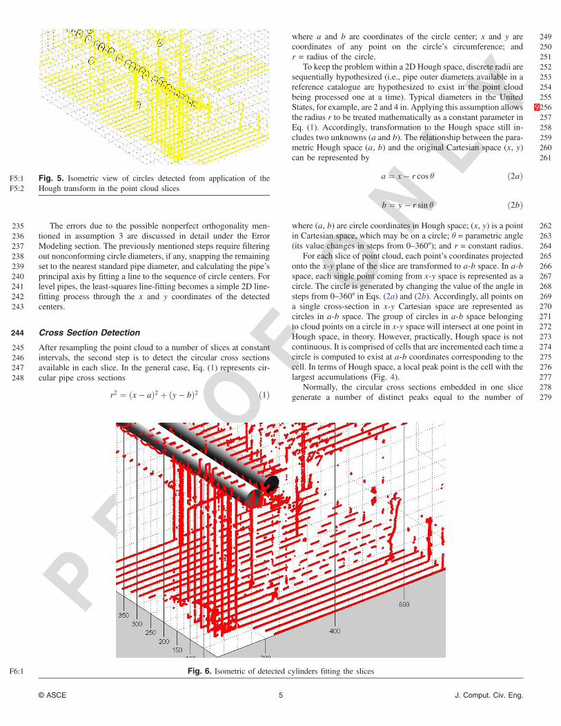
197sections are available, yet they suffice as subsequently described. A198sequential processing of one thin slice per time is applied to detect199the circles of the presumed standard reference radii in each slice200using the Hough transform. In an initial application of this ap-201proach to determine feasibility, a case is examined of pipes along202one corridor under construction.203The proposed technique for recognizing and reconstructing204cylindrical shapes within the 3D point-cloud can be summarized205in the following steps (Fig. 2):206• Resample the original point-cloud to a number of thin separated207slices; slices are chosen at a predetermined interval along the208x-direction, y-direction, and z-direction (Fig. 3);209• For each slice, apply a Hough transform (Fig. 4), and find the210circles satisfying the preknowledge available about the dia-211meters and approximate number of pipes (Fig. 5);212• Connect consecutive centers of detected circles, i.e., grow the213centerlines one interval at a time, and then fit straight lines214through all circles’ centers after processing all the slices; and

F1:1 Fig. 1. Input laser-scan inside the E6 building

F2:1 Fig. 2. Simplified process diagram for detection of cylindrical objects in built-space 3D point-clouds

© ASCE 3 J. Comput. Civ. Eng.

PROOF

ONLY

215 • Construct 3D pipes using computed centerlines and their respec-216 tive radii, then visualize the pipes for confirmation in computer-217 aided design (CAD)8 format on an original full point-cloud, or218 alternatively on the selected slices (Fig. 6).219 Four reasonable premises are then applied to enable efficient220 and practical processing in terms of time, speed, and hardware re-221 sources, as follows:222 1. Some pipes are extended along the corridor under investiga-223 tion (in a more general case, they may change directions224 through 90° elbows);

2252. The pipes are hung above the head of the data-collecting226scanner;2273. Thin slices are selected in nearly perpendicular directions to228the pipes (the error in orthogonality of the slices is within229�6°); and2304. Assume an approximate range about the number of the pipes231in a space and their possible range of discrete diameters for the232facility scanned.233Some or all of the assumptions can be applied as explained in234the Experimental Work section.

F3:1 Fig. 3. Isometric projection of thin slices (in Matlab)

F4:1 Fig. 4. Sample of Hough space voting accumulators (both axes are in centimeters)

© ASCE 4 J. Comput. Civ. Eng.

PROOF

ONLY

235 The errors due to the possible nonperfect orthogonality men-236 tioned in assumption 3 are discussed in detail under the Error237 Modeling section. The previously mentioned steps require filtering238 out nonconforming circle diameters, if any, snapping the remaining239 set to the nearest standard pipe diameter, and calculating the pipe’s240 principal axis by fitting a line to the sequence of circle centers. For241 level pipes, the least-squares line-fitting becomes a simple 2D line-242 fitting process through the x and y coordinates of the detected243 centers.

244 Cross Section Detection

245 After resampling the point cloud to a number of slices at constant246 intervals, the second step is to detect the circular cross sections247 available in each slice. In the general case, Eq. (1) represents cir-248 cular pipe cross sections

r2 ¼ ðx − aÞ2 þ ðy − bÞ2 ð1Þ

249where a and b are coordinates of the circle center; x and y are250coordinates of any point on the circle’s circumference; and251r = radius of the circle.252To keep the problem within a 2D Hough space, discrete radii are253sequentially hypothesized (i.e., pipe outer diameters available in a254reference catalogue are hypothesized to exist in the point cloud255being processed one at a time). Typical diameters in the United256States, for example, are 2 and 4 in. 9Applying this assumption allows257the radius r to be treated mathematically as a constant parameter in258Eq. (1). Accordingly, transformation to the Hough space still in-259cludes two unknowns (a and b). The relationship between the para-260metric Hough space (a, b) and the original Cartesian space (x, y)261can be represented by

a ¼ x − r cos θ ð2aÞ

b ¼ y − r sin θ ð2bÞ

262where (a, b) are circle coordinates in Hough space; (x, y) is a point263in Cartesian space, which may be on a circle; θ = parametric angle264(its value changes in steps from 0–360°); and r = constant radius.265For each slice of point cloud, each point’s coordinates projected266onto the x-y plane of the slice are transformed to a-b space. In a-b267space, each single point coming from x-y space is represented as a268circle. The circle is generated by changing the value of the angle in269steps from 0–360° in Eqs. (2a) and (2b). Accordingly, all points on270a single cross-section in x-y Cartesian space are represented as271circles in a-b space. The group of circles in a-b space belonging272to cloud points on a circle in x-y space will intersect at one point in273Hough space, in theory. However, practically, Hough space is not274continuous. It is comprised of cells that are incremented each time a275circle is computed to exist at a-b coordinates corresponding to the276cell. In terms of Hough space, a local peak point is the cell with the277largest accumulations (Fig. 4).278Normally, the circular cross sections embedded in one slice279generate a number of distinct peaks equal to the number of

F5:1 Fig. 5. Isometric view of circles detected from application of theF5:2 Hough transform in the point cloud slices

F6:1 Fig. 6. Isometric of detected cylinders fitting the slices

© ASCE 5 J. Comput. Civ. Eng.

PROOF

ONLY

280 corresponding pipes, conduit, and ductwork present. However,281 some errors may occur due to noise.

282 Growing the Pipes’ Centerlines

283 Repeating the previously mentioned process on consecutive284 slices, and connecting each new circle’s center to its corresponding285 set in the previous slices, using heuristics subsequently described286 allows the recognized centerlines of the pipes to be grown through287 the slices and the pipes to be reconstructed using their radii288 (Figs. 5 and 6), despite the noise.

289 Modeling the Pipes

290 After processing all slices and the centerlines of all radii of pipes291 are recognized, reconstruction (or modeling) and the drawing292 become the direct next steps. Next, CAD cylinders in point-cloud293 coordinates are generated automatically from the circle sets’ param-294 eters, and are stored as text file data or separately as CAD295 layers (Fig. 6).296 Three additional important issues are discussed further in the297 subsequent sections, as follows: (1) granularity of Hough space,298 (2) degree of confidence, and (3) nonperfect orthogonality299 error-modeling.

300 Granularity of Hough Space

301 Hough space is structured as a 2D voting array in the approach302 described previously. The size of the voting array in Hough space303 can expand or shrink dramatically based on the granularity or tes-304 sellation of the Hough space, which is driven by precision require-305 ments. The choices of granularity applied during the experimental306 work are discussed further in the Experimental Work section.

307 Degree of Confidence

308 As the distance from the scanner station increases, the point-cloud309 density relatively decreases and the noise increases. Conceptually,310 the degree of trust is higher at nearer slices than at farther slices. It is311 possible to formulate this concept approximately as a gradual312 decreasing of confidence as the point-cloud slices increase in accor-313 dance with distance from the scanner station

W ¼ K ×1

Dð3Þ

314 where W = weight (degree of trust); K is a constant; and315 D = distance from the scanner.316 Accordingly, the section S0 nearest to the scanner station is con-317 sidered more trusted than the farthest section Sm. That means that318 during the pipe-growing process, if there is a false circle that was319 voted into the model, the algorithm is able to compare the new320 circle Sn to its preceding accepted circle Sn−1 and also to compare321 it to the very first circle S0, which always has a higher weight. The322 most probable direction is that connecting the preceding accepted323 section Sn−1 and the first section S0. Practically, recognizing the324 first few cross sections including the section nearest to the scanner325 as a start point were enough for a pipe’s centerline recognition.

326 Error Modeling

327 There are many reasons to investigate what types of errors are328 incorporated in applying the proposed technique and finding the329 best way to treat them during processing. This is organized into330 the following research questions:

331• Knowing that perfect orthogonality is not the easiest or default332case, and taking into account the assumption of 6° of possible333deviation from perfect orthogonality, what would be the effect334of tilted slicing of the point cloud?335• What is the effect of the difference between the detected circular336cross section and the elliptical cross section that may result due337to the tilt of the slice?338• What are the types of incorporated errors? What are the signif-339icant error types that need to be taken into consideration, are340there insignificant errors that can be neglected, and to what341degree can each be neglected, if any?342• Are the pipes of small and large diameters affected the same way343by different sources of errors, or does one need to process pipe344categories separately, and if so why?345• What are the effects of pipe diameter and slice sampling interval346on the final model’s precision?347Identification of the error types and derivation of the mathemati-348cal models of the potential effects of nonorthogonality are pre-349sented next.

350Systematic Errors Due to Tilted Cross Sections

351The nonperfect orthogonality of cross sections is a major source of352two systematic errors. Filtering out these errors will enhance the353final localization of the detected cross sections. The first error354comes from the fact that tilted cross sections will be an ellipse.355Hence, in the presence of such systematic error, the cross section356will have one of its diameters larger than the case of the orthogonal357cross section. This effect will shift the center’s position and enlarge358the radius. Accordingly, the center of each cross section will359undergo a systematic displacement (Fig. 7). This displacement360depends on the angle of nonorthogonality. Such an error can be361locally formulated

F7:1Fig. 7. Schematic view showing the shift of center’s position due toF7:2nonperfect orthogonality of the cross section

© ASCE 6 J. Comput. Civ. Eng.

PROOF

ONLY

Rt ¼ R × sec θ ð4Þ362 where θ = tilt angle; R = orthogonal radius; and Rt = tilted radius.363 Thus, the error e1 in the center position is

e1 ¼ Rt − R ð5Þ364365 The second systematic error due to nonperfect orthogonality is366 the shift between any two successive cross sections. This error367 happens in terms of a displacement from one section in one slice368 to the subsequent section in the subsequent slice. It depends on both369 the tilt angle and interval between the two slices (Fig. 8). This error370 e2 can be formulated

e2 ¼ I × tan θ ð6Þ371 where I = interval between any two successive sections.372 Hence, Eq. (6) means that the value of this systematic error in-373 creases if one or both of the following variables increase: (1) inter-374 val distance, and (2) tilt angle. Most significant is a change of the375 angle because it increases in terms of the tangent function of376 that angle.

377 Random Errors

378 The second category of errors is the residual random error e3. This379 is the final residual error, which is accumulated from different ran-380 dom sources such as the effect of temperature, scanned surface381 type, and any instrumental or environmental errors, even truncation382 errors in computations. This error is random and cannot be com-383 pletely represented in one simple mathematical model. The residual384 error changes from one laser scan to another.385 The most probable single residual error e3 at each single cross386 section can be found

e3 ¼ P − Po ð7Þ387 where P = computed best-fitting center’s position; and Po =388 original center’s position after correcting the systematic errors.389 The standard deviation of all cross-section positions along the390 fitted centerline can be estimated

E3 ¼ffiffiffiffiffiffiffiffiffiffiffiffiffiffiffiffiffiffiP

n1 ðe3Þ2n − 1

rð8Þ

391 where E3 = standard deviation of residual errors; and n = number of392 cross sections393 The least-squares line-fitting process computes the best-fitting394 line that minimizes the summation of all the squared values of

395the residual error e3. The least-squares criterion (Mikhail and396Gracie 1981) can be represented

ðe3Þ21 þ ðe3Þ22 þ : : : þ ðe3Þ2n ¼Xn1

ðe3Þ2 → minimum ð9Þ

397398Theoretically, at least two sections are required to be known to399establish the direction. If the length is preknown, the whole pipe400can be reconstructed using the two sections and start point. If401the length is unknown, processing the other slices will be required.402Applying the developed technique provided more redundant data403for the construction of every single pipe. This redundancy en-404hanced the line-fitting process. Due to the high redundancy of405the number of cross sections, satisfying the least-squares criterion406allowed finding the most probable estimation of the best-fitting407line. The final accuracy is detailed in the next two sections.408The answers to all the previous questions, including evaluating409the effect of each error type, and hence categorizing it as either410significant or insignificant, are detailed in the Experimental Work411section. 10Fig. 11 and Tables 1 and 2 summarize a quantitative evalu-412ation of error effects on final results. Application issues are ex-413plored in the next section. Performance is analyzed as well.

414Experimental Work

415Using the FARO 11laser scanner LS 840 HE, data was collected dur-416ing the construction phases of the E6 building on the campus of the417University of Waterloo. The scanner provides a theoretical accuracy418of �3 mm at 20-m distance, with a vertical field-of-view (FOV) of419320° and a horizontal FOVof 360°. It can collect data at a range of4200.6–40.0 m. The recognition and reconstruction of pipe/duct works421installed along the ceiling of each floor from the raw laser-scans422were completed fully automatically using the technique explained423in the previous sections. Software was developed using Matlab on a424typical laptop with the following specs: (1) 8 GB random-access425memory (RAM), and (2) a 1.6 GHz Q 720 processor.426To apply the assumptions mentioned previously in the Proposed427Technique section, several steps were followed. Since pipes are ex-428tended along the corridor or hall under investigation, and the pipes429are hung above the head of the data-collecting scanner, this allows430use of optional spatial constraints on the heights and widths of the431area to be processed at each slice. Tables 1 and 2 compare the effect432of using the optional spatial constraint versus ignoring it. Thin sli-433ces are selected in nearly perpendicular direction to the pipes434(Fig. 3). The slicing process was repeated and evaluated, each time435with a different value of angular nonorthogonality and up to 6° in436steps of 1°. Two ranges of discrete diameters (5–10 and 40–50 cm)437at 1-cm intervals were known in advance and used as input data. It438was assumed that there were 1–10 pipes in each diameter range.439The parametric angle in Eqs. (2a) and (2b) is changed in steps440of 1 or 2°. The developed software allows the visualization of441all computation steps and of the recognized pipes as CAD elements442fitting either the processed slices or a full point-cloud. Fig. 6 dem-443onstrates a sample of results for insulated large diameter pipes.444Fig. 9 demonstrates a case of small-diameter pipes.445A number of important and correlated issues are discussed fur-446ther, as follows: (1) threshold values, (2) applied granularity of447Hough space, (3) processing time, and (4) sequential runs.

448Threshold Values

449To avoid accidental wrong detection of a cross section circle during450the sequential processing of resampled slices, two threshold values451were applied based on experience. The total shift in position

F8:1 Fig. 8. Schematic view of the systematic deviations between anyF8:2 two successive cross sections due to nonorthogonality at an intervalF8:3 of 25 cm

© ASCE 7 J. Comput. Civ. Eng.

PROOF

ONLY

452 between any two successive cross sections must be within the453 following:454 • Two to five cm using low Hough- space granularity, two at 1° tilt455 angle, and five at 6° tilt; this value was suitable for diameters456 around 40–50 cm; and457 • Three to five mm in case of using high Hough-space granularity;458 this value was suitable for diameters around 5–10 cm.

459 Applied Granularity of Hough Space

460 Each cross section covers an area equal to 800-cm wide by 400-cm461 height. For computations up to centimeter-level precision, Hough462 space is represented using 800 × 400 (320,000) cells (bins).463 For computations up to millimeter-level precision, the size of cells464 requires 32 million voting bins in the Hough space corresponding465 to the same slice. Such increases consume magnitudes more466 processing cycles.

467 Processing Time

468 As explained previously, processing the raw millimeter measure-469 ments requires much more cells in Hough space and more time.470 Thus, there are two practical processing scenarios, as follows:471 1. Process all large pipes/ducts using lower-resolution Hough472 space, which requires relatively less time per point-cloud.473 Localization is up to plus or minus a few centimeters. This474 is acceptable in the case of pipes of large diameters and for475 plant operations, but not necessarily for tie-in design.476 2. Use different granulations for the Hough space and use addi-477 tional runs for smaller-diameter pipes, or for localized searches478 in which precision is required.479 A combination of the previous two cases has been applied in the480 research reported in this paper for the following reasons: (1) to gain481 better localization, up to millimeter accuracy; (2) to avoid missing482 any input data, because the pipes of such small diameter have rel-483 atively lower numbers of arc points; and (3) for practicality, it was484 found that dealing with original data accuracy in millimeters is485 enough for localization of the circle center in Hough space to a486 precision of �3–5 mm, provided the systematic errors, especially487 the error e2, are corrected as explained in the Evaluating the Effect488 of Nonperfect Orthogonality section. Based on the preceding

489reasoning, additional runs were performed for pipes of small diam-490eter using a higher resolution of the Hough space.491The processing time for all large pipes/ducts using lower-492resolution Hough space consumed less than 3 min per point cloud493of 40 slices, in which each slice contains 320,000 cells. Processing494the same point cloud for small diameters, in which each slice con-495tains 32 million cells, consumed on average about 10 min per single496run, in which each run dealt with one diameter value only. To cover497the whole range of diameters, 5–10 cm, the whole processing498consumed about 60 min.

499Evaluating the Effect of Nonperfect Orthogonality

500An additional reason for separating the processing of large and501small diameters is the effect of one of the systematic errors, as502explained next.503Figs. 10 and 11 12compare the overall residual error E3 at each tilt504angle for two different groups of pipes versus the common system-505atic errors e1 and e2 in both groups, and up to 6° of tilt. Tables 1 and5062 summarize the accuracy of the investigated technique for the data507set used. Tables 1 and 2 summarize the effect of processing the508complete slice versus constraining Hough-space analysis to certain509spatial zones and preknown diameters on the final output. The510length of the pipe will not be affected if the first and last cross511sections are detected correctly.512Analyzing the experimental results, the following observations513can be made:514• Despite tilted slices causing the detected cross sections to be515elliptical instead of circular, Fig. 11 shows that the actual effect516of this systematic error e1 was the smallest effect among all the517errors. It is less than even the error of the FARO raw data mea-518surements, i.e., less than �3 mm. It is insignificant in the cases519under investigation.520• Based on Eq. (6), the e2 systematic error will increase by in-521creasing either the angle, interval, or both; hence, this is a sig-522nificant error in the cases under investigation. However, the e2523error is constant per interval value and independent of the pipe’s524diameter, and hence e2 is relatively insignificant with very large525pipe diameters like those existing in industrial facilities.526• The standard deviation E3, representing the random error, was527within�5 mm in case of pipes of small diameters, and less than528�1 cm in case of pipes of large diameters. This difference in

F9:1 Fig. 9. Zoom-in to CAD pipe of 5-cm radius fitting the points of two slices

© ASCE 8 J. Comput. Civ. Eng.

PROOF

ONLY

529 value is not due to the size of the diameter as much as it is due to530 the Hough space granularity used in each case. It is not signifi-531 cant in the investigated cases.532 • In the case of diameters of 40–50 cm, the threshold values533 2–5 cm, to accept or reject a newly detected cross section,534 was larger than 3× the standard deviations of random residual

535errors, larger than the combined random and systematic errors,536and larger than maximum residual error for any cross section537position (Fig. 11).538However, in the case of small diameters 5–10 cm, the threshold539values 3–5 mm, were only larger than 3× the standard deviations of540residual errors and the systematic error e1, but not larger than the

F11:1 Fig. 11. Systematic and random errors, deviations from fitting centerline at different nonorthogonal angles (1–6°), units in meters

Table 1. Average Percent of Correct Detected Sections, Constrained versus Nonconstrained Hough Zone Analysis

T1:1 Angle

Nonconstrained Houghzone analysis, without

preknowledge about diameters

Nonconstrained Houghzone analysis, with preknowledge

about diametersConstrained Hough

zone analysis

T1:2 One pipeper time,

5–50 cm (%)

Multiple One pipeper time,

5–50 cm (%)

Multiple One pipeper time,

5–50 cm (%)

Multiple

T1:3 Two pipes,40–50 cm (%)

Three pipes,5–10 cm (%)

Two pipes,40–50 cm (%)

Three pipes,5–10 cm (%)

Two pipes,40–50 cm (%)

Three pipes,5–10 cm (%)

T1:4 1 100 98.5 96.5 100 100 100 100 100 100T1:5 2 100 98 96 100 100 99 100 100 100T1:6 3 100 98 95.5 100 99.5 99.3 100 100 100T1:7 4 100 97 94 100 99 99 100 100 100T1:8 5 99 97 93.5 100 99 98 100 99 99T1:9 6 99 96.5 93 100 98 98 100 99 99

F10:1 Fig. 10. Zoom-in to centerline fitting all cross sections

© ASCE 9 J. Comput. Civ. Eng.

PROOF

ONLY

541 systematic error e2. Thus, it is strongly recommended to remove the542 systematic errors in advance, especially the error e2 in the case of543 small diameters, before testing for rejection or acceptance of a544 newly detected cross section.

545 Discussion of Results

546 For pipe recognition, use of the preknowledge about the installed547 pipes and domain constraints mentioned previously reduced com-548 putational time and cost, because it enabled tracking and growing549 of each group of pipes in one direction in the 3D point-cloud. The550 process can be repeated in more orthogonal directions depending551 on the data set under investigation. The robustness of the presented552 technique is suitable for onsite and office applications. Users or553 developers can optimize the processing strategy based on the ap-554 plication, hardware available, and time available.555 Key advantages of the technique presented in this paper can be556 summarized as follows:557 • It bypasses the need for processing of 5D or greater Hough558 space, hence reducing the overall complexity of the problem559 from a mathematical point of view to a systematic repetitive560 2D Hough space circle-extraction task;561 • One thin slice is processed per time instead of loading and562 processing the complete point-cloud, which at present would563 require special computing facilities, allowing use instead of a564 typical laptop or ordinary PC from a hardware and software565 point of view;566 • Taking into account and filtering out the systematic errors567 enhances the final localization accuracy up to few millimeters568 so that only the insignificant random residuals are affecting the569 results; and570 • Using the appropriate preknowledge, use of such an approach571 can be extended to a broad array of applications and lead to a572 practical cost-effective solution to most of the challenges573 mentioned previously.574 A directly measured comparison to commercial solutions is dif-575 ficult and beyond the means of the researchers given the high cost576 of current commercial solutions. However, a qualitative and ana-577 lytical comparison can be made. Commercial solutions are manual,578 semiautomatic, or automatic to a certain degree. The most recent579 product in today’s market is claiming up to 90% automatic extrac-580 tion of pipes, and it enables the user to manually edit and adjust the581 final output. The editing step is still semiautomatic and requires582 careful visual inspection through the point cloud. Editing in many583 cases requires finding where the pipe sections are missing and then584 drawing a bounding rectangle around each one to help the system to585 recognize it, and in other cases require only mouse clicks within586 each missing section. The revision and editing steps consume some

587processing time and require an experienced technician. The ap-588proach presented in this paper is less dependent on such experience589and the editing step is not required. The presented approach has the590potential to model the as-built status of piping deflection over long591runs, which becomes a significant facility rehabilitation design and592tie-in consideration in practice. Whereas commercial technologies593are advancing as time progresses, most commercial technologies594are still private proprietaries. Hence, more research is required595to fill such gaps.596What has been accomplished at this stage is a validation of the597potential of the general approach. In future research, for cases of598more complex pipe networks, the slicing process is being extended599to three orthogonal directions (x, y, and z), assuming either a range600of possible directions is preknown or searching along the known601angles at standard pipes connections, e.g., 45 and 90°. Generally,602the technique can be applied to recognize pipes in any number of603chosen directions. It depends on the user requirements and avail-604able knowledge about the facility under investigation. Recognizing605true gaps and changes in direction through elbows and tees is an606obvious next step in the research reported in this paper. Standard607complex shapes will be investigated as a combination of multiple608simple elements. Nonlinear noise filters could also be used to re-609duce processing requirements through reducing the number of610points in the point cloud.

611Conclusions

612In the research reported in this paper, a new approach for automatic613detection of cylindrical objects in built facilities was used for614recognition and reconstruction of pipes in a point cloud. Detailed615error-modeling was introduced to filter out the significant system-616atic errors. The final recognition results are promising under the617chosen domain constraints. The level of final localization accuracy618is up to a few millimeters. The technique developed and presented619in this paper reduces computational complexity. It opens a path to-620wards more generic cylindrical shape recognition, modeling and621localization techniques, and a large number of applications. A num-622ber of possible future research extensions have been recommended.623For example, modeling of complex networks of 3D pipes, duct-624work, and conduit is worth pursuing in future research. For625high-accuracy applications, e.g., plant rehabilitation, constrained626least-squares adjustment techniques, and appropriate domain con-627straints can be applied to find the most probable values of all center-628lines of all pipes that best fit all cross sections generated in multiple629directions. More geometric constraints, which can be derived from630available preknowledge, can potentially be utilized to produce a631unique and largely autonomous solution.

Table 2. Average Percentage of Pipe-Growing Length Identified by Growing from Two Scans

T2:1 Angle

One pipeper time,

5–50 cm (%)

Nonconstrained Hough zoneanalysis, without preknowledge

about diameters

Nonconstrained Hough zoneanalysis, with preknowledge

about diametersConstrained Hough

zone analysis

T2:2 Two pipes,40–50 cm (%)

Three pipes,5–10 cm (%)

Two pipes,40–50 cm (%)

Three pipes,5–10, cm (%)

Two pipes,40–50, cm (%)

Three pipes,5–10 cm (%)

T2:3 1 100 97.5 97.5 100 100 100 100T2:4 2 100 97.5 97.5 100 99 100 100T2:5 3 100 97 96 100 99 100 100T2:6 4 100 96.5 95.5 99 99 100 100T2:7 5 100 96 95.5 99 98 100 100T2:8 6 100 95 94 98 98 100 100

© ASCE 10 J. Comput. Civ. Eng.

PROOF

ONLY

632 References

633 Abeid, J., Allouche, E., Arditi, D., and Hayman, M. (2003). “Photo-net II:634 A computer-based monitoring system applied to project management.”635 Autom. Constr., 12(5), 603–616.636 13 Adan, A., Xiong, X., Akinci, B., and Huber, D. (2011). “Automatic creation637 of semantically rich 3D building models from laser-scanner data.”638 Proc., Int. Symp. on Automation and Robotics in Construction, Int. As-639 sociation for Automation and Robotics in Construction, Goyang-Si,640 Republic of Korea, 343–348.641 14 Ahmed, M., et al. (2011a). “Rapid tracking of pipe-works progress using642 digital photogrammetry.” Proc., Construction Specialty Conf.643 15 Ahmed, M., Guillemet, A., Shahi, A., Haas, C., West, J., and Haas, R.644 (2011b). “Comparison of point-cloud acquisition from laser-scanning645 and photogrammetry based on field experimentation.” Proc., Construc-646 tion Specialty Conf., 14–17.647 16 Ahmed, M., Haas, C., and Haas, R. (2011c). “Toward low-cost 3D auto-648 matic pavement distress surveying: The close range photogrammetry649 approach.” Can. J. Civ. Eng., 38(12), 1301–1313.650 Ahmed, M., Haas, C., and Haas, R. (2012). “Using digital photogrammetry651 for pipe-works progress tracking.” Can. J. Civ. Eng., 39(9), 1062–1071.652 Akinci, B., Boukamp, F., Gordon, C., Huber, D., Lyons, C., and Park, K.653 (2006). “A formalism for utilization of sensor systems and integrated654 project models for active construction quality control.” Autom. Constr.,655 15(2), 124–138.656 17 Arachchige, N., Perera, S., and Maas, H. (2012). “Automatic processing of657 mobile laser scanner point-clouds for building façade detection.” Int.658 Arch. Photogramm. Rem. Sens. Spat. Inform. Sci., 34(5), 187–192.18659 19 Bosche, F. (2012). “Plane-based coarse registration of 3D laser scans with660 4D models.” Adv. Eng. Inform., 26(1), 90–102.661 Bosche, F., and Haas, C. T. (2008). “Automated retrieval of 3D CADmodel662 objects in construction 3D images.” J. Autom. Constr., 17(4), 499–512.663 20 Brilakis, I., et al. (2010). “Toward automated generation of parametric664 BIMs based on hybrid video and laser scanning data.” J. Adv. Eng.665 Inform., 24(4), 456–465.666 Cheng, Z., and Liu, Y. (2004). “Efficient technique for ellipse detection667 using restricted randomized Hough transform.” Proc., Int. Conf. on668 Information Technology, Vol. 2, IEEE, New York, 714–718.669 Cheok, G. S., Stone, W. C., Lipman, R. R., and Witzgall, C. (2000). “LA-670 DARs for construction assessment and update.” Autom. Constr., 9(5),671 463–477.672 Chi, S., Caldas, C. H., and Kim, D. Y. (2009). “A methodology for object673 identification and tracking in construction based on spatial modeling674 and image matching techniques.” Comput. Aided Civ. Infrastruct.675 Eng., 24(3), 199–211.676 21 Dai, F., Rashidi, A., Brilakis, I., and Vela, P. (2012). “Comparison of image677 and time of flight based technologies for 3D reconstruction of infra-678 structure.” J. Constr. Eng. Manage.22679 23 Dorninger, P., and Nothegger, C. (2007). “3D segmentation of unstructured680 point clouds for building modeling.” Int. Arch. Photogramm. Rem.681 Sens. Spat. Inform. Sci., 36(3), 191–196.24682 Duda, R. O., and Hart, P. E. (1972). “Use of the Hough transformation to683 detect lines and curves in pictures.” Comm. ACM, 15(1), 11–15.684 El-Omari, S., and Moselhi, O. (2008). “Integrating 3D laser scanning685 and photogrammetry for progress measurement of construction work.”686 Autom. Constr., 18(1), 1–9.687 Golparvar-Fard, M., Bohn, J., Teizer, J., Savarese, S., and Pena-Mora, F.688 (2011). “Evaluation of image-based modeling and laser scanning689 accuracy for emerging automated performance monitoring techniques.”690 Autom. Constr., 20(8), 1143–1155.691 Haas, C. (1986). “Algorithms to map subsurface ferrous conductors.” M.S.692 thesis, Dept. of Civil Engineering, Carnegie Mellon Univ., Pittsburgh.

693Haas, C., and Hendrickson, C. (1991). “Integration of diverse technologies694for pavement sensing.” Transportation Research Record 1311, Trans-695portation Research Board, Washington, DC, 92–102.696Haas, C., Shen, H., Phang, W. A., and Haas, R. (1984). “Application of697image analysis technology to automation of pavement condition sur-698veys.” Proc., Int. Transport Congress, Vol. 5, Balkema, Rotterdam,699Netherlands, C55–C73.700Ibrahim,, Y. M., Lukins,, T. C., Zhang,, X., Trucco,, E., and Kaka,, A. P.701(2009). “Towards automated progress assessment of work package702components in construction projects using computer vision.” Adv.703Eng. Inform., 23(1), 93–103.704Jaselskis, E., Gao, Z., and Walters, R. C. (2005). “Improving transportation705projects using laser scanning.” J. Constr. Eng. Manage., 10.1061/706(ASCE)0733-9364(2005)131:3(377), 377–384.70725Johnson, A. E., and Hebert, M. (1999). “Using spin-images for efficient708multiple model recognition in cluttered 3-D scenes.” IEEE Trans. Pat-709tern Anal. Mach. Intell., 21(5), 433–449.710Kimme, C., Ballard, D., and Sklansky, J. (1975). “Finding circles by an711array of accumulators.” Comm. ACM, 18(2), 120–122.712Kwon, S.-W., Bosche, F., Kim, C., Haas, C. T., and Liapi, K. A. (2004).713“Fitting range data to primitives for rapid local 3D modeling using714sparse range point clouds.” Autom. Constr., 13(1), 67–81.71526Matlab [Computer software]. Natick, MA, MathWorks.71627McLaughlin, J., Sreenivasan, S. V., Haas, C. T., and Liapi, K. A. (2004).717“Rapid human-assisted creation of bounding models for obstacle718avoidance in construction.” J. Comput. Aided Civ. Infrastruct. Eng.,71919(1), 3–15.72028Mikhail, E., and Gracie, G. (1981). Analysis and adjustment of survey mea-721surements, Van Nostrand Reinhold.722Park, H. S., Lee, H. M., Adeli, H., and Lee, I. (2007). “A new approach for723health monitoring of structures: Terrestrial laser scanning.” Comput.724Aided Civ. Infrastruct. Eng., 22(1), 19–30.72529Rabbani, T., and van den Heuvel, F. (2005). “Efficient Hough transform726for automatic detection of cylinders in point clouds.” Proc., Workshop727Laser Scanning, 60–65.72830Rabbani, T., van den Heuvel, F., and Vosselman, G. (2006). “Segmentation729of point clouds using smoothness constraint.” Int. Arch. Photogramm.730Rem. Sens. Spat. Inform. Sci., 36(5), 248–253.731Rashidi, A., Fathi, H., and Brilakis, I. (2011). “Innovative stereo vision-732based approach to generate dense depth map of transportation infra-733structure.” Transportation Research Record 2215, Transportation734Research Board, Washington, DC, 93–99.735Shih, N. J., and Huang, S. T. (2006). “3D scan information management736system for construction management.” J. Constr. Eng. Manage., 10737.1061/(ASCE)0733-9364(2006)132:2(134), 134–142.738Sithole, G., and Vosselman, G. (2003). “Automatic structure detection in a739point-cloud of an urban landscape.” Proc., Joint Workshop on Remote740Sensing and Data Fusion over Urban Areas, IEEE, New York, 67–71.741Tang, P., Huber, D., Akinci, B., Lipman, R., and Lytle, A. (2010). “Auto-742matic reconstruction of as-built building information models from laser-743scanned point clouds: A review of related techniques.” Autom. Constr.,74419(7), 829–843.745Teizer, J., Caldas, C. H., and Haas, C. T. (2007). “Real-time three-746dimensional occupancy grid modeling for the detection and tracking747of construction resources.” J. Constr. Eng. Manage., 10.1061/748(ASCE)0733-9364(2007)133:11(880), 880–888.74931Vosselman, G., and Dijkman, S. (2001). “3D building model reconstruction750from point clouds and ground plans.” Int. Arch. Photogramm. Rem.751Sens. Spat. Inform. Sci., 37–44. 32752Wu, Y., Kim, H., Kim, C., and Han, S. H. (2010). “Object recognition in753construction-site images using 3D CAD-based filtering.” J. Comput.754Civ. Eng., 10.1061/(ASCE)0887-3801(2010)24:1(56), 56–64.

© ASCE 11 J. Comput. Civ. Eng.