1   

                                                                                 

VIBRATION ANALYSIS OF A THIN

CYLINDRICAL SHELL

A thesis submitted to the department of Mechanical and Chemical Engineering (MCE), Islamic University of Technology (IUT), in the partial fulfillment of the requirement for

the degree of Bachelor of Science in Mechanical Engineering.

Prepared by:

MD. AKIBUL ISLAM (101439)

AHMED NIRJHAR ALAM (101441)

Supervised by:

Dr. MD. ZAHID HOSSAIN

Mr.SHAHRIAR ISLAM

Department of Mechanical and Chemical Engineering

Islamic University of Technology

2   

Organization of Islamic Cooperation (OIC)

Declaration

This is to certify that the work presented in this thesis is an outcome of the experiment

and research carried out by the authors under the supervision of Dr. Zahid Hossain and

Mr.Shahriar Islam.

Signature of the Candidates

________________ _________________

Md.Akibul Islam Ahmed Nirjhar Alam

(Author) (Author)

Date: Date:

Signature of the Supervisors

3   

Dr. Md. Zahid Hossain

(Assistant Professor)

(Project Supervisor)

Date:

Mr.Shahriar Islam

(Lecturer)

(Project Supervisor)

Date:

ACKNOWLEDGEMENT

All praises to Almighty ALLAH (Sbw) who blessed us with potential and patience to

complete this project successfully overcoming the obstacles in the way.

It is not sufficient to only give thanks to some people who helped and guided us when

needed and without them the thesis could never come into being successfully in time.

Our gratitude and respect to our supervisors Prof. Dr. Md. Zahid Hossain and

Assistant Prof. Mr.Shahriar Islam, MCE Department, Islamic University of

Technology(IUT) for their encouragement, erudite advices and extreme patience

throughout the course for establishing such a creative project. Their care, concern and

continuous moral support for the students are appreciated.

We are also grateful to the Head of Mechanical and Chemical Engineering Department

Dr. Md. Abdur Razzaq Akhanda for providing us with necessary funding and supports.

Special thanks to Md Rakibul Hasan (mechanics lab) for his useful suggestions and

availability whenever needed.

4   

We would also like to give thanks to all faculty members of the department for their

advice and support throughout the project. All of us are indebted to our family members

for their moral supports and prayers.

Although we tried our best to complete this thesis flawlessly, we seek apology if there is

any mistake found in this report.

ABSTRACT

In this paper, vibration characteristics of thin cylindrical shell are investigated by using

& ANSYS WORKBENCH 14.0. Vibration response are investigated by Transient

Structural analysis for the simply supported boundary conditions. It is also necessary to

investigate the characteristics considering fluid-structure interaction (FSI) effect by

System Coupling between Transient structural and Fluent flow. In this study, theoretical

background and several finite element models are developed for cylindrical shells with

fluid-filled annulus considering fluid-structure interaction. The effect of the inclusion of

the fluid-filled annulus on the natural frequencies is investigated, which frequencies are

used for typical dynamic analyses the equations of motion of the structure for the

theoretical analysis are obtained from Love’s equation.

5   

TABLE OF CONTENTS

CHAPTER-1: INTRODUCTION…………………………………………………………..7-9

LITERATURE REVIEW……………………………………………..……………………………………….. 8

CHAPTER-2: BASICS OF VIBRATION…………………………………………….10-15 TYPES OF VIBRATION ………………………………………………………………………………10-12

STEADY STATE VIBRATION OR RESPONSE……………………………………………….12-13

THIN-WALLED CYLINDER………………………….………………………………………………13-14 RESONANACE………………………………………………………….………………………………………..14 TRANSIENT ANALYSIS………………………………………………………………………….…….14-15 FLUID-STRUCTURE INTERACTION ……………………………..…………………………….15-16 CHAPTER-3: NUMERICAL ANALYSIS FOR DETERMINATION OF AMPLITUDE & FREE VIBRATION RESPONSE OF A CIRCULAR CYLINDRICAL SHEL…………………………………………………………………………………….……..16-46 NUMERICAL ANALYSIS……………………………………………………………………………..16-17 TRANSIENT ANALYSIS………………….………………………………………………………………….17 TRANSIENT RESULT………….……………………………………………………..…………………30 FLUID-STRUCTURE INTERACTION………………………………………………………………….31 SYSTEM COUPLING…………………………………………………………………………………………..39 FSI RESULT…………..……………………………………………………………………………………44-45

6   

CHAPTER 4: ANALYTICAL ANALYSIS FOR DETERMINING VIBRATION

RESPONSE OF A THIN CYLINDRICAL SHELL .………………………..…………...46-55

STRESS-STRAIN RELATIONSHIP…………………………….…………………………………………51

NEWTON-RAPHSON METHOD………………………………..………………………..……………… 53

CHAPTER-5: EXPERIMENTAL ANALYSIS FOR DETERMINING NATURAL FREQUENCIES AND FORCED VIBRATION RESPONSE CIRCULAR CYLINDRICAL SHELL…………………………………………..……..55-60 EQUIPMENTS …………………………………………..………………………………………………….….. 55 PROBLEM SPECIFICATIONS……………………………………………………………………………...55 DESCRIPTION OF THE PROXIMITY SENSOR………………………………………………56-60 EXPERIMENTAL SETUP…………………………………………………………..…….……………..…..60

7   

CHAPTER 1

INTRODUCTION

Thin walled cylindrical shells are very often in the field of engineering applications.

Shell structures are common especially in spacecraft, aircraft, shipbuilding and

automotive industries. They are also used as oil and gas carrying pipelines. Present day

sees a great increase in the applications of cylindrical shells in the form of structural

components for pressure vessels, process equipment’s, missiles, rockets and civil

engineering constructions. Most of the failures occurring in these structures are due to

dynamic loading. For instance, the infamous tragic failure of NASA space shuttle

CHALLENGER on 20th January, 1986 was mainly due to structural failure. That’s why

vibration analysis of shell structures has been of great importance for last few decades.

The natural frequencies and mode shapes are important sources of information for

understanding and controlling the vibration of these structures.

Such cylindrical structures are often subjected to dynamic loading. Such as the flow-

induced vibrations in heat exchangers and pipelines, wave-loading on submarines, the

impact-loading of vehicles, the aero-elastic flutter of aircrafts, vibrations of

underground and under-sea pipe- lines and certain defense-related equipment.

Vibrations in the aforementioned pipelines are generally caused by external driving

agencies such as earthquakes, nuclear and other explosions, wave-loadings, superfast

trains and super-sonic jets. Thin-walled structures are very prone to resonant vibrations

because their Eigen frequencies lie in a very narrow band. So it is essential for the

designer to know the distribution of Eigen frequencies of the proposed structure

beforehand.

Therefore main focus of our work was to observe the behavior of a thin walled

cylindrical shell (Transient structural analysis) at various end conditions and observe

the Fluid-Solid interaction effect for inside fluid flow.

8   

This analysis consists of three phases namely Numerical Analysis, Analytical analysis

and experimental analysis. In numerical analysis ANSYS (workbench 14.0) was used to

observe the response of thin cylindrical shell (Transient Analysis) and for inside fluid

flow system coupling was used to observe solid-fluid interaction effect. In analytic

analysis the Love’s approach was used to find the equations of motions and then the

eigenvalues were calculated. For experimental analysis an inductive proximity sensor

was used to find natural frequency of the shell.

LITERATURE REVIEW

As we have already known the importance of shell structure analysis from the

introduction before, now we’ll look into various shell theories those have paved the way

to the present day extensive shell analysis.

Regarding researches of shell vibration, Leissa [1] has collected most of the results before

1973. Chung [2] and Greif and Chung [3] used the Rayleigh-Ritz method, for different

boundary conditions, to find the natural frequencies. Sharma and Johns [4, 5] and

Goldman [6] calculated the natural frequencies and modes for free and fixed boundary

conditions. Stoke’s transformation technique was applied by Chung [7] to solve the

natural frequencies for different boundary conditions. Mnev and Pertsev [8], Junger and

Feit [9] ,and Brown [1O] have done some research on vibration of shells with the

interaction of internal fluid. Chu etel. [11] Used the energy method to obtain the

frequency parameters. Recent works include Conclaves’ [12] investigation of non-linear

vibrations of thin-walled cylinders with liquid interaction.

Markus [13] has provided an extensive analysis of cylindrical shells using membrane as

well as bending theory. He has discussed the cons and pros of the membrane theory. He

discussed various shell theories due to Donnell-Mushtari, Love-Timoshenko, FlÜgge,

Sander etc.

In recent years Bert et al. [14] have given an analytical solution to the free vibration of a

composite material cylindrical shell with ring and stringer stiffeners and compared the

9   

numerical values given by various shell theories, by the use of dimensionless tracer

coefficients. Mustafa and Ali [15-17] have predicted natural frequencies of stringer

stiffened and ring stiffened cylindrical shells using semi-loof and facet shell finite

elements on half and quarter models of the shells, because of structural symmetry. They

have compared the numerical values obtained by them, with the experimental values of

Hoppmann [18].They have also given an energy method to study the natural frequencies

of externally and internally stinger stiffened cylindrical shells and ring stiffened shells.

Rinehart and Wang [19, 20] have investigated the free vibration characteristics of Simply-

supported cylindrical shells stiffened by discrete longitudinal stiffeners using energy

method. They have compared the numerical values given by the more exact F’lugge’s

theory and Donnell’s approximate theory and shown that Donnell’s approximate theory

gives excellent results for the stiffened shells.

Previous studies confirmed that the effect of shear deformation can become quite

significant for small radius-to- thickness or length-to-thickness ratios, as well as for

shorter wavelengths of longer shells [21]. More recently, Bhimaraddi [21] developed a two-

dimensional (2-D) higher-order shell theory for free vibration response of isotropic

circular cylindrical shell and assumed the inner and outer surfaces of the shell to be

traction free. Also, Reddy and Liu [22] presented a 2-D higher-order theory for laminated

elastic shells.

10   

CHAPTER 2

BASICS OF VIBRATION

TYPES OF VIBRATION

FREE AND FORCED VIBRATION

FREE VIBRATION

After an initial disturbance, if a system is left to vibrate on its own then it is called free

vibration. In free vibration no external force is applied or acted on the system.

Oscillation of a simple pendulum is an example of free vibration.

FORCED VIBRATION

If a system is subjected to an external force (often repeating types) the resulting

vibration is known as forced vibration. The oscillation that arises in machine. Such as

diesel engine is an example of forced vibration.

UNDAMPED AND DAMPED VIBRATION

UNDAMPED VIBRATION

During oscillation if no energy is lost or dissipated due to friction or other resistances

then the vibration is known as undamped vibration. In an undamped vibration the

magnitude of amplitude is not changing with time.

11   

Figure: undamped vibration

DAMPED VIBRATION:

During oscillation if energy is lost due to friction or other resistances then it is called

damped vibration. During damped vibration the magnitude of amplitude or

displacement is changed with time.

Figure: Damped vibration

LINEAR VIBRATION AND NONLINEAR VIBRATION:

LINEAR VIBRATION:

12   

If all basic components of a vibratory system –the spring, the mass, and the damper

behave linearly, the resulting vibration is known as the linear vibration. If the vibration

is linear then the principle of superposition holds.

NONLINEAR VIBRATION:

If any of the basic components of vibration behave nonlinearly then the vibration is

called nonlinear vibration. For nonlinear vibration the principle of superposition is not

valid.

STEADY STATE VIBRATION OR RESPONSE

At forced vibration the system will tend to vibrate at its own natural frequency and to

follow the frequency of the external force applied. In the presence of friction the portion

of motion not sustained by the excitation force will gradually die out. In other words due

to friction the tendency of vibrating at natural frequency will be eliminated. As a result

the system will vibrate at the frequency of external force only regardless of the initial

conditions or the natural frequency of the system. This part of sustained vibration is

called the steady state vibration or response of the system. Very often the steady state

response is required in vibration analysis because of its continuous effect.

13   

Figure: steady state vibration

THIN –WALLED CYLINDER

For the thin-walled assumption to be valid the vessel must have a wall thickness of no

more than about one-tenth (often cited as one twentieth) of its radius. This allows for

treating the wall as a surface, and subsequently using the Young–Laplace equation for

estimating the hoop stress created by an internal pressure on a thin wall cylindrical

pressure vessel:

Where,

14   

RESONANCE

A certain system has more than one natural frequency. If the frequency of the external

force coincides with one of the natural frequencies of the system, a condition known as

resonance occurs. When resonance happens, the amplitude of vibration will increase

without bound and is governed only by the amount of damping present in the system

and the system undergoes dangerously large oscillations. Therefore, in order to avoid

disastrous effects resulting from very large amplitude of vibration at resonance the

natural frequency of a system must be known and properly taken care of. Otherwise

failures of such structures as buildings, bridges, turbines and airplane wings may be

occurred.

 

Figure: resonance curve

TRANSIENT ANALYSIS:

Transient Structural analysis is used to determine the dynamic response of a structure

under the action of any general time-dependent loads. it is used to determine the time-

15   

varying displacements, strains, stresses, and forces in a structure as it responds to any

transient loads. The time scale of the loading is such that the inertia or damping effects

are considered to be important. If the inertia and damping effects are not important, it

might be able to use a static analysis instead.

A transient structural analysis can be either linear or nonlinear. All types of

nonlinearities are allowed - large deformations, plasticity, contact, hyper elasticity and

so on. In the Mode Superposition method, the transient response to a given loading

condition is obtained by calculating the necessary linear combinations of the

eigenvectors obtained in a modal analysis.

FLUID-STRUCTURE INTERACTION:

Fluid–structure interaction (FSI) is the interaction of some movable or deformable

structure with an internal or surrounding fluid flow. Fluid–structure interactions can be

stable or oscillatory. In oscillatory interactions, the strain induced in the solid structure

causes it to move such that the source of strain is reduced, and the structure returns to

its former state only for the process to repeat.

FLUID STRUCTURE INTERACTION ANALYSIS:

Fluid–structure interaction problems and multiphysics problems in general are often

too complex to solve analytically and so they have to be analyzed by means of

experiments or numerical simulation. Research in the fields of computational fluid

dynamics and computational structural is still ongoing but the maturity of these fields

enables numerical simulation of fluid-structure interaction. Two main approaches exist

for the simulation of fluid–structure interaction problems:

• Monolithic approach: the equations governing the flow and the displacement of

the structure are solved simultaneously, with a single solver

• Partitioned approach: the equations governing the flow and the displacement of

the structure are solved separately, with two distinct solvers

16   

The monolithic approach requires a code developed for this particular combination of

physical problems whereas the partitioned approach preserves software modularity

because an existing flow solver and structural solver are coupled. Moreover, the

partitioned approach facilitates solution of the flow equations and the structural

equations with different, possibly more efficient techniques which have been developed

specifically for either flow equations or structural equations. On the other hand,

development of stable and accurate coupling algorithm is required in partitioned

simulations

CHAPTER 3

NUMERICAL ANALYSIS FOR DETERMINING FREE VIBRATION

RESPONSE OF A THIN CIRCULAR CYLINDRICAL SHELL

NUMERICAL ANALYSIS

Numerical analysis is the study of algorithms or step by step process that use numerical

approximation (as opposed to general symbolic manipulations) for the problems of

mathematical analysis (as distinguished from discrete mathematics).

A numerical method which leads to a required result is often referred to as an algorithm. More often than not, algorithms are iterative, i.e., they involve cycles of identical

17   

computations, starting with the results of the preceding cycle. At the end of a cycle, the result will be examined to find out whether it has the required accuracy. The algorithm will stop, when the error becomes as small as desired

USE OF ANSYS IN TRANSIENT STRUCTURAL ANALYSIS

The general process for a Transient structural analysis involves following primary steps:

1. Engineering data.

2. Create Geometry.

3. Model.

4. Set up.

5. Solution.

6. Results.

ANSYS SIMULATION OF A CYLINDRICAL SHELL

Now the process described above will be applied for a cylindrical shell to analyze its transient response.

PUTTING ENGINEERING DATA FOR CYLINDRICAL SHELL IN ANSYS WORKBENCH 14.0

Firstly,Select Engineering data

Then create new material with following properties:

• Young’s Modulus : 2.5E+011 Pa • Poison’s Ratio : 0.3 • Density : 7850kg/m^3

18   

After that,select this as Default Material for Solid

Secondly,select Geometry and draw a rectangle of 80mm*80mm on the XY plane

19   

After that,draw two circles of radius 59mm and 53.8mm at the center of the rectangle.Extrude the whole drawing 2200mm.Then from the toolbar,FREEZE it.

Now freeze it from toolbar.

Then select new sketch………

20   

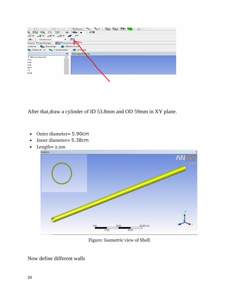
After th

Now de

hat,draw a c

efine differ

cylinder of

rent walls

f ID 53.8mmm and ODD 59mm inn XY plane

 

e.

21   

1. Wall inlet and outlet:The wall inlet is shown here.Opposite side is wall outlet.Select the face,right click and select NAMED SELECTION.Give name Wall inlet and GENERATE.

2. Wall top and bottom: The Wall top is shown.the bottom part is Wall bottom.

3. Side 1 & side 2: Side 1 is shown.Side 2 is exactly the opposite face.The Side 1 is 80mm from the origin.

22   

4. Wall Deforming:

23   

Now SAVE the geometry file.

1.TRANSIENT ANALYSIS WITH NO STRUCTURAL DAMPING/WITH DAMPING AND NO FLUID PRESENCE:

Select the MODEL from Transient Structural.

Input all necessary data required for Transient Structural Analysis such as analysis settings,displacement,force,fluid solid interface.For Meshing,suppress the Fluid portion.

• Analysis settings: For the Analysis settings- Select Step End Time : 3s Auto Time Stepping : OFF Time Step : 0.01s

24   

 

 

 

 

 

• D

For tsupp

Displaceme

the displacported:

ent: 

cement of tthe two endds if the cy

 

ylinder,as tthey are simmply

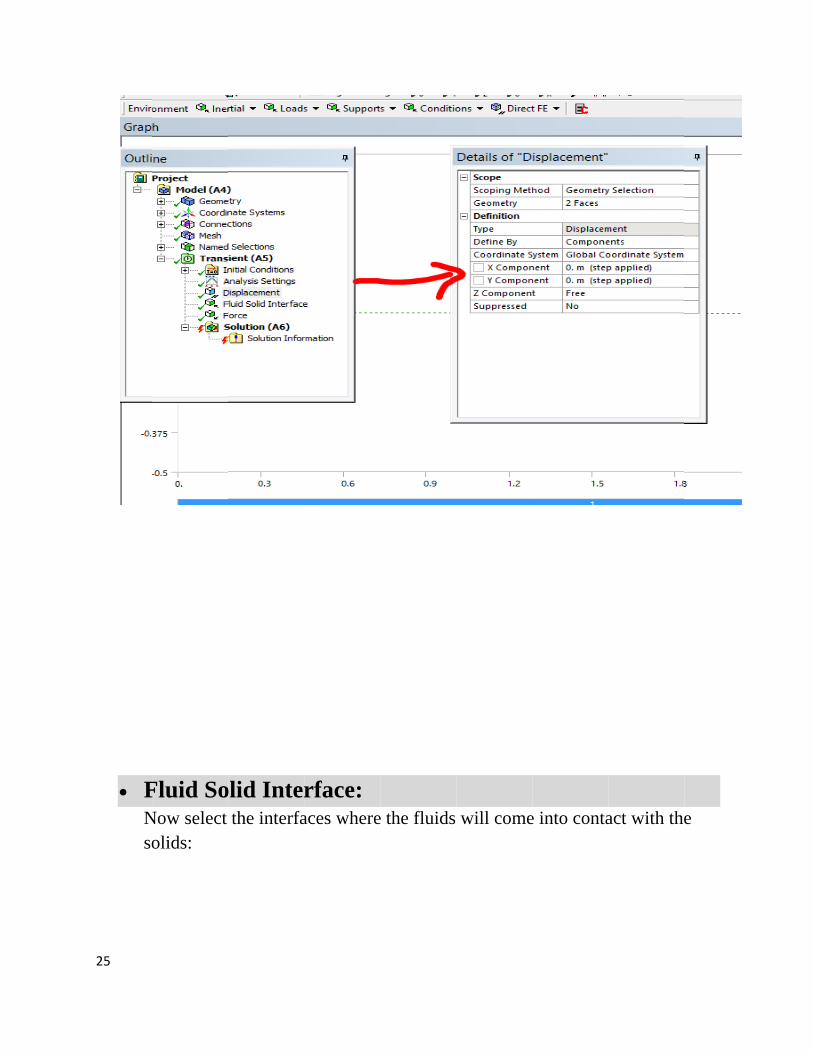
25   

• F

Nso

Fluid SoNow select olids:

olid Interthe interfa

rface: aces wheree the fluids will comee into contaact with the

e

26   

• F AdWM

For Force:

As force is direction anWe will useMESH SEL

applied fornd release ie Nodal FoLECT to S

r a small tiit after 0.0orce.So,firSELECT a

ime,here w1 second.rst select ma box of re

we use 30N

mesh from tegion.

N force in d

the Outlin

downward

ne.Then use

e

27   

T

In

Then Create

nsert Noda

e a Named

al Force in

d Selection

n the TRAN

n of the sele

NSIENT(A

ected box m

A5) section

mesh.

n.

28   

T

The magnittude of forcce is as bellow:

29   

Incp

Afoe

nsert TOTlick on the

presence of

As there is norever.Butfficient of

TAL DEFOe Solution af fluid,the r

no dampint by manuaMild Steel

ORMATIOand select result is as

ng the vibraal calculatiol is 0.2.Run

ON in the SOLVE.Wbelow:

ation will bon,we founnning the S

“SOLUTIWithout Str

be Steady nd out thatSimulation

ION(A6)” ructural Da

State and ct the dampin again usin

secton.Rigamping and

continue ing co-ng this val

ght d no

lue:

30   

There is a significant change in vibration characteristic due to structural damping. The modal shapes of vibration:

31   

1. FLUID STRUCTURE INTERACTION USING DIFFERENT FLUIDS:

For the simulation of Fluid-Structure Interaction Transient Structural &

Fluid Flow (Fluent) need to be taken from the workbench’s Analysis System.

Then the geometry of Transient Structural has been linked up with the geometry

of Fluent by dragging into one another.

To insert the geometry it is needed to make a model for fluid flowing inside the

shell. And it is done by using Design Modeler.Now open the MESH of

FLUENT.Suppress the solid body and generate MESH.

32   

Open SETUP from FLUENT.

Now for setting up first select

Option> double precision

Processing Option> Serial, Then OK.

Now, for fluid flow (Fluent) setup follow the steps: General>

33   

We are working with only laminar flow.So Select Models and follow the steps

34   

Select Materials and define the density.Air density is put automatically.

Defining Dynamic Mesh:

A dynamic mesh is needed for any coupled analysis where a system receives

displacements.The mesh on the fluid-structure interface is static,so as the

fluid mesh is modified to accommodate the deformation in the transient

system,the mapping on this coupling interface stays constant.

35   

On the left,select Solution setup>Dynamic mesh

Under Mesh Methods,Smoothing is checked by default.Click the

Settings button to specify the setting for the smoothing method.

The Mesh Method Settings dialog box appears.

a. On the Smoothing tab,Set method to Diffusion.

b. For the Diffusion Parameter,type 2.Click OK to close the

Mesh Method Setting dialog

36   

Under Dynamic Mesh Zones,click Create/Edit to specify which

zones in the geometry will have dynamic meshing.The Dynamic

Mesh Zone dialog box appears.

Define the Dynamic Mesh Setting Needed for the surface “Side

1”,which is the wall in the X-Y plane.

a. In the Dynamic Mesh Zone dialog box,under the Zone

Names drop dpwn list,select the zone “side 1”

b. Set its type as Deforming.

c. Select the Geometry Definition tab.

d. Specify Definition as “plane”

e. Specify Point On Plane as “0.08,0,0”

f. Specify Plane Normal as “1,0,0”

g. Click Create at the bottom.

Similar process is done for “Side 2”.Only exception is Point On

The Planes will be “0,0,0”

Under the Zone Names drop down list,select the zone “wall

bottom”.Set its TYPE as Stationary,then click Create at bottom.

Repeat the process for “wall top”,”wall inlet”,”wall outlet”

Now from the Zone Names drop down,select “wall deforming”

and set its type as System Coupling.

Now close the box.

37   

Adding the Solution Setting:

On the left side of Fluent Application,select Solution>Solution

Methods.Under Pressure-Velocity Coupling>Scheme,select

Coupled.Under Spatial Discretization>Momentum,select Second

Order Upwind.

38   

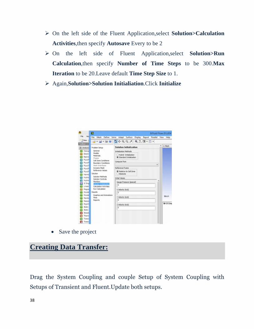
On the left side of the Fluent Application,select Solution>Calculation

Activities,then specify Autosave Every to be 2

On the left side of Fluent Application,select Solution>Run

Calculation,then specify Number of Time Steps to be 300.Max

Iteration to be 20.Leave default Time Step Size to 1.

Again,Solution>Solution Initialiation.Click Initialize

• Save the project

Creating Data Transfer:

Drag the System Coupling and couple Setup of System Coupling with

Setups of Transient and Fluent.Update both setups.

39   

A. In Outline Schemetic C1:System Coupling,expand System

Coupling>Setup>Participants until all region components are visible.

B. Ctrl-select the “wall deforming” and “Fluid-solid interface”

regions.With both selected,right-click on one of these regions and

select “Create Data Transfer”.Under System Coupling>Setup>Data

Transfer.

Preparing System Coupling for Restarts:

i. Under System Coupling>Setup>Execution Control,select

Intermediate Restart Data Output.The restart output frequency for the

system coupling analysis is defined and controlled by these settings.

ii. In Properties of Intermediate Restart Data Output:

• Set Output Frequency to At Step Interval

• Set Step Interval to 5

Select File>Save

Solving:

Right-click on Solution and select update.

40   

Results:

Open the Result window to view the result.

Go to Insert Menu>Location>Point.

Click OK for the default name “Point 1”.

In the detail of Point 1, set the Domains as “Default domain” & set the method as

XYS. Then select the suitable node.-

Then insert the X,Y,Z co-ordinates as .04,.095 and -1.1 respectively.

41   

Again go to “Insert Menu”> Chart. Then click OK to the default name “Chart 1”

In Detail of chart 1,

General > Type >XY transient or sequence.

42   

Data series > Location, Select “Point 1”.

X Axis > Expression > Time >Axis range > Deselect “Determine Range

Automatically” Then put suitable Min & Max values.

43   

Y Axis > Expression > Total displacement Y>Axis range > Deselect “Determine

Ranges Automatically”> select suitable Min & Max values.

Finally Click Apply.

44   

The Result for FSI using AIR :

Fig: Fluid-Structure Interaction effect with AIR

Maximum amplitude of vibration is 0.13 mm

45   

The result or FSI using WATER:

Fig:Fluid-Structure Interaction effect using WATER

The maximum amplitude of vibration is 3E-05 mm.

46   

CHAPTER 4

ANALYTICAL ANALYSIS FOR DETERMINING

VIBRATION RESPONSE OF A THIN CYLINDRICAL SHELL

In this chapter, we will look into a mathematical approach, as described by Werner

Soedel in the book titled “Vibrations of Shells and Plates, Third Edition” to find out

Transient response of a simply supported circular cylindrical shell and see that how

the structure responds when fluid is flowing through the cylindrical shell. For that,

equations of motion for the shell are needed which requires a way to relate the

motion of the structure to the loads acting on it. This is done by first developing

relationships between stress and strain, as strain is technically deformation of the

body so stresses can be related to displacement of the structure which again warrants

for the relationships between strain and displacement.

Both the Newton–Raphson method and fixed-point iteration can be used to solve

FSI problems. Methods based on Newton–Raphson iteration are used in both the

monolithic and the partitioned approach. These methods solve the nonlinear flow

equations and the structural equations in the entire fluid and solid domain with the

Newton–Raphson method. The system of linear equations within the Newton–

Raphson iteration can be solved without knowledge of the Jacobian with a matrix-

free iterative method, using a finite difference approximation of the Jacobian-vector

product.

47   

SHELL COORDINATES AND INFINITESIMAL DISTANCES

IN SHELL LAYERS

Here we will assume that thin, isotropic, and homogeneous shells of constant

thickness have neutral surfaces, just as beams in transverse deflection have neutral

fibers. Stresses in such a neutral surface can be of the membrane type but cannot be

bending stresses. To locate any point on the neural surface of the shell we will use

curvilinear coordinate system. The location of point P on the neutral surface in three

dimensional Cartesian coordinates can be expressed by two dimensional curvilinear

surface coordinates as follows,

The location of P on the neutral surface can also be expressed by a vector,

48   

Fig 1. Reference surface

Now the infinitesimal distance between points P and P′ on the neutral surface is

the differential change, dr of the vector from P to P′,

(3)

The magnitude “ds of is given by

Simplifying this, we get,

This equation is called the “fundamental form” and A1 & A2 are the “fundamental

form parameters” or “Lamé parameters”.

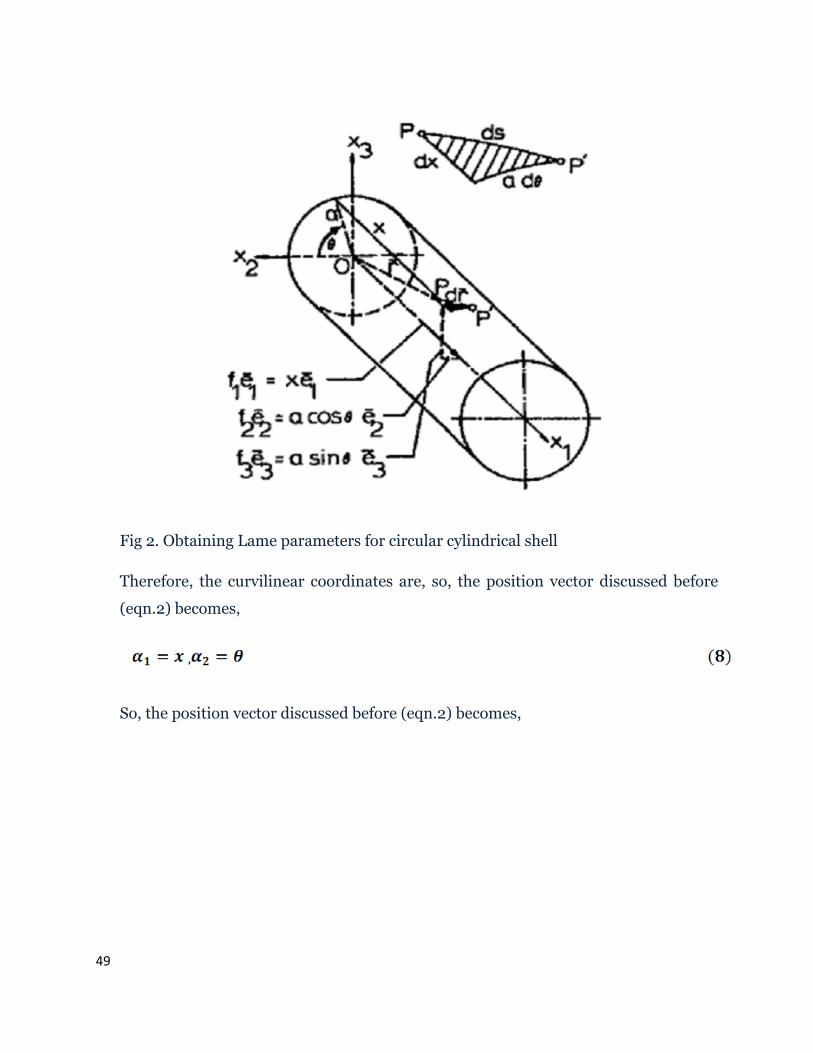
Now being specific to our structure of interest i.e. circular cylindrical shell, for each

point on shell surface there are two maximum and minimum radius of curvature,

whose directions are perpendicular to each other. These lines of principal curvature

are in this case parallel to the axis of revolution, where the radius of curvature Rx=∞

(i.e. curvature 1/Rx=0) and along the circles,

49   

Fig 2. Obtaining Lame parameters for circular cylindrical shell

Therefore, the curvilinear coordinates are, so, the position vector discussed before

(eqn.2) becomes,

So, the position vector discussed before (eqn.2) becomes,

50   

Recognizing that the fundamental form can be interpreted as defining the

hypotenuse ds of a right triangle whose sides are infinitesimal distances along the

surface coordinates of the shell, we may obtain A1, and A2 in a simpler fashion by

expressing ds directly using inspection:

By comparison with eqn.3, we get,

Now let us define coordinate to be perpendicular to plane i.e. for circular

cylindrical shell it is the normal direction to the undeflected shell surface and is 0 on

neutral plane. If P1 and P1′ are two points on different planeswhose projections on

the neutral surface are at infinitesimal distance, then the distance between these two

points, ds can be derived by similar mathematical approach to be,

Where, R1 and R2 are radius of curvatures.

This equation gives the distance between two points of an undeflected shell.

51   

STRES

Acco

perp

appli

We w

that,

SS-STRA

ording to t

endicular p

ies, therefo

will later as

AIN RELA

the coordin

planes of st

re we have

ssume that t

ATIONS

nate system

train and th

for a three

transverse

SHIP

m we hav

hree shear s

dimension

shear defle

e chosen,

strains. We

nal element.

ections can

we have

e assume th

.

be neglecte

three mutu

hat Hooke’s

ed. This im

ually

s law

mplies

52   

The n

will b

This

acts o

is a r

load

Our e

normal stre

be neglecte

is because

on the shel

relatively sm

do we reac

equation sy

F

ess, which

d,

we argue t

l, it is equiv

mall value

ch magnitud

ystem there

Fig 3.Stresse

acts in the

that on an u

valent in m

in most ca

des that wo

efore reduce

es acting on

normal dir

unloaded o

agnitude to

ses. Only in

ould make t

es to,

n an elemen

rection to th

outer shell s

o the extern

n the close

the conside

nt

he neutral s

surface it is

nal load on

vicinity of

eration of

surface,

s 0, or if a f

the shell, w

f a concentr

worthw

force

which

rated

while.

53   

Only the first three relationships will be of importance in the following. Equation

(29) can later be used to calculate the constriction of the shell thickness during

vibration, which is of some interest to acousticians since it is an additional noise

generating mechanism, along with transverse deflection.

Newton–Raphson method

Newton–Raphson methods solve the flow and structural problem for the state in the

entire fluid and solid domain, it is also possible to reformulate an FSI problem as a

system with only the degrees of freedom in the interface’s position as unknowns.

This domain decomposition condenses the error of the FSI problem into a subspace

related to the interface.[7] The FSI problem can hence be written as either a root

finding problem or a fixed point problem, with the interface’s position as unknowns.

Interface Newton–Raphson methods solve this root-finding problem with Newton–

Raphson iterations, e.g. with an approximation of the Jacobian from a linear

reduced-physics model. The interface quasi-Newton method with approximation for

the inverse of the Jacobian from a least-squares model couples a black-box flow

solver and structural solver [10] by means of the information that has been gathered

during the coupling iterations. This technique is based on the interface block quasi-

Newton technique with an approximation for the Jacobians from least-squares

models which reformulates the FSI problem as a system of equations with both the

interface’s position and the stress distribution on the interface as unknowns. This

system is solved with block quasi-Newton iterations of the Gauss–Seidel type and

54   

the Jacobians of the flow solver and structural solver are approximated by means of

least-squares models.

The fixed-point problem can be solved with fixed-point iterations, also called (block)

Gauss–Seidel iterations, which means that the flow problem and structural problem

are solved successively until the change is smaller than the convergence criterion.

However, the iterations converge slowly if at all, especially when the interaction

between the fluid and the structure is strong due to a high fluid/structure density

ratio.

The Newton Raphson method is for solving equations of the form f(x) = 0. We make an

initial guess for the root we are trying to find, and we call this initial guess x0.The

sequence x0, x1, x2, x3, . . . generated in the manner described below should converge to

the exact root. To implement it analytically we need a formula for each approximation in

terms of the previous one, i.e. we need xn+1 in terms of xn.

The equation of the tangent line to the graph y = f(x) at the point (x0, f(x0)) is

The tangent line intersects the x-axis when y = 0 and x = x1, so

You should memorize the above formula. Its application to solving equations of the form f(x) = 0, as we now demonstrate, is called the Newton-Raphson method. It is guaranteed to converge if the initial guess x0 is close enough, but it is hard to make a clear statement about what we mean by ‘close enough’ because this is highly problem specific.

55   

A sketch of the graph of f(x) can help us decide on an appropriate initial guess x0 for a particular problem.

CHAPTER 5: EXPERIMENTAL WORK (Transient Structural Analysis) EQUIPMENTS: 1. Cylindrical pipe 2. Supports (for providing simply support) 3. Proximity sensor 4. Aluminium foils 5. Masses with hanger 6. Oscilloscope 7. Cements, rods, sands etc. for making concrete base.

PROBLEM SPECIFICATION: MATERIAL FOR SHELL: Mild Steel PROPERTIES OF MILD STEEL: Modulus of rigidity: 210GPa Density: 7850 kg/m3 Poisson Ratio: 0.3 MEASUREMENTS OF THE PIPE: Length: 2.59 m (8.5 feet) Radius: 59.5 mm Thickness: 2 mm Distance between two supports: 2.2 m

56   

DESCRIPTION OF THE PROXIMITY SENSOR: Approvals and Safety Considerations The ECL202/ECL202e is compliant with the following CE directives: Safety: 61010-1:2001 EMC: 61326-1, 61326-2-3 To maintain compliance with these standards, the following operating conditions must be maintained: 01) All I/O connecting cables must be less than three meters in length 02) AC power cables must be rated at a minimum of 250 V and 5 A 03) AC power must be connected to a grounded mains outlet rated less than 20 A 04) Power supply must have CE certification and provide safety isolation from the mains according to IEC60950 or 61010. 05) Sensors must not be attached to parts operating at hazardous voltages in excess of 30 VRMS or 60 VDC 06) All external connections must be SELV (Safety Extra Low Voltage). 07) Use of the equipment in any other manner may impair the safety and EMI protections of the equipment.

Fig: Use of Proximity Sensor

57   

DESCRIPTION The Lion Precision ECL202 Eddy-Current Displacement Sensor provides high resolution, noncontact measurement of position changes of a conductive target. The system consists of driver electronics and a probe calibrated for a specific material and range. The calibration information is detailed on a calibration certificate which is shipped with the system. The ECL202 provides a linear analog voltage proportional to changes in the target position and a digital switched (set point) output with a user programmed switching set point. QUICK START INSTRUCTIONS 1. Connect the probe to the ECL202. The ECL202 is calibrated to a specific probe identified by serial number. The probe serial number must match the “USE PROBE S/N” label on the front of the ECL202. 2. Connect the output to a monitoring device. 3. Connect then apply power. 4. Adjust the probe position so the Range Indicator shows green. FRONT PANEL CONTROLS AND INDICATORS: LED Range Indicator: The Range Indicator monitors and displays the probe position within its calibrated range. The graphic below shows the indicator condition at various points within the calibrated range.

58   

The LED Range Indicator is independent of the output voltage and not affected by the Offset button. Shifting the output voltage by using the Offset button may allow an apparently valid output voltage to exist while the probe is out of range. When the Near or Far LED is red, the probe is out of range and the output voltage is not a reliable indication of the target position. Offset Button: Pushing the Offset button shifts the DC level of the output voltage to the centre of the voltage range (i.e. 5 V for a 0-10 V output). The button will only function when the probe is in the centre 20% of its calibrated range (centre green LED). If the centre green LED on the Range Indicator is not on, the Offset button will not function. This function establishes a repeatable master point for reference measurements. 1. Place good part in the measurement area. 2. Position probe to center 20% of range (center indicator LED). 3. Press Offset button. 4. All subsequent measurements indicate deviation from center of range (5 V). Resetting Offset Hold the Offset button for four seconds to remove any output DC shift. Set point Button: The ECL202 provides an adjustable set point at which a switched output activates. The output switch closes when the output voltage is more positive (larger gap) than the user-adjusted set point. Pressing the Set point button will set the threshold voltage to the current output voltage. The set point includes a

59   

0.085V hysteresis, requiring that the sensor output drop 0.085V below the set point voltage before the switched output opens. Analog Output Signal: The output signal is an analog voltage of 0-10 VDC. The output voltage is proportional to the probe-target gap. As the probe-target gap increases, the voltage becomes more positive. See the included calibration certificate for specific information. Interpreting the Output Voltage: Output voltage change for a given change in the probe-target gap is called sensitivity. The sensitivity of the sensor is listed on the calibration certificate Change in gap calculation: Gap Change = Voltage Change / Sensitivity For example: With a sensitivity of 1V/2 µm and a voltage change of +3 V, the probe-target gap has increased by 6µm. Remote Offset and Set point: The front panel Offset and Set point buttons can be activated remotely. Each remote input connects to an opt isolator. The functions are activated by applying 15-24 V to the remote control input terminals. Set point Switch Output: When the output voltage is more positive than the user adjusted set point voltage, the output switch contacts will close. These contacts have a maximum resistance of 2.5 and can conduct up to 250 mA. The maximum voltage that can be switched is 30VAC/60VDC. The output is a solid state switch closure and can conduct AC or DC.

60   

EXPERIMENTAL SETUP:

EXPERIMENTAL RESULT:

61   

FUTURE WORK: Our future work consists of several steps. First of all the experimental setup for forced vibration is nearly finished & experimental setup for Fluid-Structure Interaction will also be done. The following figure shows the setup for determining frequency of this simply supported thin shell under forced vibration. To create a sinusoidal force an actuator is used. The figure is shown below:

62   

BIBLIOGRAPHY: [1].A. W. Leissa, Vibrarion of Shells. NASA SP-288 (1973). [2].H. Chung, A general method of solution for vibrations of cylindrical shells. Ph.D. thesis, Tufts University (1974). [3]R. Grief and H. Chung, Vibration of constrained cylindrical shells. AIAA Jnl 13, 1190-I 198 (1975). [4]C. B. Sharma and D. J. Johns, Free vibration of cantilever circular shells. Sound Vibr. 25, 433449 (1972). [5] C. B. Sharma, Calculation of natural frequencies of fixed-free circular cylindrical shells. 35, 55-76 (1974). [6] R. L. Goldman, Mode shapes and frequencies of clamped-clamped cylindrical shells. AIAA Jnl 12, 1755-1756 (1974) [7] H. Chung, Free vibration analysis of circular cylindrical shells. J. Sound Vibr. 74, 331-350 (1981). [8] Y. Mnev and A. Pertsev, Hydro elasticity of shells. Wriaht-Patterson Air Force Base Report FTD-MT-24-119% (1971). [9] M. C. Junger and D. Feit, Sound, Structures and Their Interaction. MIT Press. Cambridue. MA (1972). [10] S. J. Brown, A survey of studies into the hydrodynamic response of fluid-coupled circular cylinders. ASME J. Press. Vess. Technol. 104, 2-19 (1982). [11] K. K. T. Chu, M. Pappas and H. Herman, Dynamics of submerged cylindrical shells with eccentric stiffening. AIAA Jnl 18, 834-840 (1980). [12] P. B. Goncalves, Non-linear dynamic interaction between fluid and thin shells. Ph.D. dissertation, Coppe-Federal University of Rio De Janeiro (1987).