Auto-associative Neural Networks to

Improve the Accuracy of Estimation

Models

Salvatore A. Sarcia’1, Giovanni Cantone

1 and Victor R. Basili

2,3

1DISP, Università di Roma Tor Vergata, via del Politecnico 1, 00133 Rome, Italy

2Dept. of Computer Science, University of Maryland, A.V. Williams Bldg. 115, 20742, College

Park, Maryland, USA 3Fraunhofer Center for Experimental Software Engineering Maryland, 20742, College Park,

Maryland, USA

KEY TERMS

PREDICTION MODELS, ESTIMATION MODELS, CURVILINEAR COMPONENT

ANALYSIS, NON-LINEAR PRINCIPAL COMPONENT ANALYSIS, FEATURE

REDUCTION, FEATURE SELECTION, NEURAL NETWORKS, AUTO-ASSOCIATIVE

NEURAL NETWORKS, COMPUTATIONAL INTELLIGENCE, SOFTWARE

ESTIMATION, SOFTWARE ECONOMICS, SOFTWARE ENGINEERING.

ABSTRACT

Prediction of software engineering variables with high accuracy is still an open problem. The

primary reason for the lack of high accuracy in prediction might be because most models are

linear in the parameters and so are not sufficiently flexible and suffer from redundancy. In this

chapter, we focus on improving regression models by decreasing their redundancy and

increasing their parsimony, i.e., we turn the model into a model with fewer variables than the

former. We present an empirical auto-associative neural network-based strategy for model

improvement, which implements a reduction technique called Curvilinear component analysis.

The contribution of this chapter is to show how multi-layer feedforward neural networks can be a

useful and practical mechanism for improving software engineering estimation models.

INTRODUCTION

Prediction of software engineering variables such as project cost, fault proneness, and number of

defects is a critical issue for software organizations. It is important to get the best estimate

possible when planning a new project, activity, or task. For instance, we may have to predict the

software cost, the effort in carrying out an activity (e.g. coding a module), or the expected

number of defects arising from a module or sub-system. Improving the prediction capability of

software organizations is one way of improving their competitive advantage. Better predictions

can improve the development process in terms of planning resources, setting and achieving

quality goals, and making more informed decisions about the schedule. The point is that,

prediction is a major problem when trying to better manage resources, mitigate project risk, and

deliver products on time, on budget and with the required features and functions (quality)

(Boehm, 1981).

Despite the fact that prediction of software variables with high accuracy is a very important

issue for competing software organizations, it is still an unsolved problem (Shepperd, 2007). A

large number of different prediction models have been proposed over the last three decades

(Shepperd, 2007). There are predefined mathematical functions (e.g., FP-based functions,

COCOMO-I, and COCOMO-II), calibrated functions (e.g., function based on a regression

analysis on local data), machines learning (e.g., estimation by analogy, classification and

regression trees, artificial neural networks), and human-based judgment models. There exist a

large number of empirical studies aimed at predicting some software engineering variable

(Myrtveit, 2005). Most often, the variable is software project cost, which we will use as the main

exemplar of the approach described in this chapter.

In this chapter, we present a computational intelligence technique to improve the accuracy of

parametric estimation models based on regression functions. The improvement technique is

defined, tested, and verified through software cost estimation data (Sarcia’, Cantone, & Basili,

2008). In particular, this chapter offers a technique that is able to improve the accuracy of log-

linear regression models in the context of the COCOMO-81 projects (Boehm, 1981; Shirabad, &

Menzies, 2005). From a mathematical point of view, even if we change the model variables, e.g.,

we predict effort instead of predicting the number of defects, or vice versa, the strategy to

improve the estimation model does not change at all. This means that we can apply the

improvement strategy to any set of variables in any kind of development context without change.

Of course, it does not mean that the improvement technique will succeed in every context.

It is important to note that, even if we were making predictions through human-based

judgment, to increase estimation accuracy we would have to build parametric models calibrated

to the local data and use them to estimate variables of interest for the specific context of the

organization (McConnell, 2006). For instance, productivity (lines of code/time) may change

according to the context of the organization (e.g., capability of analysts and developers,

complexity of the software system, environment of the development process). The point is that,

even experts should use regression functions for gathering suitable information from the context

in which they are operating. Therefore, apart from the kind of estimation model used, when

improving estimation accuracy, calibrating regression functions is a required activity. We believe

that, enhancing accuracy of regression functions is the core of any estimation activity. That is

why we focus upon improving regression functions and do not deal with other approaches.

We begin with an introduction that provides the general perspective. Then, we provide some

background notes, required terminology, and define the problem. We present, from a practical

point of view, the main issues concerning parametric estimation models, multi-layer feed-

forward neural networks, and auto-associative neural networks. We illustrate the empirical

strategy for dealing with the problem (the solution). We conclude with a discussion of the

benefits and drawbacks of the methodology and provide some ideas on future research

directions.

PARAMETRIC ESTIMATION MODELS

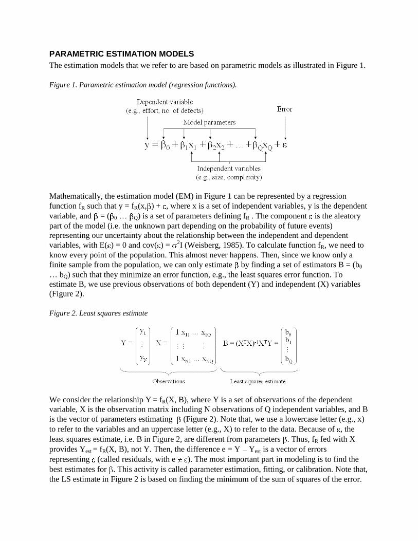
The estimation models that we refer to are based on parametric models as illustrated in Figure 1.

Figure 1. Parametric estimation model (regression functions).

Mathematically, the estimation model (EM) in Figure 1 can be represented by a regression

function fR such that y = fR(x, ) + , where x is a set of independent variables, y is the dependent

variable, and = ( 0 … Q) is a set of parameters defining fR . The component is the aleatory

part of the model (i.e. the unknown part depending on the probability of future events)

representing our uncertainty about the relationship between the independent and dependent

variables, with E( ) = 0 and cov( ) = 2I (Weisberg, 1985). To calculate function fR, we need to

know every point of the population. This almost never happens. Then, since we know only a

finite sample from the population, we can only estimate by finding a set of estimators B = (b0

… bQ) such that they minimize an error function, e.g., the least squares error function. To

estimate B, we use previous observations of both dependent (Y) and independent (X) variables

(Figure 2).

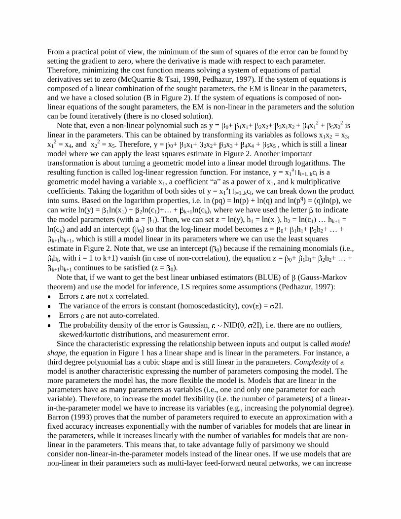
Figure 2. Least squares estimate

We consider the relationship Y = fR(X, B), where Y is a set of observations of the dependent

variable, X is the observation matrix including N observations of Q independent variables, and B

is the vector of parameters estimating (Figure 2). Note that, we use a lowercase letter (e.g., x)

to refer to the variables and an uppercase letter (e.g., X) to refer to the data. Because of , the

least squares estimate, i.e. B in Figure 2, are different from parameters . Thus, fR fed with X

provides Yest = fR(X, B), not Y. Then, the difference e = Y Yest is a vector of errors

representing (called residuals, with e ). The most important part in modeling is to find the

best estimates for . This activity is called parameter estimation, fitting, or calibration. Note that,

the LS estimate in Figure 2 is based on finding the minimum of the sum of squares of the error.

From a practical point of view, the minimum of the sum of squares of the error can be found by

setting the gradient to zero, where the derivative is made with respect to each parameter.

Therefore, minimizing the cost function means solving a system of equations of partial

derivatives set to zero (McQuarrie & Tsai, 1998, Pedhazur, 1997). If the system of equations is

composed of a linear combination of the sought parameters, the EM is linear in the parameters,

and we have a closed solution (B in Figure 2). If the system of equations is composed of non-

linear equations of the sought parameters, the EM is non-linear in the parameters and the solution

can be found iteratively (there is no closed solution).

Note that, even a non-linear polynomial such as y = 0+ 1x1+ 2x2+ 3x1x2 + 4x12 + 5x2

2 is

linear in the parameters. This can be obtained by transforming its variables as follows x1x2 = x3,

x12 = x4, and x2

2 = x5. Therefore, y = 0+ 1x1+ 2x2+ 3x3 + 4x4 + 5x5 , which is still a linear

model where we can apply the least squares estimate in Figure 2. Another important

transformation is about turning a geometric model into a linear model through logarithms. The

resulting function is called log-linear regression function. For instance, y = x1a

i=1..kci is a

geometric model having a variable x1, a coefficient “a” as a power of x1, and k multiplicative

coefficients. Taking the logarithm of both sides of y = x1a

i=1..kci, we can break down the product

into sums. Based on the logarithm properties, i.e. ln (pq) = ln(p) + ln(q) and ln(pq) = (q)ln(p), we

can write ln(y) = 1ln(x1) + 2ln(c1)+… + k+1ln(ck), where we have used the letter to indicate

the model parameters (with a = 1). Then, we can set z = ln(y), h1 = ln(x1), h2 = ln(c1) … hk+1 =

ln(ck) and add an intercept ( 0) so that the log-linear model becomes z = 0+ 1h1+ 2h2+ … +

k+1hk+1, which is still a model linear in its parameters where we can use the least squares

estimate in Figure 2. Note that, we use an intercept ( 0) because if the remaining monomials (i.e.,

ihi, with i = 1 to k+1) vanish (in case of non-correlation), the equation z = 0+ 1h1+ 2h2+ … +

k+1hk+1 continues to be satisfied (z = 0).

Note that, if we want to get the best linear unbiased estimators (BLUE) of (Gauss-Markov

theorem) and use the model for inference, LS requires some assumptions (Pedhazur, 1997):

Errors are not x correlated.

The variance of the errors is constant (homoscedasticity), cov( ) = 2I.

Errors are not auto-correlated.

The probability density of the error is Gaussian, NID(0, 2I), i.e. there are no outliers,

skewed/kurtotic distributions, and measurement error.

Since the characteristic expressing the relationship between inputs and output is called model

shape, the equation in Figure 1 has a linear shape and is linear in the parameters. For instance, a

third degree polynomial has a cubic shape and is still linear in the parameters. Complexity of a

model is another characteristic expressing the number of parameters composing the model. The

more parameters the model has, the more flexible the model is. Models that are linear in the

parameters have as many parameters as variables (i.e., one and only one parameter for each

variable). Therefore, to increase the model flexibility (i.e. the number of parameters) of a linear-

in-the-parameter model we have to increase its variables (e.g., increasing the polynomial degree).

Barron (1993) proves that the number of parameters required to execute an approximation with a

fixed accuracy increases exponentially with the number of variables for models that are linear in

the parameters, while it increases linearly with the number of variables for models that are non-

linear in the parameters. This means that, to take advantage fully of parsimony we should

consider non-linear-in-the-parameter models instead of the linear ones. If we use models that are

non-linear in their parameters such as multi-layer feed-forward neural networks, we can increase

the model flexibility (i.e. increasing the number of parameters) without adding new variables.

This is the real essence of the parsimony (Dreyfus, 2005, pp. 13-14).

However, as mentioned above, non-linear models do not have a closed solution for estimating

parameters B. Therefore, to overcome this problem, researchers and practitioners often prefer to

use models that are linear in the parameters instead of using the non-linear ones. However, if we

choose models that are linear in the parameters, finding the model shape that best fits the data is

much more difficult than if we used models that are non-linear in the parameters (Dreyfus, 2005,

pp. 136-138). Conversely, iterative procedures require a lot of experience to be effectively used

in practical problems. For instance, iterative procedures may provide different parameter

estimates depending on the initialization values (Bishop, 1995, pp. 140-148; Dreyfus, 2005, pp.

118-119). Therefore, finding the right parameters may require many attempts as well as the use

of optimization techniques to reduce the calibration time.

Estimation Model Accuracy

Prediction models may be evaluated in terms of Absolute Error (AE), i.e. AE = Actual –

Estimated = Y – Yest. However, an absolute error measure makes no sense when dealing with

estimation model accuracy for software engineering variables (e.g., effort, defects). In fact, an

Absolute Error would increase with the size of what we we’re predicting. Let AE1 (= 0.30) and

AE2 (= 0.25) be the absolute errors calculated by feeding the estimation model with data from

two different objects (e.g. project 1 and 2). Then, we might argue that the model is less accurate

for project 1 than for project 2 because AE1 expresses a lower accuracy than AE2 , i.e., AE1 >

AE2. However, if Y1 (the actual value from which AE1 has been calculated) were much greater

than Y2, i.e., Y1 >> Y2, and AE1 AE2 or even AE1 > AE2, then looking at the absolute error

AE1, we would incorrectly judge that the estimation model accuracy on object 1 is worse than

the accuracy on object 2. Actually, we should judge the accuracy on object 1 as better than the

accuracy on object 2, i.e. the (absolute) error should be evaluated with respect to the magnitude

of the predictions. For instance, it should be much more severe having a prediction error AE =

0.30 for a project of 100 man/months than a prediction error AE = 0.30 for a project of 10,000

man/months. This means that, an absolute measure should not be used for model comparison.

When predicting software engineering variables, the right choice is to consider a relative error

measure, i.e. a measure that takes into account the size of what we are predicting (Myrtveit,

Stensrud, & Shepperd, 2005). For this reason, Boehm (1981) defined the performance of his

software cost model (COnstructive COst MOdel, COCOMO) in terms of Relative Error (RE),

Eqn. 1.

RE = (Actual – Estimated)/Actual = (Y – Yest)/Y. (1)

Note that, currently the Boehm’s model has enhanced into the COCOMO-II (Boehm, Horowitz,

Madachy, Reifer, Clark, Steece, Brown, Chulani, & Abts, 2000), but the accuracy evaluation

principles have not changed. The evaluation procedure of the model accuracy is shown in Figure

3.

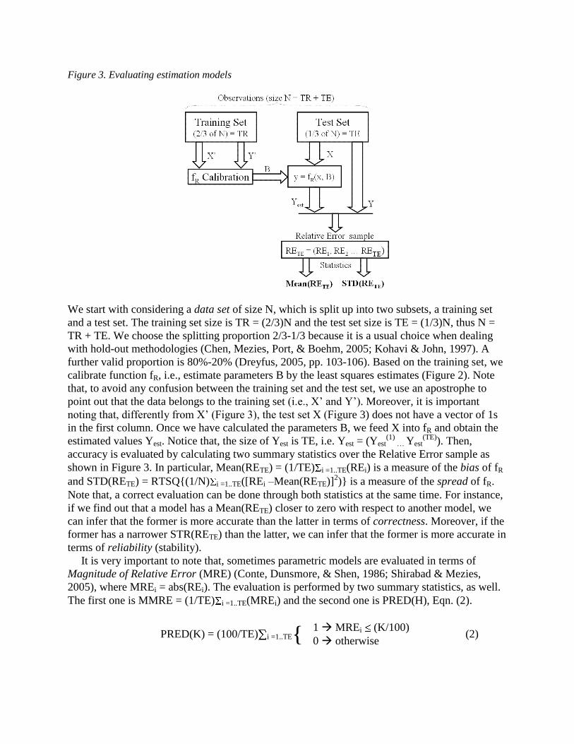
Figure 3. Evaluating estimation models

We start with considering a data set of size N, which is split up into two subsets, a training set

and a test set. The training set size is TR = (2/3)N and the test set size is TE = (1/3)N, thus N =

TR + TE. We choose the splitting proportion 2/3-1/3 because it is a usual choice when dealing

with hold-out methodologies (Chen, Mezies, Port, & Boehm, 2005; Kohavi & John, 1997). A

further valid proportion is 80%-20% (Dreyfus, 2005, pp. 103-106). Based on the training set, we

calibrate function fR, i.e., estimate parameters B by the least squares estimates (Figure 2). Note

that, to avoid any confusion between the training set and the test set, we use an apostrophe to

point out that the data belongs to the training set (i.e., X’ and Y’). Moreover, it is important

noting that, differently from X’ (Figure 3), the test set X (Figure 3) does not have a vector of 1s

in the first column. Once we have calculated the parameters B, we feed X into fR and obtain the

estimated values Yest. Notice that, the size of Yest is TE, i.e. Yest = (Yest(1)

… Yest(TE)). Then,

accuracy is evaluated by calculating two summary statistics over the Relative Error sample as

shown in Figure 3. In particular, Mean(RETE) = (1/TE) i =1..TE(REi) is a measure of the bias of fR

and STD(RETE) = RTSQ{(1/N) i =1..TE([REi –Mean(RETE)]2)} is a measure of the spread of fR.

Note that, a correct evaluation can be done through both statistics at the same time. For instance,

if we find out that a model has a Mean(RETE) closer to zero with respect to another model, we

can infer that the former is more accurate than the latter in terms of correctness. Moreover, if the

former has a narrower STR(RETE) than the latter, we can infer that the former is more accurate in

terms of reliability (stability).

It is very important to note that, sometimes parametric models are evaluated in terms of

Magnitude of Relative Error (MRE) (Conte, Dunsmore, & Shen, 1986; Shirabad & Mezies,

2005), where MREi = abs(REi). The evaluation is performed by two summary statistics, as well.

The first one is MMRE = (1/TE) i =1..TE(MREi) and the second one is PRED(H), Eqn. (2).

PRED(K) = (100/TE) i =1..TE{ 1 MREi (K/100)

(2) 0 otherwise

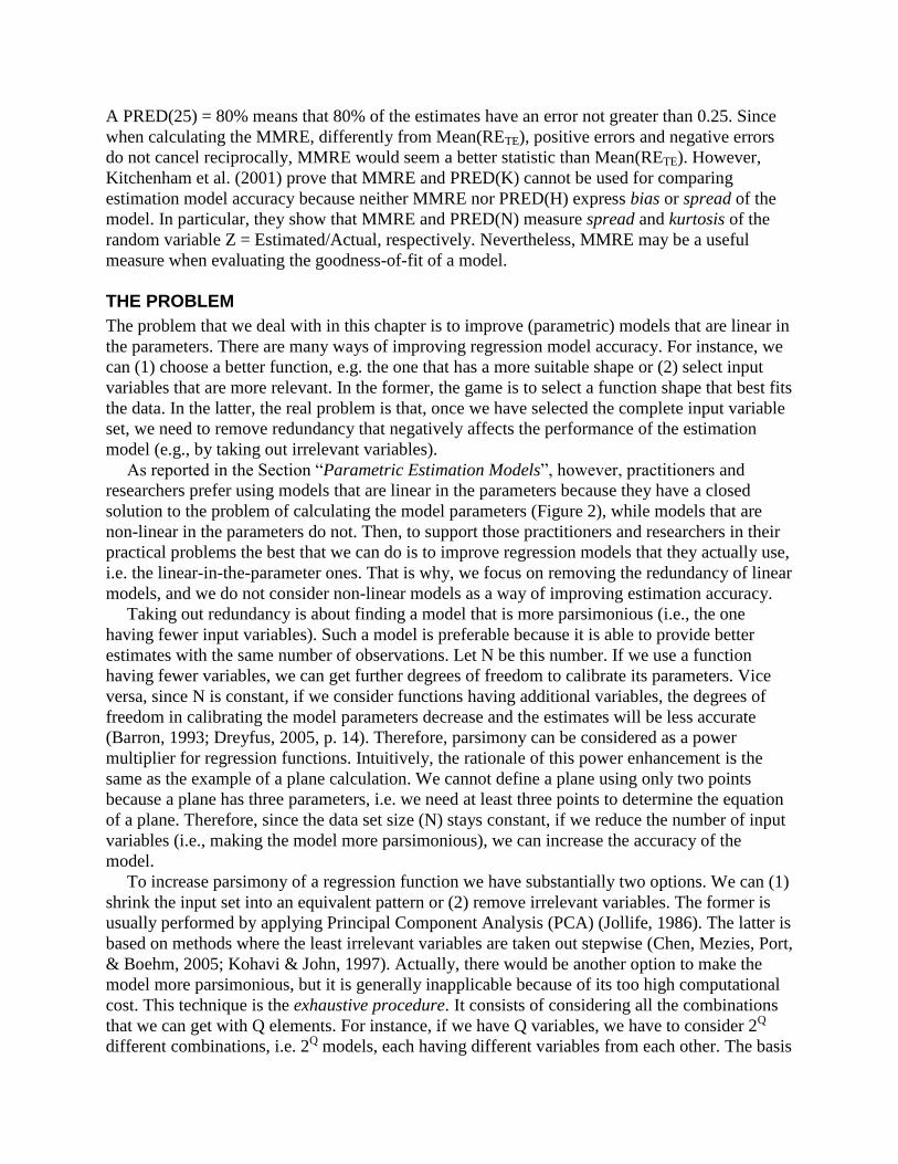
A PRED(25) = 80% means that 80% of the estimates have an error not greater than 0.25. Since

when calculating the MMRE, differently from Mean(RETE), positive errors and negative errors

do not cancel reciprocally, MMRE would seem a better statistic than Mean(RETE). However,

Kitchenham et al. (2001) prove that MMRE and PRED(K) cannot be used for comparing

estimation model accuracy because neither MMRE nor PRED(H) express bias or spread of the

model. In particular, they show that MMRE and PRED(N) measure spread and kurtosis of the

random variable Z = Estimated/Actual, respectively. Nevertheless, MMRE may be a useful

measure when evaluating the goodness-of-fit of a model.

THE PROBLEM

The problem that we deal with in this chapter is to improve (parametric) models that are linear in

the parameters. There are many ways of improving regression model accuracy. For instance, we

can (1) choose a better function, e.g. the one that has a more suitable shape or (2) select input

variables that are more relevant. In the former, the game is to select a function shape that best fits

the data. In the latter, the real problem is that, once we have selected the complete input variable

set, we need to remove redundancy that negatively affects the performance of the estimation

model (e.g., by taking out irrelevant variables).

As reported in the Section “Parametric Estimation Models”, however, practitioners and

researchers prefer using models that are linear in the parameters because they have a closed

solution to the problem of calculating the model parameters (Figure 2), while models that are

non-linear in the parameters do not. Then, to support those practitioners and researchers in their

practical problems the best that we can do is to improve regression models that they actually use,

i.e. the linear-in-the-parameter ones. That is why, we focus on removing the redundancy of linear

models, and we do not consider non-linear models as a way of improving estimation accuracy.

Taking out redundancy is about finding a model that is more parsimonious (i.e., the one

having fewer input variables). Such a model is preferable because it is able to provide better

estimates with the same number of observations. Let N be this number. If we use a function

having fewer variables, we can get further degrees of freedom to calibrate its parameters. Vice

versa, since N is constant, if we consider functions having additional variables, the degrees of

freedom in calibrating the model parameters decrease and the estimates will be less accurate

(Barron, 1993; Dreyfus, 2005, p. 14). Therefore, parsimony can be considered as a power

multiplier for regression functions. Intuitively, the rationale of this power enhancement is the

same as the example of a plane calculation. We cannot define a plane using only two points

because a plane has three parameters, i.e. we need at least three points to determine the equation

of a plane. Therefore, since the data set size (N) stays constant, if we reduce the number of input

variables (i.e., making the model more parsimonious), we can increase the accuracy of the

model.

To increase parsimony of a regression function we have substantially two options. We can (1)

shrink the input set into an equivalent pattern or (2) remove irrelevant variables. The former is

usually performed by applying Principal Component Analysis (PCA) (Jollife, 1986). The latter is

based on methods where the least irrelevant variables are taken out stepwise (Chen, Mezies, Port,

& Boehm, 2005; Kohavi & John, 1997). Actually, there would be another option to make the

model more parsimonious, but it is generally inapplicable because of its too high computational

cost. This technique is the exhaustive procedure. It consists of considering all the combinations

that we can get with Q elements. For instance, if we have Q variables, we have to consider 2Q

different combinations, i.e. 2Q models, each having different variables from each other. The basis

of the power is 2 because an element can belong to the set or not (binary choice). For each

model, the procedure goes on by calculating the error. Then, the model having the highest

accuracy is selected.

In this work, we present an empirical strategy to shrink the input set by applying an improved

version of PCA called Curvilinear Component Analysis (CCA) or non-linear Principal

Component Analysis (Sarcia’, Cantone, & Basili, 2008). We apply CCA instead of using PCA

because CCA is able to overcome some drawbacks affecting PCA. For instance, PCA can just

find linear redundancy, while CCA can find both linear and non-linear redundancy. Note that, to

increase the model parsimony we focus on input reduction techniques instead of the stepwise

ones because the former can be completely automated while the latter cannot. In fact, stepwise

techniques require making a decision as to variables to be removed, i.e. the least relevant

variables. If we do not know the relevance of each variable, stepwise techniques may be difficult

to be correctly applied.

CURVILINEAR COMPONENT ANALYSIS

CCA is a procedure for feature reduction that consists of turning a training set into a more

compact and equivalent representation. CCA is a compression technique that maps a set into

another set having fewer variables, where the mapping is non-linear. We implement CCA

through auto-associative multi-layer feed-forward neural networks (Bishop, 1995, pp. 314-319).

Implementing CCA does not require being an expert in neural network (NN). A CCA

implementation can be found in any mathematical application that is able to deal with NNs

and/or matrices. CCA requires just a few lines of code. Even if one does not have the opportunity

to use a mathematical suite, a CCA algorithm can be easily implemented through the same

programming language used for estimating the LS parameters. Before delving into details of

auto-associative neural networks, we provide some background on multi-layer feed-forward

neural networks.

Multi-layer Feed-forward Neural Networks

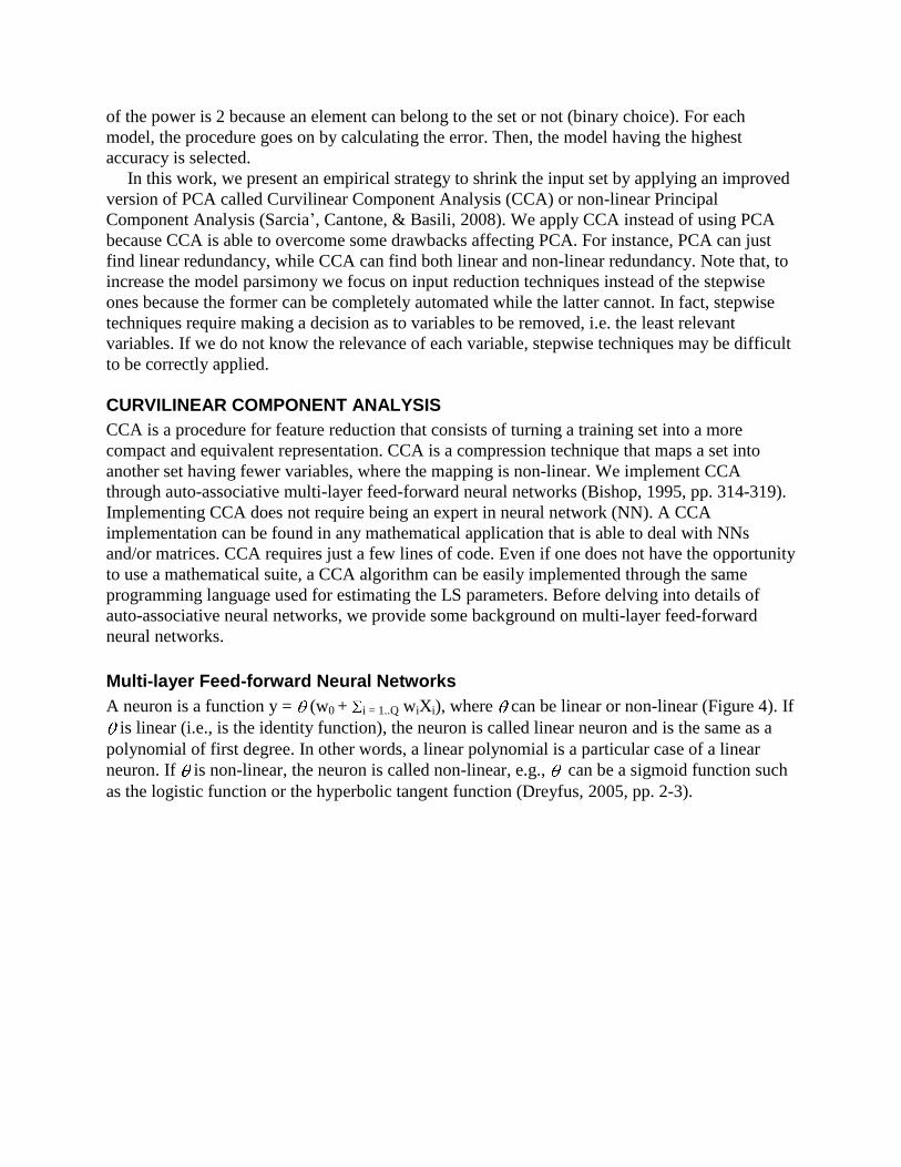
A neuron is a function y = (w0 + i = 1..Q wiXi), where can be linear or non-linear (Figure 4). If

is linear (i.e., is the identity function), the neuron is called linear neuron and is the same as a

polynomial of first degree. In other words, a linear polynomial is a particular case of a linear

neuron. If is non-linear, the neuron is called non-linear, e.g., can be a sigmoid function such

as the logistic function or the hyperbolic tangent function (Dreyfus, 2005, pp. 2-3).

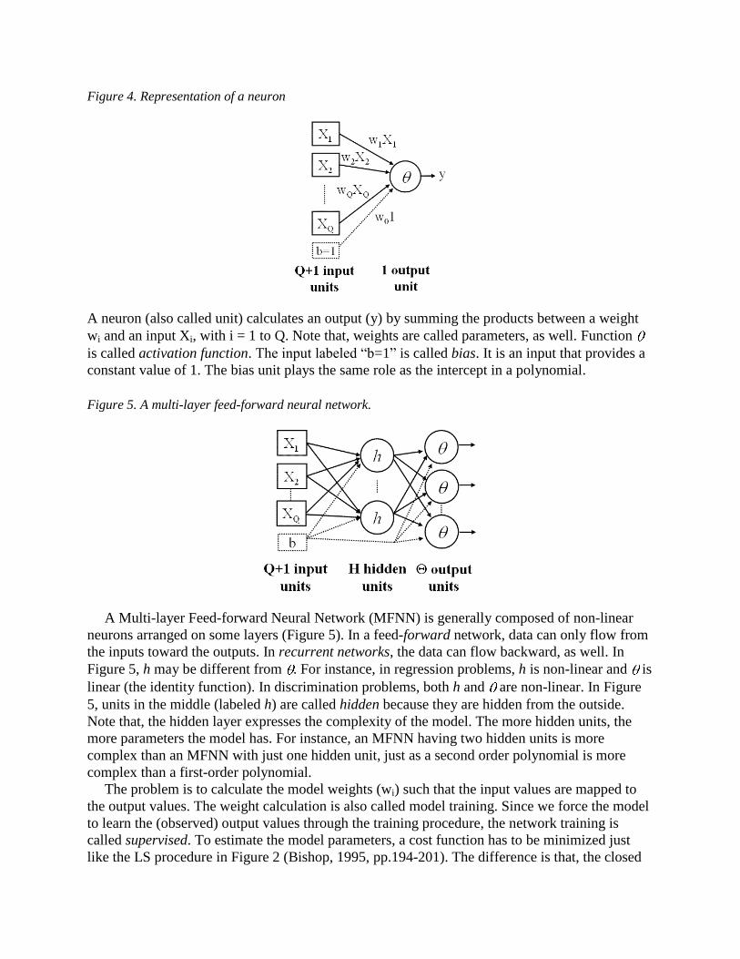
Figure 4. Representation of a neuron

A neuron (also called unit) calculates an output (y) by summing the products between a weight

wi and an input Xi, with i = 1 to Q. Note that, weights are called parameters, as well. Function

is called activation function. The input labeled “b=1” is called bias. It is an input that provides a

constant value of 1. The bias unit plays the same role as the intercept in a polynomial.

Figure 5. A multi-layer feed-forward neural network.

A Multi-layer Feed-forward Neural Network (MFNN) is generally composed of non-linear

neurons arranged on some layers (Figure 5). In a feed-forward network, data can only flow from

the inputs toward the outputs. In recurrent networks, the data can flow backward, as well. In

Figure 5, h may be different from . For instance, in regression problems, h is non-linear and is

linear (the identity function). In discrimination problems, both h and are non-linear. In Figure

5, units in the middle (labeled h) are called hidden because they are hidden from the outside.

Note that, the hidden layer expresses the complexity of the model. The more hidden units, the

more parameters the model has. For instance, an MFNN having two hidden units is more

complex than an MFNN with just one hidden unit, just as a second order polynomial is more

complex than a first-order polynomial.

The problem is to calculate the model weights (wi) such that the input values are mapped to

the output values. The weight calculation is also called model training. Since we force the model

to learn the (observed) output values through the training procedure, the network training is

called supervised. To estimate the model parameters, a cost function has to be minimized just

like the LS procedure in Figure 2 (Bishop, 1995, pp.194-201). The difference is that, the closed

solution of B in Figure 2 does not apply to MFNNs. We have to estimate the model parameters

iteratively. The most effective iterative training technique is the Backpropagation (Rumelhart,

Hilton, & Williams, 1986). This is a method based on calculating the gradient of the cost

function step-by-step. For each step, the gradient is used to update the parameters found in the

previous step. The algorithm stops when satisfactory conditions have been met. It is important to

note that, the hidden neurons play a primary role here. In fact, their output can be considered as a

representation of the input in mapping the output (Rumelhart, Hilton, & Williams, 1986). This

property will be used for implementing Auto-Associative Neural Networks.

Auto-associative Multi-layer Feed-forward Neural Networks

An Auto-Associative Neural Network (AANN) is a particular kind of MFNN. Figure 6 shows an

example of its topology.

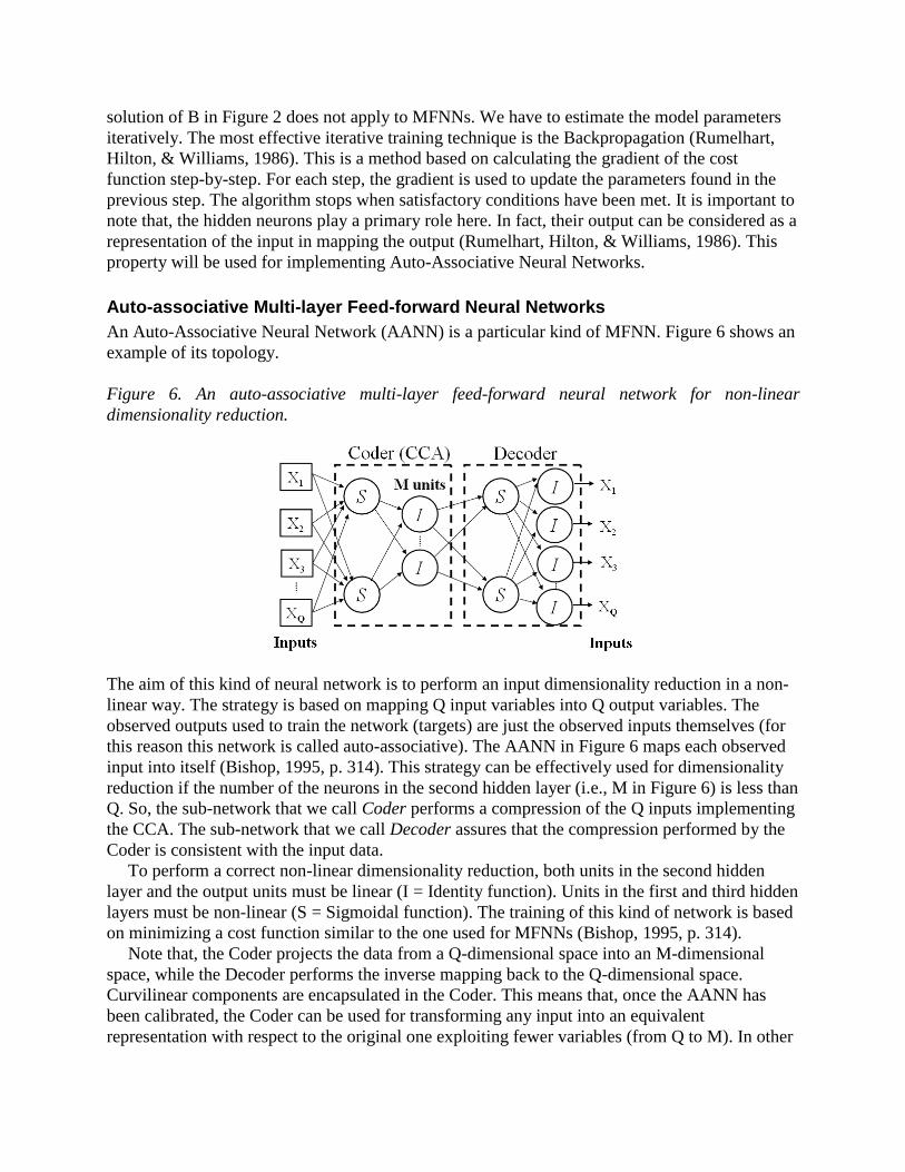
Figure 6. An auto-associative multi-layer feed-forward neural network for non-linear

dimensionality reduction.

The aim of this kind of neural network is to perform an input dimensionality reduction in a non-

linear way. The strategy is based on mapping Q input variables into Q output variables. The

observed outputs used to train the network (targets) are just the observed inputs themselves (for

this reason this network is called auto-associative). The AANN in Figure 6 maps each observed

input into itself (Bishop, 1995, p. 314). This strategy can be effectively used for dimensionality

reduction if the number of the neurons in the second hidden layer (i.e., M in Figure 6) is less than

Q. So, the sub-network that we call Coder performs a compression of the Q inputs implementing

the CCA. The sub-network that we call Decoder assures that the compression performed by the

Coder is consistent with the input data.

To perform a correct non-linear dimensionality reduction, both units in the second hidden

layer and the output units must be linear (I = Identity function). Units in the first and third hidden

layers must be non-linear (S = Sigmoidal function). The training of this kind of network is based

on minimizing a cost function similar to the one used for MFNNs (Bishop, 1995, p. 314).

Note that, the Coder projects the data from a Q-dimensional space into an M-dimensional

space, while the Decoder performs the inverse mapping back to the Q-dimensional space.

Curvilinear components are encapsulated in the Coder. This means that, once the AANN has

been calibrated, the Coder can be used for transforming any input into an equivalent

representation with respect to the original one exploiting fewer variables (from Q to M). In other

words, the Coder can execute a non-linear dimensionality reduction (CCA). This important result

is made possible because of the presence of non-linear functions in the first and third hidden

layer (S). This kind of AANN is able to perform also a linear dimensionality reduction as a

particular case of the non-linear one.

THE EMPIRICAL STRATEGY FOR MODEL IMPROVEMENT

The aim of the model improvement strategy is to find empirically the most accurate model.

Consider two distinct models EM1 and EM2 being compared. As discussed in the Section

“Estimation Model Accuracy”, we can argue that EM1 is more accurate (correct) than EM2 if two

conditions are satisfied at the same time: (1) the bias of EM1 is closer to zero than the bias of

EM2 and (2) the spread of EM1 is not worse than the spread of EM2. The problem is that, CCA

can be applied with different reduction rates, i.e. with respect to Figure 6, the number of the units

in the second hidden layer (M) may be set to M = Q through to 1, where M = Q means no

reduction and M = 1 means that the shrunken input data is expressed by only one component.

But, we do not know the best CCA reduction rate (M), i.e. the one that bears the most accurate

estimation model. To find it, we use an empirical strategy reported below (Sarcia’, Cantone, &

Basili, 2008). The authors show that the strategy together with CCA can significantly improve

accuracy of log-linear regression models calibrated on the COCOMO 81 data set (Shirabad &

Menzies, 2005). The strategy is the following:

Precondition

Rely on a data set (DS) of past observations where each of them is expressed by Q

independent variables x1, x2 … xQ and the DS size is N (i.e. DSQXN) with N (= TR + TE)

statistically significant

Independent variables x1, x2 … xQ are relevant to predict the dependent variable y and

constitute the complete input set (Dreyfus, 2005, pp. 95-96).

Procedure

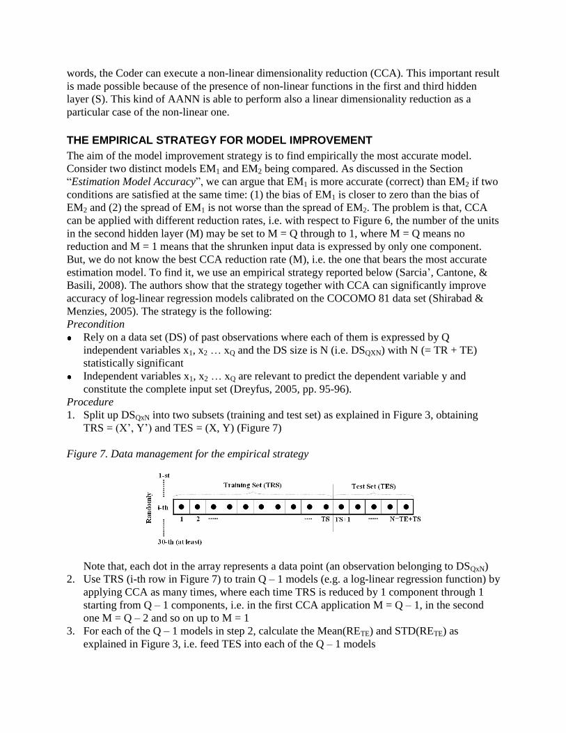
1. Split up DSQxN into two subsets (training and test set) as explained in Figure 3, obtaining

TRS = (X’, Y’) and TES = (X, Y) (Figure 7)

Figure 7. Data management for the empirical strategy

Note that, each dot in the array represents a data point (an observation belonging to DSQxN)

2. Use TRS (i-th row in Figure 7) to train Q – 1 models (e.g. a log-linear regression function) by

applying CCA as many times, where each time TRS is reduced by 1 component through 1

starting from Q – 1 components, i.e. in the first CCA application M = Q – 1, in the second

one M = Q – 2 and so on up to M = 1

3. For each of the Q – 1 models in step 2, calculate the Mean(RETE) and STD(RETE) as

explained in Figure 3, i.e. feed TES into each of the Q – 1 models

4. Based on the Q – 1 models obtained in step 2, select the model having the best Mean(RETE)

i.e., the closest to zero

5. Use TRS to train a model without applying CCA (labeled NO-CCA hereafter), i.e. a model

without reduction

6. Calculate the Mean(RETE) and STD(RETE) feeding TES into the NO-CCA model (step 5)

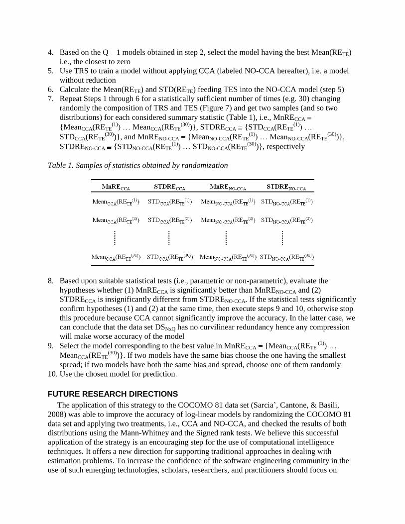
7. Repeat Steps 1 through 6 for a statistically sufficient number of times (e.g. 30) changing

randomly the composition of TRS and TES (Figure 7) and get two samples (and so two

distributions) for each considered summary statistic (Table 1), i.e., MnRECCA

{MeanCCA(RETE(1)) … MeanCCA(RETE

(30))}, STDRECCA {STDCCA(RETE(1)) …

STDCCA(RETE(30))}, and MnRENO-CCA {MeanNO-CCA(RETE

(1)) … MeanNO-CCA(RETE(30))},

STDRENO-CCA {STDNO-CCA(RETE(1)) … STDNO-CCA(RETE

(30))}, respectively

Table 1. Samples of statistics obtained by randomization

8. Based upon suitable statistical tests (i.e., parametric or non-parametric), evaluate the

hypotheses whether (1) MnRECCA is significantly better than MnRENO-CCA and (2)

STDRECCA is insignificantly different from STDRENO-CCA. If the statistical tests significantly

confirm hypotheses (1) and (2) at the same time, then execute steps 9 and 10, otherwise stop

this procedure because CCA cannot significantly improve the accuracy. In the latter case, we

can conclude that the data set DSNxQ has no curvilinear redundancy hence any compression

will make worse accuracy of the model

9. Select the model corresponding to the best value in MnRECCA {MeanCCA(RETE (1)) …

MeanCCA(RETE(30))}. If two models have the same bias choose the one having the smallest

spread; if two models have both the same bias and spread, choose one of them randomly

10. Use the chosen model for prediction.

FUTURE RESEARCH DIRECTIONS

The application of this strategy to the COCOMO 81 data set (Sarcia’, Cantone, & Basili,

2008) was able to improve the accuracy of log-linear models by randomizing the COCOMO 81

data set and applying two treatments, i.e., CCA and NO-CCA, and checked the results of both

distributions using the Mann-Whitney and the Signed rank tests. We believe this successful

application of the strategy is an encouraging step for the use of computational intelligence

techniques. It offers a new direction for supporting traditional approaches in dealing with

estimation problems. To increase the confidence of the software engineering community in the

use of such emerging technologies, scholars, researchers, and practitioners should focus on

replicating past experiments and performing new investigations based on different settings, e.g.,

by changing contexts and variables of interest.

An important future area of research is to compare the proposed CCA strategy to stepwise

feature selection techniques, as well as exploring the possibility of defining a new strategy that

combines both techniques.

CONCLUSION

In this chapter, we have discussed some issues concerning parametric estimation models based

on regression functions. We have shown that these functions are relevant for any kind of

estimation methodology even for human-based judgment techniques (McConnell, 2006, pp. 105-

112). The problem of improving the performance of regression functions is a major issue for any

software organization that aims at delivering their products on time, on budget, and with the

required quality. To improve the performance of regression functions, we have presented an

empirical strategy based on a shrinking technology called CCA and showed its implementation

by auto-associative neural networks. We have discussed the reasons why CCA is able to increase

accuracy (correctness) without worsening the spread (variability) of the model (Sarcia’, Cantone,

& Basili, 2008). We have focused on the possibility of CCA to make models more parsimonious.

Let us now consider the implications of the empirical strategy reported above. From a

practical point of view, an advantage of applying CCA is that we do not need to know the

relevance of each attribute being removed with respect to the considered context. This is an

advantage because, if we do not know the relevance of the attributes being removed, as stepwise

feature selection techniques do, we cannot improve the model making it more parsimonious

(Chen, Mezies, Port, & Boehm, 2005; Kohavi & John, 1997). Moreover, CCA does not suffer

from multicollinearity, which affects stepwise methods. Multicollinearity is a statistical effect

based on the impossibility of separating the influence of two or more input variables on the

output (Weisberg, 1985). CCA overcomes this problem by considering the simultaneous effect of

every input variable by finding non-linear redundancy of input variables in predicting the output.

A further advantage is that, CCA can be completely automated, i.e. it does not require any

human interaction to be carried out.

A real application of the presented strategy, is reported in (Sarcia’, Cantone, & Basili, 2008),

where the authors provide some suggestions as to experimental setting, data management, and

statistical tests. The authors find that, with respect to the COCOMO 81 data set, the proposed

strategy increases correctness without worsening the reliability of log-linear regression models.

Note that, the authors not only compared the medians, but also the standard deviations of the two

distributions (i.e., CCA and NO-CCA). As presented above, they applied two non-parametric

tests (Mann-Whitney and Signed rank) because a preliminary normality test on both distributions

showed that the distributions could not be considered as coming from a normal population.

Further results were that, applying the proposed strategy reduces the occurrence of outliers. In

other words, estimates obtained by models treated with CCA show fewer outliers than models

treated without applying CCA. This means that, CCA can improve reliability in terms of outlier

reduction even though correctness may not be improved. This is a valuable result for researchers

and practitioners because they may just use the strategy to build models less prone to outliers.

The strategy has some drawbacks. For instance, it has been built on the assumption of having

enough data to split up the data set into two subsets (TRS and TES). Conversely, if we do not

have enough data, CCA would not be applicable. CCA is based on building specific multi-layer

neural networks, which require some optimization techniques to reduce the training time (Hagan

& Menhaj, 1994).

REFERENCES

Barron, A. (1993). Universal approximation bounds for superposition of a sigmoidal function.

IEEE Transaction on Information Theory, 39(1), 930-945.

Boehm, B. (1981). Software Engineering Economics. Upper Saddle River, New Jersey, USA:

Prentice-Hall.

Boehm, B., Horowitz, E., Madachy, R., Reifer, D., Clark, B.K., Steece, B., Brown, A.W.,

Chulani, S., & Abts, C. (2000). Software Cost Estimation with COCOMO II. Upper Saddle

River, New Jersey, USA: Prentice-Hall.

Bishop, C. (1995). Neural Network for Pattern Recognition. New York, NY, USA: Oxford

University Press.

Chen, Z. Mezies, T. Port, D., & Boehm, B.W. (2005). Feature Subset Selection Can Improve

Software Cost Estimation Accuracy. In T. Mezies (Ed.), PROMISE ’05 (pp. 1-6). ACM.

Conte, S.D., Dunsmore, H.E., & Shen, V.Y. (1986). Software Engineering Metrics and Models.

Menlo Park, CA, USA: The Benjamin/Cummings Publishing Company, Inc.

Dreyfus, G. (2005). Neural Networks Methodology and Applications. Berlin, Germany:

Springer.

Hagan, M.T., & Menhaj, M.B. (1994). Training Feedforward Networks with the Marquardt

Algorithm. IEEE Transactions on Neural Networks. 5(6), 989-993.

Jollife, I.T. (1986). Principal Component Analysis. Berlin, Germany: Springer.

Kitchenham, B., MacDonell, S., Pickard, L., & Shepperd, M. (2001). What accuracy statistics

really measure. IEE Proceedings: Vol. 148. Software Engineering (pp. 81-85). IEE Proceeding.

Kohavi, R., & John, G.H. (1997). Wrappers for feature subset selection. ACM Artificial

Intelligence, 97(1-2), 273-324.

McConnell, S. (2006). Software Estimation – Demystifying the Black Art. Redmond, WA, USA:

Microsoft press.

McQuarrie, A.D.R., & Tsai, C. (1998). Regression and Time Series Model Selection. Singapore:

World Scientific Publishing Co. Pte. Ltd..

Myrtveit, I., Stensrud, E., & Shepperd, M. (2005). Reliability and Validity in Comparative

Studies of Software Prediction Models. IEEE Transaction on Software Engineering, 31(5), 380-

391.

Pedhazur, E.J. (1997). Multiple Regression in Behavioral Research. Orlando, FL, USA: Harcourt

Brace.

Rumelhart, D.E., Hilton, G.E., & Williams, R.J. (1986). Learning Internal Representations by

Error Propagation. In D. Rumelhart & J. McClelland (Ed.): Parallel Distributing Computing:

Explorations in the Microstructure of Cognition: Vol. 1. (pp. 318-362). The MIT press.

Sarcia’, S.A., Cantone, G, & Basili, V.R (2008). Adopting Curvilinear Component Analysis to

Improve Software Cost Estimation Accuracy. Model, Application Strategy, and an Experimental

Verification. In G. Visaggio (Ed.), 12th

International Conference on Evaluation and Assessment

in Software Engineering. BCS eWIC.

Shepperd, M. (2007). Software project economics: a roadmap. International Conference on

Software Engineering 2007: Vol. 1. IEEE Future of Software Engineering (pp. 304-315). IEEE

Computer Society

Shirabad, J.S., & Menzies, T. (2005). The PROMISE Repository of Software Engineering

Databases. School of Information Technology and Engineering of the University of Ottawa,

Canada. Retrieved August 31, 2008, from http://promise.site.uottawa.ca/SERepository.

Weisberg, S. (1985). Applied Linear Regression, New York, NY, USA: John Wiley and Sons.

ADDITIONAL READING

Aha, D.W., & Bankert, R.L. (1996). A comparative evaluation of sequential feature selection

algorithms. Artificial Intelligence and Statistics. New York, NY, USA: Springer-Verlag.

Angelis, L., & Stamelos, I. (2000). A Simulation Tool for efficient analogy based cost

estimation,” Empirical Software Engineering, 5(1), 35-68.

Basili, V.R., & Weiss, D. (1984). A Methodology for Collecting Valid Software Engineering

Data. IEEE Transactions on Software Engineering, 3(1), 728-738.

Bishop, C., & Qazaz, C.S. (1995). Bayesian inference of noise levels in regression. International

Conference on Artificial Neural Networks: Vol. 2. EC2 & Cie (pp. 59-64). ICANN95.

Briand, L.C., Basili, V.R. & Thomas, W. (1992). A pattern recognition approach to software

engineering data analysis. IEEE Transactions on Software Engineering. 18(11), 931-942, IEEE

Computer Society.

Briand, L.C., El-Emam, K., Maxwell, K., Surmann, D., & Wieczorek, I. (1999). An Assessment

and Comparison of Common Cost Software Project Estimation Methods. Proceeding of the 1999

International Conference on Software Engineering (pp. 313-322): IEEE Computer Society.

Briand, L.C., Langley, T., & Wieczorek, I. (2000). A Replicated Assessment and Comparison of

Common Software Cost Modeling Techniques. Proceeding of the 2000 International Conference

on Software Engineering (pp. 377-386). IEEE Computer Society.

Cantone, G., & Donzelli, P. (2000). Production and Maintenance of Goal-oriented Measurement

Models. World Scientific, 105(4), 605-626.

Fenton, N. E. (1991). Software Metrics: A Rigorous Approach. London, UK: Chapman & Hall.

Finnie, G., Wittig, G., & Desharnais, J.-M. (1997). A comparison of software effort estimation

techniques using function points with neural networks, case based reasoning and regression

models. Journal of Systems & Software. 39(3), 281-289.

Foss, T., Stensrud, E., Kitchenham, B., & Myrtveit, I. (2003). A Simulation Study of the Model

Evaluation Criterion MMRE. IEEE Transaction on Software Eng. 29(11), 985-995.

Gulezian, R. (1991). Reformulating and calibrating COCOMO. Journal of Systems & Software.

16(6), 235-242.

Guyon, I, Gunn, M., Nikravesh, & Zadeh, L. (2005). Feature Extraction foundations and

applications. Berlin, Germany: Springer.

Jeffery, R., & Low, G. (1990). Calibrating estimation tools for software development. Software

Engineering Journal. 5(4), 215-221.

John, G., Kohavi, R., & Pfleger, K. (1994). Irrelevant features and the subset selection problem.

11th Intl. Conference on Machine Learning (pp. 121-129). Morgan Kaufmann.

Kemerer, C.F., (1987). An Empirical Validation of Software Cost Estimation Models. ACM

Communications, 30(5), 416-429.

Khoshgoftaar, T. M., & Lanning, D. L. (1995). A Neural Network Approach for Early Detection

of Program Modules Having High Risk in the Maintenance Phase. Journal of Systems Software.

29(1), 85-91.

Khoshgoftaar, T. M., Lanning, D. L., & Pandya, A. S. (1994). A comparative-study of pattern-

recognition techniques for quality evaluation of telecommunications software. IEEE Journal on

Selected Areas In Communications, 12(2), 279-291.

Kirsopp, C. & Shepperd, M. (2002). Case and Feature Subset Selection in Case-Based Software

Project Effort Prediction. Research and Development in Intelligent Systems XIX, New York, NY,

USA: Springer-Verlag.

Menzies, T., Port, D., Chen, Z., & Hihn, J. (2005). Validation Methods for Calibrating Software

Effort Models. Proceeding of the 2000 International Conference on Software Engineering (587-

595). IEEE Computer Society.

Myrtveit, I., & Stensrud, E. (1999). A controlled experiment to assess the benefits of estimating

with analogy and regression models. IEEE Transaction on Software Engineering, 25(4), 510-

525.

Myrtveit, I., & Stensrud, E. (2004). Do Arbitrary Function Approximators make sense as

Software Prediction Models? 12-th International Workshop on Software Technology and

Engineering Practice (pp. 3-9). IEEE Computer Society.

Neumann, D.E. (2002). An Enhanced Neural Network Technique for Software Risk Analysis.

IEEE Transaction on Software Engineering, 28(9), 904-912.

Rao, C.R. (1973). Linear Statistical Inference and its Applications. New York, NY, USA: Wiley

& Sons.

Srinivasan, K., & Fisher, D. (1995). Machine Learning Approaches to Estimating Software

Development Effort. IEEE Transaction on Software Engineering, 21(2), 126-137.

Stensrud, E., Foss, T., Kitchenham, B., & Myrtveit, I. (2002). An empirical Validation of the

Relationship between the Magnitude of Relative Error and Project Size. Proceeding of the 8-th

IEEE Symposium on Software Metrics (pp. 3-12). IEEE Computer Society.

Vapnik, V.N. (1995). The Nature of Statistical Learning Theory. New York, NY, USA:

Springer-Verlag.

Wohlin, C., Runeson, P., Höst, M., Ohlsson, M.C., Regnell, B., & Wesslén, A. (2000).

Experimentation in Software Engineering – An Introduction. Berlin, Germany: Springer.

Salvatore Alessandro Sarcia' received his laurea degree in Computer Science (1994) and

master degree with honors in Strategy and Project Management (2001) from the University of

Torino (Italy). He received his second laurea degree in Politics (2004) from the University of

Trieste (Italy). In December 2008, he received his Ph.D. degree in Informatics and Automation

Engineering from the University of Rome “Tor Vergata” (Italy). In 2006-08, he was with the

Department of Computer Science of the University of Maryland (College Park, MD, USA) as a

Faculty Research Assistant. Mr. Sarcia’ is an untenured Professor of Object-Oriented

Programming at the DISP - University of Rome “Tor Vergata”. His research interests lay in the

area of Computational Intelligence (Artificial Neural Networks), Predictive Models, and

Statistics. He applies empirical techniques to conduct experiments on Software Engineering,

Software Quality, and Risk Analysis.

Dr. Salvatore Alessandro Sarcia’

DISP - University of Rome “Tor Vergata”

Via del Politecnico, 1

00133 Rome (Italy)

Voice: +39.06.7259.7942, Fax: +39.06.7259.7460

http://www.onese.org/sarcia

sarcia@disp.uniroma2.it

Victor R. Basili is Professor Emeritus at the University of Maryland. He

holds a PH.D. in Computer Science from the University of Texas and two honorary degrees. He

was Director of the Fraunhofer Center - Maryland and a director of the Software Engineering

Laboratory at NASA/GSFC. He has worked on measuring, evaluating, and improving the

software development process and product for over 35 years with numerous companies and

government agencies. Methods include Iterative Enhancement, the Goal Question Metric

Approach (GQM), the Quality Improvement paradigm (QIP), and the Experience Factory (EF).

Dr. Basili has authored over 250 peer reviewed publications and is a recipient of several awards

including the NASA Group Achievement Awards, ACM SIGSOFT Outstanding Research

Award, IEEE Computer Society Harlan Mills Award, and the Fraunhofer Medal. He is Co-EIC

of the Springer Empirical software Engineering Journal and an IEEE and ACM Fellow.

Professor Victor Robert Basili

Department of Computer Science and Institute for Advanced Computer Studies

University of Maryland

College Park, Maryland 20742

Phone: 301-405-2668 Fax: 301-405-3691

http://www.cs.umd.edu/~basili/

basili@cs.umd.edu

and

Fraunhofer Center for Experimental Software Engineering - Maryland

College Park Maryland 20742

Phone: 301-403-8934 Fax:301-403-8976

http://fc-md.umd.edu

Professor Giovanni Cantone is Professor at the University of Rome “Tor Vergata” teaching

Software Analysis, Design, and Architectures.

Professor Giovanni Cantone

DISP - University of Rome “Tor Vergata”

Via del Politecnico, 1

00133 Rome (Italy)

Voice: +39.06.7259.7392, Fax: +39.06.7259.7460

cantone@uniroma2.it