Atmospheric Chemistry and Physics - HKU Scholars Hub

Atmos. Chem. Phys., 10, 4013–4031, 2010www.atmos-chem-phys.net/10/4013/2010/doi:10.5194/acp-10-4013-2010© Author(s) 2010. CC Attribution 3.0 License.

AtmosphericChemistry

and Physics

Corrigendum to

“A novel downscaling technique for the linkage of global andregional air quality modeling” published in Atmos. Chem. Phys.,9, 9169–9185, 2009

Y. F. Lam and J. S. Fu

Department of Civil and Environmental Engineering, University of Tennessee, Knoxville, TN, USA

We have discovered that the previously published paper wasnot the latest version of the manuscript we intended to use.Some corrections made during the second ACPD reviewingprocess were not incorporated in the text. As a result, thefigure numbers (i.e., figure number below the graph) werenot referenced correctly in the manuscript. Therefore, wehave decided to re-publish this paper as a corrigendum.

Abstract. Recently, downscaling global atmospheric modeloutputs (GCTM) for the USEPA Community Multiscale AirQuality (CMAQ) Initial (IC) and Boundary Conditions (BC)have become practical because of the rapid growth of com-putational technologies that allow global simulations to becompleted within a reasonable time. The traditional methodof generating IC/BC by profile data has lost its advocatesdue to the weakness of the limited horizontal and verticalvariations found on the gridded boundary layers. Theoret-ically, high quality GCTM IC/BC should yield a better re-sult in CMAQ. Unfortunately, several researchers have foundthat the outputs from GCTM IC/BC are not necessarily betterthan profile IC/BC due to the excessive transport of O3 aloftin GCTM IC/BC. In this paper, we intend to investigate theeffects of using profile IC/BC and global atmospheric modeldata. In addition, we are suggesting a novel approach to re-solve the existing issue in downscaling.

In the study, we utilized the GEOS-Chem model out-puts to generate time-varied and layer-varied IC/BC foryear 2002 with the implementation of tropopause determin-ing algorithm in the downscaling process (i.e., based onchemical (O3) tropopause definition). The comparison be-

Correspondence to:J. S. Fu([email protected])

tween the implemented tropopause approach and the profileIC/BC approach is performed to demonstrate improvementof considering tropopause. It is observed that without us-ing tropopause information in the downscaling process, un-realistic O3 concentrations are created at the upper layers ofIC/BC. This phenomenon has caused over-prediction of sur-face O3 in CMAQ. In addition, the amount of over-predictionis greatly affected by temperature and latitudinal locationof the study domain. With the implementation of the al-gorithm, we have successfully resolved the incompatibilityissues in the vertical layer structure between global and re-gional chemistry models to yield better surface O3 predic-tions than profile IC/BC for both summer and winter condi-tions. At the same time, it improved the vertical O3 distri-bution of CMAQ outputs. It is strongly recommended thatthe tropopause information should be incorporated into anytwo-way coupled global and regional models, where the tro-pospheric regional model is used, to solve the vertical incom-patibility that exists between global and regional models.

1 Introduction

Regional air quality models are designed to simulate thetransport, production, and destruction of atmospheric chem-icals at the tropospheric level. Particular interest is givenat the planetary boundary layer (PBL) where human activ-ities reside (Byun and Schere, 2006). Performance of theregional models depends greatly on the temporal and spa-tial quality of the inputs (i.e., emission inventories, meteoro-logical model outputs, and boundary conditions). Recently,establishing proper boundary conditions (BCs) has becomea crucial process as the effects of intercontinental transportof air pollutants (Heald et al., 2003; Lin et al., 2008; Chin

Published by Copernicus Publications on behalf of the European Geosciences Union.

http://creativecommons.org/licenses/by/3.0/

4014 Y. F. Lam and J. S. Fu: Corrigendum

et al., 2007) and enhancement of background pollutant con-centrations emerged (Vingarzan, 2004; Ordonez et al., 2007;Fiore et al., 2003). Various studies suggested that utilizingdynamic global chemical transport model (CTM) outputs asthe BCs for the regional air quality model would be the bestoption for capturing the temporal variation and spatial distri-butions of the tracer species (Fu et al., 2008; Byun et al.,2004; Morris et al., 2006; Tang et al., 2007). For exam-ple, Song et al., (2008) applied the interpolated values froma global chemical model, RAQMS, as the lateral BCs for theregional air quality model, CMAQ and evaluated simulatedCMAQ results with ozone soundings. Simulations were per-formed on the standard CMAQ seasonal varied profile BCsand dynamic BCs from RAQMS. The results demonstratedthat the scenario with dynamic BCs performed better thanthe scenario with profile BCs in terms of the prediction ofvertical ozone profile.

The quality of BCs depends on the vertical, horizontal, andtemporal resolutions of global CTM outputs. The latitudi-nal location and seasonal variation are also playing an im-portant role, which defines the tropopause height that influ-ences the vertical interpolation process between global andregional models. (Bethan et al., 1996; Stohl et al., 2003) Inthe MICS-Asia project, high concentrations of ozone (i.e.,500 ppbv) have been observed in CMAQ BCs when the re-gional model’s layers reach above or beyond the tropopauseheight during the vertical interpolation process. (Fu et al.,2008) This high ozone aloft in BCs has created problemsfor the regional tropospheric model (such as CMAQ) sinceit does not have a stratospheric component or stratosphere-troposphere exchange mechanism. As a result, unrealisti-cally high ozone concentrations were observed at the sur-face layer during the regional CTM simulations. Tang etal. (2009) studied various CTM lateral BCs from MOZART-NCAR, MOZART-GFDL, and RAQMS. They observed thatCTM BCs have induced a high concentration of ozone in theupper troposphere in CMAQ; this high ozone aloft quicklymixed down to the surface resulting in an overestimation ofsurface ozone. Mathur et al., suggested that the overesti-mation of O3 might also be partially contributed by the in-adequate representation of free tropospheric mixing due tothe selection of a coarse vertical resolution (Mathur et al.,2008; Tang et al., 2009) Since the rate of vertical trans-port of flux is highly sensitive to temperature and moisture-induced buoyancies, correctly representing deep convectionor flux entrainment at the unstable layer in the meteorologicalmodel becomes critical to modeling ozone vertical mixing. Itshould be noted that the single PBL scheme in the meteoro-logical model is not sufficient to simulate the correct verticallayer structure on the broad aspect of environmental condi-tions (i.e., terrain elevation and PBL height) in the existingdomain. As a result, it introduces uncertainties and errorsto the process of determining vertical transport of O3 in theair quality model (Zangl et al., 2008; Perez et al., 2006) Forthe downscaling problem, Tang et al. (2009) has commented

that using outputs of the global CTM (GCTM) as BCs maynot necessarily be better than the standard profile-BC, whichhighly depends on location and time. The quick downwardmixing in CMAQ has caused an erroneous prediction of sur-face ozone when both tropospheric and stratospheric ozoneare included in the CTM BCs. (Al-Saadi et al., 2007; Tanget al., 2007; Tang et al., 2009) Therefore, correctly defin-ing tropopause height for separating troposphere and strato-sphere becomes crucial to the prevention of stratospheric in-fluence during the vertical interpolation process for CMAQand other regional CTMs simulation.

The tropopause is defined as the boundary/transitionallayer between the troposphere and the stratosphere, whichseparates by distinct physical regimes in the atmosphere. Theheight of tropopause ranges from 6 km to 18 km dependingon seasons and locations (Stohl et al., 2003). In the USA,the typical tropopause height in summer ranges from 12 kmto 16 km, but drops to 8 km to 12 km in winter (Newchurchet al., 2003). Various techniques were developed for identi-fying the altitude of tropopause, which are based on temper-ature gradient, potential vorticity (PV), and ozone gradient.In meteorological studies, such as satellite and sonde dataanalysis, temperature gradient method, also referred to as thethermal tropopause method, is the most commonly used tech-nique, which searches the lowest altitude where the temper-ature lapse rate decreased to less than 2◦K/km for the next2 km and defines that as tropopause. (WMO, 1986) In cli-mate modeling, PV technique, referred to as dynamic tech-nique, is often applied to define tropopause. PV is a verti-cal momentum up drift parameter and is expressed by PVunit (PVU). The threshold value of the tropopause lies be-tween±1.6 to 3.5 PVU depending on the location on theglobe (Hoinka, 1997), Recently, in an attempt to improve theregional model (i.e., the pure tropospheric model), CMAQ(to simulate ozone at the lower stratosphere) was performedusing Potential Vorticity relationship. Location-independentcorrelation between PVU with ozone concentrations was ap-plied to correct the near/above-tropopause ozone concentra-tions in CMAQ. The fundamental disadvantage of using suchtechnique is the implementation of a single correlation pro-file (i.e.,R2 = 0.7) to represent the entire study domain (i.e.,the Continental USA). It shows that a slight shift of PV valuein the profile could result in a big change of ozone concen-tration, up to 100 ppbv. In addition, this profile may not beapplicable for all locations in the domain due to the limitedamount of data in the literature (Mathur et al., 2008). InGCTM downscaling, the ozone gradient technique, referredto as chemical tropopause or ozone tropopause, is more ap-propriate for defining tropopause since we have observed thestratospheric level of ozone (i.e., about 300 ppbv) at the levelof thermal and dynamic tropopause (Lam et al., 2008).

Ozone tropopause is defined by atmospheric ozone con-centration, which observes a sharp transition from low con-centrations to high concentrations from troposphere to strato-sphere. The defined O3 tropopause is consistently lower

Atmos. Chem. Phys., 10, 4013–4031, 2010 www.atmos-chem-phys.net/10/4013/2010/

Y. F. Lam and J. S. Fu: Corrigendum 4015

than the thermal and dynamic tropopause. (Bethan et al.,1996) The height of tropopause affects both the stratosphere-troposphere exchange (STE) as well as the transport of O3 atupper troposphere. (Holton et al., 1995; Stohl et al., 2003)In global CTM, well-defined vertical profiles of troposphere,tropopause, and stratosphere are established for simulatingSTE, upper tropospheric advection, and other atmosphericprocesses. Collins (2003) estimated that the net O3 flux fromthe stratosphere could contribute 10 to 15 ppbv of the over-all tropospheric ozone. (Collins et al., 2003), where Stohl(2003) has found about 10% to 20% of tropospheric ozoneare originated from stratosphere (Stohl et al., 2003). The ad-vantage of employing CTM outputs as BCs gives a better rep-resentation of upper troposphere and the effect of STE canbe taken into account. Although global CTM is capable ofsimulating tropospheric conditions, the temporal and spatialresolutions may not be sufficient to represent the daily andmonthly variability of surface conditions since the monthlychemical profile of budget is used. Several researchers havedemonstrated the outputs of global CTM can be used in thearea of surface background conditions and trends (Park etal., 2006; Fiore et al., 2003). However, it also indicated thatthe global CTM is inadequate to predict the peak magnitudeof O3 at the surface since it is not intended to describe de-tailed surface flux condition at a high temporal and spatialresolution. Therefore, the regional air quality model remainsindispensable for simulating the surface O3 conditions.

In this study, we have developed a linking tool to pro-vide lateral BCs of the USEPA Community Multiscale AirQuality (CMAQ) model with the outputs from GEOS-Chem(Byun and Schere, 2006; Lam et al., 2008; Li et al., 2005).One full year of GEOS-Chem data in 2002 are analyzed andsummarized to explore the seasonal variations of O3 ver-tical profiles and tropopause heights in global CTM withavailable ozonesonde data in the USA are used to verifythe performance of the GEOS-Chem model. Evaluationsare conducted to measure the potential impact of changingtropopause height to the performance of the interpolated BCstoward the regional CTM. A new algorithm, “tropopause-determining algorithm”, which is based on chemical (O3)tropopause definition, is proposed for the vertical interpola-tion process during downscaling to remove stratospheric ef-fects from the global CTM toward the regional CTM. Verifi-cations of the new algorithm are performed using three setsof CMAQ simulations, which are (1) the static lateral BCsfrom predefined profile is used as an experimental control forGEOS-Chem data inputs; (2) standard dynamic lateral BCsfrom GEOS-Chem using original vertical interpolation; and(3) the modified dynamic lateral BCs from GEOS-Chem, andis intended to show the improvement of the proposed ideausing the observation data from ozonesonde and CASTNET.Moreover, it demonstrates the necessity of filtering the tro-pospheric portion of global GMC outputs for the inputs inregional air quality modeling.

2 Description and configuration of models used

In this study, GEOS-Chem global chemistry model output isused to provide lateral boundary conditions for the regionalair quality model CMAQ, where meteorological inputs aredriven by the MM5 mesoscale model. The model setups aredescribed as follows.

3 GEOS-Chem

GEOS-Chem global chemistry model output is one of themost popular global models for generating BCs for theCMAQ regional model (Tesche et al., 2006; Morris et al.,2005; Streets et al., 2007; Tagaris et al., 2007; Eder and Yu,2006). Many studies demonstrated that GEO-Chem is ca-pable of capturing the effects from intercontinental transportof air pollutants and increasing background concentrations.(Heald et al., 2006; Liang et al., 2007; Park et al., 2003).Please note the above referenced studies may have used dif-ferent versions of GEOS-Chem. For example, Heald usedversion 4.33 of GEOS-Chem, where as Liang et al. and Parket al. used version 7.02.

GEOS-Chem is a hybrid (stratospheric and tropospheric)3-D global chemical transport model with coupled aerosol-oxidant chemistry (Park et al., 2006). It uses 3-h assimilatedmeteorological data such as winds, convective mass fluxes,mixed layer depths, temperature, clouds, precipitation, andsurface properties from the NASA Goddard Earth Observ-ing System (GEOS-3 or GEOS-4) to simulate atmospherictransports and chemical balances. In this study, all GEOS-Chem simulations were carried out with 2◦ latitude by 2.5◦

longitude (2◦×2.5◦) horizontal resolution on 48 sigma ver-tical layers. The lowest model levels are centered at ap-proximately 50, 200, 500, 1000, and 2000 m above the sur-face. Figure 1a and b show the vertical layer structure ofGEOS-Chem. The grey areas indicate the height range oftropopause in summer and winter in literature. A full-yearsimulation was conducted for year 2002, which was initial-ized on 1 September 2001 and continued for 16 months. Thefirst four months were used to achieve proper initialization,and the following 12 months were used as the actual simu-lation results. All simulations were conducted using version7.02 with GEOS-3 meteorological input. Detailed discussionof GEOS-Chem of version 7.02 is available elsewhere (Parket al., 2004).

For the purpose of developing a new algorithm for thedownscaling linkage application, the outputs from GEOS-Chem in 2002 were being analyzed for investigating the vari-ation of tropopause heights. Many published studies have al-ready demonstrated the ability of GEOS-Chem to predict anozone vertical profile using ozonesonde and satellite obser-vations (Liu et al., 2006; Fusco and Logan, 2003; Martin etal., 2002), therefore, no detailed performance analysis wasconducted in this study. Note that GEOS-Chem simulates

www.atmos-chem-phys.net/10/4013/2010/ Atmos. Chem. Phys., 10, 4013–4031, 2010


Fig. 1. Vertical layer structure comparison between GEOS-Chem and CMAQ, (a) arithmetic scale, and (b) log scale

Fig. 1. Vertical layer structure comparison between GEOS-Chem and CMAQ,(a) arithmetic scale, and(b) log scale.

BOULDER (40.0N,105.25W)

0 100 200 300 400

Pres

sure

(hPa

)

1000850700

500400

300

200

100

HUNTSVILLE (34.7N,86.61W)

2002 Ozone Concentration (ppbv)

400300200100

TRINIDAD HEAD (41.05,124.15)

400300200100

OzonesondeGeos-4

Fig. 1. Yearly variability of GEOS-Chem outputs verses ozonesonde. Fig. 2. Yearly variability of GEOS-Chem outputs verses

ozonesonde.

stratospheric ozone with the Synoz algorithm (McLinden etal., 2000), which gives us the right cross-tropopause ozoneflux but no guarantee of correct ozone concentrations in theregion. That is because, until recently, cross-tropopausetransport of air in the GEOS fields was sometimes too fast.This is discussed for example in Bey et al., 2001; Liu etal., 2001; Fusco and Logan, 2003. Nevertheless, for thisstudy, simple model verifications were still conducted on theGEOS-Chem outputs using available ozonesonde data in theUSA (Newchurch et al., 2003) Particular interest was givento upper troposphere and tropopause regions (1000 hPa to50 hPa), where the downscaling process could be influencedby stratospheric ozone. Figure 2 shows the yearly variabil-ity of GEOS-Chem with ozonesonde data. It is observed that99.5% of GEOS-Chem outputs are contained within the sta-tistical range of the observation data, which gives a good in-dication of reasonable model results. For the Boulder andHuntsville sites, good model performances were found at

higher pressure when the pressure fell between 1000 hPato 300 hPa. Consistent under-predictions were observed atthe upper atmosphere when the pressures dropped below250 hPa.

4 MM5 and CMAQ

The CMAQ meteorological inputs are driven by NCAR’s5th generation Mesoscale Model version 3.7 (MM5) withhourly temporal resolution, 36 km horizontal resolution, and34 sigma vertical layers. All MM5 simulations were con-ducted using the one-way nested approach from 108 km overNorth America (140–40 W, 10–60 N) down to 36 km conti-nental US (128–55 W, 21–50 N). For meteorological initialand boundary conditions, the NCEP Final Global Analy-ses (FNL) data (i.e., ds083.2) with resolution of 1◦ by 1◦

from the US National Centers for Environmental Predic-tion (NCEP) was used. For MM5 simulations, 4-D analy-sis nudging technique was employed to reproduce the ob-served weather conditions using the surface and upper layersobservations from DS353.4 and DS464.0, respectively. Thenew Kain-Fritsch cumulus, Mix-phase micro-physic, RRTMlong-wave radiations, planetary boundary layer (PBL) andland surface model (LSM) were configured in the simula-tions. A detailed summary of MM5 configuration is listedin Table 1. For CMAQ, Lambert conformal projection withtrue latitude limits of 25 and 40 was used on 148 by 112grid cells with horizontal resolution of 36 km. A total of 19sigma vertical layers were extracted from MM5. The low-est model levels were centered at approximately 20, 50, 90,130, 180, 250, 330, and 400 m above the surface as shownin Fig. 1a and b. The center of the horizontal domain wasset at 100W and 40N. This domain covers the entire conti-nental US with part of the Mexico and Canada (referred to as



EPA NPS

Huntsville, AL

Trinidad head, CA

Boulder, CO

Fig. 2. The CONUS domain with observation sites marked in green or orange from CASTNET and ozonesondes in red star.

Fig. 3. The CONUS domain with observation sites marked in greenor orange from CASTNET and ozonesondes in red star.

CONUS domain), which is shown in Fig. 3. In CMAQ simu-lations, three scenarios with different lateral boundary condi-tions were performed, which included profile boundary con-ditions (Profile-BC), ordinary vertical interpolated GEOS-Chem boundary conditions (ORDY-BC), and vertical inter-polated GEOS-Chem boundary conditions using the new al-gorithm (Tropo-BC). All of these simulations were config-ured with Carbon Bond IV (CB-IV) chemical mechanismwith aerosol module (AERO3). The detailed configurationis also shown in Table 1.

5 Linkage methodology between GEOS-Chem andCMAQ

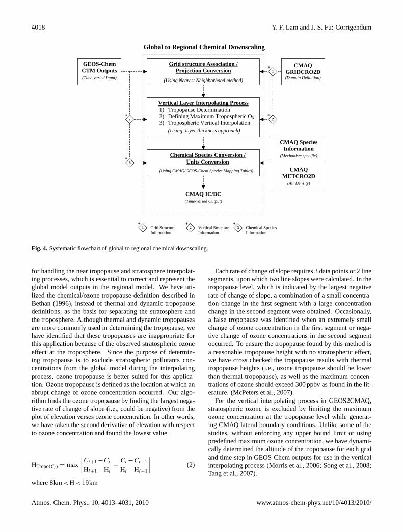
The GEOS-Chem outputs were extracted as CMAQ lat-eral boundary conditions using GEOS2CMAQ linkage tool,which involved grid structure association, horizontal/verticalinterpolation, and chemical mapping processes. A summaryof the systematic flowchart of the linkage methodology isshown in Fig. 4. It should be noted that most of the regionalmodels including CMAQ do not utilize top boundary condi-tion as input. As a result, in this study, no top boundary con-dition is generated. In the linkage process, GEOS2CMAQapplied the “nearest neighbor” method to associating thelatitude/longitude formatted GEOS-Chem outputs with theCMAQ Lambert Conformal gridded format. Horizontal in-terpolating process then utilized the results to interpolate theGEOS-Chem outputs into CMAQ gridded format for eachvertical layer column. For Tropo-BC, a newly developedtropopause-determining algorithm, which is based on chem-ical (O3) tropopause definition, was implemented in the ver-tical interpolating process to identify the tropopause height.Moreover, it separated the troposphere from the stratospherefor each horizontal grid. Different interpolating processeswere employed in the tropospheric and the stratospheric re-gions. A detailed discussion may be found in the latter sec-tion of this document. For the chemical mapping process, 38GEOS-Chem species were transformed into 24 CB-IV mech-

Table 1. MM5 and CMAQ Model Configurations for 2002 simula-tions.

MM5 Configuration

Model version 3.7Number of sigma level 34Number of grid 156×120Horizontal resolution 36 kmMap projection Lambert conformalFDDA Analysis nudgingCumulus Kain-Fritsch 2Microphysics Mix-phaseRadiation RRTMPBL Pleim-XiuLSM Pleim-Xiu LSMLULC USGS 25-Category

CMAQ Configuration

Model version 4.5Number of Layer 19Number of grid 148×112Horizontal resolution 36 kmHorizontal advection PPMVertical advection PPMAerosol module AERO3Aqueous module CB-IVEmission VISTAS emissions (NEI 2002 G)Boundary condition I CMAQ Predefined Vertical ProfileBoundary condition II 2002 GEOS-Chem

anism species of CMAQ according to the chemical defini-tions given in Appendix A. The GEOS-Chem species withthe same definitions as CB-IV species were mapped directlyinto CMAQ; where as other species were mapped by parti-tioning and/or regrouping processes. For example, total ox-idants Ox species in GEOS-Chem were defined as the com-bination of O3 and NOx. Therefore, to obtain O3 concen-trations, Ox was subtracted by NOx species in the GEOS-Chem. Other species, such as paraffin carbon bond (PAR),were composed of multiple species in GEOS-Chem. Re-grouping was required to reconstruct the CB-IV correspond-ing species, which is shown as follows:

PAR=ALK4+C2H6+C3H8+ACET+MEK+1

2PREP (1)

For chemicals that were not supported by GEOS-Chem,CMAQ predefined boundary conditions were used to main-tain the full list of CMAQ CB-IV species.

6 Tropopause determining algorithm

The newly developed tropopause-determining algorithm wasadded to the ordinary interpolating process (i.e., uses pres-sure level as the only criteria in the interpolating process)



GEOS-Chem CTM Outputs (Time-varied Input)

Global to Regional Chemical Downscaling

Grid structure Association / Projection Conversion

(Using Nearest Neighborhood method)

Vertical Layer Interpolating Process 1) Tropopause Determination 2) Defining Maximum Tropospheric O33) Tropospheric Vertical Interpolation

(Using layer thickness approach)

Chemical Species Conversion / Units Conversion

(Using CMAQ/GEOS-Chem Species Mapping Tables)

CMAQ IC/BC (Time-varied Output)

C2*

C3*

C1 C2 C3Grid Structure Information

Vertical Structure Information

Chemical Species Information

* * *

CMAQ GRIDCRO2D(Domain Definition)

C1*

C2*

CMAQ METCRO2D

(Air Density)

CMAQ Species Information

(Mechanism specific)

Fig. 4. Systematic flowchart of global to regional chemical downscaling

Fig. 4. Systematic flowchart of global to regional chemical downscaling.

for handling the near tropopause and stratosphere interpolat-ing processes, which is essential to correct and represent theglobal model outputs in the regional model. We have uti-lized the chemical/ozone tropopause definition described inBethan (1996), instead of thermal and dynamic tropopausedefinitions, as the basis for separating the stratosphere andthe troposphere. Although thermal and dynamic tropopausesare more commonly used in determining the tropopause, wehave identified that these tropopauses are inappropriate forthis application because of the observed stratospheric ozoneeffect at the troposphere. Since the purpose of determin-ing tropopause is to exclude stratospheric pollutants con-centrations from the global model during the interpolatingprocess, ozone tropopause is better suited for this applica-tion. Ozone tropopause is defined as the location at which anabrupt change of ozone concentration occurred. Our algo-rithm finds the ozone tropopause by finding the largest nega-tive rate of change of slope (i.e., could be negative) from theplot of elevation verses ozone concentration. In other words,we have taken the second derivative of elevation with respectto ozone concentration and found the lowest value.

HTropo(Ci ) = max

∣∣∣∣Ci+1−Ci

Hi+1−Hi

−Ci −Ci−1

Hi −Hi−1

∣∣∣∣ (2)

where 8km< H < 19km

Each rate of change of slope requires 3 data points or 2 linesegments, upon which two line slopes were calculated. In thetropopause level, which is indicated by the largest negativerate of change of slope, a combination of a small concentra-tion change in the first segment with a large concentrationchange in the second segment were obtained. Occasionally,a false tropopause was identified when an extremely smallchange of ozone concentration in the first segment or nega-tive change of ozone concentrations in the second segmentoccurred. To ensure the tropopause found by this method isa reasonable tropopause height with no stratospheric effect,we have cross checked the tropopause results with thermaltropopause heights (i.e., ozone tropopause should be lowerthan thermal tropopause), as well as the maximum concen-trations of ozone should exceed 300 ppbv as found in the lit-erature. (McPeters et al., 2007).

For the vertical interpolating process in GEOS2CMAQ,stratospheric ozone is excluded by limiting the maximumozone concentration at the tropopause level while generat-ing CMAQ lateral boundary conditions. Unlike some of thestudies, without enforcing any upper bound limit or usingpredefined maximum ozone concentration, we have dynami-cally determined the altitude of the tropopause for each gridand time-step in GEOS-Chem outputs for use in the verticalinterpolating process (Morris et al., 2006; Song et al., 2008;Tang et al., 2007).



0 300 600 900 1200 15000

5000

10000

15000

20000

25000

Elev

atio

n (m

)

GEOS-Chem CMAQ

North Bound

Win

ter

0 100 200 300 400

GEOS-Chem CMAQ

Tropopause region

South Bound

Sum

mer

0 300 600 900 1200 15000

5000

10000

15000

20000

25000

Elev

atio

n (m

)

GEOS-Chem CMAQ

Tropopause region0 100 200 300 400

GEOS-Chem CMAQ

Tropopause region

Tropopause region

(c) (d)

(a) (b)

O3 (ppbv) O3 (ppbv)

18*

19*

18*

19*

19*

18*

19*

18*

* CMAQ iayer no. * CMAQ layer no.

* CMAQ layer no. * CMAQ layer no.

Fig. 5. Vertical ozone profiles from GEOS-Chem plotted with GEOS-Chem and CMAQ layers for both summer and winter, (a) north bound in winter, (b) south bound in winter, (c) north bound in summer, and (d) south bound in summer

Fig. 5. Vertical ozone profiles from GEOS-Chem plotted with GEOS-Chem and CMAQ layers for both summer and winter,(a) north boundin winter, (b) south bound in winter,(c) north bound in summer, and(d) south bound in summer.

7 Results and discussion

7.1 CMAQ lateral boundary conditions

We have generated CMAQ lateral boundary conditions fromevery third hour GEOS-Chem output for VISTAS CMAQsimulation using GEOS2CMAQ linkage tool. Figure 5shows the vertical ozone profiles from GEOS-Chem withCMAQ vertical layers for both summer and winter. It shouldbe noted that the tropopause in summer is much higher thanthe tropopause in winter. As a result, less stratosphericozone is included in summer than winter when the verti-cal interpolating process is performed. In Fig. 6, compar-isons of Profile-BC, ORDY-BC, and Tropo-BC for 22 June2002 is shown on the CONUS domain. The top row rep-resents the 1st CMAQ layer (∼1000 millibars) and the bot-tom shows the top CMAQ layer (i.e., 19th layer∼140 mil-libars). These plots are intended to demonstrate the horizon-tal distribution of ozone concentrations across the CONUSdomain. The Profile-BC was designed to represent the rel-atively clean air conditions for the CONUS boundaries. Itenforces a pre-defined vertical profile with no temporal andspatial dependencies. In general, the surface ozone concen-

trations (i.e., 1st layer) range between 30 to 35 ppbv and theyprogressively increase and reache a peak ozone concentra-tion of 70 ppbv at the top (i.e., 19th layer). The ORDY-BC and Tropo-BC were both generated using the linkagemethodology described earlier. This methodology intendsto incorporate the effects of intercontinental transport of airpollutants and the rise in background ozone concentrationsinto CMAQ by utilizing GEOS-Chem outputs. (Bertschi etal., 2004; Fiore et al., 2003; Park et al., 2004) The tempo-ral and horizontal variations in GEOS-Chem were capturedinto CMAQ to reflect daily diurnal differences in concentra-tions. In ORDY-BC and Tropo-BC, the difference was thevertical interpolating process. ORDY-BC uses the ordinaryvertical interpolating process, where as Tropo-BC uses theordinary vertical interpolating process with the tropopause-determining algorithm that excludes pollutants in the strato-sphere from the interpolating process. In the surface level(1st layer), both ORDY-BC and Tropo-BC perform identi-cally; ozone concentrations ranged from 19 ppbv to 90 ppbvdepending on location and time on June 22nd. For otherdays in 2002 (i.e., January, June, and July), ozone concen-tration could reach up to 130 ppbv at the surface. In the toplevel (19th layer), the ORDY-BC ozone reaches as much as



b) c) a)

19th layer

1st layer

Fig. 4. Comparison of different lateral boundary conditions in 1st and 19th layers, a) Profile-BC, b) ORDY-BC, and c) Tropo-BC.

Fig. 6. Comparison of different lateral boundary conditions in 1st and 19th layers,(a) Profile-BC,(b) ORDY-BC, and(c) Tropo-BC.

235 ppbv and the Tropo-BC ozone achieves up to 160 ppbvin the CONUS domain on 22nd June. For other days in 2002,the ORDY-BC and Tropo-BC ozone reaches up to 714 ppbvand 205 ppbv, respectively. In Considine (2008), the re-ported maximum mean tropopause ozone concentration fromobservations in North America is about 235 ppbv based onthe thermal tropopause definition. We would have expectedthat if Considine’s analyses used the ozone tropopause as itsdefinition, the maximum tropopause ozone concentrationsshould be lower since the ozone tropopause is constantlylower than the thermal tropopause at the upper troposphere.So, the maximum ORDY-BC ozone of 714 ppbv would betoo high in the troposphere and would impractically bringhigh ozone to surface level, where as the maximum Tropo-BC ozone of 205 ppbv has fallen within a reasonable valuein the United States. It should be noted that the Considine’sdata is concentration at higher latitudinal locations. With thedirect proportional relationship between latitudinal locationand tropopause ozone concentration, we would expect thatthe reported 235 ppbv should be a high end of the ozone con-centration at the tropopause in the United States.

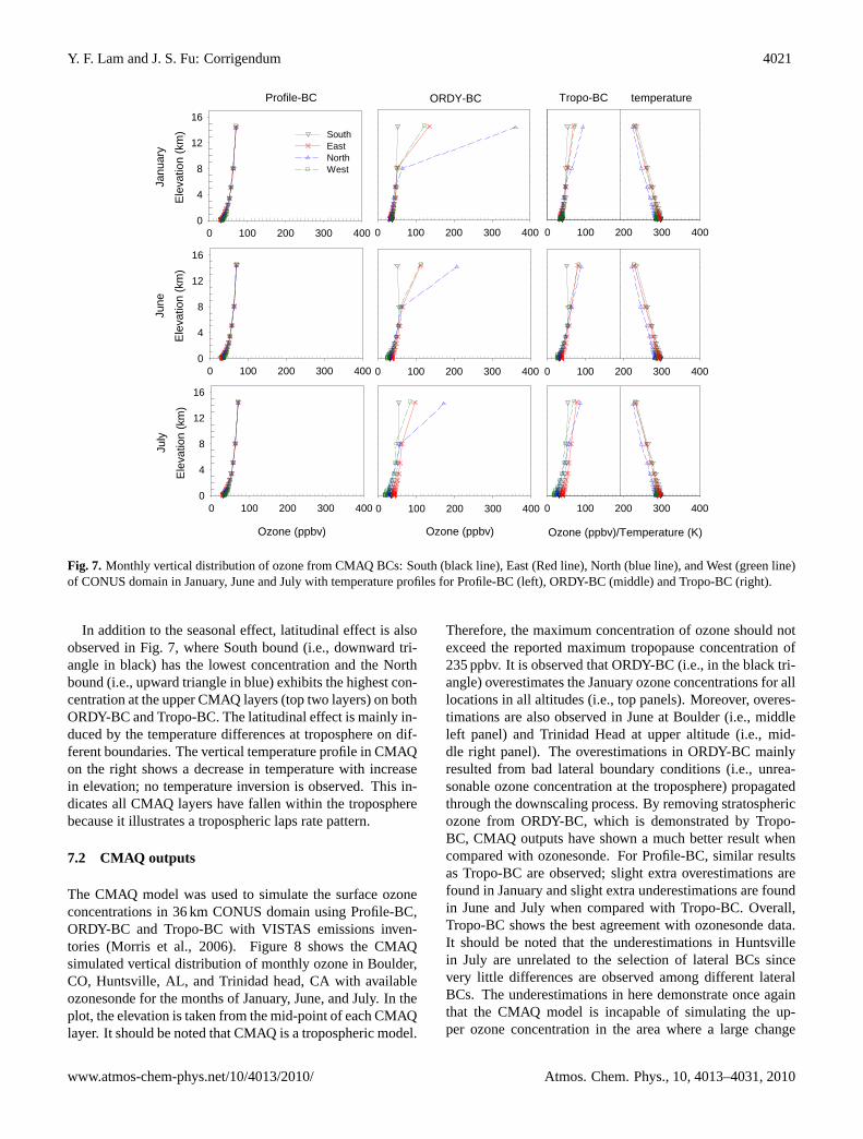
As tests of the lateral boundary conditions’ responses tothe GEOS2CMAQ linkage tool, we have extracted the ver-tical profiles of various CMAQ boundary conditions for se-lected months to investigate the seasonal effects of the data.Figure 7 shows average monthly ozone vertical distributionfrom all four boundaries of the CONUS domain: East, West,South, and North are shown in various colors with averagevertical temperature profiles for January, June, and July. Jan-uary represents the winter condition where tropopause is rel-atively low as a consequence of cold temperatures; July char-acterizes the summer condition with possible high surface

ozone concentration. The additional month of June is se-lected because we have occasionally observed high effectsof stratospheric ozone to the surface ozone from the MISC-ASIA study (Fu et al., 2008). As expected, Profile-BC onthe left has shown no seasonal variation. In contrast, theORDY-BC and Tropo-BC are both showing a seasonal de-pendence. The ORDY-BC in the middle panel has shown astrong seasonal difference at the top CMAQ layer (i.e., blueline). This dependence directly relates to the seasonal dif-ference in ozone tropopause heights as a result of tempera-ture differences. In the ORDY-BC interpolating process, theamount of stratospheric ozone included in boundary condi-tions is governed by the altitude of ozone tropopause. It ishighly sensitive with elevation because ozone is exponen-tially increased with altitude beyond tropopause or at strato-sphere. The vertical structures of CMAQ and GEOS-Chemare also playing an important role. With the constant eleva-tions in CMAQ layers, the higher the tropopause is located,the less stratospheric effect will result. As shown in Fig. 7,the monthly average ozone concentrations for ORDY-BC onNorth bound at the top CMAQ layer for January, June, andJuly are 362 ppbv, 207 ppbv, and 172 ppbv, respectively. Asrecalled from early comparisons with Considine (2008), thisaverage concentration in January is too high. For Tropo-BC,shown on the right panel, little seasonal variation is observedat the top CMAQ layer. The average monthly ozone concen-trations of 94 ppbv, 90 ppbv, and 86 ppbv are found on theNorth bound for January, June, and July, respectively. Theseresults demonstrate the effects of tropopause-determining al-gorithm, which have limited the stratospheric effects fromthe BCs.



0 100 200 300 4000

4

8

12

16

0 100 200 300 4000 100 200 300 400

SouthEastNorthWest

Ele

vatio

n (k

m)

Janu

ary

0 100 200 300 4000

4

8

12

16

0 100 200 300 4000 100 200 300 400

Ele

vatio

n (k

m)

June

0 100 200 300 4000 100 200 300 4000

4

8

12

16

Ele

vatio

n (k

m)

July

0 100 200 300 400

Ozone (ppbv) Ozone (ppbv) Ozone (ppbv)/Temperature (K)

Profile-BC ORDY-BC Tropo-BC temperature

Fig. 5. Monthly vertical distribution of ozone from CMAQ BCs: South (black line), East (Red line), North (blue line), and West (green line) of CONUS domain in January, June and July with temperature profiles for Profile-BC (left), ORDY-BC (middle) and Tropo-BC (right).

Fig. 7. Monthly vertical distribution of ozone from CMAQ BCs: South (black line), East (Red line), North (blue line), and West (green line)of CONUS domain in January, June and July with temperature profiles for Profile-BC (left), ORDY-BC (middle) and Tropo-BC (right).

In addition to the seasonal effect, latitudinal effect is alsoobserved in Fig. 7, where South bound (i.e., downward tri-angle in black) has the lowest concentration and the Northbound (i.e., upward triangle in blue) exhibits the highest con-centration at the upper CMAQ layers (top two layers) on bothORDY-BC and Tropo-BC. The latitudinal effect is mainly in-duced by the temperature differences at troposphere on dif-ferent boundaries. The vertical temperature profile in CMAQon the right shows a decrease in temperature with increasein elevation; no temperature inversion is observed. This in-dicates all CMAQ layers have fallen within the tropospherebecause it illustrates a tropospheric laps rate pattern.

7.2 CMAQ outputs

The CMAQ model was used to simulate the surface ozoneconcentrations in 36 km CONUS domain using Profile-BC,ORDY-BC and Tropo-BC with VISTAS emissions inven-tories (Morris et al., 2006). Figure 8 shows the CMAQsimulated vertical distribution of monthly ozone in Boulder,CO, Huntsville, AL, and Trinidad head, CA with availableozonesonde for the months of January, June, and July. In theplot, the elevation is taken from the mid-point of each CMAQlayer. It should be noted that CMAQ is a tropospheric model.

Therefore, the maximum concentration of ozone should notexceed the reported maximum tropopause concentration of235 ppbv. It is observed that ORDY-BC (i.e., in the black tri-angle) overestimates the January ozone concentrations for alllocations in all altitudes (i.e., top panels). Moreover, overes-timations are also observed in June at Boulder (i.e., middleleft panel) and Trinidad Head at upper altitude (i.e., mid-dle right panel). The overestimations in ORDY-BC mainlyresulted from bad lateral boundary conditions (i.e., unrea-sonable ozone concentration at the troposphere) propagatedthrough the downscaling process. By removing stratosphericozone from ORDY-BC, which is demonstrated by Tropo-BC, CMAQ outputs have shown a much better result whencompared with ozonesonde. For Profile-BC, similar resultsas Tropo-BC are observed; slight extra overestimations arefound in January and slight extra underestimations are foundin June and July when compared with Tropo-BC. Overall,Tropo-BC shows the best agreement with ozonesonde data.It should be noted that the underestimations in Huntsvillein July are unrelated to the selection of lateral BCs sincevery little differences are observed among different lateralBCs. The underestimations in here demonstrate once againthat the CMAQ model is incapable of simulating the up-per ozone concentration in the area where a large change



0 40 80 120

Elev

atio

n (k

m)

0

4

8

12

Ozone (ppbv)

0 40 80 120

Elev

atio

n (k

m)

0

4

8

12

0 40 80 120

Elev

atio

n (k

m)

0

4

8

12

0 40 80 120

0 40 80 120

0 40 80 120 0 40 80 120

0 40 80 120

0 40 80 120

Ozone (ppbv) Ozone (ppbv)

(40.0N, 105.25W) (34.7N, 86.61W) (41.05N, 124.15W)

JAN

JUN

JUL

Boulder, CO Huntsville, AL Trinidad Head, CA

Ozonesonde Profile-BC Tropo-BC ORDY-BC

Fig. 6. CMAQ simulated monthly vertical distribution of ozone for Profile-BC (red line), Tropo-BC (blue line) and ORDY-BC (black line) with ozonesonde.

Fig. 8. CMAQ simulated monthly vertical distribution of ozone for Profile-BC (red line), Tropo-BC (blue line) and ORDY-BC (black line)with ozonesonde.

of upper ozone concentration occurred. We believe that thismay be resolved if CMAQ can implement the STE mech-anism along with supplementary upper boundary conditionfrom GCM.

Figures 9 and 10, respectively, show the outputs of the av-erage monthly surface ozone concentrations and the maxi-mum monthly surface ozone concentrations for January (topframes), June (middle frames), and July (bottom frames).The maximum ozone concentrations within the domain arealso listed at the corner and denoted in blue or white. InFig. 9, the output results show that similar ozone concentra-tion patterns are found across the CONUS domain among allthree BCs with some exceptional high ozone being observedin the ORDY-BC. It is believed that these high ozone concen-trations occurring in the Western United States in ORDY-BCare the consequence of high ozone observed at the top layerof CMAQ boundaries discussed earlier. The undesirableboundary conditions (i.e., ORDY-BC) produce abnormal sur-

face ozone concentrations for both January and June. Sinceozone is a photochemical pollutant driven by NOx, VOCs,and temperature, we would expect higher monthly averageozone should be observed in July rather than in January. Inthe top frames, the reported maximum average ozone con-centrations in January for Profile-BC, ORDY-BC, and Tropo-BC are 55 ppbv, 69 ppbv, and 50 ppbv, respectively. A similartrend is observed for June. For July (bottom frames), the ef-fects of stratospheric ozone in ORDY-BC become minimaldue to the fact that the tropopause is much higher than othermonths at the top layer. As a result, fewer differences arefound among these three scenarios. Figure 10 shows that themonthly maximum 8-h ozone concentration in January onORDY-BC is in excess of 150 ppbv over the western UnitedStates. The result indicates that the effect of stratosphericozone in lateral boundary conditions has a significant im-pact on surface ozone concentrations, as a result of the highozone aloft mixing downward quickly. The large differences



Janu

ary

June

July

Max = 55 ppb

Max = 62 ppb

Max = 66 ppb

Max = 55 ppb

Max = 62 ppb

Max = 66 ppb

Max = 50 ppb

Max = 64 ppb

Max = 66 ppb

Max = 50 ppb

Max = 64 ppb

Max = 66 ppb

Max = 69 ppb

Max = 70 ppb

Max = 69 ppb

Max = 69 ppb

Max = 70 ppb

Max = 69 ppb

a) b) c)

Fig. 7. Comparisons of monthly average ozone concentrations in January, June and July from CMAQ outputs; a) Profile-BC (left), b) ORDY-BC (middle), and c) Tropo-BC (right). The maximum concentration within the domain is shown at the bottom of right hand corner.

Fig. 9. Comparisons of monthly average ozone concentrations in January, June and July from CMAQ outputs;(a) Profile-BC (left), (b)ORDY-BC (middle), and(c) Tropo-BC (right). The maximum concentration within the domain is shown at the bottom of right hand corner.

Janu

ary

June

July

a) b) c)

Max = 75 ppb

Max = 165 ppb

Max = 200 ppb

Max = 75 ppb

Max = 165 ppb

Max = 200 ppb

Max = 151 ppb

Max = 179 ppb

Max = 201 ppb

Max = 151 ppb

Max = 179 ppb

Max = 201 ppb

Max = 66 ppb

Max = 169 ppb

Max = 199 ppb

Max = 66 ppb

Max = 169 ppb

Max = 199 ppb

Fig. 8. Comparisons of monthly maximum 8-hour surface ozone concentrations in January, June and July from CMAQ outputs; a) Profile-BC (left), b) ORDY-BC (middle), and c) Tropo-BC (right). The maximum concentration within the domain is shown at the bottom of right hand corner.

Fig. 10.Comparisons of monthly maximum 8-h surface ozone concentrations in January, June and July from CMAQ outputs;(a) Profile-BC(left), (b) ORDY-BC (middle), and(c) Tropo-BC (right). The maximum concentration within the domain is shown at the bottom of righthand corner.



Fig. 9. Comparison of simulated and measured surface ozone concentration for month of January, June and July from the selected sites. The quoted value at the bottom of each plot revives the root mean square error of each case.

Fig. 11. Comparison of simulated and measured surface ozone concentration for month of January, June and July from the selected sites.The quoted value at the bottom of each plot revives the root mean square error of each case.

observed between ORDY-BC and Profile-BC/Tropo-BC re-veal an important message, which is “excluding stratosphericozone on tropospheric model during the downscaling pro-cess is extremely important. We have found the concentra-tion differences between these scenarios could be as muchas 87 ppbv in January. These differences gradually decreasewith temperature increasing through June and July. The ef-fects of lateral BCs in ORDY-BC have contributed to the highsurface concentrations observed in the western United Statesin January and June. Since both ORDY-BC and Tropo-BCutilize a dynamic algorithm to interpolate the vertical ozoneprofile for each horizontal grid for lateral BCs, the variationsin the western boundary are observed primarily due to thetreatments of stratospheric ozone. Note that the Tropo-BC isintended to demonstrate the effectiveness of the tropopause-determining algorithm of separating the stratospheric andtropospheric ozone for the lateral boundary condition.

7.3 CMAQ performance analyses

Model performance analyses on all three cases have beenperformed using the entire CASTNET dataset, in which 70+observation sites across the CONUS domain from both EPA

and the National Park Service (NPS) are included. It shouldbe noted that our study only simulates the 36 km domain andit is intended to demonstrate the effects of different BCs.Hence, the results in root mean square error in this researchmay be higher than the one in a finer resolution CMAQ. Fig-ure 11 shows the simulated and measured surface ozone forthe months of January, June, and July at the nearest loca-tions of the ozonesonde sites found in CASTNET network(see Fig. 3 denoted in red star). In the plot, blue, purple,green, and red colors correspond to observation, Profile-BC,ORDY-BC, and Tropo-BC, respectively. And the top, mid-dle, and bottom panels show the first 15 day’s outputs for Jan-uary, June, and July, respectively. It should be noted that, dueto limitation of the size of the plot, we have only documentedthe first 15 days of data in Fig. 11. However, our analysesare based on a full month of data. The quoted number be-low each point represents root mean square error (RMSE)for each case, with the same color scheme used on the plot.

7.3.1 ORDY-BC

In these time series plots, we, once again, found the sur-face ozone in ORDY-BC is over predicted in January and



a) b)

NET-RMSE Predicted (ppbv)

0 5 10 15 20 25 30

NE

T-R

MS

E A

ctua

l (pp

bv)

0

5

10

15

20

25

30

JanuaryJuneJune<252K July

JAN: NET-RMSE=459.7-1.59(Avg_temp) -1.69(LAT), R2=0.73

JUL: RMSE=6.73-0.02(Avg_temp), R2=0.01JUN<252: NET-RMSE=203.9-0.81(Avg_temp), R2=0.52JUN: NET-RMSE=108.87-0.42(Avg_temp), R2=0.3

Temperature (K)

248 250 252 254 256 258 260

RM

SE (p

pbv)

/ R

2

0.0

0.5

1.0

1.5

2.0

2.5

3.0

R2

RMSE

Fig. 10. Statistical analysis outputs from CASTNET sites: a) NET-RMSE actual Vs. NET-RMSE predicted, b) sensitivity analysis on best-fit equation for June data.

Fig. 12. Statistical analysis outputs from CASTNET sites:(a) NET-RMSE actual vs. NET-RMSE predicted,(b) sensitivity analysis onbest-fit equation for June data.

June (i.e., top and middle panels) and it is in agreementwith our results early in Fig. 10. In comparisons of RMSE,ORDY-BC has shown the worst prediction of surface ozonecomparing with others. The RMSE reaches as much as23.0 ppbv. The highest RMSE occurs at the conditions wherethe tropopause is low in January and at “near Boulder” site(top left panel). This large RMSE strongly ties to the pa-rameters such as air temperature, altitudinal, and latitudinallocations. Since “near Boulder” is located much higher in al-titude (i.e., Boulder at about 1650 m above mean sea level)than Huntsville and Trinidad head, the larger amount andquicker downshift of uncontrolled stratospheric ozone is ex-pected at the surface of ORDY-BC. This did not happen inProfile-BC and Tropo-BC since both of them do not con-tain any stratospheric ozone. For air temperature, Januaryhas much lower air temperature than June and July. Withthe relationship of air temperature, it is directly proportionalto tropopause height; lower air temperature means a lowertropopause height. Therefore, a larger amount of aloft ozoneis included in the lateral boundary condition of ORDY-BCand results from a huge over prediction of surface ozone in“near Boulder”. This low temperature effect has also con-tributed to the high RMSE found in “near Huntsville” and“near Trinidad head” sites in January.

Another high RMSE(s) is found in “near Boulder” and“near Trinidad head” in June. These high RMSE(s) mostlikely relate to the low tropopause height resulting from lowair temperature. We believe latitudinal location might ex-plain why “near Boulder” and “near Trinidad head” observedhigh RMSE, where as “near Huntsville” did not. In gen-eral, the higher latitudinal location is, the lower temperaturewill be when it is further away from the equator. The lowtemperature condition affects the downscaling process by

changing the tropopause height and resulting in more strato-spheric ozone in the lateral boundary conditions in ORDY-BC. To demonstrate the effect of tropopause due to air tem-perature and latitudinal location, we calculated the RMSEin all CASTNET sites for each boundary condition. More-over, we subtracted the RSME in ORDY-BC to the RSME inTropo-BC to yield a net RSME to account for stratosphericozone effect, denoted as NET-RSME. Note that the differ-ence between ORDY-BC and Tropo-BC is the extra strato-spheric concentrations from GEOS-Chem. Therefore, weuse the differences in RMSE as an indicator for stratosphericeffects on surface ozone performance. Multivariate statisti-cal fitting is performed on NET-RMSE with monthly aver-age column temperature and latitudinal location. Figure 12shows the results from statistical analyses: (a) multivariatefitting for NET-RMSE on each month, (b) sensitivity analy-sis on multivariate fitting for the month of June. Note thatthe equations on top of Fig. 12a are the best-fit equationsfor temperature and latitude. These equations are used togenerate the NET-RMSE predicted in Fig. 12 (a) and theydo not represent the best-fit equations for the straight linesshown in Fig. 12a. For January, NET-RMSE is highly corre-lated with latitudinal location and air temperature withR2

of 0.73 and RMSE of 2.73. For June, only air tempera-ture is correlated to NET-RMSE withR2 of 0.3. And forJuly, no correlation is found on either latitudinal locationor air temperature. Since NET-RMSE is an indicator of thestratospheric effect from the lateral BCs, we believed that nocorrelation observed in July implies the average column airtemperature has reached a certain level at which tropopauseheight is higher than the upper boundary of CMAQ. Thus,no stratospheric ozone is included in the lateral BCs. To de-termine the temperature at which there is no stratospheric



Table 2. Summary of NET-RMSE and average column temperatures for the sonde sites.

Boulder, CO Huntsville, AL Trinidad head, CA

January Tc = 236 K Tc = 246 K Tc = 242 KNET-RMSE = 10.5 ppbv NET-RMSE = 11.4 ppbv NET-RMSE = 6.9 ppbv

June Tc = 247 K Tc = 254 K Tc = 252 KNET-RMSE = 6.5 ppbv NET-RMSE = 1.4 ppbv NET-RMSE = 7.9 ppbv

July Tc = 253 K Tc = 257 K Tc = 255 KNET-RMSE = 0.39 ppbv NET-RMSE = 1.0 ppbv NET-RMSE = 0.1 ppbv

Tc is average vertical column temperature; NET-RMSE is the RMSE differences between Profile-BC and Tropo-BC.

effect, we have performed sensitive fittings on June’s databecause it contains both stratospheric effect sites and non-stratospheric effect sites. Figure 12b shows the results ofthe sensitive test and the observed break point temperatureis about 252 K, at which the lowest RMSE and the highestR2 are obtained. These results are consistent with our earlyexplanations of why bad predictions of ORDY-BC occurredin January and June and similar predictions as Tropo-BC arefound in July. Table 2 shows the monthly average columntemperature along with NET-RMSE in all three ozonesondesites for all months. For January, all three sites have the av-erage temperature lower than 252 K. Therefore, a large NET-RMSE caused from stratospheric ozone is expected. ForJune, Boulder and Trinidad head are equal or below 252 K,where as Huntsville is above 252 K. Hence, a large NET-RMSE(s) is observed in those two sites and a small NET-RMSE is found in Huntsville. These results are in agreementwith our conclusions made earlier on the time-series plotsin Fig. 11. Overall, these results stress the important rela-tionship of temperature and seasonal changes in the GCMdownscaling process.

7.3.2 Profile-BC

For Profile-BC versus lateral boundary conditions fromGCTM, Tang et al. (2007, 2009), have found that the perfor-mance of boundary conditions from GCTM may not neces-sarily be better than Profile-BC. Moreover, different GCTMoutputs also yield different results. The performance of lat-eral boundary conditions from GTCM (GCTM-LBC) highlydepends on locations and scenarios of the GCTM-LBC, alsothe type of GCTM used. Al-Saadi et al. (2007), suggestedthat this phenomenon might relate to the ozone aloft inGCTM-LBC, where rapid transports of stratospheric ozoneinto the surface level are observed. In addition, they havefound that GCTM-LBC enhances the model errors of ozoneconcentration at the surface in the range of 6 to 20 ppbvin Trinidad Head in August. Since these studies have se-lected the summer ozone season (i.e., August) as their studyperiod, we expected that the effect of stratospheric ozonewould be minimal based on the relationship we developedearlier. However, this did not happen. In this case, we sus-

pect their average column temperature in August for Trinidadhead may not be hot enough to exclude the stratosphericozone from the GCTM-LBC interpolating process, or it maybe affected by the quality of GCTM-LBC as inputs wherestrong boundary influx of ozone affects the simulation re-sults. Nevertheless, these studies have indicated that GCTM-LBC preprocessing may be required. In our study, we haveimplemented the tropopause-determining algorithm, whichis based on chemical tropopause definition, as the prepro-cessor for generating ORDY-BC and denoted at Tropo-BC.Note that ORDY-BC is one kind of GCTM-LBC. The inten-tion of the tropopause algorithm is an attempt to improve theozone simulation at the surface. Figure 11 shows the RMSEfor both Profile-BC and Tropo-BC. The results show thatthe RMSE in Profile-BC is always higher than the RMSEin Tropo-BC, where as the ORDY-BC have either greateror less than Profile BC depending on the locations. Al-though the differences between Profile-BC and Tropo-BC inRMSE was found to be within 1 to 2 ppbv in June and July,and 3 to 4 ppbv in January, the results have demonstratedthe tropopause-determining algorithm has successfully pre-vented the high surface ozone estimates, which Tang and Al-Saadi mentioned in their study.

7.3.3 Tropo-BC

For overall performance of Tropo-BC, we have included ad-ditional statistical analyses using all CASTNET data. Ta-ble 3 shows the summary of RMSE and mean bias (MB)for all three BCs. In the table, we have broken downthe entire United States into three regions, which are WestCoast (West), Central United States (Central), and East Coast(East). The average RMSE for all three months in all stationsis calculated to be 14.2 ppbv, 13.3 ppbv, and 17.6 ppbv forProfile-BC, Tropo-BC, and ORDY-BC, respectively. We ob-served that the RMSE in Tropo-BC is always lower than bothProfile-BC and ORDY-BC for every region and every month.This demonstrates the Tropo-BC is the best method of gen-erating lateral boundary condition for CMAQ. In the table,large differences (i.e., average in 3 ppbv) between Tropo-BCand Profile-BC are observed in the “West”. It should be notedthat this large RMSE improvement in the “West” was mainly



Table 3. Summary of NET-RMSE and average column temperatures for the sonde sites.

Profile-BC Tropo-BC ORDY-BC

January All RMSE = 11.9 ppbv RMSE = 10.3 ppbv RMSE = 19.8 ppbvMB = 7.3 ppbv MB = 3.9 ppbv MB = 13.2 ppbv

West RMSE = 16.8 ppbv RMSE = 13.0 ppbv RMSE = 23.5 ppbvMB = 14.6 ppbv MB = 9.8 ppbv MB = 18.3 ppbv

Central RMSE = 10.1 ppbv RMSE = 8.2 ppbv RMSE = 23.6 ppbvMB = 6.6 ppbv MB = 2.4 ppbv MB = 16.1 ppbv

East RMSE = 11.2 ppbv RMSE = 10.1 ppbv RMSE = 18.0 ppbvMB = 6.3 ppbv MB = 3.2 ppbv MB = 11.5 ppbv

June All RMSE = 14.3 ppbv RMSE = 13.8 ppbv RMSE = 16.4 ppbvMB = 0.3 ppbv MB = 1.9 ppbv MB = 7.2 ppbv


Central RMSE = 12.5 ppbv RMSE = 11.3 ppbv RMSE = 16.0 ppbvMB = −4.5 ppbv MB =−1.3 ppbv MB = 6.1 ppbv


July All RMSE = 16.3 ppbv RMSE = 15.8 ppbv RMSE = 16.6 ppbvMB = 4.2 ppbv MB = 3.4 ppbv MB = 5.3 ppbv


Central RMSE = 13.7 ppbv RMSE = 13.3 ppbv RMSE = 13.7 ppbvMB = −2.4 ppbv MB =−3.1 ppbv MB =−1.4 ppbv


All – All stations; West – West of 115 W; Central – Between 115 W and 94 W; East – East of 94 W;RMSE is root mean square error; MB is mean bias.

contributed by the sites that are located in the State of Wash-ington. The magnitude of changing RMSE in the State ofWashington ranges from 4 to 12 ppbv. The poor performanceof Profile-BC in RMSE in the “West” has shown that Profile-BC has failed to estimate the impact from intercontinentaltransport of air pollutants from East Asia across the PacificOcean. Moreover, it fails to represent the actual geospatialvariations of lateral boundary in the United States.

For the performance of Tropo-BC in all other regions, mi-nor improvement is observed when compared with Profile-BC. Large improvement is found in month of January. SinceProfile-BC uses a fixed BC concentration and this fixed BCconcentration is usually higher than the actual backgroundozone in winter, as a result, overestimation of surface ozonein Profile-BC is observed. This demonstrates the importanceof using dynamic BCs instead of the static BCs. Figure 13shows the distributions of RMSE differences among thesethree scenarios for each of the CASTNET sites. If we con-sider ±1 ppbv as model variability, then we conclude thatonly 5% or less of the sites in Tropo-BC have poorer perfor-mance compared with Profile-BC. In these 5% of the sites,we have observed the Tropo-BC overestimated the nighttimeozone concentration in June.

In comparison with ORDY-BC, Tropo-BC is outper-formed for every observation site in January. Strong im-provement in Tropo-BC is found in both January and June.In the plot, we have observed 10% or less of the sites inTropo-BC have poorer performance than in ORDY-BC (i.e.,right side panel). We believed that this 10% is contributed bythe nature of underestimation of ozone in 36 km resolution.Since the surface ozone in ORDY-BC is always higher thanin Tropo-BC, the improvement may not actually be counted.For the overall performance, Tropo-BC has outperformedORDY-BC in every month for all regions. These results,once again, demonstrate that the removal of stratosphericozone using our tropopause-determining algorithm stronglyimproves the performance of surface ozone simulations inCMAQ.

8 Conclusion

In this study, we have successfully integrated our newly de-veloped tropopause-determining algorithm, based on chemi-cal tropopause definition, into the methodology of downscal-ing from the global chemical model (i.e., GEOS-Chem) intothe regional air quality model (i.e., CMAQ). The purposeof the algorithm is to resolve the inconsistency of vertical



- 4 0 4 8 12 16 20 24

-4 0 4 8 12 16 20 24

510

1520

510

20

30

-2 0 2 4 6 8 10 12

-4 0 4 8 12 16 20 24

5

10

15

-2 0 2 4 6 8 10 12

-2 0 2 4 6 8 10 12

JUN

JAN

JUL

Cou

ntC

ount

Cou

nt

Profile-BC - Tropo-BC

RMSE (ppbv)

10

20

3040

5101520

2468

ORDY-BC - Tropo-BC

RMSE (ppbv)

Fig. 11. Summary of the RMSE distributions for the differences among these three scenarios for each CASTNET sites.

Fig. 13. Summary of the RMSE distributions for the differences among these three scenarios for each CASTNET sites.

structures between GEOS-Chem (i.e., containing both thetropospheric and stratospheric components) and CMAQ(containing only the tropospheric component). It identifiesthe height of tropopause from GCTM outputs and appliestropopause ozone concentration as the maximum ozone con-centration at the CMAQ lateral boundary condition. As a re-sult, it excludes any stratospheric ozone from being includedin the regional air quality model. Since CMAQ is only de-signed for tropospheric application with no top boundary in-put, any stratospheric ozone or stratospheric intrusion shouldbe considered inapplicable in CMAQ. In our results, we havefound that the GCTM output (i.e., GEOS-Chem) with thetropopause-determining algorithm (i.e., Tropo-BC) alwaysyields a better result than that with the fixed BCs (i.e., Profile-BC). Moreover, Tropo-BC also yields better results than thatwith the GCM BCs (i.e., ORDY-BC). For Profile-BC, wehave observed the fixed BCs tend to overestimate surfaceozone concentration during wintertime and underestimate insummertime. For ORDY-BC, strong over prediction of sur-face ozone is observed as a result of stratospheric ozone fromthe upper atmosphere. These results are similar to the find-ings in Tang et al., where a large overestimation is observedin CMAQ surface ozone when applying GCTM-BC. Fortu-nately, using our new tropopause algorithm technique (i.e.,Tropo-BC) with the global model input (i.e., GEOS-Chem),we have resolved the high surface ozone issue observed inGCTM-BC, while maintaining good vertical ozone predic-tion in the upper air. For further improving the model simu-lations, we recommended that all vertical layers from MM5

(i.e., 34 layers) should be used in CMAQ, instead of 19 layerscreated from vertical collapsing. This way, it will break downthe original CMAQ top layer into 5 separated layers with athickness of 1.0 to 1.5 km for vertical transport. It is believedthat the top CMAQ layer (i.e., 6 km deep) is relatively toothick; it may give a wrong representation of transport of fluxin the upper troposphere.

In statistical analysis, we have performed a correlationstudy on the average tropospheric column temperature andstratospheric effect using the RMSE differences betweenORDY-BC and Tropo-BC. The results show that a breakpoint temperature, which separates the temperature regionbetween stratospheric effect and non-stratospheric effect inthe chemical downscaling process, is about 252 K. This valuecan be used as a quick check to see whether or not a partic-ular region or day in the regional model is having a strato-spheric effect from GCTM-BC. Nevertheless, this tempera-ture is based on statistical analysis and may contain certainstatistical errors. Therefore, we recommend only using thisvalue as a screening tool.

In conclusion, we have demonstrated the advantage of us-ing the tropopause-determining algorithm along with time-varying GCTM lateral BC for air quality predictions of thetropospheric ozone. We have advanced the exiting techniqueon how GCTM data can be incorporated into CMAQ lateralBC. This methodology can be applied on different GCTMdata for downscaling purposes to yield a better surface ozoneprediction in a regional CTM.



Appendix A

GEOS-Chem to CMAQ IC/BC species mappingtable

CMAQ CB-IV species GEOS-CHEM species

[NO2] [NOx]

[O3] [Ox]-[NOx]

[N2O5] [N2O5]

[HNO3] [HNO3]

[PNA] [HNO4]

[H2O2] [H2O2]

[CO] [CO]

[PAN] [PAN] + [PMN] + [PPN]

[MGLY ] [MP]

[ISPD] [MVK ] + [MACR]

[NTR] [R4N2]

[FORM] [CH2O]

[ALD2] 1/2[ALD2] + [RCHO]

[PAR] [ALK4 ] + [C2H6] + [C3H8] +[ACET] + [MEK] + 1/2 [PRPE]

[OLE] 1/2 [PRPE][ISOP] 1/5 [ISOP][SO2] [SO2]

[NH3] [NH3]

[ASO4J] [SO4]

[ANH4J] [NH4]

[ANO3J] [NIT] + [NITs][AECJ] [BCPI] + [BCPO]

[AORGPAJ] [OCPI] + [OCPO]

[AORGBJ] [SOA1]+[SOA2]+[SOA3]+[SOA4]

Acknowledgements.This work was supported by the US Environ-mental Protection Agency under STAR Agreement R830959 andthe Intercontinental transport and Climatic effects of Air Pollutants(ICAP) project. It has not formally been reviewed by the EPA.The views presented in this document are solely those of theauthors and the EPA does not endorse any products or commercialservices mentioned in this publication. We also thank NSF fundedNational Institute of Computational Sciences for us to use Krakensupercomputer on this study.

Edited by: F. Dentener

References

Al-Saadi, J., Pierce, B., McQueen, J., Natarajan, M., Kuhl, D.,Tang, Y. H., Schaack, T. K., and Grell, G.: Global ForecastingSystem (GFS) Project: Improving National chemistry forecast-ing and assimilation capabilities, Applications of EnvironmentalRemote Sensing to Air Quality and Public Health, Potomac, MD,8–9 May 2007.

Bertschi, I. T., Jaffe, D. A., Jaegle, L., Price, H. U., and Den-nison, J. B.: 2002 airborne observations of trans-Pacific trans-port of ozone, CO, volatile organic compounds, and aerosols

to the northeast Pacific: Impacts of Asian anthropogenic andSiberian boreal fire emissions, J. Geophys. Res., 109, D23S12,doi:10.1029/2003JD004328, 2004.

Bethan, S., Vaughan, G., and Reid, S. J.: A comparison of ozoneand thermal tropopause heights and the impact of tropopause def-inition on quantifying the ozone content of the troposphere, Q. J.Roy. Meteor. Soc., 122, 929–944, 1996.

Byun, D. and Schere, K. L.: Review of the governing equations,computational algorithms, and other components of the models-3 Community Multiscale Air Quality (CMAQ) modeling system,Appl. Mech. Rev., 59, 51–77, 2006.

Byun, D. W., Moon, N. K., Jacob, D., and Park, R.: Regional trans-port study of air pollutants with linked global tropospheric chem-istry and regional air quality models, 2nd ICAP Workshop, Re-search Triangle Park, NC, USA, 2004.

Chin, M., Diehl, T., Ginoux, P., and Malm, W.: Intercontinentaltransport of pollution and dust aerosols: implications for regionalair quality, Atmos. Chem. Phys., 7, 5501–5517, 2007,http://www.atmos-chem-phys.net/7/5501/2007/.

Collins, W. J., Derwent, R. G., Garnier, B., Johnson, C. E.,Sanderson, M. G., and Stevenson, D. S.: Effect of stratosphere-troposphere exchange on the future tropospheric ozone trend,J. Geophys. Res., 108(D12), 8528, doi:10.1029/2002JD002617,2003.

Eder, B., and Yu, S. C.: A performance evaluation of the 2004release of Models-3 CMAQ, Atmos. Environ., 40, 4811–4824,2006.

Fiore, A., Jacob, D. J., Liu, H., Yantosca, R. M., Fairlie, T. D.,and Li, Q.: Variability in surface ozone background over theUnited States: Implications for air quality policy, J. Geophys.Res., 108(D24), 4787, doi:10.1029/2003JD003855, 2003.

Fu, J. S., Jang, C. J., Streets, D. G., Li, Z. P., Kwok, R., Park, R.,and Han, Z. W.: MICS-Asia II: Modeling gaseous pollutants andevaluating an advanced modeling system over East Asia, Atmos.Environ., 42, 3571–3583, 2008.

Fusco, A. C. and Logan, J. A.: Analysis of 1970-1995 trends intropospheric ozone at Northern Hemisphere midlatitudes withthe GEOS-CHEM model, J. Geophys. Res., 108(D15), 4449,doi:10.1029/2002JD002742, 2003.

Heald, C. L., Jacob, D. J., Fiore, A. M., Emmons, L. K., Gille, J.C., Deeter, M. N., Warner, J., Edwards, D. P., Crawford, J. H.,Hamlin, A. J., Sachse, G. W., Browell, E. V., Avery, M. A., Vay,S. A., Westberg, D. J., Blake, D. R., Singh, H. B., Sandholm, S.T., Talbot, R. W., and Fuelberg, H. E.: Asian outflow and trans-Pacific transport of carbon monoxide and ozone pollution: Anintegrated satellite, aircraft, and model perspective, J. Geophys.Res., 108(D24), 4804, doi:10.1029/2003JD003507, 2003.

Heald, C. L., Jacob, D. J., Park, R. J., Alexander, B., Fairlie, T.D., Yantosca, R. M., and Chu, D. A.: Trans-Pacific transportof Asian anthropogenic aerosols and its impact on surface airquality in the United States, J. Geophys. Res., 111, D14310,doi:10.1029/2005JD006847, 2006.

Hoinka, K. P.: The tropopause: discovery, definition, and demarca-tion, Meteorol. Z., 6, 281–303, 1997.

Holton, J. R., Haynes, P. H., McIntyre, M. E., Douglass, A. R.,Rood, R. B., and Pfister, L.: Stratosphere-Troposphere Ex-change, Rev. Geophys., 33, 403–439, 1995.

Lam, Y. F., Fu, J. S., Gao, Y., Jacob, D., and Park, R.: Downscalingeffects of GEOS-Chem as CMAQ Initial and Boundary Condi-


http://www.atmos-chem-phys.net/7/5501/2007/


tions: “Tropopause effect”, The 7th Annual CMAS Conference,Chapel Hill, NC, USA, 2008.

Li, Z., Fu, J. S., Jang, C., Wang, B., Mathur, R., Park, R., andJacob, D.: Evaluation of GEOS-CHEM/CMAQ Interface OverChina and US, The 2nd GEOS–Chem Users’ Meeting, Cam-bridge, MA, USA, April, 2005.

Liang, Q., Jaegle, L., Hudman, R. C., Turquety, S., Jacob, D. J., Av-ery, M. A., Browell, E. V., Sachse, G. W., Blake, D. R., Brune,W., Ren, X., Cohen, R. C., Dibb, J. E., Fried, A., Fuelberg, H.,Porter, M., Heikes, B. G., Huey, G., Singh, H. B., and Wennberg,P. O.: Summertime influence of Asian pollution in the free tro-posphere over North America, J. Geophys. Res., 112, D12S11,doi:10.1029/2006JD007919, 2007.

Lin, J. T., Wuebbles, D. J., and Liang, X. Z.: Effects of interconti-nental transport on surface ozone over the United States: Presentand future assessment with a global model, Geophys. Res. Lett.,35, L02805, doi:10.1029/2007GL031415, 2008.

Liu, X., Chance, K., Sioris, C. E., Kurosu, T. P., Spurr, R. J. D.,Martin, R. V., Fu, T. M., Logan, J. A., Jacob, D. J., Palmer, P.I., Newchurch, M. J., Megretskaia, I. A., and Chatfield, R. B.:First directly retrieved global distribution of tropospheric columnozone from GOME: Comparison with the GEOS-CHEM model,J. Geophys. Res., 111, D02308, doi:10.1029/2005JD006564, ,2006.

Martin, R. V., Jacob, D. J., Logan, J. A., Bey, I., Yantosca, R. M.,Staudt, A. C., Li, Q. B., Fiore, A. M., Duncan, B. N., Liu, H.Y., Ginoux, P., and Thouret, V.: Interpretation of TOMS ob-servations of tropical tropospheric ozone with a global modeland in situ observations, J. Geophys. Res., 107(D18), 4351,doi:10.1029/2001JD001480, 2002.

Mathur, R., Lin, H. M., McKeen, S., Kang, D., and Wong, D.:Three-dimensional model studies of exchange processes in thetroposphere: use of potential vorticity to specify aloft O3 in re-gional models, The 7th Annual CMAS Conference, Chapel Hill,NC, USA, 2008.

McPeters, R. D., Labow, G. J., and Logan, J. A.: Ozone climatolog-ical profiles for satellite retrieval algorithms, J. Geophys. Res.,112, D05308, doi:10.1029/2005JD006823, 2007.

Morris, R. E., McNally, D. E., Tesche, T. W., Tonnesen, G., Boy-lan, J. W., and Brewer, P.: Preliminary evaluation of the commu-nity multiscale air, quality model for 2002 over the southeasternUnited States, J. Air Waste Manage., 55, 1694–1708, 2005.

Morris, R. E., Koo, B., Tesche, T. W., Loomis, C., Stella, G., Ton-nesen, G., and Wang, Z.: VISTAS Emissions and Air QualityModeling - Phase I Task 6 Report: Modeling Protocol for theVISTAS Phase II Regional Haze Modeling, Novato, CA, USA,2006.

Newchurch, M. J., Ayoub, M. A., Oltmans, S., Johnson, B.,and Schmidlin, F. J.: Vertical distribution of ozone at foursites in the United States, J. Geophys. Res., 108(D1), 4031,doi:10.1029/2002JD002059, 2003.

Ordonez, C., Brunner, D., Staehelin, J., Hadjinicolaou, P., Pyle,J. A., Jonas, M., Wernli, H., and Prevot, A. S. H.: Strong in-fluence of lowermost stratospheric ozone on lower troposphericbackground ozone changes over Europe, Geophys. Res. Lett., 34,L07805, doi:10.1029/2006GL029113, 2007.

Park, R. J., Jacob, D. J., Chin, M., and Martin, R. V.: Sourcesof carbonaceous aerosols over the United States and implica-tions for natural visibility, J. Geophys. Res., 108(D12), 4355,

doi:10.1029/2002JD003190, 2003.Park, R. J., Jacob, D. J., Field, B. D., Yantosca, R. M.,

and Chin, M.: Natural and transboundary pollution influ-ences on sulfate-nitrate-ammonium aerosols in the UnitedStates: Implications for policy, J. Geophys. Res., 109, D15204,doi:10.1029/2003JD004473, 2004.

Park, R. J., Jacob, D. J., Kumar, N., and Yantosca, R. M.: Regionalvisibility statistics in the United States: Natural and transbound-ary pollution influences, and implications for the Regional HazeRule, Atmos. Environ., 40, 5405–5423, 2006.

Perez, C., Jimenez, P., Jorba, O., Sicard, M., and Baldasano, J. M.:Influence of the PBL scheme on high-resolution photochemicalsimulations in an urban coastal area over the Western Mediter-ranean, Atmos. Environ., 40, 5274–5297, 2006.

Song, C. K., Byun, D. W., Pierce, R. B., Alsaadi, J. A.,Schaack, T. K., and Vukovich, F.: Downscale linkage of globalmodel output for regional chemical transport modeling: Methodand general performance, J. Geophys. Res., 113, D08308,doi:10.1029/2007JD008951, 2008.

Stohl, A., Bonasoni, P., Cristofanelli, P., Collins, W., Feichter, J.,Frank, A., Forster, C., Gerasopoulos, E., Gaggeler, H., James, P.,Kentarchos, T., Kromp-Kolb, H., Kruger, B., Land, C., Meloen,J., Papayannis, A., Priller, A., Seibert, P., Sprenger, M., Roelofs,G. J., Scheel, H. E., Schnabel, C., Siegmund, P., Tobler, L.,Trickl, T., Wernli, H., Wirth, V., Zanis, P., and Zerefos, C.:Stratosphere-troposphere exchange: A review, and what we havelearned from STACCATO, J. Geophys. Res., 108(D12), 8516,doi:10.1029/2002JD002490, 2003.

Streets, D. G., Fu, J. H. S., Jang, C. J., Hao, J. M., He, K. B., Tang,X. Y., Zhang, Y. H., Wang, Z. F., Li, Z. P., Zhang, Q., Wang, L.T., Wang, B. Y., and Yu, C.: Air quality during the 2008 BeijingOlympic Games, Atmos. Environ., 41, 480–492, 2007.

Tagaris, E., Manomaiphiboon, K., Liao, K. J., Leung, L. R., Woo,J. H., He, S., Amar, P., and Russell, A. G.: Impacts of globalclimate change and emissions on regional ozone and fine partic-ulate matter concentrations over the United States, J. Geophys.Res., 112, D14312, doi:10.1029/2006JD008262, 2007.

Tang, Y. H., Carmichael, G. R., Thongboonchoo, N., Chai, T. F.,Horowitz, L. W., Pierce, R. B., Al-Saadi, J. A., Pfister, G.,Vukovich, J. M., Avery, M. A., Sachse, G. W., Ryerson, T. B.,Holloway, J. S., Atlas, E. L., Flocke, F. M., Weber, R. J., Huey,L. G., Dibb, J. E., Streets, D. G., and Brune, W. H.: Influ-ence of lateral and top boundary conditions on regional air qual-ity prediction: A multiscale study coupling regional and globalchemical transport models, J. Geophys. Res., 112, D10S18,doi:10.1029/2006JD007515, 2007.

Tang, Y. H., Lee, P., Tsidulko, M., Huang, H. C., McQueen, J. T.,DiMego, G. J., Emmons, L. K., Pierce, R. B., Thompson, A. M.,Lin, H. M., Kang, D., Tong, D., Yu, S. C., Mathur, R., Pleim, J.E., Otte, T. L., Pouliot, G., Young, J. O., Schere, K. L., David-son, P. M., and Stajner, I.: The impact of chemical lateral bound-ary conditions on CMAQ predictions of tropospheric ozone overthe continental United States, Environ. Fluid Mech., 9(1), 43–58,doi:10.1007/s10652-008-9092-5, 2008.

Tesche, T. W., Morris, R., Tonnesen, G., McNally, D., Boylan, J.,and Brewer, P.: CMAQ/CAMx annual 2002 performance evalua-tion over the eastern US, Atmos. Environ., 40, 4906–4919, 2006.

Vingarzan, R.: A review of surface ozone background levels andtrends, Atmos. Environ., 38, 3431–3442, 2004.



WMO, Atmospheric ozone, 1985: WMO Global Ozone Res.and Monit. Proj. Rep. 20, World Meteorological Organization(WMO), Geneva, Switzerland, 1986.

Zangl, G., Gohm, A., and Obleitner, F.: The impact of the PBLscheme and the vertical distribution of model layers on simula-tions of Alpine foehn, Meteorology and Atmospheric Physics,99, 105–128, 2008.


Atmospheric Chemistry and Physics - HKU Scholars Hub

Documents

Transcript of Atmospheric Chemistry and Physics - HKU Scholars Hub