Working Paper 02-60 Departamento de Economía de la Empresa Business Economics Series 22 Universidad Carlos III de Madrid January 2003 Calle Madrid, 126 28903 Getafe (Spain) Fax (34-91) 6249608

ASSET PRICING AND SYSTEMATIC LIQUIDITY RISK: AN EMPIRICAL

INVESTIGATION OF THE SPANISH STOCK MARKET

Miguel A. Martínez1, Belén Nieto2, Gonzalo Rubio3 and Mikel Tapia4

Abstract It seems reasonable to expect systematic liquidity shocks to affect the optimal behavior of agents in financial markets. Indeed, fluctuations in various measures of liquidity are significantly correlated across common stocks(Chordia, Roll and Subrahmanyam (2000)). Thus, this paper empirically analyzes whether Spanish expected returns during the nineties are associated cross-sectionally to betas estimated relative to two competing liquidity risk factors. On one hand, we propose a new market-wide liquidity factor which is defined as the difference between returns of stocks highly sensitive to changes in the relative bid-ask spread less returns from stocks with low sensitivities to those changes. We argue that stocks with positive covariability between returns and this factor are assets whose returns tend to go down when aggregate liquidity is low, and hence do not hedge a potential liquidity crisis. Consequently, investors will require a premium to hold these assets. Similarly, note that in the case of assets that covary negatively with the liquidity factor, investors may be willing to pay a premium rather than to require an additional compensation. On the other hand, Pastor and Stambaugh (2002) suggest that a reasonable liquidity risk factor should be associated with the strength of volume-related return reversals since order flow induces greater return reversals when liquidity is lower. Our empirical results show that neither of these proxies for systematic liquidity risk carries a premium in the Spanish stock market. Miguel A. Martínez and Gonzalo Rubio acknowledge the financial support provided by Ministerio de Ciencia y Tecnología grant BEC2001-0636. Mikel Tapia acknowledge the financial support provided by Ministerio de Ciencia y Tecnología grant BEC2002-00279. 1. Departamento de Fundamentos del Análisis Económico. II Facultad de Ciencias Económicas y Empresariales. Universidad del País Vasco. Avda. del Lehendakari Aguirre 83 48015 Bilbao. Vizcaya. E-mail: jepruirg@bs.ehu.es 2. Departamento de Economía Financiera, Contabilidad y Marketing. Carretera San Vicente del Raspeig, s/n, 03690 San Vicente del Raspeig. Alicante. E-mail: belen.nieto@ua.es 3. Departamento de Fundamentos del Análisis Económico. II Facultad de Ciencias Económicas y Empresariales. Universidad del País Vasco. Avda. del Lehendakari Aguirre 83. 48015 Bilbao, Vizcaya. E-mail: jepmasem@bs.ehu.es 4. Departamento de Economía de la Empresa, Universidad Carlos III de Madrid. Calle Madrid, 126. 28903 - Getafe Madrid. E-mail: mtapia@emp.uc3m.es

1

1. Introduction

The key issue in asset pricing theory is the specific functional form of the stochastic

discount factor. In particular, the relevant literature discusses whether the aggregate

discount factor is linear or not in alternative state variables, what might be the appropriate

number and economic meaning of these competing variables, and what the relevance of

idiosyncratic income shocks and incomplete markets might be1.

Rather surprisingly, at the same time, asset pricing generally does not deal with the actual

mechanisms of the trading process, and how those characteristics affect the price formation

of financial assets. One important exception is the literature associated with the liquidity

premium of infrequently traded stocks2. Closely related is the recent work of Easley,

Hvidkjaer and O´Hara (2002) in which the authors study the role of information-based

trading in affecting expected stock returns. They argue that stocks with a higher probability

of being traded with private information require a compensation in expected returns. They

also point out that asymmetric information risk is, in some sense, systematic because

traders cannot diversify away the probability of information-based trading simply because

they do not know with whom they are trading. In any case, it is not clear how this

idiosyncratic characteristic of a given stock can be embedded in the stochastic discount

factor. This remains as a clear limitation of this literature.

Interestingly, starting with the papers by Chordia, Roll and Subrahmanyam (2000), and

Hasbrouck and Seppi (2001), commonality in liquidity seems to be well documented in the

US stock market. In other words, fluctuations in various measures of liquidity are

significantly correlated across common stocks. The issue then becomes whether systematic

(market-wide) liquidity is priced in the stock market or whether a liquidity risk factor enters

the stochastic discount factor as an additional state variable. Indeed, it is reasonable to

expect systematic liquidity shocks to affect the optimal behavior of agents given that stocks

tend to perform badly in recessions which may, of course, be easily characterized by

aggregate liquidity restrictions. Hence, we may expect a higher expected return on stocks

1 Recent surveys may be found in Campbell (2001), Cochrane (2001), and Constantinides (2002). 2 Classic examples are the papers by Amihud and Mendelson (1986), and Brennan and Subrahmanyam (1996).

2

highly sensitive to systematic liquidity shocks. As discussed by Pastor and Stambaugh

(2002) (P&S hereafter), when investors face an economic recession, and their overall

wealth decreases, they may be forced to liquidate some assets to pay for their purchases.

Unfortunately, this is relatively more costly when liquidity is lower, particularly when

wealth has dropped and marginal utility is higher. Moreover, these effects will be even

more pronounced for assets that react strongly to changes in market-wide liquidity crises.

Therefore, investors will require a systematic liquidity premium to hold such highly

sensitive assets.

Aggregate arguments associated with liquidity restrictions directly related to the discussion

above have been put forward by Ericsson and Renault (2000), Holmström and Tirole

(2001), Lustig (2001), Acharya and Pedersen (2002), and Domowitz and Wang (2002).

These papers develop theoretical arguments implying a covariance between returns and

some measure of aggregate liquidity. Their work may be understood as attempts to

rationalize the consequences of commonality in liquidity, and to justify the need for

empirical research analyzing the impact of aggregate liquidity shocks on asset pricing.

Along these lines, our empirical work analyzes whether Spanish expected returns during

the nineties are associated cross-sectionally to betas estimated relative to two competing

liquidity risk factors. In particular, we propose a new market-wide liquidity factor which is

defined as the difference between returns of stocks highly sensitive to changes in the

relative bid-ask spread less returns from stocks with low sensitivities to those changes. We

argue that stocks with positive covariability between returns and this factor are assets

whose returns tend to go down when aggregate liquidity is low, and hence do not hedge a

potential liquidity crisis. Consequently, investors will require a premium to hold these

assets3. On the other hand, P&S suggest that a reasonable liquidity risk factor should be

associated with the strength of volume-related return reversals since order flow induces

greater return reversals when liquidity is lower. They show that their aggregate measure

seems to be priced in the US market. Unfortunately, our empirical results show that neither

of these proxies for systematic liquidity risk carries a premium in the Spanish stock market.

3

This, of course, does not imply that aggregate liquidity is not a relevant systematic risk

factor. Further research is clearly justified.

The rest of the paper is organized as follows. Section 2 briefly describes the data used in

this work. Section 3 reports additional evidence on commonality and discusses both our

liquidity risk factor and the market-wide measure proposed by P&S. Other results regarding

general characteristics of the portfolios employed in our research are also reported. Section

4 contains the empirical results on asset pricing with market-wide liquidity risk factors, and

Section 5 concludes.

2. Data

We have individual daily and monthly returns for all stocks trading in the Spanish

continuous market from January 1991 through December 2000. The return of the market is

an equally-weighted portfolio comprised of all stocks available either in a given month or

on a particular day in the sample. The monthly Treasury Bill rate observed in the secondary

market is used as the risk-free rate when monthly data is needed. All individual stocks are

employed to construct two alternative liquidity-based 10 sorted portfolios4, and also the

traditional 10 portfolios formed according to market value. Data from portfolios are always

monthly returns. For the same set of common stocks we also have daily data on the relative

bid-ask spread, depth and the number of shares traded.

Moreover, two additional variables have been used to construct risk factors in different

asset pricing models. In particular, for the Fama-French unconditional three factor model,

we employ a size proxy and the book-to-market ratio (BM). As a measure of size for each

company in a single month we use the logarithm of market value, calculated by multiplying

the number of shares of each firm in December of the previous year by their price at the end

of each month. To compute the book-to-market ratio for each firm, we employ the

accounting information from the balance sheets of each firm at the end of each year. For the

3 Similarly, note that in the case of assets that covary negatively with the liquidity factor, investors may be willing to pay a premium rather than to require an additional compensation. 4 These are described in the next section.

4

years as from 1990, this information is provided by the National Security Exchange

Commission. The book value for any firm in month t is given by its value at the end of the

previous year, and it remains constant from January to December. The market value is

given by total capitalization of each company in the previous month. These data are

employed to construct the well-known SMB and HML Fama-French portfolios as is

commonly done in literature. For the conditional asset pricing models used in the paper, we

propose the aggregate BM ratio as the relevant state variable calculated as the arithmetic

mean of the individual BM ratios. Nieto (2002), and Nieto and Rodríguez (2002) show that

the aggregate book-to-market is a good predictor of future market returns and, for Spanish

data, seems to be superior to the deviations (from the long run equilibrium level) of the

consumption to wealth ratio proposed by Lettau and Ludvigson (2001).

3. Commonality and Systematic Liquidity

3.1 Brief Evidence on Commonality in Liquidity

Our discussion in the previous section suggests that asset pricing and liquidity have not

been properly addressed in the standard literature. We should not regress common stock

returns on individual characteristics of liquidity such as the relative bid-ask spread, adverse

selection, depth, or probability of information-based trading, but rather on a proxy for a

liquidity factor reflecting aggregate (market-wide) liquidity restrictions.

In order to confirm that there exists commonality in liquidity in the Spanish stock market,

we regress the monthly percentage change in the relative bid-ask spread for each of the 204

companies available in the sample, jtDSP , on a cross-sectional equally-weighted average

of the same variable representing the market-wide relative spread, mtDSP ,

jtmtjjjt DSPDSP εβα ++= (1)

The cross-sectional average of the 204 individual coefficients is reported in Table 1. The

average sensitivity of changes in the bid-ask spread relative to changes in the aggregate

5

measure of liquidity is a significant 0.88. Moreover, most of the individual coefficients are

positive and significantly different from zero. This indicates that individual liquidity co-

moves with market liquidity, and that commonality in liquidity exists in the Spanish

market.

3.2 Liquidity Risk Factors

A. The Pastor and Stambaugh Factor (OFL)

The market-wide liquidity factor proposed by P&S in a given month is obtained as the

equally-weighted average of the liquidity measures of individual stocks which are

calculated with daily return and volume data within that particular month. Hence, for a

given month t and a security j we perform the following OLS regression using daily data as

long as the stock has at least 15 observations in that month:

( ) t1jdjdtejdtjtjdtjtjt

et1jd uvolRsignRbaR ++ +++= λ (2)

where et1jdR + is the return on stock j on day d+1 (in month t) minus the market return on

the same day, jdtR is the return on stock j on day d, and jdtvol is the euro volume for

stock j on day d in month t. The key coefficient is the sensitivity of the percentage price

change of stock j on day t+1 to the order flow on t, constructed as the volume signed by the

returns on the stock minus the return on the market. The larger the sensitivity coefficient,

jtλ , the less liquid the stock will be. The basic idea is that a financial market may be

considered liquid if it is able to quickly absorb or accommodate large amounts of trading

without distorting prices.

To further understand this measure, assume that there exis ts selling pressure by non-

informational investors. The market maker (or agents sending limit orders to the book) tries

to accommodate this desire to sell by lowering the price at which he is willing to buy (bid),

and increasing the price at which he is willing to sell (ask). Of course to provide this

liquidity service, the market maker requires an additional compensation reflected in the

6

lower buying price and, therefore, in terms of higher expected return5. At the same time, it

is important to note that bid-ask spread increases which implies a lower liquidity on that

stock. The larger the order flow (volume signed), the larger the increase in the expected

return will be. This idea is captured by the regression above by noting that the selling

pressure on stock j makes ejdtR negative, and therefore inducing a negative relationship

between the explanatory variable and et1jdR + . Hence, a large order flow (volume signed)

induces greater return reversals precisely when liquidity is lower. It is an interesting

measure of liquidity because it captures not only the idea of changing bid-ask spreads

(higher spread and lower liquidity), but also the amount of volume needed to change the

stock price marginally.

Alternatively, the measure may be associated with the recent literature on order imbalances,

defined as the number of buyer- initiated trades less the number of seller- initiated trades,

and inventory control6. After a public sale (purchase) at the bid (ask), the market maker

lowers (raises) the bid (ask) relative to the fundamental value. This is so because he wants

to increase the probability of a subsequent public purchase (sale), and the market maker is

then compensated for inventory risk because the expected midquote change is positive after

a market maker sale and negative after a purchase. Therefore, a negative serial correlation

in trades is induced. Moreover, given that Chordia, Roll and Subrahmanyam (2002) find a

strong positive correlation coefficient between order imbalance and market returns, we

should find that, subsequent (in the following day) to a selling pressure, the stock return

should increase on average. This is precisely the induced- liquidity reversal suggested by the

measure proposed by P&S.

Once the individual coefficients have been estimated for each stock and each month in the

sample, P&S calculate the cross-sectional average of the estimates as

5 In fact, their reasoning is based on the ideas suggested by Campbell, Grossman and Wang (1993). 6 See Chordia, Roll and Subrahmanyam (2002).

7

∑==

N

1jjtt ˆ

N1ˆ λλ (3)

We obtain the same measure for our 204 stocks from January 1991 to December 20007. It is

important to note that the measure depends on the magnitude of the market. Following

P&S and to avoid these effects, we calculate the scaled series ( ) t1t ˆmm λ , where tm is the

total euro value at the end of month t-1 of the stocks included in the IBEX-35 index, and

month 1 corresponds to December 1990. The objective is to evaluate the scale of the shocks

in liquidity on stock returns. Therefore, we really need the covariance between returns and

unanticipated innovations in liquidity. Thus, we first take the difference of the scaled series

as the measure of liquidity:

( )1jtjt1

tt

ˆˆmmˆ

−−

= λλλ∆

Then, we perform the regression of tλ̂∆ on its lag as well as the lagged value of the scaled

series:

t1t1

t1tt

ˆmm

eˆdcˆ ελλ∆λ∆ +

++= −− (4)

It should be pointed out that if expected changes in liquidity are correlated with time-

varying expected returns, then employing liquidity innovations avoids the potential

contamination in the usual risk (covariances) measures. The final systematic liquidity factor

is taken as the fitted residual of (4) scaled by 109 simply to obtain more convenient

magnitudes of the liquidity market-wide factor8

9tt 10xˆOFL ε= (5)

7 Not all stocks are available throughout the period.

8

B. The Martínez-Nieto-Rubio-Tapia Factor (HLS)

The basic idea behind this factor is to form a portfolio as the difference between the returns

on a long position on assets especially sensitive to changes in the relative bid-ask spread

and a short position on assets with the lowest sensitivity. This is similar in spirit to the

Fama-French factors, and to the market risk factor understood as the difference between the

return on the risky assets (the market portfolio) and the risk-free rate.

In particular, we estimate how sensitive each asset is to variations in relative spread in the

sample9:

jtjtjjjt uDSPbaR ++= (6)

Assets are classified in three blocks according to their sensitivities: high, medium and low

sensitivity to spread variations. This ranking is changed every month according to their

sensitivities over the previous 36 months in the sample. For each block (and each month),

equally-weighted portfolios are formed using the assets that belong to each block. We have

monthly time-series of three equally-weighted portfolios (HS, MS, LS) between January

1992 and December 2000. The liquidity factor is defined as the difference between the

returns of the high and the low sensitivity portfolio returns: HLS = HS - LS.

The intuition behind our proposal is the existing negative covariance between market

returns and credit (liquidity) restrictions. The 1929 and 1987 crashes, the Russian debt

crisis and its effects on the Long Term Capital Management hedge fund, the recent Asian

financial crisis or the strong negative shock on liquidity on September 11th are all excellent

examples. It is always the case that the larger the restriction in liquidity is the lower the

market return is. At the same time, the covariance between changes in the average

aggregate bid-ask spread and the market return is negative10. Both results imply a positive

covariance between liquidity restrictions and changes in the bid-ask spread, both in

8 The scale factor is different from P&S given that volume is measured in euros, while in the case of P&S it is in millions of dollars. 9 Similar results are obtained when we regress on changes in the average market-wide bid-ask spread. The empirical results reported in the paper are all based on expression (6).

9

aggregate and individually11. This reasoning justifies our classifying assets according to

the slope coefficient of equation (6) to construct our systematic liquidity factor.

Accordingly, the relevant covariance for analyzing the sensitivity between returns and

liquidity shocks is the covariance between stock returns and changes in the bid-ask spread.

It is important to note that assets with low sensitivity to changes in the bid-ask spread (LS)

are those whose returns diminish relatively little when the change in the bid-ask spread

goes up. On the other hand, highly sensitive stocks (HS) tend to have returns which go

down by a relatively large amount when the spread increases. This implies that the portfolio

returns of assets with high sensitivity minus low sensitivity, our HLS factor, must

necessarily goes down when changes in the spread increase (less liquidity in the market as a

whole). Hence, negative liquidity shocks imply that the returns associated with our

systematic liquidity factor will tend to go down. Thus, stocks with positive covariances

between their returns and the HLS factor are assets whose returns tend to decrease when

market-wide liquidity is lower. These assets are not able to hedge negative liquidity shocks,

and investors will require an additional premium to hold them. On average, we would

expect a positive relationship between average returns and liquidity betas.

3.3 Some preliminary empirical evidence

We first calculate the usual descriptive statistics of the factors employed in this research.

Table 2 reports the average characteristics of the distribution of the market return factor, the

Fama-French factors, and the two liquidity-based systematic factors. The latter present left-

skewed distributions with rather large excess kurtosis, at least relative to the other factors.

Interestingly, the OFL factor is much more volatile than the HLS market-wide measure.

The correlation coefficients between them all tend to be low, although OFL has a relatively

high positive correlation with the SMB factor proposed by Fama-French. Finally, the

10 The correlation coefficient between these variables over the nineties turned out to be –0.348. 11 In fact, the correlation coefficient between changes in the risk-free rate and the spread over our sample period was 0.157.

10

market return is more correlated with HLS than with OFL. Figure 1 plots the HLS and OFL

factors. Note the large volatility impounded in the OFL systematic liquidity measure12.

FIGURE 1

Systematic Liquidity Factors: HLS vs. OFL: 1993-2000

We construct 10 size sorted portfolios according to the market value of each security at the

end of each year, named MV1 (smallest) to MV10 (largest), and 10 liquidity-based sorted

portfolios, ranking stocks with respect to the liquidity betas they have in terms of both the

HLS and OFL factors. These betas are estimated with 36 past observations, and stocks are

assigned to a given portfolio at the end of every month in the sample on the basis of the

estimated beta coefficient13. The average return and volatility of these portfolios are shown

in Table 3. These are the portfolio returns which will be employed in testing the liquidity-

based asset pricing models in next section. As expected, the smallest stocks have the largest

volatility, and there is also a tendency towards lower volatility the larger the stocks

included in the portfolios. The volatility of the liquidity-based portfolios is higher in the

extreme ones. Both highly sensitive and relatively insensitive stocks to changes in the bid-

ask spread tend to have the largest volatility. This is in itself an interesting finding that

12 Note, on the other hand, that the volatility of replicating factors such as SMB, HML or HLS is always relatively low given the way these factors are constructed as portfolios of long versus short positions on financial assets. 13 The month in which we classify stocks is also included in the estimation of the liquidity betas.

-0.8

-0.6

-0.4

-0.2

0.0

0.2

0.4

93 94 95 96 97 98 99 00

HLS OFL

11

deserves further attention. In terms of average returns, the volatility pattern is reproduced

for the HLS portfolios, but not for the OFL classification. In fact, contrary to the findings of

P&S, OFL1 (low sensitivity stocks) have a much larger average return than OFL10 (high

sensitivity stocks). The liquidity-based betas follow precisely the pattern expected given the

ranking of the individual stocks, although they seem to be estimated with much more

precision when the HLS factor is used in the estimation. Finally, large stocks have a

relatively high and significant HLS beta, but much lower OFL betas.

In order to confirm the commonality of liquidity reported with individual stocks in Table 1,

we perform a similar regression with our 10 size and liquidity-based sorted portfolios. The

results are shown in Table 4. At the portfolio level there is even stronger evidence of co-

movements between changes in the portfolio spreads and the market-wide spreads.

Basically all slope coefficients of regression (1) are positive and significantly different from

zero. Moreover, the average slope coefficients for the first five portfolios (portfolios 6

through 10) are 1.489 (0.584), 1.044 (0.722), and 1.140 (0.619) for the HLS, OFL and MV

portfolios respectively. In other words, low sensitivity stocks tend to co-vary much more

with respect to market-wide liquidity as measured by changes in the average bid-ask spread

of the market as a whole. It is important to realize that this is expected given that their

returns are negatively correlated with changes in the bid-ask spread. Finally, changes in the

bid-ask of small stocks are much more sensitive to changes in the overall bid-ask spread

than those of large stocks.

4. Asset Pricing and Systematic Liquidity: The Empirical Evidence

4.1 Alphas and Asset Pricing Models

One way of testing the asset pricing models described in this paper is to note that if the

liquidity risk factors are priced in the market, we should find systematic differences in the

risk-adjusted average returns of our liquidity-beta-sorted portfolios. In other words, for a

given asset pricing model, the risk-adjusted average return (alpha) of the HLS10 portfolio

should be significantly higher than the alpha for the HLS1 portfolio. The same results

should be observed for the OFL liquidity portfolios as long as the market prices market-

12

wide liquidity risk. This is the approach followed by P&S. They find that average risk-

adjusted returns of stocks with high sensitivity to liquidity exceed those for stocks with low

sensitivity by 7.5% on annual basis when a four-factor asset pricing model is employed in

the estimation14. Indeed, P&S interpret the result as the average liquidity premium existing

in the US market between 1966 and 1999. It should be pointed out that this is an extremely

high liquidity premium.

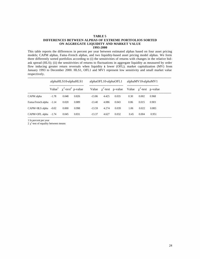
Unfortunately, when we follow the same testing strategy, our results are dramatically

different as reported in Table 5. We employ four alternative pricing models. The traditional

CAPM, the three-factor Fama-French model, and the two CAPM liquidity-based models

discussed in this paper in which we add the liquidity factor (either HLS or OFL) to the

usual CAPM model. We report the differences in alphas between January 1993 and

December 2000 on an annual basis. None of the models seems to indicate that there exists a

liquidity premium. In fact, regardless of which model is considered, we do not find

significant differences for HLS and size-sorted portfolios. This suggests that there was

neither a liquidity nor a size-related premium in the Spanish market in the nineties. It is

relevant to point out tha t adding the OFL factor to the CAPM does not seem to have any

effect on the results. For examples the differences in alphas between portfolios HLS10 and

HLS1 is –1.78 for the CAPM, and –1.74 for the CAPM once the OFL factor has been

added to the model. The liquidity-based CAPM when we use our HLS systematic liquidity

factor has a stronger impact on the result. The alpha is now just –0.02. In any case, as

observed above, none of the differences is significantly different from zero. However, the

striking result is the negative and significant difference between the alphas of the extreme

portfolios when we use the ranking based on the OFL factor. This is consistent with the

result already reported in Table 3. Stocks very highly sensitive to the OFL factor tend to

strongly underperform stocks with low sensitivity to the OFL factor. Of course, this is very

disturbing evidence for the liquidity-based model proposed by P&S.

14 The three Fama -French factor plus a momentum factor. In any case, regardless of which model is used, they

13

4.2 Cross-Sectional Evidence

We now perform empirical tests for both the conditional and unconditional liquidity-based

asset pricing models using the two systematic factors described in the paper.

A. General Asset Pricing Framework

The fundamental equation of asset pricing is usually written as:

( )[ ]E M R Nt t jt− + = =1 1 1 1 ; j ,..., (7)

where M t is the stochastic discount factor. Let mtR be the return on the true mean-variance

efficient portfolio. Then, we know that the discount factor under the liquidity-based

unconditional pricing model is given by:

t2mt10t LRM δδδ ++= (8)

where δ0 , δ1 and 2δ are three constants, and tL is the replicating liquidity portfolio as

given by either HLS or OFL. On the other hand, the conditional version may be written as,

t1t2mt1t11t0t LRM −−− ++= δδδ (9)

where δ0 1t − , δ1 1t − and 1t2 −δ are now allowed to vary over time.

Given that the true conditional distribution is unobservable, we merely assume (as usual in

conditional asset pricing literature) a linear relationship between the parameters δ0 1t − ,

δ1 1t − , 1t2 −δ and a time t-1 information variable, Zt − 1 , where Zt − 1 is a predicting

variable for returns given by the (log) aggregate book-to-market ratio, 1tbm − :

0,1,2i ; bm 1t1ii1it =+= −− δδδ (10)

find a very similar evidence.

14

where iδ and 1iδ are constants. Plugging (10) into (9), we transform the conditional

liquidity-based asset pricing model into the so called scaled liquidity-based asset pricing

model15, which is simply an unconditional multifactor model with constant coefficients.

The fundamental asset pricing equation is then,

( ) ( )[ ]( ){ } 1R1LbmLRbmRbmE jtt1t21t2mt1t11mt11t0101t =++++++ −−−− δδδδδδ (11)

The corresponding beta coefficients are given by

( )

( )mt

mtjtjm Rvar

R,Rcov=β (12)

( )

( )1t

1tjtjbm bmvar

bm,Rcov

−

−=β (13)

( )

( )mt1t

mt1tjtjmbm Rbmvar

Rbm,Rcov

−

−=β (14)

( )

( )t

tjtjL Lvar

L,Rcov=β (15)

( )

( )t1t

t1tjtjLbm Lbmvar

Lbm,Rcov

−

−=β (16)

The asset pricing model (11) can be written in the traditional multi-beta representation as:

( ) jLbm)7(5jL)6(4jmbm3jbm2jm10jRE βγβγβγβγβγγ +++++= (17)

15

where 4γ and 5γ correspond to HLS, and 6γ and 7γ to OFL. This will be the basic model

employed in our empirical exercise to test the competing liquidity-based pricing models.

B. Empirical Evidence

The results are reported for three alternative set of portfolios. In particular, as the dependent

variable in the Fama-MacBeth monthly regressions, we employ the 10 portfolios

constructed on the basis of sensitivity to liquidity and the traditional 10 size-sorted

portfolios. The results are quite similar independently of the endogenous variable used in

the test. As expected, the liquidity premium associated with the HLS factor is always

positive but, unfortunately, it is never significantly different from zero. The results relative

to the OFL factor are even more disappointing because, except for the size-sorted

portfolios, the liquidity premium has the wrong sign. This is consistent with the differences

in alphas found in Table 5.

It seems possible to conc lude that in the Spanish market, at least in the nineties, there was

not a significant liquidity premium. From our point of view, it may be important to further

analyze the potential interpretations that current research gives to the systematic liquidity

factor. It seems reasonable to expect more theory to be developed before making

conclusions on a particular liquidity-based market-wide factor. None of the factors

analyzed in this paper seems to be priced in the Spanish market, despite the success of the

P&S factor when US market data is employed. Of course, the results should be interpreted

with care given the short period of time covered by this research. Unfortunately, the

Spanish continuous market did not start trading until 1989. Given the design employed in

any asset pricing work, where key parameters are estimated with relatively long series of

past data, we are forced to use monthly data only from 1993 to 2000 in our tests of the asset

pricing models. This may be considered to be short for a paper of these characteristics. On

other hand, testing a model like the one proposed by P&S with an alternative database and

making comparisons with competing liquidity factors seems to be a crucial step in this type

of research.

15 See Cochrane (2001).

16

There are, however, other interesting results in Table 6. When the OFL portfolios are used,

the market risk premium becomes positive and significant. Although not reported, the

estimate of the market premium in the traditional CAPM context is 1.10 with a t-value of

0.13. This implies a tremendous amount of noise in the estimated coefficient. When the

HLS factor is added, the market risk premium becomes large and significant. Moreover,

under the HLS portfolios, the t-statistic associated with the estimated market risk premium

becomes 1.40 when the betas with respect to the HLS factor are employed in the cross-

sectional regressions.

Finally, in terms of the conditional version of the models and for the HLS factor, both the

market risk premium and the liquidity premium have the correct positive sign, but we can

never statistically reject their being zero. The liquidity premium, in all cases, becomes

much larger in magnitude than the one obtained under the unconditional version. However,

they are all estimated with too much noise and, consequently, the liquidity premium is

never significantly different from zero. Interestingly, the coefficient associated with the

instrument is always negative and highly significant. The book-to-market ratio predicts

returns in a positive fashion. Moreover, any increase in BM suggests that market prices go

down relatively more than book values. This fall represents bad news for the market.

Hence, assets whose returns co-vary positively with the (lagged) BM ratio tend to pay when

marginal utility is high (financial wealth low), and therefore investors should be “willing”

to pay to invest in those stocks. This explains the negative sign of the BM beta, and it

points toward a relevant state variable in asset pricing. It should be recalled that the BM

ratio plays a similar role to the consumption-wealth ratio of Lettau and Ludvigson in the

US market16.

16 See Nieto and Rodríguez (2002).

17

5. Conclusions

Market-wide liquidity should be a key ingredient of asset pricing models. If

macroeconomic variables anticipate economic recessions, they may also anticipate lower

aggregate liquidity. Indeed, the surprising success of the Fama-French HML risk factor

may be explained by a state variable closely related to systematic liquidity. The HML

factor is usually associated with a distress factor not theoretically identified. Taking into

account that risky assets compensate not only beta risk but also the fact that they have a

particularly poor performance in recession, it seems plausible to think of systematic

liquidity as the missing factor. Unfortunately, none of the market-wide liquidity factors

analyzed in this paper seems to be priced in the Spanish market. Thus, in our database,

expected stock returns are not related cross-sectionally to betas of returns to innovations in

aggregate liquidity. It seems to be the case that stocks that are more sensitive to systematic

liquidity do not have statistically higher expected returns either conditionally or

unconditionally. However, a predicting state variable such as the book-to-market ratio plays

a relevant role in explaining average returns in Spain.

18

REFERENCES

Acharya, V., and L. Pedersen (2002). “Asset Pricing with Liquidity Risk”, Working Paper,

London Business School.

Amihud, Y., and H. Mendelson (1986). “Asset Pricing and the Bid-Ask Spread”, Journal of

Financial Economics 17, 223-249.

Brennan, M,. and M. Subrahmanyam (1996). “Market Microstructure and Asset Pricing:

On the Compensation for Illiquidity in Stock Returns”, Journal of Financial Economics 41,

441-464.

Campbell, J. (2001). “Asset pricing at the Millennium”, Journal of Finance 55, 1515-1567.

Campbell, J., Grossman, S., and J. Wang (1993). “Trading Volume and Serial Correlation

in Stock Returns”, Quarterly Journal of Economics 108, 905-939.

Chordia, T, Roll, R., and A. Subrahamanyam (2000), “Commonality in Liquidity”, Journal

of Financial Economics 56, 3-28.

Chordia, T, Roll, R., and A. Subrahamanyam (2002), “Order Imbalance, Liquidity, and

Market Returns”, Journal of Financial Economics 65, 111-130.

Cochrane, J. (2001). “Asset Pricing”, Princeton University Press, Princeton, NJ.

Constantinides, G. (2002). “Rational Asset Prices”, Journal of Finance 57, 1567-1591.

Domowitz, I., and X. Wang (2002). “Liquidity, Liquidity Commonality and Its Impact on

Portfolio Theory”, Working Paper, Penn State University.

19

Easley, D., Hvidkjaer, S., and M. O´Hara (2002). “Is Information Risk a Determinants of

Asset Returns?, forthcoming in the Journal of Finance.

Ericsson, J., and O. Renault (2000). “Liquidity and Credit Risk”, Working Paper, McGill

University, Montreal.

Hasbrouck, J., and D. Seppi (2001). “Common Factors in Prices, Order Flows, and

Liquidity”, Journal of Financial Economics 59, 383-411.

Holmström, B., and J. Tirole (2001). “LAPM: A Liquidity-Based Asset Pricing”, Journal of

Finance 56, 1837-1867.

Lettau, M, and S. Ludvigson (2001). “Consumption, Aggregate Wealth, and Expected

Stock Returns, Journal of Finance 56, 815-849.

Lustig, H. (2001). “The Market Price of Aggregate Risk and the Wealth Distribution”,

Working Paper, Stanford University.

Nieto, B. (2002). “La Valoración Intertemporal de Activos: Un Análisis Empírico para el

Mercado Español de Valores”, forthcoming in Investigaciones Económicas.

Nieto, B., and R. Rodríguez (2002). “Consumption-Wealth Ratio, Book-To-Market Ratio,

and Asset Pricing”, Working Paper, Universidad de Alicante, X Foro de Finanzas, Sevilla.

Pastor, L., and R. Stambaugh (2002). “Liquidity Risk and Expected Stock Returns”,

forthcoming in the Journal of Political Economy.

20

TABLE 1 MARKET-WIDE COMMONALITY IN LIQUIDITY (Relative Spread)

1991-2000 (average figures for 204 stocks)

jtmtjjjt DSPDSP εβα ++=

where DSPjt is the percentage change from month t-1 to t in liquidity as proxied by the relative spread of stock j, and DSPmt is the concurrent change in a cross-sectional average of the same variable or the market-wide (equally-weighted) relative spread ------------------------------------------------------------------------------------------------------------------------------ Avg. Alpha Avg. Beta Avg. R2 Avg. Adj R2 ------------------------------------------------------------------------------------------------------------------------------ Coefficient 0.0886 0.8815 0.1377 0.1091 (avg. t-stat) (1.031) (2.639) % Positive - 94.1 - - % + significant - 63.2 - - ------------------------------------------------------------------------------------------------------------------------------

21

TABLE 2 SUMMARY STATISTICS FOR RISK FACTORS

1993-2000 The numbers represent the average annualized average returns, volatilities, skewness, excess kurtosis and correlation coefficients of alternative risk factors employed in the paper. RM is the equally-weighted market portfolio, SMB is the Fama -French size related factor, HML is the Fama -French book-to-market related factor, HLS is the liquidity factors associated with sensitivities to the bid-ask spread, and OFL is the liquidity factor based on the order flow inducing greater return reversals when liquidity is lower. The figures are obtained from monthly returns from January 1993 to December 2000. ------------------------------------------------------------------------------------------------------------------------------------

PANEL A Risk Factor Average Return Volatility Skewness Excess Kurtosis ------------------------------------------------------------------------------------------------------------------------------------ RM 19.53 18.75 0.765 1.242 SMB -0.69 13.15 0.656 0.224 HML 1.48 11.00 0.493 0.140 HLS -0.04 12.38 -1.009 6.043 OFL -1.17 25.20 -1.389 4.122 ------------------------------------------------------------------------------------------------------------------------------------

PANEL B Correlation Coefficients

------------------------------------------------------------------------------------------------------------------------------------ RM SMB HML HSL OFL RM 1.000 0.066 -0.097 0.160 0.069 SMB 1.000 0.094 0.139 0.218 HML 1.000 -0.042 0.094 HLS 1.000 0.067 OFL 1.000 ------------------------------------------------------------------------------------------------------------------------------------

22

TABLE 3 SUMMARY STATISTICS FOR PORTFOLIOS

1993-2000 The summary statistics represent the time-series annualized averages of returns, volatilities, and factor betas of three differently sorted portfolios according to (i) the sensitivities of returns with changes in the relative bid-ask spread (HLS); (ii) the sensitivities of returns to fluctuations in aggregate liquidity as measured by order flow inducing greater return reversals when liquidity is lower (OFL); market capitalization (MV) from January 1993 to December 2000. HLS1, OFL1 and MV1 represent low sensitivity, and small market value respectively. ------------------------------------------------------------------------------------------------------------------------------------ Portfolios Average Return Volatility HLS Beta (t-stat) OFL Beta (t-stat) ------------------------------------------------------------------------------------------------------------------------------------ HLS1 20.84 26.43 -0.583 (-2.75) - HLS2 17.14 19.85 -0.074 (-0.45) - HLS3 19.68 16.74 -0.053 (-0.38) - HLS4 14.00 15.97 0.049 ( 0.40) - HLS5 17.23 19.19 0.117 ( 0.73) - HLS6 15.72 18.78 0.219 ( 1.41) - HLS7 21.62 19.94 0.376 ( 2.33) - HLS8 19.06 21.16 0.446 ( 2.56) - HLS9 16.62 21.07 0.606 ( 3.70) - HLS10 21.77 26.60 0.855 ( 4.21) - OFL1 27.13 25.07 - -0.067 (-1.45) OFL2 20.57 18.71 - -0.022 (-0.63) OFL3 17.00 19.60 - -0.011 (-0.31) OFL4 20.94 18.30 - 0.011 ( 0.33) OFL5 19.96 18.17 - 0.016 ( 0.47) OFL6 12.49 16.66 - 0.017 ( 0.57) OFL7 18.38 21.65 - 0.030 ( 0.73) OFL8 15.92 20.69 - 0.043 ( 1.12) OFL9 23.45 21.92 - 0.042 ( 1.03) OFL10 13.93 24.03 - 0.093 ( 2.12) MV1 26.59 33.48 0.092 (0.33) 0.023 (0.33) MV2 22.33 24.93 0.192 (0.93) 0.019 (0.41) MV3 12.81 21.11 0.299 (1.72) 0.002 (0.06) MV4 18.75 21.88 0.097 (0.53) 0.012 (0.28) MV5 20.45 18.69 0.231 (1.50) 0.033 (0.94) MV6 15.20 17.91 0.180 (1.21) 0.005 (0.14) MV7 17.59 16.64 0.146 (1.06) 0.019 (0.61) MV8 19.77 17.91 0.320 (2.20) 0.020 (0.59) MV9 20.30 18.46 0.362 (2.43) 0.034 (1.00) MV10 19.78 19.33 0.523 (3.45) 0.063 (1.78) ------------------------------------------------------------------------------------------------------------------------------------

23

TABLE 4

MARKET-WIDE COMMONALITY IN LIQUIDITY (Relative Spread) PORTFOLIOS BY AGGREGATE LIQUIDITY AND MARKET VALUE

1993-2000

jtmtjjjt DSPDSP εβα ++=

where DSPjt is the percentage change from month t-1 to t in liquidity as proxied by the relative spread of portfolio j, and DSPmt is the concurrent change in a cross-sectional average of the same variable or the market-wide (equally-weighted) relative spread. This table reports results from three differently sorted portfolios according to (i) the sensitivities of returns with changes in the relative bid-ask spread (HLS); (ii) the sensitivities of returns to fluctuations in aggregate liquidity as measured by order flow inducing greater return reversals when liquidity is lower (OFL); market capitalization (MV) from January 1993 to December 2000. HLS1, OFL1 and MV1 represent low sensitivity and small market value respectively. ------------------------------------------------------------------------------------------------------------------------------------ Portfolios Slope Coefficient t -statistic Adjusted R2

------------------------------------------------------------------------------------------------------------------------------------ HLS1 1.899 (7.30) 0.357 HLS2 1.434 (1.98) 0.090 HLS3 1.004 (4.45) 0.167 HLS4 1.620 (5.11) 0.211 HLS5 1.489 (4.04) 0.140 HLS6 0.839 (2.38) 0.047 HLS7 0.552 (1.21) 0.050 HLS8 0.669 (4.20) 0.150 HLS9 0.328 (1.98) 0.030 HLS10 0.530 (5.59) 0.243 OFL1 0.879 (3.99) 0.137 OFL2 1.034 (5.98) 0.270 OFL3 1.296 (4.71) 0.184 OFL4 1.349 (3.50) 0.107 OFL5 0.660 (2.25) 0.042 OFL6 0.736 (1.98) 0.030 OFL7 0.744 (3.56) 0.120 OFL8 0.434 (2.10) 0.035 OFL9 0.929 (4.65) 0.180 OFL10 0.765 (5.00) 0.203 MV1 1.266 (5.61) 0.245 MV2 1.001 (5.55) 0.241 MV3 0.915 (3.15) 0.087 MV4 1.401 (3.62) 0.114 MV5 1.119 (6.22) 0.286 MV6 0.896 (5.54) 0.240 MV7 1.269 (6.33) 0.294 MV8 0.595 (7.65) 0.379 MV9 0.235 (2.30) 0.044 MV10 0.100 (5.52) 0.239 ------------------------------------------------------------------------------------------------------------------------------------

24

TABLE 5 DIFFERENCES BETWEEN ALPHAS OF EXTREME PORTFOLIOS SORTED

ON AGGREGATE LIQUIDITY AND MARKET VALUE 1993-2000

This table reports the differences in percent per year between estimated alphas based on four asset pricing models; CAPM alphas, Fama -French alphas, and two liquidity-based asset pricing model alphas. We form three differently sorted portfolios according to (i) the sensitivities of returns with changes in the relative bid-ask spread (HLS); (ii) the sensitivities of returns to fluctuations in aggregate liquidity as measured by order flow inducing greater return reversals when liquidity is lower (OFL); market capitalization (MV) from January 1993 to December 2000. HLS1, OFL1 and MV1 represent low sensitivity and small market value respectively. ------------------------------------------------------------------------------------------------------------------------------------ alphaHLS10-alphaHLS1 alphaOFL10-alphaOFL1 alphaMV10-alphaMV1 ------------------------------- ------------------------------- ----------------------------- Value1 χ2-test2 p-value Value χ2-test p-value Value χ2-test p-value ------------------------------------------------------------------------------------------------------------------------------------ CAPM alpha -1.78 0.048 0.826 -13.86 4.425 0.035 0.30 0.002 0.968 Fama-French alpha -1.14 0.020 0.889 -13.40 4.086 0.043 0.86 0.015 0.903 CAPM+HLS alpha -0.02 0.000 0.998 -13.59 4.274 0.039 1.06 0.022 0.883 CAPM+OFL alpha -1.74 0.045 0.831 -13.37 4.627 0.032 0.45 0.004 0.951 --------------------------------------------------------------------------------------------------------------------------------------------------------------------- 1 In percent per year 2 χ2-test of equality between means

25

TABLE 6 CROSS-SECTIONAL UNCONDITIONAL AND CONDITIONAL ASSET PRICING MODEL TESTS

1993-2000 This table contains the time series averages of the monthly coefficients in cross-sectional asset pricing tests using standard Fama-MacBeth methodology. The dependent variable is the monthly return on three differently sorted portfolios according to (i) the sensitivities of returns with changes in the relative bid -ask spread (HLS); (ii) the sensitivities of returns to fluctuations in aggregate liquidity as measured by order flow inducing greater return reversals when liquidity is lower (OFL); market capitalization (MV) from January 1993 to December 2000. The explanatory variables are the betas of the different factors estimated (when possible) with the 35 previous monthly returns to each cross-sectional estimation and the corresponding month itself for a total of 36 observations in each regression. The conditioning variable is the (log) of the aggregate book-to-market ratio, and the models are the standard CAPM and two liquidity-based asset pricing models. The cross-sectional regressions for each month take the following form:

jjOFLbm7jOFL6jHLSbm5jHLS4jmbm3jbm2jm10jR ηβγβγβγβγβγβγβγγ ++++++++=

------------------------------------------------------------------------------------------------------------------------------------ PANEL A: 10 HLS PORTFOLIOS

------------------------------------------------------------------------------------------------------------------------------------ γ0 γ1 γ2 γ3 γ4 γ5 γ6 γ7 R

2 ------------------------------------------------------------------------------------------------------------------------------------

0.2288 1.0775 - - 0.0448 - - - 41.9 (0.42) (1.40) (0.12) 0.1607 1.1705 - - - - -5.258 - 33.4 (0.24) (1.30) (-1.40) 1.2778 0.1881 -22.160 -0.3063 0.5895 0.1904 - - 71.1 (2.02) (0.22) (-3.44) (-0.79) (1.11) (0.62) 1.0058 0.3353 -12.567 -0.2141 - - -5.5506 1.0186 69.7 (1.65) (0.38) (-2.25) (-0.55) (-1.14) (0.78)

------------------------------------------------------------------------------------------------------------------------------------ PANEL B: 10 OFL PORTFOLIOS

------------------------------------------------------------------------------------------------------------------------------------ γ0 γ1 γ2 γ3 γ4 γ5 γ6 γ7 R

2 ------------------------------------------------------------------------------------------------------------------------------------

-0.8835 2.2450 - - 0.2773 - - - 31.9 (-1.18) (2.21) (0.38) -0.2216 1.5790 - - - - -0.8743 - 32.5 (-0.33) (1.91) (-0.40) -0.1617 1.5408 -18.444 0.0583 0.6452 0.2385 - - 69.3 (-0.16) (1.32) (-3.55) (0.17) (0.71) (0.70) 0.9389 0.4688 -12.302 -0.2190 - - -1.1319 -0.1218 70.3 (1.05) (0.46) (-2.45) (-0.51) (-0.50) (-0.15)

------------------------------------------------------------------------------------------------------------------------------------ PANEL C: 10 MV PORTFOLIOS

------------------------------------------------------------------------------------------------------------------------------------ γ0 γ1 γ2 γ3 γ4 γ5 γ6 γ7 R

2 ------------------------------------------------------------------------------------------------------------------------------------

0.5347 0.8529 - - 0.4998 - - - 43.7 (0.87) (1.08) (0.79) 0.9540 0.4447 - - - - 1.1727 - 40.7 (1.59) (0.59) (0.42) 1.3824 -0.0674 -16.334 -0.324 0.7414 0.1561 - - 75.8 (2.08) (-0.07) (-3.13) (-0.99) (0.95) (0.59) 1.4940 -0.1376 -20.645 -0.409 - - 3.4146 0.1715 72.7 (2.53) (-0.15) (-3.21) (-1.06) (0.98) (0.19)

---------------------------------------------------------------------------------------------------------------------------------------------------------------------