Assessment on Traffic Operations Performance Measures and Data Collection/Dissemination Plan for...

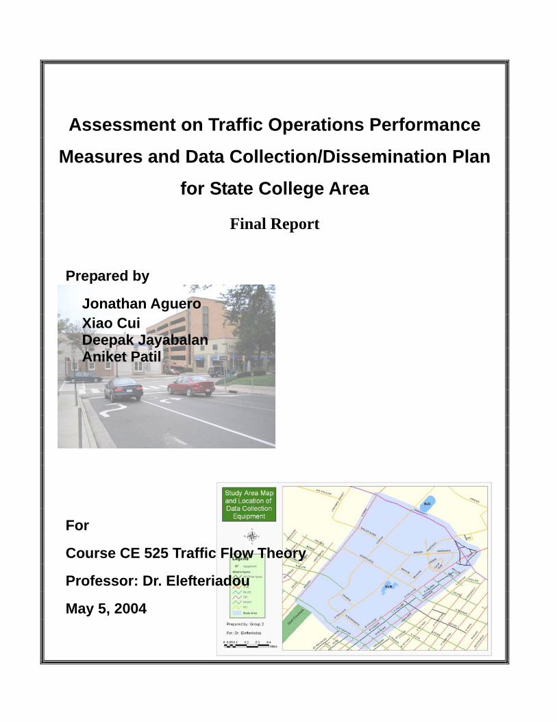
Assessment on Traffic Operations Performance

Measures and Data Collection/Dissemination Plan

for State College Area

Final Report

Prepared by

Jonathan Aguero Xiao Cui Deepak Jayabalan Aniket Patil

For

Course CE 525 Traffic Flow Theory

Professor: Dr. Elefteriadou

May 5, 2004

Aguero, Cui, Jayabalan and Patil i

Table of Contents

1. Introduction..................................................................................................................... 1

2. Performance Measures.................................................................................................... 1

2.1 Travel Time............................................................................................................... 1

2.2 Density ...................................................................................................................... 2

2.3 Speed......................................................................................................................... 3

2.4 Incident/Congestion .................................................................................................. 3

3. Equipment and Data Collection ...................................................................................... 4

3.1 Loops......................................................................................................................... 4

3.2 Infrared, Radar Technology ...................................................................................... 5

3.3 Probe Vehicles .......................................................................................................... 5

3.4 CCTV and Video Image Detection System.............................................................. 5

4. Data Quality .................................................................................................................... 6

5. Communication............................................................................................................... 6

5.1 Traffic Management Center...................................................................................... 7

5.2 Dynamic Message Signs ........................................................................................... 7

6. Assessment on Required Performance Measures and Data Collection/Dissemination Plan ..................................................................................................................................... 7

6.1 Determine Current Data Availability........................................................................ 7

6.2 Assess Information Needs......................................................................................... 9

6.2.1 Location of Data Collection Points........................................................................ 9

6.2.2 Equipment Selection .......................................................................................... 9

6.2.3 User Information Requirements....................................................................... 11

6.2.4 System Operator Information requirements..................................................... 11

6.3 Utilization of the Available Data ............................................................................ 12

Aguero, Cui, Jayabalan and Patil ii

6.4 Determine Best Information Delivery Mechanism................................................. 15

6.5 Install, Test, and Operate the Infrastructure............................................................ 17

7. Conclusion .................................................................................................................... 17

8. References..................................................................................................................... 18

List of Figures, Tables, and Maps

Figure 1 Ratings on Type of Traffic Information.. ........................................................... 11

Figure 2 Example of Traffic Conditions Map for State College. ..................................... 16

Table 1 Data sources for various data needs....................................................................... 9

Table 2 Quantitative Evaluation of Detectors at Signalized Intersections… ... ...……….10

Table 3 Color code for the flow density map according to occupancy values ................. 14

Table 4 Color code for the flow density map according to degree of congestion ............ 14

Map 1 Study Area Map and Location of Data Collection Points ....................................... 8

Aguero, Cui, Jayabalan and Patil 1

1. Introduction

The objectives of the traffic performance monitoring plan are to evaluate traffic operations continuously and to provide real-time traveler information. Therefore the performance measures selected must be identified in response to these goals and objectives. The performance measures frequently identified are travel time, variance in the travel time, speed, delay, volume, safety, vehicle emissions, congestion extent and duration, and average vehicle occupancies. These performance measures can influence the decisions of travelers as well as system operators, planners, facility designers, program developers and politicians. It is important to note that estimated travel time is one of the most important parameters that are of concern to the traveler.

The aim of the project is to develop a data collection, processing, analysis, and dissemination plan for the downtown State College area. A detailed literature review on some of the state-of-the-art practices in traffic monitoring and control is presented along with recommendations for a traffic monitoring plan for the State College area. The report is divided into two parts. The first part contains the literature review and the latter part contains the recommendations of the group for the traffic monitoring plan.

2. Performance Measures

As mentioned earlier some of the performance measures identified include travel time, variance in the travel time, speed, delay, volume, safety, vehicle emissions, congestion extent and duration, and average vehicle occupancies. Findings in literature on some of the critical performance measures and equipments available for obtaining them are discussed in the following paragraphs.

2.1 Travel Time

Travel time is one of the most important performance measures, if not the most, because it is used by the operators, planners, and designers and more importantly by the travelers. The emphasis on new technology to measure travel time is partially due to a misunderstanding of how to interpret vehicle travel times. For example, the average velocity sampled at a detector station over fixed time periods as a base case in the analysis (1). The authors found that link travel times differed significantly from the quotient of local velocity and the link distance. But this result is not surprising, since the link travel time for a vehicle reflects traffic conditions averaged over a fixed distance and a variable amount of time, while the detector data only reflects traffic conditions averaged over a fixed time period at a single point in space.


One of the most advanced Traffic Information and Monitoring Systems in the United States is the one implemented by the Washington Sate Department of Transportation (WSDOT) in the Puget Sound region (including Seattle)(2). The WSDOT is using operational data to monitor and measure system performance, especially speed and travel time derived from loop detectors on urban freeways. These measurements are received on real-time and communicated to the users through the web page of the department.

One of the interesting research areas in travel time estimation is vehicle tracking or reidentification. A vehicle’s movement is tracked through the traffic facility system identifying its location and arrival time, so that travel times can be collected (3). One of the latest advances in this area is the use of inductive signatures from loops with high speed scanning detector cards to reidentify vehicles passing over a second loop and to calculate space mean speed and travel time (4). The reidentification rate is small (42%) but for the vehicles identified at second loop, the travel time derived was within 10% error.

Current technologies like GPS and Cellular phones are increasingly used for vehicle tracking to measure travel time. However to equip a sufficient number of vehicles for obtaining a statistically representative sample size could be very expensive for some Traffic Management Centers. A key issue in probe-based monitoring is determining the minimal number of probes to sample to assure acceptable data quality.

A recent work addresses this issue by using the Central Limit Theorem Method (5) to reduce the sample size while still maintaining the desired confidence and accuracy levels. An alternative approach on travel time estimation is the use of platoons or groups of vehicles instead of tracking or reidentifying a single vehicle. This method will use the existent loop infrastructure by identifying the wave of the platoon from information collected each second. The method provides relatively good travel time measures for arterial networks with a low cost.

An innovative method for estimating travel time is using bus travel time data in urban corridors (6). In this work, the authors measured travel times for transit and normal vehicles simultaneously. The analysis reveals that the difference in travel times was relatively stable, and consequently, appropriate formulas for predicting the travel time of the automobile were developed.

2.2 Density

Density is a spatial measure taken in a determinate moment, a picture of the road at a given time. This characteristic makes density a very difficult variable to measure. In recent years remote sensing is been used to overcome this problem. One can easily measure flow (q) and velocity (v) at a point in space with conventional traffic detectors, but density (k) is more difficult to measure. Hence it can only be estimated. Density can be calculated based on field measurements of speed and flow. Another technique for determining density is based on measurement of occupancy. Mathematically density can be found if average vehicle length and detection zone length is known. Density may be calculated utilizing the vehicles reidentification techniques. In addition to the previously mentioned vehicles


signature approach there are two popular methods in matching vehicles (7). One is identifying a sequence of vehicle lengths and the other is identifying a unique vehicle depending on its length. Although an individual length measurement is not unique, a sequence of measurements rapidly becomes identifiable and this first algorithm uses the sequence of length measurements at each station to match platoons of vehicles that pass both detector stations. Unfortunately, the dual loop detector measurement resolution degrades as vehicle speed increases. At free flow speeds most cars become indistinguishable from one another, but because of the large range of feasible lengths, it is still possible to distinguish between the long vehicles at these speeds. So the second algorithm only attempts to match the long vehicles during free flow conditions. These are under the assumption that there are few detector errors and lane changing is minimal. Distance between the two detectors is known, the travel time of the vehicles is known, and flow rate is known. Hence density can be estimated as follows

ceTraveledDisFlowRateTravelTimeDensity

tan×

=

The photographic technique is a recent one. It uses pictures taken from an aircraft-mounted camera to measure density. A series of pictures is taken along the roadway and vehicles are identified from the images. Before the vehicles are detected some correction procedures like Lens distortion correction, Ortho-Rectification, Radiometric correction are done on the images to enhance them. Length of study area is pre-decided based on speed of the aircraft and the time interval between sets of photographs (8) (7).

The availability of high resolution satellite images commercially, has promoted the application of Remote Sensing in Transportation Engineering. They are being increasingly used in determining traffic performance measures like density. Despite the recent developments in this field, better vehicle detection/classification algorithms are in demand to increase the correct vehicle detection ratio (9).

2.3 Speed

Speed is another important performance measure especially on highways. As mentioned before point speeds and flows are often used to calculate densities, which are the performance measure for highways establish by the Highway Capacity Manual (HCM) (10). Moreover, speed is still used as performance measure for other transportation facilities like urban streets and two-lane highways. Now a days speed is perhaps the easiest parameter to measure if the field, with sensors that range from microwave detectors to double loops and video cameras.

2.4 Incident/Congestion

One of the essential functions of a traffic surveillance system is to determine reliably whether the facility is free flowing or congested. The capability to respond rapidly when the facility becomes congested is also critical. It is important to note that incident is a


qualitative estimate and hence cannot be measured. However it is possible to quantitatively define congestion. The term degree of congestion (r) is defined as the ratio of the current travel time to the free flow travel time.

These functions are complicated by the fact that conventional vehicle detectors are capable of only monitoring discrete points along the roadway while incidents may occur at any location on the facility. The point detectors are typically placed at least one-third of a mile apart and conditions between the detectors must be inferred from the local measurements. Two signals emanate from an incident, a backward moving shock wave and a forward moving drop in flow (11). It is difficult to identify an incident based strictly on changes in point measurements associated with the forward moving wave. Reliable detection of an incident using point measurements can happen only when both of the signals have been received at the detector stations. Although the drop in flow travels at the prevailing traffic velocity, Daganzo (12) estimated the shock wave velocity to be on the order of 8 mph. Fortunately, the drop in flow in the downstream detector data reflects the fact that vehicles are being delayed behind the incident and vehicle link travel time will increase after the signal has passed. So rather than waiting for the slow moving shock wave, the new algorithm could be used to quickly and reliably identify the onset of delay corresponding to the drop in flow.

Incident detection has proved to be critical for traffic system operations. On the traffic operator side, an early detection of an accident helps to reestablish the normal operation quicker and on the user side, commuters have the option of changing their route if they are aware of the incident. A recent research introduces the use of processed audio signal for detecting traffic incidents at intersections (13). The audio signal is classified as “crash” and “non-crash” with feature extraction statistical methods. A real word testing was conducted and accident detection accuracies of 95% to 100% with low false alarm rate.

3. Equipment and Data Collection

As documented in Ohio’s best ITS Practice Report (14), traffic detection uses devices, such as loop detectors and surveillance cameras, to monitor the traffic conditions and collect volume and speed data on the network. Detectors can provide traffic data for real-time and future analysis. The technology is changing rapidly.

3.1 Loops

The loops are by far the most utilized sensors in traffic data collection. They sense when a car passes by them and are capable of providing information on vehicle counts, speeds, and occupancies. The loop detects changes in the electromagnetic field (inductance) produced by the metallic body of the cars. Loop detectors are reliable but the major shortcoming is that they are not easy to repair. Also, installation expense is high. The device is known to fail due to improper sealing and because of deteriorating pavements. There are two categories of loop detectors, one is the single loop and the other is the dual loop (15).


Single loop detectors are capable of measuring flow and occupancy whereas the dual loop detectors can measure velocity in addition to the other two. It uses a speed trap technique to measure velocity. The speed trap detection system is redundant. Each vehicle is observed twice under normal operating conditions, once at each loop. The two observations are normally used to measure velocity.

A new variety of loops called “Blade sensors” has been used for vehicle inductive signature collection. These sensors provide key advantages over the standard loops. They are narrow (approximately 6 in wide) compared to the traditional loops (6 ft x 6 ft) and are capable of collecting more detailed inductive signatures which produces higher vehicle reidentification rates.

3.2 Infrared, Radar Technology

Non-inductive loop technologies, such as infrared or radar sensor, are being widely considered for use to overcome the shortcomings of the old loop technology. In the report of the Texas Transportation Institute (TTI) (16), several non-inductive systems are selected as they promise higher accuracy and reduced costs. Some of these systems include Autoscope Solo Pro, Iteris Vantage, RTMS by EIS, SAS-1 by SmarTek, Traficon NV, and 3M Microloops (17).

3.3 Probe Vehicles

The notion of "probe vehicles" measuring point-to-point travel times is gaining popularity. However, there are two different schemes for probe vehicles, "vehicle-centric" and "infrastructure-centric." The former uses an in-vehicle GPS to get the vehicle's location, while the latter uses sensors along the roadway (a la TRANSCOM's TRANSMIT program) to determine the vehicle’s location.

3.4 CCTV and Video Image Detection System

Surveillance cameras are critical for real-time monitoring. The images from the cameras are monitored by the traffic management staff and are used to trigger managing functions, such as changing the information on a Dynamic Message Sign (1). However, a report prepared by Texas Transportation Institute indicates that the cameras are difficult to mount and are easily affected by the present lighting conditions, shadows of other vehicles and bad weather. It is more suitable for spot check purpose (16).

Video Image Detection System is a modern technique of image processing and detection which is based on detecting deviation in brightness for extracting the vehicle’s spatial outline feature, which can be used for tracking it. Another method is based on the creation of virtual loop. In the virtual loop area the collected images of the road segment are compared with the background image of the same road segment. Based on this comparison the system determines the presence and speed of the vehicle.


4. Data Quality

The desirable aspects of data quality include accuracy, reliability and absence of bias. Checking for possible errors in data is a critical part of data management. Most agencies use some type of basic error checking procedure that identifies physically impossible or implausible data values, such as average 5-minute speeds greater than 80 mph or total 5-minute lane vehicle counts greater than 250. This error checking is performed at either the detector controller level or at the central database/archiving level. Most agencies will set data errors to special codes (e.g., “-1” or “255”), but few provide information or codes as to why the data was considered erroneous and dropped. A few agencies use more sophisticated error checking procedure, such as checking for implausible combinations of data values. A good instance is a combination of an occupancy value less than 5 percent but speed less than 20 mph.

5. Communication

Communication is essentially in two ways. Data must be collected using loops, sensors etc and communicated to the Traffic Management Centers (TMC), where they are processed. The processed data must be converted into a format that is decipherable by the user. In this case, the user is the traveler. Communication is a crucial component of the traffic performance measure system and has a large impact on both costs and performance of the system throughout its lifetime. The appropriate technology to use for communicating traffic data will depend on factors such as volume and nature of data, distances between where the data are collected and processed, communication services available in the area, and their cost. Either Wire line or Wireless solutions or a combination of both may comprise the communication system. Wire line technologies include twisted pair copper, Coaxial cable, Fiber optic (multimode and single mode). Wireless technologies include Microwave, Cellular (digital and analog), Cellular digital packet data (CDPD), Spread spectrum, Digital and trunked radio systems.

Fiber optic communications are the fastest and the most reliable option, but installation costs are high. Wireless communications have much lower installation costs but are slower. Leased telephone lines have been a common medium, but agencies must make sure that the carrier is providing reliable service. Increasingly, agencies are shifting to radio modems, which are generally less expensive than leased telephone lines. Most agencies use a combination of communications media. For example, Virginia DOT uses coaxial cable inside the beltway around Washington DC and fiber optic outside the beltway. The other components of the communication system namely the Traffic Management Center and the Dynamic Message Signs are explained briefly.


5.1 Traffic Management Center

Given the speed of internet, it is possible to put the live image on the web to inform drivers about the current traffic conditions (17).Traffic control is important to the real-time traffic management. In case of incident, traffic control, fire or police can coordinate to easy traffic jams and provide quickest path for needs. Usually, a Traffic Management Center is essential to perform the monitoring and coordinating job for traffic control. Traffic personnel are responsible for monitoring the live camera images and the data sent back from the detectors. Appropriate performance measures are determined and communicated to the users through available dissemination means (18).

5.2 Dynamic Message Signs

Dynamic Message Signs can inform commuters about traffic jam ahead of them in real-time. The text on the sign is controlled by the traffic management center. It can be used to inform drivers about accidents, weather or other information on the road.

6. Assessment on Required Performance Measures and Data Collection/Dissemination Plan

The main goal of the project is to develop a Traffic Performance Monitoring Plan for the State College Area. The System should provide data to address two main objectives: to evaluate traffic operations continuously and to provide real-time traveler information. Map 1 shows the Area of Study, the periphery of the Penn State main campus on State College, Pennsylvania. It can be seem that the area is an arterial network composed mainly by signalized and un-signalized intersections. The traffic monitoring setup process may be broadly divided into five tasks as mentioned below.

6.1 Determine Current Data Availability

The first step is to review the availability of installed surveillance equipment and the potential to easily install new surveillance equipment. Presently there are two traffic video cameras at the intersection of N. Atherton St. and Park Avenue capturing images of traffic flow on either direction. But these do not convey information about speed, flow rate and occupancy. They can be used only to visually examine traffic conditions.

Hence it is required that sensors and cameras be installed at critical locations of the downtown State College area. It is also required that these data be pooled into a central location, from where they may be analyzed. Data in this case include images from the camera and data from the detector including flow, speed and occupancy.

GolfCours

es

BJC

HUB

CURTIN

UNIVERSITY

EPA

RK

E COLLEGE

S PUGH

EFOSTER

E POLLOCK

E BEAVER

LOCUST

N ALLEN

EIR

VIN

S ALLEN

S GARNER

MCKEE

HASTINGS

WPARK

N ATHERTON

EPRO

SPECT

SHORTLIDGERID

GE

HETZEL

EHAM

ILTO

N

BIGLER

PORTER

ELMADAM

S

EFA

IRM

OUNT

WCALDER

WCOLLEGE

HOLMES

HIGH

CLAY

WARIN

G

WBEAVER

BIG HOLLOW

BIGLER ROAD

NBURROWES

EM

ITCHELL

MCKEAN

HARTSW

ICK ENTRANCE

SFRASER

MIFFLIN

ENIT

TANY

THOMAS

HIGHLAND

FRASER

BCRAILROAD

UN

NA

MED

STR

EET

LINDEN

KELLER

TULIP

E CALDER

RAMP

WNIT

TANY

MCCO

RMIC

K

N GILL

OAK

WFOSTER

FERG

USON

KELLER

HIGHLAND

E CALDER

Study Area Mapand Location ofData Collection

Equipment

0 0.1 0.2 0.30.05Miles

Prepared by: Group 2

For: Dr. Elefteriadou

Legend

equipment

streets types

All Other types

ST

AVE

BLVD

DR

PKWY

RD

Study Area


6.2 Assess Information Needs

The second step is to assess from which locations traffic condition information should be reported to meet the community’s traffic requirements. This step will target the data collection reporting efforts to the most critical and useful locations.

6.2.1 Location of Data Collection Points

The primary criteria are to minimize the number of cameras/detectors without compensating on the information requirements. Hence it is important that sensors be located at key intersections that tend to control or influence the performance of the network. The critical points would be the places that frequently experience congestion. Other areas to consider are arterial streets connecting the freeway ramps and arterial streets that serve as alternative routes to a freeway or other regional roadway.

The data collection points will be placed around the Penn State campus as shown in Map 1. It was felt there was rarely any congestion inside the campus, except on Burrows Road. Hence the sensors are densely located in the downtown area (6 in all) including the signalized intersection between Burrows Road and E College Avenue. Two data collection points are located on the University Drive and another one on the N. Atherton Street as shown in the figure. It was felt that intersection of University Drive and the Hastings Road rarely experienced congestion. The last data collection point is located on University Drive-College Avenue Intersection. Hence a total of ten data collection points are used for the area.

6.2.2 Equipment Selection

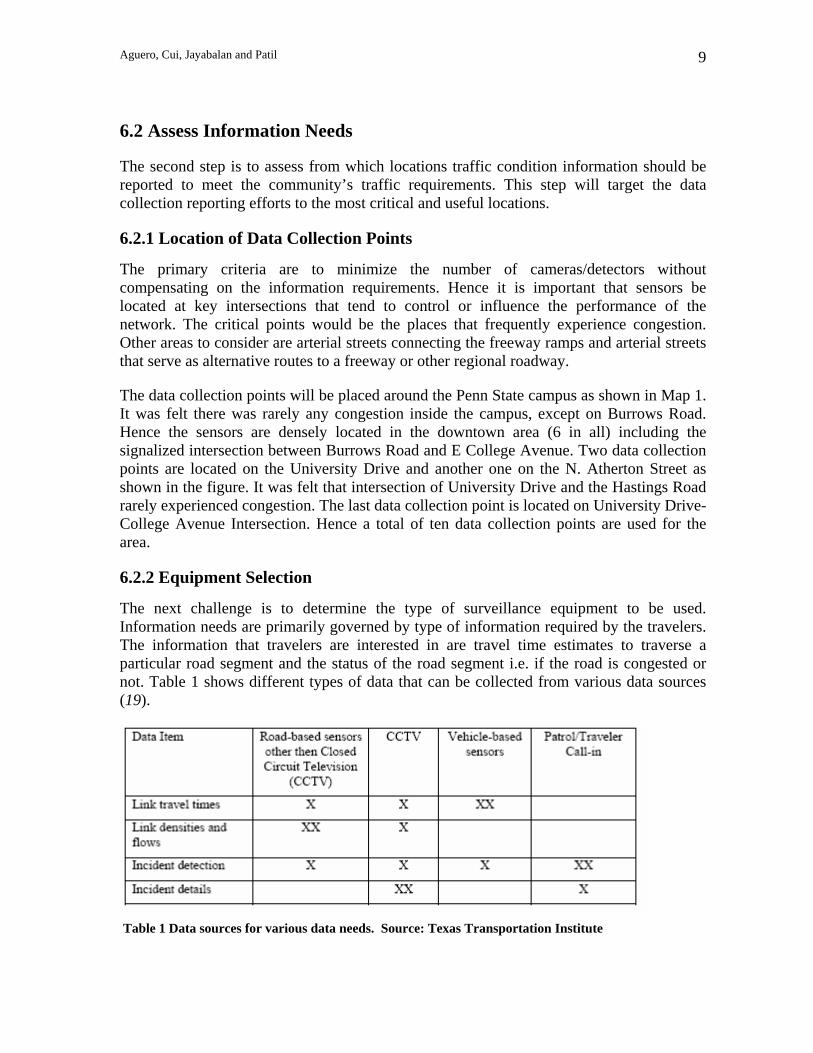
The next challenge is to determine the type of surveillance equipment to be used. Information needs are primarily governed by type of information required by the travelers. The information that travelers are interested in are travel time estimates to traverse a particular road segment and the status of the road segment i.e. if the road is congested or not. Table 1 shows different types of data that can be collected from various data sources (19).

Table 1 Data sources for various data needs. Source: Texas Transportation Institute


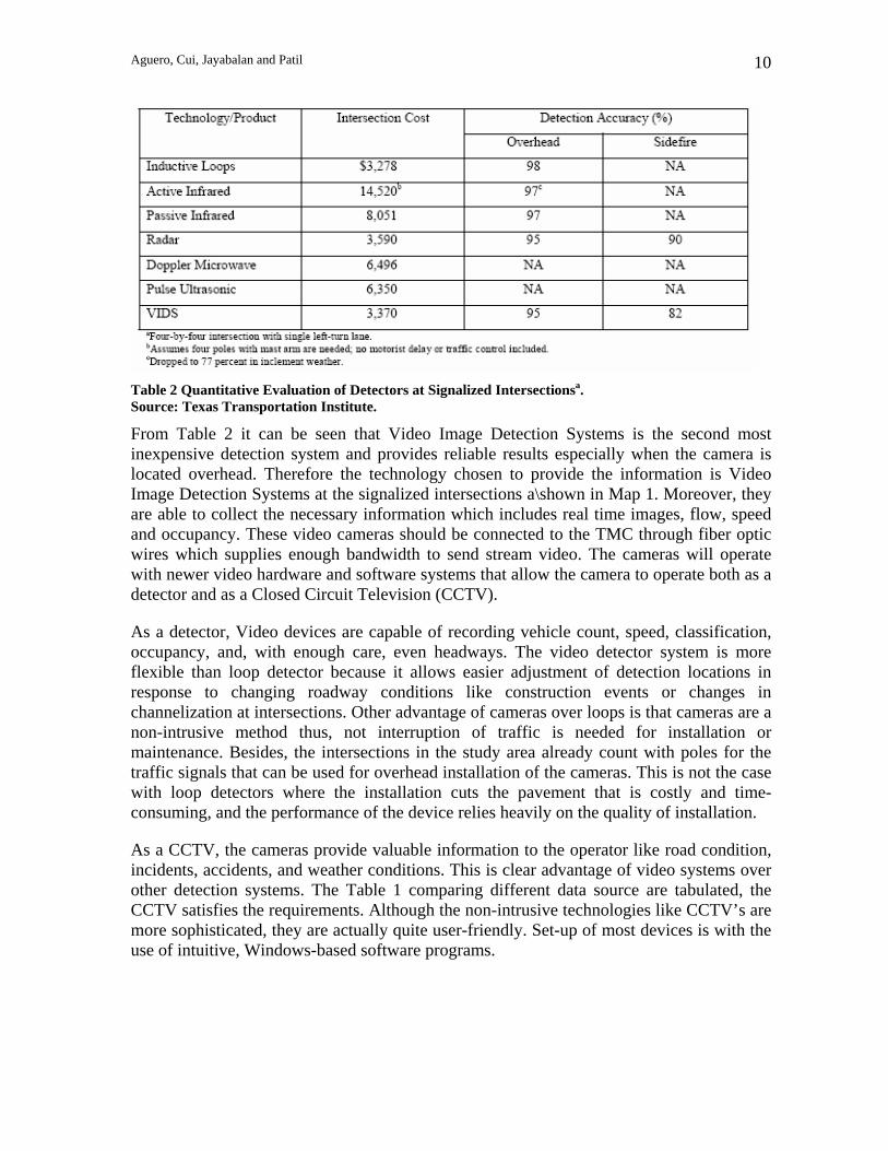
Table 2 Quantitative Evaluation of Detectors at Signalized Intersectionsa. Source: Texas Transportation Institute.

From Table 2 it can be seen that Video Image Detection Systems is the second most inexpensive detection system and provides reliable results especially when the camera is located overhead. Therefore the technology chosen to provide the information is Video Image Detection Systems at the signalized intersections a\shown in Map 1. Moreover, they are able to collect the necessary information which includes real time images, flow, speed and occupancy. These video cameras should be connected to the TMC through fiber optic wires which supplies enough bandwidth to send stream video. The cameras will operate with newer video hardware and software systems that allow the camera to operate both as a detector and as a Closed Circuit Television (CCTV).

As a detector, Video devices are capable of recording vehicle count, speed, classification, occupancy, and, with enough care, even headways. The video detector system is more flexible than loop detector because it allows easier adjustment of detection locations in response to changing roadway conditions like construction events or changes in channelization at intersections. Other advantage of cameras over loops is that cameras are a non-intrusive method thus, not interruption of traffic is needed for installation or maintenance. Besides, the intersections in the study area already count with poles for the traffic signals that can be used for overhead installation of the cameras. This is not the case with loop detectors where the installation cuts the pavement that is costly and time-consuming, and the performance of the device relies heavily on the quality of installation.

As a CCTV, the cameras provide valuable information to the operator like road condition, incidents, accidents, and weather conditions. This is clear advantage of video systems over other detection systems. The Table 1 comparing different data source are tabulated, the CCTV satisfies the requirements. Although the non-intrusive technologies like CCTV’s are more sophisticated, they are actually quite user-friendly. Set-up of most devices is with the use of intuitive, Windows-based software programs.


6.2.3 User Information Requirements

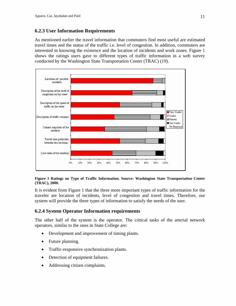
As mentioned earlier the travel information that commuters find most useful are estimated travel times and the status of the traffic i.e. level of congestion. In addition, commuters are interested in knowing the existence and the location of incidents and work zones. Figure 1 shows the ratings users gave to different types of traffic information in a web survey conducted by the Washington State Transportation Center (TRAC) (19).

Figure 1 Ratings on Type of Traffic Information. Source: Washington State Transportation Center (TRAC), 2000.

It is evident from Figure 1 that the three more important types of traffic information for the traveler are location of incidents, level of congestion and travel times. Therefore, our system will provide the three types of information to satisfy the needs of the user.

6.2.4 System Operator Information requirements

The other half of the system is the operator. The critical tasks of the arterial network operators, similar to the ones in State College are:

• Development and improvement of timing plants.

• Future planning.

• Traffic-responsive synchronization plants.

• Detection of equipment failures.

• Addressing citizen complaints.


Most of these tasks can be improved with reliable on-line information on volumes, occupancy, speeds and incidents. In addition operators also consider it important to determine the signal control performances in real time. This information is very useful for timing and synchronization plants. With these system attributes, it is possible to provide volume, occupancy, speed and incident data to the system.

6.3 Utilization of the Available Data

The next task is to develop the methodology for interpreting the available traffic data from various detectors and cameras. This is a simple task if the output is a video image. The camera images may be used to determine the existing traffic conditions.

However the task becomes complicated when it comes to the utilization of detector data. Detector data are primarily used for traffic monitoring. Information from the detector data may be used to build models that can predict travel times, predict onset of congestion and to monitor flow patterns. Analyzing detector data is far more complicated because there are no standardized procedures.

For this project, it is required to know travel time along arterials in State College as it is one of the performance measures. An appropriate model needs to be used to predict travel time. There are several mathematical models available in the literature, and it is essential to determine the suitability of these models to the specific route and choose the most appropriate one.

A brief description of the available models in the literature is given. H. M. Zhang (20) developed a model to find the journey speed along an arterial. He defined the journey speed as the average speed for the entire arterial, and the inverse of journey speed as the average travel time. If the ideal travel time is known, it can be compared with the travel time from the model. The difference between the two variables is known, and it represents the delay.

The model is given by:

/ /(1 )c v c q cU U Uγ γ= + −

Where:γ is a weighted factor which is between 0 and 1. V/C- volume to capacity ratio, q-flow rate , Uf - free flow speed

/ exp{ }v c fVU UC

α β= −

/ 0.379 iq c

i

qU

o= ∑

∑

io is the occupancy measurement from the detector α and β are parameters and need to be defined for each specific case


Another way to determine the travel time is to know the sum of the delay and the ideal travel time: It is already know that the difference between the ideal travel time and the actual travel time is delay. Ideal travel time is easy to get if the free flow speed and the link length between intersections are known. The problem is to find a way to measure delay.

An available model to measure the actual travel time is the “Illinois Model”, which can be represented by the following equation:

The link travel time is given by

T UNDT DELAY= +

UNDT is calculated as

f

LUNDTV

=

Where L is the link length, fV is the free flow speed

The delay is given by

0 1 2 3DELAY deloc o grnratβ β β β= + + +

Where: deloc = ratio of detector setback to link length o = detector occupancy grnrat = green ratio (green time over cycle length)

0β 1β 2β 3β = regression parameters

Besides the models to predict travel time in the link, one could also build models to predict travel time in intersections. The following was the travel time model developed by Thakuriah et al (21) for signalized intersections. It determines the travel time as a function of the relative entry time. It shows the time that the vehicle enters relative to the downstream signal.

Where: v- traffic volume c- time required to clear the queue FFTT- free flow travel time R,G- red and green time respectively.

It is important to calibrate the model. The following steps list the calibration procedure. One half of the data is used to determine the parameters of the model and the second half is


used to test the model. The error term is defined as the difference between the travel time from mathematical model and the actual travel time. The parameters are changed and the best combination of parameters for which the error term is minimal is selected as the parameter set for the mathematical model. Similarly the best parameter set for all the mathematical models considered are determined. The mathematical model with the least value for the error term is chosen for predicting the travel time for the segment.

A mathematical model developed to predict travel time is site specific. That is it cannot be transferred to other segments even if they are similar. Hence it is critical that detector data be used to build a model that captures the characteristics of the segment which may be utilized for further analysis, including travel time prediction.

The second task is to construct the flow-density maps to be displayed on the internet. They are useful in representing the degree of congestion in the link. There are different methods for constructing the color code for the flow density maps. The most common are the ones based either on occupancy or the current travel time. If the flow density maps are constructed based on the occupancy (22) the following is the color code.

Occupancy Traffic State Color

<14% free flow Green

15%-33% Moderate Yellow

33%-50% Heavy Orange

>50% Stop and go Red

Table 3 Color code for the flow density map according to occupancy values

However occupancy, on its own, might not be a good indicator of the current traffic state, since there are two possible values of speed for every occupancy value. Hence a better representation of the traffic state is based on the current travel time. The term degree of congestion (r) is defined as the ratio of the current travel time to the free flow travel time.

Degree of congestion r = Current travel time Free flow travel time

Degree of congestion Traffic State Color

1-1.25 Free flow Green

1.26-2 Moderate Yellow

2.01-3 Heavy Orange

>3 Stop and go Red

Table 4 Color code for the flow density map according to degree of congestion


6.4 Determine Best Information Delivery Mechanism

The fourth task is to determine Information delivery mechanism. Commuters require information on accidents, congestion, roadwork and other events that impact their driving. The ideal delivery mechanism should relay in real-time, provide current and accurate traffic conditions that enables to achieve the dynamic route guidance functionality. Drivers would prefer to take the least time consuming route. Events or conditions that impact driving time or reduce safety can be detected and reported from traffic-flow data and travel-time data. There are several ways to this traffic information to the consumer (23).Some of them include radio communication, Internet, VMS signs, television and cable, smart cell phone, In-vehicle unit, pager, Palm PC/High Performance Computing (HPC) etc. Few of them like VMS signs and in-vehicle units are more expensive. The best method would be to deliver information over the radio. Another method for disseminating information would be via the internet. State College, being a college community, has a large proportion of people utilizing the Internet. Internet also provides video stream that has been proved to be one of the favorites with travelers because the users can easily identify the intersection and the traffic conditions. In addition, one of the most useful performance measures for the travelers is the location of incidents in which cameras play a central role. The traveler can see the incident by stream video on the internet but also the operator can post a warning in web map/web page.

The screen snap of the webpage is shown in Figure 2. It shows the traffic conditions of the study area at a particular day and time. The commuters can see congestion zones, incidents, and working spots online. Traffic conditions such as stop and go, heavy, moderate, and wide open can be displayed. Also color codes are adopted to display different levels of congestion. The web page will be updated every 5 minutes.

In addition, most of the people carry cell phones. Consequently, it would be a good idea to start a unique phone number, which will convey the current traffic information of the local area. Moreover, to the dissemination means mentioned above, television may be used to broadcast real time traffic information. Local channels can be used to disseminate the present traffic condition. A good instance would be when a major incident takes place that has a potential to disrupt traffic for a long time period, the local channels may be useful in passing on this information to the commuters which may include flashing news about nature of incident, the time duration of the incident effects. In conclusion, it is suggested that the information will be disseminated initially with the help of radio, Internet and/or television. As per the necessity in future consideration may be given for the use of smart cell phones.

GolfCours

es

BJC

HUB

CURTIN

EPA

RK

UNIVERSITY

E COLLEGE

S PUGH

EFOSTER

E POLLOCK

E BEAVER

LOCUST

N ALLEN

MCKEE

S ALLEN

S GARNER

HASTINGS

EIR

VIN

EPRO

SPEC

T

SHORTLIDGE

WPARK

HETZEL

BIGLER

EHAM

ILTO

N

RIDGE

ELM

ADAMS

PORTER

EFA

IRM

OUNT

HOLMES

HIGH

CLAY

WARIN

G

BIGLER ROAD

MCKEAN

EM

ITCHELL

ENTRANCE

S FRASER

MIFFLIN

ENIT

TANY

HIGHLAND

FRASER

BCRAILROAD

LINDEN

UN

NA

MED

STR

EET

KELLER

E CALDER

RAMP

OAK

Traffic Conditions as of: April 27, 2004 4:47 PM ET

00 0.10.1 0.20.2 0.30.30.050.05MilesMiles

Legend

Video Camera

congestion

Stop and Go

Heavy

Moderate

Wide Open

No Data

Incidents

Working Zone

Go To the Main Menu

Go to the Travel Time Calculator

Click on the camera symbols orHERE to see the video snapshots

Go to the stream video

Go to the detail incident report

FIgure 2. Example of Traffic Conditions Map for State College

Querying Tools

Zooming Tools


6.5 Install, Test, and Operate the Infrastructure

The final step is the installation and calibration of the video cameras. After installation it is imperative that the sensor be calibrated. The accuracy of sensor evaluations should be made for the operational conditions for which they are designed. Some sensors may be designed for low-volume goods. Therefore, testing those sensors under high volume traffic conditions will produce unacceptable accuracy results.

7. Conclusion

A summary of the state-of-the-art in traffic performance monitoring, including performance measures, data collection and dissemination methods were included in the report. The steps involved in the developing of a traffic monitoring set up plan were explained in detail. A realistic traffic data collection, processing, analysis and dissemination plan was discussed for the Penn State campus area. The plan included the proposed data collection plan, the exact locations and the type of equipment to be used for data collection and dissemination.


8. References

1. Dailey, D. J. (1997). Travel time estimates using a series of single loop volume and occupancy.

2. Bremmer, D., Cotton, K., Cotey, D., Prestrud, C., and Westby, G. Measuring Congestion: Learning From Operational Data. Presented at the 2004 Transportation Research Board Meeting, Washington D.C. 2004.

3. Oh, C., Ritchie, S. G., Jeng, S. Vehicle Reidentification using Heterogeneous Detection Systems. Presented at the 2004 Transportation Research Board Meeting, Washington D.C. 2004.

4. Tawfik, A., Abdulhai, B., Peng, A., Tabib,, S., Improving the accuracy of vehicle Signature Reidentification Using Decision Trees. Presented at the 2004 Transportation Research Board Meeting, Washington D.C. 2004.

5. V. Anantharam, Estimation of Travel Time Distribution and Detection of Incidents based on Automatic Vehicle Classification. California PATH Working Paper UCB-ITS-PWP-98-12, June 1998.

6. Kikuchi, S., Chakroborty, P., Estimating Travel Times on Urban Corridors using Bus Travel Time Data. Presented at the 2004 Transportation Research Board Meeting, Washington D.C. 2004.

7. Hoogendoorn, S. P., Van Zuylen, H. J., Schreuder, M., Gorte, B., Vosselman, G., Microscopic Traffic Data Collection by Remote Sensing.

8. Deriving Traffic Performance Measures and Levels of Service from Second-Order Statistical Features of Spatiotemporal Traffic Contour Maps Paper submitted for presentation at the Transportation Research Board 82nd Annual Meeting Washington, D.C. 2003 and for publication in the Transportation Research Record journal.

9. May, A. D., Traffic Flow Fundamentals, Prentice Hall, New Jersey, 1990

10. Transportation Research Board, Highway Capacity Manual, National Research Council, Washington D.C., 2000.

11. Coifman, B. 2003. Identifying the onset of congestion rapidly with existing traffic detectors. Transportation Research Part A 37(March):277-291.

12. Daganzo.R Using the input-output diagram to determine the spatial and temporal extents of a queue upstream of a bottleneck Trans. Res. Rec. 1572, pp. 140-147 (1997).


13. Zhang, Y., Hu, R. Q., Bruce, L. M., Balraj, N., Arora, S. Devepment of real-time Automated Accident Detection System at Intersection. Presented at the 2004 Transportation Research Board Meeting, Washington D.C. 2004.

14. Best ITS Management Practices and Technologies for Ohio, KHA of Ohio, Inc, prepared for Ohio DOT, July 2001.

15. Coifman, B., Yang, Y., Estimating Spatial Measures of Roadway Network Usage from Remotely Sensed Data, Presented at the 2004 Transportation Research Board Meeting, Washington D.C. 2004.

16. Advances in Transportation Data Collection and Management White Paper, Texas Transportation Institute, December 2002.

17. The Integrated Transportation Management System, Delaware DOT information brochures.

18. Henry X. Liu, Rachel He, Yang Tao, Bin Ran, A Literature and Best Practices Scan: ITS Data Management and Archiving, University of Wisconsin at Madison, submitted to the Wisconsin DOT, May 2002.

19. Nee, J., Hallenbek, M. E., Surveillance Options for Monitoring Arterial Traffic Conditions, Washington Transportation Center (TRAC), 2001.

20. Zhang, H.M. Link-Journey-Speed Model for Arterial Traffic, Transportation Research Record 1676, 1999, pp 109-115.

21. Todd L. Graves, Alan F. Karr, and Piyushimita Thakuriah Variability of Travel Times on Arterial Links: Effects of Signals and Volume, Technical Report Number 86 August, 1998.

22. Wisconsin Department of Transportation webpage, http://www.dot.wisconsin.gov/, May 2004.

23. Park, D., Rilett, L., Forecasting Multiple-Period Freeway Link Travel Times Using Modular Neural Networks, presentation, 77th Annual Meeting of the Transportation Research Board, Washington, D.C., January 1998.

Assessment on Traffic Operations Performance Measures and Data Collection/Dissemination Plan for...

Documents

Transcript of Assessment on Traffic Operations Performance Measures and Data Collection/Dissemination Plan for...