Assessment of the importance of mixing in the Yucca ...

Svensk Kärnbränslehantering ABSwedish Nuclear Fueland Waste Management Co

Box 250, SE-101 24 Stockholm Phone +46 8 459 84 00

Technical Report

TR-11-02

Assessment of the importance of mixing in the Yucca Mountain hydrogeological system

Javier B. Gómez, Luis F. Auqué, María Gimeno, Patricia Acero

Geochemical Modelling Group, Department of Earth Sciences University of Zaragoza

Zell Peterman, Thomas A. Oliver U.S. Geological Survey

Mel Gascoyne, Gascoyne Geoprojects Inc

Marcus Laaksoharju, Geopoint AB

February 2011

TR-11-02

Assessm

ent of the importance of m

ixing in the Yucca Mountain hydrogeological system

CM

Gru

ppen

AB

, Bro

mm

a, 2

011

Tänd ett lager:

P, R eller TR.

Assessment of the importance of mixing in the Yucca Mountain hydrogeological system

Javier B. Gómez, Luis F. Auqué, María Gimeno, Patricia Acero

Geochemical Modelling Group, Department of Earth Sciences University of Zaragoza

Zell Peterman, Thomas A. Oliver U.S. Geological Survey

Mel Gascoyne, Gascoyne Geoprojects Inc

Marcus Laaksoharju, Geopoint AB

February 2011

ISSN 1404-0344

SKB TR-11-02

This report concerns a study which was conducted for SKB. The conclusions and viewpoints presented in the report are those of the authors. SKB may draw modified conclusions, based on additional literature sources and/or expert opinions.

A pdf version of this document can be downloaded from www.skb.se.

TR-09-12 3

Foreword

The M3 code (Multivariate Mixing and Massbalance calculations) is a statistical and mathematical groundwater modelling tool developed by SKB which models the obtained groundwater chemistry in terms of sources and sinks in relation to an ideal mixing model. The complexity of the measured groundwater data determines the configuration of the ideal mixing model. Deviations from the ideal mixing model are interpreted as being due to reactions or other processes such as evaporation.

M3 is used as one of the major groundwater modelling tool within the SKB site investigation pro-gramme. The code has previously been applied on groundwater data from Sweden, Finland, Canada, Japan, Jordan and Gabon. There is an increasing interest to use the code for various groundwater modelling tasks in shallow and deep groundwater environments in different countries. The purpose of this report is to test the code in a challenging groundwater environment such as the Yucca Mountain. The results are used as an important validation and verification exercise of the M3 code.

TR-09-12 5

Summary

The Yucca Mountain area is the focus of a potential repository for high-level radioactive waste. The planned repository is located in the unsaturated zone at approximately 500 m below the eastern crest of Yucca Mountain. In the event of a confinement failure in the repository, contaminated waters will first percolate down to the underlying tuffaceous aquifer and then south and south-east to the Central Amargosa Valley. Here, a complex aquifer system will receive the plume and consequently it is of utmost importance to assess the degree of connection between the three main aquifers in the area: the Tertiary Tuffs Aquifer (directly connected to Yucca Mountain), the Quaternary Basin-fill Aquifer, and the regional (and deep) Palaeozoic Carbonate Aquifer. An upward leakage from the Palaeozoic Carbonate Aquifer would dilute the contaminant plume, while the reverse, downward leakage from the Tertiary Tuffs Aquifer or the Quaternary Basin-fill Aquifer into the Palaeozoic Carbonate Aquifer would contaminate a major aquifer system. The main objective of this study is to propose a mixing hypothesis for the Yucca Mountain groundwaters and to assess the degree of mixing between the different aquifers.

For this purpose, a large set of samples taken in deep and shallow boreholes, wells and springs are analysed from a hydro-geochemical point of view. These samples cover an area of ~280 km2 (40 km in the east-west direction and 90 km in the north-south direction) with the northern boundary just north of the Yucca Mountain crests and the southern boundary near the locality of Death Valley Junction, CA. There is a general northeast-southwest topographic gradient, with maximum altitudes of 2,000 m above sea level in the Eleana Range and minimum altitudes of –80 m above sea level in Death Valley, which in a general way controls the regional flow of groundwaters in the area. For local groundwater flow, the maximum relief is of the order of 1,000 m, as occurs between the top of Yucca Mountain (1,507 m above sea level) and the bottom of the Amargosa River at Ash Meadows (around 650 m above sea level).

Hydrogeologically, the movement of groundwaters can be discussed in terms of local, intermediate, and regional flow systems. The first two are relatively shallow and water flow is restricted to indi-vidual basins. whereas regional flow is deeper and water flows from one basin to another. Regional groundwater flow is mainly through faults and fractures in the thick Palaeozoic carbonate rocks, whereas intermediate and local flow is in the Cainozoic volcanics and Quaternary basin-fill deposits. These three aquifer systems have a complex geometry and are separated by aquitards with sometimes lesser known confinement characteristics.

Five different water types contributing to the chemistry of any water parcel in the Yucca Mountain area have been identified: precipitation, surface waters, perched waters, unsaturated-zone pore waters, and saturated-zone groundwaters. In addition, the saturated-zone groundwaters have been grouped into 10 hydrofacies based on chemical, geographical and hydrogeological criteria. These 10 hydro-facies are (from north to south and west to east): Western Yucca Mountain, Eastern Yucca Mountain, Bare Mountains, South East Crater Flat, Jackass Flat, Western Rock Valley, Fortymile Wash, Amargosa River, Eastern Amargosa and Ash Meadows.

The initial dataset consists of 397 water samples, of which 39 are precipitation samples, 17 surface water samples, 6 perched water samples, 81 pore water samples and 254 are groundwater samples.

The analysis of the sample dataset has been carried out in two steps: a preliminary exploratory analysis where the processes affecting the chemistry of each sample are identified, followed by a multivariate statistical analysis for the assessment of mixing. The preliminary exploratory analysis is performed on the complete dataset (raw dataset, 397 samples). It serves to identify trends and outliers and, together with PHREEQC simulations, to eliminate from the raw dataset all the samples affected by non-mixing processes (water-rock interaction, evaporation, cation exchange, etc).

6 TR-09-12

After the exploratory analysis, which was carried out in two phases, i.e. total system and by hydro-facies, a total of 157 samples were screened out. The distribution of eliminated samples is as follows:

(i) 38 precipitation samples (i.e. only one representative precipitation water, sample #6221, was retained),

(ii) 16 surface water samples because they were affected by strong water-rock interaction and evaporation (sample #275 was retained as a representative of the less evolved surface waters),

(iii) one perched water sample with a very anomalous chemistry (sample #336),

(iv) all 81 pore water samples, as the exploratory analysis showed that their chemistry was, in general, unrelated to the chemistry of the groundwaters and, in addition, cation exchange between pore waters and secondary minerals in the Tertiary tuffs was very apparent, and

(v) 18 groundwater samples (8 from the Ash Meadows hydrofacies, 4 each from the Fortymile Wash and Bare Mountains hydrofacies, and one each from the Eastern Amargosa and Western Rock Valley hydrofacies).

The main processes identified in the screened-out groundwater samples are evaporation (Ash Meadows hydrofacies), anthropic contamination (Fortymile Wash hydrofacies), calcite subsaturation in a carbonate aquifer (Bare Mountains hydrofacies), high chloride concentrations in an otherwise very diluted hydrofacies (Eastern Amargosa), and high bicarbonate, 400 mg/L, in a hydrofacies with a constant bicarbonate content of 160 mg/L (Western Rock Valley).

The final dataset (240 samples) is used as input to the multivariate geochemical code M3 in order to identify potential end-member waters and, most importantly, to bracket the number of end-members that can best explain the chemistry of the samples of the final dataset.

M3 (Multivariate Mixing and Mass balance) is a Principal Component Analysis code that approaches the modelling of mixing and mass balance from a purely geometrical perspective (Laaksoharju et al. 1999, 2009, Gómez et al. 2006, 2009). As opposed to standard geochemical codes, M3 tries first to explain the chemical composition of a parcel of water by pure mixing, and only then are deviations from the pure mixing model interpreted as chemical reactions. The M3 computer program is a stand-alone program developed by SKB in the MATLAB 7.1 computational environment. M3 has been recently subjected to a verification and validation procedure (Gómez et al. 2009).

The main outcome of the M3 analysis is the identification of mixing models that are able to explain the overall chemistry of a large dataset in terms of mixing. Given a set of potential end-member waters, M3 explores all possible combinations of end-members and ranks these mixing models in terms of the number of samples inside the mixing polyhedron (coverage). Samples inside the mixing poly hedron are those whose chemistry can be explained by a mixture of the end-member waters that define the particular mixing model. The more samples in a mixing model inside the mixing polyhedron, the better the model is at explaining the chemistry of the complete dataset.

All the best mixing models identified by M3 (14 mixing models with coverage > 75%) are composed of three end-members (5 models) or four end-members (9 models). No five-end-member mixing model can compete with the three- and four-end-member mixing models in terms of coverage. Under closer inspection, the three-end-member mixing models are clearly inferior to the four-end-member ones as they exclude important subsets of samples from the mixing polyhedron. It is thus concluded that the Yucca Mountain hydro-system is best explained as a mixture of four end-member waters.

Another important result arising from the M3 analysis is that the samples defining the end-members in the good mixing models are only a small subset of the initial set of potential end-members. In other words, only a small number of samples can act as end-member waters so that, when they mix, they can reproduce the chemistry of the Yucca Mountain hydro-system. For obvious reasons, these end-member waters have been termed the Tertiary Tuffs Aquifer (TTA) end-member, the Regional Palaeozoic Carbonate Aquifer (RCA) end-member, the Quaternary Basin-fill Aquifer (QBfA) end-member, and the Altered Meteoric Water (AMW) end-member. The first three end-members are representative of each of the major aquifer systems in the area, while the fourth is representative of the meteoric waters (a precipitation sample, a surface water sample or a perched water sample). The TTA end-member is systematically defined by sample #211 (Eastern Yucca Mountain hydrofacies); the RCA end member is defined either by sample #264 (Bare Mountains hydrofacies) or by sample #40

TR-09-12 7

(Ash Meadows hydrofacies); the QBfA end-member is defined either by sample #143 (Amargosa River hydrofacies) or by sample #291 (Jackass Flat hydrofacies); and the AMW end-member is defined either by precipitation sample #6221 or by perched water sample #345.

Six mixing models were finally selected from the initial 14 identified by M3. To rank the mixing models, two parameters have been considered: (i) coverage and (ii) a good match between the chloride contents of the actual samples and that of the reconstructed chemistry based on the computed mixing proportions. Once arranged in order, the best model has been taken as the reference mixing model. The mixing proportions computed with the reference model are the best approximation to the mixing processes that the waters at Yucca Mountain have undergone. The picture that emerges from this mixing model is the following:

1. The reference mixing model has sample #211 as the TTA end-member, sample #264 as the RCA end-member, sample #143 as the QBfA end-member, and sample #345 as the AMW end-member. The coverage is 81.4%, i.e. 195 samples out of 240 are inside the mixing polyhedron. Overall, the highest contribution to the chemistry of the samples in the final dataset comes from the AMW (49%), followed by the TTA (19%), the RCA (17%), and the QBfA (15%). Also, the AMW contribution is the most evenly spread among the samples.

2. The Eastern and Western Yucca Mountain hydrofacies samples are almost a binary mixture of the TTA and AMW end-members. The presence of an AMW component in these waters is somewhat surprising, and points to the rather widespread presence of an “old” meteoric water in many shallow sections of the local aquifers around Yucca Mountain.

3. Most Ash Meadows samples are almost a binary mixture of the RCA and AMW end-members (with a small contribution, ~8%, of the QBfA end-member). This concurs with a discharge of the regional Palaeozoic carbonate aquifer along the Gravity fault, followed by a mixture of the carbonate waters with (old) meteoric waters during ascent.

4. The samples from the Central Amargosa Valley (Amargosa River, Eastern Amargosa, Fortymile Wash, and Western Rock Valley hydrofacies) are particularly interesting because they occupy the area located down-gradient of Yucca Mountain. From the point of view of mixing, these waters are dominated by the QBfA and AMW end-members, although they always have contributions from at least one other end-member water. Based on hydrofacies, Amargosa River samples have the highest contribution of the QBfA end-member (between 75% and 100%), followed by the Eastern Amargosa samples (around 40%), and the Fortymile Wash samples (less than 20%). The Western Rock Valley samples have a varied contribution of the QBfA, between 0 and 50%. The “extra” con-tribution could be the TTA (as in one subset of the Western Rock Valley samples), the RCA (as in the Eastern Amargosa samples), or both (as in the Fortymile Wash samples). The high contribution of the RCA end-member in most samples of the Eastern Amargosa hydrofacies is compatible with their position intersecting the Gravity fault.

In summary, the ternary mixing that characterises most samples in the Central Amargosa Valley is a clear indication that the aquifers in the area are not completely sealed. On the contrary, it seems that mixing between chemically contrasting waters is widespread down-gradient of Yucca Mountain.

The study performed in this context was funded by the USGS and, apart from its intrinsic interest for the dynamics of the groundwater system at Yucca Mountain, it is highly recommended for application by any potential M3 users who may want to understand and apply the complete methodology to a different hydrogeological system. In this respect, the Yucca Mountain hydro-system has proved to be rather difficult, and the stringent methodological procedure devised to model the system could serve as a template for further studies.

TR-09-12 9

Objectives

The main objective of this work is to assess the importance of mixing on the hydrochemistry of waters in and around Yucca Mountain, most importantly in those waters south of Yucca Mountain. Due to the general north-south gradient of groundwater flow in the Yucca Mountain area, leakage from the proposed high-level radioactive waste repository would have the greatest consequences in the saturated zone waters south of Yucca Mountain. In this area (Amargosa River, Amargosa Flat and Ash Meadows), three main aquifers interact: the Regional Palaeozoic Carbonate Aquifer (RCA), the Tertiary Tuffs Aquifer (TTA) and the Quaternary Basin-fill Aquifer (QBfA). One consequence of upward leakage from the Palaeozoic Carbonate Aquifer would be to dilute the contaminant plume should one develop from the radioactive waste repository at Yucca Mountain. The reverse, down-ward leakage from the Tertiary Tuffs Aquifer or the Quaternary Basin-fill Aquifer into the Palaeozoic Carbonate Aquifer would contaminate a major aquifer system. It is clearly of the utmost importance to explore the links between theses aquifer systems and to assess the degree of mixing between the groundwaters.

To attain this general objective, the following specific objectives have been either defined in advance or decided as being important during the development of the project:

1. Compile a dataset of water samples from the Yucca Mountain area. This dataset should contain samples from all the potential water types that contribute to the chemistry of the groundwaters in the aquifer systems in the area.

2. Perform a careful total-system exploratory analysis on the initial (raw) dataset in order to identify trends and outliers.

3. Perform a detailed exploratory analysis of each individual hydrofacies with the aim of identifying and eliminating from the raw dataset all the samples heavily affected by processes other than mixing (e.g. water-rock interaction, evaporation, cation exchange). PHREEQC simulations were performed in order to conduct such screening.

4. Analyse the final dataset with the multivariate geochemical code M3 in order to identify the end-member waters needed to explain the chemistry of the groundwaters in the Yucca Mountain area.

5. Define the best mixing model and compute the mixing proportions in terms of the selected end-member waters. Particularly important are the mixing proportions of the waters down-gradient of Yucca Mountain, in the Central Amargosa River area.

TR-09-12 11

Contents

1 Introduction 131.1 Geography 131.2 Geology and hydrogeology 14

2 Analysis of hydrogeochemical data 192.1 Methodology 192.2 Hydrofacies, water types and water categories 192.3 Water types 502.4 Exploratory analysis 50

2.4.1 Total-system exploratory analysis 512.4.2 Hydrofacies exploratory analysis 622.4.3 Conclusions of the exploratory analysis 87

3 M3 analysis: selection of end-member waters and calculation of mixing proportions 89

3.1 Selection of end-member waters 893.2 Test of mixing models 943.3 Mixing proportions 99

3.3.1 Mixing model MM3 (reference mixing model) 1023.3.2 Mixing model MM5 1073.3.3 Mixing models MM1 and MM2 1083.3.4 Mixing models MM4 and MM6 1093.3.5 Comparison of mixing proportions: a final assessment 111

4 Conclusions 115

5 References 117

TR-09-12 13

1 Introduction

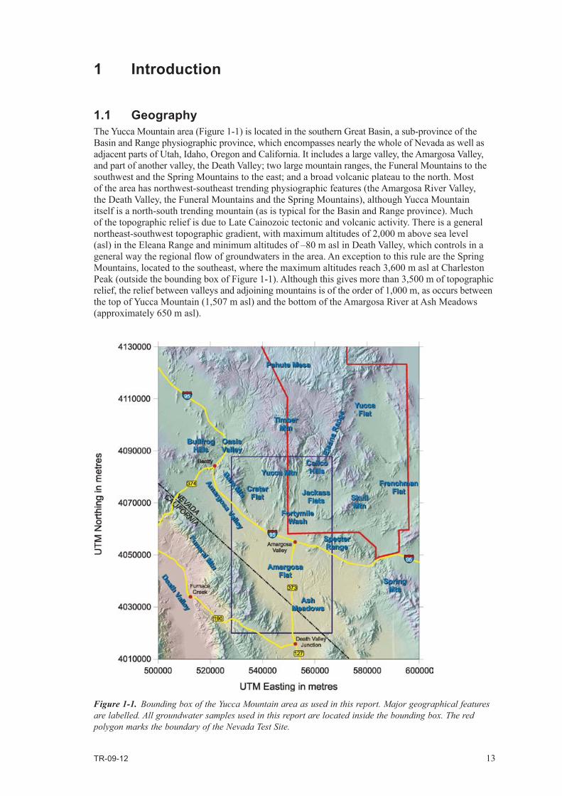
1.1 GeographyThe Yucca Mountain area (Figure 1-1) is located in the southern Great Basin, a sub-province of the Basin and Range physiographic province, which encompasses nearly the whole of Nevada as well as adjacent parts of Utah, Idaho, Oregon and California. It includes a large valley, the Amargosa Valley, and part of another valley, the Death Valley; two large mountain ranges, the Funeral Mountains to the southwest and the Spring Mountains to the east; and a broad volcanic plateau to the north. Most of the area has northwest-southeast trending physiographic features (the Amargosa River Valley, the Death Valley, the Funeral Mountains and the Spring Mountains), although Yucca Mountain itself is a north-south trending mountain (as is typical for the Basin and Range province). Much of the topographic relief is due to Late Cainozoic tectonic and volcanic activity. There is a general northeast-southwest topographic gradient, with maximum altitudes of 2,000 m above sea level (asl) in the Eleana Range and minimum altitudes of –80 m asl in Death Valley, which controls in a general way the regional flow of groundwaters in the area. An exception to this rule are the Spring Mountains, located to the southeast, where the maximum altitudes reach 3,600 m asl at Charleston Peak (outside the bounding box of Figure 1-1). Although this gives more than 3,500 m of topographic relief, the relief between valleys and adjoining mountains is of the order of 1,000 m, as occurs between the top of Yucca Mountain (1,507 m asl) and the bottom of the Amargosa River at Ash Meadows (approximately 650 m asl).

Figure 1-1. Bounding box of the Yucca Mountain area as used in this report. Major geographical features are labelled. All groundwater samples used in this report are located inside the bounding box. The red polygon marks the boundary of the Nevada Test Site.

14 TR-09-12

Mountain ranges are separated by broad intermontane basins. The basins are filled with sediment and certain interbedded volcanic deposits that gently slope from the valley floors to the bordering mountain ranges (Peterson 1981). The valley floors are local depositional centres which usually contain playas that act as catchments for surface-water runoff (Grose and Smith 1989). Most of the basins seldom contain perennial surface water and many playas contain saline deposits that indicate the evaporation of surface water and/or shallow ground water from the playa surface. Playas affected by quaternary faulting contain springs in which ground water is forced to the surface by juxtaposed lacustrine and basin-fill deposits (Bedinger et al. 1989). The Amargosa Desert contains several spring pools (e.g. Ash Meadows) and human-engineered reservoirs that are supported by regional ground-water discharge.

From a climatic point of view, most of the Yucca Mountain Area forms part of the Mojave Desert, characterised by hot, dry summers and warm, dry winters. The northern sector, however, belongs to what has been called the Transition Desert, and here the climate is a mixture of the Mojave Desert climate and the Great Basin Desert climate, the latter being characterised by warm, dry summers and cold, dry winters.

Precipitation in the region is influenced by two distinct storm patterns, one occurring in the winter and the other in the summer. Winter precipitation (dominantly snow in the mountains and rain in the valleys) tends to be of low intensity and long duration, and covers great areas. In contrast, most summer rains (resulting from local convective thunderstorms), are of high intensity and short dura-tion (Hales 1972, 1974).

The soils and vegetation are controlled to a substantial degree by climatic, geomorphic, and hydro-logic factors, and are highly variable and complex. Soils in the Yucca Mountain area typically include soils weathered from bedrock on the mountains, medium- to coarse-textured soils on alluvial fans and terraces, and fine-grained, alluvial soils on the valley floors. In general, the soils of the mountains and hills are thin and coarse textured, with little moisture-holding capacity. The soils of the alluvial fans on the upper bajadas also are coarse textured but are thicker, so that infiltration rates are relatively high. Infiltration rates of the alluvial basin soils are low because the downward movement of water is frequently impeded by calcium carbonate-cemented layers (pedogenic carbonate), fine-grained playa deposits and, less commonly, silicified hardpans that form within the soils over time (Beatley 1976).

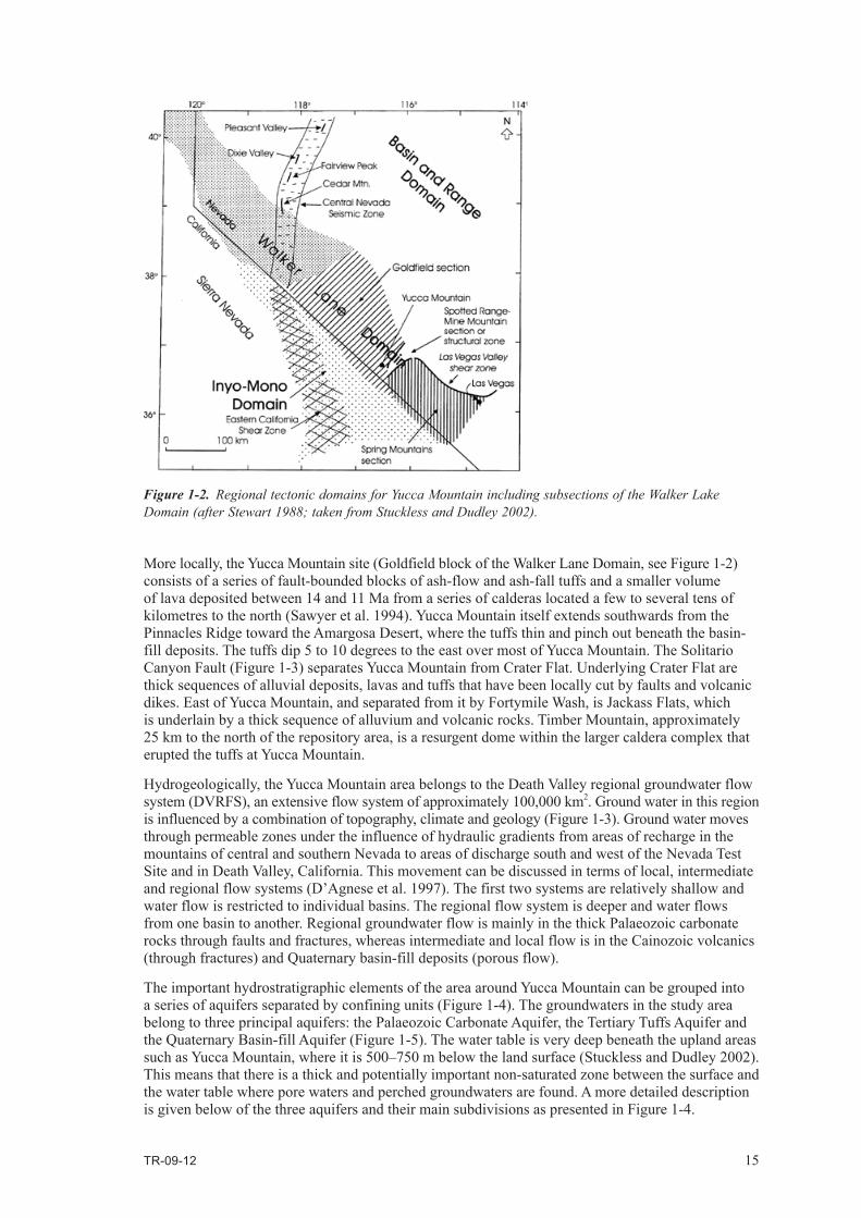
1.2 Geology and hydrogeologyThe current tectonic setting of Yucca Mountain is a result of extensional tectonism and magmatism active during the middle and late Cainozoic Era. Three regional tectonic domains characterise the tectonic setting within 100 km of Yucca Mountain (Stuckless and Dudley 2002, Sweetkind et al. 2004) (Figure 1-2): the Walker Lane Domain, which includes the site; the Basin and Range Domain to the northeast and the Inyo-Mono Domain to the southwest. These domains represent structurally bounded blocks of crust, each characterised by a deformation history that differs substantially from adjacent domains. Most of the area shown in Figure 1-1 belongs to the Walker Lane Domain.

The northwest-trending Walker Lane Domain (Stewart 1988, Stewart and Crowell 1992) is a complex structural zone that is dominated by large right-lateral faults with northwest orientations, such as the Pahrump-Stewart Valley fault zone and the Las Vegas Valley shear zone. It has been subdivided into three structural blocks according to their style of deformation (Stewart 1988, Stewart and Crowell 1992): (i) the Goldfield block occupying the north-western part and notable for its lack of full-penetration strike-slip faults and relative lack of normal faults; (ii) the Spotted Range-Mine Mountain block characterised by east-northeast-trending, left-lateral strike-slip faults, such as the Rock Valley fault zone and the Cane Spring and Mine Mountain faults; (iii) the Spring Mountains block, which is a relatively intact block that is bounded by the Pahrump-Stewart Valley fault zone and the Las Vegas Valley shear zone.

Most of the deformation in the Walker Lane belt may have occurred during Middle Miocene time (Hardyman and Oldow 1991, Dilles and Gans 1995), although deformation in the vicinity of Death Valley continued into Late Miocene time (Wright et al. 1999, Snow and Wernicke 2000). Some structures in the belt, such as the Rock Valley fault zone, continue to be active (Rogers et al. 1987, von Seggern and Brune 2000).

TR-09-12 15

More locally, the Yucca Mountain site (Goldfield block of the Walker Lane Domain, see Figure 1-2) consists of a series of fault-bounded blocks of ash-flow and ash-fall tuffs and a smaller volume of lava deposited between 14 and 11 Ma from a series of calderas located a few to several tens of kilometres to the north (Sawyer et al. 1994). Yucca Mountain itself extends southwards from the Pinnacles Ridge toward the Amargosa Desert, where the tuffs thin and pinch out beneath the basin-fill deposits. The tuffs dip 5 to 10 degrees to the east over most of Yucca Mountain. The Solitario Canyon Fault (Figure 1-3) separates Yucca Mountain from Crater Flat. Underlying Crater Flat are thick sequences of alluvial deposits, lavas and tuffs that have been locally cut by faults and volcanic dikes. East of Yucca Mountain, and separated from it by Fortymile Wash, is Jackass Flats, which is underlain by a thick sequence of alluvium and volcanic rocks. Timber Mountain, approximately 25 km to the north of the repository area, is a resurgent dome within the larger caldera complex that erupted the tuffs at Yucca Mountain.

Hydrogeologically, the Yucca Mountain area belongs to the Death Valley regional groundwater flow system (DVRFS), an extensive flow system of approximately 100,000 km2. Ground water in this region is influenced by a combination of topography, climate and geology (Figure 1-3). Ground water moves through permeable zones under the influence of hydraulic gradients from areas of recharge in the mountains of central and southern Nevada to areas of discharge south and west of the Nevada Test Site and in Death Valley, California. This movement can be discussed in terms of local, intermediate and regional flow systems (D’Agnese et al. 1997). The first two systems are relatively shallow and water flow is restricted to individual basins. The regional flow system is deeper and water flows from one basin to another. Regional groundwater flow is mainly in the thick Palaeozoic carbonate rocks through faults and fractures, whereas intermediate and local flow is in the Cainozoic volcanics (through fractures) and Quaternary basin-fill deposits (porous flow).

The important hydrostratigraphic elements of the area around Yucca Mountain can be grouped into a series of aquifers separated by confining units (Figure 1-4). The groundwaters in the study area belong to three principal aquifers: the Palaeozoic Carbonate Aquifer, the Tertiary Tuffs Aquifer and the Quaternary Basin-fill Aquifer (Figure 1-5). The water table is very deep beneath the upland areas such as Yucca Mountain, where it is 500–750 m below the land surface (Stuckless and Dudley 2002). This means that there is a thick and potentially important non-saturated zone between the surface and the water table where pore waters and perched groundwaters are found. A more detailed description is given below of the three aquifers and their main subdivisions as presented in Figure 1-4.

Figure 1-2. Regional tectonic domains for Yucca Mountain including subsections of the Walker Lake Domain (after Stewart 1988; taken from Stuckless and Dudley 2002).

16 TR-09-12

Figure 1-3. Major faults, potentiometric surface and inferred flow directions in the Yucca Mountain area. The red lines are selected faults and the blue crosses indicate the location of hydraulic head measurements. The potentiometric surface is in black (with head in metres asl) and inferred flow directions are indicated with blue arrows. The outline (purple) of the proposed repository is included (from CRWMS M&O 2007).

The oldest rocks that have some bearing on the saturated-zone groundwater flow belong to the Proterozoic confining unit, and are mainly Precambrian metasedimentary assemblages which grade upsection into Cambrian siliciclastic strata.

Resting on this confining unit is the Lower Carbonate Aquifer, the deepest and regionally most important aquifer. It has a thickness of several kilometres and is composed principally of Cambrian to Devonian dolomites and limestones, extending from central Utah to eastern California. The carbonate aquifer has negligible matrix permeability and derives its transmissivity from fractures. Just east of Yucca Mountain the aquifer was intersected by borehole UE-25 p#l at a depth of 1,244 m. At this location, the carbonate aquifer is hydrologically isolated from the overlying Tertiary units as indicated by an increase in hydraulic head of approximately 20 m at the contact (Stuckless and Dudley 2002).

Regionally, rocks from the Mississippian are fine clastic in origin, mainly argillites and shales (Eleana Formation) and behave as a confining unit (Upper Clastic Confining Unit). The regional extent of this unit is smaller than previous Palaeozoic units and it has not been intersected by bore-holes near the Yucca Mountain site. However, it extends into the Nevada Test Site. In certain places, this confining unit is overlain by another Palaeozoic carbonate aquifer, the Upper Carbonate Aquifer, which is of much less importance for the regional groundwater flow than the Lower Carbonate Aquifer.

Mesozoic rocks do not play an important role in the hydrogeology of the Yucca Mountain area, and are absent from the bounding box in Figure 1-1. The nearest outcrops are at the Spring Mountains near Las Vegas (Belcher et al. 2002). When present, they can act as an aquifer or as a confining unit, depending on their fracture density.

The Cainozoic (Miocene) saturated volcanic units at and around Yucca Mountain have been grouped into two confining layers and two aquifers depending on the welded/non-welded character of the tuffs (Figure 1-4). In the Yucca Mountain region, north- to northeast-striking faults are more likely

TR-09-12 17

Figure 1-4. Major saturated zone hydrogeologic and geologic units (Eddebbarh et al. 2003).

Figure 1-5. Simplified 3D view of the main aquifers south of Yucca Mountain (courtesy of Drew Coleman and Zell Peterman).

18 TR-09-12

than those of other orientations to be permeable because they are approximately perpendicular to the least principal stress. These faults are favourably oriented for the transport of water from the high-lands in the north (Timber Mountain, Pahute Mesa) to areas of discharge in the lower basins in the south (Amargosa Desert) and southwest (Death Valley), where it is consumed by evapotranspiration (Figure 1-6). Mineralogical alteration of the volcanic rocks (zeolitization) is more intense at depth, where it greatly diminishes rock permeability. Therefore, the deeper volcanic rocks generally impede groundwater flow and confine the underlying Palaeozoic carbonate aquifer where the Upper Clastic Confining Unit is not present (Stuckless and Dudley 2002).

As described by (Luckey et al. 1996), the Tertiary volcanic section at Yucca Mountain consists of a series of ash flow and bedded ash fall tuffs that contain minor amounts of lava and flow breccia. Ash flow tuffs range from non-welded to densely welded, and the degree of welding varies both horizon-tally and vertically in a single flow unit. Non-welded ash flow tuffs, when unaltered, have moderate to low matrix permeability but high porosity. Permeability is decreased by secondary alteration, and fractures are infrequent and often closed in the low-strength non-welded tuffs. Consequently, these rocks generally constitute laterally extensive confining units in the Yucca Mountain area. This is so in the case of the Calico Hills Formation, which constitutes the Upper Volcanic Confining Unit, and also of parts of the Lower Volcanic Confining Unit, a heterogeneous unit consisting of older tuffs, lavas and breccias.

The densely welded tuffs generally have minimal primary porosity and water-storage capacity, but they can be highly fractured. Where interconnected, fractures can easily transmit water, and highly fractured units function as aquifers, as is the case with the Topopah Spring Tuff (Upper Volcanic Aquifer) and the tuffs that form the Crater Flat Group (Lower Volcanic Aquifer). Together, the upper and lower volcanic aquifers form the Tertiary Tuffs Aquifer as used in this report.

Consolidated Cainozoic basin-fill units in the region range from late Eocene to Pliocene in age. They consist of a broad range of both volcanic and sedimentary rocks including lavas, welded and non-welded tuffs, and alluvial, fluvial, colluvial, aeolian, paludal, and lacustrine sediments. Together with the unconsolidated Cainozoic (mainly Pliocene to Holocene) basin-fill sediments (coarse-grained alluvial and colluvial deposits, fine-grained basin axis deposits, and local lacustrine limestones and spring discharge deposits), which constitute a regional unconfined aquifer, referred to in this report as the Quaternary Basin-fill Aquifer (although not all of its units are Quaternary).

Figure 1-6. Conceptual hydrogeologic cross-section through Yucca Mountain in a northwest to southeast direction showing the principal hydrostratigraphic units and the main boreholes (Stuckless and Dudley 2002).

TR-09-12 19

2 Analysis of hydrogeochemical data

2.1 MethodologyAs the main objective of this work is assessing the importance of mixing in the chemistry of the groundwaters south of Yucca Mountain, the methodology has been tailored to this end. The procedure can be summarised as follows:

1. Start with the whole dataset (which will be referred to as the “raw dataset”).2. Perform a system-wide explorative analysis with the raw dataset in order to discriminate between

conservative and non-conservative behaviour for specific elements.3. Identify outliers in the raw dataset by means of ion-ion plots and Principal Component Analysis.

These outliers are removed from the raw dataset (the focus of the work is on the general behaviour and trends in the chemistry of the different water types, and not on the peculiarities of specific samples).

4. Analyse the excluded samples one by one with PHREEQC (Parkhurst and Appelo 1999) to evaluate why they are special (i.e. which processes, natural or otherwise, have contributed to their “outlierness”).

5. Perform an explorative analysis hydrofacies by hydrofacies (ion-ion plots and PCA) to locate samples where mixing is clearly not the principal process controlling their chemistry. These samples, affected by evaporation, water-rock interaction, or cation exchange (PHREEQC simulations are used to corroborate this) are also excluded from the raw dataset.

6. Identify end-member waters in the hydrofacies-by-hydrofacies exploratory analysis.7. The above screening procedure results in a dataset in which all samples that may be suspected

of having been affected drastically by non-mixing modifications of their chemistry have been excluded. This dataset is referred to as the “final dataset”.

8. Use the end-member waters selected in (6) to calculate mixing proportions and deviations from the ideal (mixing-only) chemical composition. This step is carried out with the multivariate mixing and mass balance code M3 (Laaksoharju et al. 1999, Gómez et al. 2006, 2009).

The calculated mixing proportions for each sample are used to delineate the plausible mixing events and paths between the three main aquifer systems south of Yucca Mountain.

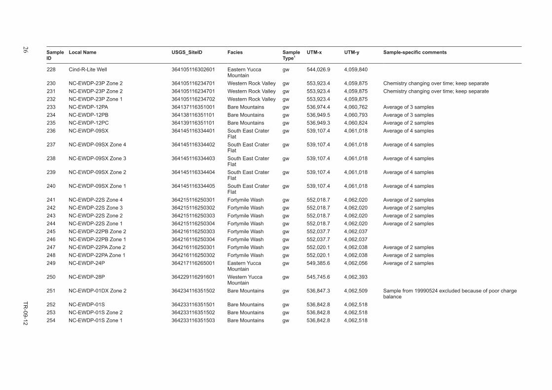
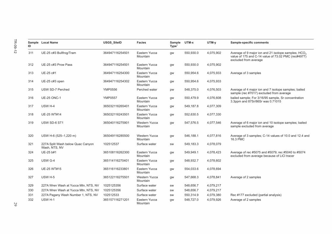
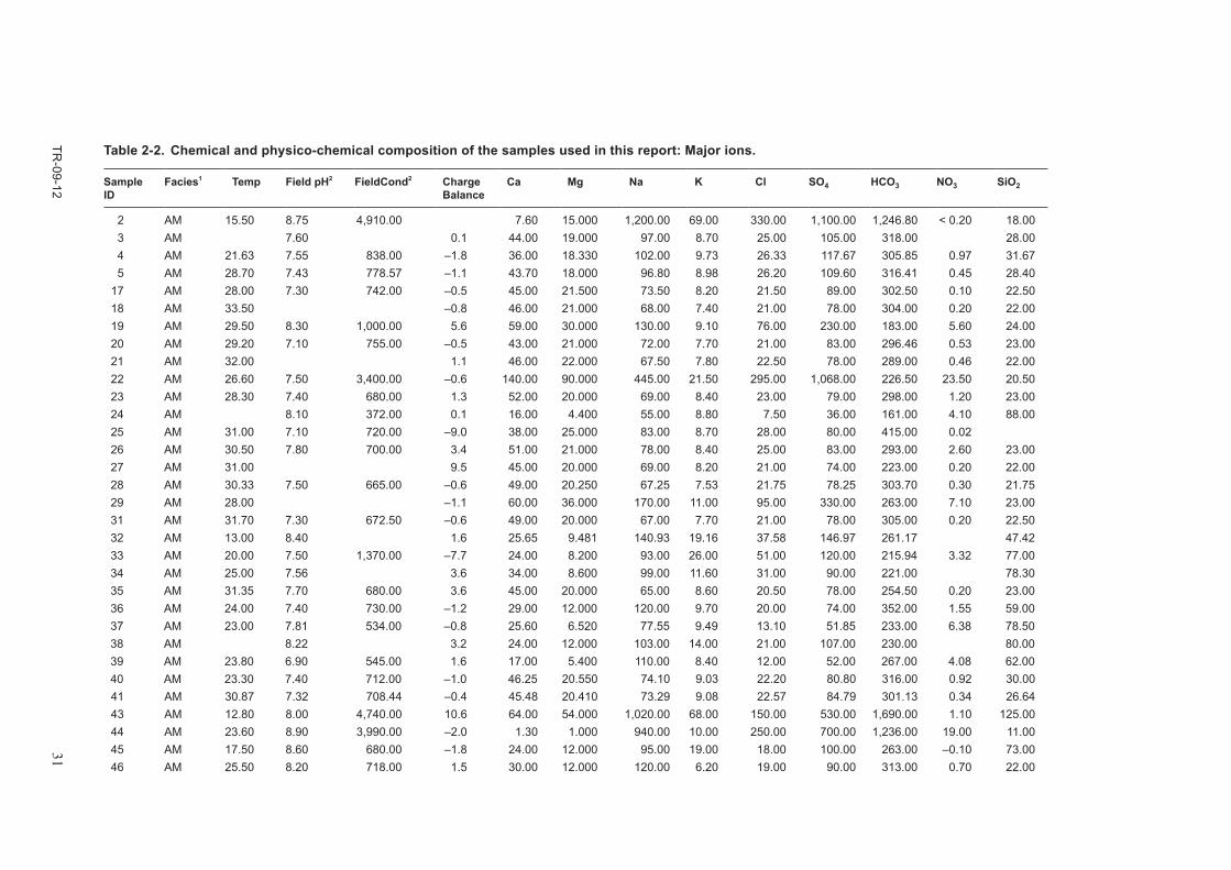
2.2 Hydrofacies, water types and water categoriesThe raw dataset consists of 397 water samples, of which 254 are groundwater samples, 6 are perched water samples, 81 are pore water samples, 17 are surface water samples, and 39 are precipitation sam-ples. The data are summarised here for each sample location of the raw dataset in Tables 2-1 (location), 2-2 (major ions) and 2-3 (isotopes, minor ions and trace elements). Where multiple sets of data were available for a sampling point, the values have been averaged to derive the value shown in the table. The column headed “Sample-specific comments” in Table 2-1 shows this information for all the samples affected. Because the data collected in the table come from multiple sources, organisations and methods, and were collected over a time span of more than 20 years, the analytical precision and accuracy vary for different chemical analyses. As a rough estimate of the analytical accuracy, the following values can be used for recent measurements (CRWMS M&O 2007):

• ±10%formajoranions,cationsandstrontiumconcentration,exceptforfluoride(±15%).Insomecases strontium was determined by isotopic dilution mass spectrometry, for which data eller the datafromwhicharemoreaccurate(±0.5%),

• ±3‰forδ2H,±0.2‰forδ18O,δ13C,andδ34S,and±0.1pmCfor14C, • Betterthan1%forUandfrom0.09%to4.5%(meanof0.73%)for234U/238U,• ±1·10–5 for 87Sr/86Srand±0.01‰forδ87Sr.

An additional guide to the reliability of individual water analyses is also provided by the calculated charge-balance errors listed in Table 2-2. Groundwaters from most sites used in this analysis have charge-balanceerrorsoflessthan±5%(85%ofthesamples),theremainderbeingmostlyintherange±5%to±15%.Whennochargebalanceisgivenforasample(8cases),itisbecausesomeoftheionsused to compute the charge balance (usually nitrate and/or phosphate) are below the detection limit.

20 TR

-09-12

Table 2-1. Summary of water samples.

Sample ID

Local Name USGS_SiteID Facies Sample Type1

UTM-x UTM-y Sample-specific comments

2 Grapevine Springs YMP0350 Ash Meadows sp 562,403.1 4,020,635.83 Last Chance Spring 362120116162201 Ash Meadows sp 565,249.4 4,023,430 Integrated major ion and isotope samples4 Bole Spring 362145116161301 Ash Meadows sp 565,467.9 4,024,201.9 Average of 3 samples5 Big Spring 362230116162001 Ash Meadows sp 565,158.7 4,025,555.4 Average of 10 samples

17 Jack Rabbit Spring 362405116161305 Ash Meadows sp 564,823.9 4,027,001.1 Average of 2 major ion and 2 isotope samples; Rec #3829 and rec #3823 excluded from average

18 Indian Rock Spring 362343116160802 Ash Meadows sp 565,565.0 4,027,838.619 Well #3 362358116160101 Ash Meadows gw 565,961.5 4,028,11920 East of Point of Rock Springs YMP0367 Ash Meadows gw 565,986.4 4,028,119.221 King Pool 362407116162401 Ash Meadows sp 565,362.5 4,028,268.5 Average of 2 samples22 Well #2 362409116155601 Ash Meadows gw 565,636.5 4,028,270.6 Average of 2 samples23 18S/51E–7cbc YMP0369 Ash Meadows sp 564,938.8 4,028,296.124 18S/51E–07dac YMP0370 Ash Meadows sp 565,635.8 4,028,36325 WELL 18S/51E–07db Ash Meadows YMP0371 Ash Meadows gw 565,560.3 4,028,454.926 Well #4 362358116163301 Ash Meadows gw 565,012.1 4,028,481.627 Many Springs YMP0372 Ash Meadows sp 565,335.7 4,028,514.828 Point of Rocks (King) 362410116161002 Ash Meadows sp 565,410.4 4,028,515.4 Average of 4 samples; C-14 values were 1.7 and 11.1 PMC29 Well #1 362410116160901 Ash Meadows gw 565,958.4 4,028,519.531 Point of Rocks (Small) 362410116161001 Ash Meadows sp 565,508.9 4,028,670.2 Average of 2 samples32 18S/50E–7aa YMP0374 Ash Meadows gw 556,040.0 4,029,15833 GMC (King) Spring YMP0375 Ash Meadows sp 555,840.4 4,029,219 Sr isotope data is average of 2 samples34 18S/49E–11bbb YMP0377 Ash Meadows gw 551,306.8 4,029,28335 Well #5 362432116165701 Ash Meadows gw 564,333.1 4,029,339.3 Average of 2 samples36 Tenneco Well #3 362451116254100 Ash Meadows gw 551,278.6 4,029,83837 Mom’s Place 362444116251001 Ash Meadows gw 552,050.5 4,029,873 Average of 2 samples38 18S/50E–6dac YMP0380 Ash Meadows gw 556,034.8 4,029,95939 Tenneco Well #2 362459116251000 Ash Meadows gw 552,049.2 4,030,08940 Ash Meadows Ranger Station YMP0942 Ash Meadows gw 559,643.3 4,030,38441 Crystal Pool 362502116192301 Ash Meadows sp 560,588.3 4,030,575.6 Average of 8 major ion and 9 isotope samples43 Franklin Well YMP0386 Ash Meadows gw 548,234.0 4,030,92944 Tennaco YMP0388 Ash Meadows gw 553,164.0 4,031,051

TR-09-12

21

Sample ID



45 Spring (18S/49E–1aba) YMP0387 Ash Meadows sp 554,035.5 4,031,05646 230 S17 E51 31DDD 1

Unknown362529116155801 Ash Meadows gw 565,789.3 4,031,106.6

47 Guerdon Industries Well #10 362529116171100 Ash Meadows gw 563,871.6 4,031,123 Average of 2 samples48 Devil’s Hole 362532116172700 Ash Meadows sp 563,572.4 4,031,182.4 Average of 13 major ion and 4 isotope samples49 Ash Tree Spring 362535116244200 Ash Meadows gw 552,739.7 4,031,202 Average of 3 samples51 Garners Well 362555116205301 Ash Meadows gw 558,437.9 4,031,855 Rec #3963 excluded; high TDS possibly contaminated52 Scruggs Spring 362601116182800 Ash Meadows sp 561,997.6 4,032,003 Integrated major ion and isotope samples; C-14 values

were 1.1 and 2.6 and 14.7 PMC56 Well 10 362627116213501 Ash Meadows gw 557,631.5 4,033,29858 IMV#1 YMP0402 Amargosa River gw 547,348.8 4,033,42059 IMV#2 362648116274601 Amargosa River gw 548,145.4 4,033,425 Average of 3 samples63 230 027N004E27D01S 362715116322301 Amargosa River gw 541,245.7 4,034,22181 230 S17 E50 23B 1 Five Springs Area 362723116184101 Ash Meadows sp 561,052.2 4,035,416.5 Average of 2 major ion and 2 isotope samples82 Five Springs Well 362755116190401 Ash Meadows gw 561,125.8 4,035,571.1 Average of 7 major ion and 2 isotope samples84 17S/50E–19aab 362505116223001 Ash Meadows gw 555,773.3 4,035,75185 Longstreet Spring 362751116192701 Ash Meadows sp 560,427.1 4,035,812.7 Average of 2 samples and integrated major ion and isotope

samples; C-14 values were 2.7 and 8.0 PMC86 Purgatory Spring Well 362822116193801 Ash Meadows gw 561,344.5 4,036,312.288 Gilgans South Well 362835116264101 Eastern Amargosa gw 549,744.6 4,036,731 Average of 5 samples

89 230 S17 E49 15BBD 1 Unknown

362839116263700 Eastern Amargosa gw 549,843.4 4,036,854

90 17S/50-15aca 362840116193701 Ash Meadows gw 560,568.5 4,036,953.892 Rogers Spring 362835116192101 Ash Meadows sp 560,417.9 4,037,137.6 Integrated major ion and isotope samples; C-14 values

were 1.5 and 12.1 PMC93 Soda Ash Spring 362848116195901 Ash Meadows sp 559,745.6 4,037,194.694 Well 8 362858116195301 Ash Meadows gw 559,968.0 4,037,411.895 230 S17 E49 08DDB 1

Unknown362904116280800 Fortymile Wash gw 547,574.7 4,037,612

96 Crane Domestic YMP0424 Amargosa River gw 543,591.8 4,037,93097 Lyle Records Well #2 362920116311000 Amargosa River gw 543,043.6 4,038,08199 Fairbanks Spring 362924116203001 Ash Meadows sp 559,015.9 4,038,361 Average of 13 samples; Rec #4079 (partial analysis)

excluded101 Mecca Club 362936116251500 Eastern Amargosa gw 551,873.4 4,038,623 Average of 2 samples

22 TR

-09-12

Sample ID



102 Lyle Records Well 362938116300100 Fortymile Wash gw 544,757.5 4,038,645103 AF Playa 362936116153001 Ash Meadows gw 566,428.0 4,038,722.5104 Bill Copeland Well 362940116265800 Eastern Amargosa gw 549,310.1 4,038,731105 Ponderosa Dairy #1 YMP0429 Eastern Amargosa gw 549,384.7 4,038,731106 Ponderosa Dairy #1 YMP0429 Eastern Amargosa gw 549,384.7 4,038,731107 Amargosa Motel (B) YMP0432 Eastern Amargosa gw 551,722.1 4,038,961116 230 S17 E48 01AB 2

Unknown363028116302500 Fortymile Wash gw 544,152.5 4,040,182

117 Amargosa Estates #2 YMP0448 Fortymile Wash gw 544,624.0 4,040,400120 16S/48E–36dcc 363044116303601 Amargosa River gw 543,528.2 4,040,672121 16S/48E–36dcc 363044116303601 Amargosa River gw 543,528.2 4,040,672122 Bray Domestic YMP0451 Fortymile Wash gw 546,662.2 4,040,688123 Oettinger Well YMP0455 Eastern Amargosa gw 551,685.2 4,040,963124 Good’s Well YMP0458 Eastern Amargosa gw 551,980.3 4,041,520125 16S/48E–36a YMP0459 Fortymile Wash gw 543,721.8 4,041,720126 Mill’s Well YMP0460 Eastern Amargosa gw 553,222.0 4,041,836127 Payton Domestic YMP0463 Eastern Amargosa gw 553,121.5 4,041,989128 Betty Smith Well 363128116302400 Fortymile Wash gw 544,167.9 4,042,031129 Bradshaw’s Well 363109116253101 Eastern Amargosa gw 551,454.7 4,042,071 16S/49-35ba in Buqo130 Mathew’s Well 363132116240000 Eastern Amargosa gw 553,717.1 4,042,208 Integrated major ion and isotope samples; major ion data

from rec 4155 excluded (inconsistent K value)131 Funeral Mountain Ranch Irrigation YMP0486 Fortymile Wash gw 541,376.3 4,043,311133 Anvil Ranch Irrigation 363205116271801 Fortymile Wash gw 548,785.1 4,043,566136 Jacob’s #1 363219116302400 Fortymile Wash gw 544,159.9 4,043,602137 DeLee Large Irrigation 363203116295801 Fortymile Wash gw 544,806.4 4,043,606138 16S/48E–23da YMP0495 Fortymile Wash gw 542,390.7 4,044,364139 Jacob’s #2 363249116291900 Fortymile Wash gw 545,771.2 4,044,535140 Rancho Amargosa Well 363252116323000 Fortymile Wash gw 541,022.0 4,044,604141 Fox Well YMP0903 Fortymile Wash gw 542,414.0 4,044,672142 230 S16 E48 23AA 1 363244116320701 Fortymile Wash gw 541,318.9 4,044,913143 Ohataz Well YMP0497 Amargosa River gw 536,122.0 4,045,105144 T&T Ranch 363313116302500 Fortymile Wash gw 544,126.5 4,045,266145 Thiede’s Well YMP0498 Fortymile Wash gw 547,432.9 4,045,284146 Albitre Well 363320116280900 Fortymile Wash gw 547,506.3 4,045,500

TR-09-12

23

Sample ID



147 230 S16 E49 18DC 1 Unknown

363323116294400 Fortymile Wash gw 545,144.1 4,045,579

148 Ouimet’s Well YMP0500 Amargosa River gw 536,045.4 4,045,598149 Tharpe’s Well YMP0502 Amargosa River gw 534,826.7 4,045,747150 Spear’s Well 363332116323501 Fortymile Wash gw 540,519.0 4,045,834152 16S/48E–15ba YMP0506 Amargosa River gw 539,669.8 4,046,693153 230 S16 E48 17ABBB1 363342116345401 Amargosa River gw 537,035.0 4,046,712154 Schoolhouse Well YMP0505 Eastern Amargosa gw 550,407.8 4,046,718155 230 S16 E48 15AA 1 363342116325101 Fortymile Wash gw 540,787.8 4,046,821156 Selbach Domestic 363342116335701 Fortymile Wash gw 539,147.2 4,046,844157 Nichol’s Well 363405116324000 Fortymile Wash gw 540,762.8 4,046,852158 Lowe Domestic YMP0509 Eastern Amargosa gw 552,121.2 4,047,005159 Amargosa Elementary School 363410116273500 Fortymile Wash gw 548,342.9 4,047,045160 McCracken Domestic YMP0511 Amargosa River gw 537,381.5 4,047,052161 Sullivan Well YMP0512 Amargosa River gw 536,784.6 4,047,142162 K. Garey 363418116274200 Fortymile Wash gw 548,167.5 4,047,291163 Perez Well YMP0514 Eastern Amargosa gw 553,833.9 4,047,386164 230 S16 E50 07C 1 363409116233701 Eastern Amargosa gw 551,348.1 4,047,432165 Fox Well 363425116332000 Fortymile Wash gw 539,765.7 4,047,463166 Cook’s Well 363425116235000 Eastern Amargosa gw 553,932.4 4,047,540 Average of 2 samples167 Nelson Domestic 363428116240301 Eastern Amargosa gw 553,608.7 4,047,631168 Cooks East Well 363428116234701 Eastern Amargosa gw 554,006.4 4,047,633169 230 S16 E49 09CA 1 363415116275101 Fortymile Wash gw 547,941.0 4,047,782170 Henderson’s Well YMP0519 Fortymile Wash gw 546,723.1 4,047,806171 O’Neill Domestic YMP0520 Fortymile Wash gw 547,294.2 4,047,902172 Barrachman Dom/Irr YMP0523 Amargosa River gw 534,941.3 4,048,120 Average of 2 samples173 Rose Well YMP0524 Amargosa River gw 534,841.7 4,048,181174 Finley’s Well YMP0526 Amargosa River gw 534,791.2 4,048,366175 230 S16 E48 08BAAA1 363434116354001 Amargosa River gw 536,654.9 4,048,405176 K. Finicial 363456116284100 Fortymile Wash gw 546,694.7 4,048,453177 A. Sasse Well 363528116284200 Fortymile Wash gw 546,664.5 4,049,439179 230 S15 E50 25BD 1

Nye County Land Company363715116244500 Western Rock Valley gw 549,538.0 4,052,639

24 TR

-09-12

Sample ID



180 230 S15 E49 22DC 1 Unknown


181 230 S15 E50 22 7 Unknown


182 TW-5 363815116175901 Western Rock Valley gw 562,604.5 4,054,686183 230 S15 E49 22AABA1 363742116263201 Fortymile Wash gw 549,863.1 4,054,911184 Airport Well 363830116241401 Eastern Yucca

Mountaingw 552,818.2 4,054,929 Average of 4 samples

185 15S/50E–18cdc YMP0537 Western Rock Valley gw 553,934.3 4,055,151186 NDOT well 363835116234001 Western Rock Valley gw 553,685.4 4,055,242187 NDOT-2 Well 363835116234002 Western Rock Valley gw 553,685 4,055,242188 15S/50E–19b1 YMP0536 Western Rock Valley gw 553,685.4 4,055,242 Average of 2 samples189 15S/50E–18ccc YMP0540 Western Rock Valley gw 553,710.0 4,055,273 Average of 3 samples190 Desert Farms Garlic Plot (DFGP) YMP0541 Western Rock Valley gw 553,287.7 4,055,301191 NC-EWDP-04PA 363925116241501 Western Rock Valley gw 553,253.7 4,056,780 Average of 4 samples192 NC-EWDP-04PB 363925116241401 Western Rock Valley gw 553,278.5 4,056,780 Chemistry changing over time; keep separate193 NC-EWDP-04PB 363925116241401 Western Rock Valley gw 553,278.5 4,056,780 Chemistry changing over time; keep separate194 NC-EWDP-04PB 363925116241401 Western Rock Valley gw 553,278.5 4,056,780 Chemistry changing over time; keep separate195 NC-EWDP-04PB 363925116241401 Western Rock Valley gw 553,278.5 4,056,780 Chemistry changing over time; keep separate196 NC-EWDP-04PB 363925116241401 Western Rock Valley gw 553,278.5 4,056,780 Chemistry changing over time; keep separate197 NC-EWDP-02D 363939116275401 Fortymile Wash gw 547,814.1 4,057,180 bailed198 NC-EWDP-Washburn-1X 363951116252402 Fortymile Wash gw 551,544.5 4,057,569199 NC-EWDP-15P 364011116295001 Eastern Yucca


200 NC-EWDP-05SB 364011116223401 Western Rock Valley gw 555,752.0 4,058,214 Chemistry changing over time; keep separate201 NC-EWDP-05SB 364011116223401 Western Rock Valley gw 555,752.0 4,058,214 Chemistry changing over time; keep separate202 NC-EWDP-19D 364014116265301 Eastern Yucca

Mountaingw 549,322.3 4,058,267 Average of 3 samples; sample collected on 20031029

excluded from average203 NC-EWDP-19D Zones 1–4 YMP0921 Eastern Yucca


204 NC-EWDP-19D Zone 1 YMP0922 Eastern Yucca Mountain

gw 549,322.3 4,058,267


gw 549,322.3 4,058,267


gw 549,322.3 4,058,267

TR-09-12

25

Sample ID




gw 549,322.3 4,058,267 Collected at end of tracer test


gw 549,322.3 4,058,267 Average of 2 samples





211 NC-EWDP-19D Zone 5–7 YMP0926 Eastern Yucca Mountain

gw 549,322.3 4,058,267

212 NC-EWDP-19P 364015116265301 Eastern Yucca Mountain


213 NC-EWDP-19 IM-1 364015116265302 Eastern Yucca Mountain

gw 549,322.1 4,058,297

214 NC-EWDP-19IM1 Zone 5 364015116265302 Eastern Yucca Mountain



gw 549,322.1 4,058,297


gw 549,322.1 4,058,297


gw 549,322.1 4,058,297



219 NC-EWDP-19IM2 364015116265201 Eastern Yucca Mountain

gw 549,347.0 4,058,298 Average of 2 samples; sample collected on 20031028 excluded from average

220 NC-EWDP-19PB Zone 2 364014116264801 Eastern Yucca Mountain

gw 549,336.7 4,058,316

221 NC-EWDP-19PB Zone 1 364014116264802 Eastern Yucca Mountain

gw 549,336.7 4,058,316

224 NC-EWDP-03S Zone 3 364054116321302 Western Yucca Mountain

gw 541,348.3 4,059,457 Average of 3 samples; uranium concentration ranges from 4 ug/L to 18 ug/L

225 NC-EWDP-03S Zone 2 364054116321303 Western Yucca Mountain

gw 541,348.3 4,059,457 Average of 2 samples; sample colleced on 20031105 excluded from average because of contamination

226 NC-EWDP-03D 364054116321401 Western Yucca Mountain




26 TR

-09-12

Sample ID



228 Cind-R-Lite Well 364105116302601 Eastern Yucca Mountain

gw 544,026.9 4,059,840

230 NC-EWDP-23P Zone 2 364105116234701 Western Rock Valley gw 553,923.4 4,059,875 Chemistry changing over time; keep separate231 NC-EWDP-23P Zone 2 364105116234701 Western Rock Valley gw 553,923.4 4,059,875 Chemistry changing over time; keep separate232 NC-EWDP-23P Zone 1 364105116234702 Western Rock Valley gw 553,923.4 4,059,875233 NC-EWDP-12PA 364137116351001 Bare Mountains gw 536,974.4 4,060,762 Average of 3 samples234 NC-EWDP-12PB 364138116351101 Bare Mountains gw 536,949.5 4,060,793 Average of 3 samples235 NC-EWDP-12PC 364139116351101 Bare Mountains gw 536,949.3 4,060,824 Average of 2 samples236 NC-EWDP-09SX 364145116334401 South East Crater

Flatgw 539,107.4 4,061,018 Average of 4 samples

237 NC-EWDP-09SX Zone 4 364145116334402 South East Crater Flat








241 NC-EWDP-22S Zone 4 364215116250301 Fortymile Wash gw 552,018.7 4,062,020 Average of 2 samples242 NC-EWDP-22S Zone 3 364215116250302 Fortymile Wash gw 552,018.7 4,062,020 Average of 2 samples243 NC-EWDP-22S Zone 2 364215116250303 Fortymile Wash gw 552,018.7 4,062,020 Average of 2 samples244 NC-EWDP-22S Zone 1 364215116250304 Fortymile Wash gw 552,018.7 4,062,020 Average of 2 samples245 NC-EWDP-22PB Zone 2 364216116250303 Fortymile Wash gw 552,037.7 4,062,037246 NC-EWDP-22PB Zone 1 364216116250304 Fortymile Wash gw 552,037.7 4,062,037247 NC-EWDP-22PA Zone 2 364216116250301 Fortymile Wash gw 552,020.1 4,062,038 Average of 2 samples248 NC-EWDP-22PA Zone 1 364216116250302 Fortymile Wash gw 552,020.1 4,062,038 Average of 2 samples249 NC-EWDP-24P 364217116265001 Eastern Yucca


250 NC-EWDP-28P 364229116291601 Western Yucca Mountain

gw 545,745.6 4,062,393

251 NC-EWDP-01DX Zone 2 364234116351502 Bare Mountains gw 536,847.3 4,062,509 Sample from 19990524 excluded because of poor charge balance

252 NC-EWDP-01S 364233116351501 Bare Mountains gw 536,842.8 4,062,518253 NC-EWDP-01S Zone 2 364233116351502 Bare Mountains gw 536,842.8 4,062,518254 NC-EWDP-01S Zone 1 364233116351503 Bare Mountains gw 536,842.8 4,062,518

TR-09-12

27

Sample ID



255 NC-EWDP-01DX 364234116351501 Bare Mountains gw 536,842.8 4,062,518 Bailed256 NC-EWDP-01DX Zone 2 364234116351502 Bare Mountains gw 536,842.8 4,062,518 Sample from 19990524 excluded because of poor charge

balance258 NC-EWDP-16P 364329116291901 Western Yucca

Mountaingw 545,665.4 4,064,263 Sample from 20050920 excluded because of possible

contamination from construction materials259 NC-EWDP-7SC Zone 4 364332116332203 Bare Mountains gw 539,631.9 4,064,317260 NC-EWDP-7SC Zone 3 364332116332204 Bare Mountains gw 539,631.9 4,064,317 Average of 2 samples261 NC-EWDP-7SC Zone 2 364332116332205 Bare Mountains gw 539,631.9 4,064,317 Average of 2 samples262 NC-EWDP-7SC Zone 1 364332116332206 Bare Mountains gw 539,631.9 4,064,317 Average of 2 samples263 NC-EWDP-7S 364332116332201 Bare Mountains gw 539,638.1 4,064,317264 NC-EWDP-7SC 364332116332202 Bare Mountains gw 539,638.1 4,064,317265 NC-EWDP-10S Zone 2 364349116241801 Fortymile Wash gw 553,140.0 4,064,899 Average of 2 samples266 NC-EWDP-10S Zone 1 364349116241802 Fortymile Wash gw 553,140.0 4,064,899 Average of 2 samples267 NC-EWDP-10P Zone 2 364349116241701 Fortymile Wash gw 553,148.8 4,064,916 Average of 2 samples268 NC-EWDP-10P Zone 1 364349116241702 Fortymile Wash gw 553,148.8 4,064,916 Average of 2 samples269 NC-EWDP-10S YMP0941 Fortymile Wash gw 553,128.5 4,064,945270 NC-EWDP-27P 364402116294801 Western Yucca


272 NC-EWDP-13P YMP0943 South East Crater Flat

gw 543,471.2 4,066,433



274 JF-3 364528116232201 Fortymile Wash gw 554,498.3 4,067,974275 40-Mile Wash at J-12 364551116233700 Surface water sw 554,121.9 4,068,680276 Well MR3 364556116413501 Amargosa River gw 527,395.0 4,068,707 Average of 3 samples; C-14 value from 19890916

(1999 C-14 value excluded)277 NECO Well #1 364600116413001 Amargosa River gw 527,518.9 4,068,738 Average of 6 samples278 MW315 364557116411801 Amargosa River gw 527,816.4 4,068,739279 MW604 364557116411501 Amargosa River gw 527,890.8 4,068,739280 MW311 364557116411401 Amargosa River gw 527,915.6 4,068,739281 UE-25 J-12 364554116232401 Fortymile Wash gw 554,443.6 4,068,775 Average of 8 major ion and 3 isotope samples; All samples

collected before borehole deepened in 1968 excluded282 MW 314 364600116412001 Amargosa River gw 527,766.5 4,068,831283 U.S. Ecology-W001 364601116414101 Amargosa River gw 527,245.8 4,068,860284 MW 316 364603116410801 Amargosa River gw 528,063.7 4,068,924

28 TR

-09-12

Sample ID



285 Precip Gauge, Waste Burial Site South of Beatty, Nv

364606116413101 Precipitation me 527,493.2 4,069,015

286 MW 313 364615116412401 Amargosa River gw 527,665.8 4,069,293 Average of 2 samples287 MW 600 364615116412402 Amargosa River gw 527,665.8 4,069,293 Average of 2 samples288 Precip Area 25 364652116172001 Precipitation me 563,454.8 4,070,624289 UE-25 WT#12 364656116261601 Eastern Yucca

Mountaingw 550,168.1 4,070,659 Average of 7 major ion and 8 isotope samples

290 HRF Precipitation 364704116170302 Precipitation me 563,873.4 4,070,997291 UE-25 J-11 364706116170601 Jackass Flat gw 563,798.6 4,071,058 Average of 8 major ion and 4 isotope samples293 USW VH-1 364732116330701 South East Crater

Flatgw 539,975.5 4,071,714 Average of 5 major ion and 4 isotope samples

294 Busted Butte Wash 364749116235100 Surface water sw 553,751.9 4,072,314295 UE-25 WT#3 364757116245801 Eastern Yucca


296 USW VH-2 365821116343701 Bare Mountains gw 537,738.3 4,073,214 Average of 5 major ion and 3 isotope samples297 UE-25 WT #17 364822116262601 Eastern Yucca

Mountaingw 549,904.7 4,073,307 Average of 3 samples; three samples collected duiring

early pumping excluded because of possible contamination298 USW WT-10 364825116290501 Western Yucca


299 UE-25 J-13 364828116234001 Fortymile Wash gw 554,016.7 4,073,548 Average of 9 major ion and 14 isotope samples301 40-Mile Wash at Road H 364904116234700 Surface water sw 553,836.4 4,074,625302 40-Mile Wash above Drill Hole Wash 364908116234600 Surface water sw 553,860.4 4,074,749303 Drill Hole at Wash Mouth 364911116235200 Surface water sw 553,711.2 4,074,840304 Drillhole Wash CSG 10251254 Surface water sw 553,711 4,074,902305 UE-25 WT-7 364933116285701 Western Yucca

Mountaingw 546,151.2 4,075,474

306 UE-25 p#1 (0–1200 m) 364938116252100 Western Yucca Mountain

gw 551,501.2 4,075,659 Thief sample

307 UE-25 p#1 (1,300–1,800 m) 364938116252102 Eastern Yucca Mountain

gw 551,501.2 4,075,659 For 6/15/98 sample, Sr concentration 0.0225ppm and 87Sr/86Sr was 0.70961

308 USW H-3 HTH 364942116280000 Western Yucca Mountain

gw 547,561.7 4,075,759

309 UE-25 c#2 open 364947116254301 Eastern Yucca Mountain

gw 550,954.9 4,075,871 Values differ in (Claassen (1985) times may be incorrect

310 UE-25 c#2 Prow Pass 364947116254301 Eastern Yucca Mountain

gw 550,954.9 4,075,871

TR-09-12

29

Sample ID



311 UE-25 c#3 Bullfrog/Tram 364947116254501 Eastern Yucca Mountain

gw 550,930.0 4,075,902 Average of 9 major ion and 21 isotope samples; HCO3 value of 175 and C-14 value of 73.02 PMC (rec#4977) excluded from average

312 UE-25 c#3 Prow Pass 364947116254501 Eastern Yucca Mountain

gw 550,930.0 4,075,902

313 UE-25 c#1 364947116254300 Eastern Yucca Mountain


314 UE-25 c#3 open 364947116254302 Eastern Yucca Mountain

gw 550,954.6 4,075,933

315 USW SD-7 Perched YMP0556 Perched water pw 548,375.0 4,076,503 Average of 4 major ion and 7 isotope samples; bailed sample (rec #7017) excluded from average

316 UE-25 ONC-1 YMP0557 Eastern Yucca Mountain

gw 550,479.9 4,076,608 bailed sample; For 3/16/95 sample, Sr concentration 3.3ppm and 87Sr/86Sr was 0.71015

317 USW H-4 365032116265401 Eastern Yucca Mountain

gw 549,187.8 4,077,309

318 UE-25 WT#14 365032116243501 Eastern Yucca Mountain

gw 552,630.5 4,077,330

319 USW SD-6 ST1 365040116275901 Western Yucca Mountain

gw 547,576.5 4,077,546 Average of 6 major ion and 10 isotope samples; bailed sample excluded from average

320 USW H-6 (525–1,220 m) 365049116285500 Western Yucca Mountain

gw 546,188.1 4,077,816 Average of 3 samples; C-14 values of 10.0 and 12.4 and 16.3 PMC

321 227A Split Wash below Quac Canyon Wash, NTS, NV

102512537 Surface water sw 549,183.3 4,078,079

324 UE-25 b#1 365108116262300 Eastern Yucca Mountain

gw 549,949.1 4,078,423 Average of rec #5075 and #5079; rec #5040 to #5074 excluded from average because of LiCl tracer

325 USW G-4 365114116270401 Eastern Yucca Mountain

gw 548,932.7 4,078,602

326 UE-25 WT#15 365116116233801 Eastern Yucca Mountain

gw 554,033.6 4,078,694

327 USW H-5 365122116275501 Western Yucca Mountain


329 227A Wren Wash at Yucca Mtn, NTS, NV 1025125356 Surface water sw 548,656.7 4,079,217330 227A Wren Wash at Yucca Mtn, NTS, NV 1025125356 Surface water sw 548,656.7 4,079,217331 227A Pagany Wash Number 1, NTS, NV 102512533 Surface water sw 550,314.9 4,079,380 Rec #177 excluded (partial analysis)332 USW H-1 365157116271201 Eastern Yucca


30 TR

-09-12

Sample ID



333 227A Yucca Wash nr Mouth, Nevada Test Site, NV

10251252 Surface water sw 554,025.4 4,079,988


10251252 Surface water sw 554,025.4 4,079,988


10251252 Surface water sw 554,025.4 4,079,988

336 Specie Spring 365207116393201 Perched water sp 530,403.7 4,080,149 Average of 5 samples337 USW UZ-14 365208116274001 Eastern Yucca

Mountaingw 548,031.8 4,080,261 Average of 2 samples; both samples bailed

338 USW UZ-14 Perched 365208116274001 Perched water pw 548,031.8 4,080,261 Average of 2 major ion and 4 isotope samples; bailed samples and early pump samples excluded from average

340 USW WT-24 Saturated Zone 365301116271301 Eastern Yucca Mountain

gw 548,690.9 4,081,898 bailed sample

341 USW WT-24 Perched 365301116271301 Perched water pw 548,690.9 4,081,898 Average of 2 samples Bailed samples (rec #5193 to rec #5199) excluded from average

343 Overland Flow in Fortymile Canyon 365320116231501 Surface water sw 554,578.7 4,082,519344 USW G-2 365322116273501 Eastern Yucca

Mountaingw 548,142.7 4,082,542 Average of 5 major ion and 7 radioisotope samples

345 Cottonwood Spring 365353116233501 Perched water sp 554,077.1 4,083,533350 ST3 Precipitation me 565,435.804 4,085,318.96354 Topopah Spring 365620116160901 Perched water sp 565,080.8 4,088,140 Two samples from 1950s excluded (rec #7074 and 7075)355 ST2 Precipitation me 566,766.554 4,088,188.01357 Overland Flow Near Pah Canyon 365627116223701 Surface water sw 555,481.6 4,088,287359 UE-29 a #1 365629116222601 Fortymile Wash gw 555,753.3 4,088,351 Integrated 1 major ion and 3 isotope samples; rec #5314

(poor charge balance) excluded from average360 UE-29 a #2 365629116222602 Fortymile Wash gw 555,753.3 4,088,351 Average of 3 samples361 Pah Canyon Above Mouth 365634116221501 Surface water sw 556,024.4 4,088,506363 ST1 Precipitation me 565,880.739 4,088,794.35364 ST1 Precipitation me 565,880.739 4,088,794.35426 RT3 Precipitation me 563,189.256 4,109,018.47427 RT3 Precipitation me 563,189.256 4,109,018.47428 227B Stockade Wash at Airport Road,

NTS, NV102512484 Surface water sw 563,092.2 4,109,296

443 RT2 Precipitation me 569,484.623 4,112,544.89444 RT2 Precipitation me 569,484.623 4,112,544.891 gw: groundwater; me: meteoric water (precipitation); pw: pore water; sp: groundwater from spring; sw: surface water.

TR-09-12

31

Table 2-2. Chemical and physico-chemical composition of the samples used in this report: Major ions.

Sample ID

Facies1 Temp Field pH2 FieldCond2 ChargeBalance

Ca Mg Na K Cl SO4 HCO3 NO3 SiO2

2 AM 15.50 8.75 4,910.00 7.60 15.000 1,200.00 69.00 330.00 1,100.00 1,246.80 < 0.20 18.003 AM 7.60 0.1 44.00 19.000 97.00 8.70 25.00 105.00 318.00 28.004 AM 21.63 7.55 838.00 –1.8 36.00 18.330 102.00 9.73 26.33 117.67 305.85 0.97 31.675 AM 28.70 7.43 778.57 –1.1 43.70 18.000 96.80 8.98 26.20 109.60 316.41 0.45 28.40

17 AM 28.00 7.30 742.00 –0.5 45.00 21.500 73.50 8.20 21.50 89.00 302.50 0.10 22.5018 AM 33.50 –0.8 46.00 21.000 68.00 7.40 21.00 78.00 304.00 0.20 22.0019 AM 29.50 8.30 1,000.00 5.6 59.00 30.000 130.00 9.10 76.00 230.00 183.00 5.60 24.0020 AM 29.20 7.10 755.00 –0.5 43.00 21.000 72.00 7.70 21.00 83.00 296.46 0.53 23.0021 AM 32.00 1.1 46.00 22.000 67.50 7.80 22.50 78.00 289.00 0.46 22.0022 AM 26.60 7.50 3,400.00 –0.6 140.00 90.000 445.00 21.50 295.00 1,068.00 226.50 23.50 20.5023 AM 28.30 7.40 680.00 1.3 52.00 20.000 69.00 8.40 23.00 79.00 298.00 1.20 23.0024 AM 8.10 372.00 0.1 16.00 4.400 55.00 8.80 7.50 36.00 161.00 4.10 88.0025 AM 31.00 7.10 720.00 –9.0 38.00 25.000 83.00 8.70 28.00 80.00 415.00 0.0226 AM 30.50 7.80 700.00 3.4 51.00 21.000 78.00 8.40 25.00 83.00 293.00 2.60 23.0027 AM 31.00 9.5 45.00 20.000 69.00 8.20 21.00 74.00 223.00 0.20 22.0028 AM 30.33 7.50 665.00 –0.6 49.00 20.250 67.25 7.53 21.75 78.25 303.70 0.30 21.7529 AM 28.00 –1.1 60.00 36.000 170.00 11.00 95.00 330.00 263.00 7.10 23.0031 AM 31.70 7.30 672.50 –0.6 49.00 20.000 67.00 7.70 21.00 78.00 305.00 0.20 22.5032 AM 13.00 8.40 1.6 25.65 9.481 140.93 19.16 37.58 146.97 261.17 47.4233 AM 20.00 7.50 1,370.00 –7.7 24.00 8.200 93.00 26.00 51.00 120.00 215.94 3.32 77.0034 AM 25.00 7.56 3.6 34.00 8.600 99.00 11.60 31.00 90.00 221.00 78.3035 AM 31.35 7.70 680.00 3.6 45.00 20.000 65.00 8.60 20.50 78.00 254.50 0.20 23.0036 AM 24.00 7.40 730.00 –1.2 29.00 12.000 120.00 9.70 20.00 74.00 352.00 1.55 59.0037 AM 23.00 7.81 534.00 –0.8 25.60 6.520 77.55 9.49 13.10 51.85 233.00 6.38 78.5038 AM 8.22 3.2 24.00 12.000 103.00 14.00 21.00 107.00 230.00 80.0039 AM 23.80 6.90 545.00 1.6 17.00 5.400 110.00 8.40 12.00 52.00 267.00 4.08 62.0040 AM 23.30 7.40 712.00 –1.0 46.25 20.550 74.10 9.03 22.20 80.80 316.00 0.92 30.0041 AM 30.87 7.32 708.44 –0.4 45.48 20.410 73.29 9.08 22.57 84.79 301.13 0.34 26.6443 AM 12.80 8.00 4,740.00 10.6 64.00 54.000 1,020.00 68.00 150.00 530.00 1,690.00 1.10 125.0044 AM 23.60 8.90 3,990.00 –2.0 1.30 1.000 940.00 10.00 250.00 700.00 1,236.00 19.00 11.0045 AM 17.50 8.60 680.00 –1.8 24.00 12.000 95.00 19.00 18.00 100.00 263.00 –0.10 73.0046 AM 25.50 8.20 718.00 1.5 30.00 12.000 120.00 6.20 19.00 90.00 313.00 0.70 22.00

32 TR

-09-12

Sample ID



47 AM 33.40 7.90 667.00 –1.1 46.00 20.000 69.50 8.35 20.00 84.00 300.50 0.20 23.5048 AM 32.96 7.43 684.40 –0.3 49.74 21.420 67.75 7.86 22.43 80.67 306.72 0.72 22.7449 AM 21.27 7.90 372.00 –2.5 15.00 4.470 52.00 8.23 6.77 37.33 157.00 5.75 79.3351 AM 16.50 7.50 1,460.00 72.00 64.000 150.00 26.00 97.00 230.00 527.00 < 0.44 62.0052 AM 35.00 8.00 668.00 0.4 46.00 22.000 68.00 8.40 21.00 76.00 302.00 0.00 25.0056 AM 19.40 7.60 1,067.00 2.0 2.80 2.900 250.00 15.00 26.00 105.00 494.00 0.00 67.0058 AR 21.00 7.60 3.9 54.00 15.000 160.00 15.90 70.00 187.00 271.00 71.9059 AR 25.00 7.58 790.00 –0.8 45.17 10.180 102.33 11.67 28.90 92.17 299.00 10.95 70.9763 AR 22.20 7.80 943.00 1.3 58.00 19.000 134.00 19.00 32.00 107.00 438.00 0.20 72.0081 AM 34.15 7.31 600.00 0.9 46.50 20.500 70.00 7.95 20.50 81.00 289.50 0.25 22.0082 AM 33.92 7.33 695.33 –1.5 45.71 20.000 67.71 8.09 22.29 81.86 296.86 0.22 21.8684 AM 16.00 8.60 1.1 7.60 8.500 252.00 27.00 70.00 176.00 416.00 42.6185 AM 27.20 7.43 600.00 –0.3 49.50 18.000 68.50 7.85 19.50 76.50 301.00 0.35 22.0086 AM 34.50 7.30 670.00 –2.2 44.00 21.000 60.00 8.60 22.00 80.00 286.00 0.10 22.0088 EA 24.20 8.03 308.58 –0.8 19.43 1.950 40.67 7.51 9.01 29.70 125.95 7.46 77.3789 EA 22.50 8.10 321.00 –3.0 21.00 4.000 32.00 8.20 10.00 35.00 120.00 7.09 73.0090 AM 19.40 7.60 665.00 –0.4 50.00 20.000 67.00 9.20 23.00 79.00 305.00 0.90 23.0092 AM 7.60 677.00 0.2 47.00 21.000 69.00 7.80 21.00 78.00 302.00 0.00 23.0093 AM 7.70 772.00 –0.9 36.00 17.000 106.00 10.00 27.00 93.00 330.00 0.00 35.0094 AM 21.00 0.3 22.00 11.000 110.00 15.00 22.00 74.00 296.00 0.50 31.0095 FmW 24.00 8.00 299.00 1.5 21.00 2.700 36.00 7.50 6.40 27.00 123.00 6.65 81.0096 AR 26.30 7.19 1,120.00 –0.5 64.00 18.000 147.00 16.00 41.00 138.00 451.00 9.30 45.0097 AR 7.70 1,290.00 –1.5 74.00 24.000 160.00 16.00 78.00 180.00 404.00 30.57 46.0099 AM 27.72 7.33 690.00 47.13 20.100 69.31 7.97 21.40 81.45 302.33 < 0.20 22.04

101 EA 23.00 8.10 798.00 –0.6 34.50 14.000 103.50 15.00 27.00 150.00 232.50 0.37 48.00102 FmW 8.00 363.00 –0.1 24.00 1.800 48.00 7.30 9.50 31.00 153.00 7.09 80.00103 AM 16.50 8.25 –0.1 9.70 10.000 130.00 18.00 32.00 66.00 315.00 1.20 23.00104 EA 7.90 422.00 –6.0 25.00 3.600 48.00 9.70 10.00 69.00 131.00 7.09 70.00105 EA 28.30 7.98 507.00 –6.0 30.00 4.500 59.00 11.00 16.00 93.00 145.00 4.39 74.00106 EA 27.0 8.00 457.00 –0.9 24.90 4.060 57.40 10.80 21.60 70.80 129.00 9.73 87.00107 EA 24.00 7.60 852.00 –1.2 49.50 18.000 97.50 14.00 27.00 151.00 286.00 1.02 43.50116 FmW 24.40 8.00 307.00 –1.9 19.00 1.500 40.00 7.10 6.30 25.00 135.00 6.65 79.00117 FmW 24.00 8.09 296.00 1.3 20.00 2.100 38.00 6.80 6.50 22.00 134.00 7.93 79.00

TR-09-12

33

Sample ID



120 AR 7.60 670.00 5.1 40.00 8.600 98.00 11.00 29.00 43.00 278.00 7.80 74.00121 AR 26.00 7.20 830.00 –1.2 55.00 9.800 100.00 13.00 33.00 110.00 300.00 9.10 70.00122 FmW 20.90 8.05 316.00 –1.1 22.00 1.800 35.00 8.80 7.90 25.00 131.00 7.48 74.00123 EA 25.20 7.51 881.00 –2.1 50.00 16.000 103.00 15.00 29.00 157.00 291.00 1.59 39.00124 EA 7.65 3.7 44.00 16.000 120.00 16.00 29.00 148.00 267.00 36.70125 FmW 23.30 7.90 700.00 0.9 70.00 3.900 62.00 9.00 61.00 107.00 142.00 17.00 82.00126 EA 7.65 1.4 45.00 20.000 110.00 16.60 24.00 156.00 288.00 42.80127 EA 20.20 7.58 933.00 –1.4 51.00 19.000 107.00 16.00 41.00 155.00 290.00 6.15 36.00128 FmW 7.90 301.00 –3.1 17.00 2.000 40.00 6.10 6.90 25.00 133.00 7.09 79.00129 EA 24.40 7.41 796.00 0.9 53.00 18.000 113.00 13.00 31.00 170.00 278.50 0.50 37.50130 EA 7.76 3.4 52.00 22.000 120.00 17.80 27.00 168.00 309.00 37.80131 FmW 22.20 8.21 479.00 –3.1 12.00 2.400 80.00 7.00 12.00 43.00 200.00 6.59 87.00133 FmW 20.50 7.92 681.00 –1.4 47.00 5.800 68.00 13.00 40.00 120.00 138.00 20.80 71.00136 FmW 7.90 324.00 –2.3 19.00 0.800 43.00 7.30 9.30 28.00 133.00 7.53 72.00137 FmW 14.60 8.02 312.00 –0.5 23.00 1.100 37.00 8.30 6.10 25.00 135.50 7.51 76.50138 FmW 24.00 8.20 1.1 22.00 2.200 69.00 6.60 27.00 67.00 134.00139 FmW 26.40 7.90 324.00 –2.7 24.00 1.100 36.00 8.20 6.60 33.00 134.00 7.09 75.00140 FmW 8.45 367.00 2.9 18.00 1.600 54.00 6.60 15.00 40.00 122.00 68.00141 FmW 8.19 5.9 16.00 1.600 56.00 6.50 9.00 35.00 125.00 77.00142 FmW 23.90 7.30 346.00 1.0 9.40 1.000 66.00 6.80 8.80 27.00 156.00 3.10 74.00143 AR 7.69 3.2 66.00 11.000 170.00 12.00 83.00 235.00 235.00 78.00144 FmW 27.00 7.00 321.00 0.5 18.00 0.700 54.00 6.90 7.80 30.00 147.00 7.09 79.00145 FmW 7.87 0.9 30.00 2.000 40.00 4.30 8.00 51.00 130.00 77.00146 FmW 25.00 7.56 368.00 –0.3 28.00 1.800 36.00 8.30 4.70 47.00 134.20 68.00147 FmW 8.00 340.00 –2.2 20.00 2.700 42.00 8.80 7.40 28.00 150.00 6.65 59.00148 AR 7.69 2.1 53.00 8.600 150.00 10.70 63.00 187.00 232.00 77.00149 AR 7.98 1.6 55.00 11.000 150.00 11.70 61.00 190.00 267.00 79.80150 FmW 7.97 4.5 18.00 5.900 71.00 7.30 12.00 47.00 173.00 71.42152 AR 25.00 8.00 –0.2 60.00 7.800 147.00 9.80 66.00 199.00 264.00 37.00153 AR 23.90 7.40 1,074.00 0.3 60.00 7.800 157.00 12.00 69.00 179.00 302.00 1.20 75.00154 EA 23.80 7.70 650.00 –1.6 41.00 7.600 80.00 9.70 23.00 130.00 195.00 0.50 46.00155 FmW 7.70 381.00 –0.3 12.00 3.200 65.00 3.20 8.00 30.00 166.00 4.10 76.00156 FmW 23.90 7.99 631.00 –2.4 23.00 8.100 90.00 6.60 36.00 96.00 178.00 11.50 68.00

34 TR

-09-12

Sample ID



157 FmW 24.90 8.05 365.00 –2.3 9.90 3.450 59.50 5.65 5.85 32.00 161.90 6.00 65.50158 EA 18.50 7.72 855.00 –1.8 44.00 11.000 111.00 11.00 30.00 147.00 274.00 2.30 43.00159 FmW 23.30 7.60 430.00 –1.6 23.00 2.600 56.00 9.00 10.00 67.00 141.00 7.53 72.00160 AR 21.70 7.50 1,431.00 –0.7 83.00 12.000 194.00 12.00 123.00 266.00 243.00 62.00 73.00161 AR 23.30 7.60 950.00 0.3 48.00 6.800 160.00 10.00 67.00 180.00 264.00 2.90 68.00162 FmW 24.00 7.40 432.00 1.0 33.00 3.300 56.00 9.40 14.00 76.00 144.00 7.53 75.00163 EA 7.64 –7.5 46.00 17.000 120.00 4.30 24.00 160.00 284.00 20.20164 EA 7.70 821.00 0.4 51.00 18.000 103.00 13.00 30.00 143.00 288.00 0.70 31.00165 FmW 25.50 8.08 370.00 –2.5 8.85 3.400 60.50 5.60 5.90 33.00 162.30 4.50 62.50166 EA 30.70 7.46 870.00 0.4 43.50 16.500 115.00 12.50 26.50 140.00 300.00 < 0.20 25.50167 EA 29.40 7.54 897.00 –12.1 43.00 16.000 110.00 11.50 26.50 154.00 308.00 0.48 25.50168 EA 32.00 7.60 888.00 2.5 44.00 16.000 120.00 11.00 27.00 150.00 273.00 0.44 28.00169 FmW 23.90 7.20 383.00 0.9 28.00 3.400 46.00 7.60 10.00 53.00 142.00 3.30 56.00170 FmW 25.80 7.90 316.00 –1.0 23.00 2.400 37.00 6.50 6.20 29.00 138.00 6.60 58.00171 FmW 19.50 7.89 366.00 0.3 26.00 2.400 44.00 7.60 7.40 43.00 141.00 7.93 65.00172 AR 22.75 7.55 999.50 –2.5 50.20 13.300 132.00 9.51 63.15 184.00 262.00 3.69 70.00173 AR 24.20 7.70 960.00 0.0 47.00 16.000 130.00 9.20 62.00 180.00 239.00 2.50 64.00174 AR 24.70 7.40 980.00 0.0 53.00 9.400 140.00 10.00 63.00 180.00 251.00 1.90 69.00175 AR 25.00 7.90 1,160.00 1.3 59.00 6.300 180.00 13.00 80.00 203.00 296.00 38.00176 FmW 23.00 7.00 314.00 –0.2 30.00 2.600 37.00 5.60 7.70 30.00 152.00 6.65 54.00177 FmW 7.80 307.00 2.9 29.00 2.200 35.00 5.20 6.00 26.00 135.00 7.53 62.00179 WRV 44.00 7.90 343.50 –1.3 22.00 1.300 49.00 2.55 7.45 38.00 149.00 0.34 20.50180 FmW 7.80 337.00 –0.6 28.00 2.100 39.00 4.90 6.70 33.00 146.00 7.09 49.00181 FmW 6.70 325.00 –0.2 27.00 2.000 43.00 4.60 8.50 33.00 149.00 6.20 49.00182 WRV 30.00 7.80 875.00 –1.6 33.00 17.000 130.00 12.00 21.00 99.00 395.00 19.00183 FmW 27.80 8.00 336.00 –0.9 25.00 2.400 41.00 5.20 8.00 33.00 145.00 3.50 52.00184 EYM 27.55 8.69 353.00 –1.6 6.20 0.254 69.00 1.65 7.70 47.25 126.81 6.61 40.00185 WRV 25.10 8.00 492.00 –0.5 12.00 0.700 93.00 3.90 17.00 78.00 153.00 6.40 38.00186 WRV 26.31 8.00 548.09 –0.6 16.54 0.816 102.03 3.84 14.17 109.81 155.71 9.56 43.95187 WRV 27.6 8.10 569.00 –0.1 17.40 0.940 104.00 3.76 12.70 113.00 160.00 9.47 47.00188 WRV 23.90 8.05 743.00 –1.3 20.00 3.900 107.50 6.00 17.50 127.50 162.00 6.50 44.00189 WRV 8.37 487.00 –0.1 15.67 1.500 106.00 4.23 19.33 109.00 161.00 4.55 39.33190 WRV 26.20 7.78 523.00 –0.7 30.00 2.100 71.00 5.10 13.00 117.00 125.00 4.08 40.00

TR-09-12

35

Sample ID



191 WRV 23.7 7.50 334.25 –1.7 13.45 0.330 57.73 2.89 7.43 53.33 116.50 6.59 31.75192 WRV 23.5 7.90 396.00 –1.5 19.00 0.480 63.00 3.10 9.90 79.00 109.00 9.50 33.00193 WRV 23.6 9.30 359.00 –0.2 7.50 0.040 72.00 2.10 5.60 37.00 152.31 3.85 33.00194 WRV 25.9 9.20 353.00 –2.2 6.50 0.047 69.00 1.80 5.40 36.00 154.31 31.00195 WRV 23.2 9.90 316.00 –1.0 6.20 0.030 60.00 1.80 5.50 31.00 130.48 2.36 32.00196 WRV 25.4 9.30 308.00 –2.7 4.90 0.000 61.00 1.40 5.40 26.00 138.50 2.68 38.00197 FmW 7.50 301.00 –4.3 19.00 1.200 42.00 4.10 6.10 22.00 149.00 5.73 49.00198 FmW 7.70 295.00 0.1 21.00 2.700 38.00 5.60 6.90 27.00 128.00 8.29 52.00199 EYM 29.9 7.80 434.00 –1.3 10.00 2.450 81.50 3.35 8.75 44.50 188.00 4.62 49.50200 WRV 23.4 7.20 769.00 –2.6 23.00 2.800 136.00 9.30 31.00 125.00 268.00 1.23 27.00201 WRV 7.60 573.00 –0.3 14.00 1.700 107.00 6.90 32.00 61.00 211.00 0.56 21.00202 EYM 30.23 8.73 461.67 –1.2 1.73 0.056 107.50 3.60 6.22 28.00 246.85 3.41 61.00203 EYM 31.0 8.60 438.50 –3.4 2.25 0.150 96.50 3.40 6.25 22.00 238.50 3.89 57.00204 EYM 32.0 8.90 448.00 0.5 1.50 0.057 104.00 3.80 5.90 21.00 238.84 1.25 57.00205 EYM 8.40 391.50 –0.7 5.90 0.560 79.00 3.60 6.30 23.00 190.00 3.79 59.00206 EYM 28.6 8.40 384.00 3.7 7.80 0.800 76.00 4.30 6.50 21.00 175.00 58.00207 EYM 8.00 314.00 16.00 1.700 49.50 3.85 6.30 21.00 144.00 < 0.20 56.00208 EYM 28.9 8.25 327.00 0.4 10.65 0.975 60.50 3.75 6.30 21.50 153.00 5.73 60.50209 EYM 30.8 8.45 440.50 –0.4 1.30 0.050 99.00 3.20 6.30 26.00 219.00 5.14 55.00210 EYM 31.3 8.85 469.00 –1.0 0.93 0.033 107.50 3.40 5.65 18.50 256.00 2.08 60.00211 EYM 30.9 8.90 475.00 –1.0 0.57 0.027 113.00 3.51 5.50 20.30 268.74 2.24 60.40212 EYM 29.20 8.05 294.50 –2.1 16.00 1.215 47.00 3.65 7.80 22.00 141.52 4.81 54.00213 EYM 8.60 422.00 –0.7 2.88 0.219 96.00 3.30 6.30 26.20 218.61 4.43 56.70214 EYM 31.00 8.83 433.67 –1.3 0.55 0.050 101.33 3.14 5.55 17.00 244.91 2.08 58.37215 EYM 30.90 9.00 450.00 –6.3 0.57 0.030 95.90 3.24 5.50 17.30 255.77 2.03 59.10216 EYM 29.70 8.60 439.00 –3.7 1.08 0.033 98.10 3.40 6.25 25.70 235.49 4.42 56.75217 EYM 29.10 8.50 366.00 –4.4 5.62 0.464 76.90 3.30 6.10 22.00 200.52 3.84 56.20218 EYM 25.77 8.73 396.33 –1.1 2.55 0.285 93.07 3.21 5.71 19.87 223.33 2.06 54.47219 EYM 8.70 408.00 0.7 4.14 0.343 90.90 3.37 6.50 27.08 205.22 56.58220 EYM 8.20 382.00 –4.9 8.40 0.730 76.00 3.40 5.80 21.00 214.00 4.30 56.00221 EYM 8.40 328.00 –2.8 13.00 1.400 55.00 4.30 6.50 28.00 153.00 4.80 43.00224 WYM 32.60 8.87 608.67 0.81 0.097 136.67 2.93 9.53 47.33 304.06 < 0.22 48.17225 WYM 32.20 8.65 565.50 –0.6 0.78 0.090 127.50 3.30 18.00 47.50 248.30 1.57 59.00

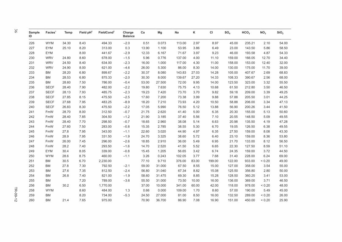
36 TR

-09-12

Sample ID



226 WYM 34.30 8.43 494.33 –2.0 0.51 0.073 113.00 2.97 8.97 45.00 235.21 2.10 54.00227 EYM 25.10 8.20 313.00 0.3 13.90 1.100 53.95 3.86 6.49 23.00 143.50 5.86 58.50228 EYM 8.00 441.67 –2.9 12.33 6.167 71.67 3.97 9.23 46.00 193.58 4.87 54.33230 WRV 24.80 8.60 678.00 –1.5 5.96 0.776 137.00 4.00 11.10 159.00 166.05 12.70 34.40231 WRV 24.50 8.40 634.00 –2.3 16.00 1.000 117.00 4.30 11.00 158.00 153.00 12.40 32.00232 WRV 24.90 8.00 621.00 –4.6 26.00 5.300 86.00 8.30 14.00 130.00 175.00 11.70 39.00233 BM 28.20 6.80 899.67 –2.2 30.37 8.080 143.83 27.03 14.28 105.00 407.67 2.69 68.83234 BM 28.53 6.80 875.33 –2.0 30.30 8.000 139.67 27.20 14.33 108.33 390.67 2.56 68.00235 BM 28.60 7.50 786.00 –0.4 53.00 27.500 72.00 9.95 14.00 123.50 323.00 3.32 55.50236 SECF 28.40 7.90 482.00 –2.2 19.80 7.630 75.75 4.13 10.68 61.50 212.80 3.50 46.50237 SECF 28.13 7.93 485.75 –2.3 19.23 7.420 73.70 3.70 9.82 59.18 209.00 3.39 49.25238 SECF 27.85 8.15 475.50 –2.5 17.60 7.200 73.38 3.99 9.88 57.88 205.50 3.01 44.25239 SECF 27.68 7.95 483.25 –8.9 18.20 7.210 73.93 4.20 10.50 58.88 206.00 3.34 47.13240 SECF 26.83 8.30 475.50 –2.2 17.05 5.990 76.50 5.12 13.88 56.90 200.26 3.44 41.50241 FmW 28.70 8.00 312.50 –0.7 21.75 2.620 41.40 5.00 6.35 20.30 155.00 5.13 50.60242 FmW 28.40 7.85 304.50 –1.2 21.90 3.185 37.40 5.56 7.10 20.55 148.50 5.09 49.55243 FmW 28.40 7.70 298.50 –0.7 18.65 2.960 38.08 5.14 6.63 20.98 135.50 4.19 47.28244 FmW 27.60 7.50 283.00 –0.8 15.35 2.785 38.55 5.30 6.70 19.05 126.50 6.38 49.55245 FmW 27.8 7.95 343.00 –1.1 22.60 3.020 44.90 4.97 6.35 27.50 159.00 8.08 43.30246 FmW 28.9 7.95 331.50 –1.9 24.70 3.325 38.60 5.72 6.40 23.10 159.00 8.36 53.80247 FmW 26.00 7.45 296.00 –2.6 18.85 2.910 36.00 5.49 6.95 21.70 133.00 8.12 56.50248 FmW 28.2 7.40 293.50 –1.6 14.70 2.520 41.50 5.52 6.65 22.30 127.50 8.59 51.10249 EYM 30.4 8.05 339.00 –0.8 15.45 1.205 56.65 3.42 6.74 24.35 159.00 3.72 44.50250 WYM 28.6 8.75 460.00 –1.1 3.26 0.243 102.05 3.77 7.68 31.40 228.00 6.24 69.00251 BM 30.5 6.70 2,230.00 77.10 9.710 376.00 83.00 199.00 122.00 933.00 < 0.20 49.00252 BM 27.8 7.30 792.50 –2.1 59.00 31.000 67.50 8.55 15.00 127.00 358.00 3.54 55.00253 BM 27.6 7.35 812.50 –2.4 56.80 31.040 67.34 8.82 15.08 125.50 356.80 2.80 50.00254 BM 26.8 7.40 821.00 –1.9 58.60 31.475 69.30 8.85 15.28 128.50 360.25 3.41 53.00255 BM 7.20 789.00 –3.6 55.50 31.000 73.50 10.00 16.00 136.00 369.00 3.71 46.50256 BM 30.2 6.50 1,770.00 37.00 10.000 341.00 60.00 42.00 118.00 978.00 < 0.20 48.00258 WYM 8.60 484.00 1.3 0.66 0.000 109.00 1.70 8.60 57.00 190.00 5.49 45.00259 BM 8.20 734.00 –5.3 24.50 27.000 81.00 8.50 16.00 132.50 289.00 < 0.20 26.00260 BM 21.4 7.65 975.00 70.90 36.700 86.90 7.08 16.90 151.00 450.00 < 0.20 25.90

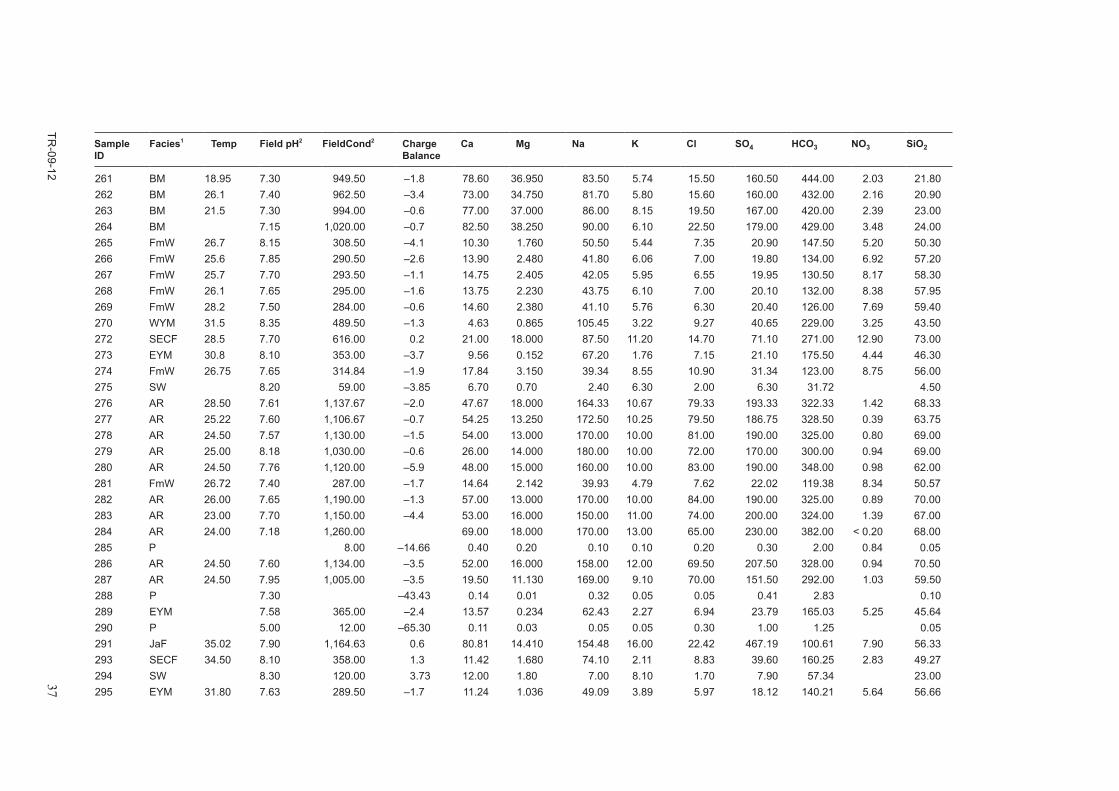
TR-09-12

37

Sample ID



261 BM 18.95 7.30 949.50 –1.8 78.60 36.950 83.50 5.74 15.50 160.50 444.00 2.03 21.80262 BM 26.1 7.40 962.50 –3.4 73.00 34.750 81.70 5.80 15.60 160.00 432.00 2.16 20.90263 BM 21.5 7.30 994.00 –0.6 77.00 37.000 86.00 8.15 19.50 167.00 420.00 2.39 23.00264 BM 7.15 1,020.00 –0.7 82.50 38.250 90.00 6.10 22.50 179.00 429.00 3.48 24.00265 FmW 26.7 8.15 308.50 –4.1 10.30 1.760 50.50 5.44 7.35 20.90 147.50 5.20 50.30266 FmW 25.6 7.85 290.50 –2.6 13.90 2.480 41.80 6.06 7.00 19.80 134.00 6.92 57.20267 FmW 25.7 7.70 293.50 –1.1 14.75 2.405 42.05 5.95 6.55 19.95 130.50 8.17 58.30268 FmW 26.1 7.65 295.00 –1.6 13.75 2.230 43.75 6.10 7.00 20.10 132.00 8.38 57.95269 FmW 28.2 7.50 284.00 –0.6 14.60 2.380 41.10 5.76 6.30 20.40 126.00 7.69 59.40270 WYM 31.5 8.35 489.50 –1.3 4.63 0.865 105.45 3.22 9.27 40.65 229.00 3.25 43.50272 SECF 28.5 7.70 616.00 0.2 21.00 18.000 87.50 11.20 14.70 71.10 271.00 12.90 73.00273 EYM 30.8 8.10 353.00 –3.7 9.56 0.152 67.20 1.76 7.15 21.10 175.50 4.44 46.30274 FmW 26.75 7.65 314.84 –1.9 17.84 3.150 39.34 8.55 10.90 31.34 123.00 8.75 56.00275 SW 8.20 59.00 –3.85 6.70 0.70 2.40 6.30 2.00 6.30 31.72 4.50276 AR 28.50 7.61 1,137.67 –2.0 47.67 18.000 164.33 10.67 79.33 193.33 322.33 1.42 68.33277 AR 25.22 7.60 1,106.67 –0.7 54.25 13.250 172.50 10.25 79.50 186.75 328.50 0.39 63.75278 AR 24.50 7.57 1,130.00 –1.5 54.00 13.000 170.00 10.00 81.00 190.00 325.00 0.80 69.00279 AR 25.00 8.18 1,030.00 –0.6 26.00 14.000 180.00 10.00 72.00 170.00 300.00 0.94 69.00280 AR 24.50 7.76 1,120.00 –5.9 48.00 15.000 160.00 10.00 83.00 190.00 348.00 0.98 62.00281 FmW 26.72 7.40 287.00 –1.7 14.64 2.142 39.93 4.79 7.62 22.02 119.38 8.34 50.57282 AR 26.00 7.65 1,190.00 –1.3 57.00 13.000 170.00 10.00 84.00 190.00 325.00 0.89 70.00283 AR 23.00 7.70 1,150.00 –4.4 53.00 16.000 150.00 11.00 74.00 200.00 324.00 1.39 67.00284 AR 24.00 7.18 1,260.00 69.00 18.000 170.00 13.00 65.00 230.00 382.00 < 0.20 68.00285 P 8.00 –14.66 0.40 0.20 0.10 0.10 0.20 0.30 2.00 0.84 0.05286 AR 24.50 7.60 1,134.00 –3.5 52.00 16.000 158.00 12.00 69.50 207.50 328.00 0.94 70.50287 AR 24.50 7.95 1,005.00 –3.5 19.50 11.130 169.00 9.10 70.00 151.50 292.00 1.03 59.50288 P 7.30 –43.43 0.14 0.01 0.32 0.05 0.05 0.41 2.83 0.10289 EYM 7.58 365.00 –2.4 13.57 0.234 62.43 2.27 6.94 23.79 165.03 5.25 45.64290 P 5.00 12.00 –65.30 0.11 0.03 0.05 0.05 0.30 1.00 1.25 0.05291 JaF 35.02 7.90 1,164.63 0.6 80.81 14.410 154.48 16.00 22.42 467.19 100.61 7.90 56.33293 SECF 34.50 8.10 358.00 1.3 11.42 1.680 74.10 2.11 8.83 39.60 160.25 2.83 49.27294 SW 8.30 120.00 3.73 12.00 1.80 7.00 8.10 1.70 7.90 57.34 23.00295 EYM 31.80 7.63 289.50 –1.7 11.24 1.036 49.09 3.89 5.97 18.12 140.21 5.64 56.66

38 TR

-09-12

Sample ID



296 BM 32.37 7.03 891.33 –1.6 78.40 30.000 70.40 8.10 15.40 141.40 397.00 1.48 26.20297 EYM 28.70 7.25 291.33 –0.2 9.66 0.666 49.63 2.45 6.39 18.16 129.73 4.69 40.10298 WYM 38.70 8.39 404.50 –0.7 2.60 0.038 96.00 0.95 7.80 33.50 195.97 4.40 46.50299 FmW 30.53 7.29 287.57 –1.2 12.89 2.010 43.95 4.96 7.24 19.29 125.93 7.72 59.73301 SW 21.30 8.00 170.00 3.25 21.00 2.90 8.20 9.10 1.40 10.00 91.50 24.00302 SW 8.40 70.00 –5.24 8.10 0.90 4.10 5.60 1.30 6.20 43.92 8.70303 SW 8.30 100.00 –1.00 9.50 1.30 8.60 7.40 2.20 12.00 51.24 20.00304 SW 8.40 125.00 0.56 11.00 1.10 8.10 6.30 2.40 4.20 53.00 6.23 22.00305 WYM 8.70 422.00 –0.4 2.40 1.900 98.50 1.95 13.00 7.20 252.00 0.02 20.00306 WYM 57.00 6.70 1,220.00 –3.0 94.00 31.000 150.00 12.00 26.00 78.00 753.00 44.00307 EYM 56.00 6.60 1,330.00 –2.3 100.00 39.000 150.00 12.00 28.00 160.00 694.00 41.00308 WYM 26.50 9.20 523.00 –11.7 0.80 0.020 120.00 1.10 9.50 31.00 334.30 0.22 46.00309 EYM 36.60 7.82 297.00 –2.5 12.00 0.350 53.50 2.05 7.05 22.00 140.00 6.31 53.50310 EYM 32.70 7.94 299.00 –2.9 6.08 0.032 60.63 1.22 5.74 16.73 150.00 4.40 42.20311 EYM 39.50 7.65 301.93 –0.1 11.54 0.304 54.53 1.95 6.49 19.66 136.71 5.15 54.52312 EYM 34.90 7.89 299.00 0.7 8.62 0.078 56.44 1.42 5.48 16.81 139.07 0.11 49.92313 EYM 41.47 7.57 303.67 –0.8 11.67 0.367 56.33 2.12 7.53 21.83 140.70 5.00 56.33314 EYM 40.80 7.70 298.00 –8.7 11.00 0.400 55.00 1.90 7.20 22.00 167.10 5.76 53.00315 PW 22.75 8.12 257.00 2.5 13.03 0.091 45.38 5.38 4.11 9.05 128.13 14.37 55.75316 EYM 8.70 302.00 2.7 13.30 1.100 50.60 3.60 7.10 23.60 132.90 1.20 26.50317 EYM 34.80 7.40 340.00 3.8 17.00 0.290 73.00 2.60 6.90 26.00 173.00 46.00318 EYM 7.30 256.00 –2.4 9.62 0.795 43.70 5.27 7.85 20.30 119.00 1.86 57.50319 WYM 35.0 8.35 391.50 –1.5 0.40 0.007 91.20 1.55 6.78 26.70 187.00 6.19 46.30320 WYM 38.87 8.05 379.00 –6.1 3.40 0.060 87.33 1.37 7.40 28.67 212.97 48.00321 SW 8.16 199.00 9.59 24.00 3.40 9.30 8.80 3.70 8.70 88.00 19.00324 EYM 36.60 7.29 295.50 –0.5 17.50 0.655 46.00 3.15 8.00 21.50 135.40 4.03 51.50325 EYM 35.60 7.70 312.00 3.7 13.00 0.200 57.00 2.10 5.90 19.00 139.00 45.00326 EYM 7.50 347.00 1.6 11.60 1.700 61.80 4.60 11.50 16.10 168.00 0.02 53.00327 WYM 35.90 7.85 276.50 1.9 1.95 0.010 60.00 2.10 6.35 16.00 126.50 48.00329 SW 8.20 258.00 8.05 28.00 3.90 16.00 11.00 5.80 16.00 109.00 21.00330 SW 5.50 8.00 184.00 11.39 22.79 3.06 9.00 8.22 4.61 13.00 72.00 15.00331 SW 3.40 8.00 250.00 1.04 27.84 3.28 17.00 6.99 5.24 29.00 108.00 20.00332 EYM 33.85 7.60 256.50 –7.9 5.35 0.050 51.00 2.00 5.75 18.50 144.55 43.50

TR-09-12

39

Sample ID



333 SW 7.00 7.60 133.00 13.43 15.00 2.30 11.00 4.10 4.40 6.00 55.00 24.00334 SW 8.10 117.00 11.63 15.00 2.10 6.00 4.10 2.00 4.00 53.00 22.00335 SW 5.70 8.00 136.00 3.79 16.33 2.71 7.00 4.15 2.40 6.00 70.00 25.00336 PW 22.50 7.10 1,100.00 –5.3 147.71 41.606 24.88 7.46 0.96 4.30 810.00 61.48337 EYM 25.70 8.38 354.50 1.0 0.34 0.027 72.04 1.93 7.19 13.80 140.70 45.54338 PW 7.87 2.5 26.0 2.15 35.00 1.75 6.50 14.55 144.50 34.50340 EYM 7.88 262.00 2.6 0.28 0.034 59.10 1.59 6.71 14.90 118.76 0.11 53.20341 PW 22.95 8.36 286.00 –2.2 20.54 1.351 37.33 2.68 8.95 15.93 134.41 0.91 41.40 343 SW 5.80 8.09 164.00 8.75 20.00 2.90 8.40 4.50 2.60 8.50 72.00 23.00344 EYM 33.75 7.53 245.13 2.7 7.91 0.475 47.20 5.62 6.44 14.42 123.53 2.73 51.13345 PW 23.00 8.73 231.00 –2.0 7.05 0.916 16.30 6.38 3.03 4.88 70.42 65.17350 P 69.51 48.4 5.88 6.09 10.20 2.60 8.20 22.70354 PW 20.70 7.70 149.00 –7.4 12.09 2.868 12.35 6.55 2.55 6.44 80.00 40.86355 P 8.54 30.8 4.7 3.92 15.60 3.20 9.20 111.00357 SW 7.75 134.00 22.26 15.00 2.80 4.90 3.70 3.40 7.80 34.00 18.00359 FmW 22.20 7.55 265.00 1.4 16.00 2.390 35.60 4.31 8.34 16.50 112.00 10.32 57.20360 FmW 23.13 7.40 248.33 –3.0 10.83 0.700 41.83 1.87 9.59 19.50 108.67 6.98 42.13361 SW 7.90 145.00 11.72 16.00 2.90 8.20 4.30 4.00 7.60 55.00 30.00363 P 12.04 4.13 0.32 0.72 0.76 0.80 1.80 9.90364 P 26.87 25.4 3.79 1.94 20.40 1.80 5.40 66.90426 P 6.36 3.45 0.36 0.60 0.64 0.70 0.80 10.90427 P 27.84 15.2 2.05 1.90 7.28 0.80 3.00 36.00428 SW 4.00 7.50 122.00 10.60 15.00 3.10 6.40 4.30 3.10 6.50 54.90 24.00443 P 15.67 1.33 0.1 0.20 0.16 0.20 0.90 2.40444 P 24.58 17.5 3.04 5.70 7.28 0.90 4.00 50.901 See Table 2-4 for hydrofacies’ abbreviations.2 Figures in italics refer to lab pH or lab conductivity (when the in situ value was not measured).

40 TR

-09-12

Table 2-3. Chemical and physicochemical composition of the samples used in this report: Minor ions and isotopes.

Sample ID

Facies1 F I Br As B Sr Li U d2H d18O d13C 14C d34S d87Sr

2 AM 3.60 1.10 8,900.00 380.00 350.00 5.873 AM 1.40 –91.30 –12.40 12.414 AM 1.13 0.16 635.00 900.00 136.67 0.20 –100.40 –14.60 13.895 AM 1.43 0.16 547.00 962.50 112.86 2.90 –101.60 –13.42 –4.60 3.08 11.08

17 AM 1.60 0.16 400.00 840.00 90.00 –107.50 –14.60 –5.50 3.70 4.6218 AM 1.50 350.00 90.0019 AM 1.70 1,500.00 120.0020 AM 1.60 360.00 940.00 93.00 4.7321 AM 1.45 80.00 80.0022 AM 1.50 4,300.00 200.0023 AM 1.20 310.00 1,100.00 100.0024 AM 2.00 < 100.00 1.6025 AM 1.30 710.00 30.0026 AM 1.70 930.00 90.0027 AM 1.50 80.0028 AM 1.63 280.00 833.33 88.33 3.10 –103.00 –13.65 –5.55 6.4029 AM 1.50 120.0031 AM 1.35 475.00 820.00 88.67 2.90 –7.40 7.2032 AM33 AM 2.90 0.13 1,600.00 660.00 91.00 4.9334 AM 2.75 486.0035 AM 1.60 910.00 80.0036 AM 3.70 590.00 130.0037 AM 2.74 0.02 0.07 20.00 366.00 326.50 91.00 1.80 –103.50 –13.25 –4.58 12.30 10.3238 AM39 AM 4.50 530.00 70.0040 AM 1.87 0.05 0.10 14.50 340.50 1,003.00 97.00 2.67 –104.25 –13.45 –4.80 8.80 15.6541 AM 1.70 0.15 368.62 942.23 88.60 3.21 –102.50 –13.73 –4.30 11.00 4.6143 AM 8.00 < 10.00 1,200.00 1,400.00 4.80 2.5544 AM 15.00 12,000.0 240.00 90.0045 AM 2.90 650.00 150.0046 AM 1.60 770.00 120.00

TR-09-12

41

Sample ID


47 AM 1.75 295.00 930.00 85.0048 AM 1.54 0.15 296.86 804.63 83.13 3.33 –13.60 –5.90 3.15 4.4649 AM 2.57 285.00 230.00 65.00 –102.00 –12.40 13.8051 AM 3.2052 AM 1.70 320.00 820.00 90.00 –6.03 6.1756 AM 3.20 1,400.00 7,700.00 140.00 4.0058 AR 2.60 750.0059 AR 2.92 0.03 0.14 13.00 426.25 446.67 123.50 3.66 –103.00 –13.48 –4.96 7.60 19.40 10.5563 AR 3.60 400.00 600.00 140.00 4.2081 AM 2.10 310.00 940.00 82.50 –102.00 –13.60 –11.00 11.4082 AM 1.66 0.15 353.00 863.33 84.00 3.05 –103.75 –14.19 4.6484 AM85 AM 1.70 355.00 875.00 92.50 3.00 –103.15 –13.80 –5.80 5.35 4.7886 AM 1.60 920.00 90.0088 EA 1.61 0.01 0.05 8.90 179.54 142.97 50.00 0.75 –99.80 –13.10 –8.30 30.45 9.40 5.1789 EA 1.40 100.00 40.0090 AM 1.20 280.00 800.00 100.0092 AM 1.50 270.00 820.00 90.00 –103.15 –13.60 –5.77 6.80 4.7793 AM 2.00 950.00 770.00 100.00 –5.00 2.9094 AM 2.10 8.20 140.0095 FmW 1.40 90.00 50.00 –102.00 –13.00 27.8096 AR 3.30 0.17 577.00 674.00 177.00 3.90 –109.00 –13.40 –4.30 7.90 12.9197 AR 6.80 670.00 160.0099 AM 1.79 364.33 825.68 89.67 2.65 –103.66 –13.88 –5.16 6.28 4.98

101 EA 2.80 500.00 760.00 140.00102 FmW 1.70 100.00 60.00 –104.00 –12.70 10.00103 AM 4.34104 EA 1.20 130.00 50.00 –105.00 –12.80 18.90105 EA 1.20 0.09 274.00 248.00 58.00 2.10 –105.50 –13.30 –7.20 14.19 16.00 4.17106 EA 1.41 0.02 0.08 10.00 211.00 328.00 73.00 1.39 –100.50 –13.20 –8.00 19.20 10.00107 EA 2.95 0.13 481.50 954.00 148.00 1.60 –109.00 –13.65 –3.00 1.94 5.58116 FmW 1.70 80.00 50.00 –104.00 –13.00 18.40

42 TR

-09-12

Sample ID


117 FmW 1.60 0.05 150.00 129.00 50.00 1.20 –104.25 –13.10 –10.60 21.60 5.16120 AR 2.80 280.00 700.00 100.00 2.90121 AR 2.80 460.00 140.00122 FmW 0.97 0.06 130.00 101.00 43.00 1.50 –103.00 –13.20 –10.00 23.50 3.43123 EA 3.30 0.14 490.00 915.00 152.00 1.40 –108.50 –13.80 –2.55 1.40 5.71124 EA 3.90 920.00125 FmW 1.40 4.70126 EA 4.00 1,100.00127 EA 3.90 0.22 481.00 1,069.00 163.00 1.00 –109.70 –13.80 –2.65 3.30 5.73128 FmW 1.60 60.00 40.00 –98.50 –12.60129 EA 4.05 420.00 1,035.00 180.00 1.60130 EA 1.80 1,080.00 –104.00 –13.70 –4.40131 FmW 2.30 0.09 227.00 114.00 60.00 1.30 –107.00 –13.70 –5.40 6.50 10.49133 FmW 1.10 0.21 279.00 319.00 53.00 2.00 –104.20 –13.10 –10.40 11.80 3.82136 FmW 1.30 80.00 50.00 –102.00 –13.00 19.30137 FmW 1.10 0.05 141.00 109.50 43.50 1.50 –104.13 –13.25 –8.43 20.50 3.51138 FmW139 FmW 1.00 60.00 40.00 –101.00 –13.10 20.80140 FmW 1.70 100.00 70.00 –99.00 –11.90 –8.40 28.42141 FmW 2.10 120.00 –99.00 –13.20 –8.40 27.40142 FmW 2.00 150.00 1,800.00 60.00 2.20143 AR 1.60 530.00144 FmW 1.50 80.00 80.00145 FmW 0.62 185.00 –97.50 –13.20 –5.20 24.80146 FmW 0.60 120.00 40.00 –97.50 –11.60 –5.20 25.81147 FmW 1.20 70.00 40.00 –102.00 –12.60 28.40148 AR 4.80 430.00 –104.00 –13.60 –5.70149 AR 1.66 520.00150 FmW 2.02 180.00152 AR153 AR 1.20 570.00 600.00 200.00 6.20154 EA 0.80 350.00 60.00 –105.00 –13.80 –3.40155 FmW 3.00 90.00 0.00

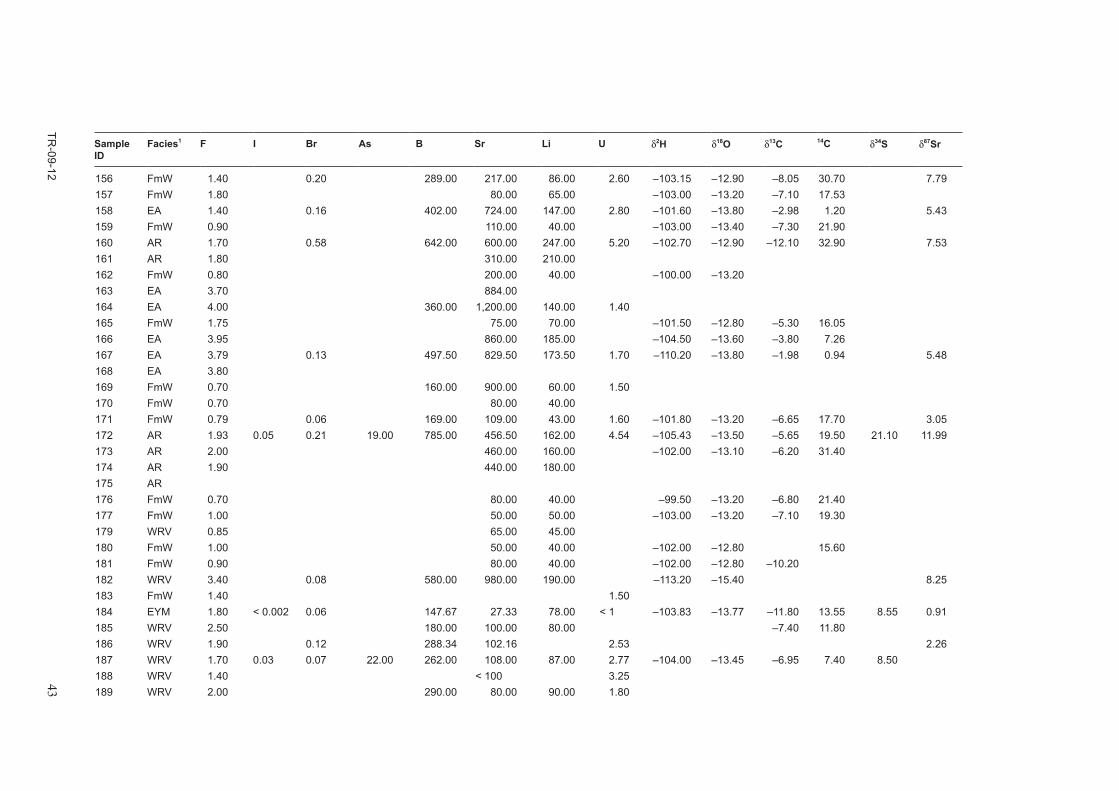
TR-09-12

43

Sample ID


156 FmW 1.40 0.20 289.00 217.00 86.00 2.60 –103.15 –12.90 –8.05 30.70 7.79157 FmW 1.80 80.00 65.00 –103.00 –13.20 –7.10 17.53158 EA 1.40 0.16 402.00 724.00 147.00 2.80 –101.60 –13.80 –2.98 1.20 5.43159 FmW 0.90 110.00 40.00 –103.00 –13.40 –7.30 21.90160 AR 1.70 0.58 642.00 600.00 247.00 5.20 –102.70 –12.90 –12.10 32.90 7.53161 AR 1.80 310.00 210.00162 FmW 0.80 200.00 40.00 –100.00 –13.20163 EA 3.70 884.00164 EA 4.00 360.00 1,200.00 140.00 1.40165 FmW 1.75 75.00 70.00 –101.50 –12.80 –5.30 16.05166 EA 3.95 860.00 185.00 –104.50 –13.60 –3.80 7.26167 EA 3.79 0.13 497.50 829.50 173.50 1.70 –110.20 –13.80 –1.98 0.94 5.48168 EA 3.80169 FmW 0.70 160.00 900.00 60.00 1.50170 FmW 0.70 80.00 40.00171 FmW 0.79 0.06 169.00 109.00 43.00 1.60 –101.80 –13.20 –6.65 17.70 3.05172 AR 1.93 0.05 0.21 19.00 785.00 456.50 162.00 4.54 –105.43 –13.50 –5.65 19.50 21.10 11.99173 AR 2.00 460.00 160.00 –102.00 –13.10 –6.20 31.40174 AR 1.90 440.00 180.00175 AR176 FmW 0.70 80.00 40.00 –99.50 –13.20 –6.80 21.40177 FmW 1.00 50.00 50.00 –103.00 –13.20 –7.10 19.30179 WRV 0.85 65.00 45.00180 FmW 1.00 50.00 40.00 –102.00 –12.80 15.60181 FmW 0.90 80.00 40.00 –102.00 –12.80 –10.20182 WRV 3.40 0.08 580.00 980.00 190.00 –113.20 –15.40 8.25183 FmW 1.40 1.50184 EYM 1.80 < 0.002 0.06 147.67 27.33 78.00 < 1 –103.83 –13.77 –11.80 13.55 8.55 0.91185 WRV 2.50 180.00 100.00 80.00 –7.40 11.80186 WRV 1.90 0.12 288.34 102.16 2.53 2.26187 WRV 1.70 0.03 0.07 22.00 262.00 108.00 87.00 2.77 –104.00 –13.45 –6.95 7.40 8.50188 WRV 1.40 < 100 3.25189 WRV 2.00 290.00 80.00 90.00 1.80

44 TR

-09-12

Sample ID


190 WRV 0.83 0.12 185.00 144.00 59.00 1.20 –106.35 –13.10 –9.05 8.84 0.75191 WRV 1.21 0.01 0.15 8.30 127.88 66.38 49.38 0.80 –100.25 –13.21 –10.49 23.10 8.79 0.48192 WRV 1.20 0.01 0.08 145.00 88.00 55.00 < 1 –107.00 –13.50 –12.65 8.30 1.04193 WRV 1.70 0.01 0.04 159.00 40.00 47.00 < 1 –111.00 –13.80 –10.15 9.20 1.34194 WRV 1.70 < 0.002 0.04 166.00 36.00 50.00 < 1 –107.00 –13.90 –10.50 13.50 9.20 1.47195 WRV 1.60 0.01 0.03 155.00 32.00 39.00 M –107.50 –13.90 –9.45 18.20 9.90 1.59196 WRV 1.70 < 0.002 0.04 38.00 105.00 34.00 35.00 0.57 –106.00 –13.80 –9.90 8.70 9.50 1.27197 FmW 1.60 < 0.002 0.05 154.00 53.00 42.00 1.00 –104.00 –14.10 –8.30 23.50 11.90 3.40198 FmW 1.40 < 0.002 0.05 5.80 175.00 66.00 44.00 0.49 –98.00 –13.10 –9.45 22.40 9.30199 EYM 2.25 < 0.002 0.06 193.50 50.50 81.00 3.00 –106.38 –13.80 –6.25 12.40 13.15 4.54200 WRV 0.90 0.11 0.16 698.00 322.00 178.00 < 1 –108.00 –13.25 –2.55 3.60 16.30 4.40201 WRV 1.20 0.08 0.18 650.00 204.00 147.00 M –106.00 –13.50 –0.50 4.30 20.70202 EYM 2.20 < 0.002 0.05 177.17 3.33 129.33 2.00 –105.50 –13.80 –7.57 12.40 9.05 2.05203 EYM 2.20 < 0.002 0.05 182.50 7.50 117.50 2.00 –108.75 –13.75 –7.10 12.35 10.65 2.59204 EYM 2.20 0.01 0.05 162.00 5.00 130.00 2.00 –108.00 –13.90 –6.80 19.90 9.80 2.38205 EYM 1.80 < 0.002 0.05 166.00 25.00 93.00 1.00 –110.00 –13.80 –7.10 15.20 10.40 2.82206 EYM 2.00 0.16 15.00 163.00 34.00 84.00 1.00 –107.50 –13.85 –7.65 10.30 2.92207 EYM 1.90 0.01 0.11 147.50 62.00 53.00 M 105.25 –13.80 –7.80 19.40 10.90208 EYM 1.65 < 0.002 0.04 157.00 36.00 68.00 1.00 –104.00 –13.60 –7.60 21.00 10.60 2.77209 EYM 2.00 < 0.002 0.04 190.00 3.00 126.00 2.00 –106.25 –13.55 –6.60 12.50 10.90 1.44210 EYM 2.60 < 0.002 0.04 185.00 2.00 132.00 2.00 –110.40 –13.95 –6.40 12.60 11.65 2.14211 EYM 2.20 < 0.002 0.05 186.00 1.10 145.00 2.56 –106.00 –13.20 –7.10 9.20 9.60 1.48212 EYM 1.75 < 0.002 0.05 1.40 138.00 58.50 42.00 0.77 –101.75 –13.53 –8.68 22.95 11.50 3.06213 EYM 2.00 < 0.002 0.06 185.00 8.00 114.00 1.71 –104.50 –13.40 –8.50 9.30 2.28214 EYM 2.12 < 0.002 0.05 31.00 134.67 1.87 137.67 1.95 –105.00 –13.75 –7.33 8.40 11.05 1.61215 EYM 2.40 < 0.002 0.05 160.00 1.09 132.00 1.44 –101.50 –12.10 –7.45 9.00 11.20 0.98216 EYM 2.10 < 0.002 0.07 186.50 1.88 133.00 1.79 –103.00 –13.00 –7.00 11.40 9.80 1.74217 EYM 2.10 < 0.002 0.08 151.00 16.90 98.20 1.95 –100.00 –11.75 –9.50 14.90 9.20 2.10218 EYM 2.05 < 0.002 0.05 30.00 137.00 16.87 116.33 2.06 –103.00 –13.25 –7.48 12.50 9.80 0.62219 EYM 1.95 < 0.002 0.06 172.00 9.60 109.00 1.69 –102.63 –13.20 –8.49 8.70 2.79220 EYM 1.80 < 0.002 0.05 14.00 173.00 35.00 86.00 2.33 –102.00 –13.40 –6.80 12.00 9.80221 EYM 2.00 0.01 0.06 8.40 154.00 75.00 47.00 1.52 –100.00 –13.20 –8.35 22.10 8.00224 WYM 4.18 0.02 0.05 289.67 4.00 266.83 10.00 –106.00 –14.13 –5.10 8.40 9.82 2.14

TR-09-12

45

Sample ID


225 WYM 2.95 0.01 0.06 234.00 2.50 180.00 3.00 –104.75 –14.25 –8.38 21.50 10.85 1.53226 WYM 2.87 0.01 0.05 237.33 1.33 161.67 2.00 –105.83 –14.40 –6.83 10.00 11.17 1.47227 EYM 1.94 0.01 0.04 9.25 137.00 66.00 46.50 0.95 –101.00 –13.40 –8.26 21.20 10.80 1.84228 EYM 2.47 0.07 110.00 68.00 2.50 –102.00 –13.65 4.22230 WRV 1.30 0.01 0.09 238.00 62.90 51.50 4.32 –104.00 –13.10 –9.85 22.60 –0.07231 WRV 1.10 < 0.002 0.08 18.00 171.00 137.00 57.00 2.99 –104.50 –13.50 –11.30 20.70 2.10 0.44232 WRV 1.40 0.06 0.10 13.00 275.00 131.00 58.00 5.85 –101.00 –13.10 –10.55 24.40 5.05 1.80233 BM 4.11 0.01 0.08 8.25 341.50 306.17 320.67 1.06 –102.08 –13.58 –3.40 4.70 16.23 8.98234 BM 3.99 0.01 0.11 5.40 321.67 298.67 288.00 1.01 –100.67 –13.60 –3.60 4.75 16.23 7.59235 BM 0.95 < 0.002 0.09 213.50 461.50 77.50 9.00 –101.75 –13.40 –5.25 9.00 14.70 5.09236 SECF 2.15 < 0.002 0.07 183.25 146.75 78.00 4.25 –104.90 –13.85 –6.53 11.70 13.43 4.66237 SECF 2.04 < 0.002 0.07 11.00 178.00 146.63 79.75 4.99 –104.73 –14.05 –6.39 11.00 16.40 4.74238 SECF 2.03 0.01 0.07 11.00 180.00 143.50 76.00 4.41 –104.17 –14.00 –6.23 10.90 14.40 4.64239 SECF 2.01 0.01 0.05 11.00 178.63 146.50 74.88 4.74 –104.67 –14.07 –6.70 11.40 13.90 4.52240 SECF 2.01 0.01 0.05 9.20 184.50 132.25 77.50 4.52 –104.00 –14.07 –6.80 12.20 14.17 4.63241 FmW 1.00 0.01 0.04 6.20 150.50 76.30 41.95 0.84 –98.50 –12.95 –8.28 20.80 8.90 1.73242 FmW 1.10 0.01 0.05 3.90 154.00 91.25 36.70 0.72 –98.75 –13.10 –8.15 20.60 9.90 1.75243 FmW 1.70 0.01 0.05 4.90 144.25 72.38 36.80 0.53 –98.75 –13.10 –7.88 21.05 9.88 1.79244 FmW 1.70 < 0.002 0.05 5.80 146.50 60.15 37.75 0.44 –99.00 –13.10 –9.15 24.10 9.25 2.44245 FmW 0.88 < 0.002 0.05 7.20 123.50 77.00 37.50 1.52 –97.50 –13.10 –10.70 22.30 8.15 2.21246 FmW 1.05 < 0.002 0.05 4.55 124.75 95.20 35.60 1.09 –97.75 –13.14 –9.57 20.80 8.77 1.79247 FmW 1.60 < 0.002 0.05 5.40 131.00 67.30 35.35 0.53 –97.50 –13.30 –10.00 22.50 9.50 2.01248 FmW 1.95 < 0.002 0.05 6.20 123.50 64.00 36.90 0.79 –99.25 –13.10 –10.60 25.00 8.40 2.13249 EYM 2.11 0.01 0.04 4.90 149.00 55.50 54.00 0.95 –104.00 –13.65 –7.65 17.60 12.10 1.85250 WYM 2.17 0.01 0.04 14.50 193.00 27.50 62.50 4.02 –102.25 –13.55 –11.30 16.45 9.38 0.49251 BM 6.67 0.03 0.03 10.00 844.00 1,550.00 649.00 < 0.06 –105.00 –14.10 –1.80 27.50252 BM 0.60 < 0.002 0.08 216.00 557.00 72.50 8.00 –100.00 –13.88 –5.65 6.40 14.60 5.19253 BM 0.56 0.01 0.09 5.25 204.80 550.75 67.63 7.24 –101.00 –13.67 –5.44 7.05 15.13 5.19254 BM 0.59 < 0.002 0.09 5.70 208.00 583.00 69.00 8.71 –101.67 –13.53 –5.60 7.65 14.70 5.04255 BM 0.70 0.04 0.12 212.50 509.50 73.50 5.00 –101.30 –13.53 –4.50 14.60 5.08256 BM 6.50 0.03 0.12 942.00 967.00 647.00 < 1 –107.50 –13.80 –2.00 2.50 27.60 5.31258 WYM 2.80 0.01 0.06 10.00 154.00 7.40 69.00 3.85 –99.50 –13.60 –8.50 17.60 4.70 –0.36259 BM 0.82 0.02 0.09 1.25 234.50 352.00 122.00 0.20 –97.75 –13.40 –5.70 7.25 21.65 4.33

46 TR

-09-12

Sample ID


260 BM 0.81 0.02 0.17 2.00 247.00 497.50 106.00 2.89 –98.00 –13.25 –4.80 6.40 16.10 5.15261 BM 0.86 0.01 0.10 < 1.2 246.50 488.00 108.00 5.29 –98.50 –13.30 –4.70 5.75 14.25 5.93262 BM 0.89 0.01 0.10 < 1.2 241.50 482.00 136.50 5.25 –98.75 –13.30 –4.80 5.80 14.30 5.89263 BM 0.95 0.01 0.11 273.00 630.00 116.00 6.00 –98.00 –13.00 –4.85 8.40 14.30 5.66264 BM 0.90 0.01 0.15 283.00 560.50 115.00 5.50 –99.88 –13.50 –4.90 6.50 13.30265 FmW 2.05 0.01 0.06 10.00 108.00 54.95 39.05 0.87 –97.25 –13.15 –8.40 25.30 9.20 1.99266 FmW 2.05 0.01 0.06 9.30 118.50 61.65 35.75 0.69 –99.50 –13.10 –9.10 24.95 9.85 2.35267 FmW 2.05 < 0.002 0.05 10.00 133.50 62.30 37.50 0.90 –96.75 –13.15 –10.05 24.80 9.70 2.23268 FmW 2.10 < 0.002 0.05 11.00 121.50 61.25 39.10 0.88 –98.50 –13.10 –10.20 25.70 9.55 2.06269 FmW 1.90 < 0.002 0.07 142.00 53.10 41.30 0.65 –100.00 –12.70 –8.75 26.20 9.70 2.93270 WYM 3.51 0.02 0.05 12.50 216.00 41.00 92.50 4.29 –102.00 –13.65 –7.00 12.90 11.30 0.70272 SECF 0.94 0.00 12.00 209.00 373.00 52.00 4.78273 EYM 2.60 0.01 0.05 6.70 150.00 25.20 63.15 2.54 –102.25 –13.65 –8.13 21.75 12.20 2.22274 FmW 1.60 0.05 37.17 1.30 –97.25 –13.17 –8.60 30.70 3.00275 SW 0.05 < 0.002 0.01 0.50 31.00 5.00276 AR 3.30 0.01 0.33 550.00 369.50 250.00 6.70 –108.25 –14.23 –6.60 26.20 20.10 3.86277 AR 3.70 0.02 0.31 496.67 363.33 256.67 8.00 –107.00 –14.03 –5.90 28.80278 AR 3.60 0.02 0.31 500.00 350.00 240.00 –105.00 –14.00 3.89279 AR 3.10 0.01 0.29 640.00 440.00 180.00 –104.00 –13.91 –7.80 13.80280 AR 3.70 0.01 0.35 610.00 350.00 230.00 –104.00 –13.89 –6.50 17.10281 FmW 1.83 0.06 9.80 115.57 47.19 37.71 0.74 –96.50 –12.95 –7.88 30.80 3.52282 AR 4.00 0.02 0.32 410.00 410.00 240.00 –106.50 –13.95 3.33283 AR 3.10 < 0.002 0.31 610.00 380.00 240.00 –104.00 –13.99 –6.70 25.00284 AR 2.50 0.02 0.24 610.00 690.00 280.00 –105.00 –13.80 1.30285 P286 AR 4.05 0.06 0.30 592.00 405.50 263.00 8.00 –108.25 –14.00 –6.20 14.70 21.80 3.90287 AR 4.18 0.01 0.30 649.75 342.13 127.63 5.00 –106.50 –14.18 –8.25 17.93 19.60 3.99288 P 0.05 0.01 2.00289 EYM 2.98 < 0.002 0.08 25.00 59.93 1.98 –102.50 –13.69 –7.07 11.40 1.01290 P 0.05 0.01 8.00 0.50 2.00 0.50 –56.75 –7.50 1.22291 JaF 1.11 0.02 0.02 1,410.00 264.00 43.00 2.40 –105.00 –13.45 –11.00 12.30 8.80 0.21293 SECF 2.64 < 0.002 0.06 174.50 62.30 86.20 3.26 –106.67 –14.03 –7.22 12.77 12.95 2.57294 SW 0.30 < 0.002 0.01 3.00 86.00 17.00

TR-09-12

47

Sample ID


295 EYM 2.32 0.05 120.44 32.43 48.07 0.50 –101.76 –13.36 –8.47 22.25 10.81 2.12296 BM 1.12 < 0.002 0.10 204.00 567.00 88.67 6.13 –102.00 –13.80 –4.80 7.00 14.70 5.36297 EYM 2.00 0.21 115.34 46.73 70.09 0.50 –100.84 –13.53 –8.24 17.50 10.67 4.26298 WYM 3.70 < 0.002 0.16 4.00 86.00 –103.00 –13.82 –6.08 7.32 1.18299 FmW 2.35 0.06 116.00 59.66 47.79 0.63 –95.61 –12.73 –8.03 30.67 10.45 3.03301 SW 0.20 0.01 0.01 2.00 100.00 7.00302 SW 0.05 < 0.002 0.01 0.50 34.00 6.00303 SW 0.30 < 0.002 0.01 2.00 66.00 14.00304 SW 0.30 0.01 0.20 87.00 74.00 10.00 0.50 –82.50 –11.30 –13.15305 WYM 0.21 150.00 –13.95 –9.01 1.51306 WYM 4.90 490.00 310.00 –107.00 –13.80 –2.80307 EYM 4.70 450.00 590.00 –106.00 –13.80 –2.20 2.30 3.59308 WYM 5.50 0.01 0.18 1.00 220.00 –101.00 –13.90 –4.90 10.50309 EYM 2.05 < 0.002 0.04 45.00 93.00 –100.50 –13.40 –7.00 15.95310 EYM 2.12 0.08 0.04 122.02 22.35 126.47 1.99 –102.15 –13.90 –9.25 11.65 10.90 0.72311 EYM 2.11 0.01 0.18 110.70 53.39 82.98 1.11 –99.64 –13.39 –6.94 16.18 0.85312 EYM 1.97 0.05 22.37 73.77 –101.30 –13.45 –8.01 14.45 10.80 0.58313 EYM 2.15 < 0.002 0.03 34.50 143.33 –102.00 –13.50 –7.10 15.00314 EYM 2.00 < 0.002 0.05 44.00 110.00 –103.00 –13.50 –7.50 15.70315 PW 30.00 20.00 –99.78 –13.33 –9.48 28.33 3.29316 EYM 120.00 280.00 84.00 2.04317 EYM 4.60 27.00 130.00 –104.00 –14.00 –7.40 11.80318 EYM 1.80 0.45 50.00 –97.50 –12.75 –12.70 24.10319 WYM 4.59 < 0.002 0.06 203.80 0.50 64.33 4.50 –105.30 –14.37 –9.42 15.01 12.60 2.87320 WYM 4.43 6.33 72.00 –106.00 –13.93 –7.30 12.90321 SW 0.20 0.01 160.00 9.00 3.27324 EYM 1.60 42.50 170.00 –100.25 –13.45 –9.50 17.80325 EYM 2.50 17.00 67.00 –103.00 –13.80 –9.10 22.00326 EYM 0.06 550.00 –97.50 –13.20 –11.80 21.60327 WYM 1.40 6.50 66.50 –102.00 –13.60 –10.30 19.80329 SW 0.20 0.01 200.00 19.00330 SW 0.05 160.90 9.60 3.33331 SW 0.05 184.60 12.10 3.33

48 TR

-09-12

Sample ID


332 EYM 1.10 12.50 40.00 –102.00 –13.45 –11.40 21.90333 SW 0.20 45.00 10.00334 SW 0.20 0.01 44.00 2.00 3.75335 SW 0.05 54.40 5.20336 PW 0.45 0.26 –89.57 –11.63 2.45337 EYM 6.51 0.08 2.10 129.06 –100.48 –14.00 –12.83 22.88 11.40 0.73338 PW 0.70 250.00 20.00 –97.35 –13.40 –9.85 27.20 4.38340 EYM 0.92 0.05 1.47 39.90 –101.05 –13.20 –10.70 27.34 1.77341 PW 0.75 0.04 0.53 148.65 36.00 –99.98 –13.47 –11.28 30.49 10.85 4.07343 SW 0.20 0.01 97.00 10.00 3.68344 EYM 1.03 0.01 0.05 116.67 10.40 45.87 1.30 –98.93 –13.30 –11.25 20.45 2.12345 PW 0.22 0.02 110.95 10.11 2.00 0.50 –73.10 –9.90 3.70350 P354 PW 22.97 4.31 –89.50 –12.40 3.71355 P357 SW 0.05 0.01 89.00 8.00 3.46359 FmW –90.60 –12.57 –11.00 75.70 2.65360 FmW 0.95 0.10 36.00 105.00 –92.50 –12.73 –12.00 65.07 1.94361 SW 0.30 0.01 23.00 2.00 3.50363 P364 P426 P427 P428 SW 0.05 80.00 9.00443 P444 P1 See Table 2-4 for hydrofacies’ abbreviations.

TR-09-12 49

The 254 groundwater samples contained in the raw dataset have been grouped into 10 “hydrofacies” by geographical and/or chemical similitude (Oliver and Patterson 2002), although the groupings are not intended to be either rigorous or comprehensive. The 10 hydrofacies of the groundwater samples, together with the four other water types (perched waters, pore waters, surface waters, and precipitation) gives a total of 14 different “categories” of water samples. Each water category has been given a different colour, a different symbol type and a different abbreviation, which is maintained throughout the report. 0 collects the colour code, symbol type and abbreviation for each category and Figure 2-1 shows the general distribution of the samples of each water category on a shaded relief map. We will call hydrofacies to each category, even recognising that we are using the term “hydrofacies” in a broad sense.

Table 2-4. Hydrofacies used in this report. The colour code, symbol type, and abbreviations used throughout the report are included.

Hydrofacies Water type Colour code Symbol Abbreviation

Amargosa River Groundwater AREastern Yucca Mountain Groundwater EYMFortymile Wash Groundwater FmWBare Mountain Groundwater BMEastern Amargosa Groundwater EAAsh Meadows Groundwater AMWestern Yucca Mountain Groundwater WYMWestern Rock Valley Groundwater WRVSouth East Crater Flats Groundwater SECFJackass Flat Groundwater JAFPerched Water Perched water PWSurface Water Surface water SWPrecipitation Precipitation PPore Water Pore water PW

Figure 2-1. Map with the location of the samples of the raw dataset. The left-hand map plots the ground-water samples (all 10 hydrofacies), and the map on the right plots the non-groundwater samples (perched waters, surface waters, pore waters and precipitation). The red polygon marks the boundary of the Nevada Test Site.

50 TR-09-12

2.3 Water typesThe following five water types can be identified in the Yucca Mountain area:

Precipitation. This is the starting point for all water types. Evapotranspiration of precipitation waters in the soil zone appears to be a very important process in the control of vadose zone pore waters, perched waters and saturated zone ground water compositions in this area (Meijer 2002).

Surface waters. Surface waters in these desert areas are short-lived and ephemeral. Cl concentrations are higher relative to precipitation, indicating that they have either dissolved Cl-bearing solids and/or that they have experienced evapo-transpiration, although the former interpretation seems more plausible. The fact that SO4 to Cl ratios in these samples are similar to the precipitation samples suggests also dissolution of SO4-bearing solids and/or evapo-transpiration. The elevated HCO3 to Cl ratios in these samples strongly suggest that CO3-bearing solids have also been dissolved by these surface waters (Meijer 2002). Silica has very low concentrations in precipitation samples (< 1.0 mg/l). However, surface waters show concentrations of up to 37 mgL–1 with an average value of approximately 25 mg L–1. Given that the age of surface waters is in the range of hours to days, these data indicate there is a very soluble form of silica in surface soils that is rapidly dissolved by surface waters.

Pore waters. These are waters extracted from the unsaturated zone (volcanic tuffs) in the Yucca Mountain area. Extraction was performed by either uniaxial/triaxial compression or ultra-centrifugation. Pore waters have ratios of Ca, Na, HCO3 and SO4 to Cl that are all lower than those found in precipitation. The lower ratios probably reflect the precipitation of alkaline earth carbonates and possibly sulphates in the soil zone (Meijer 2002). Downward matrix flow in the unsaturated zone is indicated by ion exchange within zeolitised layers. The upper portions of these layers have gained Sr, Mg, and Ca from percolating water and lost Na, K and Rb. The fact that this exchange is most pronounced at the tops of zeolitised layers and absent in stratigraphically lower zeolitised layers when multiple layers exist provides strong evidence of downward percolation of water (Stuckless and Dudley 2002).

Perched waters. Perched waters are groundwaters in perched aquifers or aquitards above the main water table. They are chemically more diluted than the pore waters, but appear to have gained their solutes by similar mechanisms. Sulphates were dissolved in the soil zone in addition to carbonates and chlorides. The dissolution of the less soluble phases (i.e. alkaline earth carbonates and sulphates) in the soil zone implies that perched waters were infiltrated under wetter climatic conditions (Meijer 2002).

Groundwaters. Saturated zone groundwaters originated by processes similar to those that formed the perched groundwaters, except that the former were subject to more extensive ion exchange reactions. Groundwaters in the shallow saturated zone beneath Yucca Mountain appear to include a significant component that was locally infiltrated. Deeper saturated zone waters probably infiltrated further upgradient in the direction of Pahute Mesa (Meijer 2002). Two main facies have been recognised: (1) pH-neutral, Na+Ca+Mg+SO4+HCO3 water with moderate to high total-dissolved solids; and (2) alkaline, Na+HCO3+CO3 water with high total dissolved solids.

2.4 Exploratory analysisThe aim of the exploratory analysis is twofold: (1) to assess the global relationships between all the water categories and (2) to screen the dataset for outliers, both on a total system basis and on a hydro-facies basis. The first part of the exploratory analysis defines the basic compositional characteristics of the whole dataset, the main hydrochemical trends and the compositional range of the most important chemical variables. The outcome of this analysis gives a distinction between conservative and non-conservative variables and a first identification of samples with extreme chemical signatures (outliers). The total-system exploratory analysis is carried out by means of ion-ion plots and Principal Components Analysis (PCA).

The second part of the exploratory analysis is performed on a hydrofacies basis. Each hydrofacies is treated separately and its behaviour compared with that of other hydrofacies. This permits the identi-fication of samples strongly affected by non-mixing processes (evaporation, water-rock interaction, ion exchange, etc) and the preliminary selection of potential end-member waters.

TR-09-12 51

2.4.1 Total-system exploratory analysisPiper diagrams and box-and-whiskers plotsThe Piper diagram in Figure 2-2 provides an immediate grasp of the general chemistry and trends in the raw dataset. In Figure 2-2, samples are colour-coded by hydrofacies and symbol size is propor-tional to Total Dissolved Solids (TDS, in mgL–1). Most waters are low-TDS of a sodium-bicarbonate type, although exceptions to this rule do exist. The most obvious ones are: (1) the calcium-sodium bicarbonate-sulphate waters from the Bare Mountain (cyan; medium-TDS) and Ash Meadows (orange; high-TDS) hydrofacies; (2) the calcium-magnesium bicarbonate waters that include both precipitation (grey) and surface waters (yellow), both very low-TDS; and (3) the calcium-magnesium sulphate-chloride signature of some, generally low-TDS pore waters (black). Minimum TDS is 0.061 meqL–1 (2.78 mgL–1) and maximum TDS is 108.2 meqL–1 (3968.4 mgL–1), with a mean value for the whole dataset of 12.4 meqL–1 (470.1 mgL–1) and a median value of 9.1 meqL–1. (368.0 mgL–1)

Several trends are also apparent: (1) pore waters have a very broad compositional range, from a pure sodium bicarbonate type to a calcium-magnesium sulphate-chloride type; (2) the Bare Mountain hydro-facies waters are also quite variable, defining a trend from a sodium bicarbonate type to a calcium-magnesium bicarbonate-sulphate type; and (3) the Ash Meadows hydrofacies waters follow a similar trend but even more pronounced, extending to the calcium-magnesium sulphate (-chloride) type.

In order to gain a general idea of the concentration range for the major ions, minor ions and isotopes, box-and-whiskers plots are very suitable. In the box-and-whiskers plots that follow Figures 2-3, 2-4 and 2-5, the box has the 75th and 25th percentiles as its upper and lower limits, and the middle line represents the median of the distribution (50th percentile), while the whiskers mark the 95th and 5th percentiles. In addition, the square is the mean, crosses are the 99th and 1st percentiles, and the horizontal bars are the maximum and minimum values.

Figure 2-2. Piper diagrams for the raw dataset, including all water categories. Symbol size is proportional to the Total Dissolved Content of the sample, expressed in mmolL–1. As stated in the legend, the lowest TDS is 0.061 meqL–1 (2.78 mgL–1) and the highest 108.225 meqL–1 (3968.4 mgL–1).

Ca2+

CATIONS

Mg

2+ Na ++

K + CO3

2- +HC

O 3-

SO4 2-

Cl-

ANIONS

SO4

2- +Cl

- Ca 2++

Mg 2+

EXPLANATIONAmarosa RiverEastern Yucca MountainFortymile WashBare MountainsEastern AmargosaAsh MeadowsWestern Yucca MountainWestern Rock ValleySouth East Crater FlatsJackass FlatsPerched WaterSurface WatersPrecipitationPore Waters

0.061108.225

52 TR-09-12

Figure 2-3 plots the relevant statistics for the major ions and Table 2-5 gives their numerical values. As already mentioned, concentrations of the major ions are generally low. Bicarbonate is the princi-pal anion, with a median value of 162 mgL–1 (mean value = 200.3 mgL–1), followed by sulphate and then chloride. Sodium is the principal cation (median = 67.3 mgL–1; mean = 80.8 mgL–1), followed by calcium, potassium and magnesium. All the distributions are skewed to the right (i.e. the median value is smaller than the mean value, and the coefficient of variation (standard deviation divided by the mean value) is considerably larger for sulphate, chloride and magnesium than for the other major ions (Table 2-5). Bicarbonate has the lowest coefficient of variation, indicating that the dispersion of values around the mean is smaller than for the other ions.

As regards the minor and trace elements (Figure 2-4), the most abundant of them is fluoride (median value=1,700μgL–1,meanvalue=1,996μgL–1; 365 samples), followed by boron (165 samples), strontium (268 samples), lithium (249 samples) and bromide (188 samples), all of them with median concentrationvaluesoftheorderof100μgL–1. Finally, arsenic (54 samples), iodine (106 samples) anduranium(136samples)havemedianconcentrationsbetween2and9μgL–1.

Ca Mg Na K Cl HCO3 SO4 NO3

0.1

1

10

100

1000

Con

cent

ratio

n (m

g/L)

Major ions

Figure 2-3. Box-and-whiskers plot for the major ions in the raw dataset. Concentrations are expressed in mgL–1. Box: 75th and 25th percentiles; middle line: median (50th percentile); whiskers: 95th and 5th percentiles; square: mean; crosses: 99th and 1st percentiles; horizontal bars: maximum and minimum values.

Table 2-5. Basic statistics for the main ions in the raw dataset.

Species Mean Standard dev Coeff of var P25 P75 Median

Ca 26.3 25.2 0.96 7.05 44 19Mg 6.92 10.5 1.52 0.304 9.9 2.121Na 80.76 100.6 1.25 42 102 67.295K 7.47 7.95 1.06 3.51 9.1 6.15Cl 24.5 37.5 1.53 6.4 26.2 11.4HCO3 200.3 164.4 0.82 127.5 263 162SO4 67.4 104.5 1.55 15.3 92.17 28.835NO3 7.31 9.62 1.31 1.42 8.12 4.61

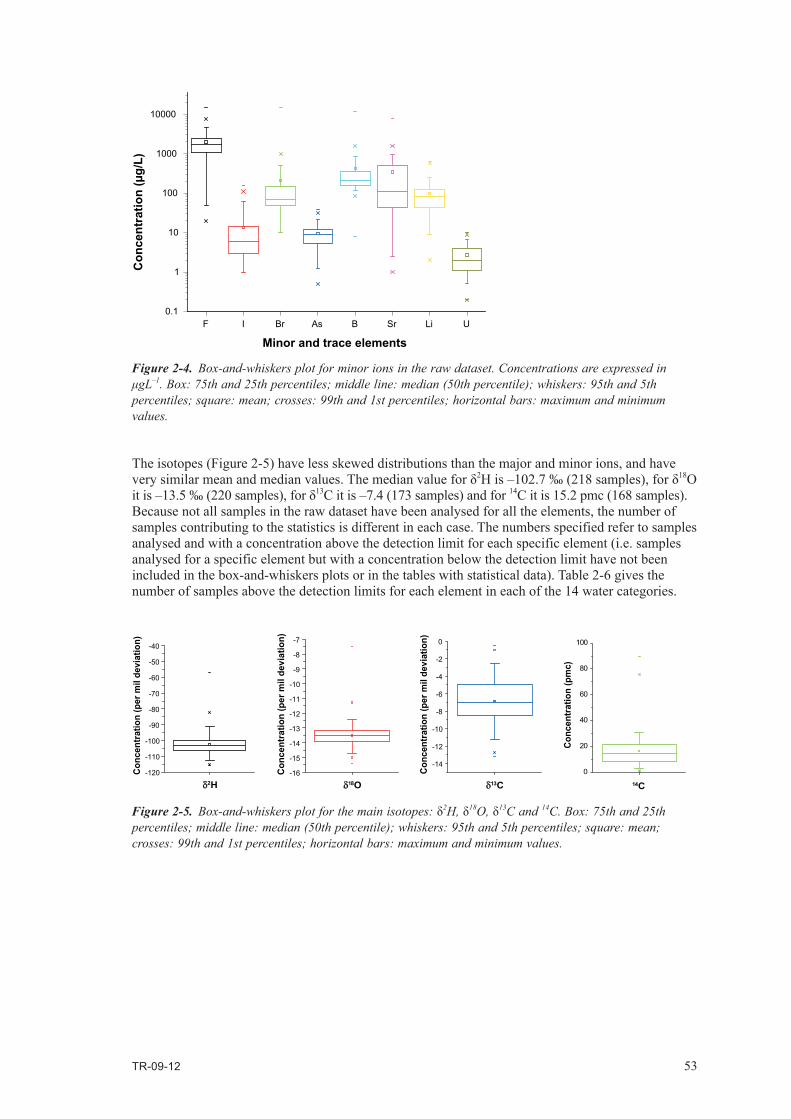
TR-09-12 53

The isotopes (Figure 2-5) have less skewed distributions than the major and minor ions, and have verysimilarmeanandmedianvalues.Themedianvalueforδ2His–102.7‰(218samples),forδ18O itis–13.5‰(220samples),forδ13C it is –7.4 (173 samples) and for 14C it is 15.2 pmc (168 samples). Because not all samples in the raw dataset have been analysed for all the elements, the number of samples contributing to the statistics is different in each case. The numbers specified refer to samples analysed and with a concentration above the detection limit for each specific element (i.e. samples analysed for a specific element but with a concentration below the detection limit have not been included in the box-and-whiskers plots or in the tables with statistical data). Table 2-6 gives the number of samples above the detection limits for each element in each of the 14 water categories.

Figure 2-4. Box-and-whiskers plot for minor ions in the raw dataset. Concentrations are expressed in μgL–1. Box: 75th and 25th percentiles; middle line: median (50th percentile); whiskers: 95th and 5th percentiles; square: mean; crosses: 99th and 1st percentiles; horizontal bars: maximum and minimum values.

F I Br As B Sr Li U0.1

1

10

100

1000

10000

Minor and trace elements

Con

cent

ratio

n (µ

g/L)

-120

-110

-100

-90

-80

-70

-60

-50

-40

Conc

entra

tion

(per

mil

devi

atio

n)

-16

-15

-14

-13

-12

-11

-10

-9

-8

-7

Con

cent

ratio

n (p

er m

il de

viat

ion)

-14

-12

-10

-8

-6

-4

-2

0

Conc

entra

tion

(per

mil

devi

atio

n)

0

20

40

60

80

100

Conc

entra

tion

(pm

c)

δ18O 14Cδ2H δ13C

Figure 2-5. Box-and-whiskers plot for the main isotopes: δ2H, δ18O, δ13C and 14C. Box: 75th and 25th percentiles; middle line: median (50th percentile); whiskers: 95th and 5th percentiles; square: mean; crosses: 99th and 1st percentiles; horizontal bars: maximum and minimum values.

54 TR-09-12

Table 2-6. Number of samples above detection limit for each element, grouped by hydrofacies.

Element Water category TotalsAR1 EYM FmW BM EA AM WYM WRV SECF JaF PW SW P PrW

Ca 28 46 55 16 20 49 13 19 7 1 6 17 39 81 397Mg 28 46 55 16 20 49 13 19 7 1 6 17 39 81 397Na 28 46 55 16 20 49 13 19 7 1 6 17 39 81 397K 28 46 55 16 20 49 13 19 7 1 6 17 39 81 397Cl 28 46 55 16 20 49 13 19 7 1 6 17 39 81 397HCO3 28 46 55 16 20 49 13 19 7 1 6 17 39 81 397SO4 28 46 55 16 20 49 13 19 7 1 6 17 39 81 397NO3 21 38 49 12 16 41 9 17 7 1 2 1 18 77 309SiO2 28 46 54 16 20 48 13 19 7 1 6 17 24 76 375NH4 5 13 12 9 7 7 5 4 5 1 1 1 2 0 72PO4 17 27 37 3 13 17 8 11 7 1 2 1 5 0 149F 26 44 53 16 20 45 12 19 7 1 4 17 23 78 365I 12 28 11 16 2 2 9 12 6 1 1 6 0 0 106Br 14 40 26 16 8 10 10 15 7 1 3 12 4 22 188As 2 8 14 7 2 3 3 5 5 0 0 5 0 0 54B 17 31 27 16 11 28 7 17 7 1 1 1 1 0 165Sr 26 44 49 16 19 39 12 18 7 1 5 17 15 0 268Li 22 46 48 16 15 40 13 17 7 1 5 17 2 0 249U 11 30 29 14 10 14 7 10 7 1 1 1 1 0 136d2H 16 45 46 16 12 14 12 14 6 1 6 1 29 0 218d18O 16 45 46 16 12 15 13 14 6 1 6 1 29 0 220d13C 13 44 37 16 11 14 13 14 6 1 3 1 0 0 17314C 12 41 43 14 10 15 11 12 6 1 3 0 0 0 1681See Table 2-4 for abbreviations.

Ion-ion plotsAlthough most combinations of chemical variables have been explored, only those depicting clearly the main trends, limiting values and outliers are included here. The chemical variables that have given the most valuable information in the Yucca Mountain system are: major ions (Ca, Na, K, Mg, SO4, Cl, HCO3), the Na/Cl ratio, stable isotopes (deuterium, 18O, and 13C) and 14C. Figure 2-6 to 2-9 plot the behaviour of the major ions and isotopes with respect to several compositional variables (chloride and bicarbonate in most cases, but also with respect to calcium, oxygen-18 and carbon-13) both in linear and logarithmic scales (in the latter case to better appreciate the low-concentration end). Chloride has been selected in most graphs as a tracer of “evolution” due to its conservative behaviour in most systems. Bicarbonate is also a good indicator of evolution in carbonate systems, although it is not necessarily a conservative element.

The word “trend” is used throughout the discussion that follows. It should be understood in a qualita-tive way, and not in its statistical sense (this is why the word “correlation” has not been used). In most cases the presence of a trend (meaning literally “following a general course” or “showing a tendency”) will be clear from the scattergram. In other cases, where more than one trend can be appreciated in a single scattergram, two copies of it are presented: a “clean” copy and an annotated one, where the trends (already visible in the “clean” copy) are visually enhanced by means of coloured lines or arrows to guide the reader in the discussion.

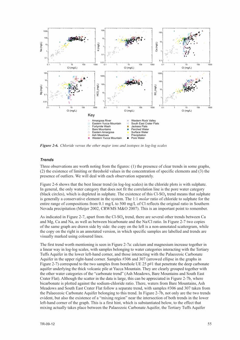
TR-09-12 55

TrendsThree observations are worth noting from the figures: (1) the presence of clear trends in some graphs, (2) the existence of limiting or threshold values in the concentration of specific elements and (3) the presence of outliers. We will deal with each observation separately.

Figure 2-6 shows that the best linear trend (in log-log scales) in the chloride plots is with sulphate. In general, the only water category that does not fit the correlation line is the pore water category (black circles), which is depleted in sulphate. The existence of this Cl-SO4 trend means that sulphate is generally a conservative element in the system. The 1:1 molar ratio of chloride to sulphate for the entire range of compositions from 0.1 mg/L to 500 mg/L of Cl reflects the original ratio in Southern Nevada precipitation (Meijer 2002, CRWMS M&O 2007). This is an important point to remember.

As indicated in Figure 2-7, apart from the Cl-SO4 trend, there are several other trends between Ca and Mg, Ca and Na, as well as between bicarbonate and the Na/Cl ratio. In Figure 2-7 two copies of the same graph are drawn side by side: the copy on the left is a non-annotated scattergram, while the copy on the right is an annotated version, in which specific samples are labelled and trends are visually marked using coloured lines.

The first trend worth mentioning is seen in Figure 2-7a: calcium and magnesium increase together in a linear way in log-log scales, with samples belonging to water categories interacting with the Tertiary Tuffs Aquifer in the lower left-hand corner, and those interacting with the Palaeozoic Carbonate Aquifer in the upper right-hand corner. Samples #306 and 307 (arrowed ellipse in the graphs in Figure 2-7) correspond to the two samples from borehole UE 25 p#1 that penetrate the deep carbonate aquifer underlying the thick volcanic pile at Yucca Mountain. They are clearly grouped together with the other water categories of the “carbonate trend” (Ash Meadows, Bare Mountains and South East Crater Flat). Although the scatter in the data is large, this can be appreciated in Figure 2-7b, where bicarbonate is plotted against the sodium-chloride ratio. There, waters from Bare Mountains, Ash Meadows and South East Crater Flat follow a separate trend, with samples #306 and 307 taken from the Palaeozoic Carbonate Aquifer belonging to this trend. In Figure 2-7b, not only are the two trends evident, but also the existence of a “mixing region” near the intersection of both trends in the lower left-hand corner of the graph. This is a first hint, which is substantiated below, to the effect that mixing actually takes place between the Palaeozoic Carbonate Aquifer, the Tertiary Tuffs Aquifer

Figure 2-6. Chloride versus the other major ions and isotopes in log-log scales

56 TR-09-12

and the Quaternary Basin-fill Aquifer. The Tertiary Tuffs Aquifer appears to evolve through a rapid increase in the Na/Cl ratio with HCO 3, while the Palaeozoic Carbonate Aquifer evolves through a very slow increase in the Na/Cl ratio. Here also, samples #306 and 307 concur well with the “Palaeozoic Carbonate Aquifer trend”, while all the other samples from the same water categories (belonging to the Eastern and Western Yucca Mountain hydrofacies) follow the “Tertiary Tuffs Aquifer trend”.

The last row of graphs in Figure 2-7 shows the behaviour of Ca and Na in log-normal scales. Clearly, surface waters and precipitation samples follow a separate trend from the rest of the water categories. It is interesting to note the existence of a “compositional gap” between the Na concentra-tion of the most concentrated surface waters (17 mg/L) and the Na concentration of the most diluted groundwaters of 35 mg/L (those from the Fortymile Wash hydrofacies). Only one perched water sample and one pore water occupy this compositional gap. This observation suggests that surface waters and precipitation do not play an important role (at the present time) in the main water budget of the Yucca Mountain area. On the other hand, the perched water samples seem to have continuity with the remainder of the groundwaters, occupying the position where the two trends followed by

Figure 2-7. Important trends in the raw dataset with respect to Mg, Ca, Na and bicarbonate. The graphs in the left-hand column are non-annotated, while their copies in the right-hand column are annotated. In this right-hand column, red trend arrows are drawn by eye and are not statistical fits. Ca and bicarbonate are always in the horizontal axis, while the vertical axis is occupied by Mg, Na or the Na/Cl relation. Note that the different axis scales for plots (a) are in log-log scales, for plots (b) they are in normal-normal scales and for plots (c) they are in log-normal scales.

TR-09-12 57

the groundwater samples converge (Figure 2-7c, right-hand graph). The behaviour of the two trends differs. In one, Na and Ca increase together, while in the other Na and Ca change inversely (there is a decrease in Na when Ca increases). This latter trend is followed by the Eastern and Western Yucca Mountain hydrofacies, both of which interact with the Tertiary Tuffs aquifer. It has been suggested (Vaniman et al. 2001, Meijer 2002) that cation exchange between these two ions is an important process in the volcanic rocks in the Yucca Mountain area, and this inverse trend could be evidence of the actuation of such a process. However, there are other potential explanations, and a mixing hypothesis is favoured when the Eastern and Western Yucca Mountain hydrofacies are treated in detail below.

The final trend analysed here is that of oxygen-18 versus deuterium. Figure 2-8a shows the entire range of delta values including precipitation samples, whereas part (b) zooms in on the central part, excluding most precipitation samples. In both graphs, the blue line marks the global meteoric water line (Craig 1961). In the graph on the right, two other parallel lines are plotted: the red line is a local palaeometeoric water line for southern Nevada (White and Chuma 1987), and the green line is the “evaporation line” in the sense that waters plotting to the right of this line are probably affected by evaporation (Thomas et al. 1996). In this graph we again have a hint as to the role that is possibly played by evaporation in the waters of the Yucca Mountain area.

Limiting and threshold valuesSeveral threshold values and limits are apparent in the raw dataset from a total-system perspective, as illustrated by Figure 2-9. Graph (a) shows how chloride in groundwaters has a minimum value of approximately 6 mgL–1, whereas graphs (b) and (c) point to a minimum value for bicarbonate in groundwaters of some 110 mgL–1. There are, of course, precipitation samples and surface water samples with lower Cl and HCO3 concentrations, but no groundwater samples seem to fall below this threshold. Figure 2-6 also shows clearly the chloride threshold for groundwaters when plotted against calcium and magnesium. The most reasonable way of interpreting these threshold values is by invoking the existence of end-member waters with extreme compositions, which upon mixing with other waters give a range of compositions limited by these threshold values. This hypothesis is further developed below.

Figure 2-8. Oxygen-18 versus deuterium plot. The graph on the left plots the complete range of values and the graph on the right only the central part, excluding most precipitation samples. The blue line is the global meteoric water line, the red line is a local palaeometeoric water line for southern Nevada and the green line marks the approximate location of waters affected by evaporation (to the right of the green line).

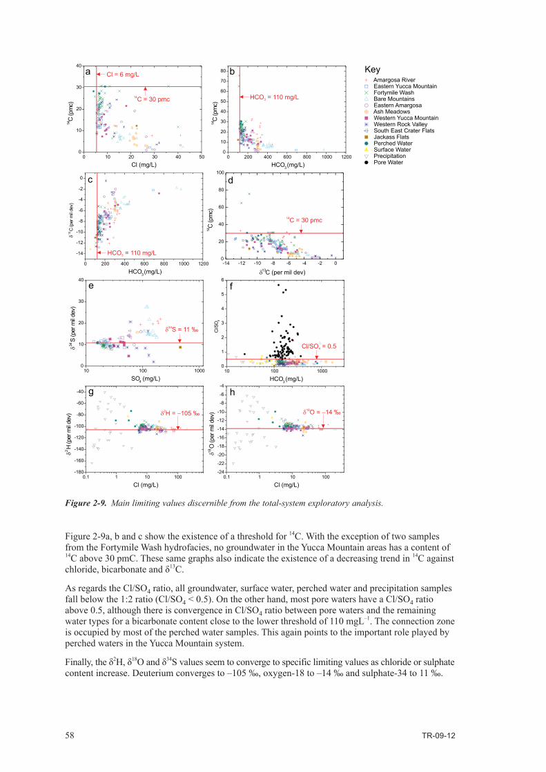
58 TR-09-12

Figure 2-9a, b and c show the existence of a threshold for 14C. With the exception of two samples from the Fortymile Wash hydrofacies, no groundwater in the Yucca Mountain areas has a content of 14C above 30 pmC. These same graphs also indicate the existence of a decreasing trend in 14C against chloride,bicarbonateandδ13C.

As regards the Cl/SO4 ratio, all groundwater, surface water, perched water and precipitation samples fall below the 1:2 ratio (Cl/SO4 < 0.5). On the other hand, most pore waters have a Cl/SO4 ratio above 0.5, although there is convergence in Cl/SO4 ratio between pore waters and the remaining water types for a bicarbonate content close to the lower threshold of 110 mgL–1. The connection zone is occupied by most of the perched water samples. This again points to the important role played by perched waters in the Yucca Mountain system.

Finally,theδ2H,δ18Oandδ34S values seem to converge to specific limiting values as chloride or sulphate contentincrease.Deuteriumconvergesto–105‰,oxygen-18to–14‰andsulphate-34to11‰.

Figure 2-9. Main limiting values discernible from the total-system exploratory analysis.

TR-09-12 59

Outliers The last observation that is worth noting from the total-system ion-ion plots is the existence of samples that are clearly way off the centre of gravity of the entire dataset. Figure 2-10 identifies the most obvious outliers (i.e. samples #2, #43, #44) together with some other potential ones (i.e. sample #256 or #160). The number of these samples is small but indicates the occurrence of extreme (and isolated) compositions that either do not follow specific trends or are separated by compositional gaps from the other samples. The total-system PCA that is presented below (see Figures 2-11 and 2-12) is also very useful for the identification of outliers and serves to improve this preliminary assessment. The samples identified as outliers will have a particular treatment when the hydrofacies exploratory analysis is carried out below.

Table 2-7 gives the maximum and minimum concentration values for all major and minor ions, stable isotopes and 14C. It gives the concentration and the sample number, together with the hydrofacies to which the sample belongs. Only groundwater samples (including perched waters) have been used to compile the table in order to clearly appreciate their heterogeneity. From the table it is clear that the upper concentration values for many chemical species (10 species) are found in water samples from the Ash Meadows hydrofacies (samples #2, 22, 43, 44, and 56). The ranking is followed by the perched water samples, which have maximum values in three chemical species (samples #336 and 345), then the Eastern Yucca Mountain (sample #206), Western Rock Valley (samples #196 and 201) and the Bare Mountain hydrofacies (#251, 254) with maximum values in two species, and finally the Amargosa River (#160), Western Yucca Mountain (#224) and Fortymile Wash (#359) hydrofacies with maximum values in one chemical species.

It is also interesting to note that two hydrofacies (Ash Meadows and Eastern Yucca Mountain) have samples with the minimum and maximum concentration values. This is the case for SiO2, where the minimum concentration is found in sample #44 (Ash Meadows) and the maximum concentration in sample #43 (Ash Meadows), and for iodine, with samples #314 (Eastern Yucca Mountain) having the minimum concentration value and sample #206 (Eastern Yucca Mountain) the maximum. This is an indication of extreme variability inside a hydrofacies, although it does not mean that all these samples are outliers. The hydrofacies exploratory analysis performed below will distinguish between outliers and extreme compositions.

Figure 2-10. Potential outlier samples identified in a Cl-Na ion-ion plot. Other potential outliers are also identified in Figure 2-12 below.

60 TR-09-12

Table 2-7. Maximum and minimum values for major and minor ions, stable isotopes and 14C. Only groundwater and perched water samples are included.

Species Minimum MaximumValue Sample # Value Sample #

Ca (mg/L) 0.28 340 147.7 336Mg (mg/L) 0.007 319 90 22Na (mg/L) 12.35 354 1,200 2K (mg/L) 0.95 336 83 2Cl (mg/L) 0.96 336 330 2HCO3 (mg/L) 70.4 345 1,690 43SO4 (mg/L) 4.3 336 1,100 2NO3 (mg/L) 0.02 25 , 305 , 326 62 160SiO2 (mg/L) 11 44 125 43F (mg/L) 0.22 345 15 44I (mg/L) 0.0005 314 0.16 206Br (mg/L) 0.02 291 , 345 15 206As (mg/L) 1.25 259 38 196B (mg/L) 80 21 12,000 44Sr (mg/L) 0.5 319 7,700 56Li (mg/L) 2 345 649 251U (mg/L) 0.2 4 , 259 10 224d2H (‰) –113.2 182 –73.1 345d18O (‰) –15.4 182 –9.9 345d13C (‰) –12.83 337 –0.5 201d34S (‰) 2.1 231 27.6 25414C (pmc) 0.94 167 75.7 359

Principal Component AnalysisPrincipal Component Analysis (PCA) is a powerful multivariate statistical technique for the analysis of large datasets using at the same time information from multiple compositional variables (Gómez et al. 2006). In this sense, it resembles a multidimensional version of the ion-ion plots presented in the previous section. The ability to simultaneously plot many compositional variables allows a better visual understanding of the system, pointing to the presence of trends, correlation and outliers that cannot be seen in any of the previous ion-ion plots in isolation.

Figure 2-11 plots the PCA performed on the raw dataset. The three first principal components have been plotted in three different graphs: pc1-pc2 (upper left-hand graph), pc1-pc3 (upper right-hand graph), and pc2-pc3 (lower graph). Each principal component is clearly related to a particular chemi-cal property of the water samples:

• Thefirstprincipalcomponent,pc1,isrelatedtothetotalcontentofdissolvedspecies,asindicatedby the original variables (shown as an axis eller axes in the figure). All the ionic variables point to the left-hand side of the plot, indicating that the content of all the chemical species increases to the left. Only the Na/Cl ratio, which is not a concentration, does not follow this rule.

• Thesecondprincipalcomponent,pc2,isrelatedtotheNa/Clratio,whichincreasesdownwardsinthe pc1-pc2 graph and to the left in the pc2-pc3 graph. Consequently, samples with a high Na/Cl ratio have a large and negative pc2 co-ordinate.

• Thethirdprincipalcomponent,pc3,isrelatedtothegeneralwaterchemistryofthesamples:Na-Cl waters (positive pc3 co-ordinate) versus Ca-Mg-HCO3 waters (negative pc3 co-ordinate).

TR-09-12 61

A PCA plot similar to the one in Figure 2-11 combines the information in a Piper diagram with that contained in several ion-ion plots viewed at the same time (amounting to all the possible combina-tions of two compositional variables). The usefulness and versatility of a PCA plot resides precisely in its ability to view the dataset from the most advantageous viewpoints, i.e. those that maximise the variance of the dataset in several mutually perpendicular axes. These axes are linear combinations of the original compositional variables and each one explains a decreasing amount of dataset variability. So, the first principal axis, pc1, “stores” the maximum amount of variance, followed by the second principal axis, pc2, which is perpendicular to the first one, and by the third principal axis, pc3, which is perpendicular to the other two. Each subsequent principal axis explains less and less variance, and is usually not taken into account.

Several trends are evident in the PCA plot of Figure 2-11. The most obvious ones are “the Na/ Cl trend”– with a vertical orientation in the pc1-pc2 graph – which includes most samples from the Western and Eastern Yucca Mountain hydrofacies, and the “carbonate trend”– best observed in the pc1-pc3 and pc2-pc3 graphs following the Ca and Mg vectors – which includes many of the samples from the South East Crater Flat, Bare Mountains and Ash Meadows hydrofacies, together with samples #306 (Eastern Yucca Mountain) and #307 (Western Yucca Mountain), taken at depth in the Palaeozoic Carbonate Aquifer under Yucca Mountain.

In addition to identifying trends, PCA plots are excellent tools for outlier screening, as the location of a sample in the plot is more extreme (in the sense of being far from the centre of gravity of the dataset, located at the origin of coordinates) the more extreme its global composition is (as opposed to extreme compositions in only one or two compositional variables). Figure 2-12 labels the most obvious outliers (numbered) identified in the PCA of the raw dataset. Again, as in the case of outlier

Figure 2-11. Three views of the Principal Component Analysis of the raw dataset. The upper left-hand graph plots the first and second principal components, the upper right-hand graph plots the first and the third principal components and the lower graph plots the second and the third principal components. Blue vectors are the original variable axes.

62 TR-09-12

screening by means of ion-ion plots, few samples belong to the category of outliers (remember that an outlier is defined here as a sample plotting far from the centre of gravity of the whole dataset); and if we compare the samples labelled in this figure with those labelled in Figure 2-10 and those presented in Table 2-7, we see many coincidences. All these samples will be analysed in the hydro-facies exploratory analysis.

2.4.2 Hydrofacies exploratory analysisThis section is dedicated to the exploratory analysis of each water category. The analysis starts with the ten groundwater categories and then continues with the other four water categories (perched waters, pore waters, surface waters and precipitation). The analysis of the groundwater hydrofacies starts with those at Yucca Mountain itself, followed by hydrofacies to the west and east of Yucca Mountain, and finally the hydrofacies south of Yucca Mountain (in the Amargosa River Valley).

Eastern Yucca Mountain ( )The samples of the Eastern Yucca Mountain hydrofacies have been collected from several boreholes in the eastern reaches of Yucca Mountain itself (Figure 2-13), in a north-south transect of approxi-mately 30 km.

The southern samples are from Nye County EWDP boreholes, and several of them actually perforate the Quaternary basin-fill deposits before reaching the Tertiary Tuffs Aquifer. The northern samples belong to several UE-25 and USW boreholes, and all of them perforate the Tertiary volcanic unsaturated formations before reaching the saturated zone, also in Tertiary volcanic rocks. Only borehole UE-25 p#1 reaches the Palaeozoic carbonate rocks located under the pile of Tertiary volcanic tuffs. Sample #307 was taken at the bottom of the borehole and is one of only two samples (sample #306 is the other) that can be used as being “representative” of the groundwaters in the Palaeozoic Carbonate Aquifer flowing under Yucca Mountain.

From the samples taken in NC-EWDP boreholes at several depths, cutting different aquifers, those from NC-EWDP 9D borehole are especially interesting because they show a mixing line between the Tertiary Tuff and Quaternary Alluvial waters. Figure 2-14 shows a summary lithology log of bore-hole 19D with the location of the packed-off sections where the samples were taken. Samples #204 to 207 are special as they were collected during a tracer test in which there was in-borehole mixing of waters from the two aquifers, i.e. the Quaternary Basin-fill Aquifer, where the samples were taken, and the Tertiary Tuffs Aquifer below. Consequently, sample #204 is the most “contaminated” with waters from the lower tuffs aquifer, while sample #207 is the least contaminated. The linear mixing trends resulting from this artificial mixing are evident from the graphs in Figure 2-14, especially in the one for HCO3-Na. The other packer-isolated samples collected in the same borehole also follow this mixing line, although no in-borehole contamination was reported in this case. An especially

Figure 2-12. Most obvious outlier samples identified in the PCA (labelled with sample ID).

TR-09-12 63

interesting aspect is that most of the other samples from the Eastern Yucca Mountain hydrofacies, coming from other boreholes, also follow the same mixing line (Figure 2-14), which suggests that both aquifers have a hydraulic connection.

The two mixed waters have a very similar chloride concentration, as the Cl-Na graph shows, with values of approximately 6 mg/L for both end-member waters. On the other hand, the concentrations of bicarbonate, calcium and sodium are very different. Also, from the HCO3-

14C plot, it appears that the Tertiary Tuff waters below Yucca Mountain have a 14C content of approximately 10 pmC, while that of the Quaternary basin-fill waters is higher (30 pmC).

In summary, sample #211 seems to be most representative of the composition of the Tertiary Tuff aquifer waters and is thus proposed for selection as a candidate end-member. Several samples can be proposed as candidates for the Quaternary basin-fill end-member (e.g. sample #207) although it is quite possible that some mixing with the Tertiary Tuff end-member is present even in the most extreme waters (those located in the lower left-hand corner of the HCO3-Na graph in Figure 2-14). Table 2-8 summarises the main chemical characteristics of both potential end-members.

Figure 2-13. Location map of the samples from the Eastern Yucca Mountain hydrofacies. Sample #307 from borehole UE25 p#1 was taken in the Palaeozoic Carbonate Aquifer that underlies the thick pile of Tertiary tuffs at Yucca Mountain. This sample has been omitted from the analysis carried out in this section (as the analysis is aimed at the behaviour of the Tertiary Tuffs Aquifer), but is not excluded from the final dataset and will be used in a subsequent section.

64 TR-09-12

Table 2-8. Chemical characteristics of two potential end-member waters.

Ion Tertiary tuffs end-member (#211) Quaternary basin-fill end-member

pH 8.9 8.0Cl (mg/L) 5.5 6–8 HCO3 (mg/L) 268.7 120–140SO4 (mg/L) 20.3 15–25Ca (mg/L) 0.57 16–18Na (mg/L) 113 40–5014C (pmC) 9.2 20–35

The general trend of the Ca-Na graph in Figure 2-14 is reminiscent of a cation-exchange process. This process has been identified in pore waters in the unsaturated zone at Yucca Mountain (Meijer 2002, Vaniman et al. 2001). However, cation-exchange is a thermodynamically fast process that occurs in zeolitised sections of the tuffs, already in the unsaturated zone. By the time these waters reach the saturated zone, they have acquired the cation-exchange signature of low divalent cation (Ca+Mg), high monovalent cation (Na+K) concentrations. For this reason, the main trends shown in Figure 2-14 are interpreted as mixing. The imprint of a Ca-Na exchange is the subset of samples that plot near the 1:2 molar ratio line and that clearly depart from the main mixing line in the Ca-Na graph in Figure 2-14. This additional trend suggests that some of the waters in the Tertiary Tuff Aquifer have passed through zeolitised tuffs before reaching the saturated zone whereas others have not. Few unsaturated-zone waters have been analysed for strontium isotopes, but the few that do have Sr isotopes data would appear to support this hypothesis (Sonnenthal and Bodvarsson 1999).

Figure 2-14. Mixing line between the Tertiary Tuffs and Quaternary Basin-fill Aquifers.

TR-09-12 65

Western Yucca Mountain ( )As the name suggests, the samples belonging to this hydrofacies are generally located on the west side of the crests that conform to the topmost part of Yucca Mountain. In addition to these samples, several others – located south of the main elevation – have been collected in NC-EWDP boreholes (Figure 2-15). Most samples were taken in Tertiary tuffs, although the boreholes in the southern part have Quaternary and Tertiary basin-fill deposits near the surface. Sample #306, collected at the bottom of borehole UE 25 p#1 in the Palaeozoic Carbonate Aquifer, has been omitted from the analysis.

Figure 2-16 plots the samples from the Eastern and Western Yucca Mountain hydrofacies together, using the same ion-ion and ion-isotopes plots as in Figure 2-14. As the geographic location and rock types are very similar in both hydrofacies, it is likely that their chemistry is also similar. In general terms, the plots confirm this hypothesis, although there are also obvious differences. In the bicarbonate-sodium plot, samples from this hydrofacies follow the mixing trend defined by the Eastern Yucca Mountain samples. As the occurrence of Quaternary basin-fill deposits in the Western Yucca Mountain hydrofacies is low compared with the Eastern part, most samples plot near the Tertiary tuffs end-member (two samples even further apart). Sample #327 seems to be an exception and a difficult one to interpret because this sample comes from the northernmost site, where no Quaternary basin-fill deposits exist. However, the Ca-Na graph shows that this sample plots on the Ca-Na exchange line, not on the mixing line.

Figure 2-15. Location map of the samples from the Western Yucca Mountain hydrofacies. Sample #306 from borehole UE25 p#1 was taken in the Palaeozoic Carbonate Aquifer that underlies the thick pile of Tertiary tuffs at Yucca Mountain. This sample has been omitted from the analysis carried out in this section.

66 TR-09-12

The Ca-Na plot shows that several Western Yucca Mountain samples are more depleted in Ca than their Eastern Yucca Mountain counterparts, suggesting a more widespread occurrence of cation-exchanged waters. This highly exchanged water comes from boreholes NC-EPDP 3S and 3D in the southernmost part of the area.

Chloride concentration is also somewhat higher than in the Eastern Yucca Mountain samples. However, with the exception of these differences, it can be safely concluded that both hydrofacies are affected by the same basic processes, i.e. mixing and cation-exchange, although the intensity of both is reversed.

Bare Mountain ( ) and South East Crater Flat ( )The samples of these two hydrofacies are similar both geographically and chemically. They are located in Crater Flat, a smooth surface limited in the west by the Bare Mountains and in the east by Yucca Mountain (Figure 2-17). Several samples have been collected close to the southern border of the area, near the Amargosa River Valley. Most samples come from packed sections in NC-EWDP boreholes, except for samples #293 (Bare Mountains hydrofacies) and #296 (South East Crater Flat hydrofacies), which were taken in open boreholes USW VH-1 and USW VH-2, respectively.

Chemically, the waters of both hydrofacies have a clear carbonate signature (see Figures 2-7 and 2-11 above). However, they have different TDS, with the South East Crater Flat samples being a diluted version of the Bare Mountains samples, as shown by Figure 2-18.

Four samples are clearly anomalous, as shown in the graphs in Figure 2-18. Sample #251 has very high Cl contents and sample #256 very high bicarbonate contents. Both also have a very poor charge balance, suggesting some kind of analytical error. On the other hand, samples #233 and 234 are anomalous in their Ca/HCO3 and Mg/HCO3 ratios, which is translated into a rather large degree of undersaturation with respect to calcite (and also dolomite). For these reasons, samples #233, 234, 251, and 256 have been omitted from further analysis.

Figure 2-16. Comparison of compositional trends in the Western and Eastern Yucca Mountain hydrofacies.

TR-09-12 67

Figure 2-17. Location map of the samples from the Bare Mountain (up triangle) and South East Crater Flat (barred left triangle) hydrofacies. Samples with anomalous Cl concentrations and calcite saturation indices have been highlighted.

Figure 2-18. Anomalous samples in the Bare Mountains (up triangles) and South East Crater Flat (barred left triangles) hydrofacies. All four anomalous samples have been eliminated from further analysis.

68 TR-09-12

Once these four samples have been eliminated, the remaining samples follow clear trends when SO4 is used as a proxy for evolution. Here, “evolution” could mean water-rock interaction, evaporation, mixing, or any other process that gradually changes the chemistry of the waters. Among all possible processes, dedolomitisation has been invoked elsewhere as the main process controlling the hydro-chemistry of carbonate aquifers in contact with gypsum (Plummer et al. 1990).

The trends followed by samples from the Bare Mountains and South East Crater Flat hydrofacies are reminiscent of a dedolomitisation process (Figure 2-19), except for the increase in bicarbonate with sulphate.

Dedolomitisation in a carbonate aquifer is a process driven by the presence of gypsum in the matrix or the fractures of the aquifer. At the start of the process, the waters are undersaturated with respect to gypsum. The dissolution of gypsum increases the concentration of Ca in the groundwaters which is then followed, promoted by the common ion effect, by the precipitation of calcite. As calcite precipitation takes place, pH and alkalinity decrease and the partial pressure of CO2 increases. This generates an undersaturation state for dolomite, which is thus dissolved, thereby increasing the concentration of Mg in the waters. In summary, as the concentration of sulphate increases, Ca, Mg and PCO2 also increase, and pH and alkalinity decrease. As Figure 2-19 shows, all the trends – except for alkalinity – are compatible with a dedolomitisation process.

To assess quantitatively the dedolomitisation hypothesis, several PHREEQC reaction-path simula-tions have been performed. Two different samples have been used as the initial water: #240 and #293 (both from the South East Crater Flat hydrofacies). The addition of gypsum is the irreversible process that drives dedolomitisation; a total of 1.5 mmol of gypsum in 100 steps have been added to span the

Figure 2-19. Evolution trends in the chemistry of the waters from the Bare Mountains (up triangles) and South East Crater Flat (barred left triangles) hydrofacies. Sulphate has been selected as a tracer of evolu-tion because dedolomitisation is a plausible process.

TR-09-12 69

measured sulphate concentration in groundwaters. In each reaction step, equilibrium with calcite and ordered dolomite has been imposed in a set of simulations, or with calcite and disordered dolomite in another set of simulations. The thermodynamic data have been taken from the WATEQ4F database distributed with the PHREEQC code.

Figure 2-20 shows, as a red line, the results from one of the dedolomitization simulations (sample #240 as initial water; equilibrium with calcite and ordered dolomite). The other simulations are not presented as the results are quantitatively very similar. It can be appreciated that no trend is quantitatively repro-duced, although qualitative tendencies are compatible with a dedolomitisation process in all cases apart from the alkalinity (bicarbonate) trend. Here the discrepancy is large because dedolomitisation implies a decrease in alkalinity with reaction progress. However, the observations made in the South East Crater Flat and Bare Mountain samples indicate the opposite trend: a large increase in alkalinity with sulphate. We conclude that dedolomitisation is not the process that is responsible for the chemistry of these waters.

However, dedolomitisation is not the only process that is capable of explaining the trend shown in Figure 2-19. Mixing between two suitable end-member waters is also a possibility. Another set of PHREEQC simulations has been performed with samples #264 and 293 as end-members. These are the most and least “evolved” waters in the combined Bare-Mountains + South East Crater Flat data-set. As Figure 2-19 shows, mixing between these two end-member waters could explain the trends observed, although with a certain scatter in several of the graphs. This points to the intervention of other processes on top of first order mixing. The chemical composition of the two end-member waters is presented in Table 2-9. Sample #264 can be considered as a potential end-member for the Palaeozoic Carbonate Aquifer waters. The more diluted SECF samples have a large contribution from a shallower component, either a shallow basin-fill groundwater or a “meteoric” water.

Figure 2-20. PHREEQC simulations of dedolomitisation (red line) and binary mixing (blue line) super-imposed onto the Bare Mountains (up triangles) and South East Crater Flat (barred left triangles) samples.

70 TR-09-12

Table 2-9. Chemical characteristics of the two end-member waters used in the mixing simulations carried out with PHREEQC.

Initial water (#293) (South East Crater Flat)

Final water (#264) (Bare Mountains)

pH 8.1 7.15Cl (mg/L) 8.8 22.5HCO3 (mg/L) 160.3 429.0SO4 (mg/L) 39.6 179.0Ca (mg/L) 11.4 82.5Mg (mg/L) 1.7 38.5Na (mg/L) 74.1 90.0d18O (‰) –14.3 –13.514C (pmC) 12.8 6.5

Jackass Flat ( )Jackass Flat is a smooth area east of Yucca Mountain, separated from it by Fortymile Wash. Its northern limit is the Calico Hills and its southern limit the Skull Mountains. Fortymile Wash connects Jackass Flat with the Amargosa River Valley to the South (Figure 2-21).

Only one sample (#291) is available from this region, collected in borehole UE25-J11. The water table was intersected at a depth of 317 m (REF) and the sampling interval includes the whole length of the borehole down to 405 m (open borehole sampling). The rocks of the saturated zone at the borehole site are tertiary basalts and tuffs. (CRWMS M&O 2007) made the assumption of considering this sample as being representative of the waters that flow under Jackass Flat. In this assessment, a different point of view is taken. Sample #291 is not considered a priori representative of the chemistry of the groundwaters in this part of the studied domain. An a posteriori decision will be taken based on the mixing analysis carried out with the M3 code below. Thus, sample #291 is selected as a potential end-member water and its main chemical characteristics are shown in Table 2-10.

Figure 2-21. Location map of the sample from the Jackass Flat. Only one sample is available from this geographical area and hydrofacies (sample #291, borehole UE25-J11).

TR-09-12 71

Table 2-10. Chemical characteristics of sample #291 (Jackass Flat hydrofacies).

Ion Jackass Flat (sample #291)

pH 7.9Cl (mg/L) 22.4 HCO3 (mg/L) 100.6SO4 (mg/L) 467.2Ca (mg/L) 80.8Mg (mg/L) 14.4Na (mg/L) 154.514C (pmC) 12.3

Western Rock Valley ( )Samples from the Western Rock Valley hydrofacies are located near the south-eastern end of Yucca Mountain, between Fortymile Wash and the Specter Range (Figure 2-22). All samples except one have been taken in the flat area delimitated by Fortymile Wash and the foothills of the Specter Range. The only exception is sample #182, which was collected in a hilly area of the Specter Range.

This dataset consists of 18 samples with Cl contents of between 5 and 32 mgL–1 following quite simple increasing trends with Na, HCO3, Mg, etc. The only clear departure from this trend is sample #182, which has high HCO3 and Mg values (actually this sample is oversaturated in dolomite and in equilibrium with magnesite, whereas all the other samples in the dataset are undersaturated in dolomite and magnesite). For all these reasons, sample #182 has been excluded from the dataset.

The Cl-14C plot again suggests a mixture with a low-Cl, high-14C end-member. When this mixing proportion is low (low 14C values), the Cl content of the waters is in the range of 30 mgL–1. This is a further indication that the Quaternary Alluvial waters, when not “contaminated” by the precipitation end-member, have a Cl concentration of the order of 30 mgL–1. Although low in comparison with groundwaters elsewhere, this amount of chloride (30 mgL–1) seems to be the highest in the whole Yucca Mountain dataset when evaporation is excluded.

Figure 2-22. Location map of the samples from the Western Rock Valley. Two samples with an anomalous chloride concentration are highlighted (samples #200 and 201). Sample #182 has been excluded from the final dataset, as discussed in the text.

72 TR-09-12

Fortymile Wash ( )The 55 samples assigned to the Fortymile Wash hydrofacies come from a broad region that encompasses a sizable part of the Fortymile Wash river, from its northern reaches in the Calico Hills down to the Amargosa River Valley (Figure 2-24). The southern samples are flanked to the west by the Amargosa River hydrofacies and to the east by the Eastern Amargosa hydrofacies. The samples have been collected in packed-off NC-EWDP boreholes and in other open-hole boreholes, including water wells and irrigation wells, all of them in Quaternary basin-fill deposits.

In general, the chemistry of this hydrofacies is rather diluted, with average Cl contents of 6 to 12 mgL–1, although four samples (#125, 133, 138, and 156) have higher chloride concentrations of up to 61 mgL–1 (sample #125). Actually, the samples from the Fortymile Wash hydrofacies have the lowest TDS of all the groundwaters in the dataset.

The four samples with higher Cl contents (highlighted in Figure 2-24) seem to have an evaporation signature (all of them are located in the centre of the Amargosa Valley). Also, two of these high-Cl samples (#125 and #133) have raised concentrations of NO3, possibly due to contamination with fertilizers (these two samples come from the Amargosa Farms region, an area where artificial irriga-tion is widespread). Consequently, the four samples with Cl > 15 mgL–1 have been excluded from the final dataset.

As regards 14C contents, all samples except two (#359 and 360) have 14C < 32 pmC. This 14C value was identified in the total-system exploratory analysis as a threshold for the complete dataset, not only for the Fortymile Wash hydrofacies. The two samples enriched in 14C, clearly contaminated by recent meteoric water, come from the northern part of the region (Figure 2-24), where precipitation is higher.

Figure 2-23. Main trends in the Western Rock Valley hydrofacies.

TR-09-12 73

The last graph in Figure 2-25 is a Principal Component Analysis including only samples from the Fortymile Wash hydrofacies. The graph shows the pc1-pc2 plane and here it is obvious that most samples occupy a compact region near the origin of coordinates. Several samples lie further apart, including the four samples with high contents of Cl.

Apart from outliers, the identification of trends in a dataset is important in order to interpret its origin and evolution. As Figure 2-26 shows, trends are not very clear. It is worth noting that the variability in Cl contents is much smaller than in other ions or isotopes. This gives vertical “trends” for many ions and isotopes when plotted against chloride. It should be noted that the two samples with a high 14C value systematically lie in the lower concentration range of these vertical “trends”. In other words, these samples are more diluted that most samples, although their Cl content is similar to the others. One possible interpretation is mixing between two waters with the same concentration of chloride (approximately 10 mgL–1) but different concentration of the other ions and isotopes. From the graphs in Figures 2-25 and 2-26, the range of concentration values summarised in Table 2-11 can be deduced for the Quaternary (Fortymile Wash) basin-fill end-member water.

Figure 2-24. Location map of the samples from the Fortymile Wash hydrofacies. Samples with anomalously high chloride contents are highlighted. The southern end of the area has been enlarged (image lower left).

74 TR-09-12

Figure 2-25. Outliers in Fortymile Wash hydrofacies. Samples with Cl > 15 mg/L and 14C > 32 pmc are considered anomalous. (a) Frequency histogram of chloride concentrations; (b) Cl-SO4 ion-ion plot; (c) Cl-14C plot; (d) pc1-pc2 view of a PCA using only the Fortymile Wash samples.

Figure 2-26. Ion-ion and ion-isotopes plots for the Fortymile Wash hydrofacies. Samples #359 and 360, with an anomalously high value of 14C, are labelled.

TR-09-12 75

If the values shown in the second columns of Table 2-11 are compared with those shown in the last column of Table 2-8 for the potential Quaternary basin-fill end-member as deduced from Eastern Yucca Mountain samples (appended here as Column 3), their similarity is obvious. Although the pH value is slightly lower in the potential end-member deduced from the Fortymile Wash samples (7.5–7.9 versus 8), and the Ca content slightly higher (20 mgL–1 versus 16–18 mgL–1), it had already been noted that the potential end-member deduced from the Eastern Yucca Mountain hydrofacies was quite possibly contaminated to some extent by waters from the Tertiary Tuffs Aquifer. As a conse-quence, the pH and concentration values shown in Table 2-11 could be a better approximation to the “pure” Quaternary basin-fill end-member water.

Amargosa River ( )Samples from the Amargosa River hydrofacies occupy the central and north-western parts of the Amargosa Valley (Figure 2-27). Most of them come from an area where irrigation is widespread and have been collected from shallow water wells. A group of samples have been collected near the southern end of the Bare Mountains (samples #276–287), some 30 km northwest of the remaining samples.

Three groups of water samples can be distinguish with respect to chloride: a low-Cl group, with chloride contents of between 30 and 40 mgL–1; a medium-Cl group, with chloride contents ranging from 60–85 mgL–1; and a high-Cl group (sample #160), with Cl = 123 mgL–1. In general, chloride concentrations are high compared with the other elements in this hydrofacies (the mean Cl content is 24.5 mgL–1 and the median value is 11.4 mgL–1 for the whole raw dataset, see Figure 2-3 and Table 2-5).

This hydrofacies is difficult to interpret. Cl trends are not easily attributed to evaporation, as most ions do not increase their concentration with chloride, with the exception of SO4. In particular, Ca and Mg are more or less independent of the concentration of Cl, although Mg (not Ca) does tend to increase with bicarbonate (Figure 2-28). Calcite and dolomite are in equilibrium or slightly over saturated in these samples, suggesting precipitation of calcite and/or dolomite. Samples #97 (Cl = 78 mg/L) and #160, from the Amargosa Farms region, have high concentrations of NO3, which suggests the possibility of contamination by fertilizers.14C trends are also intriguing (Figure 2-28), as the percentage of modern carbon seems to increase with Cl and decrease with HCO3. This is unexpected from both the evaporation and mixing points of view.

The lowest Cl contents are approximately 30 mgL–1, much higher than in the Quaternary Alluvial end-member deduced from the Eastern Yucca Mountain and Fortymile Wash datasets.

A more reliable interpretation of this hydrofacies has been deferred to the Results section, when several hydrofacies from the Quaternary Basin-fill Aquifer in the Amargosa River Valley (Amargosa River, Eastern Amargosa, Western Rock Valley and Fortymile Wash hydrofacies) will be plotted together.

Table 2-11. Chemical characteristics of a potential end-member water for the Quaternary Basin-fill Aquifer (second column), compared with the composition suggested for the same end-member after analysis of the Eastern Yucca Mountain samples (appended here as Column 3).

Ion Quaternary basin-fill end-member (Fortymile Wash)

Quaternary basin-fill end-member (from Table 2-8)

pH 7.5–7.9 8.0Cl (mg/L) 6–8 6–8 HCO3 (mg/L) 120–160 120–140SO4 (mg/L) 20–30 15–25Ca (mg/L) 20 16–18Na (mg/L) 40 40–5014C (pmC) 18–30 20–35

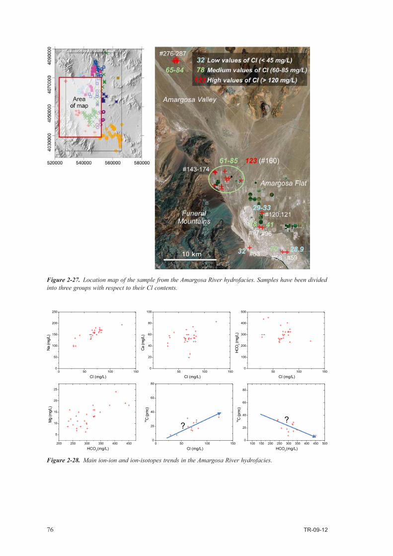
76 TR-09-12

Figure 2-27. Location map of the sample from the Amargosa River hydrofacies. Samples have been divided into three groups with respect to their Cl contents.

Figure 2-28. Main ion-ion and ion-isotopes trends in the Amargosa River hydrofacies.

TR-09-12 77

Eastern Amargosa ( )The samples belonging to the Eastern Amargosa hydrofacies occupy a compact area in the central part of the Amargosa River Valley, between the Fortymile Wash samples to the east and the Ash Meadows samples to the southwest (Figure 2-29). All samples were taken from shallow water wells, either for domestic use or for irrigation. The water table in the area is at a depth of 5 to 50 metres below ground level, saturating Quaternary basin-fill deposits.

Hydrochemically, the composition of the samples is fairly homogeneous. The normal chloride content in the waters of this hydrofacies ranges from 16 to 31 mgL–1, although three samples have anomalously low Cl (9–10 mgL–1) and one sample has an anomalously high Cl of 41 mgL–1 (these samples are highlighted in Figure 2-29).

Figure 2-30 shows several ion-ion, ion-isotope and isotope-isotope plots which together suggest that the waters from the Eastern Amargosa hydrofacies can be described as a rather simple mixture of two end-member waters: a low-Cl, high-14C,heavy-δ18O end-member and a high-Cl, low-14C, light-δ18O end-member. A representative composition of both end-members is displayed in Table 2-12

The low-Cl end-member water has a chemical composition compatible with the potential Quaternary Basin-fill Aquifer end-member suggested by the analysis carried out with Eastern Yucca Mountain and Fortymile Wash hydrofacies, although the concentration of Na is higher here (100–120 mgL–1 versus 40–50 mgL–1). The high-Cl end-member, however, has not been identified in the analysis of the previous hydrofacies. Only some samples from the Amargosa River hydrofacies (those lowest in chloride) have a chemical signature similar to the high-Cl end-member identified here. The significance and origin of this end-member will be discussed below in a combined analysis of all the hydrofacies connected with the Quaternary Basin-fill Aquifer (i.e. the Amargosa River, Eastern Amargosa, Fortymile Wash and Western Rock Valley hydrofacies).

Sample #127 has the highest Cl concentration and departs from most trends as shown in Figure 2-30. Forthisreason,ithasbeenexcludedfromthefinaldataset.Sample#104isanomalousintheδ18O-14C plot, but since it behaves “normally” in the other plots it has been retained in the final dataset.

Figure 2-29. Location map of the sample from the Eastern Amargosa hydrofacies. Samples low and high in chloride have been highlighted. The normal chloride contents in this hydrofacies are between 16 and 31 mgL–1.

78 TR-09-12

Table 2-12. Chemical characteristics of two potential end-member waters from the Eastern Amargosa hydrofacies.

High-Cl end-member (Eastern Amargosa)

Low-Cl end-member (Eastern Amargosa)

pH 7.5–7.7 8.0–8.1Cl (mg/L) 25–32 7–10HCO3 (mg/L) 270–320 100–125SO4 (mg/L) 140–170 20–30Ca (mg/L) 45–55 15–20Mg (mg/L) 12–21 2–4Na (mg/L) 100–120 18–25K (mg/L) 10–18 7–10d18O (‰) –13.8 –13 to –12.814C (pmC) 0–5 25–35

Figure 2-30. Chloride trends (visual aid only) for the Eastern Amargosa hydrofacies. These trends are compatible with a binary mixture of two end-member waters. The high-Cl, low-14C end-member is marked with a blue circle. Sample #127 is anomalous as it departs from most trends. Also, its chloride content is the highest.

TR-09-12 79

Central Amargosa Valley combined analysisAfter dealing in the last four sections with the four hydrofacies geographically located around the central section of the Amargosa River Valley (Amargosa River, Eastern Amargosa, Fortymile Wash, and Western Rock Valley), a combined analysis is performed here with the aim of characterising, from a broader viewpoint, the common trends and the heterogeneity. For this purpose, several ion-ion plots and a PCA will be used. All the samples from these hydrofacies were sampled in the Quaternary Basin-fill Aquifer.

Figure 2-31 shows several ion-ion and ion-isotopes plots for the combined dataset. It is immediately obvious that the four hydrofacies share a common evolution, with the Fortymile Wash hydrofacies being those that are less “evolved” (i.e. more diluted), and the Amargosa River hydrofacies those that are most “evolved” (i.e. less diluted). Samples from the Eastern Amargosa hydrofacies systematically plot in a middle position, while samples from the Western Rock Valley hydrofacies tend to plot close to the Fortymile Wash ones, although the scatter is greater.

The end-member water already identified in the previous sections is here even more patent. It has been marked with a red ellipse in several of the plots in Figure 2-31. Inside the ellipse, samples from the Fortymile Wash, Eastern Amargosa and Western Rock Valley are found, which means that this “pure” end-member water has a widespread occurrence in the alluvial deposits.

The “evolved” end of the trends behaves differently. This part of the trend is only occupied by the Amargosa River hydrofacies when chloride or sulphate are used as markers of evolution or shared with some of the Eastern Amargosa hydrofacies when bicarbonate is used for that purpose (but bicarbonate is not a conservative element in this system). Sample #160 seems to be an outlier, although it follows the common trends in most graphs. Sample #143 has also been highlighted in Figure 2-31 as the most evolved sample in the cluster that can be observed in the Cl plots. The composition of this sample is summarised in Table 2-13 and it will be added to the potential end-member list.

Figure 2-31. Main trends for all the hydrofacies of the central part of the Amargosa Valley.

80 TR-09-12

Ash Meadows ( )The Ash Meadows region is located in the south-eastern corner of the domain studied (Figure 2-32). The region belongs to the Amargosa River Valley and is the exit point for the superficial waters in the domain, which flow south and then west towards Death Valley. Groundwaters in this area flow through Quaternary basin-fill deposits of varied lithology, ranging from coarse siliciclastic to tuffaceous to evaporitic. The dataset consists of 49 samples taken from shallow wells (27 samples) and springs (22 samples). Most of the springs are located in a spring line which is the surface expression of the Gravity Fault.

As was already evident in the total-system exploratory analysis, this hydrofacies contains several of the most extreme samples, which points to the operation of an array of processes that modify in a rather strong way the original chemistry of the groundwaters. Because many samples have been collected in springs and shallow irrigation boreholes, evaporation is an issue here and must be taken into account. Also, the presence of scattered playa deposits with highly soluble evaporitic minerals should be borne in mind when trying to interpret the hydrochemistry of several samples.

Table 2-13. Chemical characteristics of sample #143 (Amargosa River hydrofacies) as potential end-member water for the high-Cl Quaternary Basin-fill Aquifer waters.

High-Cl end-member (Amargosa River)

pH 7.69Cl (mg/L) 83 HCO3 (mg/L) 235SO4 (mg/L) 235Ca (mg/L) 66Mg (mg/L) 11Na (mg/L) 170K (mg/L) 12d18O (‰) Not analyzed14C (pmC) Not analyzed

Figure 2-32. Location map of the sample from the Ash Meadows hydrofacies. Samples low and high in chloride have been highlighted.

TR-09-12 81

Chloride ranges from 6.8 to 330 mgL–1, sulphate from 37 to 1,100 mgL–1, bicarbonate from 157 to 1,690 mgL–1, Na from 52 to 1,200 mgL–1, Ca from 1.3 to 140 mgL–1, Mg from 1 to 90 mgL–1 and K from 6.2 to 69 mgL–1. All of these upper values are the highest in all the groundwater hydrofacies (see Table 2-7).

Figure 2-33 plots the main trends in the Ash Meadows hydrofacies. Outliers already discovered in the total-system analysis are also detected here. As none of the high-TDS samples were analysed for isotopes (2H,δ18O,δ34S,δ13C and 14C), trends of chloride against the isotopes are incomplete, spanning only the 0–30 mgL–1 Cl range (Figure 2-34). This is problematic as several of these trends could distinguish between evaporation and other processes responsible for raised concentrations of chloride (e.g. dissolution of evaporitic minerals).

Figure 2-33. Main trends in the Ash Meadows samples. High-TDS samples are labelled. The blue line in several plots marks the molar ratio of the two ions. The 1:1 line in the Cl-Na plot represents halite dissolu-tion, the 1:2 line in the SO4-Na plot represents thenardite dissolution and the 2:3 line in the HCO3-Na plot represents trona dissolution.

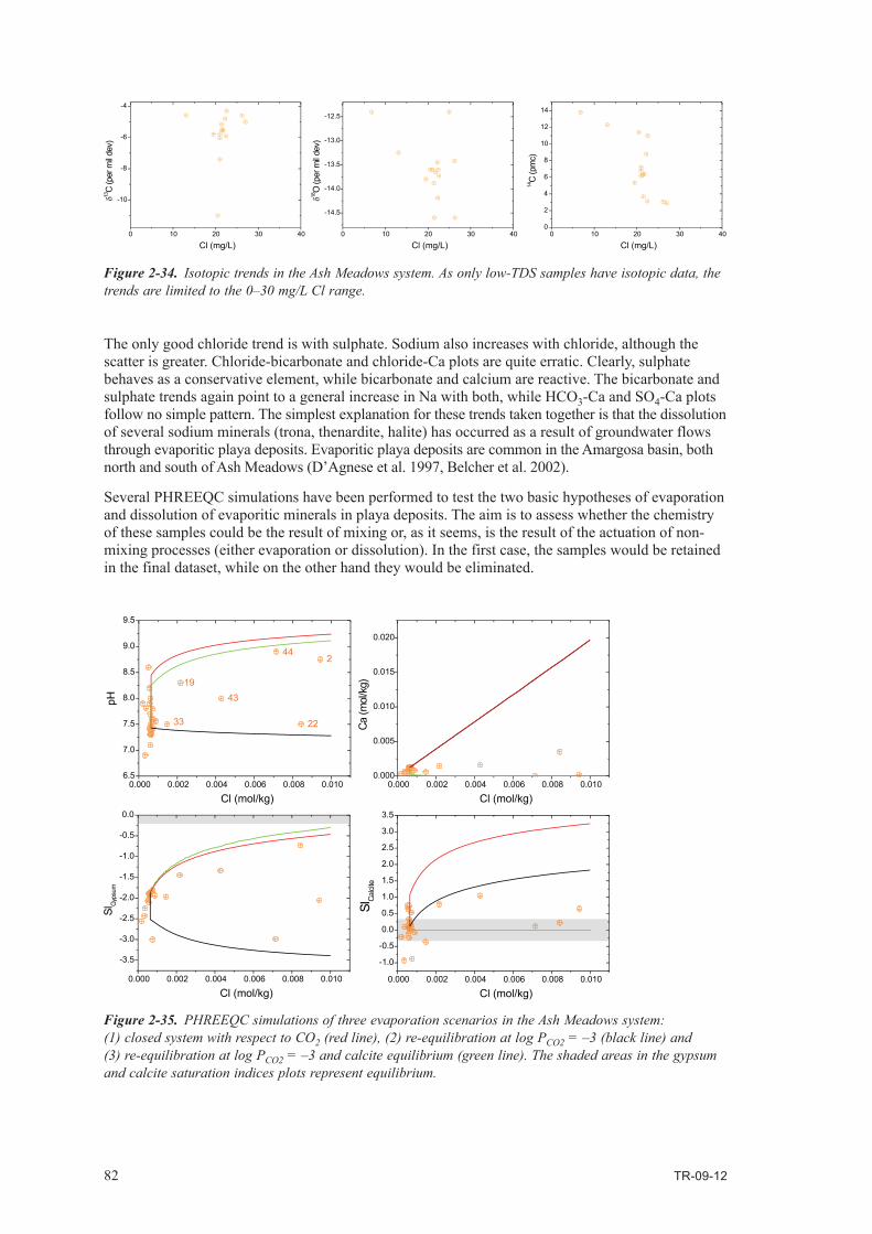
82 TR-09-12

The only good chloride trend is with sulphate. Sodium also increases with chloride, although the scatter is greater. Chloride-bicarbonate and chloride-Ca plots are quite erratic. Clearly, sulphate behaves as a conservative element, while bicarbonate and calcium are reactive. The bicarbonate and sulphate trends again point to a general increase in Na with both, while HCO3-Ca and SO4-Ca plots follow no simple pattern. The simplest explanation for these trends taken together is that the dissolution of several sodium minerals (trona, thenardite, halite) has occurred as a result of groundwater flows through evaporitic playa deposits. Evaporitic playa deposits are common in the Amargosa basin, both north and south of Ash Meadows (D’Agnese et al. 1997, Belcher et al. 2002).

Several PHREEQC simulations have been performed to test the two basic hypotheses of evaporation and dissolution of evaporitic minerals in playa deposits. The aim is to assess whether the chemistry of these samples could be the result of mixing or, as it seems, is the result of the actuation of non-mixing processes (either evaporation or dissolution). In the first case, the samples would be retained in the final dataset, while on the other hand they would be eliminated.

Figure 2-34. Isotopic trends in the Ash Meadows system. As only low-TDS samples have isotopic data, the trends are limited to the 0–30 mg/L Cl range.

Figure 2-35. PHREEQC simulations of three evaporation scenarios in the Ash Meadows system: (1) closed system with respect to CO2 (red line), (2) re-equilibration at log PCO2 = –3 (black line) and (3) re-equilibration at log PCO2 = –3 and calcite equilibrium (green line). The shaded areas in the gypsum and calcite saturation indices plots represent equilibrium.

TR-09-12 83

Three different constraints have been imposed in the evaporation simulations: (1) closed system with respect to CO2, (2) re-equilibriation at PCO2 = 10–3 (normal CO2 partial pressure in the unsaturated zone at Yucca Mountain) and (3) re-equilibration at PCO2 = 10–3 and equilibrium with calcite. These three types of simulations span the main potential scenarios during evaporation in the Ash Meadows area.

Figure 2-35 presents the results using chloride as the variable that defines the degree of evaporation. The red line represents the evolution in the closed-system scenario, the black line the evolution in the re-equilibrium at PCO2 = 10–3 scenario and the green line the evolution in the scenario where both re-equilibrium at PCO2 = 10–3 and equilibrium with calcite are imposed. None of the scenarios match the evolution of the whole dataset, although the third scenario, in which precipitation of calcite is allowed, correlates better with the low concentration of Ca in most high-TDS samples. In light of these results, it is concluded that evaporation does not seem to be the key process responsible for the anomalous chemistry of some of the Ash Meadows waters, although it may have affected them.

In addition to evaporation simulations, several mass-balance calculations using the inverse-problem methodology implemented in the PHREEQC code were also performed. Sample #40 was used as the initial water (diluted initial state), while samples #2 and #44 were the final waters (concentrated final state). Several evaporitic minerals were included in the calculations: calcite, gypsum, halite, trona (Na3H(CO3)2:2H2O), natron (Na2CO3:10H2O) and several borates. This set of minerals has been selected as they are cited as feasible phases in playa deposits from the Amargosa River and Death Valley regions (Claassen 1985). Borates have also been included as samples #2 and #44 are highly enriched in boron (8.9 ppm in sample # and 12 ppm in sample #44), and large borate deposits are known in the region.

PHREEQC gives 36 different models, which vary in the number of phases included and the amount of dissolution (mass transfer) for each mineral. However, most of them give precipitation of calcite and the dissolution of gypsum, halite, trona and several borates. These mass transfers are capable of explaining the compositional change between the initial and the final waters, including, most importantly, the change in alkalinity, sodium, and boron, and the reduced pH of the final waters (approximately 8.9). Consequently, it can be concluded that the dissolution of evaporitic minerals would appear to be the cause of the anomalous compositions of most high-TDS samples in the Ash Meadows area, although evaporation could also have played a minor role. For all these reasons, the following samples have been eliminated from the dataset (in decreasing chloride concentration): 2, 22, 44, 43, 51, 29, 19, 84, 33 and 32. Sample #56 is also eliminated because it is anomalous with respect to bicarbonate.

Apart from the obvious heterogeneity of compositions in the Ash Meadow hydrofacies as a whole, there is a group of samples (24 in all, i.e. 50% of all the hydrofacies samples) with a narrow range of values for many of the major ions. The average composition of these waters is summarised in Table 2-14. In addition to the chemical parameters in Table 2-9, the representative waters of the Ash Meadows hydrofacies have a rather high CO2 partial pressure (logPCO2 = –2.0).

Table 2-14. Chemical characteristics of the representative samples from the Ash Meadows hydrofacies.

Representative samples (Ash Meadows)

pH 7.3–7.5Cl (mg/L) 20–24 HCO3 (mg/L) 280–320SO4 (mg/L) 80–100Ca (mg/L) 42–52Mg (mg/L) 20–23Na (mg/L) 70–100d18O (‰) 13.9 to –13.214C (pmC) 4–12

84 TR-09-12

Geographically, most of these samples are located on or near the surface expression of the Gravity Fault, which is a discharge area for groundwaters that seem to have flowed through the Palaeozoic Carbonate Aquifer (their temperature is systematically higher than that of other samples in the Ash Meadows area). Samples with higher or lower concentrations are located west and south of the Gravity Fault, although three high-Cl samples are also on the fault line (Figure 2-32), indicating either evaporation or dissolution of evaporitic minerals.

The set of 20 samples with a narrow range of concentrations will be considered as being representa-tive of the unaltered hydrochemistry of the Ash Meadows waters. “Unaltered” means not modified by evaporation and/or dissolution of evaporitic minerals, although mixing with other types of water could be the reason for their (rather small) range of compositions. This set of samples, together with the samples eliminated from the dataset, are displayed in Table 2-15

Perched waters ( ), pore waters ( ), surface waters ( ), and precipitation ( )Apart from the groundwater samples, the raw dataset contains four other water categories: pore waters, perched waters, surface waters and precipitation. The location and sample number of all these non-groundwater samples is shown in Figure 2-36. This dataset contains 6 perched water samples, 81 pore water samples, 17 surface water samples and 39 precipitation samples. Some or all of these water categories should represent the “initial state” from which the chemistry of the already described groundwaters evolves (by evaporation, water-rock interaction, mixing, etc).

Table 2-15. Ash Meadows samples separated into three groups: representative samples, excluded samples and non-representative but non-excluded samples.

Representative samples (24) Excluded samples (8) Non-representative, non-excluded samples (18)

3, 17, 18, 20, 21, 23, 26, 27, 28, 31, 35, 36, 40, 41, 47, 48, 52, 81, 82, 85, 86, 90, 92, 99

2, 19, 22, 29, 32, 33, 43, 44, 51, 56, 84

4, 5, 24, 25, 34, 36, 37, 38, 39, 46, 49, 54, 93, 94, 103

Figure 2-36. Location and sample number of the four non-groundwater water categories in the raw dataset.

TR-09-12 85

In this sense it is important to assess the similarities and differences between these water categories in order to identify the most probable initial state. This “initial state water” would be one of the basic end-members from which the chemistry of the groundwater samples should be built. The basic pre-requisite for a water to be the initial state for groundwater evolution is that a smooth and continuous chemical transition exists between the initial water and the most dilute groundwaters.

With this objective in mind, Figure 2-37 plots the most interesting ionic trends in the non-ground-water dataset. Chloride is used as the marker of evolution in the first three plots, bicarbonate in the fourth and calcium in the other two. The Cl-SO4 plot, as already commented on in the total-system exploratory analysis, shows a very good correlation between the concentrations of both ions. The red line gives the 1:1 Cl to SO4 molar ratio. All samples follow this line apart from certain pore waters, which are depleted in sulphate (for a given value of chloride).

In the Cl-HCO3, Cl-Na, HCO3-SO4 and Ca-Na graphs in Figure 2-37 two trends are clearly distinguish-able: one followed by the precipitation and surface water samples, and another followed by the pore water samples. In all cases, the perched water samples plot in the intersection of both trends (blue circle). As will be seen later, this is also the convergence point for the most diluted groundwaters in the dataset (Fortymile Wash hydrofacies).

Another crucial observation to be made from Figure 2-37 is the existence of a compositional gap between precipitation and surface waters on the one hand and the pore waters on the other, which is better appreciated in the Cl-Na and Ca-Na plots. Perched water samples fill this gap, giving continuity to the geochemical evolution of the waters. In other words, the perched waters seem to be playing the role of a “hinge” between the evolution trends of surface waters (including precipitation) and pore waters. It should be noted, however, that certain surface waters (and even some of the most concentrated precipitation samples) plot also in this compositional gap (see, for example, the Cl-SO4 plot in Figure 2-37).

Figure 2-37. Main ionic trends in the non-groundwater samples. The perched water sample #336, with an anomalous chemistry, is labelled.

86 TR-09-12

All the above observations point to the important role that perched waters play in the Yucca Mountain system. Precipitation and surface waters are, of course, more “pristine” than perched waters, but they are not justifiable as the initial water from which the evolution of the groundwaters starts. This function seems to be neatly fulfilled by the perched waters.

Nevertheless, precipitation and surface waters will also be used as potential end-members in the next section. For this purpose, two candidate samples will be selected here by means of a Principal Components Analysis to serve as end-members. Figure 2-38 shows the result of the PCA in the pc1-pc2 plane. The original compositional variables are also included to establish that all the variables point to the left of the graph. This means that samples to the left of the pc1 = 0 coordinate have a higher TDS than the others. In other words, more diluted samples (less evolved ones) are on the right and less diluted samples (more evolved) are on the left. A compact cluster of precipitation samples is evident in the right-hand part of the graph. These are precipitation samples with a low TDS that share a similar chemical signature. Thus, a sample near the centre of this cluster could be a good candidate for the precipitation end-member. Sample #6221, labelled in Figure 2-38 has been selected.

With regard to the surface water samples, it is also clear from the PCA plot that there is a trend towards increasing TDS. This could be related to evaporation and/or dissolution of minerals during surface flow. Consequently, a good candidate for a potential surface water end-member would be the less evolved sample (minimum TDS). For this reason, sample #275 has been selected.

For the M3 analysis that is carried out in the next section, only the two samples from the surface water and precipitation dataset will be used.

The pore water samples have a wide compositional range. Some samples are diluted and similar in chemistry to the perched waters and the most diluted groundwaters (e.g. those of the Fortymile Wash hydrofacies). However, other samples, which are located far from the convergence zone between the surface waters and precipitation trend on the one hand and the pore waters trend on the other, are clearly affected by additional processes (evaporation, ion-exchange, dissolution and/or precipitation of minerals, Meijer 2002). Furthermore, the PCA carried out in the total-system exploratory analysis (see Figure 2-11 above) demonstrates that these samples follow specific trends, different from those followed by the groundwaters. Owing to the clear chemical discrepancies, it has been decided that the pore water samples should be excluded from the final dataset.

Figure 2-38. Principal component analysis of the precipitation and surface waters. The two samples selected as potential end-members are labelled.

TR-09-12 87

2.4.3 Conclusions of the exploratory analysis

• Followingthehydrofaciesexploratoryanalysis,threemaingroupsofgroundwaterhydrofaciesare apparent: (1) hydrofacies related to the Regional Palaeozoic Carbonate Aquifer (Bare Mountains, South East Crater Flat, Ash Meadows and samples #306 and 307), (2) hydrofacies clearly related to the Tertiary Tuffs Aquifer (Eastern and Western Yucca Mountain) and (3) hydrofacies related to the Quaternary Basin-fill Aquifer (Amargosa River, Eastern Amargosa, Fortymile Wash and Western Rock Valley). This last group of waters seems to be the most heterogeneous and difficult to interpret.

• Tothesethreegroupsofgroundwater,theperchedwatersshouldbeaddedasthe“initial”waterfrom which all the others evolve. Modern precipitation and surface waters are not taken into account as they do not seem to be directly related to the general dynamics of the Yucca Mountain hydro-system. However, one sample of the precipitation samples and another from the surface water samples will be included in the following M3 analysis as potential end-member waters.

• Apreliminaryidentificationofend-memberwatersforeachgroupofhydrofacieshasbeencarriedout and their chemical characteristics summarised in tables.

• Fromthetotal-systemandhydrofaciesexploratoryanalysis,severalsampleshavebeenidentifiedas being the results of the actuation of a varied array of processes which have drastically modified their chemical composition. These samples, collected in Table 2-16, have been excluded from the final dataset. None of the analyses carried out in the next section include these samples. In summary, the final dataset has 240 samples.

Table 2-16. Excluded samples after the total-system and hydrofacies exploratory analyses.

Hydrofacies Water type Symbol Excluded samples

Amargosa River Ground waterEastern Yucca Mountain Ground waterFortymile Wash Ground water #125, #133, #138, #156Bare Mountain Ground water #233, #234, #251, #256Eastern Amargosa Ground water #127Ash Meadows Ground water #2, #19, #22, #29, #33, #43, #44, #51Western Yucca Mountain Ground waterWestern Rock Valley Ground water #182South East Crater Flats Ground waterJackass Flat Ground waterPerched Water Perched water #336Surface Water Surface water All except sample #275Precipitation Precipitation All except sample #6221Pore Water Pore water All

TR-09-12 89

3 M3 analysis: selection of end-member waters and calculation of mixing proportions

M3 is a Principal Component Analysis code that approaches the modelling of mixing and mass bal-ance from a purely geometrical perspective (Laaksoharju et al. 1999, Gómez et al. 2006, 2009). Unlike standard geochemical codes, M3 tries first to explain the chemical composition of a parcel of water by pure mixing, and only then are deviations from the pure mixing model interpreted as chemical reactions.

The M3 multivariate approach uses several chemical and physicochemical variables (conservative and non-conservative) to construct an ideal linear mixing model of the groundwater system. This is done by performing a Principal Component rotation of an n·n covariance matrix, where n is the number of chemical and physicochemical variables (e.g. Gershenfeld 1999). Each element of the covariance matrix expresses the degree of correlation of a pair of variables. Graphically, this is equivalent to the rotation of a reference frame composed of n orthogonal axes (one axis for every variable) until one axis, the first principal component, points in the direction of the maximum variability of the data set; another axis, the second principal component, points in the perpendicular direction with the second-largest variability and so on for the other axes. Once the samples and the end-members have been expressed in the Principal Component co-ordinates, mixing proportions are calculated in a straightforward way as the local co-ordinates of each sample in a hyper-tetrahedron whose vertices are the end-members (Gómez et al. 2006). This hyper-tetrahedron is a simplex, and therefore always has as many dimensions as end-members minus one.

Because there is one co-ordinate (i.e. one axis) for each input variable, at least as many input variables as end-members minus one are needed to obtain the mixing proportions (e.g. if three input variables are being used, say the concentration of Cl, Br and 18O, it would be possible to give mixing proportions between two, three or a maximum of four end-member waters).

M3 calculates the mixing proportions with an algorithm referred to as ‘‘n-principal component mixing” (Gómez et al. 2006). This algorithm uses all principal components to compute the mixing proportions (geometrically, it works in an n-dimensional space, where n is the number of input compositional variables).

Once the mixing proportions have been calculated, the constituents that cannot be described by mixing are described using reactions by simple elemental mass balance supported by independent knowledge of the system. Reactions are inferred heuristically (by inspection) from the difference, for each sample, between the actual value of an input variable and the value computed by M3 assuming pure mixing. For example, if there is a deficit of both Ca and HCO3 in the computed composition compared with the actual Ca and HCO3 contents, it could be inferred that calcite has precipitated. There is no rigorous statistical test to decide whether a deviation between the computed and the analysed concentration of an element in a sample is sufficient to invoke a reaction.

3.1 Selection of end-member watersThroughout the previous section, a number of water compositions have been collected in tables. Some have already been identified as potential end-members, others were used as initial or final waters in PHREEQC simulations and others were simply catalogued as being “representative” of a particular hydrofacies (e.g. the Ash Meadows hydrofacies). Table 3-1 compiles all these samples with their main chemical characteristics. In those cases where a range of concentrations has been specified for a potential end-member, a specific sample from the dataset is chosen, complete with the concentration of all the key chemical elements within the proposed range (i.e. representative of the given compositional range).

90 TR-09-12

Table 3-1. Potential end-member waters used in the M3 analysis.

Sample Hydrofacies Ca Mg Na K Cl HCO3 SO4 Cl/Na

143 AR ( ) 66.00 11.000 170.00 12.00 83.00 235.00 235.00 2.05207 EYM ( ) 16.00 1.700 49.50 3.85 6.30 144.00 21.00 7.86211 EYM ( ) 0.57 0.027 113.00 3.51 5.50 268.74 20.30 20.5359 FmW ( ) 16.00 2.390 35.60 4.31 8.34 112.00 16.50 4.27264 BM ( ) 82.50 38.250 90.00 6.10 22.50 429.00 179.00 4.0088 EA ( ) 19.43 1.950 40.67 7.51 9.01 125.95 29.70 4.51164 EA ( ) 51.00 18.000 103.00 13.00 30.00 288.00 143.00 3.4340 AM ( ) 46.25 20.550 74.10 9.03 22.20 316.00 80.80 3.34293 SECF ( ) 11.42 1.680 74.10 2.11 8.83 160.25 39.60 8.39291 JaF ( ) 80.81 14.410 154.48 16.00 22.42 100.61 467.19 6.89345 PW ( ) 7.05 0.916 16.30 6.38 3.03 70.42 4.88 5.37275 SW ( ) 6.70 0.70 2.40 6.30 2.00 31.72 6.30 1.206221 P ( ) 0.64 0.04 0.68 0.23 0.59 0.82 3.66 1.15

If the end-members have been correctly chosen for the given dataset, all samples should plot inside an n –1-dimensional hyper-volume defined by the n end-members (Gómez et al. 2006). This is a generalisation of the property of triangular coordinates, i.e. any point inside the triangle has all three triangular coordinates positive, and any point outside the triangle has at least one negative coordinate. By applying this rule, it is easy to know which samples fall inside the hyper-volume defined by the n end-members: those with all their mixing proportions positive. Only these samples can be “explained” by pure conservative mixing of the selected end-members. The closer the number of explained samples is to the total number of samples, the better the combination is (in the sense that more samples can be explained as a mixing of the selected end-members). In other words, a set of end-members is properly selected for a specific dataset when most of the waters in the dataset fall inside the mixing hyper-volume. For three end-members, the mixing hyper-volume is simply a triangle; for four end-members, a tetrahedron and for five or more end-members, a hyper-tetrahedron (Gómez et al. 2006).

M3 performs a systematic search of combinations, starting from two end-members and ending with the maximum number of end-members included as input potential end-members (Gómez et al. 2006). The total number of combinations grows rapidly with this maximum number. For 13 potential end-members, those compiled in Table 3-1, the total number of combinations is 8,178. In other words, M3 solves the mixing problem for all the samples in the dataset a total of 8,178 times, each time selecting a different combination of potential end-members and computing the percentage of samples (coverage) that can be explained by mixing the chosen end-members. The “best” combinations of end-member waters are those with a higher coverage; in other words, with a higher percentage of samples inside the mixing polyhedron. Table 3-2 shows all the combinations of end-member waters with a coverage of at least 75%. This means that at least three quarters of the samples in the final dataset are inside the hyper-tetrahedron defined by the end-members that are listed in the first column of the table. The calculations were made using the same 8 compositional variables already used in the total-system exploratory analysis, i.e. Ca, Mg, Na, K, Cl, HCO3, SO4 and the Cl/Na ratio.

The “best” combination has a coverage of 92.4% and is defined by end-members #143, 211, 264 and 6221. Sample #143 is the high-Cl sample from the Amargosa River hydrofacies, sample #211 is the “Tertiary Tuffs aquifer” end-member selected from the Eastern Yucca Mountain hydrofacies, sample #264 is the final water (more evolved) in the PHREEQC mixing and dedolomitisation calculations from the Bare Mountain and South East Crater Flat hydrofacies (the water with the clearest signature of the Palaeozoic Carbonate aquifer) and sample #6221 is the precipitation sample that was chosen as representative of all the precipitation samples in the raw dataset.

TR-09-12 91

The second “best” combination, with a coverage of 88.6%, shares with the best combination three of the four end-members. However, the precipitation sample #6221 has been substituted here by surface water sample #275. The third “best” combination again has the same end-members as the first, except for sample #143, which in this combination has been substituted by sample #291 (the lone sample from the Jackass hydrofacies).

The analysis of Table 3-2 shows that only a subset of all the potential end-member waters partici-pates in “good” combinations. For example, all of the 14 combinations shown in the table include sample #211 (the Tertiary Tuffs Aquifer end-member), and 9 combinations (out of 14) include sample #264 (the Palaeozoic Carbonate Aquifer end-member).

But even more interesting than the specific end-members which are included in good combinations is the observation that only combinations with three and four end-member waters appear in Table 3-2. Considering that M3 has systematically computed all the possible combinations, starting with two end-members and ending with 13 end-members, this is a clear indication that the Yucca Mountain hydro-system must be the result of mixing between a maximum of four different water types. The best combination of 5 end-members, [143 211 264 345 6221], only explains 42.2% of the samples, and the best 6 end-member combination, [40 143 211 291 345 6221], just 36.6% of the samples. Both combinations are far from the 92.4% coverage that the best 4 end-member combination provides.

Figure 3-1 shows on pc1-pc2 plots the coverage of the end-member combinations listed in Table 3-2. It is clear from the figure that 3 end-member combinations are worse that 4 end-member combinations (even 3 end-member combinations with a higher coverage than 4 end-member combinations) as they leave an important part of the volume occupied by the samples outside the mixing hyper-tetrahedron. This is evident, for example, when comparing the best 3 end-member combination (rank 4 in Table 3-2, located in the second row, first column in Figure 3-1; coverage: 85.1%), with 4 end-member combina-tion rank 6 (second row, third column in Figure 3-1; coverage: 84.3%). Although the coverage is slightly higher in the 3 end-member combination, a large group of samples located in the upper right-hand corner of the pc1-pc2 plot are not explained by mixing. On the other hand, in the 4 end-member combination most of these samples are inside the mixing hyper-tetrahedron1. Thus, coverage is only a fast way of ranking the mixing models, but the actual principal component analysis results must

1 Notice that the area inside the triangle defined by the three end-members in 3 end-member combinations is the actual mixing “hyper-volume”, but that the area inside the four-sided polygon defined by the four end-members in 4 end-member combinations is only the projection on to the pc1-pc2 plane of a three-dimensional tetrahedron. This is why some of the samples that appear to be inside this projected tetrahedron are actually outside it in the real three-dimensional mixing space.

Table 3-2. Combinations of end-member waters with a coverage > 75%. Selected mixing models are highlighted in blue.

Rank End-member combination Coverage Mixing model

1 [143 211 264 6221] 92.4 MM1

2 [143 211 264 275] 88.6

3 [211 264 291 6221] 88.1 MM2

4 [211 264 275] 85.1

5 [211 264 275 291] 84.3

6 [211 264 6221] 85.1

7 [211 264 345] 82.6

8 [143 211 264 345] 81.4 MM3

9 [40 143 211 6221] 80.9 MM4

10 [211 264 291 345] 79.7 MM5

11 [40 211 291 6221] 79.2 MM6

12 [211 275 291] 77.9

13 [40 143 211 275] 75.8

14 [143 211 275] 75.3

92 TR-09-12

also be taken into account. Based on both the coverage and the actual distribution of the excluded samples, it is concluded that 3 end-member combinations are not able to correctly model the mixing behaviour of waters at Yucca Mountain. Therefore, only 4 end-member combinations are further analysed. In other words, 4 end-member mixing models explain the hydrochemistry of the Yucca Mountain area better than 3 end-member mixing models.

The first three entries in Table 3-2 are 4 end-member combinations. The end-members that are included in these three combinations are only 7 (of the potential 13 end-member listed in Table 3-1): one is always the sample that was considered as being representative of the Tertiary Tuffs Aquifer (TTA) (sample #211), another is always the sample considered as being representative of the Regional Palaeozoic Carbonate Aquifer (RCA) (sample #264), another is always a “meteoric water” sample

Figure 3-1. M3 screenshots showing the 14 combinations of end-members with a coverage > 75%, ordered by decreasing coverage from the upper left to the lower right. Results of the principal components analysis are projected on to the pc1-pc2 plane (pc1 runs horizontally and pc2 vertically). The end-members that define each combination are labelled. Samples inside the mixing polyhedron are coloured in blue while those outside it are coloured in black.

TR-09-12 93

(either surface water #275 or precipitation water #6221) while the fourth is always a sample repre-sentative of the Quaternary Basin-fill Aquifer (QBfA) (the high-Cl samples #143 from the Amargosa River hydrofacies, or sample #291 from the Jackass Flat hydrofacies).

It is interesting to note that the next best 4 end-member combination (rank eight in Table 3-2) has as “meteoric” end-member, the perched water sample #345. This confirms the comment in the hydro facies exploratory analysis section on the important role that perched waters play in the Yucca Mountain system.

So, it is observed that either a precipitation sample, a surface water sample or a perched water sample always appears as an end-member water in all the good 4 end-member combinations. To combine all three possibilities under one name for this end-member, the term “altered meteoric water” (AMW) end-member will be used from now on. The name can be a little misleading when the “pure” precipitation sample #6221 is used as the actual AMW end-member, but it is preferable to the plain “meteoric end-member”, as it emphasizes that water-rock interaction processes have already modified the chemistry of this end-member water. Precipitation sample #6221 is the less modified “altered meteoric” end-member, and perched water sample #345 is the most evolved “altered meteoric” end-member, while surface water sample #275 lies somewhere in between. Thus, mixing proportions obtained with mixing models that include sample #275 would lie within the range defined by mixing models that use sample #6221 or #345. As the range of mixing propor-tions is most interesting, all 4 end-member combinations in which sample #6221 or #345 defines the altered meteoric end-member will be tested, and all combinations in which sample #275 is the altered meteoric end-member will be omitted.

Figure 3-2 shows three perpendicular views of the PCA performed on the final dataset. The end-members giving good coverage are labelled in the figure. It can be observed that they actually occupy extreme positions in the Principal Components graphs.

Figure 3-2. Three perpendicular views of the PCA carried out with the final dataset. The end-member waters identified with M3’s End-member Selection Module and belonging to mixing models with a coverage > 75% are labelled. Also, special samples 306 and 307 are labelled and encircled.

94 TR-09-12

It should also be noted that the two samples collected in the Palaeozoic Carbonate Aquifer in borehole UE-25 p#1 (samples #306 and 307) are outside the mixing polyhedron. This means that the chemical composition of samples #306 and 307 cannot be explained by a pure mixture of the four end-member waters (samples #143, 211, 264, and 6221). Other M3 runs were performed using the other combinations of end-members listed in Table 3-2, and in each case samples #306 and 307 were outside the mixing polyhedron. Two possible explanations for this difference in chemistry are: (1) the groundwaters of the carbonate aquifer under Yucca Mountain do not mix with other ground-waters included in the final dataset nor discharge inside the studied domain and (2) other processes besides mixing have change their chemistry, “pushing” both samples outside the mixing polyhedron.

3.2 Test of mixing modelsThe analysis carried out in the preceding section has shown that 4 end-member mixing models are superior to 3 end-member models. All the 4 end-member mixing models with > 75% coverage (Table 3-2) have several properties in common, which are important to stress in this context:

• Fromthe13potentialend-memberwaterslistedinTable3-1only8appearin“good”combina-tions (those with > 75% coverage, as listed in Table 3-2). These are samples #40 (AM), #143 (AR), #211 (EYM), #264 (BM), #275 (SW), #291 (JaF), #345 (PW) and #6621 (P).

• Every4end-membercombinationinTable3-2hasanAlteredMeteoricend-member(sample#6621, sample #345 or sample #275), a Palaeozoic Carbonate Aquifer end-member (either sample #264 or sample #40), a Tertiary Tuffs Aquifer end-member (sample #211) and a Quaternary Basin-fill Aquifer end-member (either sample #143 or sample #291).

• AlteredMeteoricend-memberwatersareofthreetypes:precipitation(#6621),surfacewater(#275) and perched water (#345). Surface waters have a chemical signature intermediate between precipitation and perched waters (see, for example, Figures 2-37 and 3-2), which is the reason why mixing models that have sample #275as Altered Meteoric end-member surface water are not taken into account. Also, surface water samples could have been subjected to water-rock interaction processes that are not representative of those that characterise the recharge waters which eventually enter the groundwater system. Thus, only mixing models in which the Altered Meteoric end-mem-ber is occupied by precipitation sample #6621 or perched water sample #354 have been selected. These mixing models, highlighted in Table 3-2, are compiled in Table 3-3 indicating which sample occupies the Altered Meteoric Water (AMW), the Regional Palaeozoic Carbonate Aquifer (RCA), the Tertiary Tuffs Aquifer (TTA) and the Quaternary Basin-fill Aquifer (QBfA) end-member. Also, a specific label (MM1 for mixing model #1, MM2 for mixing model #2, and so on) is given to each of them for further reference (in order of decreasing coverage).

However, coverage is not the only attribute of a “good” mixing model (as already observed when comparing three- and four-end-member mixing models). Obviously, a key aspect for classifying a mixing model as being good or bad is how well the chemical composition of conservative elements (such as chloride) can be reproduced. This is easily performed once the mixing proportions have been computed. An example using Cl as the conservative element will clarify the procedure.

Table 3-3. Selected mixing models indicating the sample acting as end-member (sample number and hydrofacies) and the coverage.

Mixing model End-member combination CoverageAMW RCA TTA QBfA

MM1 6221 264 211 143 92.4MM2 6221 264 211 291 88.1MM3 345 264 211 143 81.4MM4 6221 40 211 143 80.9MM5 345 264 211 291 79.7MM6 6221 40 211 291 79.2

: Precipitation; : Perched water; : Bare Mountain; : Ash Meadows; : Eastern Yucca Mountain; : Amargosa River; : Jackass Flat.

TR-09-12 95

Assuming that the mixing proportions of sample #3 (from the Ash Meadows hydrofacies) calculated with mixing model #1 (MM1) are: AMW = 22.1%, RCA = 48.3%, TTA = 9.0% and QBfA = 20.6%, the chloride contents of the four end-member waters are (Table 3-1): AMW (#6621) = 0.59 mgL–1; RCA (#264) = 22.5 mgL–1; TTA (#211) = 5.5 mgL–1) and QBfA (#143) = 83.0 mgL–1. Thus, the predicted chloride concentration of sample #3 under mixing model #1 is:

AM PCA TTA QBfASample #3

Cl 22.1% Cl 48.3% Cl 9.0% Cl 20.6%Cl 28.6 mg/L

100= = .

· · · ·+ + +

As the actual chloride concentration of sample #3 is Cl = 25.0 mgL–1, mixing model #1 overestimates the Cl content by 3.6 mgL–1 in absolute terms (12%). Therefore, when plotting the calculated Cl concentration of each sample against its actual concentration on an XY graph, a good model should have most samples along the 1:1 diagonal line.

Figure 3-3 plots the measured and calculated chloride concentrations in the six mixing models, with the measured concentration in the horizontal axis and the calculated one in the vertical axis. Each mixing model is represented by two plots: the left-hand plot is drawn with linear scales and the right-hand one with log-log scales to better appreciate the low-concentration end. Visually, it seems clear that models MM2 and MM5 are the worst of the group, whereas models MM1, MM3 and MM4 perform much better. Model MM6 appears to lie somewhere in between.

Obviously, a more quantitative assessment of the quality of each mixing model is needed. The whole procedure can be boiled down into a goodness-of-fit exercise, where the “model” is the diagonal line in Figure 3-3 and the “observations” are the samples. The closer to the diagonal line the samples are, the better the fit and the smaller the mismatch between measured and computed concentrations (residuals). Two goodness-of-fit statistics have been used to compare the six mixing models: the coefficient of determination (R2), which is appropriate for absolute deviations, and the chi-square statistics, χ2, which is useful for assessing relative deviations.

The coefficient of determination is defined as:

2 err

tot

SS1

SSR = − ,

where SStot is the total sum of squares and SSerr is the sum of squared errors (or residual sum of squares),

ob ob 2tot

1

SS ( )N

i ii

x m=

= −∑ ,

ob cal 2err

1

SS ( )N

i ii

x x=

= −∑ .

In the expression for SStot,μreferstothemeanvalueofvariablex. For linear regression, as here, the coefficient of determination is the square of the well-known correlation coefficient and is a statistical measure of how well the regression line approximates the real data points. An R2 of 1.0 indicates that the regression line fits the data perfectly, while an R2 of 0.0 indicates that none of the variance in the data is explained by the proposed model. An intermediate value (such as R2 = 0.7) means that part of the variance in the data is captured by the model (in the example, 70%), but another part (here 30%) is not explained and can be assigned to unknown variables or inherent variability. When comparing different models, the best model is the one with an R2 value closest to 1. Table 3-4 gives the coefficient of determination for the six mixing models. We can see that the “intuitive” ranking of the models based on Figure 3-3 is qualitatively correct. Models MM1, MM3 and MM4 all have R2 values of between 0.82 and 0.87, whereas models MM2 and MM5 have R2 values of approximately 0.32, and model MM6 is intermediate, with R2 = 0.47.

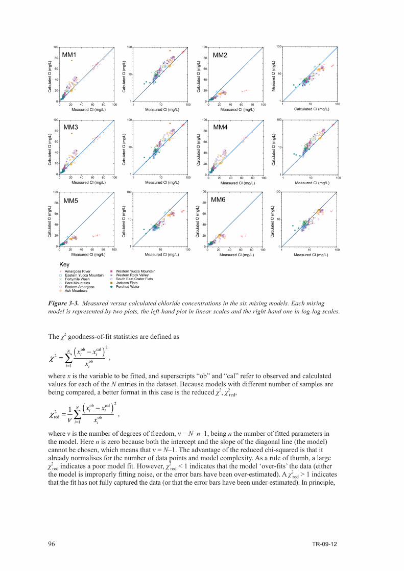
96 TR-09-12

The χ2 goodness-of-fit statistics are defined as

( ) 2ob cal

2ob

1

Ni i

i i

x x

xc

=

−= ∑ ,

where x is the variable to be fitted, and superscripts “ob” and “cal” refer to observed and calculated values for each of the N entries in the dataset. Because models with different number of samples are being compared, a better format in this case is the reduced χ2, χ2

red,

( ) 2ob cal

2red ob

1

1 Ni i

i i

x x

xc

ν =

−= ∑ ,

whereνisthenumberofdegreesoffreedom,ν=N–n–1, being n the number of fitted parameters in the model. Here n is zero because both the intercept and the slope of the diagonal line (the model) cannotbechosen,whichmeansthatν=N–1. The advantage of the reduced chi-squared is that it already normalises for the number of data points and model complexity. As a rule of thumb, a large χ2

red indicates a poor model fit. However, χ2red < 1 indicates that the model ‘over-fits’ the data (either

the model is improperly fitting noise, or the error bars have been over-estimated). A χ2red > 1 indicates

that the fit has not fully captured the data (or that the error bars have been under-estimated). In principle,

Figure 3-3. Measured versus calculated chloride concentrations in the six mixing models. Each mixing model is represented by two plots, the left-hand plot in linear scales and the right-hand one in log-log scales.

TR-09-12 97

a χ2red = 1 is the best fit for the given data and error bars. When comparing different models, the best

model is the one with a χ2red closest to 1 (from above). Table 3-4 gives the reduced χ2 for the six mixing

models. Contrary to the coefficient of determination results, in this case model MM6 is the “best” one, followed by models MM3 and MM4, while model MM5, as was the case with R2, is the “worst” one.

Table 3-4. Chloride goodness-of-fit for the six mixing models highlighted in Table 3-2.

Mixing model N SStot SSerr R2 Rank c2 Rank

MM1 222 57,738.9 10,635.1 0.816 3 2.80 5MM2 210 37,934.0 25,545.8 0.327 5 2.71 4MM3 196 56,312.9 7,939.1 0.859 2 2.10 2MM4 194 47,546.7 5,995.0 0.874 1 2.12 3MM5 189 36,705.3 25,061.8 0.317 6 2.86 6MM6 187 27,364.4 14,524.4 0.469 4 1.66 1

As the coefficient of determination is, in this case, a measure of the goodness-of-fit of a linear regression model by least squares (minimisation of the sum of squared errors), outliers can drastically affect the quality of the fit. This is clearly the case with model MM6: it has a low R2 of 0.47 (rank 4) but is the model with the lowest reduced χ2 (rank 1). Going back to Figure 3-3 it can be appreciated that a group of outlier samples in the high-Cl end (samples from the Amargosa River hydrofacies) is obviously increasing the sum of squared errors (and thus reducing the overall coefficient of determi-nation). On the other hand, models MM3 and MM4 do not have these outliers (see again Figure 3-3) and the overall R2 is much higher (0.86 and 0.87, respectively).

However, it is important to note that the six mixing models have a different number of samples (“observations”). Although this is somehow taken into account by both the R2 approach (via the total sum of squares) and the χ2

redapproach(viathenumberofdegreesoffreedom,ν),theexclusionofdifferent samples in each case can, if these samples are far from the average deviation, influence the outcome of the statistical test. To take this asymmetry into account, both R2 and χ2

red for the subset of samples common to the six mixing models (this subset is composed of 164 samples) have been recomputed. Table 3-5 gives the new results. Now, on a common basis of the same 164 samples, MM3 emerges as the “best” model in both the R2 and χ2

red senses while MM6 ranks second from the χ2

red point of view and fourth from the R2 point of view.

Combining the rankings from coverage, R2 and χ2 (Table 3-6), mixing model MM3 emerges as the “best” model overall, followed (closely) by MM1 and by MM4 in the third position. So, MM3 will be taken as the reference mixing model in the next section and the mixing proportions obtained from it will be compared with the other mixing models in order to assess the variability of the results. Summating ranks of different statistics (coverage, R2, χ2) does not seem very appropriate, more so when the statistics have been obtained in rather different ways. And it would really be inappropriate if each set of statistics gave a completely different ranking. However, this is not the case, as model MM3 is the best model in both the R2 and χ2 senses. This is the only factor necessary in order to give model MM3 the status of “reference model”. Below, reference model MM3 will be compared to the other models, and in making these comparisons the actual ranking of the other models (as summarised in Table 3-6) becomes quite irrelevant.

98 TR-09-12

Table 3-5. Chloride goodness-of-fit (reduced to a common set of samples) for the six mixing models highlighted in Table 3-2.

Mixing model N SStot SSerr R2 Rank c2 Rank

MM1 164 26,013.3 4,891.1 0.812 3 2.09 3MM2 164 26,013.3 16,524.9 0.365 5 2.36 5MM3 164 26,013.3 3,646.0 0.860 1 1.36 1MM4 164 26,013.3 4,782.7 0.816 2 2.10 4MM5 164 26,013.3 16,700.2 0.358 6 2.41 6MM6 164 26,013.3 14,203.5 0.454 4 1.80 2

Table 3-6. Final ranking of the six mixing models taking into account coverage, R2 and c2 rankings ( : Precipitation; : perched water; : Bare Mountain; : Ash Meadows; : Eastern Yucca Mountain; : Amargosa River; : Jackass Flat).

Mixing model End-member combination Rank Cov

Rank R2

Rank c2

Sranks Final rankAMW RCA TTA QBfA

MM3 345 264 211 143 3 1 1 5 1MM1 6221 264 211 143 1 3 3 7 2MM4 6221 40 211 143 4 2 4 10 3MM2 6221 264 211 291 2 5 5 12 4MM6 6221 40 211 291 6 4 2 12 51)

MM5 345 264 211 291 5 6 6 17 61) Although mixing models MM2 and MM6 have the same sum of ranks, MM6 is given a lower final rank due to its smaller coverage.

TR-09-12 99

3.3 Mixing proportionsMixing model MM3 gives the best overall performance for the description of the Yucca Mountain hydro-system in terms of mixing. Here “best” is used qualitatively, meaning better global performance. However, as we have seen above, mixing model MM3 is also the best model in both the quantitative R2 sense as well as in the quantitative χ2 sense. For this reason, model MM3 is regarded as the reference mixing model and the mixing proportions obtained with it are considered as being the “good ones”. Table 3-7 gives the mixing proportions of all samples in the final dataset for reference mixing model MM3. Samples outside the mixing polyhedron are included in the table but have no mixing proportions. Samples are ordered in increasing sample number (abbreviated to ID# in the table heading) and the symbol identifying the hydrofacies (see above) has been added to facilitate the visual analysis of the table.

Table 3-7. Mixing proportions of samples in the final dataset for mixing model MM3.

ID# TTA RCA QBfA AMW ID# TTA RCA QBfA AMW

3 0.065 0.466 0.195 0.274 197 0.167 0.077 0.011 0.7454 0.073 0.400 0.256 0.271 198 0.057 0.090 0.040 0.8135 0.055 0.444 0.220 0.281 199 0.404 0.028 0.092 0.47717 0 0.530 0.087 0.384 200 0.233 0.017 0.505 0.24518 0 0.536 0.053 0.411 201 0.156 0 0.376 0.46820 0 0.518 0.076 0.406 202 0.831 0 0.041 0.12821 0 0.516 0.066 0.419 203 0.738 0.005 0.026 0.23123 – – – – 204 0.829 0 0.026 0.14524 0.141 0.108 0.087 0.664 205 0.542 0 0.035 0.42325 0.049 0.660 0.067 0.225 206 0.477 0 0.047 0.47626 0 0.506 0.118 0.376 207 0.230 0.054 0.018 0.69827 – – – – 208 0.347 0.014 0.031 0.60828 0 0.527 0.062 0.411 209 0.729 0 0.043 0.22831 0 0.529 0.059 0.412 210 0.919 0 0.005 0.07734 0 0.157 0.387 0.456 211 1.000 0 0 035 – – – – 212 0.154 0.045 0.041 0.75936 0.267 0.341 0.220 0.172 213 0.707 0 0.040 0.25337 0.133 0.204 0.154 0.509 214 0.868 0 0 0.13238 0.056 0.206 0.346 0.392 215 0.824 0.017 0 0.16039 0.398 0.144 0.179 0.279 216 0.747 0 0.035 0.218

40 0 0.533 0.091 0.375 217 0.552 0.012 0.019 0.417

41 0 0.505 0.105 0.390 218 0.755 0 0.009 0.236

45 0 0.277 0.334 0.390 219 0.634 0 0.047 0.318

46 0.311 0.290 0.210 0.189 220 0.568 0.044 0 0.389

47 0 0.519 0.075 0.407 221 0.272 0.038 0.039 0.651

48 0 0.541 0.063 0.397 224 0.831 0 0.143 0.026

49 0.158 0.105 0.069 0.668 225 – – – –

52 0 0.540 0.055 0.405 226 0.643 0 0.128 0.229

58 0 0.134 0.820 0.046 227 0.265 0.028 0.034 0.673

59 0.028 0.312 0.327 0.334 228 0.295 0.112 0.062 0.530

63 0.025 0.600 0.370 0.005 230 – – – –

81 0 0.511 0.073 0.416 231 – – – –

82 0 0.500 0.083 0.418 232 0.143 0.080 0.293 0.484

85 0 0.510 0.068 0.421 235 0 0.691 0.025 0.283

86 – – – – 236 0.262 0.169 0.082 0.488

88 0 0.065 0.099 0.836 237 0.281 0.164 0.064 0.490

89 – – – – 238 0.275 0.153 0.071 0.502

100 TR-09-12


90 – – – – 239 0.256 0.154 0.082 0.508

92 0 0.534 0.060 0.406 240 0.188 0.116 0.142 0.553

93 0.100 0.408 0.241 0.251 241 0.129 0.118 0.007 0.74694 0.107 0.259 0.315 0.319 242 0.055 0.126 0.019 0.80095 0.024 0.093 0.055 0.829 243 0.084 0.094 0.020 0.80296 – – – – 244 0.086 0.069 0.028 0.81697 – – – – 245 0.158 0.123 0.013 0.70699 0 0.519 0.075 0.406 246 0.084 0.149 0.008 0.759101 0 0.237 0.415 0.348 247 0.049 0.095 0.028 0.828102 0.042 0.097 0.099 0.762 248 0.112 0.059 0.039 0.791103 0.108 0.169 0.458 0.265 249 0.286 0.047 0.028 0.639104 0 0.091 0.167 0.742 250 0.642 0 0.086 0.272105 – – – – 252 0 0.764 0 0.236106 – – – – 253 0 0.758 0 0.242107 – – – – 254 0 0.774 0 0.226116 0.083 0.075 0.054 0.788 255 0 0.782 0.009 0.209117 0.059 0.089 0.044 0.808 258 – – – –120 0.033 0.265 0.280 0.422 259 0.087 0.519 0.089 0.305121 0 0.317 0.366 0.318 260 – – – –122 0 0.091 0.083 0.826 261 – – – –123 – – – – 262 – – – –124 0 0.316 0.445 0.239 263 0 0.959 0 0.041126 0 0.422 0.358 0.220 264 0 1.000 0 0128 0.080 0.069 0.050 0.801 265 0.183 0.038 0.054 0.725129 0 0.376 0.406 0.218 266 0.099 0.064 0.044 0.793130 0 0.467 0.391 0.142 267 0.115 0.062 0.039 0.784131 0.237 0.053 0.163 0.546 268 0.114 0.054 0.050 0.782136 0.018 0.051 0.107 0.825 269 0.118 0.057 0.036 0.789137 0.038 0.092 0.062 0.808 270 0.580 0 0.120 0.300139 0.008 0.093 0.077 0.822 272 0.125 0.374 0.126 0.374140 0.005 0.007 0.182 0.806 273 0.404 0.008 0.026 0.562141 0.125 0.017 0.120 0.738 274 – – – –142 0.230 0.007 0.117 0.646 275 – – – –143 0 0 1.000 0 276 – – – –144 0.152 0.045 0.095 0.708 277 – – – –145 0.041 0.099 0.068 0.792 278 – – – –146 0.082 0.115 0.056 0.747 279 0.200 0.010 0.790 0147 0.036 0.110 0.077 0.777 280 – – – –148 0.036 0.024 0.790 0.150 281 0.077 0.043 0.048 0.832

149 0.031 0.115 0.755 0.100 282 – – – –150 0.141 0.108 0.142 0.609 283 0.042 0.193 0.765 0152 0.039 0.064 0.790 0.108 284 – – – –153 0.050 0.093 0.813 0.044 286 0.057 0.192 0.751 0154 0 0.171 0.324 0.505 287 0.209 0 0.755 0.036155 0.304 0.053 0.045 0.598 289 0.353 0.020 0.029 0.599157 0.335 0.060 0.032 0.573 291 0 0.111 0.887 0.002158 0.046 0.256 0.415 0.282 293 0.354 0 0.083 0.563

159 0.045 0.070 0.177 0.709 295 0.255 0.024 0.018 0.703

160 – – – – 296 0 0.841 0 0.159

161 0.105 0 0.811 0.084 297 0.260 0 0.019 0.721

162 – – – – 298 – – – –163 0.211 0.347 0.280 0.162 299 0.125 0.038 0.045 0.792

TR-09-12 101


164 0 0.398 0.339 0.263 305 0.455 0.038 0.089 0.418

165 0.344 0.054 0.035 0.567 306 – – – –

166 0.058 0.374 0.354 0.214 307 – – – –167 0.061 0.375 0.348 0.216 308 0.773 0.061 0.064 0.102168 0.082 0.322 0.380 0.216 309 0.269 0.003 0.029 0.699169 0 0.117 0.121 0.762 310 0.427 0 0 0.573170 0.060 0.108 0.038 0.794 311 0.304 0 0.020 0.676171 0.050 0.107 0.087 0.756 312 0.394 0 0 0.606172 0.013 0.140 0.684 0.164 313 0.271 0 0.040 0.689173 0.001 0.148 0.658 0.193 314 0.294 0.028 0.018 0.660174 0.027 0.073 0.735 0.165 315 0.325 0.015 0 0.660175 – – – – 316 0.210 0.018 0.044 0.729176 0.018 0.148 0.036 0.799 317 0.430 0.024 0.040 0.506177 0.055 0.126 0.015 0.804 318 0.107 0 0.072 0.821179 0.186 0.067 0.037 0.709 319 – – – –180 0.077 0.122 0.029 0.772 320 0.581 0 0.042 0.377181 0.065 0.110 0.052 0.773 324 0.144 0.036 0.043 0.778183 0.055 0.109 0.051 0.785 325 0.357 0 0.010 0.633184 – – – – 326 0.170 0.038 0.093 0.699185 – – – – 327 – – – –186 – – – – 332 0.331 0 0.002 0.667187 – – – – 337 – – – –188 0.234 0 0.348 0.417 338 0.104 0.116 0 0.781189 – – – – 340 – – – –190 0.106 0.014 0.254 0.625 341 0.058 0.069 0.024 0.848191 0.244 0 0.094 0.662 344 0.187 0 0.053 0.760192 0.177 0 0.162 0.661 345 0 0 0 1.000193 0.517 0 0.032 0.451 354 0 0.061 0 0.939194 0.518 0 0.019 0.463 359 0.028 0.050 0.041 0.882195 0.410 0 0.022 0.568 360 0.099 0 0.054 0.847196 0.442 0 0.008 0.550 6221 – – – –

In the following sections, a description is given of each mixing model. Mixing model MM3 is described in detail, while the remainder are described in comparison to MM3, stressing the most important differences.

102 TR-09-12

3.3.1 Mixing model MM3 (reference mixing model)Figure 3-4 summarises in a graphical manner the mixing proportions for the reference mixing model. Six plots are included in the portrait in order to represent all the binary combinations of end-members. In the first row, the RCA end-member is plotted against the other three end-members, in the second row the QBfA end-member is plotted against the two remaining end-members (TTA and AMW) and in the third row the AMW end-member is plotted against TTA. Mixing proportions are expressed on a unit basis (mixing fractions) instead of on a percentage basis

The diagonal line on each plot represents a binary mixture of the two end-members occupying the axes. In other words, samples that can be explained as a mixture of only two end-member waters will plot on this diagonal line when the two end-members contributing to its composition define the axes of the graph (see, for example, the Bare Mountains samples in the AMW-RCA graph in Figure 3-4 or many of the Eastern Yucca Mountain samples in the TTA-AMW graph in the same figure). Also, a sample plotted on one axis has a zero contribution from the end-member occupying the other axis, a sample near the origin of coordinates has a zero contribution from the two end-members that define the two axes in the corresponding graph and a sample located in the interior of the triangular area defined by the two axes and the diagonal line has contributions from at least three (possibly more) different end-member waters (the two end-members defining the axis plus, at least, one more end-member).

Figure 3-4. Mixing proportions for mixing model MM3 (TTA=211; RCA=264; QBfA=143; AMW=345).

TR-09-12 103

MM3 has sample #211 as the TTA end-member (this sample is common to all selected mixing models, see Table 3-2 above), sample #264 as the RCA end-member, sample #143 as the QBfA end-member and sample #345 as the AMW end-member. The coverage is 81.4%, i.e. 195 samples out of 240 are inside the mixing polyhedron and can thus be explained by a mixture of the corresponding end-member waters (the remaining 45 samples plot outside the mixing polyhedron and their chemistry cannot be reproduced by mixing).

As Figure 3-5 shows, the highest contribution to the chemistry of the samples in the final dataset comes from the AMW (49%), followed by the TTA (19%), the RCA (17%) and the QBfA (15%). Also, the AMW contribution is more evenly spread among the samples (similar height of the histogram bars in the AMW graph ).

In the following sections, the most important mixing trends affecting each hydrofacies, as evidenced on the graphs in Figure 3-4 are discussed. For this purpose, on the graphs in Figure 3-6 colour-coded trends are superimposed in order to assist in the visual understanding of the following explanations.

Ash Meadows hydrofaciesFigure 3-6 (left-hand graph) shows that the cluster of Ash Meadows (AM) samples (representative samples, see Table 2-14 above) is almost a binary mixture of the RCA and AMW end-members (with a small contribution, ~8%, of the QBfA end-member). This is in agreement with a discharge of the regional Palaeozoic Carbonate Aquifer along the Gravity Fault, as already mentioned. Apart from the cluster of representative samples, which have the highest contribution of the RCA end-member among all the AM samples, several other AM samples are “contaminated” to a lesser or greater extent by QBfA waters (up to 50% of the QBfA end-member). Two branches can be recognised as shown in Figure 3-6: one with a continuous increase in the proportion of the QBfA end-member (best seen in the right-hand graph in Figure 3-6), and another with an initial increase in the proportion of the QBfA end-member followed by an increase in the proportion of the AMW end-member (best seen in the left-hand graph in Figure 3-6 as the thick orange arrow). The samples contaminated by QBfA and/or AMW waters are those located at a considerable distance from the spring line that delineates the Gravity Fault. This contamination is a logical outcome, as in these samples the interac-tion with shallow groundwaters residing in the basin-fill aquifers is much more likely.

Figure 3-5. Distribution of mixing proportions for each end-member water in the final dataset. The mean value is indicated. Note that the contribution of the AMW end-member (lower right plot) is more evenly distributed than the other end-members.

0.0 0.2 0.4 0.6 0.8 1.00

10

20

30

40

50

60

70

80AMW mean value= 0.49

Num

ber o

f sam

ples

AMW0.0 0.2 0.4 0.6 0.8 1.0

0

10

20

30

40

50

60

70

80QBfA mean value= 0.15

Num

ber o

f sam

ples

QBfA

0.0 0.2 0.4 0.6 0.8 1.00

10

20

30

40

50

60

70

80RCA mean value= 0.17

Num

ber o

f sam

ples

RCA0.0 0.2 0.4 0.6 0.8 1.0

0

10

20

30

40

50

60

70

80TTA mean value= 0.19

Num

ber o

f sam

ples

TTA

104 TR-09-12

Eastern and Western Yucca Mountain hydrofaciesThe Eastern and Western Yucca Mountain hydrofacies samples are almost a binary mixture of the TTA and AMW end-members (Figure 3-7). The proportion of the AMW end-members ranges from 0 to 80% in the EYM hydrofacies and from 0 to 40% in the WYM hydrofacies. This is a rather unexpected result. In Section 2.4.2 (Hydrofacies exploratory analysis) it was stated that the EYM waters seem to be a binary mixture of TTA and QBfA waters. This conclusion was reached after a detailed analysis of samples in borehole NC-EWDP 19D. The lithology summary log of the borehole shows sections with Quaternary basin-fill sediments, and samples taken from there were assumed to be representative of the QBfA end-member water.

But the mixing analysis carried out here shows that the chemistry of the waters in the basin-fill sedi-ments in the area is characteristic of the AMW end-member and not of the QBfA end-member. This result is very interesting in itself, and points to the rather widespread presence of an “old” meteoric water in many shallow sections of the local aquifers around Yucca Mountain.

Figure 3-6. Main trends affecting Ash Meadows samples.

Figure 3-7. Binary mixing trend in the Eastern and Western Yucca Mountain samples.

TR-09-12 105

Bare Mountains and Southeast Crater Flat hydrofaciesThe Bare Mountains and Southeast Crater Flat samples follow a trend starting at the RCA end-member2 (upper left-hand corner in the three plots of Figure 3-8), along the diagonal line in the AMW-RCA plot (upper graph in Figure 3-8) and ending inside the mixing triangle. Most BM samples are a binary mixture of the RCA and AMW end-members, while the SECF samples also have an important contribution from the TTA end-member (around a 30%), best seen in the lower left-hand graph if Figure 3-8, near the arrow head. As was the case with the EYM samples, the main additional component in the mixture is the AMW end-member despite the fact that most samples were collected in basin-fill sediments. The TTA component is apparent in those SECF samples that come from the deepest sections in the boreholes, where the Tertiary Tuffs are intersected (boreholes NC-EWDP 9SX and NC-EWDP 13P). In summary, the mixing trend starts at the RCA end-member and progresses by mixing with the AMW end-member, first alone (up to the point where the trend leaves the diagonal line in the RCA-AMW plot), and then with extra contributions from the TTA (up to 30%) and QBfA (up to 20%) end-members. In the last stages, the QBfA contribution diminishes and the samples are a mixture dominated by the AMW end-member (50%), with contributions from the TTA end-member (30%), the RCA end-member (15%) and the BQfA (5%).

2 The RCA end-member water, sample #264, belongs to the BM hydrofacies.

Figure 3-8. Main mixing trend in Bare Mountain and South East Crater Flat samples.

106 TR-09-12

Central Amargosa Valley hydrofacies The samples from the Central Amargosa Valley (Amargosa River, Eastern Amargosa, Fortymile Wash and Western Rock Valley hydrofacies) are particularly interesting because they occupy the area down-gradient of Yucca Mountain. In the case of a confinement failure in the repository, the contaminated waters are likely to end here. Therefore, an assessment of the composition of these waters in terms of mixing could shed light on the issue of the degree of isolation between aquifers.

From the point of view of mixing (Figure 3-9), these waters are dominated by the QBfA and AMW end-members, although they always have contributions from at least one other end-member water. By hydrofacies, Amargosa River samples have the highest contribution of the QBfA end-member (between 75% and 100%), followed by the Eastern Amargosa samples (around 40%) and the Fortymile Wash samples (less than 20%). This is best seen in the left-hand graph in Figure 3-9, starting near the upper left corner (100% of QBfA) and going down diagonally by increasing the amount of the AMW end-member. Thus, as a first approximation, the Central Amargosa Valley samples are a “binary” mixture of the QBfA and AMW end-members.

Two important exceptions to this general trend are worth commenting on here. First, samples from the Eastern Amargosa hydrofacies (purple circles) have an important contribution of the carbonate end-member, as is clearly shown on the right-hand graph in Figure 3-9 (cluster of AR samples coloured in purple). This contribution ranges from less than 20% up to 50%. The high contribution of the RCA end-member in most samples of the EA hydrofacies is compatible with their position intersecting the Gravity Fault, where more to the south a line of springs in the Ash Meadows region has a clear signature of the RCA end-member

The second important exception to the QBfA-AMW binary mixture trend affects a subset of samples from the Western Rock Valley hydrofacies (dark blue stars). This is the part of the blue trend following the diagonal line in the middle graph in Figure 3-9, which has end-members AMW and TTA as axes. This means that this subset of WRV samples is a binary mixture of these two end-members (instead of a binary mixing of the AMW and QBfA end-members, as most Central Amargosa Valley samples are). The contribution of the Tertiary Tuffs Aquifer end-member ranges from a minimum of 20% to a maximum of 55%. The 20% contribution of TTA is common to the other subset of WRV samples (vertical branch in the middle graph in Figure 3-9). All the samples with an increased contribution of the TTA end-member come from borehole NC-EWDP-04PB, the borehole that experienced problems during sampling (see comments on samples #192 to #196 in Table 2-1). Therefore, this branch of the mixing trend affecting the WRV is probably an artefact (this hypothesis is strengthened by the fact that borehole NC-EWDP-04PB does not intersect volcanic tuffs).

Figure 3-9. Mixing trends in the Central Amargosa Valley samples. Included here are the following hudrofacies: Amargosa River (red trend, Western Rock Valley (blue trends), Fortymile Wash (green trend) and Eastern Amargosa (purple trend).

TR-09-12 107

3.3.2 Mixing model MM5The comparison of reference mixing model MM3 with the other mixing models is carried out using XY plots in which the mixing proportions given by MM3 always appear in the X axis and the corre-sponding ones from the other mixing model in the Y axis. Because there are four end-member waters, four different XY graphs for each mixing model are used. The diagonal line of these XY graphs has a special meaning: a perfect match of mixing proportions between two mixing models would result in all the samples plotted on this line. The more discrepancies in mixing proportions between two models, the larger are the deviations from the diagonal line. Consequently, this type of graph is a great visual aid in assessing differences between mixing models. The set of four XY graphs plotting the discrepancies in mixing proportions between the reference mixing model (MM3) and another mixing model is referred to below as the discrepancy portrait.

Figure 3-10 is the discrepancy portrait of model MM5. The only difference between mixing models MM3 and MM5 is the QBfA end-member. In model MM3, the water acting as the QBfA end-member is sample #143 (AR hydrofacies), while in model MM5 it is sample #291 (JaF hydrofacies). As the discrepancy portrait shows, both models are very similar. TTA and AMW mixing proportions are almost identical, and the only minor differences are restricted to the low end of RCA mixing pro-portions and to the high end of QBfA mixing proportions. At any rate, these differences are always smaller than 10%. It can be concluded, then, that the change in the QBfA end-member from sample #264 to sample #291 has very few practical implications from a mixing perspective.

However, model MM5 is clearly poorer than model MM3 as the coverage for model MM5 is slightly lower (77.9%) and chloride deviations are the largest among all the mixing models tested (see Table 3-6 above).

Figure 3-10. Mixing proportions for mixing model MM5 (TTA=211, RCA=264, QBfA=291, AMW=345) compared to those in the reference mixing model (MM3).

108 TR-09-12

3.3.3 Mixing models MM1 and MM2Mixing models MM1 and MM2 are treated together because their discrepancy portraits are very similar, as shown by Figures 3-11 and 3-12. Mixing proportions calculated with MM1 are very similar to those computed with the reference model (MM3). Mixing proportions calculated with MM2 depart somewhat more from the reference model (see QBfA discrepancy plot in both figures), but the overall behaviour is the same.

MM1 differs from the reference model only in the AMW end-member, whereas MM2 differs also in the QBfA end-member (see Table 3-6 above). MM1 has one degree of separation with respect to MM3 and MM2 has two.

Both MM1 and MM2 have precipitation sample #6221 as the AMW end-member (as opposed to perched water sample #345 in MM3). This is the reason why the largest differences in mixing proportions between these models and the reference model affect the AMW component. In both cases, discrepancies of up to 20% can be found in waters where the AMW end-member is dominant (e.g. most of the samples from the FmW hydrofacies). This behaviour is common to all mixing models with precipitation sample #6221 as the AMW end-member. In other words, mixing models with sample #6221 as the AMW end-member underestimate the amount of the AMW component in the mixture by as much as 20% (compared to models with sample #345 as the AMW end-member). The origin of this underestimation was already identified in Section 2.4.1 (Total system exploratory analysis): the compositional gap between the precipitation samples and all the groundwater samples (see, e.g. Figure 2-7). Because this compositional gap does not exist between the perched waters and the groundwaters, when a perched water is used as the AMW end-member, the whole range of mixing proportions from 0 to 100% AMW is obtained, whereas this range is limited to 0–80% when a precipitation sample is used as the AMW end-member.

Apart from this major difference, minor variations (< 10%) are also seen in the low end of the TTA component, and even smaller ones (< 5%) in the low end of the RCA component in both mixing models (in model MM2, samples from the AR hydrofacies can have RCA mixing proportions up to 10% lower than in the reference model).


TR-09-12 109

3.3.4 Mixing models MM4 and MM6Mixing models MM4 and MM6 are also treated together because their discrepancy portraits are similar. These two models differ from the reference model more than any previous one. This is clearly seen in Figures 3-13 and 3-14 mainly in the RCA and AMW graphs. MM6 has only the TTA end-member in common with the reference model, whereas MM4 also has the QBfA end-member in common with the reference model. In other words, MM4 has two degrees of separation with respect to the reference model and MM6 has three.

The largest discrepancies affect the RCA component, where the differences in mixing proportions may be as much as 50%. This is the case, for example, for the representative samples of the AM hydrofacies. In the reference model this cluster of samples has a 50% contribution from the RCA end-member (the other 50% comes from the AMW end-member), while this contribution is almost 100% in mixing models MM4 and MM6 (both mixing models have sample #40, one of the representa-tive samples of the AM hydrofacies, as the RCA end-member). The RCA graph in both figures clearly shows that models MM4 and MM6 highly overestimate the contribution of the RCA end-member to the chemistry of most waters in the final dataset (except for a few AR samples in mixing model MM6).

As with the AMW component (both MM4 and MM6 have precipitation sample #6221 as the AMW end-member), the discrepancies with the reference model are also important, not only for large AMW mixing proportions. At the high end, the differences can reach 25% and at the low end as much as 45%. The largest discrepancies are found, in both mixing models, in samples from the Ash Meadows, Eastern Amargosa and South East Crater Flat hydrofacies (those samples with the highest contribu-tion of the RCA end-member).


110 TR-09-12



TR-09-12 111

3.3.5 Comparison of mixing proportions: a final assessmentThe previous sections have shown how mixing proportions differ between mixing models, using mixing model MM3 as a reference. The differences, visually exposed by discrepancy portraits, range from negligible (MM5), to moderate (MM1 and MM2) to fairly large (MM4 and MM6). More quantitatively,takingmixingmodelMM3asareference,thedeviationεofmixingproportionsforsample i in mixing model M can be calculated as:

42

1( )M M

i ik ikk

X X=

ε = −∑ ,

where Xij is the mixing fraction of end-member k in sample i for the reference model and X Mik the

corre sponding mixing fraction for model M. The average deviation for mixing model M,ε̄ M, is obtained summarising the nM samples inside the mixing polyhedron of each mixing model:

1

1 MnM M

iiMn =

ε = ε∑ .

Figure 3-15 plots these deviations, by means of box and whiskers diagrams, for mixing models MM1, MM2, MM4, MM5 and MM6, always remembering that these deviations are taken with respect to mixing model MM3 serving as the reference model. The box is delimited by the 25th and 75th percentiles, while the whiskers mark the maximum and minimum values. The square near the centre of the box is the mean value. Values have been converted from mixing fractions, as returned by the equations above, to mixing percentages for plotting purposes.

These quantitative results are in complete agreement with the qualitative visual appreciation made in previous sections with the discrepancy portraits. Mixing model MM5 is the closest to the reference model, with a mean deviation of only 2.1%. Next come models MM1 (11.0%) and MM2 (12.2%), and finally models MM6 (25.6%) and MM4 (25.8%). As for the maximum deviations (i.e. the samples with the maximum difference in mixing proportions compared to the reference model), these range from 17% for MM5, 25% for MM1 and MM2, and 60% for MM4 and MM6.

Figure 3-15. Box and whiskers plot for mixing proportion deviations. Deviations are measured with mixing model MM3 as a reference. The average deviation for each mixing model is given numerically and ranges from 2.1% for MM5 to 25.8% for MM4.

25%

75%

50%

Max

Min

25%

75%

50%

Max

Min

25%

75%

50%

Max

Min 25%75%50%

Max

Min

25%

75%

50%

Max

Min

MM1 MM2 MM4 MM5 MM6

0

10

20

30

40

50

60

70 Average deviation

MM1 = 11.0 %MM2 = 12.2 %MM4 = 25.8 %MM5 = 2.1 %MM6 = 25.6 %

Dev

iatio

n (%

)

Mixing model

112 TR-09-12

Figure 3-16 classifies the models according to: (i) the number of end-members different to those in the reference model (what has been called the degree of separation), (ii) the model ranking, taking into account coverage and compositional deviations for chloride (see Table 3-6 above) and (iii) the average deviation of mixing proportions as computed by the equations above (and graphically shown in Figure 3-15). In Figure 3-16 symbols refer to the hydrofacies to which the end-member belongs, while the relative position of the symbol in the row refers to the type of end-member, so that the first symbol refers to the TTA end-member, the second to the RCA end-member, the third to the QBfA end-member and the last to the AMW end-member. Finally, the colour of the box gives an idea of how different the mixing proportions are compared to the reference model (in a qualitative scale from negligible, to small, to large).

A first analysis of Figure 3-16 shows surprisingly that model MM5, the worst in terms of ranking (i.e. low coverage and large chloride deviations), is the model that is most similar to the reference model in terms of mixing proportions (negligible differences in mixing proportions compared to the reference model MM3: green outline). The only difference between models MM3 and MM5 is the QBfA end-member; in the reference model this end-member is defined by sample #143 and in model MM5 by sample #291 . Clearly, the impact of swapping the QBfA end-member is almost irrelevant in terms of mixing proportions, but significant in terms of how well the actual chemistry of a sample is reconstructed by means of these mixing proportions. It can be interesting to recall here how the chemistry of a sample is reconstructed. Two things are needed: the mixing proportions and the composition of the end-members. For example, the reconstructed chloride content of a sample is computed as follows:

TTA RCA QBfA AMWSample

Cl TTA% Cl RCA% Cl QBfA% Cl AMW%Cl

100= ,

· · ··++ +

where ClTTA is the chloride content of the sample acting as the TTA end-member (i.e. sample #211 in all mixing models, whose Cl content is 5.50 mg/L), and TTA% is the mixing proportion (%) of the TTA end-member in the sample. The definition of the other terms in the equation follows from this one. So, if the mixing proportions are very similar (for a particular sample) in two mixing models (i.e. TTA%, RCA%, etc are similar), but the composition of the end-member is quite different in the two mixing models (i.e. ClTTA, ClRCA, etc are different), the reconstructed chemistry of the sample can greatly differ from the actual chemistry in one mixing model but not in the other. Obviously, one mixing model would be better than the other (the one with the reconstructed chemistry closer to the actual one). In this sense, mixing model MM5 is a less proper mixing model because the reconstructed chemistry (for a conservative element like chloride) differs greatly from the actual chemistry for many samples in the final dataset. In summary, to assess the suitability of a mixing model, all the relevant aspects must be taken into account, and mixing proportions is only one of them.

From a practical point of view, if mixing proportions is the most important “relevant aspect” of a mixing model, then little distinguishes model MM3 from MM5. On the other hand, differences are large when the reconstructed chemistry is relevant. Since in this context both aspects are highly relevant, it can be concluded that model MM3 is “better” than model MM5. And because the only difference between both mixing models is the QBfA end-member, it can also be concluded that sample #143 is a better QBfA end-member than sample #291 .

TR-09-12 113

Looking again at Figure 3-16 it can be seen that model MM5 is the only one that does not follow the trend of “the higher the degree of separation, the lower the ranking” in the models (blue arrow). This is the one trend that can be expected if the end-member waters in model MM3 are more appropriate than the rival end-members, so that the more end-members are changed, the more the quality of the resulting mixing model is degraded. The models following this trend, i.e. MM3-MM1-MM4-MM2-MM6, also roughly follow “the mixing proportions trend” in the sense that a model further away from the reference model also has larger discrepancies in mixing proportions. As a result of the good correlation between the two relevant aspects of a mixing model (accuracy in the reconstruction of the chemistry and similarity between mixing proportions) for the models following the trend marked with a blue arrow in Figure 3-16 it can be said that the end-members in model MM3 are more suitable at explaining the Yucca Mountain hydrogeological system than the rival ones in the other mixing-models, and that the differences in mixing proportions are merely a reflection of the inability of the rival end-members to accurately model the chemistry of the samples.

From this point of view, sample #40 is evidently not a good RCA end-member for the Yucca Mountain hydro-system because the mixing models that use it as the RCA end-member have, at the same time, large differences in the computed mixing proportions (compared to the reference model) and larger deviations in the reconstructed chemistry (compared to the actual chemistry of the samples). The impact of changing the AMW end-member (from sample #345 to sample #6221 ) or the QBfA end-member (from sample #143 to sample #291 ) is much smaller, which means that these rival end-members are not as different as sample pair #40 /#264 is.

Figure 3-16. Classification of mixing models in terms of ranking, degree of separation from reference model MM3 and deviation of mixing proportions with respect to MM3. Only the end-members that differ from those in the reference model are shown ( : Precipitation; : perched water; : Bare Mountain;

: Ash Meadows; : Eastern Yucca Mountain; : Amargosa River; : Jackass Flat).

TR-09-12 115

4 Conclusions

The following conclusions are drawn from the study:

• TheYuccaMountainhydro-systemiscomposedofacomplexmixtureofseveralwatertypes(groundwaters, pore waters, perched waters, surface waters and precipitation) that interact through the surface, the unsaturated zone and several aquifer systems (the Palaeozoic Carbonate Aquifer, the Tertiary Tuffs Aquifer and the Quaternary Basin-fill Aquifer).

• Therawdatasetconsistsof397watersamples,ofwhich254aregroundwatersamples,6areperched water samples, 81 are pore water samples, 17 are surface water samples and 39 are precipitation samples. The groundwater samples were grouped into 10 hydrofacies according to general chemistry and geographical location.

• Thegeneralchemistryofallthesewatersisratherdilute,dominatingthelow-TDSwatersofthe sodium bicarbonate type, although obvious trends towards calcium-magnesium bicarbonate-sulphate type and calcium-magnesium sulphate (-chloride) type of higher TDS exist.

• Themedianchlorideconcentrationofthesamplesintherawdatasetis11.4mgL–1 and the median TDS is 368.0 mgL–1, clearly demonstrating the dilute character of the waters in the Yucca Mountain area. Bicarbonate is the most important anion, with a median concentration of 162 mgL–1, followed by sulphate, with a median concentration of 28.8 mgL–1. Among the cations, sodium is principal, with a median content of 67.3 mgL–1, followed by Ca (19 mgL–1), potassium (6.1 mgL–1) and finally magnesium (2.1 mgL–1).

• Severaltrends,thresholdvalues,limitingvaluesandoutliershavebeendiscoveredintheexplora-tory analysis. Together, these regularities point to the existence of common processes that shape the chemistry of the Yucca Mountain waters.

• Thehydrofaciesexploratoryanalysishaspermittedtheidentificationofseveralsamplesinwhichevaporation, ion exchange, dissolution and/or precipitation of mineral phases have drastically changed their chemistry. These samples have been excluded from the final dataset, as the main objective of the report is to assess the general constraints on the mixing of waters in the Yucca Mountain system. A total of 240 samples (out of the initial 397) have been used in the final dataset.

• Thehydrofaciesexploratoryanalysishasalsopermittedtheidentificationofseveralsamplesthatcan act as potential end-member waters during mixing. The chemistry of all these samples has been compiled in several tables.

• TheanalysisperformedwiththeM3codehastwoparts.Inthefirstpart,13potentialend-memberwaters have been used to compute the coverage of each combination of end-member waters. The coverage is the percentage of waters in the final dataset that can be explained by pure mixing of the chosen end-members. This analysis has shown that the Yucca Mountain waters are best explained by the mixture of four end-member waters: (1) a carbonate water representative of the Palaeozoic Carbonate Aquifer (sample #264 from the Bare Mountains hydrofacies), (2) a water representative of the Tertiary Tuffs Aquifer (sample #211 from the Eastern Yucca Mountain hydrofacies), (3) a water representative of the Quaternary Basin-fill Aquifer (either samples #143 from the Amargosa River hydrofacies, or samples #291 from the Jackass Flat hydrofacies) and (4) a “meteoric” water that could be a precipitation sample (#6221), a surface water sample (#275) or a perched water sample (#345).

116 TR-09-12

• Sixmixingmodelshavebeenfinallyselectedandtested(MM1toMM6).Arankingprocedurebased on coverage and accuracy in the reconstruction of the chemistry of the samples from the computed mixing proportions has allowed the identification of the “best” mixing model, MM3, which has been taken as the reference model. All the other mixing models have been benchmarked against it. The picture that has emerged from this mixing model is the following:

1. The reference mixing model has sample #211 as the TTA end-member, sample #264 as the RCA end-member, sample #143 as the QBfA end-member and sample #345 as the AMW end-member. The coverage is 81.4%, i.e. 195 samples out of 240 fall within the mixing polyhedron. Overall, the highest contribution to the chemistry of the samples in the final dataset comes from the AMW (49%), followed by the TTA (19%), the RCA (17%) and the QBfA (15%). Also, the AMW contribution is the most evenly spread among the samples.

2. The Eastern and Western Yucca Mountain hydrofacies samples are almost a binary mixture of the TTA and AMW end-members. The presence of an AMW component in these waters is rather surprising and points to the comparatively widespread presence of an “old” meteoric water in many shallow sections of the local aquifers around Yucca Mountain.

3. Most Ash Meadows samples are almost a binary mixture of the RCA and AMW end-members (with a small contribution, ~8%, of the QBfA end-member). This correlates with a discharge of the regional Palaeozoic Carbonate Aquifer along the Gravity Fault, followed by a mixture of the carbonate waters with (old) meteoric waters during ascent.

4. The samples from the Central Amargosa Valley (Amargosa River, Eastern Amargosa, Fortymile Wash and Western Rock Valley hydrofacies) are particularly interesting because they occupy the area down-gradient of Yucca Mountain. From the point of view of mixing, these waters are dominated by the QBfA and AMW end-members, although they always have contributions from at least one other end-member water. By hydrofacies, Amargosa River samples have the highest contribution of the QBfA end-member (between 75% and 100%), followed by the Eastern Amargosa samples (around 40%) and the Fortymile Wash samples (less than 20%). The Western Rock Valley samples have a varied contribution of the QBfA, between 0 and 50%. The “extra” contribution could be the TTA (as in one subset of the Western Rock Valley samples), the RCA (as in the Eastern Amargosa samples), or both (as in the Fortymile Wash samples). The high contribution of the RCA end-member in most samples of the Eastern Amargosa hydrofacies is compatible with their position intersecting the Gravity Fault.

• Insummary,theternarymixingthatcharacterisesmostsamplesintheCentralAmargosaValleyis a clear indication that the aquifers in the area are not completely sealed. On the contrary, it seems that mixing between chemically contrasting waters is widespread down-gradient of Yucca Mountain. This can negatively impact the Regional Carbonate Aquifer in the case of a contain-ment failure in the repository as there appears to be a connection between the upper aquifers (Tertiary Tuffs and Quaternary Basin-fill Aquifers) and the lower carbonate aquifer.

• Asafinalpoint,itisimportanttonotethatM3hasbeensuccessfullyappliedtoacomplexsystemwhere mixing is not the only process that has modelled the chemistry of the ground waters. The methodological procedure followed in this report can be extended to other sedimentary environments.

TR-09-12 117

5 References

SKB’s (Svensk Kärnbränslehantering AB) publications can be found at www.skb.se/publications.

Beatley J C, 1976. Vascular plants of the Nevada Test Site and central-southern Nevada: ecologic and geographic distributions. Oak Ridge, TN: Technical Information Center, Office of Technical Information, U.S. Energy Research and Development Administration.

Bedinger M S, Langer W H, Reed J E, 1989. Ground-water hydrology. In: Bedinger M S, Sargent K A, Langer W H (eds). Studies of geology and hydrology in the Basin and Range Province, southwestern United States, for isolation of high-level radioactive waste. Professional Paper 1370–F, U.S. Geological Survey, Denver, Colorado, pp 28–35.

Belcher W R, Faunt C C, D’Agnese F A, 2002. Three-dimensional hydrogeologic framework model for use with a steady-state numerical ground-water flow model of the Death Valley regional flow system, Nevada and California. Water-Resources Investigations Report 01-4254, U.S. Geological Survey, Denver, Colorado.

Claassen H C, 1985. Sources and mechanisms of recharge for ground water in the west-central Amargosa desert, Nevada: a geochemical interpretation. Professional Paper 712-F, U.S. Geological Survey, Denver, Colorado.

Craig H, 1961. Isotopic variations in meteoric waters. Science, 133, pp 1702–1703.

CRWMS M&O, 2007. Saturated zone site-scale flow model. MDL-NBS-HS-000011 REV 03, Appendix A, Sandia National Laboratories, Las Vegas, USA.

D’Agnese F A, Faunt C C, Turner A K, Hill M C, 1997. Hydrogeologic evaluation and numerical simulation of the Death Valley regional ground-water flow system, Nevada and California. Water-Resources Investigations Report 96–4300, U.S. Geological Survey, Denver, Colorado.

Dilles J H, Gans P B, 1995. The chronology of Cenozoic volcanism and deformation in the Yerington area, western Basin and Range and Walker Lane. Geological Society of America Bulletin, 107, pp 474–486.

Eddebbarh A A, Zyvoloski G A, Robinson B A, Kwicklis E M, Reimus P W, Arnold B W, Corbet T, Kuzio S P, Faunt C, 2003. The saturated zone at Yucca Mountain: an overview of the characterization and assessment of the saturated zone as a barrier to potential radionuclide migration. Journal of Contaminant Hydrology, 62-63, pp 477– 493.

Gershenfeld N, 1999. The nature of mathematical modeling. Cambridge: Cambridge University Press.

Gómez J B, Laaksoharju M, Skårman E, Gurban I, 2006. M3 version 3.0: Concepts, methods, and mathematical formulation. SKB TR-06-27, Svensk Kärnbränslehantering AB.

Gómez J B, Laaksoharju M, Skårman E, Gurban I, 2009. M3 version 3.0: Verification and validation. SKB TR-09-05, Svensk Kärnbränslehantering AB.

Grose T L, Smith G I, 1989. Geology. In: Bedinger M S, Sargent K A, Langer W H (eds). Studies of geology and hydrology in the Basin and Range Province, southwestern United States, for isolation of high-level radioactive waste. Professional Paper 1370–F, U.S. Geological Survey, Denver, Colorado, pp 5–19.

Hales J E, 1972. Surges of maritime tropical air north-ward over the Gulf of California: Monthly Weather Review, 100, pp 298–306.

Hales J E, 1974. Southwestern United States summer monsoon source – Gulf of Mexico or Pacific Ocean? Journal of Applied Meteorology, 13, pp 331–342.

Hardyman R F, Oldow J S, 1991. Tertiary tectonic framework and Cenozoic history of the central Walker Lane, Nevada. In: Raines G L , Lisle R E, Schafer R W, Wilkinson W H (eds). Geology and ore deposits of the Great Basin: proceedings of the Great basin Symposium, Reno/Sparks, Nevada, 1–5 april 1990. Reno: Geological Society of Nevada, Vol. 1, pp 279–301.

118 TR-09-12

Laaksoharju M, Skårman C, Skårman E, 1999. Multivariate mixing and mass balance (M3) calculations, a new tool for decoding hydrogeochemical information. Applied Geochemistry, 14, pp 861–871.

Laaksoharju M, Skårman E, Gómez J B, Gurban I, 2009. M3 user’s manual. Version 3.0. SKB TR-09-09, Svensk Kärnbränslehantering AB.

Luckey R R, Tucci P, Faunt C C, Ervin E M, Steinkampf W C, D’Agnese F A, Patterson G L, 1996. Status of understanding of the saturated-zone ground-water flow system at Yucca Mountain, Nevada, as of 1995. Water-Resources Investigations Report 96-4077, U.S. Geological Survey, Denver, Colorado.

Meijer A, 2002. Conceptual model of the controls on natural water chemistry at Yucca Mountain, Nevada. Applied Geochemistry, 17, pp 793–805.

Oliver T A, Patterson G L, 2002. Hydrochemical facies in ground water near Yucca Mountain, Nevada. Geological Society of America Abstracts with Programs, 34, p 396.

Parkhurst D L, Appelo C A J, 1999. User’s guide to PHREEQC (version 2): a computer program for speciation, batch-reaction, one-dimensional transport, and inverse geochemical calculations. Water-Resources Investigations Report 99-4259, U.S. Geological Survey, Denver, Colorado.

Peterson F F, 1981. Landforms of the Basin & Range province defined for soil survey: Nevada Agricultural Experiment Station, Max C. Fleischmann College of Agriculture, University of Nevada, Reno. (Technical Bulletin 28.)

Plummer L N, Busby J F, Lee R W, Hanshaw B B, 1990. Geochemical modeling of the Madison aquifer in parts of Montana, Wyoming and South Dakota. Water Resources Research, 26, pp 1981–2014.

Rogers A M, Harmsen S C, Meremonte M E, 1987. Evaluation of the seismicity of southern Great Basin and its relationship to the tectonic framework of the region. Open-File Report 87-408, U.S. Geological Survey, Denver, Colorado.

Sawyer D A, Fleck R J, Lanphere M A, Warren R G, Broxton D E, Hudson M R, 1994. Episodic caldera volcanism in the Miocene southwestern Nevada volcanic field: revised stratigraphic framework, 40Ar/ 39Ar geochronology, and implications for magmatism and extension. Geological Society of America Bulletin, 106, pp 1304–1318.

Snow J K, Wernicke B P, 1989. Uniqueness of geological correlations: an example from the Death Valley extended terrain. Geological Society of America Bulletin, 101, pp 1351–1362.

Sonnenthal E L, Bodvarsson G S, 1999. Constraints on the hydrology of the unsaturated zone at Yucca Mountain, NV from three-dimensional models of chloride and strontium geochemistry. Journal of Contaminant Hydrology, 38, pp 107–156.

Stewart J H, 1988. Tectonics of the Walker Lane belt, western Great Basin Mesozoic and Cenozoic deformation in a zone of shear. In: Ernst W G (ed). Metamorphism and crustal evolution of the western United States. Englewood Cliffs, NJ: Prentice-Hall, pp 683–713.

Stewart J H, Crowell J C, 1992. Strike-slip tectonics in the Cordillera region, western United States. In: Burchfiel B C, Lipman P W, Zoback M L (eds). The Cordilleran orogen: conterminous U.S. Boulder, CO: Geological Society of America, pp 609–628.

Stuckless J S, Dudley W W, 2002. The geohydrologic setting of Yucca Mountain, Nevada. Applied Geochemistry, 17, pp 659–682.

Sweetkind D S, Belcher W R, Faunt C C, Potter C J, 2004. Geology and hydrogeology. In: Belcher W R (ed). Death Valley regional ground-water flow system, Nevada and California – hydrogeologic framework and transient ground-water flow model. Scientific Investigation Report 2004-5205, U.S. Geological Survey, Denver, Colorado, Chapter B.

Thomas J M, Welch A H, Dettinger M D, 1996. Geochemistry and isotope hydrology of representative aquifers in the Great Basin Region of Nevada, Utah, and adjacent areas. Professional Paper 1409-C, U.S. Geological Survey, Denver, Colorado.

TR-09-12 119

Vaniman D T, Chipera S J, Bish D L, Carey J W, Levy S S, 2001. Quantification of unsaturated-zone alteration and cation exchange in zeolitized tuffs at Yucca Mountain, Nevada, USA. Geochimica et Cosmochimica Acta, 65, pp 3409– 3433.

von Seggern D H, Brune J N, 2000. Seismicity in the southern Great Basin, 1868–1992. In: Whitney J W, Keefer W R (eds). Geologic and geophysical characterization studies of Yucca Mountain, Nevada. Denver, CO: U.S. Geological Survey. (Digital Data Series 58), Chapter J.

White A F, Chuma N J, 1987. Carbon and isotopic mass balance models of Oasis Valley – Fortymile Canyon Groundwater Basin, southern Nevada. Water Resources Research, 23, pp 571–582.

Wright L A, Greene R C, Cemen I, Johnson F C, Prave A R, 1999. Tectonostratigraphic development of the Miocene-Pliocene Furnace Creek Basin and related features, Death Valley region. In: Wright L A, Troxel B W (eds). Cenozoic basins of the Death Valley region. Boulder, CO: Geological Society of America. (Special Paper 333), pp 87–114.

Assessment of the importance of mixing in the Yucca ...

Documents

Transcript of Assessment of the importance of mixing in the Yucca ...