Urban Climate Archipelagos A New Framework for Urban Impacts on Climate
Assessment of the impacts of climate
change on water supplies
A Consultancy Report Prepared for Rous Water Regional Water Supply New South Wales Department of Commerce
Prepared by Dewi Kirono
Geoff Podger
Cher Page
Roger Jones
Climate Change Impacts and Risk
CSIRO Marine and Atmospheric Research
6 October 2006


Assessment of the impacts of climate
change on water supplies A Consultancy Report Prepared for the Rous Water Regional Water Supply New South Wales Department of Commerce
Prepared by
Dewi Kirono
Geoff Podger
Cher Page
Roger Jones
Climate Change Impacts and Risk
CSIRO Marine and Atmospheric Research
6 October 2006
Enquiries should be addressed to: Dr. Dewi Kirono CSIRO Marine and Atmospheric Research PMB No 1, Aspendale, Victoria 3195 Telephone: (03) 9239 4651 Fax: (03) 9239 4444 E-mail: [email protected]
Important Notice
© Copyright Commonwealth Scientific and Industrial Research Organisation
(‘CSIRO’) Australia 2006
All rights are reserved and no part of this publication covered by copyright may be reproduced or
copied in any form or by any means except with the written permission of CSIRO.
The results and analyses contained in this Report are based on a number of technical,
circumstantial or otherwise specified assumptions and parameters. The user must make its own
assessment of the suitability for its use of the information or material contained in or generated from
the Report. To the extent permitted by law, CSIRO excludes all liability to any party for expenses,
losses, damages and costs arising directly or indirectly from using this Report.
Use of this Report
The use of this Report is subject to the terms on which it was prepared by CSIRO. In particular, the
Report may only be used for the following purposes.
� this Report may be copied for distribution within the Client’s organisation;
� the information in this Report may be used by the entity for which it was prepared (“the Client”), or
by the Client’s contractors and agents, for the Client’s internal business operations (but not
licensing to third parties);
� extracts of the Report distributed for these purposes must clearly note that the extract is part of a
larger Report prepared by CSIRO for the Client.
The Report must not be used as a means of endorsement without the prior written consent of CSIRO.
The name, trade mark or logo of CSIRO must not be used without the prior written consent of CSIRO.
ACKNOWLEDGMENTS
This work was produced by CSIRO under contract to the Rous Water Regional Water Supply, NSW
Department of Commerce.
Rob Siebert (NSW Department of Commerce) and Wayne Franklin (Rous Water Regional Supply) are
gratefully thanked for their assistances during the study and their invaluable inputs during the 7th
April
and 29th
August 2006 workshops and the regular communications.
NSW DIPNR is acknowledged for the agreement regarding the use of Wilson River IQQM. Chris
Ribbons and Richard Cooke are thanked for providing the required files and assistance in running
them.
Jim Ricketts is thanked for his help in setting up the OzClim program for the analysis.
Useful comments on the manuscript from Dr. Benjamin Preston are greatly acknowledged.


EXECUTIVE SUMMARY
Scope of the project
This project investigates the implications that climate change may have on secure yields of
Rous Water’s regional water supplies. The quantitative assessments were conducted with
the aid of the Wilson River Integrated Quantity and Quality Model (IQQM). An alternative,
i.e. to scope changes in secure yields based on simple hydrological sensitivity models, has
also been made available. The aim of the assessment is to generate information on climate
risk that can help identify the most appropriate time horizon for making new investments in
infrastructure. After assessing the best- and worst-case outcomes to 2030, a ten-year time
horizon is considered the minimum required to commission a new water source.
Climate change impact assessment framework
Figure A presents the assessment framework for this study. It follows the following main
steps:
• Select six Global Climate Model (GCM) simulations through the use of the
CSIRO Climate Scenario generator, OzClim;
• Prepare three climate scenarios (one wet, one medium, one dry) expressed as a
function of global warming (percent change per oC of global warming) for
potential evaporation (Ep) and precipitation (P) for specified times in the
future (2010, 2020, 2030) for each of the six GCMS. This results in a total of
18 climate scenarios;
• Apply these climate scenarios in the IQQM model to generate climate change
flow sequences. Rainfall and evaporation inputs to IQQM are modified to
simulate climate change;
• Analyse the sensitivity of secure yields to changes in inflow to Rocky Creek
Dam, Emigrant Creek Dam, and the downstream tributary via a large number
of IQQM simulations. This generates sensitivity models which can be used to
estimate yields based on evaporation and rainfall changes;
• Analysis the risks to Lismore’s future water supply yield and secure yield by
using Monte Carlo methods (repeated random sampling);
• Evaluate risk and identify feedbacks likely to result in autonomous
adaptations; and
• Consult with stakeholders, analyse proposed adaptations and recommend
planned adaptation options.
Results: Impact assessment, adaptation, and recommendation
Climate change probabilities in Rous Water region
• Increases in evaporation are virtually certain (i.e. >99% likely). The 95th and
5th outcomes range from about 2% to 4% in 2010, 4% to 12% in 2020, and
10% to 26% in 2030.
• The chances of decreasing rainfall are slightly higher than the chances of
increase, particularly in the downstream tributary area. The lowest and highest
(5th and 95
th) changes in P range from about 2% to -4% in 2010, 7% to -11% in
2020, and 17% to -21% in 2030.

Risk of changes in supply
• Decreases in Rous Water’s secure yields are likely in the future. The likely
(>50% probability) changes in supply are -3.4 %, -5.7%, and -7.4% in 2010,
2020, and 2030 respectively.
• There is a less than 9% possibility that Lismore’s supply will increase by
about 2% in 2030. However, the driest and the medium outcomes are much
more likely. The likely (>50% probability) reduction is about -0.5%, -1.5%,
and -2.5% in 2010, 2020, and 2030, respectively. Figure B shows the annual
average of water which can be pumped out from Lismore source in the future
in comparison to the baseline.
• Figure C presents the projections of the secure yield and the demand. The
actual demand and its trend are also plotted. It is suggested that the earliest
time for a new source is in 2018, while the medium time for a new source is in
2023 (see section 4.3. for detail).
OZCLIM
Wilsons river
IQQMFX94D
Demand Projections•Geolink (2005)•Trend analysis
Three Climate
Scenarios
•Rainfall•Evaporation
•Rainfall
•Evaporation
•Rainfall•Evaporation
Wet
Central
Dry
Assessment endpointSustainable yields
Analyse RiskMonte Carlo Simulation
AssessmentSecure Yield
Annual yields•Baseline
•Under climate change
6 Global Climate Models(GCMs) Simulations
Rainfall and
Evaporation
Sensitivity Models
Annual Yields•Baseline
•Under climate change
Sacramento
model
Daily and annual
inflows
for all sub
catchments
Construct
Sensitivity Models
Figure A. General framework for risk assessment for Rous Water Scheme.

2000 2005 2010 2015 2020 2025 2030 2035
Su
pp
ly a
t L
ism
ore
(M
L)
2900
3000
3100
3200
3300
3400
Wet CC
Medium CC
Dry CC
Supply without CC
Figure B. Projected supplies at Lismore source due to climate change (CC).
2000 2010 2020 2030 2040
ML/d
8000
10000
12000
14000
16000
18000
20000
High demand
Low demand
Supply in wet CC
Supply in dry CC
Best estimate demand
Supply in medium CC
Water production projected from historical data
Actual water production
Figure C. Supply projections due to climate change (CC) versus demand projection. Note:
the high demand, best estimate demand, and low demand curves are taken and modified
from GeoLink (2005).
Adaptation and recommendations
The assessment indicates that, due to global warming, the need for a new source for the
Rous Water system is very likely after 2018. If the medium supply scenario and best
estimate demand are taken into account, the need for a new source would be expected to
occur after 2023. Given that a ten years minimum is required to commission a new water
source, the plan has to be started in 2008 for the worst scenario and/or in 2013 for the
medium climate change scenario, meaning there is two to seven years time before the new
source has to be really commissioned.
Within this window, it is recommended that demand is closely monitored as it dictates the
time when a new source is required. Up-to-date information on changes in demand will be
important in informing as to when the new source has to be commissioned.
To effectively manage risk, the demand should not be more than the driest supply projection
(i.e., 13,000 ML in around 2018). This means that the maximum tolerable increase of
demand by 2018 is only 10% of the current demand, if the driest supply projection is taken

into account. If the wet supply scenario is taken into account, the maximum tolerable
increase of demand by 2018 is about 25% of the current demand. Therefore, ongoing
monitoring of rainfall patterns is also recommended.
To interpret the results appropriately, the fact that climate variability not represented by the
historical record or model simulations could also affect water supply within the time horizon
in question is need to be taken into account.

CONTENTS
EXECUTIVE SUMMARY............................................................................ i
Scope of the project ................................................................................. i
Climate change impact assessment framework.................................... i
Results: Impact assessment, adaptation, and recommendation ......... i
Climate change probabilities in Rous Water region .............................. i
Risk of changes in supply ...................................................................... ii
Adaptation and recommendations........................................................ iii
1. INTRODUCTION ....................................................................................... 1
1.1 Purpose of the project .................................................................... 1
1.2 Outline of the report........................................................................ 1
2. BACKGROUND......................................................................................... 3
2.1 Rous Water Regional Supply ......................................................... 3 2.1.1 Current demand and supply ...................................................... 4
Current demands.......................................................................... 4 Current supply .............................................................................. 6
2.1.2 Future demand and supply........................................................ 7 Future demands ........................................................................... 7 Future supply ............................................................................... 8
2.2 Climate Change ............................................................................... 9 2.2.1 Historical climate patterns....................................................... 10 2.2.2 Projected climate change ........................................................ 14 2.2.3 Potential impact on water supply and demand...................... 17
Impacts on water supply............................................................. 17 Impacts on water demand .......................................................... 19
3. FRAMEWORK FOR IMPACT ASSESSMENT ........................................ 20
3.1 Introduction ................................................................................... 20
3.2 Risk assessment ........................................................................... 21 3.2.1 Climate change scenarios ....................................................... 22 3.2.2 Demand projection................................................................... 23 3.2.3 Yield estimation using IQQM................................................... 24
Using simulated flows in IQQM................................................... 25 Methodology for determining secure yield .................................. 26
3.2.4 Yields under climate change....................................................27
3.3 Risk Analysis ................................................................................. 29
4. RISK ANALYSIS RESULTS.................................................................... 31
4.1 Climate Change Probabilities....................................................... 31
4.2 Risk of Changes in Supply ........................................................... 33 4.2.1 Risk based on IQQM runs ........................................................33 4.2.2 Based on sensitivity models ....................................................34 4.2.3 Conclusion: changes in supply ...............................................34
4.3 Impact Assessment and Adaptation............................................ 35 4.3.1 Lismore’s source ......................................................................35 4.3.2 Rous Water’s supply.................................................................35 4.3.3 Adaptation and recommendations ..........................................36
5. CONCLUSIONS ...................................................................................... 39
6. REFERENCES ........................................................................................ 40
APPENDIX ....................................................................................................... 43
LIST OF FIGURES
Figure 1 Rous Water scheme (Rous Water, 2006). ................................................................. 3 Figure 2 Domestic water use in Rous Water region. ............................................................... 4 Figure 3 Annual water production of Rous Water Scheme from 1988 to 2005. ..................... 6 Figure 4 Population projection in Rous Water Scheme (Data are available in GeoLink,
2005). ................................................................................................................................ 7 Figure 5 Annual demand projections for Rous Water Scheme (Data are taken from GeoLink,
2005). ................................................................................................................................ 8 Figure 6 Average climate in New South Wales (BoM, 2006). .............................................. 10 Figure 7 Trend in maximum temperature from 1950 to 2005 (BoM, 2006). ........................ 11 Figure 8 Trend in minimum temperature from 1950 to 2005 (BoM, 2006). ......................... 11 Figure 9 Trend in rainfall from 1950 to 2005 (BoM, 2006). ................................................. 12 Figure 10 Rainfall in Lismore from the 1880s (source: current study). ................................ 13 Figure 11 Trend in frequency of extreme rainfall (Hennessy et al., 2004). .......................... 13 Figure 12 Trend in intensity of extreme rainfall (Hennessy et al., 2004).............................. 13 Figure 13 Rainfall and potential evaporation in Alstonville along with their linear trend lines
(Source: current study). .................................................................................................. 14 Figure 14 The family of SRES scenarios and their storylines developed on the IPCC Special
Report on Emissions Scenario (Nakicenovic, 2000). ..................................................... 15 Figure 15 Temperature change projection (IPCC, 2001a)..................................................... 15 Figure 16 Ranges of change in average rainfall (%) for the years 2030 and 2070 relative to
1990. The coloured bars show ranges of change for areas with corresponding colours in
the maps. The reduction in the range is also shown for the IPCC’s 550 ppm and 450
ppm CO2 stabilisation scenarios (Hennessy et al., 2004). .............................................. 16 Figure 17 Ranges of change in point potential evaporation (%) for the years 2030 and 2070
relative to 1990. The coloured bars show ranges of change for areas with corresponding
colours in the maps. The reduction in the range is also shown for the IPCC’s 550 ppm
and 450 ppm CO2 stabilisation scenarios (Hennessy et al., 2004). ................................ 16 Figure 18 Projected changes in water supply due to climate change in Greater Melbourne
(Our Water Our Future, 2005). ....................................................................................... 18 Figure 19 General framework for risk assessment for Rous Water Scheme. ........................ 22 Figure 20 Wilsons River catchment as used by IQQM (DIPNR, 2004). ............................... 25 Figure 21 Rous water total supply generated from IQQM from 1890 to 2002. .................... 26 Figure 22 Comparison between the observed and the modelled inflow of each main source.
........................................................................................................................................ 28 Figure 23 Changes in secure yields due to changes in inflow of each main source. ............. 29 Figure 24 Probability distributions for evaporation changes in 2010, 2020, and 2030. An
example about how to interpret this graph is provided for year 2030............................ 31 Figure 25 Probability distribution for rainfall changes in 2010, 2020, and 2030. Example
about how to interpret this graph is provided for Rocky Creek dam rainfall in 2030.... 32 Figure 26 Probability distributions for climate change impacts on secure yields (calculated
from IQQM). An example for interpreting the graph is provided for 2030. .................. 33 Figure 27 Probability distributions for climate change impacts in secure yields (calculated
from the sensitivity model). ............................................................................................ 34 Figure 28 Projected supplies at Lismore source due to climate change (CC). The wet, the
medium, and the dry curves represent the 5th, 50
th, and 95
th percentiles of the probability
distribution respectively ................................................................................................. 35 Figure 29 Supply projections due to climate change (CC) versus demand projection. Note:
the high demand, best estimate demand, and low demand curves are taken and modified
from GeoLink (2005)...................................................................................................... 38
LIST OF TABLES
Table 1 Monthly demand patterns for the Rous Water Scheme (NSW DIPNR, 2004)...........5 Table 2 Annual demand patterns for the Rous Water Scheme (NSW DIPNR, 2004).............5 Table 3 Potential impacts of climate change on Rous Water Supply Infrastructures
(Summarised from Rous Water, 2006). ..........................................................................18 Table 4 Global Climate Models, climate sensitivity and emissions scenarios which were
used to generate climate change scenarios for Wilson River. ........................................23 Table 5 Differences between published and adopted Wilson River models. ........................25
INTRODUCTION 1
Assessment of the impacts of climate change on water supplies
1. INTRODUCTION
1.1 Purpose of the project
Climate change poses significant risks to the availability and quality of water resources in many
parts of Australia (Allen Consulting, 2005). This project investigates the implications that
climate change may have on Rous Water’s regional water supplies so that future supplies and
water management activities can be adequately planned. This report presents the results of an
assessment that was conducted to estimate the risk of changes in climate and the secure yields
of the Rous Water system.
The project has been divided into two stages. The first, which was documented in a mid-term
report submitted to the Rous Water in late June 2006, summarised current knowledge of
climate changes likely to affect water resources and determined the detail to be included in the
main stage of the project.
The second stage of the project, reported here, is the quantitative risk assessment. The
assessment was conducted with the aid of the Wilson River Integrated Quantity and Quality
Model (IQQM)s that provided a means of assessing possible changes in supply. An alternative,
i.e. to scope changes in secure yields based on simple hydrological sensitivity models, has also
been made available.
1.2 Outline of the report
The structure of this report is as follows:
Chapter 2 provides additional background regarding this project. It starts with a description of
the Rous Water Regional supply and demand. Subsequently, it presents the information
regarding climate change and the potential impacts of climate change on Rous Water supply.
Chapter 3 presents the description of the framework that was developed to assess the climate
change impacts on Rous Water supply. This includes the description of the development of
climate change scenarios and the secure yield estimation using both IQQM and the
hydrological sensitivity model.
Chapter 4 discuss the assessment. This includes the climate change probability, risk of changes
in secure yields of the whole system and of the Lismore source, as well as recommendations
relevant to the design and implementation of adaptation strategies.
Chapter 5 provides the main conclusions of the project.


BACKGROUND 3
Assessment of the impacts of climate change on water supplies
2. BACKGROUND
2.1 Rous Water Regional Supply
Rous Water is the regional water supply authority providing water in bulk to the Council areas
of Lismore (excluding Nimbin), Ballina (excluding Wardell), Byron (excluding Mullumbimby)
and Richmond Valley (excluding land to the west of Coraki) (Figure 1). It also supplies
approximately 1,900 retail costumers. Rous County area is part of the Wilsons River
catchment, from Lofts Pinnacle in the west, along Nightcap and Koonyum ranges near the
coast. The major tributaries of the Wilson River are the Back, Leycester, Goolmangar, Terrania
and Coopers Creeks. The large upland areas are heavily vegetated and fairly undisturbed, whilst
the lower areas have commonly been cleared for pastoral land uses.
Approximately 3,000 hectares of land are currently irrigated each year in the Wilsons River
Catchment. Access to stream flows is facilitated and managed through a licensing system which
specifies limits on the amount of water that can be abstracted and the conditions under which
irrigators can access river flows (Water Act 1912 and Water Management Act 2000). Others
that utilise the Wilsons River include commercial fisheries (at Richmond River estuary) and
recreational fisheries.
Figure 1 Rous Water scheme (Rous Water, 2006).

4
Assessment of the impacts of climate change on water supplies
2.1.1 Current demand and supply
Current demands
Currently, a population of approximately 93,000 is serviced by Rous Water’s supply system.
This is comprised of approximately:
• 4,000 rural customers supplied directly from trunk water mains;
• 34,000 in the Ballina council area;
• 21,000 in the Byron council area;
• 29,000 in the Lismore council area; and
• 5,000 in the Richmond Valley council area.
Current bulk water usage for the supply area is ~12,600 ML per year. The current per capita
consumption is approximately 120 kL/person/year (330 L/person/day) for the constituent
councils (this figure also accounts for industrial, commercial and other non-residential users
and losses within the system between the reservoir supply and the user meters).
There are two types of water demand in typical households: internal water demand which is
relatively constant throughout the year and does not normally change with climatic conditions;
and outdoor demand which is strongly dependent upon weather and climatic conditions. For
example, households may water gardens more often during periods of low rainfall and/or hot
conditions, whilst they rarely do this in periods of high rainfall. The typical household in
Australia uses 60% of the demand for outdoor activities (gardening) and only 40% of the
demand for indoor activity (DEH, 2005). In the Rous Water region, the outdoor water demand
(31%) is much less than the indoor water demand (69%) (Figure 2). This deviation from the
Australian average may be due to the warm temperate sub-tropical climate, characterized by
relatively high rainfall (up to 2000 mm per year) in the region.
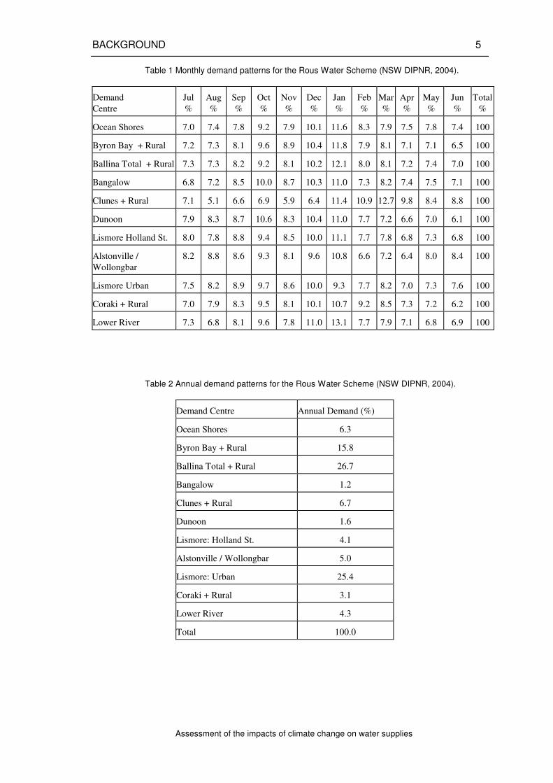
The monthly and annual demand patterns for the Rous Scheme are presented in Table 1 and
Table 2. The tables indicate that demand is relatively high during December and January, and
that Ballina and Lismore demand centres have the highest annual demand patterns. Ballina and
Lismore account for more than 25% of the total annual demand for the Rous Water scheme.
Figure 2 Domestic water use in Rous Water region.
BACKGROUND 5
Assessment of the impacts of climate change on water supplies
Table 1 Monthly demand patterns for the Rous Water Scheme (NSW DIPNR, 2004).
Demand
Centre
Jul
%
Aug
%
Sep
%
Oct
%
Nov
%
Dec
%
Jan
%
Feb
%
Mar
%
Apr
%
May
%
Jun
%
Total
%
Ocean Shores 7.0 7.4 7.8 9.2 7.9 10.1 11.6 8.3 7.9 7.5 7.8 7.4 100
Byron Bay + Rural 7.2 7.3 8.1 9.6 8.9 10.4 11.8 7.9 8.1 7.1 7.1 6.5 100
Ballina Total + Rural 7.3 7.3 8.2 9.2 8.1 10.2 12.1 8.0 8.1 7.2 7.4 7.0 100
Bangalow 6.8 7.2 8.5 10.0 8.7 10.3 11.0 7.3 8.2 7.4 7.5 7.1 100
Clunes + Rural 7.1 5.1 6.6 6.9 5.9 6.4 11.4 10.9 12.7 9.8 8.4 8.8 100
Dunoon 7.9 8.3 8.7 10.6 8.3 10.4 11.0 7.7 7.2 6.6 7.0 6.1 100
Lismore Holland St. 8.0 7.8 8.8 9.4 8.5 10.0 11.1 7.7 7.8 6.8 7.3 6.8 100
Alstonville /
Wollongbar
8.2 8.8 8.6 9.3 8.1 9.6 10.8 6.6 7.2 6.4 8.0 8.4 100
Lismore Urban 7.5 8.2 8.9 9.7 8.6 10.0 9.3 7.7 8.2 7.0 7.3 7.6 100
Coraki + Rural 7.0 7.9 8.3 9.5 8.1 10.1 10.7 9.2 8.5 7.3 7.2 6.2 100
Lower River 7.3 6.8 8.1 9.6 7.8 11.0 13.1 7.7 7.9 7.1 6.8 6.9 100
Table 2 Annual demand patterns for the Rous Water Scheme (NSW DIPNR, 2004).
Demand Centre Annual Demand (%)
Ocean Shores 6.3
Byron Bay + Rural 15.8
Ballina Total + Rural 26.7
Bangalow 1.2
Clunes + Rural 6.7
Dunoon 1.6
Lismore: Holland St. 4.1
Alstonville / Wollongbar 5.0
Lismore: Urban 25.4
Coraki + Rural 3.1
Lower River 4.3
Total 100.0

6
Assessment of the impacts of climate change on water supplies
Current supply
The Rous Water supply network includes over 30,000 connections within the reticulation areas
of the constituent Councils, and around 1,823 rural connections to the Rous Water trunk main
system. The system has adopted the former NSW Department of Public Works and Services
definition of ‘safe yield’ as the level of service to be provided by the Rous Water scheme.
Under this scheme the safe yield is defined as the annual demand that can be supplied from the
headworks over the period of record used in the analysis (i.e. 100-year duration) and which
satisfies the 5/10/20 rule (see Chapter 3 for detail).
Water presently comes from two main sources: Rocky Creek Dam and Emigrant Creek Dam.
The Rocky Creek Dam, which is situated 25 kilometres north of Lismore near the village of
Dunoon, has a storage capacity of 13,956 ML and a safe yield of about 9,600 ML/annum
(DIPNR, 2004). Emigrant Creek Dam was constructed in 1967–68 to provide a water supply to
Lennox Head and Ballina and is currently used to supplement the supply from Rocky Creek
Dam. Its capacity is 820 ML with a safe yield of about 1,100 ML/annum.
Other available sources under Council control include Convery’s Lane, Lumley Park and
Prospect Bores in the Ballina area, as well as three bores near Woodburn in the Richmond
Valley Shire. The combined safe yield is about 900 ML/annum.
The annual water production provided by the Rous Water Scheme from 1988 to 2004 is
presented in Figure 3. Production ranges from approximately 10,000 to 13,000 ML/year with a
long term average of 11,300 ML. The long-term trend is increasing, even though there were
times when the production was very low compared to the long-term average. For example, low
production periods occurred in 1988 due to mains restrictions; in 1996 as an impact of a
demand management and user-pay system; and in 2003 due to water restrictions imposed to
manage a drought (Franklin, pers. comm., 2006). Through several consultations with the Rous
Water authority, it was decided that the historical data of 1996–2005 should be used in a trend
analysis, to construct a realistic projection of demand (see Figure 31). Based on these data, the
trend in the annual water production (which represents the actual demand) was estimated to
increase at a rate of approximately 91 ML per year.
1986 1988 1990 1992 1994 1996 1998 2000 2002 2004 2006
An
nu
al w
ate
r p
rod
ucti
on
(M
L)
9000
9500
10000
10500
11000
11500
12000
12500
13000
Figure 3 Annual water production of Rous Water Scheme from 1988 to 2005.
BACKGROUND 7
Assessment of the impacts of climate change on water supplies
2.1.2 Future demand and supply
Future demands
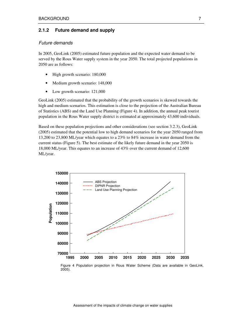
In 2005, GeoLink (2005) estimated future population and the expected water demand to be
served by the Rous Water supply system in the year 2050. The total projected populations in
2050 are as follows:
• High growth scenario: 180,000
• Medium growth scenario: 148,000
• Low growth scenario: 121,000
GeoLink (2005) estimated that the probability of the growth scenarios is skewed towards the
high and medium scenarios. This estimation is close to the projection of the Australian Bureau
of Statistics (ABS) and the Land Use Planning (Figure 4). In addition, the annual peak tourist
population in the Rous Water supply district is estimated at approximately 43,600 individuals.
Based on these population projections and other considerations (see section 3.2.3), GeoLink
(2005) estimated that the potential low to high demand scenarios for the year 2050 ranged from
13,200 to 23,800 ML/year which equates to a 23% to 84% increase in water demand from the
current status (Figure 5). The best estimate of the likely future demand in the year 2050 is
18,000 ML/year. This equates to an increase of 43% over the current demand of 12,600
ML/year.
1995 2000 2005 2010 2015 2020 2025 2030 2035
Po
pu
lati
on
70000
80000
90000
100000
110000
120000
130000
140000
150000
ABS Projection
DIPNR Projection
Land Use Planning Projection
Figure 4 Population projection in Rous Water Scheme (Data are available in GeoLink, 2005).

8
Assessment of the impacts of climate change on water supplies
2000 2005 2010 2015 2020 2025 2030 2035
An
nu
al d
em
an
d (
ML
)
12000
13000
14000
15000
16000
17000
18000
19000
20000
Low growth & consumption scenario
Best estimate demand
High growth & consumption scenario
Figure 5 Annual demand projections for Rous Water Scheme (Data are taken from GeoLink, 2005).
Future supply
Rous Water’s strategy, which was adopted in 1995 and amended in 2004, provides a range of
options to meet water requirements. These options include:
• investigate and develop alternative water resources such as reuse, where appropriate;
• implement demand management measures;
• develop the Lismore source; and
• develop Dunoon dam.
A key objective of Rous Water’s management plan is to implement effective demand
management principles under best practice guidelines. The performance target for this objective
is a minimum 10% reduction in the demand for water by the year 2011, relative to 1995
consumption levels (Rous Water, 2004). To achieve this objective, Rous Water has actively
promoted a variety of demand management initiatives. These include the Residential House
Tune-up Program, the Every Drop Counts–Primary School Education Program, the Rainwater
Tank Rebate Program, and the Washing Machine Rebate Program. These initiatives were
successful by several measures, but demand management alone may not solve the increasing
needs for water as the population grows (Rous Water, 2004).
The Lismore source and the Dunoon Dam were identified by the strategy as being essential in
expanding the capacity to meet future demand. The Lismore source is a medium-term solution

BACKGROUND 9
Assessment of the impacts of climate change on water supplies
which is able to assist in meeting the high demand projection up to year 2024. This will consist
of a pump station abstracting up to 30 ML/day of water from the upper reaches of the tidal pool
in the Wilson River, which would only occur when Rocky Creek Dam is below 95% capacity.
The point of abstraction will be about 5km upstream of Lismore (Howard’s Grass). The
Lismore Source is expected to increase the secure yield to 14,900 ML/year (Siebert and
Franklin, pers. comm., 2006).
The Dunoon Dam would store inflows from its catchment up to the existing Rocky Creek Dam
and from spills over the Rocky Creek Dam spillway (CMPS&F, 1995). Water drawn from
Dunoon Dam will be treated by a process similar to the process to be used at Nightcap Water
Treatment Plant after the present process improvement works are complete. Treated water will
be pumped to the existing distribution system near Dorroughby where it will flow by gravity to
Lismore. Alternatively, flow will be released into Rocky Creek to be abstracted from the
Wilson River at the Lismore Source for treatment and pumping to the existing distribution
system (CMPS&F, 1995).
These strategies were developed with an assumption that the climate remains unchanged. As
the following section describes, there is increasing evidence that the climate has changed, and
that the change may have an impact on future water availability. Therefore, it is necessary to
take this into account in the water management plan.
2.2 Climate Change
The climate of New South Wales (NSW) is generally mild and temperate. However, extremely
high daytime temperatures occur in the west during summer and extremely cold overnight
temperatures occur in the tablelands and dry western slopes of NSW during winter (Hennessy
et al, 2004). In the North-east, where the Rous Water area is located, average annual
temperatures are around 15–18°C, while the average annual rainfall is around 1,200 to 2,000
mm. Regional annual rainfall, measured as the annual 10th percentile, median and 90
th
percentile values, exceeds 800 mm, 1200 mm, and 2000 mm respectively (Hennessy, et al,
2004).
The present CO2 concentration of about 375 ppm is now higher than at any time in the past
740,000 years (EPICA, 2004). According to WMO (2003), the global average surface
temperature has risen by about 0.6°C since 1990, with the warmest year being 1998, followed
by 2002 and 2003. Computer models of the climate system have been used to estimate the
relative contributions of various factors such as changes in solar radiation, aerosols from
volcanic eruptions, increased greenhouse gas and aerosol emissions, stratospheric ozone
depletion, and internal climate variability from events like El Niño (Hennessy et al, 2004).
Most studies agree that global warming in the early 20th century can be explained by a
combination of natural and human-induced factors (IPCC, 2001a). IPCC (2001a, b) concluded
that:
• an increasing body of observations gives picture of a warming world and other changes
in the climate system;
• emissions of greenhouse gases and aerosols due to human activities continue to alter
the atmosphere in ways that affect the climate system;
10
Assessment of the impacts of climate change on water supplies
• there is new and stronger evidence that most of the warming observed over the last 50
years is attributable to human activities;
• recent climate changes have already affected many physical and biological systems;
and
• some human systems have been affected by recent increases in floods and droughts.
2.2.1 Historical climate patterns
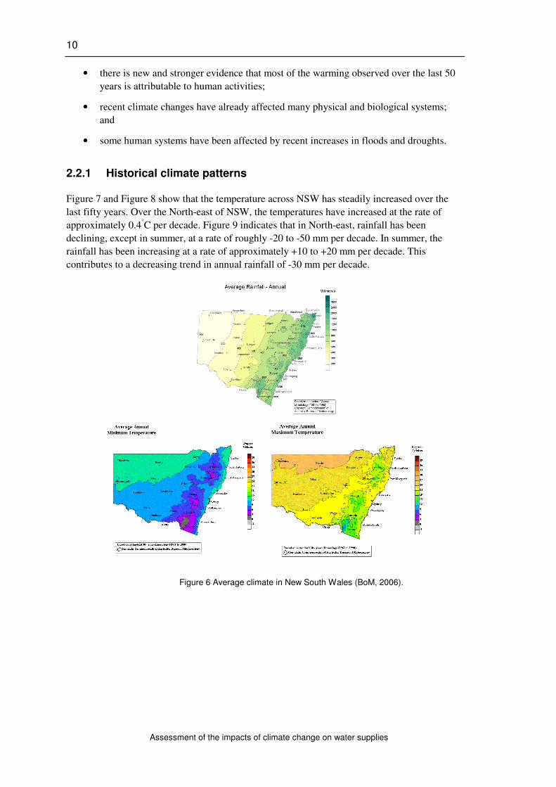
Figure 7 and Figure 8 show that the temperature across NSW has steadily increased over the
last fifty years. Over the North-east of NSW, the temperatures have increased at the rate of
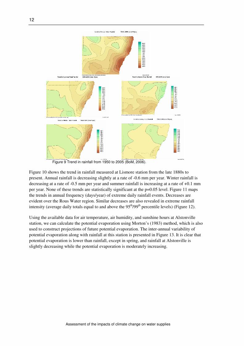
approximately 0.4°C per decade. Figure 9 indicates that in North-east, rainfall has been
declining, except in summer, at a rate of roughly -20 to -50 mm per decade. In summer, the
rainfall has been increasing at a rate of approximately +10 to +20 mm per decade. This
contributes to a decreasing trend in annual rainfall of -30 mm per decade.
Figure 6 Average climate in New South Wales (BoM, 2006).

BACKGROUND 11
Assessment of the impacts of climate change on water supplies
Figure 7 Trend in maximum temperature from 1950 to 2005 (BoM, 2006).
Figure 8 Trend in minimum temperature from 1950 to 2005 (BoM, 2006).
12
Assessment of the impacts of climate change on water supplies
Figure 9 Trend in rainfall from 1950 to 2005 (BoM, 2006).
Figure 10 shows the trend in rainfall measured at Lismore station from the late 1880s to
present. Annual rainfall is decreasing slightly at a rate of -0.6 mm per year. Winter rainfall is
decreasing at a rate of -0.5 mm per year and summer rainfall is increasing at a rate of +0.1 mm
per year. None of these trends are statistically significant at the p=0.05 level. Figure 11 maps
the trends in annual frequency (days/year) of extreme daily rainfall events. Decreases are
evident over the Rous Water region. Similar decreases are also revealed in extreme rainfall
intensity (average daily totals equal to and above the 95th/99
th percentile levels) (Figure 12).
Using the available data for air temperature, air humidity, and sunshine hours at Alstonville
station, we can calculate the potential evaporation using Morton’s (1983) method, which is also
used to construct projections of future potential evaporation. The inter-annual variability of
potential evaporation along with rainfall at this station is presented in Figure 13. It is clear that
potential evaporation is lower than rainfall, except in spring, and rainfall at Alstonville is
slightly decreasing while the potential evaporation is moderately increasing.

BACKGROUND 13
Assessment of the impacts of climate change on water supplies
y = -0.5732x + 1371.7
0
500
1000
1500
2000
2500
1884 1899 1914 1929 1944 1959 1974 1989 2004
Rain
fall (
mm
)
Annual
y = -0.4856x + 260.86
0
100
200
300
400
500
600
700
800
900
1884 1899 1914 1929 1944 1959 1974 1989 2004
Rain
fall (
mm
)
Winter
y = 0.1129x + 451.98
0
200
400
600
800
1000
1200
1400
1884 1899 1914 1929 1944 1959 1974 1989 2004
Rain
fall (
mm
)
Summer
Lismore
Figure 10 Rainfall in Lismore from the 1880s (source: current study).
Figure 11 Trend in frequency of extreme rainfall (Hennessy et al., 2004).
Figure 12 Trend in intensity of extreme rainfall (Hennessy et al., 2004).

14
Assessment of the impacts of climate change on water supplies
0
500
1000
1500
2000
2500
3000
3500
1970 1975 1980 1985 1990 1995 2000 2005R
ain
fall
(m
m)
0
500
1000
1500
2000
2500
3000
3500
Po
ten
tia
l E
va
po
rati
on
(m
m)
Rainfall Potential Evaporation
ANNUAL
0
200
400
600
800
1000
1200
1400
1600
1970 1975 1980 1985 1990 1995 2000 2005
Ra
infa
ll (
mm
)
0
200
400
600
800
1000
1200
1400
1600
Po
ten
tia
l E
vap
ora
tio
n (
mm
)
Rainfall Potential Evaporation
Summer
0
200
400
600
800
1000
1200
1400
1600
1970 1975 1980 1985 1990 1995 2000 2005
Ra
infa
ll (
mm
)
0
200
400
600
800
1000
1200
1400
1600
Po
ten
tial E
vap
ora
tio
n (
mm
)
Rainfall Potential Evaporation
Autumn
0
200
400
600
800
1000
1200
1400
1600
1970 1975 1980 1985 1990 1995 2000 2005R
ain
fall (
mm
)0
200
400
600
800
1000
1200
1400
1600
Po
ten
tial
Ev
ap
ora
tio
n (
mm
)
Rainfall Potential Evaporation
Winter
0
200
400
600
800
1000
1200
1400
1600
1970 1975 1980 1985 1990 1995 2000 2005
Ra
infa
ll (
mm
)
0
200
400
600
800
1000
1200
1400
1600
Po
ten
tial E
va
po
rati
on
(m
m)
Rainfall Potential Evaporation
Spring
Figure 13 Rainfall and potential evaporation in Alstonville along with their linear trend lines (Source: current study).
2.2.2 Projected climate change
The climate system is highly complex, and therefore it is inappropriate to simply extrapolate
past trends to predict future conditions. To estimate future climate change, scientists have
developed scenarios. Scenarios are alternative pictures of how the future might unfold, with no
statement of probability. They are used to assess consequences, and thus to provide some basis
for policies that might influence future developments, or enable business or governments to
cope with the new situation when it occurs (Pittock, 2003). Such scenarios enable scientists to
set projections of future conditions derived on the basis of explicit assumptions. The IPCC
commissioned a range of scenarios of greenhouse gas and sulphate aerosols emissions up to the
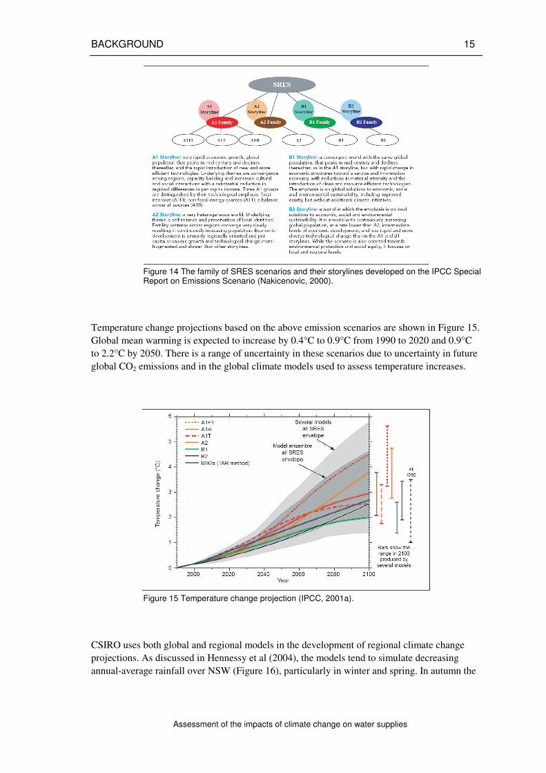
year 2100. The scenarios were reported in the Special Report on Emissions Scenarios (SRES).
The 40 SRES scenarios were based on four different ‘storylines’ of mutually consistent
development across different driving forces (Figure 14).
BACKGROUND 15
Assessment of the impacts of climate change on water supplies
Figure 14 The family of SRES scenarios and their storylines developed on the IPCC Special Report on Emissions Scenario (Nakicenovic, 2000).
Temperature change projections based on the above emission scenarios are shown in Figure 15.
Global mean warming is expected to increase by 0.4°C to 0.9°C from 1990 to 2020 and 0.9°C
to 2.2°C by 2050. There is a range of uncertainty in these scenarios due to uncertainty in future
global CO2 emissions and in the global climate models used to assess temperature increases.
Figure 15 Temperature change projection (IPCC, 2001a).
CSIRO uses both global and regional models in the development of regional climate change
projections. As discussed in Hennessy et al (2004), the models tend to simulate decreasing
annual-average rainfall over NSW (Figure 16), particularly in winter and spring. In autumn the

16
Assessment of the impacts of climate change on water supplies
direction of the change is uncertain, while in summer there is a tendency for increases in the
north-east.
Annual-average potential evaporation is projected to increase across NSW (Figure 17). The
largest changes are projected in winter with the smallest changes in summer, because baseline
potential evaporation rates are low in winter and high in summer. Compared to changes in the
other areas of NSW, projected changes in the north-east are relatively small.
Figure 16 Ranges of change in average rainfall (%) for the years 2030 and 2070 relative to 1990. The coloured bars show ranges of change for areas with corresponding colours in the maps. The reduction in the range is also shown for the IPCC’s 550 ppm and 450 ppm CO2 stabilisation scenarios (Hennessy et al., 2004).
Figure 17 Ranges of change in point potential evaporation (%) for the years 2030 and 2070 relative to 1990. The coloured bars show ranges of change for areas with corresponding colours in the maps. The reduction in the range is also shown for the IPCC’s 550 ppm and 450 ppm CO2 stabilisation scenarios (Hennessy et al., 2004).
BACKGROUND 17
Assessment of the impacts of climate change on water supplies
2.2.3 Potential impact on water supply and demand
Impacts on water supply
The relationship between climate, water supply and demand is relatively complex. Therefore,
estimating the impact of climate change on water demand and water supply is not a simple task.
Some estimates of changes in runoff due to climatic change have been produced using
hydrologic models and a variety of climate scenarios in Australia. In general, these studies
indicate that climate change may reduce runoff, streamflow and water supply.
CSIRO and Melbourne Water, for instance, recently completed a joint study of climate change
risks to Melbourne’s water supply (Howe et al. 2005). The risks that were identified include:
• Water Supply
• reduced water supply due to lower streamflow;
• bushfires in catchment areas;
• pipe failure and collapse;
• Sewerage
• reduced environmental condition of streams;
• the potential for corrosion and odours in the sewerage network;
• sewer overflows during storms;
• Stormwater
• increased flooding risk and damage to stormwater infrastructure and facilities; and
• the potential for negative water quality impacts due to increased concentration of
pollutants entering the bay together with higher ambient bay water temperatures.
The study indicated that average inflow to Melbourne dams may decline 3–11% by 2020, and
7–35% by 2050 (Figure 18). The mid-range scenario indicated an 8% reduction in average
annual volume of water supplied to the system by 2020 rising to 20% by 2050. Another study
in Stirling Dam, Western Australia indicated that the current annual inflow of about 53.9 GL is
projected to decrease as much as 24% to 41.1 GL in 2042–2062 due to climate change (The
Department of Environment, 2004). In Adelaide, climate change may result in a reduction of
flows into reservoirs of as much as 17 GL per year (Water Proofing Adelaide, 2004).
Potential impacts of climate change on Rous Water Supply infrastructure are summarised in
Table 3. Decreasing yield from major sources and increasing competition with irrigators have
been expected. Climate change may also cause water quality problem, therefore water treatment
will be more expensive. In Emigrant Creek Dam, for instance, outbreaks of blue algae are
already common, and these may become worse in a warming world (Rous Water, 2006).

18
Assessment of the impacts of climate change on water supplies
Figure 18 Projected changes in water supply due to climate change in Greater Melbourne (Our Water Our Future, 2005).
Table 3 Potential impacts of climate change on Rous Water Supply Infrastructures (Summarised from Rous Water, 2006).
Potential impacts Changes in climate
Rocky
Creek Dam
Emigrant Creek
Dam
Lismore Source Dunoon Dam
Longer dry periods Yield to drop as
dam is small
relative to annual
extraction
Emptying dam needs to
be done on a regular
basis. Yield to drop due
to a longer period
between replenishment
Pumping will cease
earlier in the year to
maintain environmental
flows. Longer period of
time without extraction
from source
Possibly some loss of
yield compared from
previous estimates
but larger capacity
dam should fare
better
Increased
evaporation
Yield to drop as
more water is lost
to the atmosphere
and longer periods
transpire without
inflow
Yield to drop as more
water is lost to the
atmosphere and longer
periods transpire
without inflows. Very
high surface area to
volume ratio
Irrigation demand rises,
increasing competition
with irrigators
Expected loss of
yield compared to
previous estimates
Higher water
temperature
Greater water
quality problems
Greater water quality
problems
Higher incidence of
algae. Not a current
problem
Expect similar water
quality problems in
Rocky Creek Dam
Intensity of rainfall High treatment cost due
to turbid inflow and
perhaps some loss of
throughput
Higher turbidity but not
necessarily for longer
periods of time
BACKGROUND 19
Assessment of the impacts of climate change on water supplies
Impacts on water demand
Unlike the impacts of climate change on water supply, studies of the impact of climate change
on water demand are rather limited. Most of the available demand analysis is focused on the
impact of demand management and population growth (e.g. Figure 5). The estimation of the
impact of climate change on water demand is rather complicated since the demand is not only
influenced by climatic factors but also by socioeconomic factors (e.g. demography, economy,
land use, culture, and infrastructure); policy (e.g. regulation, and investment); and stakeholder
decision-making (e.g. business strategy, responds to risk, and planning guidelines). In addition,
water demand can be divided into several sectors such as domestic, agriculture, leisure, and
industry. Each sector has different sensitivities to climate change. For example, in the domestic
sector, people generally spend more time in their garden and have fountains to cool patios by
evaporation in warmer weather. However, in the Rous Water region, outdoor water demand
(31%) is much less compared to that of the typical households in Australia (60%), therefore the
outdoor water demand in this region will be less affected by climate change.
Empirical information on the impact of climate change on Rous Water’s water demand was
limited at the time of this project. However, some relevant knowledge of other regions close to
the Rous Water can be used as surrogates. For instance, a water-demand analysis in
Queensland’s urban community has indicated that it is the frequency of rainfall, not the amount
that significantly affects the external use of water in Maroochy, Mackay, and Ingham, whereas
the amount of rainfall and the monthly air temperature are the most significant variables
affecting water demand in the inland communities of Toowoomba and Emerald (Montgomery
Watson, 2000).

20
Assessment of the impacts of climate change on water supplies
3. FRAMEWORK FOR IMPACT ASSESSMENT
3.1 Introduction
Most research on the hydrologic impact of climate change uses a predictive approach. It begins
with generating climate change scenarios. Climate information is then fed into hydrologic
models and/or water-management systems to evaluate the differences in system performance
under different climate scenarios. Adaptations can then be designed to manage those changes.
There are large uncertainties in these scenarios, arising from estimates of global greenhouse
emissions, global climate sensitivity, regional changes, and climate variability. Hydrologic
models also contain modelling uncertainty. In addition, climate change is just one of a number
of factors putting pressure on the hydrological system and water resources. Population growth,
changes in land use, water policies, prices, and adaptation are just a few examples of other
factors affecting the water supply and demand. Therefore, the above predictive approach is
limited by scenario uncertainty and often neglects the relationship between current climate risk,
vulnerability to that risk and adaptations developed to manage risk. To deal with uncertainty, it
is suggested that climate change and its consequences should be expressed in units of
probability or likelihood. This enables one to pursue risk-based impact assessment and
management, whereby thresholds for climatic changes and/or specific impacts are integrated
with probability distributions for climate, environmental, and socioeconomic variables that
influence system outcomes (Jones, 2001). Also, to deal with the dynamics of the system,
assessing the impacts of climate change cannot be a static activity. Hence, new information is
constantly being made available, new methods and models are being developed and tested, and
policies related to water management and planning are dynamic and changing (Gleick and
Adams, 2000).
Impact and risk assessment is only one stage in a larger risk management framework (Kirono et
al., 2006). Ideally, risk management involves all related stakeholders. The decision-making
process is commonly circular to allow the performance of decisions taken to be reviewed and
revisited as new information on climate change and its impacts are available. It is also iterative
to allow the problem, decision-making criteria, risk assessment and adaptation options to be
refined.
Through consultation with stakeholders at the workshop on the 7th of April 2006 and regular
fortnightly communications, the following key issues were identified for the risk analysis and
adaptation assessment:
• Rous Water needs to know when to make infrastructure investments;
• a minimum of ten years is required to commission a new water source;
• it is agreed to use Wilson River IQQM FX94D as the baseline (see section 3.2.4 for
information about model);
• the assessment endpoint is the secure yield. The secure yield is defined as the annual
demand that can be supplied over the period of record used in the analysis (i.e. 100 year

FRAMEWORK FOR IMPACT ASSESSMENT 21
Assessment of the impacts of climate change on water supplies
duration) and which satisfies the 5/10/20 rule which is commonly applied by the NSW
Public Works to determine the safe yield from a dam (Rous Water, 1995):
• restrictions of any kind should not be applied for more than 5% of the time (i.e. 5%
days);
• restrictions of any kind should not be imposed more than one year in ten on average
(i.e. 10% years); and
• the system should be able to supply 80% of normal demand (i.e. 20% reduction in
consumption) through a repeat of the worst drought on record. The system should
start with the storage drawn down to a level at which restrictions should be applied
in-order to satisfy the above 5% and 10% rules (this known as the 20% part of the
rule). Note that this was modelled by changing dam capacity to 80% and imposing
permanent restrictions and ensuring the demand was met through the worst drought
in the 100 year record.
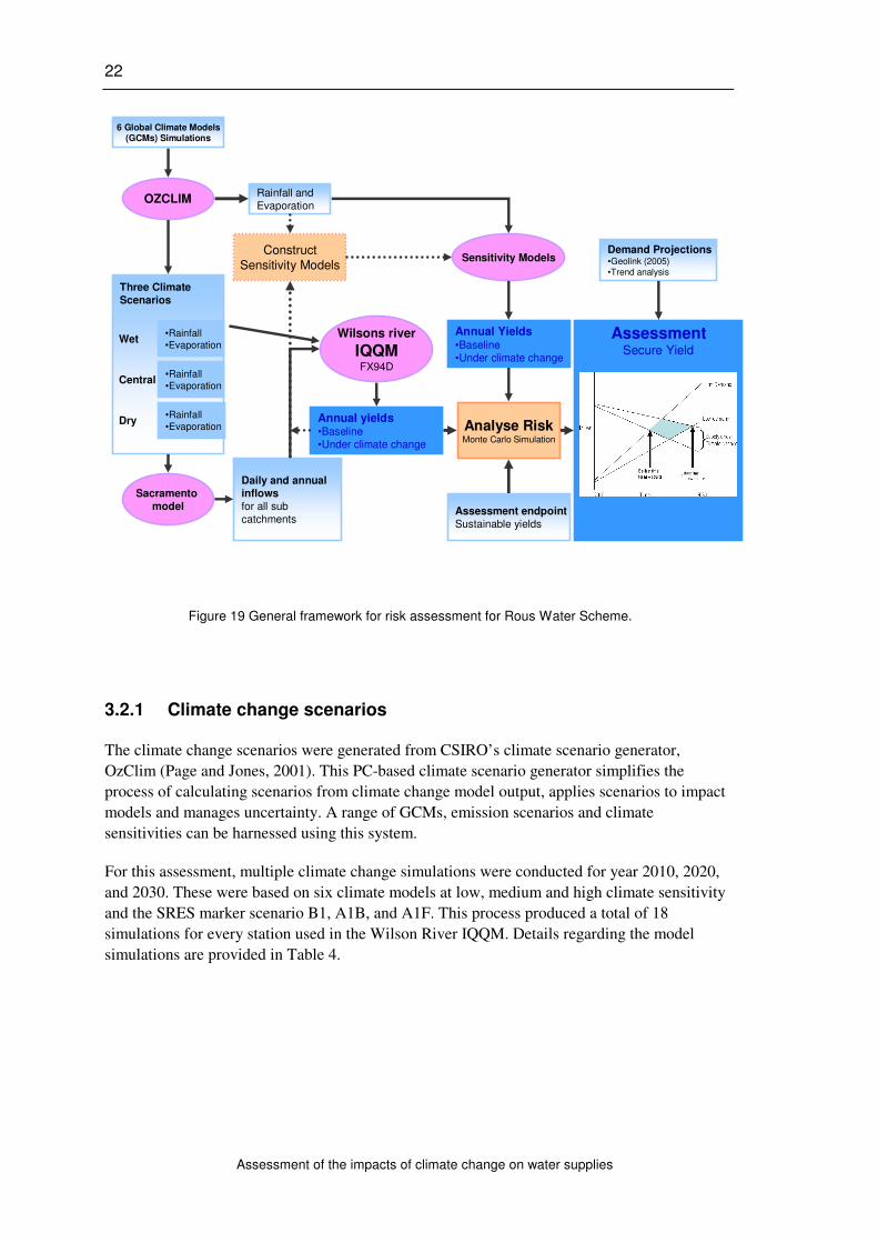
3.2 Risk assessment
Figure 19 presents the assessment framework for climate change impacts and adaptation. The
framework follows the following main steps:
• Select six Global Climate Model (GCM) simulations through the use of the
CSIRO Climate Scenario generator, OzClim;
• Prepare three climate scenarios (one wet, one medium, one dry) expressed as a
function of global warming (percent change per oC of global warming) for
potential evaporation (Ep) and precipitation (P) for specified times in the future
(2010, 2020, 2030) for each of the six GCMS. This results in a total of 18 climate
scenarios;
• Apply these climate scenarios in the IQQM model to generate climate change
flow sequences. Rainfall and evaporation inputs to IQQM are modified to
simulate climate change;
• Analyse the sensitivity of secure yields to changes in inflow to Rocky Creek dam,
Emigrant Creek dam, and the downstream tributary via a large number of IQQM
simulations. This generates sensitivity models which can be used to estimate
yields based on evaporation and rainfall changes;
• Analysis the risks to Lismore’s future water supply yield and secure yield by
using Monte Carlo methods (repeated random sampling);
• Evaluate risk and identify feedbacks likely to result in autonomous adaptations;
and
• Consult with stakeholders, analyse proposed adaptations and recommend planned
adaptation options.
Details about how these tasks were performed are provided in section 3.2.1 to section 3.2.4.
22
Assessment of the impacts of climate change on water supplies
OZCLIM
Wilsons river
IQQMFX94D
Demand Projections•Geolink (2005)•Trend analysis
Three Climate
Scenarios
•Rainfall•Evaporation
•Rainfall•Evaporation
•Rainfall•Evaporation
Wet
Central
Dry
Assessment endpoint
Sustainable yields
Analyse RiskMonte Carlo Simulation
AssessmentSecure Yield
Annual yields•Baseline
•Under climate change
6 Global Climate Models(GCMs) Simulations
Rainfall and
Evaporation
Sensitivity Models
Annual Yields•Baseline
•Under climate change
Sacramento
model
Daily and annual
inflows
for all sub
catchments
Construct
Sensitivity Models
Figure 19 General framework for risk assessment for Rous Water Scheme.
3.2.1 Climate change scenarios
The climate change scenarios were generated from CSIRO’s climate scenario generator,
OzClim (Page and Jones, 2001). This PC-based climate scenario generator simplifies the
process of calculating scenarios from climate change model output, applies scenarios to impact
models and manages uncertainty. A range of GCMs, emission scenarios and climate
sensitivities can be harnessed using this system.
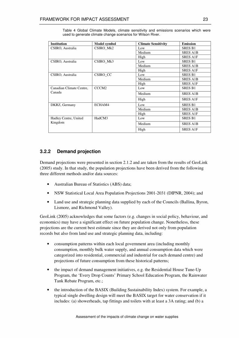
For this assessment, multiple climate change simulations were conducted for year 2010, 2020,
and 2030. These were based on six climate models at low, medium and high climate sensitivity
and the SRES marker scenario B1, A1B, and A1F. This process produced a total of 18
simulations for every station used in the Wilson River IQQM. Details regarding the model
simulations are provided in Table 4.
FRAMEWORK FOR IMPACT ASSESSMENT 23
Assessment of the impacts of climate change on water supplies
Table 4 Global Climate Models, climate sensitivity and emissions scenarios which were used to generate climate change scenarios for Wilson River.
Institution Model symbol Climate Sensitivity Emission
Low SRES B1
Medium SRES A1B
CSIRO, Australia CSIRO_Mk2
High SRES A1F
Low SRES B1
Medium SRES A1B
CSIRO, Australia CSIRO_Mk3
High SRES A1F
Low SRES B1
Medium SRES A1B
CSIRO, Australia CSIRO_CC
High SRES A1F
Low SRES B1
Medium SRES A1B
Canadian Climate Centre,
Canada
CCCM2
High SRES A1F
Low SRES B1
Medium SRES A1B
DKRZ, Germany ECHAM4
High SRES A1F
Low SRES B1
Medium SRES A1B
Hadley Centre, United
Kingdom
HadCM3
High SRES A1F
3.2.2 Demand projection
Demand projections were presented in section 2.1.2 and are taken from the results of GeoLink
(2005) study. In that study, the population projections have been derived from the following
three different methods and/or data sources:
• Australian Bureau of Statistics (ABS) data;
• NSW Statistical Local Area Population Projections 2001-2031 (DIPNR, 2004); and
• Land use and strategic planning data supplied by each of the Councils (Ballina, Byron,
Lismore, and Richmond Valley).
GeoLink (2005) acknowledges that some factors (e.g. changes in social policy, behaviour, and
economics) may have a significant effect on future population change. Nonetheless, these
projections are the current best estimate since they are derived not only from population
records but also from land use and strategic planning data, including:
• consumption patterns within each local government area (including monthly
consumption, monthly bulk water supply, and annual consumption data which were
categorized into residential, commercial and industrial for each demand centre) and
projections of future consumption from these historical patterns;
• the impact of demand management initiatives, e.g. the Residential House Tune-Up
Program, the ‘Every Drop Counts’ Primary School Education Program, the Rainwater
Tank Rebate Program, etc.;
• the introduction of the BASIX (Building Sustainability Index) system. For example, a
typical single dwelling design will meet the BASIX target for water conservation if it
includes: (a) showerheads, tap fittings and toilets with at least a 3A rating; and (b) a

24
Assessment of the impacts of climate change on water supplies
rainwater tank or alternative water supply for outdoor water use and toilet flushing
and/or laundry (DIPNR, 2005); and
• the implementation of dual reticulation schemes within the supply area. Dual
reticulation refers to the use of highly treated effluent (recycled water) for non-potable
uses at households.
In addition, a simple trend analysis was performed using the 1996–2005 historical data. This
analysis produced a tool to project future demand based upon available demand data (see also
section 2.1.1).
3.2.3 Yield estimation using IQQM
This study used the Integrated Quantity and Quality Model of the Wilsons River which is
described in detail in DIPNR (2004). The IQQM is a hydrologic, river system simulation
package for water resources planning purposes at the river basin scale (DLWC, 1998). IQQM
consists of the Sacramento rainfall-runoff model and river routing, water demand and allocation
routines to simulate river flow and regulation. This software has been implemented in most
regulated and a large number of unregulated river systems in NSW and Queensland.
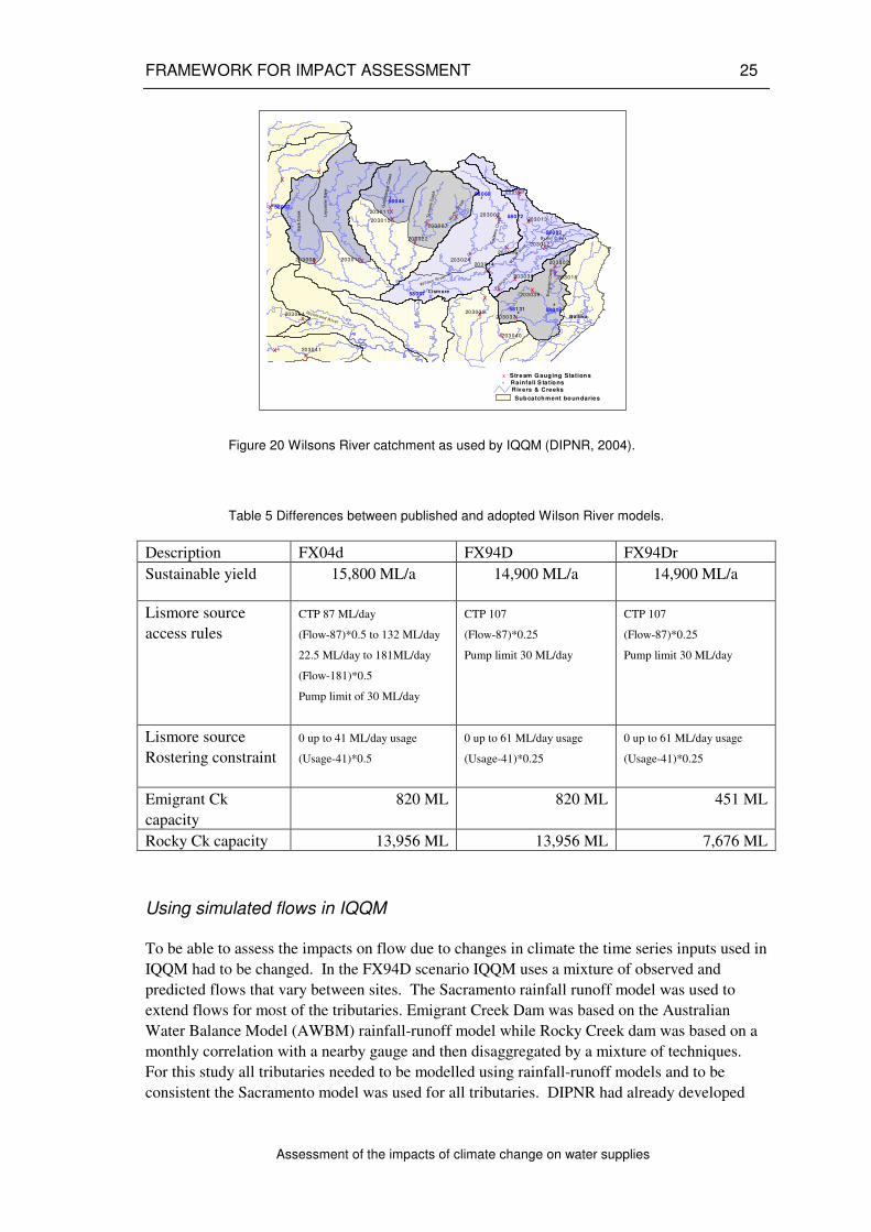
The Wilsons River catchment is shown in Figure 20 along with the climatic and hydrological
stations which are used in IQQM. The number of observed rainfall, evaporation, and stream
flow stations used in the model are 8, 1, and 14, respectively. Rainfall data is used to account
for soil moisture (which governs the crop water demands of irrigators) and to apply rainfall
onto the water surfaces of reservoirs and river reaches. Rainfall data is also required for
calculating catchment inflows. The evaporation data is used to estimate potential
evapotranspiration from crops, evaporation from reservoirs and river reaches, and to synthesize
streamflow.
The model incorporates existing irrigation development (3,000 ha); system demands (11
urban/rural demand centres); sources of supply (Rocky Creek Dam, Emigrant Creek Dam, and
Borefields); scheme operating rules and access to streamflows at Lismore.
The published results for the Wilsons River model (DIPNR, 2004) are based on a model
scenario known as FX04D. The Lismore source access rules have been investigated further,
resulting in a revised scenario known as FX94D, which is as yet unpublished. Based on a
discussion with Rous Water, this study has adopted the FX94D model run as the baseline from
which to assess the impacts of climate changes. The differences between the FX94D model
and the published FX04D model are presented in Table 5.
To assess the 20% rule a variation of the FX94D model has been created for this study
(FX94Dr). In this scenario the storages are configured to 55% capacity, which imposes
permanent water restrictions within the model. This is used to establish the baseline for the
5/10/20 rule.
FRAMEWORK FOR IMPACT ASSESSMENT 25
Assessment of the impacts of climate change on water supplies
#
#
#
#
# #
#
#
x
x
x
x
x
x x
x
x
x
x
x
x
x
x
x
x
x
x
x
x
x
x
x
x
x
x
xx
#
#
203041
203040
203039
203037
203022
203016
203015
203014
203013
203012
203011
203010203009
203007
203003
203002
203001
203046
58002
58018
58032
58037
58044
58060
58072
58131
Back
Cre
ek
Ley
cest
er
Riv
er
Goo
l ma n
gar
Cr e
ek
Te
r ran
ia C
r ee
k
Ro c
k y C
r eek
Co
oper s
Cr e
ek
Wils
on R
iver
Em
i gra
nt C
r eek
Byron C ree k
203038
Pea rc
e s Cre
ek
203024
Li sm ore
Ballina
W il son Ri ver
203004 Richm ond R iver
203039
Subcatchment boundaries
Rivers & Creeks
# Ra infall S ta tionsx Stream G auging Stations
Figure 20 Wilsons River catchment as used by IQQM (DIPNR, 2004).
Table 5 Differences between published and adopted Wilson River models.
Description FX04d FX94D FX94Dr
Sustainable yield 15,800 ML/a 14,900 ML/a 14,900 ML/a
Lismore source
access rules
CTP 87 ML/day
(Flow-87)*0.5 to 132 ML/day
22.5 ML/day to 181ML/day
(Flow-181)*0.5
Pump limit of 30 ML/day
CTP 107
(Flow-87)*0.25
Pump limit 30 ML/day
CTP 107
(Flow-87)*0.25
Pump limit 30 ML/day
Lismore source
Rostering constraint
0 up to 41 ML/day usage
(Usage-41)*0.5
0 up to 61 ML/day usage
(Usage-41)*0.25
0 up to 61 ML/day usage
(Usage-41)*0.25
Emigrant Ck
capacity
820 ML 820 ML 451 ML
Rocky Ck capacity 13,956 ML 13,956 ML 7,676 ML
Using simulated flows in IQQM
To be able to assess the impacts on flow due to changes in climate the time series inputs used in
IQQM had to be changed. In the FX94D scenario IQQM uses a mixture of observed and
predicted flows that vary between sites. The Sacramento rainfall runoff model was used to
extend flows for most of the tributaries. Emigrant Creek Dam was based on the Australian
Water Balance Model (AWBM) rainfall-runoff model while Rocky Creek dam was based on a
monthly correlation with a nearby gauge and then disaggregated by a mixture of techniques.
For this study all tributaries needed to be modelled using rainfall-runoff models and to be
consistent the Sacramento model was used for all tributaries. DIPNR had already developed

26
Assessment of the impacts of climate change on water supplies
Sacramento models for Rocky Creek Dam and Emigrant Creek Dam that had a good match with
the short periods of observed data and these were adopted.
The Sacramento models generally matched well with observed flows at all sites. However,
when the observed data were replaced with the simulated data, the result for secure yield was
different to that from the original FX94D model. As the model is most sensitive to inflows
from Rocky Creek Dam and Emigrant Creek Dam, the Sacramento models for these tributaries
were adjusted until the original secure yield of 14,900 ML/year was achieved without
significantly changing the mass balance from the 100-year time series of simulated streamflow.
Unfortunately this was not quite possible due to very small differences (<2%) in critical events
for the to 5% and 10% rules. The best that could be achieved was a secure yield of 15,000
ML/year while keeping the difference in overall volume at Emigrant Ck and Rocky Ck within
2%. Consequently, for this study, all secure yields are compared against a baseline secure yield
of 15,000 ML/year rather than the 14,900 ML/year obtained in the DNR FX94D scenario.
Methodology for determining secure yield
Secure yield for the Rous Water supply was estimated based upon the minimum yield required
to meet the 5/10/20 rule (Section 3.1). Figure 21 shows the combined Rocky Ck and Emigrant
Creek storage volumes from 1892 to 2002 (110 years) for the FX04D scenario. The figure
shows that the system is able to meet the secure yield for the 5% and 10% rules. According to
the 5% rule, restrictions of any kind should not be applied for more than 5% of the time. During
this time, restrictions had been applied for about 886 days, therefore less than 5% of the total
time (i.e., 2,021 of 40,436 days total). The supply was also able to meet the 10% rule as the
restrictions had been in place less than 11 years of the 110-year record.
date:27/04/06 t im e:09:24:29.45
Rous W ater
Total Supply Volume
01/01/1892 to 16/09/2002
0
2000
4000
6000
8000
10000
12000
14000
ML
Y ears
1900
1910
1920
1930
1940
1950
1960
1970
1980
1990
2000
Current volume
Restrictions
Dead storage
Figure 21 Rous water total supply generated from IQQM from 1890 to 2002.

FRAMEWORK FOR IMPACT ASSESSMENT 27
Assessment of the impacts of climate change on water supplies
The estimation of secure yield for each climate scenario required an iterative solution that
successively modifies and runs IQQM until the demand is met in accordance with the 5/10/20
rule. The iterative solution is described in Appendix 1.
This process is carried out for each of the climate scenarios, for a total of 54 scenarios (i.e., 18
scenarios for each of the years 2010, 2020 and 2030). To solve each scenario, IQQM was run
approximately 10 times, resulting in approximately 540 runs to cover all of the climate
scenarios.
3.2.4 Yields under climate change
For impact assessment, the estimated yields under climate change were based on the IQQM
output. In this case (referred to as IQQM), OzClim was used to generate daily records of
rainfall (P) and evaporation (Ep) for each climate change scenario. These modified records
were then input to the IQQM Sacramento model to generate climate change flow sequences.
The rainfall, evaporation and flow records within IQQM were replaced with the modified
climate change records. IQQM was run to apply multiple scenarios for 2010, 2020, and 2030.
By doing so, we obtained multiple estimates of the yield at Lismore and the yield of the whole
system for each of these years.
In addition, to explore the potential of having a very simple model which can provide a simple
and quick estimate of change in yield to a given change in climate, this project developed
simple model which enables one to estimate change in yield as a function of changes in rainfall
and evaporation. The approach (here referred to as the sensitivity model) involves the use of
two sets of transfer functions: one set relates precipitation and evaporation to inflows, the other
relates inflows to yields. To do this, the relationships between climate and inflows of the main
sources (i.e. Rocky Creek Dam, Emigrant Creek Dam, and downstream tributaries) were first
examined. The results (not shown here) suggest that all inflows show the same sensitivity to
changes in rainfall. For instance, approximately 10% change in rainfall results in about 15%
change in inflow.
These actions produced a simple multivariate transfer function relating the inflow with P and
Ep to estimate inflow of each main source using the input of P and Ep. The multi-linear
function of the model is as follows:
Flow = (a × P) + (b × Ep) – c
Where P and Ep were measured in mm per year and inflow in ML per year, and a, b, and c are
constants.
Figure 22 shows that the above transfer function is quite capable of estimating the inflow.
Quantitatively, the standard errors of estimates from the model were 2%, 5%, and 8% for the
Rocky Creek Dam, the Emigrant Creek Dam, and the downstream tributary, respectively. These
model validations suggest that the sensitivity models can be confidently used to estimate flow
as a function of P and Ep.
Sensitivity tests were subsequently conducted to assess the sensitivity of the secure yields to
inflow of the main source (i.e. Rocky Creek Dam, Emigrant Creek Dam, and downstream

28
Assessment of the impacts of climate change on water supplies
tributary). To do this, the IQQM was run several times to assess the impact of the following
assumptions on the secure yields:
• ±1%, ±2%, ±5%, and −10% changes in inflows; and
• +10% changes in irrigation demand (which is conducted by adjusting the area).
Figure 23 presents the changes in secure yields due to changes in inflow of each source. It
suggests that the secure yields are mostly sensitive to flows downstream of the dams as they
influence the amount of water abstracted at Lismore. These analyses also demonstrated that the
secure yields are not sensitive to changes in the irrigation demand (not shown here).
The results of these sensitivity analyses were then utilised to develop the other transfer function
that can provide estimates of secure yields as a function of inflow to the Rocky Creek dam,
Emigrant Creek dam, and the downstream tributaries.
0
20000
40000
60000
80000
100000
1890 1900 1910 1920 1930 1940 1950 1960 1970 1980 1990 2000
Flo
w (M
L)
observed RockyCk modelled RockyCk
0
20000
40000
60000
80000
1890 1900 1910 1920 1930 1940 1950 1960 1970 1980 1990 2000
Flo
w (M
l)
Observed Emigrant Cr Modelled Emigrant Cr
0
20000
40000
60000
80000
1890 1900 1910 1920 1930 1940 1950 1960 1970 1980 1990 2000
Flo
w (M
l)
Observed Downstream Modelled Downstream
Figure 22 Comparison between the observed and the modelled inflow of each main source.

FRAMEWORK FOR IMPACT ASSESSMENT 29
Assessment of the impacts of climate change on water supplies
-5
-3
-1
1
3
5
-12 -10 -8 -6 -4 -2 0 2 4 6 8 10 12
Changes in flow (%)
Ch
an
ge
s in
sys
tem
yie
lds
(%
)
Rocky Creek Emigrant Creek Downstream Tributary
Figure 23 Changes in secure yields due to changes in inflow of each main source.
3.3 Risk Analysis
As mentioned previously, the issue of climate change is beset by uncertainties. These
uncertainties include the magnitude of global warming, regional changes in rainfall and
evaporation, and regional supply sensitivity and coping capacity. In the face of this problem,
quantifying the uncertainties in climate change and its downstream consequences in units of
probability or likelihood will help identify robust adaptation strategies.
There are two types of likelihood for future events that are both measured in terms of
probability:
• event-based probability where the likelihood of recurring events is estimated (e.g.
floods, droughts and temperature extremes).
• the probability of a specific outcome which is measured over a range of future
uncertainty.
In this study, the second type of probability is used to describe the future state of climate
change under the enhanced greenhouse effect. To do this, Monte Carlo methods (repeated
random sampling) were employed to stochastically generate probabilistic estimates of future
climate change and its impacts on Rous Water’s secure yields.
To estimate the probability of climate change, three types of uncertainty are taken into account:
• future greenhouse gas and sulphate aerosol concentrations;
• the sensitivity of climate to these concentrations; and
• regional patterns of climate change from different climate models.
These uncertainties are quantified as ranges with an upper and lower limit and a known
probability distribution. These ranges are then randomly sampled repeatedly and combined to
30
Assessment of the impacts of climate change on water supplies
determine a joint probability distribution relevant to the secure yields. The Monte Carlo
sampling was conducted for 2010, 2020, and 2030 in the following manner:
Random local P change = Random global warming × Random local P change per oC global warming
Random local Ep change = Random global warming × Random local Ep change per oC global warming
This random sampling was repeated 2,500 times in year 2010, 2020, and 2030 to get an
adequate sampling density over the projected range of uncertainty. Simulations samples were
subsequently used to calculate cumulative probability distributions for future climates as shown
in Chapter 4 (e.g. Figure 24 and Figure 25).

RISK ANALYSIS RESULTS 31
Assessment of the impacts of climate change on water supplies
4. RISK ANALYSIS RESULTS
4.1 Climate Change Probabilities
The probability of the most to the least likely future climates is shown in Figure 24 and Figure
25. These cumulative probability graphs rank the data in the simulation from the highest to the
lowest value, and graph each point with its corresponding percentile. This treats each outcome
as being of equal likelihood. For example, in 2030 there is a 20% probability that the change in
evaporation will be +23% or less (Figure 24) and there is a 50% probability that the change in
Rocky Creek rainfall will be about -5% in 2030 (Figure 25). The downward sloping cumulative
probability graphs indicate the proportion of data in the simulation predicted to exceed each
value on the x-axis. The inspection of both figures suggests the following:
• Increases in potential evaporation are virtually certain (i.e. >99% probability of
occurrence). The 95th and 5
th outcomes range from about 2% to 4% in 2010, 4% to
12% in 2020, and 10% to 26% in 2030.
• The chances of decreasing rainfall are relatively even with the chances of increasing
rainfall, particularly in the downstream tributary area. The lowest and highest (5th
and 95th) changes in P range from about 2% to −4% in 2010, 7% to −11% in 2020,
and 17% to −21% in 2030.
Evaporation change (%)
0 10 20 30 40
Cu
mu
lative
pro
ba
bili
ty (
%)
0
20
40
60
80
100
2010
2020
2030
There is a 20% probability that the change in evaporation is +23% or less
Figure 24 Probability distributions for evaporation changes in 2010, 2020, and 2030. An example about how to interpret this graph is provided for year 2030.

32
Assessment of the impacts of climate change on water supplies
Rocky Creek
Rainfall change (%)
-40 -20 0 20 40
Cum
ula
tive p
rob
ab
ility
(%
)
0
20
40
60
80
100
2010
2020
2030
Emigrant Creek
Rainfall change (%)
-40 -20 0 20 40
Cum
ula
tive p
roba
bili
ty (
%)
0
20
40
60
80
100
Downstream Tributary
Rainfall change (%)
-40 -20 0 20 40
Cu
mula
tive p
roba
bili
ty (
%)
0
20
40
60
80
100
There is a 50% probability that rainfall will decrease by 5%
Figure 25 Probability distribution for rainfall changes in 2010, 2020, and 2030. Example about how to interpret this graph is provided for Rocky Creek dam rainfall in 2030.
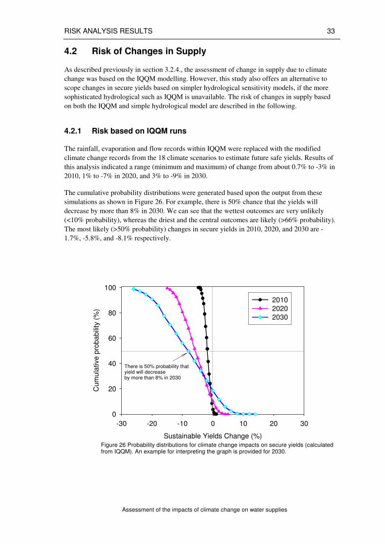
RISK ANALYSIS RESULTS 33
Assessment of the impacts of climate change on water supplies
4.2 Risk of Changes in Supply
As described previously in section 3.2.4., the assessment of change in supply due to climate
change was based on the IQQM modelling. However, this study also offers an alternative to
scope changes in secure yields based on simpler hydrological sensitivity models, if the more
sophisticated hydrological such as IQQM is unavailable. The risk of changes in supply based
on both the IQQM and simple hydrological model are described in the following.
4.2.1 Risk based on IQQM runs
The rainfall, evaporation and flow records within IQQM were replaced with the modified
climate change records from the 18 climate scenarios to estimate future safe yields. Results of
this analysis indicated a range (minimum and maximum) of change from about 0.7% to -3% in
2010, 1% to -7% in 2020, and 3% to -9% in 2030.
The cumulative probability distributions were generated based upon the output from these
simulations as shown in Figure 26. For example, there is 50% chance that the yields will
decrease by more than 8% in 2030. We can see that the wettest outcomes are very unlikely
(<10% probability), whereas the driest and the central outcomes are likely (>66% probability).
The most likely (>50% probability) changes in secure yields in 2010, 2020, and 2030 are -
1.7%, -5.8%, and -8.1% respectively.
Sustainable Yields Change (%)
-30 -20 -10 0 10 20 30
Cum
ula
tive
pro
ba
bili
ty (
%)
0
20
40
60
80
100
2010
2020
2030
There is 50% probability that yield will decrease by more than 8% in 2030
Figure 26 Probability distributions for climate change impacts on secure yields (calculated from IQQM). An example for interpreting the graph is provided for 2030.

34
Assessment of the impacts of climate change on water supplies
4.2.2 Based on sensitivity models
The climate-inflows transfer functions obtained in section 3.2.4 were used to estimate changes
in inflow to the main sources (Rocky Creek Dam, Emigrant Creek Dam, and downstream
tributaries) due to changes in rainfall and evaporation based upon the 18 climate scenarios in
2010, 2020, and 2030. Subsequently, these estimated inflows are input to the inflow-yield
transfer function to estimate changes in the yields in each future year.
Figure 27 presents cumulative probability distributions for changes in yields where the
probability distribution is tallied from wettest (best) to driest (worst) outcomes. The figure
suggests that increases in yields are unlikely (<33% probability), and that declines in yields are
much more likely. The most likely (>50% probability) changes in secure yields in 2010, 2020,
and 2030, are -5.0 %, -6.3%, and -6.7% respectively.
Figure 27 Probability distributions for climate change impacts in secure yields (calculated from the sensitivity model).
4.2.3 Conclusion: changes in supply
The descriptions above have shown that the IQQM and the sensitivity models offer similar
results. This implies that the simple sensitivity models have a capacity to produce similar
estimates to those produced by more complex models such as IQQM, therefore opens a
possibility of employing a simpler hydrological sensitivity model to provide a simple and quick
estimate of climate change impact on water supply, when a more complex hydrological model
is unavailable (Jones et al., 2006). In conclusion:
Both results obtained from the IQQM and the sensitivity model suggests that the decreases in
secure yields are likely (>66% probability) in the future. When the median estimates of the two
approaches are averaged, it is found that the most likely changes in secure yields are -3.4 %, -
5.7%, and -7.4% in 2010, 2020, and 2030 respectively.

RISK ANALYSIS RESULTS 35
Assessment of the impacts of climate change on water supplies
4.3 Impact Assessment and Adaptation
4.3.1 Lismore’s source
The Lismore source is a medium-term solution which is expected to assist in meeting the high
demand projection up to year 2024 in a no-climate change situation. Using the IQQM we can
simulate the yield at the Lismore source in a climate change situation. For this purpose, the
IQQM daily baseline records of rainfall and evaporation were replaced with the daily records of
rainfall and evaporation according to the climate change scenarios generated from OzClim.
There is a less than 9% possibility that Lismore’s supply will increase by about 2% in 2030.
The driest and the medium outcomes are much more likely. The most likely (median) reduction
is about -0.5, -1.5%, and -2.5% in 2010, 2020, and 2030 respectively. Figure 28 shows the
annual average of water which can be pumped out from the Lismore source in the future in
comparison to the baseline. The wet, the medium, and the dry curves represent the 5th, 50
th, and
95th percentiles of the probability distribution respectively.
2000 2005 2010 2015 2020 2025 2030 2035
Su
pp
ly a
t L
ism
ore
(M
L)
2900
3000
3100
3200
3300
3400
Wet CC
Medium CC
Dry CC
Supply without CC
Figure 28 Projected supplies at Lismore source due to climate change (CC). The wet, the medium, and the dry curves represent the 5
th, 50
th, and 95
th percentiles of the probability
distribution respectively
4.3.2 Rous Water’s supply
The projections of the secure yield (estimated by this study) and the demand (estimated by
Geolink, 2005), are presented in Figure 29. To represent the actual demand and its trend, the
historical water production from 1996 to 2005 and its trend projection (estimated in section
2.1.1) are also plotted. GeoLink’s demand projections have been slightly modified so that they
have the same starting point with the actual demand trend in 2006 (i.e., approximately 11,973
ML). The supply in wet, medium, and dry climate change (CC) curves represent the 5th, 50
th,
and 95th percentiles of the probability distribution, respectively.
36
Assessment of the impacts of climate change on water supplies
The figure indicates that given the wet climate change scenarios, over the near term, the supply
will fall in 2010 before increasing to the above present supply in 2020 and continuing to rise to
more than 16,000 ML in 2030. In the wet scenarios, the rainfall and evaporation will increase at
almost the same rate, i.e. 2% from the current figure, in 2010. Hence, the increase in
evaporation offsets the rainfall gain, slightly decreasing the yield. Meanwhile, in 2020 and
2030, the increase in rainfall is much higher than the increase in evaporation, therefore the
yield will increase. In the medium climate change scenarios, the supply will decline to around
14,042 ML while in the driest scenario it will decline to approximately 11,642 ML in 2030. It is
noteworthy that according to the results presented in section 4.2., the decrease in secure yield is
highly likely in the future.
The demand projections (either based on the Geolink, 2005, or based on the trend analysis of
the actual demand) show an obvious increase. The slope of the actual demand trend is similar
to the best-estimate demand provided by GeoLink (2005), suggesting that the two are relatively
comparable. Demand is likely to increase to more than 14,150 ML (according to the trend
analysis) or more than 14,900 ML (according to GeoLink, 2005) by 2030. This suggests that by
2030, the secure yield is unlikely to be able to meet the demand.
The point of concern, where the worst supply scenario encounters the best estimate demand
projection, is around 2016. The other point (i.e., where the worst supply scenario encounters
the demand projection based on trend analysis), is around 2018. In those years, both the supply
and the demand will be close to 13,000 ML. After that, the demand will be larger than the
supply, hence, a new source would be needed to enhance supply. With an approximate lead
time of ten years to commission a new source, efforts should commence in 2008.
Given a medium climate change scenario point of view, the new source is expected to be
needed by 2023 (if the best estimate of GeoLink’s demand projection is used) and/or by 2028
(if the trend of the demand is considered). The year of 2023 generally coincides with the
maximum time of usefulness of the Lismore source (i.e. the Lismore source is expected to help
meet demand until 2024). This suggests that the commission of new source should be taking
place by at least 2013.
In regard to the wet scenario, there is a chance that supply will keep pace with the best estimate
demand and the low demand projection, therefore no further action would be required.
However, the supply will not be able to meet the high demand projection in around 2018. In
that case, a commission of new source by at least 2008 is recommended.
4.3.3 Adaptation and recommendations
The above assessment indicates that, due to global warming, the need for a new source for the
Rous Water system is highly likely after 2018. If the medium supply scenario and best estimate
demand are taken into account, the need for a new source would be expected to occur after
2023. Given that a ten years minimum is required to commission a new water source, the plan
has to be started in 2008 for the worst scenario and/or in 2013 for the medium climate change
scenario, meaning there is two to seven years time before the new source has to be really
commissioned.
RISK ANALYSIS RESULTS 37
Assessment of the impacts of climate change on water supplies
Within that time, it is recommended that the actual demand is closely monitored. This is
because it governs the time when a new source is required. In the case of a dry climate change
scenario, for instance, GeoLink’s demand projection leads to a relatively similar suggestion
with that of the actual trend of demand (i.e. only 2 years difference). In the case of medium
climate change scenario, however, this differential becomes larger (i.e., 5 years). In addition,
given a high demand and a low-supply, a crisis may occur in around 2012, since in that time the
supply will be unable to meet the demand while the new source will unlikely to be ready even if
the commission is started now. Thus, information regarding the demand is valuable in updating
the plan as to when a new source has to be built.
One of the Rous Water’s management measures is to reduce total demand for water by at least
10%, relative to 1995 consumption level, in the year 2011 (Rous Water, 2004). However, even
if these initiatives were successful, demand would still increase due to population growth (Rous
Water, 2004, and GeoLink, 2005). The results of the current study indicates that ideally, the
demand will not be more than the driest supply projection (i.e., about 13,000 ML in around
2018). This means that the maximum tolerable increase of demand by 2018 is only
approximately 10% of the current demand. If the wet supply scenario is taken into account, the
maximum tolerable increase of demand by 2018 is about 25% of the current demand.
Therefore, ongoing monitoring of rainfall patterns is also recommended.
To interpret the results appropriately, there is another factor need to be taken into account, i.e.
the fact that climate variability not represented by the historical record or model simulations
could also affect water supply within the time horizon in question. Changes in decadal mean
rainfall may occur due to other factors other than the greenhouse effect (e.g. long term
variations in natural climate), so they will be additional changes estimated here. This may be a
factor if the current declining trend in rainfall continues and climate changes due to the
enhanced greenhouse effect also intensify. If wetter condition occurs in the future, the impact
of long-term rainfall reductions due to greenhouse effect will be less severe.
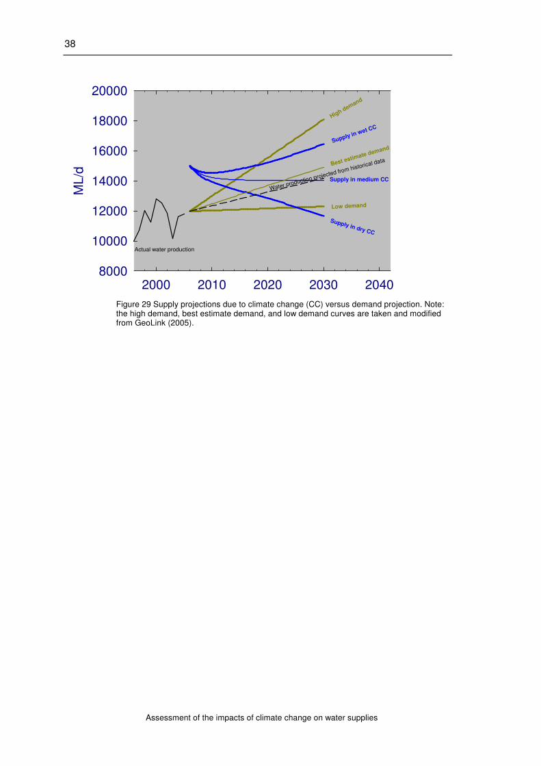
38
Assessment of the impacts of climate change on water supplies
2000 2010 2020 2030 2040
ML
/d
8000
10000
12000
14000
16000
18000
20000
High demand
Low demand
Supply in wet CC
Supply in dry CC
Best estimate demand
Supply in medium CC
Water production projected from historical data
Actual water production
Figure 29 Supply projections due to climate change (CC) versus demand projection. Note: the high demand, best estimate demand, and low demand curves are taken and modified from GeoLink (2005).
CONCLUSIONS 39
Assessment of the impacts of climate change on water supplies
5. CONCLUSIONS
This report has documented the framework and the results of the assessment of impacts of
climate change on Rous Water’s supplies. The quantitative assessments were conducted with
the aid of the Wilson River Integrated Quantity and Quality Model (IQQM). An alternative, i.e.
to scope changes in secure yields based on simple hydrological sensitivity models, has also
been made available.
In terms of risk of climate change the following are found:
• the increases in evaporation are virtually certain (i.e. > 99% likely). The lowest
and highest (5th and 95
th) changes range from about 2% to 4% in 2020, 4% to 12%
in 2020, and 10% to 26% in 2030.
• the chances of decreasing rainfall are relatively even with the chances of
increasing rainfall, particularly in the downstream tributary area. The lowest and
highest (5th and 95
th) changes in rainfall range from about 2% to -4% in 2010, 7%
to -11% in 2020, and 17% to -21% in 2030.
In terms of changes in the secure yield the results suggest that the decreases in secure yields are
highly likely in the future.
• The most likely (>50% probability) changes in secure yields are -3.4 %, -5.7%,
and -7.4% in 2010, 2020, and 2030 respectively.
• With regard to Lismore’s supply, the most likely (>50% probability) reduction is
about -0.5, -1.5%, and -2.5% in 2010, 2020, and 2030 respectively.
The results of the assessment suggest that:
• Given the best estimate demand and the driest supply scenario, the earliest time
for a new source is in 2018. Considering the best estimate demand and the
medium supply scenario, the medium time for a new source is in 2023.
• There is a two to seven year window of uncertainty regarding when the new
source has to be commissioned.
• Within this time, it is very important to monitor the demand and update the
assessment as to when to start building a new source. Ongoing monitoring of
rainfall pattern is also recommended.
40
Assessment of the impacts of climate change on water supplies
6. REFERENCES
Allen Consulting. 2005. Climate Change Risk and Vulnerability. Report to the Australian
Greenhouse Office, Department of the Environment and Heritage, Canberra,
Commonwealth of Australia, 159 pp.
BoM. 2006. Australian Bureau of Meteorology. www.bom.gov.au.
Chiew, F.H.S., Jones, R.N. and Boughton, W.R. 2005. Modelling hydrologic sensitivity to
climate conditions. Proceedings of the 29th Hydrology and Water Resources Symposium,
The Institution of Engineers Australia, Canberra. 9 pp.
CMPS&F. 1995. Rous Regional Water Supply Strategy Planning Study, Scheme Options, Final
Report. May 1995.
Department of Environment. 2004. Climate change, catchment runoff and risks to water supply
in the south-west of western Australia. Government of Western Australia, Department of
Environment.
DEH. 2005. Water conservation handbook for local government. Water Conservation
Partnership Project, South Australia. Department for Environment and Heritage.
DIPNR. 2004. Rous Water – Augmentation of Regional Water Supply Scheme, Hydrologic
modeling study using Wilsons River IQQM. Issue 3. NSW Department of Infrastructure,
Planning and Natural Resource
DLWC. 1998. Hydrology unit technical practice notes. NSW Department of Land an Water
Conservation.
Downing, T.E., Butterfield, R.E., Edmonds, B., Knox, J.W., Moss, S., Piper, B.S. and
Weatherhead, EK. 2003. CCDeW: Climate Change and Demand for Water. Defra.
EPICA. 2004. Eight glacial cycles from an Antarctic ice core. Nature, 429, 623-628.
Geolink. 2005. Dunoon Dam, Population and demand projections. Draft report, 19-08-2005.
Gleick, P. and Adams, A. 2000. Water: The potential consequences of climate variability and
change for the water resources of the United States. The report of the Water sector
assessment team of the national assessment of the potential consequences of climate
variability and change, for the U.S. Global Change Research Program.
Hennessy, K., Page, C., McInnes, K., Jones, R., Bathols, J., Collins, D. and Jones, D. 2004.
Climate change in New South Wales, Part 1: Past climate variability and projected
changes in average climate. Consultancy report for the New South Wales Greenhouse
Office.
Howe, C., Jones, R.N., Maheepala, S. and Rhodes, B. 2005. Melbourne water climate change
study, Implications of potential climate change for Melbourne’s water resources. A
collaborative project between Melbourne Water and CSIRO Urban Water and Climate
Impact Groups. Doc: CMIT-2005-106.
IPCC. 2001a. Summary for policymakers. In Houghton, J.T., Ding, Y., Griggs., D.J., Noguer,
M., Van Der Linden, P.J. and Xioaosu, D (eds) Climate Change 2001: The scientific
basis. Contribution of working group I to the third assessment report of the
Intergovernmental Panel on Climate Change, Cambridge University Press, Cambridge.
IPCC. 2001b. Climate Change 2001: Impacts, Adaptation and Vulnerability. McCarthy, J.,
Canziani, O., Leary, N., Dokken, D. and White, K (eds). Contribution of working group
II to the third assessment report of the Intergovernmental Panel on Climate Change,
World Meteorological Organisation and United Nations Environment Programme.
Cambridge University Press.
Jones, R.N. 2001. An environmental risk assessment/management framework for climate
change impact assessments. Natural Hazard, 23, 197-230.
Jones, R.N. and Page, C.M. 2001. Assessing the risk of climate change on the water resources
of the Macquarie River Catchment, in Ghassmi, F., Whetton, P. Little, R. and Littleboy,
M. (Eds). Integrating Models for Natural Resources Management across disciplines,

REFERENCES 41
Assessment of the impacts of climate change on water supplies
issues and scales (Part 2). Modsim 2001 International Congress on Modelling and
Simulation, Modelling and Simulation Society of Australia and New Zealand, Canberra,
673-678.
Jones, R.N. and McInnes, K.L. 2004. A scoping study on impact and adaptation strategies for
climate change in Victoria, A working paper produced as part of a three-year research
program on: Assessment of climate change, impacts and possible adaptation strategies
relevant to Victoria. April 2004.
Jones, R.N. and Preston, B.L. 2006. Adaptation actions for local government. A consultancy
report for SMEC Australia Pty Ltd., Draft January 2006.
Jones, R.N., Chiew, F.H.S., Boughton, W.B. and Zhang, L. 2006. Estimating the sensitivity of
mean annual runoff to climate change using selected hydrological models. Advances in
Water Resources, 29, 1419–1429.
Kirono, D.G.C., Page, C., Podger, G. and Jones, R. 2006. Assessment of the impacts of climate
change on water supplies. Mid-term report prepared for Rous Water New South Wales
Department of Commerce. June 2006.
Montgomery Watson. 2000. Improving water use efficiency in Queensland’s Urban
Communities, Quensland Department of Natural resources. Final report.
Morton, FI. 1983. Operational estimates of areal evapotranspiration and their significance to
the science and practice of hydrology. Journal of Hydrology, 66, 1-76.
Nakicenovic, N. (ed). 2000. Special Report on Emissions Scenarios. A Special Report of
Working Group III of the Intergovernmental Panel on Climate Change,
Intergovernmental Panel on Climate Change.
Our Water Our Future. 2005. Draft for community comment secure water strategy central
region.
Page, C.M., and Jones, R.N. 2001. OzClim: the development of a climate scenario generator for
Australia. In: MODSIM 2001: International Congress on Modelling and Simulation:
proceedings, Australian National University, F. Ghassemi, and others (editors).
Canberra, ACT: Modelling and Simulation Society of Australia and New Zealand. p.
667-671.
Pittock, A.B. and Jones, R.N. 2000. Adaptation to what, and why? Environmental Monitoring
and Assessment, 61, 9-35.
Pittock, A.B. 2003. Climate change: an Australian guide to the science and potential impacts.
The Australian Greenhouse Office, Canberra.
Rous Water. 1995. Rous regional water supply strategy planning study. Scheme options. Final
Report May 1995.
Rous Water. 2002. Ballina heights dual reticulation feasibility study. Rous Water Regional
Authority. Final report March 2002.
Rous Water. 2004. Demand management plan, 2004-2009. Rous Water Regional Water
Supply, Adopted Council Meeting March 2004.
Rous Water. 2006. A Presentation about Rous Water Regional Supply.
www.scu.edu.au/schools/esm/dds. Downloaded in 02 June 2006.
Vivès, B. and Jones, R.N. 2005. Detection of abrupt changes in Australian decadal rainfall
(1890-1989). CSIRO Atmospheric Research Technical Paper 73.
Water Proofing Adelaide. 2004. Water proofing Adelaide, Exploring the issues – a discussion
paper. Government of South Australia, Action Salinity Australia, Water Care.
WMO. 2003. WMO statement on the status of the global climate in 2003. World
Meteorological Organisation. http://www.mwo.ch/web/Press/index.html

42
Assessment of the impacts of climate change on water supplies
APPENDIX 43
Assessment of the impacts of climate change on water supplies
APPENDIX
The iterative solution that successively modifies and runs IQQM until the demand is met such
the 5/10/20 rule is just met is as follows:
1. Set initial upper and lower search limits (5,700 and 18,500 ML/a)
2. Determine current secure yield by taking average of the upper and lower search limit
(initially 12,100 ML/a)
3. Create a new pattern file that proportionally adjusts Ballina demand for the current
secure yield
4. Create an IQQM macro language file that:
• Points to the new pattern file
• Points to the appropriate climate scenario rainfall, evaporation and flow time series
database
• Adjusts the 10 other demand centres based on the current secure yield
• Runs the FX94D scenario model from 1/1/1900 to 31/12/2001
• Outputs the combined storage volume of Rocky Ck and Emigrant Ck dams to a CSV
file
• Outputs the daily volume extracted at the Lismore source
5. Runs IQQM via the macro language file
6. Reads the combined storage volume CSV file
7. Sums the number of days of restriction
8. Sums the number of years with restrictions based on a July water year
9. Reads the Lismore source file and determines the average annual extraction volume at
Lismore source
10. Checks if the number of days of restriction are <= 1862 and number of years of
restriction are <= 10
11. If either is not met and the number of iterations is less than 7 makes the upper secure
yield equal to the current yield and repeats to step 2
12. If it is met continues to step 9
13. Creates a new macro language file similar to step 4 except
14. Runs FX94Dr scenario model that contains Rocky Ck Dam and Emigrant Ck dam at
55% capacity and permanent restrictions
15. Only outputs Rocky Ck dam volume to a CSV file
16. Runs IQQM via the macro language file
17. Reads the Rocky Ck storage volume
18. If it reaches 150 ML makes the upper secure yield equal to the current yield
19. If it does not reach 150 ML makes the lower secure yield equal to the current yield
20. If the number of iterations are less than 7 repeats to step 2
21. After 7 iterations the lower secure yield value represents the secure yield to an accuracy
of 0.1 ML/a
Copyright © 2022 FDOKUMEN