Climate change impacts on agricultural vegetation in sub ...
171
Universität Potsdam, Institut für Erd- und Umweltwissenschaften und Potsdam Institut für Klimafolgenforschung Climate Change Impacts on Agricultural Vegetation in Sub-Saharan Africa Dissertation zur Erlangung des akademischen Grades "doctor rerum naturalium" (Dr. rer. nat.) in der Wissenschaftsdisziplin Geoökologie eingereicht an der Mathematisch-Naturwissenschaftlichen Fakultät der Universität Potsdam von Katharina Waha Potsdam, den 18.Juni 2012
-
Upload
khangminh22 -
Category
Documents
-
view
2 -
download
0
Transcript of Climate change impacts on agricultural vegetation in sub ...

Universität Potsdam, Institut für Erd- und Umweltwissenschaften
und Potsdam Institut für Klimafolgenforschung
Climate Change Impacts on Agricultural Vegetation
in Sub-Saharan Africa
Dissertation
zur Erlangung des akademischen Grades
"doctor rerum naturalium"
(Dr. rer. nat.)
in der Wissenschaftsdisziplin Geoökologie
eingereicht an der
Mathematisch-Naturwissenschaftlichen Fakultät
der Universität Potsdam
von
Katharina Waha
Potsdam, den 18.Juni 2012

Published online at the Institutional Repository of the University of Potsdam: URL http://opus.kobv.de/ubp/volltexte/2013/6471/ URN urn:nbn:de:kobv:517-opus-64717 http://nbn-resolving.de/urn:nbn:de:kobv:517-opus-64717

Danksagung
Ich möchte mich bei den Menschen bedanken die mich während der Promotionszeit
unterstützt haben und denen ich zu verdanken habe, dass ich nie den Spaß an
meiner Forschungsarbeit verloren habe.
Mein herzlicher Dank gilt Christoph Müller, Hermann Lotze-Campen und Wolfgang
Cramer die mich fortwährend und vorbehaltlos fachlich und persönlich unterstützt
haben und mir außerdem wichtige Reisen zu Konferenzen und Workshops
ermöglicht haben. Danke für euer Vertrauen und das ihr mir den so wichtigen Raum
gelassen habt eigene Forschungsideen zu entwickeln und umzusetzen.
Ich danke allen LPJ/LPJmL Entwicklern und vor allem Christoph Müller, Jens Heinke,
Sibyll Schaphoff und Werner von Bloh für ihr ständiges Bemühen das Modell zu
verbessern, den Modellcode zu pflegen und für ihre Hilfestellungen und Hinweise bei
allen Programmier- und technischen Fragen. Allen Mitgliedern der landuse Gruppe
am PIK danke ich für die freundschaftliche und hilfsbereite Begleitung meiner
Promotionszeit. Ein besseres Arbeitsumfeld kann man sich nicht wünschen. Jeder
von euch hatte immer ein offenes Ohr für meine Fragen und Probleme. Jan, danke,
dass du mich an guten und nicht so guten Arbeitstagen begleitet hast, für deine
großartigen Einfälle und dafür, dass du immer Zeit und Muße hattest meine Ideen zu
hinterfragen und zu diskutieren.
I am grateful to Alberte Bondeau, Christoph Müller, Lenny van Bussel and Susanne
Rolinski for there inspiring ideas on our joint work and for being very encouraging and
friendly colleagues. Thanks, Alberte and Christoph for accompanying my first steps
with LPJmL and for being such motivated and lovely colleagues and supervisors.
Auch wenn sie meinen es wäre nicht nötig, danke ich meinen Eltern für ihre
Unterstützung und Liebe, sie sind meine Vorbilder. Stephan, ich danke dir für so
vieles, ich kann es hier nicht alles aufzählen. Du hast mich die ganze Zeit begleitet
und ich hoffe es wird immer so sein.
i

ii

Table of contents
Danksagung................................................................................................................i
List of figures...........................................................................................................vii
List of tables .............................................................................................................xi
1. Introduction ........................................................................................................1
1.1. Background...................................................................................................1
Agriculture in sub-Saharan Africa.........................................................................1
Quantifying climate change impacts on agricultural vegetation............................6
1.2. Objectives and outline.................................................................................11
2. Climate-driven simulation of global crop sowing dates ...............................15
2.1. Introduction .................................................................................................16
2.2. Materials and Methods................................................................................18
Input climate data...............................................................................................18
Deterministic simulation of sowing dates ...........................................................18
Determination of seasonality types ....................................................................19
Determination of the start of the growing period.................................................21
Procedure of validating the methodology ...........................................................24
2.3. Results ........................................................................................................26
Seasonality types ...............................................................................................26
Comparison of observed and simulated sowing dates .......................................27
2.4. Discussion...................................................................................................31
Pulses and groundnuts in multiple cropping systems.........................................32
Maize in multiple cropping systems in Southeast Asia.......................................33
Wheat and rapeseed in temperate regions ........................................................33
Cassava in multiple cropping systems ...............................................................34
2.5. Conclusions ................................................................................................36
2.6. Acknowledgements .....................................................................................37
2.7. Authors´ contribution ...................................................................................37
iii

3. Adaptation to Climate Change through the Choice of Cropping System and Sowing date in Sub-Saharan Africa.......................................................................39
3.1. Introduction .................................................................................................41
3.2. Materials and Methods................................................................................44
Input data for current and future climate ............................................................44
Household survey ..............................................................................................46
Identification of sequential cropping systems.....................................................46
Management scenarios for adaptation ...............................................................48
Dynamic global vegetation model for managed land LPJmL..............................49
Modelling the spatial variation of PHUsin and PHUseq .........................................54
Theoretical potential of sequential cropping systems.........................................54
3.3. Results ........................................................................................................55
Sequential cropping systems in sub-Saharan Africa ..........................................55
Growing periods and PHUs of different crop cultivars........................................57
Changes in crop yields.......................................................................................59
Potential of sequential cropping systems in sub-Saharan Africa........................62
3.4. Discussion...................................................................................................64
Changes in crop yield.........................................................................................64
Limitations of the modeling approach.................................................................67
Uncertainties from the household survey ...........................................................68
Farmers’ adaptation options...............................................................................69
3.5. Summary and Conclusions .........................................................................71
3.6. Acknowledgements .....................................................................................72
3.7. Authors´ contribution ...................................................................................72
4. Separating the effects of temperature and precipitation change on maize yields in sub-Saharan Africa ..................................................................................73
4.1. Introduction .................................................................................................75
4.2. Materials and Methods................................................................................77
Climate data .......................................................................................................77
Climate experiments ..........................................................................................78
Modelling the impact on agricultural vegetation .................................................80
4.3. Results ........................................................................................................82
Changes in temperature, wet season length and precipitation amount..............83
Impacts on agricultural vegetation in sub-Saharan Africa ..................................84
4.4. Discussion...................................................................................................86
iv

Aggregating and understanding crop yield changes ..........................................86
Uncertainty in GCM projections of precipitation .................................................90
Limitations of modeling stress on crop growth and development .......................91
4.5. Summary and conclusions ..........................................................................92
4.6. Acknowledgements .....................................................................................93
4.7. Authors´ contribution ...................................................................................93
5. General Conclusions .......................................................................................95
5.1. Key results and conclusions........................................................................95
5.2. Future research priorities ............................................................................98
Up-scaling multiple cropping data to global scale ..............................................98
Analyse the effect of abiotic stress factors on crops ..........................................99
Bridging the gap between model scales...........................................................100
Summary................................................................................................................103
Appendices ............................................................................................................105
A Analysis of sowing date patterns of eleven crops .....................................105
B Sensitivity analysis of crop yield on sowing date.......................................117
Methodology.....................................................................................................117
Results and Discussion....................................................................................117
C Water stress affecting root biomass..........................................................119
D Comparison of the start of the growing season to satellite data................120
E Model’s ability to simulate national crop yields in sub-Saharan Africa ......121
F Detailed list of simulated crop yields per location......................................125
G Global circulation models used in this study .............................................130
H Method of generating stylized precipitation scenarios...............................131
Identifying the largest change in wet season characteristics............................131
Overestimation of precipitation changes ..........................................................132
I Method for calculating crop yield and crop yield changes .........................135
References.............................................................................................................137
v

vi

List of figures
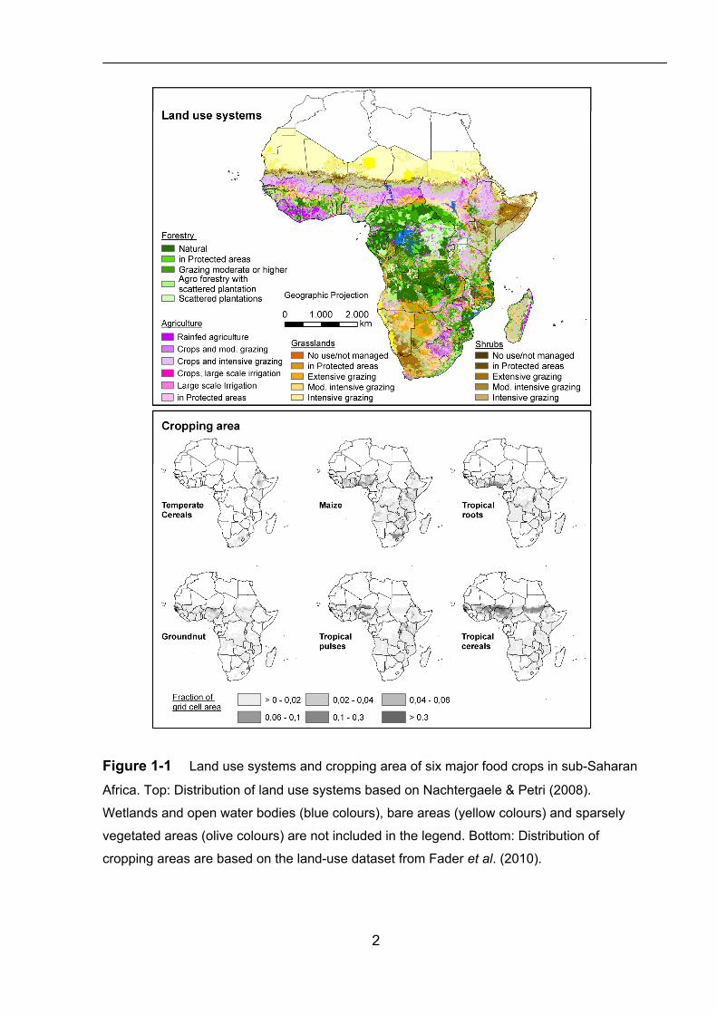
Figure 1-1 Land use systems and cropping area of six major food crops in sub-
Saharan Africa. ................................................................................................................2
Figure 1-2 Mean change in crop yields, population and food self-sufficiency in
ten world regions from 1996-2005 to 2046-2055 in 30 climate change scenarios............5
Figure 1-3 Graphical abstract of thematic focus, scale of study region and crops
studied in the main chapters...........................................................................................13
Figure 2-1 Procedure to determine seasonality type and sowing date. ..................19
Figure 2-2 Global distribution of seasonality types. ...............................................27
Figure 2-3 Annual variations in temperature (above) and precipitation (below) for
five locations. ..............................................................................................................28
Figure 2-4 Cumulative percent of grid cells (or crop area in a grid cell) with
certain differences between observed and simulated sowing date.................................29
Figure 3-1 Change in annual mean temperature and annual mean precipitation
from 1971-2000 to 2070-2099 projected from three GCMs under the SRES A2............45
Figure 3-2 Scheme of possible timing and length of growing periods of crops in
single cropping systems (A-C) and sequential cropping systems (D-G) according to
the definition used in this study. .....................................................................................47
Figure 3-3 Most frequently applied rainfed sequential cropping systems in sub-
Saharan Africa. ..............................................................................................................56
Figure 3-4 Deviations in days between simulated and observed length of
growing period in 2002/03 in single cropping systems ...................................................59
Figure 3-5 Mean crop yields [Mcal/ha] per region in 1971-2000 and in 2070-
2099 if TS/TSco (the traditional sequence cropping systems), SC/SCco (only the first
crop of the traditional sequential cropping systems), or HS/HSco (the highest-yielding
sequential cropping systems) are applied ......................................................................60
vii

Figure 3-6 Mean crop yield changes (%) in 2070-2099 compared to 1971-2000
with corresponding standard deviations (%) in six single cropping systems (upper
panel) and 13 sequential cropping systems (lower panel)..............................................63
Figure 4-1 Precipitation in the wet season (mm), length of the wet season
(days) and annual mean temperature (°C) in the 1995s as calculated from daily
precipitation and monthly temperatures. ........................................................................79
Figure 4-2 Graphical abstract of data, methods and expected results in this
study. ..............................................................................................................82
Figure 4-3 Change in important agroclimatic variables according to GCM
projections in the 2060s (top) and 2085s (bottom) compared to the 1995s (from left to
right): wet season precipitation, wet season length and annual mean temperature. ......84
Figure 4-4 Changes in rainfed maize yield calculated with LPJmL in the 2060s
(top) and 2085s (bottom), due to (from left to right) increasing annual mean
temperature (Ct), shortened wet season (Cl), reduced wet season precipitation (Cp),
and the combined effect from all three (CpClCt). ...........................................................86
Figure 4-5 Distribution and characteristics of four groups resulting from
hierarchical cluster analyses of yield changes in the 2060s ...........................................87
Figure 4-6 Crop yield changes in the 2060s from the combined (CpClCt) and
separated effects of changing temperature (Ct) and wet seasons (Cp, Cl) in groups
shown in Figure 4-5........................................................................................................89
Figure 5-1 Achievable increases in global crop production (%) through different
water management and cropping system management strategies under climate
change in the 2055s as compared to the current state...................................................97
Figure A-1 Analysis of sowing date patterns of wheat. .........................................106
Figure A-2 Analysis of sowing date patterns of rice..................................................107
Figure A-3 Analysis of sowing date patterns of maize. .............................................108
Figure A-4 Analysis of sowing date patterns of millet. ..............................................109
viii

Figure A-5 Analysis of sowing date patterns of pulses. ............................................110
Figure A-6 Analysis of sowing date patterns of sugar beet.......................................111
Figure A-7 Analysis of sowing date patterns of cassava. .........................................112
Figure A-8 Analysis of sowing date patterns of sunflower. .......................................113
Figure A-9 Analysis of sowing date patterns of soybean. .........................................114
Figure A-10 Analysis of sowing date patterns of groundnut. ...................................115
Figure A-11 Analysis of sowing date patterns of rapeseed. ....................................116
Figure B-1 Sensitivity of maize yield to sowing dates for five locations. ...................118
Figure C-1 Biomass fraction allocated to the roots as simulated in LPJmL ..............119
Figure D-1 Comparison of A: simulated and B: observed start of the growing
season (in weeks). .......................................................................................................120
Figure E-1 Comparison of LPJmL and FAO cassava yields. ....................................122
Figure E-2 Comparison of LPJmL and FAO cowpea yields......................................122
Figure E-3 Comparison of LPJmL and FAO groundnut yields. .................................123
Figure E-4 Comparison of LPJmL and FAO maize yields.........................................123
Figure E-5 Comparison of LPJmL and FAO rice yields. ...........................................124
Figure E-6 Comparison of LPJmL and FAO wheat yields. .......................................124
Figure H-1 Daily precipitation changes in the 2060s for an example cell..................132
Figure H-1 Distribution function (top) and cumulative distribution function (bottom)
of the length of the wet season (left) and the precipitation amount in the wet season
(right) in the baseline climate calculated from the WATCH Forcing Data (WFD) and
from nine GCMs. ..........................................................................................................134
ix

x

List of tables
Table 1-1 Large-scale crop models.............................................................................8
Table 2-1 Crop-specific temperature thresholds for sowing. .....................................23
Table 2-2 Indices of agreement between simulated sowing dates and observed
sowing dates. .................................................................................................................31
Table 3-1 Definition of terms used in this study. .......................................................42
Table 3-2 Crop-specific parameters for estimating PHUs in single and sequential
cropping systems and calculating fresh matter crop yields in kcal/ha. ...........................53
Table 3-3 Highest-yielding rainfed sequential cropping systems in the period
1971-2000 in 63 districts in seven sub-Saharan Africa countries depending on the
location within the country. .............................................................................................57
Table 3-4 Time from sowing to harvest in months for different crop cultivars found
in the household survey and in literature........................................................................58
Table 3-5 Mean crop yields and crop yield changes per GCM and management
scenario in 63 districts of seven sub-Saharan Africa countries in the period 2070-
2099 compared to the period 1971-2000 in six management scenarios. .......................61
Table 3-6 Change in climate and length of the crops´ growing period in the period
2070-2099 compared to the period 1971-2000 in six management scenarios using
climate projections from three GCMs. ............................................................................65
Table 3-7 Comparison of simulated crop yields from literature and this study. .........66
Table 5-1 Abiotic stress factors considered in large-scale models simulating
agricultural vegetation. ...................................................................................................99
xi

xii
Table F-1 Overview of mean crop yields and crop yield changes per country and
management scenario in 2070-2099 compared to 1971-2000 averaged over three
GCMs. ................................................................................................................125
Table G-1 Global circulation models used in this study ...........................................130

1. Introduction
This chapter describes the importance of agriculture in sub-Saharan Africa and the
challenges the agricultural sector faces today and is likely to face in future. One of
these challenges – climate change and its impacts on agriculture is defined as the
core subject of this thesis and I later narrow this to the main objectives of this thesis
and explain the methods applied to achieve them.
1.1. BACKGROUND
Agriculture in sub-Saharan Africa
Agricultural areas cover a large part of the Earth’s land area; for this reason, changes
in agricultural systems cause important feedbacks to the atmosphere, soils,
hydrological systems and more parts of the Earth system. For humans, agriculture is
one of the most important land use activities, as it provides food, energy, fibre and
other land-based products. Agriculture plays a key role in many countries, but in
developing countries especially a sustainable agricultural sector ensures food and
livelihood for many people and reduces poverty. In sub-Saharan Africa agriculture is
also of major importance for humans which can be seen in the following indicators:
- Large parts of the land area are used as agricultural area. In 2010, 43 %
(World: 38 %) of the land area was managed by humans as land under
temporary and permanent crops, pasture and gardens, grazing land and land
for agro-forestry (FAO, 2011). Approximately 8 % of the land area in tropical
Africa is used for agricultural crops only (Ramankutty et al., 2008) and
Western Africa has the highest share of cropland in total land of 14 %
(Fischer et al., 2011). The most important agricultural areas lie in a band
stretching from west to east between 5° N and 15° N and in a band running
parallel to the Indian Ocean coastline from Ethiopia to South Africa (Figure 1-
1).
1
2
Figure 1-1 Land use systems and cropping area of six major food crops in sub-Saharan
Africa. Top: Distribution of land use systems based on Nachtergaele & Petri (2008).
Wetlands and open water bodies (blue colours), bare areas (yellow colours) and sparsely
vegetated areas (olive colours) are not included in the legend. Bottom: Distribution of
cropping areas are based on the land-use dataset from Fader et al. (2010).

Introduction
3
- Economy depends on agriculture. 13 % (World 3 %) of the regions gross
domestic product is produced by agriculture (World Bank, 2012), with many
countries generating one third or more of their gross domestic product by
agriculture (Central African Republic, Democratic Republic of Congo,
Ethiopia, Ghana, Malawi, Mozambique, Rwanda, Sierra Leone). The majority
of African countries is classified as “low-income food-deficit countries”, which
indicates their low per capita gross national income and their dependency on
food imports, making them vulnerable to food crises (FAO, 2008; FAO,
2012).
- People are reliant on the agricultural sector for their livelihood. 55 % (World
38 %) of the population depends on agriculture, hunting, fishing or forestry,
including not only the economically active persons but also their non-working
family members (FAO, 2011a).
However, agriculture in sub-Saharan Africa is rather unproductive compared to other
world regions because of limited technical knowledge and finances which is required
to increase production by the use of e.g. irrigation, fertilizer, machinery or soil-
conservation measures, limited storage capacity for the produced agricultural goods
and limited access to consumer markets (Godfray et al., 2010). Almost two thirds of
the cropping area is prepared by hand and the consumption of mineral fertilizer of
5 kg/ha in 1997-1999 is very low compared to East and South Asia with 194 kg/ha
and 103 kg/ha respectively (FAO, 2003). Therefore, yields of the most important food
crops in sub-Saharan Africa in the year 2000 only reached between 33 % (maize)
and 88 % (cassava) of yields that would be achieved with global average
management intensity (Dietrich et al., 2012). Compared to the potentially achievable
yield, the actually achieved crop yields are even lower by a factor of four (Fischer et
al., 2011). The unstable political and economical situation, security conflicts and
unsecure land rights together with a high vulnerability to fluctuating world market
prizes increase the pressure on the agricultural sector even more.
At the same time a doubling of the African population from 2000 to 2050 is expected
(Figure 1-2), which together with shifting diets and incomes will cause large growth
rates for the demand for food and livestock products of 2.8 % per year until 2030 and
2.0 % per year until 2050 thereafter (FAO, 2006). In the past, production of

Introduction
4
agricultural goods in sub-Saharan Africa was enhanced by expanding arable land,
improving crop yields and increasing cropping intensity, i.e. expanding multiple
cropping areas and reducing fallow periods. All three sources of growth contributed in
equal parts and historical production growth between 1969-99 was 2.3 % per year
(FAO, 2003). It is expected for 2030 that about 60 % of production growth will
originate from increasing crop yields only (FAO, 2003). Large annual yield increases
of 2.0 % per year until 2055 (World 1 % per year) are required to fulfill the demand for
agricultural goods even in a business-as-usual scenario with increasing population,
continued cropland expansion at historical rates and further globalization and trade
liberalization. When taking increasing demand for bioenergy and extended efforts to
protect intact and frontier forest into account as additional pressures, productivity is
required to increase even more by 2.1 % p.a. and 2.3 % p.a., respectively (Lotze-
Campen et al., 2009).
In this context, climate change poses an additional risk for agriculture in sub-Saharan
Africa. Warming during the 21st century is very likely to be larger than the global
annual mean warming in Africa in all seasons and in all countries (Christensen et al.,
2007) making the continent one of the most susceptible world regions. Temperature
is projected to increase by up to 3 °C until the end of the 21st century for the emission
scenario A1b in equatorial and coastal areas and by up to 4 °C in the western Sahara
compared to the end of the 20th century, and additionally a robust drying of the
northern Sahara, the African west coast and Southern Africa is projected from most
of the general circulation models (GCMs) (Christensen et al., 2007) which will
influence the growing conditions of agricultural crops.
Agricultural production in sub-Saharan Africa is expected to be severely influenced
by climate change depending on the region, crop type, farming system, climate
change scenario and method for assessing these effects. Mean country yields from
eleven major food crops simulated with the dynamic global vegetation model LPJmL
for five GCMs, three emission scenarios and two CO2 fertilization scenarios are
expected to change by -12.9 % to +17.3 % by 2050 (Figure 1-2). Food self-
sufficiency will decrease most strongly in sub-Saharan Africa and the MENA region
(Middle East and North Africa) compared to other world regions even if crop yields in
some locations increase due to enhanced growing conditions. This unstable food
situation increases the risk for regional food crises, and might also weaken the social

Introduction
5
and political stability of countries (Scheffran & Battaglini, 2011). A database on social
conflicts in Africa lists over 7300 social conflict events between 1990 to 2010,
including 324 demonstrations or violent riots because of food, water or subsistence
issues (Hendrix & Salehyan, 2012).
Figure 1-2 Mean change in crop yields, population and food self-sufficiency in ten world
regions from 1996-2005 to 2046-2055 in 30 climate change scenarios (Müller et al., 2009).
Food self-sufficiency is calculated as the ratio of food production to food demand. Whiskers
indicate the range of impacts. Population growth rates were taken from Nakicenovic & Swart
(2000) for three emission scenarios.

Introduction
6
Quantifying climate change impacts on agricultural vegetation
In the context of food supply and food security globally and in developing countries
researchers aim at understanding and projecting climate change impacts on
agricultural crops using various approaches. Among the first studies was the global
food supply study from Rosenzweig & Parry (1994) which was later extended in the
studies from Parry et al. (2004) and Parry et al. (2005). They use yield transfer
functions derived from crop model simulations on the effects of climate change,
increasing atmospheric CO2 concentrations and adaptation options on crop yields.
These results strongly depend on the crop model used to simulate crop responses to
changing climate in a region. Rosenzweig & Parry (1994) extrapolated crop
responses from 18 crop models and only 112 sites to national levels which are not
representative for all regions, e.g. for Africa where crop model results for only one
site in Zimbabwe was included. Another uncertainty in these studies arises from
merging results from different crop models which differ in model parameters, model
structure and settings. Each of them has to be calibrated to local soil, climate and
agronomic conditions and cannot be extrapolated to other locations easily.
In the agro-ecological zones approach attainable crop yields are calculated
depending on the growing season length, temperature, precipitation, soils and
terrains (Fischer et al., 2002b) with a simple crop model using empirical relationships
without considering the underlying process (Tubiello & Ewert, 2002). Attainable yields
will change if climatic conditions, and in turn the distribution of agro-ecological zones
change, therefore the impact of slight climate change leading to a shift in zones might
be overestimated considerably (Mendelson & Dinar, 1999). Also this approach
projects the potential distribution of crops and crop yields rather than the actual
situation and results need validation (Fischer et al., 2002b).
A similar approach to the yield transfer functions is to develop a statistical model from
historical crop yields and monthly temperature and precipitation data for the same
period which was done for sub-Saharan Africa in Lobell et al. (2008) and in
Schlenker & Lobell (2010). Here the crop response is not based on crop models but
on crop yields measured in the field or estimated from farmers or agronomist which
are also subject to various uncertainties (Fermont & Benson, 2011). Another
deficiency arise from combining crop yield data with gridded climate data which might

Introduction
7
be of low quality in regions with only few weather stations. The most important
limitation of statistical models is that they cannot be extrapolated to project crop
yields in climatic conditions different from the historic climate (Lobell et al., 2008).
Lobell et al. (2008) therefore recommend applying statistical models only for studies
until 2030 and rely on process-based crop models in studies for the end of the 21st
century.
Process-based crop models simulate key plant processes like photosynthesis, plant
phenology, carbon assimilation and allocation to plant organs and the dynamics of
carbon and water from climate and soil data. They are therefore able to capture the
dynamics of crop responses to climate change (Tubiello & Ewert, 2002). The study
region stretches over 8000 km from north to south and over 7400 km from west to
east so they need to be applicable at a large scale and for different environments. To
my knowledge currently seven models designed to study the effect of climate change
on agricultural vegetation on a large scale are published: DSSAT-CSM, ORCHIDEE-
STICS, DayCent, LPJmL, GEPIC, ORCH-mil, and Pegasus (ordered ascending by
the year of their first release). They differ in their model components and in the crops
and management options included but all seven are intended to simulate crop
growth, development and yield in a process-based way from soil and climate input
data on a large scale. Table 1-1 shows the key reference describing each model, the
crops included and the regions each model was applied for.
DSSAT-CSM, based on the decision support system DSSAT which was first released
in 1989, is a combination of 16 individual crop and grass models from the CERES
and CROPGRO model families. Researchers have frequently applied the DSSAT-
CSM crop models in local studies on the effect of various management strategies on
crop yields, and also in regional climate change impact studies (Jones et al., 2003).
DayCent, a daily time step model of the CENTURY biogeochemical model (Parton et
al., 1994), is an agro-ecosystem model which was adjusted at the Netherlands
Environmental Assessment Agency to simulate the effects of climate, soil and crop
management on crop yields of wheat, rice, maize and soybean at the global scale
(Stehfest et al., 2007).

Introduction
8
Table 1-1 Large-scale crop models.
Model Key reference Scale / Regions Crops
DSSAT-CSM Jones et al. (2003) Various single countries and world regions
chickpea, cowpea, dry bean, faba bean, maize, millet, peanut, potato, rice, sorghum, soybean, tomato, velvet bean, wheat
ORCHIDEE-STICS
Gervois et al. (2004) Europe, USA maize, soybean, winter wheat
DayCent Stehfest et al. (2007) Global maize, rice, soybean, wheat
LPJmL Bondeau et al. (2007) Global cassava, groundnut, maize, millet, pulses, rapeseed, rice, soybean, sugar beet, sunflower, wheat
GEPIC Liu et al. (2007) Global, China, sub-Saharan Africa
cassava, maize, millet, rice, sorghum, wheat
ORCH-mil Berg et al. (2010) West Africa millet
Pegasus Deryng et al. (2011) Global maize, soybean, wheat
GEPIC, which is a GIS based model of the EPIC model designed at the Swiss
Federal Institute of Aquatic Science and Technology (Liu et al., 2007), was applied
for sub-Saharan Africa, China and on the global scale. The original EPIC model
(Jones et al., 1991; Williams et al., 1989) provides a lot of important soil or crop
parameters which are adopted from many other global crop models. Pegasus,
recently developed at the Tyndall Centre for Climate Change Research and the
McGill University, simulates maize, soybean and spring wheat growth, fertilizer
application, irrigation and dynamic planting dates (Deryng et al., 2011).
The ORCHIDEE-STICS and ORCH-mil models as well as the LPJmL model are
based on the dynamic global vegetation models ORCHIDEE and LPJ-DGVM
respectively which were further improved by including agricultural crops. ORCHIDEE-
STICS was developed in 2004 at the Laboratoire des Sciences du Climat et de
l’Environnement with the aim of including croplands (Gervois et al., 2004). As the
model was tested and validated only for winter wheat, maize and soybean but not for
tropical crops, ORCH-mil was developed at the Institut Pierre Simon Laplace from the

Introduction
9
original ORCHIDEE model by including tropical C4 crops. ORCH-mil is therefore able
to simulate millet growth and yield in West Africa (Berg et al., 2010).
LPJmL (Bondeau et al., 2007) is an improved version of the LPJ-DGVM (Sitch et al.,
2003), developed at Lund in Sweden and Potsdam and Jena in Germany, as it now
also includes agricultural crops. It is the most suitable tool for this study because of
its ability to simulate crop yields for the major agricultural crops (Table 1-1) under
current and future climates with a manageable amount of model parameters and low
input requirements compared to e.g. DSSAT-CSM or GEPIC. The model’s source
code is written in C, which provides the possibility to include new functionalities. The
model furthermore is already prepared to run on a high performance cluster
computer, saving a lot of computation time. This allows obtaining simulation results
for a large range of climate scenarios, emission scenarios, and model setups on a
high spatial and temporal resolution.
LPJmL is able to simulate crop yields of eleven crop types in single-cropping
systems; these are already validated for maize and wheat in temperate regions
(Bondeau et al., 2007; Fader et al., 2010). A global land-use dataset and a method
for representing agricultural management intensity was described recently in Fader et
al. (2010), and evapotranspiration and crop water consumption were tested and
validated against observational data (Gerten et al., 2004; Rost et al., 2008). The
eleven crop types included in the model cover nearly 70 % of the area harvested and
48 % of the total crop production in sub-Saharan Africa. For studying climate change
impacts in sub-Saharan Africa it was necessary to adapt the model to growing
conditions in tropical ecosystems, which is done in this thesis for crop phenology and
for cropping systems. Before, crops´ sowing dates were not represented well or even
missing in the tropics. Therefore an improved rule for farmers´ planting decisions was
developed in order to time sowing dates to the beginning of the rainy season.
Furthermore, tropical cropping systems are much more complex than single cropping
systems usually found in the temperate zone and therefore multiple cropping systems
were implemented into LPJmL. For this purpose, the parameterization of a crop’s
growing period has to be changed to allow the simulation of short and long growing
crop varieties depending on the length of the growing season and the cropping
system. The model is further described in the “Materials and Methods” sections of

Introduction
10
each chapter highlighting the relevant model functionalities and model settings for
each study.
Only few climate change impact studies with a focus on sub-Saharan Africa using a
process-based crop model were conducted and described in the literature: for maize
with CERES-maize (Jones & Thornton, 2003), for maize and beans with DSSAT
(Thornton et al., 2011), for six major crops with GEPIC (Liu et al., 2008) and recently
for maize with GEPIC (Folberth et al., 2012). Additionally impact studies for individual
countries or regions and crops can be found in literature for e.g. Cameroon with
CropSyst (Laux et al., 2010; Tingem & Rivington, 2009), East Africa with DSSAT
(Thornton et al., 2009; Thornton et al., 2010), Mali with EPIC (Butt et al., 2005),
Nigeria with EPIC (Adejuwon, 2006), Ghana with GEMS (Tan et al., 2010) and South
Africa with CERES-maize (Walker & Schulze, 2008). However, all of the above-
mentioned studies for sub-Saharan Africa and most of the regional studies omit
including and discussing management strategies for adaptation and their effect on
crop yield changes. The studies from Tingem & Rivington (2009), Laux et al. (2010)
and Thornton et al. (2010) are an exception considering adapted sowing dates,
adapted crop cultivars and shifts in farming systems but only for Cameroon and East
Africa. The most comprehensive study from Butt et al. (2005) for Ghana simulates a
wide range of biophysical adaptation, economic adaptation and policy based
adaptation options like e.g. cropping patterns, the choice of improved and heat-
resistant varieties and expansion of cropland. Theses studies are promising first
regional assessments of the potentials of different adaptation options but lack in
being widely applicable for the whole continent.

Introduction
11
1.2. OBJECTIVES AND OUTLINE
This thesis is divided into three main parts; each of them intended to achieve specific
goals but also following the findings from the preceding chapter in order to contribute
answering the central research questions:
1. What are the impacts of climate change on agricultural crops in sub-Saharan
Africa in the middle and end of the 21st century?
2. What is the potential of adaptation options for reducing negative climate
change impacts in sub-Saharan Africa?
3. What are the determining factors for negative climate change impacts in sub-
Saharan Africa?
Chapter 2: This first part sets the stage for quantifying climate change impacts on
agricultural crops using a global crop model. It addresses the problem of simulating
crop sowing dates on a global scale and of understanding the importance of climate
in determining sowing dates. The global crop model so far is not able to simulate any
sowing date for many important crops in the tropics and in other world regions they
are incorrect or not validated to cropping calendars. This is a main shortcoming of the
model as the timing of sowing largely determines crop growth and development, the
occurrence of water stress in different development stages and final crop yields.
Existing approaches either prescribe sowing dates (e.g. in GEPIC) or optimize them
to reach highest possible crop yields (e.g. in DayCent). While the first approach
cannot be applied in a climate change study as sowing dates will not be adapted to
new climatic conditions, the optimization approach is limited by uncertainties in the
model used to simulate crop yield. I develop an improved, simple rule for determining
the timing of sowing from monthly climatology based on the existing approach
described in Bondeau et al. (2007). Farmers in the tropics base their timing of sowing
on the onset of the rainy season and this important management strategy needs to
be considered in climate change impact studies as well. I also validate the simulated
sowing dates from eleven crops by comparing them to sowing dates from a global
crop calendar.

Introduction
12
Chapter 3: From the results of chapter 2 I realized that substantial deviations in
sowing dates occur in tropical regions and regions with high-land use intensity as
only single cropping systems are considered in the model. Multiple cropping systems
however are widely used in sub-Saharan Africa as farmers benefit from an increased
number of harvests and from spreading the risk of crop failure across two or three
growing periods. I consequently introduce simple multiple cropping systems into the
model which is described in the second part. Multiple cropping systems are typically
not considered in climate change impact studies because data on their distribution
are not available or of low quality. The study from Thornton et al. (2009) is an
exception making a first effort of considering a maize-bean system when quantifying
the crop response to climate change in East Africa. I was able to identify the cropping
system type and the relevant crop parameters for ten African countries based on an
agricultural survey for more than 8600 households in sub-Saharan Africa. As the
model is now well-prepared for a first application for tropical agricultural systems, I
test the susceptibility of different cropping systems to climate change projected from
three global circulation models. I compare different management strategies by
varying the sowing date and the cropping system type. Both are potentially useful
adaptation options for farmers in sub-Saharan Africa.
Chapter 4: In chapter 3 it is possible to identify key regions most susceptible to
climate change and the potential of adaptation options. I then aim at understanding
the determining factors for climate change impacts. Temperature and precipitation
patterns are projected to change very differently in some regions and will therefore
influence crops to a different extent. This study is motivated from the findings on
separating the effects of temperature and precipitation in a statistical model
(Schlenker & Lobell, 2010) and from the fact that studies in literature largely disagree
about the most important climate variable determining future crop yields. I develop a
method for studying temperature and precipitation effects on crop yields separately
and in combination in order to contribute solving this scientific problem. I aim at
identifying the limiting effect for maize as an exemplarily crop which will help to
prioritize future research needs in drought and heat stress breeding programmes and
to identify adequate crop varieties and adaptation options in different environments.

13
Introduction
Figure 1-3 shows on overview of the outline.
Figure 1-3 Graphical abstract of thematic focus, scale of study region and crops studied
in the main chapters.

14

2. Climate-driven simulation of global crop sowing
dates
The aim is to simulate sowing dates of eleven major annual crops at global scale at
high spatial resolution, based on climatic conditions and crop-specific temperature
requirements. Sowing dates under rainfed conditions are simulated deterministically
based on a set of rules depending on crop- and climate-specific characteristics. We
assume that farmers base their timing of sowing on experiences with past
precipitation and temperature conditions, with the intra-annual variability being
especially important. The start of the growing period is assumed to be dependent
either on the onset of the wet season or on the exceeding of a crop-specific
temperature threshold for emergence. To validate our methodology, a global data set
of observed monthly growing periods (MIRCA2000) is used.
We show simulated sowing dates for eleven major field crops worldwide and give
rules for determining their sowing dates in a specific climatic region. For all simulated
crops, except for rapeseed and cassava, in at least 50 % of the grid cells and on at
least 60 % of the cultivated area, the difference between simulated and observed
sowing dates is less than 1 month. Deviations of more than 5 months occur in
regions characterized by multiple cropping systems, in tropical regions which, despite
seasonality, have favourable conditions throughout the year, and in countries with
large climatic gradients.
We conclude that sowing dates under rainfed conditions for various annual crops can
be satisfactorily estimated from climatic conditions for large parts of the Earth. Our
methodology is globally applicable and therefore suitable for simulating sowing dates
as input for crop growth models applied at global scale and taking climate change
into account.
This chapter is published as: Waha*, K., van Bussel*, L.G.J., Müller, C., Bondeau, A.,
2012. Climate-driven simulation of global crop sowing dates. Global Ecology and
Biogeography. 21, 247–259. *These authors contributed equally.
15

Climate-driven simulation of global crop sowing dates
2.1. INTRODUCTION
In addition to soil characteristics, the suitability of a region for agricultural production
is largely determined by climate. Precipitation controls water availability in rainfed and
to some extent in irrigated production systems, temperature controls the length and
timing of the various phenological stages on one hand and the productivity of crops
on the other hand (Larcher, 1995; Porter & Semenov, 2005), and available radiation
controls, via energy supply, the photosynthetic rate (Larcher, 1995). Furthermore, low
temperatures and inadequate soil water availability during germination lead to low
emergence rates and poor stand establishment, due to seed and seedling diseases,
as shown e.g. in sugar beet (Jaggard & Qi, 2006) and soybean (Tanner & Hume,
1978), leading to low yield levels. To maximize or optimize production, farmers
therefore aim at selecting suitable cropping periods, crops, and management
strategies.
With climate change, climatic conditions during the growing period will change (Burke
et al., 2009). Both mean and extreme temperatures are expected to increase for
large parts of the Earth with rising CO2 concentrations (Yonetani & Gordon, 2001). To
cope with these changing climatic conditions, adaptation strategies are required, e.g.
changing the timing of sowing (Rosenzweig & Parry, 1994; Tubiello et al., 2000).
Crop growth models are suitable tools for the quantitative assessment of future global
crop productivity. They are increasingly applied at global scale (e.g. Bondeau et al.
(2007), Liu et al. (2007), Parry et al. (2004), Stehfest et al. (2007), and Tao et al.
(2009)). Key inputs for crop growth models are weather data and information on
management strategies, e.g. the choice of crop types, varieties and sowing dates.
Future weather data for global application of crop growth models are usually provided
by global circulation models (GCMs). It can be assumed that farmers will adapt
sowing dates to changes in climatic conditions and therefore current sowing date
patterns (Portmann et al., 2008; Sacks et al., 2010) will change over time. To
adequately simulate sowing dates for future climatic conditions, it is necessary to
understand the role of climate in the determination of sowing dates.
Different approaches are applied in existing crop models to determine current and
future sowing dates. Crop models, such as LPJmL (Bondeau et al., 2007), identify
16

Climate-driven simulation of global crop sowing dates
sowing dates from climate data and crop water and temperature requirements for
sowing. Another approach is to optimize sowing dates using the crop model by
selecting the date which leads to the highest crop yield, a method applied e.g. in
DayCent (Stehfest et al., 2007) or by selecting the optimal growing period based on
predefined crop-specific requirements, as e.g. in GAEZ (Fischer et al., 2002b).
Finally, pre-defined sowing dates based on observations have been used, e.g. in the
Global Crop Water Model (GCWM) (Siebert & Döll, 2008) and in GEPIC (Liu et al.,
2007).
In contrast to pre-defined sowing dates, determining sowing dates from climate data,
as well as the optimization of sowing dates, provides the opportunity to simulate
changing sowing dates under future climatic conditions. However, outcomes of the
optimization method are largely dependent on the crop model used, adding extra
uncertainties to the outcomes. The calculation procedure currently applied in LPJmL
(Bondeau et al., 2007) is not applicable for all crops in different climatic regions and
has only been evaluated for temperate cereals. Therefore, our aims are to: (1)
describe an improved method to identify sowing dates within a suitable cropping
window, based on climate data and crop-specific requirements at global scale and (2)
evaluate the agreement with global observations of sowing dates. Non-climatic
reasons for the timing of sowing like e.g. the demand for a particular agricultural
product during a certain period or the availability of labour and fertilizer are not
considered in the simulations of sowing dates. The outcomes of our analysis will be:
(1) a set of rules to determine the start of the growing period for major crops in
different climates, (2) an evaluation of the importance of climate in determining
sowing dates, and (3) maps of simulated global patterns of sowing dates. Our
outcomes will lead to improved simulation of crop phenology at the global scale,
which will make an important contribution to estimates of carbon and water fluxes in
dynamic global vegetation models. Furthermore, sowing dates in suitable cropping
windows under future climatic conditions can be estimated, and are likely to improve
integrated assessments of global crop productivity under climate change.
17

Climate-driven simulation of global crop sowing dates
2.2. MATERIALS AND METHODS
Input climate data
Monthly data of temperature, precipitation, and number of wet days on a 0.5° by 0.5°
resolution are based on a data set compiled by the Climatic Research Unit (Mitchell &
Jones, 2005). A weather generator distributes monthly precipitation to observed
number of wet days, which are distributed over the month taking into account the
transition probabilities between wet and dry phases (Geng et al., 1986). Daily mean
temperatures are obtained by linear interpolation between monthly mean
temperatures.
Deterministic simulation of sowing dates
Sowing dates, averaged over the period from 1998 to 2002, were simulated
deterministically, based on a set of rules depending on crop and climate
characteristics. Sowing dates were simulated for eleven major field crops (wheat,
rice, maize, millet, pulses, sugar beet, cassava, sunflower, soybean, groundnut, and
rapeseed) under rainfed conditions. We did not consider irrigated systems, because if
irrigation is applied, sowing dates are strongly determined by the availability of
irrigation water (e.g. melting glaciers upstream) and labor, factors not considered in
the methodology.
We assumed that farmers base the timing of their sowing on experiences with past
weather conditions: e.g. in southern India, farmers use a planting window for rainfed
groundnut based on experiences of about 20 years (Gadgil et al., 2002), in the
African Sahel, knowledge for decision making is influenced by previous generations’
observations (Nyong et al., 2007), while farmers in the south-eastern USA are
expected to adapt their management to changes in climatic conditions within 10
years (Easterling et al., 2003). In order to be able to use a generic rule across the
Earth, we represented the experiences by farmers with past weather conditions by
exponential weighted moving average climatology. This gave a higher importance to
the monthly climate data from the most recent years than the monthly climate data
from less recent years, for the calculation of the average monthly climate data.
Consequently, the month of sowing is determined by past climatic conditions,
whereas the actual sowing date within that month is simulated based on the daily
18

Climate-driven simulation of global crop sowing dates
temperature and precipitation conditions from the specific year. Figure 2-1 shows a
schematic overview of the methodology followed.
Figure 2-1 Procedure to determine seasonality type and sowing date.
Determination of seasonality types
We assumed that the timing of sowing is dependent on precipitation and temperature
conditions, with the intra-annual variability of precipitation and temperature being
especially important. Precipitation and temperature seasonality of each location are
characterized by the annual variation coefficients for precipitation ( ) and
temperature ( ), calculated from past monthly climate data. To prevent
interference from negative temperatures if expressed in degrees Celsius,
temperatures are converted to the Kelvin scale. The variation coefficients are
calculated as the ratio of the standard deviation to the mean:
19

Climate-driven simulation of global crop sowing dates
with , , and,
,
where is the mean temperature (K) or precipitation (mm) of month m in year j,
the exponential weighted moving average temperature or precipitation of month
m in year j, the annual mean temperature or precipitation in year j, the standard
deviation of temperature or precipitation in year j, and the coefficient, representing
the degree of weighting decrease (with a value of 0.05). The calculation was
initialised by .
Variation coefficients are commonly used to distinguish different seasonality type
(Hulme, 1992; Jackson, 1989; Walsh & Lawler, 1981). Walsh & Lawler (1981)
provided a classification scheme for characterising the precipitation pattern of a
certain region based on the value of and suggested describing a region with a
exceeding 0.4 as “rather seasonal” or “seasonal”. We could not find such a
value for in the literature: however, in order to simulate a reasonable global
distribution of temperate and tropical regions, we assumed temperature seasonality if
exceeds 0.01. Accordingly, four seasonality types can be distinguished:
1. no temperature and no precipitation seasonality
2. precipitation seasonality
3. temperature seasonality
4. temperature and precipitation seasonality
In situations with a combined temperature and precipitation seasonality, we
additionally considered the mean temperature of the coldest month. If the mean
temperature of the coldest month exceeded 10°C, we assumed absence of a cold
season, i.e. the risk of occurrence of frost is negligible, which is in line with the
definition of Fischer et al. (2002b). Consequently, temperatures are high enough to
sow year-round, therefore, precipitation seasonality is determining the timing of
20

Climate-driven simulation of global crop sowing dates
sowing. If the mean temperature of the coldest month is equal to or below 10°C, we
assumed temperature seasonality to be determining the timing of sowing.
Determination of the start of the growing period
The growing period is the period between sowing and harvesting of a crop. We
applied specific rules per seasonality type to simulate sowing dates (Figure 2-1). In
regions with no seasonality in precipitation and temperature conditions, crops can be
sown at any moment and we assigned a default date as sowing date (1 January, for
technical reasons).
In regions with precipitation seasonality, we assumed that farmers sow at the onset
of the main wet season. The precipitation-to-potential-evapotranspiration ratio is used
to characterize the wetness of months, as suggested by Thornthwaite (1948).
Potential evaporation is calculated using the Priestley-Taylor equations (Priestley &
Taylor, 1972), with a value of 1.391 for the Priestley-Taylor coefficient (Gerten et al.,
2004). As a region may experience two or more wet seasons, the main wet season is
identified by the largest sum of monthly precipitation-to-potential-evapotranspiration
ratios of 4 consecutive months; 4 months were selected because the length of that
period captures the length of the growing period of the majority of the simulated
crops. Crops are sown at the first wet day in the main wet season of the simulation
year i.e. with a daily precipitation higher than 0.1mm, which is in line with the
definition of New et al. (1999).
In regions with temperature seasonality, the onset of the growing period depends on
temperature. Crop emergence is related to temperature, accordingly, sowing starts
when daily average temperatures exceed a certain threshold (Larcher, 1995). Crop
varieties such as winter wheat and winter rapeseed require vernalizing temperatures
and are therefore sown in autumn. Accordingly, for those crops, temperatures should
fall below a crop-specific temperature threshold (Table 2-1). To be certain to fulfil
vernalization requirements, crop-specific temperature thresholds are set around
optimum vernalization temperatures, which resembles the practice applied by
farmers in e.g. southern Europe (Harrison et al., 2000). Earlier research, i.e. the
analysis of Sacks et al. (2010) on crop planting dates, showed that temperatures at
which sowing usually begins vary among crops, but are rather uniform or in the same
range for a given crop throughout large regions. For simplicity, we assumed that one
21

Climate-driven simulation of global crop sowing dates
crop-specific temperature threshold is applicable globally. The sowing month is the
month in which mean monthly temperatures of the past ( ) exceed (or fall below)
the temperature threshold. In addition, typical daily temperatures of the preceding
month are checked. If the typical daily temperature of the last day of this preceding
month already exceed (or fall below) the temperature threshold, this month is
selected as the sowing month. Typical daily temperatures are computed by linearly
interpolating the mean monthly temperatures of the past ( ). Next, daily average
temperature data of the simulated year determine the specific date of sowing in the
sowing month, in order to consider the climatic specificity of the simulated year.
We derived the temperature thresholds, only for non-vernalizing crops, by decreasing
and increasing the temperature thresholds given by Bondeau et al. (2007) for sowing,
by -4°C to +8°C and selected the temperature thresholds that resulted in an optimal
agreement between observed and simulated sowing dates in regions with
temperature seasonality. The resulting temperature thresholds for sowing are
plausible when compared to base temperatures for emergence found in the literature
(Table 2-1). Although our temperature thresholds are slightly higher or at the top end
of the found range of base temperatures, temperatures just above these base
temperatures for emergence will result in retarded emergence (Jaggard & Qi, 2006).
22

Climate-driven simulation of global crop sowing dates
Table 2-1 Crop-specific temperature thresholds for sowing.
Base temperature for emergence found in literature Crop
Reference and temperature (°C) Range (°C)
Temperature used in this study (°C)
Cassava (Hillocks & Thresh, 2002) (Keating & Evenson, 1979)
16 12 − 17
12 − 17 22
Groundnut (Angus et al., 1980) (Mohamed et al., 1988) (Prasad et al., 2006)
13.3 8 − 11.5 11 − 13
8 − 13.3 15
Maize (Birch et al., 1998) (Coffman, 1923) (Grubben & Partohardjono, 1996) (Kiniry et al., 1995) (Pan et al., 1999) (Warrington & Kanemasu, 1983)
8 10 10 12.8 10 9
8 − 12.8 14
Millet (Garcia-Huidobro et al., 1982) (Grubben & Partohardjono, 1996) (Kamkar et al., 2006) (Mohamed et al., 1988)
10 − 12 12 7.7 − 9.9 8 − 13.5
7.7 − 13.5 12
Pulses (Angus et al., 1980) − field pea (Angus et al., 1980) − cowpea (Angus et al., 1980) − mungbean
1.4 11 10.8
1.4 − 11 10
Rice (Rehm & Espig, 1991) (Yoshida, 1977)
10 16 − 19
10 − 19 18
Soybean (Angus et al., 1980) (Tanner & Hume, 1978) (Whigham & Minor, 1978)
9.9 10 5
5 − 10 13
Spring rapeseed
(Angus et al., 1980) (Booth & Gunstone, 2004) (Vigil et al., 1997)
2.6 2 1
1 − 2.6 5
Spring wheat
(Addae & Pearson, 1992) (Del Pozo et al., 1987) (Khah et al., 1986) (Kiniry et al., 1995)
0.4 2 1.9 2.8
0.4 − 2.8 5
Sugar beet (Jaggard & Qi, 2006) (Rehm & Espig, 1991)
3 4
3 − 4 8
Sunflower (Angus et al., 1980) (Khalifa et al., 2000)
7.9 3.3 − 6.7
3.3 − 7.9 13
Winter rapeseed*
< 17
Winter wheat*
<12
* Winter wheat and winter rapeseed are sown in autumn, as both crops have to be exposed to vernalizing temperatures. Their base temperatures for emergence have been selected around the optimum vernalization temperatures.
23

Climate-driven simulation of global crop sowing dates
Procedure of validating the methodology
Data set of observed growing periods: MIRCA2000
To validate our methodology, the global data set of observed growing areas and
growing periods, MIRCA2000 (Portmann et al., 2008) at a spatial resolution of 0.5°
by 0.5° and a temporal resolution of a month was used. Monthly data in MIRCA2000
were converted to daily data following the approach of Portmann et al. (2010), by
assuming that the growing period starts at the first day of the month reported in
MIRCA2000. The data set includes twenty-six annual and perennial crops and covers
the time period between 1998 and 2002. For most countries, MIRCA2000 was
derived from national statistics. For China, India, USA, Brazil, Argentina, Indonesia
and Australia, sub-national information was used as well, mainly from the Global
Information and Early Warning System on food and agriculture (FAO-GIEWS) and
from the United States Department of Agriculture (USDA). Based on the extent of
cropland, derived from satellite-based remote sensing information and national
statistics (Ramankutty et al., 2008), the growing area combined with the growing
period of each crop was distributed to grid cells at a spatial resolution of 5' by 5',
which were finally aggregated to grid cells of 0.5° by 0.5° (Portmann et al., 2008).
Sacks et al. (2010) recently compiled a similar data set of crop planting dates, also
using cropping calendars from FAO-GIEWS and USDA. MIRCA2000, in contrast,
distinguishes between rainfed and irrigated crops, which allows a comparison of
sowing dates for rainfed crops only.
MIRCA2000 distinguishes up to five possible growing periods per grid cell, reflecting
different varieties of wheat, rice and cassava and/or multiple-cropping systems of
maize and rice, but for most crops only one growing period per year is reported. For
wheat, spring varieties and winter varieties are distinguished; for rice a number of
growing periods are distinguished, i.e. for upland rice, deepwater rice, and paddy
rice, with up to three growing periods for paddy rice (Portmann et al., 2010). For
cassava, an early and a late ripening variety with different sowing dates are
distinguished.
In contrast, we assumed only one growing period per year in single cropping
systems. For wheat and rapeseed, we distinguished between spring and winter
varieties: in regions with suitable climatic conditions for both varieties, the winter
24

Climate-driven simulation of global crop sowing dates
variety has been selected. If daily average temperatures exceed 12°C (17°C for
rapeseed) year-round or drop below that threshold before 15 September (northern
hemisphere) or before 31 March (southern hemisphere), the spring variety has been
selected. As MIRCA2000 reports several growing periods for some crops, it was
difficult to select the most suitable growing period for comparison. Consequently, we
selected the best corresponding growing period, indicating the reasonability of the
simulated sowing dates, but not their representativeness. Portmann et al. (2010)
reported several uncertainties and limitations of MIRCA2000: data gaps and
uncertainties in the underlying national census data, the lack of sub-national data for
some larger countries and therefore neglect of possible effects on growing periods
due to climatic gradients, and the fact that very complex cultivation systems, in which
more than one crop is grown on the same field at the same time, could not be
represented adequately. These constraints, as well as the temporal resolution of one
month of MIRCA2000 should be taken into account in assessing the comparison
between observed and simulated sowing dates.
Methodology for comparing observed and simulated sowing dates
To assess the degree of agreement between simulated and observed sowing dates,
two indices of agreement were calculated for each crop: the mean absolute error
( ) and the Willmott coefficient of agreement ( ) (Willmott, 1982):
where, is the simulated and the observed sowing date (day of year) in grid cell i,
the mean observed sowing date (day of year), the cultivated area (ha) of the
crop in grid cell i, and N the number of grid cells.
Indices are area-weighted, so the agreement in the main growing areas of a crop is
considered more important than the agreement in areas where the crop is grown on
smaller areas. is dimensionless, ranging from 0 to 1, with 1 showing perfect
agreement. indicates the global average error between simulations and
observations, additionally considers the spatial patterns in observations and
systematic differences between simulations and observations (Willmott, 1982). In
addition to the two indices of agreement, we calculated the cumulative frequency
25

Climate-driven simulation of global crop sowing dates
distribution of the mean absolute error in days between the observed and simulated
sowing dates, to show the frequency of grid cells and of cultivated area below a
certain threshold.
2.3. RESULTS
We show the global distribution of seasonality types as well as sowing dates
simulated with the presented methodology and the comparison with observed sowing
dates from MIRCA2000. To assess these results, we performed a sensitivity analysis
of crop yields on sowing dates (see Appendix B). Regions without seasonality are not
considered in the evaluation of results, because sowing dates do not substantially
affect crop yield there, as indicated by the sensitivity analysis (Figure B-1 in Appendix
B).
Seasonality types
The spatial pattern of the calculated seasonality types (Figure 2-2) resembles the
distribution of various climates across the Earth. Locations around the equator in the
humid tropics are characterized by a lack of seasonality in both temperature and
precipitation (e.g. Iquitos, Peru). The semi-humid tropics, with dry and wet seasons,
are characterized by precipitation seasonality only (e.g. Abuja, Nigeria). The
temperate zones in the humid middle latitudes with warm summers and cool winters
are characterized by temperature seasonality (e.g. Amsterdam, the Netherlands). In
locations with precipitation seasonality and a distinct cold season (e.g. Kansas City,
USA), low temperatures limit the growing period of crops and sowing dates are
simulated based on temperature. If a cold season is absent in a location with
precipitation seasonality (e.g. Delhi, India), sowing dates are simulated based on
precipitation. Figure 2-3 shows annual variations in temperature and precipitation for
five locations and Figure 2-2 indicates their location.
26

Climate-driven simulation of global crop sowing dates
Figure 2-2 Global distribution of seasonality types. Seasonality types are based on the
annual patterns of precipitation and temperature. For each seasonality type one example
region is marked.
Comparison of observed and simulated sowing dates
Figure A-1 to Figure A-11 in Appendix A show simulated and observed sowing dates,
as well as the deviations per crop. As a condensed overview, Figure 2-4 shows the
cumulative frequency distribution of the mean absolute error between observations
and simulations for all crops, for all grid cells combined, and separately for the two
rules.
Figure 2-4 and the difference maps (Figure A-1a to Figure A-11a) indicate close per
grid cell agreement for rice, millet, sugar beet, sunflower, soybean and groundnut
globally, as well as close agreement for pulses in regions where temperature
seasonality determines sowing dates. Figure 2-4 shows that for all crops except
rapeseed and cassava, in at least 50% of the grid cells and on at least 60% of the
27

Climate-driven simulation of global crop sowing dates
cultivated area, the error between simulations and observations is less than 1 month.
Even in regions where simulated sowing dates deviate from observed sowing dates
by 1 month, the results from the sensitivity analysis suggest that this range hardly
affects computed crop yields from a global dynamic vegetation and crop model
(Figure B-1), if they fall within a suitable growing period (e.g. the main wet season or
spring season).
Figure 2-3 Annual variations in temperature (above) and precipitation (below) for five
locations.
28

Climate-driven simulation of global crop sowing dates
Figure 2-4 Cumulative percent of grid cells (or crop area in a grid cell) with certain
differences between observed and simulated sowing date. Deviations are shown for: a) all
grid cells, b) crop area of all grid cells, c) grid cells where sowing dates are determined by a
temperature threshold, and d) grid cells where sowing dates are determined by the onset of
the main wet season. Grid cells with a crop area smaller than 0.001% of the grid cell area are
not considered in the calculations. Curves are only shown if the number of grid cells in which
a specific rule to determine the sowing date for a specific crop is applied exceeds 1% of all
grid cells.
Poor agreement, with differences between simulations and observations of more than
5 months, is found: for wheat in Russia; for maize and cassava in Southeast Asia and
China (and in East Africa for maize); for pulses in Southeast Asia, India, West and
29

Climate-driven simulation of global crop sowing dates
East Africa, the Southeast region of Brazil and southern Australia; for groundnut in
India and Indonesia, for rapeseed in northern India, southern Australia and southern
Europe. Deviations are also large for crops growing in the southern part of the DR
Congo, in Indo-China and in regions around the equator.
Table 2-2 shows both, the mean absolute error ( ) and the Willmott coefficient of
agreement ( ) for each crop for all cells where the crop is grown and differentiated
for the rules to determine sowing date. The mean absolute error ( ) for all cells is
less than 2 months, with the exception of pulses. For wheat (without Russia), rice,
millet, sugar beet and sunflower, the agreement is even closer, with a difference of at
most one month between simulations and observations. The Willmott coefficients ( )
are high, and show close agreement between simulations and observations ( >
0.8) with the exception of pulses. Both indices show closer agreement for puls
groundnut, sunflower and rapeseed in regions where sowing dates are determined
by the temperature threshold than in regions where the onset of the main wet season
determines sowing date. In contrast, both indices show closest agreement for millet
in regions where sowing dates are determined by the onset of the wet season.
es,
30
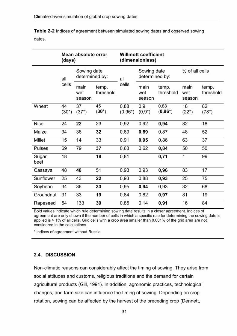
Climate-driven simulation of global crop sowing dates
Table 2-2 Indices of agreement between simulated sowing dates and observed sowing
dates.
Mean absolute error (days)
Willmott coefficient (dimensionless)
Sowing date determined by:
Sowing date determined by:
% of all cells
all cells
main wet season
temp. threshold
all cells
main wet season
temp. threshold
main wet season
temp. threshold
Wheat 44 (30*)
37 (37*)
45 (30*)
0,88 (0,96*)
0,9 (0,9*)
0,88 (0,96*)
18 (22*)
82 (78*)
Rice 24 22 23 0,92 0,92 0,94 82 18
Maize 34 38 32 0,89 0,89 0,87 48 52
Millet 15 14 33 0,91 0,95 0,86 63 37
Pulses 69 79 37 0,63 0,62 0,84 50 50
Sugar beet
18 18 0,81 0,71 1 99
Cassava 48 48 51 0,93 0,93 0,96 83 17
Sunflower 25 43 22 0,93 0,88 0,93 25 75
Soybean 34 36 33 0,95 0,94 0,93 32 68
Groundnut 31 33 19 0,84 0,82 0,97 81 19
Rapeseed 54 133 39 0,85 0,14 0,91 16 84
Bold values indicate which rule determining sowing date results in a closer agreement. Indices of agreement are only shown if the number of cells in which a specific rule for determining the sowing date is applied is > 1% of all cells. Grid cells with a crop area smaller than 0.001% of the grid area are not considered in the calculations.
* indices of agreement without Russia
2.4. DISCUSSION
Non-climatic reasons can considerably affect the timing of sowing. They arise from
social attitudes and customs, religious traditions and the demand for certain
agricultural products (Gill, 1991). In addition, agronomic practices, technological
changes, and farm size can influence the timing of sowing. Depending on crop
rotation, sowing can be affected by the harvest of the preceding crop (Dennett,
31

Climate-driven simulation of global crop sowing dates
1999), and available labour and machinery, depending on farm size, determine
whether sowing can be completed in the desired time period (Kucharik, 2006). The
timing of sowing may also be influenced by the weather later in the growing season,
e.g. in order to avoid possible dry spells during certain stages of crop development
that are relatively sensitive to drought stress. Information on these technological and
socio-economic conditions and their influence on the timing of sowing is scarce at
global scale and has therefore not been considered in this study. The results of our
study (Figure 2-4 and Figure A-1 to Figure A-11) show, however, that close
agreement between simulated and observed sowing dates for large parts of the Earth
for wheat, rice, millet, soybean, sugar beet and sunflower, as well as for pulses and
maize in temperate regions, can be realized based on climatic conditions only. For
most crops, the disagreement between simulated and observed sowing dates is only
1 month or less for the largest part of the global total cropping area (Figure 2-4b). At
least 80% of the global cropping area displays a disagreement of less than 2 months
(except for rapeseed, Figure 2-4b). However, some regions show mediocre or poor
agreement, between simulated and observed sowing dates. The agreement is
especially poor in tropical regions, where, despite a possible seasonality, climatic
conditions are favourable throughout the year and in regions characterized by
multiple cropping systems. Furthermore, agreement is poor in temperate regions,
where both spring and winter varieties of wheat and rapeseed are grown, and in
regions where observations are lacking or have been replaced or adjusted in
MIRCA2000.
In the sections below the most likely reasons for strong disagreements are identified
in example regions. Reasons can be limitations and uncertainties in MIRCA2000 e.g.:
the spatial scale of MIRCA2000 or data gaps; uncertainties in our methodology e.g.:
the usage of one global temperature threshold for sowing temperatures, which is
known to vary between regions (Sacks et al., 2010), or the application of specific crop
management techniques e.g. multiple cropping systems.
Pulses and groundnuts in multiple cropping systems
The poor agreement between simulated and observed sowing dates for pulses in
Southeast Asia, India, West and East Africa and Southeast Brazil, and for groundnuts
in India (Figure A-10a), originates from a mismatch in production systems assumed.
32

Climate-driven simulation of global crop sowing dates
In these regions, it is common practice to grow pulses and groundnuts in multiple
cropping systems. In the south-eastern region of Brazil, with rainy seasons long
enough for a multiple cropping system of maize and beans, bean is sown in
combination with maize or after maize has been harvested (Woolley et al., 1991). In
West and East Africa, cowpea is largely grown as a second crop in multiple cropping
systems with maize or cassava (in humid zones) and millet (in dry zones) (Mortimore
et al., 1997). These patterns are reflected in MIRCA2000. In contrast, we have
assumed only single-cropping systems, so that sowing of pulses and groundnut
starts at the beginning of the wet season, i.e. too early in comparison to the
observations. Where cowpea is grown as a single crop, as in coastal regions of East
Africa (Mortimore et al., 1997), there is close agreement with the observed sowing
dates (Figure A-5a).
The deviations in India for pulses (Figure A-5a), and for groundnut in western India
(Figure A-10a), are associated with the occurrence of multiple cropping systems.
Here, cowpea is grown in mixtures with sorghum and millet (Steele & Mehra, 1980)
and groundnuts may be grown in the dry season following rice, often under irrigation
(Norman et al., 1995b).
Maize in multiple cropping systems in Southeast Asia
In Southeast Asia, as well as in China, a large number of crops may be grown on the
same plot. According to Portmann et al. (2010), this indicates high land use
intensities with multiple cropping systems. Intensive rice and wheat production are
common practice in Asia (Devendra & Thomas, 2002), and maize has a subsidiary
place in some of the Asian cropping systems as a second crop following the wet-
season rice crop (Norman et al., 1995b). This rice-maize multiple cropping system is
covered by MIRCA2000, e.g. in China and Burma. As a consequence, the simulated
growing period of maize starts earlier in the year than the observed growing period
(Figure A-3a).
Wheat and rapeseed in temperate regions
The poor agreement for wheat and rapeseed in temperate regions of Russia,
Australia and small parts of Europe (Figure A-1a and Figure A-11a) is the result of
disagreement between the simulated and observed varieties of wheat and rapeseed.
33

Climate-driven simulation of global crop sowing dates
In Russia, MIRCA2000 overestimates the share of winter wheat (Portmann et al.,
2010), because the cropping calendar for Russia is partly derived from the cropping
calendars from Ukraine, Norway and Romania, where mainly winter wheat is grown
(Portmann et al., 2008). In contrast, we exclude winter wheat in Russia because
temperatures drop below 12°C before 15 September, and consequently spring wheat
is simulated in Russia. This is in line with the cropping calendar from USDA, which
reports in addition to winter wheat, large areas of spring wheat in Russia (U.S.
Department of Agriculture, 1994). In other temperate regions the agreement between
simulated and observed sowing dates is good with only one month deviation and
simulated sowing dates are similar to that shown in Bondeau et al. (2007).
For rapeseed in southern and eastern Australia, our rules simulate sowing dates in
May and June (Figure A-11b), whereas MIRCA2000 reports a sowing date in
December (Figure A-11c). However, in line with the simulations, West et al. (2001)
and Robertson et al. (2009) confirm that rapeseed is grown as a winter crop, starting
in May and June in Australia. In Europe, winter rapeseed is also the dominant cultivar
due to its higher yield levels. Sowing dates of winter rapeseed in southern Europe
can be extended from mid August to early September, as indicated by Booth &
Gunstone (2004) and USDA (1994), which is in line with the simulated sowing dates
in countries like, e.g., Spain, France, Hungary, Ukraine and Romania (Figure A-11b).
MIRCA2000, however, indentifies spring rapeseed sown in May in those countries.
Cassava in multiple cropping systems
MIRCA2000 reports that in China, Thailand and Vietnam, cassava is sown in March
as an early-ripening variety. In China, farmers plant cassava from February to April
before the rainy season starts in order to use the cover of cassava plants to avoid soil
losses due to the impact of heavy rains (Yinong et al., 2001). Planting before the
onset of the wet season may also avoid damage from pests (Evangelio, 2001). These
practices explain the differences in southern China and Southeast Asia between
observed and simulated sowing dates (Figure A-7a), because the simulated sowing
dates are associated with the main wet season starting in May to July, not with the
agronomic practices described in the literature.
34

Climate-driven simulation of global crop sowing dates
Specific climatic conditions in temperate regions
Other examples of differences between observed and simulated sowing dates occur
in European countries, partly in countries which are characterized by a
Mediterranean climate. For sugar beet, both MIRCA2000 and our simulations
indicate mainly spring-sowings in the Mediterranean region. However, the
Mediterranean climate is characterized by mild winters and winter rainfall. In those
regions, sugar beet is therefore sown in autumn, avoiding the high temperatures and
high evapotranspirational demand of summer (Castillo Garcia & Lopez Bellido, 1986;
Elzebroek & Wind, 2008; Rinaldi & Vonella, 2006). The effect of this specific climatic
condition on sowing dates is not reflected in MIRCA2000, or in our simulations.
Limitations of MIRCA2000
Large differences between observed and simulated sowing dates occur in countries
characterized by strong climatic gradients, associated with the size of countries (e.g.
Russia, DR Congo, Mexico), or to large climatic variability, associated with large
differences in elevation (e.g. Kenya). These gradients and variability influencing
sowing dates are captured in our methodology, but not in MIRCA2000, where sowing
dates for one spatial unit (country or sub-national unit) are assigned to grid cells of
0.5° by 0.5°. An example is the large difference between observations and
simulations in the southern part of the DR Congo, where in MIRCA2000 missing
observations were replaced by the cropping calendar from the neighbouring country
Rwanda (Portmann et al., 2008). While this procedure might be adequate for the
northern parts of the DR Congo which are characterized by the same bimodal
seasonal rainfall distribution, it is not adequate for the southern parts, where the main
wet season does not start until November/December (McGregor & Nieuwolt, 1998).
Deficiencies in simulated sowing dates may strongly influence results of applications
of the sowing date algorithm, depending on application and model used. A deviation
of sowing dates by 2 or 3 months (e.g. sunflower in France, sugar beet in Spain,
soybean in northern USA, or maize in Europe, see Figure A-1 to Figure A-11 in
Appendix A) could already strongly affect the results of crop model applications, e.g.
the assessment of crop evapotranspiration and crop virtual water content. The level
of agreement per crop and region is therefore depicted in Appendix A, which allows
for a more detailed evaluation of when to use our sowing date algorithm with caution.
35

Climate-driven simulation of global crop sowing dates
2.5. CONCLUSIONS
This study presents a novel approach for deterministically simulating sowing dates
under rainfed conditions for various annual field crops. We show that sowing dates
for large parts of the Earth can be satisfactorily estimated from climatic conditions
only. Close agreement is achieved between simulated and observed sowing dates,
although substantial deviations occur in: (1) tropical regions and (2) regions with high
land-use intensity and multiple cropping systems. Even if those regions show
seasonality in temperature or precipitation, climatic conditions can be suitable
throughout the year for crop growth. In both types of regions, climatic conditions are
of minor importance for the timing of sowing, instead it is determined mainly by other
criteria such as the demand for special agricultural products, availability of labor and
machines, and religious and/or social traditions (Gill, 1991; Kucharik, 2006).
Furthermore, certain cropping practices and crop rotations are applied in order to
avoid pests and disease infestations. These agronomic practises cannot be
considered in our methodology due to lack of information at global scale. Differences
between simulated and observed sowing dates in regions without precipitation and
temperature seasonality have little impact on the computed crop yield in global crop
growth models such as LPJmL. Sowing date deviations of one month or more, in
locations with temperature and precipitation seasonality may lead to substantially
different simulated crop yields. In the LPJmL model with the currently implemented
cultivars, sowing dates simulated with the presented methodology are within the most
productive cropping window for almost all locations displayed in Figure B-1. However,
the interaction of sowing dates, management options, and cultivar characteristics will
have to be evaluated further.
Our methodology is explicitly developed for the global scale. Climate and soil
characteristics, as well as agricultural management practices can vary considerably
among regions. If applied at smaller scales, parameter values as proposed here
should be adapted, e.g. the temperature threshold for sowing can show spatial
variability (Sacks et al., 2010), and important socio-economic and technical drivers
should be considered to attain higher accuracy. In addition, if reliable daily minimum
and maximum temperature and precipitation data are available, rules should adapted
in order to consider avoidance of damage by frost or extreme high temperature. At
global scale, our methodology is suitable for simulating sowing dates for global crop 36

Climate-driven simulation of global crop sowing dates
37
growth models. In our methodology, we are able to apply current and future climate
input data. We are therefore able to account for some possible global responses by
farmers to climate change in their sowing dates.
2.6. ACKNOWLEDGEMENTS
We would like to thank Felix Portmann and Stefan Siebert for making available the
MIRCA2000 data set, as well as the LPJmL crop modeling team, Herman van
Keulen, and Peter Leffelaar for valuable discussions on the methodology and results.
Furthermore we are grateful to Benjamin Gaede and Alison Schlums who did the
spell and grammar check. K.W. and C.M. gratefully acknowledge financial support
from projects with the International Food Policy Research Institute (6012001) and the
International Livestock Research Institute (81102850) funded through the German
Federal Ministry for Economic Cooperation and Development.
2.7. AUTHORS´ CONTRIBUTION
Authors´ contribution was as follows: K.W., L.vB, A.B. and C.M. conceived the idea of
simulating sowing dates from climatic conditions and from the intra-annual variability
of temperature and precipitation, K.W. and C.M. wrote code and prepared
MIRCA2000 for validation, K.W. did the model runs, derived the temperature
thresholds for sowing, and prepared the figures, L.vB carried out the sensitivity
analysis, and L.vB and K.W. did literature research, wrote the manuscript, and
prepared the supporting material. All authors were involved in developing the
methodology and discussing the model outputs.

38

3. Adaptation to climate change through the choice
of cropping system and sowing date in sub-
Saharan Africa
Our aim is to show the distribution of multiple cropping systems in sub-Saharan
Africa and analyse the susceptibility of traditional sequential cropping systems to
climate change. They provide more harvest security for farmers and allow for crop
intensification. Furthermore, the occurrence of multiple cropping systems will
influence ground cover, soil erosion, albedo, soil chemical properties, pest infestation
and the carbon sequestration potential. Comparing their productivity under climate
change to crop yields from alternative management strategies like growing a single
crop only or adapting the sowing date allows us to identify the most suitable
management strategy.
We identify the traditional sequential cropping systems composed of two crops
following one after another in ten sub-Saharan African countries from a dataset
containing more than 8600 household surveys. We design six different management
scenarios for adaptation to climate change and estimate crop yields for each of them.
The dynamic global vegetation model for managed land LPJmL (Bondeau et al.,
2007) is used to simulate crop yields under current and future climatic conditions
from three climate models for the SRES A2 and constant atmospheric CO2
concentrations.
We found that 13 different traditional sequential cropping systems were most
frequently applied in the study area. In 35% of all administrative units, at least one
sequential cropping system, mostly with groundnut or maize, is applied. Aggregated
mean crop yields in sub-Saharan Africa decrease by 6 % to 24 % due to climate
change depending on the climate model and the management strategy. The crop
yield decrease is typically weakest in sequential cropping systems and if farmers
adapt the sowing date to a changing climate. Crop calorific yields in single cropping
systems only reach 45 to 55 % of crop calorific yields obtained in sequential cropping
systems. Southern and Western Africa are the most heavily impacted regions with
declines in crop yield of up to 45 % and 18 % respectively depending on the
39

Adaptation to climate change through the choice of cropping system and sowing date in sub-
Saharan Africa
management scenario. As an exception, some traditional sequential cropping
systems in Kenya and South Africa gain by at least 25 %. In Cameroon, Kenya,
South Africa and Zimbabwe some of the traditional sequential cropping systems are
more resilient to negative climate change impacts than the highest-yielding
sequential cropping systems. As the farmers' choice of adequate crops, cropping
systems and sowing dates can be an important adaptation strategy to climate change
these management options should be considered in climate change impact studies
on agriculture.
This chapter is under review at Global Environmental Change as: Waha, K., Müller,
C., Bondeau, A., Dietrich, J.P., Kurukulasuriya, P., Heinke, J., Lotze-Campen, H.
Adaptation to climate change through the choice of cropping system and sowing date
in sub-Saharan Africa.
40

Adaptation to climate change through the choice of cropping system and sowing date in sub-
Saharan Africa
3.1. INTRODUCTION
The number of undernourished people remains highest in sub-Saharan Africa
compared to other world regions and population will be more than doubled in 2050
compared to 2000. Among effective strategies like fighting poverty, stabilizing
economies and ensure access to food, increased food production in smallholder
agriculture will be a key strategy for fighting hunger (FAO, 2008). Agricultural
production can be increased by expanding agricultural land and by increasing the
intensification of crop production through higher crop yields and higher cropping
intensities. The cropping intensity in less-developed countries can be increased by
about 5-10 % during the next 35 years if adequate amounts of input are available
(Döös & Shaw, 1999). Multiple cropping systems allow for this intensification by
growing two or more crops on the same field either at the same time or after each
other in a sequence (Francis, 1986b; Norman et al., 1995a). They already are
common farming systems in tropical agriculture today (Table 3-1). In multiple
cropping systems the risk of complete crop failure is lower compared to single
cropping systems and monocultures providing a high level of production stability
(Francis, 1986a). Furthermore the second crop in a sequence may benefits from an
increased amount of nitrogen derived from fixation (Bationo & Ntare, 2000; Sisworo
et al., 1990) or phosphorous from deep-rooted species (Francis, 1986a) as well as
from decreased disease pressure (Bennett et al., 2012) which helps to reduce the
use of mineral fertilizer and pesticides. Cropping intensity is not only important in
terms of agricultural production; the duration crops cover the soil will also influence
albedo, ground cover, carbon sequestration potential and soil erosion (Keys &
McConnell, 2005). In sub-Saharan Africa, multiple cropping systems mostly consist of
cereal-legume mixed cropping dominated by maize, millet, sorghum and wheat (Van
Duivenbooden et al., 2000). Maize- and cassava-based mixed cropping systems are
common in humid East and West Africa, whereas millet-based mixed cropping is
widely applied in dry East and West Africa (Francis, 1986b). Intercropping is the
traditional and most frequently applied multiple cropping system in sub-Saharan
Africa, however sequential cropping and mixed sequential cropping systems are also
common indigenous management practices (Table 3-1).
41

Adaptation to climate change through the choice of cropping system and sowing date in sub-
Saharan Africa
Table 3-1 Definition of terms used in this study.
Term Definition, Description
single cropping A cropping system with only one crop growing on the field (Bennett et al., 2012). Interchangeable with monoculture or continuous cropping.
sequential cropping A cropping system with two crops grown on the same field in sequence during one growing season with or without a fallow period. A specific case is double cropping with the same crop grown twice on the field.
mixed sequential cropping
A cropping system with two intercropping systems grown on the same field in sequence during one growing season with or without a fallow period.
growing period The period of time from sowing to maturity determined by the sum of daily temperatures above a crop-specific temperature threshold = phenological heat unit sum (PHU).
growing season The period of time in which temperature and moisture conditions are suitable for crop growth, in the sub-tropical and tropical zones determined by the start and end of the main rainy season.
multiple cropping “ […] may refer to either growing more than one crop on a field during the same time (intercropping), after each other in a sequence (sequential cropping) or with overlapping growing periods (relay cropping)” (Francis, 1986b; Norman et al., 1995a). Examples in sub-Saharan Africa are:
groundnut-millet succession in the northern part of central Africa (de Schlippe, 1956)
wheat-chickpea succession in Ethiopia (Berrada et al., 2006)
maize double cropping in western Nigeria (Francis, 1986b)
cowpea-maize sequence cropping in the moist Savannah zone of northern Nigeria (Carsky et al., 2001),
soybean and wheat sequences in Zimbabwe (Beets, 1982),
sorghum and pigeonpea in northern Nigeria (Francis, 1986a),
sorghum double cropping in southern Guinea and Savannah zones of West Africa (Kowal & Kassam, 1978).
42

Adaptation to climate change through the choice of cropping system and sowing date in sub-
Saharan Africa
Agricultural activities and consequently the livelihoods of people reliant on agriculture
will be affected by changes in temperature and precipitation conditions in large parts
of sub-Saharan Africa (Boko et al., 2007; Christensen et al., 2007; Müller et al.,
2011). Under climate change, many areas in sub-Saharan Africa are likely to
experience a decrease in the length of the growing season, while in some highland
areas rainfall changes may lead to a prolongation of the growing season (Thornton et
al., 2006). The degree of climate change impacts on agricultural production differs
between crops (Challinor et al., 2007; Liu et al., 2008; Schlenker & Lobell, 2010;
Thornton et al., 2011) and agricultural systems (Thornton et al., 2010). Therefore the
farmers' choice of an adequate cropping system and crop cultivar, especially in
precipitation-limited areas, might be an important adaptation strategy to changing
climate conditions (O´Brien et al., 2000; Thomas et al., 2007). Lobell et al. (2008)
note that the identification of practicable adaptation strategies for cropping systems
should be prioritized for regions impacted by climate change. However, few studies
investigate the impact of climate change on agriculture in sub-Saharan Africa
considering the cropping system applied or make an effort to identify the least
impacted cropping systems. The study of Thornton et al. (2009) is an exception,
analysing crop yield response to climate change of a maize-bean cropping sequence
in East Africa under which beans grow in a separate second growing season.
Analysing different multiple cropping systems in a climate impact study for sub-
Saharan Africa requires a dataset reporting their spatial distribution in the region,
which to our knowledge is not available. Some crop calendars available at the global
(Portmann et al., 2010; Sacks et al., 2010) or African scale (FAO, 2010) report the
growing periods of individual crops but lack reporting calendars for multiple cropping
systems, while some others only cover Asian regions (Frolking et al., 2006; Frolking
et al., 2002). Fischer et al. (2002b) identified potential double and triple cropping
zones by comparing temperature and moisture requirements of four crop groups with
climatic conditions worldwide. Thornton et al. (2006) developed a classification for
agricultural systems in Africa by combining a global livestock production classification
system, a farming system classification, and global land cover maps. Both datasets
do not report the crop cultivars or the cropping systems.
43

Adaptation to climate change through the choice of cropping system and sowing date in sub-
Saharan Africa
The knowledge about the spatial distribution of multiple cropping systems needs to
be expanded by more detailed information on the sub-national level. We analyse a
household survey (Dinar et al., 2008) carried out in 385 districts and provinces
containing more than 8600 households in ten countries of sub-Saharan Africa to fill
this gap. From this survey we are able to identify the traditional rainfed sequential
cropping systems with two crops grown within one year. As these are advantageous
management strategies because they allow for risk spreading and increased crop
productivity, we test their susceptibility to future climatic conditions in comparison to
alternative management strategies by simulating crop yields with the dynamic global
vegetation model for managed land LPJmL (Bondeau et al., 2007). We analyse the
ability of each management strategy to maximize future crop productivity or lower
negative impacts from climate change on crops. We perform this analysis in locations
where sequential cropping systems are already applied by local farmers today and
also for the entire region of sub-Saharan Africa in order to estimate potential benefits.
3.2. MATERIALS AND METHODS
Input data for current and future climate
To describe current climatic conditions, we used time series of monthly temperature
and precipitation as well as the number of wet days from the climate database
CRU TS 3.0 (Mitchell & Jones, 2005) for the 30-year period 1971 to 2000 on a spatial
resolution of 0.5° x 0.5°. Future climatic conditions for the 30-year period 2070-2099
were projected from the three Global Circulation Models (GCMs) ECHAM5
(Jungclaus et al., 2006), HadCM3 (Cox et al., 1999), and CCSM3 (Collins et al.,
2006) under the SRES A2 emission scenario. As there is little consistency between
GCM projections on precipitation (Boko et al., 2007) they were chosen to show a
wide range of possible future precipitation patterns (Fig. 1). The monthly mean
temperature and precipitation sums from these three GCMs were interpolated to a
finer spatial resolution of 0.5° x 0.5° using bilinear interpolation and smoothed using a
30-year running mean. The temperature and precipitation anomalies from each GCM
were calculated relative to the 1971-2000 average climate from CRU TS 3.0 and
were then applied to this baseline while preserving observed variability (Gerten et al.,
2011). Daily mean temperatures were obtained by linear interpolation between mean
monthly temperatures, and daily precipitation data was provided by a weather
44

Adaptation to climate change through the choice of cropping system and sowing date in sub-
Saharan Africa
generator which distributes monthly precipitation to the number of observed wet days
in a month, considering the transition probabilities between wet and dry phases
(Geng et al., 1986; Gerten et al., 2004). We kept the number of wet days constant at
their average number from the time period 1971-2000. Geng et al. (1986) confirms
that the rainy days as well as the amount of precipitation generated from this
procedure are in general very close to observations in different environments. In this
analysis we keep atmospheric CO2 concentrations constant at 370 ppm. Increasing
atmospheric CO2 concentrations can increase the productivity of plants (especially C3
plants), but the effectiveness on increasing crop yields is uncertain (Long et al., 2006;
Tubiello et al., 2007) and does require adaptation in management (Ainsworth & Long,
2005).
Figure 3-1 Change in annual mean temperature and annual mean precipitation from
1971-2000 to 2070-2099 projected from three GCMs under the SRES A2. Brown and green
colours in the lower three panels indicate a decrease or an increase in annual mean
precipitation respectively.
45
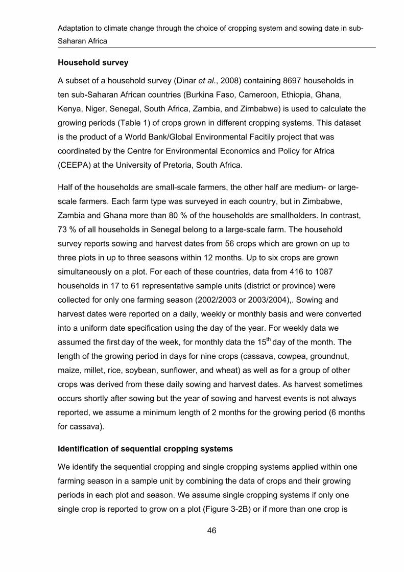
Adaptation to climate change through the choice of cropping system and sowing date in sub-
Saharan Africa
Household survey
A subset of a household survey (Dinar et al., 2008) containing 8697 households in
ten sub-Saharan African countries (Burkina Faso, Cameroon, Ethiopia, Ghana,
Kenya, Niger, Senegal, South Africa, Zambia, and Zimbabwe) is used to calculate the
growing periods (Table 1) of crops grown in different cropping systems. This dataset
is the product of a World Bank/Global Environmental Facitily project that was
coordinated by the Centre for Environmental Economics and Policy for Africa
(CEEPA) at the University of Pretoria, South Africa.
Half of the households are small-scale farmers, the other half are medium- or large-
scale farmers. Each farm type was surveyed in each country, but in Zimbabwe,
Zambia and Ghana more than 80 % of the households are smallholders. In contrast,
73 % of all households in Senegal belong to a large-scale farm. The household
survey reports sowing and harvest dates from 56 crops which are grown on up to
three plots in up to three seasons within 12 months. Up to six crops are grown
simultaneously on a plot. For each of these countries, data from 416 to 1087
households in 17 to 61 representative sample units (district or province) were
collected for only one farming season (2002/2003 or 2003/2004),. Sowing and
harvest dates were reported on a daily, weekly or monthly basis and were converted
into a uniform date specification using the day of the year. For weekly data we
assumed the first day of the week, for monthly data the 15th day of the month. The
length of the growing period in days for nine crops (cassava, cowpea, groundnut,
maize, millet, rice, soybean, sunflower, and wheat) as well as for a group of other
crops was derived from these daily sowing and harvest dates. As harvest sometimes
occurs shortly after sowing but the year of sowing and harvest events is not always
reported, we assume a minimum length of 2 months for the growing period (6 months
for cassava).
Identification of sequential cropping systems
We identify the sequential cropping and single cropping systems applied within one
farming season in a sample unit by combining the data of crops and their growing
periods in each plot and season. We assume single cropping systems if only one
single crop is reported to grow on a plot (Figure 3-2B) or if more than one crop is
46

Adaptation to climate change through the choice of cropping system and sowing date in sub-
Saharan Africa
grown on a plot but the sum of their growing periods is larger than 365 days and/or
their growing periods overlap by more than 15 days (Figure 3-2C, Figure 3-2A), i.e.
the growing period a crop is not restricted by the occurrence of other crops on that
plot. In contrast, we assume sequential cropping systems if two crops are reported to
be planted one after another without overlaps of more than 15 days and if their
growing periods sum up to less than 365 days (Figure 3-2D-G), i.e. the growing
period of a crop here is restricted by the occurrence of the associated crop on the
plot.
Figure 3-2 Scheme of possible timing and length of growing periods of crops in single
cropping systems (A-C) and sequential cropping systems (D-G) according to the definition
used in this study. A: two single cropping systems with large overlap, B: one single cropping
system, C: two single cropping systems, one spanning the turn of the year and with the sum
of the growing periods exceeding 365 days, D: sequential cropping system with small
overlap, E: sequential cropping system with long fallow period, F: sequential cropping system
with short or no fallow period, G: sequential cropping system spanning the turn of the year
with sum of growing periods below 365 days.
An overlap of 15 days corresponds to the maximum possible error in sowing and
harvest dates owing to the conversion from monthly to daily data. We only consider
47

Adaptation to climate change through the choice of cropping system and sowing date in sub-
Saharan Africa
rainfed systems in this study because irrigation systems are rarely available in sub-
Saharan Africa. If various sequential cropping systems exist within a district, we
identify the most frequently applied sequential cropping system in a district and
assume this system to be the traditionally applied sequential cropping system. Based
on the distance between the centre coordinates of the districts and those of the
0.5° x 0.5° grid cells, the sequential cropping systems found in a district are allocated
to the closest grid cell. If a district covers more than one grid cell the sequential
cropping systems are distributed to all corresponding grid cells.
Management scenarios for adaptation
Farmers choose a cropping system according to economic market trends, consumer
demands, availability of inputs such as seeds, fertilizer and pesticides, agronomy
traditions as well as current land-use, climatic conditions and soil properties (Bennett
et al., 2012; Castellazzi et al., 2008) in order to maximize their yield and profit and/or
to minimize the risk of crop failure through diversification. Rainy seasons long enough
for growing two crops in a sequential cropping system allow for intensification and
more harvest security for farmers because crop yields are obtained two or more
times a year (Andrews & Kassam, 1976). If necessary, farmers respond to perceived
changes and variability in climate by e.g. changing the sowing date of cultivated
crops or switching to a more suitable crop or crop cultivar with a different growing
period, heat tolerance or drought resistance. These strategies were already observed
in Tanzania (O´Brien et al., 2000), semi-arid West Africa (Mation & Kristjanson,
1988), and South Africa (Benhin, 2006). It can thus be expected that farmers will
adapt their traditional cropping system to a changing climate to some extent. We
define three management scenarios, analyzing different cropping system with the aim
of comparing changes in crop yields with changing climate of the 21st century in order
to find the most suitable strategy:
TS: Traditional sequential cropping system: The baseline strategy. Farmers grow
the sequential cropping system most frequently applied in their district composed
of two short-growing crop cultivars.
SC: Single cropping system: Farmers only grow one long-growing cultivar of the
first crop of the traditional sequential cropping system.
48

Adaptation to climate change through the choice of cropping system and sowing date in sub-
Saharan Africa
HS: Highest-yielding sequential cropping system: Farmers grow the sequential
cropping system composed of two short-growing crop cultivars with the highest
yields.
Sowing dates in these scenarios change dynamically, with changes in the start of the
main rainy season allowing for inter-annual variability. In order to assess the
importance of adapting sowing dates to changing climate or weather conditions three
additional scenarios are designed in which the sowing dates are kept constant with
the simulated sowing dates in the first simulation year 1971.
TSco: Traditional sequential cropping system as described above with constant
sowing dates.
SCco: Single cropping system as described above with constant sowing dates.
HSco: Highest-yielding sequential cropping system as described above with
constant sowing dates.
Accordingly, each of the six management scenarios is a combination of a specific
cropping system and sowing date setting, as these are important management
options for farmers.
We assume that farmers prefer short-growing crop cultivars in sequential cropping
systems in order to reduce the risk of crop failure in the second half of the growing
season (Table 1) or, alternatively, long-growing crop cultivars in single cropping
systems in order to increase the yield. Sequential cropping systems are
advantageous farming systems but cannot be applied if the growing season is too
short. In this case a single cropping system may be the most suitable cropping
system. Adapting sowing dates to shifts in the start of the rainy season ensures
optimal growing conditions and low risk of drought at important crop growth stages
and, therefore, allows for better use of rainwater and potentially increased crop yields
(Van Duivenbooden et al., 2000).
Dynamic global vegetation model for managed land LPJmL
LPJmL is a process-based global vegetation model for natural and agricultural
vegetation, simulating biophysical and biogeochemical processes as well as
49

Adaptation to climate change through the choice of cropping system and sowing date in sub-
Saharan Africa
productivity and yield of the most important crops (Bondeau et al., 2007; Sitch et al.,
2003). Carbohydrates from photosynthesis are allocated to different crop organs at
daily time steps depending on the phenological stage of the crop and environmental
conditions. To simulate the phenological development of a crop, the heat unit theory
is applied (Bondeau et al., 2007). Heat units (in degree-days [°Cd]) are calculated
from daily temperatures above a base temperature (Table 2) and are summed over
all phenological stages (potential heat unit sum, PHU [°Cd]). This empirically derived
quantitative measurement describes the effect of air temperature on the growth of
crops (Boswell, 1926) and reflects the length of a crop’s growing period.
Temperature and water stress influence crop development and growth (Bondeau et
al., 2007). Increasing temperatures lead to a shortened growing period because
crops reach maturity earlier in the year and crop yields potentially decrease. Stress
due to extreme temperatures does not damage the crop irreversibly in the model, but
temperatures beyond the optimal temperatures for photosynthesis reduce
productivity. A water stress factor is calculated from the ratio of water supply through
plant water uptake from the soil and atmospheric water demand (Sitch et al., 2003)
and influences leaf growth (Bondeau et al., 2007). We extended this approach to also
account for changes in root growth in response to water stress (Appendix C). Water
stress effecting leaf and root growth negatively might occur more frequently in the
second crop cycle because water stored in the soil was already consumed by the
preceding crop.
It is possible to simulate different crop cultivars with LPJmL for wheat and rapeseed
(spring and winter cultivar), as well as for maize and sunflower (temperate and
tropical cultivar) by varying the PHU (Bondeau et al., 2007). We extend this approach
by calculating PHUs for a short-growing crop cultivar grown in sequential cropping
systems (PHUseq) and a long-growing crop cultivar grown in single cropping systems
(PHUsin) from observed growing periods and daily temperatures in sub-Saharan
Africa. The base temperatures are taken from LPJmL (Bondeau et al., 2007) for
groundnut, millet, rice, soybean, sunflower and wheat and from SWAT (Neitsch et al.,
2002) for cassava, cowpea and maize (Table 2).
50

Adaptation to climate change through the choice of cropping system and sowing date in sub-
Saharan Africa
The start of the growing season in subtropical and tropical environments is
determined by the start of the main rainy season and is simulated dynamically in
LPJmL from monthly climatology (Waha et al., 2012). This procedure follows the
commonly used approach of identifying the onset and end of the rainy season with a
criterion based on the average rainfall or radiation of a specific period, e.g. 5 days
(Marengo et al., 2001; Omotosho et al., 2000; Wang & Ho, 2002). In slight contrast to
the methodology described in Waha et al. (2012) for the global scale, this criterion is
defined here as the three-month averaged ratio between precipitation and potential
evapotranspiration:
where P/PET is the mean three-month averaged precipitation-to-potential
evapotranspiration ratio, P/PETm is the precipitation-to-potential evapotranspiration
ratio of each individual month m. Potential evapotranspiration is calculated in LPJmL
using the Priestley-Taylor equations (Priestley & Taylor, 1972) with a Priestley-Taylor
coefficient of 1.391 (Gerten et al., 2004).
Consequently, the onset of the growing season is defined as the first month in a
three-month period where precipitation-to-potential-evapotranspiration ratios exceed
the mean ratio. Within this month the growing period of an individual crop starts at the
first wet day with daily precipitation above 0.1mm; in sequential cropping systems the
following crop is assumed to be sown immediately after the harvest of the first crop.
In temperate environments such as parts of South Africa, the start of the growing
season is determined by daily temperature as described in Waha et al. (2012). The
start of the main rainy season in sub-Saharan Africa as simulated here agrees well
with the observed start of the main growing season derived from satellite data
(Appendix D).
The growing period is limited to a maximum of 330 days allowing for a short fallow
period between two consecutive years. The simulated harvested carbon in gC/m² is
converted to crop yield in Mcal/ha to allow for a comparison between crops and
cropping systems with:
51
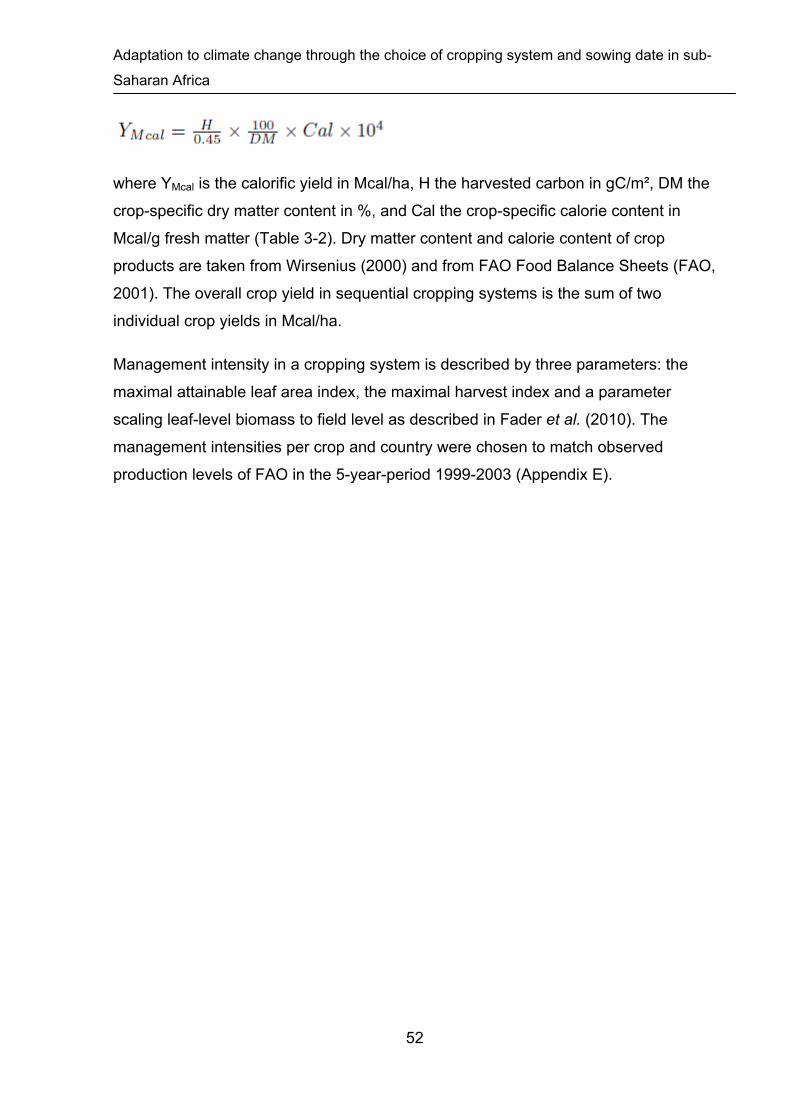
Adaptation to climate change through the choice of cropping system and sowing date in sub-
Saharan Africa
52
where YMcal is the calorific yield in Mcal/ha, H the harvested carbon in gC/m², DM the
crop-specific dry matter content in %, and Cal the crop-specific calorie content in
Mcal/g fresh matter (Table 3-2). Dry matter content and calorie content of crop
products are taken from Wirsenius (2000) and from FAO Food Balance Sheets (FAO,
2001). The overall crop yield in sequential cropping systems is the sum of two
individual crop yields in Mcal/ha.
Management intensity in a cropping system is described by three parameters: the
maximal attainable leaf area index, the maximal harvest index and a parameter
scaling leaf-level biomass to field level as described in Fader et al. (2010). The
management intensities per crop and country were chosen to match observed
production levels of FAO in the 5-year-period 1999-2003 (Appendix E).

Table 3-2 Crop-specific parameters for estimating PHUs in single and sequential cropping systems and calculating fresh matter crop yields
in kcal/ha.
Parameters for estimating PHUsin and PHUseq in LPJmL
Dry matter DM c and calorie content Cal d
Crop Base tempera
turea,b [°C]
α [°Cd] β [d] γ [°Cd/
mm]
δ [°Cd/
mm]
R R N H2 Min PHUsin
[°Cd]
Max PHUsin
[°Cd]
P Ugap [-] ‡ N DM
[%]Cal
[kcal/
g]
Cassava 14 -4910 327 0.5 -0.6 0.75 0.56 910 4510 213 0.67 ± 0.26 *** 50 35 1.09
Cowpea 14 -470 44 -0.2 0.9 0.58 0.34 740 1910 190 0.75 ± 0.21 *** 33 90 3.41
Groundnut 14 470 32 -0.2 0.4 0.48 0.23 1070 1990 336 0.99 ± 0.29 * 117 94 4.14
Maize 8 1740 0.1 -0.1 0.7 0.48 0.23 1880 3640 472 0.92 ± 0.21 *** 224 88 3.56
Rice 10 250 21 0 1.3 0.65 0.42 1450 2700 102 0.88 ± 0.19 * 16 87 2.80
Wheat 0 -390 146 0.8 -0.2 0.76 0.58 2180 4310 61 0.87 ± 0.34 * 26 88 3.34
a Bondeau et al. (2007), b Neitsch et al. (2002), c Wirsenius (2000), d FAO (2001). ‡ Values are means ± standard deviation for PHUgap. Level of significance (*** p<0.001, ** p<0.01, and * p<0.05) is given for the hypothesis that PHUseq < PHUsin (Wilcoxon signed-rank test).

Adaptation to climate change through the choice of cropping system and sowing date in sub-
Saharan Africa
54
Modelling the spatial variation of PHUsin and PHUseq
PHUsin and PHUseq are calculated by accumulating daily temperatures above a base
temperature threshold (Table 3-2) summed over the growing period that is reported in
the household survey. In order to estimate PHUsin for each crop in each grid cell in
sub-Saharan Africa, we use a multiple linear regression model between PHUsin and
climatic parameters in each grid cell. We found a correlation, although light, for maize
and groundnut, between PHUsin, mean annual temperature and moisture conditions
during the growing season:
where T is the annual mean temperature, Pgs the sum of monthly precipitation during
the growing season, PETgs the sum of monthly potential evapotranspiration during the
growing season, and α, β, γ and δ are empirical parameters.
Precipitation and potential evapotranspiration represent the atmospheric water supply
and water demand, respectively. Thus their ratio in the growing season represents
the water availability during the period of high agricultural activity.
We compare PHUsin and PHUseq with the aim of verifying the assumption that farmers
apply short-growing crop cultivars in sequential cropping systems and long-growing
crop cultivars in single cropping systems. We test if PHUsin is statistically greater than
PHUseq for each crop using the non-parametric Wilcoxon signed-rank test (Wilcoxon,
1945). In order to estimate PHUseq for each crop in each grid cell, we derive a uniform
crop-specific factor PHUgap from the calculated PHUsin and PHUseq to account for the
deviation between them:
Theoretical potential of sequential cropping systems
In addition to the analysis of climate change impacts on crop yields in districts where
sequential cropping systems are already grown, we apply a similar analysis to the
entire region of sub-Saharan Africa that currently has growing periods larger than 5
months (Harvest Choice, 2011) to analyze the adaptation potential of sequential

Adaptation to climate change through the choice of cropping system and sowing date in sub-
Saharan Africa
55
cropping systems. Crop yields from 13 sequential cropping systems and six single
cropping systems are simulated with LPJmL and compared in all sub-Saharan Africa
grid cells that are currently used for crop production following Fader et al. (2010).
3.3. RESULTS
Sequential cropping systems in sub-Saharan Africa
In 35 % of the surveyed districts one or more sequential cropping system exist, but
only in seven out of ten surveyed countries and about 17 % of the districts sequential
cropping systems are composed of crops included in our model. Figure 3-3 shows
the distribution of the 13 traditional sequential cropping systems in the surveyed
districts. The sequential cropping systems frequently applied are mostly based on
groundnut and maize and to a smaller extent also on cassava, rice, wheat, and
cowpea, but only few sequential cropping systems exist with sunflower or soybean,
which are of minor importance in the surveyed households. In Eastern Africa all
sequential cropping systems are based on maize, whereas in Southern Africa wheat-
maize systems are additionally applied. Systems based on groundnut as the first crop
can be found in Ghana and in Cameroon, which is the country with the highest
diversity in sequential cropping systems. The highest-yielding among all 13 traditional
sequential cropping systems are mostly based on maize (Table 3-3).

Adaptation to climate change through the choice of cropping system and sowing date in sub-
Saharan Africa
56
Figure 3-3 Most frequently applied rainfed sequential cropping systems in sub-Saharan
Africa. The classification of sequential cropping systems used for legend titles is based on
the first crop grown in the sequence.
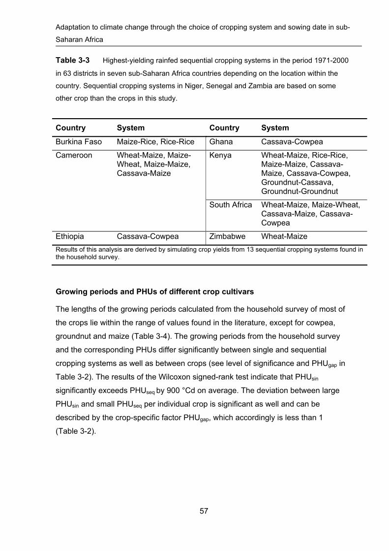
Adaptation to climate change through the choice of cropping system and sowing date in sub-
Saharan Africa
57
Table 3-3 Highest-yielding rainfed sequential cropping systems in the period 1971-2000
in 63 districts in seven sub-Saharan Africa countries depending on the location within the
country. Sequential cropping systems in Niger, Senegal and Zambia are based on some
other crop than the crops in this study.
Country System Country System
Burkina Faso Maize-Rice, Rice-Rice Ghana Cassava-Cowpea
Kenya Wheat-Maize, Rice-Rice, Maize-Maize, Cassava-Maize, Cassava-Cowpea, Groundnut-Cassava, Groundnut-Groundnut
Cameroon Wheat-Maize, Maize-Wheat, Maize-Maize, Cassava-Maize
South Africa Wheat-Maize, Maize-Wheat, Cassava-Maize, Cassava-Cowpea
Ethiopia Cassava-Cowpea Zimbabwe Wheat-Maize
Results of this analysis are derived by simulating crop yields from 13 sequential cropping systems found in the household survey.
Growing periods and PHUs of different crop cultivars
The lengths of the growing periods calculated from the household survey of most of
the crops lie within the range of values found in the literature, except for cowpea,
groundnut and maize (Table 3-4). The growing periods from the household survey
and the corresponding PHUs differ significantly between single and sequential
cropping systems as well as between crops (see level of significance and PHUgap in
Table 3-2). The results of the Wilcoxon signed-rank test indicate that PHUsin
significantly exceeds PHUseq by 900 °Cd on average. The deviation between large
PHUsin and small PHUseq per individual crop is significant as well and can be
described by the crop-specific factor PHUgap, which accordingly is less than 1
(Table 3-2).

Adaptation to climate change through the choice of cropping system and sowing date in sub-
Saharan Africa
58
Table 3-4 Time from sowing to harvest in months for different crop cultivars found in the
household survey and in literature.
Crop Household survey Literature
Cassava 6 – 11 6 – 24 (Alves, 2002)
Cowpea 2 – 9 ½ 1 ½ – 6 (FAO, 2010; Madamba et al., 2006)
Groundnut 2 – 10 ½ 2 ½ – 6 (Ntare, 2006; Schilling & Gibbons, 2002; Virmani & Singh, 1986)
Maize 2 – 9 2 ½ – 6 ½ (Badu-Apraku & Fakorede, 2006)
Rice 2 – 6 ½ 3 – 7 (Badu-Apraku & Fakorede, 2006; Meertens, 2006)
Wheat 3 – 6 3 – 5 ½ (Belay, 2006; FAO, 2010; Rehm & Espig, 1991)
Using the multiple regression model to determine the heat sum requirements for
phenological development, simulated growing periods from LPJmL differ from
growing periods in the household survey: for wheat, rice and cowpea, simulated
growing periods are on average 5 to 32 days shorter than the growing periods in the
household survey, while those for groundnut, cassava and maize are on average 7 to
33 days longer than the growing periods reported in the household survey (Figure 3-
4).

Adaptation to climate change through the choice of cropping system and sowing date in sub-
Saharan Africa
59
Figure 3-4 Deviations in days between simulated and observed length of growing period
in 2002/03 in single cropping systems (observed – simulated). Each box stretches from the
0.25-quantile to the 0.75-quantile of deviation with the bold line showing the 0.5-quantile of
deviations. Whiskers show the 1.5-fold interquartile range and points indicate individual
outliers.
Changes in crop yields
Decreasing crop yields
Future crop yields averaged over all locations contained in the household survey
(Figure 3-3) decrease between 6 % and 24 % because of climate change depending
on the GCM and management scenario (Table 3-5). The decrease is always weakest
in the management scenarios with traditional sequential cropping systems. There are
differences in mean crop yields and crop yield changes between the three GCMs,
with the highest crop yields under CCSM3 and the lowest under ECHAM5. Southern
and Western Africa are the most heavily impacted regions with declines in crop yield
of up to 45 % and 18 % respectively depending on the management scenario
(Figure 3-5). However, impacts in Southern Africa are diverse and crop yields in
some locations also increase by up to 6 % in the TS scenario.

Adaptation to climate change through the choice of cropping system and sowing date in sub-
Saharan Africa
60
Figure 3-5 Mean crop yields [Mcal/ha] per region in 1971-2000 and in 2070-2099 if
TS/TSco (the traditional sequence cropping systems), SC/SCco (only the first crop of the
traditional sequential cropping systems), or HS/HSco (the highest-yielding sequential
cropping systems) are applied, “co” indicates management scenarios with constant sowing
dates (as computed for the first simulation year 1971). Vertical lines show the range of
minimum to maximum crop yield from three GCMs. The countries of Zimbabwe and South
Africa are combined into the region Southern Africa, Kenya and Ethiopia are combined into
Eastern Africa and Burkina Faso, Cameroon and Ghana are combined into Western Africa.
Some traditional sequential cropping systems based on rice in Burkina Faso and
based on groundnut in Ghana and Cameroon are most heavily impacted, with crop
yield declines by at least 25 % (Table F-1 in Appendix F). In contrast, some traditional
sequential cropping systems based on maize and wheat in Kenya and South Africa
gain by at least 25 %. Mean future crop yields are higher (+ 11-17 %) in the TS, SC

Adaptation to climate change through the choice of cropping system and sowing date in sub-
Saharan Africa
61
and HS scenarios with adapted sowing dates compared to the corresponding TSco,
SCco and HSco scenarios with constant sowing dates (Table 3-5). As an exception,
crop productivity in some single and sequential cropping systems in management
scenarios with constant sowing dates is higher than in scenarios with adapted sowing
dates (Table F-1).
Table 3-5 Mean crop yields and crop yield changes per GCM and management scenario
in 63 districts of seven sub-Saharan Africa countries in the period 2070-2099 compared to
the period 1971-2000 in six management scenarios.
Crop yield 1971-2000 [Mcal/ha]
Crop yield 2070-2099 [Mcal/ha]
Management
Scenario
ECHAM5, HadCM3, CCSM3
ECHAM5 HadCM3
CCSM3
SCco 6660 5041 (-24%) 5459 (-18%) 5669 (-15%)
SC 7203 5894 (-18%) 6399 (-11%) 6393 (-11%)
TSco 10748 8942 (-17%) 9427 (-12%) 9799 (-9%)
TS 11564 10132 (-12%) 10677 (-8%) 10927 (-6%)
HSco 14435 11180 (-23%) 11676 (-19%) 12688 (-12%)
HS 15368 12796 (-17%) 13266 (-14%) 14095 (-8%)
TS/TSco: Traditional sequential cropping system, SC/SCco: Single cropping system, HS/HSco: Highest-yielding sequential cropping system, “co” indicating management scenarios with constant sowing dates
Sequential cropping systems vs. single cropping systems
Crop calorific yields in management scenarios with single cropping systems
(SC/SCco) only reach 45 to 55 % of crop calorific yields obtained in management
scenarios with sequential cropping systems (TS/TSco and HS/HSco) averaged over
all locations contained in the household survey (Table 3-5). As an exception, the
single cropping systems (SC/SCco) with maize in Kenya and South Africa yield
higher in some locations than the traditional sequential cropping system, but only
under current climatic conditions (Table F-1).

Adaptation to climate change through the choice of cropping system and sowing date in sub-
Saharan Africa
62
Crop yields in the highest-yielding sequential cropping systems (HS) exceed crop
yields in the traditional sequential cropping systems (TS) by 24 to 28 % depending on
the GCM (Table 3-5). However, frequently the traditional sequential cropping systems
are more resilient against negative climate change impacts than the highest-yielding
sequential cropping systems like e.g. groundnut-cassava systems in Cameroon,
maize-maize systems in some locations in Kenya, wheat-maize systems in some
locations in South Africa and maize-wheat systems in Zimbabwe (Table F-1).
Potential of sequential cropping systems in sub-Saharan Africa
If only the most stable sequential cropping systems would be chosen everywhere in
sub-Saharan Africa, crop yields would be also less impacted by climate change than
crop yields in single cropping systems in many locations (Figure 3-6). Crop yields in
both systems mostly decline, most severely in western Mali, southern Mauritania and
Senegal, but increase in small parts of South Africa, Kenya and Ethiopia. However, in
the last-mentioned locations there is also the highest variability of climate change
impacts on crop yields. The single cropping systems least impacted by climate
change are cassava and maize, and to a smaller extent also rice. The sequential
cropping systems least impacted are groundnut-cassava, rice-maize systems, but
also maize-maize and maize-groundnut.

Adaptation to climate change through the choice of cropping system and sowing date in sub-
Saharan Africa
63
Figure 3-6 Mean crop yield changes (%) in 2070-2099 compared to 1971-2000 with
corresponding standard deviations (%) in six single cropping systems (upper panel) and 13
sequential cropping systems (lower panel). Maps in the last column show the systems with
lowest crop yield declines or highest crop yields increases. White areas in sub-Saharan
Africa are excluded because the crop area is smaller than 0.001 % of the grid cell area or the
growing season length is less than five months. The high standard deviation in Southern
Africa is mainly determined by the large difference in climate projections.

Adaptation to climate change through the choice of cropping system and sowing date in sub-
Saharan Africa
64
3.4. DISCUSSION
Changes in crop yield
Crop yield decreases, mostly for single cropping systems, were also reported by
other studies (Jones & Thornton, 2003; Lobell et al., 2008; Schlenker & Lobell, 2010;
Thornton et al., 2011). Lobell et al. (2008) show declines in crop yield by up to 30%
for maize in Southern Africa, millet in Central Africa and cowpea in Eastern Africa as
early as 2030. In contrast to our results, Thornton et al. (2011) report higher mean
production decreases for maize in 2090 in Western Africa than in Southern Africa, but
in line with our results they project higher declines than in Eastern Africa. However, a
comparison between these results and our study is difficult due to different time
horizons, methodological approaches, climate projections and crop parameterization.
Mean crop yield decreases on average are most severe in Western and Southern
Africa due to climate change (Table 3-6). Increasing annual temperatures in all
regions lead to an accelerated phenological development and thus reduce growing
periods by 31 to 65 days. Furthermore, growing season precipitation decreases in
Southern Africa indicating a higher risk of water stress, in contrast to Eastern Africa
with considerable increases in growing season precipitation. Water stress during the
growing period affects photosynthesis as well as leaf and root growth, depending on
the phenological stage (Figure C-1 in Appendix C). Therefore, total biomass as well
as the biomass of harvested crop organs is reduced, depending on the crop type and
cropping system. In contrast, in the temperate zone of South-East Africa precipitation
is projected to increase or to remain constant from all three GCMs, leading to
increased crop yields in some traditional sequential cropping systems (Figure 3-5)
and also in some single cropping systems (Table F-1).

Adaptation to climate change through the choice of cropping system and sowing date in sub-
Saharan Africa
65
Table 3-6 Change in climate and length of the crops´ growing period in the period 2070-
2099 compared to the period 1971-2000 in six management scenarios using climate
projections from three GCMs.
Southern Africa Eastern Africa Western Africa
ECHAM5
Change in annual temperature [°C]
Change in annual precipitation [%]
Change in growing season precipitation [%] a
Change in length of crops´ growing period b
4,1
-4,9
-3,3
-65 days (-23%)
3,8
+11,4
+11,4
-35 days (-14%)
3,8
+12,0
+4,0
-36 days (-18%)
HadCM3
Change in annual temperature [°C]
Change in annual precipitation [%]
Change in growing season precipitation [%] a
Change in length of crops´ growing period b
4,4
-7,0
-6,2
-60 days (-22%)
3,6
+9,7
+12,8
-31 days (-12%)
3,8
-0,4
+0,4
-36 days (-18%)
CCSM3
Change in annual temperature [°C]
Change in annual precipitation [%]
Change in growing season precipitation [%] a
Change in length of crops´ growing period b
3,6
+11,1
+11,0
-43 days (-15%)
3,1
+24,8
+24,7
-29 days (-12%)
3,3
+6,8
+0,5
-31 days (-15%)a growing season as indicated from satellite data providing the time of greening-up and greening down (HarvestChoice, 2010) b growing period as simulated from LPJmL for different crops in six management scenarios

Adaptation to climate change through the choice of cropping system and sowing date in sub-
Saharan Africa
66
Farmers can lower the negative impact of changing climate on crop yields by
adapting the sowing date to the start of the main rainy season, which is already done
in many locations today. Simulation studies in Cameroon indicated that crop yields of
maize and groundnut under climate change with an optimal planting date are higher
compared to crop yields obtained using traditional planting dates, except for
groundnut at one location (Laux et al., 2010; Tingem & Rivington, 2009). This is in
agreement with our findings, as the adaptation of sowing dates in our study usually
results in higher crop productivity in these locations (Table 3-7). The benefits from
adapted sowing dates are even higher in the literature, as both studies optimize the
sowing date in order to maximize crop yields whereas in this study the sowing date is
adapted to a shifted start of the rainy season.
Table 3-7 Comparison of simulated crop yields from literature and this study.
Locationa, crop Reference Change to baseline,
without adaptation
Change to baseline,
with adaptation
Deviation between yield
without and with adaptation
Tiko/Moungo, groundnut
Tingem & Rivington (2009)
-5.1 % +28.9 % -
this study -25-29 % -22-21 % -
Ngaoundere/Vina, maize
Laux et al. (2010)
- - +1%
this study -19 % -14-15% +10.4-12.3%
Bamenda/Mbam and Bui, maize
Laux et al. (2010)
- - +16 %
this study -11-12 % -12 % -1.8- +2.9 %
Bamenda/Mbam and Bui, groundnut
Laux et al. (2010)
- - -9 %
this study -38 % -32 % +9.2 %
a locations in literature studies or related district in this study, e.g. the neighbouring district(s)
Attention should be paid to the different GCMs used in the studies in the literature and in this study. Crop yields from literature are shown for only one GCM (GISS), whereas in this study the results from three different GCMs are averaged. The SRES scenario and time horizon is identical.

Adaptation to climate change through the choice of cropping system and sowing date in sub-
Saharan Africa
67
With few exceptions, mean crop yields in sequential cropping systems exceed mean
crop yields in single cropping systems because the second harvest will often also be
successful under changing climatic conditions. The most productive sequential
cropping systems are not always the most stable systems against negative climate
change impacts. Instead the traditional sequential cropping systems which are
already applied today will provide lower but more stable crop yields in many locations
and poor farmers which rely on stable crop production will prefer them to highest-
yielding cropping systems.
Limitations of the modeling approach
LPJmL is a vegetation model for managed land designed and parameterized for
global or regional studies driven by aggregate soil and climate information. Detailed
local soil and climatic conditions, specific agronomic practices, the occurrence of
pests and diseases, various socio-economic aspects - despite their importance for
local crop yields and farmers management decisions - therefore cannot be
considered. Crop growth in advanced development stages is not terminated in the
model by severe heat stress or desiccation. Crop yields are expected to decline by
more than 10 % per °C temperature increase considering the effect of heat damage
on maize grown in areas with growing season temperatures of more than 25 °C
(Lobell et al., 2011). However, temperature and water stress negatively affect
photosynthesis, leaf and root growth and the production of storage organs during the
growing period in the model and crop growth is terminated under poor growing
conditions at the beginning of the phenological development. Therefore resowing
within the same month is possible. The crop’s influence on soil properties is not
considered in the model but can noticeably benefit the yield of the subsequent crop
by e.g. leaving nitrogen in the soil if cowpea is grown (Madamba et al., 2006) or by
improving the P-uptake of subsequent maize through mycorrhizal associations (Adjei-
Nsiah, 2007) if cassava is grown. Furthermore crop rotations can reduce disease
pressure from soil-or root-borne pathogens and pests and weed densities (Bennett et
al., 2012), which is not considered in our study.
As the cultivated area of each cropping system within the study area is still unknown,
it remains unclear how the total crop production will be affected by climate change in
each country if sequential cropping systems are considered.

Adaptation to climate change through the choice of cropping system and sowing date in sub-
Saharan Africa
68
Furthermore, developments in the demand for certain agricultural products,
population size and availability of land and water resources must be considered
when deciding on the most suitable management strategy for a location. The positive
effects of elevated atmospheric CO2 concentrations and technology development on
crop yields are not considered in this study. Crop yields are expected to increase by
10-20 % for C3 crops (e.g. wheat, rice) and 0-10 % for C4 crops (e.g. maize, millet) if
atmospheric CO2 concentrations rise from 380 ppm to 550-600 ppm (Tubiello, 2007),
but only if other biotic (like pests) or abiotic (like nutrients) factors do not become
limiting (Long et al., 2006). It is therefore unlikely that CO2 fertilization will have a
strong effect on crop yields at current management intensities in sub-Saharan Africa.
If effective to some extend, the CO2 fertilization effect will potentially reduce the
superiority of maize-based systems, with maize being a less affected C4 crop.
Uncertainties from the household survey
Although the questionnaire used in the household survey only asked for crops
cultivated within one farming season, the length of the growing periods calculated for
single and sequential cropping systems indicates that farmers also reported
agricultural activities beyond that period. Despite excluding some obvious cases from
the study it remains unclear if the reported farming activities refer to only one farming
season in all cases. Moreover, crop failure was not reported in the survey, leading to
uncertainty about the validity of the reported sowing and harvest dates in cases
where farmers were forced to resow the chosen crop but did not report the new
sowing date. In addition some crops, such as cassava, maize or legumes, might have
an extended harvest period because of uneven ripening, better in-ground than out-of-
ground storability or because multiple harvest products can be obtained from one
crop (green and dry maize) (Fermont & Benson, 2011). This might lead to longer
growing periods reported in the household survey than found in literature (Table 3-4).
The geographic position of the households interviewed for the survey is not known,
only the position of the districts they are located in. These were later used for the
conversion from districts to grid cells. Therefore a considerable range of different
cropping systems and growing periods can be found in a single grid cell, leading to
some uncertainty in the multiple regression model between PHUsin and the climate
parameters which were used to describe the crop’s development. However, the

Adaptation to climate change through the choice of cropping system and sowing date in sub-
Saharan Africa
69
simulated lengths of growing periods differ only slightly between 5 and 33 days on
average from those reported in the household survey, but with 50% of all values
having a deviation of up to 58 and 65 days for cassava and groundnut respectively
(Figure 3-4).
Farmers’ adaptation options
Although sequential cropping systems are advantageous in terms of maximizing crop
yields and minimizing climate change impacts compared to single cropping systems
in many locations, farmers in 65% of the surveyed administrative units do not apply
them. The growing season length in e.g. Senegal, Niger and parts of Ethiopia is not
suitable to grow more than one crop. In districts climatically suitable for sequential
cropping systems, growing a second crop requires sufficient labour and is risky if the
rainy season ends too early and the crop fails. The first crop needs to be harvested,
processed and stored or sold on the market during the period of land preparation and
sowing of the second crop, which leads to a high demand for labour and possibly for
draught animals (Gill, 1991). Moreover, introducing an unknown cropping system
may also require some adjustments to current technology and management, which is
often made more difficult by a lack of inputs like seeds or fertilizer, missing
knowledge about cultivation and processing of the new cropping system and lacking
market access to sell the products (Lotze-Campen & Schellnhuber, 2009). It
therefore remains unclear if farmers will be able to apply the most beneficial cropping
system.
Farmers will not only decide on the crop and cropping system with respect to
productivity but also pay attention to other crop characteristics, such as its
performance on local soils, the colour, shape and taste of harvestable organs,
bacterial tolerance, market acceptability and storability (Haugerud & Collinson, 1990;
Sperling et al., 1993). In West Africa, farmers prefer e.g. an early-maturing millet
cultivar at the beginning of the growing season because their food supply is very low
after a long dry season and they need to harvest fast (Kowal & Kassam, 1978). In
addition to adapting the cropping system and the crops' growing period to the best
growing conditions, the farmers' options for adapting to changing climate include
managing water resources by using e.g. water harvesting techniques (Kahinda et al.,
2007; Rost et al., 2009), managing biodiversity, integrating animals into farming

Adaptation to climate change through the choice of cropping system and sowing date in sub-
Saharan Africa
70
systems (Mortimore & Adams, 2001), diversifying livelihoods (Cooper et al., 2008)
and diversifying the whole agricultural system (Lin, 2011). We consider none of these
options in our analysis here. In Tanzania, 33 different practices which are potentially
suitable for adaptation to climate change, ranging from agricultural water
management practices and adjustments of farm and crop management to
diversification beyond the farm, are already used by farmers today (Below et al.,
2011). Indigenous soil conservation techniques and agro-forestry practices are
additional examples for adaptation options not covered in this study. They are well
known and already applied in local communities, as they conserve soil moisture and
soil carbon (Nyong et al., 2007) and protect crops from dry spells, extreme
temperatures and storm events (Lin, 2011).

Adaptation to climate change through the choice of cropping system and sowing date in sub-
Saharan Africa
71
3.5. SUMMARY AND CONCLUSIONS
Farmers in sub-Saharan Africa grow a wide range of crops and apply different
cropping systems, but as shown in our study clearly prefer long-growing crop
cultivars in single cropping systems and short-growing crop cultivars in sequential
cropping systems. For the first time, this study also shows the spatial distribution of
sequential cropping systems applied in seven sub-Saharan Africa countries and
enables us to analyse climate change effects on crop yields considering the cropping
system type. They need to be included in climate change impact studies because
simulated crop yields differ considerably between crops and cropping systems and
also depend on the timing of sowing. Our newly developed modelling approach
therefore helps to identify the best management strategy for adaptation to climate
change. In single cropping systems crops grow longer but are only harvested once a
year, leading to lower crop yields than in sequential cropping systems with shorter
growing periods but higher cropping intensities. However, only farmers in regions
with adequate temperature, precipitation and solar radiation can benefit from higher
cropping intensities in sequential cropping systems. It is important to note that
farmers are able to reduce the negative effects of climate change and minimize the
risk of crop failure by applying low-tech adaptation options on a farm level. Despite
the advantage of sequential cropping systems over single cropping systems in many
locations since both higher crop yields and lower declines in crop yield in future are
possible, farmers might not always be able to apply them if inputs and labour for
agricultural production are lacking. This implies that farmers would benefit from
improved knowledge and further field studies about crops and cropping systems, also
ones currently uncommon in their country, and from reliable weather and seasonal
climate forecasts. Furthermore, stable economic and political conditions would
support private trading and the further development of market opportunities. Such
conditions would strengthen the farmers' adaptive capacity, perhaps also allowing
them to take advantage of sequential cropping systems while at the same time facing
the challenge of changing climate conditions.

Adaptation to climate change through the choice of cropping system and sowing date in sub-
Saharan Africa
72
3.6. ACKNOWLEDGEMENTS
We would like to thank the LPJmL crop modeling team and especially Susanne
Rolinski for valuable discussions on the methodology and results. Furthermore we
are grateful to Benjamin Gaede and Alison Schlums, who checked the spelling and
grammar. K.W. and C.M. gratefully acknowledge financial support from projects with
the International Food Policy Research Institute (6012001) and the International
Livestock Research Institute (81102850) funded through the German Federal
Ministry for Economic Cooperation and Development. We are grateful to
HarvestChoice for providing data on growing seasons in sub-Saharan Africa and rice
yield in Somalia. The Program for Climate Model Diagnosis and Intercomparison
(PCMDI) and the WCRP’s Working Group on Coupled Modelling (WGCM) are
acknowledged for making available the WCRP CMIP3 multi-model dataset.
3.7. AUTHORS´ CONTRIBUTION
The contribution of the different authors was as follows: K.W. and C.M. conceived the
original idea of studying the susceptibility of multiple cropping systems to climate
change, K.W., C.M., A.B., J.P.D. and H.L.-C. were involved in developing the
methodology. K.W., C.M., A.B. and J.H. implemented the concepts in the model,
K.W. analysed the household survey supported by P.K. who provided the original
database of the survey, K.W. did the model runs, prepared the figures, did literature
research, wrote the manuscript and prepared the supporting material. All authors
were involved in discussing the results.

4. Separating the effects of temperature and
precipitation change on maize yields in sub-
Saharan Africa
Our aim is to analyse the separated and combined effects of temperature increase
and changing precipitation patterns on maize yields in sub-Saharan Africa. Under
changing climate, both climate variables are projected to change severely, and their
impacts on agricultural vegetation are frequently assessed using process-based crop
models. However the extent to which different agroclimatic variables influence crop
growth and development in these models is not clear. Analysing them separately
helps (i) to identify the limiting effect on crop growth and yield in different
environments and (ii) to understand the effects of increasing temperatures and
changing precipitation patterns in a process-based crop model.
We analyse daily precipitation data as projected from nine global climate models and
create synthetic climate scenarios from these to study the effect of large changes in
the wet season precipitation and in the wet season length both separately and in
combination with changes in temperature. The dynamic global vegetation model for
managed land LPJmL (Bondeau et al., 2007) is used to simulate maize yields under
current and future climatic conditions for the two 10-years periods 2056-2065 and
2081-2090 for the A1b emission scenario and at constant atmospheric CO2
concentrations of 370 ppm.
The importance of temperature and precipitation effects on maize yields varies
spatially and we identify four groups of crop yield changes: regions which are very
susceptible to climate change (< -33 %), regions which are moderately (-33 % to -
10 %) or slightly susceptible (-10 % to +6 %) to climate change and regions which
are not susceptible to climate change but benefit from increasing temperatures
(> +6 %). Temperature increases lead to maize yield reductions of 3 to 20 %, with the
exception of mountainous and thus cooler regions in South and East Africa. A
reduction of the wet season precipitation causes decreases in maize yield of up to
30 % and more and prevails over the effect of increased temperatures in southern
parts of Mozambique and Zambia, the Sahel and parts of Eastern Africa in the 2060s
73

Separating the effects of temperature and precipitation change on maize yields in sub-
Saharan Africa
and the 2085s. In most regions maize yields are not reduced due to a shortened wet
season, as the crop is simulated to start growing at the onset of the wet season. Only
in small parts of the Sahel and southern Africa with short wet seasons not exceeding
100 days, maize yields are reduced if the wet season is shortened. This knowledge
about the limiting abiotic stress factor in each region will help to prioritize future
research needs in drought and heat stress breeding programmes and to identify
adaption options in agricultural development projects.
This chapter is under review at Global and Planetary Change as: Waha, K., Müller,
C., Rolinski, S., Separating the effects of temperature and precipitation on maize
yields in sub-Saharan Africa.
74

Separating the effects of temperature and precipitation change on maize yields in sub-
Saharan Africa
4.1. INTRODUCTION
Global dynamic vegetation models are frequently used to simulate climate change
impacts on agricultural crops in sub-Saharan Africa and many studies can be found
in the literature for either the whole region (Folberth et al., 2012; Jones & Thornton,
2003; Liu et al., 2008; Thornton et al., 2011) or for individual African countries
(Adejuwon, 2006; Laux et al., 2010; Thornton et al., 2009). These models compute
important biophysical and biochemical processes, like photosynthesis, respiration
and transpiration or the dynamics of carbon and water at the leaf-level (Bondeau et
al., 2007; Tubiello & Ewert, 2002) and are therefore able to simulate the effect of
increasing temperatures, changing precipitation and elevated atmospheric CO2
concentrations on crop development and yields. Climate projections from general
circulation models (GCMs) on monthly air temperatures, monthly precipitation and
annual atmospheric CO2 concentrations are used as input for these models. For sub-
Saharan Africa GCM projections agree well in the level of a median temperature
increase between 3 to 4°C, depending on the season and region in the 2090s
compared to the 1990s in the A1b projections (Christensen et al., 2007). The
likelihood that the summer average temperature will exceed the highest summer
temperature on record is greater than 90 % in West and East Africa in the 2050s and
in nearly all parts of sub-Saharan Africa in the 2090s (Battisti & Naylor, 2009). GCM
projections of annual precipitation changes in the 2090s compared to the 1990s in
the A1b projections vary strongly between +13 to -9 % in Western Africa, +6 to -12 %
in Southern Africa and +57 to -44 % in the Sahel region (Christensen et al., 2007).
Analysing an ensemble of nine GCM projections shows that the length of the growing
season in the 2090s will be reduced by 5 to 20% in most parts of Africa and by more
than 20% in the Sahel and Southern Africa (Thornton et al., 2011), leading to an
expansion of arid areas with a growing season length of less than 120 days by 5-8 %
in the 2080s (Fischer et al., 2002a). Additionally an increase in the number of
extremely wet seasons in West Africa and East Africa by 20 % and an increase of
extremely dry seasons by 20 % in southern Africa combined with an increase in the
rainfall intensity is expected (Christensen et al., 2007).
Temperature and precipitation changes might limit the plants` growth and
development to a different extent depending on the current growing conditions and
75

Separating the effects of temperature and precipitation change on maize yields in sub-
Saharan Africa
the magnitude of climate change. In the literature studies disagree about the
importance of temperature and precipitation changes for crop yield changes and
some studies focus on a single effect only. Increasing temperatures have strong
effects on crops, e.g. maize yields in regions with an average growing season
temperature above 25°C decline by more than 10 % per °C of warming as evidenced
by field data (Lobell et al., 2011). In a statistical analysis on country-level crop yields
and climate data, Schlenker & Lobell (2010) show that impacts on aggregated crop
yields in sub-Saharan Africa due to temperature changes are much stronger (-38 %
to +12 %) than impacts due to precipitation changes (-3 % to +3 %) for five different
crops. Consequently they doubt that shifts in the distribution of growing season
rainfall will outweigh temperature effects on yield. In contrast, studies on rainfall
variability and crop yields highlight the importance of variable wet season starts and
the occurrence of dry spells for crop yields (Barron et al., 2003; Sultan et al., 2005).
Dry spells in the flowering phase at two semi-arid locations in East Africa are
estimated to reduce potential maize yields by 15-75 % depending on soil water-
holding capacity (Barron et al., 2003). Long periods of droughts in low-rainfall years
have also seriously affected Africa’s agriculture and economy in the past (Sivakumar
et al., 2005) and will remain a danger in water-limited environments. Finally, in a
survey on crop modeling, food security and climate change scientists stated that in
studies on climate variability there is indication that precipitation variation has the
greatest influence on crop yields (Rivington & Koo, 2011). With climate change, both
temperatures and precipitation will change and a combination of drought and heat
stress will have an even more significant effect on crops than each effect separately
(Barnabas et al., 2008).
Analysing the effects of precipitation and temperature changes separately and in
combination is important for understanding and modeling climate change impacts on
agriculture. It helps identifying the constraining factors for agricultural production in
different environments and prioritizing adaptation strategies to climate change. The
success of breeding programs and farmers in selecting drought- or heat-tolerant crop
cultivars will be depending on the knowledge about changing growing conditions and
the severity of different types of abiotic stresses. This paper analyses the separated
and combined effect of changes in the temperature, wet season length and wet
76

Separating the effects of temperature and precipitation change on maize yields in sub-
Saharan Africa
season precipitation on crop productivity. We generate synthetic climate data for
each grid cell by adding projected changes in the wet season length and the wet
season precipitation to observed daily time series. As this causes variations in the
mean daily precipitation, the total wet season precipitation and the number of small
and large precipitation events, we are also able to analyse effects of changing
precipitation variability on crop yields. This climate data is used as input for the global
dynamic vegetation model LPJmL (Bondeau et al., 2007; Gerten et al., 2004). The
model is able to simulate crop yields of the major food crops in Africa (Appendix E in
Chapter 3). We choose maize as an example crop as it is the most important food
crop in sub-Saharan Africa. We aim firstly at describing the individual importance of
temperature increases and changing precipitation patterns for maize yields in
different regions of sub-Saharan Africa in order to identify the limiting effect for maize
growth. In this context we aim at enhancing the understanding of temperature and
water stress effects in the model in order to identify future research and model
development needs.
4.2. MATERIALS AND METHODS
Climate data
Projections on daily precipitation, monthly mean air temperatures and monthly
cloudiness for two time periods were taken from nine GCMs for the A1b emission
scenario from the World Climate Research Programme's (WCRP's) Coupled Model
Intercomparison Project phase 3 (CMIP3) multi-model dataset (Meehl et al., 2007).
We choose these GCMs with available and complete data on daily precipitation, air
temperature and cloudiness (Appendix G). The future climate in the two time periods
is represented by climate data in 2056-2065, 2060s hereafter, and in 2081-2090,
2085s hereafter. The study area comprises all grid cells in Africa from 40° N to 40° S
and from 20° W to 60° E.
Daily precipitation data for the baseline climate 1991-2000, 1995s hereafter, were
taken from WATCH Forcing Data (WFD) (Weedon et al., 2011). This data set
combines monthly precipitation totals from the Global Precipitation Climatology
Center (GPCCv4) (Fuchs, 2009; Rudolf & Schneider, 2005; Schneider et al., 2008)
and reanalysis data on day to day variability from the European Centre for Medium-
77

Separating the effects of temperature and precipitation change on maize yields in sub-
Saharan Africa
Range Weather Forecasts database (ERA - 40) (Dee et al., 2011). Future daily
precipitation is generated from GCM projections according to climate experiments
described below in order to study the effect of changes in the wet season length and
wet season precipitation.
Monthly temperature and cloudiness for the baseline climate 1991-2000 were taken
from the Climate Research Unit database (CRU TS 3.0) (Mitchell & Jones, 2005). For
future climates, monthly temperature and cloudiness anomalies from each GCM were
calculated for each year and month relative to the year 2005 after interpolating data
to a resolution of 0.5° x 0.5° and smoothing using a 30-year running mean. For
temperatures, the anomalies were simply added and for cloudiness the relative
changes were applied (for further details see Gerten et al., 2011) to current monthly
climate data fields constructed from CRU TS 3.0 1961-2005 data. Daily mean
temperatures are obtained by linear interpolation between mean monthly
temperatures. The atmospheric CO2 concentrations are kept constant at a level of
370 ppm.
Climate experiments
Generating synthetic climate experiments from GCM projections allows analyzing the
effects of changes in the wet season length and the wet season precipitation both
separately and in combination with temperature changes in each grid cell. We are
therefore able to test the sensitivity of the crop model to each agroclimatic variable
separately.
In a first step, we calculate the relative change of the wet season length and
precipitation in the 2060s and in the 2085s compared to the 1995s for each grid cell
from daily precipitation data of nine GCMs. The onset of the wet season is defined
following Dodd & Jolliffe (2001) as a period of six consecutive days with at least
25 mm rainfall in which the start day and at least two other days are wet and no dry
period of ten or more days occurs in the following 40 days. Accordingly, the wet
season ends if there is no precipitation for ten consecutive days. In a second step we
identify the GCM projecting the largest relative change in the length and total
precipitation of the wet season for each grid cell after removing the outliers that
deviate from the mean by more than two standard deviations to avoid extreme
78

Separating the effects of temperature and precipitation change on maize yields in sub-
Saharan Africa
changes (see Appendix H). This procedure leads to rather negative precipitation
projections for each grid cell, neglecting the large range of precipitation projections
among the GCMs, but ensuring a reasonable level of changes in accordance with at
least one GCM. These changes in wet season characteristics are applied to the daily
precipitation series of the baseline climate (Figure 4-1) both separately and in
combination with temperature changes studying the effect of:
- changes in the wet season precipitation only (Cp),
- changes in the length of the wet season only (Cl),
- changes in the monthly mean temperatures only (Ct), and
- changes in all three agroclimatic variables (CpClCt).
Figure 4-1 Precipitation in the wet season (mm), length of the wet season (days) and
annual mean temperature (°C) in the 1995s as calculated from daily precipitation and
monthly temperatures. White colors indicate regions with a bimodal rainfall regime (Eastern
Africa) or desert areas (Southern Africa) where no main wet season could be identified.
If the length of the wet season decreases, experiment Cl is realized by distributing
the precipitation sum of the removed days equally to the remaining rain days in order
to avoid altering the precipitation amount in the wet season. Consequently, the
number of rain days decreases and the mean rainfall per rain day as well as the risk
of extreme rainfall events increases. In contrast, mean rainfall per rain day decreases
79

Separating the effects of temperature and precipitation change on maize yields in sub-
Saharan Africa
in experiment Cp, which reduces the risk of extreme rainfall events. The mean rainfall
per rain day in experiment CpClCt depends on the magnitude of both changes and
on the precipitation amounts at the end of the wet season. The length of dry spells
within the (shortened) wet season is not changed in any of these experiments, only
the number of rain days and the number of small and large precipitation events
(Figure H-1 in Appendix H).
For the two future time periods in experiments Cp and Cl, monthly mean
temperatures and cloudiness are kept constant over time with the baseline climate
and are changing according to GCM projections in experiments Ct and CpClCt.
Temperature and cloudiness data were chosen in each grid cell from the GCM that
was selected for precipitation projections in this grid cell. In total four climate
experiments (three experiments for separated effects, one for combined effect) per
grid cell are conducted.
Modelling the impact on agricultural vegetation
The impact of changing precipitation patterns in combination with an increasing mean
annual temperature on agricultural vegetation in sub-Saharan Africa can be
simulated with the global dynamic vegetation model LPJmL (Bondeau et al., 2007;
Gerten et al., 2004; Sitch et al., 2003). LPJmL is designed to simulate biophysical
and biogeochemical processes as well as productivity and yield of the most important
crops at daily time steps on global scale. Water stress influences leaf growth
(Bondeau et al., 2007) and root growth (Appendix C), which both affect the amount of
harvestable biomass. Modifications of leaf and root growth are based on a water
stress factor (WSF [0,1]) calculated for each day and accumulated for all days with
water stress for root growth. WSF is calculated from the ratio of daily water supply,
i.e. plant water uptake from the soil, and daily atmospheric water demand, i.e.
potential evapotranspiration (Sitch et al., 2003). High temperatures below or above
crop-specific optimal temperatures for photosynthesis (21-26 °C for maize) reduce
the photosynthesis rate (Haxeltine & Prentice, 1996), and increasing temperatures
accelerate plant development and therefore lead to lower grain yields.
The start of the growing period in all time steps is determined by the start of the rainy
season from daily precipitation in the 1995s as described above (subsection “Climate
80

Separating the effects of temperature and precipitation change on maize yields in sub-
Saharan Africa
experiments”). The length of the growing period is represented individually for each
crop by the phenological heat units (PHUs) required to reach maturity. They are
calculated from a multiple linear regression model between PHUs and climatic
variables in each grid cell (Chapter 3.2) for each crop separately. For maize this
relationship is rather weak but PHUs are in a reasonable range between 1880°Cd
and 3640°Cd (Table 3-2 in Chapter 3). Sowing dates and PHUs for maize are
calculated once for climate conditions in the baseline climate and are kept constant
over time. We do not allow for adaptation of sowing dates or crop cultivar in order to
clearly separate the climate effects from possible adaptation measures. For the same
reason only rainfed, single cropping systems are simulated as irrigation or growing a
second crop if the growing season is long enough would influence crop yields
considerably. The management intensity in a grid cell influences the attainable crop
yield and is described by three parameters: the maximal attainable leaf area index,
the maximal harvest index and a parameter scaling leaf-level biomass to field level as
described in Fader et al. (2010). The management intensities per country were
chosen to match observed production levels of FAO in the 5-years period 1999-2003.
For this study, maize yields were calculated by running LPJmL with the four climate
experiments described above. The change in yield for each grid cell and the two time
periods (2060s and 2085s) is calculated as a result of changes in mean annual
temperature only ( ), wet season precipitation only ( ), wet season length
only ( ) and in all three agroclimatic variables ( ) (see Appendix
CtΔYI CpΔYI
CpClCtClΔYI ΔYI I). The
methodology and expected results are summarized in Figure 4-2.
81
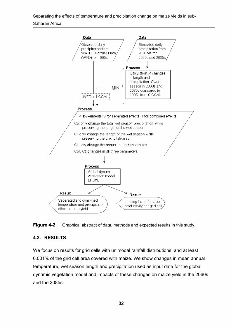
Separating the effects of temperature and precipitation change on maize yields in sub-
Saharan Africa
Figure 4-2 Graphical abstract of data, methods and expected results in this study.
4.3. RESULTS
We focus on results for grid cells with unimodal rainfall distributions, and at least
0.001% of the grid cell area covered with maize. We show changes in mean annual
temperature, wet season length and precipitation used as input data for the global
dynamic vegetation model and impacts of these changes on maize yield in the 2060s
and the 2085s.
82

Separating the effects of temperature and precipitation change on maize yields in sub-
Saharan Africa
Changes in temperature, wet season length and precipitation amount
GCM-projected daily precipitation data was analysed with regard to the largest
changes in the wet season precipitation and wet season length per grid cell after
removing the outliers. Note that these are stylized climate experiments combining
changes from different GCMs and using them as input for the global crop model. The
GCMs GFDL-CM2.1, GFDL-CM2.0 and CNRM-CM3 project the largest changes in
the wet season length and precipitation in many parts of SSA, therefore the stylized
climate experiments in almost half of the grid cells are based on climate change
projections from one of these models. In the second half climate data from the
remaining six GCMs is used in equal parts as input for the crop model. Most parts of
sub-Saharan Africa experience decreases in both variables of up to 20 % (Figure 4-
3). The wet season length and precipitation decrease most severely in parts of the
Sahel, Southern Africa and Central Africa. The spatial patterns of changes in
precipitation amount and length of the wet season are very similar in most parts.
However, in some regions the precipitation amount in the wet season decreases
more than the length of the wet season, like e.g. in West and East Africa between
5 °N and 18 °N. In contrast, the length of the wet season decreases more than the
wet season precipitation in parts of Tanzania, northern Mozambique, Ethiopia or
Angola. The wet season length and precipitation increase in 1.9-5.9 % of all grid cells
depending on the time period. Annual mean temperatures increase by 2-3 K in the
2060s and by 4-5 K in the 2085s whereas the increase is strongest in southern Africa
and in the Sahel (Figure 4-3).
83

Separating the effects of temperature and precipitation change on maize yields in sub-
Saharan Africa
Figure 4-3 Change in important agroclimatic variables according to GCM projections in
the 2060s (top) and 2085s (bottom) compared to the 1995s (from left to right): wet season
precipitation, wet season length and annual mean temperature. The largest changes in the
wet season per grid cell after removing the outliers and the corresponding temperatures are
shown. Dark violet colors in the leftmost and middle panel indicate a reduction of 50 % or
more.
Impacts on agricultural vegetation in sub-Saharan Africa
We compare simulations with the global dynamic vegetation model LPJmL driven by
the four climate experiments described in the methodology section in order to
estimate the impact of changes in wet season characteristics and in temperatures,
attributing the effects on crop productivity to these individual drivers.
84

Separating the effects of temperature and precipitation change on maize yields in sub-
Saharan Africa
Temperature increases lead to crop yield reductions in the 2060s in the maize-
growing regions of sub-Saharan Africa of 3-20 %, except for mountainous regions in
South and East Africa and parts of western Africa (Figure 4-4). In most regions maize
yields are lower in the 2085s than in the 2060s. The effect of reduced precipitation on
maize yields is even stronger in Southern Africa, southern parts of Mozambique and
Zambia, the Sahel and parts of Eastern Africa, with yield reductions of up to 30 %
and more. The effect of reduced precipitation in these regions clearly prevails over
the effect of increased temperatures in the 2060s and the 2085s. In all other parts,
e.g. in Central and Western Africa south of 13° N, the effect of increasing
temperature is limiting because of very slight yield changes due to changes in wet
season precipitation of -3 % to +3 %. In the mountainous regions of eastern and
southern Africa, increasing temperature leads to increasing crop productivity of up to
30 % and more, making reduced precipitation the only limiting effect. The reductions
in maize yields of 30 % and more in southern Africa result from very different
precipitation decreases of 50 % and more in southern Mozambique and Zimbabwe,
but only 10-20 % in South Africa (Figure 4-3). A shortening of the rainy season does
not affect maize yield negatively in most regions but partly leads to increasing crop
yields. Maize yields in central Africa with an already long rainy season (>200 days)
are not affected by a shortened wet season at all.
85
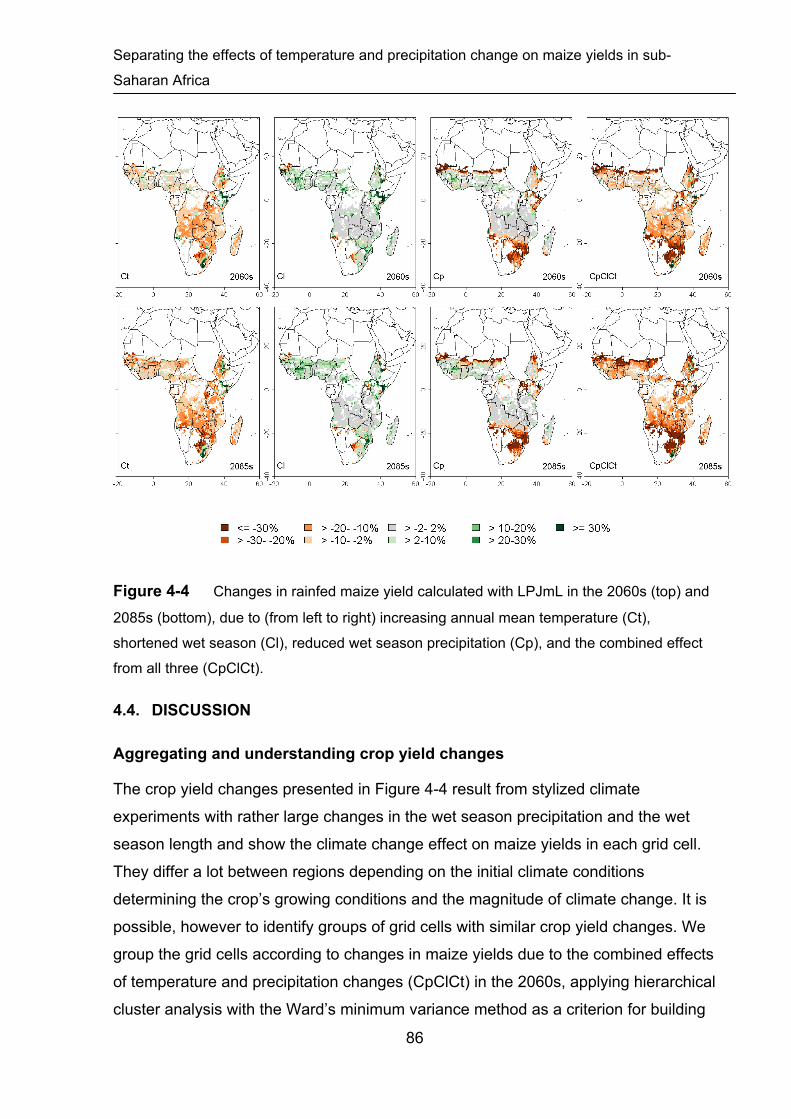
Separating the effects of temperature and precipitation change on maize yields in sub-
Saharan Africa
Figure 4-4 Changes in rainfed maize yield calculated with LPJmL in the 2060s (top) and
2085s (bottom), due to (from left to right) increasing annual mean temperature (Ct),
shortened wet season (Cl), reduced wet season precipitation (Cp), and the combined effect
from all three (CpClCt).
4.4. DISCUSSION
Aggregating and understanding crop yield changes
The crop yield changes presented in Figure 4-4 result from stylized climate
experiments with rather large changes in the wet season precipitation and the wet
season length and show the climate change effect on maize yields in each grid cell.
They differ a lot between regions depending on the initial climate conditions
determining the crop’s growing conditions and the magnitude of climate change. It is
possible, however to identify groups of grid cells with similar crop yield changes. We
group the grid cells according to changes in maize yields due to the combined effects
of temperature and precipitation changes (CpClCt) in the 2060s, applying hierarchical
cluster analysis with the Ward’s minimum variance method as a criterion for building
86

Separating the effects of temperature and precipitation change on maize yields in sub-
Saharan Africa
clusters with the R function hclust (Murtagh, 1985). The distance between 1-
dimensional clusters is calculated as the Euclidean distance. Each cluster differs in
the future crop yield changes (Figure 4-6) which indicate a high or low susceptibility
to climate change. The initial climatic conditions in the baseline climate in each
cluster might be different among the clusters as well (Figure 4-5, right side), as final
crop yields depend not only on the magnitude of climate change but also on the initial
climate conditions determining the crop’s growing conditions.
Figure 4-5 Distribution and characteristics of four groups resulting from hierarchical
cluster analyses of yield changes in the 2060s (Figure 4-4, panel top right). The stacked bar
plots on the right side show the probability that grid cells within a group belong to a certain
temperature class, wet season length class and wet season precipitation class. Labels at the
x-axis are the lower class limits.
Grid cells attributed to group A are located in the Sahel, in southern Africa and in
parts of Eastern Africa. The group is very susceptible to climate change with large
maize yield decreases of at least 33 % (Figure 4-6). Mean annual temperature in the
87

Separating the effects of temperature and precipitation change on maize yields in sub-
Saharan Africa
baseline climate is mostly above 28 °C, the wet season length is below 120 days and
the wet season precipitation is below 500 mm (Figure 4-5, right side). High mean
annual temperatures in the baseline climate and temperature increases of 2-3 K until
2060 indicate an increasing risk of extreme daily temperatures in group A. However,
according to our results a reduction in the wet season precipitation causes a stronger
decrease in crop yields than increasing temperatures in nearly all grid cells assigned
to this group (Figure 4-6). The growing conditions in this group are unfavourable for
growing crops already today but temperatures far beyond the temperature optimum
for photosynthesis (21-26 °C) do not damage the crop additionally in the model,
leading to a weak temperature effect compared to the precipitation effect.
Group B and group C are moderately to slightly susceptible to climate change with
maize yield changes between -33 % to -10 % and -10 % to +6 %, respectively
(Figure 4-5). Parts of Western Africa south of 13° N and of Central and East Africa
are belonging to group C, which is characterized by high annual mean temperature
(24-28 °C) and sufficient amounts of precipitation in the wet season (>750 mm). In
most grid cells belonging to group B or C the growing season is long and wet enough
for growing maize in a single cropping system so the length of the wet season does
not determine the magnitude of yield changes. For the same reason the effect of a
reduced wet season precipitation is less strong than the effect of increasing
temperatures (Figure 4-6). Temperatures increase are slightly stronger in parts of
southern Africa belonging to group B (Figure 4-3) leading to a stronger temperature
effect on maize yields than that in group C. A shorter wet season (Cl) only has a
marginal effect on maize yields in group B and C as the growing conditions are not
necessarily affected if the crop reaches maturity before the end of the wet season.
Group D is the smallest group and not susceptible to climate change at all. Maize
yield increases by at least 6 % (Figure 4-6) because increasing temperatures are
favourable in an environment with an annual mean temperature between 13 °C and
15 °C and a long wet season (Figure 4-5, right side). As also the mean rainfall per
rain day is increased in the Cl experiment with a shortened wet season, the growing
conditions improve leading to increasing maize yields in some regions i.e. many grid
cells in group D.
88

Separating the effects of temperature and precipitation change on maize yields in sub-
Saharan Africa
Figure 4-6 Crop yield changes in the 2060s from the combined (CpClCt) and separated
effects of changing temperature (Ct) and wet seasons (Cp, Cl) in groups shown in Figure 4-
5. Extreme data points that deviate from the borders of the box (Q25-Q75) by more than 1.5
times the interquartile range are not shown.
In group A-C with slight to large reductions in maize yields, the limiting effect in each
grid cell also determines the direction of yield change if all three effects are combined
and negative effects from increasing temperature and changing precipitation
exacerbate each other (Figure 4-4 for e.g. Zimbabwe, southern Mali or Burkina
Faso). In group D, in contrast the combined effect of changing temperatures and
precipitation is positive following mostly from the beneficial effect of increasing
temperatures.
Even slight to moderate yield changes might seriously endanger local food security if
food production is already instable or crop productivity is at a low level. The maize
yields in all four groups range between 0.65 t/ha and 2.6 t/ha (Q5-Q95) and are
89

Separating the effects of temperature and precipitation change on maize yields in sub-
Saharan Africa
evenly distributed over the groups therefore similar yield changes will have a very
different effect on local food security. This becomes evident when comparing yield
changes with an indicator of food security like the number of people undernourished
in a country (FAO, 2011b). Most parts of e.g. the Central African Republic are
belonging to group B with only slight yield changes but 40 % of the population was
undernourished in 2006-2008 making the country much more vulnerable to yield
reductions compared to Uganda with most parts of the country indeed belonging to
group C with higher yield decreases but less people undernourished today (22 %).
Uncertainty in GCM projections of precipitation
Although GCM projections agree on the level of median temperature increase, they
project very different precipitation patterns in various regions of sub-Saharan Africa
due to a large variety of model setting caused by the models’ resolution and model
physics, affecting e.g. the occurrence of convection or the vertical transport of
moisture in the tropics (Lin, 2007). This influences the distribution of wet and dry days
and the precipitation amount per wet day simulated in each GCM and in turn the
severity of water stress in the growing season. There is some consistency between
GCMs with respect to the projected increase of annual precipitation amount in East
Africa and a drying in southern Africa. A consistent increase in the number of
extremely wet seasons in West Africa and East Africa by 20 % and an increase of
extremely dry seasons by 20 % in southern Africa combined with an increase in the
rainfall intensity is also expected (Christensen et al., 2007). Most of the GCMs project
excessive precipitation over much of the tropics and, associated with that, insufficient
precipitation over much of the Equatorial Pacific (Lin, 2007). This double-ITCZ (Inter-
Tropical Convergence Zone) problem together with another common bias of GCMs,
the too strong persistence of tropical precipitation (Lin et al., 2006), might lead to
poor representation of tropical precipitation patterns in some GCMs. An important
element of tropical intra-seasonal variability and thus weather and climate forecasting
between 15° N and 15° S, the Madden–Julian oscillation, is simulated nearly realistic
from ECHAM5/MPI-OM and CNRM-CM3 (Lin et al., 2006). These models were
chosen for our study as well and provide the climate input data in 26% of all grid cells
in the studied region.
90

Separating the effects of temperature and precipitation change on maize yields in sub-
Saharan Africa
Limitations of modeling stress on crop growth and development
The global dynamic vegetation model LPJmL considers the effects of water stress on
crop growth and development and temperature effects on the photosynthesis rate
and length of the growing period (as described in the section “Modelling the impact
on agricultural vegetation”). Results from previous studies on heat stress effects on
crop yields in sub-Saharan Africa indicate that the Sahel and southeastern Africa are
most affected by heat stress (Teixeira et al., in press) and that maize yields are
negatively affected in areas with an annual mean temperature above 25 °C because
daily temperatures commonly exceed 30 °C. A yield loss of 10 % per one °C of
warming is possible in these regions (Lobell et al., 2011). These results agree well
with the large yield reductions of at least 33% in grid cells in the Sahel and parts of
Southern Africa assigned to group A with an annual mean temperature above 28 °C
and temperature increases of 2-3 °C in the 2060s. It is however not clear to what
extent maize yield is reduced because of shortened development phases, leading to
reduced light interception in an accelerated life cycle and because of a limited
photosynthesis rate. This study does not consider several damaging effects of heat
and water stress; on the other hand, the plants´ ability to develop heat and
desiccation tolerance is also omitted. The study of Barnabas et al. (2008) gives an
overview of these damaging effects which are also important for the growth and
development of cereals but not considered in the model. Among the most important
effects are oxidative damage, modifications in membrane functions, denaturation of
existing proteins, reductions in pollen germination ability due to high temperatures
(>30 °C) and the delay or even depression of flowering due to limited water supply.
For maize, daily temperatures above 33.5 °C and 38 °C were shown to reduce the
kernel growth rate and the pollen germination ability, respectively (Barnabas et al.,
2008).
The beneficial effect of elevated CO2 concentrations on plant growth and above-
ground biomass can be computed with LPJmL. This effect is not considered in the
study, as its effectiveness is questionable for maize without large additional nitrogen
inputs (Long et al., 2006). The risk of crop damage due to increased temperature or
water stress does not only depend on the magnitude of temperature and precipitation
changes but also on the vulnerability of a region to these changes determined by
91

Separating the effects of temperature and precipitation change on maize yields in sub-
Saharan Africa
current climatic conditions and farmer’s management strategies for adaptation such
as choosing an adapted sowing date or cropping system (Chapter 3). Selecting heat-
resistant crop varieties is another adaptation option helping to reduce negative
climate change impacts considerably e.g. in Mali, Butt et al. (2005) showed that heat-
resistant maize varieties simulated with EPIC are less affected from climate change
i.e. yields are reduced by 8.6 % compared to a reduction of 11.2 % without
adaptation for HadCM3. Also applying water-harvesting techniques (Rost et al.,
2009) and increasing rainwater productivity through conservation farming strategies
(Rockström et al., 2009) might lower the damage on crop yield considerably and are
sometimes very cost-effective at the same time (Ebi et al., 2011).
4.5. SUMMARY AND CONCLUSIONS
We show that the importance of the agro-climatic variables temperature, wet season
precipitation and wet season length for maize growth, varies in space depending on
the initial climate conditions and the magnitude of climate change. Crop yields
change considerably in regions with unsuitable or extreme growing conditions which
are very susceptible to even slight climate change and in regions which are exposed
to strong temperature and precipitation changes. The regions most vulnerable to
temperature increases are southern Africa and parts of East and West Africa with
annual mean temperatures of 18-24 °C which are exposed to annual temperature
increases of 2-3 K leading to maize yield decreases of more than 20 %. Parts of
South Africa, Zimbabwe, Mozambique and the Sahel with higher annual mean
temperatures above 28 °C are exposed to extreme daily temperatures but the
temperature effect in the model is similar to the effect in regions with cooler
temperature. This indicates that in the model increasing temperatures only affect the
crop by shortening the growing season and limiting photosynthesis but that damage
from extreme daily temperatures above 30 °C is largely underestimated in the model.
The same regions are even more susceptible to precipitation changes as they have
short (< 120 days) and dry (< 500 mm) growing seasons and reduced wet season
precipitation leads to maize yield reductions of 30 % and more. In the mountainous
regions of South Africa and East Africa temperature increases are beneficial for
maize growth and lead to increasing crop yields of up to 20-30 %. These findings
should be considered in drought and heat stress breeding programmes and in
92

Separating the effects of temperature and precipitation change on maize yields in sub-
Saharan Africa
studies on adaptation to climate change impacts. With climate change both,
temperature and precipitation will change but determining the limiting effect helps to
prioritize future research needs and to identify adequate crop varieties and
adaptation options in different environments.
The model is sensitive to all three agro-climatic variables wet season length, wet
season precipitation and temperature but reductions of crop yields mostly arise from
changes in temperature and wet season precipitation. A shortened wet season does
not affect maize growth in most parts of sub-Saharan Africa as maize is simulated to
grow at the beginning of the wet season and mostly reaches maturity before the end
of the wet season. Only in small parts of southern Africa and the Sahel with a wet
season length not exceeding 100 days, maize yields are reduced because of a
shortened wet season. The effect of a reduced wet season length would be much
stronger in multiple cropping regions where the second crop is at higher risk to be
influenced negatively from a shorter wet season. However, African farmers which
tend to be risk-averse will rather avoid a second cropping cycle that coincides with
the end of the wet season.
4.6. ACKNOWLEDGEMENTS
We acknowledge the modeling groups, the Program for Climate Model Diagnosis and
Intercomparison (PCMDI) and the WCRP's Working Group on Coupled Modelling
(WGCM) for their roles in making available the WCRP CMIP3 multi-model dataset.
Support of this dataset is provided by the Office of Science, U.S. Department of
Energy. We thank Sebastian Ostberg and Jens Heinke for preparing the LPJmL input
data on temperature and cloudiness and Jens Heinke for providing the WATCH
forcing data. We are also grateful to Jan Philipp Dietrich for his comments on the
scenario setting and the discussion of the results.
4.7. AUTHORS´ CONTRIBUTION
The contribution of the different authors was as follows: K.W. and C.M. conceived the
original idea of studying the effects of changing precipitation variability on crops. K.W.
expanded this into a study on separating the effects of temperature and precipitation
on crops. C.M. prepared the daily precipitation files from 18 GCMs, which was the
93

Separating the effects of temperature and precipitation change on maize yields in sub-
Saharan Africa
94
basis for analysing changes in the wet season length and precipitation. All authors
were involved in developing and discussing the methodology. K.W. prepared the
precipitation input files, did the model runs, prepared the figures, did literature
research and wrote the manuscript. All authors were involved in discussing the
results and reviewing the manuscript several times.

5. General Conclusions
In this chapter I first briefly summarize the key results and conclusions related to the
objectives of this thesis presented in the introduction. In addition, I recommend future
research needs which arise from the findings presented in the main chapters and
from my experience of modeling climate change impacts.
5.1. KEY RESULTS AND CONCLUSIONS
Agricultural crops are projected to be severely impacted by climate change in many
parts of sub-Saharan Africa, depending on the (i) magnitude of climate change and
(ii) depending on the crop, the cropping system and the adaptive capacity of farmers
in a region. The most important results from chapter 3 and 4 on the impacts of
climate change on agricultural crops and their determining factors are:
1. The aggregated crop yields in sub-Saharan Africa are projected to decline by 6-
24 % in the 2085s depending on the climate scenario, cropping system and
adaptation options.
2. Analysing the effects of changes in individual agroclimatic variables separately
makes it possible to understand their regional importance for overall crop yield
changes and to identify the limiting effect for food production in each region
3. Southern Africa is clearly the region most susceptible to climate change,
especially to precipitation changes, but also the region with the largest variability
in crop yield changes.
4. The Sahel north of 13° N and parts of Eastern Africa with short growing seasons
below 120 days and limited wet season precipitation of less than 500 mm are also
vulnerable to precipitation changes.
5. In most parts of Central and East Africa with longer growing seasons, in contrast,
the effect of temperature increase on crops overbalances the precipitation effect
and is most pronounced in a band stretching from Angola to Ethiopia in the
2060s. With even stronger temperature increases until the 2085s parts of Western
Africa south of 13° N are also impacted stronger.
95

General Conclusions
96
By applying certain management strategies for adaptation, farmers are potentially
able to reduce the negative effects of climate change on crops and minimize the risk
of crop failure by applying low-tech adaptation strategies. The most important results
from chapter 2 and 3 show the potential of management strategies for adaptation the
farmers might benefit from.
1. Crop yields are simulated to be higher and therefore food production in sub-
Saharan Africa would be less susceptible to climate change if the crop’s sowing
date is adapted to shifts of the rainy season. This is already an effective
adaptation option to current climate variability (+°6-8 %), but it becomes even
more important under climate change (+ 11-17 %). Sowing dates for global crop
models can be satisfactorily estimated from climate conditions with only one
month deviation to observed sowing dates in most of the locations but with some
uncertainty for tropical systems with high cropping intensities. The proposed
method therefore is suitable for global crop models and for climate change
assessment studies which should consider this management option.
2. Crop yields are simulated to be higher also if a second crop cultivar in a
sequential cropping system can be cultivated (+ 67-77 %) in regions with a long
growing season and if farmers have sufficient input and labour available for a
second cropping cycle. As a precondition for achieving this result I show the
distribution of the most important multiple cropping systems in ten African
countries and give evidence that farmers prefer to grow short-growing crop
cultivars in these systems in order to reduce the risk of crop failure.
3. Choosing the highest-yielding cropping system might lower negative climate
change impacts as well (+ 24-29 %). As this beneficial system might be an
uncommon or even unknown cropping system in a region and not necessarily the
traditional cropping system, its application might be limited. Also farmer decide on
the crops and cropping systems according to local biophysical or socio-economic
conditions which are not considered here.
Not only in sub-Saharan Africa but also on a global scale these management
strategies have the potential to increase the crop production in the same range as
water management strategies. Rost et al. (2009) showed the global potential of two

General Conclusions
97
water management strategies like collecting rainwater in cisterns, ponds or small
dams (“rainwater harvesting”) or soil and water conservation methods which increase
the water availability for plants (“vapour shift”). Applying these management
strategies globally would increase crop production by more than 50 % under the
present climate (Rost et al., 2009), and by more than 30 % under changing climate in
the most optimistic scenario (Figure 5-1). This is a theoretical potential of soil and
water conservation methods increasing the transpiration-to-evaporation ratio to 85 %.
In a moderate scenario, water management strategies increase crop production by 4-
13 % which is comparable to 6-12 % increases for sowing date and cropping system
adaptation and both are close to the achievable production increase from irrigation
(Figure 5-1). Assuming that in sub-Saharan Africa and other developing regions the
water management strategies are least efficient, crop production would still increase
by 1.5-4.6 % (Figure 5-1).
Figure 5-1 Achievable increases in global crop production (%) through different water
management and cropping system management strategies under climate change in the
2055s as compared to the current state: I Irrigation, SD adapted sowing dates, CS adapted
cropping system, SD+CD sowing dates and cropping system adaptation, VS Vapor shift with
different efficiency levels (10-85 % increase in plant transpiration), RH rainwater harvesting
with different efficiency levels (10-85 % rainwater stored), VS+RH Vapor shift and rainwater
harvesting with different efficiency levels (Rost et al., 2009; Waha et al., 2011).

General Conclusions
98
5.2. FUTURE RESEARCH PRIORITIES
From the results and conclusions of this thesis it is possible to continue with several
next steps and I consider three topics to be the most important future research
needs.
Up-scaling multiple cropping data to global scale
As I showed in chapter 3, multiple cropping is a common and widespread
management strategy to increase crop production, to lower the risk of total crop
failure and to minimize the negative effects of climate change in some regions.
Considering multiple cropping also in global studies about climate change impacts on
agriculture would enhance the reliability of these results considerably as adapting the
cropping system might be a suitable adaptation option in other world regions as well.
The first step would be to prepare a global land use dataset including multiple
cropping systems and fallow land, which is not available yet. Global land use data
sets (e.g. Portmann et al., 2010) can be combined with available regional datasets on
multiple cropping zones in India (Frolking et al., 2006), China (Frolking et al., 2002) or
Africa (chapter 3) and related data on e.g. farming and livelihood systems in Africa
(Thornton et al., 2006) or cropping calendars in Africa (FAO, 2010), which are based
on satellite data or agricultural surveys. This is a demanding task already, as the
different datasets will probably disagree in some regions. If information on existing
multiple cropping systems is still missing, the farmers choice of crops and cropping
systems can also be modeled as a function of climate conditions, soil properties,
expected profit and household characteristics (Kurukulasuriya & Mendelsohn, 2006;
Seo & Mendelsohn, 2008), considering that in developing countries farmers might
give a higher priority to stable food supply than to high profit. Secondly, model
parameters for a global application need adjustment as shown in chapter 3.2 for
Africa in order to represent shorter cropping cycles in a multiple cropping system.
Farmers clearly prefer long-growing crop cultivars in single cropping systems and
short-growing crop cultivars in sequential cropping systems.
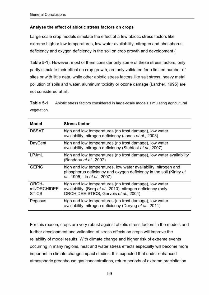
General Conclusions
99
Analyse the effect of abiotic stress factors on crops
Large-scale crop models simulate the effect of a few abiotic stress factors like
extreme high or low temperatures, low water availability, nitrogen and phosphorus
deficiency and oxygen deficiency in the soil on crop growth and development (
Table 5-1). However, most of them consider only some of these stress factors, only
partly simulate their effect on crop growth, are only validated for a limited number of
sites or with little data, while other abiotic stress factors like salt stress, heavy metal
pollution of soils and water, aluminum toxicity or ozone damage (Larcher, 1995) are
not considered at all.
Table 5-1 Abiotic stress factors considered in large-scale models simulating agricultural
vegetation.
Model Stress factor
DSSAT high and low temperatures (no frost damage), low water availability, nitrogen deficiency (Jones et al., 2003)
DayCent high and low temperatures (no frost damage), low water availability, nitrogen deficiency (Stehfest et al., 2007)
LPJmL high and low temperatures (no frost damage), low water availability (Bondeau et al., 2007)
GEPIC high and low temperatures, low water availability, nitrogen and phosphorus deficiency and oxygen deficiency in the soil (Kiniry et al., 1995; Liu et al., 2007)
ORCH-mil/ORCHIDEE-STICS
high and low temperatures (no frost damage), low water availability, (Berg et al., 2010), nitrogen deficiency (only ORCHIDEE-STICS, Gervois et al., 2004)
Pegasus high and low temperatures (no frost damage), low water availability, nitrogen deficiency (Deryng et al., 2011)
For this reason, crops are very robust against abiotic stress factors in the models and
further development and validation of stress effects on crops will improve the
reliability of model results. With climate change and higher risk of extreme events
occurring in many regions, heat and water stress effects especially will become more
important in climate change impact studies. It is expected that under enhanced
atmospheric greenhouse gas concentrations, return periods of extreme precipitation

General Conclusions
100
events will become shorter while precipitation intensity and the number of wet spells
as well as the frequency of high temperatures will increase in most areas (McGuffie
et al., 1999). I already showed the effect of high temperatures and low wet season
precipitation and their regional importance in chapter 4. These results should also be
discussed in the light of additional stress factors and the potentially beneficial CO2
fertilization effect, preferably for different crops, crop varieties and management
treatments. Field trial data from the CGIAR centers on agricultural research are most
suitable for this purpose, e.g. for tropical maize from 123 African research stations,
four crop varieties and five management regimes managed from the International
Maize and Wheat Improvement Center (CIMMYT) and others, which is available for
the period 1999 to 2007 (Bänziger et al., 2006; Lobell et al., 2011). Another source of
crop yield data under different management is the household survey used in chapter
3 containing more than 8600 households in ten African countries (Dinar et al., 2008)
and agricultural census data for individual countries, e.g. for Uganda (Fermont &
Benson, 2011). Building a database combining these data will be a first important
step.
Bridging the gap between model scales
Farmers decide on the best management strategy depending on local environmental
and economic conditions and accordingly act on a local scale, while large-scale crop
models like LPJmL focus on global or regional dynamics. In a decision making
process on how to develop the agricultural sector also under climate change a study
at a large scale can only be a first step for understanding the long-term and large-
scale limitations for agriculture in a region. To serve as a decision support tool on a
local scale a crop model needs to be adjusted to local soil and climate conditions and
validated using local agricultural data. Combining regional and global crop models
might be an option for bridging a gap between the two scales. Field or point models
suitable for simulating crop growth at a local scale often include a wide range of
management options and crop cultivars but require a lot of local knowledge and
parameters which are mostly not available on the global scale. Crop models on a
local scale can however provide knowledge about the most important drivers of crop
response to changing climate and improve model parameters considerably. These
findings then need to be assigned to a larger scale by e.g. assuming similar
limitations and processes in locations with similar growing conditions. This will be the

General Conclusions
101
most challenging part but a hierarchical cluster analysis to group individual points to
regions with similar crop response to climate seems to be a promising approach for
this. Several crop models were already applied in simulation studies in the tropics on
a local scale like e.g. APSIM (Keating et al., 2003), CropSyst (Stöckle et al., 1994),
GLAM (Challinor et al., 2005), RIDEV (Dingkuhn et al., 1995), SARRA-H (Dingkuhn
et al., 2003), STICS (Brisson et al., 2003).
From the results of my thesis I also conclude, that the following needs to be
considered in climate change impact studies by all means:
The context of food (in)security: In order to report on the progress made towards
achieving the World Development Goal of reducing the number of undernourished
people by half by the year 2015, the FAO started to publish the series “The state of
food insecurity in the world” in 1999. Countless governmental and non-governmental
organizations are engaged in monitoring and analysing the situation of countries and
people facing a high risk of undernourishment and hunger, which is largely a political
and economical problem. In addition to the main drivers of food insecurity, weak
governments, insufficient investment in agricultural technology, economic crises,
missing safety nets and social programmes and violent conflicts, to name but a few,
climate change poses a risk to vulnerable societies and the agricultural sector. It
therefore becomes part of the complex problem to achieve food security and develop
the agricultural sector making it a highly relevant topic connected to political and
economical topics. This requires good communication of the key results, limitations
and conclusions of a climate change impact study on agriculture to stakeholders.
Data quality and availability: The most important input data for a global model
simulating agricultural crops are climate data, soil data and data on land use und
management intensity. Comparing the amount of land already cultivated to the
amount of land assessed as potentially cultivable land in sub-Saharan Africa
indicates that there is huge potential for cropland expansion into areas currently not
used (Fischer et al., 2011). However, the amount of cultivated land might be
underestimated and the land with potential for cultivation might be overestimated
considerably. The estimates of total cropland in sub-Saharan Africa in 1988/90
published in the FAO study “World agriculture towards 2010” needed adjustments of
51 % and estimates on the proportion of land cultivated in Africa still differ between

General Conclusions
102
different sources from 18% to 26% (Young, 1999). Reasons for this uncertainty in
cropland estimates are oversimplifications in global soil maps, the questionable
nature of land use statistics especially in developing countries and neglecting the
demand for land for non-agricultural purposes. Young (1999) therefore suggests that
“estimates of the total spare land in the developing world, and those for individual
countries, should be reduced to half or less the values given” (p.17). In order to
enhance the representation of agricultural area in global land use data sets,
MIRCA2000 (Portmann et al., 2010; Portmann et al., 2008) and SPAM2000 (You et
al., 2009) were developed recently. These two datasets are currently the most
comprehensive global datasets combining existing data with national and sub-
national agricultural statistics and surveys and both are accessible via their project
web pages. SPAM2000 reports crop area and production on a sub-national level and
also distinguishes between three levels of input systems: irrigated, rainfed high-
input/commercial, and rainfed low-input/subsistence. MIRCA2000 also distinguishes
between rainfed and irrigated crop area and additional reports crop calendars for 26
crops. Both datasets are the most comprehensive global datasets on cropland
distribution at the moment.
Presentation and aggregation of model results: The magnitude of crop yield changes
reported in climate change impact studies depends on the aggregation level, as
negative climate change effects might be counterbalanced by positive effects if the
aggregation units are too heterogeneous and extremes are not visible anymore. On
the other hand it is important to aggregate results for comparisons between
countries, world regions and time periods. Cluster analyses might be an appropriate
tool for finding homogenous units as proposed for regional climate change results
(Mahlstein & Knutti, 2010), global-land use patterns (Dietrich, 2011) and crop yield
changes due to climate change in this thesis (chapter 4).

Summary
Agriculture is one of the most important human activities providing food and more
agricultural goods for seven billion people around the world and is of special
importance in sub-Saharan Africa. The majority of people depends on the agricultural
sector for their livelihoods and will suffer from negative climate change impacts on
agriculture until the middle and end of the 21st century, even more if weak
governments, economic crises or violent conflicts endanger the countries’ food
security. The impact of temperature increases and changing precipitation patterns on
agricultural vegetation motivated this thesis in the first place. Analysing the potentials
of reducing negative climate change impacts by adapting crop management to
changing climate is a second objective of the thesis.
As a precondition for simulating climate change impacts on agricultural crops with a
global crop model first the timing of sowing in the tropics was improved and validated
as this is an important factor determining the length and timing of the crops´
development phases, the occurrence of water stress and final crop yield. Crop yields
are projected to decline in most regions which is evident from the results of this
thesis, but the uncertainties that exist in climate projections and in the efficiency of
adaptation options because of political, economical or institutional obstacles have to
be considered. The effect of temperature increases and changing precipitation
patterns on crop yields can be analyzed separately and varies in space across the
continent. Southern Africa is clearly the region most susceptible to climate change,
especially to precipitation changes. The Sahel north of 13° N and parts of Eastern
Africa with short growing seasons below 120 days and limited wet season
precipitation of less than 500 mm are also vulnerable to precipitation changes while
in most other part of East and Central Africa, in contrast, the effect of temperature
increase on crops overbalances the precipitation effect and is most pronounced in a
band stretching from Angola to Ethiopia in the 2060s.
The results of this thesis confirm the findings from previous studies on the magnitude
of climate change impact on crops in sub-Saharan Africa but beyond that helps to
understand the drivers of these changes and the potential of certain management
strategies for adaptation in more detail. Crop yield changes depend on the initial
103

Summary
104
growing conditions, on the magnitude of climate change, and on the crop, cropping
system and adaptive capacity of African farmers which is only now evident from this
comprehensive study for sub-Saharan Africa. Furthermore this study improves the
representation of tropical cropping systems in a global crop model and considers the
major food crops cultivated in sub-Saharan Africa and climate change impacts
throughout the continent.

Appendices
A ANALYSIS OF SOWING DATE PATTERNS OF ELEVEN CROPS
For each crop three maps show the a) difference between simulated sowing dates
and observed sowing dates, b) simulated sowing date, c) observed sowing dates
according to MIRCA 2000 (Portmann et al., 2008). White colours indicate crop area
smaller than 0.001 % of grid cell area. Sowing dates in regions without seasonality
are not shown.
105

Appendix A
Mollweide equal area projection
a)
b)
c)
0 2.500 5.000 7.500 10.000km
day of year1 - 3031 - 6061 - 9091 - 120
121 - 150151 - 180181 - 210211 - 240241 - 270271 - 300301 - 330
331 - 365
day of year1 - 3031 - 6061 - 9091 - 120
121 - 150151 - 180181 - 210211 - 240241 - 270271 - 300301 - 330
331 - 365
months-6-5-4
-3-2-10123
456
Figure A-1 Analysis of sowing date patterns of wheat.
106

Appendix A
Mollweide equal area projection
a)
b)
c)
0 2.500 5.000 7.500 10.000km
day of year1 - 3031 - 6061 - 9091 - 120
121 - 150151 - 180181 - 210211 - 240241 - 270271 - 300301 - 330
331 - 365
day of year1 - 3031 - 6061 - 9091 - 120
121 - 150151 - 180181 - 210211 - 240241 - 270271 - 300301 - 330
331 - 365
months-6-5-4
-3-2-10123
456
Figure A-2 Analysis of sowing date patterns of rice.
107

Appendix A
Mollweide equal area projection
a)
b)
c)
0 2.500 5.000 7.500 10.000km
day of year1 - 3031 - 6061 - 9091 - 120
121 - 150151 - 180181 - 210211 - 240241 - 270271 - 300301 - 330
331 - 365
day of year1 - 3031 - 6061 - 9091 - 120
121 - 150151 - 180181 - 210211 - 240241 - 270271 - 300301 - 330
331 - 365
months-6-5-4
-3-2-10123
456
Figure A-3 Analysis of sowing date patterns of maize.
108

Appendix A
Mollweide equal area projection
a)
b)
c)
0 2.500 5.000 7.500 10.000km
day of year1 - 3031 - 6061 - 9091 - 120
121 - 150151 - 180181 - 210211 - 240241 - 270271 - 300301 - 330
331 - 365
day of year1 - 3031 - 6061 - 9091 - 120
121 - 150151 - 180181 - 210211 - 240241 - 270271 - 300301 - 330
331 - 365
months-6-5-4
-3-2-10123
456
Figure A-4 Analysis of sowing date patterns of millet.
109

Appendix A
Mollweide equal area projection
a)
b)
c)
0 2.500 5.000 7.500 10.000km
day of year1 - 3031 - 6061 - 9091 - 120
121 - 150151 - 180181 - 210211 - 240241 - 270271 - 300301 - 330
331 - 365
day of year1 - 3031 - 6061 - 9091 - 120
121 - 150151 - 180181 - 210211 - 240241 - 270271 - 300301 - 330
331 - 365
months-6-5-4
-3-2-10123
456
Figure A-5 Analysis of sowing date patterns of pulses.
110

Appendix A
Mollweide equal area projection
a)
b)
c)
0 2.500 5.000 7.500 10.000km
day of year1 - 3031 - 6061 - 9091 - 120
121 - 150151 - 180181 - 210211 - 240241 - 270271 - 300301 - 330
331 - 365
day of year1 - 3031 - 6061 - 9091 - 120
121 - 150151 - 180181 - 210211 - 240241 - 270271 - 300301 - 330
331 - 365
months-6-5-4
-3-2-10123
456
Figure A-6 Analysis of sowing date patterns of sugar beet.
111

Appendix A
Mollweide equal area projection
a)
b)
c)
0 2.500 5.000 7.500 10.000km
day of year1 - 3031 - 6061 - 9091 - 120
121 - 150151 - 180181 - 210211 - 240241 - 270271 - 300301 - 330
331 - 365
day of year1 - 3031 - 6061 - 9091 - 120
121 - 150151 - 180181 - 210211 - 240241 - 270271 - 300301 - 330
331 - 365
months-6-5-4
-3-2-10123
456
Figure A-7 Analysis of sowing date patterns of cassava.
112

Appendix A
Mollweide equal area projection
a)
b)
c)
0 2.500 5.000 7.500 10.000km
day of year1 - 3031 - 6061 - 9091 - 120
121 - 150151 - 180181 - 210211 - 240241 - 270271 - 300301 - 330
331 - 365
day of year1 - 3031 - 6061 - 9091 - 120
121 - 150151 - 180181 - 210211 - 240241 - 270271 - 300301 - 330
331 - 365
months-6-5-4
-3-2-10123
456
Figure A-8 Analysis of sowing date patterns of sunflower.
113

Appendix A
Mollweide equal area projection
a)
b)
c)
0 2.500 5.000 7.500 10.000km
day of year1 - 3031 - 6061 - 9091 - 120
121 - 150151 - 180181 - 210211 - 240241 - 270271 - 300301 - 330
331 - 365
day of year1 - 3031 - 6061 - 9091 - 120
121 - 150151 - 180181 - 210211 - 240241 - 270271 - 300301 - 330
331 - 365
months-6-5-4
-3-2-10123
456
Figure A-9 Analysis of sowing date patterns of soybean.
114

Appendix A
Mollweide equal area projection
a)
b)
c)
0 2.500 5.000 7.500 10.000km
day of year1 - 3031 - 6061 - 9091 - 120
121 - 150151 - 180181 - 210211 - 240241 - 270271 - 300301 - 330
331 - 365
day of year1 - 3031 - 6061 - 9091 - 120
121 - 150151 - 180181 - 210211 - 240241 - 270271 - 300301 - 330
331 - 365
months-6-5-4
-3-2-10123
456
Figure A-10 Analysis of sowing date patterns of groundnut.
115

Appendix A
Mollweide equal area projection
a)
b)
c)
0 2.500 5.000 7.500 10.000km
day of year1 - 3031 - 6061 - 9091 - 120
121 - 150151 - 180181 - 210211 - 240241 - 270271 - 300301 - 330
331 - 365
day of year1 - 3031 - 6061 - 9091 - 120
121 - 150151 - 180181 - 210211 - 240241 - 270271 - 300301 - 330
331 - 365
months-6-5-4
-3-2-10123
456
Figure A-11 Analysis of sowing date patterns of rapeseed.
116

Appendix B
B SENSITIVITY ANALYSIS OF CROP YIELD ON SOWING DATE
Methodology
A possible application of sowing dates simulated with the presented methodology is
to provide global crop growth models under future conditions with suitable cropping
windows. We tested the sensitivity of the LPJmL dynamic global vegetation and crop
model for different sowing dates on simulated crop yields for five locations with
different seasonality types, using maize as an example crop.
In LPJmL, crop growth is simulated using a combination of processes
(photosynthesis, respiration, evapotranspiration, and leaf area development) on a
daily basis (for more details, see (Bondeau et al., 2007). LPJmL does not consider
the effects of extreme temperatures on crop growth and development, e.g. frost
damage. Phenological development of maize is simulated by accumulating
temperature above the maize-specific base temperature (8°C) until maturity is
reached, taking into account the effect of photoperiod, as applied in the
AFRCWHEAT2 model (Ewert et al., 1996), until anthesis. It was assumed for the five
locations that farmers grow cultivars which are adapted to their environment.
Required temperature sums till maturity per location-specific cultivar were calculated
based on observed sowing and harvest dates, monthly temperature data from the
year 1998, and photoperiods. Equal sensitivity to photoperiod between the cultivars
was assumed (the optimum photoperiod was assumed to be 12.5h and the base
photoperiod 24h). Yield was simulated for each location for a range of sowing dates
(52, starting at the first of January, with steps of 7 days) for rainfed conditions, using
the monthly climate data of the year 1998, and assuming that farmers grow the same
cultivar throughout the whole year. The crop was allowed to grow for a period of
maximum 250 days.
Results and Discussion
In Figure B-1, we display simulated maize yields per sowing date for the five
locations, compared to the maximum simulated maize yield per location.
117

Appendix B
Figure B-1 Sensitivity of maize yield to sowing dates for five locations. Between brackets,
the simulated respectively observed sowing dates are given. The dashed line indicates 80%
of maximum simulated yield.
The sensitivity of simulated maize yield to the sowing date at a location with no
seasonality (Iquitos, Peru) is relatively small: simulated yield is, irrespective of sowing
date, always at least 80% of the maximum simulated yield. Larger sensitivity is
shown for locations with temperature seasonality (Amsterdam, the Netherlands and
Kansas City, USA). In the Netherlands, yields of at least 80% of the maximum yield
are simulated, with sowing dates ranging from day of year 14 to day of year 140. In
the USA, yields of at least 80% of the maximum yield are simulated, with sowing
dates ranging from day of year 21 to day of year 147. In a location with precipitation
seasonality and a long wet season (Abuja, Nigeria), the range of sowing dates which
results in simulated yields of at least 80% of the maximum is wider in comparison to a
location with a shorter wet season (Delhi, India).
118

Appendix C
C WATER STRESS AFFECTING ROOT BIOMASS
Without water stress, root biomass decreases from 40 % at the beginning of the
phenological cycle to a minimum of 20 % of total biomass at maturity (Neitsch et al.,
2002) (Figure C-1 A).
With increasing water stress the fraction of total biomass allocated to the roots now
increases exponentially between that minimum and a maximum of 40 % of total
biomass (similar to the reduction in the harvest index with increasing water stress
described in (Neitsch et al., 2002)) in order to enhance water uptake from an
extensive root system during dry periods (Figure C-1 B).
As the above ground biomass thus more strongly responds to water stress, the
harvest index is no longer scaled by water stress as originally described by Bondeau
et al. (2007).
Figure C-1 Biomass fraction allocated to the roots as simulated in LPJmL, A: without
water stress as a function of phenological development, and B: depending on the water
stress factor at different phenological stages. A water stress factor of 0 indicates high water
stress
119

Appendix D
D COMPARISON OF THE START OF THE GROWING SEASON TO SATELLITE
DATA
We compare the start of the main rainy season simulated by LPJmL to the start of the
growing season obtained from MODIS satellite data providing the time of greening up
(Figure D-1) in order to validate the correct timing of a crop’s sowing date.
Figure D-1 Comparison of A: simulated and B: observed start of the growing season (in
weeks). Simulations were made with LPJmL and the observed start of the growing season is
derived from MODIS satellite data (HarvestChoice, 2010). White areas indicate no data.
The differences between the simulated and observed start of the growing season are
low with a mean error of 2 ¾ weeks, and a Willmott coefficient of agreement of 0.56.
There are considerably larger disagreements than 20 weeks in the mountainous
regions of Eastern Africa and desert regions of Namibia.
120

Appendix E
E MODEL’S ABILITY TO SIMULATE NATIONAL CROP YIELDS IN SUB-
SAHARAN AFRICA
To provide an assessment of the validness of crop yields simulated with LPJmL we
compare country-averaged yields from six crops used in this study in 48 countries of
sub-Saharan Africa for the five-year period from 1999 to 2003 to FAO yields in the
same period (FAO, 2011a). The annual fractional coverage of individual crop area
per grid cell is prescribed using a newly developed land-use dataset (Fader et al.,
2010). As a measure of agreement we calculate the Willmott coefficient of agreement
(W) (Willmott, 1982) and the Nash-Sutcliffe efficiency (EF) (Nash & Sutcliffe, 1970)
from the area-weighted deviations between simulated and observed yields:
where, is the simulated LPJmL and the observed FAO yield (t FM/ha) in a
country i, the mean observed FAO yield, the cultivated area (ha) of a crop in
country i, and N the number of countries. The Nash-Sutcliffe efficiency ranges from -
∞ to 1 (perfect fit), and the Willmott index of agreement ranges from 0 to 1 (perfect
fit).
As the rice yield in Somalia of 5.88 t/ha reported from FAO seems to be far too high
and is based on unofficial statistics, we used SPAM data (You & Wood, 2004; You et
al., 2010), which gives a rice yield of 1.85 t/ha for the year 2000 for comparison to
LPJmL rice yield. Figure E-1 to Figure E-6 show the comparison between LPJmL and
FAO yields for the six crops simulated in this study.
121

Appendix E
Figure E-1 Comparison of LPJmL and FAO cassava yields. Circle radius indicates the
size of total cropland under cassava in an individual country.
Figure E-2 Comparison of LPJmL and FAO cowpea yields. Circle radius indicates the
size of total cropland under cowpea in an individual country.
122

Appendix E
Figure E-3 Comparison of LPJmL and FAO groundnut yields. Circle radius indicates the
size of total cropland under groundnut in an individual country.
Figure E-4 Comparison of LPJmL and FAO maize yields. Circle radius indicates the size
of total cropland under maize in an individual country.
123

Appendix E
124
Figure E-5 Comparison of LPJmL and FAO rice yields. Circle radius indicates the size of
total cropland under rice in an individual country.
Figure E-6 Comparison of LPJmL and FAO wheat yields. Circle radius indicates the size
of total cropland under wheat in an individual country

F DETAILED LIST OF SIMULATED CROP YIELDS PER LOCATION
Table F-1 Overview of mean crop yields and crop yield changes per country and management scenario in 2070-2099 compared to 1971-
2000 averaged over three GCMs. Values are mean crop calorific yields in grid cells with a specific combination of a traditional sequential
cropping system (TS/TSco) and a highest-yielding sequential cropping system (HS/HSco).
Crop yield 1971-2000 [Mcal/ha] Crop yield 2070-2099 [Mcal/ha] Country and administrative unit
TSco TS SCco SC HSco HS TSco TS SCco SC HSco HS
Rice-Rice Rice Maize-Maize Rice-Rice Rice Maize-Maize
13666 18717 11204 10498 13666 18717 12222 12849 4769 4057 12222 12849 Bama
(-11%) (-31%) (-57%) (-61%) (-11%) (-31%) Rice-Maize Rice Maize-Maize Rice-Maize Rice Maize-Maize
7907 10135 2418 6105 16012 16196 5531 6521 479 2181 10939 12629
Bu
rkin
a F
aso
Tibele
(-30%) (-36%) (-80%) (-64%) (-32%) (-22%) Groundnut-Maize Groundnut Wheat-Maize Groundnut-Maize Groundnut Wheat-Maize
9668 9633 3218 3189 14247 14093 7989 8136 2360 2502 11475 12003 Sanaga Maritime, Wouri
(-17%) (-16%) (-27%) (-22%) (-19%) (-15%) Maize-Groundnut Maize Wheat-Maize Maize-Groundnut Maize Wheat-Maize
12210 12239 8671 8701 16388 16484 10090 10176 7757 7616 12947 13841 Mbam-et-Inoubou
(-17%) (-17%) (-11%) (-12%) (-21%) (-16%) Maize-Wheat Maize Maize-Wheat Maize-Wheat Maize Maize-Wheat
18120 19317 10977 11571 18120 19317 16356 17953 8909 9813 16356 17953 Vina
(-10%) (-7%) (-19%) (-15%) (-10%) (-7%) Groundnut-Maize Groundnut Maize-Wheat Groundnut-Maize Groundnut Maize-Wheat
9839 9906 3239 3270 14850 14802 7967 8233 2312 2535 12347 12652
Cam
ero
on
Moungo, Sanaga-Maritime
(-19%) (-17%) (-29%) (-22%) (-17%) (-15%)

Continuation Table F-1
Groundnut-Cassava Groundnut Maize-Wheat Groundnut-Cassava Groundnut Maize-Wheat
8496 8694 3557 3619 15944 15958 10127 8448 2528 2774 13208 13545 Momo
(19%) (-3%) (-29%) (-23%) (-17%) (-15%) Maize-Wheat Maize Maize-Maize Maize-Wheat Maize Maize-Maize
17808 18189 9736 10253 18937 19144 14243 15900 7887 8858 14956 16163 Vina
(-20%) (-13%) (-19%) (-14%) (-21%) (-16%) Maize-Maize Maize Maize-Maize Maize-Maize Maize Maize-Maize
16188 16729 9050 9349 16188 16729 13824 14384 7686 8103 13824 14384 Various (>3)
(-15%) (-14%) (-15%) (-13%) (-15%) (-14%) Cassava-Maize Cassava Maize-Maize Cassava-Maize Cassava Maize-Maize
11352 11355 10788 10984 14382 14193 10886 116501058
710329 12788 12410
Nyong-et-Kelle
(-4%) (3%) (-2%) (-6%) (-11%) (-13%) Cassava-Cowpea Cassava Maize-Maize Cassava-Cowpea Cassava Maize-Maize
11737 11741 10803 10787 14776 14825 11304 105721011
410283 12865 12729
Lekie
(-4%) (-10%) (-6%) (-5%) (-13%) (-14%) Groundnut-Maize Groundnut Maize-Maize Groundnut-Maize Groundnut Maize-Maize
8388 8797 3944 3932 14399 14412 6870 7806 2948 3103 12676 12715 Moungo, Ntem
(-18%) (-11%) (-25%) (-21%) (-12%) (-12%) Maize-Groundnut Maize Maize-Maize Maize-Groundnut Maize Maize-Maize
12291 12487 9055 9251 17016 17181 9824 10377 7931 8168 14045 14420 Mbam-et-Inoubou
(-20%) (-17%) (-12%) (-12%) (-17%) (-16%) Ground.-Ground. Groundnut Maize-Maize Ground.-Ground. Groundnut Maize-Maize
8263 8290 6501 6529 15094 15223 8301 8516 4039 4411 17384 16852 Bui
(0%) (3%) (-38%) (-32%) (15%) (11%) Groundnut-Maize Groundnut Cassava-Maize Groundnut-Maize Groundnut Cassava-Maize
7445 7362 2560 2590 11670 11715 4911 4420 1700 2036 10159 10170
Cam
ero
on
Manju
(-34%) (-40%) (-34%) (-21%) (-13%) (-13%)

Continuation Table F-1
Maize-Wheat Maize Cassava-Cowpea Maize-Wheat Maize Cassava-Cowpea
11659 12490 10212 10942 16854 18755 9542 10958 8214 9321 14539 17797
Eth
iop
ia
Kembata-Timbaro, Wolaita (-18%) (-12%) (-20%) (-15%) (-14%) (-5%)
Maize-Rice Maize Cassava-Cowpea Maize-Rice Maize Cassava-Cowpea
11840 12033 5554 5814 13458 13645 8155 9452 4329 4915 11524 11904 Nkwanta
(-31%) (-21%) (-22%) (-15%) (-14%) (-13%) Maize-Maize Maize Cassava-Cowpea Maize-Maize Maize Cassava-Cowpea
9794 10361 5212 5756 14449 14829 8008 8847 4077 4882 12040 12719 Various (>3)
(-18%) (-15%) (-22%) (-15%) (-17%) (-14%) Groundnut-Rice Groundnut Cassava-Cowpea Groundnut-Rice Groundnut Cassava-Cowpea
11210 11606 4681 5104 12368 12725 6181 7873 1948 3134 10432 10861 Tolon-Kumbungu
(-45%) (-32%) (-58%) (-39%) (-16%) (-15%) Groundnut-Maize Groundnut Cassava-Cowpea Groundnut-Maize Groundnut Cassava-Cowpea
10755 10328 5361 5243 12882 13536 7551 7575 3334 3398 11310 11840
Gh
ana
Sene
(-30%) (-27%) (-38%) (-35%) (-12%) (-13%) Maize-Maize Maize Wheat-Maize Maize-Maize Maize Wheat-Maize
4815 4847 5167 5170 10051 10601 8615 9614 7878 8115 15968 17462 Muranga, Nyeri, Embu
(79%) (98%) (52%) (57%) (59%) (65%) Maize-Maize Maize Rice-Rice Maize-Maize Maize Rice-Rice
5267 5339 5659 5685 9883 9870 8757 9292 8147 8481 15563 15945 Nyeri
(66%) (74%) (44%) (49%) (57%) (62%) Maize-Maize Maize Maize-Maize Maize-Maize Maize Maize-Maize
5986 8008 3123 4527 5986 8008 5006 7399 2678 4350 5006 7399 Kajiado, Kitui
(-16%) (-8%) (-14%) (-4%) (-16%) (-8%) Maize-Maize Maize Cassava-Maize Maize-Maize Maize Cassava-Maize
10038 10959 6325 7144 16262 17009 9929 11398 5205 6332 12330 15549
Ken
ya
Various (>3)
(-1%) (4%) (-18%) (-11%) (-24%) (-9%)

Continuation Table F-1
Maize-Groundnut Maize Cassava-Maize Maize-Groundnut Maize Cassava-Maize
16128 17086 6753 7546 22401 23206 10850 13313 5436 6780 15162 19433 Kakamenga
(-33%) (-22%) (-20%) (-10%) (-32%) (-16%) Maize-Maize Maize Cassava-Cowpea Maize-Maize Maize Cassava-Cowpea
7541 9497 4714 5885 12010 13991 6658 8831 3891 5154 9414 11822 Various (>3)
(-12%) (-7%) (-17%) (-12%) (-22%) (-15%) Maize-Groundnut Maize Cassava-Cowpea Maize-Groundnut Maize Cassava-Cowpea
9473 9862 9267 9784 27098 28204 16435 18003 7335 8172 23307 26014 Bungoma
(73%) (83%) (-21%) (-16%) (-14%) (-8%)
Maize-Maize Maize Cassava-Cowpea Maize-Maize Maize Cassava-Cowpea
5177 7501 4269 5708 7744 9118 4592 7497 3544 5049 3494 7026 Various (>3)
(-11%) (0%) (-17%) (-12%) (-55%) (-23%) Maize-Maize Maize Ground..-Ground. Maize-Maize Maize Ground..-Ground.
9666 9676 10376 10388 19512 19586 15287 14988 8776 8922 18422 16283
Ken
ya
Bomet
(58%) (55%) (-15%) (-14%) (-6%) (-17%) Wheat-Maize Wheat Wheat-Maize Wheat-Maize Wheat Wheat-Maize
15923 15888 12742 12831 15923 15888 15268 16875 7110 9341 15268 16875 Bethlehem, Lydenburg
(-4%) (6%) (-44%) (-27%) (-4%) (6%) Maize-Wheat Maize Wheat-Maize Maize-Wheat Maize Wheat-Maize
3446 3495 3664 3705 10581 10396 3961 4974 2550 4417 7011 3555 Aberden
(15%) (42%) (-30%) (19%) (-34%) (-66%) Wheat-Maize Wheat Maize-Wheat Wheat-Maize Wheat Maize-Wheat
8985 9802 8541 8283 15620 15660 14090 21531 3617 13177 17318 19634 Lydenburg
(57%) (120%) (-58%) (59%) (11%) (25%) Maize-Wheat Maize Cassava-Maize Maize-Wheat Maize Cassava-Maize
3978 3922 4300 4234 4199 4155 3792 3556 3839 3054 3872 3900 Aberden
(-5%) (-9%) (-11%) (-28%) (-8%) (-6%) Maize-Wheat Maize Cassava-Cowpea Maize-Wheat Maize Cassava-Cowpea
4827 4898 5124 4964 4900 5129 4987 4732 4580 3847 706 2703
So
uth
Afr
ica
Aberden
(3%) (-3%) (-11%) (-22%) (-86%) (-47%)

Continuation Table F-1
Maize-Wheat Maize Maize-Wheat Maize-Wheat Maize Maize-Wheat
13063 12505 4160 4179 15299 15931 9130 11357 1542 3082 3954 9161 Masvingo
(-30%) (-9%) (-63%) (-26%) (-74%) (-42%) Maize-Maize Maize Maize-Maize Maize-Maize Maize Maize-Maize
6042 7091 2966 3840 9791 14778 4256 5632 1527 2763 3857 8347 Zim
bab
we
Chegutu, Chipinge
(-30%) (-21%) (-49%) (-28%) (-61%) (-44%)

Appendix G
G GLOBAL CIRCULATION MODELS USED IN THIS STUDY
Table G-1 Global circulation models used in this study (Randall et al., 2007).
Model name Research Group(s) Country Available reporting periods
CGCM3.1(T47) Canadian Centre for Climate Modelling and Analysis
Canada 2046-2065, 2081-2100
CNRM-CM3 Météo-France / Centre National de Recherches Météorologiques
France 2046-2065, 2081-2100
CSIRO-Mk3.0 Commonwealth Scientific and Industrial Research Organisation, Atmospheric Research
Australia 2046-2065, 2081-2100
ECHAM5/MPI-OM Max Planck Institute for Meteorology
Germany 2046-2065, 2081-2100
GFDL-CM2.0 2046-2065, 2081-2100
U.S. Department of Commerce / National Oceanic and Atmospheric Administration / Geophysical Fluid Dynamics Laboratory
USA
GFDL-CM2.1 2046-2065, 2081-2100
IPSL-CM4 Institut Pierre Simon Laplace France 2046-2065, 2081-2100
MRI-CGCM2.3.2 Meteorological Research Institute
Japan 2046-2065, 2081-2100
PCM National Center for Atmospheric Research
USA 2046-2065, 2080-2099
The Coupled Model Intercomparison Project phase 3 (CMIP3) multi-model dataset contains more than these GCMs. For this study eight GCMs were excluded because the data was not complete and one GCM was excluded because data on the precipitation amount in the wet season deviates from the mean by more than three standard deviations.
130

Appendix H
H METHOD OF GENERATING STYLIZED PRECIPITATION SCENARIOS
Identifying the largest change in wet season characteristics
We first calculate the largest relative changes in total precipitation and length of the
wet season in combination for each grid cell after excluding all outliers that deviate
from the mean by more than two standard deviations to avoid overly emphasizing on
extremes. We do this for the two time periods 2060s and 2085s separately as
follows:
with n=9, where and are the precipitation in the wet season and length of the
wet season, respectively at time t and for GCM i, and the precipitation in
the wet season and length of the wet season in the 1995s and for GCM i.
tiP, tiL ,
1995,iP 1995,iL
We then assign the individual relative changes in both variables to the baseline
climate of the WATCH Forcing Data (WFD) to obtain the daily precipitation for the
climate experiments Cp, Cl and CpClCt described in the methods section. Figure H-1
shows an example for changes in daily precipitation in the 2060s for the GCM
ECHAM5.
131

Appendix H
Figure H-1 Daily precipitation changes in the 2060s for an example cell (Gambia:
Lat = 13° 25’ N, Lon = 16° 75’ W). Top: Daily precipitation in the 1995s from WATCH Forcing
Data (WFD) and projected changes in total precipitation and length of the wet season from
nine GCMs. Bottom: Daily precipitation in the 2060s in the three climate experiments CpClCt
(combined), Cp (Changed precipitation), and Cl (Changed length).
Overestimation of precipitation changes
It is assumed that assigning relative changes from GCM data to WATCH Forcing
Data (WFD) as a common baseline climate is an adequate procedure, as this data
lies within the range of baseline climates from all GCMs (Figure H-1). However, the
Kolmogorov–Smirnov test on the equality of distributions indicates that the total
precipitation and the length of the wet season in the 1995s calculated from GCMs
and from WFD differ significantly (p<0.001) (Figure H-1). Therefore, changes in the
132

Appendix H
2060s and the 2085s in total precipitation and length of the wet season may be
overestimated if GCMs significantly underestimate actual values (Füssel, 2003).
The test statistic of the Kolmogorov-Smirnov test D gives an indication of the
direction and strength of these differences. D is the maximum vertical deviation
between two cumulative distribution functions, i.e. for the comparison between WFD
and the GCM ECHAM5 with D=0.11, the precipitation amount in the wet season is
below ~1800 mm in ~98 % of all grid cells in the GCM but only in ~87 % of all grid
cells in WFD (Figure H-1, bottom panel right). ECHAM5 therefore significantly
underestimates the precipitation amount in the wet season, just like three other
GCMs in which D ranges from 0.08 to 0.33. Furthermore, seven out of nine GCMs
always significantly underestimate the length of the wet season (Figure H-1, bottom
panel left, curves above WFD curve), with D ranging from 0.18 to 0.36. However, the
quality of agreement to WFD varies regionally for all GCMs, e.g. the GCM GFDL-
CM2.1 underestimates the precipitation amount in the wet season lower than
1000 mm but overestimates precipitation amounts between 1000 mm and 2000 mm
(Figure H-1, panel top right).
However, we assume that the risk to extremely under- or overestimate the wet
season length and precipitation in the future is reduced by removing GCMs as
outliers if they deviate from the mean by more than two standard deviations.
133

Appendix H
Figure H-1 Distribution function (top) and cumulative distribution function (bottom) of the
length of the wet season (left) and the precipitation amount in the wet season (right) in the
baseline climate calculated from the WATCH Forcing Data (WFD) and from nine GCMs.
134

Appendix I
135
I METHOD FOR CALCULATING CROP YIELD AND CROP YIELD CHANGES
The combined ( ) and separated effects of temperature, length of rainy
season and total precipitation in the rainy season ( , and ) on crop
yield in each grid cell for two time periods are calculated as follows:
CpClCtΔYI
CtΔYI ClΔYI CpΔYI
959595
959595
,
,,
T,LPYI
T,LPYIT,LPYIΔYI ttt
CpClCt
959595
9595959595
,
,,
T,LPYI
T,LPYIT,LPYIΔYI t
Cp
959595
9595959595
,
,,
T,LPYI
T,LPYIT,LPYIΔYI t
Cl
959595
9595959595
,
,,
T,LPYI
T,LPYIT,LPYIΔYI t
Ct
where is the maize yield under precipitation (total precipitation in rainy
season and length of rainy season) and temperature conditions kept constant at the
1995s level, the maize yield if the precipitation (total precipitation in rainy
season and length of rainy season) and temperature conditions change over time (t is
the 10-years period 2060s or the 2085s),
959595 ,T,LPYI
tt ,LPYI ,
tT
9595 ,T,LPYI t , 9595 ,T,LPYI t ,
the maize yield under changed total precipitation in the rainy season, changed length
of the rainy season and increased temperature, respectively.
tT,LPYI ,9595

136

References
Addae, P.C.,Pearson, C.J., 1992. Thermal requirement for germination and seedling
growth of wheat. Australian Journal of Agricultural Research. 43, 585-594.
Adejuwon, J.O., 2006. Food crop production in Nigeria. II. Potential effects of climate
change. Climate Research. 32, 229-245.
Adjei-Nsiah, S., Kuyper,T.W., Leeuwis,C., Abekoe,M.K.,Giller,K.E., 2007. Evaluating
sustainable and profitable cropping sequences with cassava and four legume
crops: Effects on soil fertility and maize yields in the forest/savannah
transitional agro-ecological zone of Ghana. Field Crops Research. 103, 87-97.
Ainsworth, E.A.,Long, S.P., 2005. What have we learned from 15 years of free-air
CO2 enrichment (FACE)? A meta-analytic review of the responses of
photosynthesis, canopy properties and plant production to rising CO2. New
Phytologist. 165, 351-372.
Alves, A.A.C., 2002. Cassava botany and physiology, in: Hillocks, R.J., Tresh, J.M.,
Bellotti, A.C. (Ed.), Cassava. Biology, production and utilization. CABI,
Wallingford, New York, p. 67-86.
Andrews, D.J.,Kassam, A.H., 1976. The importance of multiple cropping in increasing
world food supplies, in: Papendick, R.I., Sanchez, P.A., Triplett, G.B. (Ed.),
Multiple cropping. American Society of Agronomy, Madison, p. 1-10.
Angus, J.F., Cunningham, R.B., Moncur, M.W.,Mackenzie, D.H., 1980. Phasic
development in field crops. I. thermal response in the seedling phase. Field
Crops Research. 3, 365-378.
Badu-Apraku, B.,Fakorede, M.A.B., 2006. Zea mays L., in: Brink, M., Belay, G. (Ed.),
Plant resources of tropical Africa 1 - Cereals and pulses PROTA foundation,
Backhuys Publishers, CTA, Wageningen, p. 229-237.
Bänziger, M., Setimela, P.S., Hodson, D.,Vivek, B., 2006. Breeding for improved
abiotic stress tolerance in maize adapted to southern Africa. Agricultural Water
Management. 80, 212-224.
Barnabas, B., Jäger, K.,Feher, A., 2008. The effect of drought and heat stress on
reproductive processes in cereals. Plant, Cell & Environment. 31, 11-38.
137

Barron, J., Rockström, J., Gichuki, F.,Hatibu, N., 2003. Dry spell analysis and maize
yields for two semi-arid locations in east Africa. Agricultural and Forest
Meteorology. 117, 23-37.
Bationo, A.,Ntare, B.R., 2000. Rotation and nitrogen fertilizer effects on pearl millet,
cowpea and groundnut yield and soil chemical properties in a sandy soil in the
semi-arid tropics, West Africa. The Journal of Agricultural Science. 134, 277-
284.
Battisti, D.S.,Naylor, R.L., 2009. Historical Warnings of Future Food Insecurity with
Unprecedented Seasonal Heat. Science. 323, 240-244.
Beets, W.C., 1982. Multiple cropping and tropical farming systems. Gower Publishing
Ltd, Aldershot.
Belay, G., 2006. Triticum turgidum L., in: Brink, M., Belay, G. (Ed.), Plant resources
of tropical Africa 1 - Cereals and pulses PROTA foundation, Backhuys
Publishers, CTA, Wageningen, p. 183-187.
Below, T.B., Mutabazi, K.D., Kirschke, D., Franke, C., Sieber, S., Siebert,
R.,Tscherning, K., 2011. Can farmers´ adaptation to climate change be
explained by socio-economic household-level variables? Global Environmental
Change. 22, 223-235.
Benhin, J.K.A., 2006. Climate change and South African agriculture: Impacts and
adaptation options. Centre for Environmental Economics and Policy in Africa.,
Pretoria, South Africa.
Bennett, A.J., Bending. G.D., Chandler, D., Hilton, S.,Mills, P., 2012. Meeting the
demand for crop production: the challenge of yield decline in crops grown in
short rotations. Biological Reviews. 87, 52-71.
Berg, A., Sultan, B.,de Noblet-Ducoudré, N., 2010. Including tropical croplands in a
terrestrial biosphere model: application to West Africa. Climatic Change. 104,
755-782.
Berrada, A.F., Shivakumar, B.G.,Yaduraju, N.T., 2006. Chickpea in cropping
systems, in: Yadav, S.S., et al. (Eds.), Chickpea breeding and management.
CABI, Oxfordshire, UK, p. 193-212.
Birch, C.J., Hammer, G.L.,Rickert, K.G., 1998. Temperature and photoperiod
sensitivity of development in five cultivars of maize (Zea mays L.) from
emergence to tassel initiation. Field Crops Research. 55, 93-107.
138

Boko, M., Niang, I., Nyong, A., Vogel, C., Githeko, A., Medany, M., Osman-Elasha,
B., Tabo, R.,Yanda, P., 2007. Africa, in: Parry, M.L., et al. (Eds.), Climate
Change 2007: Impacts, adaptation and vulnerability. Contribution of Working
Group II to the Fourth Assessment Report of the Intergovernmental Panel on
Climate Change. Cambridge University Press, Cambridge UK, p. 433-467.
Bondeau, A., Smith, P.C., Zaehle, S., Schaphoff, S., Lucht, W., Cramer, W., Gerten,
D., Lotze-Campen, H., Müller, C., Reichstein, M.,Smith, B., 2007. Modelling
the role of agriculture for the 20th century global terrestrial carbon balance.
Global Change Biology. 13, 679-706.
Booth, E.J.,Gunstone, F.D., 2004. Rapeseeds and rapeseed oil: agronomy,
production and trade, in: Gunstone, F.D. (Ed.), Rapeseed and canola oil:
production, processing, properties and uses. Blackwell, Oxford, p. 1-16.
Boswell, V.R., 1926. The influence of temperature upon the growth and yield of
garden peas. Proceedings of the American Society for Horticultural Sciences.
23, 162-168.
Brisson, N., Gary, C., Justes, E., Roche, R., Mary, B., Ripoche, D., Zimmer, D.,
Sierra, J., Bertuzzi, P., Burger, P., Bussiere, F., Cabidoche, Y.M., Cellier, P.,
Debaeke, P., Gaudillere, J.P., Henault, C., Maraux, F., Seguin, B.,Sinoquet,
H., 2003. An overview of the crop model STICS. European Journal of
Agronomy. 18, 309-332.
Burke, M.B., Lobell, D.B.,Guarino, L., 2009. Shifts in African crop climates by 2050,
and the implications for crop improvement and genetic resources
conservation. Global Environmental Change. 19, 317-325.
Butt, T., McCarl, B., Angerer, J., Dyke, P.,Stuth, J., 2005. The economic and food
security implications of climate change in Mali. Climatic Change. 68, 355-378.
Carsky, R, J., Singh, B, B., Oyewole,B, 2001. Contribution of early season cowpea to
late season maize in the savanna zone of West Africa. Biological Agriculture
and Horticulture. 18, 303-315.
Castellazzi, M.S., Wood, G.A., Burgess, P.J., Morris, J., Conrad, K.F.,Perry, J.N.,
2008. A systematic representation of crop rotations. Agricultural Systems. 97,
26-33.
Castillo Garcia, J.E.,Lopez Bellido, L., 1986. Growth and yield of autumn-sown sugar
beet: effects of sowing time, plant density and cultivar. Field Crops Research.
14, 1-14.
139

Challinor, A., Wheeler, T., Garforth, C., Craufurd, P.,Kassam, A., 2007. Assessing
the vulnerability of food crop systems in Africa to climate change. Climatic
Change. 83, 381-399.
Challinor, A.J., Wheeler, T.R., Craufurd, P.Q.,Slingo, J.M., 2005. Simulation of the
impact of high temperature stress on annual crop yields. Agricultural and
Forest Meteorology. 135, 180-189.
Christensen, J.H., Hewitson, B., Busuioc, A., Chen, A., Gao, X., Held, I., Jones, R.,
Kolli, R.K., Kwon, W.-T., Laprise, R., Magaña Rueda, V., Mearns, L.,
Menéndez, C.G., Räisänen, J., Rinke, A., Sarr, A.,Whetton, P., 2007. Regional
climate projections, in: Solomon, S., et al. (Eds.), Climate Change 2007: The
physical science basis. Contribution of Working Group I to the Fourth
Assessment Report of the Intergovernmental Panel on Climate Change.
Cambridge University Press, Cambridge United Kingdom and New York, NY,
USA., p. 849-940.
Coffman, F.A., 1923. The minimum temperature of germination of seeds. Journal of
the American Society of Agronomy. 15, 257-270.
Collins, W.D., Bitz, C.M., Blackmon, M.L., Bonan, G.B., Bretherton, C.S., Carton,
J.A., Chang, P., Doney, S.C., Hack, J.J., Henderson, T.B., Kiehl, J.T., Large,
W.G., McKenna, D.S., Santer, B.D.,Smith, R.D., 2006. The Community
Climate System Model Version 3 (CCSM3). Journal of Climate. 19, 2122-
2143.
Cooper, P.J.M., Dimes, J., Rao, K.P.C., Shapiro, B., Shiferaw, B.,Twomlow, S., 2008.
Coping better with current climatic variability in the rain-fed farming systems of
sub-Saharan Africa: An essential first step in adapting to future climate
change? Agriculture Ecosystems & Environment. 126, 24-35.
Cox, P.M., Betts, R.A., Bunton, C.B., Essery, R.L.H., Rowntree, P.R.,Smith, J., 1999.
The impact of new land surface physics on the GCM simulation of climate and
climate sensitivity. Climate Dynamics. 15, 183-203.
de Schlippe, P., 1956. Shifting cultivation in Africa. Routledge & K. Paul London.
Dee, D.P., Uppala, S.M., Simmons, A.J., Berrisford, P., Poli, P., Kobayashi, S.,
Andrae, U., Balmaseda, M.A., Balsamo, G., Bauer, P., Bechtold, P., Beljaars,
A.C.M., van de Berg, L., Bidlot, J., Bormann, N., Delsol, C., Dragani, R.,
Fuentes, M., Geer, A.J., Haimberger, L., Healy, S.B., Hersbach, H., Hólm,
E.V., Isaksen, L., Kållberg, P., Köhler, M., Matricardi, M., McNally, A.P.,
140

Monge-Sanz, B.M., Morcrette, J.J., Park, B.K., Peubey, C., de Rosnay, P.,
Tavolato, C., Thépaut, J.N.,Vitart, F., 2011. The ERA-Interim reanalysis:
configuration and performance of the data assimilation system. Quarterly
Journal of the Royal Meteorological Society. 137, 553-597.
Del Pozo, A.H., García-Huidobro, J., Novoa, R.,Villaseca, S., 1987. Relationship of
base temperature to development of spring wheat. Experimental Agriculture.
23, 21-30.
Dennett, M.D., 1999. Effects of sowing date and the determination of optimum
sowing date, in: Satorre, E.H., Slafer, G.A. (Eds.), Wheat ecology and
physiology of yield determination. Food Products Press, New York, p. 123-
140.
Deryng, D., Sacks, W.J., Barford, C.C.,Ramankutty, N., 2011. Simulating the effects
of climate and agricultural management practices on global crop yield. Global
Biogeochemical Cycles. 25, GB2006 (18pp).
Devendra, C.,Thomas, D., 2002. Smallholder farming systems in Asia. Agricultural
Systems. 71, 17-25.
Dietrich, J.P., 2011. Efficient treatment of cross-scale interactions in a land-use
model., Thesis, Humboldt-Universität zu Berlin, Berlin.
Dietrich, J.P., Schmitz, C., Müller, C., Fader, M., Lotze-Campen, H.,Popp, A., 2012.
Measuring agricultural land-use intensity - A global analysis using a model-
assisted approach. Ecological Modelling. 232, 109-118.
Dinar, A., Hassan, R., R., M.,Benhin, J., 2008. Climate change and agriculture in
Africa: Impact assessment and adaptation strategies. Earthscan, London.
Dingkuhn, M., Sow, A., Samb, A., Diack, S.,Asch, F., 1995. Climatic determinants of
irrigated rice performance in the Sahel - I. Photothermal and micro-climatic
responses of flowering. Agricultural Systems. 48, 385-410.
Dingkuhn, M., Baron, C., Bonnal, V., Maraux, F., Sarr, B., Sultan, B., Clopes,
A.,Forest, F., 2003. Decision support tools for rain-fed crops in the Sahel at
the plot and regional scale., in: T.E., S.-B., M.C.S, W. (Eds.), A practical guide
to decision-support tools for agricultural productivity and soil fertility
enhancement in Sub-Saharan Africa. IFDC, CTA, p. 127–139.
Döös, B.R.,Shaw, R., 1999. Can we predict the future food production? A sensitivity
analysis. Global Environmental Change. 9, 261-283.
141

Easterling, W.E., Chhetri, N.,Niu, X., 2003. Improving the realism of modeling
agronomic adaptation to climate change: Simulating technological substitution.
Climatic Change. 60, 149-173.
Ebi, K., Padgham, J., Doumbia, M., Kergna, A., Smith, J., Butt, T.,McCarl, B., 2011.
Smallholders adaptation to climate change in Mali. Climatic Change. 108, 423-
436.
Elzebroek, A.T.G.,Wind, K., (eds.) 2008. Guide to Cultivated Plants. CABI,
Wageningen.
Evangelio, F.A., 2001. Cassava agronomy research and adoption of improved
practices in the Philippines - major achievements during the past 20 years, in:
Howeler, R.H., Tan, S.L. (Eds.), Cassava's potential in Asia in the 21st
century: present situation and future research and development needs.
Proceedings of the sixth regional workshop, held in Ho Chi Minh city, Vietnam,
Feb 21-25, 2000. CIAT, Cali, p. 314-332.
Ewert, F., Porter, J.,Honermeier, B., 1996. Use of AFRCWHEAT2 to predict the
development of main stem and tillers in winter triticale and winter wheat in
North East Germany. European Journal of Agronomy. 5, 89-103.
Fader, M., Rost, S., Müller, C., Bondeau, A.,Gerten, D., 2010. Virtual water content of
temperate cereals and maize: Present and potential future patterns. Journal of
Hydrology. 384, 218-231.
FAO, 2001. Food Balance Sheets. A Handbook. FAO, Rome.
FAO, 2003. World agriculture towards 2015/2030. An FAO perspective. Earthscan
Publications Ltd, London.
FAO, 2006. World agriculture: towards 2030/2050 - Interim Report. Prospects for
food, nutrition, agriculture and major commodity groups. FAO, Rome.
FAO, 2008. The State of Food Insecurity in the World 2008. High food prices and
food security – threats and opportunities. FAO, Rome.
FAO, 2010. Crop calendar - a crop production information tool for decision making
[Online] http://www.fao.org/agriculture/seed/cropcalendar/welcome.do (verified
14.02.2011).
FAO, 2011a. FAOstat database [Online]. Available by FAO
http://faostat.fao.org/default.aspx?lang=en (verified 30.06.2011).
FAO, 2011b. The State of Food Insecurity in the World 2011. How does international
price volatility affect domestic economies and food security? FAO, Rome.
142

FAO, 2012. FAO Country Profiles. Low-Income Food-Deficit Countries [Online].
Available by FAO, http://www.fao.org/countryprofiles/lifdc.asp (verified
11.04.2012).
Fermont, A.,Benson, T., 2011. Estimating Yield of Food Crops Grown by Smallholder
Farmers. A Review in the Uganda Context
IFPRI Discussion Paper Washington D.C., Kampala.
Fischer, G., Shad, M.,van Velthuizen, H., 2002a. Climate change and agricultural
vulnerability. IIASA, Vienna.
Fischer, G., van Velthuizen, H., Shah, M.,Nachtergaele, F., 2002b. Global agro-
ecological assessment for agriculture in the 21st century: Methodology and
results. IIASA, Laxenburg, Rome.
Fischer, G., Hizsnyik, E., Prieler, S.,Wiberg, D., 2011. Scarcity and abundance of
land resources: competing uses and the shrinking land resource base.
SOLAW Background Thematic Report. Food and Agriculture Organization of
the United Nations, Rome, London.
Folberth, C., Gaiser, T., Abbaspour, K.C., Schulin, R.,Yang, H., 2012. Regionalization
of a large-scale crop growth model for sub-Saharan Africa: Model setup,
evaluation, and estimation of maize yields. Agriculture, Ecosystems &
Environment. 151, 21-33.
Francis, A., 1986a. Future perspectives of multiple cropping, in: Francis, A. (Ed.),
Multiple Cropping System. MacMillan Publishing Co, New York, p. 351-369.
Francis, C.A., 1986b. Multiple cropping systems. Macmillan Publishing Company,
New York.
Frolking, S., Yeluripati, J.B.,Douglas, E., 2006. New district-level maps of rice
cropping in India: A foundation for scientific input into policy assessment. Field
Crops Research. 98, 164-177.
Frolking, S., Qiu, J., Boles, S., Xiao, X., Liu, J., Zhuang, Y., Li, C.,Qin, X., 2002.
Combining remote sensing and ground census data to develop new maps of
the distribution of rice agriculture in China. Global Biogeochemical Cycles. 16,
38-1-38-10.
Fuchs, T., 2009. GPCC Annual report for year 2008. Development of the GPCC data
base and analysis products. Deutscher Wetterdienst, Offenbach am Main.
Füssel, H.-M., 2003. Impacts analysis for inverse integrated assessments of climate
change., Thesis, Universität Potsdam, Potsdam.
143

Gadgil, S., Seshagiri Rao, P.R.,Narahari Rao, K., 2002. Use of climate information for
farm-level decision making: Rainfed groundnut in southern India. Agricultural
Systems. 74, 431-457.
Garcia-Huidobro, J., Monteith, J.L.,Squire, G.R., 1982. Time, temperature and
germination of Pearl Millet (Pennisetum typhoides S. & H.): I. constant
temperature. Journal of Experimental Botany. 33, 288-296.
Geng, S., Vries de, P., W.T., F.,Supit, I., 1986. A simple method for generating daily
rainfall data. Agricultural and Forest Meteorology. 36, 363-376.
Gerten, D., Schaphoff, S., Haberlandt, U., Lucht, W.,Sitch, S., 2004. Terrestrial
vegetation and water balance - hydrological evaluation of a dynamic global
vegetation model. Journal of Hydrology. 286, 249-270.
Gerten, D., Heinke, J., Hoff, H., Biemans, H., Fader, M.,Waha, K., 2011. Global water
availability and requirements for future food production. Journal of
Hydrometeorology. 12, 885–899.
Gervois, S., de Noblet-Ducoudre, N., Viovy, N., Ciais, P., Brisson, N., Seguin,
B.,Perrier, A., 2004. Including Croplands in a Global Biosphere Model:
Methodology and Evaluation at Specific Sites. Earth Interactions. 8, 1-25.
Gill, G.J., 1991. Seasonality and agriculture in the developing world. A problem of the
poor and powerless. Cambridge University Press, Cambridge.
Godfray, H.C.J., Beddington, J.R., Crute, I.R., Haddad, L., Lawrence, D., Muir, J.F.,
Pretty, J., Robinson, S., Thomas, S.M.,Toulmin, C., 2010. Food Security: The
Challenge of Feeding 9 Billion People. Science. 327, 812-818.
Grubben, G.J.H.,Partohardjono, S., 1996. Plant resources of South-East Asia:
cereals Backhuys, Leiden.
Harrison, P.A., Porter, J.R.,Downing, T.E., 2000. Scaling-up the AFRCWHEAT2
model to assess phenological development for wheat in Europe. Agricultural
and Forest Meteorology. 101, 167-186.
HarvestChoice, 2010. Measuring growing seasons. [Online]. Available by
International Food Policy Research Institute
http://labs.harvestchoice.org/2010/08/growing-seasons-4/ (posted 13.10.2010;
verified 25.08.2011).
Haugerud, A.,Collinson, M.P., 1990. Plants, genes and people: Improving the
relevance of plant breeding in Africa. Experimental Agriculture. 26, 341-362.
144

Haxeltine, A.,Prentice, I.C., 1996. BIOME3: An equilibrium terrestrial biosphere
model based on ecophysiological constraints, resource availability, and
competition among plant functional types. Global Biogeochemical Cycles. 10,
693-709.
Hendrix, C.S.,Salehyan, I., 2012. Social Conflict in Africa Database. [Online].
Available by Climate Change and African Political Stability Program, The
Robert S. Strauss Center for International Security and Law, The University of
Texas at Austin http://strausscenter.org/ccaps/research/about-social-
conflict.html (verified 23.10.).
Hillocks, R.J.,Thresh, J.M., 2002. Cassava: biology, production and utilization CABI,
Wallingford.
Hulme, M., 1992. Rainfall Changes in Africa: 1931-1960 to 1961-1990. International
Journal of Climatology. 12, 685-699.
Jackson, I.J., 1989. Climate, Water and Agriculture in the Tropics.
Jaggard, K.W.,Qi, A., 2006. Agronomy, in: Draycott, A.P. (Ed.), Sugar beet.
Blackwell, Oxford, p. 134-168.
Jones, C.A., Dyke, P.T., Williams, J.R., Kiniry, J.R., Benson, V.W.,Griggs, R.H.,
1991. EPIC: An operational model for evaluation of agricultural sustainability.
Agricultural Systems. 37, 341-350.
Jones, J.W., Hoogenboom, G., Porter, C.H., Boote, K.J., Batchelor, W.D., Hunt, L.A.,
Wilkens, P.W., Singh, U., Gijsman, A.J.,Ritchie, J.T., 2003. The DSSAT
cropping system model. European Journal of Agronomy. 18, 235-265.
Jones, P.G.,Thornton, P.K., 2003. The potential impacts of climate change on maize
production in Africa and Latin America in 2055. Global Environmental Change.
13, 51-59.
Jungclaus, J.H., Keenlyside, N., Botzet, M., Haak, H., Luo, J.J., Latif, M., Marotzke,
J., Mikolajewicz, U.,Roeckner, E., 2006. Ocean circulation and tropical
variability in the coupled model ECHAM5/MPI-OM. Journal of Climate. 19,
3952-3972.
Kahinda, J.-m.M., Rockström, J., Taigbenu, A.E.,Dimes, J., 2007. Rainwater
harvesting to enhance water productivity of rainfed agriculture in the semi-arid
Zimbabwe. Physics and Chemistry of the Earth, Parts A/B/C. 32, 1068-1073.
Kamkar, B., Koocheki, A., Nassiri Mahallati, M.,Rezvani Moghaddam, P., 2006.
Cardinal temperatures for germination in three millet species (Panicum
145

miliaceum, Pennisetum glaucum and Setaria italica). Asian Journal of Plant
Sciences 5, 316-319.
Keating, B.A.,Evenson, J.P., 1979. Effect of soil temperature on sprouting and sprout
elongation of stem cuttings of cassava (Manihot esculenta Crantz.). Field
Crops Research. 2, 241-251.
Keating, B.A., Carberry, P.S., Hammer, G.L., Probert, M.E., Robertson, M.J.,
Holzworth, D., Huth, N.I., Hargreaves, J.N.G., Meinke, H., Hochman, Z.,
McLean, G., Verburg, K., Snow, V., Dimes, J.P., Silburn, M., Wang, E., Brown,
S., Bristow, K.L., Asseng, S., Chapman, S., McCown, R.L., Freebairn,
D.M.,Smith, C.J., 2003. An overview of APSIM, a model designed for farming
systems simulation. European Journal of Agronomy. 18, 267-288.
Keys, E.,McConnell, W.J., 2005. Global change and the intensification of agriculture
in the tropics. Global Environmental Change. 15, 320-337.
Khah, E.M., Ellis, R.H.,Roberts, E.H., 1986. Effects of laboratory germination, soil
temperature and moisture content on the emergence of spring wheat. The
Journal of Agricultural Science. 107, 431-438.
Khalifa, F.M., Schneiter, A.A.,Eltayeb, E.I., 2000. Temperature-germination response
of sunflower (Helianthus annuus L.) genotypes. Helia. 23, 97-104.
Kiniry, J.R., Major, D.J., Izarralde, R.C., Williams, J.R., Gassman, P.W., Morrison, M.,
Bergentine, R.,Zentner, R.P., 1995. Epic Model Parameters for Cereal,
Oilseed, and Forage Crops in the Northern Great Plains Region. Canadian
Journal of Plant Science. 75, 679-688.
Kowal, J.M.,Kassam, A.H., 1978. Agricultural ecology of Savanna: A study of West
Africa. Clarendon Press, Oxford.
Kucharik, C.J., 2006. A Multidecadal Trend of Earlier Corn Planting in the Central
USA. Agronomy Journal. 98, 1544-1550.
Kurukulasuriya, P.,Mendelsohn, R., 2006. Crop selection: adapting to climate change
in Africa. CEEPA Discussion Paper 26. Centre for Environmental Economics
and Policy in Africa, University of Pretoria, Pretoria.
Larcher, W., 1995. Physiological Plant Ecology., 3 ed. Springer Verlag, Berlin,
Heidelberg.
Laux, P., Jäckel, G., Tingem, R.M.,Kunstmann, H., 2010. Impact of climate change
on agricultural productivity under rainfed conditions in Cameroon. A method to
146

improve attainable crop yields by planting date adaptations. Agricultural and
Forest Meteorology. 150, 1258-1271.
Lin, B.B., 2011. Resilience in agriculture through crop diversification: Adaptive
management for environmental change. BioScience. 61, 183–193.
Lin, J.-L., 2007. The Double-ITCZ Problem in IPCC AR4 Coupled GCMs: Ocean
Atmosphere Feedback Analysis. Journal of Climate. 20, 4497-4525.
Lin, J.-L., Kiladis, G.N., Mapes, B.E., Weickmann, K.M., Sperber, K.R., Lin, W.,
Wheeler, M.C., Schubert, S.D., Del Genio, A., Donner, L.J., Emori, S.,
Gueremy, J.-F., Hourdin, F., Rasch, P.J., Roeckner, E.,Scinocca, J.F., 2006.
Tropical Intraseasonal Variability in 14 IPCC AR4 Climate Models. Part I:
Convective Signals. Journal of Climate. 19, 2665-2690.
Liu, J., Williams, J.R., Zehnder, A.J.B.,Yang, H., 2007. GEPIC - modelling wheat
yields and crop water productivity with high resolution on a global scale.
Agricultural Systems. 94, 478-493.
Liu, J., Fritz, S., van Wesenbeeck, C.F.A., Fuchs, M., You, L., Obersteiner, M.,Yang,
H., 2008. A spatially explicit assessment of current and future hotspots of
hunger in Sub-Sahara Africa in the context of global change. Global and
Planetary Change. 64, 222-235.
Lobell, D.B., Bänziger, M., Magorokosho, C.,Vivek, B., 2011. Nonlinear heat effects
on African maize as evidenced by historical yield trials. Nature Clim. Change.
1, 42-45.
Lobell, D.B., Burke, M.B., Tebaldi, C., Mastrandrea, M.M., Falcon, W.P.,Naylor, R.L.,
2008. Prioritizing climate change adaptation needs for food security in 2030.
Science. 319, 607-610.
Long, S.P., Elizabeth A. Ainsworth, Andrew D. B. Leakey, Josef Nösberger,Ort, D.R.,
2006. Food for Thought: Lower-Than-Expected Crop Yield Stimulation with
Rising CO2 Concentrations. . Science. 312, 1918-1921.
Lotze-Campen, H.,Schellnhuber, H.J., 2009. Climate impacts and adaptation options
in agriculture: what we know and what we don’t know. Journal für
Verbraucherschutz und Lebensmittelsicherheit. 4, 145-150.
Lotze-Campen, H., Popp, A., Dietrich, J.P.,Krause, M., 2009. Competition for land
between food, bioenergy and conservation. Background note to the World
Development Report 2010. World Bank, Washington D.C.
147

Madamba, R., Grubben, G.J.H., Asante, I.K.,Akromah, R., 2006. Vigna Unguiculata
(L.) Walp., in: Brink, M., Belay, G. (Ed.), Plant resources of tropical Africa 1 -
Cereals and pulses PROTA foundation, Backhuys Publishers, CTA,
Wageningen, p. 221-229.
Mahlstein, I.,Knutti, R., 2010. Regional climate change patterns identified by cluster
analysis. Climate Dynamics. 35, 587-600.
Marengo, J.A., Liebmann, B., Kousky, V.E., Filizola, N.P.,Wainer, I.C., 2001. Onset
and end of the rainy season in the Brazilian Amazon basin. Journal of Climate.
14, 833-852.
Mation, P.,Kristjanson, P., 1988. Farmer´s strategies to manage crop risk in the West
African semi-arid tropics. International Crops Research Institute for the Semi
Arid Tropics, Patancheru.
McGregor, G.R.,Nieuwolt, S., 1998. Tropical climatology: an introduction to the
climates of the low latitudes 2nd edn. Wiley, Chichester.
McGuffie, K., Henderson-Sellers, A., Holbrook, N., Kothavala, Z., Balachova,
O.,Hoekstra, J., 1999. Assessing simulations of daily temperature and
precipitation variability with global climate models for present and enhanced
greenhouse climates. International Journal of Climatology. 19, 1-26.
Meertens, H.C.C., 2006. Oryza Sativa L., in: Brink, M., Belay, G. (Ed.), Plant
resources of tropical Africa 1 - Cereals and pulses PROTA foundation,
Backhuys Publishers, CTA, Wageningen.
Mendelson, R.,Dinar, A., 1999. Climate Change, Agriculture and developing
countries: Does adaptation matter? The World Bank research observer. 14,
277-293.
Mitchell, T.D.,Jones, P.D., 2005. An improved method of constructing a database of
monthly climate observations and associated high-resolution grids.
International Journal of Climatology. 25, 693-712.
Mohamed, H.A., Clark, J.A.,Ong, C.K., 1988. Genotypic differences in the
temperature responses of tropical crops 1. germination characteristics of
ground nut (Arachis Hypogaea L.) and pearl millet (Pennisetum Typhoides S.
& H.) Journal of Experimental Botany. 39, 1121-1128.
Mortimore, M.J.,Adams, W.M., 2001. Farmer adaptation, change and crisis' in the
Sahel. Global Environmental Change. 11, 49-57.
148

Mortimore, M.J., Singh, B.B., Harris, F.,Blade, S.F., 1997. Cowpea in traditional
cropping systems, in: Singh, B.B., et al. (Eds.), Advances in cowpea research.
IITA and JIRCAS, Ibadan, p. 99-113.
Müller, C., Cramer, W., Hare, W.L.,Lotze-Campen, H., 2011. Climate change risks for
African agriculture. PNAS. 108, 4313-4315.
Müller, C., Bondeau, A., Popp, A., Waha, K.,Fader, M., 2009. Climate Change
Impacts on Agricultural Yields. Background note to the World Development
Report 2010. World Bank, Washington D.C.
Murtagh, F., 1985. Multidimensional Clustering Algorithms. COMPSTAT Lectures 4,
Würzburg.
Nachtergaele, F.,Petri, M., 2008. Mapping Land Use Systems at global and regional
scales for Land Degradation Assessment Analysis. Land Degradation
Assessment in Drylands, Rome.
Nakicenovic, N.,Swart, R., (eds.) 2000. Emission Scenarios. Cambridge University
Press, Cambrige.
Nash, J.E.,Sutcliffe, J.V., 1970. River flow forecasting through conceptual models.
Part I - A Discussion of Principles. Journal of Hydrology. 10, 282-290.
Neitsch, S., Arnold, J., Kiniry, J., Srinivasan, R.,Williams, J., 2002. Soil and Water
Assessment Tool User's Manual Version 2000. Texas Water Resources
Institute TR-192 Temple.
Norman, M.J.T., Pearson, C.J.,Searle, P.G.E., 1995a. The ecology of tropical food
crops. Cambridge University Press, Cambridge.
Norman, M.J.T., Pearson, C.J.,Searle, P.G.E., 1995b. The ecology of tropical food
crops Cambridge University Press, Cambridge.
Ntare, B.R., 2006. Arachis Hypogaea L., in: Brink, M., Belay, G. (Ed.), Plant
resources of tropical Africa 1 - Cereals and pulses PROTA foundation,
Backhuys Publishers, CTA, Wageningen.
Nyong, A., Adesina, F.,Osman Elasha, B., 2007. The value of indigenous knowledge
in climate change mitigation and adaptation strategies in the African Sahel.
Mitigation and Adaptation Strategies for Global Change. 12, 787-797.
O´Brien, K., Synga, L., L.O., N., R., K.,Hochobeb, B., 2000. Is information enough?
User response to seasonal climate forecasts in Southern Africa. CICERO
Report. Center for International Climate and Environmental Research, Oslo.
149

Omotosho, J.B., Balogun, A.,Ogunjobi, K., 2000. Predicting monthly and seasonal
rainfall, onset and cessation of the rainy season in West Africa using only
surface data. International Journal of Climatology. 20, 865-880.
Pan, B., Bai, Y.M., Leibovitch, S.,Smith, D.L., 1999. Plant-growth-promoting
rhizobacteria and kinetin as ways to promote corn growth and yield in a short-
growing-season area. European Journal of Agronomy. 11, 179-186.
Parry, M., Rosenzweig, C.,Livermore, M., 2005. Climate change, global food supply
and risk of hunger. Phil. Trans. R. Soc. B. 360, 2125-2138.
Parry, M.L., Rosenzweig, C., Iglesias, A., Livermore, M.,Fischer, G., 2004. Effects of
climate change on global food production under SRES emissions and socio-
economic scenarios. Global Environmental Change. 14, 53-67.
Parton, W.J., Ojima, D.S., Cole, C.V.,Schimel, D.S., 1994. A general model for soil
organic matter dynamics: sensitivity to litter chemistry, texture and
management. , in: Bryant, R.B., Arnold, R.W. (Eds.), Quantitative Modeling of
Soil Forming Processes. Soil Science Society of America, Madison, p. 147-
167.
Porter, J.R.,Semenov, M.A., 2005. Crop responses to climatic variation. Philosophical
Transactions B. 360, 2021-2035.
Portmann, F.T., Siebert, S.,Döll, P., 2010. MIRCA2000 - Global monthly irrigated and
rainfed crop areas around the year 2000: A new high-resolution data set for
agricultural and hydrological modeling. Global Biogeochemical Cycles. 24, 1-
24.
Portmann, F.T., Siebert, S., Bauer, C.,Döll, P., 2008. Global dataset of monthly
growing areas of 26 irrigated crops. Frankfurt Hydrology Paper. 6.
Prasad, P.V.V., Boote, K.J., Thomas, J.M.G., Allen Jr, L.H.,Gorbet, D.W., 2006.
Influence of soil temperature on seedling emergence and early growth of
peanut cultivars in field conditions. Journal of Agronomy and Crop Science.
192, 168-177.
Priestley, C.H.B.,Taylor, R.J., 1972. Assessment of surface heat-flux and evaporation
using large-scale parameters. Monthly Weather Review. 100, 81-92.
Ramankutty, N., Evan, A.T., Monfreda, C.,Foley, J.A., 2008. Farming the planet: 1.
Geographic distribution of global agricultural lands in the year 2000. Global
Biogeochemical Cycles. 22, GB1003 (19pp).
150

Randall, D.A., Wood, R.A., S. Bony, R. Colman, T. Fichefet, J. Fyfe, V. Kattsov, A.
Pitman, J. Shukla, J. Srinivasan, R.J. Stouffer, Sumi, A.,Taylor, K.E., 2007.
Climate Models and Their Evaluation, in: S. Solomon, D.Q., M. Manning et al.
(Ed.), Climate Change 2007: The Physical Science Basis. Contribution of
Working Group I to the Fourth Assessment Report of the Intergovernmental
Panel on Climate Change. Cambridge University Press, p. 589–662.
Rehm, S.,Espig, G., 1991. The cultivated plants of the tropics and subtropics:
cultivation, economic value, utilization. Margraf, Weikersheim.
Rinaldi, M.,Vonella, A.V., 2006. The response of autumn and spring sown sugar beet
(Beta vulgaris L.) to irrigation in southern Italy: water and radiation use
efficiency. Field Crops Research. 95, 103-114.
Rivington, M.,Koo, J., 2011. Report on the Meta-Analysis of Crop Modelling for
Climate Change and Food Security Survey. Climate Change, Agriculture and
Food Security Challenge Program, Frederiksberg.
Robertson, M.J., Holland, J.F.,Bambach, R., 2009. Canola residues do not reduce
establishment, growth, and yield of following summer crops. Crop and Pasture
Science. 60, 640-645.
Rockström, J., Kaumbutho, P., Mwalley, J., Temesgen, M., Mawenya, L., Mutuba,
J.,Damgaard-Larsen, S., 2009. Conservation farming strategies in East and
Southern Africa: Yields and rain water productivity from on-farm action
research Soil and Tillage Research. 103.
Rosenzweig, C.,Parry, M.L., 1994. Potential impact of climate change on world food
supply. Nature. 367, 133-138.
Rost, S., Gerten, D., Bondeau, A., Lucht, W., Rohwer, J.,Schaphoff, S., 2008.
Agricultural green and blue water consumption and its influence on the global
water system. Water Resources Research. 44, W09405 (17pp).
Rost, S., Gerten, D., Hoff, H., Lucht, W., Falkenmark, M.,Rockström, J., 2009. Global
potential to increase crop production through water management in rainfed
agriculture. Environmental Research Letters. 4, 044002 (9pp).
Rudolf, B.,Schneider, U., 2005. Calculation of gridded precipitation for the global
land-surface using in-situ gauge observations. Deutscher Wetterdienst,
Offenbach am Main.
Sacks, W.J., Deryng, D., Foley, J.A.,Ramankutty, N., 2010. Crop planting dates: An
analysis of global patterns. Global Ecology and Biogeography. 19, 607-620.
151

Scheffran, J.,Battaglini, A., 2011. Climate and conflicts: the security risks of global
warming. Regional Environmental Change. 11, 27-39.
Schilling, R.,Gibbons, R., 2002. Groundnut. Macmillan Publishing Company, London.
Schlenker, W.,Lobell, D.B., 2010. Robust negative impacts of climate change on
African agriculture. Environmental Research Letters. 5, 014010 (8pp).
Schneider, U., Fuchs, T., Meyer-Christoffer, A.,Rudolf, B., 2008. Global precipitation
analysis products of the GPCC. Deutscher Wetterdienst, Offenbach am Main.
Seo, S.N.,Mendelsohn, R., 2008. An analysis of crop choice: Adapting to climate
change in South American farms. Ecological Economics. 67, 109-116.
Siebert, S.,Döll, P., 2008. The global crop water model (GCWM). Documentation and
first results for irrigated crops. Frankfurt Hydrology Paper 7, Frankfurt am
Main.
Sisworo, W.H., Mitrosuhardjo, M.M., Rasjid, H.,Myers, R.J.K., 1990. The relative
roles of N fixation, fertilizer, crop residues and soil in supplying N in multiple
cropping systems in a humid, tropical upland cropping system. Plant and Soil.
121, 73-82.
Sitch, S., Smith, B., Prentice, I.C., Arneth, A., Bondeau, A., Cramer, W., Kaplan, J.O.,
Levis, S., Lucht, W., Sykes, M.T., Thonicke, K.,Venevsky, S., 2003. Evaluation
of ecosystem dynamics, plant geography and terrestrial carbon cycling in the
LPJ dynamic global vegetation model. Global Change Biology. 9, 161-185.
Sivakumar, M.V.K., Das, H.P.,Brunini, O., 2005. Impacts of Present and Future
Climate Variability and Change on Agriculture and Forestry in the Arid and
Semi-Arid Tropics, in: Salinger, J., et al. (Eds.), Increasing Climate Variability
and Change. Springer Netherlands, p. 31-72.
Sperling, L., Loevinsohn, M.E.,Ntabomvura, B., 1993. Rethinking the farmer's role in
plant breeding: Local bean experts and on-station selection in Rwanda.
Experimental Agriculture. 29, 509-519.
Steele, W.M.,Mehra, K.L., 1980. Structure, evolution and adaptation to farming
systems and environments in Vigna, in: Summerfield, R.J., Bunting, A.H.
(Eds.), Advances in legume science, Proceedings of the International Legume
Conference. Royal Botanic Gardens, Kew, p. 393-404.
Stehfest, E., Heistermann, M., Priess, J.A., Ojima, D.S.,Alcamo, J., 2007. Simulation
of global crop production with the ecosystem model DayCent. Ecological
Modelling. 209, 203-219.
152

Stöckle, C.O., Martin, S.A.,Campbell, G.S., 1994. CropSyst, a cropping systems
simulation model: Water/nitrogen budgets and crop yield. Agricultural
Systems. 46, 335-359.
Sultan, B., Baron, C., Dingkuhn, M., Sarr, B.,Janicot, S., 2005. Agricultural impacts of
large-scale variability of the West African monsoon. Agricultural and Forest
Meteorology. 128, 93-110.
Tan, Z., Tieszen, L., Liu, S.,Tachie-Obeng, E., 2010. Modeling to evaluate the
response of savanna-derived cropland to warming–drying stress and nitrogen
fertilizers. Climatic Change. 100, 703-715.
Tanner, J.W.,Hume, D.J., 1978. Management and production, in: Norman, A.G. (Ed.),
Soybean physiology, agronomy and utilization. Academic Press, New York, p.
157-217.
Tao, F., Yokozawa, M.,Zhang, Z., 2009. Modelling the impacts of weather and
climate variability on crop productivity over a large area: A new process-based
model development, optimization, and uncertainties analysis. Agricultural and
Forest Meteorology. 149, 831-850.
Teixeira, E.I., Fischer, G., van Velthuizen, H., Walter, C.,Ewert, F., in press. Global
hot-spots of heat stress on agricultural crops due to climate change.
Agricultural and Forest Meteorology.
Thomas, D.S.G., Twyman, C., Osbahr, H.,Hewitson, B., 2007. Adaptation to climate
change and variability: farmer responses to intra-seasonal precipitation trends
an South Africa. Climatic Change. 83, 301-322.
Thornthwaite, C.W., 1948. An approach toward a rational classification of climate.
Geographical Review. 38, 55-94.
Thornton, P.K., Jones, P.G., Alagarswamy, G.,Andresen, J., 2009. Spatial variation
of crop yield response to climate change in East Africa. Global Environmental
Change. 19, 54-65.
Thornton, P.K., Jones, P.G., Ericksen, P.J.,Challinor, A.J., 2011. Agriculture and food
systems in sub-Saharan Africa in a 4°C+ world. Philosophical Transactions A.
369, 117-136.
Thornton, P.K., Jones, P.G., Alagarswamy, G., Andresen, J.,Herrero, M., 2010.
Adapting to climate change: Agricultural system and household impacts in
East Africa. Agricultural Systems. 103, 73-82.
153

Thornton, P.K., Jones, P.G., Owiyo, T.M., Kruska, R.L., Herero, M., Kristjanson, P.,
Notenbaert, A.,Bekele, N., 2006. Mapping climate vulnerability and poverty in
Africa. Report to the Department for International Development, Nairobi.
Tingem, M.,Rivington, M., 2009. Adaptation for crop agriculture to climate change in
Cameroon: Turning on the heat. Mitigation and Adaptation Strategies for
Global Change. 14, 153-168.
Tubiello, F.N., 2007. Crop and pasture response to climate change. PNAS. 104,
19686–19690.
Tubiello, F.N.,Ewert, F., 2002. Simulating the effects of elevated CO2 on crops:
approaches and applications for climate change. European Journal of
Agronomy. 18, 57-74.
Tubiello, F.N., Donatelli, M., Rosenzweig, C.,Stockle, C.O., 2000. Effects of climate
change and elevated CO2 on cropping systems: model predictions at two
Italian locations. European Journal of Agronomy. 13, 179-189.
Tubiello, F.N., Amthor, J.S., Boote, K.J., Donatelli, M., Easterling, W., Fischer, G.,
Gifford, R.M., Howden, M., Reilly, J.,Rosenzweig, C., 2007. Crop response to
elevated CO2 and world food supply: A comment on "Food for Thought..." by
Long et al., Science 312:1918-1921, 2006. European Journal of Agronomy.
26, 215-223.
U.S. Department of Agriculture, 1994. Major World Crop Areas and Climatic Profiles.
Agricultural Handbook 664, Washington, D.C.
Van Duivenbooden, N., Pala, M., Studer, C., Bielders, C.L.,Beukes, D.J., 2000.
Cropping systems and crop complementarity in dryland agriculture to increase
soil water use efficiency: a review. Netherlands Journal of Agricultural
Science. 48, 213-236.
Vigil, M.F., Anderson, R.L.,Beard, W.E., 1997. Base temperature and growing-
degree-hour requirements for the emergence of canola. Crop Science. 37,
844-849.
Virmani, S.M.,Singh, P., 1986. Agroclimatological characteristics of the groundnut-
growing regions in the semi-arid tropics, in: Sivakumar, M.V.K., Virmani, S .M.
(Ed.), Agrometeorology of Groundnut. International Crops Research Institute
for the Semi-Arid Tropics, Patancheru, p. 35-45.
Waha, K., Lotze-Campen, H.,Gerten, D., 2011. Managing land and water resources,
in: Kowarsch, M. (Ed.), Water management options in a globalised world.
154

Proceedings of an international scientific workshop (20-23 June 2011, Bad
Schönbrunn). Munich, p. 123-133.
Waha, K., van Bussel, L.G.J., Müller, C.,Bondeau, A., 2012. Climate-driven
simulation of global crop sowing dates. Global Ecology and Biogeography. 21,
247–259.
Walker, N.J.,Schulze, R.E., 2008. Climate change impacts on agro-ecosystem
sustainability across three climate regions in the maize belt of South Africa.
Agriculture, Ecosystems & Environment. 124, 114-124.
Walsh, P.D.,Lawler, D.N., 1981. Rainfall seasonality: Description, spatial patterns
and change through time. Weather. 36, 201-208.
Wang, B.,Ho, L., 2002. Rainy season of the asian-pacific summer monsoon. Journal
of Climate. 15, 386-398.
Warrington, I.J.,Kanemasu, E.T., 1983. Corn growth response to temperature and
photoperiod I. seedling emergence, tassel initiation, and anthesis. Agronomy
Journal. 75, 749-754.
Weedon, G.P., Gomes, S., Viterbo, P., Österle, H., Adam, J.C., Bellouin, N.,
Boucher, O.,Best, M., 2011. Creation of the WATCH forcing data and its use
to assess global and regional reference crop evaporation over land during the
twentieth century. Journal of Hydrometeorology. 12, 823–848.
West, J.S., Kharbanda, P.D., Barbetti, M.J.,Fitt, B.D.L., 2001. Epidemiology and
management of Leptosphaeria maculans (phoma stem canker) on oilseed
rape in Australia, Canada and Europe. Plant Pathology. 50, 10-27.
Whigham, D.K.,Minor, H.C., 1978. Agronomic characteristics and environmental
stress, in: Norman, A.G. (Ed.), Soybean physiology, agronomy, and utilization.
Academic Press, New York, p. 77-118.
Wilcoxon, F., 1945. Individual comparisons by ranking methods. Biometrics Bulletin.
1, 80-83.
Williams, J.R., Jones, C.A., Kiniry, J.R.,Spanel, D.A., 1989. The Epic Crop Growth-
Model. Transactions of the Asae. 32, 497-511.
Willmott, C.J., 1982. Some comments on the evaluation of model performance.
Bulletin American Meteorological Society. 63, 1309-1313.
Wirsenius, S., 2000. Human use of land and organic materials. Modeling the turnover
of biomass in the global food systems, Thesis, Chalmers University of
Technology Göteborg.
155

156
Woolley, J., Ildefonso, R.L., Portes e Castro, T.d.A.,Voss, J., 1991. Bean cropping
systems in the tropics and subtropics and their determinants, in: van
Schoonhoven, A., Voysest, O. (Eds.), Common beans: research for crop
improvement. CABI, Wallingford, p. 679-705.
World Bank, 2012. World Development Indicators. [Online]. Available by World Bank
http://data.worldbank.org/indicator/NV.AGR.TOTL.ZS (verified 23.03).
Yinong, T., Xiong, L.,Shuren, J., 2001. Present situation and future potential of
cassava in China, in: Howeler, R.H., Tan, S.L. (Eds.), Cassava's potential in
Asia in the 21st century: present situation and future research and
development needs. Proceedings of the sixth regional workshop, held in Ho
Chi Minh city, Vietnam, Feb 21-25, 2000. CIAT, Cali, p. 71-83.
Yonetani, T.,Gordon, H.B., 2001. Simulated changes in the frequency of extremes
and regional features of seasonal/annual temperature and precipitation when
atmospheric CO2 is doubled. Journal of Climate. 14, 1765-1779.
Yoshida, S., 1977. Rice, in: Alvim, P.d.T., Kozlowski, T.T. (Eds.), Ecophysiology of
tropical crops. Academic Press, New York.
You, L.,Wood, S., 2004. Assessing the spatial distribution of crop production using a
cross-entropy method. EPTD Discussion Papers 126. EPTD, Washington,
D.C.
You, L., S.Crespo, Z. Guo, J. Koo, W. Ojo, K. Sebastian, M.T. Tenorio, S.
Wood,Wood-Sichra, U., 2010. Spatial Production Allocation Model (SPAM)
2000 Version 3 Release 2. [Online]. Available by International Food Policy
Research Institute http://mapspam.info/data/ (verified 07.02.2012).
You, L.Z., Wood, S.,Wood-Sichra, U., 2009. Generating plausible crop distribution
maps for Sub-Saharan Africa using a spatially disaggregated data fusion and
optimization approach. Agricultural Systems. 99, 126-140.
Young, A., 1999. Is there really spare land? A critique of estimates of availabe
cultivable land in developing countries. Environment, Development and
Sustainability. 1, 3-18.


![Synthesis and Characterization of LiFePO[sub 4] and LiTi[sub 0.01]Fe[sub 0.99]PO[sub 4] Cathode Materials](https://static.fdokumen.com/doc/165x107/631dae063dc6529d5d079742/synthesis-and-characterization-of-lifeposub-4-and-litisub-001fesub-099posub.jpg)