Assessment of Hydrogen Production Costs from Electrolysis
73
Assessment of Hydrogen Production Costs from Electrolysis: United States and Europe Author: ADAM CHRISTENSEN [email protected]
-
Upload
khangminh22 -
Category
Documents
-
view
4 -
download
0
Transcript of Assessment of Hydrogen Production Costs from Electrolysis

Assessment of Hydrogen Production Costs fromElectrolysis: United States and Europe
Author:
ADAM CHRISTENSEN

Copyright c© 2020
This research was funded by the International Council on Clean Transportation. A previous version of thisreport was made public on June 4, 2020. This version of the report updates parameters around compressorcosts and the accompanying electricity consumption.
Final release, June 18, 2020

ii
Contents
1 Executive Summary 1
2 Renewable Hydrogen: Study Outline 32.1 Model Scenarios . . . . . . . . . . . . . . . . . . . . . . . . . . . . . . . . . . . . . . . . 4
3 Renewable Generation 53.1 Literature Review . . . . . . . . . . . . . . . . . . . . . . . . . . . . . . . . . . . . . . . . 53.2 Overall Economic Modeling Methodology . . . . . . . . . . . . . . . . . . . . . . . . . . . 73.3 Results – Electricity Prices . . . . . . . . . . . . . . . . . . . . . . . . . . . . . . . . . . . 9
4 Hydrogen Production 134.1 Literature Review . . . . . . . . . . . . . . . . . . . . . . . . . . . . . . . . . . . . . . . . 134.2 Electrolyzer CAPEX Costs . . . . . . . . . . . . . . . . . . . . . . . . . . . . . . . . . . . 14
4.2.1 Comparison of CAPEX Costs to other Studies . . . . . . . . . . . . . . . . . . . . 174.3 Electrolyzer OPEX Costs . . . . . . . . . . . . . . . . . . . . . . . . . . . . . . . . . . . . 184.4 Hydrogen Compression with Short Term (On-Site) Storage . . . . . . . . . . . . . . . . . . 184.5 Other System Costs – Balance of Plant . . . . . . . . . . . . . . . . . . . . . . . . . . . . . 204.6 Electrolyzer Lifetime . . . . . . . . . . . . . . . . . . . . . . . . . . . . . . . . . . . . . . 204.7 Conversion Efficiency . . . . . . . . . . . . . . . . . . . . . . . . . . . . . . . . . . . . . . 214.8 Overall Economic Modeling Methodology . . . . . . . . . . . . . . . . . . . . . . . . . . . 21
5 Results 225.1 Scenario #1: Results . . . . . . . . . . . . . . . . . . . . . . . . . . . . . . . . . . . . . . 22
5.1.1 United States - Hydrogen Prices . . . . . . . . . . . . . . . . . . . . . . . . . . . . 235.1.2 Europe - Hydrogen Prices . . . . . . . . . . . . . . . . . . . . . . . . . . . . . . . 27
5.2 Scenario #2: Results . . . . . . . . . . . . . . . . . . . . . . . . . . . . . . . . . . . . . . 315.2.1 United States - Hydrogen Prices . . . . . . . . . . . . . . . . . . . . . . . . . . . . 315.2.2 Europe - Hydrogen Prices . . . . . . . . . . . . . . . . . . . . . . . . . . . . . . . 35
5.3 Scenario #3: Results . . . . . . . . . . . . . . . . . . . . . . . . . . . . . . . . . . . . . . 395.3.1 United States - Hydrogen Prices . . . . . . . . . . . . . . . . . . . . . . . . . . . . 395.3.2 Europe - Hydrogen Prices . . . . . . . . . . . . . . . . . . . . . . . . . . . . . . . 43
6 Study Comparison 476.1 Summary of Results from IEA Report . . . . . . . . . . . . . . . . . . . . . . . . . . . . . 47
6.1.1 IEA Future of Hydrogen – Figure 12 . . . . . . . . . . . . . . . . . . . . . . . . . . 476.1.2 IEA Future of Hydrogen – Figure 13 . . . . . . . . . . . . . . . . . . . . . . . . . . 49

iii
6.1.3 IEA Future of Hydrogen – Figure 14 . . . . . . . . . . . . . . . . . . . . . . . . . . 496.1.4 IEA Future of Hydrogen – Figure 16 . . . . . . . . . . . . . . . . . . . . . . . . . . 50
6.2 Summary of Results from Bloomberg New Energy Finance Report . . . . . . . . . . . . . . 526.2.1 Capital Costs for Chinese Electrolyzers . . . . . . . . . . . . . . . . . . . . . . . . 526.2.2 Modeling Assumptions and Technical Parameters . . . . . . . . . . . . . . . . . . . 526.2.3 H2 Cost – Grid Connected/Continuous Operation . . . . . . . . . . . . . . . . . . . 536.2.4 H2 Cost – Grid Connected/Off-Peak Electricity Prices . . . . . . . . . . . . . . . . 536.2.5 H2 Cost – Grid Connected/Curtailed Electricity . . . . . . . . . . . . . . . . . . . . 536.2.6 H2 Cost – Direct Connection to a Renewable Electricity Generator . . . . . . . . . 546.2.7 Electricity Price Projections . . . . . . . . . . . . . . . . . . . . . . . . . . . . . . 556.2.8 CAPEX Forecasting . . . . . . . . . . . . . . . . . . . . . . . . . . . . . . . . . . 55
6.3 Summary of Results from IRENA Report . . . . . . . . . . . . . . . . . . . . . . . . . . . 566.3.1 IRENA – Figure 9 . . . . . . . . . . . . . . . . . . . . . . . . . . . . . . . . . . . 566.3.2 IRENA – Figure 10 . . . . . . . . . . . . . . . . . . . . . . . . . . . . . . . . . . . 576.3.3 IRENA – Figure 11 . . . . . . . . . . . . . . . . . . . . . . . . . . . . . . . . . . . 586.3.4 IRENA – Figure 14 . . . . . . . . . . . . . . . . . . . . . . . . . . . . . . . . . . . 59

iv
List of Figures
2.1 Model plant for the production of renewable hydrogen. . . . . . . . . . . . . . . . . . . . . 3
3.1 Capacity factor for solar PV systems in the US. . . . . . . . . . . . . . . . . . . . . . . . . 63.2 Capacity factor for onshore wind systems in the US. . . . . . . . . . . . . . . . . . . . . . . 63.3 Capacity factor for offshore wind systems in the US. Grey regions indicate that offshore
systems are not feasible. . . . . . . . . . . . . . . . . . . . . . . . . . . . . . . . . . . . . 73.4 Capacity factor for solar PV systems in Europe. . . . . . . . . . . . . . . . . . . . . . . . . 83.5 Capacity factor for both on and offshore wind systems in Europe. . . . . . . . . . . . . . . . 83.6 Electricity prices for solar for Scenario #1. The boxplot shows the range in electricity price
that could be expected in the US based on resource availability. . . . . . . . . . . . . . . . . 103.7 Electricity prices for onshore wind for Scenario #1. The boxplot shows the range in elec-
tricity price that could be expected in the US based on resource availability. . . . . . . . . . 103.8 Electricity prices for offshore wind for Scenario #1. The boxplot shows the range in elec-
tricity price that could be expected in the US based on resource availability. . . . . . . . . . 113.9 Electricity prices for solar for Scenario #2. The boxplot shows the range in electricity price
that could be expected in the US based on resource availability. . . . . . . . . . . . . . . . . 113.10 Electricity prices for onshore wind for Scenario #2. The boxplot shows the range in elec-
tricity price that could be expected in the US based on resource availability. . . . . . . . . . 123.11 Electricity prices for offshore wind for Scenario #2. The boxplot shows the range in elec-
tricity price that could be expected in the US based on resource availability. . . . . . . . . . 12
5.1 H2 prices in 2020 – United States – Scenario #1 (grid connected) . . . . . . . . . . . . . . . 235.2 H2 prices in 2025 – United States – Scenario #1 (grid connected) . . . . . . . . . . . . . . . 245.3 H2 prices in 2030 – United States – Scenario #1 (grid connected) . . . . . . . . . . . . . . . 245.4 H2 prices in 2035 – United States – Scenario #1 (grid connected) . . . . . . . . . . . . . . . 255.5 H2 prices in 2040 – United States – Scenario #1 (grid connected) . . . . . . . . . . . . . . . 255.6 H2 prices in 2045 – United States – Scenario #1 (grid connected) . . . . . . . . . . . . . . . 265.7 H2 prices in 2050 – United States – Scenario #1 (grid connected) . . . . . . . . . . . . . . . 265.8 H2 prices in 2020 – Europe – Scenario #1 (grid connected) . . . . . . . . . . . . . . . . . . 275.9 H2 prices in 2025 – Europe – Scenario #1 (grid connected) . . . . . . . . . . . . . . . . . . 275.10 H2 prices in 2030 – Europe – Scenario #1 (grid connected) . . . . . . . . . . . . . . . . . . 285.11 H2 prices in 2035 – Europe – Scenario #1 (grid connected) . . . . . . . . . . . . . . . . . . 285.12 H2 prices in 2040 – Europe – Scenario #1 (grid connected) . . . . . . . . . . . . . . . . . . 295.13 H2 prices in 2045 – Europe – Scenario #1 (grid connected) . . . . . . . . . . . . . . . . . . 295.14 H2 prices in 2050 – Europe – Scenario #1 (grid connected) . . . . . . . . . . . . . . . . . . 305.15 H2 prices in 2020 – United States – Scenario #2 (direct connection) . . . . . . . . . . . . . 31

v
5.16 H2 prices in 2025 – United States – Scenario #2 (direct connection) . . . . . . . . . . . . . 325.17 H2 prices in 2030 – United States – Scenario #2 (direct connection) . . . . . . . . . . . . . 325.18 H2 prices in 2035 – United States – Scenario #2 (direct connection) . . . . . . . . . . . . . 335.19 H2 prices in 2040 – United States – Scenario #2 (direct connection) . . . . . . . . . . . . . 335.20 H2 prices in 2045 – United States – Scenario #2 (direct connection) . . . . . . . . . . . . . 345.21 H2 prices in 2050 – United States – Scenario #2 (direct connection) . . . . . . . . . . . . . 345.22 H2 prices in 2020 – Europe – Scenario #2 (direct connection) . . . . . . . . . . . . . . . . . 355.23 H2 prices in 2025 – Europe – Scenario #2 (direct connection) . . . . . . . . . . . . . . . . . 355.24 H2 prices in 2030 – Europe – Scenario #2 (direct connection) . . . . . . . . . . . . . . . . . 365.25 H2 prices in 2035 – Europe – Scenario #2 (direct connection) . . . . . . . . . . . . . . . . . 365.26 H2 prices in 2040 – Europe – Scenario #2 (direct connection) . . . . . . . . . . . . . . . . . 375.27 H2 prices in 2045 – Europe – Scenario #2 (direct connection) . . . . . . . . . . . . . . . . . 375.28 H2 prices in 2050 – Europe – Scenario #2 (direct connection) . . . . . . . . . . . . . . . . . 385.29 H2 prices in 2020 – United States – Scenario #3 (curtailed electricity) . . . . . . . . . . . . 395.30 H2 prices in 2025 – United States – Scenario #3 (curtailed electricity) . . . . . . . . . . . . 405.31 H2 prices in 2030 – United States – Scenario #3 (curtailed electricity) . . . . . . . . . . . . 405.32 H2 prices in 2035 – United States – Scenario #3 (curtailed electricity) . . . . . . . . . . . . 415.33 H2 prices in 2040 – United States – Scenario #3 (curtailed electricity) . . . . . . . . . . . . 415.34 H2 prices in 2045 – United States – Scenario #3 (curtailed electricity) . . . . . . . . . . . . 425.35 H2 prices in 2050 – United States – Scenario #3 (curtailed electricity) . . . . . . . . . . . . 425.36 H2 prices in 2020 – Europe – Scenario #3 (curtailed electricity) . . . . . . . . . . . . . . . 435.37 H2 prices in 2025 – Europe – Scenario #3 (curtailed electricity) . . . . . . . . . . . . . . . 435.38 H2 prices in 2030 – Europe – Scenario #3 (curtailed electricity) . . . . . . . . . . . . . . . 445.39 H2 prices in 2035 – Europe – Scenario #3 (curtailed electricity) . . . . . . . . . . . . . . . 445.40 H2 prices in 2040 – Europe – Scenario #3 (curtailed electricity) . . . . . . . . . . . . . . . 455.41 H2 prices in 2045 – Europe – Scenario #3 (curtailed electricity) . . . . . . . . . . . . . . . 455.42 H2 prices in 2050 – Europe – Scenario #3 (curtailed electricity) . . . . . . . . . . . . . . . 46
6.1 IEA – Figure 12, reproduced from [5] . . . . . . . . . . . . . . . . . . . . . . . . . . . . . 486.2 IEA – Figure 13, reproduced from [5] . . . . . . . . . . . . . . . . . . . . . . . . . . . . . 496.3 IEA – Figure 14, reproduced from [5] . . . . . . . . . . . . . . . . . . . . . . . . . . . . . 506.4 IEA – Figure 16, reproduced from [5] . . . . . . . . . . . . . . . . . . . . . . . . . . . . . 516.5 IRENA – Figure 9, reproduced from [7] . . . . . . . . . . . . . . . . . . . . . . . . . . . . 566.6 IRENA – Figure 10, reproduced from [7] . . . . . . . . . . . . . . . . . . . . . . . . . . . 576.7 IRENA – Figure 11, reproduced from [7] . . . . . . . . . . . . . . . . . . . . . . . . . . . 586.8 IRENA – Figure 14, reproduced from [7] . . . . . . . . . . . . . . . . . . . . . . . . . . . 59

vi
List of Tables
3.1 Parameters used in the levelized cost of energy calculations . . . . . . . . . . . . . . . . . . 9
4.1 Referenced Electrolyzer CAPEX Costs from Glenk et al. . . . . . . . . . . . . . . . . . . . 144.2 Electrolyzer CAPEX price parameters. . . . . . . . . . . . . . . . . . . . . . . . . . . . . . 174.3 Comparison of electrolyzer CAPEX costs to other studies. . . . . . . . . . . . . . . . . . . 184.4 Comparison of Compressor CAPEX . . . . . . . . . . . . . . . . . . . . . . . . . . . . . . 194.5 Electrolyzer efficiencies (ηE2H ) used in this study. . . . . . . . . . . . . . . . . . . . . . . 214.6 Fundamental economic parameters for NPV calculations. . . . . . . . . . . . . . . . . . . . 21
6.1 LCOH Summary from the BNEF Report . . . . . . . . . . . . . . . . . . . . . . . . . . . . 556.2 Comparison of assumptions used in IRENA Figure 11. . . . . . . . . . . . . . . . . . . . . 59

vii
List of Abbreviations
AE Alkaline ElectrolyzerBNEF Bloomberg New Energy FinanceEU European UnionIEA International Energy AgencyIRENA International REnewable Energy AgencykW kilowattLCOE Levelized Cost of ElectricityLCOH Levelized Cost of HydrogenMW MegawattNPV Net Present ValueNREL National Renewable Energy LaboratoryPEM Proton Exchange MembraneSOE Solid Oxide Electrolyzer CellTRB Technical Resource BinUS United StatesWACC Weighted Average Cost of Capital

viii
Acknowledgements
This project was generously funded by the the International Council on Clean Transportation.

1
Chapter 1
Executive Summary
This work examines the price of H2 production from renewable electricity generators in both the UnitedStates and the European Union. Many other reports exist on this topic, but with varying degrees of trans-parency to cost assumptions. These methodological differences make it difficult to compare H2 prices fromdifferent studies without first examining all the details. We note that many high profile studies report H2
prices that ignore other system costs beyond those associated with the electrolyzer CAPEX and the purchaseof electricity to operate the electrolyzer. There are, of course, other system costs that must be considered inorder to build out a fully operationalH2 electrolysis plant. Data on these other system costs are still not wellunderstood and should be documented more fully, but to zero them out completely could be misleading.We also note that many of the projections of electricity price would be considered optimistic even whencompared to the optimistic electricity price scenarios included in this work. In some cases these “best” casescenarios might represent a “global best” while other projections of electricity price are more opaque.
In this study we assume plant costs originate from the electrolyzer CAPEX, electrolyzer replacement(if necessary), electricity, water, piping, compressor CAPEX, on-site (short-term) storage, and other fixedOPEX costs – ultimately we assume that this plant would be connected to a distribution pipeline. With thesedata, we attempt to build the most transparent accounting of H2 prices when produced from a variety ofrenewable electricity generators. Our data is drawn only from public sources and includes a large databaseof CAPEX prices and capacity factors for wind and solar generators for the United States and Europe. Thisgeographically explicit data is leveraged to calculate the distribution ofH2 price for both the US and EU un-der three different connection configurations. Scenario #1 assumes that the electrolyzer is connected to thelarger electric grid and can benefit from high capacity factors (but must pay associated grid fees). Scenario#2 assumes that the electrolyzer is directly connected to a renewable electricity generator (and thus doesnot need to pay grid fees, but the electrolyzer can only be operated at the capacity factor of the renewableelectricity generator). Scenario #3 assumes that the electrolyzer is only operated on electricity that wouldotherwise be curtailed. Our primary results are summarized below; the minimum prices shown here corre-spond with the most favorable locations within the EU and US.
Grid Connected
• The median price ofH2 (in the US, 2020-2050) will decrease from $8.81/kg to $5.77/kg; the minimumprice decreases from $6.06/kg to $4.15/kg.
• The median price of H2 (in the EU, 2020-2050) will decrease from $13.11/kg to $7.69/kg; the mini-mum price decreases from $4.83/kg to $3.21/kg.

Chapter 1. Executive Summary 2
Direct Connection
• The median price of H2 (in the US, 2020-2050) will decrease from $10.61/kg to $5.97/kg; the mini-mum price decreases from $4.56/kg to $2.44/kg.
• The median price of H2 (in the EU, 2020-2050) will decrease from $19.23/kg to $10.02/kg; theminimum price decreases from $4.06/kg to $2.23/kg.
Curtailed Electricity
• The median price of H2 (in the US, 2020-2050) will decrease from $11.02/kg to $5.92/kg; the mini-mum price decreases from $6.10/kg to $4.75/kg.
• The median price of H2 (in the EU, 2020-2050) will decrease from $10.85/kg to $6.08/kg; the mini-mum price decreases from $5.97/kg to $4.67/kg.
The hydrogen price (when produced from renewable electricity generators) calculated here is highlydependent on geographic location with significantly cheaper production prices in some favorable localities.

3
Chapter 2
Renewable Hydrogen: Study Outline
The primary objective of this report is to develop an understanding of the costs associated with the pro-duction of hydrogen from water electrolysis using various forms of intermittent renewable electricity in theUnited States (US) and European Union (EU). Throughout this analysis we do not make any assumptionsregarding policy incentives or other financial benefits. These modeling assumptions, which are often foundin the literature, can obscure the results making it difficult for policy-makers/analysts to compile data andmake recommendations. This analysis covers both the United States (excluding Alaska and Hawaii) and Eu-rope from the years 2020-2050. A basic block diagram model of a power-to-gas system is shown in Figure2.1.
FIGURE 2.1: Model plant for the production of renewable hydrogen.
For this study we focus on three renewable electricity technologies: (1) solar photovoltaic (utility scale),(2) onshore wind, and (3) offshore wind. We assume that there are three primary electrolyzer technologiesthat could be interconnected with these renewable electricity generators. The electrolyzer technologies thatare considered in this study are: alkaline electrolyzer (AE), proton exchange membrane (PEM), and solid-oxide electrolyzers (SOE). The output from each of these electrolyzers will be a concentrated stream ofhydrogen gas as well as oxygen. In the case of the PEM electrolyzer, we assume that the PEM is a “highpressure” PEM, which negates the need for an external hydrogen compressor – only the AE and SOE willrequire a final compression stage.
The hydrogen produced from these reactions must then be captured and transported to demand centerseither though pipelines (that must be built) or tanker truck/train. These post-production steps add additionalcosts that are not captured in this work. For purposes of this study, we focus only the costs associated withcapital expenditures and all fixed/variable costs associated with production of hydrogen and compression.
For purposes of modeling these systems it is assumed that any renewable technology could be pairedwith any other electrolyzer technology – full enumeration yields nine unique power-to-gas configurations.

Chapter 2. Renewable Hydrogen: Study Outline 4
2.1 Model Scenarios
In addition to assuming the nine system configurations we consider three scenarios that attempt to capturethe various ways an electrolyzer could be physically connected to a renewable electricity generator. Thesescenarios reflect proposals that have been considered at various levels of government – making them policyrelevant. The three bounding scenarios are:
• Scenario 1 – Grid Connect: We assume that the electrolyzer is grid connected and therefore can pro-duce hydrogen gas at a 100% capacity factor – the ratio of an actual electrical energy output overa given period of time to the maximum possible electrical energy output. If the electrolyzer is gridconnected it is assumed that the business would contract either with a utility or directly to electric-ity generators through long-term power purchase agreements to procure only renewable electricity.We estimate the electricity price the business would pay as the price of electricity generation plustransmission and distribution charges.
• Scenario 2 – Direct Connect: We assume that the electrolyzer is independent of the larger transmis-sion grid and instead is connected directly to a renewable electricity generator. Under this scenariothe price of electricity is lower that in Scenario 1 because transmission and distribution charges arenot considered. However, the intermittency of the renewable electricity generator means that the elec-trolyzer’s capacity factor is equal to the generator’s capacity factor. We make no assumptions aboutco-location, just that all the energy from the renewable electricity generator flows to the electrolyzerand nowhere else. For simplicity, we do not model any sort of hybrid solar/wind systems in order toincrease the effective capacity factor.
• Scenario 3 – Curtailed Electricity: In this scenario we assume that the electrolyzer is grid connected,but serves only as a load balancing/storage entity. We assume that in times of high renewable gen-eration some energy would need to be curtailed at zero $/kWh. We recognize that the number ofhours per day that curtailed energy would be available would vary enormously by location and acrosstime. Absent a model that can capture the market-based behavior of the transmission grid, we simplyassume a flat 4 hours per day.
The following chapters present a literature review, discussion of the modeling methodology, and presen-tation of economic parameters used to project renewable hydrogen prices.

5
Chapter 3
Renewable Generation
This chapter will review primary sources of data that, ultimately, will instantiate a cash flow economic modelof a renewable electricity generator.
3.1 Literature Review
Uncertainty exists regarding many of the techno-economic parameters that are necessary to construct aneconomic model of a renewable electricity generator. Not only must the data for renewable electricity gen-erators be projected out to 2050, but it must also be free of inconsistencies that might hamper comparisonsbetween different technology categories being modeled. To that end, the only public data source that isavailable for these technology descriptions is the National Renewable Energy Laboratory’s (NREL) AnnualTechnology Baseline (ATB) [1]. NREL’s ATB dataset projects various techno-economic parameters out to2050 along three paths – a pessimistic constant path, a optimistic low and a middle path (mid). Data existsfor a number of technology categories beyond those considered in this work. This database only includesUnited States data, however, it is assumed that these data for utility scale solar/wind investments fluctuateon a global scale, as such, European rates will not differ significantly.
The technical and financial operation of a renewable generation plant can be approximated with a suiteof parameters, which are detailed in Table 3.1 – installed capacity (kW), generator droop (%/yr), invertercosts ($/kW), inverter lifetime (yr), CAPEX rate ($/kW), wind turbine blade replacement rates, fixed op-eration/maintenance costs ($/kW), and variable operation/maintenance costs ($/kWh). Capacity factor (%)is another extremely important modeling parameter that is often used to describe the intermittency of a re-newable electricity generator. While NREL’s ATB does provide capacity factor projections out to 2050, thegeographical extent of the data is limited to only a couple discrete cities in the US. We supplement the ATBdataset with capacity factor data from NREL’s Renewable Energy Deployment System (ReEDS) modelingsystem [2]. Specifically, we use capacity factor data from the ReEDS modeling system because of the ge-ographic resolution, but capacity factor improvement over time is not captured natively in this dataset. Torepresent this dimension of technological improvement we apply the year-by-year improvement rate fromthe ATB dataset to the ReEDS data. These improvement rates are also detailed in Table 3.1. Figures 3.1,3.2, and 3.3 show the capacity factor used in this analysis.
The raw NREL ReEDS capacity factor data is reported for 356 regions in the US at an hourly timescalefor a number of technical resource bins (TRBs). Technical resource bins help describe the resource potential(i.e., wind speed, solar insolation, etc.) that is available at a location. We aggregate the ReEDS data to

Chapter 3. Renewable Generation 6
FIGURE 3.1: Capacity factor for solar PV systems in the US.
FIGURE 3.2: Capacity factor for onshore wind systems in the US.
annual, TRB weighted, capacity factors. This way we have 356 capacity factors for each of our threerenewable electricity generators.
Data of this resolution was not available for Europe, instead we use data generated at the country level

Chapter 3. Renewable Generation 7
FIGURE 3.3: Capacity factor for offshore wind systems in the US. Grey regions indicate thatoffshore systems are not feasible.
from [3, 4], shown in Figures 3.4 and 3.5. Furthermore, this data was not differentiated by wind technologytype; we assume that both onshore and offshore wind systems have the same capacity factor.
3.2 Overall Economic Modeling Methodology
Electricity price projections were estimated as the time series of Levelized Cost of Energy (LCOE) for windand solar systems in Europe from 2020-2050 for the three projection pathways (low, mid, and constant)that were specified in NREL’s ATB dataset. The LCOE is a measure of the average total cost to build andoperate a generator over its lifetime divided by the total energy output over the lifetime of the plant. In otherwords, this measure allows one to calculate the minimum price necessary to sell energy in order to meet acertain hurdle rate – the hurdle rate is the minimum rate of return on a project or investment. In this studya hurdle rate of 7% was assumed for both new solar/wind projects; this is consistent with a technology thathas been proven commercial at global scales. The aggregated parameters needed to describe both wind andsolar cash flows are described in Table 3.1. It was assumed that the generator system had zero salvage valueat the end-of-life and that accelerated depreciation (5-year) was calculated with a straight-line method.

Chapter 3. Renewable Generation 8
FIGURE 3.4: Capacity factor for solar PV systems in Europe.
FIGURE 3.5: Capacity factor for both on and offshore wind systems in Europe.

Chapter 3. Renewable Generation 9
TABLE 3.1: Parameters used in the levelized cost of energy calculations
Data Description Solar Wind
System Life 30 years 30 yearsRate of Capital Expenditure ($kW/DC) [1] [1]
Generator Capacity Factor (%) See 3.1, 3.2, 3.3 See 3.4, 3.5Fixed Operations and Maintenance Costs [1] [1]
Variable Operations and Maintenance Costs [1] [1]Solar Capacity Factor Improvement 0.14 %/yr —
Onshore Wind Capacity Factor Improvement — 2.25 %/yr (2020-2030), 0.15 %/yr (2030-2050)Offshore Wind Capacity Factor Improvement — 0.53 %/yr
Generator Performance Degradation -1 %/year -0.5 %/yearInverter Replacement Cost 100 $/kW DC —
Inverter Lifetime 10 years —Gearbox Replacement Cost — 15 % of CAPEX rate
Gearbox Lifetime — 7 yearsBlade Replacement Cost — 20 % of CAPEX rate
Blade Lifetime — 15 yearsNumber of Replacement Blades — 1
Using the LCOE metric as a proxy for the actual generation price represents a balance between com-pleteness and transparency. Using the LCOE metric assumes that the renewable hydrogen plant is able toobtain electricity from a new plant installed in that year. In reality, the generation-only electricity pricewould be a more complicated function of transmission grid dynamics. However, a transparent modelthat considers the details of grid effects is not available. We do not assume any incentives for renewableelectricity generation. Tax rates for each country were taken from the Tax Foundation dataset (https://taxfoundation.org/publications/corporate-tax-rates-around-the-world/).
3.3 Results – Electricity Prices
This section presents the final US electricity prices for the three price projection pathways (low, mid, andconstant) that were mapped out in NREL’s ATB dataset. Data for Scenario #1 (generation & transmis-sion/distribution) prices for the three renewable electricity generators are shown in Figures 3.6, 3.7, and 3.8.Data for Scenario #2 (generation only) prices for the three renewable electricity generators are shown inFigures 3.9, 3.10, and 3.11. Projections of the LCOE are similar to those electricity prices reported else-where, although, as will be pointed out in Chapter 6 there are varying degrees of optimism associated witheach individual report [1, 5, 6, 7].
Electricity prices for the EU are not explicitly printed here because they are duplicative except for theirdiffering transmission and distribution costs; again, it has been assumed that prices for utility scale renewable

Chapter 3. Renewable Generation 10
electricity generators fluctuate on a global scale. As such, European results follow similar price trends forScenario #1.
FIGURE 3.6: Electricity prices for solar for Scenario #1. The boxplot shows the range inelectricity price that could be expected in the US based on resource availability.
FIGURE 3.7: Electricity prices for onshore wind for Scenario #1. The boxplot shows therange in electricity price that could be expected in the US based on resource availability.

Chapter 3. Renewable Generation 11
FIGURE 3.8: Electricity prices for offshore wind for Scenario #1. The boxplot shows therange in electricity price that could be expected in the US based on resource availability.
FIGURE 3.9: Electricity prices for solar for Scenario #2. The boxplot shows the range inelectricity price that could be expected in the US based on resource availability.

Chapter 3. Renewable Generation 12
FIGURE 3.10: Electricity prices for onshore wind for Scenario #2. The boxplot shows therange in electricity price that could be expected in the US based on resource availability.
FIGURE 3.11: Electricity prices for offshore wind for Scenario #2. The boxplot shows therange in electricity price that could be expected in the US based on resource availability.

13
Chapter 4
Hydrogen Production
This chapter is dedicated to the economic evaluation of renewable hydrogen pathways and begins witha literature review. The methodology used to perform this evaluation is then described. The followingsubsections will also detail the data that was reviewed and used to instantiate our modeling framework.Results of the analysis are detailed in Chapter 5 for each of the scenarios described in Chapter 2.
4.1 Literature Review
Academic research for producing hydrogen from electrolysis fuels stretches back to 1977 when Steinberget al. discussed synthetic methanol production from CO2, water and nuclear fusion energy [8, 9, 10].Since 1977 the state of research has morphed in important ways from materials science research to systemsanalysis. While the evolution of the research is important context, the main purpose of this literature reviewis focused on the state of knowledge on the costs associated with each of the system components. Thisanalysis focuses on understanding the following parameters:
• Electrolyzer CAPEX costs (for AE, PEM and SOE systems)
• Electrolyzer OPEX costs
• Compressor CAPEX costs (for supplemental compression of H2 gas)
• Compressor OPEX costs (for supplemental compression of H2 gas)
• Balance of System costs (piping, water, etc.)
• Electrolyzer lifetime (dictates when electrolyzer will need to be replaced)
• Conversion efficiency (how efficiently can water be converted to H2 gas)
Generally speaking, there is wide agreement around the conversion efficiency values for the three elec-trolyzer types (AE, PEM, and SOE). However, there is huge range of variability for all cost parameters. Thisis not surprising for a technology that has not reached full maturity. The following sections will detail theseimportant parameters.

Chapter 4. Hydrogen Production 14
4.2 Electrolyzer CAPEX Costs
Until very recently CAPEX costs associated with the electrolyzer that could be found in the literature werea grab bag of values representing a range of currencies and constant year $ values – occasionally thesevalues included other system components as well. This unharmonized data made it nearly impossible tounderstand larger industry trends for predicting the cost improvements as the industry matured. Efforts byBrynolf et al. (2017) and more recently by Glenk et al. (2019) were made to harmonize these importantCAPEX parameters [11, 12]. We follow the literature review by Glenk et al. for its completeness andtransparent methodology. Their review included only original sources of data and excluded literature thatdid not provide clear costs estimates or methodologies for producing cost estimates. The cost data from thesources that remained was then harmonized into 2016 e costs to aid technology comparisons. Glenk et al.caution that only a few points for SOE systems exist; it was not included in their analysis as a result. Weinclude SOE systems in this analysis simply for completeness, it should only be taken as illustrative. Table4.1 is from Glenk et al. but includes original sources for completeness.
TABLE 4.1: Referenced Electrolyzer CAPEX Costs from Glenk et al.
Electrolyzer Type Year of Estimate (2016 e/kW) (2020 $/kW) Original SourceAE 2003 1830 2091 [13]AE 2004 1131 1293 Report – N/A (See [12])AE 2004 1131 1293 Report – N/A (See [12])AE 2005 1120 1280 [14]AE 2007 2129 2433 [15]AE 2007 1431 1635 [16]AE 2007 2345 2680 [17]AE 2007 1210 1383 [18]AE 2008 1241 1418 [19]AE 2009 2154 2462 [20]AE 2010 960 1097 [21]AE 2011 941 1075 [22]AE 2011 1417 1619 Report – N/A (See [12])AE 2013 1215 1389 [23]AE 2013 1210 1383 [24]AE 2013 1215 1389 [25]AE 2013 1569 1793 [26]AE 2014 1110 1269 [27]AE 2014 757 865 [28]AE 2014 1160 1326 [29]AE 2014 1009 1153 [30]AE 2014 1160 1326 [31]AE 2015 1589 1816 Interview (See [12])AE 2015 976 1115 Interview (See [12])
Continued on next page

Chapter 4. Hydrogen Production 15
Table 4.1 – Continued from previous pageElectrolyzer Type Year of Estimate (2016 e/kW) (2020 $/kW) Original Source
AE 2015 1551 1773 Interview (See [12])AE 2015 1475 1686 Interview (See [12])AE 2015 1232 1408 Interview (See [12])AE 2015 1584 1810 Interview (See [12])AE 2015 1313 1501 Interview (See [12])AE 2015 1229 1405 Interview (See [12])AE 2015 940 1074 Interview (See [12])AE 2015 831 950 Interview (See [12])AE 2015 1157 1322 Report – N/A (See [12])AE 2015 1006 1150 Report – N/A (See [12])AE 2015 1006 1150 Report – N/A (See [12])AE 2015 1012 1157 [32]AE 2015 1408 1609 [33]AE 2016 800 914 Report – N/A (See [12])AE 2016 1000 1143 Report – N/A (See [12])AE 2016 1283 1466 Presentation (See [12])AE 2016 1200 1371 [34]AE 2016 1000 1143 [35]AE 2016 1100 1257 [36]AE 2016 1112 1271 [37]AE 2017 800 914 Report – N/A (See [12])AE 2017 1000 1143 Report – N/A (See [12])AE 2017 1000 1143 Report – N/A (See [12])AE 2017 975 1114 Report – N/A (See [12])AE 2020 948 1083 [38]AE 2025 932 1065 Report – N/A (See [12])AE 2030 757 865 [39]AE 2030 645 737 [40]
PEM 2003 1830 2091 [13]PEM 2004 1131 1293 Report – N/A (See [12])PEM 2005 2440 2789 [41]PEM 2008 1587 1814 [42]PEM 2008 1241 1418 [19]PEM 2009 2154 2462 [20]PEM 2010 2133 2438 [43]PEM 2010 960 1097 [21]PEM 2013 1569 1793 [26]PEM 2013 1135 1297 Report – N/A (See [12])PEM 2014 3227 3688 [44]PEM 2014 1110 1269 [27]
Continued on next page

Chapter 4. Hydrogen Production 16
Table 4.1 – Continued from previous pageElectrolyzer Type Year of Estimate (2016 e/kW) (2020 $/kW) Original Source
PEM 2014 1160 1326 [29]PEM 2014 2463 2815 [45]PEM 2014 1009 1153 [30]PEM 2014 1160 1326 [31]PEM 2014 1513 1729 [46]PEM 2014 1670 1909 Interview (See [12])PEM 2014 1387 1585 Report – N/A (See [12])PEM 2014 1210 1383 Report – N/A (See [12])PEM 2015 3420 3909 [47]PEM 2015 2816 3218 [48]PEM 2015 1012 1157 [32]PEM 2015 1157 1322 Report – N/A (See [12])PEM 2015 1006 1150 Report – N/A (See [12])PEM 2015 2575 2943 Report – N/A (See [12])PEM 2015 1006 1150 Report – N/A (See [12])PEM 2016 1200 1371 [34]PEM 2016 1000 1143 [35]PEM 2016 1100 1257 [36]PEM 2016 1112 1271 [37]PEM 2016 1283 1466 Presentation (See [12])PEM 2016 1000 1143 Report – N/A (See [12])PEM 2017 800 914 Report – N/A (See [12])PEM 2017 1550 1771 Report – N/A (See [12])PEM 2017 1000 1143 Report – N/A (See [12])PEM 2017 975 1114 Report – N/A (See [12])PEM 2025 932 1065 Report – N/A (See [12])PEM 2030 645 737 [40]PEM 2030 1177 1345 [49]SOE 2012 2172 2482 [50]SOE 2012 12000 13714 Report – N/A (See [12])SOE 2015 7500 8571 Report – N/A (See [12])SOE 2017 4500 5143 Report – N/A (See [12])SOE 2018 2017 2305 Report – N/A (See [12])SOE 2020 941 1075 [51]SOE 2020 593 678 [33]SOE 2020 2000 2286 Report – N/A (See [12])SOE 2025 1006 1150 [46]SOE 2025 925 1057 Report – N/A (See [12])SOE 2030 1000 1143 [35]SOE 2030 645 737 [40]
Continued on next page

Chapter 4. Hydrogen Production 17
Table 4.1 – Continued from previous pageElectrolyzer Type Year of Estimate (2016 e/kW) (2020 $/kW) Original Source
SOE 2030 354 405 [51]SOE 2030 1177 1345 [49]SOE 2030 725 829 Report – N/A (See [12])SOE 2030 656 750 Report – N/A (See [12])
The result of all this data is that Glenk et al. were able to analyze the trends in electrolyzer annual costreductions, although the estimates for cost improvements still reflect the wide range of possible electrolyzerprices. For PEM systems Glenk et al. suggest that a 4.77 +/- 1.88% per year cost reduction would bepossible, while 2.96 +/- 1.23% per year decline would be possible for AE systems [12]. For this work wedid not attempt to formulate the best measure of central tendency, but instead we adopted a monte carlo-style approach to analyzing these renewable hydrogen systems. We formulate a low, mid, and high priceprojection for AE, PEM and SOE systems that corresponds to the min, mean and max of the cost parameters(year 2020) from table 4.1. The rate of cost improvements shown in Table 4.2 were chosen to fall within therange of values for PEM and AE systems from Glenk et al.
TABLE 4.2: Electrolyzer CAPEX price parameters.
System Type Scenario (2020 $/kW) Rate of Improvement (%/yr)
AE low 571 0.5AE mid 988 2.0AE high 1268 2.5
PEM low 385 0.5PEM mid 1182 2.0PEM high 2068 2.5SOE low 677 0.5SOE mid 1346 2.0SOE high 2285 2.5
4.2.1 Comparison of CAPEX Costs to other Studies
We view the references in Table 4.1 as primary cost references, but there are other policy oriented reportsthat have also investigated various aspects of renewable hydrogen production, and thus, rely on their ownestimates of electrolyzer CAPEX costs. Table 4.3 details electrolyzer CAPEX assumptions in various reportsfor comparison with ours.

Chapter 4. Hydrogen Production 18
TABLE 4.3: Comparison of electrolyzer CAPEX costs to other studies.
Report Electrolyzer Type Year of Estimate (2020 $/kW) This Work (2020 $/kW) Reference
IEA AE 2020 500 571-1268 [5]IEA AE 2030 400 541-1208 [5]IEA AE Long Term 200 487-1090 [5]
IRENA AE 2020 840 571-1268 [7]IRENA AE 2050 200 487-1090 [7]
Bloomberg AE 2019 1200 571-1268 [6]Bloomberg AE 2022 600-1100 565-1256 [6]Bloomberg AE 2025 400-1000 556-1238 [6]Bloomberg AE 2030 115-135 541-1208 [6]Bloomberg AE 2050 80-98 487-1090 [6]
IEA PEM 2020 1100 385-2068 [5]IEA PEM 2030 650 365-1968 [5]IEA PEM Long Term 200 325-1781 [5]
Bloomberg PEM 2019 1400 385-2068 [6]Bloomberg PEM 2030 425-1000 365-1968 [6]Bloomberg PEM 2050 150-200 325-1781 [6]
IEA SOE 2020 2800 677-2285 [5]IEA SOE 2030 800 647-2175 [5]IEA SOE Long Term 500 587-1968 [5]
4.3 Electrolyzer OPEX Costs
Electrolyzer OPEX costs are most commonly modeled as a fraction of the original CAPEX and have beenpreviously modeled as independent of the electrolyzer type [11]. Most studies put this value between 1-3%of the electrolyzer CAPEX [11]. We follow the modeling methodology in Glenk et al. and adopt a fixedOPEX cost of $40/kW for the US and $50/kW in the EU [12]. Variable OPEX costs associated with theelectrolyzer include the costs of electricity (as modeled), and water (0.08 $/kg of H2) [12].
4.4 Hydrogen Compression with Short Term (On-Site) Storage
In addition to the electrolyzer a renewable hydrogen system will require a compressor and piping in orderto get it ready to be injected into a pipeline or to be put into tanker trucks and shipped. For this analysis wefocus on a compressor system that can inject hydrogen into a pipeline – specifically we include the CAPEXfor the compressor, on-site storage, as well as the on-going cost of electricity to power the compressor. Weassume that the compressor would also run on the same renewable electricity that powers the electrolyzer (atthe same price). We do not model the cost of distributing hydrogen to end users. These costs are real costs

Chapter 4. Hydrogen Production 19
that will add to the delivered price of hydrogen, but are left for future modeling exercises because there aremany unresolved market-based forces that will dictate how large or small these costs will be.
Data for compressor CAPEX is sparse, and often presented in an aggregate metric with other systemcomponents. This complicates the analysis since we are only interested in the on-site capital investmentsassociated with distributing H2 via pipeline; many studies entangle these costs with other refueling stationcosts (as opposed to production site-only costs). Since we are modeling a compression system that willbe used to inject hydrogen into a pipeline, we look at systems that will have an outlet pressure of between30-150 bar (3–15 MPa or 435-2175 psi) for injection into a transmission line. These compressors mustalso be capable of supplying high flowrates of compressed hydrogen. These requirements narrow the dataavailable even further. For this work, we focus on capital costs reported in Penev et al. as they present dataregarding the capital costs, production capacity, and specific energy required to operated such a compressor.Penev et al. also present their findings for several system sizes. Their data are from the US Department ofEnergy’s Hydrogen Analysis (H2A) production model and the Hydrogen Delivery Scenario Analysis Model(HDSAM) and are reported in Table 4.4. Penev was also a primary contributor to the DOE H2A HydrogenProduction Model (https://www.hydrogen.energy.gov/h2a_analysis.html)
TABLE 4.4: Comparison of Compressor CAPEX
Capacity (kg/yr) CAPEX (2020$) CAPEX Rate (2020$/kg) Energy Req. (kWh/kg) Reference
1,168,000 3,888,840 3.32 0.399 [52]16,940,240 16,989,074 3.05 0.399 [52]38,663,759 38,775,217 2.94 0.399 [52]
Following Penev et al. we assume a CAPEX rate of $3/kg of production capacity and a specific energyconsumption rate of 0.399 kWh/kg. These values are in rough agreement with Nexant for a similar systemconfiguration [53]. We make no assumptions about oversizing the compressor system to handle dynamicsituations when the electrolyzer is directly connected to a variable resource, such as in Scenario #2. It isinferred from the sensitivity analysis in Penev et al. that the on-site storage solution would be able to hold≈ 1 day worth of hydrogen. It might be necessary to have seasonal storage to handle summer peak demandand winter planned outages; these seasonal storage solutions are not considered in this work.
While we consider the Penev et al. system configuration as the primary configuration for this work,we also wanted to investigate a production site that would only consider a compressor-only (no short termstorage) configuration. Investigating this system configuration allows us to assess the impact of on-sitestorage to the overall cost of H2. In the compressor-only scenario it is likely that the pipeline would needto be “packed”, as can be done with natural gas systems, in order to smooth short-term supply/demanddynamics. In this way, the owner/operator of the hydrogen produciton plant could avoid the cost of storagefacilities, which contribute significantly to the overall CAPEX rate presented in Penev et al. To calcultatethe compressor-only CAPEX we first must calculate the shaft power that is needed to compress hydrogenfrom an electrolyzer outlet pressure of 18 bar (260 psi) to pipline pressures that are 40 bar (580 psi). Anidealized gas relationship is used in order to calcuate the power requirement (Equation 4.1) [53, 54]

Chapter 4. Hydrogen Production 20
P = Q
(1
24 ∗ 3600
)ZTR
MH2η
Nγ
γ − 1
((Pout
Pin
) γ−1Nγ
− 1
)(4.1)
Where, Q is the flow rate (kg/day), Pin is the inlet pressure of the compressor, Pout is the outlet pressureof the compressor, Z the hydrogen compressibility factor equal to 1.03198, N is the number of compressorstages (assumed to be 2 for this work), T is the inlet temperature of the compressor (310.95) K), γ is the ratioof specific heats (1.4), MH2 is the molecular mass of hydrogen (2.15 g/mol), η is the compressor efficiencyratio (taken as 75%), the universal constant of ideal gas R = 8.314 J
molK . The(
124
13600
)is a necessary
factor that converts day units into seconds. We find that at flow rate of 36,000 kg/day the shaft power fromthe compressor would need to be 583 kW. The overall motor efficiency is assumed to be 95% bringing theelectrical load up to 613 kW. Following Nexant, we also oversize the compressor motor by 10% [53]. BothNexant (Equation 4.2) and the National Research Council (Equation 4.3) have developed relationships thatallow the conversion between the rated compressor power and the CAPEX; both equations give CAPEX in2020$ [53, 54].
CAPEX = 19207(P 0.6089
)(1.19) (4.2)
CAPEX = 2545 (P ) (4.3)
Where P is the power in kW from Equation 4.1. In this case, the NRC relationship yields a CAPEX rateof 0.13 $/kg of production capacity and the Nexant relationship yields 0.18 $/kg of production capacity. Forthis exercise we settle on a mean value of 0.15 $/kg as our compressor-only CAPEX rate; it is assumed thatelectricity is consumed at the same 0.399 kWh/kg as with Penev et al.
Ultimately, we find that the additional costs of on-site storage contributes approximately 0.50-0.60 $/kgto the final price of produced H2, while a compressor-only system configuration would add approximately0.05-0.10 $/kg. This cost breakdown between compression and storage is similar to that referenced by Amos[55].
4.5 Other System Costs – Balance of Plant
We follow the costs provided in Glenk et al., which were gathered from manufacturer interviews, and applyan additional 50 $/kW for CAPEX costs associated with the balance of system (piping, electrical, etc.).
4.6 Electrolyzer Lifetime
While there is some variability in the reported electolyzer lifetime, there is general agreement that currentAE and PEM systems would have lifetimes of 75,000 and 60,000 hours respectively [5]. We project theselifetimes out to 2050 with a simple linear relationship up to 125,000 hours [5]. We also follow the Interna-tional Energy Agency’s estimates of SOE lifetimes: 20,000 hours for current systems out to 87,5000 hoursin 2050 [5]. Following Brynolf et al., once a electrolyzer requires replacement, those replacement costs areestimated to be 50% of the initial capital costs [11].

Chapter 4. Hydrogen Production 21
4.7 Conversion Efficiency
If a electrolyzer could be built that was 100% efficient it would be able to produce 0.03 kg H2/kWh. Thisideal is scaled down by a conversion efficiency parameter, which varies by electrolyzer type. Modest im-provements over time are assumed to follow a linear path out to 2050; Table 4.5 details these parameters.
TABLE 4.5: Electrolyzer efficiencies (ηE2H ) used in this study.
Parameter 2020 Value 2050 Value Reference
AE 70% 80% [5]PEM 60% 74% [5]SOE 81% 90% [5]
4.8 Overall Economic Modeling Methodology
In order to calculate the price of hydrogen we develop an economic model that is analogous to that developedin Section 3.2 – the Levelized Cost of Hydrogen is assumed to be a proxy measure for future market pricesof hydrogen. In this study a hurdle rate of 7% was assumed for the hydrogen project, a value that mightbe viewed as more consistent with mature technologies that have already been proven at commercial scales.While this is not strictly true, AE and PEM systems have been in the marketplace for a long time and arenot necessarily considered a new technology. SOE systems are only now entering the market, and mightcommand a higher hurdle rate in order to incentivize investments [56]. All this considered, we decided tochoose a bounding value for the hurdle rate rather than over-specify data that cannot be directly supportedfrom literature.
This work considers a range of cash flows that would impact the overall viability of a renewable hydro-gen plant. These cash flows include: capital expenses, operations and maintenance, electrolyzer replace-ments, corporate taxes (rates are country specific), depreciation, and feedstock costs (i.e., electricity, water).
This study performs the economic analysis from the perspective of a project developer (i.e., a companyor companies that wish to build a renewable hydrogen plant in EU or the US). The plant being consideredis assumed to have a 30 year lifetime and is built over a period of 2 years. Table 4.6 details the necessaryeconomic parameters used in the calculation of the price of hydrogen.
TABLE 4.6: Fundamental economic parameters for NPV calculations.
Parameter Value
Plant Lifetime 30 years (no salvage value)Construction Time 2 years (75% initial capital in year 1, 25% in year 2)Depreciation Method Straight LineDepreciation Rate 5%

22
Chapter 5
Results
The economic model that was described in Section 4.8 is now used to generate data for the price of hydrogenin a Monte Carlo style analysis. This way we can assess the distribution of prices for both the UnitedStates and Europe. Unlike a true Monte Carlo analysis, we do not draw parameters randomly, we simplyenumerate a large number of plausible system configurations. For the United States we have (356 regions) x(3 electrical generators) x (3 electrical generation scenarios) x (3 electrolyzer technologies) x (3 electrolyzerscenarios) x (7 scenario years) = 201,852 system configurations; for Europe we have 14,175 possible systemconfigurations.
The histograms in the following figures show the distribution of plausible H2 price across all possibleregions, renewable electricity generators, and electrolyzer types. The y-axis in this graph is simply thenumber of system configurations that fall within theH2 price bins that are shown on the x-axis. The coloringscheme is meant to draw the eye to the median H2 price, which is an important measure of central tendency.It is also important to highlight the minimum H2 price; both values are explicitly stated in the text insets.
The maps show the geographical distribution of the minimum hydrogen price that can be found for eachtime period over all electrolyzer system configurations; however we restricit the calculation of the minimumprice to the “mid” electricity price scenario.
5.1 Scenario #1: Results
Recall that Scenario #1 assumes that the power-to-gas plant is directly connected to the electric grid andtherefore can run at 100% capacity but must pay additional electricity costs associated with transmissionand distribution. The results can be summarized as:
• The median price of H2 in the US will decrease from $8.81/kg in 2020 to $5.77/kg in 2050; duringthat same timeframe the minimum price decreases from $6.06/kg to $4.15/kg.
• The median price of H2 in the EU will decrease from $13.11/kg in 2020 to $7.69/kg in 2050; duringthat same timeframe the minimum price decreases from $4.83/kg to $3.21/kg.
The following figures show the H2 price distribution and the geographical distribution of the resultingH2 prices. To clarify futher, the left histogram shows the H2 price distribution across all 201,852 possibleconfiguration for the US and 14,175 possible configurations for the EU. The H2 price distributions arenon-normal, thus only the median and min values are reported. The data mapped in the right hand sideshows only the minimum price (from any system configuration) for hydrogen that would be available in a

Chapter 5. Results 23
specific region with mid-range renewable electricity prices. The minimum price reported in histograms andin the bullet points above reflects the lowest-cost system configuration and the “low” renewable electricityscenarios shown in Section 3.3. Regional differences are driven primarily by variation in the potential forrenewable electricity generation (capacity factor), but corporate tax rates also vary by countries in the EU(it is assumed that all US regions are subject to a constant composite rate that approximates both state andfederal taxes).
Figures 5.1-5.7 summarize the results for the United States between 2020-2050. Figures 5.8-5.14 sum-marize the results for the European Union between 2020-2050.
5.1.1 United States - Hydrogen Prices
(A) Distribution of H2 prices over all systems (B) Min H2 price found over all system configurations
FIGURE 5.1: H2 prices in 2020 – United States – Scenario #1 (grid connected)

Chapter 5. Results 24
(A) Distribution of H2 prices over all systems (B) Min H2 price found over all system configurations
FIGURE 5.2: H2 prices in 2025 – United States – Scenario #1 (grid connected)
(A) Distribution of H2 prices over all systems (B) Min H2 price found over all system configurations
FIGURE 5.3: H2 prices in 2030 – United States – Scenario #1 (grid connected)

Chapter 5. Results 25
(A) Distribution of H2 prices over all systems (B) Min H2 price found over all system configurations
FIGURE 5.4: H2 prices in 2035 – United States – Scenario #1 (grid connected)
(A) Distribution of H2 prices over all systems (B) Min H2 price found over all system configurations
FIGURE 5.5: H2 prices in 2040 – United States – Scenario #1 (grid connected)
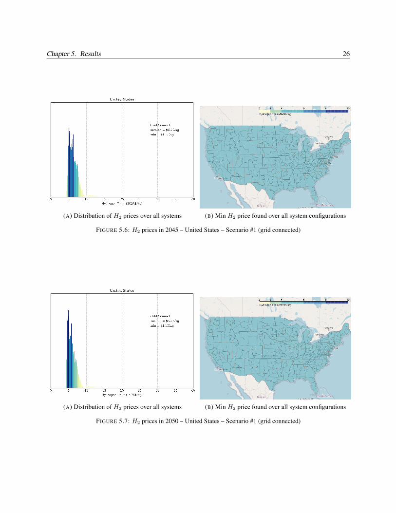
Chapter 5. Results 26
(A) Distribution of H2 prices over all systems (B) Min H2 price found over all system configurations
FIGURE 5.6: H2 prices in 2045 – United States – Scenario #1 (grid connected)
(A) Distribution of H2 prices over all systems (B) Min H2 price found over all system configurations
FIGURE 5.7: H2 prices in 2050 – United States – Scenario #1 (grid connected)

Chapter 5. Results 27
5.1.2 Europe - Hydrogen Prices
(A) Distribution of H2 prices over all systems (B) Min H2 price found over all system configurations
FIGURE 5.8: H2 prices in 2020 – Europe – Scenario #1 (grid connected)
(A) Distribution of H2 prices over all systems (B) Min H2 price found over all system configurations
FIGURE 5.9: H2 prices in 2025 – Europe – Scenario #1 (grid connected)

Chapter 5. Results 28
(A) Distribution of H2 prices over all systems (B) Min H2 price found over all system configurations
FIGURE 5.10: H2 prices in 2030 – Europe – Scenario #1 (grid connected)
(A) Distribution of H2 prices over all systems (B) Min H2 price found over all system configurations
FIGURE 5.11: H2 prices in 2035 – Europe – Scenario #1 (grid connected)

Chapter 5. Results 29
(A) Distribution of H2 prices over all systems (B) Min H2 price found over all system configurations
FIGURE 5.12: H2 prices in 2040 – Europe – Scenario #1 (grid connected)
(A) Distribution of H2 prices over all systems (B) Min H2 price found over all system configurations
FIGURE 5.13: H2 prices in 2045 – Europe – Scenario #1 (grid connected)

Chapter 5. Results 30
(A) Distribution of H2 prices over all systems (B) Min H2 price found over all system configurations
FIGURE 5.14: H2 prices in 2050 – Europe – Scenario #1 (grid connected)

Chapter 5. Results 31
5.2 Scenario #2: Results
Recall that Scenario #2 assumes that the power-to-gas plant is connected to the renewable electricity gener-ator and therefore will run at the capacity factor of the generator but does not pay electricity costs associatedwith transmission and distribution. The results can be summarized as:
• The median price of H2 in the US will decrease from $10.61/kg in 2020 to $5.97/kg in 2050; duringthat same timeframe the minimum price decreases from $4.56/kg to $2.44/kg.
• The median price of H2 in the EU will decrease from $19.23/kg in 2020 to $10.02/kg in 2050; duringthat same timeframe the minimum price decreases from $4.06/kg to $2.23/kg.
The following figures show theH2 price distribution and the geographical distribution of theseH2 prices(and follow the same analytical logic discussed in section 5.1).
Figures 5.15-5.21 summarize the results for the United States between 2020-2050. Figures 5.22-5.28summarize the results for the European Union between 2020-2050.
5.2.1 United States - Hydrogen Prices
(A) Distribution of H2 prices over all systems (B) Min H2 price found over all system configurations
FIGURE 5.15: H2 prices in 2020 – United States – Scenario #2 (direct connection)

Chapter 5. Results 32
(A) Distribution of H2 prices over all systems (B) Min H2 price found over all system configurations
FIGURE 5.16: H2 prices in 2025 – United States – Scenario #2 (direct connection)
(A) Distribution of H2 prices over all systems (B) Min H2 price found over all system configurations
FIGURE 5.17: H2 prices in 2030 – United States – Scenario #2 (direct connection)

Chapter 5. Results 33
(A) Distribution of H2 prices over all systems (B) Min H2 price found over all system configurations
FIGURE 5.18: H2 prices in 2035 – United States – Scenario #2 (direct connection)
(A) Distribution of H2 prices over all systems (B) Min H2 price found over all system configurations
FIGURE 5.19: H2 prices in 2040 – United States – Scenario #2 (direct connection)

Chapter 5. Results 34
(A) Distribution of H2 prices over all systems (B) Min H2 price found over all system configurations
FIGURE 5.20: H2 prices in 2045 – United States – Scenario #2 (direct connection)
(A) Distribution of H2 prices over all systems (B) Min H2 price found over all system configurations
FIGURE 5.21: H2 prices in 2050 – United States – Scenario #2 (direct connection)

Chapter 5. Results 35
5.2.2 Europe - Hydrogen Prices
(A) Distribution of H2 prices over all systems (B) Min H2 price found over all system configurations
FIGURE 5.22: H2 prices in 2020 – Europe – Scenario #2 (direct connection)
(A) Distribution of H2 prices over all systems (B) Min H2 price found over all system configurations
FIGURE 5.23: H2 prices in 2025 – Europe – Scenario #2 (direct connection)

Chapter 5. Results 36
(A) Distribution of H2 prices over all systems (B) Min H2 price found over all system configurations
FIGURE 5.24: H2 prices in 2030 – Europe – Scenario #2 (direct connection)
(A) Distribution of H2 prices over all systems (B) Min H2 price found over all system configurations
FIGURE 5.25: H2 prices in 2035 – Europe – Scenario #2 (direct connection)

Chapter 5. Results 37
(A) Distribution of H2 prices over all systems (B) Min H2 price found over all system configurations
FIGURE 5.26: H2 prices in 2040 – Europe – Scenario #2 (direct connection)
(A) Distribution of H2 prices over all systems (B) Min H2 price found over all system configurations
FIGURE 5.27: H2 prices in 2045 – Europe – Scenario #2 (direct connection)

Chapter 5. Results 38
(A) Distribution of H2 prices over all systems (B) Min H2 price found over all system configurations
FIGURE 5.28: H2 prices in 2050 – Europe – Scenario #2 (direct connection)

Chapter 5. Results 39
5.3 Scenario #3: Results
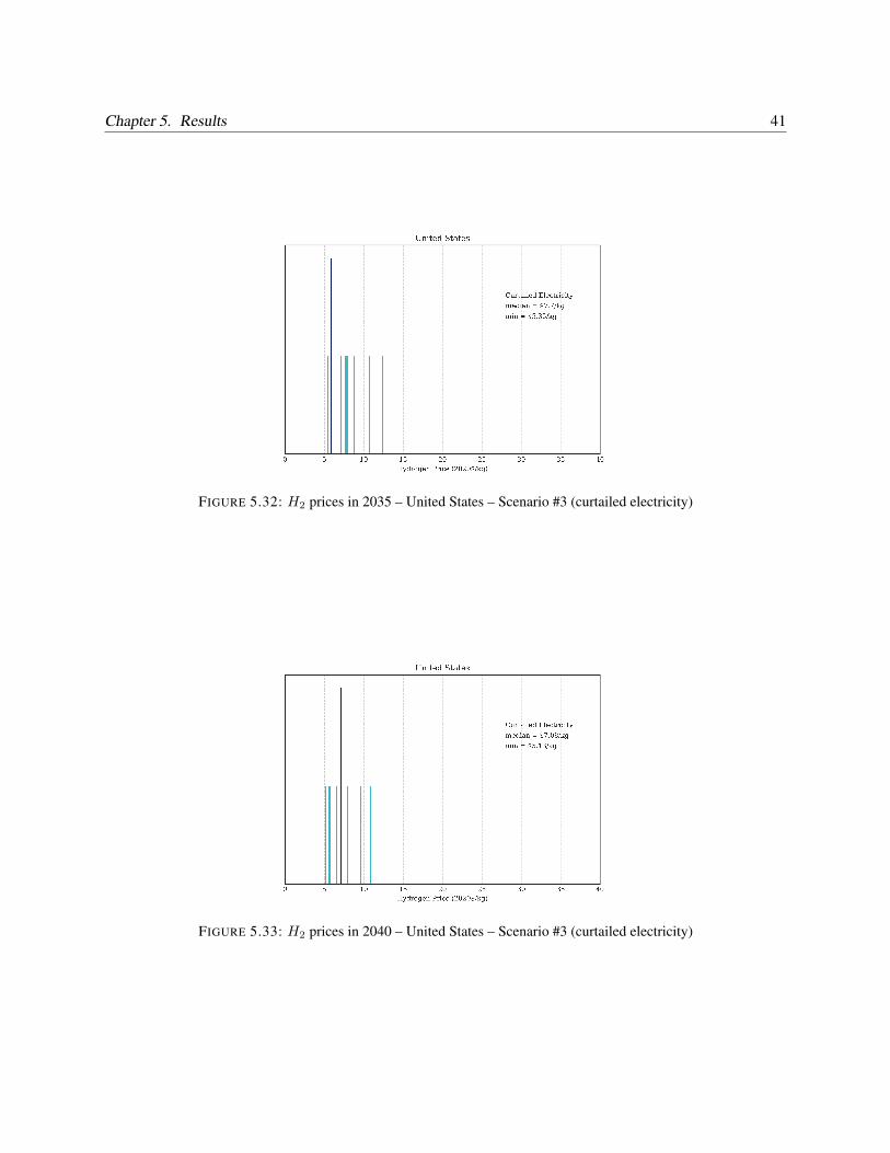
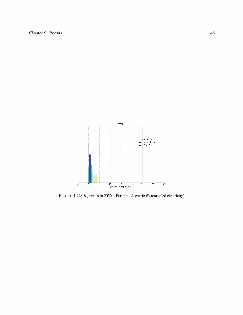
Recall that Scenario #3 assumes that the power-to-gas plant is connected to the transmission grid, but onlydraws energy when renewable energy must be curtailed (assumed to be 4 hours per day = 16% capacityfactor). The curtailed electricity is considered to be free ($0/kWh). The histograms do not show as widea distribution as a result of the capacity factor being equalized across all regions – variation is only due todifferences in technology configurations and tax rates. The results can be summarized as:
• The median price of H2 in the US will decrease from $11.02/kg in 2020 to $5.92/kg in 2050; duringthat same timeframe the minimum price decreases from $6.10/kg to $4.75/kg.
• The median price of H2 in the EU will decrease from $10.85/kg in 2020 to $6.08/kg in 2050; duringthat same timeframe the minimum price decreases from $5.97/kg to $4.67/kg.
5.3.1 United States - Hydrogen Prices
FIGURE 5.29: H2 prices in 2020 – United States – Scenario #3 (curtailed electricity)

Chapter 5. Results 40
FIGURE 5.30: H2 prices in 2025 – United States – Scenario #3 (curtailed electricity)
FIGURE 5.31: H2 prices in 2030 – United States – Scenario #3 (curtailed electricity)
Chapter 5. Results 41
FIGURE 5.32: H2 prices in 2035 – United States – Scenario #3 (curtailed electricity)
FIGURE 5.33: H2 prices in 2040 – United States – Scenario #3 (curtailed electricity)

Chapter 5. Results 42
FIGURE 5.34: H2 prices in 2045 – United States – Scenario #3 (curtailed electricity)
FIGURE 5.35: H2 prices in 2050 – United States – Scenario #3 (curtailed electricity)

Chapter 5. Results 43
5.3.2 Europe - Hydrogen Prices
FIGURE 5.36: H2 prices in 2020 – Europe – Scenario #3 (curtailed electricity)
FIGURE 5.37: H2 prices in 2025 – Europe – Scenario #3 (curtailed electricity)

Chapter 5. Results 44
FIGURE 5.38: H2 prices in 2030 – Europe – Scenario #3 (curtailed electricity)
FIGURE 5.39: H2 prices in 2035 – Europe – Scenario #3 (curtailed electricity)

Chapter 5. Results 45
FIGURE 5.40: H2 prices in 2040 – Europe – Scenario #3 (curtailed electricity)
FIGURE 5.41: H2 prices in 2045 – Europe – Scenario #3 (curtailed electricity)
Chapter 5. Results 46
FIGURE 5.42: H2 prices in 2050 – Europe – Scenario #3 (curtailed electricity)

47
Chapter 6
Study Comparison
There are a number of economic parameters that are needed in order to fully define the technical and eco-nomic performance of a power-to-gas system; these parameters are detailed in Chapter 5. Parameter valuedifferences will result in discrepancies when directly comparing studies, however, it is also important to doc-ument the underlying set of assumptions that each study uses in order to more fairly compare results. Thischapter is dedicated to documenting the set of assumptions used by three prominent studies by the Inter-national Energy Agency (IEA), Bloomberg New Energy Finance (BNEF), and the International RenewableEnergy Agency (IRENA) [5, 6, 7].
6.1 Summary of Results from IEA Report
The main results from the IEA that are of concern to this work are summarized in four Figures: 12, 13, 14,and 16. We will take each of these figures in turn and describe their results and compare them to assumptionsmade in this work.
In sum, the IEA report ignores important system costs that are associated with building out a fullyoperational H2 electrolysis plant, at the same time their electricity price projections are more optimisticthan even the most optimistic scenario produced by NREL in the Annual Technology Baseline.
6.1.1 IEA Future of Hydrogen – Figure 12

Chapter 6. Study Comparison 48
FIGURE 6.1: IEA – Figure 12, reproduced from [5]
Figure 12 is captioned “Future levelised cost of hydrogen (LCOH) production by operating hour fordifferent electrolyser investment costs (left) and electricity costs (right)” and shows theH2 ($/kg) sensitivityto different capacity factors (0.0-0.91), electrolyzer CAPEX costs ($250-650/kW), and electricity prices (0-100 MWh). These graphs were produced under an 8% hurdle rate assumption and an electrolyzer efficiencyof 69%. It is unclear what year these H2 production prices are supposed to represent. It is up to the readerto infer from the Assumption Annex and Table 3 (page 44-45) that the sensitivity values probably representa “Long Term” view of H2 production costs under an optimistic cost reduction scenario.
There is also no discussion of the assumed source of electricity that could provide the range of pricesthat IEA includes in this sensitivity test. In this work, we do project electricity prices to be as low as≈ $0.03/kWh from onshore wind generators, but the capacity factor would be limited to 0.69 (6044 hours)– this example correspondes to Swedish wind resources. Capacity factors shown in Figure 12 above thisrange would require grid connections and therefore would likely need to pay transmission and distributioncharges. These charges, without considering the cost of actually producing the renewable electricity, wouldbe enough to push the electricity price toward the maximum values that were considered by IEA.
There is little discussion of the methodologies used to project the CAPEX costs, although IEA doesstate that “Parameters for the cost and performance of technologies have been based on extensive literatureanalysis, conversations with experts and peer review.” The present study uses historical cost trend to projectCAPEX costs out to 2050 (with uncertainty). IEA uses CAPEX values for AE systems that range between500 $/kW (in 2020) to 200 $/kW in 2050; the present study builds scenarios that use CAPEX values between571-1268 $/kW in 2020 and 487-1090 $/kW in 2050. More details on other systems can be found in Table4.3.
While these graphs present the “production” costs, it is up to the reader to interpret exactly what ismeant by “production”. We were able to reproduce the IEA data shown in Figure 12 with our financialmodel framework and incorporating the IEA assumptions, but only if we neglected all system costs beyondthe electricity and electrolyzer CAPEX costs. This is in contrast to this work, which only presents H2

Chapter 6. Study Comparison 49
prices as produced, compressed (w/short-term on-site storage) and injected into a pipeline distribution sys-tem. Production of H2, as described in Chapter 4, includes costs from – electrolyzer CAPEX, electrolyzerreplacement (if necessary), electricity, water, piping, compressor CAPEX, storage, and other fixed OPEXcosts.
A casual reader or policy maker could easily overlook the missing costs, unclear timeframe, and opti-mistic electricity prices and draw some incomplete conclusions as to the economic viability of H2 produc-tion.
6.1.2 IEA Future of Hydrogen – Figure 13
FIGURE 6.2: IEA – Figure 13, reproduced from [5]
Figure 13 is captioned “Hydrogen costs from electrolysis using grid electricity” and shows the H2 pro-duction costs for an electrolyzer that was $800/kW and 64% efficient. Figure 13 does clarify that theelectricity is provided from the grid (electricity prices from Japan) and therefore the electricity prices arein a range that would be expected even in the US or Europe (as was the focus of this work). As such, thehydrogen production prices are much closer to those calculated in this work. Their hydrogen prices rangefrom a minimum of ≈ $8/kg to above $20/kg of H2. These values align with the values produced in thiswork, although it is unclear if their methodologies capture all the cost details that are presented here. Theprimary conclusion of this graph is that electricity use is the primary driver of H2 price, a conclusion thatthis work also agrees with.
6.1.3 IEA Future of Hydrogen – Figure 14

Chapter 6. Study Comparison 50
FIGURE 6.3: IEA – Figure 14, reproduced from [5]
Figure 14 is captioned “Hydrogen costs from hybrid solar PV and onshore wind systems in the longterm” and shows the geographical distribution of H2 prices from a simple power-to-gas system. IEA statesthat the model used to generate these prices assume the electrolyser CAPEX to be $450/kW (74% efficient,an optimistic assumption). Solar PV CAPEX and onshore wind CAPEX vary by region and range between$400–1000/kW and $900–2500/kW, respectively. The hurdle rate is assumed to be 8%.
While it is important to understand the geographical distribution of these resources, the description ofthe assumptions used to generate this figure are insufficient. Specifically, it is unclear what capacity factora “hybrid” system would be able to achieve. It is also unclear what, if any, other costs are included in thisanalysis and for what year this data is supposed to represent (other than “in the long term”). From the rangeof prices in the legend it is left to the reader to infer that, again, this is an optimistic scenario in terms of bothcapacity factor and electrolyzer CAPEX cost. As with Figure 12, a time-strapped analyst or policy makercould easily overlook the missing costs, unclear timeframe, and optimistic electricity prices and draw someincomplete conclusions as to the economic viability of H2 production.
6.1.4 IEA Future of Hydrogen – Figure 16

Chapter 6. Study Comparison 51
FIGURE 6.4: IEA – Figure 16, reproduced from [5]
Figure 16 is captioned “Hydrogen production costs for different technology options, 2030” and showsthe hydrogen price for several different pathways; we are interested in the “Electrolysis grid” and “Electrol-ysis renewable” scenarios. IEA states that this figure assumed an electricity price of $40/MWh and 4000 fullload hours (capacity factor = 0.45); uncertainty is assumed to be a fixed ±30%. While not explicitly stated,IEA does make reference to the Assumptions Annex for further information. When the reader arrives at theAnnex, it is still unclear what values are used to produce Figure 16. It is left to the reader to infer that thecapacity factor used for the “electrolysis grid” scenario is 0.57 (5000 hours) and 0.23/0.27 (2054 hours forthe EU and 2425 hours for the US) for the “electrolysis renewable” scenario. The prices for electricity rangefrom $100-114/MWh for grid based electricity and $31-47/MWh for renewable electricity generators. Wecalculate electricity prices that are within these ranges, however, they occur later than 2030 as assumed herein Figure 16. Only the most optimistic scenario from NREL’s ATB result in renewable electricity prices thatare par with those used in “electrolysis renewable” scenario (see Figure 3.6-3.11).
The electrolyzer CAPEX cost is similarly unclear, but the Assumption Annex make reference to a 2030CAPEX cost of $700/kW for a “water electrolysis” system; it is unclear what type of electrolyzer this priceis supposed to represent. In this work we generally assume a CAPEX range between $365-2175/kW acrossall electrolyzer types in 2030.
The IEA results for “electrolysis grid” show that the price of H2 to be between $3.50-6.75/kg; the“electrolysis renewable” scenario shows a price of $2.00-4.00/kg. This work shows median in 2030 thatare $7.37/kg ($4.95/kg minimum) for a grid connected system; our direct connected results (for 2030) showa median value of $8.27/kg and a minimum price of $3.22/kg. Our price premium is primarily due to theaddition of other system costs that we include (compressor CAPEX, piping, water, etc.).

Chapter 6. Study Comparison 52
6.2 Summary of Results from Bloomberg New Energy Finance Report
The main results from the BNEF state that “with a scale-up in production of electrolyzers and optimizedpower supply for large-scale production, we forecast that the cost of producing renewable hydrogen couldfall to $1.4- 2.9/kg by 2030 and just $0.8-1.0/kg by 2050”. These figures ignore important system costs thatare associated with building out a fully operational H2 electrolysis plant and only focus on the electrolyzerCAPEX costs and costs associated with the purchase of electricity and water. While electricity price projec-tions are in general agreement with this current work the CAPEX price projections used by BNEF deviatefrom this current study and are much more optimistic. Additionally, these prices might only be achieveablein areas with idealized resource conditions (which may or may not be achieveable), something that wouldhinder widespread adoption.
6.2.1 Capital Costs for Chinese Electrolyzers
The BNEF report makes many mentions to the price differences between electrolyzers that were manufac-tured in China vs. those made in wester countries. Chinese electrolyzers are approximately 50% the cost ofthose electrolyzers built in western countries. This huge difference is explained by BNEF as:
• “Cheaper raw materials and labor. Labor is particularly important, as electrolyzers are still largelyhandmade.”
• “Higher factory utilization rates: The electrolyzer manufacturing industry in China is highly concen-trated, and the top three suppliers together have a 90% share of the domestic market. Demand for theirproducts (in traditional industries that require small-scale on-site pure hydrogen generation) is stableas it is linked with general manufacturing industry growth, which is much stronger in China than indeveloped countries. Chinese electrolyzer companies also have secure and predictable sales volumesand have a strong understanding about demand. As a consequence, their manufacturing capacity iswell-matched with the demand, resulting in high utilization rates, particularly for lines producinglarge electrolyzers.”
It is difficult to verify these claims since many of BNEF sources are references to their own work. Theliterature on electrolyzer costs that was reviewed in Chapter 4 makes no mention of this huge discrepancy inwestern vs. Chinese prices. Prices for large western-made AE and PEM electrolyzers generally agree withthose used in this work.
6.2.2 Modeling Assumptions and Technical Parameters
The BNEF report contains a summary table of all the benchmark costs and technical parameters that wereused in describing MW-scale electrolyzer systems. Most of these values present in this table are in generalagreement with the values that were used in this work to calculate the price of H2. Of note is that there areno costs associated with compression, piping, water, etc., the BNEF price calculations only include thosecosts associated with the electrolyzer itself.
The metric that is used by BNEF to describe the electricity consumption (kWh/kg of H2) is related tothe electrolyzer efficiency parameter that is more commonly used in other reports. The conversion between

Chapter 6. Study Comparison 53
the two numbers can be calculated as Electricity Consumption (kWh/kg H2) = [η(ideal yield rate)]−1. Theideal yield rate is simply 0.03 kg of H2/kWh and is calculated by converting the energy density of H2
(120 MJ/kg) to units of kWh/kg and taking the reciprocal. The BNEF report assumes that the electricityconsumption rate is 53 kWh/kg of H2, which is equivalent to a 63% efficient electrolyzer. This conversionefficiency also agrees with values in this work.
Of note is the electrolyzer capacity factor (91%); this high number suggests that BNEF assumes thatthese systems will be grid connected, however BNEF does go on to produce other scenarios that are notnecessarily drawing electricity from the grid for 91% of the time. Care must be taken to inspect whendisucssing results so as to not to conflate two different subanalyses.
6.2.3 H2 Cost – Grid Connected/Continuous Operation
BNEF includes a subanalysis that aims to calculate the LCOH from grid-connected systems in continuousoperation in 2019. This subanalysis and details the price of H2 for different AE and PEM electrolyzersystems for 2019. BNEF calculates that the price of H2 should be in the range of $5.52-6.82 (2019$/kg)when electricity is priced at $0.10/kWh and the same 91% capacity factor (as mentioned previously) isassumed. We were able to reproduce these values with the set of BNEF assumptions.
While these prices are likely low because they omit other important costs, the price of electricity is areasonable value to assume given current grid prices and the potential for prices to be behave in the future.This subanalysis makes it clear that CAPEX costs are not the primary driver of H2 price, instead the cost ofelectricity accounts for more than 80% (or more) of the total cost of H2.
To provide further context, we specify a hypothetical system with $0 costs except for costs associatedwith the purchase of electricity. This system is illustrative in that we can get a sense of the lower bound ona kg of H2 based on only the price of electricity. If we generously assume that the conversion efficiencyis 80%, the system can achieve a 100% capacity factor, and electricity was $0.01/kWh the levelized costof hydrogen would be $0.83/kg. There are no scenarios in this work that would suggest that a price ofelectricity could ever (2020-2050) be purchased at $0.01/kWh for 100% of the time. Governments wouldneed to provide subsidies in order to ensure that power-to-gas plants could purchase electricity at rates thislow.
6.2.4 H2 Cost – Grid Connected/Off-Peak Electricity Prices
This subanalysis suggests that the LCOH operating with off-peak (grid-based) electricity would be between$2.75-5.02/kg. BNEF assumes that the power-to-gas plant uses electricity purchased during off-peak hours.This electricity is purchased at $0.045/kWh and comes with a capacity factor of 50%. We were able toverify the result presented here with our modeling framework.
6.2.5 H2 Cost – Grid Connected/Curtailed Electricity
This subanalysis looks at the LCOH as if it were produced from curtailed (zero-cost) electricity in 2019(similar to our Scenario #3). It is difficult to quantify the level of curtailed electricity, thus BNEF calculatesthe price of H2 for three different systems along a range of capacity factors (0-100%). We assume a 16%capacity factor for our curtailed electricity scenario. BNEF reported that the LCOH for a PEM (western

Chapter 6. Study Comparison 54
origin) would be $8.62, $5.46 for an AE system (western origin), and $1.13 for an AE system of Chineseorigin); these values were calculated using a 15% capacity factor assumption.
6.2.6 H2 Cost – Direct Connection to a Renewable Electricity Generator
This subanalysis looks at the levelized cost ofH2 as if it were directly connected to a wind generator (similarto our Scenarion #2). BNEF optimizes the geneator configuration in order to increase the effective capacityfactor. To achieve a higher utilization rate of the electrolyzer BNEF identifies three options:
• Oversize the renewable generator, which causes curtailment during times of max output, but resultsin more energy delivery in periods below max output, increasing the overall utilization.
• Couple wind and PV generators to take advantage of the typical negative correlation between PV andwind generation profiles (the wind often blows when the sun does not shine).
• Add batteries to enable supply at times when generators are not producing. This action can only boostthe electrolyzer’s utilization rate when power generators are oversized.
BNEF concludes that the most cost-effective approach is to couple wind and PV generation, but theygo on to recognize that this may not be an option in all locations. For this subanalysis it is unclear exactlywhich system configuration is used to achieve the capacity factors and electricity prices that are summarizedin Table 6.1. BNEF does mention that “The LCOH values shown in [Figure 21 in the BNEF report] arebased on separate system optimizations for the three equipment options, which result in different wind farmcapacities (assuming the same capacity for the three electrolyzers) and therefore different power pricesand utilization rates for the electrolyzers. Oversizing the wind farm leads to curtailment and a higherLCOE; meanwhile, the electrolyzer can operate with a higher utilization rate and achieve a lower levelizedcost of equipment per unit of hydrogen produced. The system is optimized between electricity cost andequipment cost, which depends on electrolyzer capex, fixed opex, the levelized cost of the wind plant withoutcurtailment, and the output profile of the wind farm. For the example analysis here, we assumed a $40/MWhLCOE (no curtailment) from a wind farm in California, with an annual capacity factor of 38% (hourlygeneration profile extracted from California Independent System Operator’s 2018 wind output). A highutilization rate is more valuable (or economically worthy) in an expensive system, despite a high coupledLCOE. In this example, the optimal utilization rate for the Western-made PEM system is 62%, while that forthe Chinese-made alkaline is 51%.” [6].

Chapter 6. Study Comparison 55
TABLE 6.1: LCOH Summary from the BNEF Report
Scenario Electrolyzer CF Electricity ($/kWh) LCOH ($/kg)
Grid Connected AE (Chinese) 91% $0.10/kWh $5.52/kgGrid Connected AE (Western) 91% $0.10/kWh $6.20/kgGrid Connected PEM (Western) 91% $0.10/kWh $6.82/kg
Grid Connected/Off-Peak AE (Chinese) 50% $0.045/kWh $2.75/kgGrid Connected/Off-Peak AE (Western) 50% $0.045/kWh $4.03/kgGrid Connected/Off-Peak PEM (Western) 50% $0.045/kWh $5.02/kg
Curtailed Electricity AE (Chinese) 15% $0.00/kWh $1.13/kgCurtailed Electricity AE (Western) 15% $0.00/kWh $5.46/kgCurtailed Electricity PEM (Western) 15% $0.00/kWh $8.62/kg
Direct Connection AE (Chinese) 51% $0.0409/kWh $2.53/kgDirect Connection AE (Western) 58% $0.0437/kWh $3.72/kgDirect Connection PEM (Western) 62% $0.0459/kWh $4.57/kg
6.2.7 Electricity Price Projections
BNEF states “we project that PV and/or wind could provide electricity to a large-scale electrolyzer forjust $24-28/MWh [$0.024-0.028/kWh] by 2030 and $15-17/MWh [$0.015-0.017/kWh] by 2050.” Basedon price paths shown in the report, it appears that the first price range of $24-28/MWh is based on solargenerators in India, while the $15-17/MWh price range appears to be based on onshore wind in India.
The electricity price paths (2019-2050) do detail other country-specific electricity price paths, but exactnumerical comparisons are difficult due to the resolution of the graphs. The present study calculates that thelowest solar PV electricity price would be $34/MWh (US) and $42/MWh (EU) in 2030 and $22/MWh (US)and $27/MWh (EU) in 2050. The present study also calculates that the lowest onshore wind electricity pricewould be $27/MWh (US) and $23/MWh (EU) in 2030 and $19/MWh (US) and $16/MWh (EU) in 2050.
Caution should be taken when referencing these prices because they are the minimum prices calculatedfor a region, the median price of electricity could be much higher. These price paths are also not directlyused in the creation of the LCOH in any of the subanalyses introduced in Sections 6.2.3, 6.2.4, 6.2.5, 6.2.6.
6.2.8 CAPEX Forecasting
BNEF, like others, including our work, attempt to forecast the system CAPEX for large-scale electrolysisprojects. There are several sections of this report that are dedicated to this single economic parameter.While there are main details that could be covered, we state here that the CAPEX reduction pathways from2019-2050 and again highlight the fact that BNEF assumes that Chinese electrolyzers are dramatically lessexpensive than other western-made systems. Some of the CAPEX price points that were detailed by BNEFare included in Table 4.3 alongside the values used in this current work. Of note is that BNEF assumesthat there will be a cost convergence between the western and Chinese systems in 2030, where their priceswill equalize out at the lower Chinese price. There is no justification provided for this assumption. These

Chapter 6. Study Comparison 56
trajectories also are much more aggressive than historical cost reduction patterns examined by Glenk et al[12]; this work relies on CAPEX projections that mimic historical behavior
6.3 Summary of Results from IRENA Report
The main results from the IRENA report that are of concern to this work are summarized in four figures (9,10, 11, 14). As we did with the other report summaries, we will take each of these references in turn anddescribe their results and compare them to assumptions made in this work.
In sum, the IRENA report ignores important system costs that are associated with building out a fullyoperational H2 electrolysis plant, at the same time their electricity price projections are more optimisticthan even the most optimistic scenario produced by NREL in the Annual Technology Baseline. Many oftheir price scenarios and capacity factors represent a “global best”, which highlights the importance of beingexplicit about the geographic extent of the analysis.
6.3.1 IRENA – Figure 9
FIGURE 6.5: IRENA – Figure 9, reproduced from [7]
Figure 9 is captioned “Hydrogen costs at different electricity prices and electrolyser Capex” and shows,at a high level, what the H2 price would be under different electrolyzer costs and electricity prices. Forthese calculations they assume a capacity factor of 40%. IRENA uses different combinations of elec-trolyzer/electricity prices to forecast H2 prices out to 2050. They assume an electrolyzer price of $840/kWand electricity costs at $0.04/kWh for current day calculations. These prices are scaled down to $200/kWand electricity costs at $0.20/kWh for 2050 projections.
The electricity prices used in this graph are overly optimistic in that they follow a path below the mostoptimistic price projection pathway from NREL’s ATB dataset. The capacity factor that is used for thesesimulations also reflects a “best case” scenario for the renewable electricity generator (while not explicitly

Chapter 6. Study Comparison 57
stated in this figure, it is likely that they assume electricity is delivered through a direct connection to a windgenerator). It should not be assumed that this capacity factor is available at all geographical locations.
We have verified that the values reported here are correctly calculated, but like other reports, the lowprice of H2 could be considered misleading through the combination of overly optimistic electricity pricesand ignoring other system costs; the IRENA report only assumes costs associated with the actual electrolyzerand the purchase of electricity.
6.3.2 IRENA – Figure 10
FIGURE 6.6: IRENA – Figure 10, reproduced from [7]
Figure 10 is captioned “Costs of producing hydrogen from renewables and fossil fuels today” and com-pares the costs associated with many different types of H2 pathways. We are primarily interested in theirestimates of H2 prices from their “Average” and “Low Cost” scenarios for wind and solar generators. Forthis figure IRENA assumes an electrolyzer price of $840/kW (65% efficient) and electricity costs range be-tween $0.0175-0.085/kWh. Wind generation is assumed to have a 48% capacity factor and solar is assumedto have a 26% capacity factor.
Again, IRENA assumes a combination of capacity factors for both wind and solar that should be consid-ered a global “best case” scenario. We agree with the electricity prices used for both of IRENA’s “Average”

Chapter 6. Study Comparison 58
scenarios, but again, these prices are more closely aligned with a “best case” US/EU scenario not an “aver-age”. The “low cost” scenarios produced by IRENA incorporate prices that are ≈ 1/4 of the most optimisticproduced by NREL for the US. They do recognize that “low-cost renewable power of USD 23/MWh is seentoday in wind projects in countries such as Brazil and Saudi Arabia”.
6.3.3 IRENA – Figure 11
FIGURE 6.7: IRENA – Figure 11, reproduced from [7]
Figure 11 is captioned “Cost of producing hydrogen from renewables and fossil fuels, 2018 and 2050”and shows the H2 price falling so that it is competitive with H2 production from fossil fuels. IRENA alsoassumes that there will be a price to pay for any emitted carbon ($50/ton and $200/ton) when producing H2,these added prices make H2 production from renewable electricity generators more economically viable.
There are a lot of assumptions detailed in this graph they are detailed in Table 6.2. Note that it is unclearwhy Figure 11 presents 2018 values, but the notes in the caption list 2030 data, we make no assumptionsas to the true meaning of the data and only reproduce IRENA’s table for comparison at face value. Whilethere is agreement between this work and IRENA’s “average” assumptions (Table 6.2) we still believe thatthe costs of H2 production are being under estimated as other systems costs have been ignored.

Chapter 6. Study Comparison 59
TABLE 6.2: Comparison of assumptions used in IRENA Figure 11.
Year Scenario Capacity Factor Electricity Price ($/kWh) Comparison to this work
2030 Wind (best) 47% 0.023 more optimistic2030 Wind (average) 34% 0.055 agreement2030 PV (best) 27% 0.018 much more optimistic2030 PV (average) 18% 0.085 agreement2050 Wind (best) 63% 0.011 more optimistic2050 Wind (average) 45% 0.023 more optimistic2050 PV (best) 27% 0.0045 much more optimistic2050 PV (average) 18% 0.022 agreement
6.3.4 IRENA – Figure 14
FIGURE 6.8: IRENA – Figure 14, reproduced from [7]
Figure 14 is captioned “Hydrogen production costs from solar and wind vs. fossil fuels” and shows theprice trajectories for various H2 production pathways from now until 2050. This graph explicitly states that“Low-cost solar and wind resources start to achieve fossil fuel parity within the next five years”. This boldclaim relies on assumptions that there are zero other system costs. It appears that this data was also calculatedusing the assumptions in Table 6.2, which have already been documented as being overly optimistic when

Chapter 6. Study Comparison 60
compared to the US and EU cases – IRENA considers the “best case” scenario to truly be the “globalbest”. This graph also assumes that carbon prices will impact the price of traditional H2 production fromfossil fuels; IRENA assumes carbon prices of $50/ton (2030), $100/ton (2040), and $200/ton (2050). Thesecarbon prices increase the cost of traditional H2 production and help make H2 production from renewableelectricity generators more economically viable.

61
Bibliography
[1] National Renewable Energy Laboratory. Annual Technology Baseline Dataset. URL: https://atb.nrel.gov/electricity/data.html.
[2] National Renewable Energy Laboratory. Renewable Energy Deployment System Model (ReEDS).URL: https://www.nrel.gov/analysis/reeds/.
[3] Iratxe Gonzalez Aparicio et al. “EMHIRES dataset Part II: Solar power generation”. In: EuropeanMeteorological derived High resolution RES generation time series for present and future scenarios.Part II: PV generation using the PVGIS model. EUR 28629 (2017).
[4] Iratxe Gonzalez Aparicio et al. EMHIRES dataset Part I: Wind power generation. Tech. rep. EuropeanCommission, 2016.
[5] IEA. The Future of Hydrogen. Tech. rep. Paris, 2019. URL: https://www.iea.org/reports/the-future-of-hydrogen.
[6] Bloomberg New Energy Finance. Hydrogen: The Economics of Production From Renewables. Tech.rep. 2019.
[7] IRENA. Hydrogen: A renewable energy perspective. Tech. rep. Paris, Sept. 2019. URL: https://www.irena.org/publications/2019/Sep/Hydrogen-A-renewable-energy-perspective.
[8] Vi Duong Dang and Meyer Steinberg. “Production of synthetic methanol from air and water usingcontrolled thermonuclear reactor power—II. Capital investment and production costs”. In: EnergyConversion 17.4 (1977), pp. 133–140.
[9] Meyer Steinberg. “Synthetic carbonaceous fuels and feedstocks from oxides of carbon and nuclearpower”. In: Fuel 57.8 (1978), pp. 460–468.
[10] Meyer Steinberg and Vi-Duong Dang. “Production of synthetic methanol from air and water usingcontrolled thermonuclear reactor power—I. Technology and energy requirement”. In: Energy Con-version 17.2-3 (1977), pp. 97–112.
[11] Selma Brynolf et al. “Electrofuels for the transport sector: a review of production costs”. In: Renew-able and Sustainable Energy Reviews (2017).
[12] Gunther Glenk and Stefan Reichelstein. “Economics of converting renewable power to hydrogen”.In: Nature Energy 4.3 (2019), pp. 216–222.
[13] N Lymberopoulos. “Hydrogen production from renewables”. In: Center for Renewable Energy Sources(CRES), Pikermi Attiki, Project Technical Assistant Framework Contract EESD Contract No: NNE5-PTA-2002-003/1 (2005).
[14] J I Levene. “Economic Analysis of Hydrogen Production from Wind: Preprint”. en. In: (), p. 20.

Bibliography 62
[15] C Brunetto and G Tina. “Optimal hydrogen storage sizing for wind power plants in day ahead elec-tricity market”. In: IET Renewable Power Generation 1.4 (2007). Publisher: IET, pp. 220–226.
[16] Christopher J Greiner, Magnus KorpÅs, and Arne T Holen. “A Norwegian case study on the produc-tion of hydrogen from wind power”. In: International Journal of Hydrogen Energy 32.10-11 (2007).Publisher: Elsevier, pp. 1500–1507.
[17] J Linnemann and R Steinberger-Wilckens. “Realistic costs of wind-hydrogen vehicle fuel produc-tion”. In: International Journal of Hydrogen Energy 32.10-11 (2007). Publisher: Elsevier, pp. 1492–1499.
[18] F Mueller-Langer et al. “Techno-economic assessment of hydrogen production processes for the hy-drogen economy for the short and medium term”. In: International Journal of Hydrogen Energy 32.16(2007). Publisher: Elsevier, pp. 3797–3810.
[19] Michael Wenske. “Wasserstoff–Herstellung per Elektrolyse”. In: 17th energie symposium. Citeseer,2008.
[20] Michael Sterner. Bioenergy and renewable power methane in integrated 100% renewable energysystems: Limiting global warming by transforming energy systems. Vol. 14. kassel university pressGmbH, 2009.
[21] Tom Smolinka, Martin Günther, and Jürgen Garche. Stand und Entwicklungspotenzial der Wasserelek-trolyse zur Herstellung von Wasserstoff aus regenerativen Energien: NOW-Studie: Kurzfassung desAbschlussberichts. Fraunhofer ISE, 2011.
[22] C Mansilla et al. “Reducing the hydrogen production cost by operating alkaline electrolysis as adiscontinuous process in the French market context”. In: International journal of hydrogen energy36.11 (2011). Publisher: Elsevier, pp. 6407–6413.
[23] Uwe Albrecht et al. “Analyse der Kosten Erneuerbarer Gase”. In: Eine Studie der Ludwig-Bölkow-Systemtechnik GmbH. Im Auftrag des Bundesverbandes Erneuerbare Energie eV (2013).
[24] F Graf et al. “Technoökonomische Studie von Power-to-Gas-Konzepten”. In: Deutschen Vereins desGas-und Wasserfaches (DVGW), Tech. Rep. (2014).
[25] C. Mansilla et al. “Economic competitiveness of off-peak hydrogen production today – A Europeancomparison”. en. In: Energy 55 (June 2013), pp. 996–1001. ISSN: 03605442. DOI: 10.1016/j.energy.2013.03.022. URL: https://linkinghub.elsevier.com/retrieve/pii/S0360544213002107 (visited on 04/16/2020).
[26] Gert Müller-Syring et al. “Entwicklung von modularen Konzepten zur Erzeugung, Speicherung undEinspeisung von Wasserstoff und Methan ins Erdgasnetz”. de. In: (), p. 350.
[27] Luca Bertuccioli et al. “Study on development of water electrolysis in the EU”. In: Fuel cells andhydrogen joint undertaking (2014).
[28] Mareike Jentsch, Tobias Trost, and Michael Sterner. “Optimal use of power-to-gas energy storagesystems in an 85% renewable energy scenario”. In: Energy Procedia 46.0 (2014). Publisher: Elsevier,pp. 254–261.
[29] Markus Lehner et al. Power-to-gas: technology and business models. Springer, 2014.

Bibliography 63
[30] H Steinmüller et al. “Power-to-Gas–eine Systemanalyse”. In: Markt-und Technologiescouting und–analyse.Energieinstitut an der Johannes Kepler Universität Linz, TU Wien, MU Leoben, JKU Linz (2014).
[31] Michael Sterner and Ingo Stadler. Energiespeicher-Bedarf, Technologien, Integration. Springer-Verlag,2014.
[32] Raphael Winkler-Goldstein and Aline Rastetter. “Power to gas: the final breakthrough for the hydro-gen economy?” In: Green 3.1 (2013). Publisher: De Gruyter, pp. 69–78.
[33] Behnam Zakeri and Sanna Syri. “Electrical energy storage systems: A comparative life cycle costanalysis”. In: Renewable and sustainable energy reviews 42 (2015). Publisher: Elsevier, pp. 569–596.
[34] Jecques De Bucy, O Lacroix, and L Jammes. “The potential of Power-to-Gas”. In: ENEA Consulting,Paris, France (2016).
[35] Manuel Götz et al. “Renewable Power-to-Gas: A technological and economic review”. In: Renewableenergy 85 (2016). Publisher: Elsevier, pp. 1371–1390.
[36] Wouter Vanhoudt et al. “Power-to-gas. Short term and long term opportunities to leverage synergiesbetween the electricity and transport sectors through power-to-hydrogen”. In: Hinicio SA and LBST-Ludwig-Bölkow-Systemtechnik GmbH (2016).
[37] Sean B Walker et al. “Benchmarking and selection of Power-to-Gas utilizing electrolytic hydrogen asan energy storage alternative”. In: International Journal of Hydrogen Energy 41.19 (2016). Publisher:Elsevier, pp. 7717–7731.
[38] Guido Pleßmann et al. “Global energy storage demand for a 100% renewable electricity supply”. In:Energy Procedia 46.0 (2014). Publisher: Elsevier, pp. 22–31.
[39] Mareike Jentsch. “Potenziale von Power-to-Gas Energiespeichern”. In: Fraunhofer-Institut für Winden-ergie und Energiesystemtechnik IWES, Stuttgart (2015).
[40] Verena Jülch. “Comparison of electricity storage options using levelized cost of storage (LCOS)method”. en. In: Applied Energy 183 (Dec. 2016), pp. 1594–1606. ISSN: 03062619. DOI: 10 .1016/j.apenergy.2016.08.165. URL: https://linkinghub.elsevier.com/retrieve/pii/S0306261916312740 (visited on 04/16/2020).
[41] D Steward et al. Lifecycle cost analysis of hydrogen versus other technologies for electrical energystorage. Tech. rep. National Renewable Energy Lab.(NREL), Golden, CO (United States), 2009.
[42] Stanko Hocevar and William Summers. “Hydrogen production”. In: Hydrogen technology. Springer,2008, pp. 15–79.
[43] Philippe Menanteau et al. “Une analyse économique de la production d’hydrogène à partir d’électricitééolienne pour des usages transport”. In: (2010).
[44] Chris Ainscough, David Peterson, and Eric Miller. “Hydrogen production cost from PEM electrol-ysis”. In: DOE Hydrogen and Fuel Cells Program Record, United States Department of Energy,Washington, DC (2014).
[45] Timothy E Lipman, Jennifer L Edwards, and Daniel M Kammen. “Fuel cell system economics: com-paring the costs of generating power with stationary and motor vehicle PEM fuel cell systems”. In:Energy Policy 32.1 (2004). Publisher: Elsevier, pp. 101–125.

Bibliography 64
[46] Alberto Varone and Michele Ferrari. “Power to liquid and power to gas: An option for the German En-ergiewende”. In: Renewable and Sustainable Energy Reviews 45 (2015). Publisher: Elsevier, pp. 207–218.
[47] Benjamin Guinot et al. “Profitability of an electrolysis based hydrogen production plant providinggrid balancing services”. In: International Journal of Hydrogen Energy 40.29 (2015). Publisher: El-sevier, pp. 8778–8787.
[48] Max Wei et al. A total cost of ownership model for low temperature PEM fuel cells in combined heatand power and backup power applications. Tech. rep. Lawrence Berkeley National Lab.(LBNL),Berkeley, CA (United States), 2014.
[49] Bent Sørensen et al. “Hydrogen as an energy carrier: scenarios for future use of hydrogen in the Dan-ish energy system”. In: International Journal of Hydrogen Energy 29.1 (2004). Publisher: Elsevier,pp. 23–32.
[50] Annabelle Brisse and Josef Schefold. “High temperature electrolysis at EIFER, main achievementsat cell and stack level”. In: Energy Procedia 29 (2012). Publisher: Elsevier, pp. 53–63.
[51] Brian vad Mathiesen et al. “Technology data for high temperature solid oxide electrolyser cells, alkaliand PEM electrolysers”. In: (2013). Publisher: Department of development and planning, AalborgUniversity.
[52] Michael Penev, Jarett Zuboy, and Chad Hunter. “Economic analysis of a high-pressure urban pipelineconcept (HyLine) for delivering hydrogen to retail fueling stations”. In: Transportation Research PartD: Transport and Environment 77 (2019). Publisher: Elsevier, pp. 92–105.
[53] Inc Nexant. “H2A Hydrogen Delivery Infrastructure Analysis Models and Conventional PathwayOptions Analysis Results”. In: (2008). Publisher: US Department of Energy Washington DC.
[54] Jean André et al. “Time development of new hydrogen transmission pipeline networks for France”.In: International journal of hydrogen energy 39.20 (2014). Publisher: Elsevier, pp. 10323–10337.
[55] Wade A Amos. Costs of storing and transporting hydrogen. Tech. rep. National Renewable EnergyLab., Golden, CO (US), 1999.
[56] Energy Information Administration. Assumptions to the Annual Energy Outlook: 2017. Tech. rep.2017. URL: https://www.eia.gov/outlooks/aeo/assumptions/pdf/0554(2017).pdf.