Different splitting techniques with application to air pollution models
Upload
khangminh22Category
view
2download
0
Assessment of different optimization techniques for the structural
components of a mining truck
Master en Ingeniería Mecánica Aplicada y Computacional
Universidad Pública de Navarra
Junio de 2015
Autora: Paula Aranzadi de Miguel
Director: Francisco Javier García Zabalegui

Master Universitario en Ingeniería Mecánica Aplicada y Computacional
Junio de 2015
2 |
1 INDEX
1.1 INDEX OF CONTENTS
1 Index ............................................................................................................................. 2
1.1 Index of contents................................................................................................... 2
1.2 Index of figures ...................................................................................................... 4
1.3 Index of tables ....................................................................................................... 7
1.4 Index of equations ................................................................................................. 7
2 Aim and scope .............................................................................................................. 9
3 Introduction ................................................................................................................ 10
3.1 Mining truck description ..................................................................................... 10
3.1.1 Load calculation ............................................................................................. 11
3.2 Optimization ........................................................................................................ 14
3.2.1 Topology optimization ................................................................................... 14
3.2.2 Shape optimization ........................................................................................ 16
3.2.3 Engine of the optimization analysis .............................................................. 16
3.3 Altair .................................................................................................................... 20
3.3.1 Inspire – Simplified topology optimization ................................................... 20
3.3.2 OptiStruct – Topology, topography, shape and size optimization ................ 20
3.3.3 HyperStudy – Multi-disciplinary deign exploration tool ............................... 21
4 Optimization in different parts of mining trucks ........................................................ 22
4.1 Topology optimization – Control arm– Inspire ................................................... 22
4.1.1 Definition of the model ................................................................................. 22
4.1.2 Design concept – Results interpretation ....................................................... 34

Assessment of different optimization techniques for the structural components of a mining truck
Paula Aranzadi de Miguel
| 3
4.1.3 Translation into real CAD geometry .............................................................. 41
4.1.4 Analysis in Pro/MECHANICA .......................................................................... 42
4.1.5 Comparison to former design – Evaluation of the design quality................. 51
4.1.6 Best practices, conclusions and future steps ................................................ 54
4.1.7 Discussion about how to include fatigue calculation .................................... 55
4.2 Parametric optimization – Frame – HyperStudy / ANSYS Workbench ............... 62
4.2.1 Discrete variables – Shell thicknesses parameterization .............................. 66
4.2.2 Optimization algorithm ................................................................................. 68
4.2.3 Discussion: how to optimize based on durability analysis with Virtual Lab Durability 69
4.3 Advanced topology and fine-tuning optimization - OptiStruct .......................... 71
4.3.1 Topology in OptiStruct .................................................................................. 71
4.3.2 Topography optimization .............................................................................. 72
4.3.3 Shape optimization ........................................................................................ 73
4.3.4 Size optimization ........................................................................................... 74
4.3.5 Free-sizing ...................................................................................................... 75
4.3.6 Free-shape ..................................................................................................... 75
4.3.7 ANSYS frame model ....................................................................................... 75
5 Conclusions ................................................................................................................. 77
5.1 Conclusions about the different optimization techniques based on FEA ........... 77
5.2 Conclusion about Altair software for optimization............................................. 78
6 Bibliographic references ............................................................................................. 79

Master Universitario en Ingeniería Mecánica Aplicada y Computacional
Junio de 2015
4 |
1.2 INDEX OF FIGURES
FIGURE 1.- Truck overall dimensions ...................................................................... 10
FIGURE 2.- Truck overview ............................................................................................. 10
FIGURE 3.- Gradient based methods .............................................................................. 16
FIGURE 4.- Difficulty of gradient based methods in searching the global optima ......... 17
FIGURE 5.- Original Control Arm FE model .................................................................... 22
FIGURE 6.- Design Space definition ................................................................................ 23
FIGURE 7.- Non-design space definition ........................................................................ 24
FIGURE 8.- Shape controls – manufacturing process constraint ................................... 24
FIGURE 9.- Control arm main load – bending moment ................................................. 26
FIGURE 10.- Kingpin housing (or Spindle) vertical displacement constraint ................. 27
FIGURE 11.- Kingpin housing (or Spindle) load, weighted link ....................................... 27
FIGURE 12.- Suspension strut load, weighted link ......................................................... 28
FIGURE 13.- Frame pin bearings displacement constraints ........................................... 29
FIGURE 14.- Bearings modelization trick for allowing rotation ..................................... 29
FIGURE 15.- Stress distribution comparison between former contact analysis in Pro/MECHANICA (left) and new linear boundary conditions in Inspire (right) – Same legend scale used 30
FIGURE 16.- Displacement contour plot comparison between former contact analysis in Pro/MECHANICA (left) and new linear boundary conditions in Inspire (right) ............................ 31
FIGURE 17.- Model and load cases to be used for the optimization analysis ................ 32
FIGURE 18.- Optimization analysis setup ....................................................................... 32
FIGURE 19.- Objective function: minimize mass ............................................................ 33
FIGURE 20.- Material definition in Inspire ..................................................................... 34
FIGURE 21.- Stress constraint: minimum safety factor (σy /σ) ....................................... 34

Assessment of different optimization techniques for the structural components of a mining truck
Paula Aranzadi de Miguel
| 5
FIGURE 22.- Thickness constraint: minimum thickness ................................................. 34
FIGURE 23.- Topology concept design of the control arm (Inspire) .............................. 35
FIGURE 24.- Terminology given to the concept design of the control arm ................... 36
FIGURE 25.- Safety factor contour plot for the design concept of the control arm under LC01 (Inspire) 37
FIGURE 26.- Safety factor contour plot for the design concept of the control arm under LC01 frame pin constraints reversed (Inspire).............................................................................. 38
FIGURE 27.- Safety factor contour plot for the design concept of the control arm under LC13 (Inspire) 39
FIGURE 28.- Safety factor contour plot for the design concept of the control arm under LC03 (Inspire) 40
FIGURE 29.- Safety factor contour plot for the design concept of the control arm under LC04 (Inspire) 41
FIGURE 30.- Comparison between concept design given by Inspire (left) and CAD geometry created in Pro/ENGINEER based on the concept design (right) .................................. 42
FIGURE 31.- Comparison between former design of the control arm and CAD geometry of the concept design in Pro/ENGINEER ....................................................................................... 42
FIGURE 32.- Mesh of the model ..................................................................................... 43
FIGURE 33.- P-Level results for all the edges in the model ............................................ 44
FIGURE 34.- Von Mises stress contour plot of the optimized control arm under LC01, linear static analysis in Pro/MECHANICA ...................................................................................... 45
FIGURE 35.- Von Mises stress contour plot of the optimized control arm under LC01, linear static analysis in Pro/MECHANICA ...................................................................................... 46
FIGURE 36.- Von Mises stress contour plot of the optimized control arm under LC03, linear static analysis in Pro/MECHANICA ...................................................................................... 47
FIGURE 37.- Von Mises stress contour plot of the optimized control arm under LC03, non-linear static contact analysis in Pro/MECHANICA ................................................................. 48
FIGURE 38.- Von Mises stress contour plot of the optimized control arm under LC03, non-linear static contact analysis in Pro/MECHANICA ................................................................. 49

Master Universitario en Ingeniería Mecánica Aplicada y Computacional
Junio de 2015
6 |
FIGURE 39.- Further work on the CAD geometry of the optimized control arm compared to first Pro/ENGINEER geometry .................................................................................................. 49
FIGURE 40.- Further work on the CAD geometry of the optimized control arm compared to Inspire design concept .............................................................................................................. 50
FIGURE 41.- Stress contour plot under LC01 for the second attempt of CAD geometry 50
FIGURE 42.- Comparison of former control arm (left) and optimized control arm (right) under load case LC01. Von Mises stress contour plot, non-linear contact analysis .................... 52
FIGURE 43.- Comparison of former control arm (left) and optimized control arm (right) under load case LC03. Von Mises stress contour plot, non-linear contact analysis .................... 52
FIGURE 44.- Comparison of former control arm (left) and optimized control arm (right) under load case LC13. Von Mises stress contour plot, non-linear contact analysis .................... 53
FIGURE 45.- Summary workflow for including optimization during design process ..... 54
FIGURE 46.- Maximum allowable stress amplitude S for a particular number of occurrences N 56
FIGURE 47.- Time series or load history of varying amplitude ...................................... 58
FIGURE 48.- Time series or load history of constant amplitude .................................... 59
FIGURE 49.- Pseudo - SN curve representing combinations of load range and number of occurrences with same level of damage ...................................................................................... 59
FIGURE 50.- Maximum allowable stress for N occurrences based on SN curve ............ 60
FIGURE 51.- Frame parts description and terminology ................................................. 63
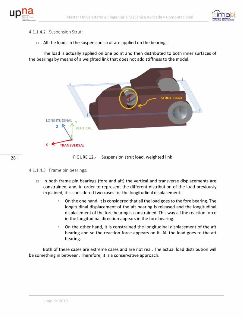
FIGURE 52.- Optimization of plate thicknesses .............................................................. 64
FIGURE 53.- Steel sheets distribution in order to minimize the sheet waste ................ 64
FIGURE 54.- Optimization of the shape of the steel sheets ........................................... 65
FIGURE 55.- Definition of parameters in ANSYS Workbench ......................................... 66
FIGURE 56.- Parametrization in ANSYS Workbench of the model Mass (objective function) 67
FIGURE 57.- Parameterization in ANSYS Workbench of the equivalent stress (response monitored for the optimization constraints) ................................................................................ 67

Assessment of different optimization techniques for the structural components of a mining truck
Paula Aranzadi de Miguel
| 7
FIGURE 58.- Definition of shell thickness as parameters (design variables) .................. 68
FIGURE 59.- Example of topography optimization on a container ................................ 73
FIGURE 60.- Example of shape optimization that helps to relieve stress concentrations around holes 73
FIGURE 61.- Optimization of frame walls internal reinforcement position ................... 74
1.3 INDEX OF TABLES
TABLE 1.- Durability schedule ......................................................................................... 12
TABLE 2.- Quasi-static load cases (LC) ............................................................................ 13
TABLE 3.- Example of quasi-static contemporaneous load table .................................. 13
TABLE 4.- Ultimate extreme load envelope ................................................................... 25
1.4 INDEX OF EQUATIONS
[1] ...................................................................................................................................... 15
[2] ...................................................................................................................................... 15
[3] ...................................................................................................................................... 17
[4] ...................................................................................................................................... 17
[5] ...................................................................................................................................... 18
[6] ...................................................................................................................................... 18
[7] ...................................................................................................................................... 18
[8] ...................................................................................................................................... 18

Master Universitario en Ingeniería Mecánica Aplicada y Computacional
Junio de 2015
8 |
[9] ...................................................................................................................................... 18
[10] .................................................................................................................................... 57
[11] .................................................................................................................................... 57
[12] .................................................................................................................................... 57
[13] .................................................................................................................................... 57
[3] ...................................................................................................................................... 58
[15] .................................................................................................................................... 59
[16] .................................................................................................................................... 60
[17] .................................................................................................................................... 60
[18] .................................................................................................................................... 60
[19] .................................................................................................................................... 61

Assessment of different optimization techniques for the structural components of a mining truck
Paula Aranzadi de Miguel
| 9
2 AIM AND SCOPE
The aim of this Final Master Thesis is the assessment of different optimization techniques for mining truck structural components. For that purpose, it has been used several software offered by Altair.
The final goal of the optimization is to reduce the weight of the components, and therefore the cost will be reduced. That is why the objective function of the optimization problem is focused on minimization of the weight. However, most of the components of the truck have already gone through a long optimization process over the years based on trial and error during the development of the new trucks. So, this assessment aims to be an evaluation on how to introduce the optimization techniques available currently in the market during the design process of new components making the design process faster and so cheaper. That is the reason why Altair software has been selected for this project.
Altair has developed and acquired different solvers comprising multi-physics and has implemented all of them in the HyperWorks environment making optimization the main core of the company. OptiStruct is the solver used for solving the optimization problem.

Master Universitario en Ingeniería Mecánica Aplicada y Computacional
Junio de 2015
10 |
3 INTRODUCTION
3.1 MINING TRUCK DESCRIPTION
The loading and hauling equipment is widely used in the extraction of raw materials in the surface mining application. Even under the most arduous conditions these machines perform at a high level of reliability and safely move enormous amount of material. The mining truck considered in this project can handle 400t of payload. The overall truck dimensions are shown in next pictures.
FIGURE 1.- Truck overall dimensions
FIGURE 2.- Truck overview
Length 15.7 m Width 9.7 m
Upper Control Arm
Frame
Super structure & Cab
Dump body

Assessment of different optimization techniques for the structural components of a mining truck
Paula Aranzadi de Miguel
| 11
The mining trucks have to work hard in very strenuous environments and last longer than most other vehicles; the typical truck runs close to 24 hours per day for over 10 years with minimal downtime. Cost of structural failure is very high due to downtime and repair cost. Trucks structural components are typically designed to finite life in order to minimize empty vehicle weight and maximize the payload due to gross vehicle weight limitation by tire capacity.
The design challenge is to get the most reliable product in terms of longevity with a maximum payload capacity and lowest fuel consumption. Because of the widespread mining market, the truck operates under very different environmental conditions. Due to expensive rig testing, the complete validation of the truck cannot be made by testing alone. Therefore, virtual prototyping is fully integrated into the truck design process. At the end of the design process, the trucks’ validation is made by a fatigue calculation.
The mining truck parts have been previously designed by means of Pro/ENGINEER and analyzed with Pro/MECHANICA and, in some cases, with ANSYS. They are made of castings and steel sheets mainly joined through welds. The welded connections have been assessed according to International Institute of Welding (IIW) Stress-Life fatigue guidelines.
The calculation of the component is predominantly a linear FEA with some cases of non-linear analysis with a geometrical non-linearity (contacts). Pro/MECHANICA is used for calculation. Final design validation is performed with FALANCS (based on Pro/MECHANICA FEA) and Virtual Lab Durability (based on ANSYS FEA) fatigue software packages. Since the mining trucks are subjected to cyclic loading due to their operation, the driving analysis is durability. Fatigue is calculated in terms of life using internally developed process based on load cases obtained by full vehicle multi-body simulation.
3.1.1 LOAD CALCULATION
All the load cases obtained from the multibody simulation are used for fatigue analysis and are called load histories, load time series or simply load cases.
Each load case is a combination of the forces/moment applied separetly which represents 18 behaviors of the truck. The idea of this concept is to excite different areas of the components. It is to say that they represent the excitation of the whole assembly of the truck (considering stiffnesses, masses and dampings) under different external situations: driving loaded, driving unloaded, moving backwards, hitting a bump, cornering, braking, ...
A specific number of occurrences is applied for each time series load case in order to represent the target truck life, typically around 60,000h, according to the damage seen in real tests of the truck or hypothesis done. The combination of load case and number of occurrences is called the durability schedule.

Master Universitario en Ingeniería Mecánica Aplicada y Computacional
Junio de 2015
12 |
Load case Number of
Occurrences
Load case 1 n1
Load case 2 n2
Load case 3 n3
Load case 4 n4
Load case 5 n5
Load case 6 n6
Load case 7 n7
Load case 8 n8
Load case 9 n9
Load case 10 n10
Load case 11 n11
Load case 12 n12
Load case 13 n13
Load case 14 n14
Load case 15 n15
Load case 16 n16
Load case 17 n17
Load case 18 n18
TABLE 1.- Durability schedule
The extreme values (maximum and minimum) for each of the load application points are found in each of the load cases. Most of the times the extreme values for the different load application points take place at the same time. After finding the maximum for each load application point, the contemporaneous loads of the rest of load application points are retrieved from each of the load cases time series. These values are called the extreme loads or quasi-static loads. For the particular case of the control arm there are 29 quasi-static load cases that come from the 18 time series load cases. The time at which the extreme value is happening is noted since for composing the quasi-static load table the rest of the loads need to be retrieved from the load case at the same time.
Quasi-static load cases obtained from the durability schedule
LC1 Load case 1 Time= 26.65 sec
LC2 Load case 1 Time= 26.74 sec
LC3 Load case 2 Time= 25.63 sec
LC4 Load case 2 Time= 25.68 sec
LC5 Load case 3 Time= 12.62 sec
LC6 Load case 3 Time= 12.92 sec
LC7 Load case 4 Time= 25.18 sec
LC8 Load case 4 Time= 27.45 sec
LC9 Load case 5 Time= 20 sec
LC10 Load case 6 Time= 90.25 sec
LC11 Load case 7 Time= 93.67 sec

Assessment of different optimization techniques for the structural components of a mining truck
Paula Aranzadi de Miguel
| 13
LC12 Load case 7 Time= 93.82 sec
LC13 Load case 8 Time= 23.09 sec
LC14 Load case 9 Time= 24.48 sec
LC15 Load case 10 Time= 13.6 sec
LC16 Load case 11 Time= 20 sec
LC17 Load case 12 Time= 40 sec
LC18 Load case 13 Time= 15 sec
LC19 Load case 14 Time= 13.6 sec
LC20 Load case 14 Time= 15.31 sec
LC21 Load case 15 Time= 14.8 sec
LC22 Load case 15 Time= 37.27 sec
LC23 Load case 15 Time= 38.42 sec
LC24 Load case 16 Time= 37.21 sec
LC25 Load case 16 Time= 38.45 sec
LC26 Load case 17 Time= 10.3 sec
LC27 Load case 18 Time= 10.12 sec
LC28 Load case 18 Time= 10.32 sec
LC29 Load case 18 Time= 10.46 sec
TABLE 2.- Quasi-static load cases (LC)
The quasi-static load cases are represented through a table according to next example for the control arm, in which it is recorded the contemporaneous loads in the four load application points (strut, spindle, upper control arm left fore and upper control arm left aft which are the bearings of the frame pin).
LC01 Load case 1 Time = 26.65 sec
Fx (N) Fy (N) Fz (N) Mx (N*m) My (N*m) Mz (N*m)
Strut_FLlow -330,556 -1,693,038 -31,964 0 0 0
Spindle_Lup 549,588 1,148,784 -949,019 0 0 0
UpCArm_Lfore -696,258 189,001 2,072,178 0 0 0
UpCArm_Laft 476,194 368,819 -1,087,053 0 0 0
TABLE 3.- Example of quasi-static contemporaneous load table for the control arm
The ultimate loads are the simultaneous or contemporaneous loads among all the quasi-static load cases in which each of the load application points achieves a maximum. It is to say, find the extreme values of the extreme load cases or quasi-static load cases.
For the optimization analysis it is used the ultimate loads. In the particular case of the control arm the ultimate load cases are reduced to 4 instead of the 29 quasi-static load cases.

Master Universitario en Ingeniería Mecánica Aplicada y Computacional
Junio de 2015
14 |
3.2 OPTIMIZATION
The optimization problem is understood as the searching of the values of the design variables that make maximum or minimum (optimum) the result of the objective function.
There could be some limitations in the value of the design variables or the objective function itself that are called boundaries or constraints. All the combinations of the design variables within the boundaries define the design space.
In terms of finite element (FE) analysis optimization could be divided in two categories:
□ Topology optimization
□ Shape optimization
Topology optimization finds the load path, according to the boundary conditions (loads and supports), within the design space created, which should be all the room available for the structure in study.
In shape optimization, there is not such a great freedom, but consists on slightly changes of the geometry. It doesn't aim to change radically the shape of the geometry, but to suggest some changes in order to optimize it.
The main difference between these two types of optimization is related to the mesh of the model.
Next it is explained more in detail each of the types of optimization.
3.2.1 TOPOLOGY OPTIMIZATION
In topology optimization it is defined the design space as all the room available for the part in analysis. The design variables in this case are some values related to the material distribution that will make the elements of the mesh to be void or solid. It means that the elements will be shown or hidden in the optimal solution depending on their contribution to the load path. Therefore, the mesh does not change in terms that the position of the nodes remain exactly the same. These values are called material density and they may vary between 0 and 1. If the value is 0 it will be void element (hidden, it doesn’t contribute to the load path) and if the value is 1, it will be solid (shown, it contributes to the load path).
There are mainly two methods to determine the density factor: homogenization method and density method.

Assessment of different optimization techniques for the structural components of a mining truck
Paula Aranzadi de Miguel
| 15
3.2.1.1 HOMOGENIZATION METHOD
In this case the material of the part is represented by a periodic microstructure that create a continuum with voids. The design variables for each element are the dimensions of the voids and the orientation, so depending on their value, it will be defined the properties of the material like the elasticity and the density. The normalized formulations for the density of an element is:
𝜌 = 1 − (1 − 𝑎) ∙ (1 − 𝑏) [1]
(1-a)∙(1-b) represents the volume of the void and since the formula is normalized, the values will vary between 0 and 1 for all ρ, a and b. Therefore, if a=b=1 the density ρ will have a value of 1 and the element will not have any voids, will be completely solid. On the other hand, if a=b=0, then the density of the element will be 0 and the element will not be considered. For any other value for a and b between 0 and 1, the density will vary between 0 and 1 as well, and will represent a fictitious material. Whilst the real material is isotropic, the fictitious materials resulting from the optimization by means of the homogenization method will be anisotropic. This method is used for example for composites.
3.2.1.2 DENSITY METHOD
In this case the design variables are directly the material density of each of the elements. The material density is normalized as in the homogenization method, so may vary between 0 and 1, being 0 the value for void material and 1 the value for solid. Intermediate values represent a fictitious material.
In this method, it is considered that the stiffness of the material depends linearly on the density, which is true for most of the metals. For example: steel density is higher than aluminum density but also the strength is superior.
In both cases the optimal solution will consist of several areas in which the density will have a value between 0 and 1, also called “grey” states. These grey values have no engineering meaning when just one material (actual material) is considered, so it is needed a methodology to force those values to be 0 or 1. This methodology is known as the penalization technique and is a “power law representation of elasticity properties”:
𝐾(𝜌) = 𝜌𝑝 ∙ 𝐾 [2]
K is the penalized stiffness matrix and K is the real stiffness matrix of an element, ρ is the density and p is the penalization power which is greater than 1. This way, all values

Master Universitario en Ingeniería Mecánica Aplicada y Computacional
Junio de 2015
16 |
3.2.2 SHAPE OPTIMIZATION
On the other hand, in the shape optimization all the elements of the mesh are going to be shown and considered, but, they are subjected to changes. The changes could be in the position of the nodes, the mesh will distort, or in the properties of the elements, such as the thickness in a shell element or the cross section of a beam element.
Some of the ways to change the position of the nodes are:
□ direct definition of nodal vectors
□ use of basis vectors from deformed shapes (under the load conditions desired to optimize)
□ parametric definition of parent geometry (for example fillet radios, hole radios, dimensions like height, thickness, width, ...)
□ growth functions via homogenous stress distribution and mass reduction
3.2.3 ENGINE OF THE OPTIMIZATION ANALYSIS
Depending on the technique for searching the optimal solution, there could be considered two types of methods: iterative and exploratory. Under iterative, it could be distinguished in local approximation or global approximation methods. Depending on the nature of the problem, one or the other are more adequate.
3.2.3.1 GRADIENT-BASED METHODS
Local approximation methods are gradient based methods.
FIGURE 3.- Gradient based methods

Assessment of different optimization techniques for the structural components of a mining truck
Paula Aranzadi de Miguel
| 17
These methods are good as long as the assumption of that only small changes occur in the design is accomplished. For this reason, it is a good method for finding the local optimum closest to the starting point. However, this is also the main drawback of this type of method, that the optimum will be local and not global. Therefore, the gradient based methods are good for linear static and dynamic problems or even multi-body simulations. One solution to avoid missing the global solution consists on establishing multiple starting points.
FIGURE 4.- Difficulty of gradient based methods in searching the global optima
Referring to the mathematical programming of the optimization problem, most of the FE solvers use gradient based methods. The breakthroughs of the gradient approach are how to linearize the design space in order to make the problem fast an efficient numerically and the design sensitivity analysis of the structural responses (objective function and constraints) with respect to the design variables, so it is not necessary to run a FE analysis for every gradient that it is aimed to find.
For that reason, the design sensitivity analysis of the structural responses with respect to the design variables takes a great importance. The information given by the sensitivity analysis is used in the approximation of the optimization problem in order to find the new values of the design variables.
The sensitivity is basically the derivative of the system responses with respect to the design variables.
𝜕Ψ𝑖(𝑝)
𝜕𝑝=Ψ𝑖(𝑝 + 𝛿𝑝) − Ψ𝑖(𝑝)
𝛿𝑝 [3]
For structural optimization based on FEA (linear static) the response of the system is the displacement:
𝐾 ∙ 𝑈 = 𝐹 [4]
Differentiating this with respect to the design variable X:

Master Universitario en Ingeniería Mecánica Aplicada y Computacional
Junio de 2015
18 |
𝐾𝜕𝑈
𝜕𝑋+ 𝑈
𝜕𝐾
𝜕𝑋=𝜕𝐹
𝜕𝑋 [5]
𝜕𝑈
𝜕𝑋= 𝐾−1 {
𝜕𝐹
𝜕𝑋−𝜕𝐾
𝜕𝑋𝑈}
[6]
Then the stresses and strains are obtained using the chain rule differentiation.
According to this equation, the cost in the calculation remains in the forward-backward substitution that is required for finding the solution of 𝜕𝑈/𝜕𝑋. This is the direct method. Notice that it is needed one iteration per design variable X.
There is an analytical method called Adjoint method in which the vector (adjoint variable) a is introduced in the equation:
𝐾𝑎 = 𝑞 [7]
The constraint g is defined as:
𝑔 = 𝑞𝑇𝑈 [8]
𝜕𝑔
𝜕𝑋=𝜕𝑞𝑇
𝜕𝑋𝑈 + 𝑞𝑇
𝜕𝑈
𝜕𝑋=𝜕𝑞𝑇
𝜕𝑋𝑈 + 𝑎𝑇 [
𝜕𝐹
𝜕𝑋−𝜕𝐾
𝜕𝑋𝑈]
[9]
In this case a single forward-backward substitution is needed for each constraint g.
For topology optimization normally there is a large number of design variables (that could be between 1 and 3 per element, densities). If stress constraints are not considered in the topology optimization, then the adjoint method is the most appropriate for this kind of optimization.
For shape optimization, typically there are more constraints than design variables, so the direct method is more convenient in this case in order to minimize the number of iterations and therefore the computational cost of the analysis.
3.2.3.2 NON-GRADIENT-BASED METHODS
For non-linear responses, the global approximation methods (non-gradient based or response surface based methods) are more appropriate. For example, the Design of Experiments

Assessment of different optimization techniques for the structural components of a mining truck
Paula Aranzadi de Miguel
| 19
(DoE) is a technique in which it is created a surface that fits the design space according to some feasible solutions. It covers a great amount of data and thus is more likely to find a global optimum rather than a local.
Finally, the exploratory methods are suitable for discrete problems. It is computationally expensive since it requires a large number of simulations, which contain a user defined number of analysis that includes different combinations of the design variables values.

Master Universitario en Ingeniería Mecánica Aplicada y Computacional
Junio de 2015
20 |
3.3 ALTAIR
All the software that Altair offers is focused on optimization.
On the one hand they have developed their own optimization solver called OptiStruct, which is also a structural analysis solver for linear and non-linear problems under static and dynamic loadings (implicit analysis).
OptiStruct could be used with different preprocessors. The solver deck is close to a Nastran solver deck.
3.3.1 INSPIRE – SIMPLIFIED TOPOLOGY OPTIMIZATION
First of all, there is one software called Inspire, also of Altair, for topology optimization. This software is meant to be used by designers which are familiar with CAD software but are not experts on finite element analysis. The interface is simple and does not have any trace of finite element argot. In the background, all the information placed in terms of geometry, loads or supports is properly translated into the corresponding finite element. All the geometry is meshed as 4 nodes tetra solids (first order elements). Loads and supports (displacement or rotation constraints) are translated into weighted (RBE3) or rigid links (RBE2). The finite element analysis available is just linear static analysis. It cannot be considered contacts or any other non-linearity. The great advantage of this software is that the mesh is automatically created and there are not finite element properties to take care of. The main disadvantage is that there is not too much freedom because of the same reason. There is no control over the FE analysis and so it is quite limited in terms of analysis. Since the solution that the software gives back is just a concept design and it doesn't aim to be a final design, it is supposed to be enough to give the designer an idea on how the geometry should look like based on the load path.
3.3.2 OPTISTRUCT – TOPOLOGY, TOPOGRAPHY, SHAPE AND SIZE OPTIMIZATION
If OptiStruct is desired to be used in its whole power, it should be used with HyperMesh as the preprocessor. In HyperMesh the used has control over all the finite element properties and different types of analysis are available, including any type of non-linearities and fatigue. Furthermore, OptiStruct allows to run different types of optimization analysis, not only topology optimization. It is included topology, topography, free-shape and free-size optimization. In the first one, the mesh doesn't change, it is simply that the elements are contemplated for the optimized solution or not depending on their contribution to the load transfer. In the rest of the cases, the geometry changes and HyperMesh is able to change the position of the nodes in order to keep the same mesh (same number of elements, elements id's, nodes id's, ...) and not to make it necessary to re-mesh.

Assessment of different optimization techniques for the structural components of a mining truck
Paula Aranzadi de Miguel
| 21
3.3.3 HYPERSTUDY – MULTI-DISCIPLINARY DEIGN EXPLORATION TOOL
On the other hand, Altair has multi-disciplinary design exploration tool named HyperStudy. This tool is solver free, what means that the solver that solves the physics could be anyone that is accessible by a third party, and the optimization algorithms are the ones included in HyperStudy. Besides running an optimization is it possible to create a Design of Experiments (DoE) that allows the engineer to find the relationships between the different design variables and help to understand the effect of changing one or another. The design of experiments is a very useful tool that also allows to create a Fit surface that represents the design space through a function of the design variables based on a representative sample of actual solutions. This way, the optimization could be done on the fitted surface instead of on the problem so it is quicker to find the optimum solution. For example, in the particular case of the finite element analysis, it is not necessary to run the FE analysis for each of the iterations of the optimization, but just the times needed for filling the DoE. The optimization will be run on the surface fitted and then it will be run the FE analysis just once at the end with the optimum value of the design variables.

Master Universitario en Ingeniería Mecánica Aplicada y Computacional
Junio de 2015
22 |
4 OPTIMIZATION IN DIFFERENT PARTS OF MINING TRUCKS
4.1 TOPOLOGY OPTIMIZATION – CONTROL ARM– INSPIRE
As previously explained, topology optimization consists on the searching of the load path within the design space available.
It is used a control arm made of casting for this assessment and initially it is used Inspire as software. The control arm is chosen because castings seem to be parts easy to apply topology optimization. This is due to the fact that castings normally are volumes that are modeled in FE analysis by means of solid elements. Besides, there is more freedom in terms of different shapes than any other manufacturing process. Of course castings have some manufacturing restrictions that have to be considered. For example, they cannot have internal cavities or it has to be considered the draw direction of the mold or molds.
FIGURE 5.- Original Control Arm FE model
This control arm has 4 hard points. The hard points are the locations of the connections to the rest of the components in the assembly of the truck. They are called hard points since the position should not change. Loads are calculated in the multi-body simulation analysis on these points.
4.1.1 DEFINITION OF THE MODEL
4.1.1.1 DESIGN SPACE (SPACE CLAIM)
The design space is created based on all the room available within the assembly of the truck. So, the baseline is a box that evolves the previous control arm. It is subtracted from this box the space claimed by the rim and tire, by the suspension (strut) and by the frame.

Assessment of different optimization techniques for the structural components of a mining truck
Paula Aranzadi de Miguel
| 23
It is really important to consider from the very beginning the correct design space in order to guarantee none interference in the final assembly of the truck.
FIGURE 6.- Design Space definition
4.1.1.2 NON-DESIGN SPACE
Loads and constraints should be applied on parts of the model that are not subjected to change. Besides, there could be some reasons for wanting this area to remain unchanged, like assembly conditions, pin holes, … These parts are called non-design space. They are modeled and considered in the analysis, but during the topology optimization, material cannot be removed from them.
In the case of the control arm, there are three non-design spaces: the frame pin bearings, the suspension strut bearings and the kingpin housing. The reasons are that the geometry of these parts have to connect properly to other parts of the truck and that the loads and supports are applied on them.
2) Remove Tire and rim motion envelope
3) Remove Frame motion envelope
1) Create a box envelope around the original
control arm

Master Universitario en Ingeniería Mecánica Aplicada y Computacional
Junio de 2015
24 |
FIGURE 7.- Non-design space definition
4.1.1.3 SHAPE CONTROLS
One of the boundaries or constraints of the optimization problem is the inclusion of the manufacturing process into the final geometry as previously mentioned. In this case, the part is one piece casted, so it should be considered at least one draw direction and in case of two draw directions, one split plane.
FIGURE 8.- Shape controls – manufacturing process constraint
DESIGN SPACE
NON-DESIGN SPACE

Assessment of different optimization techniques for the structural components of a mining truck
Paula Aranzadi de Miguel
| 25
4.1.1.4 DEFINITION OF THE BOUNDARY CONDITIONS (LOADS AND SUPPORTS)
The boundary conditions of the FE model are the loads (forces and moments) and supports. The set of loads and supports are called load cases.
Since the optimized shape is going to depend on the load case, it is crucial to define correctly all the load scenario that the part is going to support during its complete life. For this purpose it is used an Ultimate Load Table in which it is represented the maximum load component at every load application point and the contemporaneous components of the rest of loads.
In case of the control arm, there are four hard points (or load application points) available from the multi-body simulation. Each of these hard points loads are divided into the three components of force and moment, but in the particular case of the control arm all moments are zero. There are eighteen load cases simulated from which it is obtained twenty nine quasi-static load cases as explained in section 3.1.1. The ultimate loads table is obtained finding the simultaneous forces of the maximum values of each component of each load.
For example for the particular case of the control arm, it could be reduced the number of quasi-static load cases from 29 to 4 static load cases: LC1, LC3, LC4 and LC13.
An example of the ultimate load tables using the four previous mentioned load cases is given hereafter:
TABLE 4.- Ultimate extreme load envelope

Master Universitario en Ingeniería Mecánica Aplicada y Computacional
Junio de 2015
26 |
The way to apply the loads and supports is also very important in order to avoid stress concentration and represent the most accurate possible way the real behavior of the part. Since the part already exists, has a former design, there is available an analysis in order to compare and validate the model. It is to say, in order to validate the way to apply the loads and supports.
In reality, the control arm is assembled to the frame by means of the frame pin, connected to the suspension strut through the suspension pin and it is supported on top of the kingpin. There are some limits that make the pins (frame pin and suspension strut pin) not to move in the longitudinal direction indefinitely because at some point the bearings contact these limits. However, these contacts do not create moments on the bearings, they allow some rotation. The kingpin support does not create any reaction moment either on the control arm.
In the control arm there are 4 points of application of the load available from the multi-body simulation. There are not moments, as previously explained, but just forces in the case of this component.
The direction of the load is mainly vertical. The suspension strut loads the control arm vertically downwards, and then appear the vertical reaction forces in the frame pin bearings and in the kingpin housing upwards. It is to say, that the control arm is mainly loaded under bending.
FIGURE 9.- Control arm main load – bending moment
In case of the frame pin bearings, the distribution of the load is unknown in terms of how much force goes to one bearing and how much goes to the other. This is because there are some tolerances in the assembly that make each truck to settle down different. This difference in the load distribution should be represented correctly in order to cover all load scenario possible.
According to this understanding on the structural behavior of the control arm, and considering that the software that is going to be used initially for the topology optimization just works for linear static analysis, next supports and loads are modeled:

Assessment of different optimization techniques for the structural components of a mining truck
Paula Aranzadi de Miguel
| 27
4.1.1.4.1 Kingpin Housing or Spindle:
□ vertical displacement in the kingpin is locked, but the rest of the displacements are allowed and also the rotations;
FIGURE 10.- Kingpin housing (or Spindle) vertical displacement constraint
□ All the loads available in the kingpin housing are applied. However, since the vertical displacement is constrained, just the longitudinal and transverse loads are going to load the control arm;
For both boundary conditions (load and support) it is used one point of application and then it is transferred to all the internal surfaces of the kingpin housing through a weighted link that does not add stiffness to the model.
FIGURE 11.- Kingpin housing (or Spindle) load, weighted link
Weighted link
VERTICAL
LONGITUDINAL TRANSVERSAL
SPINDLE
LOAD
Y
Z
X
Master Universitario en Ingeniería Mecánica Aplicada y Computacional
Junio de 2015
28 |
4.1.1.4.2 Suspension Strut:
□ All the loads in the suspension strut are applied on the bearings.
The load is actually applied on one point and then distributed to both inner surfaces of the bearings by means of a weighted link that does not add stiffness to the model.
FIGURE 12.- Suspension strut load, weighted link
4.1.1.4.3 Frame pin bearings:
□ In both frame pin bearings (fore and aft) the vertical and transverse displacements are constrained, and, in order to represent the different distribution of the load previously explained, it is considered two cases for the longitudinal displacement:
▫ On the one hand, it is considered that all the load goes to the fore bearing. The longitudinal displacement of the aft bearing is released and the longitudinal displacement of the fore bearing is constrained. This way all the reaction force in the longitudinal direction appears in the fore bearing.
▫ On the other hand, it is constrained the longitudinal displacement of the aft bearing and so the reaction force appears on it. All the load goes to the aft bearing.
Both of these cases are extreme cases and are not real. The actual load distribution will be something in between. Therefore, it is a conservative approach.
Y Z
X

Assessment of different optimization techniques for the structural components of a mining truck
Paula Aranzadi de Miguel
| 29
FIGURE 13.- Frame pin bearings displacement constraints
TRICK: In order to allow the free rotation around any axis, the displacement constraint is applied in one point (node). For that purpose, the frame pin bearings are modeled like a semi-cone, to make available one point in the center of the bearing. Since the bearings themselves are part of the non-design space and are not subjected to optimization, this trick is not going to affect the results obtained.
FIGURE 14.- Bearings modelization trick for allowing rotation
The analysis of the former design of the control arm was a non-linear contact analysis. Besides the control arm itself, it was modeled the frame pin that connects the control arm to the frame, and the strut pin that connects the suspension strut and the control arm. The forces were applied in the kingpin housing exactly in the same manner as considered for the linear analysis, but there were no displacement constraints in this case. Since the frame pin and the suspension strut pin were modeled, these two parts were constrained not to translate or rotate in any direction. The contacts between the pins and the control arm allowed the rotation between these parts. The tolerances between the pins and the control arm represented the load distribution between the bearings.
As previously said, since the analysis of the original control arm is available, in order to confirm that the assumptions for the displacement constraints are correct, it is compared the
Trick!

Master Universitario en Ingeniería Mecánica Aplicada y Computacional
Junio de 2015
30 |
stress distribution and displacement contour plot of the original control arm with contacts (the one which is assumed to be correct) and the original control arm with the proposed displacement constraint hypothesis without contacts.
In next figures it is shown the stress distribution and deformed shape plus displacement contour plots of both analysis.
FIGURE 15.- Stress distribution comparison between former contact analysis in Pro/MECHANICA (left) and new linear boundary conditions in Inspire (right) – Same legend
scale used

Assessment of different optimization techniques for the structural components of a mining truck
Paula Aranzadi de Miguel
| 31
FIGURE 16.- Displacement contour plot comparison between former contact analysis in Pro/MECHANICA (left) and new linear boundary conditions in Inspire (right)
According to previous results, it is validated the way to apply the loads and constraints in the optimization software (Inspire) since both the stress distribution and displacement contour plots look like the same as they were in the previous analysis in Pro/MECHANICA.
4.1.1.5 DEFINITION OF THE OPTIMIZATION PROBLEM
The final goal of the optimization in this case is to minimize weight, and therefore the cost of the part. The optimization problem is defined following this directive.
The optimization should be done in such a way that is considered all the life of the part. In the case of the truck parts, the driving analysis is the durability analysis. However, the software that is used firstly (Inspire), is not able to do more than a linear static analysis. For that reason, it is selected the worst load scenario under ultimate extreme loads, which is represented by 5 load cases. These five load cases are the four that are found to have the highest force components, and the fifth is the one with the highest longitudinal force in the frame pin bearings with the supports in the frame pin bearings reversed. The worst load cases

Master Universitario en Ingeniería Mecánica Aplicada y Computacional
Junio de 2015
32 |
FIGURE 17.- Model and load cases to be used for the optimization analysis
FIGURE 18.- Optimization analysis setup

Assessment of different optimization techniques for the structural components of a mining truck
Paula Aranzadi de Miguel
| 33
4.1.1.5.1 Objective function – Minimize weight
There are two different objective functions available in the software that is evaluated in first place (Inspire): minimize mass or maximize stiffness. Actually, both of them are going to find the same optimized geometry, same shape, but different sizes depending on the rest of the optimization constraints applied.
FIGURE 19.- Objective function: minimize mass
It is recommended to run a maximize stiffness approach firstly for computationally reasons. In case of the maximization of the stiffness, the design variables of the optimization problem are the density factors that multiply each of the elements of the stiffness matrix. In case of the weight minimization approach, it has to be set up an upper limit of the allowable stress, so each of the degrees of freedom of the nodes are the design variables that have to be checked. So besides the density factors that have to be optimized for the topology optimization, all the degrees of freedom of each of the nodes are also design variables.
Once the stiffness maximization approach is run, since the shape of the geometry is known, it could be changed the design space to be smaller, or it could be used even the geometry obtained to give the designer the concept design on how the optimized geometry should look like without further analysis.
However, in this case it is used directly the minimization weight approach. This is because the allowable stress is known and it is desired to find not just the geometry shape, but also the size of the optimized geometry.
4.1.1.5.2 Constraints – maximum allowable stress
As stated before, when using the weight minimization approach it has to be defined the limit of the maximum stress. This is known as the maximum allowable stress and it is defined through a “Minimum Safety Factor” which basically is the yield stress divided by the maximum allowable stress. It means that any area of the part cannot have stresses above this limit.
The part is not allowed to have plastic deformations for fatigue reasons, so the maximum allowable stress is the yield stress, and for safety reasons it is chosen an extra margin of safety of 20%. The material is casting A-487-93 Gr 4 ClBMod and the yield stress in this case is 586MPa following ASTM A487/A487M - 14 standard. The minimum safety factor is 1.2, which means that the maximum stress that should have the part under any of the load cases after the optimization analysis is 488MPa.

Master Universitario en Ingeniería Mecánica Aplicada y Computacional
Junio de 2015
34 |
FIGURE 20.- Material definition in Inspire
FIGURE 21.- Stress constraint: minimum safety factor (σy /σ)
4.1.1.5.3 Minimum thickness
The minimum thickness required for this casting according to the material, dimensions and manufacturing process is 20mm.
The minimum thickness definition affects directly to the computation times, since in order to achieve accurate results, at least 3 finite elements are required to be fitted within any dimension of the concept design (optimized geometry). So, the maximum finite element size is set up as one third of the minimum thickness.
FIGURE 22.- Thickness constraint: minimum thickness
4.1.2 DESIGN CONCEPT – RESULTS INTERPRETATION
Taking into account all previous considerations, the topology optimization is run. Just as a reminder, the topology optimization "hides" all the elements that are considered not to participate in the load path. The way to "hide" or not to consider those elements is by means of the density factor that multiplies the stiffness matrix. So, the concept design or resulting geometry, is not geometry itself, but the contour of the elements that are not hidden.
In next Figure it is shown the concept design of the control arm.

Assessment of different optimization techniques for the structural components of a mining truck
Paula Aranzadi de Miguel
| 35
FIGURE 23.- Topology concept design of the control arm (Inspire)
It is called a concept design since it is not real geometry, and it gives the designer just the idea of how the geometry should look like. The final design is always up to the designer and the geometry has to be interpreted and understood.
In this case, the first impression is that the geometry is quite different from the former design. It can be described as a base plate, four vertical ribs and a wall that connects both frame pin bearings.

Master Universitario en Ingeniería Mecánica Aplicada y Computacional
Junio de 2015
36 |
FIGURE 24.- Terminology given to the concept design of the control arm
As it was explained previously, the load on the control arm is mainly a bending moment, and the moment of inertia increases exponentially with the height of the cross section, so it makes sense that the optimized geometry has those vertical walls. As well, the load goes from the kingpin and from the suspension strut to the frame pin bearings, so the load goes straight forward from the load application points to the reaction points.
There is an analysis tool available in the software for linear static analysis of the result. Hereafter they are shown the displacements, von Mises stresses and safety factors (yield stress over von Mises stress) under all the load cases considered.
SPINDLE (KINGPIN HOUSING)
STRUT BEARINGS
FRAME PIN BEARINGS
RIB 1
RIB 2
RIB 3
RIB 4
WALL
FORE
AFT
BASE PLATE

Assessment of different optimization techniques for the structural components of a mining truck
Paula Aranzadi de Miguel
| 37
FIGURE 25.- Safety factor contour plot for the design concept of the control arm under LC01 (Inspire)
Under the first load case, it is shown that the load goes mainly from the kingpin to the fore frame pin bearing. So it explains the appearance of the so called RIB4. The load coming from the suspension strut has to be transferred to the supports, so the connections between the strut bearings and the kingpin is loaded as well.

Master Universitario en Ingeniería Mecánica Aplicada y Computacional
Junio de 2015
38 |
FIGURE 26.- Safety factor contour plot for the design concept of the control arm under LC01 frame pin constraints reversed (Inspire)
Under this load case the load coming from the spindle (kingpin housing) goes mainly to the aft frame pin bearing. The base plate and the connection between the aft frame pin bearing and the rest of the control arm is highly loaded, so this load case explains the appearance of this part of the control arm.

Assessment of different optimization techniques for the structural components of a mining truck
Paula Aranzadi de Miguel
| 39
FIGURE 27.- Safety factor contour plot for the design concept of the control arm under LC13 (Inspire)
Under this second load case, the load path goes from the kingpin to the aft frame pin bearing, so it justifies the existence of the RIB1.

Master Universitario en Ingeniería Mecánica Aplicada y Computacional
Junio de 2015
40 |
FIGURE 28.- Safety factor contour plot for the design concept of the control arm under LC03 (Inspire)
Under this load case the load is directional in the transverse direction, so both RIB2 and RIB3 and the WALL distribute the load between the frame pin bearings. In fact, all the geometry is withstanding some load.

Assessment of different optimization techniques for the structural components of a mining truck
Paula Aranzadi de Miguel
| 41
FIGURE 29.- Safety factor contour plot for the design concept of the control arm under LC04 (Inspire)
Under this last load case the loading situation is very close to the loadings situation in LC03. Indeed the safety factor distribution showed in the contour plot looks like pretty similar.
Although the geometry is quite different from the former design, it is true that the optimized geometry makes sense.
The weight reduction in this case is around 8%. It is not too much, but it was said beforehand that the former geometry has already gone through an optimization process along the years when fitting it on newer truck designs and new loads.
4.1.3 TRANSLATION INTO REAL CAD GEOMETRY
The geometry obtained previously is not real geometry. It is the outfit of the elements that are considered in the topology optimization. At this point, this geometry has to be transferred into a CAD software in order to be able to use it as reference or guidance.
The CAD software used is Pro/ENGINEER. The final goal of the project was not to obtain a final design, but to evaluate the results that is possible to obtain by means of the optimization

Master Universitario en Ingeniería Mecánica Aplicada y Computacional
Junio de 2015
42 |
software and create a guideline for a successful design process. However, since the analysis that drives the design is durability analysis and all the tools available during the execution of this project are based on Pro/MECHANICA or ANSYS results, it is created a CAD geometry in Pro/ENGINEER in order to validate the new design.
Next it is compared the design concept obtained in the optimization, the optimized geometry created and the former design. It is tried to create a geometry more real and manufacturable than the concept design gives.
FIGURE 30.- Comparison between concept design given by Inspire (left) and CAD geometry created in Pro/ENGINEER based on the concept design (right)
FIGURE 31.- Comparison between former design of the control arm and CAD geometry of the concept design in Pro/ENGINEER
4.1.4 ANALYSIS IN PRO/MECHANICA
This geometry is analyzed in Pro/MECHANICA under the same load cases that were used in the optimization analysis.
Inspire Geometry Superposition Actual Pro-E
Geometry
650kg 595kg / Weight reduction 8%

Assessment of different optimization techniques for the structural components of a mining truck
Paula Aranzadi de Miguel
| 43
4.1.4.1 LINEAR STATIC ANALYSIS
To begin with, it is modeled a linear static analysis using same constraints (supports) and load application points and criteria as in the optimization analysis.
The mesh is automatically created by Pro/MECHANICA. It consists of 4 node tetra solid elements. The mesh in Pro/MECHANICA is p-mesh instead of the conventional h-mesh that most of the FE solvers use. In this kind of mesh it is not necessary to have a fine mesh, since the convergence criteria consists on increasing the polynomial order of the shape function that determines the solution within the element. This means that the solution is not accurate just in the nodes of the model, but within the element the stresses and displacements are accurately calculated by means of a polynomial function up to 9th order.
There are 10895 elements, 3837 points or nodes, 18152 edges and 25200 faces in the model.
FIGURE 32.- Mesh of the model
The material considered is isotropic elastic. It is steel, and the properties are:

Master Universitario en Ingeniería Mecánica Aplicada y Computacional
Junio de 2015
44 |
Elastic modulus (Young modulus) = 200000MPa
Poisson ratio = 0.27
Density = 7.8E-3 t/mm3
The analysis is linear static and the convergence criteria used is Multi Pass Adaptive (MPA), which means that the polynomial order used for each of the edges of the element is calculated in an iterative process in which is minimized the r.m.s. stress. To identify the edges which need a polynomial order increase, the MPA algorithm compares displacements and element strain energies at the last pass with the corresponding values at the previous pass. Where the difference is larger than the user-specified accuracy, the polynomial order is increased. Otherwise, it is left unchanged. This process is repeated until overall convergence criteria for the solution is achieved or the maximum polynomial order is achieved (9th).
The P-Level results for the analysis are shown below:
FIGURE 33.- P-Level results for all the edges in the model

Assessment of different optimization techniques for the structural components of a mining truck
Paula Aranzadi de Miguel
| 45
Below it is shown the contour plot of the von Mises stresses and displacements under the different load cases.
There are some high stresses that are singularities of the model itself, so they are not realistic. The singularities referred are due to constraints or load application.
Von Mises stresses (MPa) – LC01 Legend limit adjusted to 586MPa (Yield stress of the casting material – A-487-93 Gr 4 ClBMod)
FIGURE 34.- Von Mises stress contour plot of the optimized control arm under LC01, linear static analysis in Pro/MECHANICA
There are some other high stresses that are created due to geometry singularities, like sharp edges or not smooth connections. This last kind of high stresses could be avoided with more work on the CAD geometry, but, there are some high stresses that they don't seem to correspond to any kind of non-real singularity. They are allocated in the connection between the kingpin housing (spindle) and the suspension strut bearings.
Singularity (high stresses not real, sharp
edge)

Master Universitario en Ingeniería Mecánica Aplicada y Computacional
Junio de 2015
46 |
Von Mises stresses (MPa) – LC01 Legend limit adjusted to 586MPa (Yield stress of the casting material – A-487-93 Gr 4 ClBMod)
FIGURE 35.- Von Mises stress contour plot of the optimized control arm under LC01, linear static analysis in Pro/MECHANICA
Although there are high stresses, the maximum real stress (515MPa) is still below yield stress under load case LC01.
Capping surface (connection
between spindle and strut detail)

Assessment of different optimization techniques for the structural components of a mining truck
Paula Aranzadi de Miguel
| 47
Von Mises stresses (MPa) – LC03 Legend limit adjusted to 586MPa (Yield stress of the casting material – A-487-93 Gr 4 ClBMod)
FIGURE 36.- Von Mises stress contour plot of the optimized control arm under LC03, linear static analysis in Pro/MECHANICA
Under load case LC03, linear static analysis, the high stresses in the area of the connection between the suspension strut bearings and the spindle (or kingpin housing) are increased. In this case, the maximum real stresses are above yield stress (809MPa), so the design does not withstand the loads.
However, since the high stresses appear close to the strut bearings where the load was applied through a weighted link, although it is supposed not to add any stiffness to the model, it is analyzed the control arm by means of a non-linear static analysis with contacts to avoid singularities in the point of application of the load.
4.1.4.2 NON-LINEAR STATIC SNALYSIS - CONTACTS
It is analyzed the part also under a non-linear contacts analysis in Pro/MECHANICA. The contact analysis is created in the same manner that was set up the analysis of the former design of the control arm. It is used just one load step in the non-linear analysis.
Following it is shown the contour plots of von Mises stresses and displacements under the different load cases.
MPa

Master Universitario en Ingeniería Mecánica Aplicada y Computacional
Junio de 2015
48 |
FIGURE 37.- Von Mises stress contour plot of the optimized control arm under LC03, non-linear static contact analysis in Pro/MECHANICA
There are some high stresses that correspond to the geometry singularities that appear also in the linear static analysis, they are not real. Nevertheless, the high stresses in the connection between the suspension strut bearings and the kingpin housing (spindle) are still there. These hotspots are real.
Singularity (high stresses not real,
edge contact)

Assessment of different optimization techniques for the structural components of a mining truck
Paula Aranzadi de Miguel
| 49
FIGURE 38.- Von Mises stress contour plot of the optimized control arm under LC03, non-linear static contact analysis in Pro/MECHANICA
The optimized geometry of the control arm is not able to bear the loads. Some high stresses appear in the connection between the suspension strut bearings and the kingpin housing (or spindle). This high stresses should be removed working more in the CAD geometry in Pro/ENGINEER. Some attempts were made in order to treat to smooth the connection in this area and so relieve the stresses but they were not successful since the stresses were not highly relieved or the resulting geometry was not really manufacturable.
FIGURE 39.- Further work on the CAD geometry of the optimized control arm compared to first Pro/ENGINEER geometry

Master Universitario en Ingeniería Mecánica Aplicada y Computacional
Junio de 2015
50 |
FIGURE 40.- Further work on the CAD geometry of the optimized control arm compared to Inspire design concept
The geometry in this second case seems to follow more closely the design concept given by Inspire, but the high stresses in the connections between spindle and suspension strut are not relieved, they are higher (958MPa) than the yield stress (586MPa).
FIGURE 41.- Stress contour plot under LC01 for the second attempt of CAD geometry
Anyway, since the final goal of the project is not to design a new control arm, and since the high stresses are known to be due to a lack of experience and work on designing in

Assessment of different optimization techniques for the structural components of a mining truck
Paula Aranzadi de Miguel
| 51
Pro/ENGINEER, the results obtained so far are considered to be sufficient to evaluate the optimization process itself.
4.1.5 COMPARISON TO FORMER DESIGN – EVALUATION OF THE DESIGN QUALITY
The weight reduction achieved is around 8%, but weight is not the only factor that determines the final cost of the part. There are other considerations like the manufacturability of the casting molds and the costs associated to the change in the manufacturing process.
However, since it is not a final design, there is not a quotation for the optimized geometry.
Anyway, the optimization carried out is more related to calculation and mechanical terms than to costs, so the comparison between the former and the optimized design is done in this sense.
Therefore, it is compared the stresses in both geometries under the same load cases in order to find the utilization of each of the parts and determine which one exploits at maximum the material. The ideal situation would be to have all the elements of the part loaded at maximum without passing the safety factor desired.
The value that could give this information would be the safety factor of each of the elements of the finite element model normalized by the volume of the element. The average of this value will drop the utilization factor of the whole structure under all the load cases used for the design. Since there is not such a tool available during the execution of this project, the comparison is done visually.
Next there are figures with the stress response of each of the designs under all the load cases used in the optimization analysis.
The legend has been adjusted to show same scale. In case of the optimized control arm, it is not considered for the comparison purposes the high stresses created due to on the one hand singularities in the model, and in the other hand due to lack of work in the CAD geometry to achieve the final design. The model is considered to be adequate enough for this comparison. That is why it is not reviewed the CAD geometry.

Master Universitario en Ingeniería Mecánica Aplicada y Computacional
Junio de 2015
52 |
FIGURE 42.- Comparison of former control arm (left) and optimized control arm (right) under load case LC01. Von Mises stress contour plot, non-linear contact analysis
Under this first load case it can be seen that the load goes mainly from the spindle (kingpin housing) to the fore frame pin bearing. The RIB4 is highly loaded and the stress distribution is quite uniform in this area, neglecting the stress concentrations due to singularities.
The stress distribution in the former design is not so uniform under this load case. There are some stress concentrations around the holes.
FIGURE 43.- Comparison of former control arm (left) and optimized control arm (right) under load case LC03. Von Mises stress contour plot, non-linear contact analysis
RIB4
NOT DESIRABLE STRESS CONCETRATIONS
STRESS CONCETRATIONS DUE TO SINGULARITIES
(SHARP EDGES THAT SHOULD BE AVOIDED BY
MEANS OF FILLETS, …)

Assessment of different optimization techniques for the structural components of a mining truck
Paula Aranzadi de Miguel
| 53
Under this second load case, the load goes mainly from the spindle (kingpin housing) to the aft frame pin bearing and especially through the base plate. The stress distribution in the base plate is quite uniform, once again neglecting the stress concentrations due to unreal singularities.
The stress distribution in the former design is not uniform, and the holes create some hotspots that drive the design of the part. In this case, the optimized design seems to be better than the current design according to this.
FIGURE 44.- Comparison of former control arm (left) and optimized control arm (right) under load case LC13. Von Mises stress contour plot, non-linear contact analysis
Under this last load case, the stress distribution in both designs is quite uniform, so both designs are maximized in terms of utilization.
As a conclusion, the optimized design seems to be better since all the material is highly loaded under certain load case following a quite uniform stress distribution which means that the material appears where is necessary, in addition to the fact that the weight is reduced an 8% of the initial value.
However, it should be analyzed the manufacturing feasibility of the new design and the final cost.

Master Universitario en Ingeniería Mecánica Aplicada y Computacional
Junio de 2015
54 |
4.1.6 BEST PRACTICES, CONCLUSIONS AND FUTURE STEPS
The optimization process could be summarize according to next workflow.
FIGURE 45.- Summary workflow for including optimization during design process
Some points that are very important in order to achieve an accurate solution from the beginning of the design are:
□ Correct definition of the design space in order to avoid interferences in the final assembly;
□ Correct definition of all the load scenario that the part is going to withstand during its whole intended life;
□ Correct definition of the boundary conditions of the model in terms of the application of the loads and displacement constraints (supports) in order to represent accurately the behavior of the part under the loads;
▫ If a previous design is available, it is a good idea to run an analysis on the previous part under the boundary conditions (loads and supports) that are going to be applied on the optimization analysis in order to compare to the former analysis and validate the adaptation;
□ Once the topology optimization is done, the results have to be interpreted, not forgetting that the results is just a concept design that gives the load path but is not real geometry;
□ The concept design has to be transferred into a CAD software for the creation of actual geometry;
Design Space
Concept Design
Create CAD geometry
Original Geometry
Inspire Linear Static Analysis
Understand the concept design
WE ARE HERE RIGHT NOW !!
Fine-tune optimization
OptiStruct (topography, size, shape)
Quasi-static analysis in
Pro/MECHANICA Create final CAD
geometry
Compare solutions
FINAL DESIGN

Assessment of different optimization techniques for the structural components of a mining truck
Paula Aranzadi de Miguel
| 55
□ The geometry has to be analyzed following the conventional design process, and it is here where it is supposed to decrease the time and number of iterations used for achieving a good solution that accomplish with all the load cases and durability analysis. This is because the geometry follows the load path;
▫ If there is available a previous design, it is a good idea to compare both solutions in order to be able to discuss which design is better and to help to understand the new solution.
Considering that the aim of the project was not to obtain a new design (not to complete all the design process) but to assess the capabilities of the simplified topology optimization, the conclusion is that the results that may be achieved are good. The topology optimization seems to be appropriate for casted parts and helps the designer to achieve an optimum solution faster and more efficiently. This is because the design concept resulting from the topology optimization is based on the load path and gives the designer the idea of how the geometry should look like. The geometry resulting has a higher utilization factor, which means that takes the advantage of all the material and avoids stress concentrations making the stress distribution more uniform.
However, there are some disadvantages for this method. Basically, the most important is that it cannot be considered durability (fatigue) analysis, whilst it is the driving analysis. It is not possible to consider fatigue because in the software used there is only available static linear analysis. Even so, there are some ways to represent fatigue in the optimization analysis without carrying out a fatigue analysis itself. Some proposals to do that are discussed in next section 4.1.7. They are based on the modification of the allowable stresses on the part according to the number of cycles of the load and the fatigue properties of the material.
Another disadvantage of this simplified topology approach is that in some cases it is not so easy, as it has been for the control arm, to translate a non-linear analysis (for example contacts) into a linear analysis and represent correctly the structural behavior of the part.
4.1.7 DISCUSSION ABOUT HOW TO INCLUDE FATIGUE CALCULATION
It is discussed below three ways to represent the fatigue analysis through linear static analysis.
The optimization analysis was run using the ultimate loads, as explained in section 3.1.1, so the optimized geometry is found giving more importance to the higher loads without considering any effect of the number of occurrences of each load. It is not considered that some load cases have higher number of occurrences and therefore will contribute more to fatigue damage although their maximum load values were not the highest. Since the driving analysis is fatigue, it should be included fatigue analysis somehow in the optimization analysis.

Master Universitario en Ingeniería Mecánica Aplicada y Computacional
Junio de 2015
56 |
4.1.7.1 PROPOSAL 1 TO CONSIDER FATIGUE: LOAD SCALE FACTOR
One way to consider kind of fatigue analysis in the linear static optimization analysis is to give different importance to each of the load cases depending on the number of occurrences for each load case.
Load case Number of Repetitions
Load case 1 100
Load case 2 100
Load case 3 100
Load case 4 3000
Load case 5 3000
Load case 6 3000
Load case 7 3000
Load case 8 9000
Load case 9 9000
Load case 10 9000
Load case 11 9000
Load case 12 9000
Load case 13 9000
Load case 14 9000
Load case 15 60000
Load case 16 60000
Load case 17 240000
Load case 18 240000
TABLE 5.- Example of the durability schedule of the control arm
This importance factor is obtained from the SN curve of the material. At certain number of occurrences it is found the corresponding maximum allowable stress.
FIGURE 46.- Maximum allowable stress amplitude S for a particular number of occurrences N
The weight or scale factor for that particular load case would be then the yield stress divided by the maximum allowable stress.

Assessment of different optimization techniques for the structural components of a mining truck
Paula Aranzadi de Miguel
| 57
𝑆𝑐𝑎𝑙𝑒 𝑓𝑎𝑐𝑡𝑜𝑟(𝑁𝑖) = SF(𝑁𝑖) = 𝜎𝑦
max 𝑆𝑖 [10]
In the optimization analysis it is considered all the load cases at the same time and the material. The scale factor would make sense to be applied to the material or to the safety factor considered for the optimization: either decreasing the yield stress of the material or selecting a higher safety factor to be considered for that particular quasi-static load case. However, the material for one optimization analysis has to be the same for all the load cases considered. Assuming the linear relationship between stress and load:
𝜎 =𝐹
𝐴+𝑀
𝑊 [11]
The new force, F’, to consider in the optimization analysis would be the original force, F, multiplied by the scale factor, SF:
𝐹′ = 𝐹 ∙ SF [12]
Doing this, each of the load cases will have a weight factor that makes them to have more importance or relevance in the optimized design based on fatigue analysis. It is not a real fatigue analysis considered, but it is a way to scale the load cases depending on the number of occurrences and consider somehow the fatigue analysis for the optimization.
For the case of the optimization of the control arm, it has been seen that the ultimate loads used correspond to load cases with low number of occurrences (100), so they are not going to contribute to fatigue damage which appear at higher number of occurrences. The allowable stress is the yield stress for those cases. The rest of load cases have lower loads, but also the allowable stress will be reduced when considering fatigue.
4.1.7.2 PROPOSAL 2 TO CONSIDER FATIGUE: REDUCTION OF STRESS IN THE WHOLE PART
Assuming that a fatigue analysis is carried out on the optimized structure, in case the target life is not achieved, an assessment on the stresses on the fatigue hot spots could be made.
If the stresses in the part decrease, then there will be an increment in fatigue life. The relationship between the reduction in stress and increment in fatigue is:
∆ 𝐹𝑎𝑡𝑖𝑔𝑢𝑒 𝐿𝑖𝑓𝑒 ∝ (∆𝜎)−5 [13]

Master Universitario en Ingeniería Mecánica Aplicada y Computacional
Junio de 2015
58 |
The power of 5 is a typical empirical value for castings. It is related to the slope of the SN curve for castings, which represents the relationship between stress and life.
So for considering fatigue for the optimization, according to the target life for the part, it should be found the (Δ Fatigue Life) desired, then calculate the Δσ needed for that increment in life, and base the optimization analysis in this new maximum stress value.
This is not really a consideration of fatigue analysis in the optimization analysis, but how to set the iteration process once the fatigue analysis is done to the design obtained from the optimization. This process is the same as the normal design process.
4.1.7.3 PROPOSAL 3 TO CONSIDER FATIGUE: EQUIVALENT DAMAGE LOAD
There could be a third way to consider fatigue during the optimization process which is a more accurate way than the first proposal, although it is still an approximation.
It could be found the equivalent damage load for each of the load cases (load histories) obtained from the multi-body simulation.
Each of the load cases is a time series of load varying along time:
FIGURE 47.- Time series or load history of varying amplitude
According to the RainFlow Cycle Counting (RFCC), the load history is a certain number of occurrences that a load range and load mean is happening.
(∆𝐿1, 𝑛1), (∆𝐿2, 𝑛2),… , (∆𝐿𝑛, 𝑛𝑛) [14]
This load history or time series could be translated into a constant amplitude time series that produces the same fatigue damage, (∆𝐿, 𝑛).

Assessment of different optimization techniques for the structural components of a mining truck
Paula Aranzadi de Miguel
| 59
FIGURE 48.- Time series or load history of constant amplitude
This translation is made considering the linear relationship between load and stress and the relationship between stress and fatigue damage given by the corresponding SN curve. It is to say, for castings the SN curve normally has a slope of 5 in log-log scale and it means that the damage increases to the power of 5 due to the increase in the stress range. Another way to rephrase this statement is that SN curve represents the combination of stress range (load range) and number of occurrences for same level of damage.
If it is assumed that the stress and load are linearly related, it could be approximated that the fatigue damage increases to the power of 5 due to the increase in load range as well. Of course this is just an approximation and it is not real because the SN curves correspond to real stress and not to load, and besides the SN curve has different regions with different slopes, but it is a quite fair approximation.
FIGURE 49.- Pseudo - SN curve representing combinations of load range and number of occurrences with same level of damage
Point (ΔL1, n1) has the same level of damage than point (ΔL2, n2). The relation between (ΔL1, n1) and (ΔL2, n2) is:
(∆𝐿1)𝑚 ∙ 𝑛1 = (∆𝐿2)
𝑚 ∙ 𝑛2 [15]

Master Universitario en Ingeniería Mecánica Aplicada y Computacional
Junio de 2015
60 |
Being m=5 for the case of castings as previously explained.
So it could be translated the load range ΔLi that occurs ni times into a new load range ΔLnew that would occur nnew times according to next formula:
𝑛𝑛𝑒𝑤,𝑖 =(𝛥𝐿𝑖)
𝑚
(𝛥𝐿𝑛𝑒𝑤)𝑚∙ 𝑛i [16]
All load ranges could be translated into one particular load range, ΔLnew, at which the number of occurrences would change according to previous equation. At the end, all the numbers of occurrences could be added in order to find the total number of occurrences that represent the same level of damage as the whole load history. This way, the total damage would be represented for just a pair of (ΔLnew, nnew) instead of all the different combinations of loads and number of occurrences of the load history, ((∆𝐿1, 𝑛1), (∆𝐿2, 𝑛2), … , (∆𝐿𝑛, 𝑛𝑛)):
𝑛𝑡𝑜𝑡𝑎𝑙(∆𝐿𝑛𝑒𝑤) =∑𝑛𝑛𝑒𝑤,𝑖 =∑(∆𝐿𝑖)
𝑚
(∆𝐿𝑛𝑒𝑤)𝑚∙ 𝑛𝑖 [17]
Now, for this new number of occurrences it could be found in the real SN curve of the material the maximum stress range allowed in order to avoid fatigue failure:
FIGURE 50.- Maximum allowable stress for N occurrences based on SN curve
𝑛𝑡𝑜𝑡𝑎𝑙(∆𝐿𝑛𝑒𝑤) = 𝑁 𝑎𝑐𝑐𝑜𝑟𝑑𝑖𝑛𝑔 𝑡𝑜 𝑆𝑁 𝑐𝑢𝑟𝑣𝑒⇒ max 𝑆(𝑁 = 𝑛𝑡𝑜𝑡𝑎𝑙(∆𝐿𝑛𝑒𝑤)) [18]
Then, the weight factor for this particular load case or load history would be the ratio between the yield stress and the maximum allowable stress found in the SN curve:

Assessment of different optimization techniques for the structural components of a mining truck
Paula Aranzadi de Miguel
| 61
Weight Factor =𝑆𝑦
max 𝑆(𝑁 = 𝑛𝑡𝑜𝑡𝑎𝑙(∆𝐿𝑛𝑒𝑤)) [19]
The main difference between this weight ratio and the one proposed in section 4.1.7.1 is that in this case it is considered the level of damage of the whole load time series and not just the number of occurrences of the time series comparing to the rest of the time series.
The particular load that could be selected in order to translate all the load time series into just one load range is the value of the quasi-static load case for example. This way, the contemporaneous loads at the rest of load application points would be available although the equivalent damage load is calculated just for one specific load and not all at the same time.
It is still not very accurate because it is being considered just one of the loads and not all of them at the same time, but the weight factor represents better than in section 4.1.7.1 the real fatigue damage of the part.

Master Universitario en Ingeniería Mecánica Aplicada y Computacional
Junio de 2015
62 |
4.2 PARAMETRIC OPTIMIZATION – FRAME – HYPERSTUDY / ANSYS
WORKBENCH
Besides the topology optimization there are some other techniques based on FE analysis that are contemplated. They were called shape optimization, in order to summarize all of them in one word. The main difference, as explained previously, is that in the case of topology optimization the design variables are the densities that multiply the stiffness matrix making the elements to be shown or not depending on their contribution to the load path, whilst in the shape optimization, all the elements are always considered and the design variables are the position of the nodes (changing the shape of the geometry) or the properties of the finite elements, like the thickness of a shell element. Other way to call this last type of optimization could be parametric optimization.
In this case it is used for the assessment a truck frame model. The frame (or chassis) consists basically of two sides connected by means of casting members. Each of the sides of the frame are made of steel sheets. There are two main walls reinforced in between by vertical stiffeners and some plates on top of it where the dump body sits.
Big Sides of the frame
Casted cross members
Dump body sit

Assessment of different optimization techniques for the structural components of a mining truck
Paula Aranzadi de Miguel
| 63
FIGURE 51.- Frame parts description and terminology
The first impression is that especially in the steel sheets is easier to find geometry or properties to be parameterized for optimization.
Some of the wild ideas thought at the beginning are:
□ General optimization of the frame
▫ Plate thickness optimization
▫ Optimize the position of the stiffeners
▫ Weld location, doublers
▫ Minimum quantity of welds
▫ Minimum waste of sheet
□ Topology (OptiStruct)
▫ Side connection (the frame consists of two sides that must be connected, find out where these connections should be placed)
▫ Castings shape
For example, optimize the number of plates that form the wall sides. Currently, each of the sides is made of two walls, and the walls are mainly one steel sheet. This is optimum from the point of view of minimizing the quantity of welds, but it makes it necessary to use just one thickness for the whole structure, when maybe not all the steel sheet is working at the same level of load. So the optimization will consist on finding the thickness distribution needed along the plate. Once it is known the thickness distribution, it could be discussed the cost of having one plate same thickness or several plates and therefore more welds.
Stiffeners inside walls
Casted cross connections
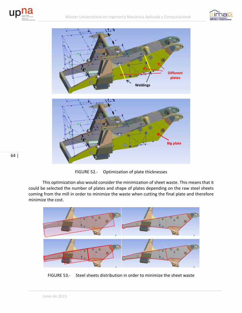
Master Universitario en Ingeniería Mecánica Aplicada y Computacional
Junio de 2015
64 |
FIGURE 52.- Optimization of plate thicknesses
This optimization also would consider the minimization of sheet waste. This means that it could be selected the number of plates and shape of plates depending on the raw steel sheets coming from the mill in order to minimize the waste when cutting the final plate and therefore minimize the cost.
FIGURE 53.- Steel sheets distribution in order to minimize the sheet waste
Different plates
Weldings
Big plate

Assessment of different optimization techniques for the structural components of a mining truck
Paula Aranzadi de Miguel
| 65
Actually, the internal wall of each of the sides is already formed by different steel sheets where thicker plates were regarded to be needed. It could be optimized the shape and size of these thicker plates. The parameters or design variables could be directly related to the geometry.
FIGURE 54.- Optimization of the shape of the steel sheets
The frame model has been previously designed in Pro/ENGINEER. The quasi-static analysis was made in Pro/MECHANICA, but the durability analysis was made with Virtual Lab Durability based on an ANSYS Workbench model.
Since Pro/MECHANICA is not a software with accessible deck files, they are encrypted and are not open, but in ANSYS the solver decks are accessible, it is going to be used the ANSYS model.
The software used for the optimization algorithm is HyperStudy in this case, which is a free solver tool in terms that can be used in conjunction with a FE solver like ANSYS. Besides, HyperStudy has an application that has been especially developed for ANSYS and all the process is adapted to find all the parameters and run the optimization analysis quickly and efficiently.
In ANSYS Workbench it is possible to define parameters for the purpose of creating a Design of Experiments or an optimization. These parameters could be geometry, properties of the elements or even responses of the system. It has to be defined as parameters both the design variables that are subjected to change and the system responses that are aimed to be monitored, both because they are part of the objective function or they are constraints that have to be accomplished.
Different plates

Master Universitario en Ingeniería Mecánica Aplicada y Computacional
Junio de 2015
66 |
FIGURE 55.- Definition of parameters in ANSYS Workbench
4.2.1 DISCRETE VARIABLES – SHELL THICKNESSES PARAMETERIZATION
According to the ideas explained at the beginning of this section, one of the parameters that could be optimized in the frame model is the thickness of the steel sheets. The steel plates of the frame are modeled with 2D shell elements. Those elements need a property that defines the thickness. This property is the parameter that is going to be set up as the design variable.
Furthermore, the weight is a parameter that has to be controlled since the objective function is going to be minimize weight of the frame.

Assessment of different optimization techniques for the structural components of a mining truck
Paula Aranzadi de Miguel
| 67
FIGURE 56.- Parametrization in ANSYS Workbench of the model Mass (objective function)
On the other hand, it has to be defined as parameters as well the stresses on the plates and castings because they are going to take part in the optimization constraints. The material is not allowed to plastic deformation, for fatigue reasons, so the boundaries of the design space of the optimization problem are going to be the yield stresses of both materials: steel and casting, each of them for the corresponding elements.
FIGURE 57.- Parameterization in ANSYS Workbench of the equivalent stress (response monitored for the optimization constraints)

Master Universitario en Ingeniería Mecánica Aplicada y Computacional
Junio de 2015
68 |
The design variables of the optimization are the thicknesses of the plates. Since the property is assigned in ANSYS Workbench through a named set, all the elements within this named set are going to have the same property. It is to say that the optimization will consist on finding the optimum thickness for the current plates, but it is not going to define the thickness distribution according to the load path in this case.
FIGURE 58.- Definition of shell thickness as parameters (design variables)
In order to make the problem affordable in terms of computational and time cost, at the beginning it is defined as design variable just the thicknesses of the walls of the sides of the frame.
There is one consideration to add, and it is that the thicknesses are not continuous variables, but discrete. It means that the thicknesses that should be considered as a possible solution should match the available thicknesses in the market.
It is important to set up the optimization problem as a discrete design space from the beginning, since depending on the nature of the problem the rounded up value of a continuous solution not always coincide with the discrete optimum solution.
4.2.2 OPTIMIZATION ALGORITHM
Within HyperStudy there are nine different optimization algorithms or engines available and they should be used depending on the nature of the problem to be solved: linear system response, non-linear system response, stationary or transient analysis, …
□ Adaptive Response Surface Method (ARSM)
□ Global Response Surface Method (GRSM)

Assessment of different optimization techniques for the structural components of a mining truck
Paula Aranzadi de Miguel
| 69
□ Sequential Quadratic Programming (SQP)
□ Method of Feasible Directions (MFD)
□ Genetic Algorithm (GA)
□ Single Loop Approach (SLA)
□ Sequential Optimization and Reliability Analysis (SORA)
□ SORA-ARSM
□ Multi-Objective Genetic Algorithm
□ Hybrid Multi-Objective Method for Optimization
□ User defined – Xopt
The first five algorithms are meant for deterministic optimizations. Next three are for robust design and the last ones are for multi-objective optimization.
It should be used the Adaptive Response Surface Method since it is the most appropriate for linear static analysis.
The project was stopped at this point for several reasons, mainly because there were found some difficulties in the talking between the two softwares: ANSYS Workbench and HyperStudy. For running the optimization HyperStudy estimates the change on the design variables according to the optimization algorithm selected, load them into the input deck file of ANSYS Workbench and then it tells ANSYS Workbench analysis to be run. After the analysis is done in ANSYS, HyperStudy reads the responses in the output file of ANSYS and determines next design variables change. It has to do these steps as many times as needed for achieving the optimum solution, and therefore no manual interaction with the user is desired, but it was not the case. In order to advance to next iteration HyperStudy needed the user to click on one bottom due to some problems that it was not possible to get rid of, and since each of the static analysis in ANSYS took more than 1h, it was not manageable to run the optimization “manually”.
4.2.3 DISCUSSION: HOW TO OPTIMIZE BASED ON DURABILITY ANALYSIS WITH VIRTUAL
LAB DURABILITY
Some discussions about future steps were made. Since HyperStudy is a solver free tool that could interact, in theory, with any other solver as long as the input and output files are accessible by a third party, and the optimization would be desired to be run based on durability analysis, it was thought to prepare a batch for the flow of the fatigue analysis.
As explained previously, the durability analysis or fatigue analysis for the truck parts is done in FALANCS or in Virtual Lab Durability (depending on the model). In case of Virtual Lab Durability, an ANSYS Workbench model is needed in the first place. It is run one unitary load case for each of the components of each of the loads (forces and moments) in the model. Then, the

Master Universitario en Ingeniería Mecánica Aplicada y Computacional
Junio de 2015
70 |
fatigue post-processor (Virtual Lab durability) is fed with the stress resulting from the unitary load cases, the material properties (curve SN) and the durability schedule, which is the combination of load cases time series and number of occurrences. The post-processing is based on the assumption of linear behavior of the part, linear relationship between stress and load. The total stress at each time can be found superimposing the stress under unitary load multiplied by the actual load component in this particular time.
After the load history is translated into a stress history, it is carried out the Rainflow Cycle Counting (RFCC) and then fatigue life of the part is calculated according to Palmgren-Miner’s Rule finding in the SN curve the allowable number of occurrences before failing under fatigue, N, and according to the number of occurrences that each particular stress range was found in the RFCC.
HyperStudy should then access HyperStudy, change the values of the design variables according to the optimization algorithm, run the unitary load analysis in ANSYS Workbench, access the results in ANSYS in order to create the input in Virtual Lab Durability, run the fatigue analysis and then read the fatigue results in HyperStudy to be able to find the change in the design variables for next iteration.
There are some difficulties in the setup of this problem. First of all, the problems found in the correlation between HyperStudy and ANSYS Workbench have to be gotten rid of. Secondly, all the process is very expensive in computational terms. For the case of the frame model, there are almost 100 load components to be applied, so it means 100 unitary load load cases to be run. Besides, the fatigue analysis is also long, so to run each of the iteration of the optimization problem will take almost one day.
It could be thought to let the software run for as much time as needed, but there are some actions that are not automatized in the fatigue analysis due to the fact that the judgment of the user is needed to take some decisions. For example, in case of weldings, the FAT CLAS.

Assessment of different optimization techniques for the structural components of a mining truck
Paula Aranzadi de Miguel
| 71
4.3 ADVANCED TOPOLOGY AND FINE-TUNING OPTIMIZATION - OPTISTRUCT
Finally, the last tool available from Altair is OptiStruct. It is the both the engine for the optimization analysis as well as the solver for the FE analysis.
The optimization types available in OptiStruct are called:
□ Topology for 3D elements
□ Topology for 2D elements
□ Topography
□ Shape
□ Size
□ Free-shape
□ Free-size
The optimization model setup is done in HyperMesh, pre-processor of Altair. If the FE model were available in any other platform, for example ANSYS, HyperMesh would be able to import the model, but maintaining ANSYS input deck cards. If optimization is the analysis aimed to be carried out, then the model will have to be translated into OptiStruct. There is one tool within HyperMesh for translating from ANSYS into OptiStruct.
The goal of this project is just to evaluate how could be introduced the optimization techniques, so the frame model created in ANSYS Workbench is going to be used instead of creating a new model from zero. It is analyzed the different optimization techniques that could be applied in the different parts of the frame model.
4.3.1 TOPOLOGY IN OPTISTRUCT
Topology optimization in OptiStruct is considered to be more advanced than in Inspire, not for the optimization algorithm itself, but for the freedom over the control of all the finite element model. Since OptiStruct is a FE solver, all the capabilities of the FE solver are available to be applied for the optimization analysis. For example it might be done non-linear analysis or even fatigue analysis.
Besides, there are two different types of topology: 3D elements topology and 2D elements topology. Topology optimization, as explained in section 3.2, hides the elements of the design space model that do not contribute to the load path. The way to hide the elements is applying to the stiffness matrix a density factor that varies between 0 and 1 and as a consequence makes the corresponding element to contribute to the total stiffness or not.

Master Universitario en Ingeniería Mecánica Aplicada y Computacional
Junio de 2015
72 |
In case of the 3D elements topology optimization the density factor is forced at the end to be 0 or 1, which means that the element is considered or not. The threshold value to force to go to 1 or 0 may be changed, but normally is setup to 0.5. All the elements which density factor is higher than 0.5 are shown, are forced to go to 1, and all the elements below 0.5 are forced to 0 and are hidden.
3D elements topology optimization is very convenient and appropriate for castings and for new design, since it is not created any restriction on shape or space in the setup of the optimization model. The design space covers all the room available for the part in design.
In case of 2D elements topology optimization, the density factor is not forced to go to 0 or 1, but is used to adjust the thickness property. All the shell elements have a predefined maximum thickness. After the 2D element topology optimization, each of the shell elements will show the adjusted thickness depending on the density factor that depends on the load path. As a conclusion, the 2D elements topology optimization could be understood as an optimization of the thicknesses of each of the shell elements in the problem. It is different from the parametric optimization explained in section 4.2.1, because in that case the design variable was the thickness of the property of the element, so all the elements sharing same property are conditioned to have same thickness. If each of the shell elements are aimed to be optimized, then it is needed one different property for each of them. In case of the topology optimization, just one property could be assigned to all the elements for the optimization analysis, because the design variable is not the thickness of the property, but the density factor that applies to each element representing its contribution to the load path.
This kind of optimization is appropriate when it is known ahead of time that the part is going to consists of steel plates. The 2D topology optimization will give in return the optimized thickness distribution along the plate. It is up to the designer or analyst to decide where to cut each of the plates, because there are more factors to consider like for example the welds between the plates. Once the plates distribution is decided, a parametric optimization (called size optimization in OptiStruct, explained later) of the thickness property of each of the plates will be necessary to adjust them.
4.3.2 TOPOGRAPHY OPTIMIZATION
Topography optimization was developed specially for parts manufactured by form-pressing or stamping. It is aimed to be used over 2D elements, but in this case the thickness property remains constant and the design variables is the position of the nodes in the perpendicular direction of the plane 2D. The optimization will drop the distribution and shape of beads to stamp over the plate making it stiffer.

Assessment of different optimization techniques for the structural components of a mining truck
Paula Aranzadi de Miguel
| 73
FIGURE 59.- Example of topography optimization on a container
Topography optimization is not considered at this point for the frame model since there is not stamping in it.
4.3.3 SHAPE OPTIMIZATION
Shape optimization has for design variables the position of the nodes of certain area of the mesh. This technique is also known as morphing. The movement of the nodes has to be defined by means of vectors giving the direction. The definition of this vectors in OptiStruct are very different, including from modifications of geometry dimensions to directions defined by a modal analysis or a user defined direction. The great advantage of morphing in OptiStruct, called HyperMorph, is that the changes are done without remeshing the model. This fact makes easier the assessment of the analyst since the comparison between original and optimized solution is straight forward (same nodes, same elements that have to be evaluated).
FIGURE 60.- Example of shape optimization that helps to relieve stress concentrations around holes
Shape optimization could be applied in different parts of the frame model. Firstly, for the definition of the position of the internal reinforcement (vertical ribs) that are allocated inside the two walls that form each of the sides of the frame. Furthermore, those reinforcements consist of

Master Universitario en Ingeniería Mecánica Aplicada y Computacional
Junio de 2015
74 |
plates with some internal holes. The size and shape of the holes could be optimized too using shape optimization.
FIGURE 61.- Optimization of frame walls internal reinforcement position
Secondly, there are some welding windows made on the walls of the frame sides, precisely in order to be able to weld the reinforcement inside the walls. The shape in these windows could be optimized (both the position and the size) using shape optimization.
On the other hand, the 2D topology optimization was claimed to be adequate to find the distribution of thicknesses, and as a consequence the distribution of different plates and welds between the plates. Once the analyst judges the best distribution of plates, it could be “fine-tuned” the position of this separation. In this case just slightly changes will be done during the optimization analysis with the purpose of finding the orientation and best position of the welds according to fatigue calculations. Shape optimization would find those best positions.
4.3.4 SIZE OPTIMIZATION
In size optimization the design variables are the properties of the elements of the model. For example, the thickness of the shell properties, the cross-section of a 1D element, the stiffness of a spring, …
This kind of optimization, as previously claimed, is adequate to find the optimized thickness of the steel plates that forms the frame. It is presupposed that the plates shape is known, and the only design variable eligible to be changed is the thickness of each of the plates.
Stiffeners inside walls
Optimization of position of the internal reinforcement ribs

Assessment of different optimization techniques for the structural components of a mining truck
Paula Aranzadi de Miguel
| 75
4.3.5 FREE-SIZING
There is a particular type of optimization related to size in OptiStruct called Free-Sizing. This optimization technique is for composited, in which not just the element property (thickness) is the design variable, but also the direction of the material property (defining fiber orientations in the composite material). For this reason, it is no applicable at this point in the frame model of the truck in study.
4.3.6 FREE-SHAPE
This last optimization, free-shape, belongs to the group named “fine-tuning” with shape, Size and free-size. The term “fine-tuning” means that the geometry is subjected to slightly changes that are going to give the user almost the final design.
In particular free-shape optimization is used for relieving stress concentrations at certain areas of the part, like fillets or in the surroundings of holes. Also after carrying out a 3D topology optimization it would be interesting to run a free-shape optimization in order to relieve high stresses in the connections between design space and non-design space like the ones saw in the optimization of the control arm in Inspire.
However, it is important to have always in mind that this optimization should be used just at the end of the design where little changes in the shape should be expected. The reason is that, unlike the shape optimization, in this case all the nodes in the designed area are free to move in whatever direction. It could be set up the just in one direction, but the idea is that in this case there are not constraints between the nodes, in the relative movement of the nodes. It is defined a frontier, upper and lower limit, that should not be exceeded, but it is an expensive solution in computational terms though.
4.3.7 ANSYS FRAME MODEL
It is possible to import in HyperMesh a classic ANSYS model, so first thing done is convert the ANSYS Workbench model into a cdb file, classic ANSYS model.
Once the model is loaded in HyperMesh, in order to be able to carry out an optimization analysis in OptiStruct, it has to be translated from ANSYS into OptiStruct. Most of the setup of the model is easy to translate since the element definition is similar in both solvers, just the nomenclature changes.
However, there are some features in ANSYS that are not supported in OptiStruct, so it is not direct to translate. One of these features is the definition of the load cases through tables. The frame model in ANSYS has 35 load application points. Each of these application points has 3 load components, so it makes a total of 105 loads. For optimization purposes, similar to the case of the control arm, it is really important to consider all the load situations that could happen

Master Universitario en Ingeniería Mecánica Aplicada y Computacional
Junio de 2015
76 |
during the whole life of the frame. In this case the ultimate loads table, which represent the extreme load envelope, is reduced to 9 different load cases.
In order to be able to define in ANSYS Workbench the 9 load cases in the same model it has to be done by means of a load table. In this load table, each of the rows represents a load step which is one of the extreme load case, so the table has 9 rows in total. To sum up, the model has 25 load application points, and each of the loads is defined in a table which has 3 columns for the 3 components of the load and 9 rows for each of the load cases.
When it is translated the ANSYS model into OptiStruct, Altair’s software is not able to relate the tables to the loads at this point, and it misses all the load information.
Since the final goal of this project was not to optimize the frame itself, but evaluate and research the different techniques for optimization based on FEA, and considering that in order to be able to run the analysis on the frame model more time is required to setup everything correctly, it is decided to stop the project here. Future steps will be:
□ Work with Altair in the conversion from ANSYS to OptiStruct model or re-build a whole complete frame model in OptiStruct;
□ Run topology 2D optimization on all the steel sheets in order to find the optimized shell thickness distribution;
□ Decide how to split the steel sheets considering other facts besides the thickness distribution given by the topology optimization, like the manufacturability of the steel plates or the quantity of welds and of course the final cost;
□ Run a size optimization over the thickness property of the plates decided in previous step;
□ Run a shape optimization on the position of the welds between plates;
□ Run a shape optimization on the position of the internal reinforcement ribs of the sides of the frame;
□ Run a 3D topology optimization on the castings of the frame, which are the connectors between the two sides basically;
□ Run a free-shape optimization in order to relieve stress concentrations where needed. Typically run after a 3D topology optimization.

Assessment of different optimization techniques for the structural components of a mining truck
Paula Aranzadi de Miguel
| 77
5 CONCLUSIONS
There are two different points about which state some conclusions. First of all about the different optimization techniques and how to introduce them, and secondly about the software assessed for this purpose of optimization.
5.1 CONCLUSIONS ABOUT THE DIFFERENT OPTIMIZATION TECHNIQUES BASED
ON FEA
Depending on the part that is aimed to be optimized, the manufacturing process and how is it modeled in FE analysis, one optimization technique (based on FEA) should be used or another.
For castings, topology optimization seems to be the most appropriate, since there is more freedom in terms of the shape of the geometry, and the optimum solution would be the load path within the design space considering it as all the room available in the assembly. In this case the design variables are the densities of the elements that multiply the stiffness matrix. The value of the densities represent the contribution of each of the elements to the load path and therefore the optimized geometry is the contour of the elements which density is above the safety factor considered.
After the topology optimization, it could be necessary to do some fine tune optimization. For that, free-shape optimization would be the most appropriate. In the free-shape optimization it is defined a set of nodes that could move in any pre-defined direction within certain limits. This optimization technique will help to relieve high stresses that could appear in the model because of the translation of the topology concept design into real and manufacturable geometry.
For parts made of steel sheets, different optimization techniques could be used in combination. First of all, a 2D elements topology optimization would give the optimized thickness distribution along all the part. According to this thickness distribution, a judgment on how many plates to use considering the sheet waste and the number of welds could be made. After deciding the number of plates and the size of them, a thickness optimization of each of the sheets should be done in order to find for the final plates distribution the appropriate thickness. As well a fine tune optimization of the shape or exactly position of the cuts of the sheets could be done with free size optimization. This last optimization would be ideally done based on fatigue on the welds.

Master Universitario en Ingeniería Mecánica Aplicada y Computacional
Junio de 2015
78 |
5.2 CONCLUSION ABOUT ALTAIR SOFTWARE FOR OPTIMIZATION
The software offered by Altair for optimization purposes could be divided in two different groups: SolidThinking and HyperWorks. Inspire, which is the simplified topology optimization tool belongs to SolidThinking side and OptiStruct and HyperStudy to HyperWorks.
Inspire SolidThinking is a tool that can be used separately from all HyperWorks environment. It is simple to use and designer friendly. It means that it is not needed a deep knowledge in FE analysis in order to be able to use it. However, it is also quite limited in terms of analysis because the user do not have too much control over the finite element properties. If used adequately (considering all loading scenario, representing correctly the behavior of the part, defining correctly the design space for avoiding interferences in the final assembly, …) it is considered a good tool to help the designer to achieve a good and optimum solution of the part faster than in a conventional way based on trial and error. This is because the topology optimization gives a design concept based on the load path. This conclusion has been proven in the optimization of the control arm using Inpsire, where despite the fact that the part had gone through a long process of re-design along the years, 55kg (8% of the total weight of the part) has been reduced. If this technique is used from the beginning of the creation of a new part, the savings in cost and time will increase.
The rest of the HyperWorks software is very complete and gives the analysis and simulation engineer a wide range of optimization techniques that covers from topology optimization to fine tune analysis. Besides HyperStudy could be used in combination with a third party software, but, it has been found some difficulties. For fatigue based optimization, it is quite expensive in terms of time and computation, so it is theoretically adequate, but practically is not very easy to implement. The utilization found for the truck parts during this project of HyperStudy, i.e. shell thicknesses optimization, could be also be performed in ANSYS Workbench.
OptiStruct uses for the shape and size optimization all the power of HyperMorph and HyperMesh in order to maintain a good mesh when it is changed in the optimization process, and in order to make the most of the software it should be used in conjunction with the rest of the environment of HyperWorks. It is theoretically possible to translate for example an ANSYS model into OptiStruct, but the ideal situation would be to work directly in OptiStruct and build the model in it for making the most of the software.
Then, in order to come up with a conclusion, it makes sense to use OptiStruct and HyperStudy if all the analysis tools are going to be migrated into HyperWorks environment. If it is desired to keep on working using Pro/MECHANICA, ANSYS, …, it is arguable the suitability of the software just for optimization purposes. It is not straight forward to translate the model into OptiStruct, so a huge work load is needed for the setup of the model again, and the licenses are quite expensive.

Assessment of different optimization techniques for the structural components of a mining truck
Paula Aranzadi de Miguel
| 79
6 BIBLIOGRAPHIC REFERENCES
[1] “Structural Optimization using OptiStruct. Concepts, Analysis, and Optimization for General Structures.” Altair 2014.
[2] “HyperStudy Introduction. DoE, Fit, Optimization and Stochastic”. Altair 2014.
[3] Apuntes de la asignatura “Elementos finitos II” impartida por Jesús Zurita Gabasa en el curso académico 2010-2011 en el Máster de Ingeniería Mecánica Aplicada y Computacional en la UPNA.
[4] Apuntes de la asignatura “Fatiga de Componentes y Estructuras” impartida por Fco. Javier García Zabalegui e Isidro Zabalza Villava en el curso académico 2011-2012 en el Máster en Ingeniería Mecánica Aplicada y Computacional en la UPNA.
[5] “Structural optimization in FE analysis”. NAFEMS, online training documentation, February 2015.
[6] “Fatigue Equivalent Load Cycle Method”. H.B. Hendricks and B.H. Bulder, October 1995. ECN-C-95-074
Copyright © 2022 FDOKUMEN