Assessing Suitable and Critical Habitat for Wood Bison (Bison bison athabascae) Using Geographic...

Assessing Suitable and Critical Habitat for Wood Bison (Bison bison athabascae) Using Geographic Information Systems (GIS) and Remote Sensing: Preliminary Results OLAF C. JENSEN1, JOHN NISHI2, NORM L. COOL3, DAVID POLL4, AND HAL W. REYNOLDS1

1Canadian Wildlife Service, Room 200, 4999 98 Avenue, Edmonton, AB, T6B 2X3, Canada, email [email protected], Wildlife and Economic Development, Government of the Northwest Territories, Fort Smith, NT, X0E 0P0, Canada 3Elk Island National Park, Site 4 RR1 Fort Saskatchewan, AB, T8L 2N7, Canada 4Parks Canada, Room 550, 220 4th Avenue SE, Calgary, AB, T2G 4X3, Canada Abstract: The wood bison (Bison bison athabascae)1 is currently listed by the Committee on the Status of Endangered Wildlife in Canada (COSEWIC) as a nationally threatened species. The principal goal of the National Recovery Plan for the Wood Bison is “to foster the recovery of wood bison in other parts of their original range and in suitable habitat elsewhere, thereby ensuring their long term survival.” This recognition of the importance of habitat conservation, along with the requirement of the Canadian Species at Risk Act that habitat and critical habitat for listed species be identified in recovery strategies and/or action plans, necessitates an objective definition of critical habitat for wood bison. Definitions of suitable and critical habitat can be addressed at different spatial scales. We present a method of assessing resource selection when resources are considered simultaneously at multiple spatial scales. Specifically, we assessed habitat selection by wood bison at the landscape scale using a Geographic Information System (GIS) and remote sensing-derived data because this is the scale at which most management decisions will likely be made. We evaluated bison habitat use from aerial survey and radio-telemetry data within Wood Buffalo National Park, the adjacent Slave River Lowlands, and the Mackenzie Bison Sanctuary. We assessed resource selection function models using Akaike information criteria to model landscape resource selection, and used Landsat-derived vegetation data, soils data, and various landscape metrics to assess selection of habitat types within the landscape. We suggest that habitat, by its definition, is suitable. Further, the concept of critical habitat for wood bison is inextricable from the population goals of recovery, thus necessitating population viability analysis. Models and information that flow from this work will be used in future considerations and assessments of potential reintroduction sites. Key Words: wood bison, Bison bison athabascae, Bos bison athabascae, habitat, GIS, Geographic Information System, resource selection function, Akaike information criteria, Wood Buffalo National Park, Mackenzie Bison Sanctuary, Slave River Lowlands, Alberta, Northwest Territories

1NatureServe Explorer (version 4.0, July 2004) lists the wood bison as Bos bison athabascae. T.D. Hooper, editor. Proceedings of the Species at Risk 2004 Pathways to Recovery Conference. 1 March 2–6, 2004, Victoria, B.C. Species at Risk 2004 Pathways to Recovery Conference Organizing Committee, Victoria, B.C.

mailto:[email protected]

Critical Habitat for Wood Bison Jensen et al.

Introduction

The wood bison (Bison bison athabascae) is the largest grazing ungulate in the boreal forest. Concurrent with the demise of the plains bison (Bison bison bison), the wood bison population decreased to an estimated low of < 250 animals. Protection efforts in the early 20th century, including the establishment of Wood Buffalo National Park in 1922, coincided with an increase in wood bison to approximately 1500 animals; however, this initial recovery was irrevocably affected by the Government of Canada’s decision to move more than 6000 plains bison into Wood Buffalo National Park from 1925 to 1928 (Fuller 2002). The translocation introduced plains bison genes, and cattle diseases—bovine tuberculosis (Mycobacterium bovis) and brucellosis (Brucella abortus)—into the native wood bison population. Introgression of plains bison genes was widespread, and the Wood Buffalo National Park bison population remains enzootic with the two cattle diseases. The discovery of a small, isolated herd of wood bison in the Nyarling River range in northwestern Wood Buffalo National Park in 1957 precipitated conservation efforts in the 1960s that resulted in the establishment of the Mackenzie Bison Sanctuary and the Elk Island National Park wood bison herds. Both herds are considered to be free of bovine tuberculosis and brucellosis. Current Recovery Efforts

The wood bison is listed as Threatened by the Committee on the Status of Endangered Wildlife in Canada (COSEWIC 2001), and a recovery team has been established. The principal goal of the National Wood Bison Recovery Plan (Gates et al. 2001) is “to foster the recovery of wood bison in other parts of their original range and in suitable habitat elsewhere, thereby ensuring their long term survival.” A specific objective of the plan is to establish a minimum of four free-roaming, disease-free herds of at least 400 animals each (Gates et al. 2001). A definition of critical habitat in the context of wood bison is inseparable from these population goals. In concert with these requirements, the Species at Risk Act (SARA), which was proclaimed on 5 June 2003, requires that habitat and critical habitat for listed species be identified in recovery strategies and/or action plans. Resource Selection

Resource selection takes place within a hierarchy of spatial scales (Johnson 1980). On the smallest spatial scale, bison select slough sedge (Carex atherodes), seasonally select northern reedgrass (Calamagrostis canadensis), and at another spatial scale, select meadows dominated by these plants (Reynolds et al. 1978; Larter and Gates 1991; Fortin et al. 2002). Meadow selection comprises third-order selection and includes use of other vegetation communities including deciduous forests, which are used for resting, ruminating, and avoiding biting flies (Reynolds et

Proc. Species at Risk 2004 Pathways to Recovery Conference. 2 March 2–6, 2004, Victoria, B.C.


al. 1978). Additionally, the selection of patches within a landscape is influenced by such factors as distance to water (Fortin et al. 2003), patch size (Reynolds et al. 1978), and type of vegetation community found proximate to a patch of forage habitat.

At the two smallest scales, resource selection is active: an individual or group makes decisions about what plant it consumes and in what patch it will do so. Resource selection at this scale follows an energy maximization strategy (Bergman et al. 2001), and a simple gain function determines the value of a patch (Stephens and Krebs 1986). At larger scales, bison behave as time-minimizers since their foraging behavior is constrained by biting flies, predation risk, and movement decisions made by the herd, to name but a few. Not withstanding these conflicting demands, long-term average rate-maximizing is the goal if an individual is to maximize its fitness (Stephens and Krebs 1986). Persistence in a landscape and passive resource selection depends on a landscape containing the necessary forage resources and landscape covariates if an individual is to maximize its fitness over the long term. The marginal value theorem is one way to conceptualize and model the landscape metrics that might lead to increased fitness and persistence. The marginal value theorem predicts that forage patches must necessarily increase in size and/or quality in relation to how distant they are from other forage patches. Energy lost in travel through the landscape matrix must be recovered in forage patches.

Some constraints on active resource selection include predation (Carbyn et al. 1998), biting flies (Bergman et al. 2001; Fortin et al. 2003), distance to water (Fortin et al. 2003), and in winter, aeolian snow hardening and snow depth (Reynolds et al. 1978; Fortin et al. 2003). The quality of the environment surrounding forage habitat and the travel costs associated with movement through the matrix in which forage habitat is embedded will affect dispersal and survival of a population of animals (Bender et al. 2003). Study Area

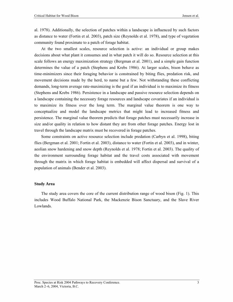
The study area covers the core of the current distribution range of wood bison (Fig. 1). This includes Wood Buffalo National Park, the Mackenzie Bison Sanctuary, and the Slave River Lowlands.



Figure 1. Study area showing the approximate distribution of wood bison (grey lines). Methods

Resource selection can be assessed with numerous statistical tools, including selectivity indices and a resource selection function (RSF). Selectivity indices compare the proportion of used habitat to the proportion available to test whether habitats are used disproportionately to their availability. Selection can be statistically assessed in this manner and preference for certain habitat types can be measured. An RSF is created from an analysis of the data and is directly related to the probability that a given resource will be used by an animal (Boyce and McDonald 1999). Resource selection and probability functions can be used to generate maps of probability of use within a landscape; these in turn can be used to identify suitable habitat. A probability-of- use map generated from a resource selection probability function is essentially a habitat suitability index (HSI) map, but with statistical rigor (Boyce et al. 2002).

In this study, we considered resources to be communities of vegetation called ecosites, which are ecological communities defined as “a plant community of definite floristic composition, uniform habitat condition and uniform physiognomy” (Ponomarenko and Alvo 2001). We created a unified digital resource map for the study area from a hierarchal unsupervised ISOCLUS (Iterative Self-Organizing Clustering algorithm) classification of Landsat imagery (Jensen and



Sánchez-Azofeifa, in press). A hierarchal classification scheme was developed from an element-based phytotopological ecosystem classification scheme that was developed for the area (Beckingham and Archibald 1996), and these ecosites were considered to be resources in our study. We aggregated the final classification to a 12-class digital map with a minimum mapping unit of 1 ha. Model covariates (Table 1) were obtained in the following manner: elevation and terrain ruggedness were created from a 1:50 000 digital elevation model; all other metrics were generated using FRAGSTATS (Version 3.3), a grid-based program for calculating landscape metrics (McGarigal et al. 2002). These landscape metrics were calculated using a circular moving-window analysis with a radius of 2 km on the resource map described above. We set the size of this landscape equal to the daily movement of a bison (Fortin et al. 2003). The value of each metric is returned to the cell at the center of the window, so each metric is a measure of the local landscape, measured at a scale relevant to a bison. Variable and covariate values were assigned to each observation and relocation. Used locations were defined as those sites in the database relating to an actual occurrence of a bison—these include aerial survey and telemetry relocation points. Available points were collected randomly along a uniform distribution within each population’s range and again over the entire study area for a total of 20,000 points. Standard errors for selected variables were assessed in relation to increasing sample size of random available points. We followed King and Zeng’s (2000) recommendation for selecting sample sizes for available points, which was 2–5 times the number of used points. Table 1. Model variables and covariates used in resource selection function (RSF) modeling.

Code Covariate name Description

Classification variables ID Observation ID From bison observation database Easting X location Easting in UTM NAD 83 Zone 12 Northing Y location Northing in UTM NAD 83 Zone 12 Used Used Used or available location Type Type of point Random, telemetry or aerial survey point Bison Bison ID Taken from field data tables Group Population Population to which the individual is assumed to belong GrpSize Group size Observed group size at time of relocation Season Season Season of observation

Patch variables (active selection) Eco12 Land Cover Class 12 class Ecological Land Cover Perimeter Perimeter Patch perimeter Area Patch area Total size of the patch, regardless of landscape size Fractal Fractal dimension Patch fractal dimension Rugged Terrain ruggedness index Local topographic variation derived from a 1:50 000

Digital Elevation Model (DEM)



Table 1. Model variables and covariates used in resource selection function (RSF) modeling (cont’d).

Code Covariate name Description

Local landscape variables (active passive selection) Elev Elevation Elevation derived from 1:50 000 DEM CONTAG Contagion Measure of landscape homogeneity CWED Contrast weighted edge

density Quantity of edge for each landscape, weighted by type

ED Edge density Unweighted measure of edge density DW Distance to water Distance to nearest water source SIDI Simpson's index of

diversity Measure of landscape diversity

Per1-12 Percentage Percentage of cells within 300 m buffer around points Ca1-12 Class area Class area for each class in the landscape Clumpy1-7,9 Clumpiness Measure of the proximity of similar patch types CWED1-7,9 Contrast weighted edge

density Weighted edge density for each patch type

Enn1-7,9 Euclidean nearest neighbour

Straight-line distance to patch of same class

Frac1-7,12 Fractal dimension Measure of complexity of local landscape IJI1,3-7,12 Interspersion

juxtaposition index Interspersion for class type

PD1-7,9,12 Patch density Patch density for each class type Teci1-6,12 Total edge contrast index Calculated for each class within the landscape IJI Interspersion

juxtaposition index Measure of landscape homogeneity

Landscape variables (passive selection) SC Soil class Slave River Lowlands soil class from 1974 survey

Telemetry data were generously provided by Joly and Messier (2001, unpublished results collected as part of a disease study conducted in Wood Buffalo Nation Park, 1998–2000); Wood Buffalo National Park (unpublished results from a movement and distribution study initiated in 1998); and the Mackenzie Bison Sanctuary (Larter 1998). Aerial survey data were obtained for the Mackenzie Bison Sanctuary, Slave River Lowlands, and Wood Buffalo National Park from the Department of Resources, Wildlife and Economic Development (RWED), the Government of the Northwest Territories, and Wood Buffalo National Park, respectively.

We used agglomerative hierarchal clustering (Podani 2001) to delineate populations of bison in the study area using median seasonal locations of each collared bison in the population (Joly and Messier 2001; Taylor et al. 2001). Populations were defined as being spatially, genetically, or demographically disjunct groups of animals, and metapopulations were understood to be disjunct groups with some demographic or genetic connection (Wells and Richmond 1995). We identified five distinct populations within the Wood Buffalo National Park metapopulation: Delta, Hay Camp, Garden River, Little Buffalo, and Nyarling (Fig. 1). We calculated seasonal home ranges for each bison where n > 20 using the 95% fixed-kernel home range method. Annual home ranges



were calculated from the overlay of these seasonal ranges, and population boundaries were delineated from the overlay of all seasonal home ranges for bison assigned to each population.

We used selectivity indices to test the hypothesis that resources are used disproportionately to availability, and more specifically, to examine which resources were used more than others. A Chi-square test of resource selection was used to make preliminary assessments of habitat use (Neu et al. 1976). Used habitat was determined by counting the number of cells of each habitat type contained in a 300 m buffer around each telemetry location and registering the modal value as the used habitat type. Available habitat was first compared to the vegetation communities found in the entire study area, which is ecologically arbitrary and conforms to the boundaries of the Landsat scenes used to derive the classification (Table 2). Secondly, available habitat was delineated within a polygon encompassing all observations buffered to a distance of 12 km (Table 3). This distance is equal to the average distance between telemetry relocations in Wood Buffalo National Park’s study, and is considered to be biologically relevant.

Resource variables and covariates for logistic regression were collected in a similar manner as the data used for the selectivity indices. To account for spatial inaccuracies created from telemetry relocation, we described resource variables as the percentage of each land cover class within a 300 m buffer around each relocation (Samuel and Kenow 1992; Erickson et al. 1998). Twelve biologically plausible models were created and assessed using Akaike information criteria (AIC) coefficients generated from full-model logistic regression in SAS (SAS for Windows Version 8.02). Logistic regression models were run on the full dataset, and on subsets of the data grouped by season and population, and in the case of aerial survey data, by observed group size. We demarcated seasons according to Carbyn et al. (1993). The AIC weights for the intercept and covariates were used to identify the three best models in each subset.


Critical Habitat for Wood Bisons Jensen et al.

Table 2. Habitat use by wood bison, comparing the modal value of habitat within a 300-m buffer around telemetry points to total habitat in the study area.

Habitat class No. of hectares Proportion of hectares

Observed Expected Proportionobserved

Confidence intervals Use

n = 15

lower upper significant?a

Non-vegetated 15,304.09 0.0018 25 13 0.0034 0.0016 0.0053 FALSEAnthropogenic

45,623.11 0.0055 0 40 0.0000 0.0000 0.0000 TRUE avoidBurn 351,844.69 0.0422 226 307 0.0310 0.0255 0.0365 TRUE avoidBlack spruce

615,365.15 0.0738 146 537 0.0200 0.0156 0.0245 TRUE avoid

Jack pine 1,031,302.13 0.1236 1179 901 0.1618 0.1501 0.1736 TRUE selectWhite spruce

922,303.46 0.1106 538 805 0.0739 0.0655 0.0822 TRUE avoid

Deciduous 1,207,096.50 0.1447 1207 1054 0.1657 0.1538 0.1775 TRUE selectDeciduous dominated 832,242.07 0.0998 587 727 0.0806 0.0719 0.0893 TRUE avoidShrubby poor fen 530,151.43 0.0635 80 463 0.0110 0.0077 0.0143 TRUE avoid Shrubby rich fen 1,057,392.98 0.1267 1126 923 0.1546 0.1430 0.1661 TRUE selectGraminoid fen

609,619.21 0.0731 1806 532 0.2479 0.2341 0.2617 TRUE select

Wetland 106,961.63 0.0128 135 93 0.0185 0.0142 0.0228 TRUE selectTreed bog 259,522.73 0.0311 39 227 0.0054 0.0030 0.0077 TRUE avoidTreed poor fen 596,317.64 0.0715 188 521 0.0258 0.0208 0.0309 TRUE avoid Shrubby bog 161,603.39 0.0194 3 141 0.0004 -0.0002 0.0011 TRUE avoid

Total 8,342,650.21 1.00 7285 7285 1.0000 aα = 0.05



Table 3. Habitat use by wood bison, comparing the modal value of habitat within a 300-m buffer of telemetry relocations to habitat within a narrower study area, a 12 km buffer around all telemetry relocations and aerial survey observations in the database.

Habitat class No. of hectares Proportion of hectares

Observed Expected Proportion observed

Confidence intervals Use

n = 15

lower upper significant?a

Non-vegetated 28,606.71 0.0068 159 50 0.0218 0.0172 0.0265 TRUE selectAnthropogenic

3526.63 0.0008 0 6 0.0000 0.0000 0.0000 TRUE avoidBurn 59,541.99 0.0142 226 104 0.0310 0.0255 0.0365 TRUE selectBlack spruce 323,538.99 0.0774 146 564 0.0200 0.0156 0.0245 TRUE avoid Jack pine 626,198.86 0.1498 1179 1091 0.1618 0.1501 0.1736 TRUE select White spruce 501,365.86 0.1200 538 874 0.0739 0.0655 0.0822 TRUE avoid Deciduous 580,712.86 0.1389 1207 1012 0.1657 0.1538 0.1775 TRUE selectDeciduous dominated 440,268.82 0.1053 587 767 0.0806 0.0719 0.0893 TRUE avoid Shrubby poor fen 99,466.84 0.0238 80 173 0.0110 0.0077 0.0143 TRUE avoid Shrubby rich fen 625,917.01 0.1497 1126 1091 0.1546 0.1430 0.1661 FALSE Graminoid fen 472,413.78 0.1130 1806

823 0.2479 0.2341 0.2617 TRUE select

Wetland 82,578.78 0.0198 1 144 0.0001 -0.0002 0.0005 TRUE avoidTreed bog 81,321.09 0.0195 39 142 0.0054 0.0030 0.0077 TRUE avoid Treed poor fen 218,710.50 0.0523 188 381 0.0258 0.0208 0.0309 TRUE avoid Shrubby bog 35,597.67 0.0085 3 62 0.0004 -0.0002 0.0011 TRUE avoid

Total 4,179,766.37 1.0000 7285 7285 1.0000 aα = 0.05



Results

With roughly 200 points, variance stabilized at < 1 SE (Fig. 2). Approximately 18,500 available locations, 7700 telemetry relocations, and 9500 aerial survey observations were included in the analysis. For any statistical test of resource selection using logistic regression, we rejected tests, regardless of the results, where the number of available locations was less than 200.

0

1

2

3

4

5

6

7

10 20 40 100 200 400 800 1500 5000 10000 15000 20000

N (random samples)

Stan

dard

err

or

Contagion CWED Interspersion Percent grass

Figure 2. Size of the sample of available locations and its effect on the coefficient of variation for selected resource covariates. Taken from a database measures of variables at random locations (n = 19,299). CWED refers to contrast weighted edge density, as explained in the text.

Chi-square selectivity indices using Bonferroni adjustments determined consistent and significant selection for graminoid fens, deciduous forests, and occasionally, jack pine forests. Significant avoidance of bogs, conifer-dominated forests, deciduous-dominated forests, treed poor fens, and shrubby poor fens was consistently recorded (P < 0.05; Tables 2 and 3). Selection changed as definitions of availability changed. Most significantly, shrubby rich fens were significantly selected when availability was determined as the entire study area, which is ecologically arbitrary. When availability was defined using more biologically relevant criteria within a buffer of all telemetry relocations, selection for shrubby rich fens was not significant. Also, recently burned areas were avoided when availability was measured over the entire landscape, but were selected for within the narrower, more biologically relevant landscape.



Of the twelve models created from resource selection functions using full-model logistic regression in SAS, the best three models were as follows:

= eco12(1-7,12) + PA + CWED + PD2,4,5,6 + TRI + DW = eco12(1-7,12) + PA + CWED + PD2,4,5,6 + CONTAG + IJI = eco12(1-7,12) + PA + CWED + CONTAG + SIDI

where ecol12 = land cover class, PA = patch area, CWED = contrast weighted edge density, PD = patch density, TRI = terrain rugged index, DW = distance to water, CONTAG = contagion, IJI = interspersion and juxtaposition index, and SIDI = Simpson’s diversity index.

Ecosites within a 300 m buffer around telemetry relocations were consistently significant; deciduous forests, jack pine forests, shrubby rich fens, and graminoid fens were generally associated with positive beta coefficients (selection, not avoidance). Bog and conifer classes were generally associated with negative beta coefficients. Patch area was generally found to be significant. Contrast weighted edge density was a very strong predictor of use. It is a measure of friction within the landscape, measured within a 2 km moving window as discussed in the methods sections. FRAGSTATS (Version 3.3) counts the number of edges within the landscape, weights them according to a pre-defined weighting matrix (Table 4), and assigns a value to the center cell, which is a measure of the amount of friction or edge contrast in the landscape. A value of zero would imply no friction or edge contrast in the landscape whereas a value of one would imply that no movement is possible, or the costs of movement in this high-contrast landscape are very high. Weighting criteria were established a priori based on a review of the literature and on assumptions of how bison were likely to perceive the landscape based on their foraging needs and locomotion restrictions. Patch density was also consistently significant. Patch density is a percentage expression of the quantity of each ecosite available within the landscape or within a day’s travel of a bison from any given point. Patch densities of conifer (class 2) and bog (class 4) were consistently negative predictors of use, whereas patch densities of forage habitat—shrubby rich fens (class 5), and grass fens (class 6)—were consistently positive predictors of use. Terrain ruggedness, a local measure of topographic change interpolated from a 1:50 000 digital elevation model (DEM) was a useful metric as was distance to water, measured in meters. Contagion, the interspersion and juxtaposition index, and Simpson’s index of land cover diversity were consistently significant.



Table 4. Weights applied to the resource matrix in order to create a contrast-weighted edge density grid. A weight of zero implies no contrast between edges, whereas a weight of one implies maximum contrast.

Jack pine

Conifer

Deciduous

Bog

Shrub fen

Grass fen

Wetland

Nonveg

Water

Anthro

No data

Burn

1 2 3 4 5 6 7 8 9 10 11 12

Jack pine 1 0 0.4 0.1 0.8 0.7 0 0.5 0.3 0.9 0.4 0.0 0.2 Conifer 2 0.4 0 0 0.4 0.2 0 0.2 0.1 0.8 0.1 0.0 0 Deciduous 3 0.1 0 0 0.8 0.1 0 0.8 0.7 0.9 0.2 0.0 0.2 Bog 4 0.8 0.4 0.8 0 0.5 0.7 0.5 0.2 1.0 0.5 0.0 0.3 Shrub fen 5 0.7 0.2 0.1 0.5 0 0.1 0.5 0.4 0.8 0.3 0.0 0.2 Grass fen 6 0 0 0 0.7 0.1 0 0.4 0.1 0.7 0.2 0.0 0.1 Wetland 7 0.5 0.2 0.8 0.5 0.5 0.4 0 0.1 0.3 0.1 0.0 0.2 Nonveg 8 0.3 0.1 0.7 0.2 0.4 0.1 0.1 0 0.8 0.1 0.0 0.1 Water 9 0.9 0.8 0.9 1.0 0.8 0.7 0.3 0.8 0 0.1 0.0 0 Anthro 10 0.4 0.1 0.2 0.5 0.3 0.2 0.1 0.1 0.1 0 0.0 0.1 No data 11 0.0 0.0 0.0 0.0 0.0 0.0 0.0 0.0 0.0 0.0 0 0.0 Burn 12 0.2 0 0.2 0.3 0.2 0.1 0.2 0.1 0.0 0.1 0.0 0

Discussion

Bison select landscapes that contain a high proportion of graminoid fens (Carex spp. and Calamagrostis spp.), and use these habitats disproportionately to their availability. The results from selectivity indices suggest that at the landscape scale, bison select jack pine forests, deciduous forests, and shrubby and graminoid fens disproportionately to their availability. Shrubby and graminoid fens are selected as forage habitat. Selection for these ecosites is supported by the literature, specifically Reynolds et al. (1978), Larter (1988), and Larter and Gates (1991), who refer to shrubby fens as ‘willow-savanna’. Wetlands are also selected since they contain forage species, but these species are available only seasonally or episodically. The reasons for the selection of jack pine and deciduous forests are unclear, but these community types may be used for resting, ruminating, and escaping biting insects. Use of jack pine forests was noted by Larter (1988), who observed bison foraging on lichens in jack pine forests in the fall. Further, deciduous forests are used by some ungulates in the fall for leaf foraging, since leaves are a readily available bulking agent for ruminants (Hudson and Frank 1987).

Within the narrower landscape, delineated by a buffer of 12 km around all telemetry and aerial survey relocations in the database, bison do not select for shrubby rich fens (willow-savanna [sic, Larter and Gates 1991]) but use it in proportion to its availability. This finding suggests that bison select or persist in landscapes that contain proportionally more hectares of forage habitat, which includes shrubby rich fens, but inside of these selected landscapes they prefer forage habitat such as graminoid fens, which may be inferred to be of a higher quality since



they contain proportionally more forage than shrubby rich fens. Shrubby rich fens likely occur in higher proportions in the same landscapes as graminoid fens and may be one end of the fen successional spectrum.

The variables that are the most consistently significant (P < 0.05) in these models are contrast weighted edge density; patch area of conifer, deciduous, bog, shrub, and grass fen; patch density of bogs; burns; patch density of conifer; density of grass; distance to water; terrain ruggedness; contagion; interspersion and juxtaposition index; and Simpson’s diversity index. Contrast weighted edge density is a weighted measure of the number of edges in a landscape. From the conceptual perspective of the marginal value theorem (Stephens and Krebs 1986), this metric can be used to indirectly measure the amount of energy lost in travel in a landscape. Its unweighted twin, edge density, is simply a measure of the number of edges within the measured landscape—in this case, a circle with a radius of 2 km. The contrast weighted edge density metric treats edges as having a weighted value, some with more contrast—sedge fen and conifer, for example—than others—e.g., sedge fen and deciduous forest. The contrast weights are established a priori and are biologically plausible, relative weights (Table 4). Patch area of conifer and bog ecosites within the 300 m buffer are a negative predictor of use; these ecosites have no forage value and likely result in an energy loss for bison. Conversely, deciduous forests and shrub and grass fens are positive predictors of use since they contain forage, or in the case of deciduous forest, allow for resting and ruminating. Similar to this study, Fortin et al. (2003) identified distance to water as an important predictor of use. Terrain ruggedness, a derivative of a digital elevation model, is a negative predictor of use. Contagion is a measure of landscape homogeneity. When the landscape becomes dominated by a single class type, homogeneity increases as does contagion. There appears to be some relationship between contagion and Simpson’s diversity index. Bison demonstrate a relatively strong aversion to landscapes that are highly diverse, preferring instead, landscapes that are more homogeneous but which, as the low negative coefficient associated with contagion demonstrates, are dominated by more than one class type.

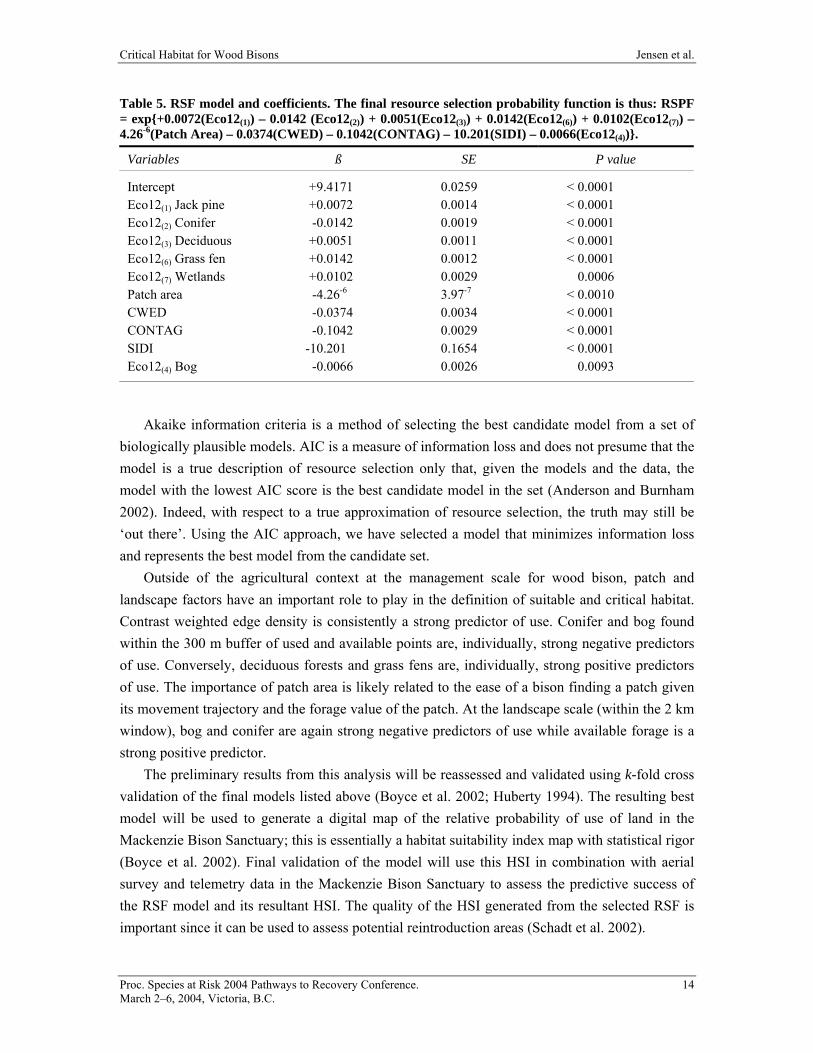
Resource selection function coefficients, standard errors, and P values from the model that best describe the data over the entire study area for all populations and all seasons are presented in Table 5. This model of habitat selection is a plausible description of suitable habitat for wood bison. Foraging requirements at the local and daily-movement scale are addressed by this model as are ecosites that have no value as forage and act as a barrier to movement, and consequently, result in energy loss in locomotion. Energy lost during travel within the landscape matrix is captured in the model by various friction or contrast indices including contrast weighted edge density, contagion, and Simpson’s diversity index.



Table 5. RSF model and coefficients. The final resource selection probability function is thus: RSPF = exp{+0.0072(Eco12(1)) – 0.0142 (Eco12(2)) + 0.0051(Eco12(3)) + 0.0142(Eco12(6)) + 0.0102(Eco12(7)) –4.26-6(Patch Area) – 0.0374(CWED) – 0.1042(CONTAG) – 10.201(SIDI) – 0.0066(Eco12(4))}.

Variables ß SE P value

Intercept +9.4171 0.0259 < 0.0001 Eco12(1) Jack pine +0.0072 0.0014 < 0.0001 Eco12(2) Conifer -0.0142 0.0019 < 0.0001 Eco12(3) Deciduous +0.0051 0.0011 < 0.0001 Eco12(6) Grass fen +0.0142 0.0012 < 0.0001 Eco12(7) Wetlands +0.0102 0.0029 0.0006 Patch area -4.26-6 3.97-7 < 0.0010 CWED -0.0374 0.0034 < 0.0001 CONTAG -0.1042 0.0029 < 0.0001 SIDI -10.201 0.1654 < 0.0001 Eco12(4) Bog -0.0066 0.0026 0.0093

Akaike information criteria is a method of selecting the best candidate model from a set of biologically plausible models. AIC is a measure of information loss and does not presume that the model is a true description of resource selection only that, given the models and the data, the model with the lowest AIC score is the best candidate model in the set (Anderson and Burnham 2002). Indeed, with respect to a true approximation of resource selection, the truth may still be ‘out there’. Using the AIC approach, we have selected a model that minimizes information loss and represents the best model from the candidate set.

Outside of the agricultural context at the management scale for wood bison, patch and landscape factors have an important role to play in the definition of suitable and critical habitat. Contrast weighted edge density is consistently a strong predictor of use. Conifer and bog found within the 300 m buffer of used and available points are, individually, strong negative predictors of use. Conversely, deciduous forests and grass fens are, individually, strong positive predictors of use. The importance of patch area is likely related to the ease of a bison finding a patch given its movement trajectory and the forage value of the patch. At the landscape scale (within the 2 km window), bog and conifer are again strong negative predictors of use while available forage is a strong positive predictor.

The preliminary results from this analysis will be reassessed and validated using k-fold cross validation of the final models listed above (Boyce et al. 2002; Huberty 1994). The resulting best model will be used to generate a digital map of the relative probability of use of land in the Mackenzie Bison Sanctuary; this is essentially a habitat suitability index map with statistical rigor (Boyce et al. 2002). Final validation of the model will use this HSI in combination with aerial survey and telemetry data in the Mackenzie Bison Sanctuary to assess the predictive success of the RSF model and its resultant HSI. The quality of the HSI generated from the selected RSF is important since it can be used to assess potential reintroduction areas (Schadt et al. 2002).



Conclusions

The results of this study suggest that for wood bison, the quality and type of vegetation surrounding forage habitat is important for determining both ease of locomotion and use for non-foraging activities such as ruminating, resting, and avoiding predation and harassment from biting flies. The conceptual model built on foraging theory, at least in the case of these free-roaming ruminants, is a reasonable basis upon which to build selection models for analysis within logistic regression. In this study, we measured immediate foraging and nonforaging needs by using a 300 m buffer around used points, and then daily life requirements within a larger landscape were measured. By using this technique, it appears that the multi-scale selection decisions made by foraging herds of wood bison have been captured. With the marginal value theorem and foraging theory itself as a conceptual base, we used landscape metrics as a tool for quantifying the probable energy loss resulting from locomotion in the landscape. Critical Habitat

Habitat is, by definition, suitable since it is “the resources and conditions present in an area to produce occupancy, including survival and reproduction of an organism” (Hall et al. 1997). Critical habitat as defined in SARA “means the habitat that is necessary for the survival or recovery of a listed wildlife species and that is identified as the species’ critical habitat in the recovery strategy or in an action plan for the species”: a term that is inextricably linked to recovery teams, recovery strategies, and SARA. In the case of wood bison, there may be many geographic locations that are considered habitat, and they can be objectively demarcated by using the RSF models and the resultant habitat suitability indices created in this study. The determination of critical habitat, since it relates to two explicit factors, population size (400 animals) and persistence over time, must be assessed using these RSF models in conjunction with population viability assessment (PVA). Habitat, as defined by the logistic regression model outlined above, can be spatially defined by incorporating the model coefficients and related data layers into a GIS. Existing used landscapes and potential reintroduction sites can then be assessed by quantifying forage habitat and mapping the relative probability of use of different spatial units. PVA can then be used, in the form of a metapopulation model, to assess the varying probabilities of persistence (under different land management or environmental scenarios) of the target herd surviving. In this case, the question would be, given a landscape and a resulting probability-of-use map, what is the probability of persistence of a herd of 400 animals in this landscape under the current land management regime? Designation, stewardship, and management follow a determination of high probability of persistence. We would designate a landscape as critical habitat if, using the suitable habitat map derived from the previous RSF model, we could obtain a PVA with a reasonably high score.



References Anderson, D.R., and K.P. Burnham. 2002. Avoiding pitfalls when using information-theoretic

methods. Journal of Wildlife Management 66:912–918. Beckingham, J.D., and J.H. Archibald. 1996. Field guide to the ecosites of Northern Alberta.

UBC Press, Vancouver, British Columbia. Bender, D.J., L. Tischendorf, and L. Fahrig. 2003. Using patch isolation metrics to predict animal

movement in binary landscapes. Landscape Ecology 18:17–39. Bergman, C.M., J.M. Fryxell, C.C. Gates, and D. Fortin. 2001. Ungulate foraging strategies:

energy maximizing or time minimizing? Journal of Animal Ecology 70:289–300. Boyce, M.S., and L.L. McDonald. 1999. Relating populations to habitats using resource selection

functions. TREE 14:268–272. Boyce, M.S., P.R. Vernier, S.E. Nielsen, and F.K.A. Schmiegelow. 2002. Evaluating resource

selection functions. Ecological Modeling 157:281–300. Carbyn, L.N., S.M. Oosenburg, and D.W. Anions. 1993. Wolves, bison and the dynamics related

to the Peace-Athabasca Delta in Canada’s Wood Buffalo National Park. Canadian Circumpolar Research Institute, Edmonton, Alberta.

Carbyn, L.N., N.J. Lunn, and K. Timoney. 1998. Trends in the distribution and abundance of

bison in Wood Buffalo National Park. Wildlife Society Bulletin 26:463–470. Committee on the Status of Endangered Wildlife in Canada (COSEWIC). 2001. Canadian

Species at Risk, November 2001. Committee on the Status of Endangered Wildlife in Canada Secretariat, Ottawa, Ontario.

Erickson, W.P., T.L. McDonald, and R. Skinner. 1998. Habitat selection using GIS: a case study.

Journal of Agricultural, Biological and Environmental Statistics 3:296–310. Fortin, D., J.M. Fryxell, and R. Pilote. 2002. The temporal scale of foraging decisions in bison.

Ecology 83:970–982. Fortin, D., J.M. Fryxell, L.O. O’Brodovich, and D. Frandsen. 2003. Foraging ecology of bison at

the landscape and plant community levels: the applicability of energy maximization principles. Oecologia 134:219–227.

Fuller, W.A. 2002. Canada and the “buffalo”, Bison bison: a tale of two herds. Canadian Field-

Naturalist 116:141–159. Gates, C.C., R.O. Stephenson, H.W. Reynolds, C.G. van Zyll de Jong, H. Schwantje, M. Hoefs, J.

Nishi, N. Cool, J. Chisholm, A. James, and B. Koonz. 2001. National Recovery Plan for the Wood Bison (Bison bison athabascae). National Recovery Plan No. 21. Canadian Wildlife Service, Ottawa, Ontario.

Hall, L.S., P.R. Krausman, and M.L. Morrison. 1997. The habitat concept and a plea for standard

terminology. Wildlife Society Bulletin 25:173–182.



Huberty, C.J. 1994. Applied discriminant analysis. John Wiley & Sons, New York, New York. Hudson, R.J., and S. Frank. 1987. Foraging ecology of bison in aspen boreal habitats. Journal of

Range Management 40:71–75. Jensen, O.C., and G.A. Sánchez-Azofeifa. In press. Satellite derived ecosystems classification:

image segmentation by ecological region for improved classification accuracy, a boreal case study. International Journal of Remote Sensing.

Johnson, D.H. 1980. Comparison of usage and availability measurements for evaluating resource

preference. Ecology 61:65–71. Joly, D.O., and F. Messier. 2001. Limiting effects of bovine brucellosis and tuberculosis on wood

bison within Wood Buffalo National Park. Final report, March 2001. University of Saskatchewan, Department of Biology, Saskatoon, Saskatchewan,

King, G., and L. Zeng. 2000. Logistic regression in rare events data. Annual Meetings of the

Society for Political Methodology. American Political Science Association, Washington, D.C.

Larter, N.C. 1988. Diet and habitat selection of an erupting wood bison population in the

Mackenzie Bison Sanctuary. MSc thesis. University of British Columbia, Vancouver, British Columbia.

Larter, N.C., and C.C. Gates. 1991. Diet and habitat selection of wood bison in relation to

seasonal changes in forage quantity and quality. Canadian Journal of Zoology 69:2677–2685.

McGarigal, K., S.A. Cushman, M.C. Neel, and E. Ene. 2002. FRAGSTATS: spatial pattern

analysis program for categorical maps. Computer software program produced by the authors at the University of Massachusetts, Amherst, Massachusetts. Available from www.umass.edu/landeco/research/fragstats/fragstats.html

Neu, C.W., C.R. Byers, and J.M. Peek. 1974. A technique for analysis of utilization-availability

data. Journal of Wildlife Management 38:541–545. Podani, J. 2001. SYN-TAX 2000: computer programs for data analysis in ecology and

systematics. Budapest, Hungary. Ponomarenko, S., and R. Alvo. 2001. Perspectives on developing a Canadian classification of

ecological communities. Natural Resources Canada, Hull, Quebec. Reynolds, H.W., R.M. Hansen, and D.G. Peden. 1978. Diets of the Slave River Lowlands bison

herd, Northwest Territories, Canada. Journal of Wildlife Management 42:581–590. Samuel, M.D., and K.P. Kenow 1992. Evaluating habitat selection with radio-telemetry

triangulation error. Journal of Wildlife Management 56:725–734.



Schadt, S., E. Revilla, T. Wiegand, F. Knauer, P. Kaczensky, U. Breitenmoser, L. Bufka, J. Cerveny, P. Koubek, T. Huber, C. Stanisa, and L. Trepl. 2002. Assessing the suitability of central European landscapes for the reintroduction of Eurasian lynx. Journal of Applied Ecology 39:189–203.

Stephens, D.W., and J.R. Krebs. 1986. Foraging theory. Princeton University Press, Princeton,

New Jersey. Taylor, M.K., S. Akeeagok, D. Andiashek, W. Barbour, E.W. Born, W. Calvert, H.D. Cluff, S.

Ferguson, J. Laake, A. Rosing-Asvid, I. Stirling, and F. Messier. 2001. Delineating Canadian and Greenland polar bear (Ursus maritimus) populations by cluster analysis of movements. Canadian Journal of Zoology 79:690–709.

Wells, J.V., and M.E. Richmond. 1995. Populations, metapopulations, and species populations:

what are they and who should care? Wildlife Society Bulletin 23:458–462.


Assessing Suitable and Critical Habitat for Wood Bison (Bison bison athabascae) Using Geographic...

Documents

Transcript of Assessing Suitable and Critical Habitat for Wood Bison (Bison bison athabascae) Using Geographic...