
Ascent Documentation - Read the Docs
401
Ascent Documentation Release 0.8.0 LLNS Aug 31, 2022
-
Upload
khangminh22 -
Category
Documents
-
view
2 -
download
0
Transcript of Ascent Documentation - Read the Docs

Ascent DocumentationRelease 0.8.0
LLNS
Aug 31, 2022


Contents
1 Learn how to use Ascent with Docker + Jupyter 3
2 Introduction 5
3 Ascent Project Resources 7
4 Ascent Documentation 9
5 Indices and tables 395
Index 397
i

ii

Ascent Documentation, Release 0.8.0
Ascent is a many-core capable flyweight in situ visualization and analysis infrastructure for multi-physics HPC simu-lations.
Contents 1

Ascent Documentation, Release 0.8.0
2 Contents

CHAPTER 1
Learn how to use Ascent with Docker + Jupyter
If you have Docker, an easy way to learn about Ascent is to run our prebuilt Docker container:
docker run -p 8888:8888 -t -i alpinedav/ascent-jupyter
Then open http://localhost:8888 in your browser to connect to the Jupyter Server in the container. The password forthe Jupyter server is: learn. From here, you can run Ascent’s Python Tutorial Notebook examples. For more detailssee our Ascent Tutorial.
3

Ascent Documentation, Release 0.8.0
4 Chapter 1. Learn how to use Ascent with Docker + Jupyter

CHAPTER 2
Introduction
Ascent is an easy-to-use flyweight in situ visualization and analysis library for HPC simulations:
• Supports: Making Pictures, Transforming Data, and Capturing Data for use outside of Ascent
• Young effort, yet already includes most common visualization operations
• Provides a simple infrastructure to integrate custom analysis
• Provides C++, C, Python, and Fortran APIs
Ascent’s flyweight design targets next-generation HPC platforms:
• Provides efficient distributed-memory (MPI) and many-core (CUDA or OpenMP) execution
• Demonstrated scaling: In situ filtering and ray tracing across 16,384 GPUs on LLNL’s Sierra Cluster
• Has lower memory requirements than current tools
• Requires less dependencies than current tools (ex: no OpenGL)
Ascent focuses on ease of use and reducing integration burden for simulation code teams:
• Actions are passed to Ascent via YAML files
• Replay capability helps prototype and test actions
• It does not require GUI or system-graphics libraries
• It includes integration examples that demonstrate how to use Ascent inside existing HPC-simulation proxyapplications
2.1 The Great Amalgamation
The VTK-h, Devil Ray, and AP Compositor projects are now developed in Ascent’s source instead of separate repos.These external repos for these projects are archived. This reorg simplifies the development and support of these tightlycoupled capabilities. Ascent 0.9.0 will be the first release using these internal versions.
5

Ascent Documentation, Release 0.8.0
2.2 Getting Started
To get started building and using Ascent, see the Quick Start Guide and the Ascent Tutorial. For more details aboutbuilding Ascent see the Building documentation.
6 Chapter 2. Introduction

CHAPTER 3
Ascent Project Resources
Website and Online Documentation
http://www.ascent-dav.org
Github Source Repo
http://github.com/alpine-dav/ascent
Issue Tracker
http://github.com/llnl/ascent/issues
Help Email
Contributors
https://github.com/Alpine-DAV/ascent/graphs/contributors
7

Ascent Documentation, Release 0.8.0
8 Chapter 3. Ascent Project Resources

CHAPTER 4
Ascent Documentation
4.1 Quick Start
4.1.1 Running Ascent via Docker
The easiest way to try out Ascent is via our Docker container. If you have Docker installed you can obtain a Dockerimage with a ready-to-use ascent install from Docker Hub. This image also includes a Jupyter install to supportrunning Ascent’s tutorial notebooks.
To start the Jupyter server and run the tutorial notebooks, run:
docker run -p 8888:8888 -t -i alpinedav/ascent-jupyter
(The -p is used to forward ports between the container and your host machine, we use these ports to allow web serverson the container to serve data to the host.)
This container automatically launches a Jupyter Notebook server on port 8888. Assuming you forwarded port 8888from the Docker container to your host machine, you should be able to connect to the notebook server using http://localhost:8888. The password for the notebook server is: learn
4.1.2 Installing Ascent and Third Party Dependencies
The quickest path to install Ascent and its dependencies is via uberenv:
git clone --recursive https://github.com/alpine-dav/ascent.gitcd ascentpython scripts/uberenv/uberenv.py --install --prefix="build"
After this completes, build/ascent-install will contain an Ascent install.
We also provide spack settings for several well known HPC clusters, here is an example of how to use our settings forOLCF’s Summit System:
9

Ascent Documentation, Release 0.8.0
python scripts/uberenv/uberenv.py --install --prefix="build" --spack-config-dir=→˓"scripts/uberenv_configs/spack_configs/configs/olcf/summit_gcc_9.3.0_cuda_11.0.3/"
For more details about building and installing Ascent see Building Ascent. This page provides detailed info aboutAscent’s CMake options, uberenv and Spack support. We also provide info about building for known HPC clustersusing uberenv and a Docker example that leverages Spack.
4.1.3 Public Installs of Ascent
We also provide public installs of Ascent for the default compilers at a few DOE HPC centers.
Summary table of public ascent installs:
Site System CompilerRuntime Modules Install PathOLCF Summit gcc
9.3.0CUDA11.0.3
gcc/9.3.0cuda/11.0.3
/sw/summit/ums/ums010/ascent/current/summit/cuda/gnu/ascent-install/
OLCF Summit gcc9.3.0
OpenMP gcc/9.3.0 /sw/summit/ums/ums010/ascent/current/summit/openmp/gnu/ascent-install/
NERSC Permutter gcc9.3.0
CUDA11.4.0
PrgEnv-gnucpe-cuda/21.12cudatoolkit/21.9_11.4
/global/cfs/cdirs/alpine/software/ascent/current/perlmutter/cuda/gnu/ascent-install/
LLNLLC
CZ TOSS 3(Pascal)
gcc4.9.3
OpenMP (none) /usr/gapps/conduit/software/ascent/current/toss_3_x86_64_ib/openmp/gnu/ascent-install
Here is a link to the scripts we use to build public Ascent installs.
See Using Public Installs of Ascent for more details on using these installs.
4.1.4 Using Ascent in Your Project
The install includes examples that demonstrate how to use Ascent in a CMake-based build system and via a Makefile.
CMake-based build system example (see: examples/ascent/using-with-cmake):
################################################################################# Example that shows how to use an installed instance of Ascent in another# CMake-based build system.## To build:# mkdir build# cd build# cmake -DAscent_DIR={ascent install path} ../# make# ./ascent_render_example## In order to run directly in a sub directory below using-with-cmake in an ascent→˓install,
(continues on next page)
10 Chapter 4. Ascent Documentation

Ascent Documentation, Release 0.8.0
(continued from previous page)
# set Ascent_DIR to ../../..## mkdir build# cd build# cmake .. -DAscent_DIR=../../..# make# ./ascent_render_example################################################################################
cmake_minimum_required(VERSION 3.9)
project(using_with_cmake)
## Use CMake's find_package to import ascent's targets## PATHS is just a hint if someone runs this example from the Ascent install# tree without setting up an environment hint to find Ascentfind_package(Ascent REQUIRED
NO_DEFAULT_PATHPATHS ${CMAKE_SOURCE_DIR}/../../../)
# create our exampleadd_executable(ascent_render_example ascent_render_example.cpp)
# link to ascenttarget_link_libraries(ascent_render_example ascent::ascent)
# if cuda is in the mix:# we need to make sure CUDA_RESOLVE_DEVICE_SYMBOLS is on for our target# (it propgates some way magically in 3.14, but not in 3.21)if(CMAKE_CUDA_COMPILER)
set_property(TARGET ascent_render_example PROPERTY CUDA_RESOLVE_DEVICE_SYMBOLS ON)endif()
CMake-based build system example with MPI (see: examples/ascent/using-with-cmake-mpi):
# Example that shows how to use an installed instance of Ascent in another# CMake-based build system.## To build:# cmake -DAscent_DIR={ascent install path} -B build -S .# cd build# make# mpiexec -n 2 ./ascent_mpi_render_example## In order to run directly in a sub directory below using-with-cmake-mpi in an ascent→˓install,# set Ascent_DIR to ../../..## cmake -DAscent_DIR={ascent install path} -B build -S .# cd build# make# mpiexec -n 2 ./ascent_mpi_render_example################################################################################
(continues on next page)
4.1. Quick Start 11

Ascent Documentation, Release 0.8.0
(continued from previous page)
cmake_minimum_required(VERSION 3.9)
project(using_with_cmake)
## Use CMake's find_package to import ascent's targets## PATHS is just a hint if someone runs this example from the Ascent install# tree without setting up an environment hint to find Ascentfind_package(Ascent REQUIRED
NO_DEFAULT_PATHPATHS ${CMAKE_SOURCE_DIR}/../../../)
# create our exampleadd_executable(ascent_mpi_render_example ascent_mpi_render_example.cpp)
# link to ascenttarget_link_libraries(ascent_mpi_render_example ascent::ascent_mpi)
# if cuda is in the mix:# we need to make sure CUDA_RESOLVE_DEVICE_SYMBOLS is on for our target# (it propgates some way magically in 3.14, but not in 3.21)if(CMAKE_CUDA_COMPILER)
set_property(TARGET ascent_mpi_render_example PROPERTY CUDA_RESOLVE_DEVICE_SYMBOLS→˓ON)endif()
Makefile-based build system example (see: examples/ascent/using-with-make):
################################################################################# Example that shows how to use an installed instance of Ascent in Makefile# based build system.## To build:# env ASCENT_DIR={ascent install path} make# ./ascent_render_example## From within an ascent install:# make# ./ascent_render_example## Which corresponds to:## make ASCENT_DIR=../../../# ./ascent_render_example################################################################################
ASCENT_DIR ?= ../../..
# See $(ASCENT_DIR)/share/ascent/ascent_config.mk for detailed linking infoinclude $(ASCENT_DIR)/share/ascent/ascent_config.mk
(continues on next page)
12 Chapter 4. Ascent Documentation

Ascent Documentation, Release 0.8.0
(continued from previous page)
# make sure to enable c++11 support (conduit's interface now requires it)CXX_FLAGS = -std=c++11INC_FLAGS = $(ASCENT_INCLUDE_FLAGS)LNK_FLAGS = $(ASCENT_LINK_RPATH) $(ASCENT_LIB_FLAGS)
main:$(CXX) $(CXX_FLAGS) $(INC_FLAGS) ascent_render_example.cpp $(LNK_FLAGS) -o
→˓ascent_render_example
clean:rm -f ascent_render_example
Makefile-based build system example with MPI (see: examples/ascent/using-with-make-mpi):
################################################################################# Example that shows how to use an installed instance of Ascent in Makefile# based build system.## To build:# env ASCENT_DIR={ascent install path} make# ./ascent_render_example## From within an ascent install:# make# mpiexec -n 2 ./ascent_mpi_render_example## Which corresponds to:## make ASCENT_DIR=../../../# mpiexec -n 2 ./ascent_mpi_render_example################################################################################
ASCENT_DIR ?= ../../..
# See $(ASCENT_DIR)/share/ascent/ascent_config.mk for detailed linking infoinclude $(ASCENT_DIR)/share/ascent/ascent_config.mk
# make sure to enable c++11 support (conduit's interface now requires it)CXX_FLAGS = -std=c++11INC_FLAGS = $(ASCENT_INCLUDE_FLAGS)LNK_FLAGS = $(ASCENT_LINK_RPATH) $(ASCENT_MPI_LIB_FLAGS)
main:$(CXX) $(CXX_FLAGS) $(INC_FLAGS) ascent_mpi_render_example.cpp $(LNK_FLAGS) -
→˓o ascent_mpi_render_example
clean:rm -f ascent_mpi_render_example
4.1. Quick Start 13

Ascent Documentation, Release 0.8.0
4.2 Tutorial Overview
Ascent Tutorial Intro Slides [pdf]
This tutorial introduces how to use Ascent, including basics about:
• Formatting mesh data for Ascent
• Using Conduit and Ascent’s Conduit-based API
• Using and combining Ascent’s core building blocks: Scenes, Pipelines, Extracts, Queries, and Triggers
• Using Ascent with the Cloverleaf3D example integration
Ascent installs include standalone C++, Python, and Python-based Jupyter notebook examples for this tutorial.You can find the tutorial source code and notebooks in your Ascent install directory under examples/ascent/tutorial/ascent_intro/ and the Cloverleaf3D demo files under examples/ascent/tutorial/cloverleaf_demos/.
Scheduled Tutorials:
• Introduction to Ascent, a Flyweight In Situ Visualization and Analysis for HPC Simulations @ LLNL’s RA-DIUSS AWS Tutorial Series 2022 - August 2022, Virtual
Past Tutorials:
• In Situ Analysis and Visualization with ParaView Catalyst and Ascent @ ISC 2022 - May 2022, Hamburg,Germany
• ECP 2022 Annual Meeting - May 2022, Virtual
• In Situ Analysis and Visualization with SENSEI and Ascent @ SC21 - Nov 2021, Virtual
• ECP 2021 Annual Meeting - April 2021, Virtual
• In Situ Scientific Analysis and Visualization using ALPINE Ascent @ ECP Training Event - Dec 2020,Virtual
• In Situ Analysis and Visualization with SENSEI and Ascent @ SC20 - Nov 2020, Virtual
• ECP 2020 Annual Meeting - Feb 2020, Houston, TX, USA
• In Situ Analysis and Visualization with SENSEI and Ascent @ SC19 - Nov 2019, Denver, CO, USA
• ECP 2019 Annual Meeting - Jan 2019, Houston, TX, USA
• ECP 2018 Annual Meeting - Feb 2018, Knoxville, TX, USA
4.3 Tutorial Setup
The tutorial examples are installed with Ascent to the subdirectory examples/ascent/tutorial/. Below areseveral options for using pre-built Ascent installs and links to info about building Ascent. If you have access to Docker,the easiest way to test the waters is via the alpinedav/ascent Docker image.
4.3.1 Tutorial Cloud Option
For in person tutorials (at Supercomputing, the ECP Annual Meeting, etc), we provide HTTP access to several in-stances of our Ascent Docker image running the jupyter notebook server. We hand out IP addresses and login info toattendees during these events.
14 Chapter 4. Ascent Documentation

Ascent Documentation, Release 0.8.0
4.3.2 Using Docker
If you have Docker installed you can obtain a Docker image with a ready-to-use ascent install from Docker Hub. Thisimage also includes a Jupyter install to support running Ascent’s tutorial notebooks.
To directly start the Jupyter Notebook server and run the tutorial notebooks, run:
docker run -p 8888:8888 -t -i alpinedav/ascent-jupyter
(The -p is used to forward ports between the container and your host machine, we use these ports to allow web serverson the container to serve data to the host.)
This image automatically launches a Jupyter Notebook server on port 8888. Assuming you forwarded port 8888 fromthe Docker container to your host machine, you should be able to connect to the notebook server using http://localhost:8888. The current password for the notebook server is: learn
To start the base image and explore the install and tutorial examples with bash, run:
docker run -p 8888:8888 -t -i alpinedav/ascent
You will now be at a bash prompt in you container.
To add the proper paths to Python and MPI to your environment, run:
source ascent_docker_setup_env.sh
The ascent source code is at /ascent/src/, and the install is at /ascent/install/. The tutorial exam-ples are at /ascent/install/examples/ascent/tutorial/ and the tutorial notebooks are at /ascent/install/examples/ascent/tutorial/ascent_intro/notebooks/.
You can also launch the a Jupyter Notebook server from this image using the following:
./ascent_docker_run_jupyter.sh
The url (http://localhost:8888) and password (learn) are the same as above.
4.3.3 Using Public Installs of Ascent
This section provides info about public installs we provide on several HPC machines.
Additionally, here is a link to the scripts used to build our public installs .
OLCF Summit Installs
• Build Details: gcc 9.3.0 with OpenMP and MPI support
• Modules: gcc/9.3.0
• Location: /sw/summit/ums/ums010/ascent/current/summit/openmp/gnu/ascent-install/
You can copy the tutorial examples from this install and use them as follows:
#!/bin/bash## source helper script that loads modules, sets python paths, and ASCENT_DIR env var#source /sw/summit/ums/ums010/ascent/current/summit/ascent_summit_setup_env_gcc_openmp.→˓sh (continues on next page)
4.3. Tutorial Setup 15

Ascent Documentation, Release 0.8.0
(continued from previous page)
export LD_LIBRARY_PATH=$LD_LIBRARY_PATH:/sw/summit/ums/ums010/ascent/current/summit/→˓openmp/gnu/python-install/lib/
## make your own dir to hold the tutorial examples#mkdir ascent_tutorialcd ascent_tutorial
## copy the examples from the public install#cp -r /sw/summit/ums/ums010/ascent/current/summit/openmp/gnu/ascent-install/examples/→˓ascent/tutorial/* .
## build cpp examples and run the first one#cd ascent_intro/cppmakeenv OMP_NUM_THREADS=1 ./ascent_first_light_example
## run a python example#cd ..cd pythonenv OMP_NUM_THREADS=1 python ascent_first_light_example.py
• Build Details: gcc 9.3.0 with CUDA 11.0.3 and MPI support
• Modules: gcc/9.3.0 cuda/11.0.3
• Location: /sw/summit/ums/ums010/ascent/current/summit/cuda/gnu/ascent-install/
You can copy the tutorial examples from this install and use them as follows:
#!/bin/bash## source helper script that loads modules, sets python paths, and ASCENT_DIR env var#source /sw/summit/ums/ums010/ascent/current/summit/ascent_summit_setup_env_gcc_cuda.sh
## make your own dir to hold the tutorial examples#mkdir ascent_tutorialcd ascent_tutorial
## copy the examples from the public install#cp -r /sw/summit/ums/ums010/ascent/current/summit/cuda/gnu/ascent-install/examples/→˓ascent/tutorial/* .
## build cpp examples and run the first one
(continues on next page)
16 Chapter 4. Ascent Documentation

Ascent Documentation, Release 0.8.0
(continued from previous page)
#cd ascent_intro/cppmake./ascent_first_light_example
NERSC Perlmuter Install
• Build Details: gcc 10.3.0 with CUDA 11.4.0 and MPI support
• Modules: PrgEnv-gnu cpe-cuda/21.12 cudatoolkit/21.9_11.4
• Location: /global/cfs/cdirs/alpine/software/ascent/current/perlmutter/cuda/gnu/ascent-install/
You can copy the tutorial examples from this install and use them as follows:
#!/bin/bash## source helper script that loads modules, sets python paths, and ASCENT_DIR env var#source /global/cfs/cdirs/alpine/software/ascent/current/cori/ascent_permutter_setup_→˓env_gcc_cuda.sh
## make your own dir to hold the tutorial examples#mkdir ascent_tutorialcd ascent_tutorial
## copy the examples from the public install#cp -r /global/cfs/cdirs/alpine/software/ascent/current/perlmutter/cuda/gnu/ascent-→˓install/examples/ascent/tutorial/* .
## build cpp examples and run the first one#cd ascent_intro/cppmake./ascent_first_light_example
LLNL CZ TOSS 3 Install
• Build Details: gcc 4.9.3 with OpenMP and MPI support
• Modules: (none)
• Location: /usr/gapps/conduit/software/ascent/current/toss_3_x86_64_ib/openmp/gnu/ascent-install/
You can copy the tutorial examples from this install and use them as follows:
#!/bin/bash## source helper script that loads modules, sets python paths, and ASCENT_DIR env var
(continues on next page)
4.3. Tutorial Setup 17

Ascent Documentation, Release 0.8.0
(continued from previous page)
#source /usr/gapps/conduit/software/ascent/current/toss_3_x86_64_ib/ascent_toss_3_x86_→˓64_ib_setup_env_gcc_openmp.sh
## make your own dir to hold the tutorial examples#mkdir ascent_tutorialcd ascent_tutorial
## copy the examples from the public install#cp -r /usr/gapps/conduit/software/ascent/current/toss_3_x86_64_ib/openmp/gnu/ascent-→˓install/examples/ascent/tutorial/* .
## build cpp examples and run the first one#cd ascent_intro/cppmakeenv OMP_NUM_THREADS=1 ./ascent_first_light_example
## run a python example#cd ..cd pythonenv OMP_NUM_THREADS=1 python ascent_first_light_example.py
Register Ascent’s Python as a Jupyter Kernel
Warning: This works the LLNL LC TOSS3 CZ OpenMP install, we are working on recipes for other HPCcenters.
You can register Ascent’s Python as a custom Jupyter kernel with Jupyter Hub.
LLNL CZ TOSS 3 Jupyter Kernel Register Example:
#!/bin/bash## source helper script that loads modules, sets python paths, and ASCENT_DIR env var#source /usr/gapps/conduit/software/ascent/current/toss_3_x86_64_ib/ascent_toss_3_x86_→˓64_ib_setup_env_gcc_openmp.sh
## Register Ascent's Python with Jupyter Hub#python -m ipykernel install --user --name ascent_kernel --display-name "Ascent Kernel"
After you register you will see an option to launch an Ascent kernel in Jupyter Hub:
18 Chapter 4. Ascent Documentation

Ascent Documentation, Release 0.8.0
With this kernel you can access Ascent’s Python modules or run the tutorial notebooks:
If you want to remove the registered kernel, you can use:
# show list of registered kernelsjupyter kernelspec list# remove our Ascent custom kerneljupyter kernelspec uninstall ascent_kernel
4.3.4 Build and Install
To build and install Ascent yourself see Quick Start.
4.4 Introduction to Ascent
4.4.1 First Light
4.4. Introduction to Ascent 19

Ascent Documentation, Release 0.8.0
Render a sample dataset using Ascent
To start, we run a basic “First Light” example to generate an image. This example renders the an example datasetusing ray casting to create a pseudocolor plot. The dataset is one of the built-in Conduit Mesh Blueprint examples, inthis case an unstructured mesh composed of hexagons.
C++ Source
#include <iostream>
#include "ascent.hpp"#include "conduit_blueprint.hpp"
using namespace ascent;using namespace conduit;
int main(int argc, char **argv){
// echo info about how ascent was configuredstd::cout << ascent::about() << std::endl;
// create conduit node with an example mesh using// conduit blueprint's braid function// ref: https://llnl-conduit.readthedocs.io/en/latest/blueprint_mesh.html#braid
// things to explore:// changing the mesh resolution
Node mesh;conduit::blueprint::mesh::examples::braid("hexs",
50,50,50,mesh);
// create an Ascent instanceAscent a;
// open ascenta.open();
// publish mesh data to ascenta.publish(mesh);
//// Ascent's interface accepts "actions"// that to tell Ascent what to execute//Node actions;Node &add_act = actions.append();add_act["action"] = "add_scenes";
// Create an action that tells Ascent to:// add a scene (s1) with one plot (p1)// that will render a pseudocolor of// the mesh field `braid`Node & scenes = add_act["scenes"];
(continues on next page)
20 Chapter 4. Ascent Documentation

Ascent Documentation, Release 0.8.0
(continued from previous page)
// things to explore:// changing plot type (mesh)// changing field name (for this dataset: radial)scenes["s1/plots/p1/type"] = "pseudocolor";scenes["s1/plots/p1/field"] = "braid";// set the output file name (ascent will add ".png")scenes["s1/image_name"] = "out_first_light_render_3d";
// view our full actions treestd::cout << actions.to_yaml() << std::endl;
// execute the actionsa.execute(actions);
// close ascenta.close();
}
Python Source
import conduitimport conduit.blueprintimport ascent
# print details about ascentprint(ascent.about().to_yaml())
# create conduit node with an example mesh using conduit blueprint's braid function# ref: https://llnl-conduit.readthedocs.io/en/latest/blueprint_mesh.html#braid
# things to explore:# changing the mesh resolution
mesh = conduit.Node()conduit.blueprint.mesh.examples.braid("hexs",
50,50,50,mesh)
# create an Ascent instancea = ascent.Ascent()
# set options to allow errors propagate to pythonascent_opts = conduit.Node()ascent_opts["exceptions"] = "forward"
## open ascent#a.open(ascent_opts)
## publish mesh data to ascent#a.publish(mesh)
(continues on next page)
4.4. Introduction to Ascent 21

Ascent Documentation, Release 0.8.0
(continued from previous page)
## Ascent's interface accepts "actions"# that to tell Ascent what to execute#actions = conduit.Node()
# Create an action that tells Ascent to:# add a scene (s1) with one plot (p1)# that will render a pseudocolor of# the mesh field `braid`add_act = actions.append()add_act["action"] = "add_scenes"
# declare a scene (s1) and pseudocolor plot (p1)scenes = add_act["scenes"]
# things to explore:# changing plot type (mesh)# changing field name (for this dataset: radial)scenes["s1/plots/p1/type"] = "pseudocolor"scenes["s1/plots/p1/field"] = "braid"
# set the output file name (ascent will add ".png")scenes["s1/image_name"] = "out_first_light_render_3d"
# view our full actions treeprint(actions.to_yaml())
# execute the actionsa.execute(actions)
# close ascenta.close()
4.4.2 Conduit Basics
Ascent’s API is based on Conduit. Both mesh data and action descriptions are passed to Ascent as Conduit trees. TheConduit C++ and Python interfaces are very similar, with the C++ interface heavily influenced by the ease of use ofPython. These examples provide basic knowledge about creating Conduit Nodes to use with Ascent. You can also findmore introductory Conduit examples in Conduit’s Tutorial Docs .
Creating key-value entries
C++ Source
#include <iostream>#include <vector>#include "conduit.hpp"
using namespace conduit;
int main(){
//(continues on next page)
22 Chapter 4. Ascent Documentation

Ascent Documentation, Release 0.8.0
Fig. 4.1: First Light Example Result
4.4. Introduction to Ascent 23

Ascent Documentation, Release 0.8.0
(continued from previous page)
// The core of Conduit's data model is `Node` object that// holds a dynamic hierarchical key value tree//// Here is a simple example that creates// a key value pair in a Conduit Node://Node n;n["key"] = "value";std::cout << n.to_yaml() << std::endl;
}
Output
key: "value"
Python Source
import conduitimport numpy as np
## The core of Conduit's data model is `Node` object that# holds a dynamic hierarchical key value tree## Here is a simple example that creates# a key value pair in a Conduit Node:#n = conduit.Node()n["key"] = "value";print(n.to_yaml())
Output
key: "value"
Creating a path hierarchy
C++ Source
#include <iostream>#include <vector>#include "conduit.hpp"
using namespace conduit;
int main(){
//// Using hierarchical paths imposes a tree structure//Node n;n["dir1/dir2/val1"] = 100.5;std::cout << n.to_yaml() << std::endl;
}
Output
24 Chapter 4. Ascent Documentation

Ascent Documentation, Release 0.8.0
dir1:dir2:val1: 100.5
Python Source
import conduitimport numpy as np
## Using hierarchical paths imposes a tree structure#n = conduit.Node()n["dir1/dir2/val1"] = 100.5;print(n.to_yaml())
Output
dir1:dir2:val1: 100.5
Setting array data
C++ Source
#include <iostream>#include <vector>#include "conduit.hpp"
using namespace conduit;
int main(){
//// Conduit's Node trees hold strings or bitwidth style numeric array leaves//// In C++: you can pass raw pointers to numeric arrays or// std::vectors with numeric values//// In python: numpy ndarrays are used for arrays//
Node n;int *A = new int[10];A[0] = 0;A[1] = 1;for (int i = 2 ; i < 10 ; i++)
A[i] = A[i-2]+A[i-1];n["fib"].set(A, 10);
std::cout << n.to_yaml() << std::endl;
delete [] A;}
Output
4.4. Introduction to Ascent 25

Ascent Documentation, Release 0.8.0
fib: [0, 1, 1, 2, 3, 5, 8, 13, 21, 34]
Python Source
import conduitimport numpy as np
## Conduit's Node trees hold strings or bitwidth style numeric array leaves## In C++: you can pass raw pointers to numeric arrays or# std::vectors with numeric values## In python: numpy ndarrays are used for arrays#n = conduit.Node()a = np.zeros(10, dtype=np.int32)
a[0] = 0a[1] = 1for i in range(2,10):
a[i] = a[i-2] + a[i-1]
n["fib"].set(a);print(n.to_yaml());
Output
fib: [0, 1, 1, 2, 3, 5, 8, 13, 21, 34]
Zero-copy vs deep copy of array data
C++ Source
#include <iostream>#include <vector>#include "conduit.hpp"
using namespace conduit;using std::vector;
int main(){
//// Conduit supports zero copy, allowing a Conduit Node to describe and// point to externally allocated data.//// set_external() is method used to zero copy data into a Node//
Node n;vector<int> A1(10);A1[0] = 0;A1[1] = 1;for (int i = 2 ; i < 10 ; i++)
A1[i] = A1[i-2]+A1[i-1];
(continues on next page)
26 Chapter 4. Ascent Documentation

Ascent Documentation, Release 0.8.0
(continued from previous page)
n["fib_deep_copy"].set(A1);
// create another array to demo difference// between set and set_externalvector<int> A2(10);
A2[0] = 0;A2[1] = 1;for (int i = 2 ; i < 10 ; i++){
A2[i] = A2[i-2]+A2[i-1];}
n["fib_shallow_copy"].set_external(A2);A1[9] = -1;A2[9] = -1;
std::cout << n.to_yaml() << std::endl;}
Output
fib_deep_copy: [0, 1, 1, 2, 3, 5, 8, 13, 21, 34]fib_shallow_copy: [0, 1, 1, 2, 3, 5, 8, 13, 21, -1]
Python Source
import conduitimport numpy as np
## Conduit supports zero copy, allowing a Conduit Node to describe and# point to externally allocated data.## set_external() is method used to zero copy data into a Node#n = conduit.Node()a1 = np.zeros(10, dtype=np.int32)
a1[0] = 0a1[1] = 1
for i in range(2,10):a1[i] = a1[i-2] + a1[i-1]
# create another array to demo difference# between set and set_externala2 = np.zeros(10, dtype=np.int32)
a2[0] = 0a2[1] = 1
for i in range(2,10):a2[i] = a2[i-2] + a2[i-1]
n["fib_deep_copy"].set(a1);(continues on next page)
4.4. Introduction to Ascent 27

Ascent Documentation, Release 0.8.0
(continued from previous page)
n["fib_shallow_copy"].set_external(a2);
a1[-1] = -1a2[-1] = -1
print(n.to_yaml())
Output
fib_deep_copy: [0, 1, 1, 2, 3, 5, 8, 13, 21, 34]fib_shallow_copy: [0, 1, 1, 2, 3, 5, 8, 13, 21, -1]
4.4.3 Conduit Blueprint Mesh Examples
Simulation mesh data is passed to Ascent using a shared set of conventions called the Mesh Blueprint.
Simply described, these conventions outline a structure to follow to create Conduit trees that can represent a wide rangeof simulation mesh types (uniform grids, unstructured meshes, etc). Conduit’s dynamic tree and zero-copy supportmake it easy to adapt existing data to conform to the Mesh Blueprint for use in tools like Ascent.
These examples outline how to create Conduit Nodes that describe simple single domain meshes and review someof Conduits built-in mesh examples. More Mesh Blueprint examples are also detailed in Conduit’s Mesh BlueprintExamples Docs .
Creating a uniform grid with a single field
C++ Source
#include <iostream>#include "ascent.hpp"#include "conduit_blueprint.hpp"
using namespace ascent;using namespace conduit;
int main(int argc, char **argv){
//// Create a 3D mesh defined on a uniform grid of points// with a single vertex associated field named `alternating`//Node mesh;
int numPerDim = 9;// create the coordinate setmesh["coordsets/coords/type"] = "uniform";mesh["coordsets/coords/dims/i"] = numPerDim;mesh["coordsets/coords/dims/j"] = numPerDim;mesh["coordsets/coords/dims/k"] = numPerDim;
// add origin and spacing to the coordset (optional)mesh["coordsets/coords/origin/x"] = -10.0;mesh["coordsets/coords/origin/y"] = -10.0;mesh["coordsets/coords/origin/z"] = -10.0;
(continues on next page)
28 Chapter 4. Ascent Documentation

Ascent Documentation, Release 0.8.0
(continued from previous page)
double distancePerStep = 20.0/(numPerDim-1);mesh["coordsets/coords/spacing/dx"] = distancePerStep;mesh["coordsets/coords/spacing/dy"] = distancePerStep;mesh["coordsets/coords/spacing/dz"] = distancePerStep;
// add the topology// this case is simple b/c it's implicitly derived from the coordinate setmesh["topologies/topo/type"] = "uniform";// reference the coordinate set by namemesh["topologies/topo/coordset"] = "coords";
int numVertices = numPerDim*numPerDim*numPerDim; // 3Dfloat *vals = new float[numVertices];for (int i = 0 ; i < numVertices ; i++)
vals[i] = ( (i%2)==0 ? 0.0 : 1.0);
// create a vertex associated field named alternatingmesh["fields/alternating/association"] = "vertex";mesh["fields/alternating/topology"] = "topo";mesh["fields/alternating/values"].set_external(vals, numVertices);
// print the mesh we createdstd::cout << mesh.to_yaml() << std::endl;
// make sure the mesh we created conforms to the blueprint
Node verify_info;if(!blueprint::mesh::verify(mesh, verify_info)){
std::cout << "Mesh Verify failed!" << std::endl;std::cout << verify_info.to_yaml() << std::endl;
}else{
std::cout << "Mesh verify success!" << std::endl;}
// now lets look at the mesh with AscentAscent a;
// open ascenta.open();
// publish mesh to ascenta.publish(mesh);
// setup actionsNode actions;Node &add_act = actions.append();add_act["action"] = "add_scenes";
// declare a scene (s1) with one plot (p1)// to render the datasetNode &scenes = add_act["scenes"];scenes["s1/plots/p1/type"] = "pseudocolor";scenes["s1/plots/p1/field"] = "alternating";// Set the output file name (ascent will add ".png")
(continues on next page)
4.4. Introduction to Ascent 29

Ascent Documentation, Release 0.8.0
(continued from previous page)
scenes["s1/image_prefix"] = "out_ascent_render_uniform";
// print our full actions treestd::cout << actions.to_yaml() << std::endl;
// execute the actionsa.execute(actions);
// close ascenta.close();
}
Python Source
import conduitimport conduit.blueprintimport ascentimport numpy as np
## Create a 3D mesh defined on a uniform grid of points# with a single vertex associated field named `alternating`#
mesh = conduit.Node()
# create the coordinate setnum_per_dim = 9mesh["coordsets/coords/type"] = "uniform";mesh["coordsets/coords/dims/i"] = num_per_dimmesh["coordsets/coords/dims/j"] = num_per_dimmesh["coordsets/coords/dims/k"] = num_per_dim
# add origin and spacing to the coordset (optional)mesh["coordsets/coords/origin/x"] = -10.0mesh["coordsets/coords/origin/y"] = -10.0mesh["coordsets/coords/origin/z"] = -10.0
distance_per_step = 20.0/(num_per_dim-1)
mesh["coordsets/coords/spacing/dx"] = distance_per_stepmesh["coordsets/coords/spacing/dy"] = distance_per_stepmesh["coordsets/coords/spacing/dz"] = distance_per_step
# add the topology# this case is simple b/c it's implicitly derived from the coordinate setmesh["topologies/topo/type"] = "uniform";# reference the coordinate set by namemesh["topologies/topo/coordset"] = "coords";
# create a vertex associated field named alternatingnum_vertices = num_per_dim * num_per_dim * num_per_dimvals = np.zeros(num_vertices,dtype=np.float32)for i in range(num_vertices):
if i%2:vals[i] = 0.0
(continues on next page)
30 Chapter 4. Ascent Documentation

Ascent Documentation, Release 0.8.0
(continued from previous page)
else:vals[i] = 1.0
mesh["fields/alternating/association"] = "vertex";mesh["fields/alternating/topology"] = "topo";mesh["fields/alternating/values"].set_external(vals)
# print the mesh we createdprint(mesh.to_yaml())
# make sure the mesh we created conforms to the blueprintverify_info = conduit.Node()if not conduit.blueprint.mesh.verify(mesh,verify_info):
print("Mesh Verify failed!")print(verify_info.to_yaml())
else:print("Mesh verify success!")
# now lets look at the mesh with Ascenta = ascent.Ascent()a.open()
# publish mesh to ascenta.publish(mesh)
# setup actionsactions = conduit.Node()add_act = actions.append();add_act["action"] = "add_scenes";
# declare a scene (s1) with one plot (p1)# to render the datasetscenes = add_act["scenes"]scenes["s1/plots/p1/type"] = "pseudocolor"scenes["s1/plots/p1/field"] = "alternating"# Set the output file name (ascent will add ".png")scenes["s1/image_name"] = "out_ascent_render_uniform"
# print our full actions treeprint(actions.to_yaml())
# execute the actionsa.execute(actions)
# close ascenta.close()
Creating an unstructured tet mesh with fields
C++ Source
#include <iostream>#include "ascent.hpp"#include "conduit_blueprint.hpp"
using namespace ascent;(continues on next page)
4.4. Introduction to Ascent 31

Ascent Documentation, Release 0.8.0
Fig. 4.2: Example Uniform Mesh Rendered
32 Chapter 4. Ascent Documentation

Ascent Documentation, Release 0.8.0
(continued from previous page)
using namespace conduit;
int main(int argc, char **argv){
//// Create a 3D mesh defined on an explicit set of points,// composed of two tets, with two element associated fields// (`var1` and `var2`)//
Node mesh;
// create an explicit coordinate setdouble X[5] = { -1.0, 0.0, 0.0, 0.0, 1.0 };double Y[5] = { 0.0, -1.0, 0.0, 1.0, 0.0 };double Z[5] = { 0.0, 0.0, 1.0, 0.0, 0.0 };mesh["coordsets/coords/type"] = "explicit";mesh["coordsets/coords/values/x"].set_external(X, 5);mesh["coordsets/coords/values/y"].set_external(Y, 5);mesh["coordsets/coords/values/z"].set_external(Z, 5);
// add an unstructured topologymesh["topologies/mesh/type"] = "unstructured";// reference the coordinate set by namemesh["topologies/mesh/coordset"] = "coords";// set topology shape typemesh["topologies/mesh/elements/shape"] = "tet";// add a connectivity array for the tetsint64 connectivity[8] = { 0, 1, 3, 2, 4, 3, 1, 2 };mesh["topologies/mesh/elements/connectivity"].set_external(connectivity, 8);
const int num_elements = 2;float var1_vals[num_elements] = { 0, 1 };float var2_vals[num_elements] = { 1, 0 };
// create a field named var1mesh["fields/var1/association"] = "element";mesh["fields/var1/topology"] = "mesh";mesh["fields/var1/values"].set_external(var1_vals, 2);
// create a field named var2mesh["fields/var2/association"] = "element";mesh["fields/var2/topology"] = "mesh";mesh["fields/var2/values"].set_external(var2_vals, 2);
// print the mesh we createdstd::cout << mesh.to_yaml() << std::endl;
// make sure the mesh we created conforms to the blueprint
Node verify_info;if(!blueprint::mesh::verify(mesh, verify_info)){
std::cout << "Mesh Verify failed!" << std::endl;std::cout << verify_info.to_yaml() << std::endl;
(continues on next page)
4.4. Introduction to Ascent 33

Ascent Documentation, Release 0.8.0
(continued from previous page)
}else{
std::cout << "Mesh verify success!" << std::endl;}
// now lets look at the mesh with AscentAscent a;
// open ascenta.open();
// publish mesh to ascenta.publish(mesh);
// setup actionsNode actions;Node & add_act = actions.append();add_act["action"] = "add_scenes";
// declare a scene (s1) with one plot (p1)// to render the datasetNode &scenes = add_act["scenes"];scenes["s1/plots/p1/type"] = "pseudocolor";scenes["s1/plots/p1/field"] = "var1";// Set the output file name (ascent will add ".png")scenes["s1/image_name"] = "out_ascent_render_tets";
// print our full actions treestd::cout << actions.to_yaml() << std::endl;
// execute the actionsa.execute(actions);
// close ascenta.close();
}
Python Source
import conduitimport conduit.blueprintimport ascentimport numpy as np## Create a 3D mesh defined on an explicit set of points,# composed of two tets, with two element associated fields# (`var1` and `var2`)#
mesh = conduit.Node()
# create an explicit coordinate setx = np.array( [-1.0, 0.0, 0.0, 0.0, 1.0 ], dtype=np.float64 )y = np.array( [0.0, -1.0, 0.0, 1.0, 0.0 ], dtype=np.float64 )z = np.array( [ 0.0, 0.0, 1.0, 0.0, 0.0 ], dtype=np.float64 )
(continues on next page)
34 Chapter 4. Ascent Documentation

Ascent Documentation, Release 0.8.0
(continued from previous page)
mesh["coordsets/coords/type"] = "explicit";mesh["coordsets/coords/values/x"].set_external(x)mesh["coordsets/coords/values/y"].set_external(y)mesh["coordsets/coords/values/z"].set_external(z)
# add an unstructured topologymesh["topologies/mesh/type"] = "unstructured"# reference the coordinate set by namemesh["topologies/mesh/coordset"] = "coords"# set topology shape typemesh["topologies/mesh/elements/shape"] = "tet"# add a connectivity array for the tetsconnectivity = np.array([0, 1, 3, 2, 4, 3, 1, 2 ],dtype=np.int64)mesh["topologies/mesh/elements/connectivity"].set_external(connectivity)
var1 = np.array([0,1],dtype=np.float32)var2 = np.array([1,0],dtype=np.float32)
# create a field named var1mesh["fields/var1/association"] = "element"mesh["fields/var1/topology"] = "mesh"mesh["fields/var1/values"].set_external(var1)
# create a field named var2mesh["fields/var2/association"] = "element"mesh["fields/var2/topology"] = "mesh"mesh["fields/var2/values"].set_external(var2)
# print the mesh we createdprint(mesh.to_yaml())
# make sure the mesh we created conforms to the blueprintverify_info = conduit.Node()if not conduit.blueprint.mesh.verify(mesh,verify_info):
print("Mesh Verify failed!")print(verify_info.to_yaml())
else:print("Mesh verify success!")
# now lets look at the mesh with Ascenta = ascent.Ascent()a.open()
# publish mesh to ascenta.publish(mesh)
# setup actionsactions = conduit.Node()add_act = actions.append();add_act["action"] = "add_scenes"
# declare a scene (s1) with one plot (p1)# to render the datasetscenes = add_act["scenes"]scenes["s1/plots/p1/type"] = "pseudocolor"scenes["s1/plots/p1/field"] = "var1"
(continues on next page)
4.4. Introduction to Ascent 35

Ascent Documentation, Release 0.8.0
(continued from previous page)
# Set the output file name (ascent will add ".png")scenes["s1/image_name"] = "out_ascent_render_tets"
# print our full actions treeprint(actions.to_yaml())
# execute the actionsa.execute(actions)
# close ascenta.close()
Experimenting with the built-in braid example
Related docs: Braid .
C++ Source
#include <iostream>#include <math.h>#include <sstream>
#include "ascent.hpp"#include "conduit_blueprint.hpp"
using namespace ascent;using namespace conduit;
const float64 PI_VALUE = 3.14159265359;
// The conduit blueprint library provides several// simple builtin examples that cover the range of// supported coordinate sets, topologies, field etc//// Here we create a mesh using the braid example// (https://llnl-conduit.readthedocs.io/en/latest/blueprint_mesh.html#braid)// and modify one of its fields to create a time-varying// example
// Define a function that will calcualte a time varying fieldvoid braid_time_varying(int npts_x,
int npts_y,int npts_z,float interp,Node & res)
{if(npts_z < 1)
npts_z = 1;
int npts = npts_x * npts_y * npts_z;
res["association"] = "vertex";res["topology"] = "mesh";
(continues on next page)
36 Chapter 4. Ascent Documentation

Ascent Documentation, Release 0.8.0
Fig. 4.3: Example Tet Mesh Rendered
4.4. Introduction to Ascent 37

Ascent Documentation, Release 0.8.0
(continued from previous page)
float64 *vals_ptr = res["values"].value();
float64 dx_seed_start = 0.0;float64 dx_seed_end = 5.0;float64 dx_seed = interp * (dx_seed_end - dx_seed_start) + dx_seed_start;
float64 dy_seed_start = 0.0;float64 dy_seed_end = 2.0;float64 dy_seed = interp * (dy_seed_end - dy_seed_start) + dy_seed_start;
float64 dz_seed = 3.0;
float64 dx = (float64) (dx_seed * PI_VALUE) / float64(npts_x - 1);float64 dy = (float64) (dy_seed * PI_VALUE) / float64(npts_y-1);float64 dz = (float64) (dz_seed * PI_VALUE) / float64(npts_z-1);
int idx = 0;for (int k=0; k < npts_z; k++){
float64 cz = (k * dz) - (1.5 * PI_VALUE);for (int j=0; j < npts_y; j++){
float64 cy = (j * dy) - PI_VALUE;for (int i=0; i < npts_x; i++){
float64 cx = (i * dx) + (2.0 * PI_VALUE);float64 cv = sin( cx ) +
sin( cy ) +2.0 * cos(sqrt( (cx*cx)/2.0 +cy*cy) / .75) +4.0 * cos( cx*cy / 4.0);
if(npts_z > 1){
cv += sin( cz ) +1.5 * cos(sqrt(cx*cx + cy*cy + cz*cz) / .75);
}vals_ptr[idx] = cv;idx++;
}}
}}
int main(int argc, char **argv){
// create a conduit node with an example mesh using conduit blueprint's braid→˓function
// ref: https://llnl-conduit.readthedocs.io/en/latest/blueprint_mesh.html#braid
Node mesh;conduit::blueprint::mesh::examples::braid("hexs",
50,50,50,mesh);
Ascent a;(continues on next page)
38 Chapter 4. Ascent Documentation

Ascent Documentation, Release 0.8.0
(continued from previous page)
// open ascenta.open();
// create our actionsNode actions;Node &add_act = actions.append();add_act["action"] = "add_scenes";
// declare a scene (s1) and plot (p1)// to render braid fieldNode & scenes = add_act["scenes"];scenes["s1/plots/p1/type"] = "pseudocolor";scenes["s1/plots/p1/field"] = "braid";
// print our actions treestd::cout << actions.to_yaml() << std::endl;
// loop over a set of steps and// render a time varying version of the braid field
int nsteps = 20;
float64 interp_val = 0.0;float64 interp_dt = 1.0 / float64(nsteps-1);
for( int i=0; i < nsteps; i++){
std::cout << i << ": interp = " << interp_val << std::endl;
// update the braid fieldbraid_time_varying(50,50,50,interp_val,mesh["fields/braid"]);// update the mesh cyclemesh["state/cycle"] = i;// Set the output file name (ascent will add ".png")std::ostringstream oss;oss << "out_ascent_render_braid_tv_" << i;scenes["s1/renders/r1/image_name"] = oss.str();scenes["s1/renders/r1/camera/azimuth"] = 25.0;
// publish mesh to ascenta.publish(mesh);
// execute the actionsa.execute(actions);
interp_val += interp_dt;}
// close ascenta.close();
}
Python Source
import conduitimport conduit.blueprint
(continues on next page)
4.4. Introduction to Ascent 39

Ascent Documentation, Release 0.8.0
(continued from previous page)
import ascent
import mathimport numpy as np
# The conduit blueprint library provides several# simple builtin examples that cover the range of# supported coordinate sets, topologies, field etc## Here we create a mesh using the braid example# (https://llnl-conduit.readthedocs.io/en/latest/blueprint_mesh.html#braid)# and modify one of its fields to create a time-varying# example
# Define a function that will calcualte a time varying fielddef braid_time_varying(npts_x, npts_y, npts_z, interp, res):
if npts_z < 1:npts_z = 1
npts = npts_x * npts_y * npts_z
res["association"] = "vertex"res["topology"] = "mesh"vals = res["values"]
dx_seed_start = 0.0dx_seed_end = 5.0dx_seed = interp * (dx_seed_end - dx_seed_start) + dx_seed_start
dy_seed_start = 0.0dy_seed_end = 2.0dy_seed = interp * (dy_seed_end - dy_seed_start) + dy_seed_start
dz_seed = 3.0
dx = (float) (dx_seed * math.pi) / float(npts_x - 1)dy = (float) (dy_seed * math.pi) / float(npts_y-1)dz = (float) (dz_seed * math.pi) / float(npts_z-1)
idx = 0for k in range(npts_z):
cz = (k * dz) - (1.5 * math.pi)for j in range(npts_y):
cy = (j * dy) - (math.pi)for i in range(npts_x):
cx = (i * dx) + (2.0 * math.pi)cv = math.sin( cx ) + \
math.sin( cy ) + \2.0 * math.cos(math.sqrt( (cx*cx)/2.0 +cy*cy) / .75) + \4.0 * math.cos( cx*cy / 4.0)
if npts_z > 1:cv += math.sin( cz ) + \
1.5 * math.cos(math.sqrt(cx*cx + cy*cy + cz*cz) / .75)vals[idx] = cvidx+=1
(continues on next page)
40 Chapter 4. Ascent Documentation

Ascent Documentation, Release 0.8.0
(continued from previous page)
# create a conduit node with an example mesh using conduit blueprint's braid function# ref: https://llnl-conduit.readthedocs.io/en/latest/blueprint_mesh.html#braidmesh = conduit.Node()conduit.blueprint.mesh.examples.braid("hexs",
50,50,50,mesh)
a = ascent.Ascent()# open ascenta.open()
# create our actionsactions = conduit.Node()add_act =actions.append()add_act["action"] = "add_scenes"
# declare a scene (s1) and plot (p1)# to render braid fieldscenes = add_act["scenes"]scenes["s1/plots/p1/type"] = "pseudocolor"scenes["s1/plots/p1/field"] = "braid"
print(actions.to_yaml())
# loop over a set of steps and# render a time varying version of the braid field
nsteps = 20interps = np.linspace(0.0, 1.0, num=nsteps)i = 0
for interp in interps:print("{}: interp = {}".format(i,interp))# update the braid fieldbraid_time_varying(50,50,50,interp,mesh["fields/braid"])# update the mesh cyclemesh["state/cycle"] = i# Set the output file name (ascent will add ".png")scenes["s1/renders/r1/image_name"] = "out_ascent_render_braid_tv_%04d" % iscenes["s1/renders/r1/camera/azimuth"] = 25.0
# publish mesh to ascenta.publish(mesh)
# execute the actionsa.execute(actions)
i+=1
# close ascenta.close()
4.4. Introduction to Ascent 41

Ascent Documentation, Release 0.8.0
Fig. 4.4: Final Braid Time-varying Result Rendered
42 Chapter 4. Ascent Documentation

Ascent Documentation, Release 0.8.0
4.4.4 Rendering images with Scenes
Scenes are the construct used to render pictures of meshes in Ascent. A scene description encapsulates all the infor-mation required to generate one or more images. Scenes can render mesh data published to Ascent or the result ofan Ascent Pipeline. This section of the tutorial provides a few simple examples demonstrating how to describe andrender scenes. See Scenes docs for deeper details on Scenes.
Using multiple scenes to render different variables
C++
#include "ascent.hpp"#include "conduit_blueprint.hpp"
#include "ascent_tutorial_cpp_utils.hpp"
using namespace ascent;using namespace conduit;
int main(int argc, char **argv){
Node mesh;// (call helper to create example tet mesh as in blueprint example 2)tutorial_tets_example(mesh);
// Use Ascent with multiple scenes to render different variables
Ascent a;
// open ascenta.open();
// publish mesh to ascenta.publish(mesh);
// setup actionsNode actions;Node &add_act = actions.append();add_act["action"] = "add_scenes";
// declare two scenes (s1 and s2) to render the datasetNode &scenes = add_act["scenes"];
// our first scene (named 's1') will render the field 'var1'// to the file out_scene_ex1_render_var1.pngscenes["s1/plots/p1/type"] = "pseudocolor";scenes["s1/plots/p1/field"] = "var1";scenes["s1/image_prefix"] = "ascent_output_render_var1";
// our second scene (named 's2') will render the field 'var2'// to the file out_scene_ex1_render_var2.pngscenes["s2/plots/p1/type"] = "pseudocolor";scenes["s2/plots/p1/field"] = "var2";scenes["s2/image_prefix"] = "ascent_output_render_var2";
(continues on next page)
4.4. Introduction to Ascent 43

Ascent Documentation, Release 0.8.0
(continued from previous page)
// print our full actions treestd::cout << actions.to_yaml() << std::endl;
// execute the actionsa.execute(actions);
a.close();}
Python
import conduitimport conduit.blueprintimport ascentimport numpy as np
from ascent_tutorial_py_utils import tutorial_tets_example
mesh = conduit.Node()# (call helper to create example tet mesh as in blueprint example 2)tutorial_tets_example(mesh)
# Use Ascent with multiple scenes to render different variablesa = ascent.Ascent()a.open()a.publish(mesh);
# setup actionsactions = conduit.Node()add_act = actions.append()add_act["action"] = "add_scenes"
# declare two scenes (s1 and s2) to render the datasetscenes = add_act["scenes"]# our first scene (named 's1') will render the field 'var1'# to the file out_scene_ex1_render_var1.pngscenes["s1/plots/p1/type"] = "pseudocolor";scenes["s1/plots/p1/field"] = "var1";scenes["s1/image_name"] = "out_scene_ex1_render_var1";
# our second scene (named 's2') will render the field 'var2'# to the file out_scene_ex1_render_var2.pngscenes["s2/plots/p1/type"] = "pseudocolor";scenes["s2/plots/p1/field"] = "var2";scenes["s2/image_name"] = "out_scene_ex1_render_var2";
# print our full actions treeprint(actions.to_yaml())
# execute the actionsa.execute(actions)
a.close()
44 Chapter 4. Ascent Documentation

Ascent Documentation, Release 0.8.0
Fig. 4.5: Render of tets var1 field
4.4. Introduction to Ascent 45

Ascent Documentation, Release 0.8.0
Fig. 4.6: Render of tets var2 field
46 Chapter 4. Ascent Documentation

Ascent Documentation, Release 0.8.0
Rendering multiple plots to a single image
C++
#include "ascent.hpp"#include "conduit_blueprint.hpp"
#include "ascent_tutorial_cpp_utils.hpp"
using namespace ascent;using namespace conduit;
int main(int argc, char **argv){
Node mesh;// (call helper to create example tet mesh as in blueprint example 2)tutorial_tets_example(mesh);
// Use Ascent to render multiple plots to a single image
Ascent a;
// open ascenta.open();
// publish mesh to ascenta.publish(mesh);
// setup actionsNode actions;Node &add_act = actions.append();add_act["action"] = "add_scenes";
// declare a scene to render the datasetNode & scenes = add_act["scenes"];// add a pseudocolor plot (`p1`)scenes["s1/plots/p1/type"] = "pseudocolor";scenes["s1/plots/p1/field"] = "var1";// add a mesh plot (`p1`)// (experiment with commenting this out)scenes["s1/plots/p2/type"] = "mesh";scenes["s1/image_prefix"] = "out_scene_ex2_render_two_plots";
// print our full actions treestd::cout << actions.to_yaml() << std::endl;
// execute the actionsa.execute(actions);
a.close();}
Python
import conduitimport conduit.blueprintimport ascent
(continues on next page)
4.4. Introduction to Ascent 47

Ascent Documentation, Release 0.8.0
(continued from previous page)
import numpy as np
from ascent_tutorial_py_utils import tutorial_tets_example
mesh = conduit.Node()# (call helper to create example tet mesh as in blueprint example 2)tutorial_tets_example(mesh)
# Use Ascent to render with views with different camera parametersa = ascent.Ascent()a.open()a.publish(mesh)
# setup actionsactions = conduit.Node()add_act = actions.append()add_act["action"] = "add_scenes"
# declare a scene to render the datasetscenes = add_act["scenes"]# add a pseudocolor plot (`p1`)scenes["s1/plots/p1/type"] = "pseudocolor"scenes["s1/plots/p1/field"] = "var1"# add a mesh plot (`p1`)# (experiment with commenting this out)scenes["s1/plots/p2/type"] = "mesh"scenes["s1/image_name"] = "out_scene_ex2_render_two_plots"
# print our full actions treeprint(actions.to_yaml())
# execute the actionsa.execute(actions)
a.close()
Adjusting camera parameters
Related docs: Renders (Optional)
C++
#include <iostream>#include "ascent.hpp"#include "conduit_blueprint.hpp"
#include "ascent_tutorial_cpp_utils.hpp"
using namespace ascent;using namespace conduit;
int main(int argc, char **argv){
Node mesh;
(continues on next page)
48 Chapter 4. Ascent Documentation

Ascent Documentation, Release 0.8.0
Fig. 4.7: Render of two plots to a single image
4.4. Introduction to Ascent 49

Ascent Documentation, Release 0.8.0
(continued from previous page)
// (call helper to create example tet mesh as in blueprint example 2)tutorial_tets_example(mesh);
// Use Ascent to render with views with different camera parameters
Ascent a;
// open ascenta.open();
// publish mesh to ascenta.publish(mesh);
// setup actionsNode actions;Node &add_act = actions.append();add_act["action"] = "add_scenes";
// declare a scene to render the datasetNode &scenes = add_act["scenes"];
//// You can define renders to control the parameters of a single output image.// Scenes support multiple renders.//// See the Renders docs for more details:// https://ascent.readthedocs.io/en/latest/Actions/Scenes.html#renders-optional//
// setup our scene (s1) with two renders (r1 and r2)scenes["s1/plots/p1/type"] = "pseudocolor";scenes["s1/plots/p1/field"] = "var1";
// render a view (r1) with a slight adjustment to camera azimuthscenes["s1/renders/r1/image_name"] = "out_scene_ex3_view1";scenes["s1/renders/r1/camera/azimuth"] = 10.0;
// render a view (r2) that zooms in from the default camerascenes["s1/renders/r2/image_name"] = "out_scene_ex3_view2";scenes["s1/renders/r2/camera/zoom"] = 3.0;
// print our full actions treestd::cout << actions.to_yaml() << std::endl;
// execute the actionsa.execute(actions);
a.close();}
Python
import conduitimport conduit.blueprintimport ascentimport numpy as np
(continues on next page)
50 Chapter 4. Ascent Documentation

Ascent Documentation, Release 0.8.0
(continued from previous page)
from ascent_tutorial_py_utils import tutorial_tets_example
mesh = conduit.Node()# (call helper to create example tet mesh as in blueprint example 2)tutorial_tets_example(mesh)
# Use Ascent to render with views with different camera parameters
a = ascent.Ascent()a.open()a.publish(mesh)
# setup our actionsactions = conduit.Node()add_act = actions.append()add_act["action"] = "add_scenes"
# declare a scene to render the datasetscenes = add_act["scenes"]
## You can define renders to control the parameters of a single output image.# Scenes support multiple renders.## See the Renders docs for more details:# https://ascent.readthedocs.io/en/latest/Actions/Scenes.html#renders-optional#
# setup our scene (s1) with two renders (r1 and r2)scenes["s1/plots/p1/type"] = "pseudocolor"scenes["s1/plots/p1/field"] = "var1"
# render a view (r1) with a slight adjustment to camera azimuthscenes["s1/renders/r1/image_name"] = "out_scene_ex3_view1"scenes["s1/renders/r1/camera/azimuth"] = 10.0
# render a view (r2) that zooms in from the default camerascenes["s1/renders/r2/image_name"] = "out_scene_ex3_view2"scenes["s1/renders/r2/camera/zoom"] = 3.0
# print our full actions treeprint(actions.to_yaml())
# execute the actionsa.execute(actions)
a.close()
Changing the color tables
Related docs: Color Tables
C++
4.4. Introduction to Ascent 51

Ascent Documentation, Release 0.8.0
Fig. 4.8: Render with an azimuth change
52 Chapter 4. Ascent Documentation

Ascent Documentation, Release 0.8.0
Fig. 4.9: Render with a zoom
4.4. Introduction to Ascent 53

Ascent Documentation, Release 0.8.0
#include <iostream>#include "ascent.hpp"#include "conduit_blueprint.hpp"
#include "ascent_tutorial_cpp_utils.hpp"
using namespace ascent;using namespace conduit;
int main(int argc, char **argv){
Node mesh;// (call helper to create example tet mesh as in blueprint example 2)tutorial_tets_example(mesh);
// Use Ascent to render pseudocolor plots with different color tables
Ascent a;
// open ascenta.open();
// publish mesh to ascenta.publish(mesh);
// setup actionsNode actions;Node &add_act = actions.append();add_act["action"] = "add_scenes";
//// declare a two scenes (s1 and s2) to render the dataset// using different color tables//// See the Color Tables docs for more details on what is supported:// https://ascent.readthedocs.io/en/latest/Actions/Scenes.html#color-tables//Node &scenes = add_act["scenes"];
// the first scene (s1) will render a pseudocolor// plot using Viridis color tablescenes["s1/plots/p1/type"] = "pseudocolor";scenes["s1/plots/p1/field"] = "var1";scenes["s1/plots/p1/color_table/name"] = "Viridis";scenes["s1/image_name"] = "out_scene_ex4_render_viridis";
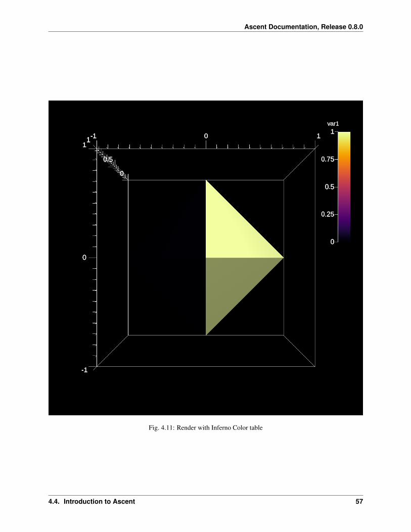
// the first scene (s2) will render a pseudocolor// plot using Inferno color tablescenes["s2/plots/p1/type"] = "pseudocolor";scenes["s2/plots/p1/field"] = "var1";scenes["s2/plots/p1/color_table/name"] = "Inferno";scenes["s2/image_name"] = "out_scene_ex4_render_inferno";
// print our full actions treestd::cout << actions.to_yaml() << std::endl;
// execute the actions
(continues on next page)
54 Chapter 4. Ascent Documentation

Ascent Documentation, Release 0.8.0
(continued from previous page)
a.execute(actions);
a.close();}
Python
import conduitimport conduit.blueprintimport ascentimport numpy as np
from ascent_tutorial_py_utils import tutorial_tets_example
mesh = conduit.Node()# (call helper to create example tet mesh as in blueprint example 2)tutorial_tets_example(mesh)
# Use Ascent to render pseudocolor plots with different color tablesa = ascent.Ascent()a.open()a.publish(mesh)
# setup actionsactions = conduit.Node()add_act = actions.append()add_act["action"] = "add_scenes"
# declare a two scenes (s1 and s2) to render the dataset# using different color tables## See the Color Tables docs for more details on what is supported:# https://ascent.readthedocs.io/en/latest/Actions/Scenes.html#color-tables#scenes = add_act["scenes"]
# the first scene (s1) will render a pseudocolor# plot using Viridis color tablescenes["s1/plots/p1/type"] = "pseudocolor";scenes["s1/plots/p1/field"] = "var1"scenes["s1/plots/p1/color_table/name"] = "Viridis"scenes["s1/image_name"] = "out_scene_ex4_render_viridis"
# the first scene (s2) will render a pseudocolor# plot using Inferno color tablescenes["s2/plots/p1/type"] = "pseudocolor"scenes["s2/plots/p1/field"] = "var1"scenes["s2/plots/p1/color_table/name"] = "Inferno"scenes["s2/image_name"] = "out_scene_ex4_render_inferno"
# print our full actions treeprint(actions.to_yaml())
# execute the actionsa.execute(actions)
(continues on next page)
4.4. Introduction to Ascent 55

Ascent Documentation, Release 0.8.0
(continued from previous page)
a.close()
Fig. 4.10: Render with Viridis Color table
4.4.5 Transforming data with Pipelines
Pipelines are the construct used to compose filters that transform the published input data into new meshes. This iswhere users specify typical geometric transforms (e.g., clipping and slicing), field based transforms (e.g., thresholdand contour), etc. The resulting data from each Pipeline can be used as input to Scenes or Extracts. Each pipelinecontains one or more filters that transform the published mesh data. See Ascent’s Scenes docs for deeper details on
56 Chapter 4. Ascent Documentation
Ascent Documentation, Release 0.8.0
Fig. 4.11: Render with Inferno Color table
4.4. Introduction to Ascent 57

Ascent Documentation, Release 0.8.0
Pipelines.
Calculating and rendering contours
C++
#include "ascent.hpp"#include "conduit_blueprint.hpp"
using namespace ascent;using namespace conduit;
int main(int argc, char **argv){
//create example mesh using the conduit blueprint braid helper
Node mesh;conduit::blueprint::mesh::examples::braid("hexs",
25,25,25,mesh);
// Use Ascent to calculate and render contours
Ascent a;
// open ascenta.open();
// publish mesh to ascenta.publish(mesh);
// setup actionsNode actions;Node &add_act = actions.append();add_act["action"] = "add_pipelines";Node &pipelines = add_act["pipelines"];
// create a pipeline (pl1) with a contour filter (f1)pipelines["pl1/f1/type"] = "contour";
// extract contours where braid variable// equals 0.2 and 0.4Node &contour_params = pipelines["pl1/f1/params"];contour_params["field"] = "braid";
double iso_vals[2] = {0.2, 0.4};contour_params["iso_values"].set(iso_vals,2);
// declare a scene to render the pipeline result
Node &add_act2 = actions.append();add_act2["action"] = "add_scenes";Node & scenes = add_act2["scenes"];
// add a scene (s1) with one pseudocolor plot (p1) that
(continues on next page)
58 Chapter 4. Ascent Documentation

Ascent Documentation, Release 0.8.0
(continued from previous page)
// will render the result of our pipeline (pl1)scenes["s1/plots/p1/type"] = "pseudocolor";scenes["s1/plots/p1/pipeline"] = "pl1";scenes["s1/plots/p1/field"] = "braid";// set the output file name (ascent will add ".png")scenes["s1/image_name"] = "out_pipeline_ex1_contour";
// print our full actions treestd::cout << actions.to_yaml() << std::endl;
// execute the actionsa.execute(actions);
a.close();}
Python
import conduitimport conduit.blueprintimport ascentimport numpy as np
mesh = conduit.Node()conduit.blueprint.mesh.examples.braid("hexs",
25,25,25,mesh)
# Use Ascent to calculate and render contoursa = ascent.Ascent()a.open()
# publish our mesh to ascenta.publish(mesh);
# setup actionsactions = conduit.Node()add_act = actions.append()add_act["action"] = "add_pipelines"pipelines = add_act["pipelines"]
# create a pipeline (pl1) with a contour filter (f1)pipelines["pl1/f1/type"] = "contour"
# extract contours where braid variable# equals 0.2 and 0.4contour_params = pipelines["pl1/f1/params"]contour_params["field"] = "braid"iso_vals = np.array([0.2, 0.4],dtype=np.float32)contour_params["iso_values"].set(iso_vals)
# declare a scene to render the pipeline result
(continues on next page)
4.4. Introduction to Ascent 59

Ascent Documentation, Release 0.8.0
(continued from previous page)
add_act2 = actions.append()add_act2["action"] = "add_scenes"scenes = add_act2["scenes"]
# add a scene (s1) with one pseudocolor plot (p1) that# will render the result of our pipeline (pl1)scenes["s1/plots/p1/type"] = "pseudocolor"scenes["s1/plots/p1/pipeline"] = "pl1"scenes["s1/plots/p1/field"] = "braid"# set the output file name (ascent will add ".png")scenes["s1/image_name"] = "out_pipeline_ex1_contour"
# print our full actions treeprint(actions.to_yaml())
# execute the actionsa.execute(actions)
a.close()
Combining threshold and clip transforms
C++
#include "ascent.hpp"#include "conduit_blueprint.hpp"
using namespace ascent;using namespace conduit;
int main(int argc, char **argv){
//create example mesh using the conduit blueprint braid helper
Node mesh;conduit::blueprint::mesh::examples::braid("hexs",
25,25,25,mesh);
// Use Ascent to calculate and render contours
Ascent a;
// open ascenta.open();
// publish mesh to ascenta.publish(mesh);
// setup actionsNode actions;Node &add_act = actions.append();add_act["action"] = "add_pipelines";
(continues on next page)
60 Chapter 4. Ascent Documentation

Ascent Documentation, Release 0.8.0
Fig. 4.12: Render of contour pipeline result
4.4. Introduction to Ascent 61

Ascent Documentation, Release 0.8.0
(continued from previous page)
Node &pipelines = add_act["pipelines"];
// create a pipeline (pl1) with a contour filter (f1)pipelines["pl1/f1/type"] = "contour";
// extract contours where braid variable// equals 0.2 and 0.4Node &contour_params = pipelines["pl1/f1/params"];contour_params["field"] = "braid";
double iso_vals[2] = {0.2, 0.4};contour_params["iso_values"].set(iso_vals,2);
// declare a scene to render the pipeline result
Node &add_act2 = actions.append();add_act2["action"] = "add_scenes";Node & scenes = add_act2["scenes"];
// add a scene (s1) with one pseudocolor plot (p1) that// will render the result of our pipeline (pl1)scenes["s1/plots/p1/type"] = "pseudocolor";scenes["s1/plots/p1/pipeline"] = "pl1";scenes["s1/plots/p1/field"] = "braid";// set the output file name (ascent will add ".png")scenes["s1/image_name"] = "out_pipeline_ex1_contour";
// print our full actions treestd::cout << actions.to_yaml() << std::endl;
// execute the actionsa.execute(actions);
a.close();}
Python
import conduitimport conduit.blueprintimport ascentimport numpy as np
mesh = conduit.Node()conduit.blueprint.mesh.examples.braid("hexs",
25,25,25,mesh)
# Use Ascent to calculate and render contoursa = ascent.Ascent()a.open()
# publish our mesh to ascent(continues on next page)
62 Chapter 4. Ascent Documentation

Ascent Documentation, Release 0.8.0
(continued from previous page)
a.publish(mesh);
# setup actionsactions = conduit.Node()add_act = actions.append()add_act["action"] = "add_pipelines"pipelines = add_act["pipelines"]
# create a pipeline (pl1) with a contour filter (f1)pipelines["pl1/f1/type"] = "contour"
# extract contours where braid variable# equals 0.2 and 0.4contour_params = pipelines["pl1/f1/params"]contour_params["field"] = "braid"iso_vals = np.array([0.2, 0.4],dtype=np.float32)contour_params["iso_values"].set(iso_vals)
# declare a scene to render the pipeline result
add_act2 = actions.append()add_act2["action"] = "add_scenes"scenes = add_act2["scenes"]
# add a scene (s1) with one pseudocolor plot (p1) that# will render the result of our pipeline (pl1)scenes["s1/plots/p1/type"] = "pseudocolor"scenes["s1/plots/p1/pipeline"] = "pl1"scenes["s1/plots/p1/field"] = "braid"# set the output file name (ascent will add ".png")scenes["s1/image_name"] = "out_pipeline_ex1_contour"
# print our full actions treeprint(actions.to_yaml())
# execute the actionsa.execute(actions)
a.close()
Creating and rendering the multiple pipelines
C++
#include "ascent.hpp"#include "conduit_blueprint.hpp"
using namespace ascent;using namespace conduit;
int main(int argc, char **argv){
//create example mesh using the conduit blueprint braid helper
Node mesh;
(continues on next page)
4.4. Introduction to Ascent 63

Ascent Documentation, Release 0.8.0
Fig. 4.13: Render of threshold and clip pipeline result
64 Chapter 4. Ascent Documentation

Ascent Documentation, Release 0.8.0
(continued from previous page)
conduit::blueprint::mesh::examples::braid("hexs",25,25,25,mesh);
// Use Ascent to calculate and render contours
Ascent a;
// open ascenta.open();
// publish mesh to ascenta.publish(mesh);
// setup actionsNode actions;Node &add_act = actions.append();add_act["action"] = "add_pipelines";Node &pipelines = add_act["pipelines"];
// create a pipeline (pl1) with a contour filter (f1)pipelines["pl1/f1/type"] = "contour";
// extract contours where braid variable// equals 0.2 and 0.4Node &contour_params = pipelines["pl1/f1/params"];contour_params["field"] = "braid";
double iso_vals[2] = {0.2, 0.4};contour_params["iso_values"].set(iso_vals,2);
// declare a scene to render the pipeline result
Node &add_act2 = actions.append();add_act2["action"] = "add_scenes";Node & scenes = add_act2["scenes"];
// add a scene (s1) with one pseudocolor plot (p1) that// will render the result of our pipeline (pl1)scenes["s1/plots/p1/type"] = "pseudocolor";scenes["s1/plots/p1/pipeline"] = "pl1";scenes["s1/plots/p1/field"] = "braid";// set the output file name (ascent will add ".png")scenes["s1/image_name"] = "out_pipeline_ex1_contour";
// print our full actions treestd::cout << actions.to_yaml() << std::endl;
// execute the actionsa.execute(actions);
a.close();}
Python
4.4. Introduction to Ascent 65

Ascent Documentation, Release 0.8.0
import conduitimport conduit.blueprintimport ascentimport numpy as np
mesh = conduit.Node()conduit.blueprint.mesh.examples.braid("hexs",
25,25,25,mesh)
# Use Ascent to calculate and render contoursa = ascent.Ascent()a.open()
# publish our mesh to ascenta.publish(mesh);
# setup actionsactions = conduit.Node()add_act = actions.append()add_act["action"] = "add_pipelines"pipelines = add_act["pipelines"]
# create a pipeline (pl1) with a contour filter (f1)pipelines["pl1/f1/type"] = "contour"
# extract contours where braid variable# equals 0.2 and 0.4contour_params = pipelines["pl1/f1/params"]contour_params["field"] = "braid"iso_vals = np.array([0.2, 0.4],dtype=np.float32)contour_params["iso_values"].set(iso_vals)
# declare a scene to render the pipeline result
add_act2 = actions.append()add_act2["action"] = "add_scenes"scenes = add_act2["scenes"]
# add a scene (s1) with one pseudocolor plot (p1) that# will render the result of our pipeline (pl1)scenes["s1/plots/p1/type"] = "pseudocolor"scenes["s1/plots/p1/pipeline"] = "pl1"scenes["s1/plots/p1/field"] = "braid"# set the output file name (ascent will add ".png")scenes["s1/image_name"] = "out_pipeline_ex1_contour"
# print our full actions treeprint(actions.to_yaml())
# execute the actionsa.execute(actions)
a.close()
66 Chapter 4. Ascent Documentation

Ascent Documentation, Release 0.8.0
Fig. 4.14: Render of multiple pipeline results
4.4. Introduction to Ascent 67

Ascent Documentation, Release 0.8.0
4.4.6 Capturing data with Extracts
Extracts are the construct that allows users to capture and process data outside Ascent’s pipeline infrastructure. Extractuse cases include: Saving mesh data to HDF5 files, creating Cinema databases, and running custom Python analysisscripts. These examples outline how to use several of Ascent’s extracts. See Ascent’s Extracts docs for deeper detailson Extracts.
Exporting input mesh data to Blueprint HDF5 files
Related docs: Relay
C++
#include <iostream>#include "ascent.hpp"#include "conduit_blueprint.hpp"
using namespace ascent;using namespace conduit;
int main(int argc, char **argv){
//create example mesh using the conduit blueprint braid helper
Node mesh;conduit::blueprint::mesh::examples::braid("hexs",
25,25,25,mesh);
// Use Ascent to export our mesh to blueprint flavored hdf5 filesAscent a;
// open ascenta.open();
// publish mesh to ascenta.publish(mesh);
// setup actionsNode actions;Node &add_act = actions.append();add_act["action"] = "add_extracts";
// add a relay extract that will write mesh data to// blueprint hdf5 filesNode &extracts = add_act["extracts"];extracts["e1/type"] = "relay";extracts["e1/params/path"] = "out_export_braid_all_fields";extracts["e1/params/protocol"] = "blueprint/mesh/hdf5";
// print our full actions treestd::cout << actions.to_yaml() << std::endl;
// execute the actionsa.execute(actions);
(continues on next page)
68 Chapter 4. Ascent Documentation

Ascent Documentation, Release 0.8.0
(continued from previous page)
// close ascenta.close();
}
Python
import conduitimport conduit.blueprintimport ascentimport numpy as np
mesh = conduit.Node()conduit.blueprint.mesh.examples.braid("hexs",
25,25,25,mesh)
# Use Ascent to export our mesh to blueprint flavored hdf5 filesa = ascent.Ascent()a.open()
# publish mesh to ascenta.publish(mesh)
# setup actionsactions = conduit.Node()add_act = actions.append()add_act["action"] = "add_extracts"
# add a relay extract that will write mesh data to# blueprint hdf5 filesextracts = add_act["extracts"]extracts["e1/type"] = "relay"extracts["e1/params/path"] = "out_export_braid_all_fields"extracts["e1/params/protocol"] = "blueprint/mesh/hdf5"
# print our full actions treeprint(actions.to_yaml())
# execute the actionsa.execute(actions)
# close ascenta.close()
How can you use these files?
You can use them as input to Ascent Replay, which allows you to run Ascent outside of a simulation code.
You can also visualize meshes from these files using VisIt 2.13 or newer.
VisIt can also export Blueprint HDF5 files, which can be used as input to Ascent Replay.
Blueprint files help bridge in situ and post hoc workflows.
4.4. Introduction to Ascent 69

Ascent Documentation, Release 0.8.0
Fig. 4.15: Exported Mesh Rendered in VisIt
70 Chapter 4. Ascent Documentation

Ascent Documentation, Release 0.8.0
Exporting selected fields from input mesh data to Blueprint HDF5 files
Related docs: Relay
C++
#include <iostream>#include "ascent.hpp"#include "conduit_blueprint.hpp"
using namespace ascent;using namespace conduit;
int main(int argc, char **argv){
//create example mesh using the conduit blueprint braid helper
Node mesh;conduit::blueprint::mesh::examples::braid("hexs",
25,25,25,mesh);
// Use Ascent to export our mesh to blueprint flavored hdf5 filesAscent a;
// open ascenta.open();
// publish mesh to ascenta.publish(mesh);
// setup actionsNode actions;Node &add_act = actions.append();add_act["action"] = "add_extracts";
// add a relay extract that will write mesh data to// blueprint hdf5 filesNode &extracts = add_act["extracts"];extracts["e1/type"] = "relay";extracts["e1/params/path"] = "out_export_braid_one_field";extracts["e1/params/protocol"] = "blueprint/mesh/hdf5";
//// add fields parameter to limit the export to the just// the `braid` field//extracts["e1/params/fields"].append().set("braid");
// print our full actions treestd::cout << actions.to_yaml() << std::endl;
// execute the actionsa.execute(actions);
// close ascent
(continues on next page)
4.4. Introduction to Ascent 71

Ascent Documentation, Release 0.8.0
(continued from previous page)
a.close();}
Python
import conduitimport conduit.blueprintimport ascentimport numpy as np
mesh = conduit.Node()conduit.blueprint.mesh.examples.braid("hexs",
25,25,25,mesh)
# Use Ascent to export our mesh to blueprint flavored hdf5 filesa = ascent.Ascent()a.open()
# publish mesh to ascenta.publish(mesh);
# setup actionsactions = conduit.Node()add_act = actions.append()add_act["action"] = "add_extracts"
# add a relay extract that will write mesh data to# blueprint hdf5 filesextracts = add_act["extracts"]extracts["e1/type"] = "relay"extracts["e1/params/path"] = "out_export_braid_one_field"extracts["e1/params/protocol"] = "blueprint/mesh/hdf5"
## add fields parameter to limit the export to the just# the `braid` field#extracts["e1/params/fields"].append().set("braid")
# print our full actions treeprint(actions.to_yaml())
# execute the actionsa.execute(actions);
a.close()
Exporting the result of a pipeline to Blueprint HDF5 files
Related docs: Relay
72 Chapter 4. Ascent Documentation

Ascent Documentation, Release 0.8.0
Fig. 4.16: Exported Mesh Rendered in VisIt
4.4. Introduction to Ascent 73

Ascent Documentation, Release 0.8.0
C++
#include <iostream>#include "ascent.hpp"#include "conduit_blueprint.hpp"
using namespace ascent;using namespace conduit;
int main(int argc, char **argv){
//create example mesh using the conduit blueprint braid helper
Node mesh;conduit::blueprint::mesh::examples::braid("hexs",
25,25,25,mesh);
// Use Ascent to export contours to blueprint flavored hdf5 filesAscent a;
// open ascenta.open();
// publish mesh to ascenta.publish(mesh);
// setup actionsNode actions;Node &add_act = actions.append();add_act["action"] = "add_pipelines";Node &pipelines = add_act["pipelines"];
// create a pipeline (pl1) with a contour filter (f1)pipelines["pl1/f1/type"] = "contour";
// extract contours where braid variable// equals 0.2 and 0.4Node &contour_params = pipelines["pl1/f1/params"];contour_params["field"] = "braid";
double iso_vals[2] = {0.2, 0.4};contour_params["iso_values"].set(iso_vals,2);
// add an extract to capture the pipeline resultNode &add_act2 = actions.append();add_act2["action"] = "add_extracts";Node &extracts = add_act2["extracts"];
// add an relay extract (e1) to export the pipeline result// (pl1) to blueprint hdf5 filesextracts["e1/type"] = "relay";extracts["e1/pipeline"] = "pl1";extracts["e1/params/path"] = "out_extract_braid_contour";extracts["e1/params/protocol"] = "blueprint/mesh/hdf5";
(continues on next page)
74 Chapter 4. Ascent Documentation

Ascent Documentation, Release 0.8.0
(continued from previous page)
// print our full actions treestd::cout << actions.to_yaml() << std::endl;
// execute the actionsa.execute(actions);
// close ascenta.close();
}
Python
import conduitimport conduit.blueprintimport ascentimport numpy as np
mesh = conduit.Node()conduit.blueprint.mesh.examples.braid("hexs",
25,25,25,mesh)
# Use Ascent to calculate and render contoursa = ascent.Ascent()a.open()
# publish our mesh to ascenta.publish(mesh);
# setup actionsactions = conduit.Node()add_act = actions.append();add_act["action"] = "add_pipelines"pipelines = add_act["pipelines"]
# create a pipeline (pl1) with a contour filter (f1)pipelines["pl1/f1/type"] = "contour"
# extract contours where braid variable# equals 0.2 and 0.4contour_params = pipelines["pl1/f1/params"]contour_params["field"] = "braid"iso_vals = np.array([0.2, 0.4],dtype=np.float32)contour_params["iso_values"].set(iso_vals)
# add an extract to capture the pipeline resultadd_act2 = actions.append()add_act2["action"] = "add_extracts"extracts = add_act2["extracts"]
# add an relay extract (e1) to export the pipeline result# (pl1) to blueprint hdf5 filesextracts["e1/type"] = "relay"
(continues on next page)
4.4. Introduction to Ascent 75

Ascent Documentation, Release 0.8.0
(continued from previous page)
extracts["e1/pipeline"] = "pl1"extracts["e1/params/path"] = "out_extract_braid_contour"extracts["e1/params/protocol"] = "blueprint/mesh/hdf5"
# print our full actions treeprint(actions.to_yaml())
# execute the actionsa.execute(actions);
a.close()
Fig. 4.17: Exported Mesh Rendered in VisIt
76 Chapter 4. Ascent Documentation

Ascent Documentation, Release 0.8.0
Creating a Cinema image database for post-hoc exploration
Related docs: Cinema Databases
C++
#include <iostream>#include "ascent.hpp"#include "conduit_blueprint.hpp"
using namespace ascent;using namespace conduit;
int main(int argc, char **argv){
//create example mesh using the conduit blueprint braid helper
Node mesh;conduit::blueprint::mesh::examples::braid("hexs",
25,25,25,mesh);
// Use Ascent to create a Cinema Image DatabaseAscent a;
// open ascenta.open();
// publish mesh to ascenta.publish(mesh);
// setup actionsNode actions;Node &add_act = actions.append();add_act["action"] = "add_pipelines";Node &pipelines = add_act["pipelines"];
// create a pipeline (pl1) with a contour filter (f1)pipelines["pl1/f1/type"] = "contour";
// extract contours where braid variable// equals 0.2 and 0.4Node &contour_params = pipelines["pl1/f1/params"];contour_params["field"] = "braid";
double iso_vals[2] = {0.2, 0.4};contour_params["iso_values"].set(iso_vals,2);
// declare a scene to render several angles of// the pipeline result (pl1) to a Cinema Image// database
Node &add_act2 = actions.append();add_act2["action"] = "add_scenes";Node &scenes = add_act2["scenes"];
(continues on next page)
4.4. Introduction to Ascent 77

Ascent Documentation, Release 0.8.0
(continued from previous page)
scenes["s1/plots/p1/type"] = "pseudocolor";scenes["s1/plots/p1/pipeline"] = "pl1";scenes["s1/plots/p1/field"] = "braid";// select cinema pathscenes["s1/renders/r1/type"] = "cinema";// use 5 renders in phiscenes["s1/renders/r1/phi"] = 5;// and 5 renders in thetascenes["s1/renders/r1/theta"] = 5;// setup to output database to:// cinema_databases/out_extract_cinema_contour// you can view using a webserver to open:// cinema_databases/out_extract_cinema_contour/index.htmlscenes["s1/renders/r1/db_name"] = "out_extract_cinema_contour";
// print our full actions treestd::cout << actions.to_yaml() << std::endl;
// execute the actionsa.execute(actions);
// close ascenta.close();
}
Python
import conduitimport conduit.blueprintimport ascentimport numpy as np
mesh = conduit.Node()conduit.blueprint.mesh.examples.braid("hexs",
25,25,25,mesh)
a = ascent.Ascent()a.open()
# publish mesh to ascenta.publish(mesh);
# setup actionsactions = conduit.Node()add_act = actions.append();add_act["action"] = "add_pipelines"pipelines = add_act["pipelines"]
# create a pipeline (pl1) with a contour filter (f1)pipelines["pl1/f1/type"] = "contour"
# extract contours where braid variable(continues on next page)
78 Chapter 4. Ascent Documentation

Ascent Documentation, Release 0.8.0
(continued from previous page)
# equals 0.2 and 0.4contour_params = pipelines["pl1/f1/params"]contour_params["field"] = "braid"iso_vals = np.array([0.2, 0.4],dtype=np.float32)contour_params["iso_values"].set(iso_vals)
# declare a scene to render several angles of# the pipeline result (pl1) to a Cinema Image# database
add_act2 = actions.append()add_act2["action"] = "add_scenes"scenes = add_act2["scenes"]
scenes["s1/plots/p1/type"] = "pseudocolor"scenes["s1/plots/p1/pipeline"] = "pl1"scenes["s1/plots/p1/field"] = "braid"# select cinema pathscenes["s1/renders/r1/type"] = "cinema"# use 5 renders in phiscenes["s1/renders/r1/phi"] = 5# and 5 renders in thetascenes["s1/renders/r1/theta"] = 5# setup to output database to:# cinema_databases/out_extract_cinema_contour# you can view using a webserver to open:# cinema_databases/out_extract_cinema_contour/index.htmlscenes["s1/renders/r1/db_name"] = "out_extract_cinema_contour"
# print our full actions treeprint(actions.to_yaml())
# execute the actionsa.execute(actions);
a.close()
Fig. 4.18: Snapshot of Cinema Database Result
4.4. Introduction to Ascent 79

Ascent Documentation, Release 0.8.0
Using a Python Extract to execute custom Python analysis
Related docs: Python
C++
#include <iostream>#include "ascent.hpp"#include "conduit_blueprint.hpp"
using namespace ascent;using namespace conduit;
int main(int argc, char **argv){
//create example mesh using the conduit blueprint braid helper
Node mesh;conduit::blueprint::mesh::examples::braid("hexs",
25,25,25,mesh);
// Use Ascent to execute a python script// that computes a histogramAscent a;
// open ascenta.open();
// publish mesh to ascenta.publish(mesh);
// setup actionsNode actions;Node &add_act = actions.append();add_act["action"] = "add_extracts";
// add an extract to execute custom python code// in `ascent_tutorial_python_extract_braid_histogram.py`
//// This extract script runs the same histogram code as above,// but saves the output to `out_py_extract_hist_results.yaml`//
Node &extracts = add_act["extracts"];extracts["e1/type"] = "python";extracts["e1/params/file"] = "ascent_tutorial_python_extract_braid_histogram.py";
// print our full actions treestd::cout << actions.to_yaml() << std::endl;
// execute the actionsa.execute(actions);
// close ascent
(continues on next page)
80 Chapter 4. Ascent Documentation

Ascent Documentation, Release 0.8.0
(continued from previous page)
a.close();
}
Output
Energy extents: -9.850344080110776 9.956328748632988
Histogram of Energy:
Counts:[ 13 23 33 55 85 102 135 153 220 211 254 267 312 339 365 377 428 486555 537 594 635 681 683 685 688 635 606 629 530 475 480 474 466 360 366349 284 243 202 167 120 104 72 60 45 21 11 10]
Bin Edges:[-9.85034408 -9.44612627 -9.04190845 -8.63769064 -8.23347283 -7.82925502-7.4250372 -7.02081939 -6.61660158 -6.21238376 -5.80816595 -5.40394814-4.99973033 -4.59551251 -4.1912947 -3.78707689 -3.38285907 -2.97864126-2.57442345 -2.17020564 -1.76598782 -1.36177001 -0.9575522 -0.55333438-0.14911657 0.25510124 0.65931905 1.06353687 1.46775468 1.871972492.2761903 2.68040812 3.08462593 3.48884374 3.89306156 4.297279374.70149718 5.10571499 5.50993281 5.91415062 6.31836843 6.722586257.12680406 7.53102187 7.93523968 8.3394575 8.74367531 9.147893129.55211094 9.95632875]
Python
import conduitimport conduit.blueprintimport ascentimport numpy as np
mesh = conduit.Node()conduit.blueprint.mesh.examples.braid("hexs",
25,25,25,mesh)
## Ascent provides an embedded Python environment to support# custom analysis. When using MPI this environment supports# distributed-memory processing with one Python interpreter# per MPI task.## You can use this environment in Ascent's Python Extract.## In the case you are already using Ascent from Python this may# appear a bit odd. Yes, this feature is most useful to# provide a Python analysis environment to simulation codes written# in other lanauges (C++, C, or Fortran). Reguardless, we can# still access it and leverage it from Python.##
(continues on next page)
4.4. Introduction to Ascent 81

Ascent Documentation, Release 0.8.0
(continued from previous page)
# For more detials about the Python extract, see:# https://ascent.readthedocs.io/en/latest/Actions/Extracts.html#python#
## First, we a histogram calcuation directly in our current# Python interpreter and then we will compare results# with running the same code via a Python Extract.#
# fetch the numpy array for the braid field valuese_vals = mesh["fields/braid/values"]
# find the data extents of the braid fielde_min, e_max = e_vals.min(), e_vals.max()
# compute bins on extentsbins = np.linspace(e_min, e_max)
# get histogram countshist, bin_edges = np.histogram(e_vals, bins = bins)
print("\nEnergy extents: {} {}\n".format(e_min, e_max))print("Histogram of Energy:\n")print("Counts:")print(hist)print("\nBin Edges:")print(bin_edges)print("")
# save our results to a yaml filehist_results = conduit.Node()hist_results["hist"] = histhist_results["bin_edges"] = bin_edgeshist_results.save("out_hist_results.yaml","yaml")
# Use Ascent to execute the histogram script.a = ascent.Ascent()ascent_opts = conduit.Node()ascent_opts["exceptions"] = "forward"a.open(ascent_opts)
# publish mesh to ascenta.publish(mesh);
# setup actionsactions = conduit.Node()add_act = actions.append()add_act["action"] = "add_extracts"
# add an extract to execute custom python code# in `ascent_tutorial_python_extract_braid_histogram.py`
## This extract script runs the same histogram code as above,# but saves the output to `out_py_extract_hist_results.yaml`#
(continues on next page)
82 Chapter 4. Ascent Documentation

Ascent Documentation, Release 0.8.0
(continued from previous page)
extracts = add_act["extracts"]extracts["e1/type"] = "python"extracts["e1/params/file"] = "ascent_tutorial_python_extract_braid_histogram.py"
# print our full actions treeprint(actions.to_yaml())
# execute the actionsa.execute(actions);
# close ascenta.close()
## Load and compare the extract yaml results,# they should match our earlier results.#hist_extract_results = conduit.Node()hist_extract_results.load("out_py_extract_hist_results.yaml",protocol="yaml")
diff_info = conduit.Node()# hist_results is a Node with our earlier resultsif hist_results.diff(hist_extract_results,diff_info):
print("Extract results differ!")print(diff_info.to_yaml())
else:print("Extract results match.")
Output
Energy extents: -9.850344080110776 9.956328748632988
Histogram of Energy:
Counts:[ 13 23 33 55 85 102 135 153 220 211 254 267 312 339 365 377 428 486555 537 594 635 681 683 685 688 635 606 629 530 475 480 474 466 360 366349 284 243 202 167 120 104 72 60 45 21 11 10]
Bin Edges:[-9.85034408 -9.44612627 -9.04190845 -8.63769064 -8.23347283 -7.82925502-7.4250372 -7.02081939 -6.61660158 -6.21238376 -5.80816595 -5.40394814-4.99973033 -4.59551251 -4.1912947 -3.78707689 -3.38285907 -2.97864126-2.57442345 -2.17020564 -1.76598782 -1.36177001 -0.9575522 -0.55333438-0.14911657 0.25510124 0.65931905 1.06353687 1.46775468 1.871972492.2761903 2.68040812 3.08462593 3.48884374 3.89306156 4.297279374.70149718 5.10571499 5.50993281 5.91415062 6.31836843 6.722586257.12680406 7.53102187 7.93523968 8.3394575 8.74367531 9.147893129.55211094 9.95632875]
-action: "add_extracts"extracts:e1:
(continues on next page)
4.4. Introduction to Ascent 83

Ascent Documentation, Release 0.8.0
(continued from previous page)
type: "python"params:
file: "ascent_tutorial_python_extract_braid_histogram.py"
Energy extents: -9.850344080110776 9.956328748632988
Histogram of Energy:
Counts:[ 13 23 33 55 85 102 135 153 220 211 254 267 312 339 365 377 428 486555 537 594 635 681 683 685 688 635 606 629 530 475 480 474 466 360 366349 284 243 202 167 120 104 72 60 45 21 11 10]
Bin Edges:[-9.85034408 -9.44612627 -9.04190845 -8.63769064 -8.23347283 -7.82925502-7.4250372 -7.02081939 -6.61660158 -6.21238376 -5.80816595 -5.40394814-4.99973033 -4.59551251 -4.1912947 -3.78707689 -3.38285907 -2.97864126-2.57442345 -2.17020564 -1.76598782 -1.36177001 -0.9575522 -0.55333438-0.14911657 0.25510124 0.65931905 1.06353687 1.46775468 1.871972492.2761903 2.68040812 3.08462593 3.48884374 3.89306156 4.297279374.70149718 5.10571499 5.50993281 5.91415062 6.31836843 6.722586257.12680406 7.53102187 7.93523968 8.3394575 8.74367531 9.147893129.55211094 9.95632875]
Extract results match.
4.4.7 Asking and answering questions with Queries
Queries are a way to ask summarization questions about meshes. Queries results can be used with Triggers to adaptanalysis and visualization actions. This section shows how to execute queries with Ascent and access query results.See Queries docs for deeper details on Queries.
Extracting mesh cycle and entropy of a time varying mesh
C++
#include <iostream>#include <sstream>
#include "ascent.hpp"#include "conduit_blueprint.hpp"
#include "ascent_tutorial_cpp_utils.hpp"
using namespace ascent;using namespace conduit;
int main(int argc, char **argv){
// Use Ascent to extract mesh cycle and entropy of a time varying meshAscent a;
// open ascent(continues on next page)
84 Chapter 4. Ascent Documentation

Ascent Documentation, Release 0.8.0
(continued from previous page)
a.open();
// setup actionsNode actions;Node &add_act = actions.append();add_act["action"] = "add_queries";
// declare a queries to ask some questionsNode &queries = add_act["queries"] ;
// add a simple query expression (q1)queries["q1/params/expression"] = "cycle()";;queries["q1/params/name"] = "cycle";
// add a more complex query expression (q2)queries["q2/params/expression"] = "entropy(histogram(field('gyre'), num_bins=128))
→˓";queries["q2/params/name"] = "entropy_of_gyre";
// declare a scene to render the datasetNode &add_scenes = actions.append();add_scenes["action"] = "add_scenes";Node &scenes = add_scenes["scenes"];scenes["s1/plots/p1/type"] = "pseudocolor";scenes["s1/plots/p1/field"] = "gyre";// Set the output file name (ascent will add ".png")scenes["s1/image_name"] = "out_gyre";
// print our full actions treestd::cout << actions.to_yaml() << std::endl;
// gyre time varying paramsint nsteps = 10;float time_value = 0.0;float delta_time = 0.5;
Node mesh;Node info;
for( int step =0; step < nsteps; step++){
// call helper that generates a gyre time varying example mesh.// gyre ref :https://shaddenlab.berkeley.edu/uploads/LCS-tutorial/examples.
→˓htmltutorial_gyre_example(time_value, mesh);
// update the example cycleint cycle = 100 + step * 100;mesh["state/cycle"] = cycle;std::cout << "time: " << time_value << " cycle: " << cycle << std::endl;
// publish mesh to ascenta.publish(mesh);
// update image namestd::ostringstream oss;oss << "out_gyre_" << std::setfill('0') << std::setw(4) << step;
(continues on next page)
4.4. Introduction to Ascent 85

Ascent Documentation, Release 0.8.0
(continued from previous page)
scenes["s1/image_name"] = oss.str();
// execute the actionsa.execute(actions);
// retrieve the info node that contains the query resultsNode ts_info;a.info(ts_info);
// add to our running infoinfo["expressions"].update(ts_info["expressions"]);
// update timetime_value = time_value + delta_time;
}
// close ascenta.close();
// view the results of the cycle querystd::cout << info["expressions/cycle"].to_yaml() << std::endl;// Note that query results can be indexed by cycle
// view the results of the cycle querystd::cout << info["expressions/entropy_of_gyre"].to_yaml() << std::endl;
// create an array with the entropy values from all// cyclesNode entropy;entropy.set(DataType::float64(nsteps));float64 *entropy_vals_ptr = entropy.value();
// get the node that has the time historyNode &gyre = info["expressions/entropy_of_gyre"];
// reformat conduit data into summary arrayfor(int i=i; i < gyre.number_of_children(); i++ ){
entropy_vals_ptr[i] = gyre[i]["value"].to_float64();}
std::cout << "Entropy Result" << std::endl;std::cout << entropy.to_yaml() << std::endl;
}
Python
import conduitimport conduit.blueprintimport ascentimport numpy as np
from ascent_tutorial_py_utils import tutorial_gyre_example
# Use Ascent to extract mesh cycle and entropy of a time varying mesha = ascent.Ascent()
(continues on next page)
86 Chapter 4. Ascent Documentation

Ascent Documentation, Release 0.8.0
(continued from previous page)
a.open()
# setup actionsactions = conduit.Node()add_act = actions.append()add_act["action"] = "add_queries"
# declare a queries to ask some questionsqueries = add_act["queries"]
# add a simple query expression (q1)queries["q1/params/expression"] = "cycle()"queries["q1/params/name"] = "cycle"
# add a more complex query expression (q2)queries["q2/params/expression"] = "entropy(histogram(field('gyre'), num_bins=128))"queries["q2/params/name"] = "entropy_of_gyre"
# declare a scene to render the datasetadd_scenes = actions.append()add_scenes["action"] = "add_scenes"scenes = add_scenes["scenes"]scenes["s1/plots/p1/type"] = "pseudocolor"scenes["s1/plots/p1/field"] = "gyre"# Set the output file name (ascent will add ".png")scenes["s1/image_name"] = "out_gyre"
# view our full actions treeprint(actions.to_yaml())
# gyre time varying paramsnsteps = 10time = 0.0delta_time = 0.5
info = conduit.Node()for step in range(nsteps):
# call helper that generates a gyre time varying example mesh.# gyre ref :https://shaddenlab.berkeley.edu/uploads/LCS-tutorial/examples.htmlmesh = tutorial_gyre_example(time)
# update the example cyclecycle = 100 + step * 100mesh["state/cycle"] = cycleprint("time: {} cycle: {}".format(time,cycle))
# publish mesh to ascenta.publish(mesh)
# update image namescenes["s1/image_name"] = "out_gyre_%04d" % step;
# execute the actionsa.execute(actions)
# retrieve the info node that contains the query resultsts_info = conduit.Node()
(continues on next page)
4.4. Introduction to Ascent 87

Ascent Documentation, Release 0.8.0
(continued from previous page)
a.info(ts_info)
# add to our running infoinfo["expressions"].update(ts_info["expressions"])
# update timetime = time + delta_time
# close ascenta.close()
# view the results of the cycle queryprint(info["expressions/cycle"].to_yaml())# Note that query results can be indexed by cycle
# view the results of the cycle queryprint(info["expressions/entropy_of_gyre"].to_yaml())
# create an array with the entropy values from all# cyclesentropy = np.zeros(nsteps)# get the node that has the time historygyre = info["expressions/entropy_of_gyre"]
# transfer conduit data to our summary numpy arrayfor i in range(gyre.number_of_children()):
entropy[i] = gyre[i]["value"]
print("Entropy Result")print(entropy)
Output
-action: "add_queries"queries:q1:
params:expression: "cycle()"name: "cycle"
q2:params:
expression: "entropy(histogram(field('gyre'), num_bins=128))"name: "entropy_of_gyre"
-action: "add_scenes"scenes:s1:
plots:p1:type: "pseudocolor"field: "gyre"
image_name: "out_gyre"
time: 0.0 cycle: 100time: 0.5 cycle: 200
(continues on next page)
88 Chapter 4. Ascent Documentation

Ascent Documentation, Release 0.8.0
(continued from previous page)
time: 1.0 cycle: 300time: 1.5 cycle: 400time: 2.0 cycle: 500time: 2.5 cycle: 600time: 3.0 cycle: 700time: 3.5 cycle: 800time: 4.0 cycle: 900time: 4.5 cycle: 1000
100:type: "int"value: 100
200:type: "int"value: 200
300:type: "int"value: 300
400:type: "int"value: 400
500:type: "int"value: 500
600:type: "int"value: 600
700:type: "int"value: 700
800:type: "int"value: 800
900:type: "int"value: 900
1000:type: "int"value: 1000
100:value: 3.81580590726479type: "double"
200:value: 4.43027379899862type: "double"
300:value: 4.42357515605932type: "double"
400:value: 4.4133821818731type: "double"
500:value: 4.40290017527564type: "double"
600:(continues on next page)
4.4. Introduction to Ascent 89

Ascent Documentation, Release 0.8.0
(continued from previous page)
value: 4.3643209637501type: "double"
700:value: 4.40290017527564type: "double"
800:value: 4.4133821818731type: "double"
900:value: 4.42357515605932type: "double"
1000:value: 4.43027379899862type: "double"
Entropy Result[3.81580591 4.4302738 4.42357516 4.41338218 4.40290018 4.364320964.40290018 4.41338218 4.42357516 4.4302738 ]
4.4.8 Adapting visualization with Triggers
Triggers allow the user to specify a set of actions that are triggered by the result of a boolean expression. They provideflexibility to adapt what analysis and visualization actions are taken in situ. Triggers leverage Ascent’s Query andExpression infrastructure. See Ascent’s Triggers docs for deeper details on Triggers.
Using triggers to render when events occur
C++
#include <iostream>#include <sstream>
#include "ascent.hpp"#include "conduit_blueprint.hpp"
#include "ascent_tutorial_cpp_utils.hpp"
using namespace ascent;using namespace conduit;
int main(int argc, char **argv){
// Use triggers to render when conditions occurAscent a;
// open ascenta.open();
// setup actionsNode actions;
// declare a question to askNode &add_queries = actions.append();add_queries["action"] = "add_queries";
(continues on next page)
90 Chapter 4. Ascent Documentation

Ascent Documentation, Release 0.8.0
(continued from previous page)
// add our entropy query (q1)Node &queries = add_queries["queries"];queries["q1/params/expression"] = "entropy(histogram(field('gyre'), num_bins=128))
→˓";queries["q1/params/name"] = "entropy";
// declare triggersNode &add_triggers = actions.append();add_triggers["action"] = "add_triggers";Node &triggers = add_triggers["triggers"];
// add a simple trigger (t1_ that fires at cycle 500triggers["t1/params/condition"] = "cycle() == 500";triggers["t1/params/actions_file"] = "cycle_trigger_actions.yaml";
// add trigger (t2) that fires when the change in entroy exceeds 0.5
// the history function allows you to access query results of previous// cycles. relative_index indicates how far back in history to look.
// Looking at the plot of gyre entropy in the previous notebook, we see a jump// in entropy at cycle 200, so we expect the trigger to fire at cycle 200triggers["t2/params/condition"] = "entropy - history(entropy, relative_index = 1)
→˓> 0.5";triggers["t2/params/actions_file"] = "entropy_trigger_actions.yaml";
// print our full actions treestd::cout << actions.to_yaml() << std::endl;
// gyre time varying paramsint nsteps = 10;float time_value = 0.0;float delta_time = 0.5;
Node mesh;
for( int step =0; step < nsteps; step++){
// call helper that generates a gyre time varying example mesh.// gyre ref :https://shaddenlab.berkeley.edu/uploads/LCS-tutorial/examples.
→˓htmltutorial_gyre_example(time_value, mesh);
// update the example cycleint cycle = 100 + step * 100;mesh["state/cycle"] = cycle;std::cout << "time: " << time_value << " cycle: " << cycle << std::endl;
// publish mesh to ascenta.publish(mesh);
// execute the actionsa.execute(actions);
// update timetime_value = time_value + delta_time;
(continues on next page)
4.4. Introduction to Ascent 91

Ascent Documentation, Release 0.8.0
(continued from previous page)
}// retrieve the info node that contains the query resultsNode info;a.info(info);
// close ascenta.close();
// this will render:// cycle_trigger_out_500.png// entropy_trigger_out_200.png////// We can also examine when the triggers executed by looking at the expressions// results in the output info//
std::cout << info["expressions"].to_yaml() << std::endl;}
Python
import conduitimport conduit.blueprintimport ascentimport numpy as np
from ascent_tutorial_py_utils import tutorial_gyre_example
# Use triggers to render when conditions occura = ascent.Ascent()a.open()
# setup actionsactions = conduit.Node()
# declare a question to askadd_queries = actions.append()add_queries["action"] = "add_queries"
# add our entropy query (q1)queries = add_queries["queries"]queries["q1/params/expression"] = "entropy(histogram(field('gyre'), num_bins=128))"queries["q1/params/name"] = "entropy"
# declare triggersadd_triggers = actions.append()add_triggers["action"] = "add_triggers"triggers = add_triggers["triggers"]
# add a simple trigger (t1_ that fires at cycle 500triggers["t1/params/condition"] = "cycle() == 500"triggers["t1/params/actions_file"] = "cycle_trigger_actions.yaml"
# add trigger (t2) that fires when the change in entroy exceeds 0.5
(continues on next page)
92 Chapter 4. Ascent Documentation

Ascent Documentation, Release 0.8.0
(continued from previous page)
# the history function allows you to access query results of previous# cycles. relative_index indicates how far back in history to look.
# Looking at the plot of gyre entropy in the previous notebook, we see a jump# in entropy at cycle 200, so we expect the trigger to fire at cycle 200triggers["t2/params/condition"] = "entropy - history(entropy, relative_index = 1) > 0.→˓5"triggers["t2/params/actions_file"] = "entropy_trigger_actions.yaml"
# view our full actions treeprint(actions.to_yaml())
# gyre time varying paramsnsteps = 10time = 0.0delta_time = 0.5
for step in range(nsteps):# call helper that generates a double gyre time varying example mesh.# gyre ref :https://shaddenlab.berkeley.edu/uploads/LCS-tutorial/examples.htmlmesh = tutorial_gyre_example(time)
# update the example cyclecycle = 100 + step * 100mesh["state/cycle"] = cycleprint("time: {} cycle: {}".format(time,cycle))
# publish mesh to ascenta.publish(mesh)
# execute the actionsa.execute(actions)
# update timetime = time + delta_time
# retrieve the info node that contains the trigger and query resultsinfo = conduit.Node()a.info(info)
# close ascenta.close()
# this will render:# cycle_trigger_out_500.png# entropy_trigger_out_200.png
## We can also examine when the triggers executed by looking at the expressions# results in the output info#print(info["expressions"].to_yaml())
Output
-(continues on next page)
4.4. Introduction to Ascent 93

Ascent Documentation, Release 0.8.0
(continued from previous page)
action: "add_queries"queries:q1:
params:expression: "entropy(histogram(field('gyre'), num_bins=128))"name: "entropy"
-action: "add_triggers"triggers:t1:
params:condition: "cycle() == 500"actions_file: "cycle_trigger_actions.yaml"
t2:params:
condition: "entropy - history(entropy, relative_index = 1) > 0.5"actions_file: "entropy_trigger_actions.yaml"
time: 0 cycle: 100time: 0.5 cycle: 200time: 1 cycle: 300time: 1.5 cycle: 400time: 2 cycle: 500time: 2.5 cycle: 600time: 3 cycle: 700time: 3.5 cycle: 800time: 4 cycle: 900time: 4.5 cycle: 1000
entropy:100:value: 3.81580590726479type: "double"
200:value: 4.43027379899862type: "double"
300:value: 4.42357515605932type: "double"
400:value: 4.4133821818731type: "double"
500:value: 4.40290017527564type: "double"
600:value: 4.3643209637501type: "double"
700:value: 4.40290017527564type: "double"
800:value: 4.4133821818731type: "double"
900:value: 4.42357515605932type: "double"
(continues on next page)
94 Chapter 4. Ascent Documentation

Ascent Documentation, Release 0.8.0
(continued from previous page)
1000:value: 4.43027379899862type: "double"
cycle() == 500:100:value: 0type: "bool"
200:value: 0type: "bool"
300:value: 0type: "bool"
400:value: 0type: "bool"
500:value: 1type: "bool"
600:value: 0type: "bool"
700:value: 0type: "bool"
800:value: 0type: "bool"
900:value: 0type: "bool"
1000:value: 0type: "bool"
entropy - history(entropy, relative_index = 1) > 0.5:100:value: 0type: "bool"
200:value: 1type: "bool"
300:value: 0type: "bool"
400:value: 0type: "bool"
500:value: 0type: "bool"
600:value: 0type: "bool"
700:value: 0type: "bool"
800:(continues on next page)
4.4. Introduction to Ascent 95

Ascent Documentation, Release 0.8.0
(continued from previous page)
value: 0type: "bool"
900:value: 0type: "bool"
1000:value: 0type: "bool"
4.4.9 Data Binning
Ascent provides a multi-dimensional data binning capability that allows you to calculate spatial distributions, findextreme values, etc. With the right approach, you can implement mesh agnostic analysis that can be used acrosssimulation codes. You can also map the binned result back onto the original mesh topology to enable further analysis,like deviations from an average. These examples show how to define and execute binning operations using Ascent’squery interface. See Ascent’s Data Binning docs for deeper details about Data Binning.
Binning data spatially
C++
#include <iostream>#include <sstream>
#include "ascent.hpp"#include "conduit_blueprint.hpp"
#include "ascent_tutorial_cpp_utils.hpp"
using namespace ascent;using namespace conduit;
const int EXAMPLE_MESH_SIDE_DIM = 32;
int main(int argc, char **argv){
Node mesh;conduit::blueprint::mesh::examples::braid("hexs",
EXAMPLE_MESH_SIDE_DIM,EXAMPLE_MESH_SIDE_DIM,EXAMPLE_MESH_SIDE_DIM,mesh);
// Use Ascent to bin an input mesh in a few waysAscent a;
// open ascenta.open();
// publish mesh to ascenta.publish(mesh);
(continues on next page)
96 Chapter 4. Ascent Documentation

Ascent Documentation, Release 0.8.0
(continued from previous page)
// setup actionsNode actions;Node &add_act = actions.append();add_act["action"] = "add_queries";
// declare a queries to ask some questionsNode &queries = add_act["queries"] ;
// Create a 1D binning projected onto the x-axisqueries["q1/params/expression"] = "binning('radial','max', [axis('x',num_
→˓bins=20)])";queries["q1/params/name"] = "1d_binning";
// Create a 2D binning projected onto the x-y planequeries["q2/params/expression"] = "binning('radial','max', [axis('x',num_bins=20),
→˓ axis('y',num_bins=20)])";queries["q2/params/name"] = "2d_binning";
// Create a binning that emulates a line-out, that is, bin all values// between x = [-1,1], y = [-1,1] along the z-axis in 20 bins.// The result is a 1x1x20 arrayqueries["q3/params/expression"] = "binning('radial','max', [axis('x',[-1,1]),
→˓axis('y', [-1,1]), axis('z', num_bins=20)])";queries["q3/params/name"] = "3d_binning";
// print our full actions treestd::cout << actions.to_yaml() << std::endl;
// execute the actionsa.execute(actions);
// retrieve the info node that contains the query resultsNode info;a.info(info);
// close ascenta.close();
//// We can use the included example python scripts to plot binning results,// which are stored in an ascent yaml session file:// plot_binning_1d.py// plot_binning_2d.py// plot_binning_3d.py//
//// We can also examine when the results by looking at the expressions// results in the output info//std::cout << info["expressions"].to_yaml() << std::endl;
}
Helper scripts for plotting the results from the session file created in the C++ example:
• plot_binning_1d.py
• plot_binning_2d.py
4.4. Introduction to Ascent 97

Ascent Documentation, Release 0.8.0
• plot_binning_3d.py
Python
import conduitimport conduit.blueprintimport ascentimport numpy as np
mesh = conduit.Node()conduit.blueprint.mesh.examples.braid("hexs",
25,25,25,mesh)
# Use Ascent to bin an input mesh in a few waysa = ascent.Ascent()
# open ascenta.open()
# publish mesh to ascenta.publish(mesh)
# setup actionsactions = conduit.Node()add_act = actions.append()add_act["action"] = "add_queries"
# declare a queries to ask some questionsqueries = add_act["queries"]
# Create a 1D binning projected onto the x-axisqueries["q1/params/expression"] = "binning('radial','max', [axis('x',num_bins=20)])";queries["q1/params/name"] = "1d_binning"
# Create a 2D binning projected onto the x-y planequeries["q2/params/expression"] = "binning('radial','max', [axis('x',num_bins=20),→˓axis('y',num_bins=20)])";queries["q2/params/name"] = "2d_binning"
# Create a binning that emulates a line-out, that is, bin all values# between x = [-1,1], y = [-1,1] along the z-axis in 20 bins.# The result is a 1x1x20 arrayqueries["q3/params/expression"] = "binning('radial','max', [axis('x',[-1,1]), axis('y→˓', [-1,1]), axis('z', num_bins=20)])";queries["q3/params/name"] = "3d_binning"
# print our full actions treeprint(actions.to_yaml())
# execute the actionsa.execute(actions)
(continues on next page)
98 Chapter 4. Ascent Documentation

Ascent Documentation, Release 0.8.0
(continued from previous page)
# plot the resultstry:
import sysimport yaml #pip install --user pyyamlimport matplotlib.pyplot as plt
except:print("matplotlib not installed, skipping bin result plots")sys.exit(0)
# grab info from last execution which includes our binning resultsinfo = conduit.Node()a.info(info)
###### plot the 1d binning result#####binning = info.fetch_existing('expressions/1d_binning')cycles = binning.child_names()bins = []
# loop through each cycle and grab the binsfor cycle in cycles:bins.append(binning[cycle + '/attrs/value/value'])
# create the coordinate axis using bin centersx_axis = binning[cycles[0]]['attrs/bin_axes/value/x']x_min = x_axis['min_val']x_max = x_axis['max_val']x_bins = x_axis['num_bins']
x_delta = (x_max - x_min) / float(x_bins)x_start = x_min + 0.5 * x_deltax_vals = []for b in range(0,x_bins):x_vals.append(b * x_delta + x_start)
# plot the curve from the last cycleplt.figure(0)plt.plot(x_vals, bins[-1])plt.xlabel('x position')plt.ylabel('max radial')plt.savefig("1d_binning.png")
###### plot the 2d binning result#####binning = info.fetch_existing('expressions/2d_binning')cycles = binning.child_names()bins = []
# loop through each cycle and grab the binsfor cycle in cycles:bins.append(binning[cycle + '/attrs/value/value'])
# extract the values for the unifom bins(continues on next page)
4.4. Introduction to Ascent 99

Ascent Documentation, Release 0.8.0
(continued from previous page)
def bin_values(axis_name):# create the coordinate axis using bin centersaxis = binning[cycles[0]]['attrs/bin_axes/value/' + axis_name]a_min = axis['min_val']a_max = axis['max_val']a_bins = axis['num_bins']
a_delta = (a_max - a_min) / float(a_bins)a_start = a_min + 0.5 * a_delta
axis_vals = []for b in range(0,a_bins):axis_vals.append(b * a_delta + a_start)
return axis_vals, a_bins
x_vals, x_size = bin_values('x')y_vals, y_size = bin_values('y')x, y = np.meshgrid(x_vals, y_vals)# plot the curve from the last cycle# Note: values are strided in the order the axes were declared in# the query, that is the axis listed first varies the fastestvalues = np.array(bins[-1]).reshape(x_size, y_size)
# plot the curve from the last cycleplt.figure(1)plt.pcolormesh(x, y, values, shading='auto', cmap = 'viridis');plt.xlabel('x position')plt.ylabel('y position')cbar = plt.colorbar()cbar.set_label('max radial value')plt.savefig('2d_binning.png')
###### plot the 3d binning result#####binning = info.fetch_existing('expressions/3d_binning')cycles = binning.child_names()bins = []
# loop through each cycle and grab the binsfor cycle in cycles:
bins.append(binning[cycle + '/attrs/value/value'])
# create the coordinate axis using bin centersz_axis = binning[cycles[0]]['attrs/bin_axes/value/z']z_min = z_axis['min_val']z_max = z_axis['max_val']z_bins = z_axis['num_bins']
z_delta = (z_max - z_min) / float(z_bins)z_start = z_min + 0.5 * z_deltaz_vals = []for b in range(0,z_bins):z_vals.append(b * z_delta + z_start)
(continues on next page)
100 Chapter 4. Ascent Documentation

Ascent Documentation, Release 0.8.0
(continued from previous page)
# plot the curve from the last cycleplt.figure(2)plt.plot(z_vals, bins[-1])plt.xlabel('z position')plt.ylabel('max radial')plt.savefig("3d_binning.png")
# close ascenta.close()
(results plotting code is included in the python example source)
Output
-action: "add_queries"queries:q1:
params:expression: "binning('radial','max', [axis('x',num_bins=20)])"name: "1d_binning"
q2:params:
expression: "binning('radial','max', [axis('x',num_bins=20), axis('y',num_→˓bins=20)])"
name: "2d_binning"q3:
params:expression: "binning('radial','max', [axis('x',[-1,1]), axis('y', [-1,1]),
→˓axis('z', num_bins=20)])"name: "3d_binning"
1d_binning:100:type: "binning"attrs:
value:value: [173.205080756888, 166.089879507819, 162.799392012201, 156.80870455144,
→˓ 154.131449230971, 149.470101138104, 147.507914389338, 144.370606455485, 143.→˓212728260794, 141.752080920773, 141.458141608263, 142.338138534905, 143.→˓212728260794, 145.805024257929, 147.507914389338, 151.681521877532, 154.→˓131449230971, 159.70185541273, 162.799392012201, 169.562085173567]
type: "array"reduction_var:
value: "radial"type: "string"
reduction_op:value: "max"type: "string"
bin_axes:value:x:num_bins: 20clamp: 0min_val: -10.0max_val: 10.0000002
(continues on next page)
4.4. Introduction to Ascent 101

Ascent Documentation, Release 0.8.0
(continued from previous page)
association:value: "element"type: "string"
time: 3.14152d_binning:
100:type: "binning"attrs:
value:value: [173.205080756888, 166.089879507819, 162.799392012201, 156.80870455144,
→˓ 154.131449230971, 149.470101138104, 147.507914389338, 144.370606455485, 143.→˓212728260794, 141.752080920773, 141.458141608263, 142.338138534905, 143.→˓212728260794, 145.805024257929, 147.507914389338, 151.681521877532, 154.→˓131449230971, 159.70185541273, 162.799392012201, 169.562085173567, 166.089879507819,→˓ 158.655904869135, 155.207893209283, 148.912114678501, 146.090217731926, 141.→˓163590238975, 139.084265402001, 135.752422016134, 134.520383625762, 132.→˓964282874354, 132.650872225497, 133.588898328056, 134.520383625762, 137.→˓276921490021, 139.084265402001, 143.503073674421, 146.090217731926, 151.→˓955686623405, 155.207893209283, 162.287241652971, 162.799392012201, 155.→˓207893209283, 151.681521877532, 145.232957219231, 142.338138534905, 137.→˓276921490021, 135.137806875183, 131.70616556512, 130.435913671972, 128.830487404618,→˓ 128.506995400272, 129.47504671219, 130.435913671972, 133.276956516862, 135.→˓137806875183, 139.681516739426, 142.338138534905, 148.352029516992, 151.→˓681521877532, 158.918037893595, 156.80870455144, 148.912114678501, 145.232957219231,→˓ 138.484438281714, 135.445463065916, 130.116413097411, 127.857556016816, 124.→˓224964606256, 122.877399708006, 121.1718707806, 120.827876131149, 121.856946887252,→˓122.877399708006, 125.889137426373, 127.857556016816, 132.650872225497, 135.→˓445463065916, 141.752080920773, 145.232957219231, 152.775228854382, 154.→˓131449230971, 146.090217731926, 142.338138534905, 135.445463065916, 132.→˓336719333974, 126.877164124498, 124.559577911663, 120.827876131149, 119.→˓441990848862, 117.686686109385, 117.332474061118, 118.391930990339, 119.→˓441990848862, 122.538192988533, 124.559577911663, 129.47504671219, 132.336719333974,→˓ 138.784675898703, 142.338138534905, 150.02601231269, 149.470101138104, 141.→˓163590238975, 137.276921490021, 130.116413097411, 126.877164124498, 121.1718707806,→˓118.7429827052, 114.822398261662, 113.363118650359, 111.512167854475, 111.→˓138278560982, 112.256210589067, 113.363118650359, 116.620822467905, 118.7429827052,→˓123.889447546268, 126.877164124498, 133.588898328056, 137.276921490021, 145.→˓232957219231, 147.507914389338, 139.084265402001, 135.137806875183, 127.→˓857556016816, 124.559577911663, 118.7429827052, 116.263363167355, 112.256210589067,→˓110.763127183157, 108.867980843137, 108.484978843872, 109.629970761074, 110.→˓763127183157, 114.095091508564, 116.263363167355, 121.514891624757, 124.→˓559577911663, 131.38975389946, 135.137806875183, 143.212728260794, 144.370606455485,→˓ 135.752422016134, 131.70616556512, 124.224964606256, 120.827876131149, 114.→˓822398261662, 112.256210589067, 108.100619871716, 106.549319773637, 104.→˓577839209338, 104.179066206162, 105.370857877813, 106.549319773637, 110.→˓008986483741, 112.256210589067, 117.686686109385, 120.827876131149, 127.→˓857556016816, 131.70616556512, 139.979186798369, 143.212728260794, 134.520383625762,→˓ 130.435913671972, 122.877399708006, 119.441990848862, 113.363118650359, 110.→˓763127183157, 106.549319773637, 104.975097388858, 102.973481932338, 102.→˓568471584417, 103.778760917067, 104.975097388858, 108.484978843872, 110.→˓763127183157, 116.263363167355, 119.441990848862, 126.54867900602, 130.435913671972,→˓ 138.784675898703, 141.752080920773, 132.964282874354, 128.830487404618, 121.→˓1718707806, 117.686686109385, 111.512167854475, 108.867980843137, 104.577839209338,→˓102.973481932338, 100.93217965911, 100.518944844406, 101.753614810242, 102.→˓973481932338, 106.549319773637, 108.867980843137, 114.45932257555, 117.686686109385,→˓ 124.89329472649, 128.830487404618, 137.276921490021, 141.458141608263, 132.→˓650872225497, 128.506995400272, 120.827876131149, 117.332474061118, 111.→˓138278560982, 108.484978843872, 104.179066206162, 102.568471584417, 100.→˓518944844406, 100.104004188277, 101.343729499387, 102.568471584417, 106.→˓157952721963, 108.484978843872, 114.095091508564, 117.332474061118, 124.→˓559577911663, 128.506995400272, 136.973379003627, 142.338138534905, 133.→˓588898328056, 129.47504671219, 121.856946887252, 118.391930990339, 112.256210589067,→˓ 109.629970761074, 105.370857877813, 103.778760917067, 101.753614810242, 101.→˓343729499387, 102.568471584417, 103.778760917067, 107.327772642672, 109.→˓629970761074, 115.184329492627, 118.391930990339, 125.558067458249, 129.47504671219,→˓ 137.882001762339, 143.212728260794, 134.520383625762, 130.435913671972, 122.→˓877399708006, 119.441990848862, 113.363118650359, 110.763127183157, 106.→˓549319773637, 104.975097388858, 102.973481932338, 102.568471584417, 103.→˓778760917067, 104.975097388858, 108.484978843872, 110.763127183157, 116.→˓263363167355, 119.441990848862, 126.54867900602, 130.435913671972, 138.784675898703,→˓ 145.805024257929, 137.276921490021, 133.276956516862, 125.889137426373, 122.→˓538192988533, 116.620822467905, 114.095091508564, 110.008986483741, 108.→˓484978843872, 106.549319773637, 106.157952721963, 107.327772642672, 108.→˓484978843872, 111.884807716288, 114.095091508564, 119.441990848862, 122.→˓538192988533, 129.47504671219, 133.276956516862, 141.458141608263, 147.507914389338,→˓ 139.084265402001, 135.137806875183, 127.857556016816, 124.559577911663, 118.→˓7429827052, 116.263363167355, 112.256210589067, 110.763127183157, 108.867980843137,→˓108.484978843872, 109.629970761074, 110.763127183157, 114.095091508564, 116.→˓263363167355, 121.514891624757, 124.559577911663, 131.38975389946, 135.137806875183,→˓ 143.212728260794, 151.681521877532, 143.503073674421, 139.681516739426, 132.→˓650872225497, 129.47504671219, 123.889447546268, 121.514891624757, 117.686686109385,→˓ 116.263363167355, 114.45932257555, 114.095091508564, 115.184329492627, 116.→˓263363167355, 119.441990848862, 121.514891624757, 126.54867900602, 129.47504671219,→˓136.058688444923, 139.681516739426, 147.507914389338, 154.131449230971, 146.→˓090217731926, 142.338138534905, 135.445463065916, 132.336719333974, 126.→˓877164124498, 124.559577911663, 120.827876131149, 119.441990848862, 117.→˓686686109385, 117.332474061118, 118.391930990339, 119.441990848862, 122.→˓538192988533, 124.559577911663, 129.47504671219, 132.336719333974, 138.784675898703,→˓ 142.338138534905, 150.02601231269, 159.70185541273, 151.955686623405, 148.→˓352029516992, 141.752080920773, 138.784675898703, 133.588898328056, 131.38975389946,→˓ 127.857556016816, 126.54867900602, 124.89329472649, 124.559577911663, 125.→˓558067458249, 126.54867900602, 129.47504671219, 131.38975389946, 136.058688444923,→˓138.784675898703, 144.946077023619, 148.352029516992, 155.743325220301, 162.→˓799392012201, 155.207893209283, 151.681521877532, 145.232957219231, 142.→˓338138534905, 137.276921490021, 135.137806875183, 131.70616556512, 130.435913671972,→˓ 128.830487404618, 128.506995400272, 129.47504671219, 130.435913671972, 133.→˓276956516862, 135.137806875183, 139.681516739426, 142.338138534905, 148.→˓352029516992, 151.681521877532, 158.918037893595, 169.562085173567, 162.→˓287241652971, 158.918037893595, 152.775228854382, 150.02601231269, 145.232957219231,→˓ 143.212728260794, 139.979186798369, 138.784675898703, 137.276921490021, 136.→˓973379003627, 137.882001762339, 138.784675898703, 141.458141608263, 143.→˓212728260794, 147.507914389338, 150.02601231269, 155.743325220301, 158.918037893595,→˓ 165.839083019703]
(continues on next page)
102 Chapter 4. Ascent Documentation

Ascent Documentation, Release 0.8.0
(continued from previous page)
type: "array"reduction_var:
value: "radial"type: "string"
reduction_op:value: "max"type: "string"
bin_axes:value:x:num_bins: 20clamp: 0min_val: -10.0max_val: 10.0000002
y:num_bins: 20clamp: 0min_val: -10.0max_val: 10.0000002
association:value: "element"type: "string"
time: 3.14153d_binning:
100:type: "binning"attrs:
value:value: [100.93217965911, 88.1654862497835, 81.7982086006836, 69.110597695576,
→˓62.7997494642961, 50.2853460261932, 44.1122397779914, 32.0963689389232, 26.→˓4043637802337, 16.7617820087311, 14.0609643340022, 21.1530274977484, 26.→˓4043637802337, 38.0316971695213, 44.1122397779914, 56.5206950578556, 62.→˓7997494642961, 75.445261700171, 81.7982086006836, 94.544199288728]
type: "array"reduction_var:
value: "radial"type: "string"
reduction_op:value: "max"type: "string"
bin_axes:value:x:bins: [-1.0, 1.0]clamp: 0
y:bins: [-1.0, 1.0]clamp: 0
z:num_bins: 20clamp: 0min_val: -10.0max_val: 10.0000002
association:value: "element"type: "string"
time: 3.1415(continues on next page)
4.4. Introduction to Ascent 103

Ascent Documentation, Release 0.8.0
(continued from previous page)
4.4.10 All Intro Examples
Tutorial Notebooks
• First Light: 01_ascent_first_light.ipynb
• Conduit Basics: 02_conduit_basics.ipynb
• Conduit Blueprint Mesh Examples: 03_conduit_blueprint_mesh_examples.cpp
• Scene Examples: 04_ascent_scene_examples.cpp
• Pipeline Examples: 05_ascent_pipeline_examples.cpp
• Extract Examples: 06_ascent_extract_examples.ipynb
• Query Examples: 07_ascent_query_examples.ipynb
• Trigger Examples: 08_ascent_trigger_examples.ipynb
• Binning Examples: 09_ascent_binning_examples.ipynb
C++ Examples
Example Makefile:
• Makefile
First Light:
• ascent_example1.cpp
Conduit Basics:
• conduit_example1.cpp
• conduit_example2.cpp
• conduit_example3.cpp
• conduit_example4.cpp
Conduit Blueprint Mesh Examples:
• blueprint_example2.cpp
• blueprint_example2.cpp
• blueprint_example2.cpp
Scene Examples:
• ascent_scene_example1.cpp
• ascent_scene_example2.cpp
• ascent_scene_example3.cpp
• ascent_scene_example4.cpp
Pipeline Examples:
104 Chapter 4. Ascent Documentation

Ascent Documentation, Release 0.8.0
• ascent_pipeline_example1.cpp
• ascent_pipeline_example2.cpp
• ascent_pipeline_example3.cpp
Extract Examples:
• ascent_extract_example1.cpp
• ascent_extract_example2.cpp
• ascent_extract_example2.cpp
Query Examples:
• ascent_query_example1.cpp
Trigger Examples:
• ascent_trigger_example1.cpp
Binning Examples:
• ascent_binning_example1.cpp
Python Examples
First Light:
• ascent_example1.py
Conduit Basics:
• conduit_example1.py
• conduit_example2.py
• conduit_example3.py
• conduit_example4.py
Conduit Blueprint Mesh Examples:
• blueprint_example2.py
• blueprint_example2.py
• blueprint_example2.py
Scene Examples:
• ascent_scene_example1.py
• ascent_scene_example2.py
• ascent_scene_example3.py
• ascent_scene_example4.py
Pipeline Examples:
• ascent_pipeline_example1.py
• ascent_pipeline_example2.py
• ascent_pipeline_example3.py
Extract Examples:
4.4. Introduction to Ascent 105

Ascent Documentation, Release 0.8.0
• ascent_extract_example1.py
• ascent_extract_example2.py
• ascent_extract_example2.py
Query Examples:
• ascent_query_example1.py
Trigger Examples:
• ascent_trigger_example1.py
Binning Examples:
• ascent_binning_example1.py
4.5 CloverLeaf3D Ascent Demos
Here we use Ascent’s example Cloverleaf3D integration to demonstrate basic Ascent usage.
Cloverleaf3D is written in Fortran and depends on MPI, Ascent installs with Fortran and MPI enabled include Clover-leaf3D.
4.5.1 Rendering and transforming data using Ascent’s Pipelines and Scenes
Use Ascent’s pipelines in Cloverleaf3D to transform data and render in situ
For this demo, we will use Ascent to process data from Cloverleaf3D in situ.
To begin, make sure you are in the examples/ascent/proxies/cloverleaf3d directory of your Ascentinstall.
The default integration example for Cloverleaf3D sets up Ascent to volume render the energy field. Here is a snippetof the related Fortran code that specifies the default actions:
! CALL sim_data%print_detailed()
WRITE(chunk_name, '(i6)') parallel%task+100001chunk_name(1:1) = "."WRITE(step_name, '(i6)') step+100000step_name(1:1) = "."savename = trim(trim(name) //trim(chunk_name)//trim(step_name))
CALL ascent_timer_stop(C_CHAR_"COPY_DATA"//C_NULL_CHAR)
sim_actions = conduit_node_create()add_scene_act = conduit_node_append(sim_actions)CALL conduit_node_set_path_char8_str(add_scene_act,"action", "add_scenes")
Ascent also allows you to override compiled in actions with a ascent_actions.yaml file. In this case, the filewe provide with Cloverleaf3D mirrors the compiled in actions:
Cloverleaf3D default ascent_actions.yaml file (examples/ascent/proxies/cloverleaf3d-ref/ascent_actions.yaml):
106 Chapter 4. Ascent Documentation

Ascent Documentation, Release 0.8.0
-action: "add_scenes"scenes:s1:
plots:p1:type: "volume"field: "energy"
We will override the default actions to compute contours of the input data and render the result. To do this we use apipeline. Ascent’s pipelines allow you add transforms that modify the mesh data published to Ascent. Pipeline resultscan be rendered in a scene or used as input to extracts.
Edit the ascent_actions.yaml to create a pipeline that computes contours and renders them using a pseudocolorplot:
-action: "add_pipelines"pipelines:pl1:
f1:type: "contour"params:field: "velocity_x"iso_values: 1.0
-action: "add_scenes"scenes:scene1:
plots:plt1:type: "pseudocolor"pipeline: "pl1"field: "pressure"
(Also available in install directory: examples/ascent/cloverleaf_demos/pipelines_and_scenes/contour.yaml)
You can also compose more complex scenes that render both pipeline results and the published data. To demonstratethis, we combine the pseudocolor rendering of the contour results with a volume rendering of the entire mesh:
-action: "add_pipelines"pipelines:pl1:
f1:type: "contour"params:field: "velocity_x"iso_values: 1.0
-action: "add_scenes"scenes:scene1:
plots:plt1:type: "pseudocolor"pipeline: "pl1"field: "pressure"
(continues on next page)
4.5. CloverLeaf3D Ascent Demos 107

Ascent Documentation, Release 0.8.0
(continued from previous page)
plt2:type: "volume"field: "energy"
(Also available in install directory: examples/ascent/cloverleaf_demos/pipelines_and_scenes/volume_contour.yaml)
4.5.2 Creating a Cinema image database for post-hoc exploration
Use Ascent to create a Cinema database from Cloverleaf3D that can be explored after the simulation finishes
In this demo, we use Ascent to render out a Cinema database of a plot in Cloverleaf3D.
Make sure you are in examples/ascent/proxies/cloverleaf3d directory of your Ascent install. Editthe Cloverleaf3D ascent_actions.yaml file to direct Ascent to render out a scene using the Cinema Astairespecification (Spec-A):
-action: "add_scenes"scenes:s1:
plots:p1:type: "volume"field: "energy"min_value: 1max_value: 3
renders:r1:type: "cinema"phi: 4theta: 4db_name: "clover_db"
(Also available in install directory: examples/ascent/tutorial/cloverleaf_demos/cinema/ascent_actions.yaml)
Run Cloverleaf3D with this setup and it will render several viewpoints and construct Cinema database in the currentdirectory. You can then open this database with a Cinema viewer and interactively explore views of data set after thesimulation finishes.
4.5.3 Using a Python Extract to execute custom Python analysis
Use Ascent to run a Python script which computes a histogram of Cloverleaf3D’s energy field in situ
Ascent’s Python extract provides a simple path to run Python scripts for custom analysis. Ascent provides the Pythonenvironment, so Python extracts can for any host code (even those without a Python interface). Ascent’s Pythonenvironment supports distributed-memory executing with a Python interpreter per MPI task.
For this demo we use numpy and mpi4py to compute a histogram of Cloverleaf3D’s energy field.
Again, since we will use the Cloverleaf3D Ascent integration, make sure you are in the examples/ascent/proxies/cloverleaf3d directory of your Ascent install. Then edit the ascent_actions.yaml file to definea single python extract that runs a script file:
-action: "add_extracts"
(continues on next page)
108 Chapter 4. Ascent Documentation

Ascent Documentation, Release 0.8.0
(continued from previous page)
extracts:e1:
type: "python"params:
file: "ascent_python_extract_histogram_demo.py"
(Also available in install directory: examples/ascent/tutorial/python_extract/ascent_actions.yaml)
This requests a python extract that will use an embedded python interpreter to executeascent_tutorial_python_extract_histogram.py, which is specified using the file parameter.The python extract also supports a source parameter that allows you to pass a python script as a string.
Next, create our analysis script ascent_tutorial_python_extract_histogram..py:
hist_all = np.zeros_like(hist)
# sum histogram counts with MPI to get final histogramcomm.Allreduce(hist, hist_all, op=MPI.SUM)
# print result on mpi task 0if comm.Get_rank() == 0:
print("\nEnergy extents: {} {}\n".format(e_min_all[0], e_max_all[0]))print("Histogram of Energy:\n")print("Counts:")print(hist_all)print("\nBin Edges:")print(bin_edges)print("")
(Also available in install directory: examples/ascent/tutorial/cloverleaf_demos/python_extract/ascent_python_extract_histogram_demo.py)
This script computes a basic histogram counting the number of energy field elements that fall into a set of uniformbins. It uses numpy’s histogram function and mpi4py to handle distributed-memory coordination.
Note, there are only two functions provided by ascent:
• ascent_data()
Returns a Conduit tree with the data published to this MPI Task.
Conduit’s Python API mirrors its C++ API, but with leaves returned as numpy.ndarrays. For exam-ples of how to use Conduit’s Python API, see the Conduit Python Tutorial. In this script, we simplyfetch a ndarray that points to the values of a known field, energy.
• ascent_mpi_comm_id()
Returns the Fortran style MPI handle (an integer) of the MPI Communicator Ascent is using.
In this script, we use this handle and mpi4py.MPI.Comm.f2py() to obtain a mpi4py Commu-nicator.
Finally, run Cloverleaf3D:
mpiexec -n 2 ./cloverleaf3d_par
With the default clover.in settings, Ascent execute the python script every 10th cycle. The script computes thehistogram of the energy field and prints a summary like the following:
4.5. CloverLeaf3D Ascent Demos 109

Ascent Documentation, Release 0.8.0
Energy extents: 1.0 2.93874088025
Histogram of Energy:
Counts:[159308 4041 1763 2441 2044 1516 1780 1712 1804 1299
1366 1959 1668 2176 1287 1066 962 2218 1282 10061606 2236 1115 1420 1185 1293 2495 1255 1191 10621435 1329 2371 1619 1067 2513 3066 2124 2755 37793955 4933 2666 3279 3318 3854 3123 4798 2604]
Bin Edges:[ 1. 1.03956614 1.07913228 1.11869842 1.15826456 1.1978307
1.23739684 1.27696298 1.31652912 1.35609526 1.3956614 1.435227541.47479368 1.51435983 1.55392597 1.59349211 1.63305825 1.672624391.71219053 1.75175667 1.79132281 1.83088895 1.87045509 1.910021231.94958737 1.98915351 2.02871965 2.06828579 2.10785193 2.147418072.18698421 2.22655035 2.26611649 2.30568263 2.34524877 2.384814912.42438105 2.4639472 2.50351334 2.54307948 2.58264562 2.622211762.6617779 2.70134404 2.74091018 2.78047632 2.82004246 2.85960862.89917474 2.93874088]
4.5.4 Using the Jupyter Extract for interactive Python analysis
Use Jupyter Notebook with Ascent to interactively analyze and visualize your data in situ
Ascent’s Jupyter extract provides a path for interactive analysis and visualization in Jupyter Notebook. The Jupyterextract is an extension of the Python extract that allows tweaking of analysis methods as the simulation runs.
In this demo we provide two example Jupyter Notebooks with code and instructions under examples/tutorial/cloverleaf_demos/jupyter_extract/notebooks and demonstrate how to connect them with Ascent.
First you will need to install the ascent_jupyter_bridge python module located in your source directory undersrc/ascent/python/ascent_jupyter_bridge. Navigate to that directory and make sure you have pipinstalled then run the following commands:
pip install -r requirements.txtpip install .
If you are at a site that does SSL interception and can not configure your SSL certificates to avoid pip SSL errors, youcan use the following:
pip install --trusted-host pypi.org --trusted-host files.pythonhosted.org -r→˓requirements.txtpip install --trusted-host pypi.org --trusted-host files.pythonhosted.org .
We will once again use the Cloverleaf3D Ascent integration, so make sure you are in the examples/ascent/proxies/cloverleaf3d directory of your Ascent install. Then edit the ascent_actions.yaml file to re-quest that Ascent run the Jupyter extract:
-action: "add_extracts"extracts:e1:
type: "jupyter"
(Also available in install directory: examples/tutorial/cloverleaf_demos/jupyter_extract/ascent_actions.yaml)
110 Chapter 4. Ascent Documentation

Ascent Documentation, Release 0.8.0
Finally, run Cloverleaf3D:
mpiexec -n 2 ./cloverleaf3d_par
After the simulation has progressed a number of timesteps it will wait for a connection from Jupyter Notebook. Toconnect to a demo notebook make sure you are in examples/tutorial/jupyter_extract/notebooksand run:
jupyter notebook
This will start Jupyter Notebook in your browser where you will see our demo notebooks. Click on a notebook andmake sure you see “Ascent Bridge” in the top right corner of the notebook, if you don’t then try selecting it from the“Kernel” menu. Follow the instructions inside the notebook to connect and learn more about how to use the notebook.
4.6 Ascent Overview
The Ascent in situ infrastructure is designed for leading-edge supercomputers, and has support for both distributed-memory and shared-memory parallelism. Ascent can take advantage of computing power on both conventional CPUarchitectures and on many-core architectures such as NVIDIA and AMD GPUs. Further, it has a flexible design thatsupports for integration of new visualization and analysis routines and libraries.
The Ascent infrastructure was first presented at the ISAV 2017 Workshop, held in conjuction with SC 17, in the paperThe ALPINE In Situ Infrastructure: Ascending from the Ashes of Strawman.
Ascent is also descried in detail in the book chapter Ascent: A Flyweight In Situ Library for Exascale SimulationsIn: Childs, H., Bennett, J.C., Garth, C. (eds) In Situ Visualization for Computational Science. Mathematics andVisualization. Springer, Cham. Please use this chapter when Citing Ascent.
4.6.1 Requirements
To guide the development of Ascent, we focused on a set of important in situ visualization and analysis requirementsextracted from our interactions and experiences with several simulation code teams. Here are Ascent’s requirementsbroken out into three broader categories:
Support a diverse set of simulations on many-core architectures.
• Support execution on many-core architectures
• Support usage within a batch environment (i.e.,no simulation user involvement once the simulation hasbegun running).
• Support the four most common languages used by simulation code teams: C, C++, Python, and Fortran.
• Support for multiple data models, including uniform, rectilinear, and unstructured grids.
Provide a streamlined interface to improve usability.
• Provide straight forward data ownership semantics between simulation routines and visualization and anal-ysis routines
• Provide a low-barrier to entry with respect to developer time for integration.
• Ease-of-use in terms of directing visualization and analysis actions to occur during runtime.
• Ease-of-use in terms of consuming visualization results, including delivery mechanisms both for imageson a file system and for streaming to a web browser.
Minimize the resource impacts on host simulations.
4.6. Ascent Overview 111

Ascent Documentation, Release 0.8.0
• Synchronous in situ processing, meaning that visualization and analysis routines can directly access thememory of a simulation code.
• Efficient execution times that do not significantly slow down overall simulation time.
• Minimal memory usage, including zero-copy usage when bringing data from simulation routines to visu-alization and analysis routines.
4.6.2 System Architecture
The Ascent sytem architecture is composed of several components:
• Conduit: Conduit is used to describe and pass in-core mesh data and runtime options from the simulationcode to Ascent.
• Runtime: The main Ascent contains runtime implements analysis, rendering, and I/O operations on themesh data published to Ascent. At a high level, a runtime is responsible for consuming the simulation datathat is described using the Conduit Mesh Blueprint and performing a number of actions defined withinConduit Nodes, which create some form of output.
• Data Adapters: Simulation mesh data is described using Conduit’s Mesh Blueprint, which outlines a setof conventions to describe different types of mesh-based scientific data. Each Ascent runtime providesinternal Data Adaptors that convert Mesh Blueprint data into a more a more specific data model, such asVTK-m’s data model. Ascent will always zero-copy simulation data when possible. To simplify memoryownership semantics, the data provided to Ascent via Conduit Nodes is considered to be owned by the bythe simulation.
• Embedded Web Server: Ascent can stream images rendered from a running simulation to a web browserusing the Conduit Relay’s embedded web-server.
4.6.3 System Diagram
112 Chapter 4. Ascent Documentation

Ascent Documentation, Release 0.8.0
4.7 Example Integrations
Ascent comes with five example integrations:
• Lulesh: a lagrangian shock hydrodynamics code
• Kripke: a deterministic neutron transport code
• CloverLeaf3D: an eulerian hydrodynamics code
• Laghos : high-order finite element hydrodynamics code
• Noise : an synthetic data source based on open simplex noise
Note: All example codes, except Laghos (MPI only), use both MPI and OpenMP for hybrid parallelism.
4.7.1 Lulesh
Lulesh is a proxy-application for LLNL’s production ALE3D code that models the Sedov blast problem. Lulesh inprogrammed in C++ and uses an structured mesh with an explicit coordinate system (curvilinear). More informationabout Lulesh can be found at https://codesign.llnl.gov/lulesh.php.
The Ascent integration can be found in two locations. Lulesh’s mesh description can be found at line 189 in /src/examples/proxies/lulesh2.0.3/lulesh-init.cc, and the Ascent API usage can be found in thesimulations main loop beginning at line 2769 in the file /src/examples/proxies/lulesh2.0.3/lulesh.cc.
Running Lulesh
Ascent will create two versions of lulesh, one serial and one MPI parallel, but both versions are capable of usingOpenMP. Lulesh takes several command line arguments, but the most useful are:
• -p prints the progress of the solver as the simulation progresses
• -i {number of iterations} how many iterations to run the simulation. Note: this is not a guarantee,since Lulesh has other termination criteria.
• -s {per node problem size} defines the problem size to run on each node. The larger the value, thelonger the times steps will be take to calculate
Note: When running lulesh in parallel, the number of MPI processes must be a perfect cube. For example, some validnumbers of MPI tasks would be 1, 2, 8, and 27.
The command below would launch Lulesh for 10 iterations with a problem size of 32^3 elements per node (8*32^3 =262,144 total elements):
srun -n 8 lulesh_par -i 10 -s 32
4.7.2 CloverLeaf3D
CloverLeaf3D is a proxy-application from the Atomic Weapons Establishment (AWE) that can be found at http://uk-mac.github.io/CloverLeaf3D. CloverLeaf is written in Fortran90. The data integration can be found in the filesrc/examples/proxies/cloverleaf3d-ref/visit.F90, and the Ascent API in the main loop can be
4.7. Example Integrations 113

Ascent Documentation, Release 0.8.0
114 Chapter 4. Ascent Documentation

Ascent Documentation, Release 0.8.0
found at src/examples/proxies/cloverleaf3d-ref/hydro.F90 starting at line 46. CloverLeaf3D usesghost elements, thus they have to be stripped each time step before being passed to Ascent.
Fig. 4.19: A volume plot of the CloverLeaf3D.
Running CloverLeaf3D
Unlike the other two example integrations, CloverLeaf3D uses an input deck to describe the problem setup. Thereare a number of example problems in the CloverLeaf3D source directory, and one (clover.in) is copied into the builddirectory.
*cloverstate 1 density=0.2 energy=1.0state 2 density=1.0 energy=2.5 geometry=cuboid xmin=0.0 xmax=5.0 ymin=0.0 ymax=2.0→˓zmin=0.0 zmax=2.0x_cells=10
(continues on next page)
4.7. Example Integrations 115

Ascent Documentation, Release 0.8.0
(continued from previous page)
y_cells=2z_cells=2xmin=0.0ymin=0.0zmin=0.0xmax=10.0ymax=2.0zmax=2.0initial_timestep=0.04max_timestep=0.04end_step=75test_problem 1
visit_frequency=10
*endclover
Important variables to keep note of are:
• state defines different areas with in the mesh, their shape, and the amount of initial energy deposited in them.
• x_cells defines the number of cells in the x direction
• xmin and xmax defines the spatial extents in the x direction for the problem
• visit_freqency defines often the Ascent API is called
4.7.3 Kripke
Kripke is a scalable deterministic neutron transport solver that has an embedded test problem. More information aboutKripke can be found at https://codesign.llnl.gov/kripke.php. Unlike the other two proxy-applications, Kripke does nothave discrete time steps. Instead, the simulation represents a single moment in time and the iterations converge to asolution for the problem.
The both the Ascent API calls and the data integration can be found in src/examples/proxies/kripke/Kripke/Sweep_Solver.cpp. Kripke is meant to study the efficiency of different loop orderings and memorylayouts for different architectures which makes zero copying the data difficult. Thus, the data is extracted each itera-tion. Mesh data extraction can be found starting at line 20, and the API calls can be found at line 101.
Running Kripke
Kripke takes many command line parameters, and there is an example script that is copied into the directory whereKripke is built.
srun -n 8 kripke_par --procs 2,2,2 --zones 32,32,32 --niter 5 --dir 1:2 --grp 1:1 --→˓legendre 4 --quad 4:4
The parameters that control the problem size and layout are:
• --procs controls the layout of the MPI processes over the mesh. In the example, we launch 8 total MPI tasksand distribute them evenly in each coordinate direction. The cross product of this argument must equal thenumber of MPI tasks, e.g. 2x2x2 = 8. Another valid value for 8 MPI tasks is 1,1,8.
• --zones controls the number of elements(zones) in each coordinate direction of the problem mesh. In thiscase, the total mesh size is 32^3, and the number of elements for each MPI task will be 16^3. This is simplyelements / procs, e.g. 32/2, 32/2, 32/2.
116 Chapter 4. Ascent Documentation

Ascent Documentation, Release 0.8.0
Fig. 4.20: A combined rendering of a clipped pseudocolor plot with a volume plot of the Kripke simulation.
4.7. Example Integrations 117

Ascent Documentation, Release 0.8.0
• --niter controls the number of iterations. Note: as the solver converges on a solution, the images will differless and less.
4.7.4 Laghos
Laghos is a high-order lagrangian hydrodynamics proxy-application based on the MFEM finite element library.Laghos models three problems in both 3D and 3D: Sedov blast, tripple-point, and taylor-green vortex, and the in-tegration can be found in src/examples/proxies/laghos/laghos.cpp. All three problems produce un-structured grids.
Fig. 4.21: 2D simulation of the tripple-point problem.
Running Laghos
In the Laghos example directory, we provide scripts for running the different problem variants. We also provide bothMPI parallel and serial versions of the application. More information about running Laghos can be found on theLaghos github page, but the basic parameters are:
• -p: problem setup
• -rs: number of times to refine the mesh (i.e., the higher the number the more elements will be generated)
• -m: mesh file
• --visit: enable Ascent visualization
118 Chapter 4. Ascent Documentation

Ascent Documentation, Release 0.8.0
Fig. 4.22: 2D simulation of the taylor-green vortex.
4.7. Example Integrations 119

Ascent Documentation, Release 0.8.0
Fig. 4.23: 2D simulation of the Sedov blast problem.
120 Chapter 4. Ascent Documentation

Ascent Documentation, Release 0.8.0
• -tf : run the simulation until this time has been reached
./laghos_ser -p 0 -m data/cube01_hex.mesh -rs 1 -tf 0.5 --visit
4.7.5 Noise
Noise is a scalable synthetic application that generates data throughout the entire problem from the first time step.For large data sets, proxy applications such as Lulesh and Cloverleaf3D require significant time for shockwaves topropagate through a distributed data set, and Noise allows large scale distributed-memory testing from the first timestep without having to wait for a simulation to progress. Noise uses a uniform grid and defines two fields (nodecentered and node centered) that are based on open simplex noise.
Fig. 4.24: The noise synthetic proxy-application rendered with pseudocolor and volume plots.
4.7. Example Integrations 121

Ascent Documentation, Release 0.8.0
Running Noise
Noise takes several command line parameters.
srun -n 8 noise_par --dims=32,32,32 --time_steps=5 --time_delta=.5
The parameters that control the problem size and cycle progression are:
• --dims controls total problem size.
• --time_steps controls the number of time steps.
• --time_delta controls the amount of time to advance the simulation each time step.
4.8 Building Ascent
This page provides details on several ways to build Ascent from source.
For the shortest path from zero to Ascent, see Quick Start.
To build third party dependencies we recommend using uberenv which leverages Spack or Spack directly. We alsoprovide info about building for known HPC clusters using uberenv. and a Docker example that leverages Spack.
4.8.1 Overview
Ascent uses CMake for its build system. Building Ascent creates two separate libraries:
• libascent : a version for execution on a single node
• libascent_mpi : a version for distributed-memory parallelism
The CMake variable( ENABLE_MPI ON | OFF ) controls the building the parallel version of Ascent and includedproxy-apps.
The build dependencies vary according to which pipelines and proxy-applications are desired. For a minimal buildwith no parallel components, the following are required:
• Conduit
• C++ compilers
We recognize that building on HPC systems can be difficult, and we have provide two separate build strategies.
• A spack based build
• Manually compile dependencies using a CMake configuration file to keep compilers and libraries consistent
Most often, the spack based build should be attempted first. Spack will automatically download and build all the thirdparty dependencies and create a CMake configuration file for Ascent. Should you encounter build issues that are notaddressed here, please ask questions using our github issue tracker.
4.8.2 Build Dependencies
Ascent requires Conduit and provides optional features that depend on third-party libraries:
122 Chapter 4. Ascent Documentation

Ascent Documentation, Release 0.8.0
Feature Required TPLSVTK-h Rendering and Filtering Pipelines VTk-m (Serial, OpenMP, CUDA, Kokkos)MFEM High-Order to Low-Order Refinement for VTK-hPipelines
MFEM
Devil Ray High-Order Ray Tracer Pipelines RAJA (Serial, OpenMP, CUDA, HIP), Umpire,MFEM
General Expressions RAJA (Serial, OpenMP, CUDA, HIP), UmpireJIT Expressions OCCA, Umpire
For a detailed account of features and what underpin them see Ascent Feature Map.
4.8.3 Getting Started
Clone the Ascent repo:
• From Github
git clone --recursive https://github.com/Alpine-DAV/ascent.git
--recursive is necessary because we are using a git submodule to pull in BLT (https://github.com/llnl/blt). If youcloned without --recursive, you can checkout this submodule using:
cd ascentgit submodule initgit submodule update
Configure a build:
config-build.sh is a simple wrapper for the cmake call to configure ascent. This creates a new out-of-source build directory build-debug and a directory for the install install-debug. It optionally includes ahost-config.cmake file with detailed configuration options.
cd ascent./config-build.sh
Build, test, and install Ascent:
cd build-debugmake -j 8make testmake install
4.8.4 Build Options
Ascent’s build system supports the following CMake options:
4.8. Building Ascent 123

Ascent Documentation, Release 0.8.0
Main CMake Options
Option Description DefaultBUILD_SHARED_LIBSControls if shared (ON) or static (OFF) libraries are built. (default = ON)ENABLE_FORTRAN Controls if Fortran components of Ascent are built. This in-
cludes the Fortran language bindings and Cloverleaf3D.(default = ON)
ENABLE_PYTHON Controls if the Ascent Python module and related tests are built. (default = OFF)ENABLE_MPI Controls if MPI parallel versions of Ascent and proxy-apps are
built.(default = ON)
ENABLE_SERIAL Controls if Serial (non-MPI) version of Ascent and proxy-appsare built.
(default = ON)
ENABLE_CUDA Controls if Ascent uses CUDA. (default = OFF)ENABLE_OPENMP Controls if the proxy-apps and Ascent use with OpenMP. (default = OFF)ENABLE_DRAY Controls if Devil Ray is built. Requires RAJA + Umpire. (Devil
Ray is now developed as part of Ascent)(default = OFF)
ENABLE_APCOMP Controls if AP Compositor is built. (AP Compositor is nowdeveloped as part of Ascent)
(default = OFF)
ENABLE_VTKH Controls if VTK-h is built.. Requires VTK-m. (VTK-h is nowdeveloped as part of Ascent)
(default = OFF)
ENABLE_EXAMPLES Controls if Ascent examples are built. (default = ON)ENABLE_UTILS Controls if Ascent utilities are built. (default = ON)ENABLE_TESTS Controls if Ascent tests are built. (default = ON)ENABLE_LOGGING Controls if data logging is built. (default = ON)ENABLE_DOCS Controls if the Ascent documentation is built (when sphinx is
available).(default = ON)
(Devil Ray SpecificOptions)DRAY_ENABLE_STATSControls if Devil Ray Status support is built. (default = ON)DRAY_USE_DOUBLE_PRECISIONControls if Devil Ray is built with 64-bit floats (default = OFF, use 32-
bit precision floats)
CMake Options for Third-party Library Paths
Name DescriptionCONDUIT_DIR Path to an Conduit install (required)RAJA_DIR Path to an RAJA install (optional)UMPIRE_DIR Path to an Umpire install (optional)OCCA_DIR Path to an OCCA install (optional)VTKM_DIR Path to an VTK-m install (optional)KOKKOS_DIR Path to an Kokkos install (optional)ADIOS2_DIR Path to an ADIOS 2 install (optional)FIDES_DIR Path to a FIDES install (optional)BABELFLOW_DIR Path to a BabelFlow install (optional)BLT_SOURCE_DIR Path to a BLT install (default = blt)
Additional Build Notes
• Python - The Ascent Python module builds for both Python 2 and Python 3. To select a specific Python, set theCMake variable PYTHON_EXECUTABLE to path of the desired python binary. The Ascent Python modulerequires the Conduit Python module.
124 Chapter 4. Ascent Documentation

Ascent Documentation, Release 0.8.0
• MPI - We use CMake’s standard FindMPI logic. To select a specific MPI set the CMake variablesMPI_C_COMPILER and MPI_CXX_COMPILER, or the other FindMPI options for MPI include paths and MPIlibraries. To run the mpi unit tests, you may also need change the CMake variables MPIEXEC_EXECUTABLEand MPIEXEC_NUMPROC_FLAG, so you can use a different launcher, such as srun and set number of MPItasks used.
• BLT - Ascent uses BLT (https://github.com/llnl/blt) as the foundation of its CMake-based build system. It isincluded as a submodule in Ascent’s git repo, and also available in our release tarballs. The BLT_SOURCE_DIRCMake option defaults to src/blt, where we expect the blt submodule. The most compelling reason tooverride is to share a single instance of BLT across multiple projects.
4.8.5 Host Config Files
To handle build options, third party library paths, etc we rely on CMake’s initial-cache file mechanism.
cmake -C config_file.cmake
We call these initial-cache files host-config files, since we typically create a file for each platform or specific hosts ifnecessary.
The config-build.sh script uses your machine’s hostname, the SYS_TYPE environment variable, and yourplatform name (via uname) to look for an existing host config file in the host-configs directory at the root of theascent repo. If found, it passes the host config file to CMake via the -C command line option.
cmake {other options} -C host-configs/{config_file}.cmake ../
You can find example files in the host-configs directory.
These files use standard CMake commands. CMake set commands need to specify the root cache path as follows:
set(CMAKE_VARIABLE_NAME {VALUE} CACHE PATH "")
It is possible to create your own configure file, and an boilerplate example is provided in /host-configs/boilerplate.cmake
Warning: If compiling all of the dependencies yourself, it is important that you use the same compilers for alldependencies. For example, different MPI and Fortran compilers (e.g., Intel and GCC) are not compatible withone another.
4.8.6 Building Ascent and Third Party Dependencies
We use Spack (http://spack.io) to help build Ascent’s third party dependencies on OSX and Linux.
Uberenv (scripts/uberenv/uberenv.py) automates fetching spack, building and installing third party depen-dencies, and can optionally install Ascent as well. To automate the full install process, Uberenv uses the Ascent Spackpackage along with extra settings such as Spack compiler and external third party package details for common HPCplatforms.
4.8.7 Uberenv Options for Building Third Party Dependencies
uberenv.py has a few options that allow you to control how dependencies are built:
4.8. Building Ascent 125

Ascent Documentation, Release 0.8.0
Option Description Default–prefix Destination directory uberenv_libs–spec Spack spec linux: %gcc osx: %clang–spack-config-dir
Folder with Spack settingsfiles
linux: (empty) osx: scripts/uberenv_configs/spack_configs/darwin/
-k Ignore SSL Errors False–install Fully install ascent not just
dependenciesFalse
The -k option exists for sites where SSL certificate interception undermines fetching from github and https hostedsource tarballs. When enabled, uberenv.py clones spack using:
git -c http.sslVerify=false clone https://github.com/llnl/spack.git
And passes -k to any spack commands that may fetch via https.
Default invocation on Linux:
python scripts/uberenv/uberenv.py --prefix uberenv_libs \--spec %gcc
Default invocation on OSX:
python scripts/uberenv/uberenv.py --prefix uberenv_libs \--spec %clang \--spack-config-dir scripts/uberenv_configs/spack_
→˓configs/darwin/
The uberenv –install installs ascent@develop (not just the development dependencies):
python scripts/uberenv/uberenv.py --install
For details on Spack’s spec syntax, see the Spack Specs & dependencies documentation.
4.8.8 Compiler Settings for Third Party Dependencies
You can edit yaml files under scripts/uberenv_configs/spack_configs/configs/{platform} oruse the –spack-config-dir option to specify a directory with compiler and packages yaml files to use with Spack. Seethe Spack Compiler Configuration and Spack System Packages documentation for details.
For macOS, the defaults in scripts/uberenv_configs/spack_configs/configs/darwin/compilers.yaml are X-Code’s clang and gfortran from https://gcc.gnu.org/wiki/GFortranBinaries#MacOS.
Note: The bootstrapping process ignores ~/.spack/compilers.yaml to avoid conflicts and surprises from auser’s specific Spack settings on HPC platforms.
When run, uberenv.py checkouts a specific version of Spack from github as spack in the destination directory.It then uses Spack to build and install Conduit’s dependencies into spack/opt/spack/. Finally, it generates ahost-config file {hostname}.cmake in the destination directory that specifies the compiler settings and paths to allof the dependencies.
126 Chapter 4. Ascent Documentation

Ascent Documentation, Release 0.8.0
4.8.9 Building with Uberenv on Known HPC Platforms
Here is a link to the scripts we use to build public Ascent installs.
4.8.10 Building Third Party Dependencies for Development
You can use scripts/uberenv/uberenv.py to help setup your development environment on OSX and Linux.uberenv.py leverages Spack (https://spack.io/) to build the external third party libraries and tools used by Ascent.Fortran support in is optional, dependencies should build without fortran. After building these libraries and tools, itwrites an initial host-config file and adds the Spack built CMake binary to your PATH, so can immediately call theconfig-build.sh helper script to configure a ascent build.
#build third party libs using spackpython scripts/uberenv/uberenv.py
#copy the generated host-config file into the standard locationcp uberenv_libs/`hostname`*.cmake host-configs/
# run the configure helper script./config-build.sh
# or you can run the configure helper script and give it the# path to a host-config file./config-build.sh uberenv_libs/`hostname`*.cmake
4.8.11 Building with Spack
Currently, we maintain our own fork of Spack for stability. As part of the uberenv python script, we automaticallyclone our Spack fork.
Warning: Installing Ascent from the Spack develop branch will most likely fail. We build and test spack instal-lations with uberenv.py.
To install Ascent and also build all of its dependencies as necessary run:
spack install ascent
The Ascent Spack package provides several variants that customize the options and dependencies used to build Ascent.
Please see the Ascent Spack package source (or use spack info ascent) to learn about variants.
Uberenv Spack Configurations
See the Spack configs we use to build our CI Containers for concrete examples of using pacakges.yaml andcompilers.yaml to specify system packages and compiler details to Spack.
4.8.12 Using Ascent in Another Project
Under src/examples there are examples demonstrating how to use Ascent in a CMake-based buildsystem (using-with-cmake, using-with-cmake-mpi) and via a Makefile (using-with-make,using-with-make-mpi). You can read more details about these examples Using Ascent in Your Project.
4.8. Building Ascent 127

Ascent Documentation, Release 0.8.0
Under src/examples/proxies you can find example integrations using ascent in the Lulesh, Kripke, and Clover-leaf3D proxy-applications. In src/examples/synthetic/noise you can find an example integration using oursynthetic smooth noise application.
4.8.13 Building Ascent in a Docker Container
Under src/examples/docker/master/ubuntu there is an example Dockerfile which can be used to cre-ate an ubuntu-based docker image with a build of the Ascent github master branch. There is also a script that demon-strates how to build a Docker image from the Dockerfile (example_build.sh) and a script that runs this image ina Docker container (example_run.sh). The Ascent repo is cloned into the image’s file system at /ascent, thebuild directory is /ascent/build-debug, and the install directory is /ascent/install-debug.
4.8.14 Building Ascent Dependencies Manually
In some environments, a spack build of Ascent’s dependencies can fail or a user may prefer to build the dependenciesmanually.
Here is a script that demonstrates how to build Ascent and its main dependencies without device support:
#!/bin/bash
############################################################################### Demonstrates how to manually build Ascent and its dependencies, including:## hdf5, conduit, vtk-m, mfem, raja, and umpire## usage example:# env enable_mpi=ON enable_openmp=ON ./build_ascent.sh### Assumes:# - cmake is in your path# - selected compilers are in your path or set via env vars# - [when enabled] MPI and Python (+numpy and mpi4py), are in your path###############################################################################set -eu -o pipefail
############################################################################### Build Options##############################################################################
# shared optionsenable_fortran="${enable_fortran:=OFF}"enable_python="${enable_python:=OFF}"enable_openmp="${enable_openmp:=OFF}"enable_mpi="${enable_mpi:=OFF}"enable_tests="${enable_tests:=ON}"enable_verbose="${enable_verbose:=ON}"build_jobs="${build_jobs:=6}"
# tpl controlsbuild_hdf5="${build_hdf5:=true}"build_conduit="${build_conduit:=true}"build_vtkm="${build_vtkm:=true}"
(continues on next page)
128 Chapter 4. Ascent Documentation

Ascent Documentation, Release 0.8.0
(continued from previous page)
build_camp="${build_camp:=true}"build_raja="${build_raja:=true}"build_umpire="${build_umpire:=true}"build_mfem="${build_mfem:=true}"
# ascent optionsbuild_ascent="${build_ascent:=true}"
root_dir=$(pwd)
################# HDF5################hdf5_version=1.12.2hdf5_src_dir=${root_dir}/hdf5-${hdf5_version}hdf5_build_dir=${root_dir}/build/hdf5-${hdf5_version}/hdf5_install_dir=${root_dir}/install/hdf5-${hdf5_version}/hdf5_tarball=hdf5-${hdf5_version}.tar.gz
if ${build_hdf5}; thenif [ ! -d ${hdf5_src_dir} ]; thenecho "**** Downloading ${hdf5_tarball}"curl -L https://support.hdfgroup.org/ftp/HDF5/releases/hdf5-1.12/hdf5-1.12.2/src/
→˓hdf5-1.12.2.tar.gz -o ${hdf5_tarball}tar -xzf ${hdf5_tarball}
fi
echo "**** Configuring HDF5 ${hdf5_version}"cmake -S ${hdf5_src_dir} -B ${hdf5_build_dir} \-DCMAKE_VERBOSE_MAKEFILE:BOOL=${enable_verbose} \-DCMAKE_BUILD_TYPE=Release \-DCMAKE_INSTALL_PREFIX=${hdf5_install_dir}
echo "**** Building HDF5 ${hdf5_version}"cmake --build ${hdf5_build_dir} -j${build_jobs}echo "**** Installing HDF5 ${hdf5_version}"cmake --install ${hdf5_build_dir}
fi # build_hdf5
################# Conduit################conduit_version=v0.8.4conduit_src_dir=${root_dir}/conduit-${conduit_version}/srcconduit_build_dir=${root_dir}/build/conduit-${conduit_version}/conduit_install_dir=${root_dir}/install/conduit-${conduit_version}/conduit_tarball=conduit-${conduit_version}-src-with-blt.tar.gz
if ${build_conduit}; thenif [ ! -d ${conduit_src_dir} ]; thenecho "**** Downloading ${conduit_tarball}"curl -L https://github.com/LLNL/conduit/releases/download/${conduit_version}/$
→˓{conduit_tarball} -o ${conduit_tarball}tar -xzf ${conduit_tarball}
fi(continues on next page)
4.8. Building Ascent 129

Ascent Documentation, Release 0.8.0
(continued from previous page)
echo "**** Configuring Conduit ${conduit_version}"cmake -S ${conduit_src_dir} -B ${conduit_build_dir} \-DCMAKE_VERBOSE_MAKEFILE:BOOL=${enable_verbose}\-DCMAKE_BUILD_TYPE=Release \-DCMAKE_INSTALL_PREFIX=${conduit_install_dir} \-DENABLE_FORTRAN=${enable_fortran} \-DENABLE_MPI=${enable_mpi} \-DENABLE_PYTHON=${enable_python} \-DENABLE_TESTS=${enable_tests} \-DHDF5_DIR=${hdf5_install_dir}
echo "**** Building Conduit ${conduit_version}"cmake --build ${conduit_build_dir} -j${build_jobs}echo "**** Installing Conduit ${conduit_version}"cmake --install ${conduit_build_dir}
fi # build_conduit
################# VTK-m################vtkm_version=v1.8.0vtkm_src_dir=${root_dir}/vtk-m-${vtkm_version}vtkm_build_dir=${root_dir}/build/vtk-m-${vtkm_version}vtkm_install_dir=${root_dir}/install/vtk-m-${vtkm_version}/vtkm_tarball=vtk-m-${vtkm_version}.tar.gz
if ${build_vtkm}; thenif [ ! -d ${vtkm_src_dir} ]; thenecho "**** Downloading ${vtkm_tarball}"curl -L https://gitlab.kitware.com/vtk/vtk-m/-/archive/${vtkm_version}/${vtkm_
→˓tarball} -o ${vtkm_tarball}tar -xzf ${vtkm_tarball}
fi
echo "**** Configuring VTK-m ${vtkm_version}"cmake -S ${vtkm_src_dir} -B ${vtkm_build_dir} \-DCMAKE_VERBOSE_MAKEFILE:BOOL=${enable_verbose}\-DCMAKE_BUILD_TYPE=Release \-DBUILD_SHARED_LIBS=ON\-DVTKm_NO_DEPRECATED_VIRTUAL=ON \-DVTKm_USE_64BIT_IDS=OFF \-DVTKm_USE_DOUBLE_PRECISION=ON \-DVTKm_USE_DEFAULT_TYPES_FOR_ASCENT=ON \-DVTKm_ENABLE_MPI=OFF \-DVTKm_ENABLE_OPENMP=${enable_openmp}\-DVTKm_ENABLE_RENDERING=ON \-DVTKm_ENABLE_TESTING=OFF \-DBUILD_TESTING=OFF \-DVTKm_ENABLE_BENCHMARKS=OFF\-DCMAKE_INSTALL_PREFIX=${vtkm_install_dir}
echo "**** Building VTK-m ${vtkm_version}"cmake --build ${vtkm_build_dir} -j${build_jobs}echo "**** Installing VTK-m ${vtkm_version}"cmake --install ${vtkm_build_dir}
(continues on next page)
130 Chapter 4. Ascent Documentation

Ascent Documentation, Release 0.8.0
(continued from previous page)
fi # build_vtkm
################# Camp################camp_version=2022.03.0camp_src_dir=${root_dir}/camp-${camp_version}camp_build_dir=${root_dir}/build/camp-${camp_version}camp_install_dir=${root_dir}/install/camp-${camp_version}/camp_tarball=camp-${camp_version}.tar.gz
if ${build_camp}; thenif [ ! -d ${camp_src_dir} ]; thenecho "**** Cloning Camp ${camp_version}"# clone since camp releases don't contain submodulesgit clone --recursive --depth 1 --branch v${camp_version} https://github.com/LLNL/
→˓camp.git camp-${camp_version}# curl -L https://github.com/LLNL/camp/archive/refs/tags/v${camp_version}.tar.gz -o
→˓${camp_tarball}# tar -xzf ${camp_tarball}
fi
echo "**** Configuring Camp ${camp_version}"cmake -S ${camp_src_dir} -B ${camp_build_dir} \-DCMAKE_VERBOSE_MAKEFILE:BOOL=${enable_verbose}\-DCMAKE_BUILD_TYPE=Release \-DBUILD_SHARED_LIBS=ON\-DENABLE_TESTS=${enable_tests} \-DENABLE_EXAMPLES=${enable_tests} \-DCMAKE_INSTALL_PREFIX=${camp_install_dir}
echo "**** Building Camp ${camp_version}"cmake --build ${camp_build_dir} -j${build_jobs}echo "**** Installing Camp ${camp_version}"cmake --install ${camp_build_dir}
fi # build_camp
################# RAJA################raja_version=v2022.03.0raja_src_dir=${root_dir}/RAJA-${raja_version}raja_build_dir=${root_dir}/build/raja-${raja_version}raja_install_dir=${root_dir}/install/raja-${raja_version}/raja_tarball=RAJA-${raja_version}.tar.gz
if ${build_raja}; thenif [ ! -d ${raja_src_dir} ]; thenecho "**** Downloading ${raja_tarball}"curl -L https://github.com/LLNL/RAJA/releases/download/${raja_version}/${raja_
→˓tarball} -o ${raja_tarball}tar -xzf ${raja_tarball}
(continues on next page)
4.8. Building Ascent 131

Ascent Documentation, Release 0.8.0
(continued from previous page)
fi
echo "**** Configuring RAJA ${raja_version}"cmake -S ${raja_src_dir} -B ${raja_build_dir} \-DCMAKE_VERBOSE_MAKEFILE:BOOL=${enable_verbose}\-DCMAKE_BUILD_TYPE=Release \-DBUILD_SHARED_LIBS=ON\-Dcamp_DIR=${camp_install_dir} \-DENABLE_OPENMP=${enable_openmp} \-DENABLE_TESTS=${enable_tests} \-DENABLE_EXAMPLES=${enable_tests} \-DCMAKE_INSTALL_PREFIX=${raja_install_dir}
echo "**** Building RAJA ${raja_version}"cmake --build ${raja_build_dir} -j${build_jobs}echo "**** Installing RAJA ${raja_version}"cmake --install ${raja_build_dir}
fi # build_raja
################# Umpire################umpire_version=2022.03.1umpire_src_dir=${root_dir}/umpire-${umpire_version}umpire_build_dir=${root_dir}/build/umpire-${umpire_version}umpire_install_dir=${root_dir}/install/umpire-${umpire_version}/umpire_tarball=umpire-${umpire_version}.tar.gz
if ${build_umpire}; thenif [ ! -d ${umpire_src_dir} ]; thenecho "**** Downloading ${umpire_tarball}"curl -L https://github.com/LLNL/Umpire/releases/download/v${umpire_version}/$
→˓{umpire_tarball} -o ${umpire_tarball}tar -xzf ${umpire_tarball}
fi
echo "**** Configuring Umpire ${umpire_version}"cmake -S ${umpire_src_dir} -B ${umpire_build_dir} \-DCMAKE_VERBOSE_MAKEFILE:BOOL=${enable_verbose} \-DCMAKE_BUILD_TYPE=Release \-DBUILD_SHARED_LIBS=ON \-Dcamp_DIR=${camp_install_dir} \-DENABLE_OPENMP=${enable_openmp} \-DENABLE_TESTS=${enable_tests} \-DCMAKE_INSTALL_PREFIX=${umpire_install_dir}
echo "**** Building Umpire ${umpire_version}"cmake --build ${umpire_build_dir} -j${build_jobs}echo "**** Installing Umpire ${umpire_version}"cmake --install ${umpire_build_dir}
fi # build_umpire
################# MFEM################
(continues on next page)
132 Chapter 4. Ascent Documentation

Ascent Documentation, Release 0.8.0
(continued from previous page)
mfem_version=4.4mfem_src_dir=${root_dir}/mfem-${mfem_version}mfem_build_dir=${root_dir}/build/mfem-${mfem_version}mfem_install_dir=${root_dir}/install/mfem-${mfem_version}/mfem_tarball=mfem-${mfem_version}.tar.gz
if ${build_mfem}; thenif [ ! -d ${mfem_src_dir} ]; thenecho "**** Downloading ${mfem_tarball}"curl -L https://github.com/mfem/mfem/archive/refs/tags/v4.4.tar.gz -o ${mfem_
→˓tarball}tar -xzf ${mfem_tarball}
fi
echo "**** Configuring MFEM ${mfem_version}"cmake -S ${mfem_src_dir} -B ${mfem_build_dir} \-DCMAKE_VERBOSE_MAKEFILE:BOOL=${enable_verbose}\-DCMAKE_BUILD_TYPE=Release \-DBUILD_SHARED_LIBS=ON \-DMFEM_USE_CONDUIT=ON \-DCMAKE_PREFIX_PATH="${conduit_install_dir}" \-DCMAKE_INSTALL_PREFIX=${mfem_install_dir}
echo "**** Building MFEM ${vtkm_version}"cmake --build ${mfem_build_dir} -j${build_jobs}echo "**** Installing MFEM ${mfem_version}"cmake --install ${mfem_build_dir}
fi # build_mfem
################# Ascent################ascent_version=developascent_src_dir=${root_dir}/ascent/srcascent_build_dir=${root_dir}/build/ascent-${ascent_version}/ascent_install_dir=${root_dir}/install/ascent-${ascent_version}/
echo "**** Creating Ascent host-config (ascent-config.cmake)"#echo '# host-config file generated by build_ascent.sh' > ascent-config.cmakeecho 'set(CMAKE_VERBOSE_MAKEFILE ' ${enable_verbose} 'CACHE BOOL "")' >> ascent-→˓config.cmakeecho 'set(CMAKE_BUILD_TYPE Release CACHE STRING "")' >> ascent-config.cmakeecho 'set(CMAKE_INSTALL_PREFIX ' ${ascent_install_dir} ' CACHE PATH "")' >> ascent-→˓config.cmakeecho 'set(ENABLE_MPI ' ${enable_mpi} ' CACHE BOOL "")' >> ascent-config.cmakeecho 'set(ENABLE_FORTRAN ' ${enable_fortran} ' CACHE BOOL "")' >> ascent-config.cmakeecho 'set(ENABLE_PYTHON ' ${enable_python} ' CACHE BOOL "")' >> ascent-config.cmakeecho 'set(BLT_CXX_STD c++14 CACHE STRING "")' >> ascent-config.cmakeecho 'set(CONDUIT_DIR ' ${conduit_install_dir} ' CACHE PATH "")' >> ascent-config.→˓cmakeecho 'set(VTKM_DIR ' ${vtkm_install_dir} ' CACHE PATH "")' >> ascent-config.cmakeecho 'set(CAMP_DIR ' ${camp_install_dir} ' CACHE PATH "")' >> ascent-config.cmakeecho 'set(RAJA_DIR ' ${raja_install_dir} ' CACHE PATH "")' >> ascent-config.cmakeecho 'set(UMPIRE_DIR ' ${umpire_install_dir} ' CACHE PATH "")' >> ascent-config.cmake
(continues on next page)
4.8. Building Ascent 133

Ascent Documentation, Release 0.8.0
(continued from previous page)
echo 'set(MFEM_DIR ' ${mfem_install_dir} ' CACHE PATH "")' >> ascent-config.cmakeecho 'set(ENABLE_VTKH ON CACHE BOOL "")' >> ascent-config.cmakeecho 'set(ENABLE_APCOMP ON CACHE BOOL "")' >> ascent-config.cmakeecho 'set(ENABLE_DRAY ON CACHE BOOL "")' >> ascent-config.cmake
if ${build_ascent}; thenif [ ! -d ${ascent_src_dir} ]; then
echo "**** Cloning Ascent"git clone --recursive https://github.com/Alpine-DAV/ascent.git
fi
echo "**** Configuring Ascent"cmake -S ${ascent_src_dir} -B ${ascent_build_dir} \
-DCMAKE_VERBOSE_MAKEFILE:BOOL=${enable_verbose} \-DCMAKE_BUILD_TYPE=Release \-DCMAKE_INSTALL_PREFIX=${ascent_install_dir} \-DENABLE_MPI=${enable_mpi} \-DENABLE_FORTRAN=${enable_fortran} \-DENABLE_TESTS=$enable_tests \-DENABLE_PYTHON=${enable_python} \-DBLT_CXX_STD=c++14 \-DCONDUIT_DIR=${conduit_install_dir} \-DVTKM_DIR=${vtkm_install_dir} \-DENABLE_VTKH=ON \-DCAMP_DIR=${camp_install_dir} \-DRAJA_DIR=${raja_install_dir} \-DUMPIRE_DIR=${umpire_install_dir} \-DMFEM_DIR=${mfem_install_dir} \-DENABLE_APCOMP=ON \-DENABLE_DRAY=ON
echo "**** Building Ascent"cmake --build ${ascent_build_dir} -j${build_jobs}echo "**** Installing Ascent"cmake --install ${ascent_build_dir}
fi # build_ascent
Here is a script that shows how to build Ascent and its main dependencies with ROCm/HIP device support:
#!/bin/bash
############################################################################### Demonstrates how to manually build Ascent and its dependencies, including:## hdf5, conduit, vtk-m, mfem, raja, and umpire## usage example:# env enable_mpi=ON enable_openmp=ON ./build_ascent.sh### Assumes:# - cmake is in your path# - selected compilers are in your path or set via env vars# - [when enabled] MPI and Python (+numpy and mpi4py), are in your path###############################################################################
(continues on next page)
134 Chapter 4. Ascent Documentation

Ascent Documentation, Release 0.8.0
(continued from previous page)
set -eu -o pipefail
CC=/opt/rocm/llvm/bin/amdclangCXX=/opt/rocm/llvm/bin/amdclang++ROCM_ARCH=gfx90aROCM_PATH=/opt/rocm/
############################################################################### Build Options##############################################################################
# shared optionsenable_fortran="${enable_fortran:=OFF}"enable_python="${enable_python:=OFF}"enable_openmp="${enable_openmp:=OFF}"enable_mpi="${enable_mpi:=OFF}"enable_tests="${enable_tests:=ON}"enable_verbose="${enable_verbose:=ON}"build_jobs="${build_jobs:=6}"
# tpl controlsbuild_hdf5="${build_hdf5:=true}"build_conduit="${build_conduit:=true}"build_kokkos="${build_kokkos:=true}"build_vtkm="${build_vtkm:=true}"build_camp="${build_camp:=true}"build_raja="${build_raja:=true}"build_umpire="${build_umpire:=true}"build_mfem="${build_mfem:=true}"
# ascent optionsbuild_ascent="${build_ascent:=true}"
root_dir=$(pwd)
################# HDF5################hdf5_version=1.12.2hdf5_src_dir=${root_dir}/hdf5-${hdf5_version}hdf5_build_dir=${root_dir}/build/hdf5-${hdf5_version}/hdf5_install_dir=${root_dir}/install/hdf5-${hdf5_version}/hdf5_tarball=hdf5-${hdf5_version}.tar.gz
if ${build_hdf5}; thenif [ ! -d ${hdf5_src_dir} ]; thenecho "**** Downloading ${hdf5_tarball}"curl -L https://support.hdfgroup.org/ftp/HDF5/releases/hdf5-1.12/hdf5-1.12.2/src/
→˓hdf5-1.12.2.tar.gz -o ${hdf5_tarball}tar -xzf ${hdf5_tarball}
fi
echo "**** Configuring HDF5 ${hdf5_version}"cmake -S ${hdf5_src_dir} -B ${hdf5_build_dir} \-DCMAKE_VERBOSE_MAKEFILE:BOOL=${enable_verbose} \-DCMAKE_BUILD_TYPE=Release \-DCMAKE_INSTALL_PREFIX=${hdf5_install_dir}
(continues on next page)
4.8. Building Ascent 135

Ascent Documentation, Release 0.8.0
(continued from previous page)
echo "**** Building HDF5 ${hdf5_version}"cmake --build ${hdf5_build_dir} -j${build_jobs}echo "**** Installing HDF5 ${hdf5_version}"cmake --install ${hdf5_build_dir}
fi # build_hdf5
################# Conduit################conduit_version=v0.8.4conduit_src_dir=${root_dir}/conduit-${conduit_version}/srcconduit_build_dir=${root_dir}/build/conduit-${conduit_version}/conduit_install_dir=${root_dir}/install/conduit-${conduit_version}/conduit_tarball=conduit-${conduit_version}-src-with-blt.tar.gz
if ${build_conduit}; thenif [ ! -d ${conduit_src_dir} ]; thenecho "**** Downloading ${conduit_tarball}"curl -L https://github.com/LLNL/conduit/releases/download/${conduit_version}/$
→˓{conduit_tarball} -o ${conduit_tarball}tar -xzf ${conduit_tarball}
fi
echo "**** Configuring Conduit ${conduit_version}"cmake -S ${conduit_src_dir} -B ${conduit_build_dir} \
-DCMAKE_VERBOSE_MAKEFILE:BOOL=${enable_verbose}\-DCMAKE_BUILD_TYPE=Release \-DCMAKE_INSTALL_PREFIX=${conduit_install_dir} \-DENABLE_FORTRAN=${enable_fortran} \-DENABLE_MPI=${enable_mpi} \-DENABLE_PYTHON=${enable_python} \-DENABLE_TESTS=${enable_tests} \-DHDF5_DIR=${hdf5_install_dir}
echo "**** Building Conduit ${conduit_version}"cmake --build ${conduit_build_dir} -j${build_jobs}echo "**** Installing Conduit ${conduit_version}"cmake --install ${conduit_build_dir}
fi # build_conduit
################# Kokkos################kokkos_version=3.6.01kokkos_src_dir=${root_dir}/kokkos-${kokkos_version}kokkos_build_dir=${root_dir}/build/kokkos-${kokkos_version}kokkos_install_dir=${root_dir}/install/kokkos-${kokkos_version}/kokkos_tarball=kokkos-${kokkos_version}.tar.gz
if ${build_kokkos}; thenif [ ! -d ${kokkos_src_dir} ]; thenecho "**** Downloading ${kokkos_tarball}"curl -L https://github.com/kokkos/kokkos/archive/refs/tags/${kokkos_version}.tar.gz
→˓-o ${kokkos_tarball}(continues on next page)
136 Chapter 4. Ascent Documentation

Ascent Documentation, Release 0.8.0
(continued from previous page)
tar -xzf ${kokkos_tarball}fi
echo "**** Configuring Kokkos ${kokkos_version}"cmake -S ${kokkos_src_dir} -B ${kokkos_build_dir} \
-DCMAKE_VERBOSE_MAKEFILE:BOOL=${enable_verbose}\-DCMAKE_BUILD_TYPE=Release \-DBUILD_SHARED_LIBS=ON\-DKokkos_ARCH_VEGA90A=ON \-DCMAKE_CXX_COMPILER=${ROCM_PATH}/bin/hipcc \-DKokkos_ENABLE_HIP=ON \-DKokkos_ENABLE_SERIAL=ON \-DKokkos_ENABLE_HIP_RELOCATABLE_DEVICE_CODE=OFF \-DCMAKE_INSTALL_PREFIX=${kokkos_install_dir} \-DCMAKE_CXX_FLAGS="--amdgpu-target=${ROCM_ARCH}" \-DBUILD_TESTING=OFF \-DVTKm_ENABLE_BENCHMARKS=OFF\-DCMAKE_INSTALL_PREFIX=${kokkos_install_dir}
echo "**** Building Kokkos ${kokkos_version}"cmake --build ${kokkos_build_dir} -j${build_jobs}echo "**** Installing VTK-m ${kokkos_version}"cmake --install ${kokkos_build_dir}
fi # build_vtkm
################# VTK-m################vtkm_version=v1.8.0vtkm_src_dir=${root_dir}/vtk-m-${vtkm_version}vtkm_build_dir=${root_dir}/build/vtk-m-${vtkm_version}vtkm_install_dir=${root_dir}/install/vtk-m-${vtkm_version}/vtkm_tarball=vtk-m-${vtkm_version}.tar.gz
if ${build_vtkm}; thenif [ ! -d ${vtkm_src_dir} ]; thenecho "**** Downloading ${vtkm_tarball}"curl -L https://gitlab.kitware.com/vtk/vtk-m/-/archive/${vtkm_version}/${vtkm_
→˓tarball} -o ${vtkm_tarball}tar -xzf ${vtkm_tarball}
fi
echo "**** Configuring VTK-m ${vtkm_version}"cmake -S ${vtkm_src_dir} -B ${vtkm_build_dir} \-DCMAKE_VERBOSE_MAKEFILE:BOOL=${enable_verbose}\-DCMAKE_BUILD_TYPE=Release \-DBUILD_SHARED_LIBS=ON \-DVTKm_NO_DEPRECATED_VIRTUAL=ON \-DVTKm_USE_64BIT_IDS=OFF \-DVTKm_USE_DOUBLE_PRECISION=ON \-DVTKm_USE_DEFAULT_TYPES_FOR_ASCENT=ON \-DVTKm_ENABLE_BENCHMARKS=OFF\-DVTKm_ENABLE_RENDERING=ON \-DVTKm_ENABLE_TESTING=OFF \-DBUILD_TESTING=OFF \
(continues on next page)
4.8. Building Ascent 137

Ascent Documentation, Release 0.8.0
(continued from previous page)
-DVTKm_ENABLE_BENCHMARKS=OFF\-DVTKm_ENABLE_MPI=OFF \-DVTKm_ENABLE_KOKKOS=ON \-DCMAKE_HIP_ARCHITECTURES="${ROCM_ARCH}" \-DCMAKE_HIP_COMPILER_TOOLKIT_ROOT=${ROCM_PATH} \-DCMAKE_PREFIX_PATH="${kokkos_install_dir}" \-DCMAKE_INSTALL_PREFIX=${vtkm_install_dir}
echo "**** Building VTK-m ${vtkm_version}"cmake --build ${vtkm_build_dir} -j${build_jobs}echo "**** Installing VTK-m ${vtkm_version}"cmake --install ${vtkm_build_dir}
fi # build_vtkm
################# Camp################camp_version=2022.03.0camp_src_dir=${root_dir}/camp-${camp_version}camp_build_dir=${root_dir}/build/camp-${camp_version}camp_install_dir=${root_dir}/install/camp-${camp_version}/camp_tarball=camp-${camp_version}.tar.gz
if ${build_camp}; thenif [ ! -d ${camp_src_dir} ]; thenecho "**** Cloning Camp ${camp_version}"# clone since camp releases don't contain submodulesgit clone --recursive --depth 1 --branch v${camp_version} https://github.com/LLNL/
→˓camp.git camp-${camp_version}# curl -L https://github.com/LLNL/camp/archive/refs/tags/v${camp_version}.tar.gz -o
→˓${camp_tarball}# tar -xzf ${camp_tarball}
fi
echo "**** Configuring Camp ${camp_version}"cmake -S ${camp_src_dir} -B ${camp_build_dir} \-DCMAKE_VERBOSE_MAKEFILE:BOOL=${enable_verbose} \-DCMAKE_BUILD_TYPE=Release \-DBUILD_SHARED_LIBS=ON \-DCMAKE_C_COMPILER=${CC} \-DCMAKE_CXX_COMPILER=${CXX} \-DENABLE_HIP=ON \-DENABLE_TESTS=OFF \-DCMAKE_HIP_ARCHITECTURES="${ROCM_ARCH}" \-DROCM_PATH="/opt/rocm/" \-DCMAKE_INSTALL_PREFIX=${camp_install_dir}
echo "**** Building Camp ${camp_version}"cmake --build ${camp_build_dir} -j${build_jobs}echo "**** Installing Camp ${camp_version}"cmake --install ${camp_build_dir}
fi # build_camp
(continues on next page)
138 Chapter 4. Ascent Documentation

Ascent Documentation, Release 0.8.0
(continued from previous page)
################# RAJA################raja_version=v2022.03.0raja_src_dir=${root_dir}/RAJA-${raja_version}raja_build_dir=${root_dir}/build/raja-${raja_version}raja_install_dir=${root_dir}/install/raja-${raja_version}/raja_tarball=RAJA-${raja_version}.tar.gz
if ${build_raja}; thenif [ ! -d ${raja_src_dir} ]; thenecho "**** Downloading ${raja_tarball}"curl -L https://github.com/LLNL/RAJA/releases/download/${raja_version}/${raja_
→˓tarball} -o ${raja_tarball}tar -xzf ${raja_tarball}
fi
echo "**** Configuring RAJA ${raja_version}"cmake -S ${raja_src_dir} -B ${raja_build_dir} \-DCMAKE_VERBOSE_MAKEFILE:BOOL=${enable_verbose}\-DCMAKE_BUILD_TYPE=Release \-DBUILD_SHARED_LIBS=ON\-DCMAKE_C_COMPILER=${CC} \-DCMAKE_CXX_COMPILER=${CXX} \-DENABLE_HIP=ON \-DCMAKE_HIP_ARCHITECTURES=${ROCM_ARCH} \-DROCM_PATH=/opt/rocm/ \-DENABLE_OPENMP=OFF \-Dcamp_DIR=${camp_install_dir} \-DENABLE_TESTS=OFF \-DENABLE_EXAMPLES=OFF \-DENABLE_EXERCISES=OFF \-DCMAKE_INSTALL_PREFIX=${raja_install_dir}
echo "**** Building RAJA ${raja_version}"cmake --build ${raja_build_dir} -j${build_jobs}echo "**** Installing RAJA ${raja_version}"cmake --install ${raja_build_dir}
fi # build_raja
################# Umpire################umpire_version=2022.03.1umpire_src_dir=${root_dir}/umpire-${umpire_version}umpire_build_dir=${root_dir}/build/umpire-${umpire_version}umpire_install_dir=${root_dir}/install/umpire-${umpire_version}/umpire_tarball=umpire-${umpire_version}.tar.gz
if ${build_umpire}; thenif [ ! -d ${umpire_src_dir} ]; thenecho "**** Downloading ${umpire_tarball}"curl -L https://github.com/LLNL/Umpire/releases/download/v${umpire_version}/$
→˓{umpire_tarball} -o ${umpire_tarball}tar -xzf ${umpire_tarball}
(continues on next page)
4.8. Building Ascent 139

Ascent Documentation, Release 0.8.0
(continued from previous page)
fi
echo "**** Configuring Umpire ${umpire_version}"cmake -S ${umpire_src_dir} -B ${umpire_build_dir} \
-DCMAKE_VERBOSE_MAKEFILE:BOOL=${enable_verbose} \-DCMAKE_BUILD_TYPE=Release \-DBUILD_SHARED_LIBS=ON \-DCMAKE_C_COMPILER=${CC} \-DCMAKE_CXX_COMPILER=${CXX} \-DENABLE_HIP=ON \-DCMAKE_HIP_ARCHITECTURES="${ROCM_ARCH}" \-DROCM_PATH=/opt/rocm/ \-Dcamp_DIR=${camp_install_dir} \-DENABLE_OPENMP=${enable_openmp} \-DENABLE_TESTS=${enable_tests} \-DCMAKE_INSTALL_PREFIX=${umpire_install_dir}
echo "**** Building Umpire ${umpire_version}"cmake --build ${umpire_build_dir} -j${build_jobs}echo "**** Installing Umpire ${umpire_version}"cmake --install ${umpire_build_dir}
fi # build_umpire
################# MFEM################mfem_version=4.4mfem_src_dir=${root_dir}/mfem-${mfem_version}mfem_build_dir=${root_dir}/build/mfem-${mfem_version}mfem_install_dir=${root_dir}/install/mfem-${mfem_version}/mfem_tarball=mfem-${mfem_version}.tar.gz
if ${build_mfem}; thenif [ ! -d ${mfem_src_dir} ]; thenecho "**** Downloading ${mfem_tarball}"curl -L https://github.com/mfem/mfem/archive/refs/tags/v4.4.tar.gz -o ${mfem_
→˓tarball}tar -xzf ${mfem_tarball}
fi
echo "**** Configuring MFEM ${mfem_version}"cmake -S ${mfem_src_dir} -B ${mfem_build_dir} \-DCMAKE_VERBOSE_MAKEFILE:BOOL=${enable_verbose}\-DCMAKE_BUILD_TYPE=Release \-DBUILD_SHARED_LIBS=ON \-DMFEM_USE_CONDUIT=ON \-DCMAKE_PREFIX_PATH="${conduit_install_dir}" \-DCMAKE_INSTALL_PREFIX=${mfem_install_dir}
echo "**** Building MFEM ${vtkm_version}"cmake --build ${mfem_build_dir} -j${build_jobs}echo "**** Installing MFEM ${mfem_version}"cmake --install ${mfem_build_dir}
fi # build_mfem
(continues on next page)
140 Chapter 4. Ascent Documentation

Ascent Documentation, Release 0.8.0
(continued from previous page)
################# Ascent################ascent_version=developascent_src_dir=${root_dir}/ascent/srcascent_build_dir=${root_dir}/build/ascent-${ascent_version}/ascent_install_dir=${root_dir}/install/ascent-${ascent_version}/
echo "**** Creating Ascent host-config (ascent-config.cmake)"#echo '# host-config file generated by build_ascent.sh' > ascent-config.cmakeecho 'set(CMAKE_VERBOSE_MAKEFILE ' ${enable_verbose} 'CACHE BOOL "")' >> ascent-→˓config.cmakeecho 'set(CMAKE_C_COMPILER ' ${CC} ' CACHE PATH "")' >> ascent-config.cmakeecho 'set(CMAKE_CXX_COMPILER ' ${CXX} ' CACHE PATH "")' >> ascent-config.cmakeecho 'set(CMAKE_BUILD_TYPE Release CACHE STRING "")' >> ascent-config.cmakeecho 'set(CMAKE_INSTALL_PREFIX ' ${ascent_install_dir} ' CACHE PATH "")' >> ascent-→˓config.cmakeecho 'set(ENABLE_MPI ' ${enable_mpi} ' CACHE BOOL "")' >> ascent-config.cmakeecho 'set(ENABLE_FORTRAN ' ${enable_fortran} ' CACHE BOOL "")' >> ascent-config.cmakeecho 'set(ENABLE_PYTHON ' ${enable_python} ' CACHE BOOL "")' >> ascent-config.cmakeecho 'set(ENABLE_HIP ON CACHE BOOL "")' >> ascent-config.cmakeecho 'set(BLT_CXX_STD c++14 CACHE STRING "")' >> ascent-config.cmakeecho 'set(CMAKE_HIP_ARCHITECTURES ' ${ROCM_ARCH} ' CACHE STRING "")' >> ascent-config.→˓cmakeecho 'set(CMAKE_PREFIX_PATH ' ${kokkos_install_dir} ' CACHE PATH "")' >> ascent-→˓config.cmakeecho 'set(ROCM_PATH ' ${ROCM_PATH} ' CACHE PATH "")' >> ascent-config.cmakeecho 'set(CONDUIT_DIR ' ${conduit_install_dir} ' CACHE PATH "")' >> ascent-config.→˓cmakeecho 'set(KOKKOS_DIR ' ${kokkos_install_dir} ' CACHE PATH "")' >> ascent-config.cmakeecho 'set(VTKM_DIR ' ${vtkm_install_dir} ' CACHE PATH "")' >> ascent-config.cmakeecho 'set(CAMP_DIR ' ${camp_install_dir} ' CACHE PATH "")' >> ascent-config.cmakeecho 'set(RAJA_DIR ' ${raja_install_dir} ' CACHE PATH "")' >> ascent-config.cmakeecho 'set(UMPIRE_DIR ' ${umpire_install_dir} ' CACHE PATH "")' >> ascent-config.cmakeecho 'set(MFEM_DIR ' ${mfem_install_dir} ' CACHE PATH "")' >> ascent-config.cmakeecho 'set(ENABLE_VTKH ON CACHE BOOL "")' >> ascent-config.cmakeecho 'set(ENABLE_APCOMP ON CACHE BOOL "")' >> ascent-config.cmakeecho 'set(ENABLE_DRAY ON CACHE BOOL "")' >> ascent-config.cmake
if ${build_ascent}; thenif [ ! -d ${ascent_src_dir} ]; then
echo "**** Cloning Ascent"git clone --recursive https://github.com/Alpine-DAV/ascent.git
fi
echo "**** Configuring Ascent"cmake -S ${ascent_src_dir} -B ${ascent_build_dir} \
-DCMAKE_VERBOSE_MAKEFILE:BOOL=${enable_verbose} \-DCMAKE_BUILD_TYPE=Release \-DCMAKE_INSTALL_PREFIX=${ascent_install_dir} \-DENABLE_MPI=${enable_mpi} \-DENABLE_FORTRAN=${enable_fortran} \-DENABLE_TESTS=$enable_tests \-DENABLE_PYTHON=${enable_python} \-DENABLE_HIP=ON \
(continues on next page)
4.8. Building Ascent 141

Ascent Documentation, Release 0.8.0
(continued from previous page)
-DBLT_CXX_STD=c++14 \-DCMAKE_HIP_ARCHITECTURES="${ROCM_ARCH}" \-DCMAKE_PREFIX_PATH="${kokkos_install_dir}" \-DROCM_PATH=${ROCM_PATH} \-DCONDUIT_DIR=${conduit_install_dir} \-DKOKKOS_DIR=${kokkos_install_dir} \-DVTKM_DIR=${vtkm_install_dir} \-DRAJA_DIR=${raja_install_dir} \-DUMPIRE_DIR=${umpire_install_dir} \-DCAMP_DIR=${camp_install_dir} \-DMFEM_DIR=${mfem_install_dir} \-DENABLE_VTKH=ON \-DENABLE_APCOMP=ON \-DENABLE_DRAY=ON
echo "**** Building Ascent"cmake --build ${ascent_build_dir} -j${build_jobs}echo "**** Installing Ascent"cmake --install ${ascent_build_dir}
fi # build_ascent
Here is a script that shows how to build Ascent and its main dependencies with CUDA device support:
#!/bin/bash
############################################################################### Demonstrates how to manually build Ascent and its dependencies, including:## hdf5, conduit, vtk-m, mfem, raja, and umpire## usage example:# env enable_mpi=ON enable_openmp=ON ./build_ascent.sh### Assumes:# - cmake is in your path# - selected compilers (including nvcc) are in your path or set via env vars# - [when enabled] MPI and Python (+numpy and mpi4py), are in your path###############################################################################set -eu -o pipefail
CC="${CC:=gcc}"CXX="${CXX:=g++}"FTN="${FTN:=gfortran}"
CUDA_ARCH="${CUDA_ARCH:=80}"CUDA_ARCH_VTKM="${CUDA_ARCH_VTKM:=ampere}"
############################################################################### Build Options##############################################################################
# shared optionsenable_fortran="${enable_fortran:=OFF}"enable_python="${enable_python:=OFF}"
(continues on next page)
142 Chapter 4. Ascent Documentation

Ascent Documentation, Release 0.8.0
(continued from previous page)
enable_openmp="${enable_openmp:=OFF}"enable_mpi="${enable_mpi:=OFF}"enable_tests="${enable_tests:=ON}"enable_verbose="${enable_verbose:=ON}"build_jobs="${build_jobs:=6}"
# tpl controlsbuild_hdf5="${build_hdf5:=true}"build_conduit="${build_conduit:=true}"build_vtkm="${build_vtkm:=true}"build_camp="${build_camp:=true}"build_raja="${build_raja:=true}"build_umpire="${build_umpire:=true}"build_mfem="${build_mfem:=true}"
# ascent optionsbuild_ascent="${build_ascent:=true}"
root_dir=$(pwd)
################# HDF5################hdf5_version=1.12.2hdf5_src_dir=${root_dir}/hdf5-${hdf5_version}hdf5_build_dir=${root_dir}/build/hdf5-${hdf5_version}/hdf5_install_dir=${root_dir}/install/hdf5-${hdf5_version}/hdf5_tarball=hdf5-${hdf5_version}.tar.gz
if ${build_hdf5}; thenif [ ! -d ${hdf5_src_dir} ]; thenecho "**** Downloading ${hdf5_tarball}"curl -L https://support.hdfgroup.org/ftp/HDF5/releases/hdf5-1.12/hdf5-1.12.2/src/
→˓hdf5-1.12.2.tar.gz -o ${hdf5_tarball}tar -xzf ${hdf5_tarball}
fi
echo "**** Configuring HDF5 ${hdf5_version}"cmake -S ${hdf5_src_dir} -B ${hdf5_build_dir} \-DCMAKE_VERBOSE_MAKEFILE:BOOL=${enable_verbose} \-DCMAKE_BUILD_TYPE=Release \-DCMAKE_INSTALL_PREFIX=${hdf5_install_dir}
echo "**** Building HDF5 ${hdf5_version}"cmake --build ${hdf5_build_dir} -j${build_jobs}echo "**** Installing HDF5 ${hdf5_version}"cmake --install ${hdf5_build_dir}
fi # build_hdf5
################# Conduit################conduit_version=v0.8.4conduit_src_dir=${root_dir}/conduit-${conduit_version}/srcconduit_build_dir=${root_dir}/build/conduit-${conduit_version}/conduit_install_dir=${root_dir}/install/conduit-${conduit_version}/
(continues on next page)
4.8. Building Ascent 143

Ascent Documentation, Release 0.8.0
(continued from previous page)
conduit_tarball=conduit-${conduit_version}-src-with-blt.tar.gz
if ${build_conduit}; thenif [ ! -d ${conduit_src_dir} ]; thenecho "**** Downloading ${conduit_tarball}"curl -L https://github.com/LLNL/conduit/releases/download/${conduit_version}/$
→˓{conduit_tarball} -o ${conduit_tarball}tar -xzf ${conduit_tarball}
fi
echo "**** Configuring Conduit ${conduit_version}"cmake -S ${conduit_src_dir} -B ${conduit_build_dir} \
-DCMAKE_VERBOSE_MAKEFILE:BOOL=${enable_verbose}\-DCMAKE_BUILD_TYPE=Release \-DCMAKE_INSTALL_PREFIX=${conduit_install_dir} \-DENABLE_FORTRAN=${enable_fortran} \-DENABLE_MPI=${enable_mpi} \-DENABLE_PYTHON=${enable_python} \-DENABLE_TESTS=${enable_tests} \-DHDF5_DIR=${hdf5_install_dir}
echo "**** Building Conduit ${conduit_version}"cmake --build ${conduit_build_dir} -j${build_jobs}echo "**** Installing Conduit ${conduit_version}"cmake --install ${conduit_build_dir}
fi # build_conduit
################# VTK-m################vtkm_version=v1.8.0vtkm_src_dir=${root_dir}/vtk-m-${vtkm_version}vtkm_build_dir=${root_dir}/build/vtk-m-${vtkm_version}vtkm_install_dir=${root_dir}/install/vtk-m-${vtkm_version}/vtkm_tarball=vtk-m-${vtkm_version}.tar.gz
if ${build_vtkm}; thenif [ ! -d ${vtkm_src_dir} ]; thenecho "**** Downloading ${vtkm_tarball}"curl -L https://gitlab.kitware.com/vtk/vtk-m/-/archive/${vtkm_version}/${vtkm_
→˓tarball} -o ${vtkm_tarball}tar -xzf ${vtkm_tarball}
fi
echo "**** Configuring VTK-m ${vtkm_version}"cmake -S ${vtkm_src_dir} -B ${vtkm_build_dir} \-DCMAKE_VERBOSE_MAKEFILE:BOOL=${enable_verbose}\-DCMAKE_BUILD_TYPE=Release \-DBUILD_SHARED_LIBS=ON \-DVTKm_NO_DEPRECATED_VIRTUAL=ON \-DVTKm_USE_64BIT_IDS=OFF \-DVTKm_USE_DOUBLE_PRECISION=ON \-DVTKm_USE_DEFAULT_TYPES_FOR_ASCENT=ON \-DVTKm_ENABLE_BENCHMARKS=OFF\-DVTKm_ENABLE_RENDERING=ON \-DVTKm_ENABLE_TESTING=OFF \
(continues on next page)
144 Chapter 4. Ascent Documentation

Ascent Documentation, Release 0.8.0
(continued from previous page)
-DBUILD_TESTING=OFF \-DVTKm_ENABLE_BENCHMARKS=OFF\-DVTKm_ENABLE_MPI=OFF \-DVTKm_ENABLE_CUDA=ON \-DCMAKE_CUDA_HOST_COMPILER=${CXX}\-DVTKm_CUDA_Architecture=${CUDA_ARCH_VTKM} \-DCMAKE_INSTALL_PREFIX=${vtkm_install_dir}
echo "**** Building VTK-m ${vtkm_version}"cmake --build ${vtkm_build_dir} -j${build_jobs}echo "**** Installing VTK-m ${vtkm_version}"cmake --install ${vtkm_build_dir}
fi # build_vtkm
################# Camp################camp_version=2022.03.0camp_src_dir=${root_dir}/camp-${camp_version}camp_build_dir=${root_dir}/build/camp-${camp_version}camp_install_dir=${root_dir}/install/camp-${camp_version}/camp_tarball=camp-${camp_version}.tar.gz
if ${build_camp}; thenif [ ! -d ${camp_src_dir} ]; thenecho "**** Cloning Camp ${camp_version}"# clone since camp releases don't contain submodulesgit clone --recursive --depth 1 --branch v${camp_version} https://github.com/LLNL/
→˓camp.git camp-${camp_version}# curl -L https://github.com/LLNL/camp/archive/refs/tags/v${camp_version}.tar.gz -o
→˓${camp_tarball}# tar -xzf ${camp_tarball}
fi
echo "**** Configuring Camp ${camp_version}"cmake -S ${camp_src_dir} -B ${camp_build_dir} \-DCMAKE_VERBOSE_MAKEFILE:BOOL=${enable_verbose} \-DCMAKE_BUILD_TYPE=Release \-DBUILD_SHARED_LIBS=ON \-DCMAKE_C_COMPILER=${CC} \-DCMAKE_CXX_COMPILER=${CXX} \-DENABLE_CUDA=ON \-DCMAKE_CUDA_ARCHITECTURES=${CUDA_ARCH} \-DENABLE_TESTS=OFF \-DCMAKE_INSTALL_PREFIX=${camp_install_dir}
echo "**** Building Camp ${camp_version}"cmake --build ${camp_build_dir} -j${build_jobs}echo "**** Installing Camp ${camp_version}"cmake --install ${camp_build_dir}
fi # build_camp
################(continues on next page)
4.8. Building Ascent 145

Ascent Documentation, Release 0.8.0
(continued from previous page)
# RAJA################raja_version=v2022.03.0raja_src_dir=${root_dir}/RAJA-${raja_version}raja_build_dir=${root_dir}/build/raja-${raja_version}raja_install_dir=${root_dir}/install/raja-${raja_version}/raja_tarball=RAJA-${raja_version}.tar.gz
if ${build_raja}; thenif [ ! -d ${raja_src_dir} ]; thenecho "**** Downloading ${raja_tarball}"curl -L https://github.com/LLNL/RAJA/releases/download/${raja_version}/${raja_
→˓tarball} -o ${raja_tarball}tar -xzf ${raja_tarball}
fi
echo "**** Configuring RAJA ${raja_version}"cmake -S ${raja_src_dir} -B ${raja_build_dir} \-DCMAKE_VERBOSE_MAKEFILE:BOOL=${enable_verbose}\-DCMAKE_BUILD_TYPE=Release \-DBUILD_SHARED_LIBS=ON\-DCMAKE_C_COMPILER=${CC} \-DCMAKE_CXX_COMPILER=${CXX} \-DENABLE_OPENMP=OFF \-DENABLE_CUDA=ON \-DCMAKE_CUDA_ARCHITECTURES=${CUDA_ARCH} \-Dcamp_DIR=${camp_install_dir} \-DENABLE_TESTS=OFF \-DENABLE_EXAMPLES=OFF \-DENABLE_EXERCISES=OFF \-DCMAKE_INSTALL_PREFIX=${raja_install_dir}
echo "**** Building RAJA ${raja_version}"cmake --build ${raja_build_dir} -j${build_jobs}echo "**** Installing RAJA ${raja_version}"cmake --install ${raja_build_dir}
fi # build_raja
################# Umpire################umpire_version=2022.03.1umpire_src_dir=${root_dir}/umpire-${umpire_version}umpire_build_dir=${root_dir}/build/umpire-${umpire_version}umpire_install_dir=${root_dir}/install/umpire-${umpire_version}/umpire_tarball=umpire-${umpire_version}.tar.gz
if ${build_umpire}; thenif [ ! -d ${umpire_src_dir} ]; thenecho "**** Downloading ${umpire_tarball}"curl -L https://github.com/LLNL/Umpire/releases/download/v${umpire_version}/$
→˓{umpire_tarball} -o ${umpire_tarball}tar -xzf ${umpire_tarball}
fi
(continues on next page)
146 Chapter 4. Ascent Documentation

Ascent Documentation, Release 0.8.0
(continued from previous page)
echo "**** Configuring Umpire ${umpire_version}"cmake -S ${umpire_src_dir} -B ${umpire_build_dir} \
-DCMAKE_VERBOSE_MAKEFILE:BOOL=${enable_verbose} \-DCMAKE_BUILD_TYPE=Release \-DBUILD_SHARED_LIBS=ON \-DCMAKE_C_COMPILER=${CC} \-DCMAKE_CXX_COMPILER=${CXX} \-DENABLE_CUDA=ON \-DCMAKE_CUDA_ARCHITECTURES=${CUDA_ARCH} \-Dcamp_DIR=${camp_install_dir} \-DENABLE_OPENMP=${enable_openmp} \-DENABLE_TESTS=${enable_tests} \-DCMAKE_INSTALL_PREFIX=${umpire_install_dir}
echo "**** Building Umpire ${umpire_version}"cmake --build ${umpire_build_dir} -j${build_jobs}echo "**** Installing Umpire ${umpire_version}"cmake --install ${umpire_build_dir}
fi # build_umpire
################# MFEM################mfem_version=4.4mfem_src_dir=${root_dir}/mfem-${mfem_version}mfem_build_dir=${root_dir}/build/mfem-${mfem_version}mfem_install_dir=${root_dir}/install/mfem-${mfem_version}/mfem_tarball=mfem-${mfem_version}.tar.gz
if ${build_mfem}; thenif [ ! -d ${mfem_src_dir} ]; thenecho "**** Downloading ${mfem_tarball}"curl -L https://github.com/mfem/mfem/archive/refs/tags/v4.4.tar.gz -o ${mfem_
→˓tarball}tar -xzf ${mfem_tarball}
fi
echo "**** Configuring MFEM ${mfem_version}"cmake -S ${mfem_src_dir} -B ${mfem_build_dir} \-DCMAKE_VERBOSE_MAKEFILE:BOOL=${enable_verbose}\-DCMAKE_BUILD_TYPE=Release \-DBUILD_SHARED_LIBS=ON \-DMFEM_USE_CONDUIT=ON \-DCMAKE_PREFIX_PATH="${conduit_install_dir}" \-DCMAKE_INSTALL_PREFIX=${mfem_install_dir}
echo "**** Building MFEM ${vtkm_version}"cmake --build ${mfem_build_dir} -j${build_jobs}echo "**** Installing MFEM ${mfem_version}"cmake --install ${mfem_build_dir}
fi # build_mfem
################# Ascent
(continues on next page)
4.8. Building Ascent 147

Ascent Documentation, Release 0.8.0
(continued from previous page)
################ascent_version=developascent_src_dir=${root_dir}/ascent/srcascent_build_dir=${root_dir}/build/ascent-${ascent_version}/ascent_install_dir=${root_dir}/install/ascent-${ascent_version}/
echo "**** Creating Ascent host-config (ascent-config.cmake)"#echo '# host-config file generated by build_ascent.sh' > ascent-config.cmakeecho 'set(CMAKE_VERBOSE_MAKEFILE ' ${enable_verbose} 'CACHE BOOL "")' >> ascent-→˓config.cmakeecho 'set(CMAKE_C_COMPILER ' ${CC} ' CACHE PATH "")' >> ascent-config.cmakeecho 'set(CMAKE_CXX_COMPILER ' ${CXX} ' CACHE PATH "")' >> ascent-config.cmakeecho 'set(CMAKE_BUILD_TYPE Release CACHE STRING "")' >> ascent-config.cmakeecho 'set(CMAKE_INSTALL_PREFIX ' ${ascent_install_dir} ' CACHE PATH "")' >> ascent-→˓config.cmakeecho 'set(ENABLE_MPI ' ${enable_mpi} ' CACHE BOOL "")' >> ascent-config.cmakeecho 'set(ENABLE_FORTRAN ' ${enable_fortran} ' CACHE BOOL "")' >> ascent-config.cmakeecho 'set(ENABLE_PYTHON ' ${enable_python} ' CACHE BOOL "")' >> ascent-config.cmakeecho 'set(BLT_CXX_STD c++14 CACHE STRING "")' >> ascent-config.cmakeecho 'set(ENABLE_CUDA ON CACHE BOOL "")' >> ascent-config.cmakeecho 'set(CMAKE_CUDA_ARCHITECTURES ' ${CUDA_ARCH} ' CACHE PATH "")' >> ascent-config.→˓cmakeecho 'set(CONDUIT_DIR ' ${conduit_install_dir} ' CACHE PATH "")' >> ascent-config.→˓cmakeecho 'set(VTKM_DIR ' ${vtkm_install_dir} ' CACHE PATH "")' >> ascent-config.cmakeecho 'set(CAMP_DIR ' ${camp_install_dir} ' CACHE PATH "")' >> ascent-config.cmakeecho 'set(RAJA_DIR ' ${raja_install_dir} ' CACHE PATH "")' >> ascent-config.cmakeecho 'set(UMPIRE_DIR ' ${umpire_install_dir} ' CACHE PATH "")' >> ascent-config.cmakeecho 'set(MFEM_DIR ' ${mfem_install_dir} ' CACHE PATH "")' >> ascent-config.cmakeecho 'set(ENABLE_VTKH ON CACHE BOOL "")' >> ascent-config.cmakeecho 'set(ENABLE_APCOMP ON CACHE BOOL "")' >> ascent-config.cmakeecho 'set(ENABLE_DRAY ON CACHE BOOL "")' >> ascent-config.cmake
if ${build_ascent}; thenif [ ! -d ${ascent_src_dir} ]; then
echo "**** Cloning Ascent"git clone --recursive https://github.com/Alpine-DAV/ascent.git
fi
echo "**** Configuring Ascent"cmake -S ${ascent_src_dir} -B ${ascent_build_dir} \
-DCMAKE_VERBOSE_MAKEFILE:BOOL=${enable_verbose} \-DCMAKE_BUILD_TYPE=Release \-DCMAKE_INSTALL_PREFIX=${ascent_install_dir} \-DENABLE_MPI=${enable_mpi} \-DENABLE_FORTRAN=${enable_fortran} \-DENABLE_TESTS=$enable_tests \-DENABLE_PYTHON=${enable_python} \-DBLT_CXX_STD=c++14 \-DENABLE_CUDA=ON \-DCMAKE_CUDA_ARCHITECTURES=${CUDA_ARCH} \-DCONDUIT_DIR=${conduit_install_dir} \-DVTKM_DIR=${vtkm_install_dir} \-DRAJA_DIR=${raja_install_dir} \-DUMPIRE_DIR=${umpire_install_dir} \-DCAMP_DIR=${camp_install_dir} \
(continues on next page)
148 Chapter 4. Ascent Documentation

Ascent Documentation, Release 0.8.0
(continued from previous page)
-DMFEM_DIR=${mfem_install_dir} \-DENABLE_VTKH=ON \-DENABLE_APCOMP=ON \-DENABLE_DRAY=ON
echo "**** Building Ascent"cmake --build ${ascent_build_dir} -j${build_jobs}echo "**** Installing Ascent"cmake --install ${ascent_build_dir}
fi # build_ascent
4.8.15 ParaView Support
Ascent ParaView support is in src/examples/paraview-vis directory. This section describes how to configure, build andrun the example integrations provided with Ascent and visualize the results insitu using ParaView. ParaView pipelinesare provided for all example integrations. We describe in details the ParaView pipeline for cloverleaf3d in theParaView Visualization section.
Setup spack
Install spack, modules and shell support.
• Clone the spack repository:
git clone https://github.com/spack/spack.gitcd spacksource share/spack/setup-env.sh
• If the module command does not exist:
– install environment-modules using the package manager for your system.
– run add.modules to add the module command to your .bashrc file
– Alternatively run spack bootstrap
Install ParaView and Ascent
• For MomentInvariants (optional module in ParaView for pattern detection) visualization patch ParaView toenable this module:
– Download the MomentInvariants patch
– Patch paraview: patch -p1 < paraview-package-momentinvariants.patch
• Install ParaView (any version >= 5.7.0). When running on Linux we prefer mpich, which can be specified byusing ^mpich.
– spack install paraview+python3+mpi+osmesa
– for CUDA use: spack install paraview+python3+mpi+osmesa+cuda
• Install Ascent
– spack install ascent~vtkh+python
4.8. Building Ascent 149

Ascent Documentation, Release 0.8.0
– If you need ascent built with vtkh you can use spack install ascent+python. Note that you needspecific versions of vtkh and vtkm that work with the version of Ascent built. Those versions can beread from scripts/uberenv/project.json by cloning spack_url, branch spack_branch.paraview-package-momentinvariants.patch is already setup to patch vtkh and vthm withthe correct versions, but make sure it is not out of date.
• Load required modules: spack load conduit;spack load python;spack load py-numpy;spack load py-mpi4py;spack load paraview
Setup and run example integrations
You can test Ascent with ParaView support by running the available integrations. Visualization images willbe generated in the current directory. These images can be checked against the images in src/examples/paraview-vis/tests/baseline_images.
• Test proxies/cloverleaf3d
– Go to a directory where you intend to run cloverleaf3d integration (for summit.olcf.ornl.gov use amember work directory such as cd $MEMBERWORK/csc340) so that the compute node can write there.
– Create links to required files for cloverleaf3d:
* ln -s $(spack location --install-dir ascent)/examples/ascent/paraview-vis/paraview_ascent_source.py
* ln -s $(spack location --install-dir ascent)/examples/ascent/paraview-vis/paraview-vis-cloverleaf3d.py paraview-vis.py for surfacevisualization.
* Or ln -s $(spack location --install-dir ascent)/examples/ascent/paraview-vis/paraview-vis-cloverleaf3d-momentinvariants.pyparaview-vis.py for MomentInvariants visualization (Optional)
* ln -s $(spack location --install-dir ascent)/examples/ascent/paraview-vis/→˓ascent_actions.jsonln -s $(spack location --install-dir ascent)/examples/ascent/paraview-vis/→˓expandingVortex.vtiln -s $(spack location --install-dir ascent)/examples/ascent/proxies/→˓cloverleaf3d/clover.in
– Run the simulation
$(spack location --install-dir mpi)/bin/mpiexec -n 2 $(spacklocation --install-dir ascent)/examples/ascent/proxies/cloverleaf3d/cloverleaf3d_par > output.txt 2>&1
– Examine the generated images
• Similarily test proxies/kripke, proxies/laghos, proxies/lulesh, synthetic/noise. Afteryou create the apropriate links similarily with cloverleaf3d you can run these simulations with:
– $(spack location --install-dir mpi)/bin/mpiexec -np 8 ./kripke_par--procs 2,2,2 --zones 32,32,32 --niter 5 --dir 1:2 --grp 1:1--legendre 4 --quad 4:4 > output.txt 2>&1
– $(spack location --install-dir mpi)/bin/mpiexec -n 8 ./laghos_mpi -p 1-m data/cube01_hex.mesh -rs 2 -tf 0.6 -visit -pa > output.txt 2>&1
– $(spack location --install-dir mpi)/bin/mpiexec -np 8 ./lulesh_par -i10 -s 32 > output.txt 2>&1
150 Chapter 4. Ascent Documentation

Ascent Documentation, Release 0.8.0
– $(spack location --install-dir mpi)/bin/mpiexec -np 8 ./noise_par--dims=32,32,32 --time_steps=5 --time_delta=1 > output.txt 2>&1
Setup and run on summit.olcf.ornl.gov
• Execute section Setup spack
• Configure spack
– add a file ~/.spack/packages.yaml with the following content as detailed next. This insures thatwe use spectrum-mpi as the MPI runtime.
packages:spectrum-mpi:buildable: falseexternals:- modules:- spectrum-mpi/10.3.1.2-20200121spec: [email protected]
cuda:buildable: falseexternals:- modules:- cuda/10.1.168spec: [email protected]
– Load the correct compiler:
module load gcc/7.4.0spack compiler addspack compiler remove [email protected]
• Compile spack packages on a compute node
– For busy summit I got internal compiler error when compiling llvm and paraview on thelogin node. To fix this, move the spack installation on $MEMBERWORK/csc340 and compile everythingon a compute node.
* First login to a compute node: bsub -W 2:00 -nnodes 1 -P CSC340 -Is /bin/bash
* Install all spack packages as in Install ParaView and Ascent with -j80 option (there are 84 threads)
* Disconnect from the compute node: exit.
• Continue with Setup and run example integrations but run the integrations as described next:
– Execute cloverleaf bsub $(spack location --install-dir ascent)/examples/ascent/paraview-vis/summit-moment-invariants.lsf
– To check if the integration finished use: bjobs -a
Nightly tests
We provide a docker file for Ubuntu 18.04 and a script that installs the latest ParaView and Ascent, runs the inte-grations provided with Ascent, runs visualizations using ParaView pipelines and checks the results. See tests/README-docker.md for how to create the docker image, run the container and execute the test script.
4.8. Building Ascent 151

Ascent Documentation, Release 0.8.0
Notes
• Global extents are computed for uniform and rectilinear topologies but they are not yet computed for a structuredtopology (lulesh). This means that for lulesh and datasets that have a structured topology we cannot save acorrect parallel file that represents the whole dataset.
• For the laghos simulation accessed through Python extracts interface, only the higher order mesh is accessibleat the moment, which is a uniform dataset. The documentation shows a non-uniform mesh but that is onlyavailable in the vtkm pipelines.
4.9 Ascent API
The top level API for ascent consists of five calls:
• open(condiut::Node)
• publish(conduit::Node)
• execute(conduit::Node)
• info(conduit::Node)
• close()
4.9.1 open
Open provides the initial setup of Ascent from a Conduit Node. Options include runtime type (e.g., ascent, flow,or empty) and associated backend if available. If running in parallel (i.e., MPI), then a MPI comm handle must besupplied. Ascent will always check the file system for a file called ascent_options.json that will overridecompiled in options, and for obvious reasons, a MPI communicator cannot be specified in the file. Here is a file thatwould set the runtime to the main ascent runtime using a OpenMP backend (inside VTK-m):
{"runtime/type" : "ascent","runtine/vtkm/backend" : "openmp"
}
Example Options
A typical integration will include the following code:
Ascent ascent;conduit::Node ascent_options;
#if USE_MPIascent_options["mpi_comm"] = MPI_Comm_c2f(MPI_COMM_WORLD);#endifascent_options["runtime/type"] = "ascent";ascent_options["runtime/backend"] = "openmp";
ascent.Open(ascent_options);
152 Chapter 4. Ascent Documentation

Ascent Documentation, Release 0.8.0
Default Directory
By default, Ascent will output files in the current working directory. This can be overrided by specifying thedefault_dir. This directory must be a valid directory, i.e., Ascent will not create this director for you. ManyAscent filters have parameters that specify output files, and Ascent will only place files that do not have an absoluepath specified. For example, the my_image would be written to the default directory, but /some/other/path/my_image would be written in the directory /some/other/path/.
{"default_dir" : "/path/to/output/dir"
}
High Order Mesh Refinement
If MFEM is enabled, one additional options argument, refinement_level can be specified. High-order meshesvariable are continuous polynomial functions that cannot be captured by linear low-order meshes. In order to approxi-mate the functions with less error, high-order elements are discretized into many linear elements. The minimum valuefor refinement is 1, i.e., no refinement. There is a memory-accuracy trade-off when using refinement. The higher thevalue, the more accurate the low-order representation is, but more discretization means more memory usage and moretime tp process the additional elements.
{"refinement_level" : 4
}
Runtime Options
Valid runtimes include:
• ascent
• flow
• empty
Logging Options
There are a few other options that control behaviors common to all runtimes:
• messages
Controls if logged info messages are printed or muted.
Supported values:
– quiet (default if omitted) Logged info messages are muted
– verbose Logged info messages are printed
Exception Handling
If ascent is not behaving as expected, a good first step is to enable verbose messaging. There are often warnings andother information that can indicate potential issues.
4.9. Ascent API 153

Ascent Documentation, Release 0.8.0
• exceptions
Controls if Ascent traps or forwards C++ exceptions that are thrown.
Supported values:
– forward (default if omitted) Exceptions thrown will propagate to the calling code
– catch Catches conduit::Error exceptions at the Ascent interface and prints info about the error to standardout. This case this provides an easy way to prevent host program crashes when something goes wrong inAscent.
By default, Ascent looks for a file called ascent_actions.json that can append additional actions at runtime.This default file name can be overridden in the Ascent options:
ascent_opts["actions_file"] = custom_ascent_actions_file;
When running on the GPU, Ascent will automatically choose which GPU to run code on if there are multiple available,unless told otherwise. In the default configuration, it is important to launch one MPI task per GPU. This defaultbehavior can be overridden with the following option:
ascent_opts["cuda/init"] = "false";
By disabling CUDA GPU initialization, an application is free to set the active device.
Filter Timings
Ascent has internal timings for filters. The timings output is one csv file per MPI rank.
{"timings" : "true"
}
Field Filtering
By default, Ascent passes all of the published data to. Some simulations have just a few variables that they publish,but other simulations an publish 100s of variables to Ascent. In this case, its undesirable to use all fields when theactions only need a single variable. This reduces the memory overhead Ascent uses.
Field filtering scans the user’s actions to identify what fields are required, only passing the required fields into Ascent.However, there are several actions where the required fields cannot be resolved. For example, saving simulation datato the file system saves all fields, and in this case, it is not possible to resolve the required fields. If field filteringencounters this case, then an error is generated. Alternatively, if the actions specify which fields to save, then this fieldfiltering can resolve the fields.
{"field_filtering" : "true"
}
4.9.2 publish
This call publishes data to Ascent through Conduit Blueprint mesh descriptions. In the Lulesh proxy-app, data isalready in a form that is compatible with the blueprint conventions and the code to create the Conduit Node is straight-forward:
154 Chapter 4. Ascent Documentation

Ascent Documentation, Release 0.8.0
// provide state informationmesh_data["state/time"].set_external(&m_time);mesh_data["state/cycle"].set_external(&m_cycle);mesh_data["state/domain_id"] = myRank;
// coordinate system datamesh_data["coordsets/coords/type"] = "explicit";mesh_data["coordsets/coords/x"].set_external(m_x);mesh_data["coordsets/coords/y"].set_external(m_y);mesh_data["coordsets/coords/z"].set_external(m_z);
// topology datamesh_data["topologies/mesh/type"] = "unstructured";mesh_data["topologies/mesh/coordset"] = "coords";mesh_data["topologies/mesh/elements/shape"] = "hexs";mesh_data["topologies/mesh/elements/connectivity"].set_external(m_nodelist);
// one or more scalar fieldsmesh_data["fields/p/type"] = "scalar";mesh_data["fields/p/topology"] = "mesh";mesh_data["fields/p/association"] = "element";mesh_data["fields/p/values"].set_external(m_p);
If the data does not match the blueprint mesh conventions, then you must transform the data into a compatible format.
You can check if a node confirms to the mesh blueprint using the verify function provided by conduit.
#include <conduit_blueprint.hpp>
Node verify_info;if(!conduit::blueprint::mesh::verify(mesh_data,verify_info)){
// verify failed, print error messageASCENT_INFO("Error: Mesh Blueprint Verify Failed!");// show details of what went awryverify_info.print();
}
Once the Conduit Node has been populated with data conforming to the mesh blueprint, simply publish the data usingthe Publish call:
ascent.Publish(mesh_data);
Publish is called each cycle where Ascent is used.
4.9.3 execute
Execute applies some number of actions to published data. Each action is described inside of a Conduit Node andpassed to the Execute call. For a full description of supported actions see Ascent Actions Overview.
Here is a simple example of adding a plot using the C++ API:
// In the main simulation loopconduit::Node actions;
// create a one scene with one plot
(continues on next page)
4.9. Ascent API 155
Ascent Documentation, Release 0.8.0
(continued from previous page)
conduit::Node scenes;scenes["s1/plots/p1/type"] = "pseudocolor";scenes["s1/plots/p1/params/field"] = "braid";
// add the scenes and executeconduit::Node &add_plots = actions.append();add_plots["action"] = "add_scenes";add_plots["scenes"] = scenes;conduit::Node &execute = actions.append();execute["action"] = "execute";
ascent.Publish(mesh_data);ascent.Execute(actions);
4.9.4 info
Info populates a conduit Node with infomation about Ascent including runtime execution and outputted results. Thisinformation can be used to return data back to the simulation and for debugging purposes.
conduit::Node info;ascent.info(info);info.print();
The data populated inside the info node is as follows:
• runtime: the default runtime that Ascent used. Unless a custom runtime was used, this value will be ascent.
• registered_filter_types: a list of filters that have been registered with the Ascent runtime.
• flow_graph: description of the data flow network that was run with the last Execute call.
• actions: the last set of input actions Ascent ran with the last Execute call.
• images: a list of image file names and camera parameters that were create in the last call to Execute.
• expressions: a set of query results from all calls to Execute.
4.9.5 close
Close informs Ascent that all actions are complete, and the call performs the appropriate clean-up.
ascent.close();
4.9.6 Error Handling
Ascent uses Conduit’s error handling machinery. By default when errors occur C++ exceptions arethrown, but you can rewire Conduit’s handlers with your own callbacks. For more info see the ConduitError Handling Tutorial. You can also stop exceptions at the Ascent interface using the exceptionsoption for Ascent::open .
156 Chapter 4. Ascent Documentation

Ascent Documentation, Release 0.8.0
4.10 Ascent Actions
4.10.1 Ascent Actions Overview
Actions are the mechanism that instruct Ascent to perform operations. The currently supported actions are:
• add_scenes : adds a list of scenes to create images
• add_extracts: adds a list of extracts to move data out of Ascent
• add_pipelines : adds a list of pipelines to transform mesh data
• add_queries : adds a list of queries that evaluate expressions
• add_triggers : adds a list of triggers that executes a set of actions based on a condition
• save_info : saves ascent info result at the end of execution
• save_session : saves expression session info at the end of execution (see Save Session Action)
Ascent actions can be specified within the integration using Conduit Nodes and can be read in through a file. Actionsfiles can be defined in both yaml or json, and if you are human, we recommend using yaml. Each time Ascentexecutes a set of actions, it will check for a file in the current working directory called ascent_actions.yaml orascent_actions.json. If found, the current actions specified in code will be replaced with the contents of theyaml or json file. Then default name of the ascent actions file can be specified in the ascent_options.yaml orin the ascent options inside the simulation integration.
Here is an example of an ascent actions yaml file:
-action: "add_scenes"scenes:scene1:
plots:plt1:type: "pseudocolor"field: "braid"
A full example of actions files populated from Ascent’s test suite can be found in Ascent Actions Examples.
4.10.2 Pipelines
Pipelines allow users to compose filters that transform the published input data into new meshes. This is where usersspecify typical geometric transforms (e.g., clipping and slicing), field based transforms (e.g., threshold and contour),etc. The resulting data from each Pipeline can be used as input to Scenes or Extracts. Each pipeline contains oneor more filters that transform the published mesh data. When more than one filter is specified, each successive filterconsumes the result of the previous filter, and filters are executed in the order in which they are declared.
The code below shows how to declare two pipelines, and generate images of the pipeline results. The first applies acontour filter to extract two isosurfaces of the scalar field noise. The second pipeline applies a threshold filter toscreen the noise field, and then a clip filter to extract the intersection of what remains from the threshold with asphere.
conduit::Node pipelines;// pipeline 1pipelines["pl1/f1/type"] = "contour";// filter parametersconduit::Node contour_params;
(continues on next page)
4.10. Ascent Actions 157

Ascent Documentation, Release 0.8.0
(continued from previous page)
contour_params["field"] = "noise";constexpr int num_iso_values = 2;double iso_values[num_iso_values] = {0.0, 0.5};contour_params["iso_values"].set_external(iso_values, num_iso_values);pipelines["pl1/f1/params"] = contour_params;
// pipeline 2pipelines["pl2/f1/type"] = "threshold";// filter parametersconduit::Node thresh_params;thresh_params["field"] = "noise";thresh_params["min_value"] = 0.0;thresh_params["max_value"] = 0.5;pipelines["pl2/f1/params"] = thresh_params;
pipelines["pl2/f2/type"] = "clip";// filter parametersconduit::Node clip_params;clip_params["topology"] = "mesh";clip_params["sphere/center/x"] = 0.0;clip_params["sphere/center/y"] = 0.0;clip_params["sphere/center/z"] = 0.0;clip_params["sphere/radius"] = .1;pipelines["pl2/f2/params/"] = clip_params;
// make some imaages of the dataconduit::Node scenes;// add a plot of pipeline 1scenes["s1/plots/p1/type"] = "pseudocolor";scenes["s1/plots/p1/pipeline"] = "pl1";scenes["s1/plots/p1/field"] = "noise";
// add a plot of pipeline 2scenes["s2/plots/p1/type"] = "pseudocolor";scenes["s2/plots/p1/pipeline"] = "pl2";scenes["s2/plots/p1/field"] = "noise";
// setup actionsconduit::Node actions;
conduit::Node add_pipelines = actions.append();add_pipelines["action"] = "add_pipelines";add_pipelines["pipelines"] = pipelines;
conduit::Node add_scenes = actions.append();add_scenes["action"] = "add_scenes";add_scenes["scenes"] = scenes;
actions.append()["action"] = "execute";
Ascent ascent;ascent.open();ascent.publish(mesh); // mesh not shownascent.execute(actions);ascent.close();
Ascent and VTK-h are under heavy development and features are being added rapidly. As we stand up the infrastruc-
158 Chapter 4. Ascent Documentation

Ascent Documentation, Release 0.8.0
ture necessary to support a wide variety filter we created the following filters for the alpha release:
• Contour
• Threshold
• Slice
• Three Slice
• Clip
• Clip by field
• Isovolume
• Vector magnitude
In the following section we provide brief descriptions and code examples of the supported filters. For complete codeexamples, please consult the unit tests located in src/tests/ascent..
Filters
Our filter API consists of the type of filter and the parameters associated with the filter in the general form:
{"type" : "filter_name","params":{"string_param" : "string","double_param" : 2.0
}}
In c++, the equivalent declarations would be as follows:
conduit::Node filter;filter["type"] = "filter_name";filter["params/string_param"] = "string";filter["params/double_param"] = 2.0;
Included Filters
Contour
The contour filter evaluates a node-centered scalar field for all points at a given iso-value. This results in a surface ifthe iso-value is within the scalar field. iso_vals can contain a single double or an array of doubles. Additionally,instead of specifying exact iso-values, a number of ‘levels’ can be entered. In this case, iso-values will be createdevenly spaced through the scalar range. For example, if the scalar range is [0.0, 1.0] and ‘levels’ is set to 3, thenthe iso-values (0.25, 0.5, 0.75) will be created. The code below provides examples creating a pipeline using all threemethods:
conduit::Node pipelines;// pipeline 1pipelines["pl1/f1/type"] = "contour";// filter knobsconduit::Node &contour_params = pipelines["pl1/f1/params"];
(continues on next page)
4.10. Ascent Actions 159

Ascent Documentation, Release 0.8.0
(continued from previous page)
contour_params["field"] = "braid";contour_params["iso_values"] = -0.4;
conduit::Node pipelines;// pipeline 1pipelines["pl1/f1/type"] = "contour";// filter knobsconduit::Node &contour_params = pipelines["pl1/f1/params"];contour_params["field"] = "braid";constexpr int num_iso_values = 3;double iso_vals[num_iso_values] = {-0.4, 0.2, 0.4};contour_params["iso_values"].set_external(iso_vals, num_iso_values);
conduit::Node pipelines;// pipeline 1pipelines["pl1/f1/type"] = "contour";// filter knobsconduit::Node &contour_params = pipelines["pl1/f1/params"];contour_params["field"] = "braid";contour_params["levels"] = 5;
Figure 4.25 shows an image produced from multiple contours. All contour examples are located in the test in the filecontour test.
Threshold
The threshold filter removes cells that are not contained within a specified scalar range.
conduit::Node pipelines;// pipeline 1pipelines["pl1/f1/type"] = "threshold";// filter knobsconduit::Node &thresh_params = pipelines["pl1/f1/params"];thresh_params["field"] = "braid";thresh_params["min_value"] = -0.2;thresh_params["max_value"] = 0.2;
Figure 4.27 shows an image produced from a threshold filter. The full example is located in the file threshold test.
Slice
The slice filter extracts a 2d plane from a 3d data set. The plane is defined by a point (on the plane) and a normalvector (not required to be normalized).
conduit::Node pipelines;pipelines["pl1/f1/type"] = "slice";// filter knobsconduit::Node &slice_params = pipelines["pl1/f1/params"];slice_params["point/x"] = 0.f;slice_params["point/y"] = 0.f;slice_params["point/z"] = 0.f;
slice_params["normal/x"] = 0.f;
(continues on next page)
160 Chapter 4. Ascent Documentation

Ascent Documentation, Release 0.8.0
Fig. 4.25: An example image of multiple contours produced using the previous code sample.
4.10. Ascent Actions 161

Ascent Documentation, Release 0.8.0
Fig. 4.26: An example of creating five evenly spaced iso-values through a scalar field.
162 Chapter 4. Ascent Documentation

Ascent Documentation, Release 0.8.0
Fig. 4.27: An example image of the threshold filter using the previous code sample.
4.10. Ascent Actions 163

Ascent Documentation, Release 0.8.0
(continued from previous page)
slice_params["normal/y"] = 0.f;slice_params["normal/z"] = 1.f;
Fig. 4.28: An example image of the slice filter on a element-centered variable using the previous code sample.
Figure 4.28 shows an image produced from the slice filter. The full example is located in the file slice test.
Three Slice
The three slice filter slices 3d data sets using three axis-aligned slice planes and leaves the resulting planes in 3d wherethey can all be viewed at the same time. Three slice is meant primarily for quick visual exploration of 3D data wherethe internal features cannot be readily observed from the outside.
164 Chapter 4. Ascent Documentation

Ascent Documentation, Release 0.8.0
The slice planes will automatically placed at the center of the data sets spatial extents. Optionally, offsets for eachplane can be specified. Offsets for each axis are specified by a floating point value in the range [-1.0, 1.0], where-1.0 places the plane at the minimum spatial extent on the axis, 1.0 places the plane at the maximum spatial extenton the axis, and 0.0 places the plane at the center of the spatial extent. By default, all three offsets are 0.0.
conduit::Node pipelines;pipelines["pl1/f1/type"] = "3slice";
Fig. 4.29: An example image of the three slice filter on a element-centered variable using the previous code samplewith automatic slice plane placement.
conduit::Node pipelines;pipelines["pl1/f1/type"] = "3slice";
(continues on next page)
4.10. Ascent Actions 165

Ascent Documentation, Release 0.8.0
(continued from previous page)
// filter knobs (all these are optional)conduit::Node &slice_params = pipelines["pl1/f1/params"];slice_params["x_offset"] = 1.f; // largest value on the x-axisslice_params["y_offset"] = 0.f; // middle of the y-axisslice_params["z_offset"] = -1.f; // smalles value of the z-axis
Fig. 4.30: An example image of the three slice filter on a element-centered variable using the previous code samplewith user specified offsets for each axis.
Figures 4.29 and 4.30 show an images produced from the three slice filter. The full example is located in the file slicetest.
166 Chapter 4. Ascent Documentation

Ascent Documentation, Release 0.8.0
Clip
The clip filter removes cells from the specified topology using implicit functions. By default, only the area outside ofthe implicit function remains, but the clip can be inverted. There are three implicit functions that clip can use: sphere,box, and plane.
// define a clip by a sphereconduit::Node pipelines;// pipeline 1pipelines["pl1/f1/type"] = "clip";// filter knobsconduit::Node &clip_params = pipelines["pl1/f1/params"];clip_params["topology"] = "mesh";clip_params["sphere/radius"] = 11.;clip_params["sphere/center/x"] = 0.;clip_params["sphere/center/y"] = 0.;clip_params["sphere/center/z"] = 0.;
conduit::Node pipelines;// pipeline 1pipelines["pl1/f1/type"] = "clip";// filter knobsconduit::Node &clip_params = pipelines["pl1/f1/params"];clip_params["topology"] = "mesh";clip_params["invert"] = "true";clip_params["sphere/radius"] = 11.;clip_params["sphere/center/x"] = 0.;clip_params["sphere/center/y"] = 0.;clip_params["sphere/center/z"] = 0.;
// define a clip by a boxconduit::Node pipelines;// pipeline 1pipelines["pl1/f1/type"] = "clip";// filter knobsconduit::Node &clip_params = pipelines["pl1/f1/params"];clip_params["topology"] = "mesh";clip_params["box/min/x"] = 0.;clip_params["box/min/y"] = 0.;clip_params["box/min/z"] = 0.;clip_params["box/max/x"] = 10.01; // <=clip_params["box/max/y"] = 10.01;clip_params["box/max/z"] = 10.01;
conduit::Node pipelines;// pipeline 1pipelines["pl1/f1/type"] = "clip";// filter knobsconduit::Node &clip_params = pipelines["pl1/f1/params"];clip_params["topology"] = "mesh";clip_params["plane/point/x"] = 0.;clip_params["plane/point/y"] = 0.;clip_params["plane/point/z"] = 0.;clip_params["plane/normal/x"] = 1.;clip_params["plane/normal/y"] = 0.;clip_params["plane/normal/z"] = 0;
4.10. Ascent Actions 167

Ascent Documentation, Release 0.8.0
Fig. 4.31: An example image of the clip filter using the previous code sample. The data set is a cube with extents from(-10, -10, -10) to (10, 10, 10), and the code removes a sphere centered at the origin with a radius of 11.
168 Chapter 4. Ascent Documentation
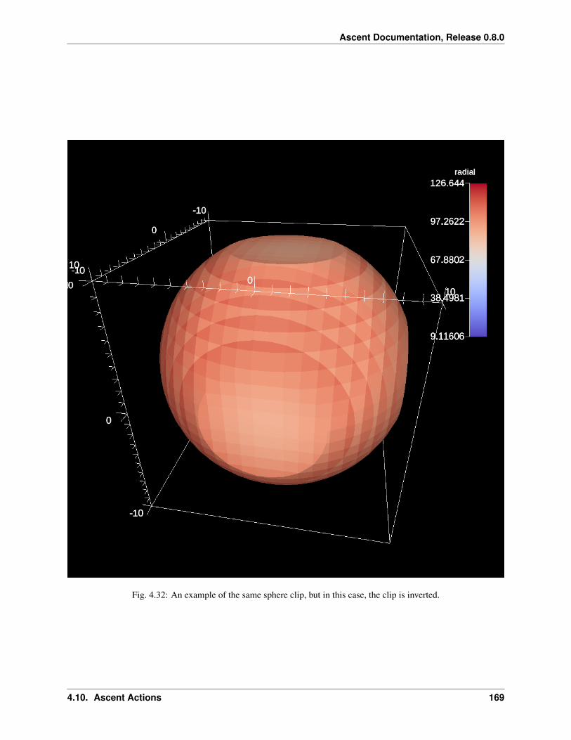
Ascent Documentation, Release 0.8.0
Fig. 4.32: An example of the same sphere clip, but in this case, the clip is inverted.
4.10. Ascent Actions 169

Ascent Documentation, Release 0.8.0
Fig. 4.33: A box clip of the same data set that removes the octant on the positive x, y, and z axes.
170 Chapter 4. Ascent Documentation

Ascent Documentation, Release 0.8.0
Fig. 4.34: Clipping by a plane defined by a point on the plane and the plane normal.
4.10. Ascent Actions 171

Ascent Documentation, Release 0.8.0
Figures 4.31, 4.32, 4.33, and 4.34 show an images produced from the clip filter. All of the clip examples are locatedin the file clip test.
Clip By Field
The clip by field filter removes cells from the specified topology using the values in a scalar field. By default, all valuesbelow the clip value are removed from the data set. As with clip by implicit function, the clip can be inverted.
conduit::Node pipelines;// pipeline 1pipelines["pl1/f1/type"] = "clip_with_field";// filter knobsconduit::Node &clip_params = pipelines["pl1/f1/params"];clip_params["field"] = "braid";clip_params["clip_value"] = 0.;
conduit::Node pipelines;// pipeline 1pipelines["pl1/f1/type"] = "clip_with_field";// filter knobsconduit::Node &clip_params = pipelines["pl1/f1/params"];clip_params["field"] = "braid";clip_params["invert"] = "true";clip_params["clip_value"] = 0.;
IsoVolume
IsoVolume is a filter that clips a data set based on a minimum and maximum value in a scalar field. All value outsideof the minimum and maximum values are removed from the data set.
conduit::Node pipelines;// pipeline 1pipelines["pl1/f1/type"] = "iso_volume";// filter knobsconduit::Node &clip_params = pipelines["pl1/f1/params"];clip_params["field"] = "braid";clip_params["min_value"] = 5.;clip_params["max_value"] = 10.;
Vector Magnitude
Vector magnitude creates a new field on the data set representing the magitude of a vector variable. The only parame-ters are the input vector field name and the name of the new field.
conduit::Node pipelines;// pipeline 1pipelines["pl1/f1/type"] = "vector_magnitude";// filter knobs (all these are optional)conduit::Node ¶ms = pipelines["pl1/f1/params"];params["field"] = "vel"; // name of the vector fieldparams["output_name"] = "mag"; // name of the output field
172 Chapter 4. Ascent Documentation

Ascent Documentation, Release 0.8.0
Fig. 4.35: An example of clipping all values below 0 in a data set.
4.10. Ascent Actions 173

Ascent Documentation, Release 0.8.0
Fig. 4.36: An example of clipping all values above 0 in a data set.
174 Chapter 4. Ascent Documentation

Ascent Documentation, Release 0.8.0
Fig. 4.37: An example of creating a iso-volume of values between 5.0 and 10.0.
4.10. Ascent Actions 175

Ascent Documentation, Release 0.8.0
Fig. 4.38: An example of creating a pseudocolor plot of vector magnitude
176 Chapter 4. Ascent Documentation

Ascent Documentation, Release 0.8.0
Vector Component
Vector component creates a new scalar field on the data set by extracting a component of a vector field. There are threerequired parameters: the input field, the output field name, and the index of the component to extract.
conduit::Node pipelines;// pipeline 1pipelines["pl1/f1/type"] = "vector_component";// filter knobs (all these are optional)conduit::Node ¶ms = pipelines["pl1/f1/params"];params["field"] = "vel"; // name of the vector fieldparams["output_name"] = "vel_x"; // name of the output fieldparams["component"] = 0; // index of the component
Composite Vector
Composite Vector creates a new vector field on the data set by combining two or three scalar fields into a vector. Thefirst two fields are required and the presense of the third field dictates whether a 2D or 3D vector is created. Inputfields can be different types (e.g., int32 and float32), and the resulting vector field will be a float64.
conduit::Node pipelines;// pipeline 1pipelines["pl1/f1/type"] = "vector_component";// filter knobs (all these are optional)conduit::Node ¶ms = pipelines["pl1/f1/params"];params["field1"] = "pressure"; // (required)params["field1"] = "temperature"; // (required)params["field1"] = "bananas"; // (optional, 2D vector if not present)params["output_name"] = "my_vec"; // (required) name of the output fieldparams["component"] = 0; // (required) index of the component
Recenter
Recenter changes the association of a field. Fields associated with either element or vertex can be interchanged byaveraging the surrounding values. When recentering to a element associated field, all vertex values incident to aelement are averaged, and similarly when rencentering to a vertex associated field, all element values incident to thevertex are averaged. If a field is already of the desired associated, then the nothing is done and the field is simplypassed through the filter. Note: ghost zones must be available when the data set has more than one domain. Withoutghost, the averaging will not be smooth across domain boundaries.
conduit::Node pipelines;// pipeline 1pipelines["pl1/f1/type"] = "recenter";conduit::Node ¶ms = pipelines["pl1/f1/params"];params["field"] = "braid"; // name of the vector fieldparams["association"] = "vertex"; // output field association// or params["association"] = "element"; // output field association
Gradient
Computes the gradient of a vertex-centered input field for every element in the input data set. Fields will be automati-call recentered if they are elemenet-centered. The gradient computation can either generate cell center based gradients,
4.10. Ascent Actions 177

Ascent Documentation, Release 0.8.0
which are fast but less accurate, or more accurate but slower point based gradients (default).
conduit::Node pipelines;// pipeline 1pipelines["pl1/f1/type"] = "gradient";// filter knobs (all these are optional)conduit::Node ¶ms = pipelines["pl1/f1/params"];params["field"] = "velocity"; // (required)params["output_name"] = "my_grad"; // (required) name of the output fieldparams["use_cell_gradient"] = "false"; // (optional)
Vorticity
Computes the vorticity of a vertex-centered input field for every element in the input data set. Fields will be automati-call recentered if they are elemenet-centered. The vorticity computation (based on the gradient) can either generate cellcenter based gradients, which are fast but less accurate, or more accurate but slower point based gradients (default).
conduit::Node pipelines;// pipeline 1pipelines["pl1/f1/type"] = "vorticity";// filter knobs (all these are optional)conduit::Node ¶ms = pipelines["pl1/f1/params"];params["field"] = "velocity"; // (required)params["output_name"] = "my_vorticity";// (required) name of the output fieldparams["use_cell_gradient"] = "false"; // (optional)
Q-Criterion
Computes the qcriterion of a vertex-centered input field for every element in the input data set. Fields will be automat-icall recentered if they are elemenet-centered. The qcriterion computation (based on the gradient) can either generatecell center based gradients, which are fast but less accurate, or more accurate but slower point based gradients (default).
conduit::Node pipelines;// pipeline 1pipelines["pl1/f1/type"] = "qcriterion";// filter knobs (all these are optional)conduit::Node ¶ms = pipelines["pl1/f1/params"];params["field"] = "velocity"; // (required)params["output_name"] = "my_q"; // (required) name of the output fieldparams["use_cell_gradient"] = "false"; // (optional)
Partitioning
Partitioning meshes is commonly needed in order to evenly distribute work among many simulation ranks. Ascentutilizes the partition() functions provided from Conduit::Blueprint. Blueprint provides two partition()functions that can be used to split or recombine Blueprint meshes in serial or parallel. Full M:N repartioning issupported. The partition() functions are in the serial and parallel Blueprint libraries, respectively.
// Serialvoid conduit::blueprint::mesh::partition(const Node &mesh,
const Node &options,Node &output);
(continues on next page)
178 Chapter 4. Ascent Documentation

Ascent Documentation, Release 0.8.0
(continued from previous page)
// Parallelvoid conduit::blueprint::mpi::mesh::partition(const Node &mesh,
const Node &options,Node &output,MPI_Comm comm);
Partitioning meshes using Blueprint will use any options present to determine how the partitioning process will behave.Typically, a caller would pass options containing selections if pieces of domains are desired. The partitioner processesany selections and then examines the desired target number of domains and will then decide whether domains mustbe moved among ranks (only in parallel version) and then locally combined to achieve the target number of domains.The combining process will attempt to preserve the input topology type for the output topology. However, in caseswhere lower topologies cannot be used, the algorithm will promote the extracted domain parts towards more generaltopologies and use the one most appropriate to contain the inputs.
In parallel, the partition() function will make an effort to redistribute data across MPI ranks to attempt to balancehow data are assigned. Domains produced from selections are assigned round-robin across ranks from rank 0 throughrank N-1 until all domains have been assigned. This assignment is carried out after extracting selections locally sothey can be restributed among ranks before being combined into the target number of domains.
Options
The partition() functions accept a node containing options. The options node can be empty and all options areoptional. If no options are given, each input mesh domain will be fully selected. It is more useful to pass selectionsas part of the option node with additional options that tell the algorithm how to split or combine the inputs. If noselections are present in the options node then the partitioner will create selections of an appropriate type that selectsall elements in each input domain.
The target option is useful for setting the target number of domains in the final output mesh. If the target valueis larger than the number of input domains or selections then the mesh will be split to achieve that target number ofdomains. This may require further subdividing selections. Alternatively, if the target is smaller than the number ofselections then the selections will be combined to yield the target number of domains. The combining is done suchthat smaller element count domains are combined first. Additionally, Ascent provides an optional boolean parameter,distributed, which dictates if the number of chosen target domains is applied across ranks (true, default), or toeach rank individually (false).
Option Description Exampleselections A list of selection objects
that identify regions of inter-est from the input domains.Selections can be differenton each MPI rank.
selections:-type: logicalstart: [0,0,0]end: [9,9,9]domain_id: 10
If not given,the output will contain the number of selections. In parallel,the largest target value from the ranks will beused for all ranks.target: 4
4.10. Ascent Actions 179

Ascent Documentation, Release 0.8.0
Actions/examples/partition.png
Fig. 4.39: Partition used to re-partition a 7 domain mesh (left) to different target numbers of domains and to isolatelogical subsets.
180 Chapter 4. Ascent Documentation

Ascent Documentation, Release 0.8.0
fields An list of strings that indicate the names of the fields to extract in the output. If this option is not provided,allfields will be extracted.fields: ["dist", "pressure"]
mapping An integer that determines whether fields containing original domains and ids will be added in the output.These fields enable one to know where each vertex and element came from originally. Mapping is on by default. Anon-zero value turns it on and a zero value turns it off.mapping: 0
merge_tolerance A double value that indicates the max allowable distance between 2 points before they are consideredto be separate. 2 points spaced smaller than this distance will be merged when explicit coordsets are combined.
merge_tolerance: 0.000001
distributed An optional boolean value for parallel execution. If true,the chosen number of target domains will beapplied across all ranks. If false,the chosen number of target domains will be applied to each rank individually.
If not given,the default is true.
distributed: "false"
Selections
Selections can be specified in the options for the partition() function to select regions of interest that will par-ticipate in mesh partitioning. If selections are not used then all elements from the input meshes will be selected topartitipate in the partitioning process. Selections can be further subdivided if needed to arrive at the target number ofdomains. Selections can target specific domains and topologies as well. If a selection does not apply to the input meshdomains then no geometry is produced in the output for that selection.
The partition() function’s options support 4 types of selections:
SelectionType
Topologies Description
logical uniform,rectilinear,structuredIdentifies start and end logical IJK ranges to select sub-bricks of uniform, rectilinear, orstructured topologies. This selection is not compatible with other topologies.
explicit all Identifies an explicit list of element ids and it works with all topologies.ranges all Identifies ranges of element ids, provided as pairs so the user can select multiple contiguous
blocks of elements. This selection works with all topologiesfield all Uses a specified field to indicate destination domain for each element.
By default, a selection does not apply to any specific domain_id. A list of selections applied to a single input meshwill extract multiple new domains from that original input mesh. Since meshes are composed of many domains inpractice, selections can also be associated with certain domain_id values. Selections that provide a domain_id valuewill only match domains that either have a matching state/domain_id value or match its index in the input node’s listof children (if state/domain_id is not present).
Selections can apply to certain topology names as well. By default, the first topology is used but if the topologyname is provided then the selection will operate on the specified topology only.
4.10. Ascent Actions 181

Ascent Documentation, Release 0.8.0
Option Description Exampletype The selection type
selections:-type: logical
domain_id The domain_id to which the selec-tion will apply. This is almost al-ways an unsigned integer value.For field selections, domain_id is al-lowed to be a string “any” so a sin-gle selection can apply to many do-mains.
selections:-type: logicaldomain_id: 10
selections:-type: logicaldomain_id: any
topology The topology to which the selectionwill apply. selections:
-type: logicaldomain_id: 10topology: mesh
Logical Selection
The logical selection allows the partitioner to extract a logical IJK subset from uniform, rectilinear, or structuredtopologies. The selection is given as IJK start and end values. If the end values extend beyond the actual mesh’slogical extents, they will be clipped. The partitioner may automatically subdivide logical selections into smallerlogical selections, if needed, preserving the logical structure of the input topology into the output.
selections:-type: logicalstart: [0,0,0]end: [9,9,9]
Explicit Selection
The explicit selection allows the partitioner to extract a list of elements. This is used when the user wants to target aspecific set of elements. The output will result in an explicit topology.
selections:-type: explicitelements: [0,1,2,3,100,101,102]
Ranges Selection
The ranges selection is similar to the explicit selection except that it identifies ranges of elements using pairs ofnumbers. The list of ranges must be a multiple of 2 in length. The output will result in an explicit topology.
182 Chapter 4. Ascent Documentation

Ascent Documentation, Release 0.8.0
selections:-type: rangesranges: [0,3,100,102]
Field Selection
The field selection enables the partitioner to use partitions done by other tools using a field on the mesh as the sourceof the final domain number for each element. The field must be associated with the mesh elements. When using a fieldselection, the partitioner will make a best attempt to use the domain numbers to extract mesh pieces and reassemblethem into domains with those numberings. If a larger target value is specified, then field selections can sometimes bepartitioned further as explicit partitions. The field selection is unique in that its domain_id value can be set to “any”if it is desired that the field selection will be applied to all domains in the input mesh. The domain_id value can stillbe set to specific integer values to limit the set of domains over which the selection will be applied.
selections:-type: fielddomain_id: anyfield: fieldname
4.10.3 Scenes
A scene encapsulates the information required to generate one or more images. To define a scene, the user specifiesa collection of plots (e.g., volume or surface rendering) and associated parameters such as camera definitions, lightpositions, and annotations. The simplest plot description requires only a plot type and scalar field name. A scenedefined in this way uses the default data source, which is all of the data published by the simulation, and defaultsettings for camera position, image resolution, lighting, and annotations.
Default Images
When creating a scene, Ascent will set up camera and color table defualts. The only requirement is that either aimage_name or image_prefix be provided. Minimally, a scene consists of one plot and a parameter to specifythe output file name. Default images images have a resolution of 1024x1024.
conduit::Node scenes;scenes["s1/plots/p1/type"] = "pseudocolor";scenes["s1/plots/p1/field"] = "braid";// scene default image prefixscenes["s1/image_prefix"] = output_file_name;
If anything other than the default camera, annotation, image resolution, or color table parameters are needed, then arender will need to be specified. Renders are covered later in this section.
Image Prefix
The image_prefix is a string denotes a prefix to be used when saving the image. For multiple cycles, the cyclenumber will be appended to the image filename. Numeric formatting, similar to printf is supported within theimage prefix. Assuming the cycle is 10, here are some examples:
• image_: image_10.png
4.10. Ascent Actions 183

Ascent Documentation, Release 0.8.0
• image_%04d: image_0010.png
Image Name
The image_name parameter speficies the excact file name of the of the output image, and Ascent will append the.png to the image file name. If not changed, the image file will be overwritten.
Plots
We current have support for three plot types: pseudocolor, volume, and mesh. Both plots support node centered andelement centered scalar fields. Plots optionally consume the result of a pipeline, but if none is specified, then the plotinput is the published mesh data. Each scene can contain one or more plots. The plot interface is simply:
{"type" : "plot_name","pipeline" : "pipeline_name","field" : "field_name"
}
In c++, the equivalent declarations would be as follows:
conduit::Node plot;plot["type"] = "plot_name";plot["pipeline"] = "pipeline_name";plot["field"] = "field_name";
Pseudocolor
A pseudocolor plot simply renders the mesh coloring by the provided scalar field. Below is an example of creating ascene with a single pseudocolor plot with the default pipeline:
conduit::Node scenes;scenes["s1/plots/p1/type"] = "pseudocolor";scenes["s1/plots/p1/field"] = "braid";// scene default image prefixscenes["s1/image_prefix"] = output_file_name;
conduit::Node actions;conduit::Node &add_plots = actions.append();add_plots["action"] = "add_scenes";add_plots["scenes"] = scenes;
An example of creating a scene with a user defined pipeline:
conduit::Node pipelines;// pipeline 1pipelines["pl1/f1/type"] = "contour";// filter knobsconduit::Node &contour_params = pipelines["pl1/f1/params"];contour_params["field"] = "braid";contour_params["iso_values"] = 0.;
conduit::Node scenes;
(continues on next page)
184 Chapter 4. Ascent Documentation

Ascent Documentation, Release 0.8.0
(continued from previous page)
scenes["s1/plots/p1/type"] = "pseudocolor";scenes["s1/plots/p1/field"] = "radial";scenes["s1/plots/p1/pipeline"] = "pl1";scenes["s1/image_prefix"] = output_file;
conduit::Node actions;// add the pipelineconduit::Node &add_pipelines= actions.append();add_pipelines["action"] = "add_pipelines";add_pipelines["pipelines"] = pipelines;// add the scenesconduit::Node &add_scenes= actions.append();add_scenes["action"] = "add_scenes";add_scenes["scenes"] = scenes;
In addition to surfaces, this pseudocolor color plot can render point meshes with no additional parameters. While thereis a default point radius, the plot options allow for constant or variable radii.
conduit::Node scenes;scenes["s1/plots/p1/type"] = "pseudocolor";scenes["s1/plots/p1/field"] = "braid";scenes["s1/plots/p1/points/radius"] = 1.f;
For variable radii, the field values are used to scale each points radius relative to the global min and max scalar value.The inputs are the base radius size, and the delta (multiplier) of the radius. In the example below, scalar values at theminimum of the scalar range will have a radius of 0.25 and scalar values at the max will have radii of 0.25 + 0.5.
conduit::Node scenes;scenes["s1/plots/p1/type"] = "pseudocolor";scenes["s1/plots/p1/field"] = "braid";scenes["s1/plots/p1/points/radius"] = 0.25f;// this detla is relative to the base radiusscenes["s1/plots/p1/points/radius_delta"] = 2.0f;
Volume Plot
The volume plot produces a volume rendering of the provided scalar field. The code below creates a volume plot ofthe default pipeline.
conduit::Node scenes;scenes["s1/plots/p1/type"] = "volume";scenes["s1/plots/p1/field"] = "braid";
conduit::Node actions;conduit::Node &add_plots = actions.append();add_plots["action"] = "add_scenes";add_plots["scenes"] = scenes;
Mesh Plot
The mesh plot, displays the computational mesh over which the simulations variables are defined. The mesh plot isoften added to the scene window when other plots are visualized to allow individual cells to be clearly seen. The codebelow creates a volume plot of the default pipeline.
4.10. Ascent Actions 185

Ascent Documentation, Release 0.8.0
Fig. 4.40: Default heuristic for points size
186 Chapter 4. Ascent Documentation

Ascent Documentation, Release 0.8.0
Fig. 4.41: Point mesh rendered with a constant radius
4.10. Ascent Actions 187

Ascent Documentation, Release 0.8.0
Fig. 4.42: Point mesh rendered with a variable radius
188 Chapter 4. Ascent Documentation

Ascent Documentation, Release 0.8.0
conduit::Node scenes;scenes["s1/plots/p1/type"] = "mesh";
conduit::Node actions;conduit::Node &add_plots = actions.append();add_plots["action"] = "add_scenes";add_plots["scenes"] = scenes;
Fig. 4.43: A mesh plot of simple grid.
4.10. Ascent Actions 189

Ascent Documentation, Release 0.8.0
Color Tables
The color map translates normalized scalars to color values. Color maps can be applied to each each plot in a scene.Image of the color tables provided by VTK-m can be found in VTK-m Color Tables. Minimally, a color table nameneeds to be specified, but the color_table node allows you to specify RGB and Alpha (opacity) control pointsfor complete customization of color maps. Alpha control points are used when rendering volumes. The built-inColor map names are: Cool to Warm, Black-Body Radiation, Samsel Fire, Inferno, Linear YGB,Cold and Hot, Rainbow Desaturated, Cool to Warm (Extended), X Ray, Black, Blue andWhite, Viridis, Linear Green, Jet, and Rainbow. Colors are three double precision values between 0 and1. Alphas and positions are a single double precision values between 0 and 1.
Here is an example of specifying a color table by name:
conduit::Node scenes;scenes["s1/plots/p1/type"] = "pseudocolor";scenes["s1/plots/p1/field"] = "braid";scenes["s1/plots/p1/color_table/name"] = "Viridis";
Color in the table can be reversed through an optional parameter:
scenes["s1/plots/p1/color_table/reverse"] = "true";
Volume plots are special since ray casting blends colors together. When no color table is specified, alpha values areautomatically created, but when a color table is specified, then the color table needs to include alpha values. Otherwise,the volume plot will look exactly the same as a pseudocolor plot.
Here is an example of adding a custom color table to the volume plot:
conduit::Node control_points;conduit::Node &point1 = control_points.append();point1["type"] = "rgb";point1["position"] = 0.;double color[3] = {1., 0., 0.};point1["color"].set_float64_ptr(color, 3);
conduit::Node &point2 = control_points.append();point2["type"] = "rgb";point2["position"] = 0.5;color[0] = 0;color[1] = 1.;point2["color"].set_float64_ptr(color, 3);
conduit::Node &point3 = control_points.append();point3["type"] = "rgb";point3["position"] = 1.0;color[1] = 0;color[2] = 1.;point3["color"].set_float64_ptr(color, 3);
conduit::Node &point4 = control_points.append();point4["type"] = "alpha";point4["position"] = 0.;point4["alpha"] = 0.;
conduit::Node &point5 = control_points.append();point5["type"] = "alpha";point5["position"] = 1.0;
(continues on next page)
190 Chapter 4. Ascent Documentation

Ascent Documentation, Release 0.8.0
(continued from previous page)
point5["alpha"] = 1.;
conduit::Node scenes;scenes["s1/plots/p1/type"] = "volume";scenes["s1/plots/p1/field"] = "braid";scenes["s1/plots/p1/color_table/control_points"] = control_points;
conduit::Node actions;conduit::Node &add_plots = actions.append();add_plots["action"] = "add_scenes";add_plots["scenes"] = scenes;
Clamping Scalar Values
The minimum and maximum values of a scalar field varies with each simulation time step, and rendering plots of thesame field from different time steps causes inconsistent mappings from scalars values to colors. To create a consistentmapping, a plot has two optional parameters that clamp the scalar values to a given range. Any scalar value above themaximum value will be clamped to the maximum, and any scalar value below the minimum value will be clamped tothe minimum.
Here is an example of clamping the scalar values to the range [-0.5, 0.5].
conduit::Node scenes;scenes["s1/plots/p1/type"] = "pseudocolor";scenes["s1/plots/p1/field"] = "braid";scenes["s1/plots/p1/min_value"] = -0.5;scenes["s1/plots/p1/max_value"] = 0.5;
Renders (Optional)
Scenes contains a list of Renders that specify the parameters of a single image. If no render is specified, a defaultrender is created automatically. Here is an example of creating a scene with render with some basic parameters:
conduit::Node scenes;scenes["s1/plots/p1/type"] = "pseudocolor";scenes["s1/plots/p1/field"] = "braid";scenes["s1/image_prefix"] = output_file;
scenes["s1/renders/r1/image_width"] = 512;scenes["s1/renders/r1/image_height"] = 512;scenes["s1/renders/r1/image_name"] = output_file;
Now we add a second render to the same example using every available parameter:
scenes["s1/renders/r2/image_width"] = 300;scenes["s1/renders/r2/image_height"] = 400;scenes["s1/renders/r2/image_name"] = output_file2;double vec3[3];vec3[0] = 1.; vec3[1] = 1.; vec3[2] = 1.;scenes["s1/renders/r2/camera/look_at"].set_float64_ptr(vec3,3);vec3[0] = 15.; vec3[1] = 17.; vec3[2] = 15.;scenes["s1/renders/r2/camera/position"].set_float64_ptr(vec3,3);vec3[0] = 0.; vec3[1] = -1.; vec3[2] = 0.;
(continues on next page)
4.10. Ascent Actions 191

Ascent Documentation, Release 0.8.0
(continued from previous page)
scenes["s1/renders/r2/camera/up"].set_float64_ptr(vec3,3);scenes["s1/renders/r2/camera/fov"] = 45.;scenes["s1/renders/r2/camera/xpan"] = 1.;scenes["s1/renders/r2/camera/ypan"] = 1.;scenes["s1/renders/r2/camera/azimuth"] = 10.0;scenes["s1/renders/r2/camera/elevation"] = -10.0;scenes["s1/renders/r2/camera/zoom"] = 3.2;scenes["s1/renders/r2/camera/near_plane"] = 0.1;scenes["s1/renders/r2/camera/far_plane"] = 33.1;
{"renders":{
"r1":{"image_width": 300,"image_height": 400,"image_name": "some_image","camera":{
"look_at": [1.0, 1.0, 1.0],"position": [0.0, 25.0, 15.0],"up": [0.0, -1.0, 0.0],"fov": 60.0,"xpan": 0.0,"ypan": 0.0,"elevation": 10.0,"azimuth": -10.0,"zoom": 0.0,"near_plane": 0.1,"far_plane": 100.1
}}
}}
Additional Render Options
In addition to image and camera parameters, renders have several options that allow the users to control the appearanceof images. Below is a list of additional parameters:
• bg_color : an array of three floating point values that controls the background color.
• fg_color : an array of three floating point values that controls the foreground color. The foreground color isused to color annotations and mesh plot lines.
• annotations : controls if annotations are rendered or not. Valid values are "true" and "false".
• render_bg : controls if the background is rendered or not. If no background is rendered, the background willappear transparent. Valid values are "true" and "false".
• dataset_bounds : controls the dimensions of the rendered bounding box around the dataset. This willoverwrite the default bounding box based on the dataset’s dimensions. A valid value is an array of six doubles([xMin,xMax,yMin,yMax,zMin,zMax]) that define dimensions larger than the default.
192 Chapter 4. Ascent Documentation

Ascent Documentation, Release 0.8.0
Cinema Databases
The Cinema specification is a image-based solution for post-hoc exploration of simulation data. The idea behindCinema is images take many orders of magnitude less disk space than that of the entire simulation data. By savingimages instead of the full mesh, we can save data much more frequently, giving users access to more temporal fidelitythan would be possible otherwise. For a complete overview, see the SC 14 paper. Other Cinema resources can befound at Cinema Science.
Ascent currently supports the creation of the Astaire specification (spec A) which captures images of the scene frompositions on a spherical camera. The number of images are captured in the parameters phi and theta. phi specifiesthe number of divisions along the polar angle and theta specifies the number of divisions along the azimuth. Forexample, if phi = 4 and theta = 8 then the resulting database will contain 4 * 8 images per time step. TheCinema database can then be explored in a supported viewer. In the future we hope to integrate a web-based viewer toenable exploration of the Cinema database as the simulation is running.
conduit::Node scenes;scenes["scene1/plots/plt1/type"] = "pseudocolor";scenes["scene1/plots/plt1/params/field"] = "braid";// setup required cinema paramsscenes["scene1/renders/r1/type"] = "cinema";scenes["scene1/renders/r1/phi"] = 2;scenes["scene1/renders/r1/theta"] = 2;scenes["scene1/renders/r1/db_name"] = "example_db";
A full code example can be found in the test suite’s Cinema test.
4.10.4 Extracts
Extracts are an abstraction that enables the user to specify how they want to capture their data. In terms of Ascent,data capture sends data outside the Ascent infrastructure. Examples include writing out the raw simulation data to thefile system, creating HDF5 files, or sending the data off node (e.g., ADIOS).
Currently supported extracts include:
• Python : use a python script with NumPy to analyze mesh data
• Relay : leverages Conduit’s Relay library to do parallel I/O
• HTG : write a VTK HTG (HyperTreeGrid) file
• ADIOS : use ADIOS to send data to a separate resource
Python
Python extracts can execute arbitrary python code. Python code uses Conduit’s python interface to interrogate andretrieve mesh data. Code is executed on each MPI rank, and mpi4py can be used for collective communication.
conduit::Node extracts;extracts["e1/type"] = "python";extracts["e1/params/source"] = py_script;
Python source code is loaded into Ascent via a string that could be loaded from the file system
import numpy as npfrom mpi4py import MPI
(continues on next page)
4.10. Ascent Actions 193

Ascent Documentation, Release 0.8.0
(continued from previous page)
# obtain a mpi4py mpi comm objectcomm = MPI.Comm.f2py(ascent_mpi_comm_id())
# get this MPI task's published blueprint datamesh_data = ascent_data().child(0)
# fetch the numpy array for the energy field valuese_vals = mesh_data["fields/energy/values"]
# find the data extents of the energy field using mpi
# first get local extentse_min, e_max = e_vals.min(), e_vals.max()
# declare vars for reduce resultse_min_all = np.zeros(1)e_max_all = np.zeros(1)
# reduce to get global extentscomm.Allreduce(e_min, e_min_all, op=MPI.MIN)comm.Allreduce(e_max, e_max_all, op=MPI.MAX)
# compute bins on global extentsbins = np.linspace(e_min_all, e_max_all)
# get histogram counts for local datahist, bin_edges = np.histogram(e_vals, bins = bins)
# declare var for reduce resultshist_all = np.zeros_like(hist)
# sum histogram counts with MPI to get final histogramcomm.Allreduce(hist, hist_all, op=MPI.SUM)
The example above shows how a python script could be used to create a distributed-memory histogram of a meshvariable that has been published by a simulation.
import conduitimport ascent.mpi# we treat everything as a multi_domain in ascent so grab child 0n_mesh = ascent_data().child(0)ascent_opts = conduit.Node()ascent_opts['mpi_comm'].set(ascent_mpi_comm_id())a = ascent.mpi.Ascent()a.open(ascent_opts)a.publish(n_mesh)actions = conduit.Node()scenes = conduit.Node()scenes['s1/plots/p1/type'] = 'pseudocolor'scenes['s1/plots/p1/params/field'] = 'radial_vert'scenes['s1/image_prefix'] = 'tout_python_mpi_extract_inception'add_act =actions.append()add_act['action'] = 'add_scenes'add_act['scenes'] = scenesactions.append()['action'] = 'execute'a.execute(actions)a.close()
194 Chapter 4. Ascent Documentation

Ascent Documentation, Release 0.8.0
In addition to performing custom python analysis, your can create new data sets and plot them through a new instanceof Ascent. We call this technique Inception.
Relay
Relay extracts save data to the file system. Currently, Relay supports saving data to Blueprint HDF5, YAML, or JSONfiles. By default, Relay saves the published mesh data to the file system, but if a pipeline is specified, then the resultof the pipeline is saved. Relay extracts can be opened by post-hoc tools such as VisIt.
conduit::Node pipelines;// pipeline 1pipelines["pl1/f1/type"] = "contour";// filter knobsconduit::Node &contour_params = pipelines["pl1/f1/params"];contour_params["field"] = "radial_vert";contour_params["iso_values"] = 250.;
conduit::Node extracts;extracts["e1/type"] = "relay";extracts["e1/pipeline"] = "pl1";
extracts["e1/params/path"] = output_file;
In this example, a contour of a field is saved to the file system in json form. To save the files in HDF5 format:
extracts["e1/params/protocol"] = "hdf5";
yaml and json are also valid protocol options.
By default, the relay extract creates one file per mesh domain saved. You can control the number of files written(aggregating multiple domains per file) using the num_files parameter:
extracts["e1/params/num_files"] = 2;
Additionally, Relay supports saving out only a subset of the data. The fields parameters is a list of strings thatindicate which fields should be saved.
extracts["e1/params/fields"].append("density");extracts["e1/params/fields"].append("pressure");
HTG
HTG extracts save data to the file system as a VTK HyperTreeGrid. HyperTreeGrid is a tree based uniform gridfor element based data. The current implementation writes out binary trees from uniform grids. As such there are anumber of limitations on the type of data it writes out. These include the following:
• The mesh must be a uniform grid.
• The mesh must have a pwer of 2 number of elements in each direction.
• The mesh dimensions must be the same in each direction.
• The fields must be element based.
The extract also takes a blank_value parameter that specifies a field value that indicates that the cell is empty.
4.10. Ascent Actions 195

Ascent Documentation, Release 0.8.0
conduit::Node data;conduit::blueprint::mesh::examples::basic("uniform", 33, 33, 33, data);
conduit::Node extracts;extracts["e1/type"] = "htg";
extracts["e1/params/path"] = "basic_mesh33x33x33";extracts["e1/params/blank_value"] = -10000.;
conduit::Node actions;// add the extractsconduit::Node &add_extracts = actions.append();add_extracts["action"] = "add_extracts";add_extracts["extracts"] = extracts;
conduit::Node &execute = actions.append();execute["action"] = "execute";
//// Run Ascent//Ascent ascent;
Node ascent_opts;ascent_opts["runtime"] = "ascent";ascent.open(ascent_opts);ascent.publish(data);ascent.execute(actions);ascent.close();
In this example, the field is saved to the file system in basic_mesh33x33x33.htg.
Additionally, HTG supports saving out only a subset of the data. The fields parameters is a list of strings that indicatewhich fields should be saved.
extracts["e1/params/fields"].append("density");extracts["e1/params/fields"].append("pressure");
Flatten
Flatten extracts save data to the file system. Currently, Flatten supports saving data to Blueprint HDF5, YAML, CSV(default), or JSON files. By default, Flatten saves the published mesh data to the file system, but if a pipeline isspecified, then the result of the pipeline is saved. Flatten transforms the data from Blueprint Meshes to BlueprintTables. This extract generates two files: one for vertex data and one for element data.
This extract requires a path for the location of the resulting files. Optional parameters include protocol for thetype of output file (default is CSV), and fields, which specifies the fields to be included in the files (default is allpresent fields).
ADIOS
The current ADIOS extract is experimental and this section is under construction.
196 Chapter 4. Ascent Documentation

Ascent Documentation, Release 0.8.0
4.10.5 ParaView Visualization
The section ParaView Support describes how to install Ascent with ParaView support and how to run the exampleintegrations using insitu ParaView pipelines. In this section we describe in detail the ParaView visualization pipelinefor cloverleaf3d, one of the example integrations, and we provide implementation details for the Ascent ParaViewintegration.
The ParaView pipeline for cloverleaf3d
First we need to tell Ascent that we are using a Python script to visualize data using ascent-actions.json.
[{"action": "add_extracts","extracts":{
"e1":{
"type": "python","params":{
"file": "paraview-vis.py"}
}}
}]
The ParaView pipeline for the cloverleaf3d sample integration is in paraview-vis.py.
We use a variable count to be able to distinguish timestep 0, when we setup the visualization pipeline. For alltimesteps including timestep 0, we execute the visualization pipeline we setup at timestep 0.
try:count = count + 1
except NameError:count = 0
For timestep 0, we initialize ParaView,
if count == 0:import paraviewparaview.options.batch = Trueparaview.options.symmetric = True
then we load the AscentSource plugin and we create the object that presents the simulation data as a VTK dataset.We also create a view of the same size as the image we want to save.
#LoadPlugin("@PARAVIEW_ASCENT_SOURCE@", remote=True, ns=globals())ascentSource = AscentSource()view = CreateRenderView()view.ViewSize = [1024, 1024]
From the VTK dataset, we select only the cells that are not ghosts and show them colored by the energy scalar. Notethat for a ParaView filter that has no input specified, the output data from the previous command in the program isused. So SelectCells uses the output data from ascentSource.
4.10. Ascent Actions 197

Ascent Documentation, Release 0.8.0
#sel = SelectCells("vtkGhostType < 1")e = ExtractSelection(Selection=sel)rep = Show()ColorBy(rep, ("CELLS", "energy"))
We rescale the transfer function, show a scalar bar, and change the viewing direction
#transferFunction = GetColorTransferFunction('energy')transferFunction.RescaleTransferFunction(1, 5.5)renderView1 = GetActiveView()scalarBar = GetScalarBar(transferFunction, renderView1)scalarBar.Title = 'energy'scalarBar.ComponentTitle = ''scalarBar.Visibility = 1rep.SetScalarBarVisibility(renderView1, True)cam = GetActiveCamera()cam.Elevation(30)cam.Azimuth(-30)
For all timesteps, UpdateAscentData sets the new Ascent data and marks the VTK source as modi-fied. This insures that a new VTK dataset will be computed when we need to Render. We also callUpdatePropertyInformation which insures that property values are available to the script. There are twoproperties setup on AscentSource: Time (this represents the simulation time and is the same as state/timein Conduit Blueprint Mesh specification) and Cycle (this represents the simulation time step when the visualiza-tion pipeline is called and is the same as state/cycle in Conduit Blueprint Mesh specification). After that, weResetCamera so that the image fits the screen properly, we render and save the image to a file.
ascentSource.UpdateAscentData()ascentSource.UpdatePropertyInformation()cycle = GetProperty(ascentSource, "Cycle").GetElement(0)imageName = "image_{0:04d}.png".format(int(cycle))ResetCamera()Render()SaveScreenshot(imageName, ImageResolution=(1024, 1024))
This script saves an image for each cycle with the image for cycle 200 shown next.
Implementation details
The Ascent ParaView integration is implemented in the src/examples/paraview-vis directory in the Ascent distribution.
AscentSource class, found in paraview_ascent_source.py, derives fromVTKPythonAlgorithmBase and produces one of the following datasets: vtkImageData,vtkRectilinearGrid, vtkStructuredGrid or vtkUnstructuredGrid. AscentSource re-ceives from an instrumented simulation a tree structure (json like) that describes the simulation data using the ConduitBlueprint Mesh specification. This data is converted to a VTK format using zero copy for data arrays.
Global extents are not passed for the existing example integrations so they are computed (using MPI communication)for uniform and rectilinear topologies but they are not computed for a structured topology (lulesh integration exam-ple). This means that for lulesh and datasets that have a structured topology we cannot save a correct parallel filethat represents the whole dataset, unless the global extents are passed from the simulation.
A ParaView pipeline for each sample simulation is specified in a paraview-vis-XXX.py file where XXX is thename of the simulation. In this file, we load the ParaView plugin and setup the pipeline for timestep 0 and update thepipeline and save a screenshot for each timestep of the simulation.
198 Chapter 4. Ascent Documentation

Ascent Documentation, Release 0.8.0
Fig. 4.44: CloverLeaf3D visualized with a ParaView pipeline
4.10. Ascent Actions 199

Ascent Documentation, Release 0.8.0
4.10.6 Triggers
Triggers allow the user to specify a set of actions that are triggered by the result of a boolean expression. Triggersleverage the query and expression system to enable a set of primitives to create custom tailored triggers for simula-tions. There are several motivations that make triggers useful. Examples include cost reduction (time) and debugging(correctness).
Cost Reduction
Visualization and analysis operation are not free, i.e., performing them takes time. One example is that rendering animage every simulation cycle might be a relatively high cost. Another example is performing a potentially time con-suming operation like flow field analysis may might need to take place at a lower frequency than each time ascent.execute(actions) is called or may need to execute only when a specific simulation event occurs.
Debugging
Triggers can be a useful tool in detecting anomalous conditions while a simulation is running. For example, triggerscan detect of the minimum or maximum values of a field are outside the expected ranges and dump out the mesh andrelated field for inspection inside of VisIt.
Simple Example
A trigger requires a trigger condition and a actions file:
-action: "add_triggers"triggers:t1:
params:condition: "cycle() % 100 == 0"actions_file : "my_trigger_actions.yaml"
In this example, the trigger will fire when the current cycle is divisible by 100.
Queries and Triggers
Triggers can leverage the query system, and combining both queries and triggers creates a rich set of potential optionsfor triggers.
Debugging
The following code example shows how queries and triggers can be used for debugging:
-action: "add_queries"queries:q1:
params:# get the maximum value of a fieldexpression: "max(field('pressure'))"name: "max_pressure"
(continues on next page)
200 Chapter 4. Ascent Documentation

Ascent Documentation, Release 0.8.0
(continued from previous page)
q2:params:
expression: "1e300"name: "crazy_value"
-action: "add_triggers"triggers:t1:
params:condition: "max_pressure > crazy_value"actions_file : "my_trigger_actions.yaml"
In the above example, the trigger will fire if the maximum value of pressure exceeds crazy_value. A useful actionsfile might dump the mesh to a hdf5 file for later inspection.
Event Detection
The following code example shows how queries and triggers can be used for to detect a jump in entropy that couldrepresent a simulation event that the user wants act on:
-action: "add_queries"queries:q1:
params:expression: "entropy(histogram(field('pressure')))"name: "entropy"
-action: "add_triggers"triggers:t1:
params:condition: "history(entropy, relative_index = 1) - entropy > 10"actions_file : "my_trigger_actions.yaml"
In the above example, the trigger will fire if the change in entropy changes by more than 10 in positive direction.
4.10.7 Ascent Actions Examples
An example of the contour filter with a single iso value.
YAML actions:
#An example of the contour filter with a single iso value.
-action: "add_pipelines"pipelines:pl1:
f1:type: "contour"params:field: "braid"
(continues on next page)
4.10. Ascent Actions 201

Ascent Documentation, Release 0.8.0
(continued from previous page)
iso_values: 0.0-
action: "add_scenes"scenes:s1:
plots:p1:type: "pseudocolor"field: "radial"pipeline: "pl1"
image_prefix: "/Users/harrison37/Work/alpine/ascent/build-debug/tests/_output/→˓tout_single_contour_3d"
Resulting image:
202 Chapter 4. Ascent Documentation

Ascent Documentation, Release 0.8.0
An example of rendering a point field with constant radius.
YAML actions:
#An example of rendering a point field with constant radius.
-action: "add_scenes"scenes:s1:
plots:p1:type: "pseudocolor"field: "braid"points:
radius: 1.0image_prefix: "/Users/harrison37/Work/alpine/ascent/build-debug/tests/_output/
→˓tout_render_3d_points_const_radius"
Resulting image:
4.10. Ascent Actions 203

Ascent Documentation, Release 0.8.0
An example of rendering with no screen annotations.
YAML actions:
#An example of rendering with no screen annotations.
-action: "add_scenes"scenes:s1:
plots:p1:type: "pseudocolor"
(continues on next page)
204 Chapter 4. Ascent Documentation

Ascent Documentation, Release 0.8.0
(continued from previous page)
field: "braid"renders:
r1:image_prefix: "/Users/harrison37/Work/alpine/ascent/build-debug/tests/_
→˓output/tout_render_3d_no_screen_annotations"screen_annotations: "false"
Resulting image:
An example of creating a mesh plot.
YAML actions:
4.10. Ascent Actions 205

Ascent Documentation, Release 0.8.0
#An example of creating a mesh plot.
-action: "add_scenes"scenes:s1:
plots:p1:type: "mesh"
image_prefix: "/Users/harrison37/Work/alpine/ascent/build-debug/tests/_output/→˓tout_render_3d_mesh"
Resulting image:
206 Chapter 4. Ascent Documentation

Ascent Documentation, Release 0.8.0
An example of using the volume (unstructured grid) extract.
YAML actions:
#An example of using the volume (unstructured grid) extract.
-action: "add_extracts"extracts:e1:
type: "volume"params:
field: "radial"filename: "/Users/larsen30/research/test_builds/devil_ray/ascent/build/tests/_
→˓output/tout_rover_volume"
Resulting image:
4.10. Ascent Actions 207

Ascent Documentation, Release 0.8.0
An example of using the log2 filter and clamping the min value. This can help when there arenegative values present.
YAML actions:
#An example of using the log2 filter and clamping the min value. This can help when→˓there are negative values present.
-action: "add_pipelines"pipelines:pl1:
f1:
(continues on next page)
208 Chapter 4. Ascent Documentation

Ascent Documentation, Release 0.8.0
(continued from previous page)
type: "vector_magnitude"params:field: "vel"output_name: "mag"
f2:type: "log2"params:field: "mag"output_name: "log2_mag"clamp_min_value: 2.0
-action: "add_scenes"scenes:s1:
plots:p1:type: "pseudocolor"field: "log2_mag"pipeline: "pl1"
image_prefix: "/Users/harrison37/Work/alpine/ascent/build-debug/tests/_output/→˓tout_log2_field_clamp"
Resulting image:
4.10. Ascent Actions 209

Ascent Documentation, Release 0.8.0
An example if using the vector component filter to extract a scalar component of a vector field.
YAML actions:
#An example if using the vector component filter to extract a scalar component of a→˓vector field.
-action: "add_pipelines"pipelines:pl1:
f1:type: "vector_component"
(continues on next page)
210 Chapter 4. Ascent Documentation

Ascent Documentation, Release 0.8.0
(continued from previous page)
params:field: "vel"component: 0output_name: "my_vec_comp"
-action: "add_scenes"scenes:s1:
plots:p1:type: "pseudocolor"field: "my_vec_comp"pipeline: "pl1"
image_prefix: "/Users/harrison37/Work/alpine/ascent/build-debug/tests/_output/→˓tout_vector_component"
Resulting image:
4.10. Ascent Actions 211

Ascent Documentation, Release 0.8.0
An example of rendering with no world annotations.
YAML actions:
#An example of rendering with no world annotations.
-action: "add_scenes"scenes:s1:
plots:p1:type: "pseudocolor"
(continues on next page)
212 Chapter 4. Ascent Documentation

Ascent Documentation, Release 0.8.0
(continued from previous page)
field: "braid"renders:
r1:image_prefix: "/Users/harrison37/Work/alpine/ascent/build-debug/tests/_
→˓output/tout_render_3d_no_world_annotations"world_annotations: "false"
Resulting image:
An example of using the log filter.
YAML actions:
4.10. Ascent Actions 213

Ascent Documentation, Release 0.8.0
#An example of using the log filter.
-action: "add_pipelines"pipelines:pl1:
f1:type: "scale"params:x_scale: 2.0y_scale: 2.0z_scale: 2.0
-action: "add_scenes"scenes:s1:
plots:p1:type: "pseudocolor"field: "braid"pipeline: "pl1"
image_prefix: "/Users/harrison37/Work/alpine/ascent/build-debug/tests/_output/→˓tout_scale"
Resulting image:
214 Chapter 4. Ascent Documentation

Ascent Documentation, Release 0.8.0
An example of creating a render, specifying all camera parameters.
YAML actions:
#An example of creating a render, specifying all camera parameters.
-action: "add_scenes"scenes:s1:
plots:p1:type: "volume"
(continues on next page)
4.10. Ascent Actions 215

Ascent Documentation, Release 0.8.0
(continued from previous page)
field: "braid"color_table:
name: "blue"control_points:-type: "rgb"position: 0.0color: [1.0, 0.0, 0.0]
-type: "rgb"position: 0.5color: [0.0, 1.0, 0.0]
-type: "rgb"position: 1.0color: [1.0, 1.0, 1.0]
-type: "alpha"position: 0.0alpha: 0.0
-type: "alpha"position: 1.0alpha: 1.0
image_prefix: "/Users/harrison37/Work/alpine/ascent/build-debug/tests/_output/→˓render_0"
renders:r1:image_width: 512image_height: 512image_prefix: "/Users/harrison37/Work/alpine/ascent/build-debug/tests/_
→˓output/render_0"r2:image_width: 400image_height: 400image_prefix: "/Users/harrison37/Work/alpine/ascent/build-debug/tests/_
→˓output/render_1"camera:look_at: [1.0, 1.0, 1.0]position: [0.0, 25.0, 15.0]up: [0.0, -1.0, 0.0]fov: 60.0xpan: 0.0ypan: 0.0zoom: 1.0azimuth: 10.0elevation: -10.0near_plane: 0.1far_plane: 100.1
Resulting image:
216 Chapter 4. Ascent Documentation

Ascent Documentation, Release 0.8.0
An example rendering a 2d field.
YAML actions:
#An example rendering a 2d field.
-action: "add_scenes"scenes:scene1:
plots:plt1:type: "pseudocolor"
(continues on next page)
4.10. Ascent Actions 217

Ascent Documentation, Release 0.8.0
(continued from previous page)
field: "braid"image_prefix: "/Users/harrison37/Work/alpine/ascent/build-debug/tests/_output/
→˓tout_render_2d_default_runtime"
Resulting image:
An example of using the log filter.
YAML actions:
#An example of using the log filter.
(continues on next page)
218 Chapter 4. Ascent Documentation

Ascent Documentation, Release 0.8.0
(continued from previous page)
-action: "add_pipelines"pipelines:pl1:
f1:type: "vector_magnitude"params:field: "vel"output_name: "mag"
f2:type: "log"params:field: "mag"output_name: "log_mag"
-action: "add_scenes"scenes:s1:
plots:p1:type: "pseudocolor"field: "log_mag"pipeline: "pl1"
image_prefix: "/Users/harrison37/Work/alpine/ascent/build-debug/tests/_output/→˓tout_log_field"
Resulting image:
4.10. Ascent Actions 219

Ascent Documentation, Release 0.8.0
An example of rendering with no background (alpha channel = 0)
YAML actions:
#An example of rendering with no background (alpha channel = 0)
-action: "add_scenes"scenes:s1:
plots:p1:type: "pseudocolor"
(continues on next page)
220 Chapter 4. Ascent Documentation

Ascent Documentation, Release 0.8.0
(continued from previous page)
field: "braid"renders:
r1:image_prefix: "/Users/harrison37/Work/alpine/ascent/build-debug/tests/_
→˓output/tout_render_3d_no_bg"render_bg: "false"
Resulting image:
An example of changing the azimuth of the camera.
YAML actions:
4.10. Ascent Actions 221

Ascent Documentation, Release 0.8.0
#An example of changing the azimuth of the camera.
-action: "add_scenes"scenes:s1:
plots:p1:type: "pseudocolor"field: "braid"
renders:r1:camera:azimuth: 1.0
image_prefix: "/Users/harrison37/Work/alpine/ascent/build-debug/tests/_→˓output/tout_render_3d_azimuth"
Resulting image:
222 Chapter 4. Ascent Documentation

Ascent Documentation, Release 0.8.0
An example of the contour filter with a number of evenly spaced levels.
YAML actions:
#An example of the contour filter with a number of evenly spaced levels.
-action: "add_pipelines"pipelines:pl1:
f1:type: "contour"params:
(continues on next page)
4.10. Ascent Actions 223

Ascent Documentation, Release 0.8.0
(continued from previous page)
field: "braid"levels: 5
-action: "add_scenes"scenes:s1:
plots:p1:type: "pseudocolor"field: "radial"pipeline: "pl1"
image_prefix: "/Users/harrison37/Work/alpine/ascent/build-debug/tests/_output/→˓tout_multi_contour_levels"
Resulting image:
224 Chapter 4. Ascent Documentation

Ascent Documentation, Release 0.8.0
An example changing the rendering bounds of a 3d field.
YAML actions:
#An example changing the rendering bounds of a 3d field.
-action: "add_scenes"scenes:scene1:
plots:plt1:type: "pseudocolor"
(continues on next page)
4.10. Ascent Actions 225

Ascent Documentation, Release 0.8.0
(continued from previous page)
field: "braid"renders:
r1:camera:azimuth: 30
image_prefix: "/Users/harrison37/Work/alpine/ascent/build-debug/tests/_→˓output/tout_render_bounds_3d"
dataset_bounds: [-15.0, 15.0, -15.0, 15.0, -15.0, 15.0]
Resulting image:
226 Chapter 4. Ascent Documentation

Ascent Documentation, Release 0.8.0
An example changing the rendering bounds of a 2d field.
YAML actions:
#An example changing the rendering bounds of a 2d field.
-action: "add_scenes"scenes:scene1:
plots:plt1:type: "pseudocolor"field: "braid"
renders:r1:image_prefix: "/Users/harrison37/Work/alpine/ascent/build-debug/tests/_
→˓output/tout_render_bounds_2d"dataset_bounds: [-15.0, 15.0, -15.0, 15.0, 0.0, 0.0]
Resulting image:
4.10. Ascent Actions 227

Ascent Documentation, Release 0.8.0
An example of the sampling filter using histogram-based approach.
YAML actions:
#An example of the sampling filter using histogram-based approach.
-action: "add_pipelines"pipelines:pl1:
f1:type: "histsampling"params:
(continues on next page)
228 Chapter 4. Ascent Documentation

Ascent Documentation, Release 0.8.0
(continued from previous page)
field: "braid"sample_rate: 0.1bins: 32
-action: "add_scenes"scenes:s1:
plots:p1:type: "pseudocolor"field: "radial"pipeline: "pl1"
image_prefix: "/Users/harrison37/Work/alpine/ascent/build-debug/tests/_output/→˓tout_sampling_3d"
Resulting image:
4.10. Ascent Actions 229

Ascent Documentation, Release 0.8.0
An example an inverted sphere clip using a center and radius
YAML actions:
#An example an inverted sphere clip using a center and radius
-action: "add_pipelines"pipelines:pl1:
f1:type: "clip"params:
(continues on next page)
230 Chapter 4. Ascent Documentation

Ascent Documentation, Release 0.8.0
(continued from previous page)
invert: "true"sphere:
radius: 11.0center:x: 0.0y: 0.0z: 0.0
-action: "add_scenes"scenes:s1:
plots:p1:type: "pseudocolor"field: "radial"pipeline: "pl1"
image_prefix: "/Users/harrison37/Work/alpine/ascent/build-debug/tests/_output/→˓tout_clip_inverted_sphere"
Resulting image:
4.10. Ascent Actions 231

Ascent Documentation, Release 0.8.0
An example of creating a transfer function for volume rendering.
YAML actions:
#An example of creating a transfer function for volume rendering.
-action: "add_pipelines"pipelines:pl1:
f1:type: "contour"params:
(continues on next page)
232 Chapter 4. Ascent Documentation

Ascent Documentation, Release 0.8.0
(continued from previous page)
field: "braid"iso_values: 0.0
-action: "add_scenes"scenes:s1:
plots:p1:type: "pseudocolor"field: "radial"pipeline: "pl1"
p2:type: "volume"field: "braid"min_value: -0.5max_value: 0.5color_table:
name: "rainbow desaturated"control_points:-type: "alpha"position: 0.0alpha: 0.0
-type: "alpha"position: 1.0alpha: 0.5
image_prefix: "/Users/harrison37/Work/alpine/ascent/build-debug/tests/_output/→˓tout_render_3d_multi_default_runtime"
Resulting image:
4.10. Ascent Actions 233

Ascent Documentation, Release 0.8.0
An example of specifying trigger actions without a trigger trigger actions file.
YAML actions:
#An example of specifying trigger actions without a trigger trigger actions file.
-action: "add_triggers"triggers:t1:
params:condition: "magnitude(max(field('braid')).position - vector(0,0,0)) > 0"actions:
(continues on next page)
234 Chapter 4. Ascent Documentation
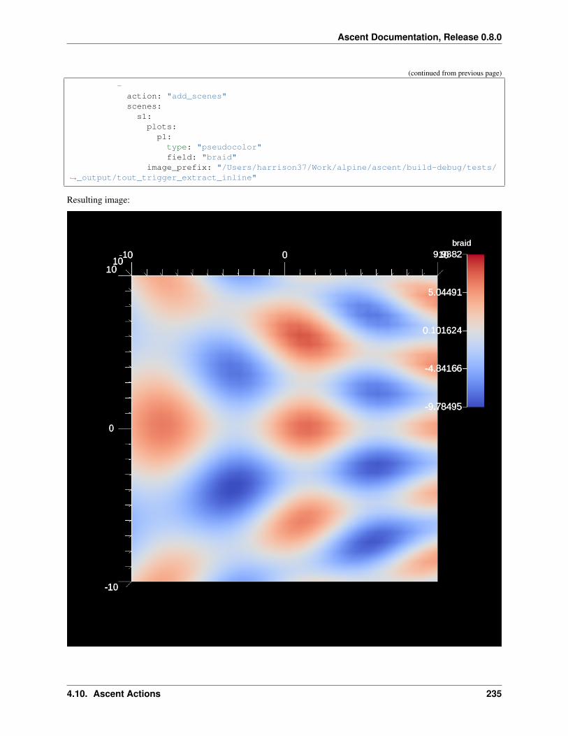
Ascent Documentation, Release 0.8.0
(continued from previous page)
-action: "add_scenes"scenes:s1:plots:p1:type: "pseudocolor"field: "braid"
image_prefix: "/Users/harrison37/Work/alpine/ascent/build-debug/tests/→˓_output/tout_trigger_extract_inline"
Resulting image:
4.10. Ascent Actions 235

Ascent Documentation, Release 0.8.0
An example of the interconnecting pipelines.
YAML actions:
#An example of the interconnecting pipelines.
-action: "add_pipelines"pipelines:pl1:
f1:type: "vector_magnitude"params:field: "vel"output_name: "mag"
pl2:pipeline: "pl1"f1:
type: "log"params:field: "mag"output_name: "log_mag"
-action: "add_scenes"scenes:s1:
plots:p1:type: "pseudocolor"field: "log_mag"pipeline: "pl2"
image_prefix: "/Users/harrison37/Work/alpine/ascent/build-debug/tests/_output/→˓tout_pipelines"
Resulting image:
236 Chapter 4. Ascent Documentation

Ascent Documentation, Release 0.8.0
•
YAML actions:
-action: "add_pipelines"pipelines:pl1:
f1:type: "contour"params:field: "e"levels: 5
f2:type: "log2"
(continues on next page)
4.10. Ascent Actions 237

Ascent Documentation, Release 0.8.0
(continued from previous page)
params:field: "e"output_name: "log2_energy"clamp_min_value: 1.0
-action: "add_scenes"scenes:s1:
plots:p1:type: "pseudocolor"field: "log2_energy"pipeline: "pl1"
renders:r1:image_prefix: "contour_log2_energy_%04d"camera:azimuth: 135
Resulting image:
238 Chapter 4. Ascent Documentation

Ascent Documentation, Release 0.8.0
An example of using the gradient filter and plotting the magnitude.
YAML actions:
#An example of using the gradient filter and plotting the magnitude.
-action: "add_pipelines"pipelines:pl1:
f2:type: "vorticity"params:
(continues on next page)
4.10. Ascent Actions 239

Ascent Documentation, Release 0.8.0
(continued from previous page)
field: "vel"output_name: "vel_vorticity"use_cell_gradient: "false"
f1:type: "vector_magnitude"params:field: "vel_vorticity"output_name: "mag_vorticity"
-action: "add_scenes"scenes:s1:
plots:p1:type: "pseudocolor"field: "mag_vorticity"pipeline: "pl1"
image_prefix: "/Users/harrison37/Work/alpine/ascent/build-debug/tests/_output/→˓tout_vorticity_vel"
Resulting image:
240 Chapter 4. Ascent Documentation

Ascent Documentation, Release 0.8.0
An example of the three slice filter.
YAML actions:
#An example of the three slice filter.
-action: "add_pipelines"pipelines:pl1:
f1:type: "3slice"params:
(continues on next page)
4.10. Ascent Actions 241

Ascent Documentation, Release 0.8.0
(continued from previous page)
x_offset: 1.0y_offset: 0.0z_offset: -1.0
-action: "add_scenes"scenes:s1:
plots:p1:type: "pseudocolor"field: "radial"pipeline: "pl1"
image_prefix: "/Users/harrison37/Work/alpine/ascent/build-debug/tests/_output/→˓tout_3slice_3d"
Resulting image:
242 Chapter 4. Ascent Documentation

Ascent Documentation, Release 0.8.0
An example of disabling a color table.
YAML actions:
#An example of disabling a color table.
-action: "add_scenes"scenes:s1:
plots:p1:type: "pseudocolor"
(continues on next page)
4.10. Ascent Actions 243

Ascent Documentation, Release 0.8.0
(continued from previous page)
field: "braid"color_table:
annotation: "false"image_prefix: "/Users/harrison37/Work/alpine/ascent/build-debug/tests/_output/
→˓no_color_bar"renders:
r1:image_width: 512image_height: 512image_prefix: "/Users/harrison37/Work/alpine/ascent/build-debug/tests/_
→˓output/no_color_bar"
Resulting image:
244 Chapter 4. Ascent Documentation

Ascent Documentation, Release 0.8.0
An example of using the volume (unstructured grid) extract with min and max values.
YAML actions:
#An example of using the volume (unstructured grid) extract with min and max values.
-action: "add_extracts"extracts:e1:
type: "volume"params:
field: "radial"min_value: -1.0emission: "radial"precision: "double"filename: "/Users/larsen30/research/test_builds/devil_ray/ascent/build/tests/_
→˓output/tout_rover_volume_min_max"
Resulting image:
4.10. Ascent Actions 245

Ascent Documentation, Release 0.8.0
An example of filtering fields not present in the actions file.
YAML actions:
#An example of filtering fields not present in the actions file.
-action: "add_scenes"scenes:s1:
plots:p1:type: "pseudocolor"
(continues on next page)
246 Chapter 4. Ascent Documentation
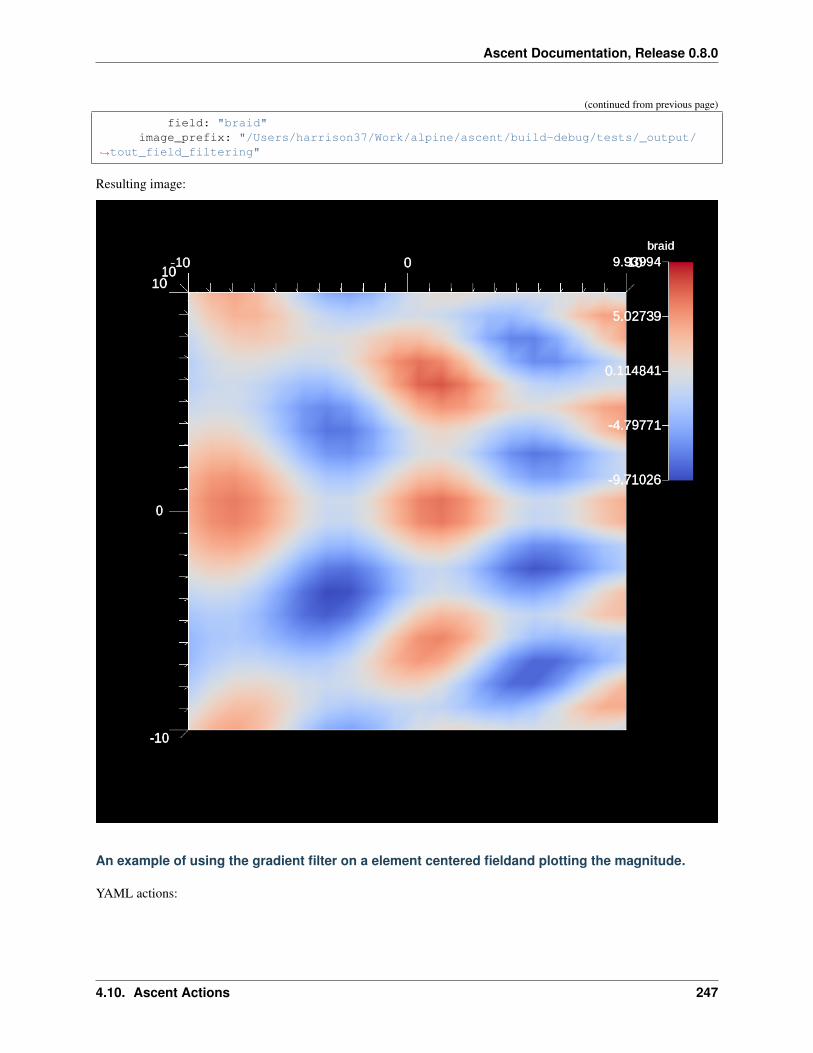
Ascent Documentation, Release 0.8.0
(continued from previous page)
field: "braid"image_prefix: "/Users/harrison37/Work/alpine/ascent/build-debug/tests/_output/
→˓tout_field_filtering"
Resulting image:
An example of using the gradient filter on a element centered fieldand plotting the magnitude.
YAML actions:
4.10. Ascent Actions 247

Ascent Documentation, Release 0.8.0
#An example of using the gradient filter on a element centered fieldand plotting the→˓magnitude.
-action: "add_pipelines"pipelines:pl1:
f2:type: "gradient"params:field: "radial"output_name: "radial_gradient"
f1:type: "vector_magnitude"params:field: "radial_gradient"output_name: "mag_grad"
-action: "add_scenes"scenes:s1:
plots:p1:type: "pseudocolor"field: "mag_grad"pipeline: "pl1"
image_prefix: "/Users/harrison37/Work/alpine/ascent/build-debug/tests/_output/→˓tout_gradient_mag_radial"
Resulting image:
248 Chapter 4. Ascent Documentation

Ascent Documentation, Release 0.8.0
An example of the contour filter with a multiple iso values.
YAML actions:
#An example of the contour filter with a multiple iso values.
-action: "add_pipelines"pipelines:pl1:
f1:type: "contour"params:
(continues on next page)
4.10. Ascent Actions 249

Ascent Documentation, Release 0.8.0
(continued from previous page)
field: "braid"iso_values: [-0.4, 0.2, 0.4]
-action: "add_scenes"scenes:s1:
plots:p1:type: "pseudocolor"field: "radial"pipeline: "pl1"
image_prefix: "/Users/harrison37/Work/alpine/ascent/build-debug/tests/_output/→˓tout_multi_contour_3d"
Resulting image:
250 Chapter 4. Ascent Documentation

Ascent Documentation, Release 0.8.0
An example of the slice filter with a single plane.
YAML actions:
#An example of the slice filter with a single plane.
-action: "add_pipelines"pipelines:pl1:
f1:type: "slice"params:
(continues on next page)
4.10. Ascent Actions 251

Ascent Documentation, Release 0.8.0
(continued from previous page)
point:x: 0.0y: 0.0z: 0.0
normal:x: 0.0y: 0.0z: 1.0
-action: "add_scenes"scenes:s1:
plots:p1:type: "pseudocolor"field: "radial"pipeline: "pl1"
image_prefix: "/Users/harrison37/Work/alpine/ascent/build-debug/tests/_output/→˓tout_slice_3d"
Resulting image:
252 Chapter 4. Ascent Documentation

Ascent Documentation, Release 0.8.0
An example of creating a mesh plot of a contour.
YAML actions:
#An example of creating a mesh plot of a contour.
-action: "add_pipelines"pipelines:pl1:
f1:type: "contour"params:
(continues on next page)
4.10. Ascent Actions 253

Ascent Documentation, Release 0.8.0
(continued from previous page)
field: "braid"iso_values: 0.0
-action: "add_scenes"scenes:s1:
plots:p1:type: "pseudocolor"field: "radial"pipeline: "pl1"
p2:type: "mesh"pipeline: "pl1"
image_prefix: "/Users/harrison37/Work/alpine/ascent/build-debug/tests/_output/→˓tout_render_3d_multi_mesh"
Resulting image:
254 Chapter 4. Ascent Documentation

Ascent Documentation, Release 0.8.0
An example of using inverted clip with field.
YAML actions:
#An example of using inverted clip with field.
-action: "add_pipelines"pipelines:pl1:
f1:type: "clip_with_field"params:
(continues on next page)
4.10. Ascent Actions 255

Ascent Documentation, Release 0.8.0
(continued from previous page)
field: "braid"clip_value: 0.0invert: "true"
-action: "add_scenes"scenes:s1:
plots:p1:type: "pseudocolor"field: "radial"pipeline: "pl1"
image_prefix: "/Users/harrison37/Work/alpine/ascent/build-debug/tests/_output/→˓tout_clip_with_field_inverted"
Resulting image:
256 Chapter 4. Ascent Documentation

Ascent Documentation, Release 0.8.0
An example if using the vector magnitude filter.
YAML actions:
#An example if using the vector magnitude filter.
-action: "add_pipelines"pipelines:pl1:
f1:type: "vector_magnitude"params:
(continues on next page)
4.10. Ascent Actions 257

Ascent Documentation, Release 0.8.0
(continued from previous page)
field: "vel"output_name: "mag"
-action: "add_scenes"scenes:s1:
plots:p1:type: "pseudocolor"field: "mag"pipeline: "pl1"
image_prefix: "/Users/harrison37/Work/alpine/ascent/build-debug/tests/_output/→˓tout_vec_mag"
Resulting image:
258 Chapter 4. Ascent Documentation

Ascent Documentation, Release 0.8.0
An example of using the log filter and clamping the min value. This can help when there are negativevalues present.
YAML actions:
#An example of using the log filter and clamping the min value. This can help when→˓there are negative values present.
-action: "add_pipelines"pipelines:pl1:
f1:
(continues on next page)
4.10. Ascent Actions 259

Ascent Documentation, Release 0.8.0
(continued from previous page)
type: "vector_magnitude"params:field: "vel"output_name: "mag"
f2:type: "log"params:field: "mag"output_name: "log_mag"clamp_min_value: 2.0
-action: "add_scenes"scenes:s1:
plots:p1:type: "pseudocolor"field: "log_mag"pipeline: "pl1"
image_prefix: "/Users/harrison37/Work/alpine/ascent/build-debug/tests/_output/→˓tout_log_field_clamp"
Resulting image:
260 Chapter 4. Ascent Documentation

Ascent Documentation, Release 0.8.0
An example of the slice filter with a single plane (off-axis).
YAML actions:
#An example of the slice filter with a single plane (off-axis).
-action: "add_pipelines"pipelines:pl1:
f1:type: "slice"params:
(continues on next page)
4.10. Ascent Actions 261

Ascent Documentation, Release 0.8.0
(continued from previous page)
point:x: 1.0y: 1.0z: 1.0
normal:x: 0.0y: 0.0z: 1.0
-action: "add_scenes"scenes:s1:
plots:p1:type: "pseudocolor"field: "radial"pipeline: "pl1"
image_prefix: "/Users/harrison37/Work/alpine/ascent/build-debug/tests/_output/→˓tout_slice_3d_off_axis"
Resulting image:
262 Chapter 4. Ascent Documentation

Ascent Documentation, Release 0.8.0
An example of the slice filter with a single plane.
YAML actions:
#An example of the slice filter with a single plane.
-action: "add_pipelines"pipelines:pl1:
f1:type: "exaslice"params:
(continues on next page)
4.10. Ascent Actions 263

Ascent Documentation, Release 0.8.0
(continued from previous page)
point:x: 0.0y: 0.0z: 0.0
normal:x: 0.0y: 0.0z: 1.0
-action: "add_scenes"scenes:s1:
plots:p1:type: "pseudocolor"field: "radial"pipeline: "pl1"
image_prefix: "/Users/harrison37/Work/alpine/ascent/build-debug/tests/_output/→˓tout_exaslice_3d"
Resulting image:
264 Chapter 4. Ascent Documentation

Ascent Documentation, Release 0.8.0
An example of creating a plot specifying the min and max values of the scalar range.
YAML actions:
#An example of creating a plot specifying the min and max values of the scalar range.
-action: "add_scenes"scenes:s1:
plots:p1:type: "pseudocolor"
(continues on next page)
4.10. Ascent Actions 265

Ascent Documentation, Release 0.8.0
(continued from previous page)
field: "braid"min_value: -0.5max_value: 0.5
image_prefix: "/Users/harrison37/Work/alpine/ascent/build-debug/tests/_output/→˓tout_render_3d_ascent_min_max"
Resulting image:
An example a plane clip defined with a point and a normal
YAML actions:
266 Chapter 4. Ascent Documentation

Ascent Documentation, Release 0.8.0
#An example a plane clip defined with a point and a normal
-action: "add_pipelines"pipelines:pl1:
f1:type: "clip"params:plane:
point:x: 0.0y: 0.0z: 0.0
normal:x: 1.0y: 0.0z: 0
-action: "add_scenes"scenes:s1:
plots:p1:type: "pseudocolor"field: "radial"pipeline: "pl1"
image_prefix: "/Users/harrison37/Work/alpine/ascent/build-debug/tests/_output/→˓tout_clip_plane"
Resulting image:
4.10. Ascent Actions 267

Ascent Documentation, Release 0.8.0
An example of using clip with field.
YAML actions:
#An example of using clip with field.
-action: "add_pipelines"pipelines:pl1:
f1:type: "clip_with_field"params:
(continues on next page)
268 Chapter 4. Ascent Documentation

Ascent Documentation, Release 0.8.0
(continued from previous page)
field: "braid"clip_value: 0.0
-action: "add_scenes"scenes:s1:
plots:p1:type: "pseudocolor"field: "radial"pipeline: "pl1"
image_prefix: "/Users/harrison37/Work/alpine/ascent/build-debug/tests/_output/→˓tout_clip_with_field"
Resulting image:
4.10. Ascent Actions 269

Ascent Documentation, Release 0.8.0
An example if using the re-center filter (to vertex).
YAML actions:
#An example if using the re-center filter (to vertex).
-action: "add_pipelines"pipelines:pl1:
f1:type: "recenter"params:
(continues on next page)
270 Chapter 4. Ascent Documentation

Ascent Documentation, Release 0.8.0
(continued from previous page)
field: "radial"association: "vertex"
-action: "add_scenes"scenes:s1:
plots:p1:type: "pseudocolor"field: "radial"pipeline: "pl1"
image_prefix: "/Users/harrison37/Work/alpine/ascent/build-debug/tests/_output/→˓tout_recenter_element"
Resulting image:
4.10. Ascent Actions 271

Ascent Documentation, Release 0.8.0
An example of rendering with no annotations.
YAML actions:
#An example of rendering with no annotations.
-action: "add_scenes"scenes:s1:
plots:p1:type: "pseudocolor"
(continues on next page)
272 Chapter 4. Ascent Documentation

Ascent Documentation, Release 0.8.0
(continued from previous page)
field: "braid"renders:
r1:image_prefix: "/Users/harrison37/Work/alpine/ascent/build-debug/tests/_
→˓output/tout_render_3d_no_annotations"annotations: "false"
Resulting image:
An example of rendering custom background and foreground colors.
YAML actions:
4.10. Ascent Actions 273

Ascent Documentation, Release 0.8.0
#An example of rendering custom background and foreground colors.
-action: "add_scenes"scenes:s1:
plots:p1:type: "pseudocolor"field: "braid"
renders:r1:image_prefix: "/Users/harrison37/Work/alpine/ascent/build-debug/tests/_
→˓output/tout_render_3d_bg_fg_colors"bg_color: [1.0, 1.0, 1.0]fg_color: [0.0, 0.0, 0.0]
Resulting image:
274 Chapter 4. Ascent Documentation

Ascent Documentation, Release 0.8.0
An example of using the isovolume filter.
YAML actions:
#An example of using the isovolume filter.
-action: "add_pipelines"pipelines:pl1:
f1:type: "isovolume"params:
(continues on next page)
4.10. Ascent Actions 275

Ascent Documentation, Release 0.8.0
(continued from previous page)
field: "braid"min_value: 5.0max_value: 10.0
-action: "add_scenes"scenes:s1:
plots:p1:type: "pseudocolor"field: "radial"pipeline: "pl1"
image_prefix: "/Users/harrison37/Work/alpine/ascent/build-debug/tests/_output/→˓tout_iso_volume"
Resulting image:
276 Chapter 4. Ascent Documentation

Ascent Documentation, Release 0.8.0
An example if using the re-center filter (to element).
YAML actions:
#An example if using the re-center filter (to element).
-action: "add_pipelines"pipelines:pl1:
f1:type: "recenter"params:
(continues on next page)
4.10. Ascent Actions 277

Ascent Documentation, Release 0.8.0
(continued from previous page)
field: "braid"association: "element"
-action: "add_scenes"scenes:s1:
plots:p1:type: "pseudocolor"field: "braid"pipeline: "pl1"
image_prefix: "/Users/harrison37/Work/alpine/ascent/build-debug/tests/_output/→˓tout_recenter_vertex"
Resulting image:
278 Chapter 4. Ascent Documentation

Ascent Documentation, Release 0.8.0
An example of using the gradient filter and plotting the magnitude.
YAML actions:
#An example of using the gradient filter and plotting the magnitude.
-action: "add_pipelines"pipelines:pl1:
f2:type: "divergence"params:
(continues on next page)
4.10. Ascent Actions 279

Ascent Documentation, Release 0.8.0
(continued from previous page)
field: "vel"output_name: "vel_divergence"use_cell_gradient: "false"
-action: "add_scenes"scenes:s1:
plots:p1:type: "pseudocolor"field: "vel_divergence"pipeline: "pl1"
image_prefix: "/Users/harrison37/Work/alpine/ascent/build-debug/tests/_output/→˓tout_divergence_vel"
Resulting image:
280 Chapter 4. Ascent Documentation

Ascent Documentation, Release 0.8.0
An example of the slice filter with a single plane.
YAML actions:
#An example of the slice filter with a single plane.
-action: "add_pipelines"pipelines:pl1:
f1:type: "slice"params:
(continues on next page)
4.10. Ascent Actions 281

Ascent Documentation, Release 0.8.0
(continued from previous page)
point:x_offset: 0.0y_offset: -0.5z_offset: 0.0
normal:x: 1.0y: 1.0z: 1.0
-action: "add_scenes"scenes:s1:
plots:p1:type: "pseudocolor"field: "radial"pipeline: "pl1"
image_prefix: "/Users/harrison37/Work/alpine/ascent/build-debug/tests/_output/→˓tout_slice_offset_3d"
Resulting image:
282 Chapter 4. Ascent Documentation

Ascent Documentation, Release 0.8.0
An example of using the gradient filter and plotting the magnitude.
YAML actions:
#An example of using the gradient filter and plotting the magnitude.
-action: "add_pipelines"pipelines:pl1:
f2:type: "qcriterion"params:
(continues on next page)
4.10. Ascent Actions 283

Ascent Documentation, Release 0.8.0
(continued from previous page)
field: "vel"output_name: "vel_qcriterion"use_cell_gradient: "false"
-action: "add_scenes"scenes:s1:
plots:p1:type: "pseudocolor"field: "vel_qcriterion"pipeline: "pl1"
image_prefix: "/Users/harrison37/Work/alpine/ascent/build-debug/tests/_output/→˓tout_qcriterion_vel"
Resulting image:
284 Chapter 4. Ascent Documentation

Ascent Documentation, Release 0.8.0
Example of rendering multiple topologies
YAML actions:
#Example of rendering multiple topologies
-action: "add_scenes"scenes:s1:
plots:p1:type: "pseudocolor"
(continues on next page)
4.10. Ascent Actions 285

Ascent Documentation, Release 0.8.0
(continued from previous page)
field: "braid"color_table:
name: "Inferno"p2:type: "pseudocolor"field: "point_braid"points:radius: 0.5
renders:r1:image_prefix: "/Users/harrison37/Work/alpine/ascent/build-debug/tests/_
→˓output/tout_multi_topo"annotations: "false"camera:azimuth: 30elevation: 11
Resulting image:
286 Chapter 4. Ascent Documentation

Ascent Documentation, Release 0.8.0
An example of creating a render specifying the image size.
YAML actions:
#An example of creating a render specifying the image size.
-action: "add_scenes"scenes:s1:
plots:p1:type: "pseudocolor"
(continues on next page)
4.10. Ascent Actions 287

Ascent Documentation, Release 0.8.0
(continued from previous page)
field: "rank_ele"renders:
r1:image_width: 512image_height: 512image_prefix: "/Users/harrison37/Work/alpine/ascent/build-debug/tests/_
→˓output/tout_render_3d_domain_overload"camera:azimuth: 45.0
Resulting image:
288 Chapter 4. Ascent Documentation

Ascent Documentation, Release 0.8.0
An example a blox clip
YAML actions:
#An example a blox clip
-action: "add_pipelines"pipelines:pl1:
f1:type: "clip"params:box:
min:x: 0.0y: 0.0z: 0.0
max:x: 10.01y: 10.01z: 10.01
-action: "add_scenes"scenes:s1:
plots:p1:type: "pseudocolor"field: "radial"pipeline: "pl1"
image_prefix: "/Users/harrison37/Work/alpine/ascent/build-debug/tests/_output/→˓tout_clip_box"
Resulting image:
4.10. Ascent Actions 289

Ascent Documentation, Release 0.8.0
An example of using the log10 filter.
YAML actions:
#An example of using the log10 filter.
-action: "add_pipelines"pipelines:pl1:
f1:type: "vector_magnitude"params:
(continues on next page)
290 Chapter 4. Ascent Documentation

Ascent Documentation, Release 0.8.0
(continued from previous page)
field: "vel"output_name: "mag"
f2:type: "log10"params:field: "mag"output_name: "log10_mag"
-action: "add_scenes"scenes:s1:
plots:p1:type: "pseudocolor"field: "log10_mag"pipeline: "pl1"
image_prefix: "/Users/harrison37/Work/alpine/ascent/build-debug/tests/_output/→˓tout_log10_field"
Resulting image:
4.10. Ascent Actions 291

Ascent Documentation, Release 0.8.0
An example of using the log2 filter.
YAML actions:
#An example of using the log2 filter.
-action: "add_pipelines"pipelines:pl1:
f1:type: "vector_magnitude"params:
(continues on next page)
292 Chapter 4. Ascent Documentation

Ascent Documentation, Release 0.8.0
(continued from previous page)
field: "vel"output_name: "mag"
f2:type: "log2"params:field: "mag"output_name: "log2_mag"
-action: "add_scenes"scenes:s1:
plots:p1:type: "pseudocolor"field: "log2_mag"pipeline: "pl1"
image_prefix: "/Users/harrison37/Work/alpine/ascent/build-debug/tests/_output/→˓tout_log2_field"
Resulting image:
4.10. Ascent Actions 293

Ascent Documentation, Release 0.8.0
An example of creating a custom color map.
YAML actions:
#An example of creating a custom color map.
-action: "add_scenes"scenes:s1:
plots:p1:type: "pseudocolor"
(continues on next page)
294 Chapter 4. Ascent Documentation

Ascent Documentation, Release 0.8.0
(continued from previous page)
field: "braid"color_table:
control_points:-type: "rgb"position: 0.0color: [0.23, 0.08, 0.08]
-type: "rgb"position: 0.5color: [0.48, 0.23, 0.04]
-type: "rgb"position: 1.0color: [0.99, 1.0, 0.96]
image_prefix: "/Users/harrison37/Work/alpine/ascent/build-debug/tests/_output/→˓milk_chocolate"
renders:r1:image_width: 512image_height: 512image_prefix: "/Users/harrison37/Work/alpine/ascent/build-debug/tests/_
→˓output/milk_chocolate"
Resulting image:
4.10. Ascent Actions 295

Ascent Documentation, Release 0.8.0
An example if using the composite vector filter to compose three scalar fields into a vector.
YAML actions:
#An example if using the composite vector filter to compose three scalar fields into→˓a vector.
-action: "add_pipelines"pipelines:pl1:
f1:type: "composite_vector"
(continues on next page)
296 Chapter 4. Ascent Documentation

Ascent Documentation, Release 0.8.0
(continued from previous page)
params:field1: "braid"field2: "braid"field3: "braid"output_name: "my_vec"
f2:type: "vector_magnitude"params:field: "my_vec"output_name: "my_vec_mag"
-action: "add_scenes"scenes:s1:
plots:p1:type: "pseudocolor"field: "my_vec_mag"pipeline: "pl1"
image_prefix: "/Users/harrison37/Work/alpine/ascent/build-debug/tests/_output/→˓tout_composite_vector"
Resulting image:
4.10. Ascent Actions 297

Ascent Documentation, Release 0.8.0
An example a sphere clip using a center and radius
YAML actions:
#An example a sphere clip using a center and radius
-action: "add_pipelines"pipelines:pl1:
f1:type: "clip"params:
(continues on next page)
298 Chapter 4. Ascent Documentation

Ascent Documentation, Release 0.8.0
(continued from previous page)
sphere:radius: 11.0center:x: 0.0y: 0.0z: 0.0
-action: "add_scenes"scenes:s1:
plots:p1:type: "pseudocolor"field: "radial"pipeline: "pl1"
image_prefix: "/Users/harrison37/Work/alpine/ascent/build-debug/tests/_output/→˓tout_clip_sphere"
Resulting image:
4.10. Ascent Actions 299

Ascent Documentation, Release 0.8.0
Example of adding 1 ghost field with 2 topologies
YAML actions:
#Example of adding 1 ghost field with 2 topologies
-action: "add_scenes"scenes:s1:
plots:p1:type: "pseudocolor"
(continues on next page)
300 Chapter 4. Ascent Documentation

Ascent Documentation, Release 0.8.0
(continued from previous page)
field: "braid"p2:type: "pseudocolor"field: "point_braid"points:
radius: 0.5renders:
r1:image_prefix: "/Users/harrison37/Work/alpine/ascent/build-debug/tests/_
→˓output/tout_multi_topo_single_ghost"annotations: "false"camera:azimuth: 30elevation: 11
Resulting image:
4.10. Ascent Actions 301

Ascent Documentation, Release 0.8.0
An example of using the gradient filter and plotting the magnitude.
YAML actions:
#An example of using the gradient filter and plotting the magnitude.
-action: "add_pipelines"pipelines:pl1:
f2:type: "gradient"params:
(continues on next page)
302 Chapter 4. Ascent Documentation

Ascent Documentation, Release 0.8.0
(continued from previous page)
field: "braid"output_name: "braid_gradient"use_cell_gradient: "true"
f1:type: "vector_magnitude"params:field: "braid_gradient"output_name: "mag_grad"
-action: "add_scenes"scenes:s1:
plots:p1:type: "pseudocolor"field: "mag_grad"pipeline: "pl1"
image_prefix: "/Users/harrison37/Work/alpine/ascent/build-debug/tests/_output/→˓tout_cell_gradient_mag_braid"
Resulting image:
4.10. Ascent Actions 303

Ascent Documentation, Release 0.8.0
An example of using queries in filter parameters.
YAML actions:
#An example of using queries in filter parameters.
-action: "add_queries"queries:q1:
params:expression: "min(field('braid')).value"name: "min_value"
(continues on next page)
304 Chapter 4. Ascent Documentation

Ascent Documentation, Release 0.8.0
(continued from previous page)
q2:params:
expression: "max(field('braid')).value"name: "max_value"
q3:params:
expression: "max_value - min_value"name: "length"
-action: "add_pipelines"pipelines:pl1:
f1:type: "threshold"params:field: "braid"min_value: "0.75 * length + min_value"max_value: "max_value"
-action: "add_scenes"scenes:s1:
plots:p1:type: "pseudocolor"field: "braid"pipeline: "pl1"
image_prefix: "/Users/harrison37/Work/alpine/ascent/build-debug/tests/_output/→˓tout_filter_params_query"
Resulting image:
4.10. Ascent Actions 305

Ascent Documentation, Release 0.8.0
An example of rendering a point field with variable radius.
YAML actions:
#An example of rendering a point field with variable radius.
-action: "add_scenes"scenes:s1:
plots:p1:type: "pseudocolor"
(continues on next page)
306 Chapter 4. Ascent Documentation

Ascent Documentation, Release 0.8.0
(continued from previous page)
field: "braid"points:
radius: 0.25radius_delta: 2.0
image_prefix: "/Users/harrison37/Work/alpine/ascent/build-debug/tests/_output/→˓tout_render_3d_points_variable_radius"
Resulting image:
•
YAML actions:
4.10. Ascent Actions 307

Ascent Documentation, Release 0.8.0
-action: "add_pipelines"pipelines:pl1:
f1:type: "contour"params:field: "e"levels: 10
f2:type: "log10"params:field: "e"output_name: "log10_energy"clamp_min_value: 1.0
-action: "add_scenes"scenes:s1:
plots:p1:type: "pseudocolor"field: "log10_energy"pipeline: "pl1"
renders:r1:image_prefix: "contour_log10_energy_%04d"camera:azimuth: 135
Resulting image:
308 Chapter 4. Ascent Documentation

Ascent Documentation, Release 0.8.0
An example of using the threshold filter.
YAML actions:
#An example of using the threshold filter.
-action: "add_pipelines"pipelines:pl1:
f1:type: "threshold"params:
(continues on next page)
4.10. Ascent Actions 309

Ascent Documentation, Release 0.8.0
(continued from previous page)
field: "braid"min_value: -0.2max_value: 0.2
-action: "add_scenes"scenes:s1:
plots:p1:type: "pseudocolor"field: "braid"pipeline: "pl1"
image_prefix: "/Users/harrison37/Work/alpine/ascent/build-debug/tests/_output/→˓tout_threshold_3d"
Resulting image:
310 Chapter 4. Ascent Documentation

Ascent Documentation, Release 0.8.0
A more complex trigger example using several functions that evaluate positons on the mesh.
YAML actions:
#A more complex trigger example using several functions that evaluate positons on the→˓mesh.
-action: "add_triggers"triggers:t1:
params:condition: "magnitude(max(field('braid')).position - vector(0,0,0)) > 0"
(continues on next page)
4.10. Ascent Actions 311

Ascent Documentation, Release 0.8.0
(continued from previous page)
actions_file: "/Users/harrison37/Work/alpine/ascent/build-debug/tests/_output/→˓complex_trigger_actions"
Resulting image:
Example of adding multple ghosts with 2 topologies
YAML actions:
#Example of adding multple ghosts with 2 topologies
-
(continues on next page)
312 Chapter 4. Ascent Documentation

Ascent Documentation, Release 0.8.0
(continued from previous page)
action: "add_scenes"scenes:s1:
plots:p1:type: "pseudocolor"field: "braid"
p2:type: "pseudocolor"field: "point_braid"points:
radius: 0.5renders:
r1:image_prefix: "/Users/harrison37/Work/alpine/ascent/build-debug/tests/_
→˓output/tout_multi_topo_ghosts"annotations: "false"camera:azimuth: 30elevation: 11
Resulting image:
4.10. Ascent Actions 313

Ascent Documentation, Release 0.8.0
An example of using the gradient filter and plotting the magnitude.
YAML actions:
#An example of using the gradient filter and plotting the magnitude.
-action: "add_pipelines"pipelines:pl1:
f2:type: "gradient"params:
(continues on next page)
314 Chapter 4. Ascent Documentation

Ascent Documentation, Release 0.8.0
(continued from previous page)
field: "braid"output_name: "braid_gradient"
f1:type: "vector_magnitude"params:field: "braid_gradient"output_name: "mag_grad"
-action: "add_scenes"scenes:s1:
plots:p1:type: "pseudocolor"field: "mag_grad"pipeline: "pl1"
image_prefix: "/Users/harrison37/Work/alpine/ascent/build-debug/tests/_output/→˓tout_gradient_mag_braid"
Resulting image:
4.10. Ascent Actions 315

Ascent Documentation, Release 0.8.0
An example of using the log10 filter and clamping the min value. This can help when there arenegative values present.
YAML actions:
#An example of using the log10 filter and clamping the min value. This can help when→˓there are negative values present.
-action: "add_pipelines"pipelines:pl1:
f1:
(continues on next page)
316 Chapter 4. Ascent Documentation

Ascent Documentation, Release 0.8.0
(continued from previous page)
type: "vector_magnitude"params:field: "vel"output_name: "mag"
f2:type: "log10"params:field: "mag"output_name: "log10_mag"clamp_min_value: 2.0
-action: "add_scenes"scenes:s1:
plots:p1:type: "pseudocolor"field: "log10_mag"pipeline: "pl1"
image_prefix: "/Users/harrison37/Work/alpine/ascent/build-debug/tests/_output/→˓tout_log10_field_clamp"
Resulting image:
4.10. Ascent Actions 317

Ascent Documentation, Release 0.8.0
An example of using the gradient filter using cell gradients on a element centered field and plottingthe magnitude.
YAML actions:
#An example of using the gradient filter using cell gradients on a element centered→˓field and plotting the magnitude.
-action: "add_pipelines"pipelines:pl1:
f2:
(continues on next page)
318 Chapter 4. Ascent Documentation

Ascent Documentation, Release 0.8.0
(continued from previous page)
type: "gradient"params:field: "radial"output_name: "radial_gradient"use_cell_gradient: "true"
f1:type: "vector_magnitude"params:field: "radial_gradient"output_name: "mag_grad"
-action: "add_scenes"scenes:s1:
plots:p1:type: "pseudocolor"field: "mag_grad"pipeline: "pl1"
image_prefix: "/Users/harrison37/Work/alpine/ascent/build-debug/tests/_output/→˓tout_cell_gradient_mag_radial"
Resulting image:
4.10. Ascent Actions 319

Ascent Documentation, Release 0.8.0
An example of using the xray extract.
YAML actions:
#An example of using the xray extract.
-action: "add_extracts"extracts:e1:
type: "xray"params:
absorption: "radial"
(continues on next page)
320 Chapter 4. Ascent Documentation

Ascent Documentation, Release 0.8.0
(continued from previous page)
filename: "/Users/larsen30/research/test_builds/devil_ray/ascent/build/tests/_→˓output/tout_rover_xray_params"
image_params:min_value: 0.00600000005215406max_value: 1.0log_scale: "true"
unit_scalar: 0.00100000004749745
An example of using devil ray scalar rendering.
YAML actions:
#An example of using devil ray scalar rendering.
-action: "add_extracts"extracts:e1:
type: "relay"pipeline: "pl1"params:
path: "/Users/larsen30/research/test_builds/devil_ray/ascent/build/tests/_→˓output/tout_scalar_renderer"
protocol: "blueprint/mesh/hdf5"-
action: "add_pipelines"pipelines:pl1:
f1:type: "dray_project_2d"params:image_width: 512image_height: 512fields:
- "density"
An example of using a relay extract to save a subset of the data.
YAML actions:
#An example of using a relay extract to save a subset of the data.
-action: "add_extracts"extracts:e1:
type: "relay"params:
path: "/Users/harrison37/Work/alpine/ascent/build-debug/tests/_output/tout_→˓relay_serial_extract_subset"
protocol: "blueprint/mesh/hdf5"fields:- "braid"- "radial"
(continues on next page)
4.10. Ascent Actions 321

Ascent Documentation, Release 0.8.0
(continued from previous page)
-action: "execute"
A more complex trigger example using several functions that evaluate positons on the mesh.
YAML actions:
#A more complex trigger example using several functions that evaluate positons on the→˓mesh.
-action: "add_triggers"triggers:t1:
params:condition: "magnitude(max(field('braid')).position - vector(0,0,0)) > 0"actions_file: "/Users/harrison37/Work/alpine/ascent/build-debug/tests/_output/
→˓trigger_extract_actions"
An example of using the xray extract.
YAML actions:
#An example of using the xray extract.
-action: "add_extracts"extracts:e1:
type: "xray"params:
absorption: "radial"emission: "radial"filename: "/Users/larsen30/research/test_builds/devil_ray/ascent/build/tests/_
→˓output/tout_rover_xray"
An example of rendering to a filename using format specifiers.
YAML actions:
#An example of rendering to a filename using format specifiers.
-action: "add_scenes"scenes:s1:
plots:p1:type: "pseudocolor"field: "braid"
renders:r1:
(continues on next page)
322 Chapter 4. Ascent Documentation

Ascent Documentation, Release 0.8.0
(continued from previous page)
image_prefix: "/Users/harrison37/Work/alpine/ascent/build-debug/tests/_→˓output/tout_render_3d_name_format%04d"
annotations: "false"
An example of quiering the current cycle.
YAML actions:
#An example of quiering the current cycle.
-action: "add_queries"queries:q1:
params:expression: "cycle()"name: "cycle"
An example of using devil ray for pseudocolor plot.
YAML actions:
#An example of using devil ray for pseudocolor plot.
-action: "add_extracts"extracts:e1:
type: "dray_3slice"params:
field: "density"min_value: 0.99max_value: 1.0log_scale: "false"image_prefix: "/Users/larsen30/research/test_builds/devil_ray/ascent/build/
→˓tests/_output/tout_dray_3slice"camera:azimuth: -30elevation: 35
x_offset: 0.0y_offset: 0.0z_offset: 0.0
An example of using devil ray for pseudocolor plot.
YAML actions:
#An example of using devil ray for pseudocolor plot.
-action: "add_extracts"extracts:
(continues on next page)
4.10. Ascent Actions 323

Ascent Documentation, Release 0.8.0
(continued from previous page)
e1:type: "dray_volume"params:
field: "density"min_value: 0.98max_value: 1.04log_scale: "false"image_prefix: "/Users/larsen30/research/test_builds/devil_ray/ascent/build/
→˓tests/_output/tout_dray_volume"camera:azimuth: -30elevation: 35
samples: 100
An example of rendering amr data
YAML actions:
#An example of rendering amr data
-action: "add_scenes"scenes:s1:
plots:p1:type: "pseudocolor"field: "iters"
image_prefix: "/Users/harrison37/Work/alpine/ascent/build-debug/tests/_output/→˓tout_render_amr_complex"
An example of using devil ray for pseudocolor plot.
YAML actions:
#An example of using devil ray for pseudocolor plot.
-action: "add_extracts"extracts:e1:
type: "dray_pseudocolor"params:
field: "density"min_value: 0.99max_value: 1.0log_scale: "false"image_prefix: "/Users/larsen30/research/test_builds/devil_ray/ascent/build/
→˓tests/_output/tout_dray_surface"camera:azimuth: -30elevation: 35
draw_mesh: "true"
(continues on next page)
324 Chapter 4. Ascent Documentation

Ascent Documentation, Release 0.8.0
(continued from previous page)
line_thickness: 0.1line_color: [0.0, 0.0, 0.0, 1.0]
An example of using an relay extract to save the results of a pipeline to the file system.
YAML actions:
#An example of using an relay extract to save the results of a pipeline to the file→˓system.
-action: "add_pipelines"pipelines:pl1:
f1:type: "contour"params:field: "radial_vert"iso_values: 250.0
-action: "add_extracts"extracts:e1:
type: "relay"pipeline: "pl1"params:
path: "/Users/harrison37/Work/alpine/ascent/build-debug/tests/_output/tout_→˓hd5f_iso"-
action: "execute"
An example of scalar rendering
YAML actions:
#An example of scalar rendering
-action: "add_extracts"extracts:e1:
type: "relay"pipeline: "pl1"params:
path: "/Users/harrison37/Work/alpine/ascent/build-debug/tests/_output/tout_→˓scalar_rendering"
protocol: "blueprint/mesh/hdf5"-
action: "add_pipelines"pipelines:pl1:
f1:type: "project_2d"params:
(continues on next page)
4.10. Ascent Actions 325

Ascent Documentation, Release 0.8.0
(continued from previous page)
image_width: 512image_height: 512
An example of using an relay extract to save the published mesh to the file system.
YAML actions:
#An example of using an relay extract to save the published mesh to the file system.
-action: "add_extracts"extracts:e1:
type: "relay"params:
path: "/Users/harrison37/Work/alpine/ascent/build-debug/tests/_output/tout_→˓hd5f_mesh"
protocol: "blueprint/mesh/hdf5"-
action: "execute"
An example of using devil ray scalar rendering using a plane.
YAML actions:
#An example of using devil ray scalar rendering using a plane.
-action: "add_extracts"extracts:e1:
type: "relay"pipeline: "pl1"params:
path: "/Users/larsen30/research/test_builds/devil_ray/ascent/build/tests/_→˓output/tout_scalar_renderer_plane"
protocol: "blueprint/mesh/hdf5"-
action: "add_pipelines"pipelines:pl1:
f1:type: "dray_project_2d"params:image_width: 512image_height: 512plane:
center: [0.5, 0.0, -1.5]up: [0.0, 1.0, 0.0]normal: [0.0, 0.25, 1.0]width: 1.5height: 1.5
fields:- "density"
326 Chapter 4. Ascent Documentation

Ascent Documentation, Release 0.8.0
An example of rendering amr data
YAML actions:
#An example of rendering amr data
-action: "add_scenes"scenes:s1:
plots:p1:type: "pseudocolor"field: "iters"
image_prefix: "/Users/harrison37/Work/alpine/ascent/build-debug/tests/_output/→˓tout_render_amr_simple"
An example of quiering the maximum value of a field from the result of a pipeline.
YAML actions:
#An example of quiering the maximum value of a field from the result of a pipeline.
-action: "add_queries"queries:q1:
params:expression: "max(field('braid'))"name: "max_braid_pipeline"
pipeline: "pl1"-
action: "add_pipelines"pipelines:pl1:
f1:type: "slice"params:point:x: 0.0y: 0.0z: 0.0
normal:x: 0.0y: 0.0z: 1.0
An example of explicitly saving a session file.
YAML actions:
#An example of explicitly saving a session file.
-action: "add_queries"
(continues on next page)
4.10. Ascent Actions 327

Ascent Documentation, Release 0.8.0
(continued from previous page)
queries:q1:
params:expression: "min(field('braid')).value"name: "bananas"
-action: "save_session"
An example of using devil ray for pseudocolor plot.
YAML actions:
#An example of using devil ray for pseudocolor plot.
-action: "add_extracts"extracts:e1:
type: "dray_pseudocolor"params:
field: "density"min_value: 0.99max_value: 1.0annotations: "false"log_scale: "false"image_prefix: "/Users/larsen30/research/test_builds/devil_ray/ascent/build/
→˓tests/_output/tout_dray_noannots"camera:azimuth: -30elevation: 35
draw_mesh: "true"line_thickness: 0.1line_color: [0.0, 0.0, 0.0, 1.0]
An example of using devil ray to reflect a data set.
YAML actions:
#An example of using devil ray to reflect a data set.
-action: "add_pipelines"pipelines:p1:
f1:type: "dray_reflect"params:point:
x: 0.0y: 0.0z: 0.0
normal:x: 0.0y: 1.0
(continues on next page)
328 Chapter 4. Ascent Documentation

Ascent Documentation, Release 0.8.0
(continued from previous page)
z: 0.0-
action: "add_extracts"extracts:e1:
type: "dray_pseudocolor"pipeline: "p1"params:
field: "density"min_value: 0.98max_value: 1.04log_scale: "false"image_prefix: "/Users/larsen30/research/test_builds/devil_ray/ascent/build/
→˓tests/_output/tout_reflect"camera:azimuth: -30elevation: 35
•
YAML actions:
-action: add_scenesscenes:
s1:plots:p1:type: pseudocolorfield: braid
renders:r1:image_prefix: /Users/harrison37/Work/alpine/ascent/build-debug/tests/_
→˓output/tout_render_actions_img_yaml
An example of quiering the maximum value of a field.
YAML actions:
#An example of quiering the maximum value of a field.
-action: "add_queries"queries:q1:
params:expression: "max(field('braid'))"name: "max_braid"
An example of rendering amr data
YAML actions:
4.10. Ascent Actions 329

Ascent Documentation, Release 0.8.0
#An example of rendering amr data
-action: "add_scenes"scenes:s1:
plots:p1:type: "pseudocolor"field: "iters"
image_prefix: "/Users/harrison37/Work/alpine/ascent/build-debug/tests/_output/→˓tout_render_amr_complex_ghost"
4.10.8 Expressions Overview
Expressions are a powerful analysis tool that can both answer questions about mesh data and calculate derived quatities.Ascent uses a python-like domain specific language (DSL) to execute generic compuations. Broadly speaking, theexpressions system allows users to mix and match two types of computation:
• Queries: data summarization (e.g a max reduction via max(field('energy')))
• Derived Fields (e.g. field('energy') + 1)
Queries
Queries are expressions that perform some sort of data reduction from problem sized data. The results of queries canbe single values, such as the maximum value of a field, or could be multi-valued, such as a histogram.
Queries are executed via an action with two parameters: an expression and a name. Below is an example of a simplequery.
-action: "add_queries"queries:q1:
params:expression: "cycle()"name: "my_cycle"
In the above example, we are asking about the state of the simulation, but A more useful query will ask questions ofthe mesh or variables on the mesh. A common query is to find the maximum value of field over time.
-action: "add_queries"queries:q1:
params:expression: "max(field('density'))"name: "max_density"
Combining Queries
Queries are executed in the same order they are declared, and since the result of each query stored, each query can bethought of as an assignment statement in a program, with one query building on the previous queries.
330 Chapter 4. Ascent Documentation

Ascent Documentation, Release 0.8.0
-action: "add_queries"queries:q1:
params:expression: "1+1"name: "two"
q2:params:
expression: "two + 1"name: "result"
In the above example, q1 is evaluated and the result is stored in the identifier two. In q2, the identifier is referencedand the expression evaluates to 3.
Query Results
Every time a query is executed the results are stored and can be accessed in three ways:
• Inside expressions: values can be referenced by name by other expressions
• Inside the simulation: query results can be programatically accessed
• As a post process: results are stored inside a file called ascent_session.yaml
The session file provides a way to acccess and plot the results of queries. Session files are commonly processed bypython scripts. Here is an example of a single time step of the max query:
max_density:10:type: "value_position"attrs:
value:value: 1.99993896548026type: "double"
position:value: [4.921875, 4.921875, 10.078125]type: "vector"
element:rank: 4domain_index: 4index: 285284assoc: "element"
time: 0.313751488924026
Query results are index by name and then cycle. Additionally, the simulation time for each query is always available.In this example, the max query returns both the value and position of the element contaning the maximum value.
Query History
Since the results of queries are stored, we can access values from previous executions. The history function allowsexpressions to have a temporal component, which is a powerful tool when tracking simulation state and adaptivelyresponding to user defined events. The history function can be called on any existing query.
The history of a query can be indexed in two ways:
4.10. Ascent Actions 331

Ascent Documentation, Release 0.8.0
• relative_index: a positive value that indicates how far back in history to access. If the index exceeds thecurrent history, the value is clamped to the last index. An index of 0 is equivalent to the current time value andan index of 1 is the value of the identifier on the last execution.
• absolute_index: the index of the value to access. 0 is the first query result.
Here is an example of a use case for the history function:
-action: "add_queries"queries:q1:
params:# get the maximum value of a fieldexpression: "max(field('pressure'))"name: "max_pressure"
q2:params:
expression: "max_pressure - history(max_pressure, relative_index = 1)> 100"name: "result"
In the above example, q2 will evaluate to true if the maximum value of pressure jumps over 100 units since the last ininvocation, possibly indicating that an interesting event inside the simulation occurred.
Derived Fields
Derived fields allow users to create new fields on the mesh as a result of some arbitrary computation. A simpleexample of a derived field is calculating mass based on cell volume and density, when mass is not directly available.Once created, the new field can be manipuated via filters or plotted
Derived expressions are just-in-time(JIT) compiled at runtime. That is, code is generatated on the fly and the compileris invoked during to create the binary code that is executed. While this can be expensived the first time the expressionis run, the binary is cached and the cost is amortized over the entire simulation run. Additionally, the binary is cachedin Ascent’s default directory (which defaults to the current working directory), so the compile time cost can also beamortized over multiple simulation invocations. Supported backends include serial, OpenMP, and CUDA.
Derived generation is triggered by using either the field function used in conjuction with math operations or the topofunction. The expressions filter provides a way to create a derived field that is mapped back onto the mesh. Sincederived fields transfrom data, expressions filters are part of pipeline in Ascent. Here is a examle of creating a simplederived field on the mesh:
-action: "add_pipelines"pipelines:pl1:
f1:type: "expression"params:expression: "field('density') + 1"name: "density_plus_1"
Subsequent pipeline filters will have access the the variable density_plus_1.
The topo function allows users to access information about the mesh topologies. There are several topological at-tributes accessable through the topo function including area (if 2d) and volume (if 3d). Here is an example of creatinga new field on the mesh that has the volume of each cell:
332 Chapter 4. Ascent Documentation

Ascent Documentation, Release 0.8.0
-action: "add_pipelines"pipelines:pl1:
f1:type: "expression"params:expression: "topo('mesh').cell.volume"name: "cell_volume"
Using both fields and topological information inside a derived field can help calculate quantities such as mass:
-action: "add_pipelines"pipelines:pl1:
f1:type: "expression"params:expression: "topo('mesh').cell.volume * field('density')"name: "mass"
Combining Queries and Derived Fields
Queries and derived fields can be used together. For example, if we want to keep track of the total mesh volume overtime
-action: "add_queries"queries:q1:
params:expression: "sum(topo('mesh').cell.volume)"name: "total_volume"
In queries, the only restriction is that the result must be a single value or object (i.e., a data reduction) so it can bestored for access. However, there is no restriction on the results of expressions filters and they can be either derivedfields or queires.
Queries on Pipeline Results
Normally, queries execute on the mesh published to Ascent by the simulation, but queries can also consume the resultsof pipelines. The example below demonstrates the use of an expression to find the total area of a contour mesh whichis output by a pipeline.
-action: "add_pipelines"pipelines:pl1:
f1:type: "contour"params:field: "energy"levels: 3
(continues on next page)
4.10. Ascent Actions 333

Ascent Documentation, Release 0.8.0
(continued from previous page)
-action: "add_queries"queries:q1:
pipeline: "pl1"params:
expression: "sum(topo('mesh').cell.area)"name: "total_iso_area"
Queries like the one above will act on the data published to Ascent. Queries are also capable of acting on the resultsof pipelines.
Using Queries in Filter Parameters
When running in situ, its often the case that you know what you are interested in (e.g., I want to see the top 10% ofdensity), but not know exactly what the value range is. To help with that, Ascent can use expressions within filterparameters. The following example creates an isovolume of the top 10% of density.
-action: "add_queries"queries:q1:
params:expression: "max(field('density')).value"name: "max_density"
q2:params:
expression: "max_density - min(field('density')).value"name: "d_length"
-action: "add_pipelines"pipelines:pl1:
f1:type: "isovolume"params:field: "density"min_value: "max_density - 0.1 * d_length"max_value: "max_density"
Note: not all filter parameters support using expressions.
Derived Fields
Derived field expressions can be used to create new fields on the mesh.
Functions, Objects, and Binary Operations are all capable of returning derived fields.
The language’s type system will determine when an expression needs to generate a derived field for a Binary Operation.For example, if the expression is field('density') + 1 the language will see that a scalar value is being addedto a field so the result must be a derived field where 1 is added to each element of field('density').
Certain functions and object attributes will also generate derived fields. The return type of such functions (inExpressionFunctions) and objects (in ExpresssionsObjects) is jitable. For example, there is an overload of
334 Chapter 4. Ascent Documentation

Ascent Documentation, Release 0.8.0
the max function with a return type of jitable which can be used to take the maximum of two fields viamax(field('energy1'), field('energy2')).
Note: For an expression like max(field('energy1'), field('energy2')) to work, the fieldsfield('energy1') and field('energy2') must have the same number of elements.
Objects such as the topo object have attributes of type jitable which will also generate derived fields. Forexample, a field of cell volumes for a certain topology can be generated via topo('mesh').cell.volume.
Derived fields or jitable types can be used in place of a regular field. For example, we can combine a derived fieldand a reduction by writing sum(topo('mesh').cell.volume) to find the total volume of the mesh.
The if-then-else construct can also be used to generate derived fields when one or more its operands (i.e. condition,if-branch, else-branch) are fields. If we wanted to zero-out energy values below a certain threshold we can writeif(field('energy') < 10) then 0 else field('energy').
Expressions that output a derived field will result in a mesh field with the same name as the expression (see more aboutnames below) which can be retrieved in later expressions via field('name').
Note: For performance reasons, derived expressions dealing with vectors should prefer usingfield('velocity', 'x') over field('velocity').x to get a component. Using .x will be nec-essary in the case that the field is a derived field. See the Curl Example.
Function Examples
• cycle(): returns the current simulation cycle
• field('braid'): returns a field object for the simulation field specified
• histogram(field("braid"), num_bins=128): returns a histogram of the braid field
• entropy(histogram(field("braid"), num_bins=128)): returns the entropy of the histogramof the braid field
• curl(field('velocity')): generates a derived vector field which is the curl of the velocity field(i.e. the vorticity)
• curl(field('velocity')): generates a derived vector field which is the curl of the velocity field(i.e. the vorticity)
Assignments
As expressions start to become more complex the user may wish to store certain temporary values. The languageallows the use of 0 or more assignments preceding the final expression.
Here is an expression which takes advantage of assignments to calculate the curl (which is also a builtin function)using the gradient.
-action: "add_queries"queries:q1:params:
expression: |
(continues on next page)
4.10. Ascent Actions 335

Ascent Documentation, Release 0.8.0
(continued from previous page)
du = gradient(field('velocity', 'u'))dv = gradient(field('velocity', 'v'))dw = gradient(field('velocity', 'w'))w_x = dw.y - dv.zw_y = du.z - dw.xw_z = dv.x - du.yvector(w_x, w_y, w_z)
name: "velocity_vorticity"
The assignments and the final expression must be separated by newlines or semicolons or both. The above exampleshows newline separation using multi-line strings in YAML. Backslashes (\) may be used at the end of a line to splitup long lines. Lines can also be split without the need for a backslash if there are unclosed parenthesis or brackets.
When resolving identifiers, the language will give precedence to identifiers defined in the same expression (as shownin this example) before falling back to the names of previously defined expressions (see below).
The Name
The result of the expression is stored internally and can be accessed in two ways.
• Through the ascent.Info(info_node) call. This can be used as a way to feed information back thesimulation.
• As an identifier in a subsequent expression.
Combining Queries
Queries are executed in the same order they are declared, and since the result of each query stored, each query can bethought of as an assignment statement in a program, with one query building on the previous queries.
-action: "add_queries"queries:q1:
params:expression: "1+1"name: "two"
q2:params:
expression: "two + 1"name: "result"
In the above example, q1 is evaluated and the result is stored in the identifier two. In q2, the identifier is referencedand the expression evaluates to 3.
Query History
Since the results of queries are stored, we can access values from previous executions. The history function allowsexpressions to have a temporal component, which is a powerful tool when tracking simulation state and adaptivelyresponding to user defined events. The history function can be called on any existing query.
The history of a query can be indexed in two ways:
336 Chapter 4. Ascent Documentation

Ascent Documentation, Release 0.8.0
• relative_index: a positive value that indicates how far back in history to access. If the index exceeds thecurrent history, the value is clamped to the last index. An index of 0 is equivalent to the current time value andan index of 1 is the value of the identifier on the last execution.
• absolute_index: the index of the value to access. 0 is the first query result.
Here is an example of a use case for the history function:
-action: "add_queries"queries:q1:
params:# get the maximum value of a fieldexpression: "max(field('pressure'))"name: "max_pressure"
q2:params:
expression: "max_pressure - history(max_pressure, relative_index = 1)> 100"name: "result"
In the above example, q2 will evaluate to true if the maximum value of pressure jumps over 100 units since the last ininvocation, possibly indicating that an interesting event inside the simulation occurred.
Session File
Ascent saves the results of all queries into a file called ascent_session.yaml when the simulation exits. This file isconvenient for creating plotting scripts that consume the results of queries. The session file is capable of survivingsimulation restarts, and it will continue adding to the file from the last time. If the restart occurs at a cycle in the past(i.e., if the session was saved at cycle 200 and the simulation was restarted at cycle 150), all newer entries will beremoved.
Default Session Name
The default session file name is ascent_session, and you can change the session file name with an entry in the as-cent_options.yaml file.
session_name : my_session_name
If the simulation crashes, there is no promise that the session file will successfully written out, so Ascent provides anexplicit action to save the session file. Its important to note that this involves IO, so its a good idea to only use thisactions periodically.
Save Session Action
If the simulation crashes, there is no promise that the session file will successfully written out, so Ascent provides anexplicit action to save the session file. Its important to note that this involves IO, so its a good idea to only use thisactions periodically. The save session action always executes after all other actions have finished.
-action: "save_session"
Additionally, you can explicitly override the default session name by using the file_name parameter:
4.10. Ascent Actions 337

Ascent Documentation, Release 0.8.0
-action: "save_session"file_name: "saved_by_name_with_selection"
Finally, you can save only a subset of the expressions using a list:
-action: "add_queries"queries:q1:
params:expression: "max(field('p'))"name: "max_pressure"
q2:params:
expression: "10 + 1"name: "garbage"
-action: "save_session"file_name: "saved_by_name_with_selection"expression_list:- max_pressure
In this example, there are two queries. The save session action specifies that only the max_pressure expression shouldbe saved inside the file named saved_by_name_with_selection. .. code-block:: yaml
• action: “save_session”
4.10.9 Expression Objects
Expression Objects
histogram
Parameters
• value (array) –
• min_val (double) –
• max_val (double) –
• num_bins (int) –
• clamp (bool) –
value_position
Parameters
• value (double) –
• position (vector) –
topo
Parameters
• cell (cell) – Holds jitable cell attributes.
• vertex (vertex) – Holds jitable vertex attributes.
338 Chapter 4. Ascent Documentation

Ascent Documentation, Release 0.8.0
cell
Parameters
• x (jitable) – Cell x-coordinate.
• y (jitable) – Cell y-coordinate.
• z (jitable) – Cell z-coordinate.
• dx (jitable) – Cell dx, only defined for rectilinear topologies.
• dy (jitable) – Cell dy, only defined for rectilinear topologies.
• dz (jitable) – Cell dz, only defined for rectilinear topologies.
• id (jitable) – Domain cell id.
• volume (jitable) – Cell volume, only defined for 3D topologies
• area (jitable) – Cell area, only defined for 2D topologies
vertex
Parameters
• x (jitable) – Vertex x-coordinate.
• y (jitable) – Vertex y-coordinate.
• z (jitable) – Vertex z-coordinate.
• id (jitable) – Domain vertex id.
• min – Min coordinate of an axis-aligned bounding box (aabb)
• max – Max coordinate of an axis-aligned bounding box (aabb)
aabb
Parameters
• min (vector) –
• max (vector) –
vector
Parameters
• x (double) –
• y (double) –
• z (double) –
bin
Parameters
• min (double) –
• max (double) –
• center (double) –
• value (double) –
jitable
Parameters
4.10. Ascent Actions 339

Ascent Documentation, Release 0.8.0
• x (jitable) –
• y (jitable) –
• z (jitable) –
field
Parameters
• x (jitable) –
• y (jitable) –
• z (jitable) –
4.10.10 Data Binning
Ascent’s Data Binning was modeled after VisIt’s Data Binning / Derived Data Field capability. The capability defies agood name, it is has also been called Equivalence Class Functions. The approach is very similar to a multi-dimensionalhistogram. You define a multi-dimensional binning, based on either spatial coordinates or field values, and then Ascentwill loop over your mesh elements and aggregate them into these bins. During the binning process, you can employ amenu of reduction functions (sum, average, min, max, variance, etc) depending on the type of analysis desired.
You can bin spatially to calculate distributions, find extreme values, etc. With the right approach, you can implementmesh agnostic analysis that can be used across simulation codes. You can also map the binned result back onto theoriginal mesh topology to enable further analysis, like deviations from an average.
Benefits
Simulation user often needs to analyze quantaties of interest within fields on a mesh, but the user might not knowthe exact data structures used by the underlying simulation. For example, the mesh data might be represented asuniform grids or as high-order finite element meshes. If the users does not know the underlying data structures, it canbe very difficult to write the underlying analysis, and that analysis code will not work for another simulation. Usingspatial binning essentially create a uniform representation that can be use across simulation codes, regardless of theunderlying mesh representation.
Sampling and Aggregation
When specifying the number of bins on an axis, there will always be over smapling or undersampling. During spatialbinning, each zone is placed into a bin based on it centriod, and as with all binning, this is subject to over sampling orunder sampling.
When multiple values fall into a single bin (i.e., undersampling), we aggregate values using the following options:
• min: minimum value in a bin
• max: maximum value in a bin
• sum: sum of values in a bin
• avg: average of values in a bin
• pdf: probability distribution function
• std: standard deviation of values in a bin
• var: variance of values in a bin
• rms: root mean square of values in a bin
340 Chapter 4. Ascent Documentation

Ascent Documentation, Release 0.8.0
Fig. 4.45: An example of spatial under sampling.
The aggegation function is the second argument to the binning function and is demonstrated in the line out example.
When oversamping data, the default value of an empy bin is 0. That said, the default empty value can be overriddenby an option named parameter, e.g., empty_bin_val=100. This is often useful when the default value is part of the datarange, and setting the empty bin value to something known, allows the user to filter out empty bins from the results.
Example Line Out
We will use data binning to provide capablility similar to a a line out. To accomplish this, we will define a spatialbinning that is like a pencil down the center of the data set in the z direction, and we will use the noise mini-app todemonstrate.
In the Lulesh proxy application, the mesh is defined with the spatial bounds (0,0,0)-(1.2,1.2,1.2). We will define athree dimentional binning on the ranges x=(0,0.1) with 1 bin, y=(0,1.2) with 1 bin, and z=(0,1.2) with 20 bins. This istechnically a 3d binning, but it will result in a 1d array of values.
Lusesh implements the Sedov blast problem which deposits a region of high energy in one corner of the data set, andas time progresses, a shockwave propagate out. The idea behind this example is to create a simple query to help ustrack the shock front as it moves through the problem. To that end, we will create a query that bins pressure (i.e., thevariable p).
Actions File
An example ascent actions file that create this query:
-action: "add_queries"queries:bin_density:
(continues on next page)
4.10. Ascent Actions 341

Ascent Documentation, Release 0.8.0
Fig. 4.46: An example of spatial over sampling.
Fig. 4.47: An example of Lulesh where the binning region is highlighted in red..
342 Chapter 4. Ascent Documentation

Ascent Documentation, Release 0.8.0
(continued from previous page)
params:expression: "binning('p','max', [axis('x',[0.0,0.1]), axis('y', [0.0,0.1]),
→˓axis('z', num_bins=20)])"name: my_binning_name
Note that with and x and y axes that we are explicity specifying the bounds of the bins. Ascent deduces the numberof bins bases on the explicit coordinates inside the array [0.0,0.1]. With the z axis, the binning automatically defines auniform binning based on the spatial extents of the mesh. Additionally, we are using max as the aggregation function.
Session File
The binning is called every cycle ascent is executed, and the results are stored within the expressions cache. When therun is complete, the results of the binnning, as well as all other expressions, are output inside the ascent_session.yamlfile, which is convenient for post processing.
Here is a excerpt from the session file (note: the large array is truncated):
my_binning_name:1:type: "binning"attrs:
value:value: [0.0, ...]type: "array"
reduction_var:value: "p"type: "string"
reduction_op:value: "max"type: "string"
bin_axes:value:x:
bins: [0.0, 0.1]clamp: 0
y:bins: [0.0, 0.1]clamp: 0
z:num_bins: 20clamp: 0min_val: 0.0max_val: 1.12500001125
association:value: "element"type: "string"
time: 1.06812409221472e-05
Inside the session file is all the information Ascent used to create the binning, including the automatically definedspatial ranges for the z axis, fields used, the aggregate operation, cycle, and simulation time. The session file willinclude an entry like the one above for each cycle, and the cycle is located directly below the name of the query (i.e.,my_binning_name). Once the simulation is complete, we can create a python script to process and plot the data.
4.10. Ascent Actions 343

Ascent Documentation, Release 0.8.0
Plotting
Plotting the resulting data is straight forward in python.
import yaml #pip install --user pyyamlimport pandas as pdimport matplotlib.pyplot as plt
session = []with open(r'ascent_session.yaml') as file:
session = yaml.load(file)
binning = session['binning']cycles = list(binning.keys())bins = []
# loop through each cycle and grab the binsfor cycle in binning.values():bins.append((cycle['attrs']['value']['value']))
# create the coordinate axis using bin centersz_axis = binning[cycles[0]]['attrs']['bin_axes']['value']['z']z_min = z_axis['min_val']z_max = z_axis['max_val']z_bins = z_axis['num_bins']
z_delta = (z_max - z_min) / float(z_bins)z_start = z_min + 0.5 * z_deltaz_vals = []for b in range(0,z_bins):z_vals.append(b * z_delta + z_start)
# plot the curve from the last cycleplt.plot(z_vals, bins[-1]);plt.xlabel('z position')plt.ylabel('pressure')plt.savefig("binning.png")
From the resulting plot, we can clearly see how far the shock front has traveled through the problem. Plotting thecurve through time, we can see the shock from move along the z-axis.
4.10.11 VTK-m Color Tables
Black - Blue - White
344 Chapter 4. Ascent Documentation

Ascent Documentation, Release 0.8.0
Fig. 4.48: The resulting plot of pressure from the last cycle.
4.10. Ascent Actions 345

Ascent Documentation, Release 0.8.0
Black-Body Radiation
Blue - Green - Orange
Blue to Orange
Cold and Hot
Cool to Warm Extended
346 Chapter 4. Ascent Documentation

Ascent Documentation, Release 0.8.0
Cool to Warm
Default
Gray to Red
Green
Inferno
4.10. Ascent Actions 347

Ascent Documentation, Release 0.8.0
Jet
Plasma
Rainbow Desaturated
Rainbow Uniform
Viridis
348 Chapter 4. Ascent Documentation

Ascent Documentation, Release 0.8.0
X Ray
Yellow - Gray - Blue
4.10.12 Devil Ray Color Tables
3-wave-muted
3-wave-yellow-grey-blue
3w_bGrBr
3w_bgYr
4.10. Ascent Actions 349

Ascent Documentation, Release 0.8.0
3w_gby
4-wave-orange-green-blue-gray
4-wave-yellow-green-teal-gray
4Wmed8
4w_ROTB
4w_bgTR
4w_bgby
350 Chapter 4. Ascent Documentation

Ascent Documentation, Release 0.8.0
4wave-bgyGr
5-wave-orange-to-green
5-wave-yellow-green
5-wave-yellow-to-blue
5w_BRgpb
5wave-yellow-brown-blue
Accent
4.10. Ascent Actions 351

Ascent Documentation, Release 0.8.0
Blues
BrBG
BuGn
BuPu
ColdAndHot
CubicL
CubicYF
352 Chapter 4. Ascent Documentation

Ascent Documentation, Release 0.8.0
Dark2
GnBu
Greens
Greys
HotAndCold
IsoL
LinLhot
4.10. Ascent Actions 353

Ascent Documentation, Release 0.8.0
LinearL
OrRd
Oranges
PRGn
Paired
Pastel1
Pastel2
354 Chapter 4. Ascent Documentation

Ascent Documentation, Release 0.8.0
PiYG
PuBu
PuBuGn
PuOr
PuRd
Purples
RdBu
4.10. Ascent Actions 355

Ascent Documentation, Release 0.8.0
RdGy
RdPu
RdYlBu
RdYlGn
Reds
Set1
Set2
356 Chapter 4. Ascent Documentation

Ascent Documentation, Release 0.8.0
Set3
Spectral
YlGn
YlGnBu
YlOrBr
YlOrRd
blue
4.10. Ascent Actions 357

Ascent Documentation, Release 0.8.0
cool2warm
dense
gr-insert_0-10
gr-insert_10-20
gr-insert_20-30
gr-insert_30-40
gr-insert_40-50
358 Chapter 4. Ascent Documentation

Ascent Documentation, Release 0.8.0
gr-insert_50-60
gr-insert_60-70
gr-insert_80-100
gr-insert_80-90
gr-insert_90-100
grey
levels
4.10. Ascent Actions 359

Ascent Documentation, Release 0.8.0
orange
rainbow
rambo
temperature
thermal
4.11 Ascent Feature Map
These tables provides an inventory of Ascent’s features and the programming and data APIs that underpin them.
Ascent Devil Ray Features
360 Chapter 4. Ascent Documentation

Ascent Documentation, Release 0.8.0
Name Feature Type ProgrammingAPIs
Data APIs Source Links
Devil Ray Pseudocolor Extract (RenderedResult)
RAJA + MPI Devil Ray API +MFEM
DRayPseudocolor
Devil Ray 3 Slice Extract (RenderedResult)
RAJA + MPI Devil Ray API +MFEM
DRay3Slice
Devil Ray 3 Slice Extract (RenderedResult)
RAJA + MPI Devil Ray API +MFEM
DRayVolume
Devil Ray Project 2D Transform RAJA + MPI Devil Ray API +MFEM
DRayProject2d
Devil Ray Project Col-ors 2D
Transform RAJA + MPI Devil Ray API +MFEM
DRayProjectCol-ors2d
Devil Ray Reflect Transform RAJA + MPI Devil Ray API +MFEM
DRayReflect
Devil Ray Vector Com-ponent
Transform RAJA + MPI Devil Ray API +MFEM
DRayVectorCom-ponent
Ascent VTK-h Features
Name Feature Type Programming APIs Data APIs Source LinksVTK-h Clip Transform VTK-m (Serial, OpenMP, Cuda, Kokkos) VTK-h and VTK-m APIs VTKHClipVTK-h Clip with Field Transform VTK-m (Serial, OpenMP, Cuda, Kokkos) VTK-h and VTK-m APIs VTKHClipWithFieldVTK-h Isovolume Transform VTK-m (Serial, OpenMP, Cuda, Kokkos) VTK-h and VTK-m APIs VTKHIsoVolumeVTK-h Lagrangian Transform VTK-m (Serial, OpenMP, Cuda, Kokkos) + MPI VTK-h and VTK-m APIs VTKHLagrangianVTK-h Log Transform VTK-m (Serial, OpenMP, Cuda, Kokkos) + MPI VTK-h and VTK-m APIs VTKHLogVTK-h Recenter Transform VTK-m (Serial, OpenMP, Cuda, Kokkos) VTK-h and VTK-m APIs VTKHRecenterVTK-h Hist Sampling Transform VTK-m (Serial, OpenMP, Cuda, Kokkos) + MPI VTK-h and VTK-m APIs VTKHHistSamplingVTK-h Q Criterion Transform VTK-m (Serial, OpenMP, Cuda, Kokkos) VTK-h and VTK-m APIs VTKHQCriterionVTK-h Divergence Transform VTK-m (Serial, OpenMP, Cuda, Kokkos) VTK-h and VTK-m APIs VTKHDivergenceVTK-h Vorticity Transform VTK-m (Serial, OpenMP, Cuda, Kokkos) VTK-h and VTK-m APIs VTKHVorticityVTK-h Gradient Transform VTK-m (Serial, OpenMP, Cuda, Kokkos) VTK-h and VTK-m APIs VTKHGradientVTK-h No Op Transform None VTK-h and VTK-m APIs VTKHNoOpVTK-h Vector Component Transform VTK-m (Serial, OpenMP, Cuda, Kokkos) VTK-h and VTK-m APIs VTKHVectorComponentVTK-h Composite Vector Transform VTK-m (Serial, OpenMP, Cuda, Kokkos) VTK-h and VTK-m APIs VTKHCompositeVectorVTK-h Statistics Extract VTK-m (OpenMP, Cuda, Kokkos) + MPI VTK-h and VTK-m APIs VTKHStatsVTK-h Histogram Extract VTK-m (OpenMP, Cuda, Kokkos) + MPI VTK-h and VTK-m APIs VTKHHistogramVTK-h Project 2D Transform VTK-m (Serial, OpenMP, Cuda, Kokkos) + MPI VTK-h and VTK-m APIs VTKHProject2DVTK-h Clean Grid Transform VTK-m (Serial, OpenMP, Cuda, Kokkos) VTK-h and VTK-m APIs VTKHCleanGridVTK-h Scale Transform VTK-m (Serial, OpenMP, Cuda, Kokkos) VTK-h and VTK-m APIs VTKHScaleVTK-h Triangulate Transform VTK-m (Serial, OpenMP, Cuda, Kokkos) VTK-h and VTK-m APIs VTKHTriangulateVTK-h Particle Advection Transform VTK-m (Serial, OpenMP, Cuda, Kokkos) + MPI VTK-h and VTK-m APIs VTKHParticleAdvectionVTK-h Streamline Transform VTK-m (Serial, OpenMP, Cuda, Kokkos) + MPI VTK-h and VTK-m APIs VTKHStreamlineVTK-h Contour Transform VTK-m (Serial, OpenMP, Cuda, Kokkos) + MPI VTK-h and VTK-m APIs VTKHMarchingCubesVTK-h Vector Magnitude Transform VTK-m (Serial, OpenMP, Cuda, Kokkos) VTK-h and VTK-m APIs VTKHVectorMagnitudeVTK-h Slice Transform VTK-m (Serial, OpenMP, Cuda, Kokkos) VTK-h and VTK-m APIs VTKHSliceVTK-h 3 Slice Transform VTK-m (Serial, OpenMP, Cuda, Kokkos) VTK-h and VTK-m APIs VTKH3SliceVTK-h Threshold Transform VTK-m (Serial, OpenMP, Cuda, Kokkos) VTK-h and VTK-m APIs VTKHThresholdVTK-h Ghost Stripper Transform VTK-m (Serial, OpenMP, Cuda, Kokkos) VTK-h and VTK-m APIs VTKHGhostStripperVTK-h Mesh Renderer Extract VTK-m (Serial, OpenMP, Cuda, Kokkos) + MPI VTK-h and VTK-m APIs VTKHMeshRendererVTK-h Volume Renderer Extract VTK-m (Serial, OpenMP, Cuda, Kokkos) + MPI VTK-h and VTK-m APIs VTKHVolumeRenderer
Continued on next page
4.11. Ascent Feature Map 361

Ascent Documentation, Release 0.8.0
Table 4.1 – continued from previous pageName Feature Type Programming APIs Data APIs Source LinksVTK-h Scalar Renderer Extract VTK-m (Serial, OpenMP, Cuda, Kokkos) + MPI VTK-h and VTK-m APIs VTKHScalarRendererVTK-h Point Renderer Extract VTK-m (Serial, OpenMP, Cuda, Kokkos) + MPI VTK-h and VTK-m APIs VTKHPointRendererVTK-h Line Renderer Extract VTK-m (Serial, OpenMP, Cuda, Kokkos) + MPI VTK-h and VTK-m APIs VTKHLineRenderer
4.12 Ascent Utilities
Ascent provides a some utilities to assist users and developers. Currently, Ascent provides two main utilities:
• gen_spack_env_script.py : a python program to create a shell script that load libraries built by uberenv(i.e., spack) into the user environment.
• replay : a set of programs that replays simulation data saved by Ascent or exported by VisIt to Ascent.
4.12.1 Generate Spack Environment Script
The uberenv spack-based build installs libraries into difficult to locate paths. The gen_spack_env_script.pyis a utility program that searches the uberenv build for user specified dependencies and creates shell script that loadsthese locations into your path.
Why Do I Need This?
Even with a shared library build where dependent library locations are found automatically, some dependencies suchas MPI and Python need to be loaded into the user environment for Ascent to execute successfully.
For example if the uberenv built MPI and the user machine also contains an installation of MPI, executing a commandsuch as mpirun -np 4 cloverleaf_par will most definitely invoke the system MPI and not the MPI thatAscent was built with. Mixing MPI versions or implementation will almost never result in successful execution andshould be avoided at all costs.
How Do I Use It?
From the top level Ascent directory (i.e., the root of the repository)
python scripts/gen_spack_env_script.py mpi conduit python
Simply invoke the script with python followed by a list of packages. In the above example, we are asking programto generate a shell script called s_env.sh to load the paths of mpi, conduit, and python into our environment.Once this command executes, source the shell script to your path:
source s_env.sh
To verify success, you can echo your path and the paths of the libraries should appear at the front of the path.
4.12.2 Replay
Replay is a utility that allows the user to ‘replay’ Conduit Blueprint HDF5 files saved by Ascent or exported by VisIt(starting in version 3.0 beta) back into Ascent. Simulations often take a significant amount of time to develop into ameaningful or interesting state. Replay enables the user or developer to cherry-pick specific time steps and load theminto Ascent.
362 Chapter 4. Ascent Documentation

Ascent Documentation, Release 0.8.0
Why Do I Need This?
There are several use cases for using replay:
• Creating actions files
• Ascent development
• Algorithm development
When creating in situ actions, a common strategy for scripting actions a priori is to get a smaller representation of thesimulation data a user expects to see in situ and create visualization actions that can then be applied to the full data setin situ. Replay enables the user to load data into Ascent without using a fully integrated simulation workflow.
Additionally, replay can be used for Ascent and algorithm development. Replay can load specific data sets or timesteps into Ascent. With replay, loading various test cases and iterating over development cycles is straight forward.
How Do I Get Blueprint Files?
To use replay, you first need compatible data and there are two methods to obtaining it.
Using Ascent
The relay extract saves out Conduit Blueprint HDF5 files that replay consumes. Simply add the extract to the actionsin the code or actions file. The relay extract can also sub-select the fields that are saved to reduce the total data setsize. For more information see the Relay section.
conduit::Node extracts;extracts["e1/type"] = "relay";extracts["e1/params/path"] = "my_output_file_name";extracts["e1/params/protocol"] = "blueprint/mesh/hdf5";
To do the same in an ascent actions file:
-action: "add_extracts"extracts:e1:
type: "relay"params:
path: "my_output_file_name"protocol: "blueprint/mesh/hdf5"
Using VisIt
Starting with 3.0 beta, VisIt supports exporting databases to the Conduit Blueprint HDF5 format. With this support,VisIt can serve as file format converter from any of the many supported database reader formats to the format thatreplay can consume.
To export in Blueprint format, select export from VisIt’s File Menu:
4.12. Ascent Utilities 363

Ascent Documentation, Release 0.8.0
Then from the Export to drop-down, select Blueprint:
364 Chapter 4. Ascent Documentation

Ascent Documentation, Release 0.8.0
How Do I Use It?
Replay executables are created in the utilities/replay directory of the installation or build. There are twoversions of replay:
• replay_ser: a serial (non-MPI) version
• replay_mpi: an MPI version
The options for replay are:
• --root: specifies Blueprint root file to load
• --cycles: specifies a text file containing a list of Blueprint root files to load
• --actions: specifies the name of the actions file to use (default: ascent_actions.json)
Example launches:
./replay_ser --root=clover.cycle_000060.root --actions=my_actions.jsonsrun -n 8 ./replay_mpi --root=clover.cycle_000060.root --actions=my_actions.jsonsrun -n 8 ./replay_mpi --cycles=cycles_list.txt --actions=my_actions.json
The cycles files list is a text file containing one root file per line:
cat cycles_list.txtclover.cycle_000060.rootclover.cycle_000080.rootclover.cycle_000100.rootclover.cycle_000120.root
Replay will loop over these files in the order in which they appear in the file.
Domain Overloading
Each root file can point to any number of domains. When launching replay_mpi, you can specify any number ofranks less than or equal to the number of domains. Replay will automatically domain overload. For example if therewere 100 domains and replay is launched with 50 ranks, then each rank will load 2 domains.
Example Actions Development Workflow
In this example, we will walk through the how to use replay to create a non-trivial actions file. This can be error prone,since the actions files are just a text file and errors won’t be reported until runtime. We will use the cloverleaf 3Dproxy application as a data source.
Getting Data For Replay
We are only interested in getting a representative data set that we can iterate over quickly. Ideally, this data will haveall the same fields and topologies as the full sized simulation, but with a much smaller mesh resolution.
For an Ascent install, Cloverleaf3d is located in examples/ascent/proxies/cloverleaf3d and for anbuild, it’s located in examples/proxies/cloverleaf3d. The input deck is clover.in, and if you goingto run Cloverleaf from another directory, copy that file into the current working directory. By default, the data size is64x64x64 and the simulation will run for 200 cycles. Cloverleaf will call ascent every 10 cycles.
In the current directory create an ascent_actions.yaml file with the following contents:
4.12. Ascent Utilities 365

Ascent Documentation, Release 0.8.0
-action: "add_extracts"extracts:e1:
type: "relay"params:
path: "clover_data"protocol: "blueprint/mesh/hdf5"
To run clover: srun -n 1 path_to_clover/cloverleaf3d_par. Your MPI may be different, so youmay need to lauch the MPI task with mpiexec or mpirun. After this runs, there will be 20 files in the formclover_data.cycle_000010.root in the current directory. Each root file points to subdirectories with HDF5files that contain the mesh data for each cycle.
Before the next step, we will create a file that contains information about all the root files. lsfull_path_to_the_cwd/*.root > clover_cycles will create a text file with all the root files. Whilewe can use replay on an individual root file, we will uses all time steps to see the results of actions over multiple timesteps. Note: its important to include the full path when creating this file. This allows you to use the clover_cyclesfile anywhere on the file system.
Actions Templates
Now that we have data, we can begin to develop an actions file. It’s generally a good idea to use the our exampleactions Ascent Actions Examples as templates for your own actions. These templates are auto-generated from our testsuite, so they should contain most capabilities.
Example Actions
We will will create an isosurface and plot it by using an example actions as a base for our new actions and adapt it forCloverleaf.
From the example of using creating a single contour:
-action: "add_pipelines"pipelines:pl1:
f1:type: "contour"params:field: "braid"iso_values: 0.0
-action: "add_scenes"scenes:s1:
plots:p1:type: "pseudocolor"field: "radial"pipeline: "pl1"
image_prefix: "tout_single_contour_3d"
The main things we have to change are the parameters of the contour filter and the iso value. For example, Cloverleafdoes not have the fields braid or radial , so we have to enter valid fields. Ascent will tell you if a field does not
366 Chapter 4. Ascent Documentation

Ascent Documentation, Release 0.8.0
exist, and Ascent will present you with a set of known fields as alternatives. In this case, Cloverleaf has fields likedensity and energy. Lets change the field for the contour filter to density change the iso value to somethingnon-zero.
Changing these values we and the name of the resulting image, we end up with:
-action: "add_pipelines"pipelines:pl1:
f1:type: "contour"params:field: "density"iso_values: 2.0
-action: "add_scenes"scenes:s1:
plots:p1:type: "pseudocolor"field: "energy"pipeline: "pl1"
image_prefix: "my_image"
Writing Valid Yaml
The yaml format is human readable, but it can still be easy to make mistakes. Ascent will tell you about yaml parsingerrors, but using external validation tools like http://www.yamllint.com// helps filter out simple mistakes. You cansimply paste your yaml into the site and validate if the syntax is correct.
Running Replay
We have created an actions file and now we want to run it. We have two choices: use the mpi version replay_mpior the serial version replay_ser. What you use depends on the data set, but since our sample data size is small, theserial version will work just fine.
Our goal here is to test the actions we created above and validate that they work as expected. Here we assume that theclover_cycles file and the yaml actions file is called ascent_actions.yaml.
./replay_ser --cycles=clover_cycles --actions=ascent_actions.yaml
The result produces 20 images, but Ascent emits warnings:
s1/p1 pseudocolor plot yielded no data, i.e., no cells remain
This means that an iso value didn’t produce any contours. There are three things we can do to fix this.
• Use the levels option in the contour filter to automatically pick isovalues
• Use our knowledge of the simulation input to choose a better value.
• Open the data in VisIt and choose a better iso value.
In this case, we can look at the input deck (clover.in) and see that the max value of density is 2.0. We can thenalter the actions to choose a isovalue of 1.0 and try again.
4.12. Ascent Utilities 367

Ascent Documentation, Release 0.8.0
This time Ascent does not complain, and gives us non-blank images. Here is one:
We can still do better. Ascent creates a default camera, and we can use basic camera controls to get a better image.azimuth (move around the equator) and elevation (move towards the polls) allow us to move the camera aroundthe default position.
-action: "add_pipelines"pipelines:pl1:
f1:type: "contour"params:field: "density"iso_values: 2.0
-action: "add_scenes"scenes:s1:
plots:p1:type: "pseudocolor"field: "energy"pipeline: "pl1"
renders:my_image_1:camera:
azimuth: -20elevation: 5
image_prefix: "my_cooler_image"
368 Chapter 4. Ascent Documentation

Ascent Documentation, Release 0.8.0
4.13 Ascent GPU Notes
4.13.1 Number of Ranks Per Node
On each node, it is important to only launch one MPI rank per GPU. If your cluster contains multiple GPUs per node,it is important that consecutive ranks be assigned to each node, which is the default behavior of most job schedulers.By default, each CUDA capable GPU device is queried, and a rank is assigned a device based on the rank numbermodulo the number of devices. Collisions could result in a run-time failure or significant delays. This default behaviorcan be overridden. Please see the Ascent options for more details.
4.14 Ascent Contribution Guide
The Ascent contribution process is managed through the github repository, and there are several ways to contribute tothe project:
• Issue tracker: questions, issues, and feature requests can be made through the project github issue tracker
• Email help: [email protected]
• Submitting a pull request
4.14.1 Github Code Contributions
The best way to contribute code to improve Ascent is through forking the main repository. At the top right corner ofthe Ascent repository is the fork button:
After forking, you will have a forked copy of the Ascent repository under your github account:
With a copy of the Ascent repository in hand, you are free to clone your fork to a local machine and begin development.
4.13. Ascent GPU Notes 369

Ascent Documentation, Release 0.8.0
What Branch Should I Use?
All work on Ascent is done through the develop branch, which is the default.
What Do I Need To Know About Ascent?
There are several developer documents that provide a developer guide to add capabilities to Ascent.
• Ascent Developement Overview: a developers view of the Ascent
• Setting Up A Development Environment: how to setup a development environment
• VTK-h Filter Anatomy: developing VTK-m and VTK-h capabilities
• Flow Filter Anatomy: developing flow filters in Ascent
Submitting Pull Requests
After developing new capability from your forked repository, you can create a pull request to the main Ascent reposi-tory from the forked repo.
When submitting the pull request, make sure the pull request is targeting the develop branch. This should be thedefault if you created you feature branch from develop.
After submitting the pull request, you can view the pull request from the main Ascent repository. Additionally,submitting a pull request triggers Ascent’s continuous integration test (CI).
If all CI tests pass, the pull request can be reviewed by the Ascent project members. Only project members can performthe actual merge.
4.15 Ascent Developement Overview
Ascent’s architecture is divided into two main components:
• Flow: a simple and flexible data flow network
370 Chapter 4. Ascent Documentation

Ascent Documentation, Release 0.8.0
4.15. Ascent Developement Overview 371

Ascent Documentation, Release 0.8.0
• Runtime: code that assembles and runs data flow networks to process data
4.15.1 Flow
Ascent uses a simple data flow library named Flow to efficiently compose and execute filters. Ascent’s Flow library isa C++ evolution of the Python data flow network infrastructure used in Efficient Dynamic Derived Field Generation onMany-Core Architectures Using Python. Flow supports declaration and execution of directed acyclic graphs (DAGs)of filters. Filters declare a minimal interface, which includes the number of expected inputs and outputs, and a set ofdefault parameters. Flow uses a topological sort to ensure proper filter execution order, tracks all intermediate results,and provides basic memory management capabilities.
There are three main components to Flow:
• Registry: manages the lifetime of intermediate filter results
• Graph: contains the filter graph and manages the adding of filters
• Workspace: contains both the registry and filter graph
Flow filters are the basic unit of execution inside of Ascent, and all functionality is implemented as a Flow filter.
4.15.2 Ascent Runtime
The Ascent runtime accepts user actions described in Conduit nodes and uses that information to assemble a data flownetwork. Outside the Ascent runtime, all functionality is wrapped and executed through Flow filters, and the Ascentruntime logically divides flow filters into two categories:
• Transform: a Flow filter that transforms data
• Extract: a sink Flow filter that consumes simulation data or the results of pipelines
Most developers will create either a transform or an extract. Flow filters are registered with the Ascent runtime bydeclaring the type of the filter (extract or transform), and the API name that users can specify in the Ascent actions.
Note: Flow filters can also be registered with the Ascent runtime by applications outside of Ascent.
4.15.3 What Types of Mesh Data Does Ascent Use?
Ascent supports several different data types, and has adapters for converting between them.
• Conduit Mesh Blueprint: used to publish data to ascent
• VTK-h: a simple collection of VTK-m data sets
• MFEM: high-order finite element meshes
Implementers of Flow filters must check the input data type and apply the appropriate conversions if the data does notmatch what is required.
Mesh Types
The following mesh types are supported in Ascent:
• Uniform
• Rectilinear
372 Chapter 4. Ascent Documentation

Ascent Documentation, Release 0.8.0
• Curvilinear
• Explicit
• High-Order (Blueprint and MFEM)
High-order mesh can be converted to low-order through a filter. By default, all mesh data for transforms is alreadyconverted to low-order meshes.
Domain Overloading
Ascent supports arbitrary domain overloading, so all filters should support multiple domains per rank. Additionally,there is no guarantee that a rank will have any data at all, especially after a series of transformations.
4.15.4 VTK-m
Ascent’s ability to perform visualization operations on exascale architectures is underpinned by VTK-m. Currently,pipelines in Ascent are constructed with various VTK-m filters wrapped by VTK-h and then by a flow filter. Althoughstrongly encouraged, Ascent does not need to be compiled with VTK-m support.
4.15.5 VTK-h
At the beginning of Ascent development, there was no support for MPI inside of VTK-m. To augment VTK-m withdistributed-memory capabilities, we created VTK-h, where the h stands for hybrid-parallel. Inside of VTK-h, weadded a distributed-memory image compositing component and functions that answer global (across all MPI ranks)questions about data sets such as obtaining the range of a scalar field.
Additionally, VTK-m began as a header only library and VTK-m does not currently build a library of filters. VTK-hacts as a stand-in for a library of VTK-m filters, and VTK-h maintains the build system that manages CUDA, includingGPU device selection, OpenMP, and Serial compilation. Supporting the range of VTK-m features needed leads to verylong compile times, thus VTK-h insulates Ascent from this additional complexity.
In the future, VTK-m will transition to a fully compiled library, and as distributed-memory functionality comes onlineinside VTK-m, we will transition away from VTK-h at some point in the future.
4.16 Setting Up A Development Environment
The type of development environment needed depends on the use case. In most cases, all that is needed is a build ofAscent. The exception is VTK-m filter development, which requires separate builds of VTK-m and VTK-h.
The list of common development use cases:
• C++ and python filter development using Conduit Mesh Blueprint data
• Connecting a new library to Ascent
• VTK-m filter development
4.16.1 I Want To Develop C++ and Python Code Directly In Ascent
C++ and python filter can be directly developed inside of an Ascent build. All that is required is a development buildof Ascent. Please see Building Ascent for an overview of the different ways to build Ascent.
4.16. Setting Up A Development Environment 373

Ascent Documentation, Release 0.8.0
Manual Build
An guide to building Ascent’s dependencies manually can be found at Building Ascent Dependencies Manually. Whenbuilding manually, we recommended you create a CMake configure file like the example shown below rather thanspecifying all the CMake options on the command line.
Spack-Based Build
The spack-based build system is controlled through the uberenv python script which is located in scripts/uberenvdirectory. The most basic way to build Ascent is using this script.
git clone --recursive https://github.com/alpine-dav/ascent.gitcd ascentpython scripts/uberenv/uberenv.py
Note: This command is slightly different than what is in the Quick Start guide. Specifically, the uberenv commanddoes not contain the –install –prefix:’build’ options.
If the uberenv script succeeds, then a CMake configure file is created in the uberenv_libs directory that can be usedto create a build of Ascent. The file name is a combination of the system name, system type, and compiler used. Forexample, on an OSX system the following file was created that contains the CMake variables need for an Ascent build:
ls uberenv_libs/[email protected]
################################### spack generated host-config################################### [email protected]##################################
# cmake from spack# cmake executable path: /Users/larsen30/research/ascent_docs/ascent/uberenv_libs/→˓spack/opt/spack/darwin-highsierra-x86_64/clang-9.0.0-apple/cmake-3.9.6-→˓lkrrqgruseaa7kcmtehvmanupghfuwcb/bin/cmake
######## using [email protected] compiler spec#######
# c compiler used by spackset(CMAKE_C_COMPILER "/usr/bin/clang" CACHE PATH "")
# cpp compiler used by spackset(CMAKE_CXX_COMPILER "/usr/bin/clang++" CACHE PATH "")
# fortran compiler used by spackset(ENABLE_FORTRAN "ON" CACHE BOOL "")
set(CMAKE_Fortran_COMPILER "/opt/local/bin/gfortran" CACHE PATH "")
set(BUILD_SHARED_LIBS "ON" CACHE BOOL "")
set(ENABLE_TESTS "ON" CACHE BOOL "")
(continues on next page)
374 Chapter 4. Ascent Documentation

Ascent Documentation, Release 0.8.0
(continued from previous page)
# conduit from spackset(CONDUIT_DIR "/Users/larsen30/ascent_docs/ascent/uberenv_libs/spack/opt/spack/→˓darwin-highsierra-x86_64/clang-9.0.0-apple/conduit-master-→˓qr6ffvlcnihvcuhjsb3a5kbj5cee4ueo" CACHE PATH "")
# Python Support# Enable python module buildsset(ENABLE_PYTHON "ON" CACHE BOOL "")
# python from spackset(PYTHON_EXECUTABLE "/Users/larsen30/ascent_docs/ascent/uberenv_libs/spack/opt/→˓spack/darwin-highsierra-x86_64/clang-9.0.0-apple/python-2.7.15-→˓im7d5b5gswfkvjfqzec4cbpxwaf6g3kw/bin/python2.7" CACHE PATH "")
set(ENABLE_DOCS "ON" CACHE BOOL "")
# sphinx from spackset(SPHINX_EXECUTABLE "/Users/larsen30/ascent_docs/ascent/uberenv_libs/spack/opt/→˓spack/darwin-highsierra-x86_64/clang-9.0.0-apple/py-sphinx-1.8.2-→˓chmw6atszhupa6shnswvsdwypzoynznj/bin/sphinx-build" CACHE PATH "")
# MPI Supportset(ENABLE_MPI "OFF" CACHE BOOL "")
# CUDA Supportset(ENABLE_CUDA "OFF" CACHE BOOL "")
set(ENABLE_OPENMP "OFF" CACHE BOOL "")
# vtk-h support# vtk-m from spackset(VTKM_DIR "/Users/larsen30/ascent_docs/ascent/uberenv_libs/spack/opt/spack/darwin-→˓highsierra-x86_64/clang-9.0.0-apple/vtkm-ascent_ver-w7fnfd3otmpyywvlhsdsdq6x7cau5xgx→˓" CACHE PATH "")
# vtk-h from spackset(VTKH_DIR "/Users/larsen30/ascent_docs/ascent/uberenv_libs/spack/opt/spack/darwin-→˓highsierra-x86_64/clang-9.0.0-apple/vtkh-ascent_ver-o2qjba4ojyudlswyoqns2qb63xyqagnb→˓" CACHE PATH "")
# mfem not built by spack# adios support# adios not built by spack################################### end spack generated host-config##################################
4.16.2 I Want To Develop VTK-m and VTK-h Pipelines
If you want to add new features to VTK-h, its source is developed inside the Ascent repo in the src/libs/vtkh directory.
If your changes also require new features in VTK-m, you will need to build and install your own version of VTK-m.Follow the examples in Building Ascent Dependencies Manually to create a VTK-m build.
Once built and installed, update the CMake configure file with the locations of the installs in the CMake variables
4.16. Setting Up A Development Environment 375

Ascent Documentation, Release 0.8.0
VTKM_DIR.
Note: Not all of Ascent dependencies are built with default options, branches, and commits, and that knowledge isbuilt into the uberenv build. When building dependencies manually, consult Building Ascent for specific build optionsfor each dependency.
Here is the current version of VTK-m we are using:
1 vtkm branch='master' commit='982e965536b41b334bd2bbb765373e6503c823ec'2 blt branch='main' commit='655aa8c7987eca99d21408745dda1baa2de5de76'
4.16.3 Building the Ascent Source Code
The CMake configure file should contain all the necessary locations to build Ascent. Here are some example com-mands to create and configure a build from the top-level directory. If the specific paths are different, adjust themaccordingly.
mkdir buildcd buildcmake -C ../uberenv_libs/[email protected].→˓cmake ../srcmake -j8
4.17 VTK-h Filter Anatomy
VTK-h filters can be found in the src/vtkh/filters directory of the VTK-h github repsository. The VTK-hfilter interface is straight-forward:
public:Filter();virtual ~Filter();void SetInput(DataSet *input);virtual std::string GetName() const = 0;DataSet* GetOutput();DataSet* Update();
protected:virtual void DoExecute() = 0;virtual void PreExecute();virtual void PostExecute();
A new VTK-h filter must minimally implement two methods: GetName() and DoExecute. A filter’s input is aVTK-h data set which is a collection (a std::vector) of VTK-m data set with extra meta data like the cycle and domainids.
4.17.1 Implementing A New Filter
As a convenience, we provide a NoOp filter as staring point. Its recommended that you copy and rename the headerand source code files and use that as a base. The NoOp filter demonstrates how to loop through all the domains in theinput data set, retrieve the underlying VTK-m data set, and where the interesting stuff goes.
376 Chapter 4. Ascent Documentation

Ascent Documentation, Release 0.8.0
void NoOp::DoExecute(){
this->m_output = new DataSet();const int num_domains = this->m_input->GetNumberOfDomains();
for(int i = 0; i < num_domains; ++i){vtkm::Id domain_id;vtkm::cont::DataSet dom;this->m_input->GetDomain(i, dom, domain_id);// insert interesting stuffm_output->AddDomain(dom, domain_id);
}}
Inside of the source file, you are free to create new and invoke existing VTK-m worklets that will execute on supporteddevices. For a more fully functional example, consult the Marching Cubes filter.
4.17.2 Updating the CMakeLists.txt
Once you have copied the header and source file, add the new file names to the CMakeLists file in the fil-ters directory. The header should be added to the vtkh_filters_headers list and the source file to thevtkh_filters_sources list.
4.17.3 Using MPI Inside VTK-h
VTK-h and Ascent both create two separate libraries for MPI and non-MPI (i.e., serial). In order to maintain the sameinterface for both versions of the library, MPI_Comm handles are represented by integers and are converted to the MPIimplementations underlying representation by using the MPI_Comm_f2c function.
Code containing calls to MPI are protected by the define VTKH_PARALLEL and calls to MPI API calls must beguarded inside the code. Here is an example.
#ifdef VTKH_PARALLELMPI_Comm mpi_comm = MPI_Comm_f2c(vtkh::GetMPICommHandle());int rank;MPI_Comm_rank(comm, &rank);
#endif
Note: vtkh::GetMPICommHandle() will throw an exception if called outside of a VTKH_PARALLEL block.
4.18 Flow Filter Anatomy
Flow filters are the basic unit of execution inside of Ascent, and all functionality is implemented as a Flow filter. Thefull interface to a Flow filter can be found in the Flow filter header file. Here is a summary of the functions relevant toa filter developer:
public:Filter();virtual ~Filter();
(continues on next page)
4.18. Flow Filter Anatomy 377

Ascent Documentation, Release 0.8.0
(continued from previous page)
// override and fill i with the info about the filter's interfacevirtual void declare_interface(conduit::Node &i) = 0;
// override to imp filter's workvirtual void execute() = 0;
// optionally override to allow filter to verify custom params// (used as a guard when a filter instance is created in a graph)virtual bool verify_params(const conduit::Node ¶ms,
conduit::Node &info);
A derived filter must minimally implement the declare_interface and execute methods, but it is highlyencouraged that a new filter implement verify_params as well. verify_params alerts users to input errors andunexpected parameters.
Note: Developing a flow filter requires a working knowledge of the Conduit API. In the Introduction to Ascent sectionunder Conduit Examples, there are several examples of basic Conduit usage. More Conduit tutorial resourcescan be found in the Conduit documentation.
Flow filter implementations are located in the src/ascent/runtimes/flow_filters directory.
4.18.1 Implementing A New Filter
As a convenience, we have created the VTKHNoOp filter as staring point and reference. Although the NoOp filterdemonstrates how to use a VTK-h filter, the implementation is relevant to anyone developing flow filters in Ascentregardless of whether VTK-h or VTK-m is used.
Interface Declaration
voidVTKHNoOp::declare_interface(conduit::Node &i){
i["type_name"] = "vtkh_no_op";i["port_names"].append() = "in";i["output_port"] = "true";
}
• type_name: declares the name of the filter to flow, and the only requirement is that this name be unique.
• port_names: declares a list of input port names.
• output_port: declares if this filter has an output of not. Valid values are true and false.
The port_names parameter is a list of input port names that can be referenced by name or index when creating thefilter within the runtime. The typical number of inputs is one, but there is no restriction on the input count. To addadditional inputs, additional append() calls will add more inputs to the port list, and the input port names must beunique.
i["port_names"].append() = "in1";i["port_names"].append() = "in2";
378 Chapter 4. Ascent Documentation

Ascent Documentation, Release 0.8.0
For the majority of developers, a transform (i.e., a filter that can be part of a pipeline) filter will have one input (e.g.,the data set) and one output. If creating an extract, the output_port should be declared false indicating that thisfilter is a sink.
Parameter Verification
Parameters are passed through Ascent and then to filters. For detailed examples of filter in Ascent see the Pipelinessection.
How Are Parameters Passed?
The parameters are passed to the Ascent API through Conduit nodes. A simple filter interface looks like this in c++:
conduit::Node filter;filter["type"] = "filter_name";filter["params/string_param"] = "string";filter["params/double_param"] = 2.0;
or equivalently in json:
{"type" : "filter_name","params":{"string_param" : "string","double_param" : 2.0
}}
The Ascent runtime looks for the params node and passes it to the filter upon creation. Parameters are verified whenthe filter is created during execution.
Filter Parameter Verification
The verify_params method allow the filter creator to verify the expected parameters and parameter types beforethe filter is executed. If the verification fails, error messages are shown to the user. The method has two parameters:a Conduit node holding the parameters of the filter and a Conduit node that is populated with error information thatflow will show if the result of the verification is false (error state).
Listing 4.1: Example parameter verification
1 bool2 VTKHNoOp::verify_params(const conduit::Node ¶ms,3 conduit::Node &info)4 {5 info.reset();6
7 bool res = check_string("field",params, info, true);8
9 std::vector<std::string> valid_paths;10 valid_paths.push_back("field");11
12 std::string surprises = surprise_check(valid_paths, params);
(continues on next page)
4.18. Flow Filter Anatomy 379

Ascent Documentation, Release 0.8.0
(continued from previous page)
13
14 if(surprises != "")15 {16 res = false;17 info["errors"].append() = surprises;18 }19
20 return res;21 }
Check Parameters
While you can use the Conduit API to check for expected paths and types of values, we provide a number of methodsto streamline common checks. These parameter checking helpers provide two basic checking mechanisms:
• check_string: checks for the presence of a string parameter
• check_numeric: checks for the presence of a numeric parameter
Both functions have the same signature:
bool check_numeric(const std::string path,const conduit::Node ¶ms,conduit::Node &info,bool required);
• path: the expected path to the parameter in the Conduit node
• params: the parameters passed into verify
• info: the info node passed into verify
• required: indication that the parameter is required or optional
These helper functions return false if the parameter check fails.
Surprises
A common user error is to set a parameter at the wrong path.z For example the filter expects a parameter fieldbut the user adds the path field_name, the verification will fail and complain about a missing parameter. In orderto provide a better error message, we provide a surprise parameter checking mechanism that reports unknown paths.Lines 9-18 in Example parameter verification show how to use the surprise_check function to declare a set of knownparameters and check for the existence of surprises. surpise_check also allows you to ignore certain paths, whichenables hierarchical surprise checking.
Execute
The execute() method does the real work. In our example, we are wrapping the VTKHNoOp filter which is a transform,i.e., a filter that can be called inside of a pipeline. Be default, transforms are passed VTK-h data sets and extracts arecalled with either Conduit Blueprint data sets (i.e., the data published by the simulation) or VTK-h data sets, when theextract consumes the result of a pipeline. The data type can be checked by the filter and converted by one of Ascent’sdata adapters located in the src/ascent/runtimes directory.
380 Chapter 4. Ascent Documentation

Ascent Documentation, Release 0.8.0
Listing 4.2: An example execute method
1 void2 VTKHNoOp::execute()3 {4
5 if(!input(0).check_type<vtkh::DataSet>())6 {7 ASCENT_ERROR("vtkh_no_op input must be a vtk-h dataset");8 }9
10 std::string field_name = params()["field"].as_string();11
12 vtkh::DataSet *data = input<vtkh::DataSet>(0);13 vtkh::NoOp noop;14
15 noop.SetInput(data);16 noop.SetField(field_name);17
18 noop.Update();19
20 vtkh::DataSet *noop_output = noop.GetOutput();21
22 set_output<vtkh::DataSet>(noop_output);23 }
Filter Inputs
Inputs to filters are always pointers. Lines 5-8 demonstrate how to check the type of data to the filter.input(0).check_type<SomeType>() returns true if the input pointer is of the same type as the templateparameter. Alternatively, we could reference the input port by its declared interface name: input("in").check_type<SomeType>().
Warning: If you perform input data type conversion, the temporary converted data must be deleted before exitingthe execute method.
Once the filter input type is known it is safe to call input<KnownType>(0) to retrieve the pointer to the input (line12).
Flow filters have a member function params() that returns a reference to the Conduit node containing the filterparameters that were previously verified. Since we already verified the existence of the string parameter field, it issafe to grab that parameter without checking the type or path.
For optional parameters, care should be used when accessing node paths. Conduit nodes paths can be checked withparams().has_path("some_path") Other methods exist to verify or convert their underlying types such asnode["path"].is_numeric(). If you are expecting an integer the semantics between these two calls are verydifferent:
• node["path"].as_int32(): I am positive this is an int32 and I alone accept the consequences if it is not
• node["path"].to_int32(): I am expecting an int32 and please convert if for me assuming whatevertype it is can be converted to what I am expecting
4.18. Flow Filter Anatomy 381

Ascent Documentation, Release 0.8.0
Filter Output
A filter’s output is a pointer to a data sets. In the case of tranforms this type is expected to be a VTK-h data set. Outputpointers are reference counted by Flow’s registry and will be deleted when no downstream filter needs the output ofthe current filter.
In the case of an extract, no output needs to be set.
Registering Filters With Ascent
Newly created filters need to be registered with the Ascent runtime. The file ascent_runtime_filters.cpp is where allbuiltin filter are registered. Following the NoOp example:
Listing 4.3: Ascent runtime filter registration
AscentRuntime::register_filter_type<VTKHNoOp>("transforms","noop");
Filter registration is templated on the filter type and takes two arguments.
• arg1: the type of the fitler. Valid values are transforms and extracts
• arg2: the front-facing API name of the filter. This is what a user would declare in an actions file.
4.18.2 Accessing Metadata
We currently populate a limited set of metadata that is accessable to flow filters. We place a Conduit node containingthe metadata inside the registry which can be accessed in the following manner:
Listing 4.4: Accessing the regsitry metadata inside a flow filter
conduit::Node * meta = graph().workspace().registry().fetch<Node>("metadata");int cycle = -1;float time = -1.f;if(meta->has_path("cycle")){
cycle = (*meta)["cycle"].to_int32();}if(meta->has_path("time")){
time = (*meta)["time"].to_int32();}
The above code is conservative, checking to see if the paths exist. The current metadata values Ascent populates are:
• cycle: simulation cycle
• time: simulation time
• refinement_level: number of times a high-order mesh is refined
If these values are not provided by the simulation, then defaults are used.
4.18.3 Using the Registry (state)
Filters are created and destroyed every time the graph is executed. Filters might want to keep state associated with aparticular execution of the filter. A conduit node is a convenient container for arbitrary data, but there is no restrictionon the type of data that can go inside the registry.
382 Chapter 4. Ascent Documentation

Ascent Documentation, Release 0.8.0
Listing 4.5: Accessing the registry metadata inside a flow filter
conduit::Node *my_state_data = new conduit::Node();// insert some data to the node
// adding the node to the registrygraph().workspace().registry().add<conduit::Node>("my_state", my_state_data, 1);
// check for existence and retrieveif(graph().workspace().registry().has_entry("my_state")){
conduit::Node *data = graph().workspace().registry().fetch<conduit::Node>("my_state→˓"))// do more stuff
}
Data kept in the registry will be destroyed when Ascent is torn down, but will persist otherwise. A problem that arisesis how to tell different invocations of the same filter apart, since a filter can be called an arbitrary number of timesevery time ascent is executed. The Ascent runtime gives unique names to filters that can be accessed by a filter memberfunction this->detailed_name(). One possible solution is to use this name to differentiate filter invocations.This approach is reasonable if the actions remain the same throughout the simulation, but if they might change, allbets are o ff.
Note: Advanced support of registry and workspace usage is only supported through the Ascent developers platinumsupport contract, which can be purchased with baby unicorn tears. Alternatively, you are encouraged to look at theflow source code, unit tests, and ask questions.
4.18.4 Using MPI Inside Ascent
Ascent creates two separate libraries for MPI and non-MPI (i.e., serial). In order to maintain the same interface for bothversions of the library, MPI_Comm handles are represented by integers and are converted to the MPI implementationsunderlying representation by using the MPI_Comm_f2c function.
Code containing calls to MPI are protected by the define ASCENT_MPI_ENABLED and calls to MPI API callsmust be guarded inside the code. In Ascent, the MPI comm handle is stored in and can be retrieved from theflow::Workspace which is accessible from inside a flow filter.
Listing 4.6: Example of code inside a filter that retrieves the MPI commhandle from the workspace
#ifdef ASCENT_MPI_ENABLEDint comm_id = flow::Workspace::default_mpi_comm();MPI_Comm mpi_comm = MPI_Comm_f2c(comm_id);int rank;MPI_Comm_rank(comm, &rank);
#endif
4.19 Docker Containers For CI Testing
We use Azure Pipelines for CI testing Ascent’s Pull Requests.
• Ascent Azure DevOps Space
4.19. Docker Containers For CI Testing 383

Ascent Documentation, Release 0.8.0
To speed up our CI testing we use Docker containers with pre-built third party libraries. These containers leverage ourspack/uberenv third party build process. The Docker files and build scripts used to create these containers are inscripts/ci/docker. To update the containers (assuming you have Docker installed):
• Run build_all.sh to build and tag new versions of the containers.
The tags will include today’s day and a short substring of the current githash. Example Tag: alpinedav/ascent-ci:ubuntu-16-cuda-10.1-devel-tpls_2020-08-25-sha449ef8
• Run docker push <container-name> to push the container images to Ascent’s DockerHubRegistry.
You will need to be logged into DockerHub to successfully push, the process may askfor your DockerHub username and password. Example Push Command: alpinedav/ascent-ci:ubuntu-16-cuda-10.1-devel-tpls_2020-08-25-sha449ef8
• To change which Docker Image is used by Azure, edit azure-pipelines.yml and changecontainer_tag variable.
###### TO USE A NEW CONTAINER, UPDATE TAG NAME HERE AS PART OF YOUR PR!#####
variables:ubuntu_18_tag : alpinedav/ascent-ci:ubuntu-18-devel-tpls_2021-12-29-shadee81aubuntu_18_cuda_tag : alpinedav/ascent-ci:ubuntu-18-cuda-10.1-devel-tpls_2021-12-29-
→˓shadee81aubuntu_18_cuda_11_4_0_tag: alpinedav/ascent-ci:ubuntu-18.04-cuda-11.4.0-devel-tpls_
→˓2021-12-29-shadee81aubuntu_20_10_tag: alpinedav/ascent-ci:ubuntu-20.10-devel-tpls_2021-12-29-shadee81aubuntu_21_04_tag: alpinedav/ascent-ci:ubuntu-21.04-devel-tpls_2021-12-29-shadee81aubuntu_21_10_tag: alpinedav/ascent-ci:ubuntu-21.10-devel-tpls_2021-12-29-shadee81a
When the PR is merged, the azure changes will be merged and PRs to develop will use now the new containers.
4.20 Releases
Ascent and its dependencies are under rapid development. Because of this we recommend using our develop branch,which we aim to keep buildable via continuous integration testing. See our Quick Start Guide for info on how to buildAscent and its dependencies.
Source distributions for Ascent are hosted on github:
https://github.com/Alpine-DAV/ascent/releases
4.20.1 v0.8.0
• Source Tarball
• Docker Containers
– alpinedav/ascent:0.8.0
– alpinedav/ascent-jupyter:0.8.0
384 Chapter 4. Ascent Documentation

Ascent Documentation, Release 0.8.0
Highlights
(Extracted from Ascent’s Changelog)
Preferred dependency versions for [email protected]
Added
• Added OCCA Derived Field Generation support
• Added more math expressions
• Added a time expression
• Added Cinema rendering support for Devil Ray
• Added streamline and particle_advection transforms
• Added history gradient expressions
• Added the ability save named sessions
• Added new options to specify Cinema rendering parameters
• Added the ability save subsets of expression results to session files
• Added the ability to add comments to PNG files that Ascent creates
• Added timings out control option to Ascent (and Flow)
• Added support to render Polygonal nd Polyhedral Meshes
• Added option to turn of world annotations
• Added FIDES Support
• Added Spack and Uberenv support for building on Perlmutter
Fixed
• Fixed a bug where ascent timings files were written out twice
• Fixed a bug where the relay extract protocol was always hdf5, regardless of what was requested
• Various fixes to paraview_ascent_source.py
Changed
• Python CMake detection logic now prefers Python 3
• Changed Ascent’s C-API to use Conduit’s C-API object helper methods
4.20. Releases 385

Ascent Documentation, Release 0.8.0
• CMake, Spack, and uberenv changes to support newer versions of Cuda, CMake, etc
• Updated to use VTK-m 1.7.0
• Make Ascent Webserver support optional, linked to if Conduit Relay Web support exists
• Simplified the relay extract protocol params, for example can now use hdf5 instead of blueprint/mesh/hdf5
• Updated Spack and Uberenv support for building on Summit
4.20.2 v0.7.1
• v0.7.1 Source Tarball
Highlights
(Extracted from Ascent’s Changelog)
Preferred dependency versions for [email protected]
Added
• Added Data Binning examples to the Ascent Intro Tutorial
Fixed
• Fixed an issue with the Data Binning bin calculation logic
Changed
• Updated Ascent to use new conduit, dray, and vtk-h versions
4.20.3 v0.7.0
• v0.7.0 Source Tarball
Highlights
(Extracted from Ascent’s Changelog)
386 Chapter 4. Ascent Documentation

Ascent Documentation, Release 0.8.0
Added
• Added partial failure tolerance (i.e., if there are multiple plots the failure of one doesn’t prevent the others fromrendering)
• Added the ability to use expressions as parameters to filters, e.g., iso contour value ="(max(field('density')) - min(field('density)) / 2")
• Added orthogonal projections for scalar images (projecting onto a 2d plane)
• Added a triangulate transform
• Added option to build Ascent with only Devil Ray support
Fixed
• Fixed a MPI hang if actions files (yaml or json) fail to parse
• Fixed several minor issues with saving and reading Mesh Blueprint file sets
• Fixed a field association bug with Data Binning
• Fixed a 2D AMR mesh rendering issue
Changed
• To better support installs that are relocated on the file system, Cinema database file resources are now compiledinto the Ascent library.
• Updated to use Babelflow (1.0.1) and Parallel Merge Tree (1.0.2).
4.20.4 v0.6.0
• v0.6.0 Source Tarball
Highlights
(Extracted from Ascent’s Changelog)
Added
• Added support for Devil Ray (high-order) ray tracer
• Added vector operations * composite vector (create vector from three scalars) * vector component (extract scalarcomponent)
• Allow no refinement for high-order meshes
• Added support for multiple topologies (e.g., volume and particles in the same mesh)
• Added support for AMR Nesting relationships (Blueprint Nestsets)
• Added optional num_files parameter to the Relay Extract. See the [Relay Extract Docs](https://ascent.readthedocs.io/en/latest/Actions/Extracts.html#relay) for more details.
• Added an AscentViewer Widget for Jupyter
4.20. Releases 387

Ascent Documentation, Release 0.8.0
• Added new CUDA device link logic to help bottle CUDA dependencies for downstream use
• Added support for exa prefix style filters
Changed
• Modified Cinema output so it can be viewed without a webserver
• Removed default behavior of publishing individual vector components when vectors were three separate arrays.This can be achieved by using the vector component filter
• Changed Docker Images to leverage Jupyter lab
• Tutorial updates
• Rendering improvements
4.20.5 v0.5.1
• v0.5.1 Source Tarball
Highlights
(Extracted from Ascent’s Changelog)
Added
• Added support to render multiple topologies in the same scene.
• Added a Data Object construct to the main Ascent runtime to easily manage transformations between in-memorymesh representations.
Fixed
• Issue where cycle was not properly propagated when converting mfem data.
• Cinema issue where zoom was applied additively each cycle to oblivion.
• Cinema issue where cameras were not following the center of the data set.
4.20.6 v0.5.0
• v0.5.0 Source Tarball
Highlights
(Extracted from Ascent’s Changelog)
388 Chapter 4. Ascent Documentation

Ascent Documentation, Release 0.8.0
Added
• Added new Tutorial Content including C++, Python, and Python-based Jupyter Notebook examples.
• Added docs for Queries and Triggers
• Added a Jupyter Extract that provides interactive Python Notebook access to published mesh data. See therelated Cloverleaf Demo.
• Deprecated the execute and reset actions. ascent.execute(actions) now implicitly resets and execute the As-cent actions. To maintain a degree of backwards compatibility, using execute and reset are still passable toascent.execute(actions). Internally, the internal data flow network will only be rebuilt when the current actionsdiffer from the previously executed actions. Note: this only occurs when the Ascent runtime object is persistentbetween calls to ascent.execute(actions).
• Added support for YAML ascent_actions and ascent_options files. YAML files are much easier for humans tocompose
• Add a relative offset option to the Slice filter.
Changed
• Several improvements to Ascent’s Expression infrastructure.
• Updated our uberenv-based to use a 2019/11 version of spack develop.
• Improved Python error handling and propagation.
• Updated Docker example to build with Jupyter Notebook support.
• Updated to VTK-m 1.5.0 and associated VTK-h.
• Imposed necessary static build constraints for cuda support.
Fixed
• Several minor bug fixes
4.20.7 v0.4.0
The fourth release of Ascent.
• v0.4.0 Source Tarball
4.20.8 v0.3.0
The third release of Ascent.
• v0.3.0 Source Tarball
4.20.9 v0.2.0
The second release of Ascent.
• v0.2.0 Source Tarball
4.20. Releases 389

Ascent Documentation, Release 0.8.0
4.20.10 v0.1.0
The initial release of Ascent.
• v0.1.0 Source Tarball
4.21 Citing
Ascent is supported by the Department of Energy with funding from the Advanced Simulation and Computing Programand the Exascale Computing Project.
If you would like to cite Ascent, please cite the book chapter on Ascent:
Ascent: A Flyweight In Situ Library for Exascale Simulations In: Childs, H., Bennett, J.C., Garth, C. (eds) In SituVisualization for Computational Science. Mathematics and Visualization. Springer, Cham.
@InCollection{Larsen:ISVFCS,author = "Matthew Larsen and Eric Brugger and Hank Childs and Cyrus Harrison",title = {{Ascent: A Flyweight In Situ Library for Exascale Simulations}},booktitle = {{In Situ Visualization For Computational Science}},pages = { 255 -- 279 },publisher = {Mathematics and Visualization book series from Springer Publishing},year = 2022,month = may,address = { Cham, Switzerland },
}
4.22 Publications and Presentations
4.22.1 Publications
• Ascent: A Flyweight In Situ Library for Exascale Simulations In: Childs, H., Bennett, J.C., Garth, C. (eds) InSitu Visualization for Computational Science. Mathematics and Visualization. Springer, Cham.
• Automated In Situ Computational Steering Using Ascent’s Capable Yes-No Machine Presented at the ISAV2021 Workshop, held in conjunction with SC 21, on November 15th 2021, Virtual Event.
• Trigger Happy: Assessing the Viability of Trigger-Based In Situ Analysis Presented at the IEEE Symposiumon Large Data and Analysis (LDAV) 2021, held in conjunction with IEEE Vis, on October 25rd 2021 VirtualEvent.
• JIT’s Complicated: A Comprehensive System For Derived Field Generation Presented at the ISAV 2020 Work-shop, held in conjunction with SC 20, on November 12th 2020, Virtual Event.
• Interactive In Situ Visualization and Analysis using Ascent and Jupyter Presented at the ISAV 2019 Workshop,held in conjunction with SC 19, on November 18h 2019 in Denver, CO.
• A Flexible System For In Situ Triggers Presented at the ISAV 2018 Workshop, held in conjunction with SC 18,on November 12th 2018 in Dallas, TX.
• The ALPINE In Situ Infrastructure: Ascending from the Ashes of Strawman Presented at the ISAV 2017 Work-shop, held in conjunction with SC 17, on November 12th 2017 in Denver, CO.
• Performance Impacts of In Situ Wavelet Compression on Scientific Simulations Presented at the ISAV 2017Workshop, held in conjunction with SC 17, on November 12th 2017 in Denver, CO.
390 Chapter 4. Ascent Documentation

Ascent Documentation, Release 0.8.0
• Projecting Performance Data Over Simulation Geometry Using SOSflow and Alpine Presented at the VPA 17Workshop, held in conjunction with SC 17, on November 17th 2017 in Denver, CO.
• PaViz: A Power-Adaptive Framework for Optimal Power and Performance of Scientific Visualization Al-gorithms Presented at the EGPGV 2017 Symposium, held in conjunction with EuroVis 2017, on 12 June,Barcelona, Spain
• Performance Modeling of In Situ Rendering Presented at SC16.
• Optimizing Multi-Image Sort-Last Parallel Rendering Presented at the IEEE Symposium on Large Data andAnalysis (LDAV) 2016, held in conjunction with IEEE Vis, on October 23rd 2016 in Baltimore, MD.
• Strawman: A Batch In Situ Visualization and Analysis Infrastructure for Multi-Physics Simulation Codes Pre-sented at the ISAV 2015 Workshop, held in conjunction with SC 15, on November 16th 2015 in Austin, TX.
4.22.2 Tutorials
• In Situ Analysis and Visualization with ParaView Catalyst and Ascent @ ISC 2022 - May 2022, Hamburg,Germany
• ECP 2022 Annual Meeting - May 2022, Virtual
• In Situ Analysis and Visualization with SENSEI and Ascent @ SC21 - Nov 2021, Virtual
• ECP 2021 Annual Meeting - April 2021, Virtual
• In Situ Scientific Analysis and Visualization using ALPINE Ascent @ ECP Training Event - Dec 2020, Virtual
• In Situ Analysis and Visualization with SENSEI and Ascent @ SC20 - Nov 2020, Virtual Event.
• ECP 2020 Annual Meeting - Feb 2020, Houston, TX
• In Situ Visualization and Analysis with Ascent, ECP Annual Meeting, February 2020, Houston, TX.
• In Situ Analysis and Visualization with SENSEI and Ascent, SC19, Nov 17th, 2020, Denver, CO.
• In Situ Visualization and Analysis with Ascent, ECP Annual Meeting, February 2019, Houston, TX.
4.22.3 Presentations
• DOE Computer Graphics Forum, April 28-30 2020, (Event Held Online)
• IXPUG Software-Defined Visualization Workshop 2018 July 10, 2018, ANL.
• DOE Computer Graphics Forum, April 24-26 2018, Savannah, GA.
• IXPUG Software-Defined Visualization Workshop 2017 May 23, 2017, Austin, TX.
• Panel: In Situ Efforts and Challenges in Large Data Analysis and Visualization, LDAV October 23rd 2016,Baltimore, MD.
• DOE Computer Graphics Forum, April 26-28 2016, Monterey, CA.
Note: This list also includes work related to Strawman, Ascent’s predecessor.
4.22. Publications and Presentations 391

Ascent Documentation, Release 0.8.0
4.23 Acknowledgements
This research was supported by the Exascale Computing Project (17-SC-20-SC), a collaborative effort of the U.S.Department of Energy Office of Science and the National Nuclear Security Administration. This work performedunder the auspices of the U.S. Department of Energy by Lawrence Livermore National Laboratory under ContractDE-AC52-07NA27344.
4.24 License Info
4.24.1 Ascent License
Copyright (c) 2015-2022, Lawrence Livermore National Security, LLC.
Produced at the Lawrence Livermore National Laboratory
LLNL-CODE-716457
All rights reserved.
This file is part of Ascent.
For details, see: http://ascent.readthedocs.io/.
Please also read ascent/LICENSE
Redistribution and use in source and binary forms, with or without modification, are permitted provided that thefollowing conditions are met:
• Redistributions of source code must retain the above copyright notice, this list of conditions and the disclaimerbelow.
• Redistributions in binary form must reproduce the above copyright notice, this list of conditions and the dis-claimer (as noted below) in the documentation and/or other materials provided with the distribution.
• Neither the name of the LLNS/LLNL nor the names of its contributors may be used to endorse or promoteproducts derived from this software without specific prior written permission.
THIS SOFTWARE IS PROVIDED BY THE COPYRIGHT HOLDERS AND CONTRIBUTORS “AS IS” AND ANYEXPRESS OR IMPLIED WARRANTIES, INCLUDING, BUT NOT LIMITED TO, THE IMPLIED WARRANTIESOF MERCHANTABILITY AND FITNESS FOR A PARTICULAR PURPOSE ARE DISCLAIMED. IN NO EVENTSHALL LAWRENCE LIVERMORE NATIONAL SECURITY, LLC, THE U.S. DEPARTMENT OF ENERGY ORCONTRIBUTORS BE LIABLE FOR ANY DIRECT, INDIRECT, INCIDENTAL, SPECIAL, EXEMPLARY, ORCONSEQUENTIAL DAMAGES (INCLUDING, BUT NOT LIMITED TO, PROCUREMENT OF SUBSTITUTEGOODS OR SERVICES; LOSS OF USE, DATA, OR PROFITS; OR BUSINESS INTERRUPTION) HOWEVERCAUSED AND ON ANY THEORY OF LIABILITY, WHETHER IN CONTRACT, STRICT LIABILITY, OR TORT(INCLUDING NEGLIGENCE OR OTHERWISE) ARISING IN ANY WAY OUT OF THE USE OF THIS SOFT-WARE, EVEN IF ADVISED OF THE POSSIBILITY OF SUCH DAMAGE.
Additional BSD Notice
1. This notice is required to be provided under our contract with the U.S. Department of Energy (DOE). This workwas produced at Lawrence Livermore National Laboratory under Contract No. DE-AC52-07NA27344 with theDOE.
2. Neither the United States Government nor Lawrence Livermore National Security, LLC nor any of their em-ployees, makes any warranty, express or implied, or assumes any liability or responsibility for the accuracy,completeness, or usefulness of any information, apparatus, product, or process disclosed, or represents that itsuse would not infringe privately-owned rights.
392 Chapter 4. Ascent Documentation

Ascent Documentation, Release 0.8.0
3. Also, reference herein to any specific commercial products, process, or services by trade name, trademark, man-ufacturer or otherwise does not necessarily constitute or imply its endorsement, recommendation, or favoringby the United States Government or Lawrence Livermore National Security, LLC. The views and opinions ofauthors expressed herein do not necessarily state or reflect those of the United States Government or LawrenceLivermore National Security, LLC, and shall not be used for advertising or product endorsement purposes.
4.24.2 Third Party Builtin Libraries
Here is a list of the software components used by Ascent in source form and the location of their respective licensefiles in our source repo.
C and C++ Libraries
• gtest: From BLT - (BSD Style License)
• lodepng: thirdparty_builtin/lodepng/LICENSE (BSD Style License)
• rover: src/rover (BSD Style License)
Python Libraries
• Bridge Kernel: ascent/ascent_jupyter_bridge/LICENSE (BSD Style License)
Fortran Libraries
• fruit: thirdparty_builtin/fruit-3.3.9/LICENSE.txt (BSD Style License)
Build System
• CMake: http://www.cmake.org/licensing/ (BSD Style License)
• BLT: From BLT - (BSD Style License)
• Spack: https://spack.io/ (LGPL License)
Proxy Applications
Ascent includes working copies of three previously released HPC simulation proxy applications. These proxies areprovided under their original licenses:
• CloverLeaf3D: https://github.com/UK-MAC/CloverLeaf3D/blob/master/COPYING (GPL License)
• Lulesh: https://codesign.llnl.gov/lulesh/LULESH_OMP.cc (BSD Style License)
• Kripke: included in tarball at https://codesign.llnl.gov/downloads/kripke-openmp-1.0.tar.gz (Forbids commer-cial use)
Documentation
• sphinx: http://sphinx-doc.org/ (BSD Style License)
• breathe: https://github.com/michaeljones/breathe (BSD Style License)
• rtd sphinx theme: https://github.com/snide/sphinx_rtd_theme/blob/master/LICENSE (MIT License)
4.24. License Info 393

Ascent Documentation, Release 0.8.0
394 Chapter 4. Ascent Documentation

CHAPTER 5
Indices and tables
• genindex
• modindex
• search
395

Ascent Documentation, Release 0.8.0
396 Chapter 5. Indices and tables

Index
Aaabb, 339
Bbin, 339
Ccell, 338
Ffield, 340
Hhistogram, 338
Jjitable, 339
Ttopo, 338
Vvalue_position, 338vector, 339vertex, 339
397