arX

iv:n

ucl-

th/0

4120

56v1

15

Dec

200

4

Superallowed 0+ → 0+ nuclear β-decays:

A critical survey with tests of CVC and the standard model

J.C. Hardy1, ∗ and I.S. Towner1, 2

1Cyclotron Institute, Texas A&M University, College Station, Texas 77843

2Physics Department, Queen’s University,

Kingston, Ontario K7L 3N6, Canada

(Dated: October 22, 2018)

Abstract

A complete and critical survey is presented of all half-life, decay-energy and branching-ratio

measurements related to 20 superallowed 0+ → 0+ decays; no measurements are ignored, though

some are rejected for cause and others updated. A new calculation of the statistical rate function f

is described and experimental ft values determined. The associated theoretical corrections needed

to convert these results into Ft values are discussed, and careful attention is paid to the origin

and magnitude of their uncertainties. As an exacting confirmation of the conserved vector current

hypothesis, the Ft values are seen to be constant to 3 parts in 104. These data are also used to

set a new limit on any possible scalar interaction: CS/CV = −(0.00005 ± 0.00130). The average

Ft value obtained from the survey, when combined with the muon liftime, yields the up-down

quark-mixing element of the Cabibbo-Kobayashi-Maskawa matrix, Vud = 0.9738± 0.0004; and the

unitarity test on the top row of the matrix becomes |Vud|2+ |Vus|2+ |Vub|2 = 0.9966± 0.0014 using

the Particle Data Group’s currently recommended values for Vus and Vub. We also express this

result in terms of the possible existence of right-hand currents. Finally, we discuss the priorities

for future theoretical and experimental work with the goal of making the CKM unitarity test more

definitive.

PACS numbers: 23.40.Bw, 12.15.Hh, 12.60.-i

∗Electronic address: hardy@comp.tamu.edu

1

I. INTRODUCTION

Precise measurements of the beta decay between nuclear analog states of spin, Jπ = 0+,

and isospin, T = 1, provide demanding and fundamental tests of the properties of the

electroweak interaction. Collectively, these transitions can sensitively probe the conservation

of the vector weak current, set tight limits on the presence of scalar or right-hand currents and

contribute to the most demanding available test of the unitarity of the Cabibbo-Kobayashi-

Maskawa (CKM) matrix, a fundamental tenet of the electroweak standard model.

Eight transitions, 14O, 26Alm, 34Cl, 38Km, 42Sc, 46V, 50Mn and 54Co are particularly

amenable to experiment and, because of their significance to physics, have consequently

received a good deal of attention over the past few decades. In each of these cases, the

experimental ft-value is known to better than 0.1%. In the 1990s, 10C was added to this

list; its ft value is known to a precision of 0.15%. More recently, three more cases have been

added: 22Mg, 34Ar and 74Rb, with ft-value standard deviations ranging from from 0.24% to

0.40%. In the near future these uncertainties will undoubtedly be reduced and an additional

eight cases could well be added to the list. Though improvements are still possible, with

current data we can test the conserved vector current hypothesis at the level of 3 parts in

104 and the three-generation Standard Model at the level of its quantum corrections.

Over the past decade, it has become increasingly clear that the CKM unitarity test

made possible by these measurements does not, in fact, quite agree with standard-model

expectations. The test involves the top row of the CKM matrix and requires that the sum

of squares of the three experimentally-determined elements, |Vud|2 + |Vus|2 + |Vub|2, shouldequal 1. With results from superallowed β-decay providing the input for Vud, and values for

Vus and Vub taken from the Particle Data Group reviews, the sum falls short of unity by 0.3

%, more than twice the quoted standard deviation [1] – a provocative but hardly definitive

disagreement. Nevertheless, it has stimulated experimental activity not only on the nuclear

decays used to determine Vud but also on the Ke3 branching ratio used for Vus. Strikingly,

a new measurement of the K+e3 branching ratio [2] has thrown the accepted value of Vus

into doubt. Although the new branching-ratio result disagrees significantly with previous

measurements, it would, if taken by itself, lead to a larger value for Vus and thus bring

the CKM top-row sum into agreement with unity. At this time, the value of Vus remains

controversial and there are a number of kaon-decay experiments currently underway, which

2

should lead to a settled outcome within a very few years.

With all this activity in progress, and the likelihood that a new and reliable value of

Vus will soon be forthcoming, this is an opportune time to produce a complete new survey

of the nuclear data used to establish Vud. This way, we will be able to view the value of

Vud with renewed confidence in anticipation of a revised result for Vus. (Vub is very small

and contributes a negligible .001% to the unitarity sum.) We have published four previous

surveys, refs. [3, 4, 5, 6]: the most recent appeared fifteen years ago and included only eight

superallowed transitions. In addition to bringing the results for these cases up to date, we

are now incorporating data on twelve more transitions and have continued the practice we

began in 1984 [5] of updating all original data to take account of the most modern calibration

standards. We have also made completely new calculations of the statistical rate function,

f , and employed the most complete radiative and isospin-symmetry-breaking corrections in

dealing with the ft-values in the context of fundamental weak-interaction tests.

Superallowed Fermi beta decay between 0+ states depends uniquely on the vector part

of the hadronic weak interaction. When it occurs between isospin T = 1 analog states, the

conserved vector current (CVC) hypothesis indicates that the ft values should be the same

irrespective of the nucleus, viz.

ft =K

G2V|MF |2

= constant, (1)

where K/(hc)6 = 2π3h ln 2/(mec2)5 = (8120.271± 0.012)× 10−10 GeV−4s, GV is the vector

coupling constant for semi-leptonic weak interactions, and MF is the Fermi matrix element,

which for T = 1 states has the value MF =√2. The CVC hypothesis asserts that the

vector coupling constant, GV, is a true constant and not renormalised to another value in

the nuclear medium. A demonstration with the data assembled here that the ft values are

indeed constant would provide a stringent test of the CVC hypothesis.

Unfortunately, Eq. (1) has to be amended slightly. Firstly, there are radiative corrections

because, for example, the emitted electron may emit a bremsstrahlung photon, which goes

undetected in the experiment. Secondly, isospin is not an exact symmetry in nuclei so the

nuclear matrix element, MF is slightly reduced from its ideal value, leading us to write:

|MF |2 = 2(1− δC). Thus, we define a “corrected” ft value as

Ft ≡ ft(1 + δR)(1− δC) =K

2G2V(1 + ∆V

R)= constant, (2)

3

where δC is the isospin-symmetry-breaking correction, δR is the transition-dependent part

of the radiative correction, and ∆V

Ris the transition-independent part. Fortunately these

corrections are all of order 1% but, even so, to maintain an accuracy criterion of 0.1% they

must be calculated with an accuracy of 10% of their central value. This is a demanding

request, especially for the nuclear-structure-dependent corrections.

To separate out those terms that are dependent on nuclear structure from those that are

not, we split the transition-dependent radiative correction into two terms,

δR = δ′R + δNS, (3)

of which the first, δ′R, is a function only of the electron’s energy and the charge of the

daughter nucleus Z; it therefore depends on the particular nuclear decay, but is independent

of nuclear structure. The second term, δNS, like δC , depends in its evaluation on the details

of nuclear structure. To emphasize the different sensitivities of the correction terms, we

rewrite the expression for Ft as

Ft ≡ ft(1 + δ′R)(1 + δNS − δC), (4)

where the first correction in brackets is independent of nuclear structure, while the second

incorporates the structure-dependent terms.

Our procedure in this paper will be to examine all experimental data related to 20 super-

allowed transitions, comprising those that have been well studied, together with others that

have only recently become accessible to precision measurement. The methods used and the

data accepted are presented in Sect. II. The calculations and corrections required to extract

final Ft-values from these data are described and applied in Sect. III; in the same section,

we use the resulting Ft-values to test CVC. Finally, in Sect. IV we explore the impact of

these results on a number of weak-interaction issues: CKM unitarity as well as the possible

existence of scalar or right-hand currents.

II. EXPERIMENTAL DATA

The ft-value that characterizes any β-transition depends on three measured quantities:

the total transition energy, QEC , the half-life, t1/2, of the parent state and the branching

ratio, R, for the particular transition of interest. The QEC-value is required to determine

4

the statistical rate function, f , while the half-life and branching ratio combine to yield the

partial half-life, t. In tables I-VII we present the measured values of these three quantities

and supporting information for a total of twenty superallowed transitions, incorporating the

eight cases we dealt with in our last complete survey [6], but now including four more cases

that have been measured more recently with comparable precision, and a further eight that

are likely to become accessible to precision measurements within the next few years.

A. Evaluation principles

In our treatment of the data, we considered all measurements formally published before

November 2004 and those we knew to be in an advanced state of preparation for publication

by that date. We scrutinized all the original experimental reports in detail. Where necessary

and possible, we used the information provided there to correct the results for calibration

data that have improved since the measurement was made. If corrections were evidently

required but insufficient information was provided to make them, the results were rejected.

Of the surviving results, only those with (updated) uncertainties that are within a factor of

ten of the most precise measurement for each quantity were retained for averaging in the

tables. Each datum appearing in the tables is attributed to its original journal reference via

an alphanumeric code comprising the initial two letters of the first author’s name and the

two last digits of the publication date. These alphanumeric codes are correlated with the

actual reference numbers in Table VIII.

The statistical procedures we have followed in analyzing the tabulated data are based

on those used by the Particle Data Group in their periodic reviews of particle properties,

e.g. ref [7], and adopted by us in earlier surveys [4, 6] of superallowed 0+ → 0+ beta decay.

In the tables and throughout this work, “error bars” and “uncertainties” always refer to

plus-and-minus one standard deviation (68% confidence level). For a set of N uncoupled

measurements, xi ± δxi, of a particular quantity, a gaussian distribution is assumed, the

weighted average being calculated according to:

x± δx =

∑

i wixi∑

i wi± (

∑

iwi)−1/2 , (5)

wherewi = 1/(δxi)

2

5

and the sums extend over all N measurements. For each average, the χ2 is also calculated

and a scale factor, S, determined:

S =[

χ2/(N − 1)]1/2

. (6)

This factor is then used to establish the quoted uncertainty. If S ≤ 1, the value of δx from

Eq. (5) is left unchanged. If S > 1 and the input δxi are all about the same size, then

we increase δx by the factor S, which is equivalent to assuming that all the experimental

errors were underestimated by the same factor. Finally, if S > 1 but the δxi are of widely

varying magnitudes, S is recalculated with only those results for which δxi ≤ 3N1/2δx being

retained; the recalculated scale factor is then applied in the usual way. In all three cases, no

change is made to the original average x calculated with Eq. (5).

The data forQEC include measurements of both individual QEC-values and the differences

between pairs of QEC-values. This required a two-step analysis procedure. We first treated

the individual QEC-value measurements for each particular transition in the manner already

described, obtaining an average result with uncertainty in each case, xj ± δxj, where the

subscript j now designates a particular transition. For transitions unconnected by difference

measurements, these uncertainties were scaled if necessary and then the values were quoted

as final results. For those transitions involved in one or more difference measurements we

combined their average QEC values, xj±δxj , with the difference measurements, dk±δdk, in a

single fitting procedure. If M1 is the number of transitions that are connected by difference

measurements, and M2 is the number of those difference measurements, then we have a

total of M1 +M2 input data values from which we need to extract a final set of M1 average

QEC-values, xj ± δxj . We accomplish this by minimizing χ2, where

χ2 =M1∑

j=1

(

xj − xjδxj

)2

+M2∑

k=1

(

dk − dkδdk

)2

(7)

anddk = xj1 − xj2,

with j1 and j2 designating the two transitions whose QEC-value difference is determined in

a particular dk measurement. For each of these individual QEC-values, we obtained its scale

factor from Eq. (6), where the χ2 used in that equation is now given by

χ2 =∑

i

(

xi − xjδxi

)2

+∑

l

(

dl − dlδdl

)2

, (8)

6

where j is the particular transition of interest. The sum in i extends over all individual QEC-

value measurements of transition j, and the sum in l extends over all doublet measurements

that include transition j as one component. The resultant value of S was applied to the

uncertainty, δxj, with the same conventions as were described previously.

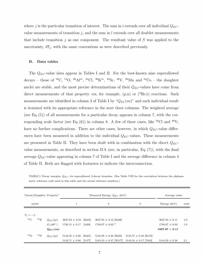
B. Data tables

The QEC-value data appear in Tables I and II. For the best-known nine superallowed

decays – those of 10C, 14O, 26Alm, 34Cl, 38Km, 42Sc, 46V, 50Mn and 54Co – the daughter

nuclei are stable, and the most precise determinations of their QEC-values have come from

direct measurements of that property via, for example, (p,n) or (3He,t) reactions. Such

measurements are identified in column 3 of Table I by “QEC(sa)” and each individual result

is itemized with its appropriate reference in the next three columns. The weighted average

(see Eq. (5)) of all measurements for a particular decay appears in column 7, with the cor-

responding scale factor (see Eq. (6)) in column 8. A few of these cases, like 34Cl and 46V,

have no further complications. There are other cases, however, in which QEC-value differ-

ences have been measured in addition to the individual QEC-values. These measurements

are presented in Table II. They have been dealt with in combination with the direct QEC-

value measurements, as described in section IIA (see, in particular, Eq. (7)), with the final

average QEC-value appearing in column 7 of Table I and the average difference in column 4

of Table II. Both are flagged with footnotes to indicate the interconnection.

TABLE I: Decay energies, QEC , for superallowed β-decay branches. (See Table VIII for the correlation between the alphanu-

meric reference code used in this table and the actual reference numbers.)

Parent/Daughter Property1 Measured Energy, QEC (keV) Average value

nuclei 1 2 3 Energy (keV) scale

Tz = −1:

10C 10B QEC(gs) 3647.84 ± 0.34 [Ba84] 3647.95 ± 0.12 [Ba98] 3647.94 ± 0.11 1.0

Ex(d0+) 1740.15 ± 0.17 [Aj88] 1740.07 ± 0.02 2 1740.07 ± 0.02 1.0

QEC (sa) 1907.87 ± 0.11

14O 14N QEC(gs) 5143.35 ± 0.60 [Bu61] 5145.09 ± 0.46 [Ba62] 5145.57 ± 0.48 [Ro70]

5142.71 ± 0.80 [Vo77] 5143.43 ± 0.37 [Wh77] 5144.34 ± 0.17 [To03] 5144.29 ± 0.28 2.1

7

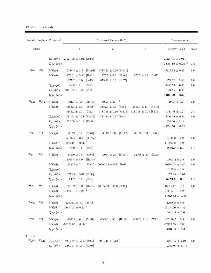
TABLE I (continued)

Parent/Daughter Property1 Measured Energy (keV) Average value

nuclei 1 2 3 Energy (keV) scale

Ex(d0+) 2312.798 ± 0.011 [Aj91] 2312.798 ± 0.011

QEC (sa) 2831.18 ± 0.24 3 2.5

18Ne 18F ME(p) 5316.8 ± 1.5 [Ma94] 5317.63 ± 0.36 [Bl04b] 5317.58 ± 0.35 1.0

ME(d) 873.31 ± 0.94 [Bo64] 875.5 ± 2.2 [Ho64] 876.5 ± 2.8 [Pr67]

877.2 ± 3.0 [Se73] 873.96 ± 0.61 [Ro75] 874.02 ± 0.48 1.0

QEC(gs) 4438 ± 9 [Fr63] 4443.54 ± 0.60 1.0

Ex(d0+) 1041.55 ± 0.08 [Ti95] 1041.55 ± 0.08

QEC (sa) 3401.99 ± 0.60

22Mg 22Na ME(p) -401.3 ± 3.0 [Ha74c] -400.5 ± 1.3 4 -400.6 ± 1.2 1.0

ME(d) -5184.3 ± 1.5 [We68] -5182.5 ± 0.5 [Be68] -5181.3 ± 1.7 [An70]

-5183.2 ± 1.0 [Gi72] -5181.56 ± 0.16 [Mu04] -5181.08 ± 0.30 [Sa04] -5181.58 ± 0.27 2.4

QEC(gs) 4781.64 ± 0.28 [Mu04] 4781.40 ± 0.67 [Sa04] 4781.58 ± 0.25 1.0

Ex(d0+) 657.00 ± 0.14 [En98] 657.00 ± 0.14

QEC (sa) 4124.58 ± 0.29

26Si 26Al ME(p) -7159 ± 18 [Mi67] -7149 ± 30 [Mc67] -7139 ± 30 [Ha68]

-7145.5 ± 3.0 [Ha74c] -7145.8 ± 2.9 1.0

ME(d0+) -11982.08 ± 0.26 5 -11982.08 ± 0.26

QEC (sa) 4850 ± 13 [Fr63] 4836.9 ± 3.0 1.0

30S 30P ME(p) -14060 ± 15 [Mi67] -14054 ± 25 [Mc67] -14068 ± 30 [Ha68]

-14063.4 ± 3.0 [Ha74c] -14063.2 ± 2.9 1.0

ME(d) -20203 ± 3 [Ha67] -20200.58 ± 0.40 [Re85] -20200.62 ± 0.40 1.0

QEC(gs) 6137.4 ± 2.9

Ex(d0+) 677.29 ± 0.07 [En98] 677.29 ± 0.07

QEC (sa) 5437 ± 17 [Fr63] 5459.5 ± 3.9 1.3

34Ar 34Cl ME(p) -18380.2 ± 3.0 [Ha74c] -18377.10 ± 0.41 [He02] -18377.17 ± 0.40 1.0

ME(d) -24440.01 ± 0.23 5 -24440.01 ± 0.23

QEC (sa) 6062.83 ± 0.46

38Ca 38K ME(p) -22056.0 ± 5.0 [Se74] -22056.0 ± 5.0

ME(d0+) -28670.20 ± 0.32 5 -28670.20 ± 0.32

QEC (sa) 6614.2 ± 5.0

42Ti 42Sc ME(p) -25121 ± 6 [Mi67] -25086 ± 30 [Ha68] -25124 ± 13 [Zi72] -25120.7 ± 5.3 1.0

ME(d) -32121.55 ± 0.80 5 -32121.55 ± 0.80

QEC (sa) 7000.9 ± 5.4

Tz = 0:

26Alm 26Mg QEC(gs) 4004.79 ± 0.55 [De69] 4004.41 ± 0.10 6 4004.42 ± 0.10 1.0

Ex(p0+) 228.305 ± 0.013 [En98] 228.305 ± 0.013

8

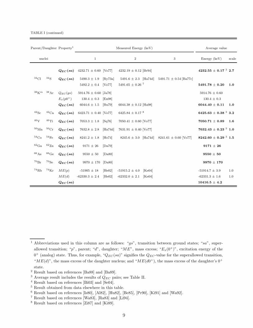
TABLE I (continued)

Parent/Daughter Property1 Measured Energy (keV) Average value

nuclei 1 2 3 Energy (keV) scale

QEC (sa) 4232.71 ± 0.60 [Vo77] 4232.19 ± 0.12 [Br94] 4232.55 ± 0.17 3 2.7

34Cl 34S QEC (sa) 5490.3 ± 1.9 [Ry73a] 5491.6 ± 2.3 [Ha74d] 5491.71 ± 0.54 [Ba77c]

5492.2 ± 0.4 [Vo77] 5491.65 ± 0.26 7 5491.78 ± 0.20 1.0

38Km 38Ar QEC(gs) 5914.76 ± 0.60 [Ja78] 5914.76 ± 0.60

Ex(p0+) 130.4 ± 0.3 [En98] 130.4 ± 0.3

QEC (sa) 6044.6 ± 1.5 [Bu79] 6044.38 ± 0.12 [Ha98] 6044.40 ± 0.11 1.0

42Sc 42Ca QEC (sa) 6423.71 ± 0.40 [Vo77] 6425.84 ± 0.17 8 6425.63 ± 0.38 3 3.2

46V 46Ti QEC (sa) 7053.3 ± 1.8 [Sq76] 7050.41 ± 0.60 [Vo77] 7050.71 ± 0.89 1.6

50Mn 50Cr QEC (sa) 7632.8 ± 2.8 [Ha74d] 7631.91 ± 0.40 [Vo77] 7632.43 ± 0.23 3 1.0

54Co 54Fe QEC (sa) 8241.2 ± 1.8 [Ho74] 8245.6 ± 3.0 [Ha74d] 8241.61 ± 0.60 [Vo77] 8242.60 ± 0.29 3 1.5

62Ga 62Zn QEC (sa) 9171 ± 26 [Da79] 9171 ± 26

66As 66Ge QEC (sa) 9550 ± 50 [Da80] 9550 ± 50

70Br 70Se QEC (sa) 9970 ± 170 [Da80] 9970 ± 170

74Rb 74Kr ME(p) -51905 ± 18 [He02] -51915.2 ± 4.0 [Ke04] -51914.7 ± 3.9 1.0

ME(d) -62330.3 ± 2.4 [He02] -62332.0 ± 2.1 [Ke04] -62331.3 ± 1.6 1.0

QEC (sa) 10416.5 ± 4.2

1 Abbreviations used in this column are as follows: “gs”, transition between ground states; “sa”, super-

allowed transition; “p”, parent; “d”, daughter; “ME”, mass excess; “Ex(0+)”, excitation energy of the

0+ (analog) state. Thus, for example, “QEC(sa)” signifies the QEC-value for the superallowed transition,

“ME(d)”, the mass excess of the daughter nucleus; and “ME(d0+), the mass excess of the daughter’s 0+

state.2 Result based on references [Ba88] and [Ba89].3 Average result includes the results of QEC pairs; see Table II.4 Result based on references [Bi03] and [Se04].5 Result obtained from data elsewhere in this table.6 Result based on references [Is80], [Al82], [Hu82], [Be85], [Pr90], [Ki91] and [Wa92].7 Result based on references [Wa83], [Ra83] and [Li94].8 Result based on references [Zi87] and [Ki89].

9

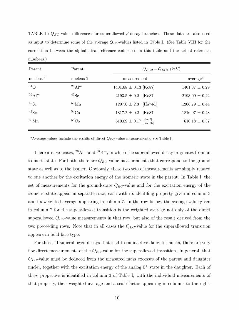
TABLE II: QEC-value differences for superallowed β-decay branches. These data are also used

as input to determine some of the average QEC-values listed in Table I. (See Table VIII for the

correlation between the alphabetical reference code used in this table and the actual reference

numbers.)

Parent Parent QEC2 −QEC1 (keV)

nucleus 1 nucleus 2 measurement averagea

14O 26Alm 1401.68 ± 0.13 [Ko87] 1401.37 ± 0.29

26Alm 42Sc 2193.5 ± 0.2 [Ko87] 2193.09 ± 0.42

42Sc 50Mn 1207.6 ± 2.3 [Ha74d] 1206.79 ± 0.44

42Sc 54Co 1817.2 ± 0.2 [Ko87] 1816.97 ± 0.48

50Mn 54Co 610.09 ± 0.17[Ko87][Ko97b] 610.18 ± 0.37

aAverage values include the results of direct QEC-value measurements: see Table I.

There are two cases, 26Alm and 38Km, in which the superallowed decay originates from an

isomeric state. For both, there are QEC-value measurements that correspond to the ground

state as well as to the isomer. Obviously, these two sets of measurements are simply related

to one another by the excitation energy of the isomeric state in the parent. In Table I, the

set of measurements for the ground-state QEC-value and for the excitation energy of the

isomeric state appear in separate rows, each with its identifing property given in column 3

and its weighted average appearing in column 7. In the row below, the average value given

in column 7 for the superallowed transition is the weighted average not only of the direct

superallowed QEC-value measurements in that row, but also of the result derived from the

two preceeding rows. Note that in all cases the QEC-value for the superallowed transition

appears in bold-face type.

For those 11 superallowed decays that lead to radioactive daughter nuclei, there are very

few direct measurements of the QEC-value for the superallowed transition. In general, that

QEC-value must be deduced from the measured mass excesses of the parent and daughter

nuclei, together with the excitation energy of the analog 0+ state in the daughter. Each of

these properties is identified in column 3 of Table I, with the individual measurements of

that property, their weighted average and a scale factor appearing in columns to the right.

10

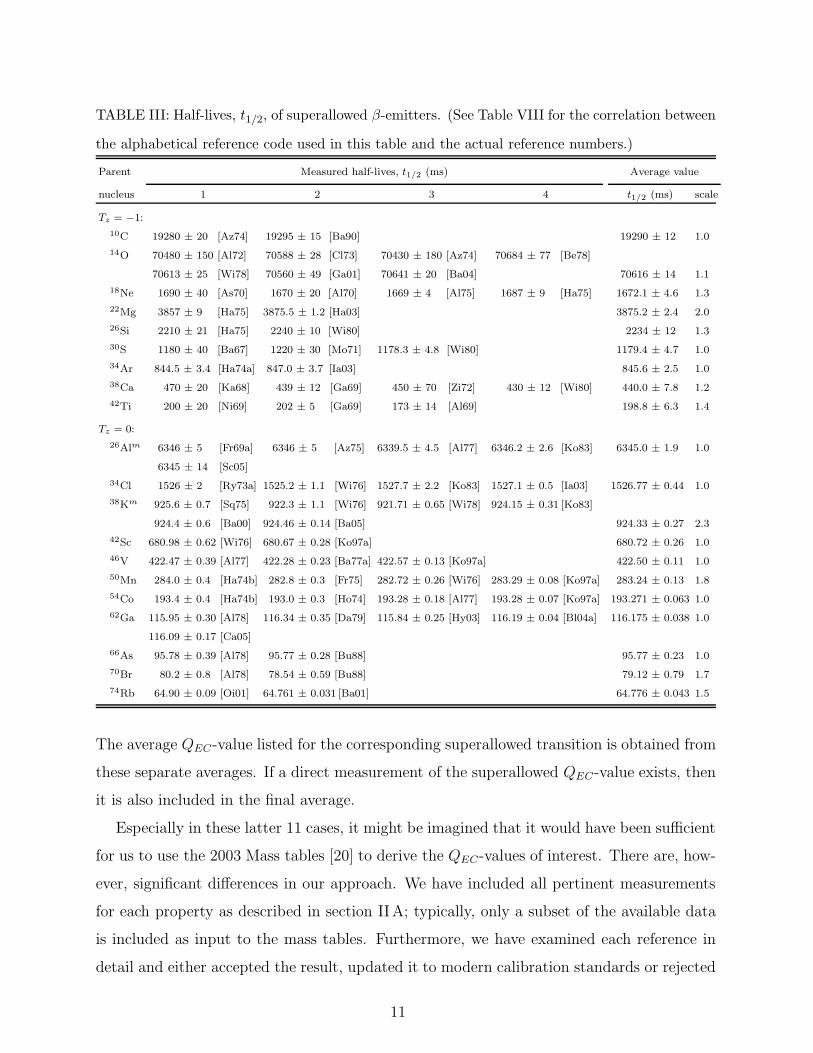
TABLE III: Half-lives, t1/2, of superallowed β-emitters. (See Table VIII for the correlation between

the alphabetical reference code used in this table and the actual reference numbers.)

Parent Measured half-lives, t1/2 (ms) Average value

nucleus 1 2 3 4 t1/2 (ms) scale

Tz = −1:

10C 19280 ± 20 [Az74] 19295 ± 15 [Ba90] 19290 ± 12 1.0

14O 70480 ± 150 [Al72] 70588 ± 28 [Cl73] 70430 ± 180 [Az74] 70684 ± 77 [Be78]

70613 ± 25 [Wi78] 70560 ± 49 [Ga01] 70641 ± 20 [Ba04] 70616 ± 14 1.1

18Ne 1690 ± 40 [As70] 1670 ± 20 [Al70] 1669 ± 4 [Al75] 1687 ± 9 [Ha75] 1672.1 ± 4.6 1.3

22Mg 3857 ± 9 [Ha75] 3875.5 ± 1.2 [Ha03] 3875.2 ± 2.4 2.0

26Si 2210 ± 21 [Ha75] 2240 ± 10 [Wi80] 2234 ± 12 1.3

30S 1180 ± 40 [Ba67] 1220 ± 30 [Mo71] 1178.3 ± 4.8 [Wi80] 1179.4 ± 4.7 1.0

34Ar 844.5 ± 3.4 [Ha74a] 847.0 ± 3.7 [Ia03] 845.6 ± 2.5 1.0

38Ca 470 ± 20 [Ka68] 439 ± 12 [Ga69] 450 ± 70 [Zi72] 430 ± 12 [Wi80] 440.0 ± 7.8 1.2

42Ti 200 ± 20 [Ni69] 202 ± 5 [Ga69] 173 ± 14 [Al69] 198.8 ± 6.3 1.4

Tz = 0:

26Alm 6346 ± 5 [Fr69a] 6346 ± 5 [Az75] 6339.5 ± 4.5 [Al77] 6346.2 ± 2.6 [Ko83] 6345.0 ± 1.9 1.0

6345 ± 14 [Sc05]

34Cl 1526 ± 2 [Ry73a] 1525.2 ± 1.1 [Wi76] 1527.7 ± 2.2 [Ko83] 1527.1 ± 0.5 [Ia03] 1526.77 ± 0.44 1.0

38Km 925.6 ± 0.7 [Sq75] 922.3 ± 1.1 [Wi76] 921.71 ± 0.65 [Wi78] 924.15 ± 0.31 [Ko83]

924.4 ± 0.6 [Ba00] 924.46 ± 0.14 [Ba05] 924.33 ± 0.27 2.3

42Sc 680.98 ± 0.62 [Wi76] 680.67 ± 0.28 [Ko97a] 680.72 ± 0.26 1.0

46V 422.47 ± 0.39 [Al77] 422.28 ± 0.23 [Ba77a] 422.57 ± 0.13 [Ko97a] 422.50 ± 0.11 1.0

50Mn 284.0 ± 0.4 [Ha74b] 282.8 ± 0.3 [Fr75] 282.72 ± 0.26 [Wi76] 283.29 ± 0.08 [Ko97a] 283.24 ± 0.13 1.8

54Co 193.4 ± 0.4 [Ha74b] 193.0 ± 0.3 [Ho74] 193.28 ± 0.18 [Al77] 193.28 ± 0.07 [Ko97a] 193.271 ± 0.063 1.0

62Ga 115.95 ± 0.30 [Al78] 116.34 ± 0.35 [Da79] 115.84 ± 0.25 [Hy03] 116.19 ± 0.04 [Bl04a] 116.175 ± 0.038 1.0

116.09 ± 0.17 [Ca05]

66As 95.78 ± 0.39 [Al78] 95.77 ± 0.28 [Bu88] 95.77 ± 0.23 1.0

70Br 80.2 ± 0.8 [Al78] 78.54 ± 0.59 [Bu88] 79.12 ± 0.79 1.7

74Rb 64.90 ± 0.09 [Oi01] 64.761 ± 0.031 [Ba01] 64.776 ± 0.043 1.5

The average QEC-value listed for the corresponding superallowed transition is obtained from

these separate averages. If a direct measurement of the superallowed QEC-value exists, then

it is also included in the final average.

Especially in these latter 11 cases, it might be imagined that it would have been sufficient

for us to use the 2003 Mass tables [20] to derive the QEC-values of interest. There are, how-

ever, significant differences in our approach. We have included all pertinent measurements

for each property as described in section IIA; typically, only a subset of the available data

is included as input to the mass tables. Furthermore, we have examined each reference in

detail and either accepted the result, updated it to modern calibration standards or rejected

11

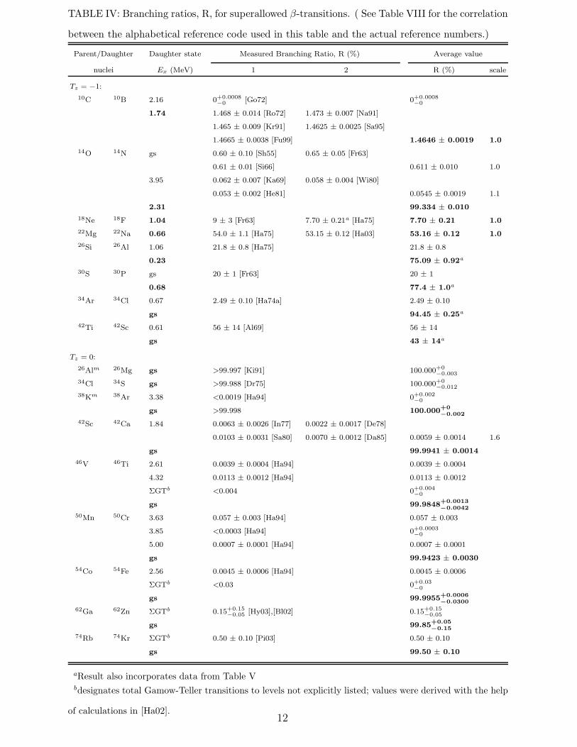
TABLE IV: Branching ratios, R, for superallowed β-transitions. ( See Table VIII for the correlation

between the alphabetical reference code used in this table and the actual reference numbers.)

Parent/Daughter Daughter state Measured Branching Ratio, R (%) Average value

nuclei Ex (MeV) 1 2 R (%) scale

Tz = −1:

10C 10B 2.16 0+0.0008−0

[Go72] 0+0.0008−0

1.74 1.468 ± 0.014 [Ro72] 1.473 ± 0.007 [Na91]

1.465 ± 0.009 [Kr91] 1.4625 ± 0.0025 [Sa95]

1.4665 ± 0.0038 [Fu99] 1.4646 ± 0.0019 1.0

14O 14N gs 0.60 ± 0.10 [Sh55] 0.65 ± 0.05 [Fr63]

0.61 ± 0.01 [Si66] 0.611 ± 0.010 1.0

3.95 0.062 ± 0.007 [Ka69] 0.058 ± 0.004 [Wi80]

0.053 ± 0.002 [He81] 0.0545 ± 0.0019 1.1

2.31 99.334 ± 0.010

18Ne 18F 1.04 9 ± 3 [Fr63] 7.70 ± 0.21a [Ha75] 7.70 ± 0.21 1.0

22Mg 22Na 0.66 54.0 ± 1.1 [Ha75] 53.15 ± 0.12 [Ha03] 53.16 ± 0.12 1.0

26Si 26Al 1.06 21.8 ± 0.8 [Ha75] 21.8 ± 0.8

0.23 75.09 ± 0.92a

30S 30P gs 20 ± 1 [Fr63] 20 ± 1

0.68 77.4 ± 1.0a

34Ar 34Cl 0.67 2.49 ± 0.10 [Ha74a] 2.49 ± 0.10

gs 94.45 ± 0.25a

42Ti 42Sc 0.61 56 ± 14 [Al69] 56 ± 14

gs 43 ± 14a

Tz = 0:

26Alm 26Mg gs >99.997 [Ki91] 100.000+0−0.003

34Cl 34S gs >99.988 [Dr75] 100.000+0−0.012

38Km 38Ar 3.38 <0.0019 [Ha94] 0+0.002−0

gs >99.998 100.000+0

−0.002

42Sc 42Ca 1.84 0.0063 ± 0.0026 [In77] 0.0022 ± 0.0017 [De78]

0.0103 ± 0.0031 [Sa80] 0.0070 ± 0.0012 [Da85] 0.0059 ± 0.0014 1.6

gs 99.9941 ± 0.0014

46V 46Ti 2.61 0.0039 ± 0.0004 [Ha94] 0.0039 ± 0.0004

4.32 0.0113 ± 0.0012 [Ha94] 0.0113 ± 0.0012

ΣGTb <0.004 0+0.004−0

gs 99.9848+0.0013

−0.0042

50Mn 50Cr 3.63 0.057 ± 0.003 [Ha94] 0.057 ± 0.003

3.85 <0.0003 [Ha94] 0+0.0003−0

5.00 0.0007 ± 0.0001 [Ha94] 0.0007 ± 0.0001

gs 99.9423 ± 0.0030

54Co 54Fe 2.56 0.0045 ± 0.0006 [Ha94] 0.0045 ± 0.0006

ΣGTb <0.03 0+0.03−0

gs 99.9955+0.0006

−0.0300

62Ga 62Zn ΣGTb 0.15+0.15−0.05 [Hy03],[Bl02] 0.15+0.15

−0.05

gs 99.85+0.05

−0.15

74Rb 74Kr ΣGTb 0.50 ± 0.10 [Pi03] 0.50 ± 0.10

gs 99.50 ± 0.10

aResult also incorporates data from Table Vbdesignates total Gamow-Teller transitions to levels not explicitly listed; values were derived with the help

of calculations in [Ha02].12

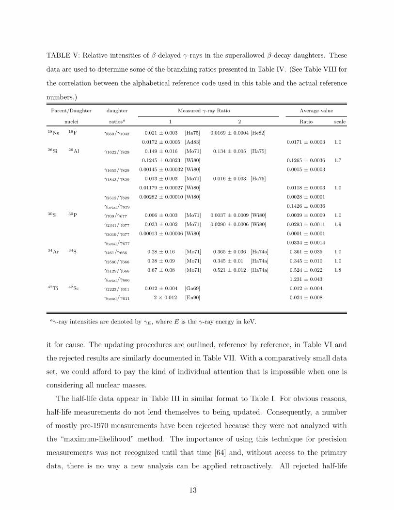
TABLE V: Relative intensities of β-delayed γ-rays in the superallowed β-decay daughters. These

data are used to determine some of the branching ratios presented in Table IV. (See Table VIII for

the correlation between the alphabetical reference code used in this table and the actual reference

numbers.)

Parent/Daughter daughter Measured γ-ray Ratio Average value

nuclei ratiosa 1 2 Ratio scale

18Ne 18F γ660/γ1042 0.021 ± 0.003 [Ha75] 0.0169 ± 0.0004 [He82]

0.0172 ± 0.0005 [Ad83] 0.0171 ± 0.0003 1.0

26Si 26Al γ1622/γ829 0.149 ± 0.016 [Mo71] 0.134 ± 0.005 [Ha75]

0.1245 ± 0.0023 [Wi80] 0.1265 ± 0.0036 1.7

γ1655/γ829 0.00145 ± 0.00032 [Wi80] 0.0015 ± 0.0003

γ1843/γ829 0.013 ± 0.003 [Mo71] 0.016 ± 0.003 [Ha75]

0.01179 ± 0.00027 [Wi80] 0.0118 ± 0.0003 1.0

γ2512/γ829 0.00282 ± 0.00010 [Wi80] 0.0028 ± 0.0001

γtotal/γ829 0.1426 ± 0.0036

30S 30P γ709/γ677 0.006 ± 0.003 [Mo71] 0.0037 ± 0.0009 [Wi80] 0.0039 ± 0.0009 1.0

γ2341/γ677 0.033 ± 0.002 [Mo71] 0.0290 ± 0.0006 [Wi80] 0.0293 ± 0.0011 1.9

γ3019/γ677 0.00013 ± 0.00006 [Wi80] 0.0001 ± 0.0001

γtotal/γ677 0.0334 ± 0.0014

34Ar 34S γ461/γ666 0.28 ± 0.16 [Mo71] 0.365 ± 0.036 [Ha74a] 0.361 ± 0.035 1.0

γ2580/γ666 0.38 ± 0.09 [Mo71] 0.345 ± 0.01 [Ha74a] 0.345 ± 0.010 1.0

γ3129/γ666 0.67 ± 0.08 [Mo71] 0.521 ± 0.012 [Ha74a] 0.524 ± 0.022 1.8

γtotal/γ666 1.231 ± 0.043

42Ti 42Sc γ2223/γ611 0.012 ± 0.004 [Ga69] 0.012 ± 0.004

γtotal/γ611 2 × 0.012 [En90] 0.024 ± 0.008

aγ-ray intensities are denoted by γE , where E is the γ-ray energy in keV.

it for cause. The updating procedures are outlined, reference by reference, in Table VI and

the rejected results are similarly documented in Table VII. With a comparatively small data

set, we could afford to pay the kind of individual attention that is impossible when one is

considering all nuclear masses.

The half-life data appear in Table III in similar format to Table I. For obvious reasons,

half-life measurements do not lend themselves to being updated. Consequently, a number

of mostly pre-1970 measurements have been rejected because they were not analyzed with

the “maximum-likelihood” method. The importance of using this technique for precision

measurements was not recognized until that time [64] and, without access to the primary

data, there is no way a new analysis can be applied retroactively. All rejected half-life

13

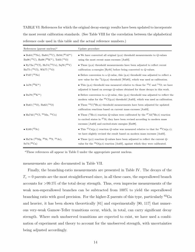
TABLE VI: References for which the original decay-energy results have been updated to incorporate

the most recent calibration standards. (See Table VIII for the correlation between the alphabetical

reference code used in this table and the actual reference numbers.)

References (parent nucleus)a Update procedure

• Bo64 (18Ne), Ba84 (10C), Br94 (26Alm) • We have converted all original (p,n) threshold measurements to Q-values

Ba98 (10C), Ha98 (38Km), To03 (14O) using the most recent mass excesses [Au03].

• Ry73a (34Cl), Ho74 (54Co), Sq76 (46V) • These (p,n) threshold measurements have been adjusted to reflect recent

Ba77c (34Cl), Wh77 (14O) calibration α-energies [Ry91] before being converted to Q-values.

• Pr67 (18Ne) • Before conversion to a Q-value, this (p,n) threshold was adjusted to reflect a

new value for the 7Li(p,n) threshold [Wh85], which was used as calibration.

• Ja78 (38Km) • This (p,n) threshold was measured relative to those for 10C and 14O; we have

adjusted it based on average Q-values obtained for those decays in this work.

• Bu79 (38Km) • Before conversion to a Q-value, this (p,n) threshold was adjusted to reflect the

modern value for the 35Cl(p,n) threshold [Au03], which was used as calibration.

• Bu61 (14O), Ba62 (14O) • These 12C(3He,n) threshold measurements have been adjusted for updated

calibration reactions based on current mass excesses [Au03].

• Ha74d (34Cl, 50Mn, 54Co) • These (3He,t) reaction Q-values were calibrated by the 27Al(3He,t) reaction

to excited states in 27Si; they have been revised according to modern mass

excesses [Au03] and excited-state energies [En98].

• Ki89 (42Sc) • This 41Ca(p,γ) reaction Q-value was measured relative to that for 40Ca(p,γ);

we have slightly revised the result based on modern mass excesses [Au03].

• Ha74c (22Mg, 26Si, 30S, 34Ar), • These (p,t) reaction Q-values have been adjusted to reflect the current Q-

Se74 (38Ca) value for the 16O(p,t) reaction [Au03], against which they were calibrated.

aThese references all appear in Table I under the appropriate parent nucleus.

measurements are also documented in Table VII.

Finally, the branching-ratio measurements are presented in Table IV. The decays of the

Tz = 0 parents are the most straightforward since, in all these cases, the superallowed branch

accounts for >99.5% of the total decay strength. Thus, even imprecise measurements of the

weak non-superallowed branches can be subtracted from 100% to yield the superallowed

branching ratio with good precision. For the higher-Z parents of this type, particularly 62Ga

and heavier, it has been shown theoretically [81] and experimentally [90, 117] that numer-

ous very-weak Gamow-Teller transitions occur, which, in total, can carry significant decay

strength. Where such unobserved transitions are expected to exist, we have used a combi-

nation of experiment and theory to account for the unobserved strength, with uncertainties

being adjusted accordingly.

14

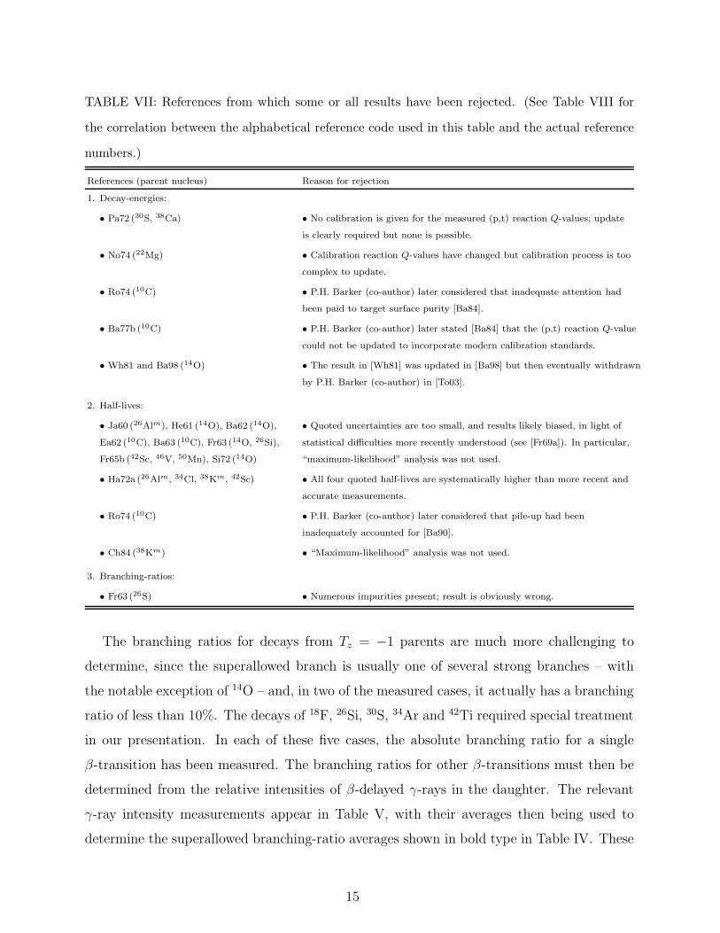
TABLE VII: References from which some or all results have been rejected. (See Table VIII for

the correlation between the alphabetical reference code used in this table and the actual reference

numbers.)

References (parent nucleus) Reason for rejection

1. Decay-energies:

• Pa72 (30S, 38Ca) • No calibration is given for the measured (p,t) reaction Q-values; update

is clearly required but none is possible.

• No74 (22Mg) • Calibration reaction Q-values have changed but calibration process is too

complex to update.

• Ro74 (10C) • P.H. Barker (co-author) later considered that inadequate attention had

been paid to target surface purity [Ba84].

• Ba77b (10C) • P.H. Barker (co-author) later stated [Ba84] that the (p,t) reaction Q-value

could not be updated to incorporate modern calibration standards.

• Wh81 and Ba98 (14O) • The result in [Wh81] was updated in [Ba98] but then eventually withdrawn

by P.H. Barker (co-author) in [To03].

2. Half-lives:

• Ja60 (26Alm), He61 (14O), Ba62 (14O), • Quoted uncertainties are too small, and results likely biased, in light of

Ea62 (10C), Ba63 (10C), Fr63 (14O, 26Si), statistical difficulties more recently understood (see [Fr69a]). In particular,

Fr65b (42Sc, 46V, 50Mn), Si72 (14O) “maximum-likelihood” analysis was not used.

• Ha72a (26Alm, 34Cl, 38Km, 42Sc) • All four quoted half-lives are systematically higher than more recent and

accurate measurements.

• Ro74 (10C) • P.H. Barker (co-author) later considered that pile-up had been

inadequately accounted for [Ba90].

• Ch84 (38Km) • “Maximum-likelihood” analysis was not used.

3. Branching-ratios:

• Fr63 (26S) • Numerous impurities present; result is obviously wrong.

The branching ratios for decays from Tz = −1 parents are much more challenging to

determine, since the superallowed branch is usually one of several strong branches – with

the notable exception of 14O – and, in two of the measured cases, it actually has a branching

ratio of less than 10%. The decays of 18F, 26Si, 30S, 34Ar and 42Ti required special treatment

in our presentation. In each of these five cases, the absolute branching ratio for a single

β-transition has been measured. The branching ratios for other β-transitions must then be

determined from the relative intensities of β-delayed γ-rays in the daughter. The relevant

γ-ray intensity measurements appear in Table V, with their averages then being used to

determine the superallowed branching-ratio averages shown in bold type in Table IV. These

15

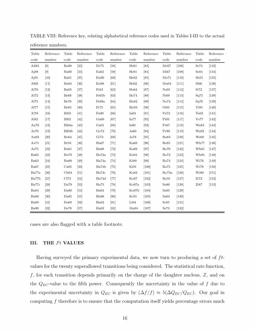
TABLE VIII: Reference key, relating alphabetical reference codes used in Tables I-III to the actual

reference numbers.

Table Reference Table Reference Table Reference Table Reference Table Reference Table Reference

code number code number code number code number code number code number

Ad83 [8] Ba98 [33] Dr75 [58] He61 [83] Mc67 [108] Se74 [133]

Aj88 [9] Ba00 [34] Ea62 [59] He81 [84] Mi67 [109] Se04 [134]

Aj91 [10] Ba01 [35] En90 [60] He82 [85] Mo71 [110] Sh55 [135]

Al69 [11] Ba04 [36] En98 [61] He02 [86] Mu04 [111] Si66 [136]

Al70 [12] Ba05 [37] Fr63 [62] Ho64 [87] Na91 [112] Si72 [137]

Al72 [13] Be68 [38] Fr65b [63] Ho74 [88] Ni69 [113] Sq75 [138]

Al75 [14] Be78 [39] Fr69a [64] Hu82 [89] No74 [114] Sq76 [139]

Al77 [15] Be85 [40] Fr75 [65] Hy03 [90] Oi01 [115] Ti95 [140]

Al78 [16] Bi03 [41] Fu99 [66] Ia03 [91] Pa72 [116] To03 [141]

Al82 [17] Bl02 [42] Ga69 [67] In77 [92] Pi03 [117] Vo77 [142]

An70 [18] Bl04a [43] Ga01 [68] Is80 [93] Pr67 [118] Wa83 [143]

As70 [19] Bl04b [44] Go72 [70] Ja60 [94] Pr90 [119] Wa92 [144]

Au03 [20] Bo64 [45] Gi72 [69] Ja78 [95] Ra83 [120] We68 [145]

Az74 [21] Br94 [46] Ha67 [71] Ka68 [96] Re85 [121] Wh77 [146]

Az75 [22] Bu61 [47] Ha68 [72] Ka69 [97] Ro70 [122] Wh81 [147]

Ba62 [23] Bu79 [48] Ha72a [73] Ke04 [98] Ro72 [123] Wh85 [148]

Ba63 [24] Bu88 [49] Ha74a [74] Ki89 [99] Ro74 [124] Wi76 [149]

Ba67 [25] Ca05 [50] Ha74b [75] Ki91 [100] Ro75 [125] Wi78 [150]

Ba77a [26] Ch84 [51] Ha74c [76] Ko83 [101] Ry73a [126] Wi80 [151]

Ba77b [27] Cl73 [52] Ha74d [77] Ko87 [102] Ry91 [127] Zi72 [152]

Ba77c [28] Da79 [53] Ha75 [78] Ko97a [103] Sa80 [128] Zi87 [153]

Ba84 [29] Da80 [54] Ha94 [79] Ko97b [104] Sa95 [129]

Ba88 [30] Da85 [55] Ha98 [80] Kr91 [105] Sa04 [130]

Ba89 [31] De69 [56] Ha02 [81] Li94 [106] Sc05 [131]

Ba90 [32] De78 [57] Ha03 [82] Ma94 [107] Se73 [132]

cases are also flagged with a table footnote.

III. THE Ft VALUES

Having surveyed the primary experimental data, we now turn to producing a set of ft-

values for the twenty superallowed transitions being considered. The statistical rate function,

f , for each transition depends primarily on the charge of the daughter nucleus, Z, and on

the QEC-value to the fifth power. Consequently the uncertainty in the value of f due to

the experimental uncertainty in QEC is given by (∆f/f) ≈ 5(∆QEC/QEC). Our goal in

computing f therefore is to ensure that the computation itself yields percentage errors much

16

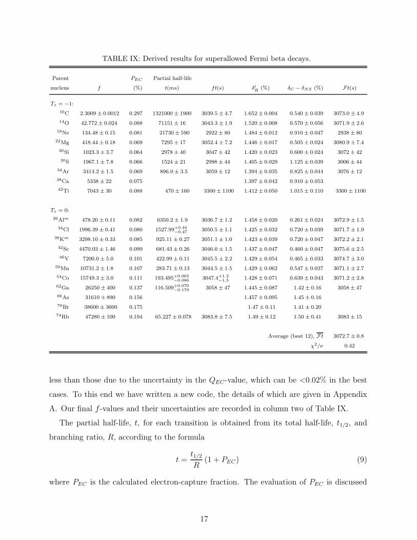
TABLE IX: Derived results for superallowed Fermi beta decays.

Parent PEC Partial half-life

nucleus f (%) t(ms) ft(s) δ′R (%) δC − δNS (%) Ft(s)

Tz = −1:

10C 2.3009 ± 0.0012 0.297 1321000 ± 1900 3039.5 ± 4.7 1.652 ± 0.004 0.540 ± 0.039 3073.0 ± 4.9

14O 42.772± 0.024 0.088 71151 ± 16 3043.3 ± 1.9 1.520 ± 0.008 0.570 ± 0.056 3071.9 ± 2.6

18Ne 134.48 ± 0.15 0.081 21730 ± 590 2922 ± 80 1.484 ± 0.012 0.910 ± 0.047 2938 ± 80

22Mg 418.44 ± 0.18 0.069 7295 ± 17 3052.4 ± 7.2 1.446 ± 0.017 0.505 ± 0.024 3080.9 ± 7.4

26Si 1023.3 ± 3.7 0.064 2978 ± 40 3047 ± 42 1.420 ± 0.023 0.600 ± 0.024 3072 ± 42

30S 1967.1 ± 7.8 0.066 1524 ± 21 2998 ± 44 1.405 ± 0.029 1.125 ± 0.039 3006 ± 44

34Ar 3414.2 ± 1.5 0.069 896.0± 3.5 3059 ± 12 1.394 ± 0.035 0.825 ± 0.044 3076 ± 12

38Ca 5338 ± 22 0.075 1.397 ± 0.042 0.910 ± 0.053

42Ti 7043 ± 30 0.088 470 ± 160 3300 ± 1100 1.412 ± 0.050 1.015 ± 0.110 3300 ± 1100

Tz = 0:

26Alm 478.20 ± 0.11 0.082 6350.2 ± 1.9 3036.7 ± 1.2 1.458 ± 0.020 0.261 ± 0.024 3072.9 ± 1.5

34Cl 1996.39 ± 0.41 0.080 1527.99+0.44−0.47 3050.5 ± 1.1 1.425 ± 0.032 0.720 ± 0.039 3071.7 ± 1.9

38Km 3298.10 ± 0.33 0.085 925.11 ± 0.27 3051.1 ± 1.0 1.423 ± 0.039 0.720 ± 0.047 3072.2 ± 2.1

42Sc 4470.03 ± 1.46 0.099 681.43 ± 0.26 3046.0 ± 1.5 1.437 ± 0.047 0.460 ± 0.047 3075.6 ± 2.5

46V 7200.0 ± 5.0 0.101 422.99 ± 0.11 3045.5 ± 2.2 1.429 ± 0.054 0.465 ± 0.033 3074.7 ± 3.0

50Mn 10731.2 ± 1.8 0.107 283.71 ± 0.13 3044.5 ± 1.5 1.429 ± 0.062 0.547 ± 0.037 3071.1 ± 2.7

54Co 15749.3 ± 3.0 0.111 193.495+0.063−0.086 3047.4+1.2

−1.5 1.428 ± 0.071 0.639 ± 0.043 3071.2 ± 2.8

62Ga 26250 ± 400 0.137 116.509+0.070−0.179 3058 ± 47 1.445 ± 0.087 1.42 ± 0.16 3058 ± 47

66As 31610 ± 890 0.156 1.457 ± 0.095 1.45 ± 0.16

70Br 38600 ± 3600 0.175 1.47± 0.11 1.41 ± 0.20

74Rb 47280 ± 100 0.194 65.227± 0.078 3083.8 ± 7.5 1.49± 0.12 1.50 ± 0.41 3083 ± 15

Average (best 12), Ft 3072.7 ± 0.8

χ2/ν 0.42

less than those due to the uncertainty in the QEC-value, which can be <0.02% in the best

cases. To this end we have written a new code, the details of which are given in Appendix

A. Our final f -values and their uncertainties are recorded in column two of Table IX.

The partial half-life, t, for each transition is obtained from its total half-life, t1/2, and

branching ratio, R, according to the formula

t =t1/2R

(1 + PEC) (9)

where PEC is the calculated electron-capture fraction. The evaluation of PEC is discussed

17

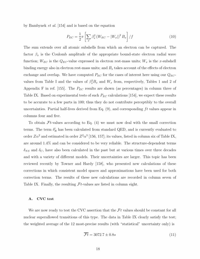
by Bambynek et al. [154] and is based on the equation

PEC =1

2π

[

∑

x

β2x (WEC − |Wx|)2Bx

]

/f (10)

The sum extends over all atomic subshells from which an electron can be captured. The

factor βx is the Coulomb amplitude of the appropriate bound-state electron radial wave

function; WEC is the QEC-value expressed in electron rest-mass units; Wx is the x-subshell

binding energy also in electron rest-mass units; and Bx takes account of the effects of electron

exchange and overlap. We have computed PEC for the cases of interest here using our QEC-

values from Table I and the values of β2xBx and Wx from, respectively, Tables 1 and 2 of

Appendix F in ref. [155]. The PEC results are shown (as percentages) in column three of

Table IX. Based on experimental tests of such PEC calculations [154], we expect these results

to be accurate to a few parts in 100; thus they do not contribute perceptibly to the overall

uncertainties. Partial half-lives derived from Eq. (9), and corresponding ft values appear in

columns four and five.

To obtain Ft-values according to Eq. (4) we must now deal with the small correction

terms. The term δ′R has been calculated from standard QED, and is currently evaluated to

order Zα2 and estimated in order Z2α3 [156, 157]; its values, listed in column six of Table IX,

are around 1.4% and can be considered to be very reliable. The structure-dependent terms

δNS and δC , have also been calculated in the past but at various times over three decades

and with a variety of different models. Their uncertainties are larger. This topic has been

reviewed recently by Towner and Hardy [158], who presented new calculations of these

corrections in which consistent model spaces and approximations have been used for both

correction terms. The results of these new calculations are recorded in column seven of

Table IX. Finally, the resulting Ft-values are listed in column eight.

A. CVC test

We are now ready to test the CVC assertion that the Ft values should be constant for all

nuclear superallowed transitions of this type. The data in Table IX clearly satisfy the test;

the weighted average of the 12 most-precise results (with “statistical” uncertainty only) is

Ft = 3072.7± 0.8s (11)

18

10 30203060

3100

3090

3080

3070

Z of daughter

t (s)

10C 14

O

22Mg

26 mAl 34

Cl

34Ar

38 mK

42Sc 46

V

50Mn

54Co

74Rb

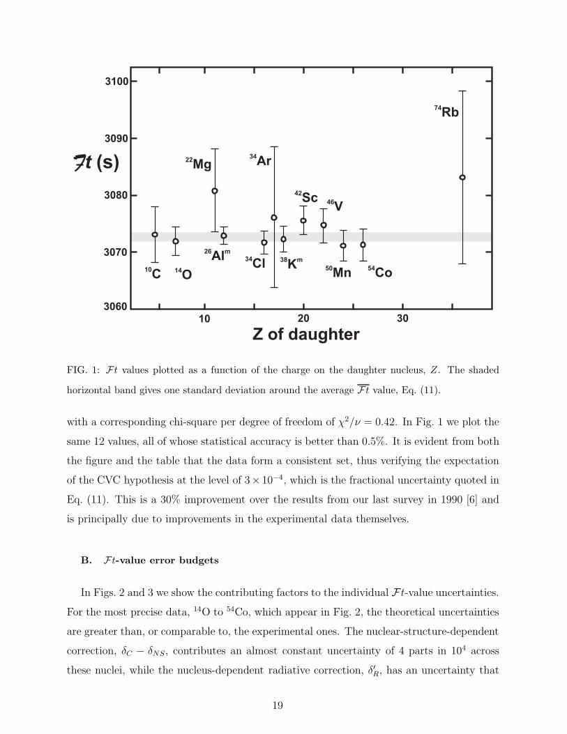
FIG. 1: Ft values plotted as a function of the charge on the daughter nucleus, Z. The shaded

horizontal band gives one standard deviation around the average Ft value, Eq. (11).

with a corresponding chi-square per degree of freedom of χ2/ν = 0.42. In Fig. 1 we plot the

same 12 values, all of whose statistical accuracy is better than 0.5%. It is evident from both

the figure and the table that the data form a consistent set, thus verifying the expectation

of the CVC hypothesis at the level of 3×10−4, which is the fractional uncertainty quoted in

Eq. (11). This is a 30% improvement over the results from our last survey in 1990 [6] and

is principally due to improvements in the experimental data themselves.

B. Ft-value error budgets

In Figs. 2 and 3 we show the contributing factors to the individual Ft-value uncertainties.For the most precise data, 14O to 54Co, which appear in Fig. 2, the theoretical uncertainties

are greater than, or comparable to, the experimental ones. The nuclear-structure-dependent

correction, δC − δNS, contributes an almost constant uncertainty of 4 parts in 104 across

these nuclei, while the nucleus-dependent radiative correction, δ′R, has an uncertainty that

19

10C

14O

26Al

m 34Cl

38K

m 42Sc

46V

50Mn

54Co

Part

s in

10

4

2

10

8

6

4

0

14

12Q-value

Half-life

Branching ratio

dR’

d dC NS-

Parent nucleus

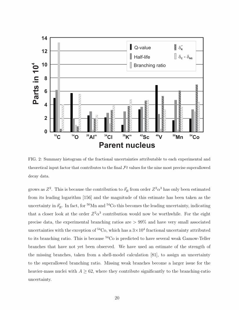
FIG. 2: Summary histogram of the fractional uncertainties attributable to each experimental and

theoretical input factor that contributes to the final Ft values for the nine most precise superallowed

decay data.

grows as Z2. This is because the contribution to δ′R from order Z2α3 has only been estimated

from its leading logarithm [156] and the magnitude of this estimate has been taken as the

uncertainty in δ′R. In fact, for 50Mn and 54Co this becomes the leading uncertainty, indicating

that a closer look at the order Z2α3 contribution would now be worthwhile. For the eight

precise data, the experimental branching ratios are > 99% and have very small associated

uncertainties with the exception of 54Co, which has a 3×104 fractional uncertainty attributed

to its branching ratio. This is because 54Co is predicted to have several weak Gamow-Teller

branches that have not yet been observed. We have used an estimate of the strength of

the missing branches, taken from a shell-model calculation [81], to assign an uncertainty

to the superallowed branching ratio. Missing weak branches become a larger issue for the

heavier-mass nuclei with A ≥ 62, where they contribute significantly to the branching-ratio

uncertainty.

20

T = 0Z

Part

s in

10

4

20

0

60

40

18Ne

42Ti

38Ca

34Ar

30S

26Si

22Mg

62Ga

74Rb

70Br

66As

Parent nucleus

T = -1Z

Q-value

Half-life

Branching ratio

dR’

d dC NS-0

20

40

60

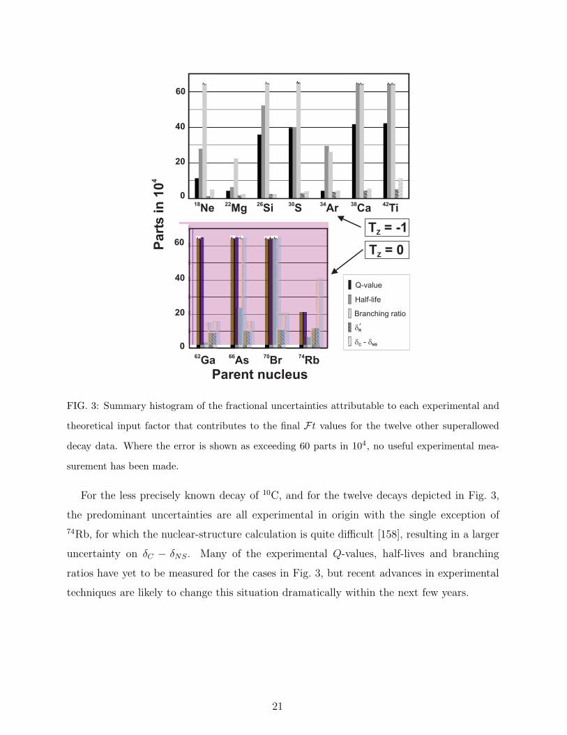
FIG. 3: Summary histogram of the fractional uncertainties attributable to each experimental and

theoretical input factor that contributes to the final Ft values for the twelve other superallowed

decay data. Where the error is shown as exceeding 60 parts in 104, no useful experimental mea-

surement has been made.

For the less precisely known decay of 10C, and for the twelve decays depicted in Fig. 3,

the predominant uncertainties are all experimental in origin with the single exception of

74Rb, for which the nuclear-structure calculation is quite difficult [158], resulting in a larger

uncertainty on δC − δNS. Many of the experimental Q-values, half-lives and branching

ratios have yet to be measured for the cases in Fig. 3, but recent advances in experimental

techniques are likely to change this situation dramatically within the next few years.

21

C. Accounting for systematic uncertainties

So far, we have dealt with the inter-nuclear behavior of Ft-values, examining their con-

stancy as a test of CVC. With that test passed at high precision, we are now in a position to

use the average Ft-value obtained from these concordant nuclear data to go beyond nuclei,

obtaining first the vector coupling constant (see Eq. (2)) and then the Vud matrix element.

Before doing so, however, we must address one more possible source of uncertainty. Though

the average Ft value given in Eq. (11) includes a full assessment of the uncertainties at-

tributable to experiment and to the particular calculations used to obtain the correction

terms, it does not incorporate any provision for a common systematic error that could arise

from the type of calculation chosen to model the nuclear-structure effects. In this section

we look more critically at the nuclear-structure-dependent corrections, and in particular at

the isospin-symmetry-breaking correction1, δC .

There have been a number of previous calculations of δC besides those of ours [158]:

Hartree-Fock calculations of Ormand and Brown [159], RPA calculations of Sagawa, van

Giai and Suzuki [160], R-matrix calculations of Barker [161], and Woods-Saxon calculations

of Wilkinson [162], to name some of the more recent publications. Of these, we will only

retain the Ormand-Brown (OB) calculations since they, like ours (TH), are constrained to

reproduce other isospin properties of the nuclei involved: They reproduce the measured

coefficients of the relevant isobaric multiplet mass equation, the known proton and neutron

separation energies, and the measured ft values of weak non-analog 0+ → 0+ transitions

[79], where they are known. The other calculations are not constrained by experiment in

any way and thus offer no independent means to assess their efficacy.

Unfortunately, calculations of δC by OB are not available for all the cases listed in Ta-

ble IX, so we must concentrate on the nine most precise data: 10C, 14O, 26Alm, 34Cl, 38Km,

42Sc, 46V, 50Mn, and 54Co. When the TH values of δC are used, the average Ft-value for

these nine cases alone is Ft = 3072.6± 0.8 s with χ2/ν = 0.35. When OB values are used

for δC instead, the weighted average is Ft = 3074.5 ± 0.8 s with χ2/ν = 0.92. Although

the chi-square with the OB values is nearly a factor of three worse, we do not argue that

1 The reason we do not consider further the nuclear-structure-dependent radiative correction, δNS , is that

it is very small for the series of transitions that have Tz = 0 parent states [158]. Of the nine precisely

known transitions we are concentrating on, seven are of this type.

22

this is sufficient reason to reject the OB calculation. Rather, we observe that the OB values

of δC are systematically smaller and hence the Ft values systematically larger than ours.

Evidently there is a systematic difference between our Woods-Saxon and OB’s Hartree-Fock

calculations of δC and that difference should be accounted for in the final result. Thus, we

adopt the average of these two results for our recommended Ft, and assign a systematic

uncertainty equal to half the spread between them: viz

Ft = 3073.5± 0.8stat ± 0.9syst s

= 3073.5± 1.2 s, (12)

where the two errors have been combined in quadrature.

IV. IMPACT ON WEAK-INTERACTION PHYSICS

A. The Value of Vud

With a mutually consistent set of Ft values, we can now use their average value in

Eq. (12) to determine the vector coupling constant, GV, from Eq. (2). The value of GV itself

is of little interest, but it can be related to the weak interaction constant for the purely

leptonic muon decay, GF, to yield the much more interesting up-down matrix element of the

Cabibbo-Kobayashi-Maskawa (CKM) quark-mixing matrix2: GV = GFVud. The relation we

use is

V 2ud =

K

2G2F(1 + ∆V

R)Ft , (13)

where ∆V

Ris the nucleus-independent radiative correction. The currently accepted value for

this correction is derived from the expression [163, 164]

∆V

R=

α

2π[4 ln(mZ/mp) + ln(mp/mA) + 2CBorn] + · · · , (14)

where the ellipses represent further small terms of order 0.1%. Here mZ is the Z-boson

mass, mp the proton mass, mA the mass parameter in the dipole form of the axial-vector

2 More completely we could write GV = GFVudgV(q2 → 0), where gV is the vector form factor given in

Eq. (A18), or as GV = GFVudCV , where CV is the vector coupling constant in the Jackson, Treiman and

Wyld [165] Hamiltonian in Eq. (22), with gV(q2 → 0) = CV = 1.

23

form factor, and CBorn is the universal order-α axial-vector contribution. The various terms

have the values

∆V

R= 2.12− 0.03 + 0.20 + 0.10%, (15)

with the first term, the leading logarithm, being essentially unambiguous in value. The final

value recommended by Sirlin [164] is

∆V

R= (2.40± 0.08)%. (16)

The uncertainty is almost entirely due to the value selected for the axial-vector form factor

mass, which Sirlin argues should lie in the range (ma1/2) ≤ mA ≤ 2ma1 , where ma1 is the

physical a1 meson mass.

Using the Particle Data Group (PDG) [7] value for the weak interaction coupling constant

from muon decay of GF/(hc)3 = (1.16639±0.00001)×10−5 GeV−2, we obtain from Eq. (13)

the result

|Vud|2 = 0.9482± 0.0008. (17)

Note that the total uncertainty here – 0.00083, if the next significant figure is included – is

almost entirely due to the uncertainties contributed by the theoretical corrections. By far

the largest contribution, 0.00074, arises from the uncertainty in ∆V

R; 0.00031 comes from the

nuclear-structure-dependent corrections δC−δNS (principally from the systematic difference

between the OB and TH calculations discussed in Sect. III C) and 0.00012 is attributable to

δ′R. Only 0.00016 can be considered to be experimental in origin.

The corresponding value of Vud is

|Vud| = 0.9738± 0.0004, (18)

a result that differs by two units in the last quoted digit from our previously recommended

result [1]. This shift, well within the quoted one standard deviation, is due to the improve-

ments in the experimental data and to our re-computing of the statistical rate function (see

Appendix A), in which a number of different parameter choices were made for the charge-

density distribution, the oscillator length parameter for nuclear radial functions, and for the

screening correction. Coincidentally, the value of Vud quoted in Eq. (18) is identical to the

currently recommended PDG value [7], although our uncertainty is one digit smaller.

24

B. Unitarity of the CKM matrix

The CKM matrix yields the transformation equations for a change of basis from quark

weak-interaction eigenstates to quark mass eigenstates. As such, the CKM matrix must

be unitary in order that the bases remain orthonormal. With the CKM matrix elements

determined from experimental data, one important test they should satisfy is that they yield

a unitary matrix. Currently, the sum of the squares of the top-row elements, which should

equal one, constitutes the most demanding available test. With our experimental value for

|Vud|2 given in Eq. (17) and the PDG’s recommended values [7] of |Vus| = 0.2200 ± 0.0026

and |Vub| = 0.00367± 0.00047, this unitarity test yields:

|Vud|2 + |Vus|2 + |Vub|2 = 0.9966± 0.0014 (19)

The test fails by 2.4 standard deviations. Two-thirds of the assigned error is attributed to

the uncertainty in |Vus|2, viz. 0.0011, and one-third to the error in |Vud|2, viz. 0.0008. The

latter, as we have already demonstrated, is not predominantly experimental in origin, but

is dominated by the uncertainty in the nucleus-independent radiative correction, ∆V

R.

A recent measurement of the K+ → π0e+νe (K+e3) branching ratio from the Brookhaven

E865 experiment [2] obtains Vus = 0.2272± 0.0030. Although this result is included in the

PDG average value, it is considerably higher than the older experimental results from K+e3

and K0e3 decays, with which it is inconsistent. Experiments now in progress should help

clarify the situation. If, for the moment, we adopt the E865 value for Vus rather than the

PDG average, then the result in Eq. (19) is modified to

|Vud|2 + |Vus|2 + |Vub|2 = 0.9999± 0.0016 (20)

and unitarity is fully satisfied.

Another, at present, less demanding test is to examine the first column of the CKM

matrix. The PDG value for Vcd is 0.224± 0.012, but little is known about Vtd other than it

is expected to lie in the range 0.0048 ≤ Vtd ≤ 0.014. In this range it has negligible impact

on the unitarity sum. With our value of |Vud|2, this unitarity sum becomes

|Vud|2 + |Vcd|2 + |Vtd|2 = 0.9985± 0.0054 (21)

Here the error is given entirely by the uncertainty in the value of Vcd and unitarity is evidently

satisfied at this level of accuracy.

25

C. Fundamental Scalar Interaction

For the past 40 years, the weak interaction has been described by an equal mix of vector

and axial-vector interactions that maximizes parity violation. The theory is known colloqui-

ally as the ‘V −A’ theory. Despite the ever increasing precision possible in weak-interaction

experiments, no defect has been found in the V −A theory. Prior to the establishment of the

V −A theory, other forms of fundamental couplings, notably scalar and tensor interactions,

were popular. Today there is still interest in searching for scalar and tensor interactions, not

because we expect them to contribute importantly, but rather because we wish to establish

limits to their possible contribution.

A general form of the weak-interaction Hamiltonian was written down by Jackson,

Treiman and Wyld [165]. In examining superallowed Fermi transitions, we are only in-

terested in scalar and vector couplings, for which that Hamiltonian becomes

HS+V = (ψpψn)(CSφeφνe + C ′Sφeγ5φνe)

+(ψpγµψn)(CV φeγµφνe + C ′V φeγµγ5φνe). (22)

If we assume that the Hamiltonian is invariant under time reversal, then all the cou-

pling constants must be real. Those coupling constants carrying a prime represent parity-

nonconserving interactions. If we further assume that parity violation is maximal, then

C ′i = Ci. In this limit, the scalar and vector terms can be written

HS+V =(

ψpCSψn

) (

φe(1 + γ5)φνe

)

+(

ψpCV γµψn

) (

φeγµ(1 + γ5)φνe

)

. (23)

A nonrelativistic reduction of the hadron matrix element for the scalar and the time part

of the vector interaction shows that they both reduce simply to constants in leading order.

However, under charge conjugation the matrix element (ψpCSψn) changes sign relative to

(ψpCV γ4ψn). Thus we write ±CS in the ensuing formulae with the upper sign being for

electron emission and the lower sign for positron emission. The lepton matrix elements are

different in the two terms in Eq. (23) so the contribution to the shape-correction function

from the scalar interaction will involve a different combination of electron and neutrino

radial functions than that from the vector interaction. The final formula for C(Z,W ) is

C(Z,W ) =∑

kekνK

λke{

(MK(ke, kν) +mK(ke, kν) )2

26

+ ( mK(ke, kν) +MK(ke, kν) )2

−2µkeγkekeW

(MK(ke, kν) +mK(ke, kν) )

( mK(ke, kν) +MK(ke, kν) )}

, (24)

whereMK(ke, kν) and mK(ke, kν) are the reduced matrix elements given in Eq. (A13), which

incorporate the radial functions, F (r) and f(r), defined in Eq. (A14). The reduced matrix

elements MK(ke, kν) and mK(ke, kν) are the same as MK(ke, kν) and mK(ke, kν) except that

the radial functions, F (r) and f(r), are replaced by F (r) and f(r), where

F (r) = H(r) {−G−− jkν−1(pνr) +G−+ jkν (pνr)}

+D(r) {G+− jkν−1(pνr)−G++ jkν (pνr)}

f(r) = h(r) {−G−− jkν−1(pνr) +G−+ jkν(pνr)}

+d(r) {G+− jkν−1(pνr)−G++jkν(pνr)} . (25)

The functions H , D, h and d are linear combinations of the electron functions, fκ(r)

and gκ(r), as given in Eq. (A15); and the angular momentum factors G±± are defined

in Eq. (A16).

1. Order of magnitude estimates

For a pure Fermi transition, the multipolarity of the transition operators is K = 0.

Keeping only the lowest lepton partial waves, ke = 1 and kν = 1, we expand the lepton

radial functions in a power series in r. The order of magnitude of the lepton wave functions

at small r are

f1(r) = 1− . . .

g−1(r) = 1− . . .

f−1(r) = small

g1(r) = small

j0(pνr) = 1− . . .

j1(pνr) = small, (26)

We retain only f1(r), g−1(r) and j0(pνr), setting their values to unity, and drop the other

small terms. The angular momentum factors for K = L = s = 0 are G++ = G−− = 1, and

27

G+− = G−+ = 0. Then the amplitudes become

M0(1, 1) = CVMF + . . .

m0(1, 1) = small,

M 0(1, 1) = ∓CSMF + . . .

m0(1, 1) = small, (27)

where MF is the Fermi matrix element. The shape-correction function is then

C(Z,W ) = |MF |2(

C2V + C2

S ± 2µ1γ1W

CSCV

)

≃ |MF |2C2V (1 + bFγ1/W + . . .) , (28)

where it is assumed that CS ≪ CV . The term in bFγ1/W is called the Fierz interference

term, with bF = ±2µ1CS/CV . This is the well-known expression given by Jackson, Treiman

and Wyld [165]. Here µ1 is one of the beta-decay Coulomb functions, Eq. (A9), and is of

order unity, and γ1 = (1− (αZ)2)1/2.

2. Determining a limit on CS/CV

With the results of our data survey, we can now search for any evidence of a 1/W

term in the shape-correction function, and hence set a limit on CS. The test is based on

the corrected Ft values being a constant for all superallowed transitions between isospin

T = 1 analogue states. For optimum sensitivity, we do not use Eq. (28) for C(Z,W ) in

the evaluation of the statistical rate function, f , because of the extreme nature of some of

the approximations made in deriving that equation. Instead we use the exact numerically

computed expression. Since this calculated value of f depends on the value of CS we simply

treat CS as an adjustable parameter and seek a value that minimizes χ2, in a least-squares

fit to the expression Ft = constant. The result is

CS/CV = −(0.00005± 0.00130). (29)

The sign of CS/CV is determined from the fit, since the calculated f depends on the in-

terference between vector and scalar interactions. The interpretation of the sign is a little

more delicate. We define CS to be the strength of the scalar interaction in electron-emission

beta decay, and this is the value quoted in Eq. (29). Since all the superallowed data involve

28

positron emitters there is a sign change mentioned earlier due to charge conjugation that

operationally is included in the computations. The corresponding Fierz interference con-

stant, bF , is just −2 times this quantity3: bF = 0.0001± 0.0026. Had we not assumed that

parity was violated maximally then the outcome would be

CSCV + C ′SC

′V

|CV |2 + |C ′V |2 + |CS|2 + |C ′

S|2= −(0.00005± 0.00130). (30)

This result shows a factor of 30 reduction in the central value compared to our previously

published result [1], with the standard deviation being essentially unchanged. This is by far

the most stringent limit on CS/CV ever obtained from nuclear beta decay.

D. Induced Scalar Interaction

If we consider only the vector part of the weak interaction, for composite spin-1/2 nucleons

the most general form of that interaction is written [166] as

HV = ψp(gVγµ − fMσµνqν + ifSqµ)ψn φeγµ(1 + γ5)φνe, (31)

with qµ being the four-momentum transfer, qµ = (pp − pn)µ. The values of the coupling

constants gV (vector), fM (weak magnetic) and fS (induced scalar) are prescribed if the CVC

hypothesis – that the weak vector current is just an isospin rotation of the electromagnetic

vector current – is correct. In particular, since CVC implies that the vector current is

divergenceless, we anticipate that fS = 0. An independent argument [167], that there be

no second-class currents in the hadronic weak interaction, also requires fS to vanish. Our

goal in this section is to use the data from superallowed beta decay to set limits on the

possible value of the induced scalar coupling constant, fS. This will provide a test of the

CVC hypothesis and simultaneously set limits on the presence of second-class currents in

the hadronic vector weak interaction.

3 In our previous work described in ref. [4] and adopted in our subsequent publications, we explicitly included

a minus sign in the formulae in recognition that all the superallowed Fermi transitions involved positron

emitters. Thus the shape-correction function C(Z,W ) was modified to C(Z,W )(1 − γ1bF /W ) and a fit

of Ft(1 − γ1bF /〈W 〉) to a constant yielded a value of bF that was negative. Currently in Eq. (28) we

have defined bF such that C(Z,W ) is modified to C(Z,W )(1 + γ1bF /W ) and hence we are now quoting

bF with a positive sign.

29

1. Relation between fS and CS

Considering, then, just the induced scalar term in the vector part of the weak interaction,

HV (S) = ψp(ifSqµ)ψn φeγµ(1 + γ5)φνe , (32)

we see that this term can be reorganised to match closely the Hamiltonian from the funda-

mental scalar interaction shown in Eq. (22). The momentum transfer, qµ = (pp − pn)µ =

−(pe + pνe)µ, can be moved into the lepton matrix element where, in combination with γµ,

it can be replaced with the free-particle Dirac equation: γµ(pe)µφe = imeφe, γµ(pνe)µφνe =

imνeφνe , with me and mνe being the electron and neutrino masses, respectively. On setting

the neutrino mass to zero, we find that HV (S) becomes

HV (S) = ψpmefSψn φe(1 + γ5)φνe. (33)

This expression is equivalent to the fundamental scalar interaction in Eq. (22) with CS

simply replaced by mefS. Thus, its effect on the shape-correction function can be described

by the same replacement in Eq. (28). An equivalent result was obtained by Holstein [168].

2. Determining a limit on fS

We have now established the mathematical equivalence of the effects that fS and CS have

on the shape-correction function, C(Z,W ). As a result, we can use Eq. (29) to conclude

that

mefS/gV = −(0.00005± 0.00130). (34)

The sign of fS/gV follows the same convention as that described after Eq. (29). This result

is a vindication for the CVC hypothesis, which predicts gV = 1 and fS = 0. Our result

confirms this prediction at the level of 13 parts in 104. As already mentioned, this result

can also be interpreted as setting a limit on vector second-class currents in the semi-leptonic

weak interaction, which therefore have not been observed here at the same level of precision.

E. Right-hand Currents

Let us no longer consider parity violation to be maximal. The general form of the weak

interaction Hamiltonian [165] for just the vector couplings of relevance for superallowed beta

30

decay is

HV = (ψpγµψn)(CV φeγµφνe + C ′V φeγµγ5φνe) (35)

With C ′V 6= CV we cannot associate the coupling constants with the hadron matrix elements

as we did in Eq. (23). Instead, the lepton and neutrino radial functions remain combined

with CV or C ′V . The final formula for the shape-correction function then becomes

C(Z,W ) =∑

kekνK

λke

{

1

2

(

M2K(ke, kν) +m2

K(ke, kν) +N2K(ke, kν) + n2

K(ke, kν))

− 2µkeγkekeW

1

2

(

MK(ke, kν)mK(ke, kν) +NK(ke, kν)nK(ke, kν))

}

(36)

where MK(ke, kν), mK(ke, kν), NK(ke, kν), and nK(ke, kν) are reduced matrix elements as

defined in Eq. (A13), with their respective radial functions being F (r), f(r), G(r), and g(r).

These radial functions are

F (r) = H(r) {CVG−− jkν−1(pνr)− C ′VG−+ jkν (pνr)}

+D(r) {C ′VG−+ jkν−1(pνr)− CVG++ jkν (pνr)}

f(r) = h(r) {CVG−− jkν−1(pνr)− C ′VG−+ jkν (pνr)}

+d(r) {C ′VG−+ jkν−1(pνr)− CVG++ jkν (pνr)}

G(r) = H(r) {−C ′VG−− jkν−1(pνr) + CVG−+jkν(pνr)}

+D(r) {−CVG−+ jkν−1(pνr) + C ′VG++ jkν (pνr)}

g(r) = h(r) {−C ′VG−− jkν−1(pνr) + CVG−+ jkν (pνr)}

+d(r) {−CVG+− jkν−1(pνr) + C ′VG++ jkν (pνr)} (37)

where the functionsH ,D, h and d are linear combinations of the electron functions, fκ(r) and

gκ(r) as given in Eq. (A15). The angular momentum factors G±,± are defined in Eq. (A16).

1. Order of magnitude estimates

Consider a pure Fermi transition for which the multipolarity is K = 0 and only the lowest

lepton partial waves, ke = 1 and kν = 1, are kept. Then, as in Sect. IVC1, the amplitudes

become

M0(1, 1) = CVMF + . . .

31

m0(1, 1) = small

N0(1, 1) = −C ′VMF + . . .

n0(1, 1) = small, (38)

The shape-correction function is then

C(Z,W ) = |MF |2 12(

C2V + C ′ 2

V

)

. (39)

We see that the dominant impact of the right-hand current is simply to scale the statistical

rate function by 12(1 + C ′ 2

V /C2V ). This has no impact on the CVC test that demonstrates

that Ft = constant, but it does shift the value of the vector coupling constant and thus the

deduced value of V 2ud. However, V

2ud is obtained from the ratio of beta-decay to muon-decay

rates, so before we can make any definitive statement on the effect of a right-hand current

on V 2ud, we must first examine the impact of that current on muon decay. We will show

next that the correction due to a right-hand current is second order in small quantities in

muon decay, but first order in vector beta decay. To this end we examine a more general

Hamiltonian presented by Herczeg [169].

2. The effect on V 2ud

In the SU(2)L × U(1) Standard Model, the semi-leptonic weak interaction Hamiltonian

can be written schematically as

HSM =GF√2Vud(V − A)(V − A), (40)

where the first factor of V − A represents the lepton currents: V = φeγµφνe and −A =

φeγµγ5φνe, while the second V −A represents the hadron currents: V = ψpγµψn and −A =

ψpγµγ5ψn. The weak interaction coupling GF/√2 = g2/8M2

W, where g is the basic coupling

constant of the Weinberg-Salam Standard Model and MW is the mass of the exchanged

W -boson.

Herczeg [169, 170] considers an extension that is the most general form for non-derivative

local four-fermion couplings

H = aLL(V − A)(V −A) + aLR(V − A)(V + A)

+aRL(V + A)(V − A) + aRR(V + A)(V + A), (41)

32

where again the first factor represents the lepton currents, the second the hadron currents.

The lepton fields are now written as V = φeγµφLνe or φeγµφ

Rνe depending whether the chirality

of the neutrino is left-handed for V − A coupling or right-handed for V + A coupling. The

neutrino states are in general linear combinations of mass eigenstates,

φLνe =

∑

iUeiφLi φR

νe =∑

iVeiφRi , (42)

where Uei and Vei are first-row elements of the neutrino mixing matrix. The observed beta

decay probability is the sum of the probabilities of decays into the energetically allowed

neutrino mass eigenstates. We follow Herczeg [169, 170] in assuming that the neutrinos

produced in beta decay are light enough that the effects of their masses can be neglected. In

particular, the terms that arise from the interference between amplitudes involving neutrinos

of different chirality are dropped. Then the effect of neutrino mass mixing can be taken into

account by our multiplying the coupling constants aLL and aLR by√ue, and aRL and aRR

by√ve where

ue =∑′

i|Uei|2 ve =∑′

i|Vei|2. (43)

The prime on the summation indicates that the sum extends only over the neutrinos that

are light enough to be produced in beta decay. Note that if all the neutrinos are light for

both left-handed and right-handed chiralities, then ue = ve = 1 as a consequence of the

unitarity of the neutrino mixing matrix.

Herczeg’s Hamiltonian, Eq. (41), can be rewritten

H = (aLL + aLR + aRL + aRR)V V

+(−aLL − aLR + aRL + aRR)AV

+(−aLL + aLR − aRL + aRR)V A

+(aLL − aLR − aRL + aRR)AA (44)

We can compare this with the Jackson, Treiman and Wyld (JTW) Hamiltonian [165], which

in the current notation becomes

HJTW = (CV V − C ′VA)V + (−CAA+ C ′

AV )A

= CV V V − C ′VAV + C ′

AV A− CAAA (45)

33

Thus we identify the correspondences as4

CV = aLL + aLR + aRL + aRR

C ′V = aLL + aLR − aRL − aRR

CA = −aLL + aLR + aRL − aRR

C ′A = −aLL + aLR − aRL + aRR (46)

For Fermi beta decay, only the vector part of the weak hadron current contributes, so the

decay rate, Γβ, as shown earlier in Eq. (39), is proportional to

Γβ ∝ 12

(

|CV |2 + |C ′V |2)

= |aLL + aLR|2 + |aRL + aRR|2

= |aLL|2(

|1 + aLR|2 + |aRL + aRR|2)

≃ |aLL|2 (1 + 2ReaLR + . . .) (47)

where aij = aij/aLL.

To continue our determination of Vud we need to consider the purely leptonic muon decay.

Herczeg [169] writes the effective Hamiltonian for muon decay in analogy to Eq. (41) as

H = cLL(V −A)(V − A) + cLR(V − A)(V + A)

+cRL(V + A)(V − A) + cRR(V + A)(V + A) (48)

The coupling constants in Eqs. (48) and (41) are related by the CKM matrix elements by

aLL = cLLVLud

aLR = cLReiαV R

ud

aRL = cRLVLud

aRR = cRReiαV R

ud. (49)

Here V Lud is the ud-matrix element of the CKM matrix for left-handed chirality quarks,

and V Rud is for right-handed chirality quarks. The phase α is a CP-violating phase in the

4 Herczeg [169, 170] employs a metric that leads to a different sign on the γ5 matrix, so his correspondences

yield a different overall sign from ours for C′

V and CA.

34

right-handed CKM matrix. The decay rate, Γµ, for muon decay is proportional to

Γµ ∝ |cLL|2 + |cLR|2 + |cRL|2 + |cRR|2

= |cLL|2(

1 + |cLR|2 + |cRL|2 + |cRR|2)

(50)

where cij = cij/cLL.

Combining Eqs. (47) and (50), we obtain an expression that connects the ratio of beta-

decay to muon-decay rates with the value of |V Lud|2, viz.

Γβ

Γµ

= |V Lud|2

|1 + aLR|2 + |aRL + aRR|21 + |cLR|2 + |cRL|2 + |cRR|2

. (51)

In the Standard Model, only aLL and cLL are non-zero; in any case, the quantities aij and

cij with ij = LR, RL, or RR can certainly be considered small. The correction to the

muon decay rate from right-handed interactions is therefore seen to be second order in

small quantities, while the correction to Fermi beta decay rate is first order. Keeping only

first-order small quantities, Eq. (51) reduces to5

Γβ

Γµ

= |V Lud|2 (1 + 2ReaLR) . (52)

If the neutrino masses are such that ue 6= 1 and ve 6= 1 then this equation is modified to

Γβ

Γµ

= |V Lud|2

(ue)β[(ue)µ(uµ)µ]1/2

(1 + 2ReaLR) , (53)

where (ue)β in the numerator is given by the ue in Eq. (43), with the sum extended over

neutrinos light enough to be produced in beta decay, while in the denominator (ue)µ is

given by the same expression but with the sum extended over neutrinos light enough to be

produced in muon decay. Note that the Q-value for muon decay is 105 MeV, a factor of

ten times larger than the Q-value for any Fermi beta decay we are considering. Also uµ in

Eq. (53) is defined as∑′

i |Uµi|2, where Uµi are second-row elements of the neutrino mixing

matrix. In what follows, we will assume (ue)β = (ue)µ = (uµ)µ = 1.

Before proceeding to numeric limits, it is worth showing how the current formulae relate

to the simpler and more restrictive manifest left-right symmetric model [171]. In this model

5 Herczeg [170] also considers the possibility that the relation between purely leptonic and semi-leptonic

Hamiltonians, Eq. (49), is not sufficiently general. He writes aLL = (aLL)SM + a′LL, with (aLL)SM =

cLLVLud. Then Eq. (52) becomes Γβ/Γµ = |V L

ud|2(1 + 2Re(a′LL + aLR)), where a′LL = a′LL/(aLL)SM . We

will not pursue this further, but it is obvious the formulae above can accommodate this extension with a

simple replacement of aLR with a′LL + aLR.

35

the departure from maximal parity violation is entirely due to the presence of a second

W -boson whose mass is much heavier than the usual W -boson. If left-hand couplings are

mediated by the boson, WL, and right-hand couplings by WR, then WL and WR will be

linear combinations of the mass eigenstates W1 and W2, viz.

WL = W1 cos ζ +W2 sin ζ

WR = eiω (−W1 sin ζ +W2 cos ζ) (54)

and ω is a CP violating phase. If it is further assumed that, apart from the different masses

of the W1 and W2 bosons, the coupling constants and CKM matrix elements are identical

for left-hand and right-hand couplings, then there are only two parameters in this model.

These parameters are: δ = (m1/m2)2 and ζ , where m1 and m2 are the masses of W1 and

W2 respectively. Both parameters are small and, of course, are zero in the Standard Model.

The parameters of Herczeg’s Hamiltonian, Eq. (41), can be expressed in terms of δ and ζ

[170]:

aLL =g2

8m21

V Lud aRR = δ

aLR = aRL = −eiωζ → −ζ (55)

for negligible CP-violating effects. In this limit, the expression for the ratio of Fermi beta

to muon decay rates, Eq. (52), reduces to

Γβ

Γµ= |V L

ud|2 (1− 2ζ) . (56)

This is the expression we used in our earlier work [1] to set limits on the extent of right-hand

currents.

3. Numeric Limit

Let us now insert the experimental values from our survey data for the beta-decay and

muon-decay rates to determine an experimental value for |Vud|2, which we will write as

|Vud|2expt. This is the value we recorded earlier in Eq. (17). Then Eq. (52) can be written as

|Vud|2expt = |V Lud|2(1 + 2ReaLR)

=(

1− |V Lus|2 − |V L

ub|2)

(1 + 2ReaLR), (57)

36

where in the second line we have inserted the condition for unitarity of the CKM matrix.

Adopting the PDG’s recommended values [7] for |V Lus| and |V L

ub| (see text preceding Eq. (19))

we obtain the following result from Eq. (57):

(0.9482± 0.0008) = (0.9516± 0.0011)(1 + 2ReaLR)

ReaLR = −0.00176± 0.00074. (58)

Within the context of the manifest left-right symmetric model (see Eq. 56), this result

corresponds to ζ = 0.00176± 0.00074, a similar value to the one we reported previously [1].

The result of a non-zero aLR or ζ simply reflects the fact that the experimental values of the

first-row CKM matrix elements do not satisfy the unitarity requirement.

If, instead, we adopt the E865 value [2] for Vus rather than the PDG average, then the

result in Eq. (58) is modified to

(0.9482± 0.0008) = (0.9484± 0.0014)(1 + 2ReaLR)

ReaLR = −0.00007± 0.00084. (59)

This result is consistent with no right-hand currents and unitarity being satisfied in the

experimental CKM matrix elements.

V. CONCLUSIONS

Previous surveys of superallowed Fermi beta decay have at times noted disagreement [3, 5]

among the derived Ft values, and at other times agreement [4, 6]. When disagreement was

evident, subsequent attention paid to the problem led to both theoretical and experimental

advances. As presented here, in Sect. III, the status now is of excellent agreement among

all Ft values – to better than 3 parts in 104 over a wide range of nuclei from A = 10 to

A = 74. Such agreement confirms the expectations of CVC, allows very restrictive limits to

be set on the possible presence of scalar currents and makes it possible to go forward with

confidence to the next steps – the determination of Vud and the unitarity test of the CKM

matrix.

The outstanding challenge at this time is that the value obtained for Vud, when combined

with the current PDG-recommended values of Vus and Vub, leads to a unitarity test that

fails by more than two standard deviations. There are no evident defects in the calculated

37

radiative and isospin-symmetry-breaking corrections that could remove this problem and,

indeed, a shift in any one of these corrections large enough to restore unitarity would be

almost impossible to justify [1]. Moreover, the derived value of Vud from nuclear decays

has been remarkably stable for three decades despite a vast increase in the quantity of high

quality data and many theoretical refinements in the calculations of the correction terms.

So if any progress is to be made in firmly establishing (or eliminating) the discrepancy

with unitarity, both theory and experiment must be brought to bear afresh on the principal

sources of uncertainty. Although we will focus here on improving the nuclear contribution

to the unitarity test, additional experiments are also required for neutron, pion and kaon

decays. The first two provide independent, though so far much less precise, values for Vud;

the third establishes the value of Vus, which may ultimately turn out to be solely responsible

for restoring the CKM matrix to unitarity. Whatever the outcome for unitarity, however,

the results of all these studies will provide crucial information, either in characterizing new

physics beyond the standard model or in setting a tight limit on its possible existence.

We have taken pains throughout this work to pay careful attention to all uncertainties,

theoretical and experimental. In Section IVA we detailed the various contributions to the

uncertainty in |Vud|2. Of these, by far the largest is due to the nucleus-independent radiative

correction, ∆V

R. Its uncertainty arises primarily from a box diagram involving the exchange

of one W boson and one photon between the hadron and the lepton. To make the loop

integration tractable, it is divided by a scale parameter into high- and low-energy portions.

The high-energy contribution can be computed reliably [172] but the low-energy one, as

calculated originally by Sirlin [173], depends on the choice of scale parameter. Sirlin chose

[163, 164] a reasonable range for this parameter, which has been retained by subsequent

authors [174, 175]. It is this choice of range that drives the overall uncertainty on ∆V

R. Recent

work [176] with effective field theories based on chiral perturbation theory has been unable

to improve the situation: although this approach replaces the low-energy contributions to

the loop diagrams by well-defined low-energy constants, the values of these constants are not

known a priori. How to obtain a more refined, first-principles computation of the low-energy

contribution remains an open theoretical problem [172], but one of considerable importance

and urgency. Not only is this uncertainty the principal limitation on the precision with

which Vud can be determined from nuclear superallowed β decay, but it will have a similar

limiting effect on its determination from neutron and pion decays as well.

38

The next largest contributor to the error budget on |Vud|2 is the isospin-symmetry-

breaking correction, δC . Although uncertainties have been individually determined for the

most recent calculations [158] of δC − δNS (see Table IX), the dominant source of |Vud|2

uncertainty attributable to δC arises from the small systematic difference between the re-

sults from different theoretical techniques used to calculate δC . Our approach [158], using

Woods-Saxon functions, yields larger δC values than the Ormand-Brown one [159], using

Hartree-Fock functions. Here we have taken the democratic approach, considering that

these two sets of calculations are equally likely to be correct and letting the difference be-

tween their results determine a systematic uncertainty that we apply to the final result (see

Eq. (12)).

If reducing the uncertainty on ∆V

Rmust rank as the first priority for future theoretical

work, then improving our confidence in δC can be taken as the top priority challenge for

experiment. Although there is no way to check the correctness of the absolute values of δC

from experiment, it is possible to check the nucleus-to-nucleus variations in the calculated

values. The method, which is illustrated in Fig. 4, is based on the validity of the CVC

hypothesis that the corrected Ft values for the superallowed 0+ → 0+ decays should be

constant. In the figure we compare the uncorrected measured ft values (points and error

bars) with the theoretical quantity Ft/((1+δ′R)(1−δC+δNS)) shown as a band, the width of

which represents its estimated error. With the average Ft value, Ft, taken from Table IX,

this comparison specifically tests the collective ability of all three calculated correction terms

to reproduce the variations in ft from one transition to another. However, since δ′R is almost

independent of Z when Z > 10, this test really probes directly the effectiveness of the

calculated values of δC − δNS.

It can be seen that there is remarkable agreement between theory and experiment. In

assessing the significance of this agreement, it is important to recognize that the calculations

of δC and δNS for Z ≤ 26 are based on well-established shell-model wave functions and were

further tuned to reproduce measured binding energies, charge radii and coefficients of the

isobaric multiplet mass equation [158]. The origins of the calculated correction terms for

all cases are completely independent of the superallowed decay data. Thus, the agreement

in the figure between the measured superallowed data points and the theoretical band is

already a powerful validation of the calculated corrections used in determining that band.

The validation becomes even more convincing when we consider that it would require a

39

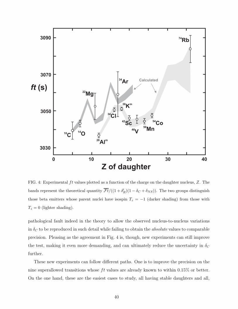
3030

3090

3050

10C

14O

26 mAl

34Cl

38 mK

42Sc

46V

50Mn

54Co

22Mg

74Rb

Calculated

403020100

Z of daughter

ft (s)

307034Ar

FIG. 4: Experimental ft values plotted as a function of the charge on the daughter nucleus, Z. The

bands represent the theoretical quantity Ft/((1 + δ′R)(1− δC + δNS)). The two groups distinguish

those beta emitters whose parent nuclei have isospin Tz = −1 (darker shading) from those with

Tz = 0 (lighter shading).

pathological fault indeed in the theory to allow the observed nucleus-to-nucleus variations

in δC to be reproduced in such detail while failing to obtain the absolute values to comparable

precision. Pleasing as the agreement in Fig. 4 is, though, new experiments can still improve

the test, making it even more demanding, and can ultimately reduce the uncertainty in δC

further.

These new experiments can follow different paths. One is to improve the precision on the

nine superallowed transitions whose ft values are already known to within 0.15% or better.

On the one hand, these are the easiest cases to study, all having stable daughters and all,

40

except 10C, decaying predominantly (> 99%) through a single superallowed transition. On

the other hand, they have been the subject of intense scrutiny for at least the past four

decades and, given the number of careful measurements already published, the prospects

for really significant improvements in these cases, at least in the near future, do not seem

bright. Nevertheless, a glance at Fig. 2 shows that some modest improvements are certainly

possible. If we accept as a goal that experiment should be a factor of two more precise than

theory, then we see that the QEC-values for10C, 14O, 26Alm, 42Sc and 46V, the half-lives of

10C, 26Alm, 42Sc and 50Mn, and the branching ratio for 10C can all bear improvement.

A second path is to expand the number of precisely measured superallowed emitters to

include cases for which the calculated nuclear-structure-dependent corrections are larger, or

show larger variations from nuclide to nuclide, than the values applied to the nine currently

best-known transitions. We argue that if the calculations reproduce the experimentally

observed variations where they are large, then that must surely verify their reliability for

the original nine transitions whose corrections are considerably smaller. The recent results

for 22Mg, 34Ar and 74Rb are the first cases of this type to reach sufficient precision that they

can contribute to the test (see Fig. 4) but more are sure to follow. We have included in our

survey all cases that we believe are potential candidates within the next few years.

Without doubt, these new cases present serious experimental challenges. In general, the

parent nuclei are more exotic and thus more difficult to produce in pure and statistically

useful quantities. They also exhibit more complex branching patterns, which for the cases

with A ≥ 62 include Gamow-Teller transitions that may be unobservable individually but

collectively can play a non-negligible role [81]. These heavier nuclei also have very short

half-lives, which currently limit the precision with which their QEC-values can be measured.

Even so, all these obstacles are obviously now being overcome and we may reasonably hope

that before long there will not only be more cases with precisely measured parameters, but

there will be more than one measurement of each parameter, an essential prerequisite for

reliable results at the level of precision needed to constrain the correction terms.

Although it would not impact significantly on the unitarity question, there is an additional

reason to improve the precision with which the ft values are known, particularly for the cases

with A ≤ 26. A scalar current, if it exists, would manifest itself as a 1/W -dependence in

the shape-correction function used in the f -value calculations (see Eq. (28)). Since the

superallowed transition energies decrease with A, this effect would be strongest for the

41

lightest nuclei, 10C and 14O. Improved precision in the Ft values for those two nuclei would

act directly to reduce the limits set on a possible scalar current.

In conclusion, we can assert that world data for superallowed 0+ → 0+ β decays strongly

support the CVC expectation of an unrenormalized vector coupling constant, and also set

a new limit on the possible existence of scalar currents. The nuclear-structure-dependent

corrections used in the analyses of these data have so far stood up very favorably to ex-

perimental tests, and the value currently obtained with them for Vud is deemed to be very

robust, even though it is an important component of the top-row test of CKM unitarity that

fails by more than two standard deviations. We have indicated the improvements required

from both theory and experiment to increase the precision in future so as to produce a more

definitive result for the unitarity test.

Acknowledgments

The work of JCH was supported by the U. S. Dept. of Energy under Grant DE-FG03-

93ER40773 and by the Robert A. Welch Foundation. IST would like to thank the Cyclotron

Institute of Texas A & M University for its hospitality during several two-month visits.

APPENDIX A: STATISTICAL RATE FUNCTION

The statistical rate function is an integral over phase space,

f =∫ W0

1pW (W0 −W )2F (Z,W )S(Z,W )dW, (A1)

where W is the electron total energy in electron rest-mass units, W0 is the maximum value

of W , p = (W 2 − 1)1/2 is the electron momentum, Z is the charge number of the daughter

nucleus (positive for electron emission, negative for positron emission), F (Z,W ) is the Fermi

function, and S(Z,W ) is the shape-correction function. If the shape-correction function is

put to unity, the integral becomes the customarily defined one for beta decay, which we will

denote as fstat:

fstat =∫ W0

1pW (W0 −W )2F (Z,W )dW. (A2)

The exact evaluation of f differs from fstat by 0.2% at A = 10 up to 5.7% at A = 74. Thus,

to maintain 0.1% accuracy for f over that range, we must determine the shape-correction

42

function itself with 2% accuracy. Obtaining this accuracy requires consideration of the

following issues:

• The electron wave functions can no longer be simply those of the lowest partial wave

(j = 1/2) generated by a point nuclear charge and evaluated at radius R, the nu-

clear surface, but must be the exact functions for some chosen nuclear charge-density

distribution;

• The lepton wavefunctions exhibit some r2 dependence over the nuclear volume, leading

to what are called second-forbidden corrections. Furthermore, a more accurate treat-

ment of the weak interaction leads to relativistic and induced-current corrections. All

these effects must be incorporated since they impact on the nuclear matrix elements

and inject a mild nuclear-structure dependence into the evaluation of f .

• The atomic electrons cannot be ignored, but must be accommodated approximately

in a screening correction;

In what follows we describe the ingredients of a code we have written that incorporates

these effects. It is based on the formalism of Behrens and Buhring [166]. Note that they

define

F (Z,W )S(Z,W ) = F0L0C(Z,W ), (A3)

where F0 = 2F (Z,W )/(1 + γ1). The purpose of their redefining the shape correction factor

in this way was to remove the historic requirement to evaluate the electron wave functions

at the nuclear surface. The product F0L0 is given entirely in terms of the amplitudes of

the electron wave function at the origin (see Eq. (A9) below), and C(Z,W ) is the shape-

correction function defined with respect to this choice.

1. Electron Radial Wave Functions

The wave function for the electron emitted in beta decay is given by the solution to

the Dirac equation with an external electromagnetic field present, but restricted to the

special case where the vector potential vanishes identically and the scalar potential is static

and spherically symmetric. We solve in spherical coordinates and introduce a partial wave

43

expansion such that the basis states are written:

ψµκ =

sign(κ)fκ(r)χµ–κ

gκ(r)χµκ

, (A4)

where fκ, gκ are radial functions, and χµκ are the usual spin-angular-momentum wave func-

tions describing the coupling of the orbital angular momentum l and spin 12 to give a total

angular momentum j with z-component µ:

χµκ = il

∑

mlms

〈lml12ms|jµ〉Ylml

(r)χms . (A5)

The eigenvalue κ is

κ = −j(j + 1) + l(l + 1)− 14 (A6)

and has values

κ = −(l + 1) = −(j + 12) if j = l + 1

2

κ = l = (j + 12) if j = l − 1

2 . (A7)

The radial functions are solutions to a pair of coupled equations

dgκdr

+(κ+ 1)

rgκ − (W + 1− V (r))fκ = 0

dfκdr

− (κ− 1)

rfκ + (W − 1− V (r))gκ = 0. (A8)

Here V (r) is a spherically symmetric static potential that represents the interaction of the

electron with the charge distribution of the nucleus.

Our task is to solve the pair of coupled radial equations, Eq. (A8), in three regions,

0 ≤ r ≤ R1, R1 ≤ r ≤ R2, R2 ≤ r ≤ ∞, matching the solutions at each region boundary.

The first region is the one over which the nuclear charge density is non-zero. Here, we

establish a power-series solution, regular at the origin, as the starting solution and integrate

numerically to R1. In the second region, we have a pure Coulomb potential, for which an

analytic solution can be found in terms of confluent hypergeometric functions of complex

argument. The asymptotic solution in the third region is expressed in terms of the desired

outgoing waves and a phase shift. The unknowns in the calculation are the phase shift, ∆κ,

and the normalization of the interior solution, ακ: they are determined from the matching

conditions.

44

In the derivation of expressions for beta-decay observables, certain combinations of am-

plitudes and phase shifts characterising the electron wave functions appear. These combi-

nations are called the beta-decay Coulomb functions, and are generally organized so that

they are of order unity, with corrections of order (αZ)2. Since we are only interested here in

the shape-correction function, the only such functions we need are F0L0, λk and µk, where

k = |κ|, which are defined as

F0L0 =α2–1 + α2

+1

2p2

λk =α2–k + α2

+k

α2–1 + α2

+1

µk =α2–k − α2

+k

α2–k + α2

+k

kW

γk, (A9)

where γk = {k2 − (αZ)2}1/2. Although these functions have actually been tabulated by

Behrens and Janecke [177], we have not used the tables but, in the interests of precision,

have explicitly computed the functions from the calculated values of ακ.

2. Shape-correction function

Behrens and Buhring [166] give the following expression for the shape-correction function:

C(Z,W ) =∑

kekνK

λke{

M2K(ke, kν) +m2

K(ke, kν)

−2µkeγkekeW

MK(ke, kν)mK(ke, kν)}

, (A10)

where the sums over ke and kν are partial-wave expansions of the electron and neutrino

wave functions with ke = je +12 and kν = jν +

12 , je and jν being the electron and neutrino

total angular momenta. The integer K represents the multipolarity of the transition oper-

ators and is limited to the range |je − jν | ≤ K ≤ je + jν . The functions MK(ke, kν) and

mK(ke, kν) are given in terms of form factors [166] and we evaluate these form factors in

the “impulse approximation”. In this approximation, the nucleus is treated as a collection

of non-interacting nucleons so it is only necessary to consider the weak interaction as acting

upon a single nucleon. All the many-body aspects of the nucleus can thus be handled in the

standard shell-model way. Let O be a one-body operator, which can be written

O =∑

αβ

〈α|O|β〉a†αaβ, (A11)

45

where a†α is the creation operator for a nucleon in quantum state α, and aβ is an annihilation

operator destroying a nucleon in state β. The matrix element of O for many-body states

becomes

〈f |O|i〉 =∑

αβ

〈α|O|β〉〈f |a†αaβ|i〉; (A12)

that is, the matrix element is a linear combination of single-particle matrix elements,

〈α|O|β〉. The coefficients in the expansion, 〈f |a†αaβ |i〉, are called one-body density matrix

elements (OBDME). We leave it, then, as the job of the shell model to provide the OBDMEs

and only deal here with the single-particle matrix elements. The functions MK(ke, kν) and

mK(ke, kν) are now given in terms of reduced nuclear matrix elements for a single-particle

transition jβ → jα by

MK(ke, kν) =

√4π

KJi

∑

Ls

(−)K−L〈jα || F (r)TKLs || jβ〉

mK(ke, kν) =

√4π

KJi

∑

Ls

(−)K−L〈jα || f(r)TKLs || jβ〉, (A13)

where is a short-hand notation for (2j + 1)1/2 and Ji is the spin of the decaying nucleus.

The radial functions are

F (r) = H(r) {G−− jkν−1(pνr)−G−+ jkν (pνr)}

+D(r) {G+− jkν−1(pνr)−G++ jkν(pνr)}

f(r) = h(r) {G−− jkν−1(pνr)−G−+ jkν (pνr)}

+d(r) {G+− jkν−1(pνr)−G++ jkν (pνr)} , (A14)

with

H(r) = 12 (fke(r) + g−ke(r))

D(r) = 12 (gke(r)− f−ke(r))

h(r) = 12 (fke(r)− g−ke(r))

d(r) = 12 (gke(r) + f−ke(r)) . (A15)

Here fκ(r) and gκ(r) are radial electron functions6, while the spherical Bessel functions

represent radial neutrino wave functions. The functions G++, G+−, G−+ and G−− are

6 The internal normalisations at the origin are here set to unity. Recall that these normalisations, ακ, have

been separated out into the beta-decay Coulomb functions, F0L0, (see Eq. (A9)).

46

short-hand notations for GKLs(ke, kν), GKLs(ke, –kν), GKLs( –ke, kν), and GKLs( –ke, –kν)

respectively, where the functions GKLs(κe, κν) contain all the angular momentum factors for

the leptons:

GKLs(κe, κν) = ilν+L+le(−)je−jν

sKeν lelν 〈le0 lν0|L0〉

K s L

je12 le

jν12 lν

. (A16)

Lastly, the operators TKLs depend on the angle and spin coordinates and are defined as

TMKLs(r) = (V0 + A0)i

LYLM(r)δK,L if s = 0

= (V +A).iLYKLM(r) if s = 1, (A17)

where V0, A0 are the time parts of the vector and axial-vector hadronic currents and V,

A are the space parts. Further YKLM(r) is a vector spherical harmonic [178], which in

Eq. (A17) forms a scalar product with vectors V and A.

3. Hadronic matrix element

For nucleons, the vector and axial-vector interactions are written

Vµ = gVγµ − fMσµνqν + ifSqµ

Aµ = gAγµγ5 − fTσµνqνγ5 + ifPqµγ5. (A18)

Were we discussing the weak interaction between point-like spin-1/2 fermions, then we would

set gV = gA = 1, and fM = fS = fT = fP = 0. However, in considering nucleons, we

recognize that they are not point-like and furthermore they are influenced by the presence

of the strong interaction. Thus Eq. (A18) presents the most general form of a vector and

axial-vector interaction that is consistent with Lorentz invariance and excludes momentum

operators beyond the first power. Here qµ = (pf − pi)µ is the momentum transfer. The

coefficients, in principle, could be functions of q2 but, because of the low four-momentum

transfer in beta decay, this q2 dependence can be neglected and the coefficients are referred

to as coupling constants with individual titles: gV being vector; gA, axial-vector; fM, weak

magnetic; fS, induced scalar; fT, induced tensor and fP, induced pseudoscalar.

47

Our aim is to reduce the matrix element iuf(Vµ+Aµ)ui, where uf and ui are Dirac spinors

characterising nucleons of momentum pf and pi, to the nonrelativistic form involving Pauli

two-component spinors,

χ†mf

(V0 +V + A0 +A)χmi, (A19)

by simply multiplying out the Dirac matrices involved and keeping terms to first order in

|p|/MN, and dropping terms in |p2|/M2Nand higher order. This multiplication yields

V0 = gV + fS(W0 − V (r)) (A20)

V =gV

2MN

[p+ iσ × q] + fMiσ × q− fSq (A21)

A0 = − gA

2MN

σ.p− fTσ.q (A22)

A = −gAσ + fT(W0 − V (r))σ, (A23)

where p = pf + pi and q = pf − pi. Note that the large terms of order unity occur in V0

and A. Each of the four coupling constants denoted by an f are small and of order 1/MN

and, as a consequence, terms in f/MN have been dropped. Eqs. (A20) to (A23) are the

quantities needed in the operators TMKLs(r) in Eq. (A17).

4. Reduced matrix elements

All the beta-decay observables [166] can be expressed in terms of the functionsMK(ke, kν)

and mK(ke, kν) defined in Eq. (A13). Here we are only interested in the shape-correction

function, Eq. (A10), which is a particularly simple combination of these quantities. Before

proceding to evaluate MK(ke, kν) and mK(ke, kν), we note that the expressions for both

differ only in the presence of F (r) in one case and f(r) in the other. For simplicity in what

follows, we will only explicitly display formulae incorporating f(r); obviously an equivalent

set can be written with F (r).

The operators TMKLs(r) are shown in Eq. (A17), but it is tidier if we incorporate the phase,

(−)K−L (see Eq. (A13)), into the operator. All the operators (some after rearrangement)

can then be expressed as a product of spherical tensors, one in orbital space and one in spin

space. So, generically the operators take the form

TMKLS(r) = f(r)(−)K−LTKM(ΛL ⊗ ΣS), (A24)

48

where ΛL is a spherical tensor in orbital space of multipolarity L, and ΣS a spherical tensor

in spin space7. We have introduced notation for a composite spherical tensor obtained from

the combination of two other spherical tensors: viz.

TKM(ΛL ⊗ ΣS) =∑

MLMS

〈LML SMS|KM〉ΛLMLΣSMS

. (A25)

The single-particle wave functions from the shell model can also be expressed as products

of orbital and spin space functions:

|jm〉 =∑

mlms

〈lml12ms|jm〉Rnl(r)i

lYlml(r)χms , (A26)

where n is the principal quantum number designating the number of nodes in the radial

function. Notice the presence of il with the spherical harmonics8.

The first step in evaluating the reduced matrix element is to factorize it into orbital and

spin reduced matrix elements:

〈(lα 12)jα || TKLS || (lβ 1

2)jβ〉 =

(−)K−LA(LS)K 〈lα || f(r)ΛL || lβ〉〈12 || ΣS || 12〉, (A27)

where

A(LS)K = αKβ

lα12 jα

lβ12 jβ

L S K

. (A28)

Our conventions on reduced matrix elements are those of Edmonds [178]. Next, we need to

define two spin matrix elements, denoted S0 and S1 and given by

S0 ≡ 〈12 || 1 || 12〉 =

√2 δS,0

S1 ≡ 〈12 || σ || 12〉 =

√6 δS,1; (A29)

and two two orbital matrix elements denoted LL and L(J1)L(Q). The first is

LL ≡ 〈lα || f(r)iLYL(r) || lβ〉

7 Note, the upper case S in Eq. (A24) referring to the multipolarity of the spin operator is not the same as

the lower case s in Eq. (A17).8 If one-body density matrix elements (OBDME) are imported from a shell-model calculation into this

beta-decay environment, then it is important that these OBDME be computed with similar il phases

included in the definition of single-particle wave functions.

49

= ilα+L+lβlαLlβ√4π

lα L lβ

0 0 0

〈Rα|f(r)|Rβ〉, (A30)

where the last factor is the radial integral:

〈Rα|f(r)|Rβ〉 ≡∫ ∞

0Rα(r)f(r)Rβ(r)r

2dr. (A31)

The second involves derivative operators and requires a little more care. The matrix element

is

L(J1)L(Q) ≡ 〈lα || f(r)iJTL(YJ ⊗Q) || lβ〉, (A32)

where Q is either p = pf+pi or q = pf−pi. Thus we write Q as pf±pi with the upper sign

appropriate for p and the lower sign for q. Now Q is also −i(∇f ±∇i), where the gradient

operator acts on either the initial or final nuclear wave function but not on the integrand,

f(r). Thus the interpretation is as follows: 〈φf |fQ|φi〉 = −i{±〈φf |f |∇φi〉 − 〈∇φf |f |φi〉}.The result for L(J1)L(Q) is

L(J1)L(Q) = ilα+lβ+J+1(−)J−L J√4π

×

{

±U(lβ1lαJ ; lβ + 1L)

lα J lβ + 1

0 0 0

lα(lβ + 1)1/2 〈 Rα|f | ( ddr −

lβr ) Rβ 〉

∓ U(lβ1lαJ ; lβ − 1L)

lα J lβ − 1

0 0 0

lα(lβ)1/2 〈 Rα|f | ( d

dr +lβ+1r ) Rβ 〉

− (−)J+1−LU(lβJlα1; lα + 1L)

lα + 1 J lβ

0 0 0

lβ(lα + 1)1/2 〈( ddr − lα

r ) Rα|f |Rβ 〉

+ (−)J+1−LU(lβJlα1; lα − 1L)

lα − 1 J lβ

0 0 0

lβ(lα)1/2 〈( d

dr +lα+1r ) Rα|f |Rβ 〉

}

,

(A33)

where the upper sign is used for Q = p and the lower sign for Q = q. The U -coefficient is

a recoupling of three angular momenta and is related to a 6j-symbol:

U(abcd; ef) = (−)a+b+c+d ef

a b e

d c f

. (A34)

50

Finally, we are ready to write down the specific reduced matrix elements for all the

different hadronic components of the weak interaction, Eqs. (A20) to (A23):

Time-like Vector Current

〈(lα 12)jα || f(r)V0iKYK || (lβ 1

2)jβ〉 =(

gV + fS

(

W0 +65αZR

))

A(K0)K LK S0. (A35)

Space-like Axial Current

〈(lα 12)jα || f(r)A.iLYKL || (lβ 1

2)jβ〉 = (−)K−L(

−gA + fT

(

W0 +65αZR

))

A(L1)K LL S1. (A36)

In Eqs. (A35) and (A36), for simplicity we have replaced the function, V (r) (see Eqs. (A20)

and (A23)) by the potential due to a uniform charge distribution for small r, with r2 replaced

by its expectation value. In our computations we actually included the function V (r) in the

integrand of the appropriate radial integral.

Space-like Vector Current

〈(lα 12)jα || f(r)V.iLYKL || (lβ 1

2)jβ〉 =

(−)K−L{

gV

2MN

A(K0)K L(L1)K(p) S0 − fSA(K0)K L(L1)K(q) S0

−√2∑

J

U(11KL; 1J)(

gV

2MN

+ fM

)

A(J1)K L(L1)J (q) S1

}

. (A37)

Time-like Axial Current

〈(lα 12)jα || f(r)A0i

KYK || (lβ 12)jβ〉 =

∑

J

(−)J−K J

K

{

− gA

2MN

A(J1)K L(K1)J (p) S1 − fTA(J1)K L(K1)J (q) S1

}

. (A38)

5. Numerical Results

The key ingredient for the computation of exact electron wave functions in beta decay is

the charge-density distribution of the daughter nucleus. There are various parameterizations

available in the literature, of which the following are the most common:

• Two-parameter Fermi distribution (2pF). This charge density distribution,

ρ(r) =ρ0

1 + exp{(r − c)/a} , (A39)

has two parameters, c and a, other than its normalization.

51

• Three-parameter Fermi distribution (3pF). This is an extension of the two-parameter

model, which introduces a dimensionless “wine-bottle” parameter, w, that impacts on

the small-r behaviour of the density distribution. The functional form is

ρ(r) =ρ0(1 + wr2/c2)

1 + exp{(r − c)/a} . (A40)

• Three-parameter Gaussian distribution (3pG). This is an alternative three-parameter

model with a Gaussian rather than a Fermi distribution:

ρ(r) =ρ0(1 + wr2/c2)

1 + exp{(r2 − c2)/a2} . (A41)

• Harmonic-oscillator distribution (HO). In light p-shell nuclei, where only s and p

orbitals are occupied, a density distribution can be constructed from the harmonic

oscillator radial wavefunctions. Its form is

ρ(r) = ρ0(1 + αr2/b2) exp(−r2/b2), (A42)

where b is the harmonic oscillator length parameter, and α is related to the number of

p-shell protons, α = (Z − 2)/3. However, in practise both b and α are treated as free

parameters and adjusted to fit the elastic-electron scattering data.

These model distributions typically contain two or three parameters. Where possible,

the parameters are determined from experimental data on elastic electron scattering, since

the measured electron-scattering form factors are just the Fourier transforms of the charge-

density distributions. A compilation of charge-density distributions determined from elec-

tron scattering is given by De Vries et al. [179]. We have assessed these data and selected

for each daughter nucleus what we believe to be the ‘best’ value of the rms radius, 〈r2〉1/2,and its probable error. In cases where data are not available on the isotope of interest, we

have examined the nearest isotope that is available and applied a modest isotope shift to its

value of 〈r2〉1/2. Our final selected values are listed in Table X. We also list the percentage

uncertainty in the exact value of f due solely to the uncertainty in 〈r2〉1/2. Clearly, the

uncertainty in the charge-density distribution is not a factor in the determination of f to

0.1% accuracy.

Before the final evaluation of the statistical rate function, f , there are two further cor-

rections to consider: for screening and recoil. To accommodate these corrections and to

52

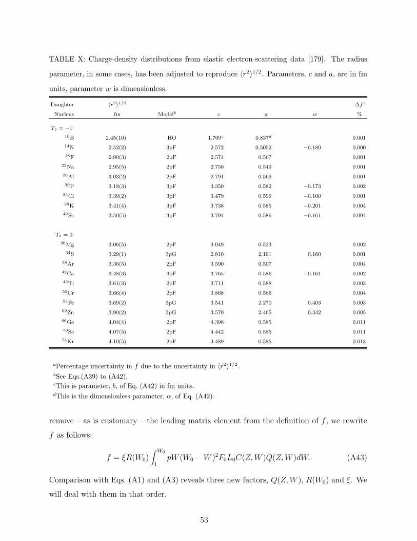
TABLE X: Charge-density distributions from elastic electron-scattering data [179]. The radius

parameter, in some cases, has been adjusted to reproduce 〈r2〉1/2. Parameters, c and a, are in fm

units, parameter w is dimensionless.

Daughter 〈r2〉1/2 ∆fa

Nucleus fm Modelb c a w %

Tz = −1:

10B 2.45(10) HO 1.709c 0.837d 0.001

14N 2.52(2) 3pF 2.572 0.5052 −0.180 0.000

18F 2.90(3) 2pF 2.574 0.567 0.001

22Na 2.95(5) 2pF 2.750 0.549 0.001

26Al 3.03(2) 2pF 2.791 0.569 0.001

30P 3.18(3) 3pF 3.350 0.582 −0.173 0.002

34Cl 3.39(2) 3pF 3.479 0.599 −0.100 0.001

38K 3.41(4) 3pF 3.738 0.585 −0.201 0.004

42Sc 3.50(5) 3pF 3.794 0.586 −0.161 0.004

Tz = 0:

26Mg 3.06(5) 2pF 3.049 0.523 0.002

34S 3.29(1) 3pG 2.810 2.191 0.160 0.001

38Ar 3.36(5) 2pF 3.590 0.507 0.004

42Ca 3.48(3) 3pF 3.765 0.586 −0.161 0.002

46Ti 3.61(3) 2pF 3.711 0.588 0.003

50Cr 3.66(4) 2pF 3.868 0.566 0.004

54Fe 3.69(2) 3pG 3.541 2.270 0.403 0.003

62Zn 3.90(2) 3pG 3.570 2.465 0.342 0.005

66Ge 4.04(4) 2pF 4.398 0.585 0.011

70Se 4.07(5) 2pF 4.442 0.585 0.011

74Kr 4.10(5) 2pF 4.489 0.585 0.013

aPercentage uncertainty in f due to the uncertainty in 〈r2〉1/2.bSee Eqs.(A39) to (A42).cThis is parameter, b, of Eq. (A42) in fm units.dThis is the dimensionless parameter, α, of Eq. (A42).

remove – as is customary – the leading matrix element from the definition of f , we rewrite

f as follows:

f = ξR(W0)∫ W0

1pW (W0 −W )2F0L0C(Z,W )Q(Z,W )dW. (A43)

Comparison with Eqs. (A1) and (A3) reveals three new factors, Q(Z,W ), R(W0) and ξ. We

will deal with them in that order.

53

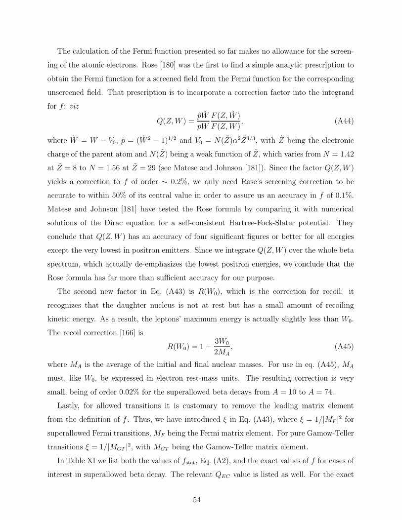
The calculation of the Fermi function presented so far makes no allowance for the screen-

ing of the atomic electrons. Rose [180] was the first to find a simple analytic prescription to

obtain the Fermi function for a screened field from the Fermi function for the corresponding

unscreened field. That prescription is to incorporate a correction factor into the integrand

for f : viz

Q(Z,W ) =pW

pW

F (Z, W )

F (Z,W ), (A44)

where W = W − V0, p = (W 2 − 1)1/2 and V0 = N(Z)α2Z4/3, with Z being the electronic

charge of the parent atom and N(Z) being a weak function of Z, which varies from N = 1.42

at Z = 8 to N = 1.56 at Z = 29 (see Matese and Johnson [181]). Since the factor Q(Z,W )

yields a correction to f of order ∼ 0.2%, we only need Rose’s screening correction to be

accurate to within 50% of its central value in order to assure us an accuracy in f of 0.1%.

Matese and Johnson [181] have tested the Rose formula by comparing it with numerical

solutions of the Dirac equation for a self-consistent Hartree-Fock-Slater potential. They

conclude that Q(Z,W ) has an accuracy of four significant figures or better for all energies

except the very lowest in positron emitters. Since we integrate Q(Z,W ) over the whole beta

spectrum, which actually de-emphasizes the lowest positron energies, we conclude that the

Rose formula has far more than sufficient accuracy for our purpose.

The second new factor in Eq. (A43) is R(W0), which is the correction for recoil: it

recognizes that the daughter nucleus is not at rest but has a small amount of recoiling

kinetic energy. As a result, the leptons’ maximum energy is actually slightly less than W0.

The recoil correction [166] is

R(W0) = 1− 3W0

2MA, (A45)

where MA is the average of the initial and final nuclear masses. For use in eq. (A45), MA

must, like W0, be expressed in electron rest-mass units. The resulting correction is very

small, being of order 0.02% for the superallowed beta decays from A = 10 to A = 74.

Lastly, for allowed transitions it is customary to remove the leading matrix element

from the definition of f . Thus, we have introduced ξ in Eq. (A43), where ξ = 1/|MF |2 for

superallowed Fermi transitions,MF being the Fermi matrix element. For pure Gamow-Teller

transitions ξ = 1/|MGT |2, with MGT being the Gamow-Teller matrix element.

In Table XI we list both the values of fstat, Eq. (A2), and the exact values of f for cases of

interest in superallowed beta decay. The relevant QEC value is listed as well. For the exact

54

TABLE XI: Comparison of statistical rate functions, fstat, fapprox and the exact value, f .

Parent QEC W0 fstat f ∆fstata

keV %

Tz = −1:

10C 1907.9 2.7336 2.29484 2.30089 −0.26

14O 2831.0 4.5400 42.6147 42.7485 −0.31

18Ne 3402.0 5.6575 133.867 134.484 −0.46

22Mg 4124.6 7.0716 415.826 418.440 −0.62

26Si 4836.9 8.4656 1014.75 1023.28 −0.83

30S 5459.5 9.6840 1945.49 1967.05 −1.10

34Ar 6062.8 10.8647 3366.22 3414.21 −1.41

38Ca 6614.2 11.9437 5247.54 5338.46 −1.70

42Ti 7000.9 12.7004 6904.47 7042.83 −1.96

Tz = 0:

26mAl 4232.5 7.2828 474.691 478.176 −0.73

34Cl 5491.8 9.7472 1971.95 1996.39 −1.22

38mK 6044.4 10.8286 3248.45 3298.10 −1.51

42Sc 6425.7 11.5748 4391.71 4470.41 −1.76

46V 7050.7 12.7979 7044.04 7199.96 −2.17

50Mn 7632.5 13.9364 10456.3 10731.6 −2.57

54Co 8242.7 15.1305 15281.4 15750.1 −2.98

62Ga 9171.0 16.9472 25187.9 26247.6 −4.04

66As 9550.0 17.6889 30146.4 31613.7 −4.64

70Br 9970.0 18.5108 36605.4 38602.2 −5.17

74Rb 10416.5 19.3846 44606.1 47277.8 −5.65

a∆fstat = 100 ∗ (fstat − f)/f

55

calculations, we imported one-body density matrix elements, OBDME, from a shell-model

code. For each case we performed several shell-model calculations for various sets of effective

interactions and model spaces. We used, in fact, the same wave functions that we used [158]

to compute the nuclear-structure corrections δC and δNS. Thus our f calculations can be

considered to be entirely consistent with the calculation of the nuclear-structure-dependent

corrections. The f calculation, however, is not very sensitive to the shell-model inputs. In

light nuclei, different shell-model OBDME gave changes in f at the 0.01% level, increasing to

around 0.1% in A = 74, our heaviest-mass case. Where we have more than one shell-model

calculation for a given nucleus, we have averaged the f values for the entry in Table XI.

[1] I.S. Towner and J.C. Hardy, J. Phys. G: Nucl. Part. Phys., 29, 197 (2003).

[2] A. Sher et al. , Phys. Rev. Lett. 91, 261802 (2003).

[3] I.S. Towner and J.C. Hardy, Nucl. Phys. A205, 33 (1973).

[4] J.C. Hardy and I.S. Towner, Nucl. Phys. A254, 221 (1975).

[5] V.T. Koslowsky, E. Hagberg, J.C. Hardy, H. Schmeing, R.E. Azuma and I.S. Towner, in

Proc. 7th Int. Conf. on atomic masses and fundamental constants, Darmstadt-Seeheim, ed.

O. Klepper (T.H. Darmstadt, 1984) p. 572

[6] J.C. Hardy, I.S. Towner, V.T. Koslowsky, E. Hagberg and H. Schmeing, Nucl. Phys. A509,

429 (1990).

[7] S. Eidelman et al, Phys. Lett. B592, 1 (2004).

[8] E.G. Adelberger, M.M. Hindi, C.D. Hoyle, H.E. Swanson, R.D. Von Lintig and W.C. Haxton,

Phys. Rev. C 27, 2833 (1983); this reference replaces the result reported in E.G. Adelberger,

C.D. Hoyle, H.E. Swanson and R.D. Von Lintig, Phys. Rev. Lett. 46, 695 (1981).

[9] F. Ajzenberg-Selove, Nucl. Phys. A490, 1 (1988).

[10] F. Ajzenberg-Selove, Nucl. Phys. A523, 1 (1991).

[11] A.M. Aldridge, K.W. Kemper and H.S. Plendl, Phys. Lett. 30B, 165 (1969)

[12] D.E. Alburger and D.H. Wilkinson, Phys. Let. 32B, 190 (1970).

[13] D.E. Alburger, Phys. Rev. C 5, 274 (1972).

[14] D.E. Alburger and F.P. Calaprice, Phys. Rev. C 12, 1690 (1975).

[15] D.E. Alburger and D.H. Wilkinson, Phys. Rev. C 15, 2174 (1977); this reference replaces the

56

46V half-life from [149].

[16] D.E. Alburger, Phys. Rev. C 18, 1875 (1978).

[17] P.F.A. Alkemade, C. Alderliesten, P. De Wit and C. Van der Leun, Nucl. Instr and Meth.

197, 383 (1982).

[18] A. Antilla, M. Bister and E. Arminen, Z. Phys. 234, 455 (1970).

[19] E. Aslanides, F. Jundt and A. Gallmann, Nucl. Phys. A152, 251 (1970).

[20] G. Audi, A.H. Wapstra and C. Thibault, Nucl. Phys. A729, 327 (2003).

[21] G. Azuelos, J.E. Crawford and J.E. Kitching, Phys. Rev. C 9, 1213 (1974).

[22] G. Azuelos and J.E. Kitching, Phys. Rev. C 12, 563 (1975).

[23] R.K. Barden, C.A. Barnes, W.A. Fowler and P.G. Seeger, Phys. Rev. 127, 583 (1962)

[24] F.J. Bartis, Phys. Rev. 132, 1763 (1963).

[25] P.H. Barker, N. Drysdale and W.R. Phillips, Proc. Phys. Soc 91, 587 (1967).

[26] P.H. Barker, C.J. Scofield, R.J. Petty, J.M. Freeman, S.D. Hoath, W.E. Burcham and G.T.A.

Squier, Nucl. Phys. A275, 37 (1977); the same result also appears in G.T.A. Squier, W.E.

Burcham, S.D. Hoath, J.M. Freeman, P.H. Barker and R.J. Petty, Phys. Lett. 65B, 122

(1976).

[27] P.H. Barker and J.A. Nolen, Proc. Int. Conf. on Nucl. Structure, Tokyo, Japan, 1977.

[28] P.H. Barker, R.E. White, H. Naylor and N.S. Wyatt, Nucl. Phys. A279, 199 (1977).

[29] P.H. Barker and R.E. White, Phys. Rev. C 29, 1530 (1984).

[30] P.H. Barker and S.M. Ferguson, Phys. Rev. C 38, 1936 (1988).

[31] S.C. Baker, M.J. Brown and P.H. Barker, Phys. Rev. C 40, 940 (1989).

[32] P.H. Barker and G.D. Leonard, Phys. Rev. C 41, 246 (1990).

[33] P.H. Barker and P.A. Amundsen, Phys. Rev. C58, 2571 (1998); this reference updates the

10C QEC-value from [31]; its value for the 14O QEC-value was later withdrawn in [141].

[34] P.H. Barker and M.S. Wu, Phys. Rev C 62, 054302 (2000).

[35] G.C. Ball, S. Bishop, J.A. Behr, G.C. Boisvert, P. Bricault, J. Cerny, J.M. D’Auria, M.

Dombsky, J.C. Hardy, V. Iacob, J.R. Leslie, T. Lindner, J.A. Macdonald, H.-B. Mak, D.M.

Moltz, J. Powell, G. Savard and I.S. Towner, Phys. Rev. Lett. 86, 1454 (2001).

[36] P.H. Barker, I.C. Barnett, G.J. Baxter and A.P. Byrne, Phys. Rev. C 70, 024302 (2004).

[37] G.C. Ball et al, to be published.

[38] E. Beck and H. Daniel, Z. Phys. 216, 229 (1968).

57

[39] J.A. Becker, R.A. Chalmers, B.A. Watson and D.H. Wilkinson, Nucl. Instr. Meth. 155, 211

(1978).

[40] F.J. Bergmeister, K.P. Lieb, K. Pampus and M. Uhrmacher, Z. Phys. A320, 693 (1985).

[41] S. Bishop et al., Phys. Rev. Lett. 90, 162501 (2003).

[42] B. Blank, Eur. Phys. J. A15, 121 (2002).

[43] B. Blank, G. Savard, J. Doring, A. Blazhev, G. Canchel, M. Chartier, D. Henderson, Z.

Janas, R. Kirchner, I. Mukha, E. Roeckl, K. Schmidt, and J. Zylicz, Phys. Rev. C 69,

015502 (2004).

[44] K. Blaum, G. Audi, D. Beck, G. Bollen, C. Guenaut, P. Delahaye, F. Herfurth, A. Keller-

bauer, H.-J. Kluge, D. Lunney, D. Rodriguez, S. Schwarz, L. Schweikhard, C. Weber and C.

Yazidjian, Nucl. Phys. A, to be published.

[45] R.O. Bondelid and J.W. Butler, Nucl. Phys. 53, 618 (1964).

[46] S.A. Brindhaban and P.H. Barker, Phys. Rev. C 49, 2401 (1994); reference replaces earlier

conference proceedings from the same laboratory.

[47] J.W. Butler and R.O. Bondelid, Phys. Rev. 121, 1770 (1961).

[48] W.E. Burcham and G.T.A. Squier, Nucl. Instr. And Meth. 164, 533 (1979).

[49] R.H. Burch, C.A. Gagliardi and R.E. Tribble, Phys. Rev. C 38, 1365 (1988).

[50] G. Canchel, B. Blank, M. Chartier, F. Delalee, P. Dendooven, C. Dossat, J. Giovinazzo, J.

Huikari, A.S. Lalleman, M.J. Lopez Jimenez, V. Madec, J.L. Pedroza, H. Penttila and J.C.

Thomas, Eur. Phys. J. A, to be published.

[51] N.M. Chaudri, Fizika 16, 297 (1984).

[52] G.J. Clark, J.M. Freeman, D.C. Robinson, J.S. Ryder, W.E. Burcham and G.T.A. Squier,

Nucl. Phys. A215, 429 (1973); this reference replaces the half-life value in G.J. Clark, J.M.

Freeman, D.C. Robinson, J.S. Ryder, W.E. Burcham and G.T.A. Squier, Phys. Lett 35B,

503 (1971).

[53] C.N. Davids, C.A. Gagliardi, M.J. Murphy and E.B. Norman, Phys. Rev. C 19, 1463 (1979).

[54] C.N. Davids, in “Atomic masses and fundamental constants 6”, eds. J.A. Nolen and W.

Benenson (Plenum, New York, 1980) p. 419.

[55] W.W. Daehnick and R.D. Rosa, Phys. Rev. C 31, 1499 (1985).

[56] P. De Wit and C. Van der Leun, Phys. Lett. 30B, 639 (1969).

[57] R.M. DelVecchio and W.W. Daehnick, Phys. Rev. C 17, 1809 (1978).

58

[58] M.A. van Driel, H. Klijnman, G.A.P. Engelbertink, H.H. Eggebhuisen and J.A.J. Hermans,

Nucl. Phys. A240, 98 (1975).

[59] L.G. Earwaker, J.G. Jenkin and E.W. Titterton, Nature 195, 271 (1962).

[60] P.M. Endt, Nucl. Phys. A521, 1 (1990).

[61] P.M. Endt, Nucl. Phys. A633, 1 (1998).

[62] G. Frick, A. Gallmann, D.E. Alburger, D.H. Wilkinson and J.P. Coffin, Phys. Rev. 132, 2169

(1963).

[63] J.M. Freeman, G. Murray and W.E. Burcham, Phys.Lett. 17, 317 (1965).

[64] J.M. Freeman, J.G. Jenkin, G. Murray, D.C. Robinson and W.E. Burcham, Nucl. Phys.

A132, 593 (1969); this reference replaces the half-life values in J.M. Freeman, J.H. Montague,

G. Murray, R.E. White and W.E. Burcham, Nucl. Phys. 69, 433 (1965) and J.M. Freeman,

J.G. Jenkin, G. Murray and W.E. Burcham, Phys. Rev. Lett. 16, 959 (1966).

[65] J.M. Freeman, R.J. Petty, S.D. Hoath, G.T.A. Squier and W.E. Burcham, Phys. Lett 53B,

439 (1975).

[66] B.K. Fujikawa, S.J. Asztalos, R.M. Clark, M.A. Deleplanque-Stephens, P. Fallon, S.J. Free-

man, J.P. Greene, I.-Y. Lee, L.J. Lising, A.O. Macchiavelli, R.W. MacLeod, J.C. Reich, M.A.

Rowe, S.-Q. Shang, F.S. Stephens and E.G. Wasserman, Phys. Lett. B449, 6 (1999).

[67] A Gallmann, E. Aslanides, F. Jundt and E. Jacobs, Phys. Rev. 186, 1160 (1969).

[68] M. Gaelens, J. Andrzejewski, J. Camps, P. Decrock, M. Huyse, K. Kruglov, W.F. Mueller,

A. Piechaczek, N. Severijns, J. Szerypo, G. Vancraeynest, P. Van Duppen and J. Wauters,

Eur. Phys. J. A11, 413 (2001).

[69] H.J. Gils, D. Flothmann, R. Loehken and W. Wiesner, Nucl. Instr. and Meth. 105, 179

(1972).

[70] D.R. Goosman and D.E. Alburger, Phys. Rev. C 5, 1893 (1972); the branching-ratio upper

limit set in this reference is considered to replace the much higher value reported by D.R.

Brown, S.M. Ferguson and D.H. Wilkinson, Nucl. Phys. A135, 159 (1969).

[71] G.I. Harris and A.K. Hyder, Phys. Rev. 157, 958 (1967).

[72] M. Hagen, K.H. Maier and R. Michaelsen, Phys. Lett. 26B, 432 (1968).

[73] J.C. Hardy and D.E. Alburger, Phys. Lett. B42, 341 (1972).

[74] J.C. Hardy, H. Schmeing, J.S. Geiger and R.L. Graham, Nucl. Phys. A223, 157 (1974); this

reference replaces results in J.C. Hardy, H. Schmeing, J.S. Geiger, R.L. Graham and I.S.

59

Towner, Phys. Rev. Lett. 29, 1027 (1972).

[75] J.C. Hardy, H.R. Andrews, J.S. Geiger, R.L. Graham, J.A. Macdonald and H. Schmeing,

Phys. Rev. Lett. 33, 1647 (1974).

[76] J.C. Hardy, H. Schmeing, W. Benenson, G.M. Crawley, E. Kashy and H. Nann, Phys. Rev.

C 9, 252 (1974).

[77] J.C. Hardy, G.C. Ball, J.S. Geiger, R.L. Graham, J.A. Macdonald and H. Schmeing, Phys.

Rev. Lett. 33, 320 (1974); the value for the 46V QEC-value from this reference was later

withdrawn by J.C. Hardy and I.S. Towner, in “Atomic masses and fundamental constants

5”, eds. J.H. Sanders and A.H. Wapstra (Plenum, New York, 1976) p 66.

[78] J.C. Hardy, H Schmeing, J.S. Geiger and R.L. Graham, Nucl. Phys. A246, 61 (1975); this

reference replaces results in J.C. Hardy, H. Schmeing, J.S. Geiger, R.L. Graham and I.S.

Towner, Phys. Rev. Lett. 29, 1027 (1972).

[79] E. Hagberg, V.T. Koslowsky, J.C. Hardy, I.S. Towner, J.G. Hykawy, G. Savard and T. Shi-

nozuka, Phys. Rev. Lett. 73, 396 (1994); uncertainties on the Gamow-Teller decays observed

from 46V and 50Mn did not appear in this reference but have been derived from the original

data and added here.

[80] P.D. Harty, N.S. Bowden, P.H. Barker and P.A. Amundsen, Phys. Rev. C 58, 821 (1998).

[81] J.C. Hardy and I.S. Towner, Phys. Rev. Lett. 88, 252501 (2002).

[82] J.C. Hardy, V.E. Iacob, M. Sanchez-Vega, R.G. Neilson, A Azhari, C.A. Gagliardi, V.E.

Mayes, X. Tang, L. Trache and R.E. Tribble, Phys. Rev. Lett. 91, 082501 (2003).

[83] D.L. Hendrie and J.B. Gerhart, Phys. Rev. 121, 846 (1961).

[84] A.M. Hernandez and W.W. Daehnick, Phys. Rev. C 24, 2235 (1981).

[85] A.M. Hernandez and W.W. Daehnick, Phys. Rev. C 25, 2957 (1982).

[86] F. Herfurth et al, Eur. Phys. J. A15, 17 (2002).

[87] I. Hofmann, Acta Phys. Aust. 18, 309 (1964).

[88] S.D. Hoath, R.J. Petty, J.M. Freeman, G.T.A. Squier and W.E. Burcham, Phys. Lett. 51B,

345 (1974).

[89] P. Hungerford and H.H. Schmidt, Nucl. Instr. and Meth. 192, 609 (1982).

[90] B.C. Hyman, V.E. Iacob, A. Azhari, C.A. Gagliardi, J.C. Hardy, V.E. Mayes, R.G. Neilson,

M. Sanchez-Vega, X. Tang, L. Trache and R.E. Tribble, Phys. Rev. C 68, 015501 (2003).

[91] V.E. Iacob, E. Mayes, J.C. Hardy, R.G. Neilson, M. Sanchez-Vega, A. Azhari, C.A. Gagliardi,

60

L. Trache and R.E. Tribble, Bul. Am. Phys. Soc. 48, 34 (2003).

[92] P.D. Ingalls, J.C. Overley and H.S. Wilson, Nucl. Phys. A293, 117 (1977).

[93] M.A. Islam, T.J. Kennett, S.A. Kerr and W.V. Prestwich, Can. J. Phys. 58, 168 (1980).

[94] J. Jaenecke, Z. Naturf. 15a, 593 (1960).

[95] A.N. James, F.J. Sharpey-Schafer, A.M. Al-Naser, A.H. Behbehani, C.J. Lister, P.J. Nolan,

P.H. Barker and W.E. Burcham, J. Phys. G 4, 579 (1978).

[96] R.W. Kavanagh, A. Gallmann, E. Aslanides, F. Jundt and E. Jacobs, Phys. Rev. 175, 1426

(1968).

[97] R.W. Kavanagh, Nucl. Phys A129, 172 (1969).

[98] A. Kellerbauer, G. Audi, D. Beck, K. Blaum, G. Bollen, B.A. Brown, P. Delahaye, C. Gue-

naut, F. Herfurth, H.-J. Kluge, D. Lunney, S. Schwarz, L. Schweikhard and C. Yazidjian,

Phys. Rev. Lett., 93, 072502 (2004).

[99] S.W. Kikstra, C. van der Leun, S. Raman, E.T. Jurney and I.S. Towner, Nucl. Phys. A496,

429 (1989).

[100] S.W. Kikstra, Z. Guo, C. Van der Leun, P.M. Endt, S. Raman, Walkiewicz, J.W. Starner,

E.T. Jurney and I.S. Towner, Nucl. Phys. A529, 39 (1991).

[101] V.T. Koslowsky, E. Hagberg, J.C. Hardy, R.E. Azuma, E.T.H. Clifford, H.C. Evans, H.

Schmeing, U.J. Schrewe and K.S. Sharma, Nucl. Phys. A405, 29 (1983).

[102] V.T. Koslowsky, J.C. Hardy, E. Hagberg, R.E. Azuma, G.C. Ball, E.T.H. Clifford, W.G.

Davies, H. Schmeing, U.J. Schrewe and K.S. Sharma, Nucl. Phys. A472, 419 (1987); the

14O-26Alm QEC-value-difference result reported in this reference replaces an earlier value

given in V.T. Koslowsky, J.C. Hardy, R.E. Azuma, G.C. Ball, E.T.H. Clifford, W.G. Davies,

E. Hagberg, H. Schmeing, U.J. Schrewe and K.S. Sharma, Phys. Lett. 119B, 57 (1982).

[103] V.T. Koslowsky, E. Hagberg, J.C. Hardy, G. Savard, H. Schmeing, K.S. Sharma and X.J.

Sun, Nucl.Instr.and Meth. A401, 289 (1997).

[104] V.T. Koslowsky, E. Hagberg, J.C. Hardy, H. Schmeing and I.S. Towner, Nucl. Phys. A624,

293 (1997).

[105] M.A. Kroupa, S.J. Freeman, P.H. Barker and S.M. Ferguson, Nucl. Instr. And Meth. in Phys.

Res. A310, 649 (1991).

[106] S. Lin, S.A. Brindhaban and P.H. Barker, Phys. Rev. C 49, 3098 (1994).

[107] P.V. Magnus, E.G. Adelberger and A. Garcia, Phys. Rev. C 49, R1755 (1994).

61

[108] W.R. McMurray, P. Van der Merwe and I.J. Van Heerden, Nucl. Phys. A92, 401 (1967).

[109] R.G. Miller and R.W. Kavanagh, Nucl. Phys. A94, 261 (1967).

[110] C.E. Moss, C. Detraz and C.S. Zaidins, Nucl. Phys. A174, 408 (1971).

[111] M. Mukherjee, A. Kellerbauer, D. Beck, K. Blaum, G. Bollen, F. Carrel, P. Delahaye, J.

Dilling, S. George, C. Guenaut, F. Herfurth, A. Herlert, H.-J. Kluge, U. Koster, D. Lunney,

S. Schwarz, L. Schweikhard and C. Yazidjian, Phys. Rev. Lett. 93, 150801 (2004).

[112] Y. Nagai, K. Kunihiro, T. Toriyama, S. Harada, Y. Torii, A. Yoshida, T. Nomura, J. Tanaka

and T. Shinozuka, Phys. Rev. C 43, R9 (1991).

[113] F.M. Nichols, N. Lawley, I.G. Main, M.F. Thomas and P.J. Twin, Nucl. Phys. A124, 97

(1969).

[114] J.A. Nolen, G. Hamilton, E. Kashy and I.D. Proctor, Nucl. Instr. and Meth. 115, 189 (1974).

[115] M.Oinonen et al, Phys. Lett. B511, 145 (2001).

[116] R.A. Padock, Phys. Rev. C 5, 485 (1972).

[117] A. Piechaczek, E.F. Zganjar, G.C. Ball, P. Bricault, J.M. D’Auria, J.C. Hardy, D.F. Hodg-

son, V. Iacob, P Klages, W.D. Kulp, J.R. Leslie, M. Lipoglavsek, J.A. Macdonald, H.-B.

Mak, D.M. Moltz, G. Savard, J. von Schwarzenberg, C.E. Svensson, I.S. Towner and J.L.

Wood, Phys. Rev. C 67, 051305(R) (2003); the branching-raio results from this measure-

ment are considered to replace the contradictory upper limit set in an earlier less-precise

measurement[115].

[118] F.W. Prosser, G.U. Din and D.D. Tolbert, Phys. Rev. 157, 779 (1967).

[119] W.V. Prestwich and T.J. Kennett, Can. J. Phys. 68, 261 (1990); erratum 68, 1352 (1990).

[120] S. Raman, E.T. Jurney, D.A. Outlaw and I.S. Towner, Phys. Rev. C 27, 1188 (1983).

[121] J.P.L. Reinecke, F.B. Waanders, P. Oberholtzer, P.J.C. Janse van Rensburg, J.A. Cilliers,

J.J.A. Smit, M.A. Meyer and P.M. Endt, Nucl. Phys. A435, 333 (1985).

[122] M.L. Roush, L.A. West and J.B. Marion, Nucl. Phys. A147, 235 (1970).

[123] D.C. Robinson, J.M. Freeman and T.T. Thwaites, Nucl. Phys. A181, 645 (1972); this refer-

ence replaces the 10C branching ratio from J.M. Freeman, J.G. Jenkin and G. Murray, Nucl.

Phys. A124, 393 (1969).

[124] D.C. Robinson and P.H. Barker, Nucl. Phys. A225, 109 (1974).

[125] C. Rolfs, W.S. Rodney, S. Durrance and H. Winkler, Nucl. Phys. A240, 221 (1975).

[126] J.S. Ryder, G.J. Clark, J.E. Draper, J.M. Freeman, W.E. Burcham and G.T.A. Squier, Phys.

62

Lett 43B, 30 (1973).

[127] A Rytz, At. Data and Nucl. Data Tables 47, 205 (1991).

[128] A.M. Sandorfi, C.J. Lister, D.E. Alburger and E.K. Warburton, Phys. Rev. C 22, 2213

(1980).

[129] G. Savard, A. Galindo-Uribarri, E. Hagberg, J.C. Hardy, V.T. Koslowsky, D.C. Radford and

I.S. Towner, Phys. Rev. Lett. 74, 1521 (1995).

[130] G. Savard, J.A. Clark, F. Buchinger, J.E. Crawford, S. Gulick, J.C. Hardy, A.A. Hecht, V.E.

Iacob, J.K.P. Lee, A.F. Levand, B.F. Lundgren, N.D. Scielzo, K.S. Sharma, I. Tanihata, I.S.

Towner, W. Trimble, J.C. Wang, Y. Wang and Z. Zhou, Phys. Rev. C 70, 042501(R) (2004).

[131] R.J. Scott, R.P. Rassool, M.N. Thompson and D.V. Webb, Nucl. Instr. and Meth. in Phys.

Res. A, to be published.

[132] J.C. Sens, A. Pape and R. Armbruster, Nucl. Phys. A199, 241 (1973).

[133] K.K. Seth, A. Saha, W. Benenson, W.A. Lanford, H. Nann and B.H. Wildenthal, Phys. Rev.

Lett. 33, 233 (1974).

[134] D. Seweryniak, to be published.

[135] R. Sherr, J.B. Gerhart, H. Horie and W.F. Hornyak, Phys. Rev. 100, 945 (1955).

[136] G.S. Sidhu and J.B. Gerhart, Phys. Rev. 148, 1024 (1963).

[137] J. Singh, Indian J. Pure Appl. Phys. 10, 289 (1972).

[138] G.T.A. Squier, W.E. Burcham, J.M. Freeman, R.J. Petty, S.D. Hoath and J.S. Ryder, Nucl.

Phys A242, 62 (1975).

[139] G.T.A. Squier, W.E. Burcham, S.D. Hoath, J.M. Freeman, P.H. Barker and R.J. Petty, Phys.

Lett. 65B, 122 (1976).

[140] D.R. Tilley, H.R. Weller, C.M. Cheves and R.M. Chasteler, Nucl. Phys. A595, 1 (1995).

[141] N.R. Tolich, P.H. Barker, P.D. Harty and P.A. Amundsen, Phys. Rev. C 67, 035503 (2003).

[142] H. Vonach, P. Glaessel, E. Huenges, P. Maier-Komor, H. Roesler, H.J. Scheerer, H. Paul and

D. Semrad, Nucl. Phys. A278, 189 (1977).

[143] F.B. Waanders, J.P.L. Reinecke, H.N. Jacobs, J.J.A. Smit, M.A. Meyer and P.M. Endt, Nucl.

Phys. A411, 81 (1983).

[144] T.A. Walkiewicz, S. Raman, E.T. Jurney, J.W. Starner and J.E. Lynn, Phys. Rev. C 45,

1597 (1992).

[145] H. Wenninger, J. Stiewe and H. Leutz, Nucl. Phys. A109, 561 (1968).

63

[146] R.E. White and H. Naylor, Nucl. Phys. A276, 333 (1977).

[147] R.E. White, H. Naylor, P.H. Barker, D.M.J. Lovelock and R.M. Smythe, Phys. Lett. 105B,

116 (1981).

[148] R.E. White, P.H. Barker and D.M.J. Lovelock, Metrologea 21, 193 (1985).

[149] D.H. Wilkinson and D.E. Alburger, Phys. Rev. C 13, 2517 (1976).

[150] D.H. Wilkinson, A. Gallmann and D.E. Alburger, Phys. Rev. C 18, 401 (1978).

[151] H.S. Wilson, R.W. Kavanagh and F.M. Mann, Phys. Rev. C 22, 1696 (1980).

[152] J. Zioni, A.A. Jaffe, E. Friedman, N. Haik, R. Schectman and D. Nir, Nucl. Phys. A181,

465 (1972).

[153] F. Zijderhand, R.C. Markus and C. van der Leun, Nucl. Phys. A466, 280 (1987).

[154] W. Bambynek, H. Behrens, M.H. Chen, B. Crasemann, M.L. Fitzpatrick, K.W.D. Leding-

ham, H. Genz, M. Mutterer and R.L. Intemann, Rev. Mod. Phys. 49, 77 (1977).

[155] R.B. Firestone, Table of Isotopes, Eighth Edition, (Wiley, New York, 1996).

[156] A. Sirlin, Phys. Rev. D 35, 3423 (1987); A. Sirlin and R. Zucchini, Phys. Rev. Lett. 57, 1994

(1986).

[157] W. Jaus and G. Rasche, Phys. Rev. D 35, 3420 (1987).

[158] I.S. Towner and J.C. Hardy, Phys. Rev. C 66, 035501 (2002).

[159] W.E. Ormand and B.A. Brown, Phys. Rev. C 52, 2455 (1995); W.E. Ormand and B.A.

Brown, Phys. Rev. Lett. 62, 866 (1989); W.E. Ormand and B.A. Brown, Nucl. Phys. A440,

274 (1985).

[160] H. Sagawa, N. Van Giai and T. Suzuki, Phys. Rev. C 53, 2163 (1996).

[161] F.C. Barker, Nucl. Phys. A537, 134 (1992).

[162] D.H. Wilkinson, Nucl. Instr. and Meth. A 488, 654 (2002); D.H. Wilkinson, Nucl. Instr. and

Meth. A 526, 386 (2004).

[163] W.J. Marciano and A. Sirlin, Phys. Rev. Lett. 56, 22 (1986).

[164] A. Sirlin, in Precision Tests of the Standard Electroweak Model, edited by P. Langacker

(World-Scientific, Singapore, 1994).

[165] J.D. Jackson, S.B. Treiman and H.W. Wyld Jr., Phys. Rev. 106, 517 (1957).

[166] H. Behrens and W. Buhring, Electron Radial Wave Functions and Nuclear Beta-decay

(Clarendon Press, Oxford, 1982).

[167] S. Weinberg, Phys. Rev. 112, 1375 (1958).

64

[168] B.R. Holstein, Phys. Rev. C 29, 623 (1984).

[169] P. Herczeg, Phys. Rev. D 34, 3449 (1986).

[170] P. Herczeg, Prog. Part. Nucl. Phys., 46, 413 (2001).

[171] M.A.B. Beg, R.V. Budny, R. Mohapatra and A. Sirlin, Phys. Rev. Lett. 38, 1252 (1977).

[172] J. Erler and M.J. Ramsey-Musolf, arXiv:hep-ph/0404291.

[173] A. Sirlin, Rev. Mod. Phys. 50, 573 (1978).

[174] I.S. Towner, Nucl. Phys. A540, 478 (1992).

[175] I.S. Towner, Phys. Lett. B333, 13 (1994).

[176] S. Ando, H.W. Fearing, V. Gudkov, K. Kubodera, F. Myhrer, S. Nakamura and T. Sato,

Phys. Lett. B595, 250 (2004).

[177] H. Behrens and J. Janecke, Numerical Tables for Beta Decay and Electron Capture, Landolt-

Bornstein, New Series I/4 (Springer-Verlag, Berlin, 1969).

[178] A.R. Edmonds, Angular Momentum in Quantum Mechanics, (Princeton University Press,

1964).

[179] H. De Vries, C.W. De Jager and C. De Vries, Atomic Data and Nucl. Data Tables 36, 495

(1987).

[180] M.E. Rose, Phys. Rev. 49, 727 (1936).

[181] J.J. Matese and W.R. Johnson, Phys. Rev. 150, 846 (1966).

65