arX

iv:a

stro

-ph/

0010

039v

5 2

7 Se

p 20

01Preprint UBC-COS-00-05, astro-ph/0010039

Power spectrum normalization from the local abundance of

rich clusters of galaxies

Elena Pierpaoli1, Douglas Scott1 and Martin White21Department of Physics and Astronomy, University of British Columbia, BC V6T1Z1 Canada2Harvard-Smithsonian Center for Astrophysics, Cambridge, MA 02138

Accepted ... ; Received ... ; in original form ...

ABSTRACT

The number density of rich galaxy clusters still provides the most robust way of normal-izing the power spectrum of dark matter perturbations on scales relevant to large-scalestructure. We revisit this constraint in light of several recent developments: (1) theavailability of well-defined samples of local clusters with relatively accurate X-ray tem-peratures; (2) new theoretical mass functions for dark matter haloes which provide agood fit to large numerical simulations; (3) more accurate mass-temperature relationsfrom larger catalogues of hydrodynamical simulations; (4) the requirement to considerclosed as well as open and flat cosmologies to obtain full multi-parameter likelihoodconstraints for CMB and SNe studies. We present a new sample of clusters drawn fromthe literature and use this sample to obtain improved results on σ8, the normalizationof the matter power spectrum on scales of 8 h−1Mpc, as a function of the matter den-sity and cosmological constant in a Universe with general curvature. We discuss ourdifferences with previous work, and the remaining major sources of uncertainty. Finalresults on the normalization, approximately independent of power spectrum shape, canbe expressed as constraints on σ at an appropriate cluster normalization scale RCl. Weprovide fitting formulas for RCl and σ(RCl) for general cosmologies, as well as for σ8 asa function of cosmology and shape parameter Γ. For flat models we find approximatelyσ8 ≃ (0.495+0.034

−0.037)Ω−0.60

Mfor Γ = 0.23, where the error bar is dominated by uncertainty

in the mass-temperature relation.

Key words: cosmology: theory – large-scale structure of Universe – galaxies: clusters– X-rays

1 INTRODUCTION

In theories of hierarchical structure formation the class ofobjects most recently formed holds a special significance.Observationally this class of objects is clusters of galaxies –the largest virialized structures in the present day universe.The local abundance of rich clusters of galaxies provides astrong constraint on the fluctuations in the matter densityon scales of order 10Mpc (Evrard 1989; Frenk et al. 1990;Bond & Myers 1991; Henry & Arnaud 1991; Kaiser 1991;Lilje 1992; Oukbir & Blanchard 1992; Bahcall & Cen 1993;Hanami 1993; White, Efstathiou & Frenk 1993). Consistencywith this constraint is one of the most important tests amodel can pass, since the constraint is directly on the lineartheory power spectrum, at a scale where there is an abun-dance of data. By fixing the normalization at wavelengthsmuch smaller than those probed by COBE one obtains anaccurate local normalization on scales relevant to much ofstructure formation, a long lever arm for constraining the

shape of the power spectrum, and a normalization to mat-ter fluctuations which is independent of galaxy bias.

There have been several recent and detailed studies ofthe cluster abundance, including Bond & Myers (1996), Eke,Cole & Frenk (1996), Viana & Liddle (1996; 1999), Co-lafrancesco, Mazzotta & Vittorio (1997), Kitayama & Suto(1997), Eke et al. (1998), Pen (1998), Wang & Steinhardt(1998), Donahue & Voit (1999) and Henry (2000). However,even more recently, there have been several developmentsin terms of both theory and observation which suggest itwould be useful to revisit this constraint. Firstly the addi-tion of ASCA temperatures (Tanaka, Inoue & Holt 1994)means that there is now a well defined local temperaturefunction for clusters, with relatively small errors in temper-ature. Secondly a number of large N-body simulations haveaccurately determined the mass function of virialized haloes(e.g. Governato et al. 1999), finding non-negligible devia-tions from the old Press-Schechter (1974; hereafter PS) the-ory. For example the extremely large N-body simulationsof the Virgo consortium have highlighted systematic depar-

2 E. Pierpaoli, D. Scott & M. White

tures from the PS predicted mass functions (Jenkins et al.2001), which alter the constraints on the power spectrumnormalization coming from the cluster abundance. Thirdly,more ambitious hydrodynamical simulations of cluster for-mation (e.g. Frenk et al. 1999, and references therein) haveresulted in improvements in the relationship between massand temperature and a better estimate of its scatter. Finally,the increased sophistication of multi-parameter cosmologi-cal studies (in particular driven by recent CMB anisotropymeasurements) requires that cosmological models with gen-eral curvature be considered (see e.g. White & Scott 1996).

With these refinements our results are an improvementover other studies of the past few years. We point out ex-plicitly where we differ from other work, and also where wethink things could be further improved in the future. Theoutline of the paper is as follows: we review some of theappropriate theory in §2; our local sample of clusters is pre-sented in §3; we describe our statistical method in §4; andwe present our results and conclusions in §5 and §6.

2 THEORY

The abundance of rich clusters is tied to the normalization ofthe power spectrum (extrapolated to the present using lin-ear theory) through the Press-Schechter (1974) theory andits extensions (see Sheth, Mo & Tormen 2000 and referencestherein). The theory has always had a somewhat weak ana-lytic justification, its widespread adoption arising from thedual facts that it is easy to use and provides a remarkablygood fit to more computationally expensive simulations.

Although galaxy velocity dispersion and gravitationallensing mass estimates exist for many clusters (Carlberg etal. 1996; Smail et al. 1997; Girardi et al. 1998a; Allen 1998;Wu et al. 1998; Girardi et al. 2000), the direct estimationof mass through determination of the X-ray temperature isfar more reliable – although the situation is certainly im-proving, allowing for estimates of the mass function (Gi-rardi et al. 1998b; Borgani et al. 1999). In the X-ray bandthere is considerably more high quality data on luminos-ity than on temperature, but there is enormous uncertaintyin deriving mass M from luminosity LX. Hence our pointof comparison between theory and observation will be thetemperature function of rich clusters, i.e. the number den-sity of clusters within a temperature range dT about T . Thisneeds to be observationally determined over some range of Tsufficiently high that gravitational physics dominates. Ob-servational and theoretical considerations place this limitat TX >∼ 3.5 keV (e.g. Finoguenov et al. 2000; Nevalainen,Markevitch & Forman 2000). Ideally we could compare thedata with a temperature function estimated directly from aseries of large cosmological hydrodynamic simulations (seee.g. Pen 1998), which included all of the physics relevantto determining the emission weighted inter-galactic medium(IGM) temperature of clusters. This however is currentlycomputationally infeasible. Instead we shall make use of thefact that rich clusters are large virialized structures domi-nated by gravity, and thus we can factorize the problem andproceed in two steps.

First we shall use the abundance of dark matter haloesof a given mass drawn from extremely large N-body simula-tions. Any dark matter halo large enough to host a cluster is

unambiguously seen in such simulations. Next we shall use amass-temperature relation, calibrated from hydrodynamicalsimulations, to convert from the (unobservable) virial massto the IGM temperature, effectively using the larger volumeof the N-body simulations to improve the statistics of thehydro simulations. Unfortunately the mass functions deter-mined from the N-body simulations are somewhat depen-dent on the method used to define haloes and their masses,and the precise definition of mass used there is not exactlywhat is used in the hydrodynamic simulations which cali-brate the M−T relation; the difference is expected to besmall however (Jenkins et al. 2001). We discuss further de-tails of the M−T relation in §§2.4 and 2.5.

2.1 The mass variance

Our constraint will be on the variance of the density field,smoothed on some (comoving) scale R corresponding to amass M = (4π/3)ρR3 where ρ is the background density. Interms of the power spectrum

σ2(R, z) =

∫ ∞

0

dk

k∆2(k, z)W 2(kR) , (1)

where ∆2 = k3P (k, z)/(2π2), P (k) ≡ |δk|2 is the matter

power spectrum and W (kR) is the window function corre-sponding to the smoothing of the density field (see e.g. Pee-bles 1993). Our mass functions are fitted assuming a spher-ical top-hat smoothing, so

W (kR) =

[3j1(kR)

kR

], (2)

where j1(x) is the spherical Bessel function of order 1. Weare interested in both the normalization of the power spec-trum, for which we shall use σ8 ≡ σ(8h−1 Mpc), and itsshape. We use the Cold Dark Matter family of power spec-tra and parameterize the shape by Γ in the fitting formulaof Bardeen et al. (1986). While the form of Eisenstein &Hu (1999) provides a slightly better fit to the shape, we willmostly quote the results in a Γ independent way, renderingthis distinction unimportant.

We write σ(R, z) = σ(R, 0) g(z)/g(0) where the growthfactor g(z) can be computed numerically (Heath 1977; Car-roll, Press & Turner 1992; Cohn 1999; Hamilton 2001):

g(z) =5

2

ΩM

a

da

dτ

∫ a

0

da′

(da′

dτ

)−3

, (3)

where the scale factor a = (1 + z)−1, and the dimensionlesstime τ ≡ H0t. The Friedmann equation gives

(a

a

)2

= H20

(ΩM

a3+ΩΛ +

ΩK

a2

), (4)

where H0 ≡ (a/a)t0 is the Hubble constant. The usual sym-bols ΩM, ΩΛ ≡ Λ/3H2

0 and ΩK ≡ 1−ΩM−ΩΛ are the densityparameters (ρ/ρcrit, with ρcrit = 3H2

0/8πG) in matter, cos-mological constant and curvature, respectively. Photons andother relativistic species can be safely ignored.

Cluster normalization 3

Figure 1. A comparison of the Press-Schechter form for the mul-tiplicity function, used in all previous work, with the Sheth & Tor-men (1999) model, which better fits the Virgo simulation results(see text). Note that Press-Schechter systematically underesti-mates the abundance of the most massive cluster haloes, ν ∼ 10,and can either overestimate or underestimate the abundance ofmore typical clusters with ν ∼ few.

2.2 Press-Schechter and modifications

Within the PS theory and its extensions the (comoving)number density of objects of (virial) mass M is a functiononly of σ(M). Using the scaled variable

ν ≡

(δc

σ(M)

)2

, (5)

with δc ≡ 1.686, we write the mass function in terms of the‘multiplicity function’ f(ν) as

νf(ν) =M2

ρ

dn

dM

d lnM

d ln ν. (6)

In the spirit of using PS as a fitting function to N-bodysimulations we do not imbue δc with a cosmology depen-dence (see next section) but rather keep it constant. ThePress-Schechter model for f(ν) is

νf(ν) =

√ν

2πe−ν/2, (7)

and this formula has been extensively used to make pre-dictions of cluster abundances in different cosmologies. Re-cently Sheth & Tormen (1999) have proposed a correction tothe Press-Schechter formula, motivated by a model of non-spherical collapse, that better fits large N-body simulations:

νf(ν) ∝ (1 + ν−p) ν 1/2e−ν/2 , (8)

where p = 0.3 and ν = 0.707ν. The normalization is fixedby the requirement that all of the mass be in haloes, i.e.∫

f(ν)dν = 1 ; (9)

for the above choice of parameters the normalization factoris 0.2162. Jenkins et al. (2001) have shown that Eq. (8) is invery good agreement with the simulations of the Virgo Con-sortium, except for very rare objects which shall not be of

interest in this work. We compare the multiplicity functionsin Fig. 1. Note that Press-Schechter systematically overes-timates the abundance of objects of cluster mass having1>∼ ν >∼ 6 (σ(R) <∼ 0.7) and underestimates the abundanceof objects corresponding to a higher σ(R).

2.3 Spherical top-hats

The spherical top-hat ansatz (Peebles 1993; Liddle & Lyth2000; Peacock 1999) models the formation of an object bythe evolution of a spherical overdense region embedded in ahomogeneous ‘background’ of mean density ρ. This regionbegins by expanding at the same rate as the background, butsince it is positively curved the expansion slows, comes to ahalt and the region collapses. Mathematically the evolutionproceeds to a point of zero radius, however physically weassume that virialization occurs at twice⋆ the turn-aroundtime, resulting in a sphere of half the turn-around radius.The overdensity (relative to the background) at turn-aroundis 9π2/16 for an Einstein-de Sitter model. At virializationthe background has become less dense and the sphere’s den-sity grown by a further factor of 8 – we then denote theoverdensity relative to the critical density by ∆c. This pa-rameter has the value 18π2 in an Einstein-de Sitter model,and will in general be a function of ΩM and ΩΛ. The extrap-olation from linear theory of this overdensity is normallydenoted δc. It is (3/20)(12π)

2/3 ≃ 1.686 for Einstein-de Sit-ter and varies by a few percent in other cosmologies. Thisdensity is used as a threshold in PS theory and its exten-sions. We shall neglect the small cosmology dependence andsimply take δc fixed throughout.

The value of the density contrast at collapse, ∆c, onthe other hand, should be calculated for each model, sinceit will be important for the M−T relation. We computed ∆c

by numerically integrating the equations of motion for thespherical top-hat collapse, including the correction to thevirial theorem from the Λr2 potential (Lahav et al. 1991;§4.2). Our results can be fit to 2 per cent over the range0.2 ≤ ΩM ≤ 1.1 and 0 ≤ ΩΛ ≤ 1 by

∆c = ΩM

4∑

i,j=0

cij xiyj , (10)

where x≡ΩM − 0.2, y≡ΩΛ and the coefficients cij are re-ported in Table 1. As an example we plot ∆c vs ΩM for flatmodels, where the dashed line shows our fit and the solidline is the exact relation. We also checked this fit with theone provided by Eke, Navarro & Frenk. (1998b) and foundan agreement at the 1 per cent level. Note that some authorsuse a different convention in which ∆c is specified relative tothe background matter density – our ∆c is ΩM times theirs.

2.4 Halo mass definitions

Before we turn to the mass-temperature relation we note afew important details about determining the mass of a dark-matter halo. Unfortunately there is no unique algorithmicdefinition of a dark matter halo, even within a 3D simulation

⋆ In the presence of a cosmological constant there is a small mod-ification to this.

4 E. Pierpaoli, D. Scott & M. White

Table 1. Coefficients cij of the fitting formula, Eq. (10), for thecollapse overdensity ∆c.

ji 0 1 2 3 4

0 546.67 −137.82 94.0830 −204.680 111.511 −1745.6 627.22 −1175.2 2445.7 −1341.72 3928.8 −1519.3 4015.80 −8415.3 4642.13 −4384.8 1748.7 −5362.1 11257. −6218.24 1842.3 −765.53 2507.7 −5210.7 2867.5

Figure 2. Showing our fit to the overdensity at virialization,∆c vs ΩM for flat models, where the dashed curve is our fittingfunction and the solid curve is the exact result.

itself. Some particular group finders are in common use, butno single group finder is always used. For large objects suchas clusters all group finders should be able to find all of theclusters, so this is not of immediate concern, although thedegree of substructure will be highly variable between groupfinders.

More disconcertingly there are a wide number of def-initions of halo mass in the literature, and they can differby a large amount. Even for the mass-temperature relationscalibrated by hydro simulations different authors use differ-ent definitions of ‘mass’, with the differences dependent onthe cosmological parameters. In this sub-section we brieflyreview the relevant mass definitions and discuss which is themost appropriate for the mass function of Eq. (8).

Although other halo finders are in common use, weshall deal exclusively with haloes found using the Friends-of-Friends (Davis et al. 1985) algorithm, hereafter called FOF.The FOF algorithm has one free parameter, b, the linkinglength in units of the mean inter-particle spacing. Commonlyused values of b are 0.1, 0.15 and 0.2. The mass of the halois simply the sum of the masses of the particles identifiedas part of the halo. An alternative (and more easily inter-preted) procedure is to use FOF to find candidate haloes,identify a halo centre (e.g. the centre of mass of the halo

or, more robustly, the position of the most bound particle)and then to calculate the mass from the spherically averageddensity profile about that centre. This is the technique typ-ically used to define the mass in hydrodynamic simulationswhich calibrate the M −T relation.

In this spirit we defineM∆ as the mass contained withina radius r∆, inside of which the mean interior density is ∆times the critical density:∫ r∆

0

r2dr ρ(r) =∆

3ρcritr

3∆ . (11)

The ‘virial mass’ from the spherical top-hat collapse modelwould then be simply M∆c

. Other masses in common useare M500 and M200 where the latter is approximately thevirial mass if ΩM = 1.

For large mass haloes many of these definitions are re-lated on average simply by a factor. We can estimate thisfactor by assuming that haloes have a universal profile, forexample the NFW form (Navarro, Frenk & White 1996):

ρ(r) ∝ x−1 (1 + x)−2 , (12)

where x = r/rs and rs is a scale radius usually specified interms of the concentration parameter c ≡ r200/rs. Navarroet al. (1996) refer to r200 and M200 throughout as the ‘virialradius’ and ‘virial mass’ respectively. Again, N-body simula-tions have shown that the concentration parameter is a weakfunction of virial mass, having the value c ∼ 5 for massescharacteristic of clusters. We can use this profile to relatethe various mass definitions, as shown in Fig. 3.

Unfortunately, while this model works well for convert-ing between spherically averaged mass definitions based onM∆, there is a large scatter for masses based on group mem-bership, such as Mfof0.2. This is because with b = 0.2, FOFcan link together neighbouring haloes in supercluster-likestructures, increasing the mass assigned to the structurecompared to the M∆ estimators. Thus the ‘FOF’ lines inFig. 3 must be taken as highly uncertain. Comparing themass function from a high-resolution N-body simulation (ofthe Ostriker & Steinhardt 1995 concordance model) withthe universal form of Jenkins et al. (2001) we find the bestmatch is obtained if we interpret their mass as M∆c

. Weshall assume below that this remains true independent ofcosmology. But we note that this ambiguity in the defini-tion of mass remains a significant source of uncertainty.

2.5 The M–T relation

The mass function of rich clusters is itself not observable.However the local temperature function is reasonably wellknown (see §3). To predict the latter from the former weneed a relation between emission weighted IGM temperatureand cluster virial mass. Our results are quite sensitive tothe choice of M−T relation, and currently the uncertaintyin this relation is the largest theoretical source of error indetermining σ8 (see also Voit 2000).

Recent observational determinations of the mass-temperature relation (Horner, Mushotsky & Scharf 1999;Nevalainen, Markevitch & Forman 2000) disagree at the sev-eral tens of percent level (in mass at fixed temperature)when using different estimators of the cluster mass. Thevirial mass of a cluster is a notoriously difficult quantity to

Cluster normalization 5

Figure 3. Relations between various definitions of the mass of ahalo as a function of ΩM assuming the halo density profile followsthe NFW form with concentration parameter c = 5. The FOFbased masses are only crude approximations in this model (seetext).

obtain observationally with high accuracy – while differentestimators clearly correlate well, they disagree at the level ofaccuracy required here. Such observations do however pro-vide general support for the functional form and scalingspredicted by the spherical collapse model (see below) forclusters of sufficiently large mass. Similar scalings are seenin hydrodynamic simulations of galaxy clusters in a cosmo-logical context. In the simulations the total mass of a clusteris easy to obtain (though convention dependent, §2.4) and inwhat follows we shall use a M−T relation derived from sim-ulations. While these hydrodynamic simulations show goodagreement for the total mass and X-ray temperature prop-erties of clusters (Frenk et al. 1999) there are several un-certainties which enter when comparing the simulations toobservations and which are important to note.

As with all simulation derived results there are issuesrelated to numerical convergence. With the latest round ofhigh resolution simulations the situation in this respect hasimproved dramatically. However, the spectrally measuredcluster temperatures may not coincide with the mass oremission weighted temperature estimated from the simu-lations, due to the influence of soft line emission (Math-iesen & Evrard 2001). Secondly, most simulations are donewith purely adiabatic hydrodynamics, which ceases to bea good model for the lower mass/temperature clusters.It is also possible that energy injection (possibly fromSNe, AGN or galaxies) has altered the M−T relation,again an effect thought to operate preferentially on lowermass/temperature clusters. Thirdly the simulations usuallypredict the emission weighted temperature, which only con-verges if data are used out to a radius ∼ r500. Observersoften probe different ranges of radius in determining thecluster temperature and perform more sophisticated mod-elling, which can lead to discrepancies between the measuredand simulated temperatures. Finally, there still remain sig-nificant (for our purposes) calibration uncertainties for thedetectors.

Table 2. The mass-temperature relation determined from hydro-

dynamical simulations. The quoted value of β is that relevant foruse in Eq. (13). From top to bottom the references are: EMN(Evrard et al. 1996); ENF (Eke et al. 1998); BN (Bryan & Nor-man 1998); YJS (Yoshikawa, Jing & Suto 2000); TC (Tittley &Couchman 2000) and Tetal (Thomas et al. 2000). We have quotedemission weighted temperatures where available, while the lasttwo values (marked with an asterisk) are core temperatures.

Name ΩM ΩΛ ΩB h β

EMN 1.0 0.0 0.10 0.50 1.21

EMN 0.2 — 0.10 0.50 1.42ENF 0.3 0.7 0.04 0.70 1.33BN 1.0 0.0 0.06 0.50 1.10BN 1.0 0.0 0.10 0.65 1.04BN 1.0 0.0 0.08 0.50 1.04BN 0.4 0.0 0.06 0.65 1.08YJS 0.3 0.7 0.03 0.70 1.48TC∗ 1.0 0.0 0.10 0.65 1.61Tetal∗ 1.0 0.0 0.06 — 1.23

With these caveats in mind, the results from the simu-lations can be quoted in terms of corrections to the sphericalcollapse model which relates the mass to the (virial) temper-ature of the hot IGM. For an object virialized at a redshift

z we have†

(M(T, z)

1015 h−1 M⊙

)=

(T

β

)3/2 (∆cE

2)−1/2

×

[1− 2

ΩΛ(z)

∆c

]−3/2

, (13)

where T is in keV, ∆c is the mean overdensity inside thevirial radius in units of the critical density and, from Eq. (4),E2 = ΩM(1 + z)3 +ΩΛ +Ωk(1 + z)2. Note that ∆c is a red-shift dependent variable, and should be evaluated using theappropriate ΩΛ(z) and ΩM(z). The term in square bracketsis a correction to the virial relation arising from the addi-tional r2 potential in the presence of Λ (Lahav et al. 1991;Viana & Liddle 1996; Wang & Steinhardt 1998). It providesonly a small correction and, though we include it, it can beneglected at the present level of accuracy.

Ideally the normalization and scatter of the M−T rela-tion would be determined by simulations, so that theoreticalmodels can be compared with the data rather more directly(e.g. Pen 1998). However Eq. (13) is a remarkably good fitto the simulations, which are sufficiently computationallydemanding that they cannot explore parameter space effi-ciently. Thus we rely on a hybrid approach where the coef-ficients are determined from simulations, while the scalingsare taken from simple theoretical models (Mathiesen 2000).Specifically we use the hydrodynamic simulations to deter-mine β, together with Eq. (13) for the mass and redshiftdependence. In practice we used the M−T relation at an

† Our definition of β differs from that of Henry (2000): βHenry =1.42/β, and our β should not be confused with the slope of theemissivity profile of clusters.

6 E. Pierpaoli, D. Scott & M. White

observed z = 0.053, corresponding to the median redshiftof our cluster sample (see §3). We then shift the resultingσ(z = 0.053) value to z = 0 using the growth rate, Eq. (3),which is a significant 5 per cent correction.

The simulations normalize β assuming that the virial-ization redshift is the redshift of observation. In principle onecould attempt to correct for the virialization redshift depen-dence, however we have chosen not to do this, and here wediffer from Viana & Liddle (1999) and Wang & Steinhardt(1998), for example. The simulations, which clearly includethe full effects of variations in the virialization redshift, givean M−T relation well fit by Eq. (13) if z is interpreted asthe redshift of observation. We believe that the effect of dif-fering virialization redshifts is included in the simulations

as part of the scatter about the mean relation (see below),and so to add an additional effect by hand would be incor-rect. Comparison of the scatter in the M−T relation foundby Bryan & Norman (1998) in a full cosmological simula-tion with that of Evrard, Metzler & Navarro (1996), whouse constrained realizations (and thus constrained forma-tion times), suggests that in fact the effect of scatter in thevirialization redshift is a very small source of the total scat-ter in the relation. Most of the scatter is due to the differentmerging histories (see also Cavaliere, Menci & Tozzi 1999).While further simulations will be needed to address this is-sue properly, recent work (Mathiesen 2000) suggests thatminor merger events have a more important influence onthe evolution of the temperatures than major mergers (andhence formation time).

A summary of recent numerical experiments which con-strain β is given in Henry (2000). We have taken Henry’s list,added some recent work and corrected one of the relationsto use Mvir. Our results are shown in Table 2. The M−Trelation of Evrard et al. (1996) defines mass as M200, so thatin the context of the spherical top-hat model there is pre-dicted to be an ΩM dependence to the prefactor of the scalingrelation. Correcting for this scaling brings the βs obtainedin these simulations into better agreement, but they stilldisagree slightly, suggesting that the scaling is only approx-imately observed. We postulate that this is because ΩB/ΩM

changes drastically between the simulations. The Ms of Ekeet al. (1998), Bryan & Norman (1998), and Yoshikawa etal. (2000), on the other hand, are already the ‘virial’ massin the sense of the spherical top-hat model. Also quoted inTable 2 are the β values from Tittley & Couchman (2000)and Thomas et al. (2000). While all of the other tempera-tures in the Table are emission weighted, these authors usethe average temperature within a core region, which couldbe slightly different.

As shown in Table 2 the values of β spread from near 1up to 1.6 with no obvious peak of preferred values. We adoptthe mean opinion on this issue, allowing for β = 1.3, with a10 per cent systematic error (i.e. variation between the simu-lations) in the mass, plus a 10 per cent statistical error. Thesecond error arises from the intrinsic scatter in individuallydetermined M−T relations, and is mostly due to the merg-ing history of the clusters. Most of the simulations agree onthe scatter about the mean relation quite well, though Ekeet al. (1998) find a slightly enhanced scatter compared tothe other authors. This dispersion is accurately modelled asa Gaussian, and we treat the systematic uncertainty as aGaussian also. The β value advocated by Henry (2000) is

slightly lower, β = 1.17, with a suggested systematic errorof 4.1 per cent, while the value we would obtain using theobservational determinations is close to unity.

2.6 Summary of modelling

In summary, we use the mass function of Jenkins etal. (2001), interpretting the mass as the top-hat virial mass.For an object at fixed mass we randomly assign a temper-ature using Eq. (13) where ∆c is given by Eq. (10) andthe M−T relation is evaluated at a median redshift inter-preted as the redshift of observation. From Table 2 we chooseβ = 1.3±0.13±0.13 with Gaussian errors. Here the first errorrepresents the scatter about the mean relation and the sec-ond is the systematic uncertainty in the prefactor from thedifferent calculations. We carry out the comparison betweentheory and data at the median redshift of the observations,and then correct the final normalization to the appropriatez = 0 value.

3 DATA

3.1 Definition of cluster sample

There has been progress recently in observationally deter-mining the temperature function of nearby clusters, and wehave compiled from the literature a new sample with whichto constrain the normalization of the power spectrum atz≃ 0.

The sample is adapted from the 30 clusters compiledby Markevitch (1998). His sample was selected from brightclusters having flux above 2 × 10−14Wm−2 in the ROSAT

0.2–2 keV band, and over the redshift range z = 0.04–0.09.The flux limit is a factor of 4 above the nominal flux limit ofthe ROSAT Brightest Cluster Sample (Ebeling et al. 1998),and hence the sample is expected to be close to completefor these fluxes. The upper redshift limit is imposed by thelack of clusters bright enough to be detected, and the lowerlimit by ROSAT selection effects. Clusters are also excludedwith galactic latitude |b| < 20, where observations becomeaffected by the Galaxy. This sample is close to volume lim-ited at the high-temperature end, and the numbers can becorrected for incompleteness at the low-temperature end byusing the effective volume (see §4.1). Markevitch (1998) de-termined temperatures by excising the central regions fromclusters to approximately correct for the effects of coolingflows, and used a hybrid approach of combining ROSAT

emissivity profiles with ASCA data to fit TX. As we discussbelow, we believe that somewhat better temperatures arenow available based on careful fitting of ASCA data alone.Using mainly these temperatures, together with a somewhatdifferent selection, we have attempted to define an effectively

temperature selected sample.White & Buote (2000) use a maximum likelihood

method to determine radial temperature profiles for clus-ters using ASCA data alone. This includes a Monte Carlomethod for redistribution of X-ray photons by ASCA’s com-plex optics. They account for cooling flows using a singleextra parameter in their fits, and find that the cooling flowcorrected temperatures are generally consistent with whatwould be fitted to the outer regions of the clusters, although

Cluster normalization 7

with less uncertainty. They also do not find the temper-ature fall-off at large radii found by Markevitch (1998),about which there has been much discussion in the literature(e.g. Irwin, Bregman & Evrard 1999). We regard the temper-atures presented in White (2000) as representing the mostcareful analysis of X-ray temperatures from available ASCA

data. Independent BeppoSAX data, available for about aquarter of these clusters give temperatures in good agree-ment (Irwin & Bregman 2000). These values are unlikely toimprove significantly until Chandra and XMM-Newton databecome widely available.

We have constructed our cluster sample in a similar wayto that given by Markevitch (1998), although we use tem-peratures from White (2000) when available, supplementedby other temperatures from the literature. The sample ofcourse has a large overlap with other low-redshift clustersamples, such as those of Edge et al. (1990), Henry & Ar-naud (1991), Henry (2000) and Blanchard et al. (2000) –although we neglect the lowest redshift clusters for reasonsof incompleteness, as well as concerns about biases intro-duced by sample variance.

Since many of the White (2000) temperatures showsignificant changes compared with Markevitch (1998), wealso need to reconsider the completeness of the sample. Weuse the estimated LX−TX relationship derived from Marke-vitch (1998) to decide whether a cluster would be above theROSAT flux limit based on the improved value of TX. Sincewe find that the White (2000) temperatures are a factor≃ 1.14 higher than the Markevitch (1998) temperatures onaverage for the clusters in common, we correct the LX−TX

relation by this factor. Explicitly we use

LX = 1.07 × 1037(

TX

6 keV

)2.1

h−2W, (14)

where as usual h = H0/(100 km s−1Mpc−1). Marke-vitch (1998) finds a relatively small scatter about this re-lationship once cooling-flow effects have been corrected for.(A steeper temperature dependence is found for bolometricX-ray luminosity or luminosity over higher energy ranges.)The use of this relationship allows us to avoid using anyspecific flux information for a particular cluster, which isadvantageous since this information is somewhat uncertain,varying significantly between instruments and between anal-ysis methods. Provided Eq. (14) is approximately correct,the details will be a higher order correction to our σ8 con-straints.

Our sample is thus effectively temperature-selected ateach redshift, and hence we will only need to correct forthe volume sampled at each temperature over the full red-shift interval. We use CMB-frame redshifts from the recentcompilation of Struble & Rood (1999) for the Abell clus-ters, and the redshifts given in White (2000) or Ebeling etal. (1998) otherwise. At these low redshifts only a small er-ror is made by assuming non-expanding Euclidean space,since the correction to the luminosity distance is O(z/4),which is ∼ 2 per cent at worst. It is easy to compute therelationship exactly, although this would in principle haveto be re-calculated for each model. We use redshift as anexact distance indicator, which is another reason to cut offthe sample at low redshifts, where this will cease to be agood approximation. The effective volume, as a function oftemperature, is shown in Fig. 4. Because of the large com-

Figure 4. The effective volume of the sample as a function oftemperature. Note that the sample is volume limited for clustersabove about 7.5 keV, and that the correction factor is not toodrastic for kT >∼ 3.5keV.

pleteness correction required at low temperature, we makea further cut of all clusters with TX < 3.5 keV. This alsocorresponds approximately to a restriction to clusters withtemperatures which are dominated by gravitational physics(Mohr & Evrard 1997; Balogh et al. 1999; Xue & Wu 2000).Our final sample of 38 clusters is presented in Table 3.

3.2 Supplementary sample

Since we will be considering the temperature errors in ourMonte Carlo error analysis (§4.2), some clusters will scatterout of the selection cuts and hence it is important to includeclusters which could scatter into the sample. We include inTable 4 additional clusters with TX + 2σ being above our3.5 keV cut-off, or above the temperature-derived flux limitat their redshift. This limit corresponds to

TX

keV> 2.65

(z

0.03

)0.95

, (15)

and is indicated in Fig. 5 by the roughly diagonal line. Topopulate this supplementary sample (as well as to checkcompleteness of the main sample) we extended the ROSAT

selection down a further factor of 2 to 1.0 × 10−14Wm−2.In particular we scrutinized the BCS sample of Ebeling etal. (1998), together with the RASS1 Bright Cluster Surveyof de Grandi et al. (1999) for the southern extension, andthe overlapping XBACS sample (Ebeling et al. 1996) camefrom either White (2000) or the David et al. (1993) compi-lation when available. The REFLEX survey (see Bohringeret al. 2000) may ultimately be better for this purpose, but isnot yet published. For some clusters we used temperaturesfrom the White, Jones & Forman (1997) deprojection mod-elling of Einstein data. For a few cases we had to resort toestimates (Ebeling et al. 1998) based on the X-ray luminos-ity – for those cases we adopted a representative error of±1.00 keV, which flags them in Table 4.

8 E. Pierpaoli, D. Scott & M. White

3.3 Comparison with other samples

Our final sample differs from that of Markevitch (1998) inseveral details. We chose to widen the sample down to z =0.03, since that increased the statistics, while we could findno evidence that there was any significant bias introduced.This can be seen in Fig. 5, where we have shown the clusters(solid points) together with our selection cuts in redshift andin temperature. Clusters which could scatter into our sampleare indicated by open symbols.

The White (2000) temperatures were generally a littlehigher than those of Markevitch (1998), resulting in severalclusters entering our sample, explicitly Abell 193, Abell 376,Abell 1775, Abell 2255, Abell 3532 and IIZw108. On theother hand Abell 780, Abell 1650 and MKW3s were too coolat their redshifts, while Abell 3112 and 2A0336 even failedthe 2σ 3.5 keV cut. Abell 2199, Abell 2634 and Abell 4038,which are in some other samples, were lost here becausetheir CMB-frame redshifts (Struble & Rood 1999) – as op-posed to the heliocentric redshifts more commonly given –are slightly less than 0.03, while Abell 3921 is higher than0.09. Furthermore we added Abell 496, Abell 576, Abell 2063,Abell 2107, Abell 2147, Abell 2151a, at 0.03 < z < 0.04.

Our final sample of 38 clusters is presented in Ta-ble 3, where we list the common name, redshift (takenfrom Struble & Rood 1999 or White 2000), X-ray tempera-ture and 1σ error bar. These temperatures are mostly fromWhite (2000), but in a few cases from Markevitch (1998)errors scaled from 90 per cent confidence, or from the 80per cent confidence region estimates of White et al. (1997).Table 4 lists the additional clusters which could scatter intoour sample within their temperature uncertainties. Throughthis selection process we believe we have a reasonably con-structed temperature-selected sample.

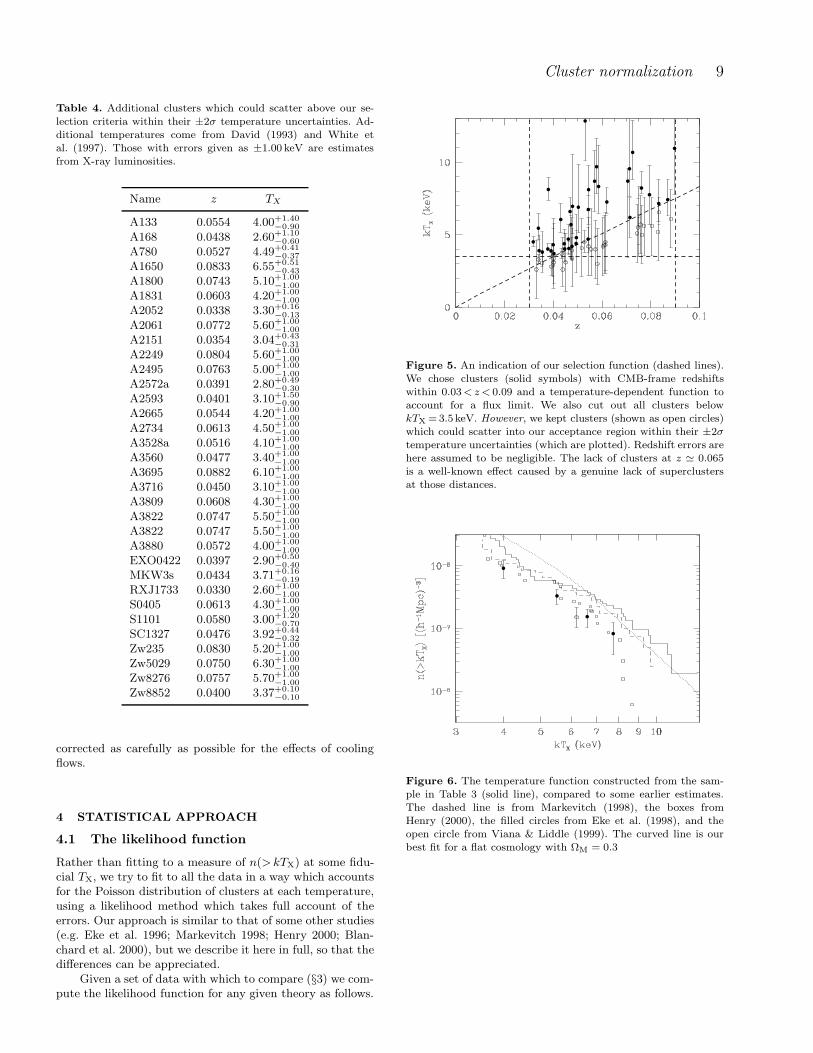
Though we do not use it directly in the analysis (see§4.1) we have constructed the temperature function of oursample for comparison with earlier work. We show this inFig. 6, where we have only used the clusters in Table 3.Some of the other estimates plotted were derived for specificcosmological models or at other redshifts, so they cannot becompared in great detail. However, it is clear that we are ingeneral agreement with the temperature function estimatedby Markevitch (1998), although a little higher. More strikingis that both of these estimates are considerably higher thanthose of Henry (2000) and of Eke et al. (1996) and Viana& Liddle (1999) which are based on the earlier Henry &Arnaud (1991) sample. The main reason for this differenceis the correction for cooling flows. We believe that the mostphysically realistic comparison of the z≃ 0 clusters with theresults of simulations is to correct for cooling flows, since the

full cooling-flow physics is not contained in the simulations.‡

This gives rise to an added complication when carrying outevolutionary studies of the high-z vs low-z samples, sincedetailed information about cooling flows in high-z clusterstends not to exist. However, for our purposes it seems clearthat we should use cluster temperatures which have been

‡ The cooling flow correction applied by White (2000) may over-estimate the temperature for some clusters like A754. However,we decided to stick to the White (2000) results in all cases, forreasons of consistency.

Table 3. Our nearby cluster sample. The data are adapted from

the sample of Markevitch (1998) with White (2000) temperatures,and Struble & Rood (1999) redshifts, as discussed in the text.Reported errors are 1σ. Note that the White (2000) method mayoverestimate the temperature for some clusters for which the ex-istence of a central cooling flow is debatable, e.g. A399, A401,A754, A1775, A3158 and A3562 (M. Markevitch, private com-munication). Removing these clusters has negligible effect on ourresults, and we prefer to use the White (2000) temperatures, whenavailable, for the sake of consistency.

Name z TX

A85 0.0543 6.74+0.50−0.50

A119 0.0430 6.05+0.55−0.43

A193 0.0476 4.20+1.00−0.50

A376 0.0472 5.70+0.31−1.17

A399 0.0712 9.55+1.92−0.96

A401 0.0725 10.68+1.11−0.94

A478 0.0869 7.42+0.71−0.54

A496 0.0317 4.51+0.17−0.15

A576 0.0377 4.02+0.20−0.07

A754 0.0530 12.85+1.77−1.35

A1644 0.0461 4.70+0.49−0.49

A1651 0.0832 7.15+0.84−0.62

A1736 0.0446 4.02+0.67−0.43

A1775 0.0705 8.70+0.42−2.63

A1795 0.0619 7.26+0.51−0.40

A2029 0.0761 8.22+0.58−0.20

A2063 0.0341 3.90+0.51−0.38

A2065 0.0714 6.19+0.70−0.70

A2107 0.0399 4.31+0.57−0.35

A2142 0.0897 10.96+2.56−1.58

A2147 0.0338 5.45+0.51−0.38

A2151a 0.0354 3.80+0.70−0.50

A2255 0.0794 7.76+1.01−1.01

A2256 0.0569 8.69+1.06−1.06

A2589 0.0402 3.70+1.04−1.04

A2657 0.0390 3.89+0.24−0.15

A3158 0.0585 8.33+1.43−0.95

A3266 0.0577 9.69+0.97−0.92

A3376 0.0444 4.38+0.36−0.12

A3391 0.0502 6.90+1.47−0.86

A3395 0.0494 4.80+0.24−0.24

A3532 0.0542 4.70+0.39−0.47

A3558 0.0468 6.60+0.50−0.50

A3562 0.0478 6.96+1.77−0.95

A3571 0.0379 8.12+0.42−0.39

A3667 0.0544 8.11+0.82−0.73

A4059 0.0463 4.05+0.23−0.19

IIZw108 0.0493 4.40+1.00−1.00

Cluster normalization 9

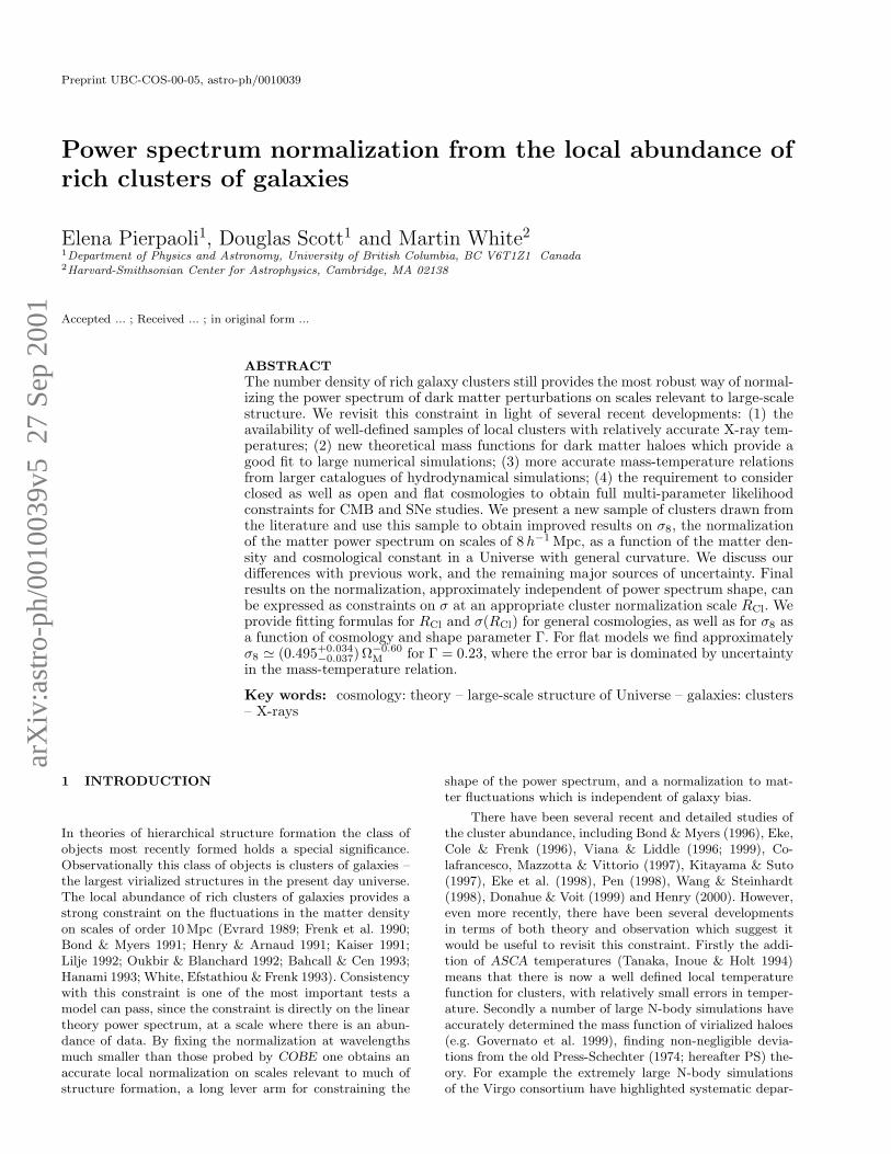
Table 4. Additional clusters which could scatter above our se-

lection criteria within their ±2σ temperature uncertainties. Ad-ditional temperatures come from David (1993) and White etal. (1997). Those with errors given as ±1.00 keV are estimatesfrom X-ray luminosities.

Name z TX

A133 0.0554 4.00+1.40−0.90

A168 0.0438 2.60+1.10−0.60

A780 0.0527 4.49+0.41−0.37

A1650 0.0833 6.55+0.51−0.43

A1800 0.0743 5.10+1.00−1.00

A1831 0.0603 4.20+1.00−1.00

A2052 0.0338 3.30+0.16−0.13

A2061 0.0772 5.60+1.00−1.00

A2151 0.0354 3.04+0.43−0.31

A2249 0.0804 5.60+1.00−1.00

A2495 0.0763 5.00+1.00−1.00

A2572a 0.0391 2.80+0.49−0.30

A2593 0.0401 3.10+1.50−0.90

A2665 0.0544 4.20+1.00−1.00

A2734 0.0613 4.50+1.00−1.00

A3528a 0.0516 4.10+1.00−1.00

A3560 0.0477 3.40+1.00−1.00

A3695 0.0882 6.10+1.00−1.00

A3716 0.0450 3.10+1.00−1.00

A3809 0.0608 4.30+1.00−1.00

A3822 0.0747 5.50+1.00−1.00

A3822 0.0747 5.50+1.00−1.00

A3880 0.0572 4.00+1.00−1.00

EXO0422 0.0397 2.90+0.50−0.40

MKW3s 0.0434 3.71+0.16−0.19

RXJ1733 0.0330 2.60+1.00−1.00

S0405 0.0613 4.30+1.00−1.00

S1101 0.0580 3.00+1.20−0.70

SC1327 0.0476 3.92+0.44−0.32

Zw235 0.0830 5.20+1.00−1.00

Zw5029 0.0750 6.30+1.00−1.00

Zw8276 0.0757 5.70+1.00−1.00

Zw8852 0.0400 3.37+0.10−0.10

corrected as carefully as possible for the effects of coolingflows.

4 STATISTICAL APPROACH

4.1 The likelihood function

Rather than fitting to a measure of n(>kTX) at some fidu-cial TX, we try to fit to all the data in a way which accountsfor the Poisson distribution of clusters at each temperature,using a likelihood method which takes full account of theerrors. Our approach is similar to that of some other studies(e.g. Eke et al. 1996; Markevitch 1998; Henry 2000; Blan-chard et al. 2000), but we describe it here in full, so that thedifferences can be appreciated.

Given a set of data with which to compare (§3) we com-pute the likelihood function for any given theory as follows.

Figure 5. An indication of our selection function (dashed lines).We chose clusters (solid symbols) with CMB-frame redshiftswithin 0.03<z< 0.09 and a temperature-dependent function toaccount for a flux limit. We also cut out all clusters belowkTX =3.5keV. However, we kept clusters (shown as open circles)which could scatter into our acceptance region within their ±2σtemperature uncertainties (which are plotted). Redshift errors arehere assumed to be negligible. The lack of clusters at z ≃ 0.065is a well-known effect caused by a genuine lack of superclustersat those distances.

Figure 6. The temperature function constructed from the sam-ple in Table 3 (solid line), compared to some earlier estimates.The dashed line is from Markevitch (1998), the boxes fromHenry (2000), the filled circles from Eke et al. (1998), and theopen circle from Viana & Liddle (1999). The curved line is ourbest fit for a flat cosmology with ΩM = 0.3

10 E. Pierpaoli, D. Scott & M. White

We break the range of temperatures under considerationinto a large number of bins, chosen to be narrow enoughso that the probability of two clusters occupying the samebin is very small. Then for a given Monte-Carlo realization(§4.2) of the temperatures of the set of clusters we place theclusters into the appropriate temperature bins, giving an oc-cupation number ηi = 0 or 1 for each bin. For a predictednumber density Ni = n(T )dT , depending on our cosmolog-ical parameters, the mean occupation number of each binis µi = NiVi ≪ 1. Here Vi is the volume of space to whichclusters in bin i can be seen:

Vi =Ωs

3

(d32 − d31

), (16)

if the survey solid angle is Ωs, which is 4π(1 − cos 70) ≃8.27 sr here. With a Euclidean assumption d1 = cz1/H0,while

d2 = min

(cz2H0

,

√L(TX)

4πflim

), (17)

where flim is the limiting flux of the survey (2×1014Wm−2)and L(TX) is obtained from the luminosity-temperature re-lation, Eq. (14), given the cluster’s temperature. Then thelikelihood of observing this combination of clusters is simply

lnL =∑

i

[(ηi − 1)µi + ηi ln (1− exp(−µi))] , (18)

where by assumption only one of the two terms is non-zerofor each bin i. This correctly accounts for the Poisson errorsand uses the full temperature information from the sample.

4.2 Monte Carlos

Given that there are non-negligible uncertainties occurringin several places, that the calculation is quite non-linear,and that n(T ) is a steeply falling function, it is important totreat errors carefully. The only reasonable way to do this isthrough a Monte Carlo approach (also emphasized by Viana& Liddle 1999 and Blanchard et al. 2000), which we now de-scribe. Firstly, we choose a temperature for each cluster (inTables 3 and 4) by generating Gaussian random numbers,using the upper and lower error bars each 50 per cent ofthe time. Then we form a new sample by culling all clusterswith temperatures which fail our selection cuts (as describedin §3). Next we adopt a specific M−T relation drawn fromthe central value and systematic range discussed in §2.5,together with an additional scatter, different for each tem-perature considered, arising from the intrinsic scatter in theM−T relation. For each temperature, we use the M−T re-lation to calculate n(T ) according to the mass function inEq. (8).

For each cosmological model considered, we then maxi-mize the likelihood to find a best-fitting normalization fromwhich to determine σ8. This whole process is repeated 1000times to obtain a distribution of σ8 values for each cosmol-ogy.

5 RESULTS

Our main result is the power spectrum normalization as afunction of cosmological model. We quote the normalization

Table 5. Coefficients of the fitting formula, Eq. (20), for the mean

and errors of σ(RCl) = p0Ω−(p1+p2ΩM+p3ΩΛ)M .

parameterp0 p1 p2 p3

mean 0.505 0.150 −0.233 0.048−1σ 0.473 0.124 −0.234 0.053+1σ 0.532 0.171 −0.222 0.044

for the variance on a scale RCl that corresponds to a clus-ter of 6.5 keV forming now. This is advantageous becausethe value of σ(RCl) is almost independent of the power-spectrum shape Γ (see also Blanchard et al. 2000), while atfixed σ(RCl) the value of σ8 can vary by as much as 15 percent as Γ spans the 68 per cent confidence range, 0.19–0.37,of Eisenstein & Zaldarriaga (2001). Fitting formulae accu-rate at the 1 per cent level for RCl and σ(RCl) covering theranges 0.2 ≤ ΩM ≤ 0.8 and 0.3 ≤ ΩΛ ≤ 1 are given by:

RCl = p0 Ω−(p1+p2 ΩM+p3 ΩΛ)M h−1Mpc ; (19)

σCl ≡ σ(RCl) = p0 Ω−(p1+p2 ΩM+p3 ΩΛ)M . (20)

Here ~p = (9.086, 0.354, 0.058, 0.049) gives the coefficients inEq. (19), while those for Eq. (20) can be found in Table 5,along with fits to the ±1σ limits on σ(RCl). The validity ofEq. (20) has been tested also in the case of open (i.e. ΩΛ = 0)and Einstein-de Sitter (i.e. ΩM = 1) models, and for thiswider range of parameters the maximum deviation from thefit is still only 2 per cent. For the concordance model (ΩM =0.3) we find RCl ≃ 14.8 h−1Mpc. A slightly less precise, butsimpler fit for flat models is given by

RCl ≃ 9.0Ω−0.41M h−1Mpc. (21)

This fits to better than 1 per cent over 0.2 ≤ ΩM ≤ 1.For explicit constraints on σ8 we verified that the fol-

lowing equation is a good fit (with a maximum error of 2per cent), in the range 0.19 ≤ Γ ≤ 0.37 (Eisenstein & Zal-darriaga 2001), 0.2 ≤ ΩM ≤ 0.8 and 0.3 ≤ ΩΛ ≤ 1:

σ8 = σCl q0 Ωq1Λ Ω

−(q2+q3ΩM)M Γ(q4+q5ΩM). (22)

Here the vector of coefficients is given by ~q =(1.049, 0.029, 0.546, 0.350, 0.278,−0.312). For flat models(i.e. ΩΛ = 1− ΩM) this corresponds approximately to

σ8 ≃ (0.495+0.034−0.037) Ω

−0.60M (23)

for the value Γ = 0.23 explicitly, and for general Γ:

σCl = 0.462+0.027−0.029Ω

−0.194−0.179

−0.218

M , (24)

where the exponents in brackets refer to the best power-laws for the +1σ and −1σ limits. It is interesting to noticethat, despite the many differences in our approach, this re-sult does not differ dramatically from other studies, such asthose reported in Fig. 7. This is true even for those stud-ies with apparently quite discrepant temperature functions,such as Henry (2000). As we discuss below this is partly dueto the chance cancelation of several small changes affectingthe derived σ8.

Cluster normalization 11

Figure 7. The normalization σ8 for flat cosmologies with shapeparameter fixed at Γ = 0.23 as derived here (solid,red ) with 1–σ limits (dashed red lines), compared with the fits from Viana& Liddle (1999) (dot-dashed dark blue line), Wang & Stein-hardt(1998) (blue 3 dots-dashed), Eke et al. (1996) (dottedgreen), and Borgani et al.(1999) (cyan).

We performed several checks on our results. First wemade sure that analysing the sample using a single (me-dian) redshift did not introduce a significant bias. We splitthe sample into low-z and high-z halves and analysed themindependently. The variation in σCl between the low-z, high-z and combined samples was only 2 per cent for a flat modelwith ΩM = 0.3. We also gradually eliminated clusters withredshift below a threshold z∗, and then above that threshold.The results change smoothly with z∗, implying that the fi-nal result is not dominated by any particular cluster. Finallywe eliminated all clusters below 6 keV (which approximatelyhalves the sample in each Monte-Carlo realization). Whilethe errors increase in this process, the central value onlyincreases by 3–5 per cent (depending on ΩM).

In earlier cluster samples the shape of the temperaturefunction was not obviously well fit by the theoretical predic-tions. Much of this discrepancy has now disappeared thanksto better data. The question remains however as to howmuch the shape of the temperature function affects the fit,rather than for example the overall amplitude at some in-termediate temperature. To address this we have calculatedσCl for flat cosmologies by matching the observed n(>kTX)for TX = 6keV. We found values 2.5–4.5 per cent lower thanfitting to the whole temperature function for TX > 3.5 keV.Thus the shape of the temperature function is being usedin the fit, and shifts the best fitting σCl by a small, butnon-negligible amount.

In Fig. 7 we compare our results with those of Viana &Liddle (1999) and others for flat cosmologies as a function

of ΩM.§ While the Viana & Liddle (1999) best fit is withinour error bars, the shape of the two curves is quite different.

§ Many authors have found similar results which slightly differfrom Viana & Liddle. We choose to focus on their study for com-parison, since they were very explicit about the details of their

Figure 8. The normalization σ8 for flat cosmologies with Γ =0.23 as derived here (solid red line) but with β = 1.17, comparedwith the Viana & Liddle (1999) results (dark blue dot-dashedline) and also compared with their approach but without the in-tegration over formation redshift (blue dashed line).

This discrepancy can be traced to a number of factors: anewer data compilation; our likelihood fit to the entire clus-ter data; our use of the Sheth & Tormen (1999) universalmass function rather than the PS theory; not integratingover formation redshifts; different M−T normalization andscatter; and different sources of errors (in particular Viana& Liddle 1999 included errors in Γ).

We found a relatively symmetric error bar on our finalresults for σCl and σ8, while Viana & Liddle (1999) had avery asymmetric error. It appears that this is mainly due totheir assumed skew distribution for Γ. Another importantdifference is that Viana & Liddle (1999) adopted a lowervalue of β with respect to ours. If we chose β = 1.17, wewould find the same normalization at high ΩM (see Fig. 8).Approximately half of the discrepancy at lower ΩM comesfrom the fact that we have not integrated over ‘formation’redshift, while Viana & Liddle (1999) included such an inte-gration (see Fig. 8). We argued in §2 that including such anintegration in addition to the scatter in the M−T relationwas effectively double counting some of the scatter.

Use of the Sheth & Tormen (1999) or Jenkins etal. (2001) mass function, rather than PS, lowers our resultsby 4–8 per cent (depending on ΩM). Note that the overalleffect of the different mass function may depend on redshift,so that if formation redshift is integrated over then the dis-crepancy may even be in the other direction.

A major source of theoretical uncertainty remains thevalue and distribution of β in the M−T relation of Eq. (13).We show in Fig. 9 how σCl changes as β is scanned from 0.9to 1.5 (with no systematic error) in our reference model withΩM = 0.3 and ΩΛ = 0.7. It is clear that a better estimate ofthe M −T relation would greatly reduce the errors on σCl.It is also clear that to obtain an unbiased estimate of σCl

procedure. See Wang & Steinhardt (1998) for a detailed discus-sion of differences between some other studies.

12 E. Pierpaoli, D. Scott & M. White

Figure 9. The largely Γ-independent normalization σ(RCl) fordifferent values of β in the M−T relation. The error bars indicatethe standard deviation of σ(RCl) arising from all uncertaintiesexcept for the systematic error in β, which is set to zero here.Our adopted central value of β is 1.3.

it is essential to use an appropriate central value and erroron β, which is why we have included both a statistical and‘systematic’ error in our fits (see also Table 6).

An estimate of the uncertainty introduced by variousfactors is shown in Table 6. To obtain the estimates of er-ror budget in this table we ran our code with the sources oferrors described in the first column. The first case for exam-ple is the complete calculation, with all sources of error in-cluded. The second case has only the statistical uncertaintyin the M−T relation, while the uncertainty in the value ofthe cluster temperature and the systematic scatter in theM−T relation were not used. The other cases show whathappens with one or other source of uncertainty excluded.The mean quoted is the mean of the distribution obtainedin each case, while the the errors are obtained by integratingthe normalized distribution until 34 per cent of the area isreached on each side of the mean.

We find that our uncertainty in σ8 is dominated by sys-tematics in the M−T relation (see also Voit 2000). The sta-tistical scatter in the M−T relation has an almost negligibleeffect on the central value and the error. The temperatureerrors themselves give a skewed distribution to σ8, but thiseffect is sub-dominant.

6 CONCLUSIONS

The local abundance of rich clusters of galaxies currentlyprovides one of the strongest constraints on the normaliza-tion of the present day dark matter power spectrum on ascale of ∼ 10Mpc. While there have been numerous detailedstudies of this constraint in the past, recent developmentsin both theory and observation have made it worthwhile torevisit this quantity.

We have calculated the constraint on σ8 arising froma new local sample of X-ray clusters with ASCA temper-atures. We have incorporated the universal mass function

Table 6. For a flat cosmology with ΩM = 0.3 we estimate how

each source of uncertainty affects the mean and the error of ourσCl estimates. M−T |sys and M−T |stat represent the systematicand statistical errors in the M−T relation, while T represents theerror in the temperature of the clusters. The +1σ and −1σ limitsare found from integrating the distribution of 1000 Monte Carlosin each case.

Source of error mean σ(RCl) +1σ −1σ

all 0.581 0.049 0.050M−T |sys 0.575 0.047 0.047M−T |stat 0.570 0.002 0.002T 0.586 0.005 0.018

determined from recent large N-body simulations, which issufficiently different from the PS theory that the cosmologi-cal constraints inferred from cluster abundances change. Wetried to carefully define the relation between mass and X-ray temperature for galaxy clusters, based on the results ofmany different hydrodynamical simulations. Another majordifference with previous work was that we performed all thecomparisons at the ‘observed epoch’ rather than carryingout an integration over ‘formation times’. We also consid-ered general combinations of ΩM and ΩΛ, including closedmodels. Our results are best presented in terms of a nor-malization at the characteristic scale for our sample, RCl,where the normalization is largely independent of the powerspectrum shape.

In the near future we anticipate a dramatic increasein our knowledge of the cosmological parameters fromCMB anisotropy missions. In particular it has been fore-cast (Eisenstein, Hu & Tegmark 1999) that MAP will beable to determine σ8 to 14 per cent, at the same time as con-straining a suite of other parameters. The cluster abundanceconstraint is currently uncertain only at the ∼ 10 per centlevel, and so certainly is a pivotal limit on models – it is alsoan entirely independent constraint (at low z, in the mildlynon-linear regime) compared with the CMB determinations(derived from the purely linear regime at z ≃ 1000). Theuncertainty in the derived σ8 could be dramatically reducedwith improvement in the M−T relation, as well as throughnew X-ray data coming from Chandra and XMM-Newton.

Future X-ray surveys, which go much fainter will leadto an increase in the size and quality of the X-ray data. Weshowed in Fig. 4 that there is lots of volume that was notprobed at, say, 5 keV. For example the ROSAT Bright Sur-vey (Schwope et al. 2000) contains an approximately com-plete flux-limited sample of 302 clusters at |b|> 30, most ofthem lying at low redshift, which would be an excellent data-base if they all had good temperature estimates. More im-portant than just increasing the precision of the X-ray tem-perature measurements is an increase in the quality of data,for the purposes of more fully understanding the comparisonwith models. Better spatial and spectral information fromX-ray clusters should allow more reliable estimates for thevalue of TX which is most appropriate for comparing withthe simulations. In a similar vein, improved optical stud-ies of lensing and velocity dispersions could improve massdeterminations for individual clusters.

Cluster normalization 13

The major improvement will come through a more pre-cise mass-temperature relation for X-ray clusters. This willrequire both the improved data which we can foresee fromChandra and XMM-Newton, and improvements in mod-elling the gas physics relevant for understanding the X-rayproperties of clusters. Eventually we imagine that the datawill be fit more directly to much more ambitious simula-tions – this will be extremely difficult in practice, since awide range of scales needs to be modelled simultaneously.In the meantime the piece-meal approach we have takenhere will continue to be useful. With each of the ingredi-ents, particularly the mass-temperature relation, improvingwith time, the cluster abundance will continue to be a strongconstraint on the normalization of dark matter fluctuationson the ∼ 10Mpc scale.

ACKNOWLEDGMENTS

EP and DS were supported by the Canadian Natural Sci-ences and Engineering Research Council, and MW by theUS National Science Foundation and a Sloan Fellowship.EP is a National Fellow of the Canadian Institute for The-oretical Astrophysics. We would like to thank the Institutefor Theoretical Physics, Santa Barbara for their hospitalitywhile some of this work was carried out. We are indebted toAlain Blanchard, Stefano Borgani, Patrick Henry, AndrewLiddle, Maxim Markevitch and David Weinberg for provid-ing useful comments on an early version of the manuscript.This research has made use of the NASA/IPAC Extragalac-tic Database (NED) which is operated by the Jet Propul-sion Laboratory, California Institute of Technology, undercontract with the National Aeronautics and Space Admin-istration.

REFERENCES

Allen S.W., 1998, MNRAS, 296, 392Bahcall N., Cen R., 1993, ApJ, 407, L49Balogh M.L., Babul A., Patton D.R., 1999, MNRAS, 307, 463Bohringer H., Schuecker P., Guzzo L., Collins C.A., Voges W.,

et al., 2001, A&A, in press, astro-ph/0012266

Bardeen J.M., Bond J.R., Kaiser N., Szalay A.S., 1986, ApJ,304, 15

Blanchard A., Sadat R., Bartlett J.G., Le Dour M., 2000, A&A,362, 809

Bond J.R., Myers S.T., 1991, Trends in Astroparticle Physics,eds. D. Cline, R. Peccei, World Scientific, Singapore, p. 262

Bond J.R., Myers S.T., 1996, ApJS, 103, 63

Borgani S., Rosati P., Tozzi P. Norman C., 1999, ApJ, 517, 40Bryan G.L., Norman M.L., 1998, ApJ, 495, 80Carlberg R.G., Yee H.K.C., Ellingson E., Abraham R., Gravel

P., et al., 1996, ApJ, 462, 32Carroll S.M., Press W.H., Turner E.L., ARAA, 30, 499

Cavaliere A., Menci N., Tozzi P., 1999, MNRAS, 308, 599Cohn J., 1999, Astrophys. & Space Science, 259, 213.Colafrancesco S., Mazzotta P., Vittorio N., 1997, ApJ, 488, 566David L.P., Slyz A., Jones C., Forman W., Vrtilek S.D., et

al. 1993, ApJ, 412, 479

Davis M., Efstathiou G., Frenk C.S., White S.D.M., 1985, ApJ,292, 371

de Grandi S., Bohringer H., Guzzo L., Molendi S., ChincariniG., et al. 1999, ApJ, 514, 148

Donahue M., Voit G.M., 1999, ApJ 523, L137

Ebeling H., Voges W., Bohringer H., Edge A.C., Huchra J.P., etal. 1996, MNRAS, 281, 799

Ebeling H., Edge A.C., Bohringer H., Allen S.W., CrawfordC.S., et al. 1998, MNRAS, 301, 881

Edge A., Stewart G.C., Fabian A.C., Arnaud K.A., 1990,MNRAS, 245, 559

Eisenstein D., Hu W., 1999, ApJ, 511, 5

Eisenstein D., Hu W., Tegmark M., 1999, ApJ, 518, 2

Eisenstein D., Zaldarriaga M., 2001, ApJ, 546, 2[astro-ph/9912149]

Eke V., Cole S., Frenk C.S., 1996, MNRAS, 282, 263

Eke V., Cole S., Frenk C.S., Henry P.J., 1998, MNRAS, 298,1145

Eke V., Navarro J.F., Frenk C.S., 1998, ApJ, 503, 569

Evrard A.E., 1989, ApJ, 341, L71

Evrard A.E., Metzler C., Navarro J.F., 1996, ApJ, 469, 494

Finoguenov A., Arnaud M., David L.P., 2001, ApJ, in press[astro-ph/0009007]

Frenk C.S., White S.D.M., Efstathiou G., Davis M., 1990, ApJ,

351, 10

Frenk C.S., White S.D.M., Bode P., Bond J.R., Bryan G.L., etal. 1999, ApJ, 525, 554

Gardner J.P., 2000, preprint [astro-ph/0006342]

Girardi M., Giuricin G., Mardirossian F., Mezzetti M., BoschinW., 1998a, ApJ, 505, 74

Girardi M., Borgani S., Giuricin G., Mardirossian F., MezzettiM., 1998b, ApJ, 506, 45

Girardi M., Borgani S., Giuricin G., Mardirossian F., MezzettiM., 2000, ApJ, 530, 62

Governato F., Babul A., Quinn T., Tozzi P., Baugh C.M., et al.,1999, MNRAS, 307, 949

Hamilton A.J.S., 2001, MNRAS, 322, 419 [astro-ph/0006089]

Hanami H., 1993, ApJ, 415, 42

Heath D.J., 1977, MNRAS, 179, 351

Henry J.P., 2000, ApJ, 534, 565

Henry J.P., Arnaud K.A., 1991, ApJ, 372, 410

Horner D.J., Mushotsky R.F., Scharf C.A., 1999, ApJ, 520, 78

Irwin J.A, Bregman J.N., 2000, ApJ, 538, 543

Irwin J.A, Bregman J.N., Evrard A.A., 1999, ApJ, 519, 518

Jenkins A., Frenk C.S., White S.D.M., Colberg J.M., Cole S.,Evrard A.E., Yoshida N., 2001, MNRAS, 321, 371[astro-ph/0005260]

Kaiser N., 1991, ApJ, 383, 104

Kitayama T., Suto Y., 1997, ApJ, 490, 557

Lahav O., Rees M.J., Lilje P.B., Primack J.R., 1991, MNRAS,251, 128

Liddle A., Lyth D., 2000, Cosmological Inflation and Large-ScaleStructure, Cambridge University Press, Cambridge.

Lilje P.B., 1992, ApJ, 386, L33

Markevitch M., 1998, ApJ, 504, 27

Mathiesen B.F., 2000, MNRAS, submitted [astro-ph/0012117]

Mathiesen B.F. & Evrard A.E., 2001, ApJ, 546, 100[astro-ph/0004309]

Mohr J.J., Evrard A.E., 1997, ApJ, 491, 38

Molnar S.M., Jahoda K., 2000, [astro-ph/0002270]

Navarro J.F., Frenk C.S., White S.D.M., 1996, ApJ, 462, 563

Nevalainen J., Markevitch M., Forman W., 2000, ApJ, 532, 694[astro-ph/9911369]

Ostriker J.P., Steinhardt P.S., 1995, Nature, 377, 600

Oukbir J., Blanchard A., 1992, A&A, 262, L21

Peacock J.A., 1999, Cosmological Physics, CambridgeUniversity Press, Cambridge.

Peebles, P.J.E., 1993, Principles of Physical Cosmology,Princeton University Press, Princeton, chapter 25.

Pen U.-L., 1998, ApJ, 498, 60

Press W.H., Schechter P., 1974, ApJ, 187, 452

Reiprich T.H., Bohringer H., 1999, 19th Texas Symposium on

14 E. Pierpaoli, D. Scott & M. White

Relativistic Astrophysics and Cosmology, ed. J. Paul,T. Montmerle, E. Aubourg, in press

Schwope A.D., Hasinger G., Lehmann I., Schwarz R., BrunnerH. et al. 2000, Astron. Nach., 321, 1

Sheth R.K., Mo H.J., Tormen G., 2001, MNRAS, 323, 1[astro-ph/9907024]

Sheth R.K., Tormen G., 1999, MNRAS, 308, 119Smail I., Ellis R.S., Dressler A., Couch W.J., Oemler A., et al.,

1997, ApJ, 479, 70Struble M.F., Rood H., 1999, ApJS, 125, 35Tanaka Y., Inoue H., Holt S.S., 1994, PASJ, 46, L37

Thomas P.A., Muanwong O., Pearce F.R., Couchman H.M.P.,Edge A.C., et al., submitted to MNRAS [astro-ph/0007348]

Tittley E.R., Couchman H.M.P., 2000, submitted to MNRAS[astro-ph/9911365]

Viana P.T.P., Liddle A., 1996, MNRAS, 281, 323Viana P.T.P., Liddle A., 1999, MNRAS, 303, 535Voit G.M., 2000, ApJ, 543, 113Wang L., Steinhardt P.J., 1998, ApJ, 508, 483White D.A., 2000, MNRAS, 312, 663White D.A., Buote D.A., 2000, MNRAS, 312, 649White D.A., Jones C., Forman W., 1997, MNRAS, 292, 419White M., Scott D., 1996, ApJ, 459, 415White M., Scott D., Pierpaoli E., 2000, ApJ, 545, 1White S.D.M., Efstathiou G., Frenk C.S., 1993, MNRAS, 262,

1023Wu X.-P., Chiueh T., Fang L.-Z., Xue Y.-J., 1998, MNRAS,

301, 861Xue Y.-J., Wu X.-P., 2000, ApJ, 538, 65Yoshikawa K., Jing Y.P., Suto Y., 2000, ApJ, 535, 593