arX

iv:a

stro

-ph/

0703

134v

2 1

4 M

ar 2

007

Binaries in the Kuiper Belt

Keith S. NollSpace Telescope Science Institute

William M. GrundyLowell Observatory

Eugene I. ChiangUniversity of California, Berkeley

Jean-Luc MargotCornell University

Susan D. KernSpace Telescope Science Institute

Accepted for publication inThe Kuiper BeltUniversity of Arizona Press, Space Science Series

Binaries have played a crucial role many times in the historyof modern astronomy andare doing so again in the rapidly evolving exploration of theKuiper Belt. The large fraction oftransneptunian objects that are binary or multiple, 48 suchsystems are now known, has beenan unanticipated windfall. Separations and relative magnitudes measured in discovery imagesgive important information on the statistical properties of the binary population that can berelated to competing models of binary formation. Orbits, derived for 13 systems, provide adetermination of the system mass. Masses can be used to derive densities and albedos whenan independent size measurement is available. Angular momenta and relative sizes of themajority of binaries are consistent with formation by dynamical capture. The small satellitesof the largest transneptunian objects, in contrast, are more likely formed from collisions.Correlations of the fraction of binaries with different dynamical populations or with otherphysical variables have the potential to constrain models of the origin and evolution of thetransneptunian population as a whole. Other means of studying binaries have only begun to beexploited, including lightcurve, color, and spectral data. Because of the several channels forobtaining unique physical information, it is already clearthat binaries will emerge as one of themost useful tools for unraveling the many complexities of transneptunian space.

1. HISTORY AND DISCOVERY

Ever since Herschel noticed, two hundred years ago, thatgravitationally bound stellar binaries exist, the search forbinaries has followed close on the heels of the discoveryof each new class of astronomical object. The reasons forsuch searches are, of course, eminently practical. Binary or-bits provide determinations of system mass, a fundamentalphysical quantity that is otherwise difficult or impossibletoobtain. The utilization of binaries in stellar astronomy hasenabled countless applications including Eddington’s land-mark mass-luminosity relation. Likewise, in planetary sci-ence, bound systems have been extensively exploited; theyhave been used, for example, to determine the masses ofplanets and to make Roemer’s first determination of thespeed of light. The statistics of binaries in astronomical

populations can be related to formation and subsequent evo-lutionary and environmental conditions.

Searches for bound systems among the small body pop-ulations in the solar system has a long and mostly fruitlesshistory that has been summarized in several recent reviews(Merline et al., 2002; Noll, 2004, 2006;Richardson andWalsh, 2005). But the discovery of thesecondtransnep-tunian binary (TNB), 1998 WW31 (Veillet et al., 2001)marked the start of a landslide of discovery that shows nosigns of abating.

1.1 Discovery and Characterization of Charon

The first example of what we would now call a TNBwas discovered during a very different technological epochthan the present, prior to the widespread astronomical use

1

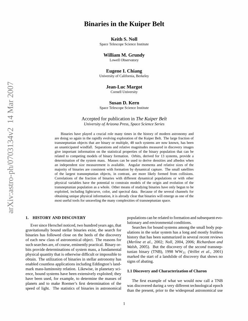
2002 GZ311999 OJ4

(42355) Typhon/Echidna2001 FL185

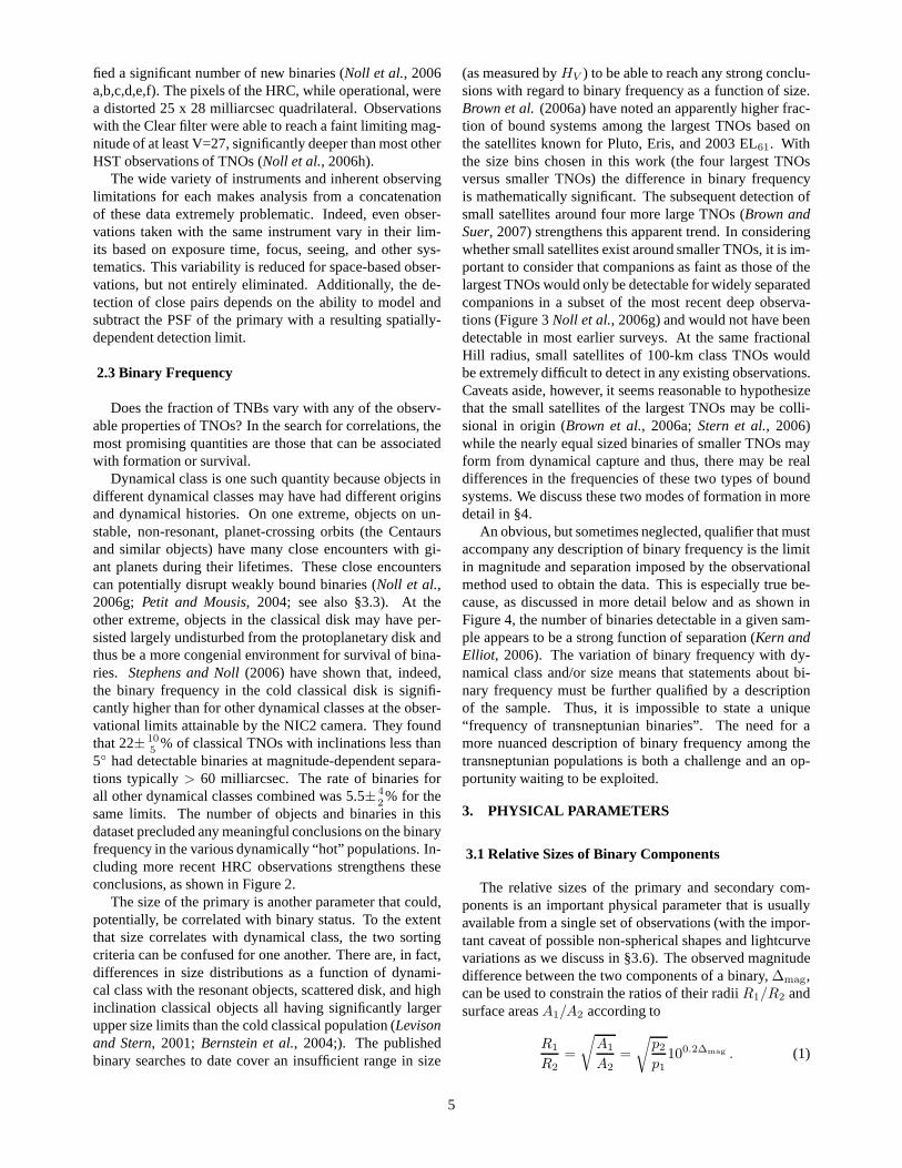
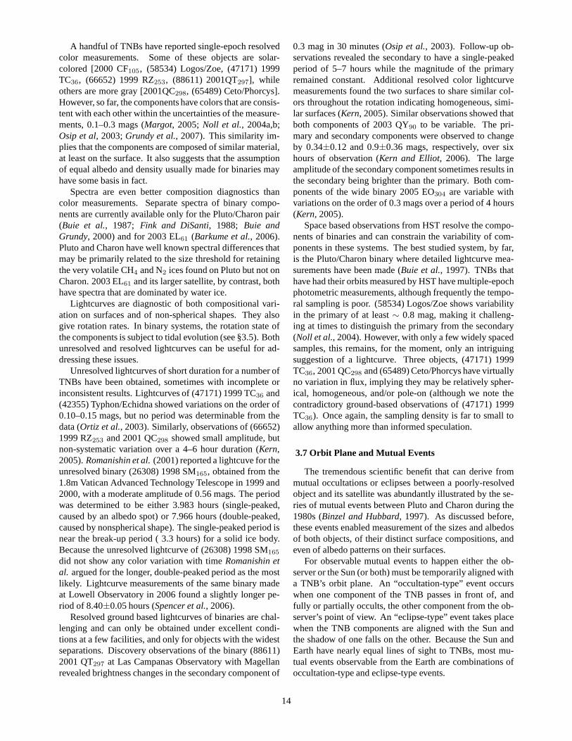
Fig. 1.—Images of 2001 FL185 (top-left), (42355) Typhon/Echidna (top-right), 1999 OJ4 (bottom-left), and 2002 GZ31 (bottom-right).The images shown are each combinations of four separate 300 sexposures taken with the High Resolution Camera on HST. The ditheredexposures have been combined using multidrizzle. The images are shown with a linear grayscale normalized to the peak pixel. Thepixels in the drizzled images are 25 milliarcsec on a side in anon-distorted coordinate frame. Each of the four panels is 1arcsec square.Images are oriented in detector coordinates.

of CCD arrays. The discovery of Charon (Christy and Har-rington, 1978) on photographic plates taken for Pluto as-trometry heralded a spectacular flourishing of Pluto science,and offered a glimpse of the tremendous potential of TNBsto contribute to Kuiper belt science in general.

Charon’s orbit (Christy and Harrington, 1978, 1980) re-vealed the system mass, which up until then had been es-timated via other methods, with wildly divergent results.About the same time, spectroscopy revealed the presenceof methane on Pluto (Cruikshank et al, 1976) indicating ahigh albedo, small size, and the possible existence of an at-mosphere. Observations of occultations of stars by Plutoconfirmed its small size (Millis et al., 1993) and enableddirect detection of the atmosphere (Hubbard et al., 1988).

The orbit plane of Charon, as viewed from the Earth,was oriented edge-on within a few years of Charon’s dis-covery. This geometry happens only twice during Pluto’s248 year orbit, so its occurrence just after Charon’s dis-covery was fortuitous. Mutual events, when Charon (or itsshadow) passed across the face of Pluto, or Pluto (or itsshadow) masked the view of Charon, were observable from1985 through 1990 (Binzel and Hubbard, 1997). From thetiming of these events and from the changes in observableflux during them, much tighter constraints on the sizes andalbedos of Pluto and Charon were derived (e.g. Young andBinzel, 1994). Mutual events also made it possible to dis-tinguish the surface compositions of Pluto and Charon (e.g.Buie et al., 1987;Fink and DiSanti, 1988), by comparingreflectance spectra of the two objects blended together withspectra of Pluto alone, when Charon was completely hidden

from view. From subtle variations in flux as Charon blockeddifferent regions of Pluto’s surface (and vice versa), mapsof albedo patterns on the faces of the two objects were con-structed (e.g. Buie et al., 1997;Young et al., 1999). The mu-tual events are now over and will not be repeated during ourlifetimes, but telescope and detector technology continuetheir advance. For relatively well-separated, bright TNBslike Pluto and Charon, it is now feasible to study them asseparate worlds even without the aid of mutual events (e.g.Brown and Calvin, 2000;Buie and Grundy, 2000). Just asthe discovery of Charon propelled Pluto science forward,the recent study of two additional moons of Pluto (Weaveret al., 2006) can be expected to give another boost to Plutoscience, by enabling detailed studies of the dynamics of thesystem (Buie et al., 2006;Lee and Peale, 2006), and pro-viding new constraints on formation scenarios (e.g. Canup,2005;Ward and Canup, 2006).

1.2 Discovery of Binaries

The serendipitous discovery of the second TNB, 1998WW31 (Veillet et al., 2001) marked a breakthrough for bi-naries in the Kuiper Belt. It immediately provided a contextfor Pluto/Charon as a member of a group of similar systemsrather than as a unique oddity. The relatively large sep-aration and size of the secondary dispelled the notion thatKuiper Belt satellites would all be small, faint, and difficult-to-resolve collision fragments. Some, at least, were de-tectable from the ground with moderately good observingconditions as had been foreseen byToth (1999). The next

2

two discovered TNBs were just such systems (Elliot et al.,2001;Kavelaars et al., 2001).

The first conscious search for satellites of transneptunianobjects (TNOs) was carried out by M. Brown and C. Trujillousing the Space Telescope Imaging Spectrograph (STIS) onthe Hubble Space Telescope (HST) starting in August 2000(Trujillo and Brown, 2002;Brown and Trujillo, 2002). Aseries of large surveys with HST followed producing thediscovery of most of the known TNBs (e.g.Noll et al.,2002a,b,c, 2003;Stephens et al., 2004;Stephens and Noll,2006;Noll et al., 2006a,b,c,d, e,f; Figure 1).

Large ground-based surveys – Keck (Schaller andBrown, 2003), Deep Ecliptic Survey (DES) followup atMagellan (Millis et al., 2002; Ellliot et al., 2005 ), andthe Canada-France Ecliptic Plane Survey (CFEPS;Allenet al., 2006) – have produced a few detections. Thoughsignificantly less productive because of the limited angularresolution possible from the ground compared to HST, thesheer number of objects observed by these surveys makesthem a valuable statistical resource (Kern and Elliot, 2006).Both space- and ground-based discoveries are described indetail in §2.2.

Binaries may also be “discovered” theoretically.Agnorand Hamilton(2006) have shown that the most likely expla-nation for the origin of Neptune’s retrograde satellite Tritonis the capture of one component of a binary that encoun-tered the giant planet. The viability of this model is en-abled by the paradigm-shifting realization that binaries inthe transneptunian region are common.

2. INVENTORY

Much can be learned about binaries and the environmentin which they formed from simple accounting. The fractionof binaries in the transneptunian population is far higherthan anyone guessed a decade ago when none were yet rec-ognized (except for Pluto/Charon), and considerably higherthan was thought even four years ago as the first spate ofdiscoveries was being made. As the number of binarieshas climbed, it has become apparent that stating the frac-tion of binaries is not a simple task. The fraction in a givensample is strongly dependent on a number of observationalfactors, chiefly angular resolution and sensitivity. To addtothe complexity, TNOs can be divided into dynamical groupswith possibly differing binary fractions. Thus, the fractionof binaries in a particular sample also depends on the mixof dynamical classes in the sample. Perversely, perhaps, thebrightest TNOs, and thus the first to be sampled, belong todynamical classes with a lower overall fraction of sizablebinary companions. Other dependencies may also help de-termine the fraction and nature of binaries and multiples;for example, very small, possibly collision-produced com-panions appear to be most likely around the largest of theTNOs. The current inventory of TNBs, while impressivecompared to just a few years ago, remains inadequate toaddress all of the questions one would like to ask.

2.1 Current Inventory of Transneptunian Binaries

As of February 2007, more than 40 TNO and Centaur bi-naries had been announced through the International Astro-nomical Union Circulars (IAUC) and/or other publications.Additional binaries are not yet documented in a publication.All of the binaries of which we are aware are compiled inTable 1. References listed are generally the discovery an-nouncement, when available. Values for separation and rel-ative magnitude were recalculated for many of the objectsand supersede earlier published values. The osculating he-liocentric orbital parametersa⊙, e⊙, andi⊙ are listed aswell as the dynamical class. For the latter we have followedthe DES convention (Elliot et al., 2005), with the resonantobjects identified by their specific resonance asn:m, wheren refers to the mean motion of Neptune. Classical objectson orbits of low inclination and eccentricity are designatedC. Classical objects with an integrated average inclinationi > 5 relative to the invariable plane are denoted byH .Objects in the scattered disk are labelledS or X depend-ing on whether their Tisserand parameter,T , is less than orgreater than 3. The Tisserand parameter relative to Neptuneis defined asTN = aN/a + 2[(1 − e2)a/aN ]1/2 cos(i)wherea,e, andi are the heliocentric semimajor axis, eccen-tricity, and inclination of the TNO andaN is the semimajoraxis of Neptune. Objects in the extended scattered disk,X ,have the additional requirement of a time-averaged eccen-tricity greater than 0.2. Centaurs and Centaur-like1 objects,labelled ¢, are on unstable, non-resonant, planet-crossingorbits and are, therefore, dynamically young. In Table 1 welist the objects in three broad dynamical groupings, Classi-cal, Scattered, and Resonant. The Classical grouping in-cludes all Classical objects regardless of inclination,i.e.both Hot and Cold Classicals. The Resonant group includesall objects verified to be in mean motion resonances by nu-merical integration. The Scattered group includes both Nearand Extended Scattered objects and the Centaurs. Withineach group we have ordered the objects by absolute magni-tude,HV .

In addition to the dynamical class and osculating he-liocentric orbital elements of the binaries, we list in Ta-ble 1 three additional measurements available for all of theknown binaries: 1.) The reported separation at discovery(in arcsec) is shown with the error in the final significantdigit in parentheses. Separations reported without an errorestimate are shown in italics. As we discuss in more detailbelow in §3.3, the separation at discovery is not an intrinsicproperty of binary orbits, but can be useful for estimatingthe distribution of binary semimajor axes. 2.) The magni-tude difference,∆mag, can be used to derive the size ratioof the components (with the customary assumption of equalalbedos). Once again, errors in the final digit are shown in

1Centaur-like objects are in unstable, non-resonant, giant-planet-crossingorbits just like the Centaurs, but have a semimajor axis greater than 30.1AU. There is currently disagreement on what this class of objects shouldbe called. Because of their similarly unstable orbits, we follow the DESconvention and group them with Centaurs.

3

parentheses, and estimated quantities are in italics. 3.) Theabsolute magnitude,HV , is taken from the Minor PlanetCenter (MPC) and applies to the combined light of the un-resolved binary. Better measurements ofHV are availablefor some objects (Romanishin and Tegler, 2005), but for thesake of uniformity we use the MPC values for all objects.HV can provide a determination of the size if the albedo isknown or can be estimated. However, the range of albedo inthe transneptunian population is large (Grundy et al., 2005)as is the phase behavior (Rabinowitz et al., 2007) makingany such estimate risky (see also the chapters byStansberryet al. andBelskaya et al.).

2.2 Large Surveys, Observational Limits, and Bias

Several large surveys have produced the discovery oflarge fractions of the known TNBs. Observational limitsare, to first order, a function of the telescope and instrumentused for the observations. This is more easily characterizedfor space-based instruments than for ground-based surveys,but approximate limits for the latter can be estimated.

The largest semi-uniform ground-based survey of TNOsthat has been systematically searched for binaries is theDeep Ecliptic Survey (Millis et al., 2002; Elliot et al.,2005).Kern and Elliot(2006) searched 634 unique objectsfrom the DES survey and identified 1. These observationswere made with 4m telescopes at CTIO and KPNO utiliz-ing wide field Mosaic cameras (Muller et al., 1998) with0.5 arcsec pixels. Median seeing for the entire data set was1.65 arcsec (Kern, 2005) and effectively sets the detectionlimit on angular separation. Magnitude limits in the broadV R filter for a well-separated secondary vary, dependingon seeing, fromV R = 23 toV R = 24.

Follow-up observations of 212 DES objects made withthe Magellan telescopes to improve astrometry were alsosearched for undetected binaries (Kern and Elliot, 2006).Most observations were made with the MagIC camera (Osipet al., 2004) which has a pixel scale of 0.069 arcsec.Kern(2005) reports the median seeing for these observations was0.7 arcsec with a magnitude limit similar to the DES survey.Of the 212 objects observed with Magellan, 3 were found tobe binaries (Osip et al., 2003,Kern and Elliot, 2005, 2006).

The Keck telescope survey reported bySchaller andBrown(2003) observed 150 objects and found no new bina-ries. The observational limits for this survey have not beenpublished; they are probably similar to the DES as the pri-mary limiting factor is seeing.

The target lists for the three large ground-based surveyshave not been published and it is unclear how much over-lap there may be. However, even duplicate observationsof an individual target can be useful since some TNBs areknown to have significantly eccentric or edge-on orbits andare, therefore, variable in their detectability. The one firmconclusion, however, that can be reached from these datais that binaries separated sufficiently for detection with un-corrected ground-based observations are uncommon, occur-ring around 1–2% of TNOs at most.

The most productive tool for finding TNBs is the HSTwhich has found 41 of the 52 companions listed in Table 1.The combination of high angular resolution, high sensitiv-ity, and stable point-spread-function (PSF) make it ideallymatched to the requirements for finding and studying TNBs.The first conscious search for TNBs using HST was carriedout in August 2000–January 2001 in a program that lookedat just 2 TNOs and found no companions. Two other smallprograms executed between October 1997–September 1998observed 8 TNOs with the potential to identify a binary, hadthere been one among the objects observed.

The first moderate-scale program to search for binariesused STIS in imaging mode to search for binaries around25 TNOs from August 2001–August 2002. This programfound 2 binaries, both relatively faint companions to the res-onant TNOs (47171) 1999 TC36 and (26308) 1998 SM165(Trujillo and Brown, 2002;Brown and Trujillo, 2002). TheSTIS imaging mode has a pixel scale of 50 milliarcsec mak-ing it possible to directly resolve objects separated by ap-proximately 100 milliarcsec or more. In principle, PSFanalysis can detect binaries at significantly smaller sepa-rations in HST data because of the stability of the PSF(Stephens and Noll, 2006). The STIS data were obtainedwithout moving the telescope to track the target’s motion.The TNOs observed this way drift measurably during expo-sures, complicating the PSF analysis for these data.

From July 2001–June 2002 75 separate TNOs were ob-served with WFPC2 in a program designed to obtain V, R,and I band colors (Stephens et al., 2003); 3 of these werefound to be binary. To achieve better sensitivity and becauseof the relatively large uncertainties in TNO orbits at thetime, the targets were observed with the WF camera with100 milliarcsec pixels. The sensitivity to faint companionsfor these data has not been fully quantified and exposuretimes were varied depending on the anticipated brightnessof the TNO so that, in any case, the limits vary. Typical pho-tometric uncertainties ranged from 3–8% for V magnitudesthat ranged from 21.9 to 25.1 with a median magnitude of23.6.

NICMOS was used to observe 82 separate TNOs fromAugust 2002 through June 2003. Observations were madewith the NIC2 camera at a 75 milliarcsec pixel scale. Twobroad filters, the F110W and F160W, approximating the Jand H band filters, were used in the observations. A to-tal of 9 new binary systems were identified from this dataset, 3 of which were resolved and visible in the unpro-cessed data. The other 6 binaries were identified from aprocess of PSF fitting that enabled a significant increasein detectivity beyond the usual Nyquist limit with a sep-aration/relative brightness/total brightness function that iscomplex and modeled with simulated binaries. Several ofthe binaries identified in this way have been subsequentlyresolved with the higher resolution HRC, verifying the ac-curacy of the analysis of the NICMOS data (Stephens andNoll, 2006).

From July 2005 through January 2007, HST’s HRC wasused to look at more than 100 TNOs. This program identi-

4

fied a significant number of new binaries (Noll et al., 2006a,b,c,d,e,f). The pixels of the HRC, while operational, werea distorted 25 x 28 milliarcsec quadrilateral. Observationswith the Clear filter were able to reach a faint limiting mag-nitude of at least V=27, significantly deeper than most otherHST observations of TNOs (Noll et al., 2006h).

The wide variety of instruments and inherent observinglimitations for each makes analysis from a concatenationof these data extremely problematic. Indeed, even obser-vations taken with the same instrument vary in their lim-its based on exposure time, focus, seeing, and other sys-tematics. This variability is reduced for space-based obser-vations, but not entirely eliminated. Additionally, the de-tection of close pairs depends on the ability to model andsubtract the PSF of the primary with a resulting spatially-dependent detection limit.

2.3 Binary Frequency

Does the fraction of TNBs vary with any of the observ-able properties of TNOs? In the search for correlations, themost promising quantities are those that can be associatedwith formation or survival.

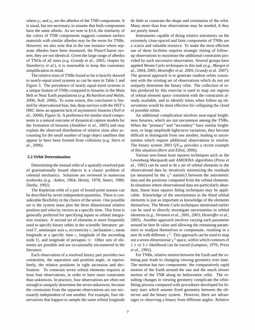
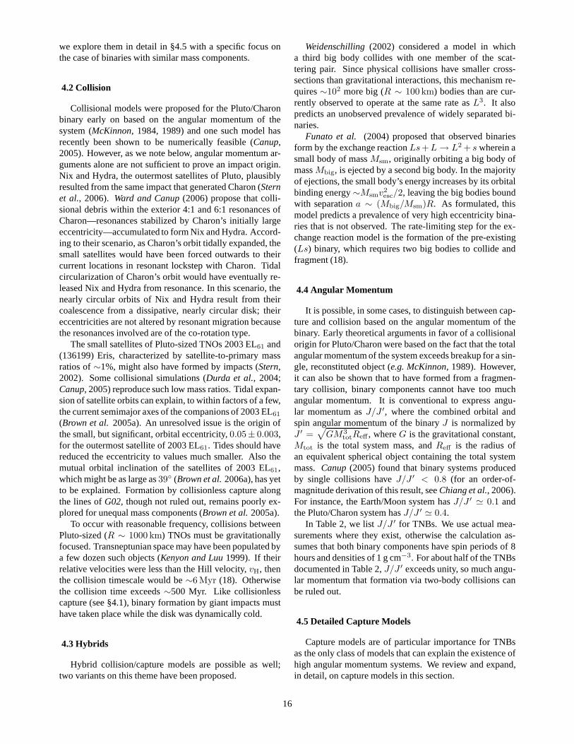
Dynamical class is one such quantity because objects indifferent dynamical classes may have had different originsand dynamical histories. On one extreme, objects on un-stable, non-resonant, planet-crossing orbits (the Centaursand similar objects) have many close encounters with gi-ant planets during their lifetimes. These close encounterscan potentially disrupt weakly bound binaries (Noll et al.,2006g; Petit and Mousis, 2004; see also §3.3). At theother extreme, objects in the classical disk may have per-sisted largely undisturbed from the protoplanetary disk andthus be a more congenial environment for survival of bina-ries. Stephens and Noll(2006) have shown that, indeed,the binary frequency in the cold classical disk is signifi-cantly higher than for other dynamical classes at the obser-vational limits attainable by the NIC2 camera. They foundthat 22± 10

5% of classical TNOs with inclinations less than

5 had detectable binaries at magnitude-dependent separa-tions typically> 60 milliarcsec. The rate of binaries forall other dynamical classes combined was 5.5± 4

2% for the

same limits. The number of objects and binaries in thisdataset precluded any meaningful conclusions on the binaryfrequency in the various dynamically “hot” populations. In-cluding more recent HRC observations strengthens theseconclusions, as shown in Figure 2.

The size of the primary is another parameter that could,potentially, be correlated with binary status. To the extentthat size correlates with dynamical class, the two sortingcriteria can be confused for one another. There are, in fact,differences in size distributions as a function of dynami-cal class with the resonant objects, scattered disk, and highinclination classical objects all having significantly largerupper size limits than the cold classical population (Levisonand Stern, 2001; Bernstein et al., 2004;). The publishedbinary searches to date cover an insufficient range in size

(as measured byHV ) to be able to reach any strong conclu-sions with regard to binary frequency as a function of size.Brown et al.(2006a) have noted an apparently higher frac-tion of bound systems among the largest TNOs based onthe satellites known for Pluto, Eris, and 2003 EL61. Withthe size bins chosen in this work (the four largest TNOsversus smaller TNOs) the difference in binary frequencyis mathematically significant. The subsequent detection ofsmall satellites around four more large TNOs (Brown andSuer, 2007) strengthens this apparent trend. In consideringwhether small satellites exist around smaller TNOs, it is im-portant to consider that companions as faint as those of thelargest TNOs would only be detectable for widely separatedcompanions in a subset of the most recent deep observa-tions (Figure 3Noll et al., 2006g) and would not have beendetectable in most earlier surveys. At the same fractionalHill radius, small satellites of 100-km class TNOs wouldbe extremely difficult to detect in any existing observations.Caveats aside, however, it seems reasonable to hypothesizethat the small satellites of the largest TNOs may be colli-sional in origin (Brown et al., 2006a;Stern et al., 2006)while the nearly equal sized binaries of smaller TNOs mayform from dynamical capture and thus, there may be realdifferences in the frequencies of these two types of boundsystems. We discuss these two modes of formation in moredetail in §4.

An obvious, but sometimes neglected, qualifier that mustaccompany any description of binary frequency is the limitin magnitude and separation imposed by the observationalmethod used to obtain the data. This is especially true be-cause, as discussed in more detail below and as shown inFigure 4, the number of binaries detectable in a given sam-ple appears to be a strong function of separation (Kern andElliot, 2006). The variation of binary frequency with dy-namical class and/or size means that statements about bi-nary frequency must be further qualified by a descriptionof the sample. Thus, it is impossible to state a unique“frequency of transneptunian binaries”. The need for amore nuanced description of binary frequency among thetransneptunian populations is both a challenge and an op-portunity waiting to be exploited.

3. PHYSICAL PARAMETERS

3.1 Relative Sizes of Binary Components

The relative sizes of the primary and secondary com-ponents is an important physical parameter that is usuallyavailable from a single set of observations (with the impor-tant caveat of possible non-spherical shapes and lightcurvevariations as we discuss in §3.6). The observed magnitudedifference between the two components of a binary,∆mag,can be used to constrain the ratios of their radiiR1/R2 andsurface areasA1/A2 according to

R1

R2

=

√

A1

A2

=

√

p2

p1

100.2∆mag . (1)

5

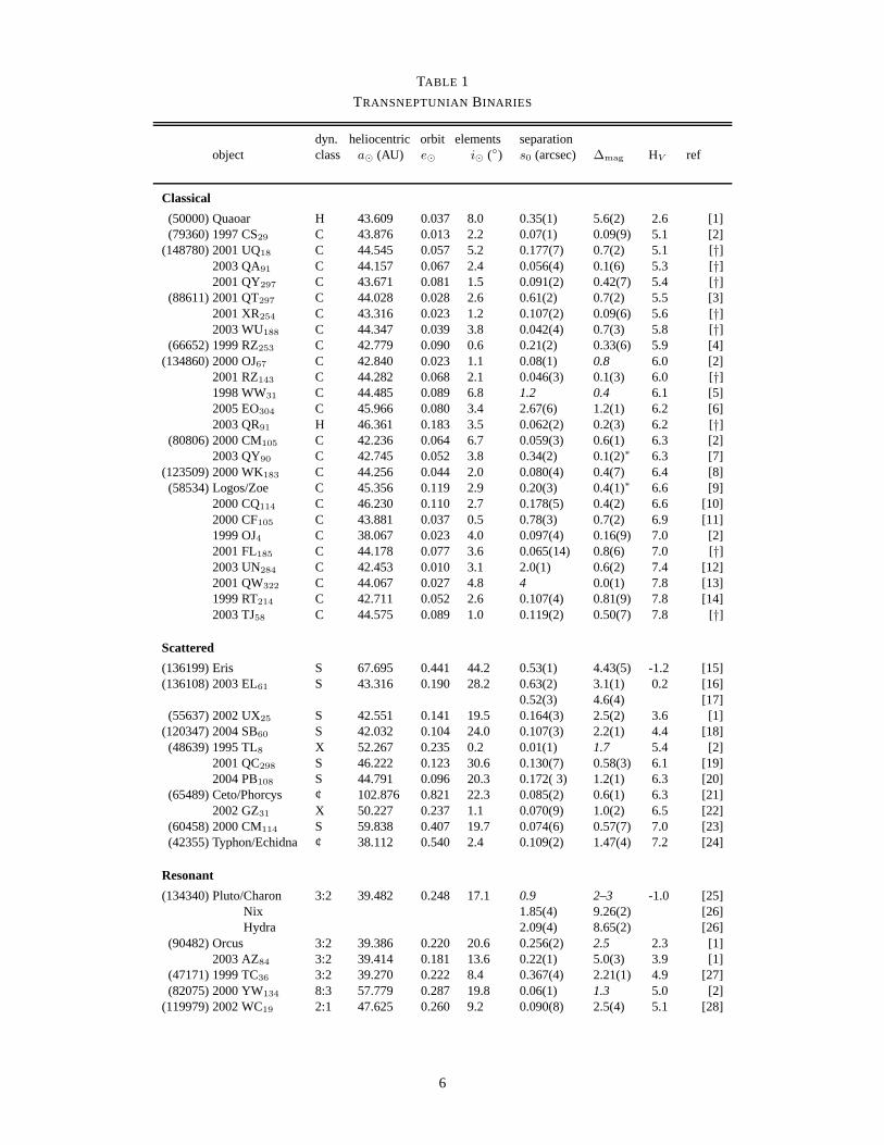
TABLE 1

TRANSNEPTUNIAN BINARIES

dyn. heliocentric orbit elements separationobject class a⊙ (AU) e⊙ i⊙ () s0 (arcsec) ∆mag HV ref

Classical

(50000) Quaoar H 43.609 0.037 8.0 0.35(1) 5.6(2) 2.6 [1](79360) 1997 CS29 C 43.876 0.013 2.2 0.07(1) 0.09(9) 5.1 [2]

(148780) 2001 UQ18 C 44.545 0.057 5.2 0.177(7) 0.7(2) 5.1 [†]2003 QA91 C 44.157 0.067 2.4 0.056(4) 0.1(6) 5.3 [†]2001 QY297 C 43.671 0.081 1.5 0.091(2) 0.42(7) 5.4 [†]

(88611) 2001 QT297 C 44.028 0.028 2.6 0.61(2) 0.7(2) 5.5 [3]2001 XR254 C 43.316 0.023 1.2 0.107(2) 0.09(6) 5.6 [†]2003 WU188 C 44.347 0.039 3.8 0.042(4) 0.7(3) 5.8 [†]

(66652) 1999 RZ253 C 42.779 0.090 0.6 0.21(2) 0.33(6) 5.9 [4](134860) 2000 OJ67 C 42.840 0.023 1.1 0.08(1) 0.8 6.0 [2]

2001 RZ143 C 44.282 0.068 2.1 0.046(3) 0.1(3) 6.0 [†]1998 WW31 C 44.485 0.089 6.8 1.2 0.4 6.1 [5]2005 EO304 C 45.966 0.080 3.4 2.67(6) 1.2(1) 6.2 [6]2003 QR91 H 46.361 0.183 3.5 0.062(2) 0.2(3) 6.2 [†]

(80806) 2000 CM105 C 42.236 0.064 6.7 0.059(3) 0.6(1) 6.3 [2]2003 QY90 C 42.745 0.052 3.8 0.34(2) 0.1(2)∗ 6.3 [7]

(123509) 2000 WK183 C 44.256 0.044 2.0 0.080(4) 0.4(7) 6.4 [8](58534) Logos/Zoe C 45.356 0.119 2.9 0.20(3) 0.4(1)∗ 6.6 [9]

2000 CQ114 C 46.230 0.110 2.7 0.178(5) 0.4(2) 6.6 [10]2000 CF105 C 43.881 0.037 0.5 0.78(3) 0.7(2) 6.9 [11]1999 OJ4 C 38.067 0.023 4.0 0.097(4) 0.16(9) 7.0 [2]2001 FL185 C 44.178 0.077 3.6 0.065(14) 0.8(6) 7.0 [†]2003 UN284 C 42.453 0.010 3.1 2.0(1) 0.6(2) 7.4 [12]2001 QW322 C 44.067 0.027 4.8 4 0.0(1) 7.8 [13]1999 RT214 C 42.711 0.052 2.6 0.107(4) 0.81(9) 7.8 [14]2003 TJ58 C 44.575 0.089 1.0 0.119(2) 0.50(7) 7.8 [†]

Scattered

(136199) Eris S 67.695 0.441 44.2 0.53(1) 4.43(5) -1.2 [15](136108) 2003 EL61 S 43.316 0.190 28.2 0.63(2) 3.1(1) 0.2 [16]

0.52(3) 4.6(4) [17](55637) 2002 UX25 S 42.551 0.141 19.5 0.164(3) 2.5(2) 3.6 [1]

(120347) 2004 SB60 S 42.032 0.104 24.0 0.107(3) 2.2(1) 4.4 [18](48639) 1995 TL8 X 52.267 0.235 0.2 0.01(1) 1.7 5.4 [2]

2001 QC298 S 46.222 0.123 30.6 0.130(7) 0.58(3) 6.1 [19]2004 PB108 S 44.791 0.096 20.3 0.172( 3) 1.2(1) 6.3 [20]

(65489) Ceto/Phorcys ¢ 102.876 0.821 22.3 0.085(2) 0.6(1) 6.3 [21]2002 GZ31 X 50.227 0.237 1.1 0.070(9) 1.0(2) 6.5 [22]

(60458) 2000 CM114 S 59.838 0.407 19.7 0.074(6) 0.57(7) 7.0 [23](42355) Typhon/Echidna ¢ 38.112 0.540 2.4 0.109(2) 1.47(4)7.2 [24]

Resonant

(134340) Pluto/Charon 3:2 39.482 0.248 17.1 0.9 2–3 -1.0 [25]Nix 1.85(4) 9.26(2) [26]Hydra 2.09(4) 8.65(2) [26]

(90482) Orcus 3:2 39.386 0.220 20.6 0.256(2) 2.5 2.3 [1]2003 AZ84 3:2 39.414 0.181 13.6 0.22(1) 5.0(3) 3.9 [1]

(47171) 1999 TC36 3:2 39.270 0.222 8.4 0.367(4) 2.21(1) 4.9 [27](82075) 2000 YW134 8:3 57.779 0.287 19.8 0.06(1) 1.3 5.0 [2]

(119979) 2002 WC19 2:1 47.625 0.260 9.2 0.090(8) 2.5(4) 5.1 [28]

6

wherep1 andp2 are the albedos of the TNB components. Itis usual, but not necessary, to assume that both componentshave the same albedo. As we note in §3.6, the similarity ofthe colors of TNB components suggests common surfacematerials with similar albedos may be the norm for TNBs.However, we also note that in the one instance where sep-arate albedos have been measured, the Pluto/Charon sys-tem, they are not identical. Given the large range of albedosof TNOs of all sizes (e.g. Grundy et al., 2005; chapter byStansberry et al.), it is reasonable to keep this customarysimplification in mind.

The relative sizes of TNBs found so far is heavily skewedto nearly-equal sized systems as can be seen in Table 1 andFigure 3. The prevalence of nearly equal-sized systems isa unique feature of TNBs compared to binaries in the MainBelt or Near Earth populations (e.g. Richardson and Walsh,2006;Noll, 2006). To some extent, this conclusion is lim-ited by observational bias, but, deep surveys with the HST’sHRC show an apparent lack of asymmetric binaries (Noll etal., 2006h; Figure 3). A preference for similar sized compo-nents is a natural outcome of dynamical capture models forthe formation of binaries (Astakhov et al., 2005) and mayexplain the observed distribution of relative sizes after ac-counting for the small number of large object satellites thatappear to have been formed from collisions (e.g. Stern etal., 2006).

3.2 Orbit Determination

Determining the mutual orbit of a spatially-resolved pairof gravitationally bound objects is a classic problem ofcelestial mechanics. Solutions are reviewed in numeroustextbooks (e.g. Aitken, 1964;Heintz, 1978;Smart, 1980;Danby, 1992).

The Keplerian orbit of a pair of bound point masses canbe described by seven independent quantities. There is con-siderable flexibility in the choice of the seven. One possibleset is the system mass plus the three dimensional relativeposition and velocity vectors at a specific time. This form isgenerally preferred for specifying inputs to orbital integra-tion routines. A second set of elements is more frequentlyused to specify binary orbits in the scientific literature: pe-riod T , semimajor axisa, eccentricitye, inclinationi, meanlongitude at a specific timeǫ, longitude of the ascendingnodeΩ, and longitude of periapsis . Other sets of ele-ments are possible and are occasionally encountered in theliterature.

Each observation of a resolved binary pair provides twoconstraints, the separation and position angle, or equiva-lently, the relative positions in right ascension and dec-lination. To constrain seven orbital elements requires atleast four observations, in order to have more constraintsthan unknowns. In practice, four observations are often notenough to uniquely determine the seven unknowns, becausethe constraints from the separate observations are not nec-essarily independent of one another. For example, four ob-servations that happen to sample the same orbital longitude

do little to constrain the shape and orientation of the orbit.Many more than four observations may be needed, if theyare poorly timed.

Instruments capable of doing relative astrometry on theextremely close-spaced and faint components of TNBs area scarce and valuable resource. To make the most efficientuse of these facilities requires strategic timing of follow-up observations to maximize the additional constraints pro-vided by each successive observation. Several groups haveapplied Monte Carlo techniques to this task (e.g., Margot etal., 2004, 2005;Hestroffer et al.2005;Grundy et al.2007).The general approach is to generate random orbits consis-tent with the existing set of observations which do not yetuniquely determine the binary orbit. The collection of or-bits produced by this exercise is used to map out regionsof orbital element space consistent with the constraints al-ready available, and to identify times when follow-up ob-servations would be most effective for collapsing the cloudof possible orbits.

An additional complication involves near-equal bright-ness binaries, which are not uncommon among the TNBs.When the “primary” and “secondary” have similar bright-ness, or large amplitude lightcurve variations, they becomedifficult to distinguish from one another, leading to uncer-tainties which require additional observations to resolve.The binary system 2003 QY90 provides a recent exampleof this situation (Kern and Elliot, 2006).

Various non-linear least squares techniques such as theLevenburg-Marquardt and AMOEBA algorithms (Press etal., 1992) can be used to fit a set of orbital elements to theobservational data by iteratively minimizing the residuals(as measured by theχ2 statistic) between the astrometricdata and the positions computed from the orbital elements.In situations where observational data are particularly abun-dant, linear least squares fitting techniques may be appli-cable. Knowledge of the uncertainties in the fitted orbitalelements is just as important as knowledge of the elementsthemselves. The Monte Carlo techniques mentioned earliercan be used to directly investigate uncertainties in orbitalelements (e.g., Virtanen et al., 2001, 2003;Hestroffer et al.,2005). Another approach involves varying each parameteraround its best fit value and allowing the remaining param-eters to readjust themselves to compensate, resulting in anew fit with differentχ2. This approach can be used to mapout a seven-dimensionalχ2 space, within which contours of1 σ or 3 σ likelihood can be traced (Lampton, 1976;Presset al., 1992).

For TNBs, relative motion between the Earth and the or-biting pair leads to changing viewing geometry over time.The motion has two components: the comparatively rapidmotion of the Earth around the sun and the much slowermotion of the TNB along its heliocentric orbit. The re-sulting changes in viewing geometry complicate the orbit-fitting process compared with procedures developed for bi-nary stars which assume fixed geometry between the ob-server and the binary system. However, there are advan-tages to observing a binary from different angles. Relative

7

TABLE 1—Continued

dyn. heliocentric orbit elements separationobject class a⊙ (AU) e⊙ i⊙ () s0 (arcsec) ∆mag HV ref

(26308) 1998 SM165 2:1 47.501 0.370 13.5 0.205(1) 2.6(3) 5.8 [29]2003 QW111 7:4 43.659 0.111 2.7 0.321(3) 1.47(8) 6.2 [30]2000 QL251 2:1 47.650 0.216 3.7 0.25(6) 0.05(5) 6.3 [31]

(60621) 2000 FE8 5:2 55.633 0.404 5.9 0.044(3) 0.6(3) 6.7 [20](139775) 2002 QG298 3:2 39.298 0.192 6.5 contact? N/A 7.0 [32]

NOTE.—Objects are sorted into three dynamical groups, Classical (both hot,H , and coldC), Scattered(includes Scattered-near,S, Scattered-extended,X, and Centaurs, ¢) and Resonant. Objects in each groupingare sorted by absolute magnitude,HV . Uncertainties in the last digit(s) of measured quantitiesappear inparentheses. Table entries in italics indicate quantitiesthat have been published without error estimates orthat have been computed by the authors from estimated quantities. TheHV column lists the combinedabsolute magnitude of the system as tabulated by the Minor Planet Center (MPC).∗ The brightness of Logosvaries significantly as described in §3.6. References: [1]Brown and Suer(2007); [2] Stephens and Noll(2006); [3] Elliot et al. (2001); [4] Noll et al. (2003); [5] Veillet et al.(2001); [6] Kern and Elliot(2005);[7] Elliot, Kern, and Clancy(2003); [8]Noll et al. (2007a); [9]Noll et al. (2002a); [10]Stephens, Noll, andGrundy(2004); [11]Noll et al. (2002b); [12]Millis and Clancy(2003); [13]Kavelaars et al.(2001); [14]Noll et al. (2006f); [15] Brown (2005a); [16]Brown et al.(2005b); [17]Brown (2005b); [18]Noll et al.(2006e); [19]Noll et al. (2002c); [20]Noll et al. (2007d); [21]Noll et al. (2006g),Grundy et al.(2006);[22] Noll et al. (2007c); [23]Noll et al. (2006b); [24]Noll et al. (2006a); [25]Smith et al.(1978),Christyand Harrington(1978); [26]Weaver et al.(2005); [27]Trujillo and Brown(2002); [28]Noll et al. (2007b);[29] Brown and Trujillo(2002); [30]Noll et al. (2006c); [31]Noll et al. (2006d); [32]Sheppard and Jewitt(2004);[†] unpublished as of 28 February 2007.

2 3 4 5 6 7 8 9HV

0

5

10

15

incl

inat

ion

(d

eg)

Fig. 2.—Classical TNOs observed by HST are plotted with their absolute magnitude,HV , on the horizontal axis and their inclinationto the ecliptic,i, plotted vertically. Objects observed with the HRC ( 30 milliarcsec resolution) are shown as large circles; less sensitiveobservations made with NIC2 ( 75 milliarcsec resolution) are shown as smaller circles. Binaries are shown as filled circles. Thedotted line at 4.6 is the boundary between Hot and Cold Classical populations proposed byElliot et al. (2005). The extremely strongpreference for low inclination binaries in this sample is evident.

8

0 1 2 3 4 5 6∆ mag

25

24

23

22

21

20

19

pri

mar

y m

ag

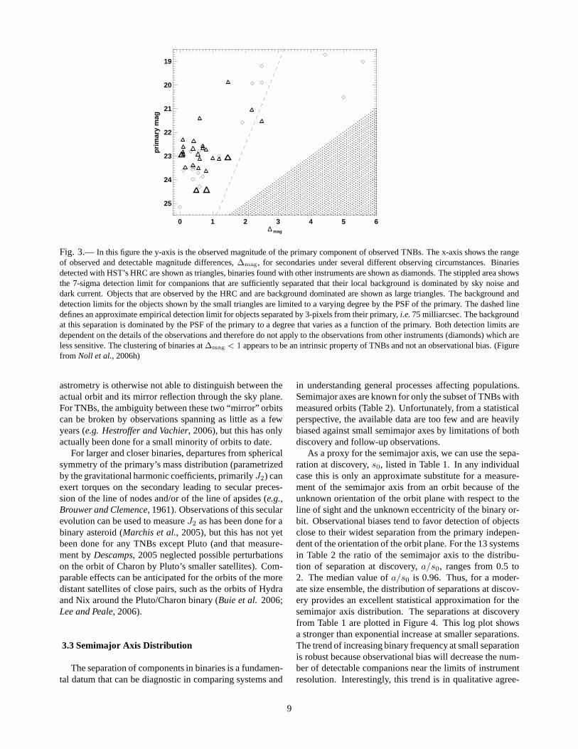
Fig. 3.— In this figure the y-axis is the observed magnitude of the primary component of observed TNBs. The x-axis shows the rangeof observed and detectable magnitude differences,∆mag, for secondaries under several different observing circumstances. Binariesdetected with HST’s HRC are shown as triangles, binaries found with other instruments are shown as diamonds. The stippled area showsthe 7-sigma detection limit for companions that are sufficiently separated that their local background is dominated by sky noise anddark current. Objects that are observed by the HRC and are background dominated are shown as large triangles. The background anddetection limits for the objects shown by the small triangles are limited to a varying degree by the PSF of the primary. Thedashed linedefines an approximate empirical detection limit for objects separated by 3-pixels from their primary,i.e.75 milliarcsec. The backgroundat this separation is dominated by the PSF of the primary to a degree that varies as a function of the primary. Both detection limits aredependent on the details of the observations and therefore do not apply to the observations from other instruments (diamonds) which areless sensitive. The clustering of binaries at∆mag < 1 appears to be an intrinsic property of TNBs and not an observational bias. (Figurefrom Noll et al., 2006h)

astrometry is otherwise not able to distinguish between theactual orbit and its mirror reflection through the sky plane.For TNBs, the ambiguity between these two “mirror” orbitscan be broken by observations spanning as little as a fewyears (e.g. Hestroffer and Vachier, 2006), but this has onlyactually been done for a small minority of orbits to date.

For larger and closer binaries, departures from sphericalsymmetry of the primary’s mass distribution (parametrizedby the gravitational harmonic coefficients, primarilyJ2) canexert torques on the secondary leading to secular preces-sion of the line of nodes and/or of the line of apsides (e.g.,Brouwer and Clemence, 1961). Observations of this secularevolution can be used to measureJ2 as has been done for abinary asteroid (Marchis et al., 2005), but this has not yetbeen done for any TNBs except Pluto (and that measure-ment byDescamps, 2005 neglected possible perturbationson the orbit of Charon by Pluto’s smaller satellites). Com-parable effects can be anticipated for the orbits of the moredistant satellites of close pairs, such as the orbits of Hydraand Nix around the Pluto/Charon binary (Buie et al.2006;Lee and Peale, 2006).

3.3 Semimajor Axis Distribution

The separation of components in binaries is a fundamen-tal datum that can be diagnostic in comparing systems and

in understanding general processes affecting populations.Semimajor axes are known for only the subset of TNBs withmeasured orbits (Table 2). Unfortunately, from a statisticalperspective, the available data are too few and are heavilybiased against small semimajor axes by limitations of bothdiscovery and follow-up observations.

As a proxy for the semimajor axis, we can use the sepa-ration at discovery,s0, listed in Table 1. In any individualcase this is only an approximate substitute for a measure-ment of the semimajor axis from an orbit because of theunknown orientation of the orbit plane with respect to theline of sight and the unknown eccentricity of the binary or-bit. Observational biases tend to favor detection of objectsclose to their widest separation from the primary indepen-dent of the orientation of the orbit plane. For the 13 systemsin Table 2 the ratio of the semimajor axis to the distribu-tion of separation at discovery,a/s0, ranges from 0.5 to2. The median value ofa/s0 is 0.96. Thus, for a moder-ate size ensemble, the distribution of separations at discov-ery provides an excellent statistical approximation for thesemimajor axis distribution. The separations at discoveryfrom Table 1 are plotted in Figure 4. This log plot showsa stronger than exponential increase at smaller separations.The trend of increasing binary frequency at small separationis robust because observational bias will decrease the num-ber of detectable companions near the limits of instrumentresolution. Interestingly, this trend is in qualitative agree-

9

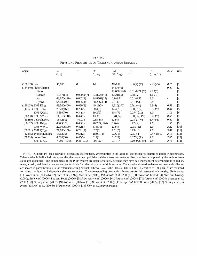
TABLE 2

PHYSICAL PROPERTIES OFTRANSNEPTUNIAN BINARIES

object a e T M pλ ρ J/J ′ refs(km) (days) (1018 kg) (g cm−3)

(136199) Eris 36,000 0 14 16,400 0.86(7) (V) 2.26(25) 0.16 [1](134340) Pluto/Charon 14,570(9) 0.40 [2]

Pluto 13,050(620) 0.51–0.71 (V) 2.03(6) [2]Charon 19,571(4) 0.00000(7) 6.387230(1) 1,521(65) 0.38 (V) 1.65(6) - [4]Nix 48,670(120) 0.002(2) 24.8562(13) 0.1–2.7 0.01–0.35 2.0 - [4]Hydra 64,780(90) 0.005(1) 38.2065(14) 0.2–4.9 0.01–0.35 2.0 - [4]

(136108) 2003 EL61 49,500(400) 0.050(3) 49.12(3) 4,210(100) 0.7(1) (v) 2.9(4) 0.53 [3](47171) 1999 TC36 7,720(460) 0.22(2) 50.4(5) 14.4(2.5) 0.08(3) (v) 0.5(3/2) 0.31 [5]

2001 QC298 3,690(70) 0.34(1) 19.2(2) 10.8(7) 0.08(V606) 1.0 1.16 [6](26308) 1998 SM165 11,310(110) 0.47(1) 130(1) 6.78(24) 0.08(3/2) (V) 0.7(3/2) 0.56 [7](65489) Ceto/Phorcys 1840(50) <0.014 9.557(8) 5.4(4) 0.08(2) (V) 1.4(6/3) 0.89 [8](66652) 1999 RZ253 4660(170) 0.46(1) 46.263(6/74) 3.7(4) 0.17(R) 1.0 1.56 [9]

1998 WW31 22,300(800) 0.82(5) 574(10) 2.7(4) 0.054(R) 1.0 2.22 [10](88611) 2001 QT297 27,880(150) 0.241(2) 825(1) 2.51(5) 0.13(r’ ) 1.0 3.41 [11](42355) Typhon/Echidna 1830(30) 0.53(2) 18.971(1) 0.96(5) 0.05(V) 0.47(18/10) 2.13 [12](58534) Logos/Zoe 8,010(80) 0.45(3) 312(3) 0.42(2) 0.37(4)(R) 1.0 2.65 [13]

2003 QY90 7,000–13,000 0.44–0.93 306–321 0.3-1.7 0.19–0.35(r’) 1.0 2.14 [14]

NOTE.—Objects are listed in order of decreasing system mass. Uncertainties in the last digit(s) of measured quantities appear in parentheses.Table entries in italics indicate quantities that have beenpublished without error estimates or that have been computed by the authors fromestimated quantities. The components of the Pluto system are listed separately because they have had independent determinations of radius,mass, albedo, and density that are not yet available for other binary or multiple systems. The wavebands used to determine geometric albedosare shown in parentheses (v is for references citing “visual” albedo,V606 is the HRC’s F606W filter). Densities of1.0 g cm−3 are assumedfor objects without an independent size measurement. The corresponding geometric albedos are for this assumed unit density. References:[1] Brown et al.(2006a,b); [2]Buie et al.(1997),Buie et al.(2006),Rabinowitz et al.(2006); [3]Brown et al.(2005); [4]Buie and Grundy(2000),Buie et al.(2006),Lee and Peale(2006); [5]Stansberry et al.(2006); [6]Margot et al.(2004); [7]Margot et al.(2004),Spencer et al.(2006); [8]Grundy et al.(2007); [9]Noll et al. (2004a); [10]Veillet et al.(2002); [11]Osip et al.(2003),Kern (2005); [12]Grundy et al., inpress; [13] Noll et al. (2004b),Margot et al.(2004); [14]Kern et al., in preparation

10

0.1 1.0Separation at Discovery (arcsec)

0

10

20

30

40

50

Cu

mu

lati

ve N

um

ber

of

TN

Bs

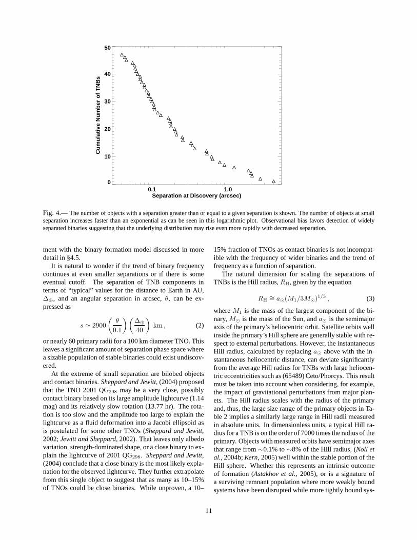
Fig. 4.—The number of objects with a separation greater than or equalto a given separation is shown. The number of objects at smallseparation increases faster than an exponential as can be seen in this logarithmic plot. Observational bias favors detection of widelyseparated binaries suggesting that the underlying distribution may rise even more rapidly with decreased separation.

ment with the binary formation model discussed in moredetail in §4.5.

It is natural to wonder if the trend of binary frequencycontinues at even smaller separations or if there is someeventual cutoff. The separation of TNB components interms of “typical” values for the distance to Earth in AU,∆⊕, and an angular separation in arcsec,θ, can be ex-pressed as

s ≃ 2900

(

θ

0.1

) (

∆⊕

40

)

km , (2)

or nearly 60 primary radii for a 100 km diameter TNO. Thisleaves a significant amount of separation phase space wherea sizable population of stable binaries could exist undiscov-ered.

At the extreme of small separation are bilobed objectsand contact binaries.Sheppard and Jewitt, (2004) proposedthat the TNO 2001 QG298 may be a very close, possiblycontact binary based on its large amplitude lightcurve (1.14mag) and its relatively slow rotation (13.77 hr). The rota-tion is too slow and the amplitude too large to explain thelightcurve as a fluid deformation into a Jacobi ellipsoid asis postulated for some other TNOs (Sheppard and Jewitt,2002;Jewitt and Sheppard, 2002). That leaves only albedovariation, strength-dominated shape, or a close binary to ex-plain the lightcurve of 2001 QG298. Sheppard and Jewitt,(2004) conclude that a close binary is the most likely expla-nation for the observed lightcurve. They further extrapolatefrom this single object to suggest that as many as 10–15%of TNOs could be close binaries. While unproven, a 10–

15% fraction of TNOs as contact binaries is not incompat-ible with the frequency of wider binaries and the trend offrequency as a function of separation.

The natural dimension for scaling the separations ofTNBs is the Hill radius,RH, given by the equation

RH∼= a⊙(M1/3M⊙)1/3 , (3)

whereM1 is the mass of the largest component of the bi-nary,M⊙ is the mass of the Sun, anda⊙ is the semimajoraxis of the primary’s heliocentric orbit. Satellite orbitswellinside the primary’s Hill sphere are generally stable with re-spect to external perturbations. However, the instantaneousHill radius, calculated by replacinga⊙ above with the in-stantaneous heliocentric distance, can deviate significantlyfrom the average Hill radius for TNBs with large heliocen-tric eccentricities such as (65489) Ceto/Phorcys. This resultmust be taken into account when considering, for example,the impact of gravitational perturbations from major plan-ets. The Hill radius scales with the radius of the primaryand, thus, the large size range of the primary objects in Ta-ble 2 implies a similarly large range in Hill radii measuredin absolute units. In dimensionless units, a typical Hill ra-dius for a TNB is on the order of 7000 times the radius of theprimary. Objects with measured orbits have semimajor axesthat range from∼0.1% to∼8% of the Hill radius, (Noll etal., 2004b;Kern, 2005) well within the stable portion of theHill sphere. Whether this represents an intrinsic outcomeof formation (Astakhov et al., 2005), or is a signature ofa surviving remnant population where more weakly boundsystems have been disrupted while more tightly bound sys-

11

tems have become even tighter in the wake of encounterswith third bodies (Petit and Mousis, 2004), or some combi-nation of the two, remains to be determined.

3.4 Mass, Albebo and Density

A particularly valuable piece of information that can bederived from the mutual orbit of a binary system is the totalmass,Msys, of the system, according to the equation

Msys =4π2a3

GT 2, (4)

wherea is the semimajor axis,G is the gravitational con-stant, andT is the orbital period. Knowledge ofa tends tobe limited by the spatial resolution of the telescope, whileknowledge ofT is limited by the timespan over whichobservations are carried out (modulo the binary orbit pe-riod). It is possible to extend the timespan of observa-tions, whereas the spatial resolution cannot generally be im-proved. Thus, typically,T is determined to much higherfractional precision thana, and the uncertainty inMsys isdominated by the uncertainty ina. Msys can often be cal-culated before all 7 elements of the binary orbit are fullydetermined, since the elementsT , a, ande are relatively in-sensitive to the ambiguity between orbits mirrored throughthe instantaneous sky plane (see §3.1).

For a system with a known mass, it is possible to deriveother parameters which offer potentially valuable composi-tional constraints. For instance, if one assumes a bulk den-sity ρ, the bulk volume of the systemVsys can be computedasVsys = Msys/ρ. How the volume and mass is partitionedbetween the two components remains unknown. Assumingthe components share the same albedo, the individual radiiof the primary and secondary can be obtained from

R1 =

(

3Vsys

4π(1 − 10−0.6∆mag)

)1/3

(5)

and equation (1) simplifies to giveR2 = R110−0.2∆mag.An effective radiusReff , equal to the radius of a sphere

having the same total surface area as the binary system canbe computed as

Reff =√

R21 + R2

2 . (6)

CombiningReff and the absolute magnitude of the sys-temHλ, one obtains the geometric albedopλ

pλ =

(

Cλ

Reff

)2

10−0.4Hλ (7)

where Cλ is a wavelength-dependent constant (Bowell,1989; Harris, 1998). For observations in the V bandCV = 664.5 km. This approach has been used to estimatealbedos for a number of TNBs by assuming their bulk den-sities must lie within a plausible range, typically taken tobe0.5 to 2 g cm−3 (e.g., Noll et al., 2004a, 2004b;Grundy et

al., 2005;Margot et al., 2005). These efforts demonstratethat the TNBs have very diverse albedos, but those albe-dos are not clearly correlated with size, color, or dynamicalclass. The calculation could also be turned around such thatan assumed range of albedos leads to a range of densities.

When the sizes of the components of a binary systemcan be obtained from an independent observation, that in-formation can be combined with the system mass to obtainthe bulk density, providing a fundamental constraint on bulkcomposition and interior structure. Sizes of TNOs are ex-tremely difficult to obtain, although a variety of methodscan be used, ranging from direct observation (e.g., Brownet al., 2004) to mutual events and stellar occultations (e.g.,Gulbis et al., 2006). For rotationally deformed bodies itis possible to constrain the density directly from the ob-served lightcurve assuming the object is able to respond asa “fluid” rubble pile (Jewitt and Sheppard, 2004;Takahashiand Ip, 2004; chapter bySheppard et al.). Spitzer SpaceTelescope observations of thermal emission have recentlyled to a number of TNO size estimates (e.g., Cruikshanket al., 2006; chapter byStansberry et al.). Unfortunately,many of the known binaries are too small and distant to bedetected at thermal infrared wavelengths by Spitzer or di-rectly resolved by HST.

Systems with density estimates include three largeTNBs: Pluto and Charon, withρ = 2.0±0.06 andρ =1.65±0.06 g cm−3, respectively (Buie et al., 2006), 2003EL61 with ρ = 3.0±0.4 g cm−3 (Rabinowitz et al., 2006),and Eris withρ = 2.26±0.25 g cm−3 (Brown, 2006). Therelatively high densities of the large TNOs are indicativeof substantial amounts of rocky and/or carbonaceous ma-terial in the interiors of these objects, quite unlike theirice-dominated surface compositions.

Four smaller TNBs have recently had their densities de-termined from Spitzer radiometric sizes. These are (26308)1998 SM165 with ρ = 0.70 ± 0.32

0.21 g cm−3 (Spencer et al.2006), (47171) 1999 TC36 with ρ = 0.5 ± 0.3

0.2 g cm−3

(Stansberry et al., 2006), (65489) Ceto/Phorcys withρ =1.38 ± 0.65

0.32 g cm−3 (Grundy et al., 2007), and (42355) Ty-phon/Echidna withρ = 0.47 ± 0.18

0.10 g cm−3 (Grundy et al.in preparation).Takahashi and Ip(2004) estimate a densityof ρ <0.7 g cm−3 for 2001 QG298. The very low densitiesof four of these five require little or no rock in their interi-ors, and even for pure H2O ice compositions, call for con-siderable void space. The higher density of Ceto/Phorcys isconsistent with a mixture of ice and rock. It is clear fromthese results that considerable diversity exists among den-sities of TNOs, but it is not yet known whether densitiescorrelate with externally observable characteristics such ascolor, lightcurve amplitude, or dynamical class.

3.5 Eccentricity Distribution and Tidal Evolution

The eccentricities of binary orbits known to date spanthe range from values near zero to a high of 0.8 (Table 2),with perhaps a clustering in the range 0.3–0.5. With the

12

usual caveats about small number statistics (N∼10), no ob-vious correlation between eccentricity and semimajor axisis present in the data obtained to date.

Keplerian two-body motion assumes point masses orbit-ing one another. The finite size of real binary componentsallows differential gravitational acceleration between nearerand more distant parts of each body to stretch them alongthe line connecting them. If their mutual orbit is eccentric,this tidal stretching varies between apoapsis and periapsis,leading to periodic flexing. The response of a body to suchflexing is characterized by the parameterQ, which is a com-plex function of interior structure and composition (Goldre-ich and Soter, 1966;Farinella et al., 1979). In a body withlow Q, tidal flexing creates more frictional heating, whichdissipates energy. A body with higherQ can flex with lessenergy dissipation. For a body having a rotation state dif-ferent from its orbital rotationQ is related to the angularlag, δ, of the tidal bulge behind the line of centers:Q−1

= tan(2δ). As with orbital eccentricity, this situation pro-duces time-variable flexing, and thus frictional heating anddissipation of energy. Typical values ofQ for rocky plan-ets and icy satellites are in the 10 to 500 range (Goldreichand Soter, 1966;Farinella et al., 1979;Dobrovolskis et al.,1997).

The energy dissipated by tidal flexing comes from or-bital and/or rotational energy, leading to changes in orbitalparameters and rotational states over time. Tides raised onthe primary tend to excite eccentricity, while tides raisedonthe secondary result in damping. The general trend is to-ward circular orbits, with both objects’ spin vectors alignedand spinning at the same rate as their orbital motion. Thetimescale for circularization of the orbit is given by

τcirc =4Q2M2

63M1

√

a3

G(M1 + M2)

(

a

R2

)5

(8)

wherea is the orbital semimajor axis,M1 is the mass ofthe primary, andM2, R2, andQ2 are the mass, radius, andQ of the secondary (e.g., Goldreich and Soter, 1966). It isimportant to recognize that this formula (a) assumes the sec-ondary to have zero rigidity, and (b) assumes that the eccen-tricity evolution due to tides raised on the primary is ignor-able. Neither of these assumptions may be justified, espe-cially in the case of near-equal sized binaries (for a thoroughdiscussion, seeGoldreich and Soter, 1966). The timescale(8) is sensitive to the ratio of the semimajor axis to thesize of the secondary. Larger and/or closer secondaries arelikely to have their orbits circularized much faster than morewidely-separated systems. For example, the close binary(65489) Ceto/Phorcys hasa = 1,840 km,M1 = 3.7×1018

kg, M2 = 1.7×1018 kg, andR2 = 67 km (Grundy et al.,2007). ForQ = 100 (a generic value for solid bodies), itsorbit should circularize on a relatively short timescale oftheorder of∼105 years. A more widely separated example,(26308) 1998 SM165 hasa = 11,300 km,M1 = 6.5×1018

kg, M2 = 2.4×1017 kg, andR2 = 48 km (Spencer et al.,2006), leading to a much longer circularization timescale

of the order of∼1010 years, consistent with the observa-tion that it still has a moderate orbital eccentricity of 0.47(Margot, 2004).

Tidal effects can also synchronize the spin rate ofthe secondary to its orbital period (as in the case of theEarth/Moon system) and, on a longer timescale, synchro-nize the primary’s spin rate as well (as for Pluto/Charon).The timescale for spin locking the primary (slowing its spinto match the mutual orbital period) is given by

τdespin,1 =Q1R

31ω1

GM1

(

M1

M2

)2 (

a

R1

)6

(9)

whereω1 is the primary’s initial angular rotation rate andR1 is its radius (Goldreich and Soter, 1966). The initialangular rotation rate is not known, but an upper limit is thebreak-up rotation rate, which is within 50 percent of 3.3hours for the 0.5 to 2 g cm−3 range of densities discussed.For (65489) Ceto/Phorcys and (26308) 1998 SM165 withprimary radii (R1) of 86 km (Grundy et al., 2007) and 147km (Spencer et al., 2006), we find the spinlock timescale tobe∼104 and∼105 years respectively, slightly faster thanthe circularization timescale. The timescale for de-spinningthe secondary,τdespin,2, is given by swapping subscripts1and2 in (9).

The general case for both tidal circularization and tidaldespinning in binaries is complex (e.g. Murray and Der-mott, 1999). Binaries in the transneptunian population in-clude many where the secondary is of comparable size tothe primary. For these systems, it is not safe to make thecommon assumption that the tide raised by the secondaryon the primary is ignorable. Furthermore, there are manysystems where the binary orbit has moderate to high eccen-tricity invalidating the simplifying assumptions possible fornearly circular orbits. A full treatment of the tidal dynam-ics for the kinds of systems we find in the transneptunianpopulation would make an interesting addition to the litera-ture. In the meantime, observation is likely to lead the wayin understanding the dynamics of these systems.

3.6 Colors and Lightcurves

The spectral properties of TNOs and their temporal vari-ation are fundamental probes of the surfaces of these ob-jects (see chapters 7-11, this volume). The colors of TNOshave long been known to be highly variable (Jewitt and Luu,1998) and some correlations of color with other physical ordynamical properties have been claimed (e.g.Peixinho etal., 2004). A natural question is whether this variabilitycan be used to constrain either the origin of TNBs, the ori-gin of color diversity, or both. For example, one can askwhether TNB components are similarly or differently col-ored. Because TNBs are thought to be primordial, differ-ences in color could be either due to mixing of different-composition populations in the protoplanetary disk beforethe bound systems were formed or different collisional andevolutionary histories of components after they are bound.

13

A handful of TNBs have reported single-epoch resolvedcolor measurements. Some of these objects are solar-colored [2000 CF105, (58534) Logos/Zoe, (47171) 1999TC36, (66652) 1999 RZ253, (88611) 2001QT297], whileothers are more gray [2001QC298, (65489) Ceto/Phorcys].However, so far, the components have colors that are consis-tent with each other within the uncertainties of the measure-ments, 0.1–0.3 mags (Margot, 2005;Noll et al., 2004a,b;Osip et al, 2003;Grundy et al., 2007). This similarity im-plies that the components are composed of similar material,at least on the surface. It also suggests that the assumptionof equal albedo and density usually made for binaries mayhave some basis in fact.

Spectra are even better composition diagnostics thancolor measurements. Separate spectra of binary compo-nents are currently available only for the Pluto/Charon pair(Buie et al., 1987; Fink and DiSanti, 1988; Buie andGrundy, 2000) and for 2003 EL61 (Barkume et al., 2006).Pluto and Charon have well known spectral differences thatmay be primarily related to the size threshold for retainingthe very volatile CH4 and N2 ices found on Pluto but not onCharon. 2003 EL61 and its larger satellite, by contrast, bothhave spectra that are dominated by water ice.

Lightcurves are diagnostic of both compositional vari-ation on surfaces and of non-spherical shapes. They alsogive rotation rates. In binary systems, the rotation state ofthe components is subject to tidal evolution (see §3.5). Bothunresolved and resolved lightcurves can be useful for ad-dressing these issues.

Unresolved lightcurves of short duration for a number ofTNBs have been obtained, sometimes with incomplete orinconsistent results. Lightcurves of (47171) 1999 TC36 and(42355) Typhon/Echidna showed variations on the order of0.10–0.15 mags, but no period was determinable from thedata (Ortiz et al., 2003). Similarly, observations of (66652)1999 RZ253 and 2001 QC298 showed small amplitude, butnon-systematic variation over a 4–6 hour duration (Kern,2005).Romanishin et al.(2001) reported a lightcuve for theunresolved binary (26308) 1998 SM165, obtained from the1.8m Vatican Advanced Technology Telescope in 1999 and2000, with a moderate amplitude of 0.56 mags. The periodwas determined to be either 3.983 hours (single-peaked,caused by an albedo spot) or 7.966 hours (double-peaked,caused by nonspherical shape). The single-peaked period isnear the break-up period ( 3.3 hours) for a solid ice body.Because the unresolved lightcurve of (26308) 1998 SM165

did not show any color variation with timeRomanishin etal. argued for the longer, double-peaked period as the mostlikely. Lightcurve measurements of the same binary madeat Lowell Observatory in 2006 found a slightly longer pe-riod of 8.40±0.05 hours (Spencer et al., 2006).

Resolved ground based lightcurves of binaries are chal-lenging and can only be obtained under excellent condi-tions at a few facilities, and only for objects with the widestseparations. Discovery observations of the binary (88611)2001 QT297 at Las Campanas Observatory with Magellanrevealed brightness changes in the secondary component of

0.3 mag in 30 minutes (Osip et al., 2003). Follow-up ob-servations revealed the secondary to have a single-peakedperiod of 5–7 hours while the magnitude of the primaryremained constant. Additional resolved color lightcurvemeasurements found the two surfaces to share similar col-ors throughout the rotation indicating homogeneous, simi-lar surfaces (Kern, 2005). Similar observations showed thatboth components of 2003 QY90 to be variable. The pri-mary and secondary components were observed to changeby 0.34±0.12 and 0.9±0.36 mags, respectively, over sixhours of observation (Kern and Elliot, 2006). The largeamplitude of the secondary component sometimes results inthe secondary being brighter than the primary. Both com-ponents of the wide binary 2005 EO304 are variable withvariations on the order of 0.3 mags over a period of 4 hours(Kern, 2005).

Space based observations from HST resolve the compo-nents of binaries and can constrain the variability of com-ponents in these systems. The best studied system, by far,is the Pluto/Charon binary where detailed lightcurve mea-surements have been made (Buie et al., 1997). TNBs thathave had their orbits measured by HST have multiple-epochphotometric measurements, although frequently the tempo-ral sampling is poor. (58534) Logos/Zoe shows variabilityin the primary of at least∼ 0.8 mag, making it challeng-ing at times to distinguish the primary from the secondary(Noll et al., 2004). However, with only a few widely spacedsamples, this remains, for the moment, only an intriguingsuggestion of a lightcurve. Three objects, (47171) 1999TC36, 2001 QC298 and (65489) Ceto/Phorcys have virtuallyno variation in flux, implying they may be relatively spher-ical, homogeneous, and/or pole-on (although we note thecontradictory ground-based observations of (47171) 1999TC36). Once again, the sampling density is far to small toallow anything more than informed speculation.

3.7 Orbit Plane and Mutual Events

The tremendous scientific benefit that can derive frommutual occultations or eclipses between a poorly-resolvedobject and its satellite was abundantly illustrated by the se-ries of mutual events between Pluto and Charon during the1980s (Binzel and Hubbard, 1997). As discussed before,these events enabled measurement of the sizes and albedosof both objects, of their distinct surface compositions, andeven of albedo patterns on their surfaces.

For observable mutual events to happen either the ob-server or the Sun (or both) must be temporarily aligned witha TNB’s orbit plane. An “occultation-type” event occurswhen one component of the TNB passes in front of, andfully or partially occults, the other component from the ob-server’s point of view. An “eclipse-type” event takes placewhen the TNB components are aligned with the Sun andthe shadow of one falls on the other. Because the Sun andEarth have nearly equal lines of sight to TNBs, most mu-tual events observable from the Earth are combinations ofoccultation-type and eclipse-type events.

14

The larger the objects are compared with their separa-tion, the farther the orbit plane can deviate from either ofthese two types of alignments and still produce an observ-able mutual event. The criteria for both types of events canbe expressed asR1 + R2 > s sin(φ) whereR1 andR2

are previously defined and,s is their separation during aconjunction (equal to the semimajor axis, for the case of acircular orbit), andφ is the angle between the observer orthe Sun and the plane of the binary orbit. During any con-junction when either criterion is satisfied, a mutual eventcan be observed. The period during which the orbit plane isaligned closely enough to the Sun’s or to the Earth’s line ofsight to satisfy the criteria for events can be thought of as amutual event season.

Each orbit of a transneptunian secondary brings a su-perior conjunction (when the primary is closer to the ob-server) and an inferior conjunction (when the secondary iscloser), so shorter orbital periods lead to more frequent con-junctions and associated opportunities for mutual events.The most recent mutual event season of Pluto and Charonlasted from 1985 through 1990, and, since their mutual or-bit period is only 6.4 days, there were hundreds of observ-able events during that season. For more widely separated,smaller pairs, with longer orbital periods, the mutual eventseasons may be shorter and conjunctions may be less fre-quent, leading to far fewer observable events, or even noneat all. For example, (26308) 1998 SM165 has a reasonablywell-determined orbit with a period of 130 days, a semima-jor axis of 11,170 km , and an eccentricity of 0.47 (Margot,2004). From Spitzer thermal observations, the diameters ofthe primary and secondary bodies are estimated to be 294and 96 km, respectively (Spencer et al., 2006). Ignoring un-certainties in the current orbital elements, the mutual eventseason will last from 2020 through 2026, with 12 mutualevents being observable at solar elongations of 90 degreesor more. Of these 12 events, 2 are purely occultation-typeevents and one is purely an eclipse-type event. The rest in-volve combinations of both occultation and eclipse.

4. BINARY FORMATION

When the Pluto/Charon binary was the only example ofa true binary in the solar system (true binary≡ two objectsorbiting a barycenter located outside either body) it couldbe discounted as just another of the peculiarities associatedwith this yet-to-be-dwarf planet. The discovery of numer-ous similar systems among TNOs, however, has changedthis calculus. Any successful model for producing TNBscannot rely on low-probability events, but must instead em-ploy processes that were commonplace in the portion of thepreplanetary nebula where these objects were formed. For-mation models must also account for the observed prop-erties of TNBs including the prevalence of similar-size bi-naries, the range of orbital eccentricities, and the steeplyincreasing fraction of binaries at small angular separations.Survival of binaries, once they are formed, is another impor-

tant factor that must be considered when, for instance, com-paring the fraction of binaries found in different dynamicalpopulations or their distribution as a fraction of Hill radius.

Several possible modes for the formation of solar sys-tem binaries have been discussed in the literature includ-ing fission, dynamical capture, and collision (c.f. reviews byRichardson and Walsh, 2006; Dobrovolskis et al., 1997).For TNOs, capture and/or collision models have been themost thoroughly investigated. Fission is unlikely to be im-portant for objects as large as the currently known TNBs.Other possible mechanisms for producing binaries,e.g.volatile-driven splitting, as is observed in comets, have notbeen explored. Interestingly, both capture and collisionalformation models share the requirement that the numberof objects in the primordial Kuiper Belt (at least the smallones) be at least a couple of orders of magnitude higher thancurrently found in transneptunian space. It follows that allof the TNBs observed today are primordial.

4.1 Capture

Capture models rely, in one form or another, on three-body interactions to remove angular momentum and pro-duce a bound pair. As we show in detail below in §4.5, theyare also very sensitive to the assumed velocity distributionof planetesimals.Goldreich et al.(2002, hereafterG02) de-scribed two variations of the three-body model,L3, involv-ing three discrete bodies, andL2s, where the third body isreplaced by a dynamical drag coefficient corresponding to a“sea” of weakly interacting smaller bodies. InG02’sanaly-sis, theL2s channel was more efficient at forming binariesby roughly an order of magnitude.

Astakhov et al.(2005) extended the capture model byexploring how a weakly and temporarily bound (a ∼ RH)pair of big bodies hardens when a third small body (“in-truder”) passes within the Hill radius (3), of the pair. Theircalculations assume the existence of transitory binaries thatcan complete up to∼10 mutual orbits before the third bodyapproaches. They find that a binary hardens most effec-tively when the intruder mass is a few percent that of a bigbody (this result likely depends on their assumed approachvelocities of up to5vH wherevH ≡ ΩKRH is the Hill ve-locity, with ΩK ≃ 2π/(200 yr) denoting the local Keplerfrequency).

The two capture formation channelsL3 andL2s requirethat binaries form—and formation times increase with de-creasing separationa—beforev > vH. Given the pre-ponderance of classical binaries (Stephens and Noll, 2006;Fig.), we can speculate that the primordial classical beltmay have enjoyed dynamically cold (sub-Hill or marginallyHill) conditions for a longer duration than the primordialscattered population.

Dynamical capture is the only viable formation scenariofor many TNBs with high angular momentum (§4.4) andis a possible formation scenario for most, if not all, knownTNBs. Given the apparent importance of capture models,

15

we explore them in detail in §4.5 with a specific focus onthe case of binaries with similar mass components.

4.2 Collision

Collisional models were proposed for the Pluto/Charonbinary early on based on the angular momentum of thesystem (McKinnon, 1984, 1989) and one such model hasrecently been shown to be numerically feasible (Canup,2005). However, as we note below, angular momentum ar-guments alone are not sufficient to prove an impact origin.Nix and Hydra, the outermost satellites of Pluto, plausiblyresulted from the same impact that generated Charon (Sternet al., 2006). Ward and Canup(2006) propose that colli-sional debris within the exterior 4:1 and 6:1 resonances ofCharon—resonances stabilized by Charon’s initially largeeccentricity—accumulated to form Nix and Hydra. Accord-ing to their scenario, as Charon’s orbit tidally expanded, thesmall satellites would have been forced outwards to theircurrent locations in resonant lockstep with Charon. Tidalcircularization of Charon’s orbit would have eventually re-leased Nix and Hydra from resonance. In this scenario, thenearly circular orbits of Nix and Hydra result from theircoalescence from a dissipative, nearly circular disk; theireccentricities are not altered by resonant migration becausethe resonances involved are of the co-rotation type.

The small satellites of Pluto-sized TNOs 2003 EL61 and(136199) Eris, characterized by satellite-to-primary massratios of∼1%, might also have formed by impacts (Stern,2002). Some collisional simulations (Durda et al., 2004;Canup, 2005) reproduce such low mass ratios. Tidal expan-sion of satellite orbits can explain, to within factors of a few,the current semimajor axes of the companions of 2003 EL61

(Brown et al.2005a). An unresolved issue is the origin ofthe small, but significant, orbital eccentricity,0.05± 0.003,for the outermost satellite of 2003 EL61. Tides should havereduced the eccentricity to values much smaller. Also themutual orbital inclination of the satellites of 2003 EL61,which might be as large as39 (Brown et al.2006a), has yetto be explained. Formation by collisionless capture alongthe lines ofG02, though not ruled out, remains poorly ex-plored for unequal mass components (Brown et al.2005a).

To occur with reasonable frequency, collisions betweenPluto-sized (R ∼ 1000 km) TNOs must be gravitationallyfocused. Transneptunian space may have been populated bya few dozen such objects (Kenyon and Luu1999). If theirrelative velocities were less than the Hill velocity,vH, thenthe collision timescale would be∼6 Myr (18). Otherwisethe collision time exceeds∼500 Myr. Like collisionlesscapture (see §4.1), binary formation by giant impacts musthave taken place while the disk was dynamically cold.

4.3 Hybrids

Hybrid collision/capture models are possible as well;two variants on this theme have been proposed.

Weidenschilling(2002) considered a model in whicha third big body collides with one member of the scat-tering pair. Since physical collisions have smaller cross-sections than gravitational interactions, this mechanismre-quires∼102 more big (R ∼ 100 km) bodies than are cur-rently observed to operate at the same rate asL3. It alsopredicts an unobserved prevalence of widely separated bi-naries.

Funato et al. (2004) proposed that observed binariesform by the exchange reactionLs+ L → L2 + s wherein asmall body of massMsm, originally orbiting a big body ofmassMbig, is ejected by a second big body. In the majorityof ejections, the small body’s energy increases by its orbitalbinding energy∼Msmv2

esc/2, leaving the big bodies boundwith separationa ∼ (Mbig/Msm)R. As formulated, thismodel predicts a prevalence of very high eccentricity bina-ries that is not observed. The rate-limiting step for the ex-change reaction model is the formation of the pre-existing(Ls) binary, which requires two big bodies to collide andfragment (18).

4.4 Angular Momentum

It is possible, in some cases, to distinguish between cap-ture and collision based on the angular momentum of thebinary. Early theoretical arguments in favor of a collisionalorigin for Pluto/Charon were based on the fact that the totalangular momentum of the system exceeds breakup for a sin-gle, reconstituted object (e.g. McKinnon, 1989). However,it can also be shown that to have formed from a fragmen-tary collision, binary components cannot have too muchangular momentum. It is conventional to express angu-lar momentum asJ/J ′, where the combined orbital andspin angular momentum of the binaryJ is normalized byJ ′ =

√

GM3totReff , whereG is the gravitational constant,

Mtot is the total system mass, andReff is the radius ofan equivalent spherical object containing the total systemmass. Canup(2005) found that binary systems producedby single collisions haveJ/J ′ < 0.8 (for an order-of-magnitude derivation of this result, seeChiang et al., 2006).For instance, the Earth/Moon system hasJ/J ′ ≃ 0.1 andthe Pluto/Charon system hasJ/J ′ ≃ 0.4.

In Table 2, we listJ/J ′ for TNBs. We use actual mea-surements where they exist, otherwise the calculation as-sumes that both binary components have spin periods of 8hours and densities of 1 g cm−3. For about half of the TNBsdocumented in Table 2,J/J ′ exceeds unity, so much angu-lar momentum that formation via two-body collisions canbe ruled out.

4.5 Detailed Capture Models

Capture models are of particular importance for TNBsas the only class of models that can explain the existence ofhigh angular momentum systems. We review and expand,in detail, on capture models in this section.

16

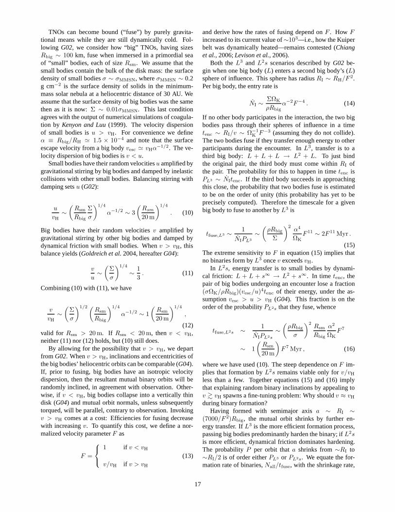
TNOs can become bound (“fuse”) by purely gravita-tional means while they are still dynamically cold. Fol-lowing G02, we consider how “big” TNOs, having sizesRbig ∼ 100 km, fuse when immersed in a primordial seaof “small” bodies, each of sizeRsm. We assume that thesmall bodies contain the bulk of the disk mass: the surfacedensity of small bodiesσ ∼ σMMSN, whereσMMSN ∼ 0.2g cm−2 is the surface density of solids in the minimum-mass solar nebula at a heliocentric distance of 30 AU. Weassume that the surface density of big bodies was the samethen as it is now:Σ ∼ 0.01σMMSN. This last conditionagrees with the output of numerical simulations of coagula-tion by Kenyon and Luu(1999). The velocity dispersionof small bodies isu > vH. For convenience we defineα ≡ Rbig/RH ≃ 1.5 × 10−4 and note that the surfaceescape velocity from a big bodyvesc ≃ vHα−1/2. The ve-locity dispersion of big bodies isv < u.

Small bodies have their random velocitiesu amplified bygravitational stirring by big bodies and damped by inelasticcollisions with other small bodies. Balancing stirring withdamping setsu (G02):

u

vH

∼

(

Rsm

Rbig

Σ

σ

)1/4

α−1/2 ∼ 3

(

Rsm

20 m

)1/4

. (10)

Big bodies have their random velocitiesv amplified bygravitational stirring by other big bodies and damped bydynamical friction with small bodies. Whenv > vH, thisbalance yields (Goldreich et al.2004, hereafterG04):

v

u∼

(

Σ

σ

)1/4

∼1

3. (11)

Combining (10) with (11), we have

v

vH

∼

(

Σ

σ

)1/2 (

Rsm

Rbig

)1/4

α−1/2 ∼ 1

(

Rsm

20 m

)1/4

,

(12)valid for Rsm > 20 m. If Rsm < 20 m, thenv < vH,neither (11) nor (12) holds, but (10) still does.

By allowing for the possibility thatv > vH, we departfrom G02. Whenv > vH, inclinations and eccentricities ofthe big bodies’ heliocentric orbits can be comparable (G04).If, prior to fusing, big bodies have an isotropic velocitydispersion, then the resultant mutual binary orbits will berandomly inclined, in agreement with observation. Other-wise, if v < vH, big bodies collapse into a vertically thindisk (G04) and mutual orbit normals, unless subsequentlytorqued, will be parallel, contrary to observation. Invokingv > vH comes at a cost: Efficiencies for fusing decreasewith increasingv. To quantify this cost, we define a nor-malized velocity parameterF as

F =

1 if v < vH

v/vH if v > vH

(13)

and derive how the rates of fusing depend onF . How Fincreased to its current value of∼103—i.e., how the Kuiperbelt was dynamically heated—remains contested (Chianget al., 2006;Levison et al., 2006).

Both theL3 and L2s scenarios described byG02 be-gin when one big body (L) enters a second big body’s (L)sphere of influence. This sphere has radiusRI ∼ RH/F 2.Per big body, the entry rate is

NI ∼ΣΩK

ρRbig

α−2F−4 . (14)

If no other body participates in the interaction, the two bigbodies pass through their spheres of influence in a timetenc ∼ RI/v ∼ Ω−1

K F−3 (assuming they do not collide).The two bodies fuse if they transfer enough energy to otherparticipants during the encounter. InL3, transfer is to athird big body: L + L + L → L2 + L. To just bindthe original pair, the third body must come withinRI ofthe pair. The probability for this to happen in timetenc isPL3 ∼ NItenc. If the third body succeeds in approachingthis close, the probability that two bodies fuse is estimatedto be on the order of unity (this probability has yet to beprecisely computed). Therefore the timescale for a givenbig body to fuse to another byL3 is

tfuse,L3 ∼1

NIPL3

∼

(

ρRbig

Σ

)2α4

ΩK

F 11 ∼ 2F 11 Myr .

(15)The extreme sensitivity toF in equation (15) implies thatno binaries form byL3 oncev exceedsvH.

In L2s, energy transfer is to small bodies by dynami-cal friction: L + L + s∞ → L2 + s∞. In time tenc, thepair of big bodies undergoing an encounter lose a fraction(σΩK/ρRbig)(vesc/u)4tenc of their energy, under the as-sumptionvesc > u > vH (G04). This fraction is on theorder of the probabilityPL2s that they fuse, whence

tfuse,L2s ∼1

NIPL2s

∼

(

ρRbig

σ

)2Rsm

Rbig

α2

ΩK

F 7

∼ 1

(

Rsm

20 m

)

F 7 Myr , (16)

where we have used (10). The steep dependence onF im-plies that formation byL2s remains viable only forv/vH

less than a few. Together equations (15) and (16) implythat explaining random binary inclinations by appealing tov & vH spawns a fine-tuning problem: Why shouldv ≈ vH

during binary formation?Having formed with semimajor axisa ∼ RI ∼

(7000/F 2)Rbig, the mutual orbit shrinks by further en-ergy transfer. IfL3 is the more efficient formation process,passing big bodies predominantly harden the binary; ifL2sis more efficient, dynamical friction dominates hardening.The probabilityP per orbit thata shrinks from∼RI to∼RI/2 is of order eitherPL3 or PL2s. We equate the for-mation rate of binaries,Nall/tfuse, with the shrinkage rate,

17

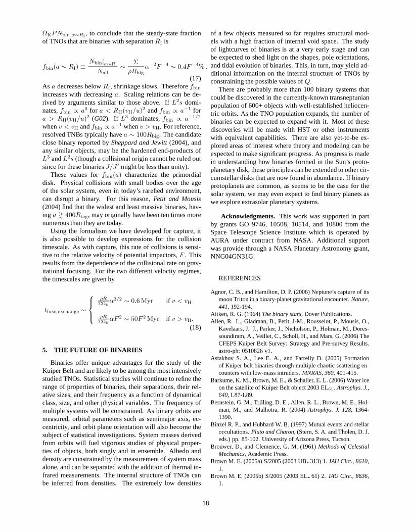
ΩKPNbin|x∼RI, to conclude that the steady-state fraction

of TNOs that are binaries with separationRI is

fbin(a ∼ RI) ≡Nbin|a∼RI

Nall

∼Σ

ρRbig

α−2F−4 ∼ 0.4F−4% .

(17)As a decreases belowRI, shrinkage slows. Thereforefbin

increases with decreasinga. Scaling relations can be de-rived by arguments similar to those above. IfL2s domi-nates,fbin ∝ a0 for a < RH(vH/u)2 andfbin ∝ a−1 fora > RH(vH/u)2 (G02). If L3 dominates,fbin ∝ a−1/2

whenv < vH andfbin ∝ a−1 whenv > vH. For reference,resolved TNBs typically havea ∼ 100Rbig. The candidateclose binary reported bySheppard and Jewitt(2004), andany similar objects, may be the hardened end-products ofL3 andL2s (though a collisional origin cannot be ruled outsince for these binariesJ/J ′ might be less than unity).

These values forfbin(a) characterize the primordialdisk. Physical collisions with small bodies over the ageof the solar system, even in today’s rarefied environment,can disrupt a binary. For this reason,Petit and Mousis(2004) find that the widest and least massive binaries, hav-ing a & 400Rbig, may originally have been ten times morenumerous than they are today.

Using the formalism we have developed for capture, itis also possible to develop expressions for the collisiontimescale. As with capture, this rate of collisions is sensi-tive to the relative velocity of potential impactors,F . Thisresults from the dependence of the collisional rate on grav-itational focusing. For the two different velocity regimes,the timescales are given by

tfuse,exchange ∼

ρRΣΩk

α3/2 ∼ 0.6 Myr if v < vH

ρRΣΩk

αF 2 ∼ 50F 2 Myr if v > vH.(18)

5. THE FUTURE OF BINARIES

Binaries offer unique advantages for the study of theKuiper Belt and are likely to be among the most intensivelystudied TNOs. Statistical studies will continue to refine therange of properties of binaries, their separations, their rel-ative sizes, and their frequency as a function of dynamicalclass, size, and other physical variables. The frequency ofmultiple systems will be constrained. As binary orbits aremeasured, orbital parameters such as semimajor axis, ec-centricity, and orbit plane orientation will also become thesubject of statistical investigations. System masses derivedfrom orbits will fuel vigorous studies of physical proper-ties of objects, both singly and in ensemble. Albedo anddensity are constrained by the measurement of system massalone, and can be separated with the addition of thermal in-frared measurements. The internal structure of TNOs canbe inferred from densities. The extremely low densities

of a few objects measured so far requires structural mod-els with a high fraction of internal void space. The studyof lightcurves of binaries is at a very early stage and canbe expected to shed light on the shapes, pole orientations,and tidal evolution of binaries. This, in turn, may yield ad-ditional information on the internal structure of TNOs byconstraining the possible values ofQ.

There are probably more than 100 binary systems thatcould be discovered in the currently-known transneptunianpopulation of 600+ objects with well-established heliocen-tric orbits. As the TNO population expands, the number ofbinaries can be expected to expand with it. Most of thesediscoveries will be made with HST or other instrumentswith equivalent capabilities. There are also yet-to-be ex-plored areas of interest where theory and modeling can beexpected to make significant progress. As progress is madein understanding how binaries formed in the Sun’s proto-planetary disk, these principles can be extended to other cir-cumstellar disks that are now found in abundance. If binaryprotoplanets are common, as seems to be the case for thesolar system, we may even expect to find binary planets aswe explore extrasolar planetary systems.

Acknowledgments. This work was supported in partby grants GO 9746, 10508, 10514, and 10800 from theSpace Telescope Science Institute which is operated byAURA under contract from NASA. Additional supportwas provide through a NASA Planetary Astronomy grant,NNG04GN31G.

REFERENCES

Agnor, C. B., and Hamilton, D. P. (2006) Neptune’s capture ofitsmoon Triton in a binary-planet gravitational encounter.Nature,441, 192-194.

Aitken, R. G. (1964)The binary stars, Dover Publications.Allen, R. L., Gladman, B., Petit, J-M., Rousselot, P., Mousis, O.,

Kavelaars, J. J., Parker, J., Nicholson, P., Holman, M., Dores-soundiram, A., Veillet, C., Scholl, H., and Mars, G. (2006) TheCFEPS Kuiper Belt Survey: Strategy and Pre-survey Results.astro-ph: 0510826 v1.

Astakhov S. A., Lee E. A., and Farrelly D. (2005) Formationof Kuiper-belt binaries through multiple chaotic scattering en-counters with low-mass intruders.MNRAS, 360, 401-415.

Barkume, K. M., Brown, M. E., & Schaller, E. L. (2006) Water iceon the satellite of Kuiper Belt object 2003 EL61. Astrophys. J.,640, L87-L89.

Bernstein, G. M., Trilling, D. E., Allen, R. L., Brown, M. E.,Hol-man, M., and Malhotra, R. (2004)Astrophys. J. 128, 1364-1390.

Binzel R. P., and Hubbard W. B. (1997) Mutual events and stellaroccultations.Pluto and Charon, (Stern, S. A. and Tholen, D. J.eds.) pp. 85-102. University of Arizona Press, Tucson.

Brouwer, D., and Clemence, G. M. (1961)Methods of CelestialMechanics, Academic Press.

Brown M. E. (2005a) S/2005 (2003 UB313) 1.IAU Circ., 8610,1.

Brown M. E. (2005b) S/2005 (2003 EL61) 2. IAU Circ., 8636,1.

18

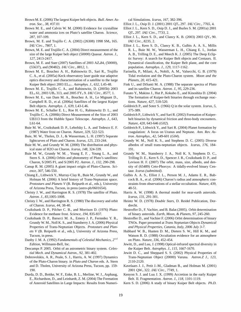
Brown M. E. (2006) The largest Kuiper belt objects.Bull. Amer. As-tron. Soc., 38, #37.01

Brown M. E., and Calvin W. M. (2000) Evidence for crystallinewater and ammonia ices on Pluto’s satellite Charon.Science,287, 107-109.

Brown, M. E. and Trujillo C. A. (2002) (26308) 1998 SM165.IAU Circ., 7807, 1.

Brown, M. E. and Trujillo C. A. (2004) Direct measurement of thesize of the large Kuiper belt object (50000) Quaoar.Astron. J.,127, 2413-2417.

Brown, M. E. and Suer (2007) Satellites of 2003 AZ84, (50000),(55637), and (90482).IAU Circ., 8812, 1.

Brown M. E., Bouchez A. H., Rabinowitz D., Sari R., TrujilloC. A., et al. (2005a) Keck observatory laser guide star adaptiveoptics discovery and characterization of a satellite to thelargeKuiper Belt object 2003 EL61. Astrophys. J., 632, L45-48.

Brown M. E., Trujillo C. A., and Rabinowitz, D. (2005b) 2003EL 61, 2003 UB 313, and 2005 FY9. IAU Circ., 8577, 1.

Brown M. E., van Dam M. A., Bouchez A. H., Le Mignant D.,Campbell R. D., et al. (2006a) Satellites of the largest KuiperBelt objects.Astrophys. J., 639, L43-L46.

Brown M. E., Schaller E. L., Roe H. G., Rabinowitz D. L., andTrujillo C. A. (2006b) Direct Measurement of the Size of 2003UB313 from the Hubble Space Telescope.Astrophys. J., 643,L61-64.

Buie M. W., Cruikshank D. P., Lebofsky L. A. and Tedesco E. F.(1987) Water frost on Charon.Nature, 329,522-523.

Buie, M. W., Tholen, D. J., & Wasserman, L. H. (1997) Separatelightcurves of Pluto and Charon.Icarus, 125, 233-244.

Buie M. W., and Grundy W. M. (2000) The distribution and phys-ical state of H2O on Charon.Icarus, 148,324-339.

Buie M. W., Grundy W. M. , Young E. F. , Young L. A., andStern S. A. (2006) Orbits and photometry of Pluto’s satellites:Charon, S/2005 P1, and S/2005 P2.Astron. J., 132, 290-298.

Canup R. M. (2005) A giant impact origin of Pluto-Charon.Sci-ence, 307,546-550.

Chiang E., Lithwick Y., Murray-Clay R., Buie M., Grundy W., andHolman M. (2006) A brief history of Trans-Neptunian space.Protostars and Planets V(B. Reipurth et al., eds.), Universityof Arizona Press, Tucson, in press (astro-ph/0601654).

Christy J. W., and Harrington R. S. (1978) The satellite of Pluto.Astron. J., 83,1005-1008.

Christy J. W., and Harrington R. S. (1980) The discovery and orbitof Charon.Icarus, 44,38-40.

Cruikshank D. P., Pilcher C. B., and Morrison D. (1976) Pluto:Evidence for methane frost.Science, 194,835-837.

Cruikshank D. P., Barucci M. A., Emery J. P., Fernndez Y. R.,Grundy W. M., Noll K. S., and Stansberry J. A. (2006) PhysicalProperties of Trans-Neptunian Objects.Protostars and Plan-ets V (B. Reipurth et al., eds.), University of Arizona Press,Tucson, in press.

Danby J. M. A. (1992)Fundamentals of Celestial Mechanics, 2nd

Edition, Willmann-Bell, Inc.Descamps P. 2005. Orbit of an astrometric binary system.Celes-

tial Mech. and Dynamical Astron., 92,381-402.Dobrovolskis, A. R., Peale, S. J., Harris, A. W. (1997) Dynamics

of the Pluto-Charon binary. inPluto and Charoneds. A. Sternand D. Tholen, University of Arizona Press, Tucson, pp. 159-190.

Durda, D. D., Bottke, W. F., Enke, B. L., Merline, W. J., Asphaug,E., Richardson, D., and Leinhardt, Z. M. (2004) The Formationof Asteroid Satellites in Large Impacts: Results from Numeri-

cal Simulations.Icarus, 167, 382-396.Elliot J. L., Osip D. J. (2001) 2001 QT297. IAU Circ., 7765, 4.Elliot J. L., Kern S. D., Osip D. J., and Burles S. M. (2001a) 2001

QT 297. IAU Circ., 7733, 2.Elliot J. L., Kern S. D., and Clancy K. B. (2003) 2003 QY90.

IAU Circ., 8235, 2.Elliot J. L., Kern S. D., Clancy K. B., Gulbis A. A. S., Millis

R. L., Buie M. W., Wasserman L. H., Chiang E. I., JordanA. B., Trilling D. E., and Meech K. J. (2005) The Deep Eclip-tic Survey: A search for Kuiper Belt objects and Centaurs. II.Dynamical classification, the Kuiper Belt plane, and the corepopulation.Astrophys. J., 129, 1117-1162.

Farinella, P., Milani, A., Nobili, A. M., Valsecchi, G. B. (1979)Tidal evolution and the Pluto-Charon system.Moon and thePlanets, 20, 415-421.

Fink U., and DiSanti M. A. (1988) The separate spectra of Plutoand its satellite Charon.Astron. J., 95,229-236.

Funato Y., Makino J., Hut P., Kokubo E., and Kinoshita D. (2004)The formation of Kuiper-belt binaries through exchange reac-tions.Nature, 427, 518-520.

Goldreich P., and Soter S. (1966) Q in the solar system.Icarus, 5,375-389.

Goldreich P., Lithwick Y., and Sari R. (2002) Formation of Kuiper-belt binaries by dynamical friction and three-body encounters.Nature, 420, 643-646 (G02).

Goldreich P., Lithwick Y., and Sari R. (2004) Planet formation bycoagulation: A focus on Uranus and Neptune.Ann. Rev. As-tron. Astrophys., 42, 549-601 (G04).

Grundy W. M., Noll K. S., and Stephens D. C. (2005) Diversealbedos of small trans-neptunian objects.Icarus, 176, 184-191.

Grundy W. M., Stansberry J. A., Noll K. S, Stephens D. C.,Trilling D. E., Kern S. D., Spencer J. R., Cruikshank D. P., andLevison H. F. (2007) The orbit, mass, size, albedo, and den-sity of (65489) Ceto-Phorcys: A tidally-evolved binary Cen-taur. Icarus (submitted).

Gulbis A. A. S., Elliot J. L., Person M. J., Adams E. R., Bab-cock B. A., et al. (2006) Charon’s radius and atmospheric con-straints from observations of a stellar occultation.Nature, 439,48-51.

Harris A. W. (1998) A thermal model for near-earth asteroids.Icarus, 131, 291-301.

Heintz W. D. (1978)Double Stars, D. Reidel Publication, Dor-drecht.

Hestroffer D., F. Vachier, and B. Balat (2005). Orbit determinationof binary asteroids.Earth, Moon, & Planets, 97, 245-260.

Hestroffer D., and Vachier F. (2006) Orbit determination ofbinaryTNOs. Paper presented atTrans Neptunian Objects Dynamicaland Physical Properties, Catania, Italy, 2006 July 3-7.

Hubbard W. B., Hunten D. M., Dieters S. W., Hill K. M., andWatson R. D. (1988) Occultation evidence for an atmosphereon Pluto.Nature, 336, 452-454.

Jewitt, D., and Luu, J. (1998) Optical-infrared spectral diversity inthe Kuiper Belt.Astrophys. J., 115, 1667-1670.

Jewitt D. C., and Sheppard S. S. (2002) Physical Properties ofTrans-Neptunian Object (20000) Varuna.Astron.Z J., 123,2110-2120.

Kavelaars J. J., Petit J.-M., Gladman B., and Holman M. (2001)2001 QW 322. IAU Circ., 7749, 1.

Kenyon S. J. and Luu J. X. (1999) Accretion in the early KuiperBelt. II. Fragmentation.Astron. J., 118, 1101-1119.

Kern S. D. (2006) A study of binary Kuiper Belt objects.Ph.D.

19

ThesisMassachussetts Institute of Technology, Boston.Kern S. D., and Elliot J. L. (2005) 2005 EO304. IAU Circ., 8526,

2.Kern S. D., and Elliot J. L. (2006) The frequency of binary Kuiper

Belt objects.Astrophys. J., 643, L57-L60.Lee M. H., and Peale S. J. (2006) On the orbits and masses of the

satellites of the Pluto-Charon system.Icarus, 184, 573-583.Levison, H. F., and Stern, S. A. (2001) On the size dependence

of the inclination distribution of the main Kuiper Belt.Icarus,121, 1730-1735.

Levison H. F., Morbidelli A., Gomes R., and Backman D. (2006)Planet migration in planetesimal disks.Protostars and Plan-ets V (B. Reipurth et al., eds.), University of Arizona Press,Tucson, in press.

Marchis F., Hestroffer D., Descamps P., Berthier J., Laver C., andde Pater I. (2005) Mass and density of asteroid 121 Hermionefrom an analysis of its companion orbit.Icarus, 178,450-464.

Margot, J. L., Brown, M. E., (2003) A Low-Density M-type As-teroid in the Main Belt.Science, 300, 1939-1942.

Margot J. L. (2004) Binary Minor Planets.Urey Prize Lecturepresented at DPS/AAS meeting 2004 November 9, Louisville,KY.

Margot, J. L., Brown, M. E., Trujillo, C. A., and Sari, R. (2004)HST observations of Kuiper Belt binariesBulletin of the Amer-ican Astronomical Society, 36, 1081.

Margot J. L., Brown, M. E., Trujillo, C. A., Sari, R., Stansberry, J.A. (2005) Kuiper Belt Binaries: Masses, Colors, and a DensityBulletin of the American Astronomical Society, 37, 737.

McKinnon, W. B. (1984) On the Origin of Triton and Pluto.Na-ture, 311, 355-358.

McKinnon, W. B. (1989) On the Origin of the Pluto-Charon Bi-nary.Astrophys. J., 344, L41-L44.

Merline W. J., Weidenschilling S. J., Durda D. D., Margot J. L.,Pravec P., and Storrs A. D. (2002) Asteroidsdohave satellites.Asteroids III (Bottke W F. Jr., Cellino A., Paolicchi P., andBinzel R. P. eds.) pp. 289-312. University of Arizona Press,Tucson.

Millis R. L., and Clancy K. B. (2003) 2003 UN284. IAU Circ,8251, 2.

Millis R. L., Wasserman L. H. , Franz O. G., Nye R. A., Elliot J.L., et al. (1993) Pluto’s radius and atmosphere: Results from theentire 9 June 1988 occultation data set.Icarus, 105, 282-297.

Millis R. L., Buie M. W., Wasserman L. H., Elliot J. L., KernS. D., and Wagner R. M. (2002) The Deep Ecliptic Survey: Asearch for Kuiper Belt objects and Centaurs. I. Descriptionofmethods and initial results.Astron. J., 123, 2083-2109.

Muller, G. P., Reed R., Armandroff, T., Boroson T. A., and JacobyG. H. (1998) What is better than an 8192 x 8192 CCD mosaicimager: Two wide field imagers, one for KPNO and one forCTIO. SPIE Proceedings 3355, 577-585.

Murray, C. D., and Dermott, S. F. (1999)Solar System Dynamics.Cambridge University Press, Cambridge.

Nakamura, R., et al. (2000) Subaru infrared spectroscopy ofthePluto-Charon system.Proc. Astron. Soc. Japan52, 551-556.

Noll K. S. (2003) Transneptunian binaries.Earth Moon and Plan-ets, 92, 395-407.

Noll K. S. (2006) Solar System binaries.Asteroid, Comets, Me-teors 2005, Proceedings IAU Symposium No. 229(Lazzaro,D., Ferraz-Mello, S., and Fernandez, A. F. eds.) pp. 301-318.Cambridge University Press, Cambridge.

Noll K., Stephens D., Grundy W., Spencer J., Millis R., Buie M.,Cruikshank D., Tegler S., and Romanishin W. (2002a) 1997

CQ 29. IAU Circ., 7824, 2.Noll K., Stephens D., Grundy W., Spencer J., Millis R., Buie M.,

Cruikshank D., Tegler S., and Romanishin W. (2002b) 2000CF 105. IAU Circ., 7857, 1.

Noll K., Stephens D., Grundy W., Cruikshank D., Tegler S., andRomanishin W. (2002c) 2001 QC298. IAU Circ., 8034, 1.

Noll K. S., Stephens D. C., Cruikshank D., Grundy W., Roman-ishin W., and Tegler S. (2003) 1999 RZ253. IAU Circ., 8143,1.

Noll K. S., Stephens D. C., Grundy W. M., and Griffin I. (2004a)The orbit, mass, and albedo of (66652) 1999 RZ253. Icarus,172,402-407.

Noll K. S., Stephens D. C., Grundy W. M., Osip D. J., and Grif-fin I. (2004b) The orbit and albedo of Trans-Neptunian binary(58534) 1997 CQ29. Astron. J., 128, 2547-2552.

Noll K. S., Grundy W. M., Stephens D. C., and Levison H. F.(2006a) (42355) 2002 CR46. IAU Circ., 8689, 1.

Noll K. S., Grundy W. M., Levison H. F., and Stephens D. C.(2006b) (60458) 2000 CM114. IAU Circ., 8689, 2.

Noll K. S., Grundy W. M., Stephens D. C., and Levison H. F.(2006c) 2003 QW111. IAU Circ., 8745, 1.

Noll K. S., Stephens D. C., Grundy W. M., and Levison H. F.(2006d) 2000 QL251. IAU Circ., 8746, 1.

Noll K. S., Levison H. F., Stephens D. C., and Grundy W. M.(2006e) (120347) 2004 SB60 IAU Circ., 8751, 1.

Noll K. S., Grundy W. M., Levison H. F., and Stephens D. C.(2006f) 1999 RT 214. IAU Circ., 8756, 2.

Noll K. S., Levison H. F., Grundy W. M., and Stephens D. C.(2006g) Discovery of a binary Centaur.Icarus, 184, 611-618.

Noll K. S., Grundy W. M., Levison H. F., and Stephens D. C.(2006h) The relative sizes of Kuiper Belt binaries.Bull. Amer. As-tron. Soc., 38, #34.03.

Noll K. S., Stephens D. C., Grundy W. M., Levison H. F., andKern, S. D. (2007a) (123509) 2000 WK183. IAU Circ., 8811,1.

Noll K. S., Kern, S. D., Grundy W. M., Levison H. F., andStephens D. C. (2007b) (119979) 2002 WC19. IAU Circ.,8814, 1.

Noll K. S., Kern, S. D., Grundy W. M., Levison H. F., andStephens D. C. (2007c) 2002 GZ31. IAU Circ., 8815, 1.

Noll K. S., Kern, S. D., Grundy W. M., Levison H. F., andStephens D. C. (2007d) 2004 PB108 and (60621) 2000 FE8.IAU Circ., 8816, 1.

Ortiz J. L., Gutierrez P. J., Casanova V., and Sota A. (2003)Astudy of short term rotational variability in TNOs and Centaursfrom Sierra Nevada Observatory.Astron. and Astrophys., 407,1149-1155.

Osip, D. J., Kern S. D., and Elliot J. L. Physical characterization ofthe binary Edgeworth-Kuiper Belt object 2001 QT297. (2003)Earth Moon and Planets, 92, 409-421.

Osip, D. J., Phillips, D. M., Bernstein, R., Burley, G., Dressler, A., Elliot, J. L., Persson, E., Shectman, S. A., and Thompson,I. (2004) First-generation instruments for the Magellan tele-scopes: characteristics, operation, and performance.Ground-based Instrumentation for Astronomy, (A. F. M. Moorwoodand I. Masanori, Ed.), pp. 49-59.

Peixinho, N., Boehnhardt, H., Belskaya, I., Doressoundiram, A.,Barucci, M. A., and Delsanti, A. (2004) ESO large program onCentaurs and TNOs.Icarus, 170, 153-166.

Petit J.-M. and Mousis O. (2004) KBO binaries: how numerouswere they?Icarus, 168, 409-419.

Press W. H., Teukolsky S .A., Vetterling W. T., and Flannery B. P.

20

(1992)Numerical Recipes in C, Cambridge University Press,New York.

Rabinowitz D. L., Barkume K., Brown M.E., Roe H., Schwartz,M.,Tourtellotte S., and Trujillo C. (2006) Photometric observa-tions constraining the size, shape, and albedo of 2003 EL61,arapidly rotating, Pluto-sized object in the Kuiper belt.Astro-phys. J., 639, 1238-1251.

Rabinowitz D. L., Schaefer, B. E., and Tourtellotte S. (2007) Thediverse solar phase curves of distant icy bodies. I. Photometricobservations of 18 Trans-Neptunian objects, 7 Centaurs, andNereid.Astron. J., 133, 26-43.

Richardson D. C., and Walsh K. J. (2006) Binary minor planets.Annual Review of Earth and Planetary Sciences, 34, 47-81.

Romanishin, W., Tegler, S. C., Rettig, T. W., Consolmagno,G., and Botthof, B. (2001) 1998 SM165: A large Kuiper beltobject with an irregular shape.Publications of the NationalAcademy of Science, 98, 11863-11866.

Romanishin W., and Tegler S. C. (2005) Accurate absolute magni-tudes for Kuiper Belt objects and Centaurs.Icarus, 179, 523-526.

Schaller E. L., and Brown M. E. (2003) A deep Keck search forbinary Kuiper Belt objects.Bull. Amer. Astron. Soc., 35, 993.

Sheppard S. S., and Jewitt D. C. (2002) Time-resolved photometryof Kuiper Belt objects: Rotations, shapes, and phase functions.Astron. J., 124, 1757-1775.

Sheppard S. S. and Jewitt D. (2004) Extreme Kuiper Belt object2001 QG298 and the fraction of contact binaries.Astron. J.,127, 3023–3033.

Smart W. M. (1980)Textbook on Spherical Astronomy, CambridgeUniversity Press, New York.

Smith, J. C., Christy, J. W., & Graham, J. A. (1978) 1978 P 1.IAUCirc., 3241, 1.

Spencer J. R., Stansberry J. A., Grundy W. M., and Noll K. S.(2006) A low density for binary Kuiper belt object (26308)1998 SM165. Bull. Amer. Astron. Soc., 38, 564.

Stansberry J. A., Grundy W. M., Margot J. L., Cruikshank D. P.,Emery J. P., Rieke G. H., and Trilling D. E. 2006. The albedo,size, and density of binary Kuiper belt object (47171) 1999TC36.Astrophys. J., 643, 556-566.

Stephens D. C., and Noll K. S. (2006) Detection of six trans-Neptunian binaries with NICMOS: A high fraction of binariesin the Cold Classical disk.Astron. J., 131, 1142-1148.

Stephens D. C., Noll K. S., Grundy W. M., Millis R. L., SpencerJ. R., Buie M. W., Tegler S. C., Romanishin W., Cruik-shank D. P. (2003) HST photometry of trans-Neptunian ob-jects.Earth Moon and Planets, 92, 251-260.

Stephens D. C., Noll K. S., and Grundy W. (2004) 2000 CQ114.IAU Circ., 8289, 1.

Stern S. A. (2002) Implications regarding the energetics ofthecollisional formation of Kuiper Belt satellites.Astron. J. 124,2300-2304.

Stern S. A., Weaver H. A., Steffl A. J., Mutchler M. J., MerlineW. J., Buie M. W., Young E. F., Young L. A., Spencer J. R.(2006) A giant impact origin for Pluto’s small moons and satel-lite multiplicity in the Kuiper belt.Nature, 439, 946-948.

Takahashi, S., and Ip, W.-H. (2004) A Shape-and-Density Modelof the Putative Binary EKBO 2001 QG298. Publ. Astron. Soc.Japan, 56, 1099-1103.

Trujillo C. A., and Brown M. E. (2002) 1999 TC36. IAUCirc.,7787, 1.

Veillet C., Doressoundiram A., Shapiro J., Kavelaars J. J.,andMorbidelli A. (2001) S/2000 (1998 WW31) 1. IAU Circ.,

7610, 1.Veillet C., Parker, J. W., Griffin, I, Marsden, B., Doressoundiram,

A., Buie, M., Tholen, D. J., Connelley, M., Holman, M. J.(2002) The binary Kuiper-belt object 1998 WW31. Nature,416, 711-713.

Virtanen J., Muinonen K., and Bowell E. (2001) Statistical rangingof asteroid orbits.Icarus, 154,412-431.

Virtanen J., Tancredi G., Muinonen K., and Bowell E. (2003) Orbitcomputation for transneptunian objects.Icarus, 161,419-430.

Ward W. R. and Canup R. M. (2006) Forced resonant migration ofPluto’s outer satellites by Charon.Science, 313, 1107-1109.

Weaver H. A., Stern S. A., Mutchler M. J., Steffl A. J., Buie M. J.,et al. (2005) S/2005 P 1 and S/2005 P 2.IAU Circ., 8625, 1.

Weaver H. A., Stern S. A., Mutchler M. J., Steffl A. J., Buie M.(2006) Discovery of two new satellites of PlutoNature, 439,943-945.

Weidenschilling S. J. (2002) On the origin of binary transneptu-nian objects.Icarus, 160, 212-215.

Young E. F., and Binzel R. P. (1994) A new determination of radiiand limb parameters for Pluto and Charon from mutual eventlightcurves.Icarus, 108, 219-224.

Young E. F.., Galdamez K., Buie M. W., Binzel R. P., and TholenD. J. (1999) Mapping the variegated surface of Pluto.As-tron. J., 117, 1063-1076.

21