Artigo IJGIS

PLEASE SCROLL DOWN FOR ARTICLE

This article was downloaded by: [Inst Nac De Pesquisas Espacia]On: 4 August 2009Access details: Access Details: [subscription number 913173452]Publisher Taylor & FrancisInforma Ltd Registered in England and Wales Registered Number: 1072954 Registered office: Mortimer House,37-41 Mortimer Street, London W1T 3JH, UK

International Journal of Geographical Information SciencePublication details, including instructions for authors and subscription information:http://www.informaworld.com/smpp/title~content=t713599799

Using neural networks and cellular automata for modelling intra-urban land-usedynamicsC. M. Almeida a; J. M. Gleriani b; E. F. Castejon c; B. S. Soares-Filho d

a National Institute for Space Research (INPE), Remote Sensing Division—DSR, São José dos Campos, SP,Brazil b Federal University of Viçosa (UFV), Department of Forest Engineering—DEF, Campus Universitário,s/n-36571-000, Viçosa, MG, Brazil c National Institute for Space Research (INPE), Images ProcessingDivision-DPI, São José dos Campos, Brazil d Federal University of Minas Gerais (UFMG), Centre for RemoteSensing—CSR/IGC, Belo Horizonte, MG, Brazil

Online Publication Date: 01 January 2008

To cite this Article Almeida, C. M., Gleriani, J. M., Castejon, E. F. and Soares-Filho, B. S.(2008)'Using neural networks and cellularautomata for modelling intra-urban land-use dynamics',International Journal of Geographical Information Science,22:9,943 — 963

To link to this Article: DOI: 10.1080/13658810701731168

URL: http://dx.doi.org/10.1080/13658810701731168

Full terms and conditions of use: http://www.informaworld.com/terms-and-conditions-of-access.pdf

This article may be used for research, teaching and private study purposes. Any substantial orsystematic reproduction, re-distribution, re-selling, loan or sub-licensing, systematic supply ordistribution in any form to anyone is expressly forbidden.

The publisher does not give any warranty express or implied or make any representation that the contentswill be complete or accurate or up to date. The accuracy of any instructions, formulae and drug dosesshould be independently verified with primary sources. The publisher shall not be liable for any loss,actions, claims, proceedings, demand or costs or damages whatsoever or howsoever caused arising directlyor indirectly in connection with or arising out of the use of this material.

http://www.informaworld.com/smpp/title~content=t713599799

http://dx.doi.org/10.1080/13658810701731168

http://www.informaworld.com/terms-and-conditions-of-access.pdf

Research Article

Using neural networks and cellular automata for modelling intra-urbanland-use dynamics

C. M. ALMEIDA*{, J. M. GLERIANI{, E. F. CASTEJON§ and B. S. SOARES-

FILHO"

{National Institute for Space Research (INPE), Remote Sensing Division—DSR,

Avenida dos Astronautas, 1758-12227-010, Sao Jose dos Campos, SP, Brazil

{Federal University of Vicosa (UFV), Department of Forest Engineering—DEF,

Campus Universitario, s/n-36571-000, Vicosa, MG, Brazil

§National Institute for Space Research (INPE), Images Processing Division-DPI, PO

Box 515, Sao Jose dos Campos, Brazil

"Federal University of Minas Gerais (UFMG), Centre for Remote Sensing—CSR/IGC,

Avenida Antonio Carlos, 6627-31270-900, Belo Horizonte, MG, Brazil

(Received 1 June 2005; in final form 13 July 2007 )

Empirical models designed to simulate and predict urban land-use change in real

situations are generally based on the utilization of statistical techniques to

compute the land-use change probabilities. In contrast to these methods, artificial

neural networks arise as an alternative to assess such probabilities by means of

non-parametric approaches. This work introduces a simulation experiment on

intra-urban land-use change in which a supervised back-propagation neural

network has been employed in the parameterization of several biophysical and

infrastructure variables considered in the simulation model. The spatial land-use

transition probabilities estimated thereof feed a cellular automaton (CA)

simulation model, based on stochastic transition rules. The model has been

tested in a medium-sized town in the Midwest of Sao Paulo State, Piracicaba. A

series of simulation outputs for the case study town in the period 1985–1999 were

generated, and statistical validation tests were then conducted for the best results,

based on fuzzy similarity measures.

Keywords: Neural networks; Cellular automata; Urban modelling; Land-use

dynamics; Fuzzy similarity measures; Town planning

1. Introduction

Cellular automata (CA) models consist of a simulation environment represented by

a gridded space (raster), in which a set of transition rules determine the attribute of

each given cell taking into account the attributes of cells in its vicinities. These

models have been very successful in view of their operationality, simplicity, andability to embody logics—as well as mathematics-based transition rules in both

theoretical and practical examples. Even in the simplest CA, complex global

patterns can emerge directly from the application of local rules, and it is precisely

this property of emergent complexity that makes CA so fascinating and their use so

appealing.

*Corresponding author. Email: [email protected]

International Journal of Geographical Information Science

Vol. 22, No. 9, September 2008, 943–963

International Journal of Geographical Information ScienceISSN 1365-8816 print/ISSN 1362-3087 online # 2008 Taylor & Francis

http://www.tandf.co.uk/journalsDOI: 10.1080/13658810701731168

Downloaded By: [Inst Nac De Pesquisas Espacia] At: 21:38 4 August 2009

The first CA models applied to urban studies were usually based on very simple

methodological procedures, such as the use of neighbourhood coherence constraints

(Phipps 1989) or Boolean rules (Couclelis 1985) for the transition functions. Later

on, successive refinements started to be incorporated into these models, like the

adoption of dynamic transition rules (Deadman et al. 1993), which could change as

conditions and policies within the township under study changed. Other examples in

this direction are the work of Wu (1996), who conceived transition rules to capture

uncoordinated land development process based on heuristics and fuzzy sets theory,

and the work of Ward et al. (1999), in which transition rules are modified in

accordance with the outcomes of the optimization of economic, social, and

environmental target thresholds associated with sustainable urban development.

CA transition functions have also been enhanced by the incorporation of

decision-support tools, including AHP, i.e. analytical hierarchy process-based

techniques, which have been strongly enabled by the linkages between CA and GIS

(Engelen et al. 1997). Besides supporting CA internal operations (Clarke and

Gaydos 1998, Li and Yeh 2000), GIS have also been useful in implementing cellular

automata devices based on proximal models of space (Takeyama and Couclelis

1997) and in articulating spatial analysis factors of micro and macro scales (Phipps

and Langlois 1997).

Leading theoretical progresses in the broader discipline of artificial intelligence

(AI), such as expert systems, evolutionary computation and artificial neural

networks have recently been included in the domain of CA simulations. Artificial

neural networks (ANN) attempt to simulate human reasoning (Moore 2000)

offering fault-tolerant solutions. According to Fischer and Abrahart (2000), these

mechanisms are able to learn from and make decisions based on incomplete, noisy,

and fuzzy information.

Works associating ANN with CA models for urban analysis are still quite limited

in number. Li and Yeh (2001) conducted a simulation of land-use change for a city

in southern China and its immediate surroundings, using ANN embedded in a CA

model upon a dual-state approach (urban/non-urban). They further refined this

model dealing with multiple regional land uses (Li and Yeh 2002) and simulations

for alternative development scenarios (Yeh and Li 2003). Pijanowski et al. (2002a, b)

carried out forecasts of urban growth for two different regions at the margins of

Lake Michigan using neural nets to assess the importance of the land-use change

drivers in a so-called ‘Land Transformation Model (LTM)’, which presents the four

paradigms of cellular automata according to Batty et al. (1997): (i) space constituted

by an array of cells, (ii) discretization of cells states and time, (iii) local influence

neighbourhoods, and (iv) universally applied transition rules.

All such investigations did not scale down at the intra-urban level, inasmuch as

their scope concentrated on regional (macro scale) issues. More recently, similar

studies also dealt with ANN-based CA simulation models for metropolitan areas:

Detroit and the Twin Cities in Minnesota in the US (Pijanowski et al. 2005) and

Beijing in China (Guan and Wang 2005), always focusing their attention on the

urban sprawl phenomenon, and hence, generically categorizing the model states in a

binary way (urban/non-urban).

In contrast to these generalized approaches, the purpose of this paper is to deal

with the simulation of multiple intra-urban land uses (e.g. residential, commercial,

industrial, etc.) by means of an ANN-calibrated CA model. Scaling down at the

intra-urban level enables researchers and town planners to better understand the city

944 C. M. Almeida et al.


structure and its functioning, which hence may support more sound planning

policies and actions, based on a more solid knowledge of its inner land-use

dynamics.

One of the first proposals towards the use of ANN for urban simulations arose

already in the second half of last decade, when Clarke et al. (1997), in view of the

widely acknowledged and challenging complex nature of urban systems subject to

rapid growth, stated that neural network methods could be highly suitable for

modelling them. Researchers in this field have come to an agreement in recent years

in the sense that such non-parametric approaches could better cope with the

nonlinearities and chaotic behaviour of fast-changing urban environments (Li and

Yeh 2002, Yeh and Li 2003, Guan and Wang 2005), given the ANN ability to handle

the uncertainties, incompleteness, overdimensionality, and multimodal behaviour of

spatial data (Openshaw 1998, Fischer and Abrahart 2000).

2. Artificial neural networks

ANN can be simply defined as a massively parallel distributed computational device

consisting of processing units, also called neurons or nodes, which are organized in a

couple of layers. The neurons are entrusted with the storage of knowledge acquired

within the system, which is then rendered available for further use (Haykin 1999). A

neural network usually presents one input layer, one output layer, and one or more

hidden layers (or eventually none) in between. These successive layers of processing

units present connections running from every unit (neuron) in one layer to every unit

in the next layer. The connections are responsible for passing information

throughout the network, and they are characterized by weights, which are initially

set in a random way and can be positive or negative (Bishop 1995). All the neurons,

except those belonging to the input layer, perform two simple processing

functions—receiving the signal (activation) of the neurons in the previous layer

and transmitting a new signal as the input to the next layer.

Training a feed-forward neural network with supervised learning consists in

propagating forward an input signal (or pattern) in the net until activation reaches

the output layer. This constitutes the so-called forward propagation phase. The

output of the output layer is then compared with the teaching input. The error, i.e.

the difference (delta) dj between the output oj and the teaching input tj of a target

output unit j is then used together with the output oi of the source unit i to compute

the necessary changes in link wij. To compute the deltas of inner units for which no

teaching input is available, i.e. the units of hidden layers, the deltas of the following

layer (which are already computed) are retrieved. In this way, the errors (deltas) are

propagated backwards, and this exact phase is called backward propagation

(Rumelhart et al. 1986).

The training algorithm used in this work experiment was the ‘resilient back-

propagation’, which is a local adaptive learning scheme, performing supervised

batch learning in multi-layer neural networks. Basically, the backtracking step of the

conventional back-propagation is no longer executed, if a jump over a minimum

occurred. A weight-decay term (a) is also introduced in order to reduce the output

error and the size of the weights as well, which is essentially meant to improve

generalization. The composite error function is as follows:

E~X

ti{oið Þ2z10{aX

wij2 ð1Þ

Modelling intra-urban land-use dynamics 945


where ti is the teaching input of unit i; oi is the real output of unit i; a is the weight

decay term; j is an index of a successor to the current unit i with link wij from i to j.

The basic principle of the resilient back-propagation is to eliminate the harmful

influence of the size of the partial derivative on the weight step. In this way, only the

sign of the derivative is considered to indicate the direction of the weight update

(Riedmiller and Braun 1993). The size of the weight change is solely determined by a

specific ‘update-value’ D(t)ij:

Dwtð Þ

ij ~

{Dtð Þ

ij , if LE tð Þ

Lwijw0

zDtð Þ

ij , if LE tð Þ

Lwijv0

0, else

8>><

>>:ð2Þ

where LE/Lwij(t) refers to the summed gradient information over all patterns of the

pattern set (‘batch learning’). The second step of the resilient back-propagation

learning is to determine the new update-values D(t)ij. This is based on a sign-

dependent adaptation process according to the equation below:

Dtð Þ

ij ~

gz � D t{1ð Þij , if LE t{1ð Þ

Lwij� LE tð Þ

Lwijw0

g{ � D t{1ð Þij , if LE t{1ð Þ

Lwij� LE tð Þ

Lwijv0

Dt{1ð Þ

ij , else

8>>>><

>>>>:

where 0vg{v1vgz

ð3Þ

where g is the learning rate, which specifies the step width of the gradient descent.

The resilient back-propagation is aimed at adapting its learning process to the

topology of the error function, and hence, it follows the principle of ‘batch learning’.

This implies that weight-update and adaptation are performed after the gradient

information of the whole pattern set is computed (Riedmiller and Braun 1993).

One of the greatest advantages of ANN is their ability to generalize. This implies

that a trained net could classify data from the same class as the learning data that

have never been presented to it before. In real-world applications, only a small part

of all possible patterns for the generation of a neural net is at hand. In order to

achieve the best generalization, the data set should be split into three parts (Haykin

1999, Fischer and Abrahart 2000):

N the training set is used to train a neural net, and its error is minimized during

training;

N the validation set is used to determine the performance of a neural network on

patterns that are not trained during learning;

N the test set is meant for checking the overall performance of a neural net.

The learning should be stopped when the validation set error reaches its

minimum. At this very point, the net is able to attain the best generalization. If

learning is not stopped, overtraining occurs, and the performance of the net for the

entire data set will decrease, even though the error on the training data still becomes

smaller. After concluding the learning phase, the net should be finally checked with

the third data set—the test set.

The neural net learning process is decisive for the success of the intra-urban land-

use simulation model. In some cases, depending on the study area characteristics,



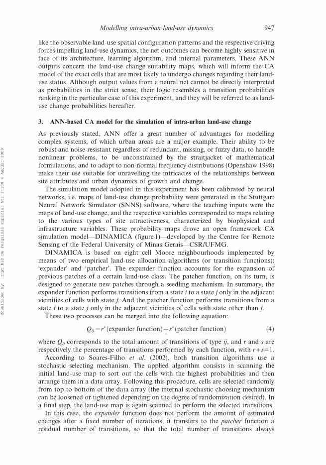
like the observable land-use spatial configuration patterns and the respective driving

forces impelling land-use dynamics, the net outcomes can become highly sensitive inface of its architecture, learning algorithm, and internal parameters. These ANN

outputs concern the land-use change suitability maps, which will inform the CA

model of the exact cells that are most likely to undergo changes regarding their land-

use status. Although output values from a neural net cannot be directly interpreted

as probabilities in the strict sense, their logic resembles a transition probabilities

ranking in the particular case of this experiment, and they will be referred to as land-

use change probabilities hereafter.

3. ANN-based CA model for the simulation of intra-urban land-use change

As previously stated, ANN offer a great number of advantages for modelling

complex systems, of which urban areas are a major example. Their ability to be

robust and noise-resistant regardless of redundant, missing, or fuzzy data, to handle

nonlinear problems, to be unconstrained by the straitjacket of mathematical

formulations, and to adapt to non-normal frequency distributions (Openshaw 1998)

make their use suitable for unravelling the intricacies of the relationships between

site attributes and urban dynamics of growth and change.

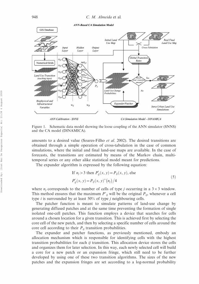
The simulation model adopted in this experiment has been calibrated by neural

networks, i.e. maps of land-use change probability were generated in the Stuttgart

Neural Network Simulator (SNNS) software, where the teaching inputs were the

maps of land-use change, and the respective variables corresponded to maps relatingto the various types of site attractiveness, characterized by biophysical and

infrastructure variables. These probability maps drove an open framework CA

simulation model—DINAMICA (figure 1)—developed by the Centre for Remote

Sensing of the Federal University of Minas Gerais—CSR/UFMG.

DINAMICA is based on eight cell Moore neighbourhoods implemented by

means of two empirical land-use allocation algorithms (or transition functions):

‘expander’ and ‘patcher’. The expander function accounts for the expansion of

previous patches of a certain land-use class. The patcher function, on its turn, is

designed to generate new patches through a seedling mechanism. In summary, the

expander function performs transitions from a state i to a state j only in the adjacent

vicinities of cells with state j. And the patcher function performs transitions from astate i to a state j only in the adjacent vicinities of cells with state other than j.

These two processes can be merged into the following equation:

Qij~r� expander functionð Þzs� patcher functionð Þ ð4Þ

where Qij corresponds to the total amount of transitions of type ij, and r and s are

respectively the percentage of transitions performed by each function, with r + s51.

According to Soares-Filho et al. (2002), both transition algorithms use a

stochastic selecting mechanism. The applied algorithm consists in scanning the

initial land-use map to sort out the cells with the highest probabilities and then

arrange them in a data array. Following this procedure, cells are selected randomly

from top to bottom of the data array (the internal stochastic choosing mechanismcan be loosened or tightened depending on the degree of randomization desired). In

a final step, the land-use map is again scanned to perform the selected transitions.

In this case, the expander function does not perform the amount of estimated

changes after a fixed number of iterations; it transfers to the patcher function a

residual number of transitions, so that the total number of transitions always



amounts to a desired value (Soares-Filho et al. 2002). The desired transitions are

obtained through a simple operation of cross-tabulation in the case of common

simulations, where the initial and final land-use maps are available. In the case of

forecasts, the transitions are estimated by means of the Markov chain, multi-

temporal series or any other alike statistical model meant for predictions.

The expander algorithm is expressed by the following equation:

If njw3 then P0ij x, yð Þ~Pij x, yð Þ, else

P0ij x, yð Þ~Pij x, yð Þ� nj

� ��4

ð5Þ

where nj corresponds to the number of cells of type j occurring in a 363 window.

This method ensures that the maximum P9ij will be the original Pij, whenever a cell

type i is surrounded by at least 50% of type j neighbouring cells.

The patcher function is meant to simulate patterns of land-use change by

generating diffused patches and at the same time preventing the formation of single

isolated one-cell patches. This function employs a device that searches for cells

around a chosen location for a given transition. This is achieved first by selecting the

core cell of the new patch, and then by selecting a specific number of cells around the

core cell according to their Pij transition probabilities.

The expander and patcher functions, as previously mentioned, embody an

allocation mechanism which is responsible for identifying cells with the highest

transition probabilities for each ij transition. This allocation device stores the cells

and organizes them for later selection. In this way, each newly selected cell will build

a core for a new patch or an expansion fringe, which still need to be further

developed by using one of these two transition algorithms. The sizes of the new

patches and the expansion fringes are set according to a log-normal probability

Figure 1. Schematic data model showing the loose coupling of the ANN simulator (SNNS)and the CA model (DINAMICA).



distribution, whose parameters are determined as a function of the mean size and

variance of each type of patch and expansion fringe to be generated (Soares-Filho

et al. 2002).

4. Applications

4.1 Study area and the GIS database

The ANN-based CA simulation model was applied to a medium-sized city,

Piracicaba, located in the Midwest of Sao Paulo State, at the margins of the

Piracicaba River, south-east of Brazil. The city comprised a total of 198 407

inhabitants in the initial time of simulation (1985), which rose to 309 531 inhabitants

in 1999. In this period, the annual population growth rate was around 1.56%, and

the resulting impact in the urban area was marked by the massive expansion of

existing residential areas together with a mushrooming of peripheral residential

settlements, which have been mostly incorporated into the main urban agglomera-

tion. Besides experiencing a rapid development concerning the residential use,

Piracicaba also witnessed intra-urban land-use changes like the increase in

industrial, institutional, and leisure areas (figure 2).

The city land-use maps in 1985 and 1999 were obtained from the Piracicaba

Municipal Secretariat for Town Planning. They were scanned, converted to vector

format in AutoCad, and then later pre-processed using SPRING GIS (developed by

the Images Processing Division of the Brazilian National Institute for Space

Research—DPI-INPE). These official maps do not always correspond to the real

situation, since they do not indicate informal (not legalized) settlements on the one

hand, and on the other hand, they show some of the legally approved settlements

that have not been built. To cope with these eventual disparities, satellite imagery

has been used to update the land-use maps exclusively regarding residential

settlements. Two Landsat images (WRS 220/76) were employed for this end: a TM-5

scene of 10 August 1985, and a second scene of 16 July 1999. The latest image was

georeferenced by means of an official topographic chart (UTM—SAD-69) with a

scale of 1:50 000, and the total average error was 1.2 pixels (with the tolerance

threshold lying around 1.5–2.0 pixels). It was then used for co-registering the 1985

image, and the total error amounted to only 0.3 pixel. The geographic coordinates of

the control points were later used for the registration of the city maps in vector

format using SPRING. Such maps were finally superimposed on linearly enhanced

colour composites of the registered images (4R_7G_1B), allowing a visual

crosscheck of existent and non-existent settlements.

For the purpose of simplifying the land-use maps, they were subject to

generalization procedures. Similar zones were reclassified to only one category,

e.g. residential zones of different densities were all reclassified to simply residential,

and special use and social infrastructure zones were reclassified to institutional.

Eight land-use zone categories were defined: residential, commercial, industrial,

services, institutional, leisure/recreation, water bodies, and non-urban use. Districts

located farther than 10 km from the main urban agglomeration were excluded from

the analysis, and the traffic network and minor non-occupied areas were disregarded

in the simulations.

All data used in this application were resampled to 50 m650 m for a better visual

adequacy of the maps (coarser resolutions would otherwise result in unpleasant

jags), but also with the aim of keeping a number of cells that would enable faster



simulations. The adopted resolution formed a grid containing 334 lines and 360

columns, with a total of 120 240 cells (30 060 ha) defining the region for simulation.

4.2 Exploratory analysis

One of the first steps in the exploratory analysis is the identification of the existing

types of intra-urban land-use change. A simple cross-tabulation (figure 3) between

the initial and final land-use maps provides this information (table 1), besides

quantifying the amount of change in terms of percentage, also called global

transition rates (table 2). These rates express the likelihood of change in the study

area as a whole, regardless of the influence of the driving (biophysical and

Figure 3. Land use change in Piracicaba from 1985 to 1999.

Figure 2. Generalized land-use maps in Piracicaba in 1985 (left) and 1999 (right).



infrastructure) variables. In some cases, they can be referred to as ‘global transition

probabilities’.

After identifying the existent land-use transitions, the next step concerns the

determination of the different sets of variables governing each of the four types of

change. The variables available for the modelling analysis do not always represent

the set of necessary variables able to produce ideal simulation results. In fact, intra-

urban land-use dynamics is subject to sudden and unforeseeable forces, like

landlords’ decisions to develop certain areas in disregard of others. In other words,

land-use transitions are more likely to be determined by some factors than others

depending on the processes of acquisition and development undertaken by

developers and consumers of land (Almeida et al. 2003). But in a general way,

there is indeed a set of decisive factors for urban land-use transitions, in the sense

that they substantially respond for the main drivers of such changes. And these

precise factors have effectively guided the modelling experiment at issue.

The several maps of biophysical and infrastructure variables have been generated

on the basis of the information extracted from land-use maps, like distances to

certain uses, distances to the Piracicaba River as well as distances to different

categories of the traffic network, such as paved and non-paved urban or interurban

roads. In all cases, the Euclidean distance has been used, and methods to initially

sort out the ideal set of variables to explain a given type of land-use change were

based on heuristic procedures. These procedures basically regard the visualization of

distinct maps of variables (distances in grey scale) superposed on maps of land-use

transition, so as to identify those that are more meaningful to explain the different

types of land-use change. A map of land-use transition was made for each respective

type of land-use change (NU_RES; NU_IND; NU_INST; NU_LEIS) through

reclassification of the cross-tabulation map. These maps of transition indicate with

different colours the areas of change and no change, and a black colour is assigned

to areas not associated with the land-use change under consideration, i.e. all areas

Table 1. Existent land-use transitions.

Notation Land-use transition

NU_RES Non-urban to residentialNU_IND Non-urban to industrialNU_INST Non-urban to institutionalNU_LEIS Non-urban to leisure/recreation

Table 2. Global transition rates for Piracicaba, 1985–1999.

Landuse NonU Res Comm Indust Inst Serv

Waterbodies Leis/rec

NonU 0.8353 0.1501 0 0.0113 0.0028 0 0 0.0005Res 0 1 0 0 0 0 0 0Comm 0 0 1 0 0 0 0 0Indust 0 0 0 1 0 0 0 0Inst 0 0 0 0 1 0 0 0Serv 0 0 0 0 0 1 0 0Water 0 0 0 0 0 0 1 0Leis/Rec

0 0 0 0 0 0 0 1



where the land-use at the initial time of simulation differs from the initial use of the

transition considered. All the overlays were carried out in spring, which enables

transparency in-between layers.

The natural environment (soil, vegetation, relief, conservation areas) has not been

regarded as a decisive driver for land-use change. In other words, natural

characteristics of the physical environment, excluding the Piracicaba River, have

not been considered as impedances to urban growth at a more generalized level. The

city sites are relatively flat, with mild slopes, and present no constraints regarding

soil, vegetation and conservation areas.

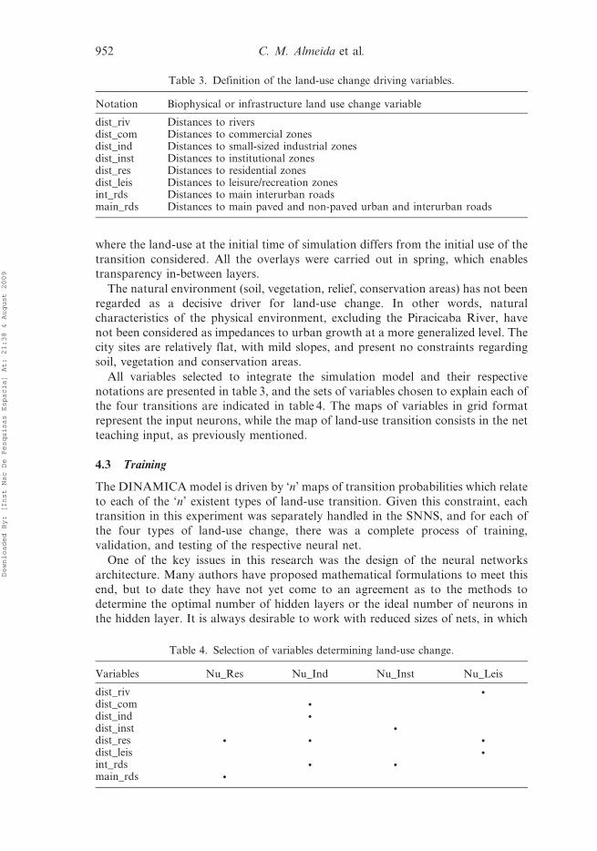
All variables selected to integrate the simulation model and their respective

notations are presented in table 3, and the sets of variables chosen to explain each of

the four transitions are indicated in table 4. The maps of variables in grid format

represent the input neurons, while the map of land-use transition consists in the net

teaching input, as previously mentioned.

4.3 Training

The DINAMICA model is driven by ‘n’ maps of transition probabilities which relate

to each of the ‘n’ existent types of land-use transition. Given this constraint, each

transition in this experiment was separately handled in the SNNS, and for each of

the four types of land-use change, there was a complete process of training,

validation, and testing of the respective neural net.

One of the key issues in this research was the design of the neural networks

architecture. Many authors have proposed mathematical formulations to meet this

end, but to date they have not yet come to an agreement as to the methods to

determine the optimal number of hidden layers or the ideal number of neurons in

the hidden layer. It is always desirable to work with reduced sizes of nets, in which

Table 3. Definition of the land-use change driving variables.

Notation Biophysical or infrastructure land use change variable

dist_riv Distances to riversdist_com Distances to commercial zonesdist_ind Distances to small-sized industrial zonesdist_inst Distances to institutional zonesdist_res Distances to residential zonesdist_leis Distances to leisure/recreation zonesint_rds Distances to main interurban roadsmain_rds Distances to main paved and non-paved urban and interurban roads

Table 4. Selection of variables determining land-use change.

Variables Nu_Res Nu_Ind Nu_Inst Nu_Leis

dist_riv Ndist_com Ndist_ind Ndist_inst Ndist_res N N Ndist_leis Nint_rds N Nmain_rds N



fast training and good performance can be ensured. For Kavzoglu and Mather

(1999), nets with more neurons or layers present the advantage to learn more

complex patterns, besides being less influenced by the initial random weights (Paola

and Schowengerdt 1997). But these complex neural nets, on the other hand, demand

more time for training and do not generalize well with unknown data, given the

excessive memorization of noise found in the training data sets (Haykin 1999).

According to Kolmogorov’s theorem, any continuous function W: XnRRc can be

implemented through a three-layer neural network with n neurons in the input layer,

(2n + 1) neurons in the single hidden layer, and c nodes in the output layer (Wang

1994). Fletcher and Goss (1993) suggested that the ideal number of neurons in the

hidden layer would be between 2n + 1 andffiffiffiffiffiffiffiffiffiffiffiffiffiffi2nzmp

, where n corresponds to the

number of neurons in the input layer, and m, to the number of neurons in the output

layer. Despite these divergences, there is a general consensus among researchers in

the field of urban CA modelling that empiricism is a reasonable way to determine

the best neural net structure for a specific problem (Li and Yeh 2001, Yeh and Li

2003, Guan and Wang 2005). All the four neural nets used in this experiment present

only one hidden layer with six neurons. The neurons in the input layer correspond to

the driving variables respectively available for each land-use change, and the output

layer presents just a single neuron, which refers to the local land-use transition

probabilities (table 5). The internal parameters of the nets were heuristically

determined.

The maps of land-use transition, used as teaching inputs, were converted into

grids, where 0.99 was assigned to the areas of change, 0.01, to the areas of no

change, and 0.000001 to the areas not concerned in the land-use change under

consideration. In the face of the sigmoid nature of the activation function, absolute

values of 0 and 1 were avoided in order to prevent excessively large values of weights

(Kavzoglu and Mather 2003) and, hence, biases in the numerical ranking of the

output nets. The grids generated in SPRING with extension SPR were converted

into ASCII format for their insertion in the neural network simulator (SNNS).

A special routine was created in C + + to randomly select 12 000 grid points,

which accounts for nearly 10% of the total amount of pixels in the study area, and to

further organize them in a array of 120 lines by 100 columns. Samples of this size

were used both as the training and validation sets, and the whole area was used as

the test set.

As already mentioned, the learning was interrupted when the validation set error

reached its minimum (figure 4). The SNNS displays three different types of error

Table 5. Parameters used in the neural nets.

Type oftransition

Trainingalgorithm

Inputneurons

Hiddenneurons

Numberof cycles

Initialupdate-value

(D0)

Maximumstep size(Dmax)

Weight-decay (a)

NU_RES ResilientBackProp

2 6 30 0.1 50 4

NU_IND ResilientBackProp

4 6 20 0.1 50 4

NU_INST ResilientBackProp

2 6 20 0.1 50 4

NU_LEIS ResilientBackProp

3 6 20 0.1 50 4



according to the number of cycles: the overall sum-of-the-squares of the output

error (SSE); the overall mean square error (MSE), which refers to the average of the

square of the error, namely the average of the difference between the desired

response or teaching input (ti) and the actual system output (oi); and the SSE divided

by the number of output units (SSE/out), which, for the kth training pattern, is:

SSE=out~1

no: of outputs

Xtk{okð Þ2 ð6Þ

The output grids were converted in thematic maps so as to allow a visual

comparison between such maps of local transition probabilities (output neurons)

and the respective maps of land-use transition, which correspond to the teaching

inputs (figure 5). This comparison enables a final empirical evaluation of the neural

nets performance. It is worth remarking that the DINAMICA model automatically

sets to 0 (zero) the areas where the land use at the initial time of simulation differs

from the initial use of the transition considered, in the cases when the maps of

transition probabilities are generated within the DINAMICA environment through

statistical methods. Since the maps of transition probabilities were produced by the

SNNS, areas with high transition probabilities were somehow overestimated. But

this surplus is disregarded when the DINAMICA algorithms entrusted with the

cells’ land-use change scan the maps of transition, for they take into account the

actual cells use according to the initial land-use map, and hence, the areas that can

effectively undergo changes are considerably reduced.

5. Validation

For assessing the accuracy of the CA simulation model performance, fuzzy

similarity measures applied within a neighbourhood context were used. Several

validation methods operating on a pixel vicinity basis have been proposed (Costanza

1989, Pontius 2002, Hagen 2003), aimed at depicting the spatial patterns similarity

between a simulated and reference map, so as to relax the strictness of the pixel-by-

pixel agreement. The fuzzy similarity method employed in this work is a variation of

Figure 4. Error decay curve for the training set (dark grey) and validation set (light grey)regarding the ‘NU_INST’ neural net.



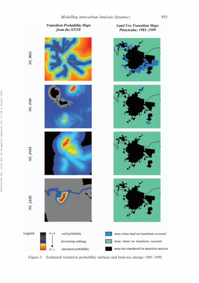
Figure 5. Estimated transition probability surfaces and land-use change: 1985–1999.



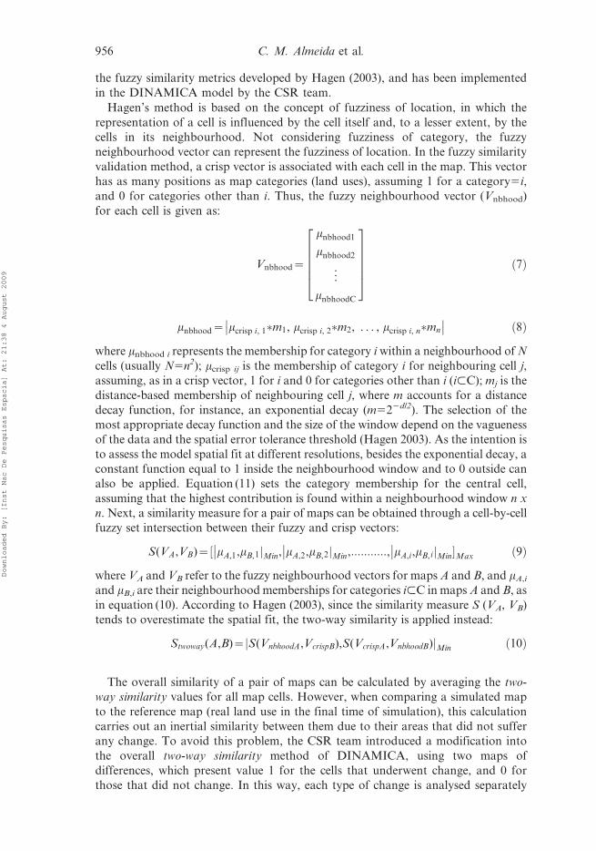
the fuzzy similarity metrics developed by Hagen (2003), and has been implemented

in the DINAMICA model by the CSR team.

Hagen’s method is based on the concept of fuzziness of location, in which the

representation of a cell is influenced by the cell itself and, to a lesser extent, by the

cells in its neighbourhood. Not considering fuzziness of category, the fuzzy

neighbourhood vector can represent the fuzziness of location. In the fuzzy similarity

validation method, a crisp vector is associated with each cell in the map. This vector

has as many positions as map categories (land uses), assuming 1 for a category5i,

and 0 for categories other than i. Thus, the fuzzy neighbourhood vector (Vnbhood)

for each cell is given as:

Vnbhood~

mnbhood1

mnbhood2

..

.

mnbhoodC

266664

377775

ð7Þ

mnbhood~ mcrisp i, 1�m1, mcrisp i, 2�m2, . . . , mcrisp i, n�mn

�� ð8Þ

where mnbhood i represents the membership for category i within a neighbourhood of N

cells (usually N5n2); mcrisp ij is the membership of category i for neighbouring cell j,

assuming, as in a crisp vector, 1 for i and 0 for categories other than i (i,C); mj is the

distance-based membership of neighbouring cell j, where m accounts for a distance

decay function, for instance, an exponential decay (m522d/2). The selection of the

most appropriate decay function and the size of the window depend on the vagueness

of the data and the spatial error tolerance threshold (Hagen 2003). As the intention is

to assess the model spatial fit at different resolutions, besides the exponential decay, a

constant function equal to 1 inside the neighbourhood window and to 0 outside can

also be applied. Equation (11) sets the category membership for the central cell,

assuming that the highest contribution is found within a neighbourhood window n x

n. Next, a similarity measure for a pair of maps can be obtained through a cell-by-cell

fuzzy set intersection between their fuzzy and crisp vectors:

S(VA,VB)~½ mA,1

�� ,mB,1jMin, mA,2

�� ,mB,2jMin,:::::::::::, mA,i

�� ,mB,ijMin�Max ð9Þ

where VA and VB refer to the fuzzy neighbourhood vectors for maps A and B, and mA,i

and mB,i are their neighbourhood memberships for categories i,C in maps A and B, as

in equation (10). According to Hagen (2003), since the similarity measure S (VA, VB)

tends to overestimate the spatial fit, the two-way similarity is applied instead:

Stwoway(A,B)~ Sj (VnbhoodA,VcrispB),S(VcrispA,VnbhoodB)jMin ð10Þ

The overall similarity of a pair of maps can be calculated by averaging the two-

way similarity values for all map cells. However, when comparing a simulated map

to the reference map (real land use in the final time of simulation), this calculation

carries out an inertial similarity between them due to their areas that did not suffer

any change. To avoid this problem, the CSR team introduced a modification into

the overall two-way similarity method of DINAMICA, using two maps of

differences, which present value 1 for the cells that underwent change, and 0 for

those that did not change. In this way, each type of change is analysed separately



using pairwise comparisons involving maps of differences: (i) between the initial

land-use map and a simulated one and (ii) between the same initial land-use map

and the reference one. This modification is able to tackle two matters. First, as it

deals with only one type of change at a time, the overall two-way similarity measure

can be applied to the entire map, regardless of the different number of cells per

category. Second, the inherited similitude between the initial and simulated maps

can be eliminated from this comparison by simply ignoring the null cells from the

overall count. However, there are two ways of performing this function. One

consists of counting only two-way similarity values for non-null cells in the first map

of difference, and the other consists in doing the opposite. As a result, three

measures of overall similarity are obtained, with the third representing the average

of the two ways of counting. As random pattern maps tend to score higher due to

chance depending on the manner in which the nulls are counted, it is advisable to

pay close attention to the minimum overall similarity value. This method has proven

to be the most comprehensive when compared with the aforementioned methods, as

it yields fitness measures with the highest contrast for a series of synthetic patterns

that depart from a perfect fit to a totally random pattern (Soares-Filho et al. 2004).

6. Simulations and discussion

Based on the assignment of appropriate weights to the input variables, the SNNS-

generated maps of local transition probabilities drove the CA simulation model—

DINAMICA. This model is also guided by internal parameters, determined

empirically, and which concern the average size and variance of patches and the

relative proportion of the transition algorithms (table 6). Due to the randomness of

the DINAMICA transition algorithms, even though the same internal parameters

are kept in different runs, different simulation results will be produced after each run

of the model. In this way, the three best urban land-use simulation results for the

city of Piracicaba in the period 1985–1999 are presented in figure 6.

It is observed that the transition from non-urban to residential use (NU_RES)

largely depends on the previous existence of residential settlements in their

surroundings, because this implies the possibility of extending existing nearby

infrastructure. It also depends on the available accessibility to such areas. The

implementation of large institutional areas (NU_INST) occurs near peripheral

roads and previously existent institutional areas, since they grow as extensions of

already established institutional zones. Likewise this transition, the expansion of

industrial districts (NU_IND) also requires the proximity to previously existent

industrial zones and the availability of road access. This can be explained by the fact

that in the industrial production process, the output of certain industries represents

Table 6. DINAMICA internal parameters for the simulation of urban land-use change inPiracicaba: 1985–1999.

Type oftransition

Average size ofpatches (ha)

Variance ofpatch size

(ha)Proportion of

‘expander’Proportion of

‘patcher’Number ofiterations

NU_RES 300 30 0.85 0.15 10NU_IND 150 1 0.45 0.55 10NU_INST 75 1 1.0 0 10NU_LEIS 20 0 1.0 0 10



the input of other ones, which raises the need of rationalization and optimization of

costs by the clustering of plants interrelated in the same production chain. This

transition supposes as well the nearness to the labour-force supply centres

(peripheral residential areas) and also a location not too far from commercial

zones, since industrial activities depend on the supply of commercial goods. New

leisure and recreation zones (NU_LEIS) also take place adjacent to already existent

zones of this type, since they are commonly created as extensions of the latter ones.

These areas are created along low and flat riverbanks, since they are floodable and

hence unsuitable for sheltering other urban uses. They are also strategically located

in relation to their catchment area, i.e. near central residential areas, which are those

sheltering higher population densities and which in fact correspond to the demand

market for leisure and recreation. It is implied by the above analyses that the land-

use transitions show compliance with economic theories of urban growth and

change, where there is a continuous search for the optimal location, able to ensure

Figure 6. Three best simulations compared with actual land use in 1999. The centralcommercial zone (orange) and the services corridors (dark yellow) did not undergo anytransitions during the observed time period. The new residential (dark blue) and institutionalareas (light yellow) as well as the leisure and recreational zones (red) were well modelled,particularly in the first and second simulations.



competitive real estate prices, good accessibility, rationalization of transportation

costs, and a strategic location in relation to supply and demand markets.

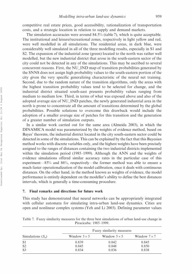
The simulation accuracies were around 84.5% (table 7), which is quite acceptable.

The institutional and leisure/recreational zones, respectively in light yellow and red,

were well modelled in all simulations. The residential areas, in dark blue, were

considerably well simulated in all of the three modelling results, especially in S1 and

S2. The expansion of the industrial zone (green) located to the north was rather well

modelled, but the new industrial district that arose in the south-eastern sector of the

city could not be detected in any of the simulations. This may be ascribed to several

concurrent reasons. First, the NU_IND map of transition probabilities generated by

the SNNS does not assign high probability values to the south-eastern portion of the

city given the very specific generalizing characteristic of the neural net training.

Second, due to the random nature of the transition algorithms, only the areas with

the highest transition probability values tend to be selected for change, and the

industrial district situated south-east presents probability values ranging from

medium to medium low. Third, in terms of what was exposed above and also of the

adopted average size of NU_IND patches, the newly generated industrial area in the

north is prone to concentrate all the amount of transitions determined by the global

probabilities. Possible solutions to overcome this drawback would include the

adoption of a smaller average size of patches for this transition and the generation

of a greater number of simulation outputs.

In a similar work carried out for the same area (Almeida 2003), in which the

DINAMICA model was parameterized by the weights of evidence method, based on

Bayes’ theorem, the industrial district located in the city south-eastern sector could be

detected in some of the simulations. This can be explained by the fact that this Bayesian

method works with discrete variables only, and the highest weights have been precisely

assigned to the ranges of distances containing the two industrial districts implemented

within the simulation period (1985–1999). Although the ANN and the weights of

evidence simulations offered similar accuracy rates in the particular case of this

experiment—85% and 86%, respectively—the former method was able to ensure a

much faster operationalization of the model calibration, once it deals with continuous

distances. On the other hand, in the method known as weights of evidence, the model

performance is entirely dependent on the modeller’s ability to define the best distances

intervals, which is generally a time-consuming procedure.

7. Final remarks and directions for future work

This study has demonstrated that neural networks can be appropriately integrated

with cellular automata for simulating intra-urban land-use dynamics. Cities are

open and nonlinear complex systems (Yeh and Li 2003). Defining parameter values

Table 7. Fuzzy similarity measures for the three best simulations of urban land-use change inPiracicaba: 1985–1999.

Simulations (Sn)

Fuzzy similarity measures

Window 363 Window 565 Window 767

S1 0.839 0.842 0.845S2 0.845 0.848 0.850S3 0.834 0.836 0.838



for assessing the relative importance of the intra-urban land-use change drivers in

traditional CA models is usually done on a basis of trial-and-error approaches,

which rely on the test of many possible parameter values in the search of an optimal

fit (Li and Yeh 2002). These procedures are commonly computation-intensive and

time-consuming, and do not always provide the best results. Neural networks, in

view of their ability to model nonlinear features and handle noisy, redundant, and

inaccurate spatial data, were shown to be robust and efficient for calibrating such

models, thus saving time and effort in automatically determining these parameter

values.

The ANN-based CA simulation model has been successfully applied to a medium-

sized town, Piracicaba, located in Sao Paulo State, south-east of Brazil.

DINAMICA is endowed with a stochastic structure, which embodies unpredict-

ability and chance in the logic of land-use change as observed in reality. And this is

precisely what differs DINAMICA from other exclusively ANN-based simulation

models (Yeh and Li 2003, Pijanowski et al. 2005), in which neural networks are used

not only for parameterizing the model, i.e. assessing the variables weights, but also

for accomplishing land-use transitions. In such models, randomization does not play

a direct role in the transitions themselves.

The ANN-generated maps of transition probabilities reflect the influence the set

of selected variables have in defining the compatibility extent between the predicted

and real land-use change areas, the latter shown in the land-use transition maps.

Researchers, planners, practitioners, and consultants in the urban field are able to

deal interactively with the model, so as to include or suppress one or more variables

and then evaluate the resulting impacts such changes produce in the land-use change

probabilities and land-use simulation maps. In this sense, the SNNS-generated maps

of transition probabilities can help planners and policy makers understand the

spatial driving forces and current trends of intra-urban dynamics, and hence

subsidise their actions towards urban development and regulations as well as

technical and social infrastructure implementation. Since knowledge can be easily

learned by the model and stored for further simulation (Li and Yeh 2001), future

land-use change alternatives could also be simulated on the basis of ANN-calibrated

land-use transition probability maps, so as to anticipate possible urban development

scenarios and orientate upcoming planning actions and policies.

Neural networks present though some inherent limitations in the sense that they

do not offer explicit knowledge on the process of assessing the weights of variables

driving land-use change. Moreover, the user’s intervention in defining the training

algorithm, the net architecture and its parameters are still important for the quality

of results. The SNNS environment itself enables users to initially assign more

importance to certain driving variables (input neurons) in comparison with others,

according to their a priori judgements. In this way, further studies are needed to

assess the responsiveness of simulations in the face of variations in the type,

structure, and internal parameters of the network.

Acknowledgements

The authors wish to thank the Piracicaba Water Supply and Waste Water Disposal

Department and the Piracicaba Planning Secretariat for providing the city maps. We

are also grateful for the help and cooperation of the technical and administrative

staff of the Centre for Remote Sensing of the Federal University of Minas Gerais

(CSR-UFMG). This study has received financial support from the Remote Sensing



Division of the Brazilian National Institute for Space Research (DSR/INPE). And

finally, the authors would like to thank the anonymous reviewers for their valuable

contributions in improving the quality of this paper.

ReferencesALMEIDA, C.M., 2003, Spatial dynamic modelling as a planning tool: simulation of urban

land use change in Bauru and Piracicaba (SP), Brazil. Sao Jose dos Campos.

Published PhD thesis, Brazilian National Institute for Space Research (INPE-10567-

TDI/942/B).

ALMEIDA, C.M., BATTY, M., MONTEIRO, A.V.M., CAMARA, G., SOARES-FILHO, B.S.,

CERQUEIRA, G.C. and PENNACHIN, C.L., 2003, Stochastic cellular automata

modelling of urban land use dynamics: empirical development and estimation.

Computers, Environment and Urban Systems, 27, pp. 481–509.

BATTY, M., COUCLELIS, H. and EICHEN, M., 1997, Urban systems as cellular automata.

Environmental and Planning B, 24, pp. 175–192.

BISHOP, C.M., 1995, Neural Networks for Pattern Recognition (Oxford: Oxford University

Press).

CLARKE, K.C. and GAYDOS, L., 1998, Loose-coupling a cellular automaton model and GIS:

long-term urban growth predictions for San Francisco and Baltimore. International

Journal of Geographical Information Science, 12, pp. 699–714.

CLARKE, K.C., HOPPEN, S. and GAYDOS, L.J., 1997, A self-modifying cellular automaton

model of historical urbanization in the San Francisco Bay area. Environment and

Planning B, 24, pp. 247–261.

COSTANZA, R., 1989, Model goodness of fit: a multiple resolution procedure. Ecological

Modeling, 47, pp. 199–215.

COUCLELIS, H., 1985, Cellular worlds: a framework for modeling micro-macro dynamics.

Environmental and Planning A, 17, pp. 585–596.

DEADMAN, P., BROWN, R.D. and GIMBLETT, P., 1993, Modeling rural residential settlement

patterns with cellular automata. Journal of Environmental Management, 37, pp.

147–160.

ENGELEN, G., WHITE, R. and ULJEE, I., 1997, Integrating constrained cellular automata

models, GIS and decision support tools for urban planning and policy making. In

Decision Support Systems in Urban Planning, H.P.J. Timmermans (Ed.), pp. 125–155

(London: E&FN Spon, 1997).

FISCHER, M.M. and ABRAHART, R.J., 2000, Neurocomputing—Tools for Geographers. In

GeoComputation, S. Openshaw and R.J. Abrahart (Eds), pp. 187–217 (New York:

Taylor & Francis, 2000).

FLETCHER, D. and GOSS, E., 1993, Forecasting with neural networks: an application using

bankruptcy data. Information and Management, 24, pp. 159–167.

GUAN, Q. and WANG, L., 2005, An Artificial-Neural-Network-Based Constrained CA

Model for Simulating Urban Growth and Its Application. In Auto-Carto Con-

ference, 18–23 March 2005, Las Vegas, NV. Available online at: http://www.

geog.ucsb.edu/,guan/papers/ Guan_AutoCarto2005.pdf (accessed 26 December

2005).

HAGEN, A., 2003, Multi-method assessment of map similarity. In 5th AGILE Conference on

Geographic Information Science, 25–27 April 2002, Palma, Spain (Palma: Universitat

de les Illes Balears), pp. 171–182.

HAYKIN, S.S., 1999, Neural Networks: A Comprehensive Foundation (Upper Saddle River, NJ:

Prentice-Hall).

KAVZOGLU, T. and MATHER, P.M., 1999, Pruning artificial neural networks: an example

using land cover classification of multi-sensor images. International Journal of Remote

Sensing, 20, pp. 2787–2803.



KAVZOGLU, T. and MATHER, P.M., 2003, The use of backpropagation artificial neural

networks in land cover classification. International Journal of Remote Sensing, 24, pp.

4907–4938.

LI, X. and YEH, A.G., 2000, Modeling sustainable urban development by the integration of

constrained cellular automata and GIS. International Journal of Geographical

Information Science, 14, pp. 131–152.

LI, X. and YEH, A.G., 2001, Calibration of cellular automata by using neural networks for the

simulation of complex urban systems. Environmental and Planning A, 33, pp.

1445–1462.

LI, X. and YEH, A.G., 2002, Neural-network-based cellular automata for simulating multiple

land use changes using GIS. International Journal of Geographical Information

Science, 16, pp. 323–343.

MOORE, T., 2000, Geospatial expert systems. In GeoComputation, S. Openshaw and R.J.

Abrahart (Eds), pp. 127–159 (New York: Taylor & Francis, 2000).

OPENSHAW, S., 1998, Neural network, genetic, and fuzzy logic models of spatial interaction.

Environmental and Planning A, 30, pp. 1857–1872.

PAOLA, J.D. and SCHOWENGERDT, R.A., 1997, The effect of neural-network structure on a

multispectral land-use/land-cover classification. Photogrammetric Engineering &

Remote Sensing, 63, pp. 535–544.

PHIPPS, M., 1989, Dynamical behaviour of cellular automata under constraints of

neighbourhood coherence. Geographical Analysis, 21, pp. 197–215.

PHIPPS, M. and LANGLOIS, A., 1997, Spatial dynamics, cellular automata, and parallel

processing computers. Environmental and Planning B, 24, pp. 193–204.

PIJANOWSKI, B.C., BROWN, D., SHELLITO, B. and MANIK, G., 2002a, Using neural networks

and GIS to forecast land use changes: A land transformation model. Computers,

Environment and Urban Systems, 26, pp. 553–575.

PIJANOWSKI, B.C., PITHADIA, S., SHELLITO, B.A. and ALEXANDRIDIS, K., 2005, Calibrating a

neural network-based urban change model for two metropolitan areas of the Upper

Midwest of the United States. International Journal of Geographical Information

Science, 19, pp. 197–215.

PIJANOWSKI, B.C., SHELLITO, B.A., PITHADIA, S. and ALEXANDRIDIS, K., 2002b, Using

artificial neural networks, geographic information systems and remote sensing to

model urban sprawl in coastal watersheds along eastern Lake Michigan. Lakes and

Reservoirs, 7, pp. 271–285.

PONTIUS, G., 2002, Statistical methods to partition effects of quantity and location during

comparison of categorical maps at multiple resolutions. Photogrammetric Engineering

and Remote Sensing, 68, pp. 1041–1049.

RIEDMILLER, M. and BRAUN, H., 1993, A direct adaptive method for faster backpropagation

learning: the RPROP algorithm. In IEEE International Conference on Neural

Networks, 28 March–1 April 1993, San Francisco (San Francisco: ICNN), pp.

586–591.

RUMELHART, D.E., HINTON, G.E. and WILLIAMS, R.J., 1986, Learning representations by

back-propagation errors. Nature, 323, pp. 533–536.

SOARES-FILHO, B.S., ALENCAR, A., NEPSTAD, D., CERQUEIRA, G.C., DIAL, M., DEL, C.,

SOLOZARNO, L. and VOLL, E., 2004, Simulating the response of land-cover changes to

road paving and governance along a major Amazon Highway: the Santarem-Cuiaba

corridor. Global Change Biology, 10, pp. 745–764.

SOARES-FILHO, B.S., CERQUEIRA, G.C. and PENNACHIN, C.L., 2002, DINAMICA—a

stochastic cellular automata model designed to simulate the landscape dynamics in

an Amazonian colonization frontier. Ecological Modelling, 154, pp. 217–235.

TAKEYAMA, M. and COUCLELIS, H., 1997, Map dynamics: integrating cellular automata and

GIS through geo-algebra. International Journal of Geographical Information Science,

11, pp. 73–91.



WANG, F., 1994, The use of artificial neural networks in a geographical information system

for agricultural land-suitability assessment. Environment and Planning A, 26, pp.

265–284.

WARD, D.P., MURRAY, A.T. and PHINN, S.R., 1999, An optimized cellular automata

approach for sustainable urban development in rapidly urbanizing regions. Available

online at: http://www.geovista.psu.edu/sites/geocomp99/Gc99/025/gc_025.htm

(accessed 30 October 2002).

WU, F., 1996, A linguistic cellular automata simulation approach for sustainable urban

development in a fast growing region. Computers, Environment and Urban Systems,

20, pp. 367–387.

YEH, A.G. and LI, X., 2003, Simulation of development alternatives using neural networks,

cellular automata, and GIS for urban planning. Photogrammetric Engineering and

Remote Sensing, 69, pp. 1043–1052.



Artigo IJGIS

Documents

Transcript of Artigo IJGIS