7 BAB 2 LANDASAN TEORI 2.1 Artificial Intelligence Artificial ...
Upload
khangminh22Category
view
2download
0
Artificial Financial Markets: AnAgent Based Approach to
Reproduce Stylized Facts and tostudy the Red Queen Effect
by
Serafin Martinez-Jaramillo
Submitted to the
Centre for Computational Finance and Economic Agents
for the degree of
Philosophiae Doctor
at the
UNIVERSITY OF ESSEX
June 2007
Signature of Author . . . . . . . . . . . . . . . . . . . . . . . . . . . . . . . . . . . . . . . . . . . . . . . . . . . . . . . . . . . . . . . . . . .
Centre for Computational Finance and Economic Agents
Supervisor: Professor Edward P. K. TsangTitle: Professor at the Computer Science Department of the University of Essex, DeputyDirector of CCFEA
Co-supervisor: Professor Sheri MarkoseTitle: Professor at the Economics Department of the University of Essex, Director ofCCFEA
Abstract
Stock markets are very important in modern societies and their behaviour have serious
implications in a wide spectrum of the world’s population. Investors, governing bodies
and the society as a whole could benefit from better understanding of the behaviour of
stock markets. The traditional approach to analyze such systems is the use of analytical
models. However, the complexity of financial markets represents a big challenge to the
analytical approach. Most analytical models make simplifying assumptions, such as
perfect rationality and homogeneous investors, which threaten the validity of analytical
results. This motivates the use of alternative methods. For those reasons, the study of
such markets is a fertile field to use the agent-based methodology.
In this work, we developed an artificial financial market and used it to study the
behaviour of stock markets. In this market, we model technical, fundamental and noise
traders. The technical traders are non-simple genetic programming based agents that
co-evolve (by means of their fitness function) by predicting investment opportunities in
the market using technical analysis as the main tool. Such traders are equipped with
an investment strategy that we consider to be realistic and we avoid any kind of strong
assumptions about the agents’ rationality, utility function or risk aversion.
Changes in some parameters and in the agents behaviour produce different properties
of the stock price series that we analyze. In this paper we investigate the different
conditions under which the statistical properties of an artificial stock market resemble
those of the real financial markets. Additionally, we modelled the pressure to beat the
market by a behavioural constraint imposed on the agents related to the Red Queen
principle in evolution. The Red Queen principle is a metaphor of a co-evolutionary arms
race between species. We investigate the effect of such constraint on the price dynamics
and the wealth distribution of the agents after several periods of trading in the different
simulation cases. We have demonstrated how evolutionary computation plays a key role
in studying stock markets.
i

To Biliana and Serafito
ii

Acknowledgements
First of all I am eternally grateful to Professor Tsang for his invaluable help, this work
could not be possible without him and his patience. I am also grateful to my co-supervisor
Professor Sheri Markose whose always sharp comments made this research richer. I am
sure that we will find time and space to continue working together.
Thanks to my dearest Biliana and beloved Serafito, they make my life better, happier,
full of rewards and more importantly, full of hope.
Thanks to my mother, brothers, nieces and nephews. All of them are an encourage-
ment to work harder all the time. I am particulary grateful to the Kabadjovi family for
their tremendous support, encouragement and care, without their help this could not be
possible. My eternal gratitude to Idulia Isabel and Hector, our loved Chilean friends and
people of goodwill and infinite generosity.
I would like to acknowledge the Mexican people that through the CONACYT allowed
this dream to come true. I would also like to acknowledge all the people from the Banco
de Mexico that helped me during this process, specially to Dr. Jose Gerardo Quijano
Leon for his support during the process.
Many thanks to Lynda, Julie, Marisa, Ramona and all the administrative staff from
CCFEA, Economics and the Computer Science Departments. I am also grateful with
the Computer Science technical support officers, without their help I could not do all the
necessary experiments. I want to thank the wonderful people at the University’s nursery
that looked after my son with the generous help from the University of Essex’s Student
Support Office.
Special thanks to my compadres Alma Lilia and Luis Humberto for helping me all the
time. I am really grateful with Kalina and Tonatiuh for kindly accepting to proof-read
the thesis. I am in debt with the good teachers and fellow students that during my whole
academic formation helped me to understand our complex world a little bit better. Last
but not least, my special gratitude to my colleagues from CCFEA, Computer Science
and Economics from the University of Essex. I am going to miss you all a lot.
iii
Related publications
• S. Markose, E. P. K. Tsang, and S. Martinez-Jaramillo. The red queen principle
and the emergence of efficient Financial markets: an agent based approach. In P.
J. Angeline, 50 Z. Michalewicz, M. Schoenauer, X. Yao, and A. Zalzala, editors, 8th
Workshop on Economics and Heterogeneous Interacting Agents (WEHIA), volume
2, pages 1253-1259, Kiel, Germany, 5 2003. Springer.
• E. P. Tsang and S. Martinez-Jaramillo. Computational Finance. In IEEE Compu-
tational Intelligence Society Newsletter, pages 3-8. 2004.
• Martinez-Jaramillo S., Tsang E. P. K. and Markose S. “Co-evolution of Genetic
Programming Based Agents in an Artificial Stock Market,” 12th International Con-
ference on Computing in Economics and Finance, Limassol, Cyprus, June 22-24,
2006.
• S. Martinez-Jaramillo and E. P. K. Tsang. An Heterogeneous, Endogenous and
Co-evolutionary GP-based Financial Market. Submitted to: IEEE Transactions
on Evolutionary Computation, Under review.
iv
Contents
Abstract i
Acknowledgements iii
Related publications iv
1 Introduction 1
1.1 Background . . . . . . . . . . . . . . . . . . . . . . . . . . . . . . . . . . 1
1.2 Motivations . . . . . . . . . . . . . . . . . . . . . . . . . . . . . . . . . . 2
1.3 Our research agenda . . . . . . . . . . . . . . . . . . . . . . . . . . . . . 3
1.4 Organization of the thesis . . . . . . . . . . . . . . . . . . . . . . . . . . 4
2 Literature Survey 6
2.1 Financial markets . . . . . . . . . . . . . . . . . . . . . . . . . . . . . . . 6
2.1.1 Market Efficiency . . . . . . . . . . . . . . . . . . . . . . . . . . . 7
2.1.2 Statistical properties of stock returns . . . . . . . . . . . . . . . . 8
2.2 Investment strategies in stock markets . . . . . . . . . . . . . . . . . . . 15
2.2.1 Fundamental strategies . . . . . . . . . . . . . . . . . . . . . . . . 15
2.2.2 Momentum trading . . . . . . . . . . . . . . . . . . . . . . . . . . 16
2.2.3 Contrarian strategies . . . . . . . . . . . . . . . . . . . . . . . . . 17
2.2.4 Trading strategies based on technical analysis . . . . . . . . . . . 17
2.3 Agent-Based Computational Economics . . . . . . . . . . . . . . . . . . . 18
v
2.4 Evolutionary computation in economics and finance . . . . . . . . . . . . 20
2.4.1 Multi-agent systems for economic and financial simulations . . . . 21
2.4.2 Game Theory and Computer Science . . . . . . . . . . . . . . . . 22
2.4.3 Portfolio optimization . . . . . . . . . . . . . . . . . . . . . . . . 23
2.4.4 Financial forecasting . . . . . . . . . . . . . . . . . . . . . . . . . 24
2.5 Artificial Intelligence in financial forecasting . . . . . . . . . . . . . . . . 24
2.5.1 Artificial Neural Networks . . . . . . . . . . . . . . . . . . . . . . 25
2.5.2 Genetic Algorithms . . . . . . . . . . . . . . . . . . . . . . . . . . 25
2.5.3 Learning Classifier Systems . . . . . . . . . . . . . . . . . . . . . 26
2.5.4 Genetic Programming . . . . . . . . . . . . . . . . . . . . . . . . 26
2.5.5 Other Artificial Intelligence techniques . . . . . . . . . . . . . . . 27
3 Artificial financial markets, state-of-the-art 29
3.1 Survey of artificial financial markets research . . . . . . . . . . . . . . . . 30
3.1.1 Agents’ Trading Strategies: From “zero intelligence” to Artificial
Intelligence . . . . . . . . . . . . . . . . . . . . . . . . . . . . . . 32
3.1.2 Market Mechanism . . . . . . . . . . . . . . . . . . . . . . . . . . 34
3.1.3 Assets . . . . . . . . . . . . . . . . . . . . . . . . . . . . . . . . . 35
3.1.4 Learning . . . . . . . . . . . . . . . . . . . . . . . . . . . . . . . . 36
3.1.5 Calibration and validation . . . . . . . . . . . . . . . . . . . . . . 39
3.1.6 Time . . . . . . . . . . . . . . . . . . . . . . . . . . . . . . . . . . 40
3.2 Limitations . . . . . . . . . . . . . . . . . . . . . . . . . . . . . . . . . . 41
4 CHASM: Co-evolutionary Heterogeneous Artificial Stock Market 43
4.1 Overview of the model . . . . . . . . . . . . . . . . . . . . . . . . . . . . 43
4.2 Market mechanism . . . . . . . . . . . . . . . . . . . . . . . . . . . . . . 44
4.3 Traders . . . . . . . . . . . . . . . . . . . . . . . . . . . . . . . . . . . . 47
4.3.1 Noise traders . . . . . . . . . . . . . . . . . . . . . . . . . . . . . 47
4.3.2 Value Traders . . . . . . . . . . . . . . . . . . . . . . . . . . . . . 47
vi

4.3.3 Technical traders . . . . . . . . . . . . . . . . . . . . . . . . . . . 48
4.4 Forecasting with EDDIE . . . . . . . . . . . . . . . . . . . . . . . . . . . 50
4.5 Learning . . . . . . . . . . . . . . . . . . . . . . . . . . . . . . . . . . . . 54
4.6 Important Characteristics of CHASM . . . . . . . . . . . . . . . . . . . . 56
4.6.1 Market and limit orders . . . . . . . . . . . . . . . . . . . . . . . 56
4.6.2 Fundamental trading . . . . . . . . . . . . . . . . . . . . . . . . . 57
4.6.3 Indicators . . . . . . . . . . . . . . . . . . . . . . . . . . . . . . . 58
4.6.4 Computational Capability . . . . . . . . . . . . . . . . . . . . . . 60
4.6.5 Desired return and time horizon . . . . . . . . . . . . . . . . . . . 60
4.6.6 Trading proportion . . . . . . . . . . . . . . . . . . . . . . . . . . 61
4.6.7 Fitness function . . . . . . . . . . . . . . . . . . . . . . . . . . . . 62
4.7 CHASM: The software . . . . . . . . . . . . . . . . . . . . . . . . . . . . 62
4.7.1 Design . . . . . . . . . . . . . . . . . . . . . . . . . . . . . . . . . 62
4.7.2 Flexibility and extensibility of the platform . . . . . . . . . . . . . 66
4.7.3 Implementation . . . . . . . . . . . . . . . . . . . . . . . . . . . . 66
4.7.4 Parameters . . . . . . . . . . . . . . . . . . . . . . . . . . . . . . 68
5 Minimal Conditions for Stylized Facts in CHASM 73
5.1 Parameters and features exploration . . . . . . . . . . . . . . . . . . . . . 74
5.2 The base case . . . . . . . . . . . . . . . . . . . . . . . . . . . . . . . . . 74
5.3 Dimension exploration . . . . . . . . . . . . . . . . . . . . . . . . . . . . 78
5.3.1 Limit Orders . . . . . . . . . . . . . . . . . . . . . . . . . . . . . 78
5.3.2 Fundamental trading . . . . . . . . . . . . . . . . . . . . . . . . . 82
5.3.3 Indicators . . . . . . . . . . . . . . . . . . . . . . . . . . . . . . . 85
5.3.4 Computational capability . . . . . . . . . . . . . . . . . . . . . . 88
5.3.5 Desired return and time horizon . . . . . . . . . . . . . . . . . . . 91
5.3.6 Trading proportion . . . . . . . . . . . . . . . . . . . . . . . . . . 95
5.4 Statistics . . . . . . . . . . . . . . . . . . . . . . . . . . . . . . . . . . . . 104
5.5 Concluding Summary . . . . . . . . . . . . . . . . . . . . . . . . . . . . . 107
vii
6 Co-evolution in CHASM 111
6.1 Social learning and herd behaviour . . . . . . . . . . . . . . . . . . . . . 114
6.1.1 Individual versus Social Learning . . . . . . . . . . . . . . . . . . 114
6.1.2 Herd behaviour . . . . . . . . . . . . . . . . . . . . . . . . . . . . 116
6.2 The Red Queen principle in evolution and economics . . . . . . . . . . . 117
6.2.1 The Red Queen in CHASM . . . . . . . . . . . . . . . . . . . . . 118
6.2.2 Experimental design . . . . . . . . . . . . . . . . . . . . . . . . . 119
6.3 Case studies and results . . . . . . . . . . . . . . . . . . . . . . . . . . . 120
6.4 Concluding summary . . . . . . . . . . . . . . . . . . . . . . . . . . . . . 140
7 Conclusions 146
7.1 Summary . . . . . . . . . . . . . . . . . . . . . . . . . . . . . . . . . . . 146
7.2 Experiments summary . . . . . . . . . . . . . . . . . . . . . . . . . . . . 149
7.2.1 Initial training . . . . . . . . . . . . . . . . . . . . . . . . . . . . 149
7.2.2 Learning and wealth . . . . . . . . . . . . . . . . . . . . . . . . . 150
7.2.3 Fitness measure . . . . . . . . . . . . . . . . . . . . . . . . . . . . 150
7.2.4 Heterogeneity . . . . . . . . . . . . . . . . . . . . . . . . . . . . . 151
7.2.5 Learning and returns . . . . . . . . . . . . . . . . . . . . . . . . . 151
7.2.6 The Red Queen Principle . . . . . . . . . . . . . . . . . . . . . . 152
7.3 Contributions . . . . . . . . . . . . . . . . . . . . . . . . . . . . . . . . . 152
7.3.1 CHASM . . . . . . . . . . . . . . . . . . . . . . . . . . . . . . . . 153
7.3.2 Agents . . . . . . . . . . . . . . . . . . . . . . . . . . . . . . . . . 154
7.3.3 Learning in CHASM . . . . . . . . . . . . . . . . . . . . . . . . . 155
7.3.4 CHASM and Stylized Facts . . . . . . . . . . . . . . . . . . . . . 156
7.3.5 The Red Queen principle . . . . . . . . . . . . . . . . . . . . . . . 156
7.3.6 The role of heterogeneity . . . . . . . . . . . . . . . . . . . . . . . 157
7.4 Future research . . . . . . . . . . . . . . . . . . . . . . . . . . . . . . . . 158
viii

List of Figures
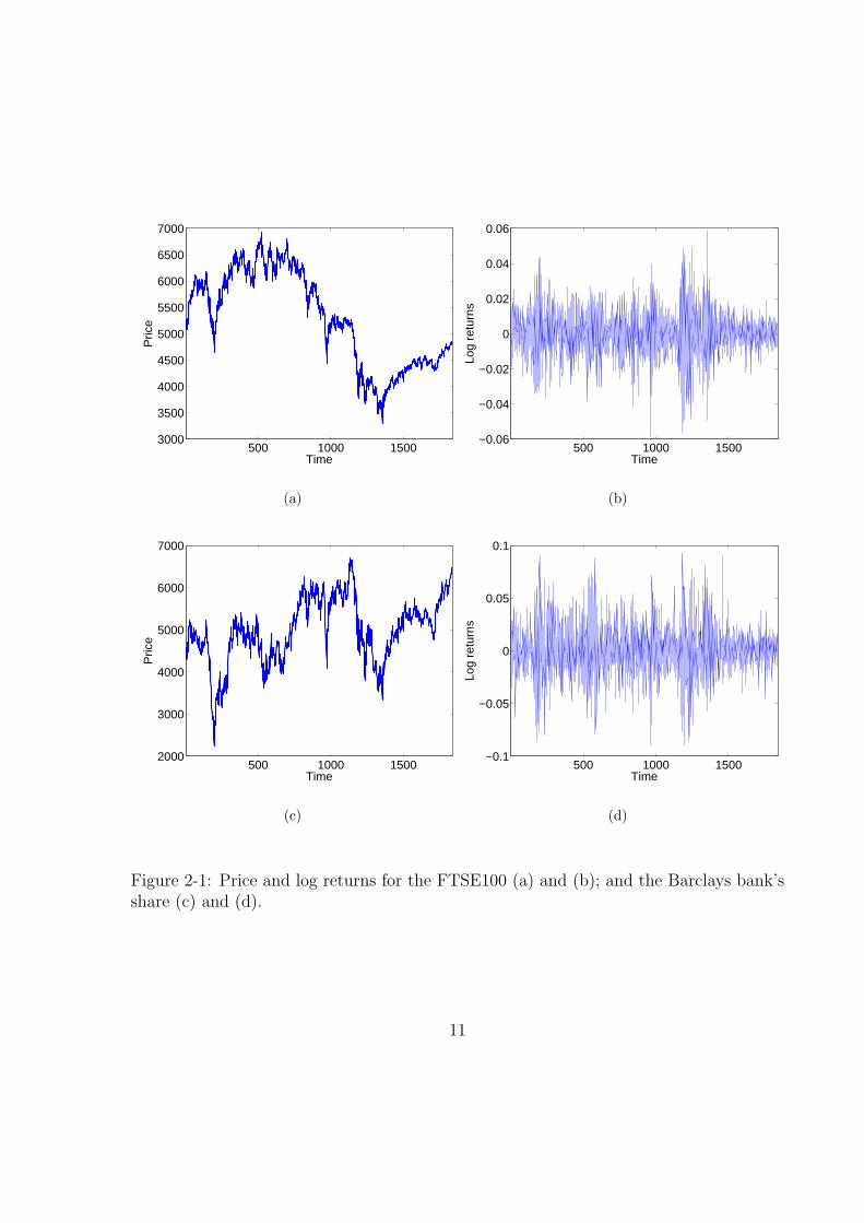
2-1 Price and log returns for the FTSE100 (a) and (b); and the Barclays bank’s
share (c) and (d). . . . . . . . . . . . . . . . . . . . . . . . . . . . . . . . 11
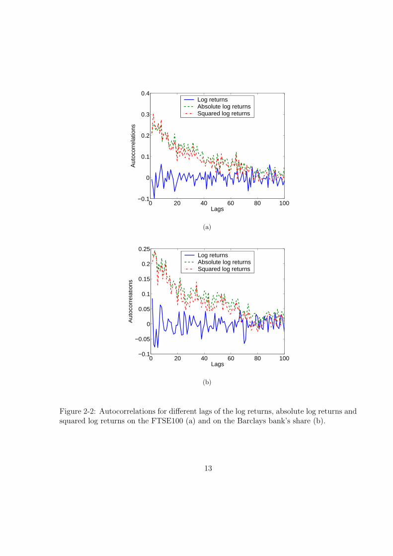
2-2 Autocorrelations for different lags of the log returns, absolute log returns
and squared log returns on the FTSE100 (a) and on the Barclays bank’s
share (b). . . . . . . . . . . . . . . . . . . . . . . . . . . . . . . . . . . . 13
4-1 Example of a decision tree. . . . . . . . . . . . . . . . . . . . . . . . . . . 51
4-2 Example of a decision rule interpreted from a decision tree . . . . . . . . 52
4-3 Examples of wealth evolution with (red dashed line) and without learning
(blue continuous line). . . . . . . . . . . . . . . . . . . . . . . . . . . . . 55
4-4 CHASM’s main screen. . . . . . . . . . . . . . . . . . . . . . . . . . . . . 63
4-5 CHASM java classes. . . . . . . . . . . . . . . . . . . . . . . . . . . . . . 64
4-6 Technical Trader java class. . . . . . . . . . . . . . . . . . . . . . . . . . 65
4-7 Parameters’ windows. . . . . . . . . . . . . . . . . . . . . . . . . . . . . . 69
4-8 Technical traders parameters’ window. . . . . . . . . . . . . . . . . . . . 72
5-1 Artificial Stock Market Parameter Study . . . . . . . . . . . . . . . . . . 75
5-2 Price and log returns for the Base Case. . . . . . . . . . . . . . . . . . . 77
5-3 Autocorrelations for different lags of the log returns, absolute log returns
and squared log returns on the Base Case. . . . . . . . . . . . . . . . . . 77
5-4 Base Case wealth distribution . . . . . . . . . . . . . . . . . . . . . . . . 78
5-5 Price and log returns for the Base Case without limit orders. . . . . . . . 80
ix
5-6 Autocorrelations for different lags of the log returns, absolute log returns
and squared log returns on the Base Case without limit orders being gen-
erated. . . . . . . . . . . . . . . . . . . . . . . . . . . . . . . . . . . . . . 81
5-7 Base Case without limit orders wealth distribution . . . . . . . . . . . . . 81
5-8 Price and log returns for the Base Case without fundamental trading. . . 83
5-9 Autocorrelations for different lags of the log returns, absolute log returns
and squared log returns on the Base Case without fundamental behaviour 84
5-10 Base Case without fundamental trading wealth distribution . . . . . . . . 85
5-11 Price and log returns for the Base Case with homogeneous indicators set
for all groups. . . . . . . . . . . . . . . . . . . . . . . . . . . . . . . . . . 86
5-12 Autocorrelations for different lags of the log returns, absolute log returns
and squared log returns on the Base Case with homogeneous information
for all groups. . . . . . . . . . . . . . . . . . . . . . . . . . . . . . . . . . 87
5-13 Base Case with homogeneous indicators set for all groups wealth distribution 88
5-14 Price and log returns for the Base Case with heterogeneous computational
capability for each group. . . . . . . . . . . . . . . . . . . . . . . . . . . . 90
5-15 Autocorrelations for different lags of the log returns, absolute log returns
and squared log returns on the Base Case with heterogeneous computa-
tional capability. . . . . . . . . . . . . . . . . . . . . . . . . . . . . . . . 90
5-16 Base Case with heterogeneous computational capability for each group
wealth distribution. . . . . . . . . . . . . . . . . . . . . . . . . . . . . . . 91
5-17 Price and log returns for the Base Case with heterogeneous desired return
and time horizon for each group. . . . . . . . . . . . . . . . . . . . . . . . 93
5-18 Autocorrelations for different lags of the log returns, absolute log returns
and squared log returns on the Base Case with heterogeneous desired rate
of return and time horizon. . . . . . . . . . . . . . . . . . . . . . . . . . . 93
5-19 Base Case with heterogeneous desired return and time horizon for each
group wealth distribution . . . . . . . . . . . . . . . . . . . . . . . . . . . 94
x
5-20 Price and log returns for the Base Case with values of 20%, 30% and 40%
for the trading proportion. . . . . . . . . . . . . . . . . . . . . . . . . . . 96
5-21 Price and log returns for the Base Case with values of 50%, 60% and 70%
for the trading proportion. . . . . . . . . . . . . . . . . . . . . . . . . . . 97
5-22 Price and log returns for the Base Case with values of 80%, 90% and 100%
for the trading proportion. . . . . . . . . . . . . . . . . . . . . . . . . . . 98
5-23 Autocorrelations for different lags of the log returns, absolute log returns
and squared log returns on the Base Case with trading proportion of 30%,
90% and 100%. . . . . . . . . . . . . . . . . . . . . . . . . . . . . . . . . 100
5-24 Base Case with a trading proportion of 20%, 30% and 40% wealth distri-
bution . . . . . . . . . . . . . . . . . . . . . . . . . . . . . . . . . . . . . 101
5-25 Base Case with a trading proportion of 50%, 60% and 70% wealth distri-
bution . . . . . . . . . . . . . . . . . . . . . . . . . . . . . . . . . . . . . 102
5-26 Base Case with a trading proportion of 80%, 90% and 100% wealth dis-
tribution . . . . . . . . . . . . . . . . . . . . . . . . . . . . . . . . . . . . 103
6-1 Case 1 prices and log returns . . . . . . . . . . . . . . . . . . . . . . . . . 124
6-2 Case 1 wealth distribution . . . . . . . . . . . . . . . . . . . . . . . . . . 125
6-3 Autocorrelations for different lags of the log returns, absolute log returns
and squared log returns on Case 1 with no learning taking place, learning
with fixed periodicity and learning under the Red Queen constraint. . . . 126
6-4 Case 2 prices and log returns . . . . . . . . . . . . . . . . . . . . . . . . . 129
6-5 Case 2 wealth distribution . . . . . . . . . . . . . . . . . . . . . . . . . . 130
6-6 Autocorrelations for different lags of the log returns, absolute log returns
and squared log returns on Case 2 with no learning taking place, learning
with fixed periodicity and learning under the Red Queen constraint. . . . 131
6-7 Case 3 prices and log returns . . . . . . . . . . . . . . . . . . . . . . . . . 134
6-8 Case 3 wealth distribution . . . . . . . . . . . . . . . . . . . . . . . . . . 135
xi

6-9 Autocorrelations for different lags of the log returns, absolute log returns
and squared log returns on Case 3 with no learning taking place, learning
with fixed periodicity and learning under the Red Queen constraint. . . . 137
6-10 Case 4 prices and log returns . . . . . . . . . . . . . . . . . . . . . . . . . 139
6-11 Case 4 wealth distribution . . . . . . . . . . . . . . . . . . . . . . . . . . 141
6-12 Autocorrelations for different lags of the log returns, absolute log returns
and squared log returns on Case 4 with no learning taking place, learning
with fixed periodicity and learning under the Red Queen constraint. . . . 142
xii

List of Tables
2.1 Statistics for the log returns FTSE100 and Barclays. . . . . . . . . . . . 14
4.1 A contingency table for three-class classification/prediction problem . . . 53
4.2 Indicators used by the agents to create investment rules . . . . . . . . . . 58
5.1 Statistics for the log returns Base Case I. . . . . . . . . . . . . . . . . . . 105
5.2 Statistics for the log returns Base Case II . . . . . . . . . . . . . . . . . . 106
5.3 Statistics for the log returns Base Case Trading Proportion I. . . . . . . . 106
5.4 Statistics for the log returns Base Case Trading Proportion II. . . . . . . 107
5.5 Evaluation criteria on stock prices for each group of experiments. . . . . 110
6.1 Statistics for the log returns Case 1 . . . . . . . . . . . . . . . . . . . . . 127
6.2 Statistics for the log returns Case 2 . . . . . . . . . . . . . . . . . . . . . 132
6.3 Statistics for the log returns Case 3 . . . . . . . . . . . . . . . . . . . . . 136
6.4 Statistics for the log returns Case 4 . . . . . . . . . . . . . . . . . . . . . 143
6.5 Evaluation criteria on stock prices for each group of experiments. . . . . 145
xiii
Chapter 1
Introduction
1.1 Background
The complexity of financial markets, represents a big challenge to the specialist in the
area. The traditional way of coping with the analysis of such markets is the use of ana-
lytical models. However, the analytical models present some difficulties and this has led
to the development of alternative methods for the analysis of such markets. The emerg-
ing fields of Agent-based Computational Economics (ACE) [189] and Computational
Finance [198], provide some means to tackle some of the limitations of the analytical
models in economics and finance. The ACE approach has been successfully applied in
several economic studies, varying from macroeconomic models to fish and payment cards
markets [8], [11], [111], [112], [2]. The study of financial markets, in particular, caught
the attention of an increasing number of researchers in this area.
Agent-based financial markets of different characteristics have been developed for the
study of such markets in the last decade since the influential Santa Fe Artificial Market
[16], [124]. Some of them differ from the original Santa Fe market on the type of agents
used like [53], [91], [149], [184], [208]; on market mechanism like [25], [91], [184], [208].
Other markets borrow ideas from statistical mechanics like [129], [130], [138]. Some
important research has been done modelling stock markets inspired on the Minority
1
Game like [42], [45]. There are financial simulated markets in which several stocks are
traded like in [56]. However, there are some criticisms to this approach like the problem of
calibration, the numerous parameters needed for the simulation program, the complexity
of the simulation, etc.
1.2 Motivations
“Levy, Solomon and Levy’s Microscopic Simulation of Financial Markets points us to-
wards the future of financial economics. If we restrict ourselves to models which can be
solved analytically, we will be modeling for our mutual entertainment, not to maximize
explanatory or predictive power.”
Harry M. Markowitz, President, Harry Markowitz Co., and Nobel Laureate in Eco-
nomics
The previous quote about the book [128] by one of the most influential authors in
financial economics can be considered as an inspiration for us in the development of our
work. We certainly pretend to increase the explanatory power of the financial models by
using novel but powerful techniques to overcome the limitations of the analytical models.
The contradictions between the existing theory and the empirical properties of the
stock market returns are the main driving force for some researchers to develop and use
different approaches to study financial markets. An additional aspect on the study of
financial markets is the complexity of the analytical models of such markets. Previous
to the development of some new simulation techniques, very important simplifying (un-
realistic) assumptions had to be made in order to allow tractability of the theoretical
models.
Artificial intelligence and in particular evolutionary computation have been used in
the past to study some financial and economic problems. However, the development of
a well established community of what is now known as the Agent Based Computational
Economics community facilitates the study of phenomena in financial markets that was
2

not possible in the past. Within such community, a vast number of works and a different
number of approaches are being produced by numbers in order to solve or gain more
understanding of some economic problems.
The influential work [16] and previously the development of the concept of bounded
rationality [177], [178], [179], [12] and [14], changed the way in which we conceive the
economic agents. This change in conception, changed dramatically the possibilities to
study some economic phenomena and in particular the Financial Markets. The new
models of economic agents have changed, there is no need any more of fully rational
representative agents, there is no need of homogeneous expectations and information
symmetry. Furthermore, the development of Artificially Adapted Agents [102] gives to
the economics science a way forward into the study of economic systems.
1.3 Our research agenda
Our approach to the modelling of artificial stock markets is different to the above men-
tioned cases mainly on the strategic behaviour of the agents. We use a very simple
market mechanism and non-simple agents, because our aim is to study the co-evolution
of the group of genetic programming based agents and the consequences on the price of
changes in the agents’ strategic behaviour. We believe that the modelling of the learning
behaviour of the agents is a central part of our research agenda. Regarding the agents’
learning process, we consider of extreme importance what Lucas wrote in [136]:
In general terms, we view or model an individual as a collection of decision
rules (rules that dictate the action to be taken in given situations) and a set
of preferences used to evaluate the outcomes arising from particular situation-
action combinations. These decision rules are continuously under review and
revision; new decision rules are tried and tested against experience, and rules
that produce desirable outcomes supplant those that do not.
3

There are many useful techniques to implement what Lucas’ defined as adaptive
learning, like genetic algorithms, as has been done in [40]. However, for the modelling of
the learning process described above by Lucas we will use genetic programming. Such
technique has been previously described as a suitable way to model economic learning in
[36]. The learning process that we used to model our agents’ behaviour will be described
with detail in Chapter 3.
Additionally, we are interested in finding the conditions under which the statistical
behaviour of the endogenously generated price resembles the behaviour of real prices.
Such task has been recognized as a very important one. Due to the complexity of the
simulated financial markets, it is difficult to know which features of the model is the
responsible for the appearance of such statistical properties. The market reported in this
work is composed by different types of traders: technical traders, fundamental traders,
and noise traders. The market mechanism, the agents’ strategic behaviour and the rele-
vant parameters will be described in detail in later chapters.
1.4 Organization of the thesis
This thesis is organized in the following way: In the second chapter we will introduce
four broad areas that are involved in our research: Financial Markets, Agent-Based Eco-
nomics, Evolutionary Computation in Economics and Finance and Artificial Intelligence
in Financial Forecasting. In such chapter, we provide references to some of the most
important works on each topic. However, it is not our intention to provide an exhaustive
review of the literature on each subject as that would take a lot of space and effort to be
done in a complete way.
In Chapter three we review the literature on Artificial Stock Markets, in particular
what we consider to be the state-of-the-art in this area. In this chapter we review some
of the most important works that have been done in the past and we review some of the
most recent works which we think could lead to promising areas of research in the future.
4

Chapter four deals with the description of the model and the computational platform
(CHASM) that we constructed in order to perform the experiments that we had in mind.
In such chapter we describe first the important characteristics of the model that are
going to be explored in order to obtain stylized facts. The computational platform is
later briefly described in software engineering terms and the more important parameters
are enumerated. Additionally, in Chapter four we report the results of an experiment on
learning in CHASM.
In Chapter five we describe the conditions under which some of the so called “stylized
facts” emerge in CHASM. The important characteristics in CHASM, previously described
in Chapter four, are explored and the experimental results are shown. In this chapter
we conclude with the features of the model that lead to the reproduction of some of the
universally exhibited statistical properties of the financial returns.
Chapter six deals with co-evolution in CHASM, the Red Queen principle and the
experimental results under what we called the Red Queen constraint. In this chapter,
experiments are performed in which the agents adapt to the environment (the market)
in two different ways. The first form of adaptation consists in that the agents change
their behaviour in fixed periods. The second form of adaptation is called the Red Queen
constraint and is inspired by the character of Lewis Caroll’s book Through the Looking
Glass.
Chapter seven concludes and summarizes the research findings of this work. The most
prominent findings are enumerated and the main contributions of our work to the ACE
field are described as well. Additionally, we describe some promising areas of research
along the line of our artificial stock market.
5
Chapter 2
Literature Survey
2.1 Financial markets
Financial markets can be broadly defined as a group of institutions that have the main
purpose of facilitating the exchange of assets. The asset that is going to be traded
obviously depends on the specific type of market. Some examples of such markets are:
stock markets, bond markets, money markets, commodity markets, foreign exchange
markets and derivatives markets.
Financial markets are a very important part of our everyday lives even if we do not
follow them closely. For example, everybody suffers the consequences of a stock market
crash, like the international market crash in 1987. Moreover, this phenomena (market
crashes) occurs with an unpleasant higher frequency than is predicted by the standard
economic theory.
One of the most important research issues in financial markets is the explanation of the
process that determines the asset prices and as a result the rate of return. There are many
models that can be used to explain such process, like the Capital Asset Pricing Model
(CAPM), the Arbitrage Pricing Theory (APT) or the Black-Scholes Option Pricing.
However, it is not our intention to give in this chapter an overview of such models, but
any introductory book to financial markets could help in this issue, like [172].
6

We are more interested in the sort of assumptions made in some of those models.
Some of such assumptions are believed to be false or at least unrealistic, like the assump-
tions of full rationality, information symmetry, homogeneous expectations, etc. However,
there are some phenomena that question the validity of the assumptions made by such
models, like the appearance of patterns on the prices. Furthermore, some empirical
studies contradict the predictions of such analytical models.
Another important concept in the study of financial markets is the concept of market
equilibrium. In such state, it is assumed that the price of the asset is adjusted so that the
demand to hold the asset equals its total stock. In a more general sense, the concept of
equilibrium can be considered one of the most important concepts in economic sciences.
However, in our ever changing real world it is difficult to imagine such static equilibrium
happening. In [15], Arthur explores deeply the implications of an economic world in
which things are not in equilibrium and he names his approach as out-of-equilibrium
economics.
2.1.1 Market Efficiency
“I’d be a bum in the street with a tin cup if the markets were efficient.”
Warren Buffett
The concept of market efficiency ([71] and [72]) has ruled the research agenda in Fi-
nancial Economics in the previous decades. It is considered one of the most important
concepts in finance and for some years has been at the centre of a debate. There exist
different forms of efficiency. However, we are interested just in what is known as informa-
tional efficiency. Markets are said to be informationally efficient if the price fully reflects
the available information [71].
One must be careful to interpret such definition of efficiency, the last part of the
phrase refers to the “available information”. This implies that the definition of market
efficiency depends on the information set. Furthermore, we can now derive an alternative
definition of market efficiency:
7
A market is efficient with respect to a particular information set φ if it is impossible
to make abnormal profits by using this set of information to formulate buying and selling
decisions. It is helpful to link the type of efficiency with the information set in the
following definitions of different market efficiencies:
• Weak Form Efficiency. In this case, the relevant information set comprises all
current and past prices.
• Semi-Strong Form Efficiency asserts that the asset market is efficient relative to all
publicly available information.
• Strong Form Efficiency asserts that the market for an asset is efficient relative to
all information including private information.
Market efficiency has been associated in the past with the concept of “random walk”
[142]. However, it is now a well known fact that the price changes do not follow a
random walk [134]. Moreover, it is commonly accepted that there are certain variables
that posses some predictability power on the price changes [74]. Beyond the debate of
market efficiency or the joint hypothesis test our work pretends to shed some light on the
way in which such efficiency is achieved or at least to explain the origins of the behaviour
of financial prices.
2.1.2 Statistical properties of stock returns
After the publication of the seminal review article in Market Efficiency [71], the arrival
of new econometric techniques has changed permanently the perception we had about
market efficiency. It seems that the empirical evidence of the behaviour of the financial
data points into a different direction than the market efficiency tells us. Alternatively,
it could be argued that the analytical models do not fully explain some of the statistical
behaviour of the financial prices.
8
The statistical analysis of the price time series is usually performed on the contin-
uously compounded return or log return. The log returns are defined in the following
way:
rt ≡ logPt
Pt−1
= pt − pt−1 (2.1)
where pt ≡ log Pt. Some of the advantages of such returns are first that the continu-
ously compound multiperiod return is the sum of continuously compounded single period
returns, and second that it is more easy to derive the time-series properties of additive
processes than multiplicative processes.
Time series of stock returns exhibit interesting statistical features which seem to be
common to a wide range of markets and time-periods. Such statistical properties are
known as “stylized facts” and have been reported for several types of financial data and
their presence seems to be ubiquitous in all sorts of financial markets [59], [138], [139].
Such statistical properties of the returns have become a very important benchmark
for the researchers of artificial financial markets. Such properties are the first step to
accomplish when building a simulated financial market [123]. The difficulty of replicating
such properties even with stochastic models is well expressed by Cont in [59]: “these
stylized facts are so constraining that it is not easy to exhibit even an (ad hoc) stochastic
process which possesses the same set of properties and one has to go to great lengths
to reproduce them with a model”. Moreover, some artificial markets try to explain the
origins of some of such stylized facts [137].
We will not report all of such stylized facts for our experiments due to different reasons,
like the frequency of our generated prices (which we will interpret as daily closing prices).
Therefore, we will describe briefly, as they are described by Cont in [59], the facts that
we will be reporting in later chapters:
1. Lack of autocorrelations: (linear) autocorrelations of returns are usually insignifi-
cant. However, this is not true for small intra-day time scales.
9

2. Volatility clustering: different measures of volatility display a positive autocorre-
lation over several days, which quantifies the fact that high-volatility events tend
to cluster in time. As noted by Mandelbrot, “large changes tend to be followed
by large changes, of either sign, and small changes tend to be followed by small
changes”.
3. Slow decay of autocorrelation in absolute returns: the autocorrelation function of
absolute returns decays slowly as a function of the time lag, roughly as a power
law with an exponent β ∈ [0.2, 0.4]. This is sometimes interpreted as a sign of
long-range dependence.
4. Heavy tails: The distribution of daily and higher frequency returns displays a heavy
tail with positive excess kurtosis. The tail index is finite, higher than two and less
than five for most assets, exchange rates and indexes.
5. Conditional heavy tails: even after correcting returns for volatility clustering (e.g.
via GARCH-type models), the residual time series still exhibit heavy tails. How-
ever, the tails are less heavy than in the unconditional distribution of returns.
6. Non Gaussianity: the stock returns on a weekly, daily and higher frequencies fail
to be normally distributed.
Figure 2-1, illustrates the daily closing prices 2-1(a) and log returns 2-1(b) for the
FTSE100 index and for the Barclays bank’s share 2-1(c) and 2-1(d) from the 2nd of
January 1998 to the 31st of December 2004.
In order to verify that our endogenously generated price mimics some of the above
described statistical properties, we will perform different sorts of test. For the first
described property, we will report the autocorrelations of the log returns, the absolute
log returns and the squared log returns for different time lags. The autocorrelation of
the absolute and squared log returns will allow us to investigate the phenomena known
as volatility clustering. Empirical studies in various stock indexes and stock prices have
10
500 1000 15003000
3500
4000
4500
5000
5500
6000
6500
7000
Time
Pric
e
(a)
500 1000 1500−0.06
−0.04
−0.02
0
0.02
0.04
0.06
TimeLo
g re
turn
s
(b)
500 1000 15002000
3000
4000
5000
6000
7000
Time
Pric
e
(c)
500 1000 1500−0.1
−0.05
0
0.05
0.1
Time
Log
retu
rns
(d)
Figure 2-1: Price and log returns for the FTSE100 (a) and (b); and the Barclays bank’sshare (c) and (d).
11
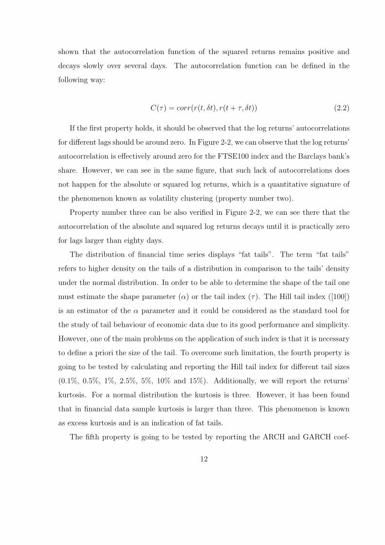
shown that the autocorrelation function of the squared returns remains positive and
decays slowly over several days. The autocorrelation function can be defined in the
following way:
C(τ) = corr(r(t, δt), r(t + τ, δt)) (2.2)
If the first property holds, it should be observed that the log returns’ autocorrelations
for different lags should be around zero. In Figure 2-2, we can observe that the log returns’
autocorrelation is effectively around zero for the FTSE100 index and the Barclays bank’s
share. However, we can see in the same figure, that such lack of autocorrelations does
not happen for the absolute or squared log returns, which is a quantitative signature of
the phenomenon known as volatility clustering (property number two).
Property number three can be also verified in Figure 2-2, we can see there that the
autocorrelation of the absolute and squared log returns decays until it is practically zero
for lags larger than eighty days.
The distribution of financial time series displays “fat tails”. The term “fat tails”
refers to higher density on the tails of a distribution in comparison to the tails’ density
under the normal distribution. In order to be able to determine the shape of the tail one
must estimate the shape parameter (α) or the tail index (τ). The Hill tail index ([100])
is an estimator of the α parameter and it could be considered as the standard tool for
the study of tail behaviour of economic data due to its good performance and simplicity.
However, one of the main problems on the application of such index is that it is necessary
to define a priori the size of the tail. To overcome such limitation, the fourth property is
going to be tested by calculating and reporting the Hill tail index for different tail sizes
(0.1%, 0.5%, 1%, 2.5%, 5%, 10% and 15%). Additionally, we will report the returns’
kurtosis. For a normal distribution the kurtosis is three. However, it has been found
that in financial data sample kurtosis is larger than three. This phenomenon is known
as excess kurtosis and is an indication of fat tails.
The fifth property is going to be tested by reporting the ARCH and GARCH coef-
12
0 20 40 60 80 100−0.1
0
0.1
0.2
0.3
0.4
Lags
Aut
ocor
rela
tions
Log returnsAbsolute log returnsSquared log returns
(a)
0 20 40 60 80 100−0.1
−0.05
0
0.05
0.1
0.15
0.2
0.25
Lags
Aut
ocor
rela
tions
Log returnsAbsolute log returnsSquared log returns
(b)
Figure 2-2: Autocorrelations for different lags of the log returns, absolute log returns andsquared log returns on the FTSE100 (a) and on the Barclays bank’s share (b).
13
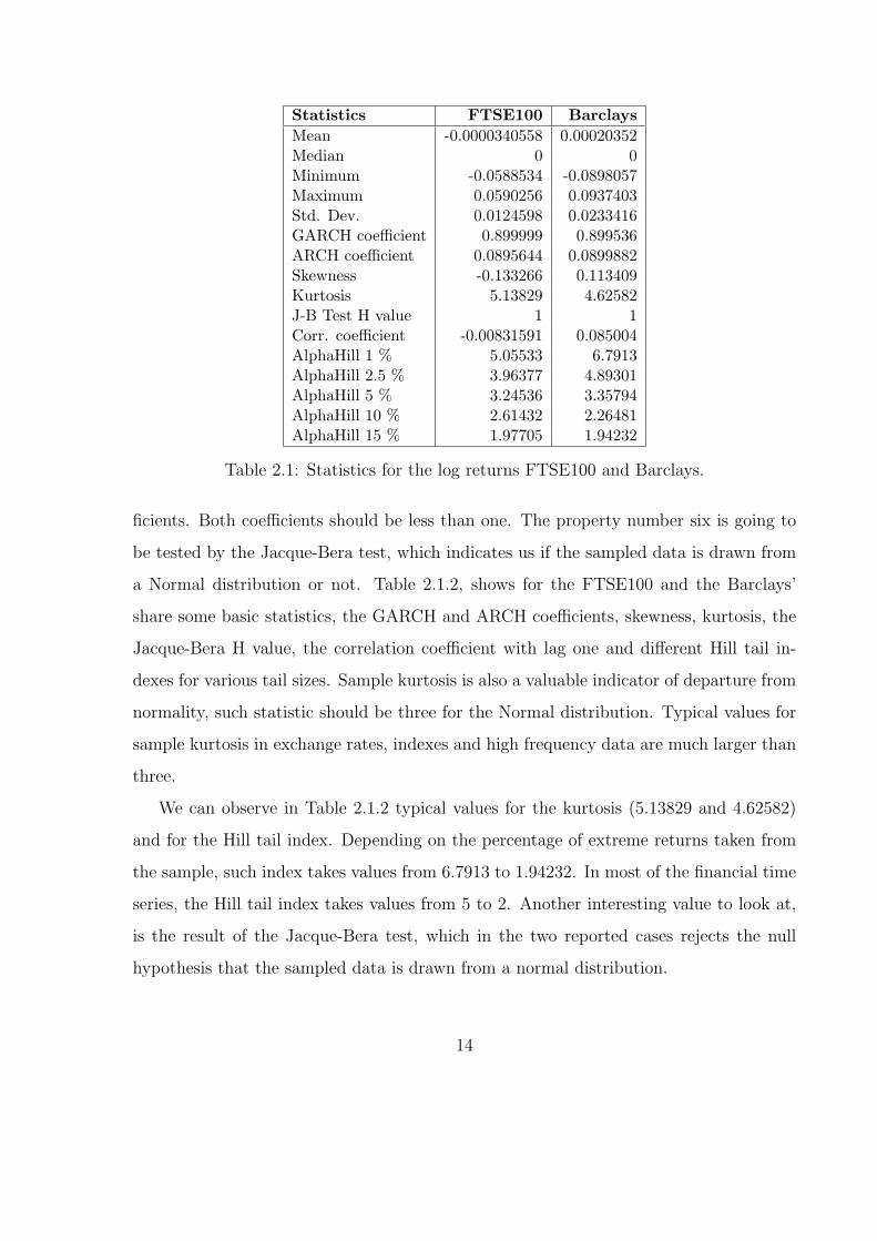
Statistics FTSE100 BarclaysMean -0.0000340558 0.00020352Median 0 0Minimum -0.0588534 -0.0898057Maximum 0.0590256 0.0937403Std. Dev. 0.0124598 0.0233416GARCH coefficient 0.899999 0.899536ARCH coefficient 0.0895644 0.0899882Skewness -0.133266 0.113409Kurtosis 5.13829 4.62582J-B Test H value 1 1Corr. coefficient -0.00831591 0.085004AlphaHill 1 % 5.05533 6.7913AlphaHill 2.5 % 3.96377 4.89301AlphaHill 5 % 3.24536 3.35794AlphaHill 10 % 2.61432 2.26481AlphaHill 15 % 1.97705 1.94232
Table 2.1: Statistics for the log returns FTSE100 and Barclays.
ficients. Both coefficients should be less than one. The property number six is going to
be tested by the Jacque-Bera test, which indicates us if the sampled data is drawn from
a Normal distribution or not. Table 2.1.2, shows for the FTSE100 and the Barclays’
share some basic statistics, the GARCH and ARCH coefficients, skewness, kurtosis, the
Jacque-Bera H value, the correlation coefficient with lag one and different Hill tail in-
dexes for various tail sizes. Sample kurtosis is also a valuable indicator of departure from
normality, such statistic should be three for the Normal distribution. Typical values for
sample kurtosis in exchange rates, indexes and high frequency data are much larger than
three.
We can observe in Table 2.1.2 typical values for the kurtosis (5.13829 and 4.62582)
and for the Hill tail index. Depending on the percentage of extreme returns taken from
the sample, such index takes values from 6.7913 to 1.94232. In most of the financial time
series, the Hill tail index takes values from 5 to 2. Another interesting value to look at,
is the result of the Jacque-Bera test, which in the two reported cases rejects the null
hypothesis that the sampled data is drawn from a normal distribution.
14
2.2 Investment strategies in stock markets
Financial time series are probably the most intensively studied of all. The reason for
this is obvious and is mostly related to the economic reward associated with a successful
forecasting of such time series. There are different ways in which an investor can define a
strategy. It is not our intention to give a full and detailed review of investment strategies,
we just want to exemplify the way in which an investment strategy can be defined.
In this section we will briefly describe some simple, yet commonly used trading strate-
gies. The reason to describe such strategies is because one of the most important decision
in the building of an artificial financial market is the strategic decision making of the in-
dividual agents. Therefore, if we want to endow our agents with a realistic investment
strategy we should know the sort of strategies that are currently being used by the real
investors.
It is not our intention to give a complete overview of all the different trading strategies
being used in the stock markets. A full review of such dimensions is far beyond the scope
of this thesis. Nevertheless, there is a plenty of information about such strategies in
books and the internet. The only recommendation is to be careful with the sources and
advices that are currently available on such books and sites.
2.2.1 Fundamental strategies
Fundamental analysis of stock prices is based on the analysis of the factors that could
affect such prices. These factors include information like financial reports, information
about the management of the company, earnings per share, revenue, cash flow, book-to-
market equity, earnings-to-price, earnings announcements, analyst upgrades and down-
grades, etc. Some researchers have found evidence of the relation between some of the
above information and the future returns [73], [115] and [74].
The basic idea in fundamental analysis is to produce what is known as the “funda-
mental value” by using all the previously mentioned factors. Once such fundamental
15
value has been obtained, the investor is able to compare such value with the current
security’s price and then she can take a position depending on the comparison. If the
price of a security is above the fundamental value, it is said to be “overvalued” and a
selling position or short selling position is recommended. If on the other hand, the price
of the security is below the fundamental value it is said to be “undervalued” and a buying
position is recommended.
A very important assumption on the technical analysis is that the security’s price is
always going to return to its fundamental value. Otherwise, the recommendations that
we explained before are meaningless. Therefore, the performance of such trading strategy
heavily depends on the accuracy of the perception of the fundamental value and on the
assumption that the price is always returning to its fundamental value.
2.2.2 Momentum trading
Momentum trading is said to take place when an investor buys past winners and sells past
losers. Despite of the simplicity of such strategies, it is believed that they are frequently
used by some mutual funds [156], [93], [94]. In [94], Grinblatt et al by using a measure
of momentum investment found that around 77 percent of mutual funds bought past
winners and sold past losers. Furthermore, momentum strategies could be responsible
for the abnormal profits earned by some mutual funds [156], [93], [94].
The volume has been recognized to provide useful information about a security’s price
change in the past [34]. In [125], Lee and Swaminathan find relationships between the
high and low trading volume and momentum and value strategies. In such work, the
authors provide plausible explanations for the intermediate horizon momentum and the
long horizon return reversal.
Momentum trading (and as a consequence contrarian trading) is related to two well
recognized regularities: overreaction and underreaction [27]. Underreaction consists that
on intermediate horizons, securities prices incorporate slowly the information. This means
that good or bad news have predictive power on the future returns. Overreaction happens
16
in longer horizons when the prices overreact to patterns of news pointing out on the same
direction. This means that securities that have had a long history of good or bad news
tend to become overpriced or underpriced. However, in the long term such valuations
will return to the mean [27].
2.2.3 Contrarian strategies
Contrarian strategies are very simple in principle like the momentum trading strategies.
Whenever an investor is using such strategies he is trying to capitalize on the overreaction
and underreaction of stock prices. Such overreaction and underreaction refer to the
finding that past winners would perform bad and that past losers could perform well in
the future. The probable reason for the above described phenomena is that investors
can be over exited by the past performance of an asset and believe that such trend will
continue. The opposite happens with the past losers: the investors probably think that
such asset is going to continue under-performing in the future.
There exist several theories of the reason why such type of strategies perform well. In
[73] Fama and French suggest that such good performance is due to the higher risk that is
being taken by the investors. On the other hand, in [115] Lakonishok et al. argue that the
good performance of such strategies is because they bet against investors that are over
optimistic of the performance of past winners and over pessimistic of the performance
of past losers. Furthermore, they find no evidence that such strategies bear more risk.
However, in [135] Lo and MacKinlay arrive to the conclusion that overreaction is not the
only source of contrarian investment profits.
2.2.4 Trading strategies based on technical analysis
Technical analysis has been on the trading arena for quite some time and it is believed
that is widely used in different markets [109], [157], [186]. Additionally, technical analysis
is by far the most common type of trading strategy in some markets like the foreign
exchange markets [158], [157].
17
Despite the long history of technical analysis and its widespread use, such technique
has been strongly criticized by some sectors of the academia and the industry. In [142],
Malkiel shares his opinion about technical analysis: “under scientific scrutiny, chart-
reading must share a pedestal with alchemy.” Nevertheless, there are numerous works
that suggest that technical analysis could be a profitable trading strategy [5], [34], [38],
[212], [61], [63], [64], [62], [103], [158], [159].
Technical analysis tries to identify patterns in the past prices and use them to predict
future movements and make an investment decision on that basis. Such technique is
mainly visual (although things have changed a lot recently) while one of its main com-
petitors, quantitative finance, is mainly numerical. The first person to use a technical
trading rule was Charles Dow, the editor of the Wall Street Journal, more than a hundred
years ago.
There are some recent modifications to the old techniques comming from different
areas like physics. In [17], Ausloos and Ivanova use the volume as the “physical mass” of
stocks and derive something that they call the generalized momentum indicator. In [103],
Hsu and Kuan reexamined the profitability of some trading rules taking into account the
well known problem of data snooping.
2.3 Agent-Based Computational Economics
Agent-based computational economics can be thought of as a branch of a wider area:
Agent-based Modelling. The field of Agent-based modelling is not restricted to economics,
it has been applied in social sciences in general [21], in some classical and not so classical
problems in computer science and in some other disciplines. In [22] Axelrod provides an
account of his experience using the Agent-based methodology for several problems and
he suggests that the Agent-based modelling can be seen as a bridge between disciplines.
Axelrod and Tesfatsion provide a good guide to the relevant literature of the Agent-based
modelling in [23]. In [50] there is a good introduction to agents in economics and finance;
18
in such work, Chen conceives the agents not just as economic agents but as computational
intelligent units.
Most of the economic and finance theory is based on what is known as investor
homogeneity or the representative agent. Agent-based Computational Economics (ACE)
is an emerging field of research in which the researchers can depart from the assumptions
of homogeneous expectations and perfect rationality by means of computational-based
economic agents. In [188], [187], [189] and [190], Tesfatsion surveys some of the most
important works and topics on this area of research.
In ACE one of the main goals is to explain the macro dynamics of the economy by
means of the micro interactions of the economic agents. This approach to the study of the
economy has been called a “bottom-up” approach in opposition to the more traditional
approaches in economics.
There are many different disciplines involved in this area, from which, computer
science can be distinguished as one of the most important ones. Another important
discipline that is somehow related to Agent-based computational economics is “Econo-
physics”. In [78], [144] and [140] there is an overview of the sort of economic research
done by physicists, the convergence in some areas with economists and the contributions
already made by some researchers in this field. Despite the interesting research being
done in econophysics, there is a certain reluctance from economists and physicists to fully
accept this new discipline.
There are some interesting works in which the Agent-based methodology is compared
with experiments performed with human beings [46] and [66]. In both works, the benefits
that each type of research has on each other are identified. Experimental research can
be used as an important method to calibrate an agent-based model. On the other hand,
agent-based simulations can be used to explain certain phenomena present in human
experiments. To summarize, there are many beneficial ways in which both types of
research influence each other.
According to Tesfatsion, the economic research being done with the ACE methodology
19
can pursue one of two main objectives: the first one is the constructive explanation of
macro phenomena and the second is the design of new economic mechanisms [187], [188]
and [189]. In [190] Tesfatsion updates the classification of the research being made
in ACE into four main categories: empirical understanding, normative understanding,
methodological advancement and finally qualitative insight and theory generation.
2.4 Evolutionary computation in economics and fi-
nance
Evolutionary computation possesses now a long tradition as a research tool in economics
and particulary in finance. The areas of research in economics and finance in which an
evolutionary technique is being used, are among the most relevant ones in both fields.
It is not exaggerated to say that evolutionary computation is at the heart of economics
and finance, sharing the place with more traditional tools. Some examples of the use of
evolutionary computation in economics can be [8], [39], [9], [180], [51], [52]. In finance,
evolutionary computation has a long lasting tradition, for example [29], [5].
Chen provides a good collection of papers that use either genetic algorithms or genetic
programming in finance [48]. In [198] there is a good introduction to the Computational
Finance field. In such paper the research agenda on the field is defined and some impor-
tant works are described. There are yet another two important works: on computational
intelligence [49] and on computationally intelligent agents [50] in economics and finance.
Despite the existence of several useful artificial intelligence techniques like neural
networks, a great body of research in computational economics and computational finance
employs some form of evolutionary computation. In the following subsections, some
examples of such applications will be provided and some of the most relevant works
are going to be briefly described. It would take a full survey paper to give a complete
account of all the work that has been done in economics and finance using evolutionary
computation. Nevertheless, our objective is just to show the relevance of evolutionary
20

computation in both fields and to introduce briefly the subject.
2.4.1 Multi-agent systems for economic and financial simula-
tions
One obvious place where is possible to find evolutionary computation techniques is in
the Multi-agent systems [80], [207], [182]. Genetic algorithms have been used for the
modelling of the agents’ learning in multi-agent simulations. In multi-agent simulations
of economics systems it is possible to find very different approaches and topics, just to
illustrate some few examples of the immense amount of works, lets take a look to the
following list:
• Electricity markets [6] (Learning Classifier System), [204] (This work is based onreinforcement learning).
• Payment card markets [1], [2] (Population Based Incremental Learning).
• Large value payments systems [209] (This work is based on reinforcement learning).
• Retail petrol markets [99] (Genetic Algorithms).
• Stock markets [16] (Learning Classifier System).
• Foreign exchange markets [10], [106] (Genetic Algorithms).
A fairly good introduction to the relevance of computational agents in economics and
finance can be found in [50].
Artificial financial markets
Financial markets are probably the markets that attract the most attention from very
different disciplines. This might be caused by the dynamism of such markets and the
importance that they have in our lives (for example the impact of financial crashes
in everyone’s economy). Another important aspects of financial markets is the highly
frequent information that they generate and that can be used to study them.
21
With all these elements present it is hard to imagine that the computer scientist could
not be fascinated by financial markets and in particular such markets have caught the
attention of researchers in Artificial Intelligence and multi-agent systems.
Since Genetic Algorithms have been used to perform financial forecasting in the past
[29], it was natural to combine them within the framework of a multi-agent system to
model the induction performed by an autonomous agent participating in a simulated
financial market [102], [16].
Different sorts of evolutionary techniques have been used to model economic agents
participating in an artificially simulated financial market. Among such techniques we
can mention: genetic algorithms, learning classifier systems, population-based incremen-
tal learning and genetic programming. There are, however, other artificial intelligence
techniques used in the modelling of economic agents in financial markets like Artificial
Neural Networks.
We will give a more detailed account of the research in Artificial Financial Markets
in the next chapter.
2.4.2 Game Theory and Computer Science
Game theory is one of the best established theories in economics and it has been used
to model the interactions between the economic agents extensively. One of the main
assumptions in game theory is that the agents behave in a rational way. However, in real
life human behaviour is frequently irrational.
Computer science has been used in traditional game theory problems, like the strategic
behaviour of agents in auctions, auction mechanism design, etc. This approach can be
useful where analytical solutions have not been found by providing approximate solutions
in such complex problems.
The iterative prisoners’ dilemma is one of the most studied games by researchers
from computer science [20]. The prisoners’ dilemma is a classic game that consists of the
decision making process by two prisoners which can choose to cooperate or to defect. In
22
the case that the two prisoners choose to cooperate they get a payoff of three each, in
the case that both choose to defect they get a payoff of one each and in the case that
any of them decides to defect and the other to cooperate, the former gets a payoff of five
and the later a payoff of zero. In equilibrium, both players decide to defect despite the
fact that would be better for them to cooperate.
Axelrod organized a tournament on the iterated prisoners’ dilemma in which he asked
people from game theory and amateurs to provide him with strategies. The surprising
result was that a very simple strategy (Tit for Tat) won the tournament [20]. After
the reporting of the results from such tournament, Axelrod was able to provide some
mathematical results on how cooperation can emerge in a population of egoists. The
previous example clearly illustrates how beneficial was the use of computer science to
obtain theoretical results in a problem where analytical methods alone have not delivered
the desired results.
2.4.3 Portfolio optimization
Portfolio optimization is probably the most important task in finance. Almost everything
in finance surrounds this problem: the determination of the price, the estimation of the
volatility, the correlation among stocks. The portfolio selection problem can be described
in a simple way as the problem of choosing the assets and the proportion of such assets
in an investor’s portfolio that wants to maximize his profits and minimize the risk.
The literature on portfolio optimization is vast and it is not our intention to provide
a full review of this area here. However, we will try to provide some interesting examples
of research being done with an extensive use of computation.
The population of papers on portfolio optimization using any form of evolutionary
computation is very big. Nevertheless, we can say that [155], [191], [183], [97], [181],
[146], [65] and [145] are some interesting works on portfolio optimization that use some
form of evolutionary computation or artificial intelligence.
23
2.4.4 Financial forecasting
Some of the most relevant evolutionary techniques that have been used in the past to
perform financial forecasting are: genetic algorithms, learning classifier systems and ge-
netic programming. In the next section, a brief description of the different works on each
of the above mentioned techniques is provided.
2.5 Artificial Intelligence in financial forecasting
Despite the wide acceptance of the Efficient Market Hypothesis among academics and the
implications of such theory for the predictability of price changes, financial forecasting
has always been one of the most intense research fields, due to the implications of a
successful technique to foresee the changes in financial time series. The possible reward
of a useful tool to discover the changes in the prices or the returns of financial assets, is
the single and most important motivation to invest an enormous amount of effort and
money in this field. Furthermore, the availability of financial data (both in quantity and
in quality) causes that a great number of resources are dedicated to the single task of
predicting future price changes.
Financial time series are probably the most studied time series by numerous disci-
plines and Computer Science could not be the exception. Moreover, there is a growing
acceptance among practitioners of the techniques and tools based or inspired by some
important areas of research in Computer Science.
Artificial Intelligence in general and Evolutionary Computation in particular are two
of the most influential areas involved in the design of techniques and tools to perform
some forms of financial forecasting. Among the most successful ones we can find Artificial
Neural Networks, Genetic Algorithms, Genetic Programming and Learning Classifier
Systems.
24
2.5.1 Artificial Neural Networks
Artificial Neural Networks (ANN’s) are probably the most exploited artificial intelligence
technique in financial forecasting, their use is wide across banks and even countries. The
literature on the topic is huge, we will just cite some classic works and books: [193], [166],
[24], [213]. Additionally, this technique has been applied on different fields of finance and
in [206] it is possible to find a good survey of the literature between 1990 and 1996.
Another more recent survey can be found in [171].
Artificial neural networks have achieved something that some other artificial intelli-
gence techniques would like to have: acceptance among the practitioners and academics
in finance. However, such technique has often been seen as a “black box” in contrast to
techniques like GAs or GP. Nevertheless, such view has been recently challenged in [31].
The input data is a crucial factor on the success or failure of ANN’s in financial
forecasting as it is in all the other techniques. However, this aspect becomes critical in
ANN’s due to the lack of flexibility of such technique, although some interesting research
has been done in which ANN’s are combined with GAs [98]. Some other relevant examples
of this area of research are: [96], [210], [63], [28].
2.5.2 Genetic Algorithms
Genetic Algorithms (GAs) were invented by John H. Holland [101]. A good introductory
book to the topic is [154]. Such algorithms have been very popular in optimization and
machine learning problems. As we will see later, financial forecasting is not the only task
that GAs successfully perform in Computational Economics and Finance. Moreover,
such technique has been used as an important part of the modelling of economic learning
in the context of agent-based computational economics and in the context of multi-agent
systems in general.
In the past, GAs have been used in several important works to perform financial
forecasting like in [29], [143], [5] and [126]. However, they have not been used frequently
in recent works mainly due to some of the limitations of GAs like the fixed size structure
25
of the individuals and their representation.
Despite the fact that GAs are not used intensively nowadays to perform financial
forecasting, they can be used as a meta-heuristic or in conjunction with other techniques
to improve the predictions’ performance like in [201] and [98].
2.5.3 Learning Classifier Systems
A learning classifier system is basically a machine learning mechanism in which a popu-
lation of rules is selected and modified by a GA. The fact that a GA is used to evolve
and modify the population of rules implies that the representation of the rules must be
done typically with binary strings.
Learning classifier systems were derived by Holland, then proposed to model economic
agents in [102] and finally, they were used in the Santa Fe Artificial Stock Market [16].
Such mechanism has been used to perform financial forecasting in works like [169], [170].
Classic LCS have the same limitations of GAs regarding the representation and the
fixed size structure of the individuals of the population. In our opinion, a better alterna-
tive to the GAs and LCS is the genetic programming paradigm. Genetic programming,
as it will be explained in next subsection overcome the fixed size limitation and the
representation problem of GAs and LCS.
2.5.4 Genetic Programming
Genetic Programming (GP) was created (at least in the form that became better known)
by John Koza [113] and it has recently become one of the most popular techniques to
perform financial forecasting. Genetic programming is similar to the GAs and evolution-
ary strategies in the sense that there is a population of individuals that are going to be
selected for reproduction based on a fitness criteria, plus mutation and this process is
repeated until a stoping criteria is met.
Genetic programming is a very appealing technique to perform financial forecasting
because it is a very flexible technique, transparent for the investor and it has some
26
theoretical work that could help to improve its forecasting ability. This technique could
be preferred to other techniques like neural networks in the sense that it is possible to
“see” the sort of mechanism that is generating the decision rules and there are different
ways to control the objective function and the complexity of such rules.
After the pioneering work by Butler and Tsang [41], GP is now one of the most
widely evolutionary computation techniques used in financial forecasting. Some of the
most relevant examples in financial forecasting that use genetic programming can be
found in [158], [61], [30], [199], [83].
2.5.5 Other Artificial Intelligence techniques
Artificial intelligence and machine learning are two important disciplines in Computer
Science. Such disciplines have developed a reputation because of the high quality research
that is being constantly created. Financial forecasting is one of the fields that attracts
most of the attention of researchers from Computer Science. It would be far too ambi-
tious to give a full account of all the research that is done in financial forecasting using
some Artificial Intelligence’s techniques. Instead, we will provide just some illustrative
examples that we hope are some of the most relevant research on the field.
We will start by describing some works that use more than one Artificial Intelligence
techniques. It is very common to build up hybrid techniques mixing some of the pre-
viously mentioned artificial intelligence techniques. For example, combining artificial
neural networks and genetic algorithms is a fairly commonly used combination [98].
Reinforcement learning is an example of another artificial intelligence technique widely
applied in financial forecasting. Some examples of such approach can be found in [63],
[64], [62].
Support Vector Machines (SVMs) are powerful mechanisms that have been used to
perform financial forecasting like in [192], [43], [87], [185], [44] and [104]. In particular,
such mechanisms have been extensively used to predict bankruptcy like in [75], [86] or
to perform credit rating like in [105].
27

We have been saying that a full account of the techniques borrowed from artificial
intelligence in general and evolutionary computation in particular is impossible for an
introductory chapter like this. Nevertheless, we hope that the numerous works that have
been mentioned here can give an idea of the relevance of both disciplines in modern
economics and finance.
28
Chapter 3
Artificial financial markets,
state-of-the-art
In this chapter we review the state-of-the-art in Artificial Financial Markets. We start
with the first attempts to model financial markets by other means than the analytical
methods and the methods used in experimental economics.
This branch of research is inspired in the notion that financial markets can be seen
as an adaptive complex system in which rich dynamics exist and is full of emergent
properties. Such rich dynamics and emergent properties should arise endogenously rather
than being imposed exogenously. By using this approach, the intention is to overcome
the limitations of the traditional theory in which many unrealistic assumptions have to
be made to allow analytical tractability.
We will use the term Artificial Financial Markets as a synonymous for the follow-
ing terms: Agent-Based Financial Markets, Multi-Agent Financial Markets, Microscopic
Simulations of Financial Markets and some other similar terms. In this chapter we are
surveying the literature that encompasses all the above terms, by no means we are refer-
ring just to the markets in which an Artificial Intelligence technique is being used. The
reason for this is that we want to emphasize how multidisciplinary this area of research
is, and how different the approaches to the design of simulated financial markets are.
29
3.1 Survey of artificial financial markets research
The area of Artificial Financial Markets has witnessed a sustained increase in the number
of papers published related to this field. We can see all different sorts of artificial markets
made by researchers from very dissimilar disciplines like Economics, Finance, Computer
Science, Physics, Psychology, etc.
Although they all differ in the sort of assumptions made, methodology and tools; these
markets share the same essence: the macro behaviour of such market (usually the price)
should emerge endogenously as a result of the micro-interactions of the (heterogeneous)
market participants. This approach is in opposition with the traditional techniques being
used in Economics and Finance. Moreover, in [140] Lux and Ausloos declare:
“Unfortunately, standard modelling practices in economics have rather tried
to avoid heterogeneity and interaction of agents as far as possible. Instead, one
often restricted attention to the thorough theoretical analysis of the decisions
of one (or few) representative agents”
In [110], Kirman criticizes the representative individual approach in economics. De-
spite the existence of different works around the same time (beginning of the nineties),
we can assert that the most influential work that has the most of the responsibility of the
success of this area is the Santa Fe Artificial Stock Market [16]. Such market was devel-
oped by a number highly reputed researchers, among them John Holland, the inventor
of genetic algorithms [101].
In order to understand the different approaches of the variety of artificial (simulated)
financial markets we will describe the different types of markets on the basis of the
framework proposed in [118]. In such work, LeBaron identifies the key design issues
present in every artificial financial market and describes some of the most important works
until then. In [122], LeBaron surveys again the literature existent until then. We will
comment on some other works that have been created after the above mentioned survey
or were ignored by LeBaron because he probably did not consider them as important.
30

The main design issues identified in [118] are:
• Agents
• Market Mechanism
• Assets
• Learning
• Calibration
• Time
In addition to the description of the different approaches in artificial financial markets
by using the above described framework, we will describe some other related works that
were not commented in LeBaron’s survey. Although, we consider such framework suffi-
cient for our needs, there is a fairly detailed extension of it in [95] that is worth looking
at. In such work the basic design issues proposed in [118] are extended and detailed.
The main goal that we pursue in this chapter is to update such surveys with some
of the most recent works on the field. It is encouraging for us, the researchers on this
field, that some of the people that in the nineties started doing some work on this area
are still working on it by extending some previous works or approaching new issues.
Summarizing, we will describe some of the classic works on Artificial Financial Markets
within the frameworks of [118] and [95] and we will update such surveys, to our best
knowledge, with the most relevant recent research done so far. We think that it is about
time to update our knowledge on the most recent research done in this dynamic area that
brings together researchers from Economics, Computer Science, Physics, Psychology and
other related fields.
31
3.1.1 Agents’ Trading Strategies: From “zero intelligence” to
Artificial Intelligence
The decision of which type of agents will be used in the artificial financial market is by
far the most important one and the different options that exist range from basic zero
intelligence agents ([91], [184] and [56]) to genetic programming based agents ([53], [54],
[153], [152], [68]). There are several design issues regarding the agents, as is described
in [95]: the decision making process, the objective function that drives such decision
making, heterogeneity and learning. Learning is going to be discussed alone in one
further subsection.
In relation to the decision making process, there are several routes to follow when
we face the decision of the design of the agents that will participate in the market. The
most obvious way to do it, and the one we partially agree with, is to model the agents
to reflect the strategies that are used in real life. However, this rule based agents are
strongly criticized by traditional economists in the sense that such agents might lack of
a well defined objective (utility) function. Another criticism is related to the dynamics
of interactions and that in real life people do change their mind, and as a consequence,
change their investment strategies. Such type of agents are placed on the spectrum where
learning does not happen.
Examples of static ruled based agents are: [91] and [184]. Gode and Sunder propose
what they called “zero intelligence” agents. Such agents’ behaviour is ruled by a simple
budget constraint. Nevertheless, such agents generate efficient trading behaviour when
they are placed in realistic market mechanism. This research aims to demonstrate the
importance of the market mechanism. This sort of agents fit into the same category
as the agents previously mentioned regarding the learning mechanism, this means that
these agents do not learn.
There are agents that are able to adapt to the new market conditions by changing
their investment rules like in [9], [16], [53], [149], [153], [152]. Such type of agents use a
variety of artificial intelligence techniques to model the constant change of the strategies.
32
Some related problems to this approach are: (i) the complexity of the resulting model
that incorporates sophisticated agents, (ii) the limitations on the search space caused
by the assumptions and design of the agents and (iii) the complexity of the evolved
strategies.
In [95] in addition to the rule based agents, there is a further classification of agents in
forecasting agents. Within such classification, the agents can be divided into econometric
based forecasters and forecasters based on cognitive systems. Examples of the former can
be found in [120], [208]. Examples of the later are [9], [16], [53], [68], [149], [214], [153],
[152]. The main difference between the two approaches is that forecasting agents do not
consider the semantic specifications of the cognitive process. This rises an important
aspect of the agents modelling as it was stated in [70]: it is important to represent the
cognitive process in a way that helps to understand the things that we model, we should
be careful in the selection of the technique that we use to represent the agents’ behaviour
and avoid just taking an algorithm designed with other original purpose.
A different approach to the design of the agents, is the one followed in works like
[111], [137], [138], [3], [4], [60], [25]. In such models the agents make their decisions
taking into account the decisions made by the other agents. The purpose of such works
is to model herding behaviour among the agents. Such phenomena is thought to be
present in financial markets and it is believed that such behaviour could partially be the
responsible for the appearance of the heavy tails in the distribution of the stock price
changes. More detail will be given about herding behaviour in chapter six.
In relation to the objective function, there are mainly two ways to design such im-
portant element of the agents. The objective function could be modelled implicitly or
explicitly on the agents decision making process. In the case of an implicit objective
function, the decision making incorporates indirectly the objective of the agents. For
example, in the case where the agents are equipped with real life trading strategies, the
goal of such strategies is profit maximization; however, it is not explicitly incorporated
into the agents trading strategy. In [77] we can find such type of objective functions.
33
The case of an explicitly modelled objective function is present in the majority of
agents that participate in simulated markets. Within such type of objective functions,
utility maximization and profit maximization objective functions can be found. The first
type of objective function can be found in works that base the agents’ decision on the
concept of Constant Absolute Risk Aversion (CARA). Such type utility functions can be
found in [162], [16], [53], [211], [208], [121]. Modifications or enhancements of the CARA
concept can be found in works like [55], [37]. The second form of objective function can
be found in works like [215], [149], [153], [152].
Summarizing, the design of the agents is the single most important aspect on the
modelling of agent-based markets. Some of the most important design issues include:
• decision making (rule based, econometric forecasters and cognitive based agents)
• objective function (explicit, implicit, utility maximization and profit maximization)
• heterogeneity (types of agents, information basis, parameter settings and learning)
• learning (from zero intelligence to genetic programming)
If more detail is desired, in [95] there is a fairly detailed description of each of the
above mentioned design issues.
3.1.2 Market Mechanism
This is the second most important design decision that the researcher must make in order
to build up an artificial financial market. Again, there is a wide range of possibilities in
this front. There are mainly three ways to solve this design problem: the most simple is
to create a simple price response to the excess demand with a simple clearing mechanism,
an alternative is to create a simple market where a local equilibrium can easily be found
and last, a continuous double auction-like mechanism can be explicitly implemented.
34
One of the main advantages of this area of research is that different market mecha-
nisms can be compared in order to contrast them in specific issues that the researcher
might be interested to study.
In the first type of market mechanism we can find an earlier version of the Santa
Fe Artificial Stock Market [162]. Additionally, there are markets using a similar market
mechanism, some examples of such models are: [60], [53], [77], [149], [153], [152]. In
addition to the above described mechanism, there are some works that incorporate a
market maker to deal with the excess demand like in [76].
The second type of mechanism implies to define a market structure that allows to
find a certain temporal equilibrium price. This method requires to define a market with
more economic structure than in the previous case. Among some examples of markets
with such type of mechanism are [16], [129].
The third way of modelling the market mechanism is to implement a fairly realistic
market. For example, a continuous double auction mechanism with limit orders and some
other realistic features. Some examples of such models are [91], [208], [46]. More recently,
some new research has been done in modelling the decision making process made by a
market maker by means of reinforcement learning [47].
An alternative to all of the above mentioned market mechanisms is to model a stylized
mechanism that does not resemble any real trading mechanism. However, such mecha-
nism should bring some advantages, like in the case of the Minority Game, as the basis
for the modelling of a simulated financial market. For such game, there exists an analyt-
ical solution to the problem and can be used to gain understanding of its rich collective
behaviour. There is a fairly important group of researchers working on the MG as the
basic framework to model financial markets, like [42], [45], [150], [107].
3.1.3 Assets
The assets that are going to be traded on the market are an important aspect of every
artificial financial market. The way of modelling such aspect of the market can be
35
separated into three different cases: number of assets, types of assets and asset properties.
Regarding the first case, the vast majority of the research done in this area so far has
involved the trading of two different assets: a risk free asset and a risky asset. This has
been done for the sake of tractability, otherwise the complexity involved in the simulation
and the analysis of a multiple assets market could be impossible. Nevertheless, some
recent works have carried out such challenging task and have produced markets in which
multiple assets are traded ([215], [203], [56]).
The aspect related to the types of assets traded in the market refers to the different
possibilities of financial instruments that are going to be considered available to the
agents. Again, in the majority of the available markets, the agents can choose from
a risky free asset (mostly cash or bonds) or a risky asset (a stock, a currency or a
security). Some more interesting extensions along this line could include markets of
financial derivatives.
In relation to the third aspect of the traded assets, we can observe that in the majority
of the markets, the agents can choose between a risk free asset or a risky one. The
properties of each of the assets may vary in the following way: the risk free asset could
be cash or a bond that pays an interest rate in each period of the simulation; on the other
hand, the risky asset could be linked to a fundamental value that could be modelled by
an exogenous fundamental process like in [153], [152], [77], a stream of dividends like
in [162], [161] [53] or even a constant value like in [138]. Another way of modelling the
fundamental process can be found in [133], where each fundamental trader perceives an
individual fundamental value. Finally, let us consider the case of the approach in [46],
where the authors propose a market in which there is a stream of dividends for each
individual agent.
3.1.4 Learning
Learning is a crucial element of the design of an Artificial Financial Market. Several
design issues arise when deciding the way in which the agents will update their trading
36

strategies. One of such issues is the rule generation mechanism, the rule transformation
over time (if any) and the fitness evaluation criteria for such rules. In [36], Brenner
provides an overview of the learning models that have been used by the economists in
the last decades. Additionally, in such paper there is an extensive discussion on how to
design the learning process for economic models and he provides some very useful advice.
On the design of the learning mechanism it is possible to follow the line originally
developed in [91] in which they make use of zero-intelligence agents with a budget con-
straint in a double auction like market. Despite the low level of intelligence, they are
able to get a remarkable allocation efficiency that could be comparable with the efficiency
obtained in experiments with humans. In such work Gode and Sunder state:
“Adam Smith’s invisible hand may be more powerful than some may have
thought; it can generate aggregate rationality not only from individual ratio-
nality but also from individual irrationality.”
In [79] Farmer, Patelli and Zovko by using zero intelligence agents, arrive to almost the
same conclusion of Gode and Sunder: ... it appears that the price formation mechanism
strongly constrains the statistical properties of the market, playing a more important role
than the strategic behavior of agents.
Our position regarding such conclusions is that, in our opinion, “intelligence” and
adaptation are very important mechanisms in the modelling of the agents’ behaviour.
The experimental results we got, point in a different direction to the above mentioned
research. We believe that, as it has been clearly explained in [57], the results in [91] are
a consequence of the experimental setting and more sophistication is needed to test the
behaviour of humans in different conditions and markets.
The following discussed agents’ adaptation mechanism is considered to be similar to
reinforcement learning and it is a very interesting mechanism that has been intensively
used by some researchers in modelling of financial markets. We are referring to the so
called “Minority Game” a simplification of the problem introduced by Brian Arthur in
37

[13]. Such problem was inspired by the bar El Farol in Santa Fe and the basic idea in such
problem is to attend to the bar when there is less than 60% of the possible attendees.
There are some works that are based on the Minority Game to develop simulated financial
markets, like in [42], [45], [150], [151], [107]. Despite the limitations of the MG as the
basic element of an artificial market, its analytical tractability makes it very attractive
for the study of financial markets as complex adaptive systems of many interacting units.
Another possibility on the design of the agents’ learning mechanism is to model the
agents behaviour by using Artificial Intelligence techniques, like genetic algorithms [11];
or as it has been proposed in [102] by Holland and Miller, by using learning classifier
systems [16], [124], [169], [170]; or by using artificial neural networks [208], [214]; or
genetic programming like in [53], [54], [69], [68], [153], [152]; or using reinforcement
learning [47].
From the soup of different Artificial Intelligence techniques to select from, some ques-
tions arise like:
• Which technique to use?
• Which one is the best?
• Which one is more realistic?
• Which technique is more efficient in computational terms
The answer to all these questions obviously depends on the type of agent to model.
Another important issue is the computational effort that is needed to implement each
of the above listed techniques. Depending on the computational resources available, one
specific technique might be better than other because of its computational efficiency.
In addition to the reasons exposed in [68], in our opinion GP is a suitable computa-
tional technique to model the agents’ behaviour for the following reasons:
• It is a technique that has proven to be successful in financial forecasting.
38
• It is a very flexible technique.
• Its expressional power can allow the researcher to build up very sophisticated be-haviour.
• There are several techniques that allow complexity control on the evolved individ-uals.
Despite all the advantages on using artificial intelligence techniques on the design of
the agents trading strategy; is important to never forget that such decision should be
made considering the modelling of a realistic behaviour and cognition process [70]. It is
already hard to reconcile the views of researchers that use analytical methods and the
ones that use agent-based techniques. With this problem, a careless modelling of the
agents’ behaviour will face the same recurrent criticisms and would increase the lack of
understanding between both types of research.
3.1.5 Calibration and validation
Validation is an important issue in Agent-Based Computational Economics and in par-
ticular in Artificial Financial Markets as it has been pointed out in [118], [121], [90]. This
design issue involves the task of how do we relate a simulated market with reality.
Validation is a basic demand to the agent-based markets as it is pointed out in [121].
Simulated markets should be able to replicate realistic quantitative features of the real
market with a reasonable calibration. Another important aspect that we would expect
from simulated markets is that the modelling of bounded rationality should be modelled
in a fairly simple and transparent way. Finally, the trading mechanism should be a
truthful representation of a real trading situation.
Due to the way in which simulated markets are designed, we have that there could be a
certain number of parameters that need to be defined and that gives the researcher several
degrees of freedom. Such number of degrees of freedom is one of the main criticisms to
this methodology, as some physicists have said: beyond seven parameters one is able to
model the universe.
39
Despite such problem, the researchers in this area can perform several things in order
to overcome this problem [118]. Among such things, one is to create a useful benchmark
in which the behaviour of the market is well defined. Another approach in trying to solve
such problem is to use parameters in the simulated market derived from experimental or
real markets.
The selection of the market parameters is by no means a simple task. However, it is
very important to explore the changes on the behaviour of the market due to changes on
such parameters. This has been recognized in [118] by LeBaron:
“... understanding exactly where the parameter boundaries are between sim-
ple and complex behaviors is crucial to understanding the mechanisms that
drive agent based markets.”
We can find some interesting works in which an analysis of such parameters has been
made, like [138], [37], [55], [89].
The approach of incorporating parameters borrowed from either, real or experimental
markets, can be found in works like [214], [215], [121], [35] and partially in [153], [152]. In
[205] and [90] Gilli and Winker estimate the parameters of the model in [111] by Kirman
using the daily DM/US-$ exchange rate.
In [123] the author compares how well an agent-based model performs against the
traditional methods and against the models that incorporate features borrowed from the
behavioural finance area.
3.1.6 Time
The timing in the context of artificial financial markets refers to the order in which the
relevant events take place (synchronization), the length of the past history considered by
the agents and the frequency in which such agents update their behavioural rules.
The vast majority of agent-based financial markets have synchronous models of trad-
ing. The most important assumption in these models is that trading happens between
40
two discrete points in time. Examples of such trading synchronization are: [129], [16],
[77], [214], [149], [153], [152]. This sort of synchronization mechanism is one of the main
criticisms to this methodology as clearly such assumption is unrealistic. More effort is
needed to implement realistic asynchronous agent-based models.
There are some models that contemplate (even if it is in a limited way) asynchronous
trading. Examples of a more realistic simulation synchronicity can be found in [165].
In relation to the memory span of the agents in [124] and [120], LeBaron studies the
changes on the statistical properties of the price due to changes on the memory of the
agents.
Regarding the frequency of the updating of the agents’ behavioural rules, the options
are essentially three: updating with a fixed periodicity, like in [16], [120], updating with
a notion of rank, like in [53], [211] or updating in an endogenous way, as it is proposed
in [141], [149] and [153], [152].
3.2 Limitations
It is always a challenge to convince a person that uses or believes in the traditional
methods in economics and finance of the validity of the Agent-Based approach to study
financial markets. Surely, many of us have faced such difficulties when talking to some of
our fellow researchers. Particularly, the mention of the lack of realism of some of the most
important assumptions in economics (like homogeneous expectations or full rationality)
generates always a debate with passionate positions on each side [71], [72], [162], [175],
[174].
In this section we will mention some of the most important and frequent criticisms
that the Agent-based approach to the study of financial markets faces. We think that
some of such criticisms are justifiable and the people that believe in the validity of this
field should work in trying to tackle them in order to gain further acceptance from the
critics of this approach. However, some of the criticisms are just created by the traditional
41

use or the comfort with some of the prevalent ideas until now.
One of the main criticisms to the ACE approach and by extension to the Artificial
Financial Markets field is the calibration of the models and the necessary tuning of
the parameters’ constellation [90], [118], [121], [122] and [205]. Some of the critics of
this approach argue that a lot of work is needed to choose the right parameters for the
simulation to make sense. Moreover, how could we justify the values taken by some of
such parameters?
Another important criticism is that some of such artificial markets lack of a ratio-
nal, optimizer, utility maximizer representative economic agent. The more traditional
economists are very reluctant to accept an approach in which there is not a rational
expectations type of agent, where instead there are inductive boundedly rational hetero-
geneous agents [177], [178], [13]. Nevertheless, we are convinced that people have bounded
rationality. To justify our opinion we will cite Herbert Simon: “boundedly rational agents
experience limits in formulating and solving complex problems and in processing (receiv-
ing, storing, retrieving, transmitting) information”
More objections to the Agent-Based models come from the complexity of such sim-
ulations. There exist many artificial financial markets that achieve realistic prices that
reproduce the stylized facts present in financial time series. However, due to the com-
plexity of the simulations, it is not clear which aspect is responsible of the generation of
such statistical properties.
The assumption of the synchronicity of some of the events in the artificial financial
markets and more generally in the agent-based models is one of the most unrealistic as-
sumptions as it was seen in the previous section. Although, some progress has been made
more work is needed in order to implement more realistic models on the synchronization
of the trading events.
42
Chapter 4
CHASM: Co-evolutionary
Heterogeneous Artificial Stock
Market
The Co-evolutionary Heterogeneous Artificial Stock Market (CHASM) can be considered
as a software platform that allows the user to perform a series of experiments that
contemplate different aspects of our simulated financial market. In this chapter we explain
the abstract model and its main characteristics, later we explain the software and its
interfaces.
4.1 Overview of the model
The market is populated by traders that will interact with each other by means of buying
and selling some assets. The market participant i will be able to hold at time t, two
different types of assets:
• a risky asset, denoted by hi(t) or
• cash, denoted by ci(t)
43

The decision of having just two types of assets resides mainly on the complexity of the
implementation and analysis of markets in which more than two assets could be traded.
Nevertheless, there are some works in which such challenging task has been carried out
[215], [203], [56].
Despite the complex task of defining all the different sorts of traders that intervene
in a financial market, there are some well accepted classes of traders that are commonly
used on the literature. In this work we will limit such classes of traders to three different
types: technical traders, fundamental traders, and noise traders. We define NT as the
number of technical traders, NF as the number of fundamental traders, NN as the number
of noise traders and N as the total number of traders in the market. The stock price at
time t will be denoted by P (t).
At the beginning, all the agents are endowed with a certain number of shares and a
certain quantity of cash, both specified by the investigator. Their position on each of the
assets might change as a result of the agents decision to sell or buy a certain quantity of
the risky asset. The different types of traders will take a decision in every time step to
change their position based on three different procedures.
The noise traders will take a decision to buy, sell or do nothing randomly, whereas the
fundamental traders will take a decision based on the difference between the generated
price and a certain value that they perceive as the real (fundamental) value of the stock.
The technical traders will take their decision by using some technical indicators and the
history of past prices. Additionally, the technical traders will behave in some lapses of
time like the fundamental ones. The details of strategic behaviour of the different types
of traders will be detailed in further sections.
4.2 Market mechanism
The market mechanism that we use in this thesis is similar to the one introduced in [89].
We chose a simple mechanism in order to avoid that the complexity of such mechanism
44
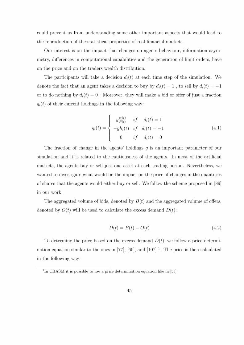
could prevent us from understanding some other important aspects that would lead to
the reproduction of the statistical properties of real financial markets.
Our interest is on the impact that changes on agents behaviour, information asym-
metry, differences in computational capabilities and the generation of limit orders, have
on the price and on the traders wealth distribution.
The participants will take a decision di(t) at each time step of the simulation. We
denote the fact that an agent takes a decision to buy by di(t) = 1 , to sell by di(t) = −1
or to do nothing by di(t) = 0 . Moreover, they will make a bid or offer of just a fraction
qi(t) of their current holdings in the following way:
qi(t) =
g ci(t)P (t)
if di(t) = 1
−ghi(t) if di(t) = −1
0 if di(t) = 0
(4.1)
The fraction of change in the agents’ holdings g is an important parameter of our
simulation and it is related to the cautiousness of the agents. In most of the artificial
markets, the agents buy or sell just one asset at each trading period. Nevertheless, we
wanted to investigate what would be the impact on the price of changes in the quantities
of shares that the agents would either buy or sell. We follow the scheme proposed in [89]
in our work.
The aggregated volume of bids, denoted by B(t) and the aggregated volume of offers,
denoted by O(t) will be used to calculate the excess demand D(t):
D(t) = B(t)−O(t) (4.2)
To determine the price based on the excess demand D(t), we follow a price determi-
nation equation similar to the ones in [77], [60], and [107] 1. The price is then calculated
in the following way:
1In CHASM it is possible to use a price determination equation like in [53]
45
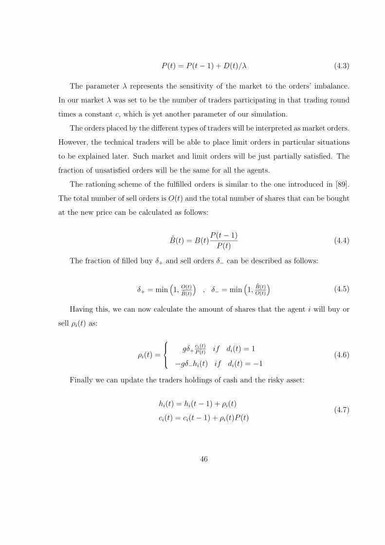
P (t) = P (t− 1) + D(t)/λ (4.3)
The parameter λ represents the sensitivity of the market to the orders’ imbalance.
In our market λ was set to be the number of traders participating in that trading round
times a constant c, which is yet another parameter of our simulation.
The orders placed by the different types of traders will be interpreted as market orders.
However, the technical traders will be able to place limit orders in particular situations
to be explained later. Such market and limit orders will be just partially satisfied. The
fraction of unsatisfied orders will be the same for all the agents.
The rationing scheme of the fulfilled orders is similar to the one introduced in [89].
The total number of sell orders is O(t) and the total number of shares that can be bought
at the new price can be calculated as follows:
B(t) = B(t)P (t− 1)
P (t)(4.4)
The fraction of filled buy δ+ and sell orders δ− can be described as follows:
δ+ = min(1, O(t)
B(t)
), δ− = min
(1, B(t)
O(t)
)(4.5)
Having this, we can now calculate the amount of shares that the agent i will buy or
sell ρi(t) as:
ρi(t) =
gδ+ci(t)P (t)
if di(t) = 1
−gδ−hi(t) if di(t) = −1(4.6)
Finally we can update the traders holdings of cash and the risky asset:
hi(t) = hi(t− 1) + ρi(t)
ci(t) = ci(t− 1) + ρi(t)P (t)(4.7)
46
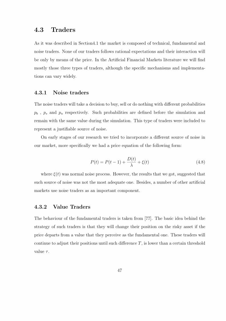
4.3 Traders
As it was described in Section4.1 the market is composed of technical, fundamental and
noise traders. None of our traders follows rational expectations and their interaction will
be only by means of the price. In the Artificial Financial Markets literature we will find
mostly those three types of traders, although the specific mechanisms and implementa-
tions can vary widely.
4.3.1 Noise traders
The noise traders will take a decision to buy, sell or do nothing with different probabilities
pb , ps and pn respectively. Such probabilities are defined before the simulation and
remain with the same value during the simulation. This type of traders were included to
represent a justifiable source of noise.
On early stages of our research we tried to incorporate a different source of noise in
our market, more specifically we had a price equation of the following form:
P (t) = P (t− 1) +D(t)
λ+ ξ(t) (4.8)
where ξ(t) was normal noise process. However, the results that we got, suggested that
such source of noise was not the most adequate one. Besides, a number of other artificial
markets use noise traders as an important component.
4.3.2 Value Traders
The behaviour of the fundamental traders is taken from [77]. The basic idea behind the
strategy of such traders is that they will change their position on the risky asset if the
price departs from a value that they perceive as the fundamental one. These traders will
continue to adjust their positions until such difference T , is lower than a certain threshold
value τ .
47
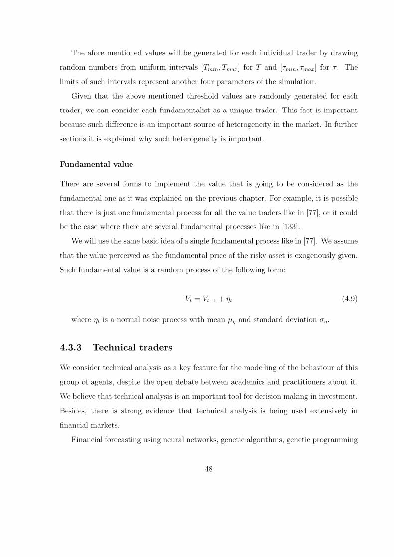
The afore mentioned values will be generated for each individual trader by drawing
random numbers from uniform intervals [Tmin, Tmax] for T and [τmin, τmax] for τ . The
limits of such intervals represent another four parameters of the simulation.
Given that the above mentioned threshold values are randomly generated for each
trader, we can consider each fundamentalist as a unique trader. This fact is important
because such difference is an important source of heterogeneity in the market. In further
sections it is explained why such heterogeneity is important.
Fundamental value
There are several forms to implement the value that is going to be considered as the
fundamental one as it was explained on the previous chapter. For example, it is possible
that there is just one fundamental process for all the value traders like in [77], or it could
be the case where there are several fundamental processes like in [133].
We will use the same basic idea of a single fundamental process like in [77]. We assume
that the value perceived as the fundamental price of the risky asset is exogenously given.
Such fundamental value is a random process of the following form:
Vt = Vt−1 + ηt (4.9)
where ηt is a normal noise process with mean µη and standard deviation ση.
4.3.3 Technical traders
We consider technical analysis as a key feature for the modelling of the behaviour of this
group of agents, despite the open debate between academics and practitioners about it.
We believe that technical analysis is an important tool for decision making in investment.
Besides, there is strong evidence that technical analysis is being used extensively in
financial markets.
Financial forecasting using neural networks, genetic algorithms, genetic programming
48

and other machine learning techniques has been a very dynamic field of study. We can
see some important work in the nineties and some innovative recent proposals [5], [18],
[19], [29], [41], [61], [63], [64], [62], [84], [83], [85], [195]. An always increasing number of
works testify the interest of the researchers and the financial industry on this buoyant
area.
Broadly speaking, the technical traders in our artificial market forecast if the price
is going to rise by a certain r% within a certain n number of days. For that purpose,
they will be equipped with up to twelve different technical and momentum indicators
to form investment decision rules. Such indicators are well known technical indicators.
We chose a short period indicator and a long period one because it is the way in which
they are used by technical analysts. We will give more detail regarding the indicators in
subsection 4.6.3.
Each technical trader owns a population of such investment decision rules, represented
by decision trees. The decision trees are randomly initialized and then evolved by an
evolutionary mechanism known as Genetic Programming (GP) [113], [117]. EDDIE ([41],
[195], [131], [194], [196], [148], [199], [197]) constitutes the basic platform to the design
of the investment strategy of this group of agents.
Genetic programming has been used in the past to model agents in artificial financial
markets [69], [68], [211], [53], [48] and [149].
It is important to point out that the agents could use any kind of financial information,
even including information considered as fundamental. However, we did not want to have
many exogenous sources of information and we decided to let the traders build their own
decision rules with technical and momentum indicators, considering that we were able
to generate them all just by using the price. Additionally, under certain (exogenous)
circumstances they will be able to behave like the fundamentalists.
This group of traders is the richest in behaviour and the most complex of the market
participants. Such traders are organized in heterogeneous groups and the agents inside
each group share all the same parameters. The heterogeneity among the groups will
49
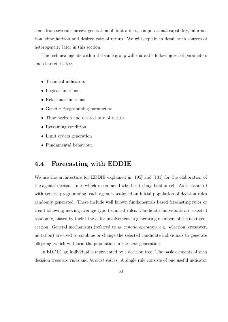
come from several sources: generation of limit orders, computational capability, informa-
tion, time horizon and desired rate of return. We will explain in detail such sources of
heterogeneity later in this section.
The technical agents within the same group will share the following set of parameters
and characteristics:
• Technical indicators
• Logical functions
• Relational functions
• Genetic Programming parameters
• Time horizon and desired rate of return
• Retraining condition
• Limit orders generation
• Fundamental behaviour.
4.4 Forecasting with EDDIE
We use the architecture for EDDIE explained in [195] and [131] for the elaboration of
the agents’ decision rules which recommend whether to buy, hold or sell. As is standard
with genetic programming, each agent is assigned an initial population of decision rules
randomly generated. These include well known fundamentals based forecasting rules or
trend following moving average type technical rules. Candidate individuals are selected
randomly, biased by their fitness, for involvement in generating members of the next gen-
eration. General mechanisms (referred to as genetic operators, e.g. selection, crossover,
mutation) are used to combine or change the selected candidate individuals to generate
offspring, which will form the population in the next generation.
In EDDIE, an individual is represented by a decision tree. The basic elements of such
decision trees are rules and forecast values. A single rule consists of one useful indicator
50
Figure 4-1: Example of a decision tree.
for prediction, one relational operator such as “greater than”, or “less than”, etc, and a
threshold (real value). Such a single rule interacts with other rules in one decision tree
through logic operators such as “Or”, “And”, “Not”, and “If-Then-Else”. Forecast values
in this model are directions of price movements, either a positive trend (i.e. positive x%
return within specified time interval can be achievable) or negative trend (i.e. negative
x% return within a specified time interval can be achievable).
Figure 4.4 shows an example of one possible decision tree. In such figure we can see
that the root node is always an If-Then-Else node, the left child an If-Then-Else node is
a “condition” node. Additionally, there are two right children which could be either a
“decision” node or another If-Then-Else node. The rule that is being represented by the
decision tree in Figure 4.4 is the following one:
One of the conditions of the previous expression that specifies that the moving average
of the past twelve days should be equal to 0.98 in fact is verified in a range around
such value. It would be extremely unlikely that a randomly generated number could be
matched exactly by the evolution process and for that reason a range is used instead.
The type of node is going to become relevant when applying the crossover and muta-
51

1 If ((MA 12 = 0.98)AND(NOT (TRB 5 < 0.25))) Then2 Buy3 Else4 If(V OL 12 > 0.56) Then5 Sell6 Else7 Hold8 End if9 End if
Figure 4-2: Example of a decision rule interpreted from a decision tree
tion genetic operators because it is precise to maintain the tree consistency. For example,
in the case that a mutation operation is going to take place and the selected node where
such mutation is going to happen is a “condition” node; then, the randomly generated
mutation must be a “condition” like node. The same should happen for the crossover op-
eration: there must be compatibility between the subtrees that are going to be exchanged
by the parents.
Recommendation to BUY at t follows from the prediction of a price rise (positive
trend) over a given period, recommendation to do nothing (HOLD) follows from the fact
that there is no evidence of a price rise or a price drop and recommendation to SELL
follows from the prediction of a price fall (x% negative trend). Note different returns
thresholds and horizons exist for different classes of traders. Since decision trees are
used to predict directions of price changes and make recommendations for trade, the
success or failure of recommendations can be categorized as a three-class classification
problem. Each prediction point for every decision tree can be classified into either a
positive position, a holding position or a negative position. For each decision tree, we
define RC (Rate of Correctness), and RF (Rate of Failure) as its prediction performance
criteria. Formula for each criterion is given through a contingency table in Table 4.1 as
follows:
Lets define: RC as the Rate of Correctness; and RF as the Rate of Failure.
52
Table 4.1: A contingency table for three-class classification/prediction problem
Predicted Predicted Predictedprice rise no inf. price drop
(PBs) (PHs) (PSs)BUY HOLD SELL
Actual # of True # of Actual Buy # Actual Buyprice rise Buys Predicted Hold Predicted Sell(ABs)BUY (TB) (ABPH) (ABPS)Actual # of Actual Hold # of True # of Actual Holdno inf. Predicted Buy Holds Predicted Sell(AHs)HOLD (AHPB) (TH) (AHPS)Actual # of Actual Sell # of Actual Sell # of Trueprice drop Predicted Buy Predicted Hold Sells(ASs)SELL (ASPB) (ASPH) (TS)
RC =TB + TH + TS
ABs + AHs + ASs(4.10)
RF =AHPB + ASPB
PBs+
ABPH + ASPH
PHs+
ABPS + AHPS
PSs(4.11)
Each agent selects the decision tree which constitute trading strategy to buy or sell
that maximizes the fitness function
Γ(1) = ϕ(rc)RC − ϕ(rf)RF (4.12)
The fitness function involves two performance values, i.e. RC and RF, each of which
is assigned a different weight ϕ(rc) or ϕ(rf) respectively. While the fitness function can
guard against loss making positions, the population of decision trees from which agents
conduct their search may lead to investment income under-performance. One important
advantage of genetic programming is that we can bias the search mechanism by using
different values for such weights. However, we used a value of zero for the weight ϕ(rf).
53
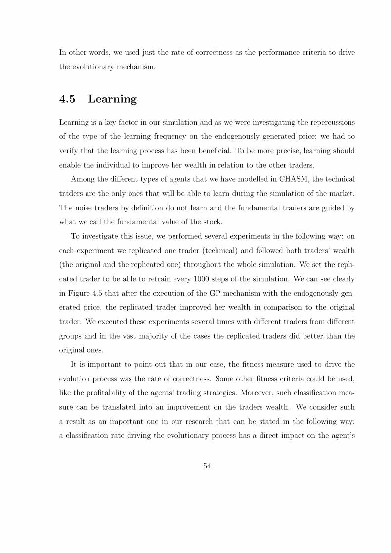
In other words, we used just the rate of correctness as the performance criteria to drive
the evolutionary mechanism.
4.5 Learning
Learning is a key factor in our simulation and as we were investigating the repercussions
of the type of the learning frequency on the endogenously generated price; we had to
verify that the learning process has been beneficial. To be more precise, learning should
enable the individual to improve her wealth in relation to the other traders.
Among the different types of agents that we have modelled in CHASM, the technical
traders are the only ones that will be able to learn during the simulation of the market.
The noise traders by definition do not learn and the fundamental traders are guided by
what we call the fundamental value of the stock.
To investigate this issue, we performed several experiments in the following way: on
each experiment we replicated one trader (technical) and followed both traders’ wealth
(the original and the replicated one) throughout the whole simulation. We set the repli-
cated trader to be able to retrain every 1000 steps of the simulation. We can see clearly
in Figure 4.5 that after the execution of the GP mechanism with the endogenously gen-
erated price, the replicated trader improved her wealth in comparison to the original
trader. We executed these experiments several times with different traders from different
groups and in the vast majority of the cases the replicated traders did better than the
original ones.
It is important to point out that in our case, the fitness measure used to drive the
evolution process was the rate of correctness. Some other fitness criteria could be used,
like the profitability of the agents’ trading strategies. Moreover, such classification mea-
sure can be translated into an improvement on the traders wealth. We consider such
a result as an important one in our research that can be stated in the following way:
a classification rate driving the evolutionary process has a direct impact on the agent’s
54
0 1000 2000 3000 4000 50000
0.5
1
1.5
2
2.5
3
3.5x 10
5
OriginalRetrained
(a)
0 1000 2000 3000 4000 50000.6
0.7
0.8
0.9
1
1.1
1.2
1.3
1.4x 10
5
OriginalRetrained
(b)
0 1000 2000 3000 4000 50000.9
0.95
1
1.05
1.1
1.15
1.2
1.25
1.3
1.35x 10
5
OriginalRetrained
(c)
0 500 1000 1500 2000 2500 30000.95
1
1.05
1.1
1.15
1.2
1.25
1.3x 10
5
OriginalRetrained
(d)
Figure 4-3: Examples of wealth evolution with (red dashed line) and without learning(blue continuous line).
55
wealth. It is not obvious that a better classification rate leads to a better application
performance. Fortunately, in our case this is true.
4.6 Important Characteristics of CHASM
In this section we will describe in detail some of the most important features of CHASM.
The implications of changes in such important aspects of our model will be described by
experimentation in the next chapter.
4.6.1 Market and limit orders
When a person, a professional trader, a market maker or a corporation are trading on
a stock market, there are different ways to do so. After the decision making process of
any of such entities an order must be submitted to a broker (or the representant that is
trading on behalf of them). Essentially 2, there are two main types of orders:
• Market orders
• Limit orders
The market orders are buying or selling orders that must be executed at the current
price of the stock on the market. There is certainty about the execution of a market order
but uncertainty about the execution price. On the other hand, limit orders are buying
or selling orders in which the trader specifies the price at which she is willing to trade
(such prices are called bid or ask prices). In the case of limit orders, there is certainty
about the execution price, but there is no certainty about the execution of the order.
In order to have a complete and realistic investment strategy, we incorporated certain
types of limit orders in addition to the market orders to model an exit strategy for the
agents. In CHASM, there are basically two types of limit orders: profit taking limit
orders and stop loss limit orders.
2there is a number of other types of orders, but it is not our intention to give a full account of them
56

The profit taking limit orders are orders for selling that are sent after a purchase
of a stock takes place. The asking price for such limit orders must be higher than the
purchasing price that originated the profit taking limit order. The basic idea behind such
order is to lock a certain profit realization for the trader. However, there is no certainty
of the execution of such type of orders.
The stop loss limit orders are orders for selling a stock that is being held by an investor.
Such order becomes a market order after the price is at or goes below a threshold price
(stop price) defined by the investor. The basic idea behind such limit orders is to try to
limit the loss of an investment made by the trader.
The profit taking limit orders are incorporated in our model to provide the agents’
with a complete investment strategy. To be more specific, if the agent forecasts that the
price is going to rise and he buys now a certain amount of shares, she would have to sell
them whenever the price actually reaches such forecasted increase. On the other hand, if
the price does not rise beyond her forecast she should sell at the end of her time horizon
due to budget constraints.
The stop loss limit orders are incorporated as well as part of an exit strategy for our
agents. The generation of such orders and the profit taking ones during the trading has
important repercussions on the dynamics and the statistical properties of the price as we
will see on the experiments reported in the next section.
4.6.2 Fundamental trading
In addition to the incorporation into the market of fundamental traders, CHASM al-
lows us to incorporate fundamental like behaviour on top of the technical traders. This
characteristic of the technical traders in our model can be justified by arguing that in
real life some traders do use technical analysis in conjunction with fundamental analysis.
These traders know that the price of a certain stock is well beyond a reasonable value
(fundamental value); however, they still follow the trend a little bit longer (short time
horizon) in order to make a profit out of it. In [186] the authors report that more than
57
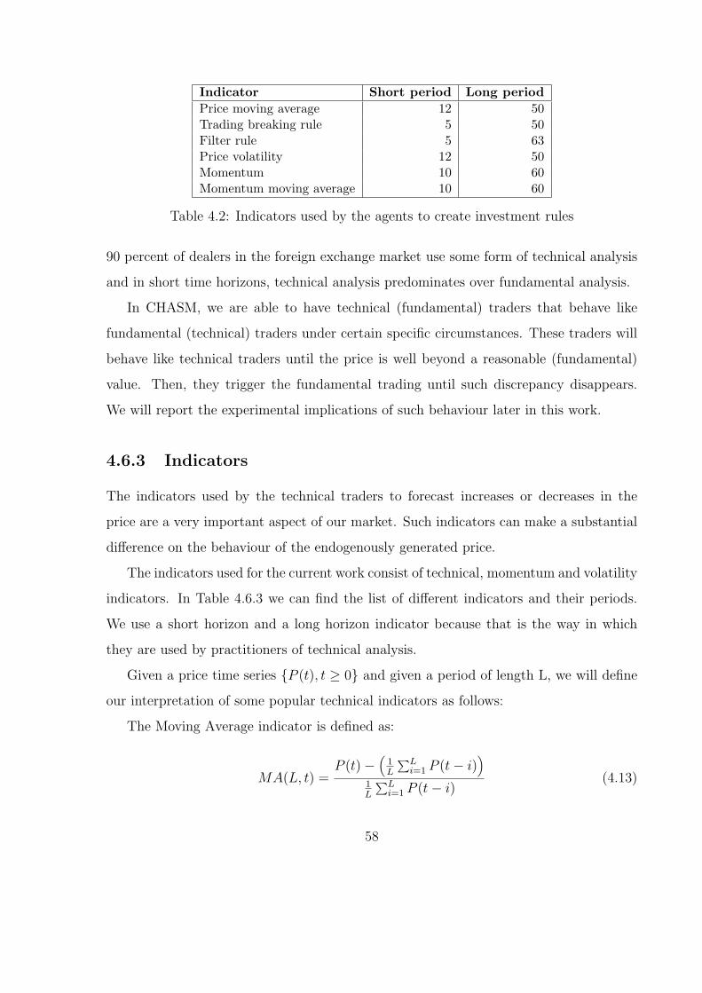
Indicator Short period Long periodPrice moving average 12 50Trading breaking rule 5 50Filter rule 5 63Price volatility 12 50Momentum 10 60Momentum moving average 10 60
Table 4.2: Indicators used by the agents to create investment rules
90 percent of dealers in the foreign exchange market use some form of technical analysis
and in short time horizons, technical analysis predominates over fundamental analysis.
In CHASM, we are able to have technical (fundamental) traders that behave like
fundamental (technical) traders under certain specific circumstances. These traders will
behave like technical traders until the price is well beyond a reasonable (fundamental)
value. Then, they trigger the fundamental trading until such discrepancy disappears.
We will report the experimental implications of such behaviour later in this work.
4.6.3 Indicators
The indicators used by the technical traders to forecast increases or decreases in the
price are a very important aspect of our market. Such indicators can make a substantial
difference on the behaviour of the endogenously generated price.
The indicators used for the current work consist of technical, momentum and volatility
indicators. In Table 4.6.3 we can find the list of different indicators and their periods.
We use a short horizon and a long horizon indicator because that is the way in which
they are used by practitioners of technical analysis.
Given a price time series {P (t), t ≥ 0} and given a period of length L, we will define
our interpretation of some popular technical indicators as follows:
The Moving Average indicator is defined as:
MA(L, t) =P (t)−
(1L
∑Li=1 P (t− i)
)
1L
∑Li=1 P (t− i)
(4.13)
58
The Trading Breakout indicator is defined as:
TRB(L, t) =P (t)−max {P (t− 1), ..., P (t− L)}
max {P (t− 1), ..., P (t− L)} (4.14)
The Filter indicator is defined as:
Filter(L, t) =P (t)−min {P (t− 1), ..., P (t− L)}
min {P (t− 1), ..., P (t− L)} (4.15)
The Volatility indicator is defined as:
V ol(L, t) =σ (P (t), ..., P (t− L + 1))
1L
∑Li=1 P (t− i)
(4.16)
where σ, represents the standard deviation.
The Momentum indicator is defined as:
Mom(L, t) = P (t)− P (t− L) (4.17)
The Moving Average Momentum indicator is defined as:
MomMA(L, t) =1
L
L∑
i=1
Mom(L, t− i) (4.18)
We chose such indicators mainly because they proved to be useful to develop invest-
ment decision rules to forecast rises and drops of the price in previous works like [5], [19],
[84], [83] and [85]. However, due to the design of the forecasting mechanism, there is
no reason to stop us using some other information like information from the limit order
book, market microstructure information, fundamental information, etc. Additionally,
we performed a sort of standardization in order to avoid that the range of numbers,
generated by the GP mechanism, to be very large and therefore increasing the size of the
search space.
There are some different ways in which the moving averages could be built (like
59
exponential moving averages) for providing the input to the forecasting mechanism. The
advantage of the exponential moving average in comparison with simple moving average
is that the later tends to signal twice for the outlying data. Nevertheless, our work is not
designed to provide the ultimate and most novel techniques in financial forecasting.
Further in this work we will explore experimentally the implications of changes on
the information (modelled here by the above listed indicators) provided to the different
groups of technical traders.
4.6.4 Computational Capability
In CHASM we model the computational capability of the agents mainly on the basis of
the GP mechanism. The two most important parameters that would determine the level
of intelligence of the agents are:
• The population size
• The number of generations.
Such parameters of the GP mechanism determine the intensity of the search engine
to look for new investment rules. If the population size is rather small then, the search
over the set of investment rules will be severely limited giving us as a result rather poor
investment rules. On the other hand, if the number of generations is small then, the
evolutionary mechanism will have little time to refine the search over the huge search
space and as result we will have again rather poor investment rules.
We will further describe the implications of variations on the computational capability
provided to the different groups of agents by the experiments described in the next
chapter.
4.6.5 Desired return and time horizon
The technical traders will be organized in groups that will share common characteristics,
as it has been described previously. Among such characteristics we have the desired rate
60
of return and the corresponding time horizon to achieve such rate of return. These two
characteristics (parameters) proved to be of central importance on the behaviour of the
market, since our GP agents work as classifiers.
The majority of the simulated markets possess agents that do not consider multi-
period preferences and the agents share the same planning, forecasting and decision
making horizon [118]. CHASM is different to most of the previously designed models in
the forecasting mechanism and the heterogeneity of time horizons.
The GP forecasting mechanism of our agents works, broadly speaking, by classifying
the training cases in three different classes: buy, sell or hold. Such classification depends
on the time horizon provided as the mechanism verifies for each data point if in the near
future (time horizon) effectively, there was a rise (drop) on the price by more (less) than
the desired rate of return.
If the selection of such quantities is unreasonable, it will cause the classifier to be
biased towards a certain class. Therefore, creating unrealistic (unreasonable) investment
rules and having an unrealistic price and statistical properties of the returns.
The next chapter describes some experiments that were designed to test the impact
that this feature of CHASM has on the dynamics of the simulation.
4.6.6 Trading proportion
The trading proportion is a parameter of the market that controls the proportion of the
asset or cash that the traders would commit on each of the operations that they will
perform during the trading rounds. Such trading proportion is a quantity that we can
use to model the degree of cautiousness of the agents in our market.
The trading proportion proved to be of central importance in our simulations. The
implications of this important feature of our market will be tested experimentally and
described in the next chapter.
61

4.6.7 Fitness function
The fitness function is a very important aspect of our market, we use a prediction accuracy
fitness function to drive the GP mechanisms of each of the agents. The fitness function
used as a rate of accuracy was the rate of correctness defined as the number of correct
classification over the total number of cases. The memory of the traders is going to be
of the same size as the size used for the initial training. There exists the possibility of
using some other ingredients (like the rate of failure) on the fitness functions to bias the
search over the solution space. Some interesting changes to the fitness measure have been
implemented and tested in [132].
The flexibility on the manipulation of the fitness function due to the original design of
the GP forecasting mechanism is one of the main advantages that we consider important
in the use of GP as a successful technique to perform financial forecasting.
4.7 CHASM: The software
In this section we will briefly describe CHASM from the Software engineering point of
view. We will describe its main components and we will explain the reasons why such
platform can be easily extended to test different economic hypotheses.
4.7.1 Design
From the very beginning, the software was designed having in mind the following desired
properties:
• The software should be easy to modify in order to incorporate some new features
• The software should be easy to extend to include some new functionalities
• The software should be highly parameterized in order to allow the user to executedifferent scenarios.
62
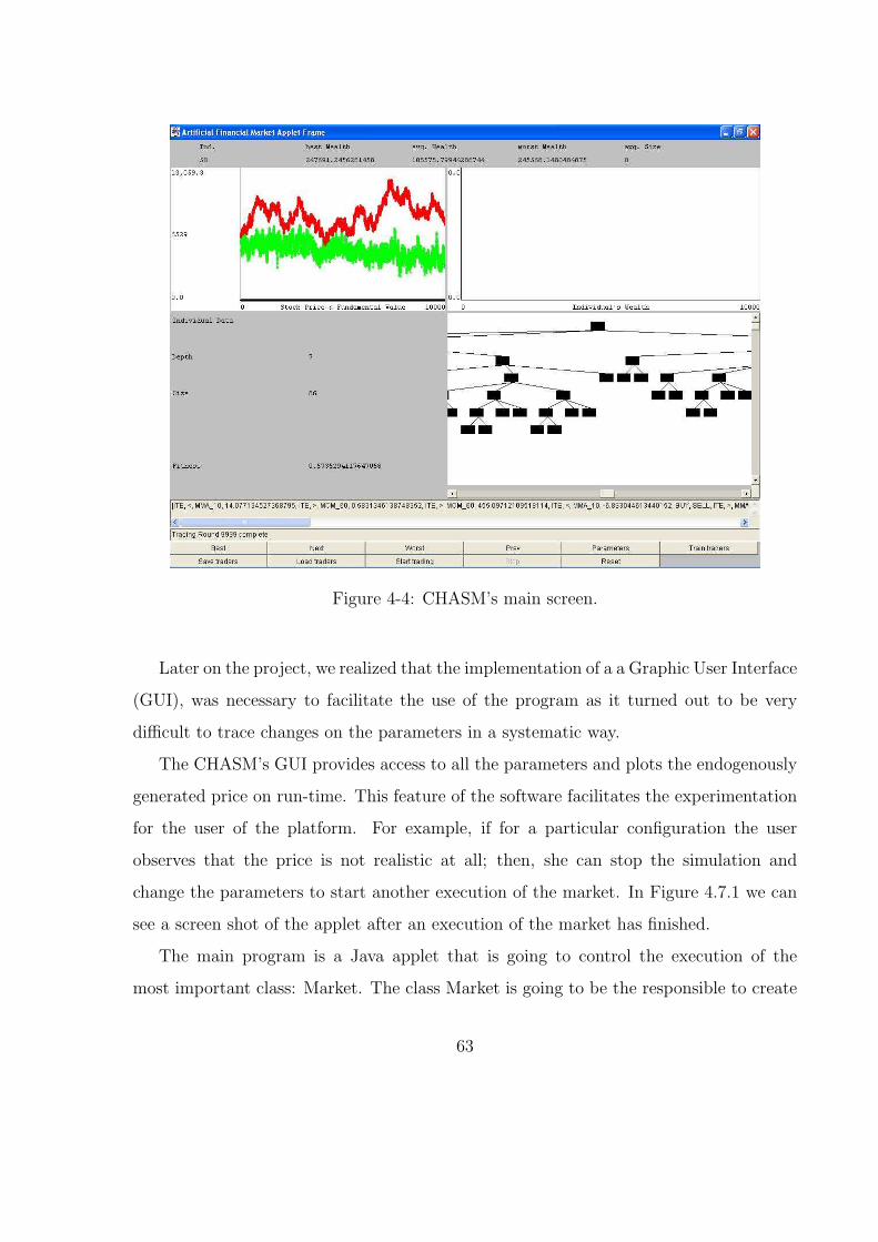
Figure 4-4: CHASM’s main screen.
Later on the project, we realized that the implementation of a a Graphic User Interface
(GUI), was necessary to facilitate the use of the program as it turned out to be very
difficult to trace changes on the parameters in a systematic way.
The CHASM’s GUI provides access to all the parameters and plots the endogenously
generated price on run-time. This feature of the software facilitates the experimentation
for the user of the platform. For example, if for a particular configuration the user
observes that the price is not realistic at all; then, she can stop the simulation and
change the parameters to start another execution of the market. In Figure 4.7.1 we can
see a screen shot of the applet after an execution of the market has finished.
The main program is a Java applet that is going to control the execution of the
most important class: Market. The class Market is going to be the responsible to create
63

Figure 4-5: CHASM java classes.
and maintain all the agents. Additionally, such class is going to store all the necessary
statistics for further analysis and is going to assure market clearing. In Figure 4.7.1 we
can observe CHASM’s most important classes and their organization.
We based the design of the agents that behave like technical traders mainly on EDDIE
[131], [195], [194] and [196]. In Figure 4.7.1 we can observe the TechnicalTrader java
class and its main components. It is worth saying, that such class is going to run a GP
mechanism (an EDDIE like mechanism). This means that each technical trader possesses
a forecasting mechanism and that is the reason why our market can be considered a
Multiple Population Genetic Programming (MP GP) market.
CHASM will write on text files several output files in order to allow further analysis
of the execution of the market. In addition to the endogenously generated price and
corresponding indicators, the platform is going to generate output for the three different
types of traders for each trading round. Finally, the market is going to generate a text
file with the following information for each trading round:
64
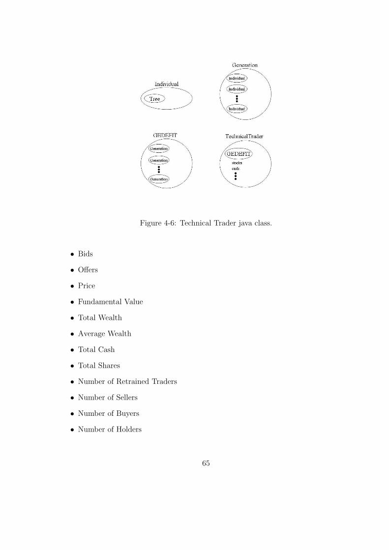
Figure 4-6: Technical Trader java class.
• Bids
• Offers
• Price
• Fundamental Value
• Total Wealth
• Average Wealth
• Total Cash
• Total Shares
• Number of Retrained Traders
• Number of Sellers
• Number of Buyers
• Number of Holders
65
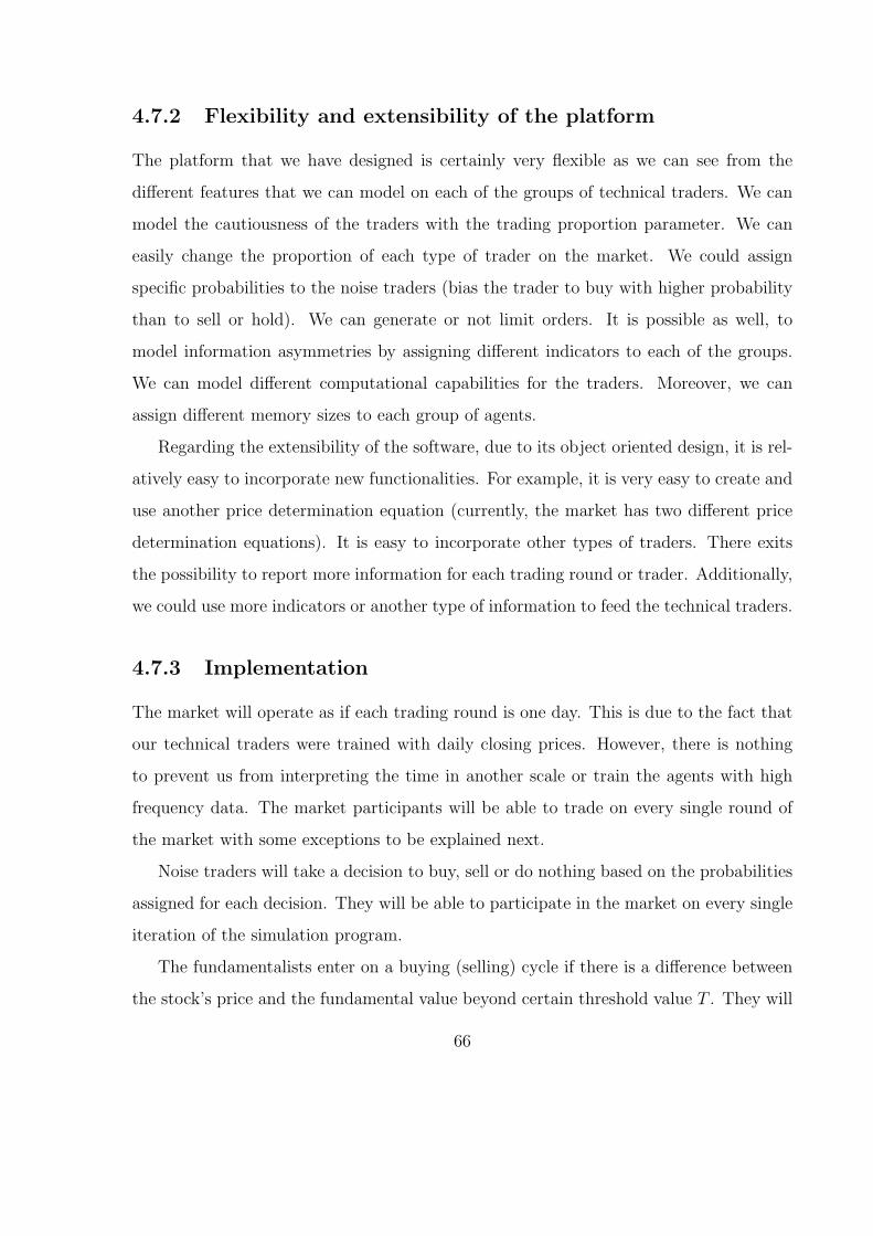
4.7.2 Flexibility and extensibility of the platform
The platform that we have designed is certainly very flexible as we can see from the
different features that we can model on each of the groups of technical traders. We can
model the cautiousness of the traders with the trading proportion parameter. We can
easily change the proportion of each type of trader on the market. We could assign
specific probabilities to the noise traders (bias the trader to buy with higher probability
than to sell or hold). We can generate or not limit orders. It is possible as well, to
model information asymmetries by assigning different indicators to each of the groups.
We can model different computational capabilities for the traders. Moreover, we can
assign different memory sizes to each group of agents.
Regarding the extensibility of the software, due to its object oriented design, it is rel-
atively easy to incorporate new functionalities. For example, it is very easy to create and
use another price determination equation (currently, the market has two different price
determination equations). It is easy to incorporate other types of traders. There exits
the possibility to report more information for each trading round or trader. Additionally,
we could use more indicators or another type of information to feed the technical traders.
4.7.3 Implementation
The market will operate as if each trading round is one day. This is due to the fact that
our technical traders were trained with daily closing prices. However, there is nothing
to prevent us from interpreting the time in another scale or train the agents with high
frequency data. The market participants will be able to trade on every single round of
the market with some exceptions to be explained next.
Noise traders will take a decision to buy, sell or do nothing based on the probabilities
assigned for each decision. They will be able to participate in the market on every single
iteration of the simulation program.
The fundamentalists enter on a buying (selling) cycle if there is a difference between
the stock’s price and the fundamental value beyond certain threshold value T . They will
66

stay in such cycle until the difference is smaller than another threshold value τ . After
the return of the stock’s price to the fundamental value, this type of traders will review
again if there exists a difference between the price and fundamental value and so on.
The technical traders can change their position on each trading round based on their
forecasts, unless they have some pending limit orders to execute. Once they have com-
pleted the round trip (the investment decision and the exit strategy), they can take
another decision based on the generated rules. A more complex (realistic) scheme of
investment could be implemented. For example, the agents could be allowed to take
a decision on each time period. However, the analysis of such scheme could become
impossible. For that reason, it is not uncommon to see even simpler schemes in other
works.
Once all the market participants make their bids and offers, we calculate the excess
demand and then the price can be updated. Afterwards, each agents’ orders are partially
satisfied by a proportion that clears the market considering the new price. Finally, the
holdings of the risky asset and cash are updated for each of the traders that participated
in the trading round.
After all the above steps are executed, each technical trader reviews its retraining
condition. In the model there exist two types of conditions for retraining: in fixed time
intervals and in an endogenous way known as Red Queen retraining.
In the case that the retraining periodicity is set to be in fixed time intervals, the
trader launches the GP mechanism creating the initial population of rules with half of
her current population and the other half randomly generated.
The case of the Red Queen retraining is more complex: retraining for a certain
agent will take place whenever the agent’s wealth falls below the average wealth. The
agent’s initial population for each retraining process is generated in the same way as
was described for the retraining with fixed periodicity. The implications of such forms of
retraining are going to be described in Chapter 7.
67

4.7.4 Parameters
We have created a flexible model in which we have a large number of different parameters
for us to explore and analyze different phenomena in financial markets. These parameters
are going to be divided mainly in two different classes: market parameters and traders’
parameters.
Market Parameters
The market parameters control some of the general parameters of the simulation, they
determine for example the proportion to invest, the number of periods of trading, etc.
Below is a list of the relevant market parameters:
• Number of trading periods
• Proportion to trade
• Price constants
• Random seed
In Figure 4.7.4 we can observe the parameters that are available to the user, with the
exception of the technical traders parameters’ window that is going to be shown later in
this work.
Traders’ parameters
The different types of traders possess different parameters. For example, the noise traders
only have three parameters: the probability to buy, the probability to sell and the prob-
ability to do nothing. On the other hand, the fundamentalists have four constants as
parameters: Tmin, Tmax, τmin and τmax. All the different traders share as parameters the
initial number of shares and the initial amount of cash available at the beginning of the
simulation.
68
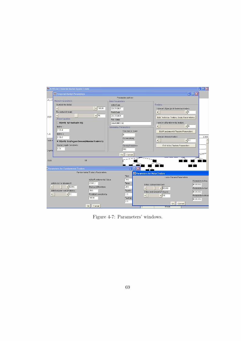
Figure 4-7: Parameters’ windows.
69

The group of technical traders is organized in several groups. Within such groups
they share the same parameters. This organization allowed us to model a key factor
in our research: heterogeneity. It is possible to split the parameters of the technical
traders in three different types: group parameters, information parameters and genetic
programming parameters.
The most important group parameters are:
• Desired rate of return
• Time horizon
• Memory length
• Retraining condition
• Fixed retraining periodicity
• Fitness function type
• Limit order to sell generation
• Limit order to buy generation
• Fundamental behaviour
• Tmin, Tmax, τmin and τmax
We used a memory length of around three years and we did not changed or scaled
it during our experiments mainly because we wanted to maintain a certain prediction
accuracy and our previous experience on this issue is that three years make a good
training data set.
The information parameters refer to the technical indicators that the agents can use
to generate the investment rules during the execution of the GP mechanism. With the
parametrization of the indicators we can model different types of technical traders. For
example, we can have moving average or momentum traders.
Within the parameters of the technical traders, the GP ones constitute an important
set for the simulation. Such parameters will determine how close to a competent trader
70

the agents are. For example, if the traders are equipped with a limited population size and
a small number of generations, there is little chance that the traders will create accurate
investment rules. The most important parameters that control the genetic programming
mechanism are:
• Population size
• Number of generations
• Mutation rate
• Crossover rate
• Initial tree depth
• Maximum tree depth
• Tournament size
• Probability of selecting the best individual of the tournament
• Tarpeian constant
In Figure 4.7.4 we can observe the parameters’ window for one of the groups of tech-
nical traders. In such window we can observe the GP related parameters, the information
parameters, the retraining conditions, the fundamental behaviour condition and the limit
orders generation options.
71
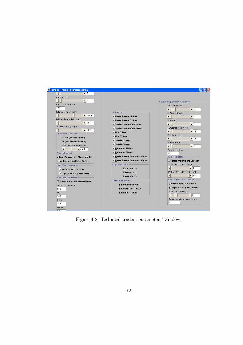
Figure 4-8: Technical traders parameters’ window.
72
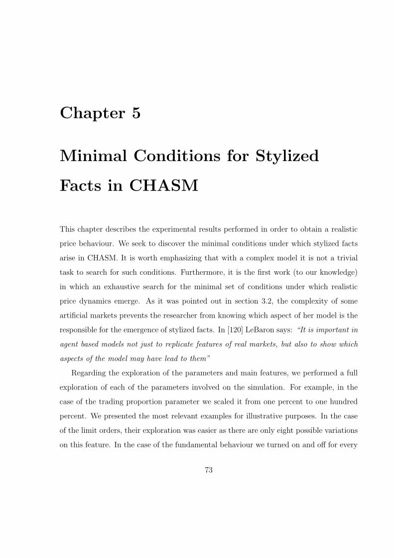
Chapter 5
Minimal Conditions for Stylized
Facts in CHASM
This chapter describes the experimental results performed in order to obtain a realistic
price behaviour. We seek to discover the minimal conditions under which stylized facts
arise in CHASM. It is worth emphasizing that with a complex model it is not a trivial
task to search for such conditions. Furthermore, it is the first work (to our knowledge)
in which an exhaustive search for the minimal set of conditions under which realistic
price dynamics emerge. As it was pointed out in section 3.2, the complexity of some
artificial markets prevents the researcher from knowing which aspect of her model is the
responsible for the emergence of stylized facts. In [120] LeBaron says: “It is important in
agent based models not just to replicate features of real markets, but also to show which
aspects of the model may have lead to them”
Regarding the exploration of the parameters and main features, we performed a full
exploration of each of the parameters involved on the simulation. For example, in the
case of the trading proportion parameter we scaled it from one percent to one hundred
percent. We presented the most relevant examples for illustrative purposes. In the case
of the limit orders, their exploration was easier as there are only eight possible variations
on this feature. In the case of the fundamental behaviour we turned on and off for every
73

single group of the technical traders. We proceeded on the same fashion for all the above
mentioned parameters and features. Nevertheless, we will only present the results of the
most relevant cases.
5.1 Parameters and features exploration
In the previous chapter we described the important characteristics and parameters of
CHASM. Due to the different possible combinations of such features and parameters,
a systematic approach was necessary to discover promising areas under which we could
obtained the desirable properties of the price.
In the following sections of this chapter we will first describe the characteristics of
what we call the base case and then, we will describe the experimental results of changes
on the other features and parameters of the model. In such case, we believe that we found
the characteristics and parameters under which a realistic price behaviour was obtained.
5.2 The base case
A large amount (one for each trader) of controlled experiments were conducted before
obtaining a price that resembles the dynamics present in real prices. In this section, we
present the results of a parameter setting which reproduce statistical properties of stock
returns. This setting will be used as a base case for studying the effects of changing the
model along individual dimensions listed in the previous chapter.
To illustrate the complexity of the parameter selection in our model we can see Figure
5-1 where we can visually contemplate the sort of prices that were generated under the
different parameter settings. We can consider the setting at the centre of picture our
basic case. In such case, in addition to the realistic looking price, the statistical properties
exhibit some of the stylized facts. From there, we explored one by one the individual
dimensions to examine the implications of changes along them.
74
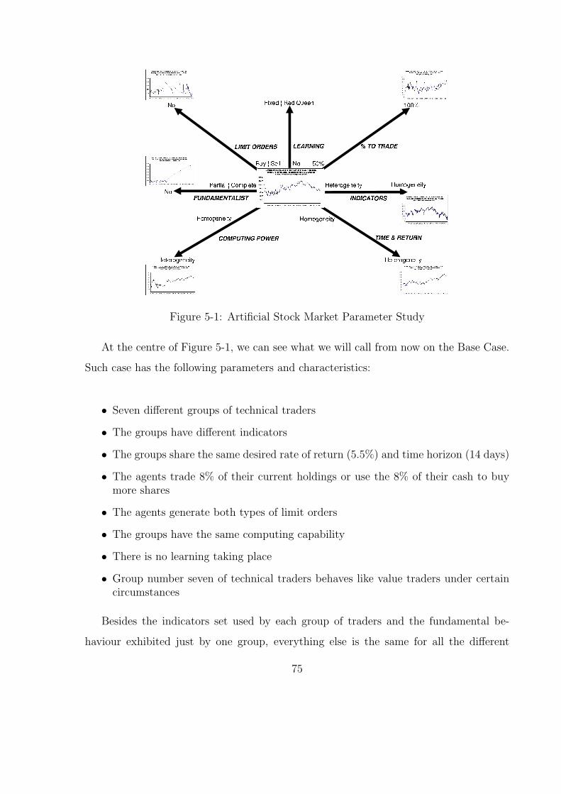
Figure 5-1: Artificial Stock Market Parameter Study
At the centre of Figure 5-1, we can see what we will call from now on the Base Case.
Such case has the following parameters and characteristics:
• Seven different groups of technical traders
• The groups have different indicators
• The groups share the same desired rate of return (5.5%) and time horizon (14 days)
• The agents trade 8% of their current holdings or use the 8% of their cash to buymore shares
• The agents generate both types of limit orders
• The groups have the same computing capability
• There is no learning taking place
• Group number seven of technical traders behaves like value traders under certaincircumstances
Besides the indicators set used by each group of traders and the fundamental be-
haviour exhibited just by one group, everything else is the same for all the different
75
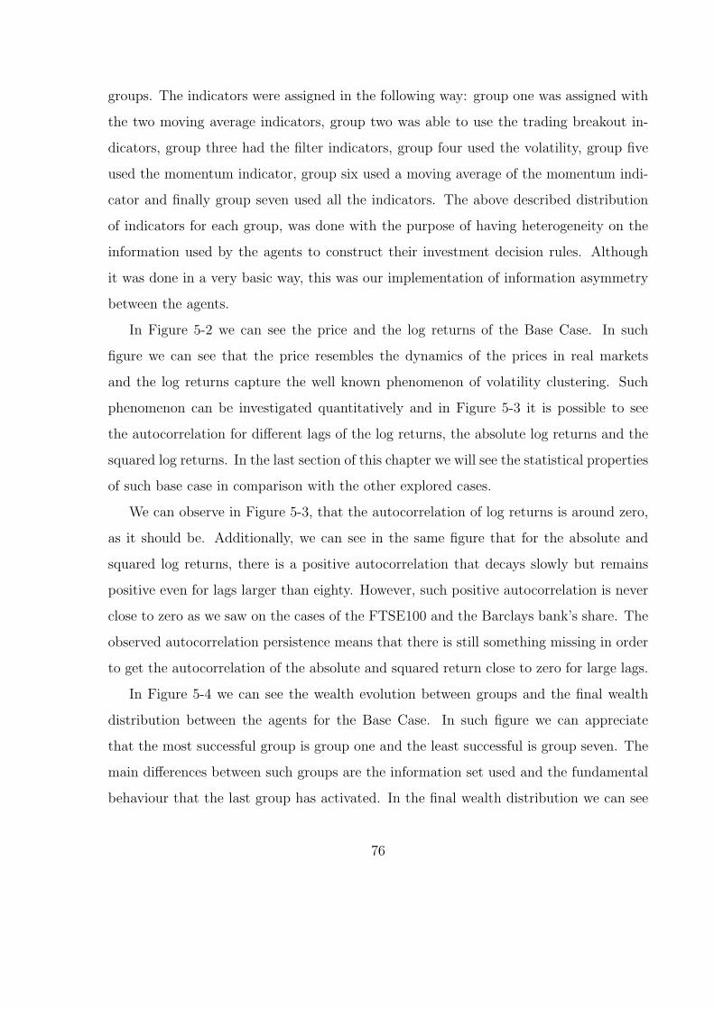
groups. The indicators were assigned in the following way: group one was assigned with
the two moving average indicators, group two was able to use the trading breakout in-
dicators, group three had the filter indicators, group four used the volatility, group five
used the momentum indicator, group six used a moving average of the momentum indi-
cator and finally group seven used all the indicators. The above described distribution
of indicators for each group, was done with the purpose of having heterogeneity on the
information used by the agents to construct their investment decision rules. Although
it was done in a very basic way, this was our implementation of information asymmetry
between the agents.
In Figure 5-2 we can see the price and the log returns of the Base Case. In such
figure we can see that the price resembles the dynamics of the prices in real markets
and the log returns capture the well known phenomenon of volatility clustering. Such
phenomenon can be investigated quantitatively and in Figure 5-3 it is possible to see
the autocorrelation for different lags of the log returns, the absolute log returns and the
squared log returns. In the last section of this chapter we will see the statistical properties
of such base case in comparison with the other explored cases.
We can observe in Figure 5-3, that the autocorrelation of log returns is around zero,
as it should be. Additionally, we can see in the same figure that for the absolute and
squared log returns, there is a positive autocorrelation that decays slowly but remains
positive even for lags larger than eighty. However, such positive autocorrelation is never
close to zero as we saw on the cases of the FTSE100 and the Barclays bank’s share. The
observed autocorrelation persistence means that there is still something missing in order
to get the autocorrelation of the absolute and squared return close to zero for large lags.
In Figure 5-4 we can see the wealth evolution between groups and the final wealth
distribution between the agents for the Base Case. In such figure we can appreciate
that the most successful group is group one and the least successful is group seven. The
main differences between such groups are the information set used and the fundamental
behaviour that the last group has activated. In the final wealth distribution we can see
76
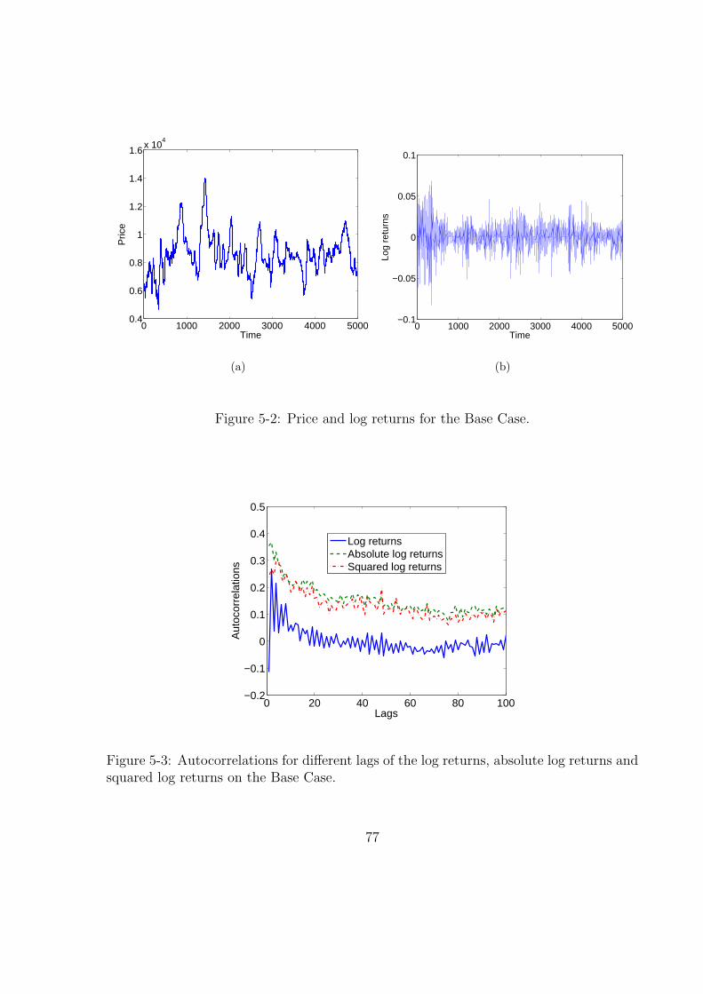
0 1000 2000 3000 4000 50000.4
0.6
0.8
1
1.2
1.4
1.6x 10
4
Time
Pric
e
(a)
0 1000 2000 3000 4000 5000−0.1
−0.05
0
0.05
0.1
Time
Log
retu
rns
(b)
Figure 5-2: Price and log returns for the Base Case.
0 20 40 60 80 100−0.2
−0.1
0
0.1
0.2
0.3
0.4
0.5
Lags
Aut
ocor
rela
tions
Log returnsAbsolute log returnsSquared log returns
Figure 5-3: Autocorrelations for different lags of the log returns, absolute log returns andsquared log returns on the Base Case.
77
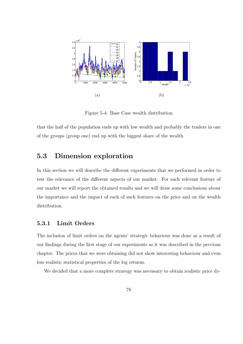
0 1000 2000 3000 4000 50001
1.2
1.4
1.6
1.8
2
2.2
2.4x 10
5
g1g2g3g4g5g6g7
(a)
0 0.5 1 1.5 2 2.5
x 106
0
0.5
1
1.5
2
2.5
3
3.5
4
Wealth
Num
ber
of T
rade
rs
(b)
Figure 5-4: Base Case wealth distribution
that the half of the population ends up with low wealth and probably the traders in one
of the groups (group one) end up with the biggest share of the wealth.
5.3 Dimension exploration
In this section we will describe the different experiments that we performed in order to
test the relevance of the different aspects of our market. For each relevant feature of
our market we will report the obtained results and we will draw some conclusions about
the importance and the impact of each of such features on the price and on the wealth
distribution.
5.3.1 Limit Orders
The inclusion of limit orders on the agents’ strategic behaviour was done as a result of
our findings during the first stage of our experiments as it was described in the previous
chapter. The prices that we were obtaining did not show interesting behaviour and even
less realistic statistical properties of the log returns.
We decided that a more complete strategy was necessary to obtain realistic price dy-
78

namics. Our agents were equipped with a powerful forecasting mechanism. Nevertheless,
after forecasting that the price would rise and buy some assets they did not realized their
profits that they would get as a reward for their forecasting ability.
The above mentioned reasons are the cause of including an exit strategy for our agents
in CHASM. Such exit strategy will be modelled by two different types of limit orders:
profit-taking limit orders and stop-loss limit orders.
Experimental design on limit orders
In order to test the relevance and the impact of the inclusion of limit orders on the agents’
trading strategy we designed some experiments in which we turned on and off the use of
one or both types of limit orders. We departed from the base case by no generating both
limit orders everything else remaining the same.
Results on limit orders
In Figure 5-5 we can see the price and the log returns of the Base Case without limit
orders being generated. We can observe by simple inspection from such figure that the
price dynamics are not realistic and that such orders represent an important element in
the generation of dynamics close to reality. It is important to stress that such orders
represent a complete investment strategy for the traders. For example, it would be
unreasonable to buy some shares today if we forecasted that the price was going to rise
and later on, keep them without realizing the profit that we could get.
We can observe under this scenario that the price has huge upwards jumps and sud-
den dramatic crashes. Additionally, after around the 4500th period, we can observe a
monotonic behaviour that is reflected on the volatility as well.
In Figure 5-6, we can observe the behaviour of the autocorrelations for different lags
of the log returns, absolute log returns and squared log returns. Considering the two
examples on Chapter 2, we can appreciate that the behaviour of the autocorrelation for
the log returns is not like in those examples (oscillating around zero). Such autocorre-
79
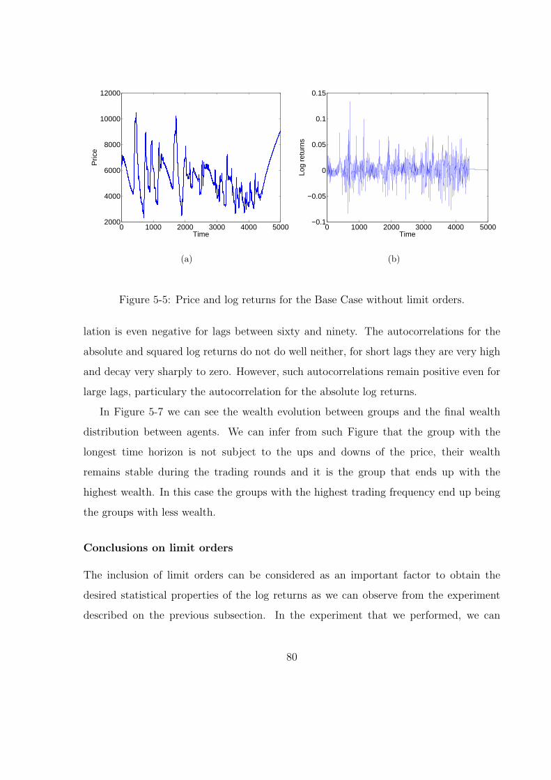
0 1000 2000 3000 4000 50002000
4000
6000
8000
10000
12000
Time
Pric
e
(a)
0 1000 2000 3000 4000 5000−0.1
−0.05
0
0.05
0.1
0.15
Time
Log
retu
rns
(b)
Figure 5-5: Price and log returns for the Base Case without limit orders.
lation is even negative for lags between sixty and ninety. The autocorrelations for the
absolute and squared log returns do not do well neither, for short lags they are very high
and decay very sharply to zero. However, such autocorrelations remain positive even for
large lags, particulary the autocorrelation for the absolute log returns.
In Figure 5-7 we can see the wealth evolution between groups and the final wealth
distribution between agents. We can infer from such Figure that the group with the
longest time horizon is not subject to the ups and downs of the price, their wealth
remains stable during the trading rounds and it is the group that ends up with the
highest wealth. In this case the groups with the highest trading frequency end up being
the groups with less wealth.
Conclusions on limit orders
The inclusion of limit orders can be considered as an important factor to obtain the
desired statistical properties of the log returns as we can observe from the experiment
described on the previous subsection. In the experiment that we performed, we can
80
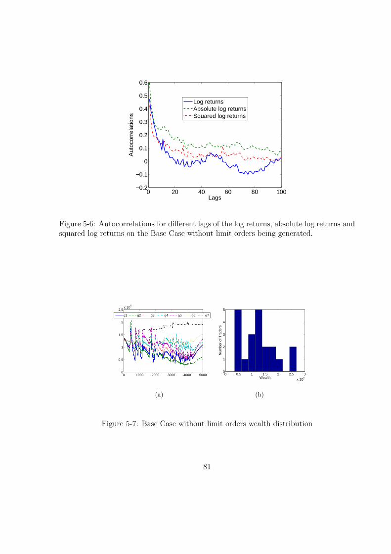
0 20 40 60 80 100−0.2
−0.1
0
0.1
0.2
0.3
0.4
0.5
0.6
Lags
Aut
ocor
rela
tions
Log returnsAbsolute log returnsSquared log returns
Figure 5-6: Autocorrelations for different lags of the log returns, absolute log returns andsquared log returns on the Base Case without limit orders being generated.
0 1000 2000 3000 4000 50000
0.5
1
1.5
2
2.5x 10
5
g1 g2 g3 g4 g5 g6 g7
(a)
0 0.5 1 1.5 2 2.5 3
x 105
0
1
2
3
4
5
Wealth
Num
ber
of T
rade
rs
(b)
Figure 5-7: Base Case without limit orders wealth distribution
81
observe that the omission of the limit orders gives as a result very unrealistic price
dynamics. We can see that the price and log returns do not behave in the way that real
prices and log returns do. The price is far from the prices in real markets and the returns
do not capture the phenomena of volatility clustering. Moreover, after a certain period,
the volatility of the returns becomes constant. Additionally, at the end of the price’s
graph we can see that there was a sort of consensus between the traders and the price
started to increase without reversion taking place. This phenomenon might be caused
by the lack of a complete investment strategy as it was explained before. In other words,
the agents were not selling to make profits after they bought with the purpose of making
some profits.
5.3.2 Fundamental trading
Fundamental behaviour is one of the aspects that most of the Artificial Financial Markets
possess. It is a very important mechanism, in our experience, in order to avoid the price
to behave in a very simplistic fashion. Before including such characteristic in our market,
we had prices that were either always increasing or decreasing until they collapsed. We
modelled the fundamental behaviour as it was designed in [77], on top of the technical
trading behaviour. This means that the agents will be trading like technical traders until
the price departs beyond a certain threshold value from what they consider to be the
fundamental value of the risky asset.
The decision to enhance the technical traders with fundamental-like behaviour is
based on the behaviour of some traders as it is reported in [186]. In such paper the
authors report that some traders acknowledged that in various occasions, although they
believed that the price was departing from the fundamental value; they would still chase
a trend (a little bit longer) in order to make a profit out of it.
82
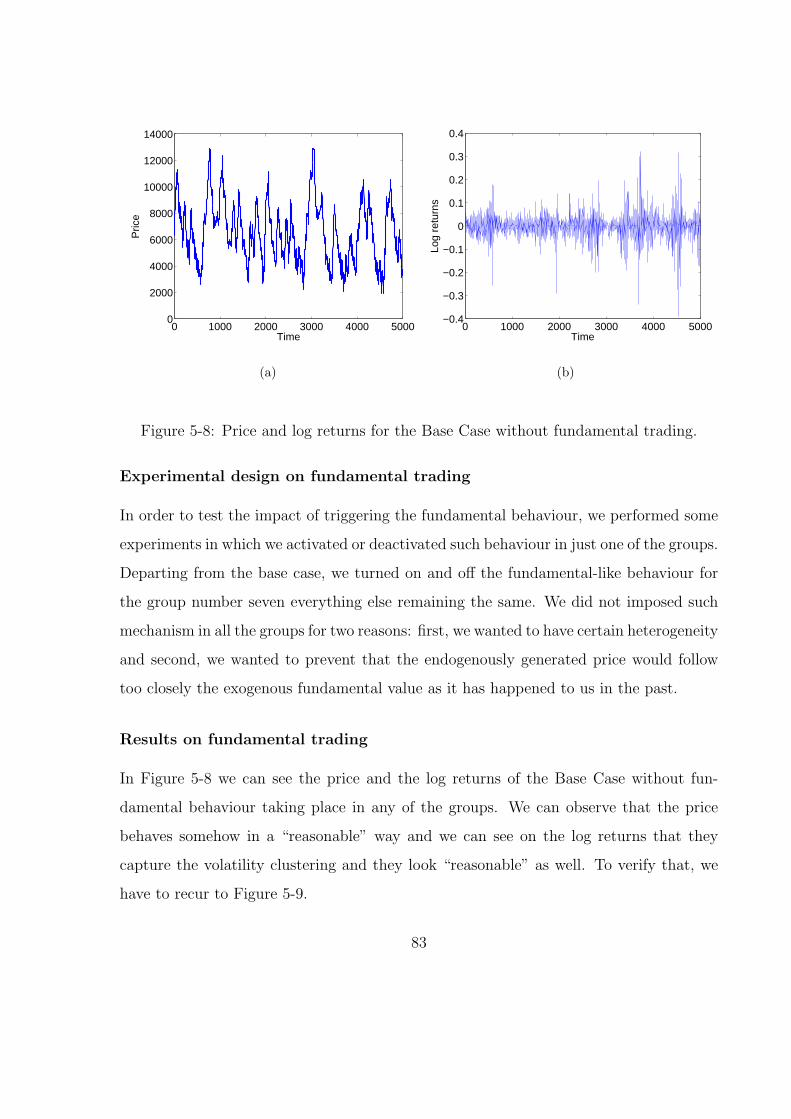
0 1000 2000 3000 4000 50000
2000
4000
6000
8000
10000
12000
14000
Time
Pric
e
(a)
0 1000 2000 3000 4000 5000−0.4
−0.3
−0.2
−0.1
0
0.1
0.2
0.3
0.4
Time
Log
retu
rns
(b)
Figure 5-8: Price and log returns for the Base Case without fundamental trading.
Experimental design on fundamental trading
In order to test the impact of triggering the fundamental behaviour, we performed some
experiments in which we activated or deactivated such behaviour in just one of the groups.
Departing from the base case, we turned on and off the fundamental-like behaviour for
the group number seven everything else remaining the same. We did not imposed such
mechanism in all the groups for two reasons: first, we wanted to have certain heterogeneity
and second, we wanted to prevent that the endogenously generated price would follow
too closely the exogenous fundamental value as it has happened to us in the past.
Results on fundamental trading
In Figure 5-8 we can see the price and the log returns of the Base Case without fun-
damental behaviour taking place in any of the groups. We can observe that the price
behaves somehow in a “reasonable” way and we can see on the log returns that they
capture the volatility clustering and they look “reasonable” as well. To verify that, we
have to recur to Figure 5-9.
83
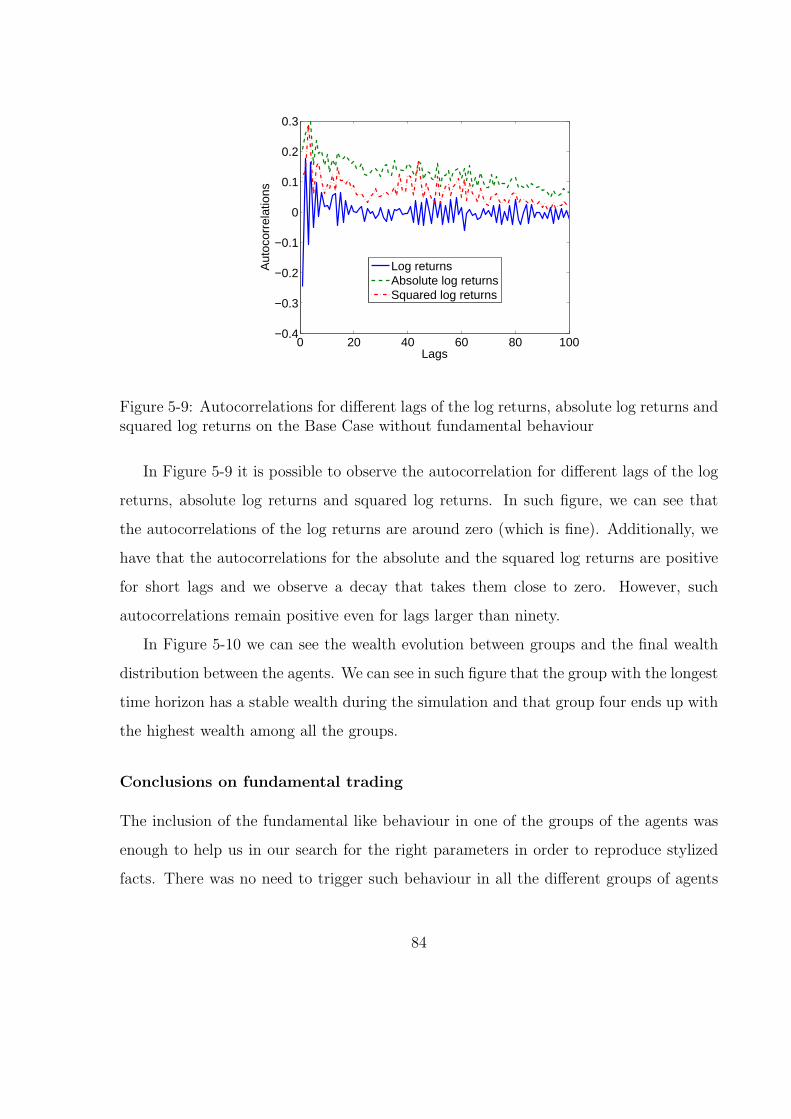
0 20 40 60 80 100−0.4
−0.3
−0.2
−0.1
0
0.1
0.2
0.3
Lags
Aut
ocor
rela
tions
Log returnsAbsolute log returnsSquared log returns
Figure 5-9: Autocorrelations for different lags of the log returns, absolute log returns andsquared log returns on the Base Case without fundamental behaviour
In Figure 5-9 it is possible to observe the autocorrelation for different lags of the log
returns, absolute log returns and squared log returns. In such figure, we can see that
the autocorrelations of the log returns are around zero (which is fine). Additionally, we
have that the autocorrelations for the absolute and the squared log returns are positive
for short lags and we observe a decay that takes them close to zero. However, such
autocorrelations remain positive even for lags larger than ninety.
In Figure 5-10 we can see the wealth evolution between groups and the final wealth
distribution between the agents. We can see in such figure that the group with the longest
time horizon has a stable wealth during the simulation and that group four ends up with
the highest wealth among all the groups.
Conclusions on fundamental trading
The inclusion of the fundamental like behaviour in one of the groups of the agents was
enough to help us in our search for the right parameters in order to reproduce stylized
facts. There was no need to trigger such behaviour in all the different groups of agents
84
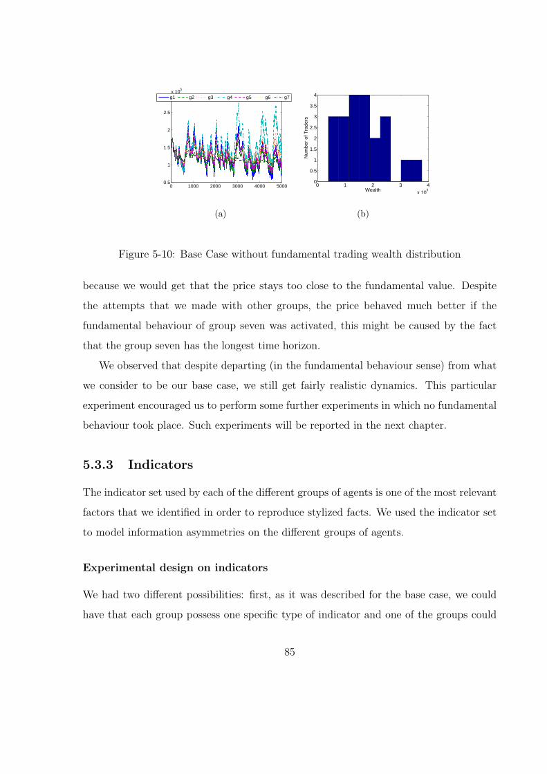
0 1000 2000 3000 4000 50000.5
1
1.5
2
2.5
3x 10
5
g1 g2 g3 g4 g5 g6 g7
(a)
0 1 2 3 4
x 105
0
0.5
1
1.5
2
2.5
3
3.5
4
Wealth
Num
ber
of T
rade
rs
(b)
Figure 5-10: Base Case without fundamental trading wealth distribution
because we would get that the price stays too close to the fundamental value. Despite
the attempts that we made with other groups, the price behaved much better if the
fundamental behaviour of group seven was activated, this might be caused by the fact
that the group seven has the longest time horizon.
We observed that despite departing (in the fundamental behaviour sense) from what
we consider to be our base case, we still get fairly realistic dynamics. This particular
experiment encouraged us to perform some further experiments in which no fundamental
behaviour took place. Such experiments will be reported in the next chapter.
5.3.3 Indicators
The indicator set used by each of the different groups of agents is one of the most relevant
factors that we identified in order to reproduce stylized facts. We used the indicator set
to model information asymmetries on the different groups of agents.
Experimental design on indicators
We had two different possibilities: first, as it was described for the base case, we could
have that each group possess one specific type of indicator and one of the groups could
85
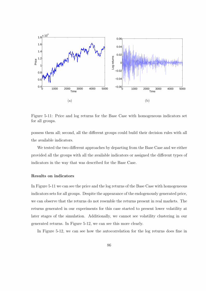
0 1000 2000 3000 4000 50000.4
0.6
0.8
1
1.2
1.4
1.6
1.8x 10
4
Time
Pric
e
(a)
0 1000 2000 3000 4000 5000−0.06
−0.04
−0.02
0
0.02
0.04
0.06
Time
Log
retu
rns
(b)
Figure 5-11: Price and log returns for the Base Case with homogeneous indicators setfor all groups.
possess them all; second, all the different groups could build their decision rules with all
the available indicators.
We tested the two different approaches by departing from the Base Case and we either
provided all the groups with all the available indicators or assigned the different types of
indicators in the way that was described for the Base Case.
Results on indicators
In Figure 5-11 we can see the price and the log returns of the Base Case with homogeneous
indicators sets for all groups. Despite the appearance of the endogenously generated price,
we can observe that the returns do not resemble the returns present in real markets. The
returns generated in our experiments for this case started to present lower volatility at
later stages of the simulation. Additionally, we cannot see volatility clustering in our
generated returns. In Figure 5-12, we can see this more clearly.
In Figure 5-12, we can see how the autocorrelation for the log returns does fine in
86
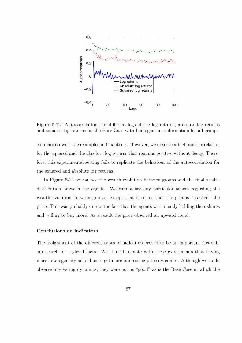
0 20 40 60 80 100−0.4
−0.2
0
0.2
0.4
0.6
Lags
Aut
ocor
rela
tions
Log returnsAbsolute log returnsSquared log returns
Figure 5-12: Autocorrelations for different lags of the log returns, absolute log returnsand squared log returns on the Base Case with homogeneous information for all groups.
comparison with the examples in Chapter 2. However, we observe a high autocorrelation
for the squared and the absolute log returns that remains positive without decay. There-
fore, this experimental setting fails to replicate the behaviour of the autocorrelation for
the squared and absolute log returns.
In Figure 5-13 we can see the wealth evolution between groups and the final wealth
distribution between the agents. We cannot see any particular aspect regarding the
wealth evolution between groups, except that it seems that the groups “tracked” the
price. This was probably due to the fact that the agents were mostly holding their shares
and willing to buy more. As a result the price observed an upward trend.
Conclusions on indicators
The assignment of the different types of indicators proved to be an important factor in
our search for stylized facts. We started to note with these experiments that having
more heterogeneity helped us to get more interesting price dynamics. Although we could
observe interesting dynamics, they were not as “good” as is the Base Case in which the
87
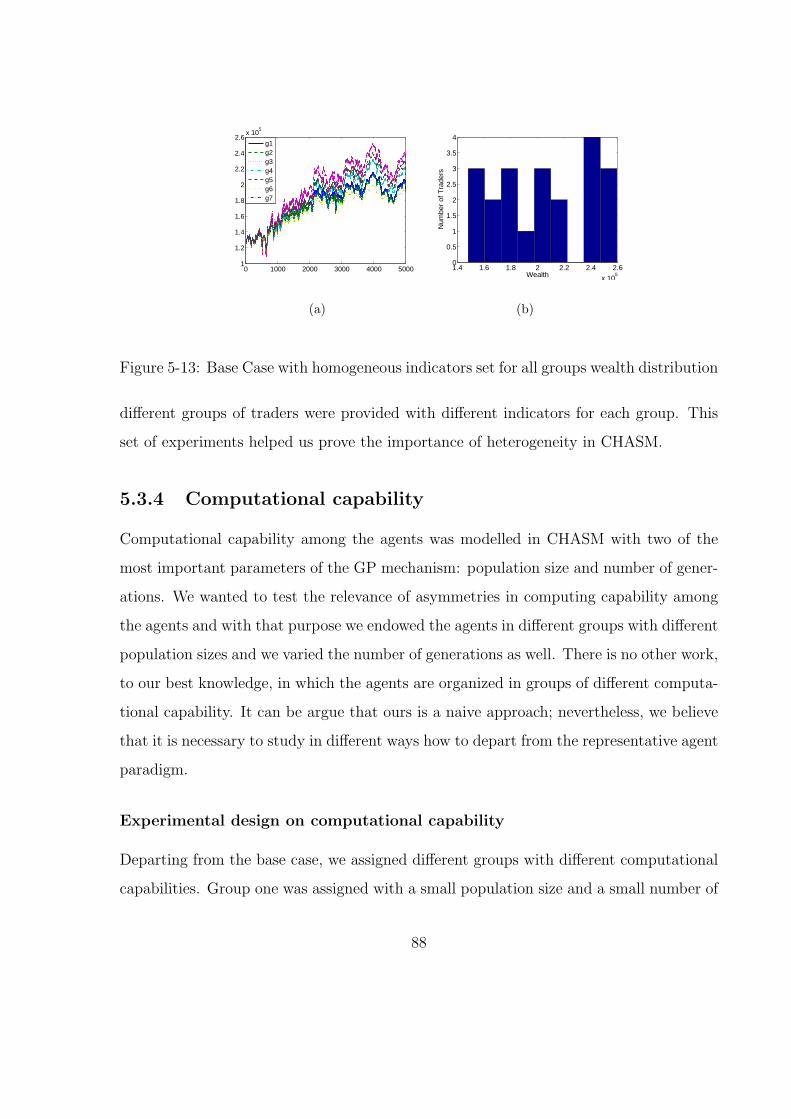
0 1000 2000 3000 4000 50001
1.2
1.4
1.6
1.8
2
2.2
2.4
2.6x 10
5
g1g2g3g4g5g6g7
(a)
1.4 1.6 1.8 2 2.2 2.4 2.6
x 105
0
0.5
1
1.5
2
2.5
3
3.5
4
Wealth
Num
ber
of T
rade
rs
(b)
Figure 5-13: Base Case with homogeneous indicators set for all groups wealth distribution
different groups of traders were provided with different indicators for each group. This
set of experiments helped us prove the importance of heterogeneity in CHASM.
5.3.4 Computational capability
Computational capability among the agents was modelled in CHASM with two of the
most important parameters of the GP mechanism: population size and number of gener-
ations. We wanted to test the relevance of asymmetries in computing capability among
the agents and with that purpose we endowed the agents in different groups with different
population sizes and we varied the number of generations as well. There is no other work,
to our best knowledge, in which the agents are organized in groups of different computa-
tional capability. It can be argue that ours is a naive approach; nevertheless, we believe
that it is necessary to study in different ways how to depart from the representative agent
paradigm.
Experimental design on computational capability
Departing from the base case, we assigned different groups with different computational
capabilities. Group one was assigned with a small population size and a small number of
88
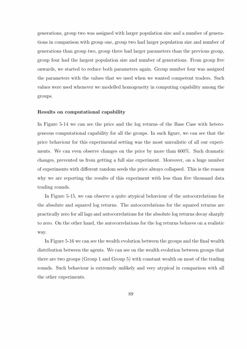
generations, group two was assigned with larger population size and a number of genera-
tions in comparison with group one, group two had larger population size and number of
generations than group two, group three had larger parameters than the previous group,
group four had the largest population size and number of generations. From group five
onwards, we started to reduce both parameters again. Group number four was assigned
the parameters with the values that we used when we wanted competent traders. Such
values were used whenever we modelled homogeneity in computing capability among the
groups.
Results on computational capability
In Figure 5-14 we can see the price and the log returns of the Base Case with hetero-
geneous computational capability for all the groups. In such figure, we can see that the
price behaviour for this experimental setting was the most unrealistic of all our experi-
ments. We can even observe changes on the price by more than 600%. Such dramatic
changes, prevented us from getting a full size experiment. Moreover, on a huge number
of experiments with different random seeds the price always collapsed. This is the reason
why we are reporting the results of this experiment with less than five thousand data
trading rounds.
In Figure 5-15, we can observe a quite atypical behaviour of the autocorrelations for
the absolute and squared log returns. The autocorrelations for the squared returns are
practically zero for all lags and autocorrelations for the absolute log returns decay sharply
to zero. On the other hand, the autocorrelations for the log returns behaves on a realistic
way.
In Figure 5-16 we can see the wealth evolution between the groups and the final wealth
distribution between the agents. We can see on the wealth evolution between groups that
there are two groups (Group 1 and Group 5) with constant wealth on most of the trading
rounds. Such behaviour is extremely unlikely and very atypical in comparison with all
the other experiments.
89
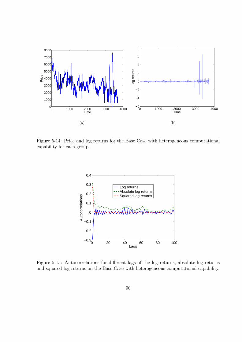
0 1000 2000 3000 40000
1000
2000
3000
4000
5000
6000
7000
8000
Time
Pric
e
(a)
0 1000 2000 3000 4000−6
−4
−2
0
2
4
6
8
Time
Log
retu
rns
(b)
Figure 5-14: Price and log returns for the Base Case with heterogeneous computationalcapability for each group.
0 20 40 60 80 100−0.3
−0.2
−0.1
0
0.1
0.2
0.3
0.4
Lags
Aut
ocor
rela
tions
Log returnsAbsolute log returnsSquared log returns
Figure 5-15: Autocorrelations for different lags of the log returns, absolute log returnsand squared log returns on the Base Case with heterogeneous computational capability.
90
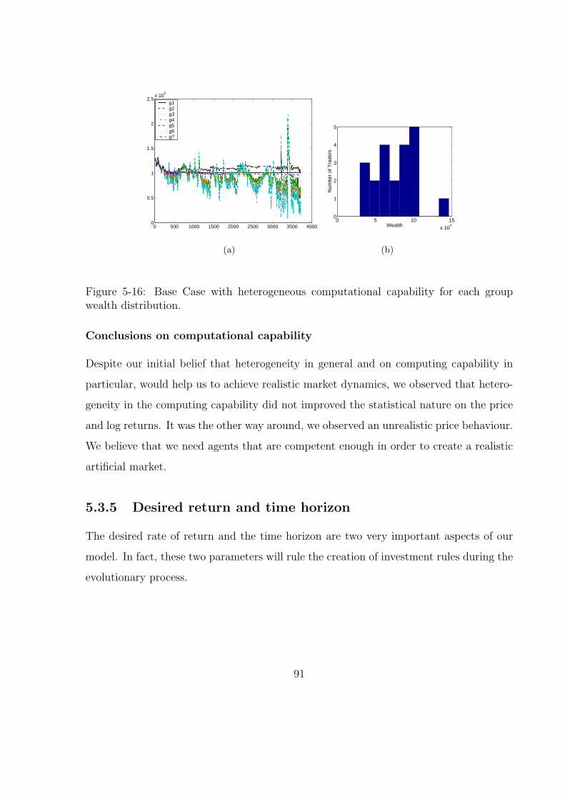
0 500 1000 1500 2000 2500 3000 3500 40000
0.5
1
1.5
2
2.5x 10
5
g1g2g3g4g5g6g7
(a)
0 5 10 15
x 104
0
1
2
3
4
5
Wealth
Num
ber
of T
rade
rs
(b)
Figure 5-16: Base Case with heterogeneous computational capability for each groupwealth distribution.
Conclusions on computational capability
Despite our initial belief that heterogeneity in general and on computing capability in
particular, would help us to achieve realistic market dynamics, we observed that hetero-
geneity in the computing capability did not improved the statistical nature on the price
and log returns. It was the other way around, we observed an unrealistic price behaviour.
We believe that we need agents that are competent enough in order to create a realistic
artificial market.
5.3.5 Desired return and time horizon
The desired rate of return and the time horizon are two very important aspects of our
model. In fact, these two parameters will rule the creation of investment rules during the
evolutionary process.
91

Experimental design on return and time horizon
In order to test the impact of such parameters on the behaviour of the price, we performed
several experiments in which we either had homogeneity among the different groups (like
in the Base Case) or we had heterogeneity in those two parameters. We have to stress
the importance of a careful selection of both parameters. For example, if for a particular
group, we programmed the traders in the group to ask for a large desired return on
their investment, then it was unreasonable to assign them a short time horizon. Such
unreasonable selection of both parameters could lead to unreasonable behaviour of the
agents, like agents that buy all the time or agents that do nothing the most of the time.
In other words, lets assume that we want to get a 20% return, clearly this is very difficult
to observe in real markets. However, if we want to achieve this in five days this is almost
impossible to observe. The result of such selection would generate training data in which
the class that would have the majority is the “Do Nothing” class 1
Results on return and time horizon
In Figure 5-17 we can see the price and the log returns of the Base Case with heteroge-
neous time horizon and expected return for all the groups. In such figure we can observe
an interesting price and the returns present volatility clustering. We will observe later in
this chapter the statistical properties of this experimental setting. Again, what we can
infer from this setting is that heterogeneity is very important to emulate the properties
of real prices.
In Figure 5-18, we can see that despite the somehow realistic behaviour of the auto-
correlations for the log returns, the autocorrelations for the absolute and squared returns
is highly positive and remains in such way for all the reported lags. We can say that
we would like to observe that the autocorrelations for the nonlinear functions of the log
returns to present higher decay.
1Remember that the agents are trying to classify each price point to belong to the classes: “Buy”,“Sell” and “Do Nothing”
92
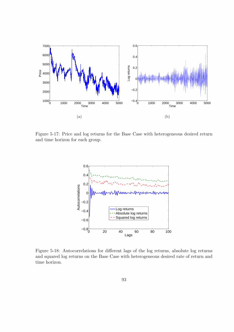
0 1000 2000 3000 4000 50001000
2000
3000
4000
5000
6000
7000
Time
Pric
e
(a)
0 1000 2000 3000 4000 5000−0.4
−0.2
0
0.2
0.4
0.6
Time
Log
retu
rns
(b)
Figure 5-17: Price and log returns for the Base Case with heterogeneous desired returnand time horizon for each group.
0 20 40 60 80 100−0.8
−0.6
−0.4
−0.2
0
0.2
0.4
0.6
Lags
Aut
ocor
rela
tions
Log returnsAbsolute log returnsSquared log returns
Figure 5-18: Autocorrelations for different lags of the log returns, absolute log returnsand squared log returns on the Base Case with heterogeneous desired rate of return andtime horizon.
93
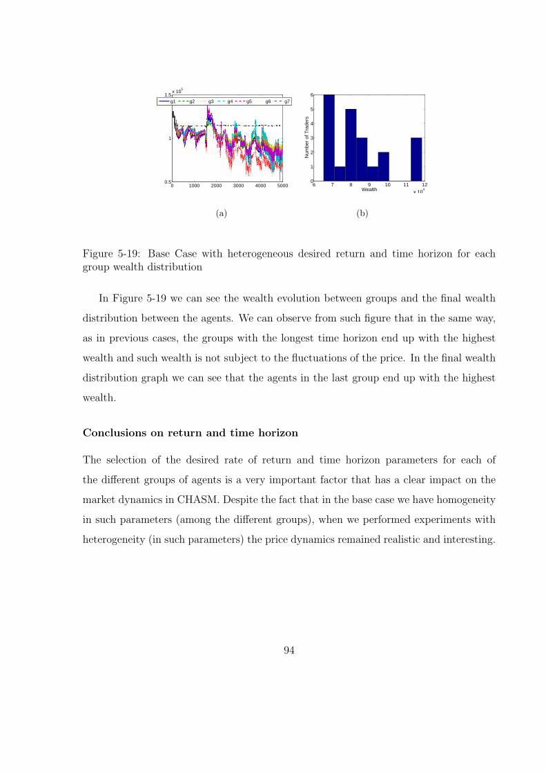
0 1000 2000 3000 4000 50000.5
1
1.5x 10
5
g1 g2 g3 g4 g5 g6 g7
(a)
6 7 8 9 10 11 12
x 104
0
1
2
3
4
5
6
Wealth
Num
ber
of T
rade
rs
(b)
Figure 5-19: Base Case with heterogeneous desired return and time horizon for eachgroup wealth distribution
In Figure 5-19 we can see the wealth evolution between groups and the final wealth
distribution between the agents. We can observe from such figure that in the same way,
as in previous cases, the groups with the longest time horizon end up with the highest
wealth and such wealth is not subject to the fluctuations of the price. In the final wealth
distribution graph we can see that the agents in the last group end up with the highest
wealth.
Conclusions on return and time horizon
The selection of the desired rate of return and time horizon parameters for each of
the different groups of agents is a very important factor that has a clear impact on the
market dynamics in CHASM. Despite the fact that in the base case we have homogeneity
in such parameters (among the different groups), when we performed experiments with
heterogeneity (in such parameters) the price dynamics remained realistic and interesting.
94
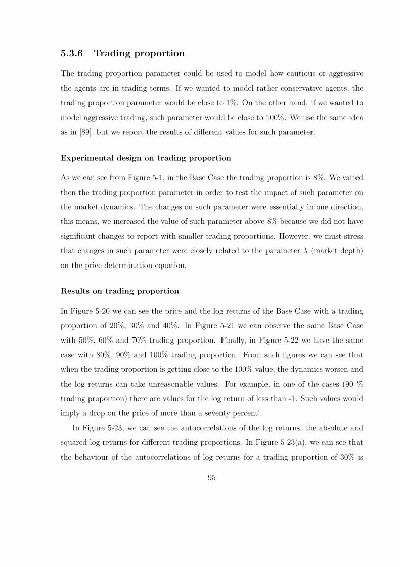
5.3.6 Trading proportion
The trading proportion parameter could be used to model how cautious or aggressive
the agents are in trading terms. If we wanted to model rather conservative agents, the
trading proportion parameter would be close to 1%. On the other hand, if we wanted to
model aggressive trading, such parameter would be close to 100%. We use the same idea
as in [89], but we report the results of different values for such parameter.
Experimental design on trading proportion
As we can see from Figure 5-1, in the Base Case the trading proportion is 8%. We varied
then the trading proportion parameter in order to test the impact of such parameter on
the market dynamics. The changes on such parameter were essentially in one direction,
this means, we increased the value of such parameter above 8% because we did not have
significant changes to report with smaller trading proportions. However, we must stress
that changes in such parameter were closely related to the parameter λ (market depth)
on the price determination equation.
Results on trading proportion
In Figure 5-20 we can see the price and the log returns of the Base Case with a trading
proportion of 20%, 30% and 40%. In Figure 5-21 we can observe the same Base Case
with 50%, 60% and 70% trading proportion. Finally, in Figure 5-22 we have the same
case with 80%, 90% and 100% trading proportion. From such figures we can see that
when the trading proportion is getting close to the 100% value, the dynamics worsen and
the log returns can take unreasonable values. For example, in one of the cases (90 %
trading proportion) there are values for the log return of less than -1. Such values would
imply a drop on the price of more than a seventy percent!
In Figure 5-23, we can see the autocorrelations of the log returns, the absolute and
squared log returns for different trading proportions. In Figure 5-23(a), we can see that
the behaviour of the autocorrelations of log returns for a trading proportion of 30% is
95
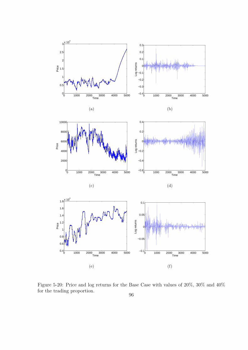
0 1000 2000 3000 4000 50000
0.5
1
1.5
2
2.5
3x 10
4
Time
Pric
e
(a)
0 1000 2000 3000 4000 5000−0.4
−0.3
−0.2
−0.1
0
0.1
0.2
0.3
Time
Log
retu
rns
(b)
0 1000 2000 3000 4000 50000
2000
4000
6000
8000
10000
Time
Pric
e
(c)
0 1000 2000 3000 4000 5000−0.6
−0.4
−0.2
0
0.2
0.4
Time
Log
retu
rns
(d)
0 1000 2000 3000 4000 50000.4
0.6
0.8
1
1.2
1.4
1.6
1.8x 10
4
Time
Pric
e
(e)
0 1000 2000 3000 4000 5000−0.1
−0.05
0
0.05
0.1
Time
Log
retu
rns
(f)
Figure 5-20: Price and log returns for the Base Case with values of 20%, 30% and 40%for the trading proportion.
96
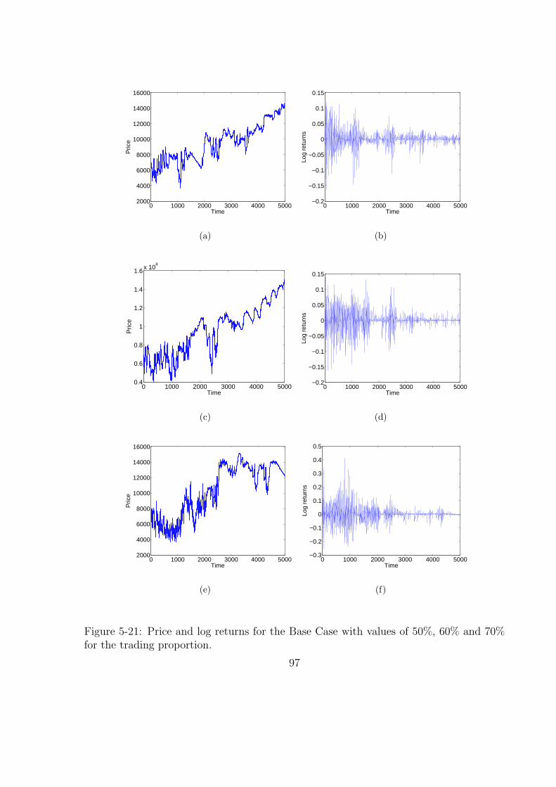
0 1000 2000 3000 4000 50002000
4000
6000
8000
10000
12000
14000
16000
Time
Pric
e
(a)
0 1000 2000 3000 4000 5000−0.2
−0.15
−0.1
−0.05
0
0.05
0.1
0.15
Time
Log
retu
rns
(b)
0 1000 2000 3000 4000 50000.4
0.6
0.8
1
1.2
1.4
1.6x 10
4
Time
Pric
e
(c)
0 1000 2000 3000 4000 5000−0.2
−0.15
−0.1
−0.05
0
0.05
0.1
0.15
Time
Log
retu
rns
(d)
0 1000 2000 3000 4000 50002000
4000
6000
8000
10000
12000
14000
16000
Time
Pric
e
(e)
0 1000 2000 3000 4000 5000−0.3
−0.2
−0.1
0
0.1
0.2
0.3
0.4
0.5
Time
Log
retu
rns
(f)
Figure 5-21: Price and log returns for the Base Case with values of 50%, 60% and 70%for the trading proportion.
97
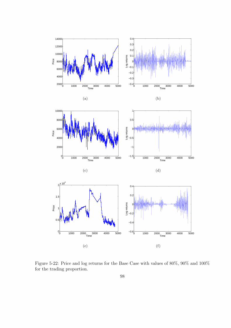
0 1000 2000 3000 4000 50002000
4000
6000
8000
10000
12000
14000
Time
Pric
e
(a)
0 1000 2000 3000 4000 5000−0.4
−0.3
−0.2
−0.1
0
0.1
0.2
0.3
0.4
Time
Log
retu
rns
(b)
0 1000 2000 3000 4000 50000
2000
4000
6000
8000
10000
Time
Pric
e
(c)
0 1000 2000 3000 4000 5000−1.5
−1
−0.5
0
0.5
1
Time
Log
retu
rns
(d)
0 1000 2000 3000 4000 50000
0.5
1
1.5
2x 10
4
Time
Pric
e
(e)
0 1000 2000 3000 4000 5000−0.6
−0.4
−0.2
0
0.2
0.4
Time
Log
retu
rns
(f)
Figure 5-22: Price and log returns for the Base Case with values of 80%, 90% and 100%for the trading proportion.
98
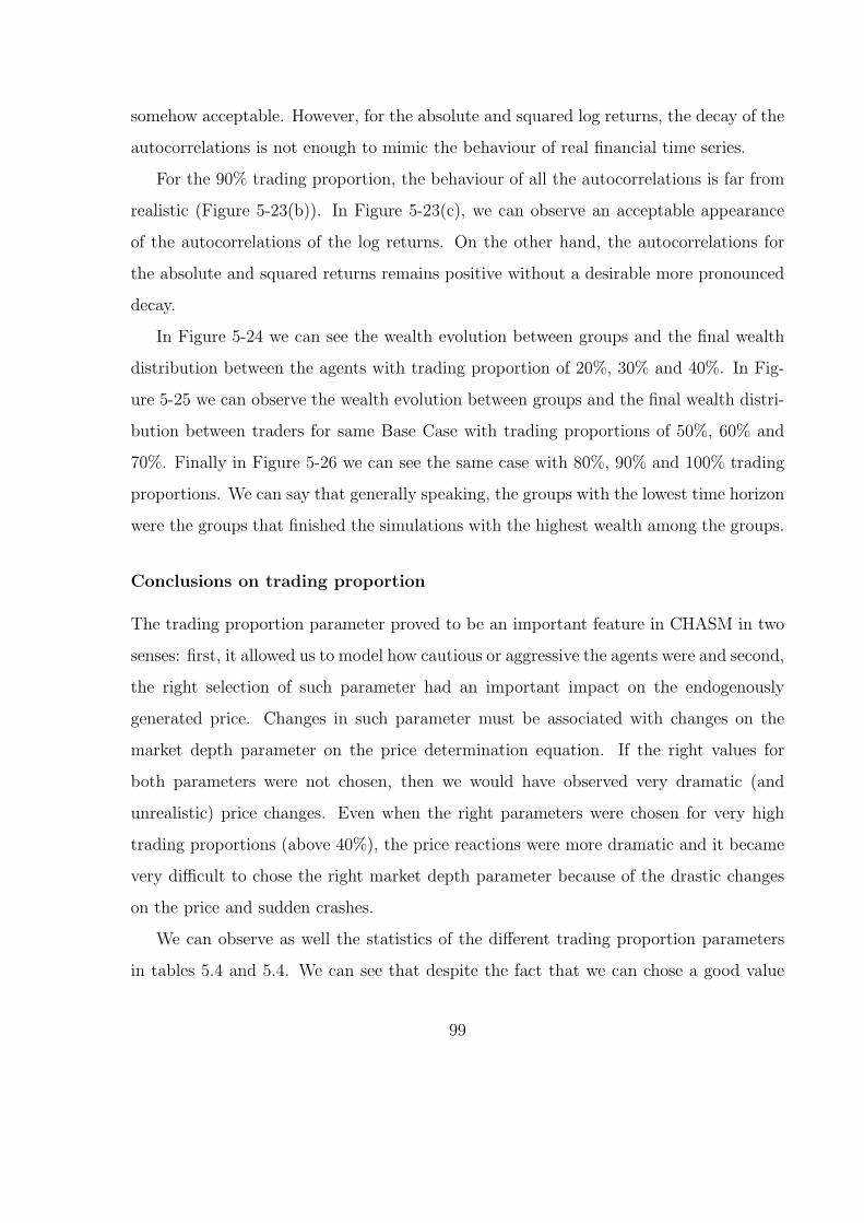
somehow acceptable. However, for the absolute and squared log returns, the decay of the
autocorrelations is not enough to mimic the behaviour of real financial time series.
For the 90% trading proportion, the behaviour of all the autocorrelations is far from
realistic (Figure 5-23(b)). In Figure 5-23(c), we can observe an acceptable appearance
of the autocorrelations of the log returns. On the other hand, the autocorrelations for
the absolute and squared returns remains positive without a desirable more pronounced
decay.
In Figure 5-24 we can see the wealth evolution between groups and the final wealth
distribution between the agents with trading proportion of 20%, 30% and 40%. In Fig-
ure 5-25 we can observe the wealth evolution between groups and the final wealth distri-
bution between traders for same Base Case with trading proportions of 50%, 60% and
70%. Finally in Figure 5-26 we can see the same case with 80%, 90% and 100% trading
proportions. We can say that generally speaking, the groups with the lowest time horizon
were the groups that finished the simulations with the highest wealth among the groups.
Conclusions on trading proportion
The trading proportion parameter proved to be an important feature in CHASM in two
senses: first, it allowed us to model how cautious or aggressive the agents were and second,
the right selection of such parameter had an important impact on the endogenously
generated price. Changes in such parameter must be associated with changes on the
market depth parameter on the price determination equation. If the right values for
both parameters were not chosen, then we would have observed very dramatic (and
unrealistic) price changes. Even when the right parameters were chosen for very high
trading proportions (above 40%), the price reactions were more dramatic and it became
very difficult to chose the right market depth parameter because of the drastic changes
on the price and sudden crashes.
We can observe as well the statistics of the different trading proportion parameters
in tables 5.4 and 5.4. We can see that despite the fact that we can chose a good value
99
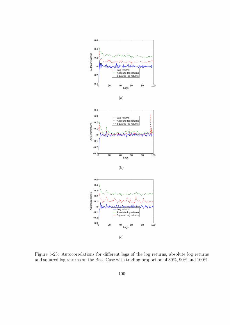
0 20 40 60 80 100−0.4
−0.2
0
0.2
0.4
0.6
LagsA
utoc
orre
latio
ns
Log returnsAbsolute log returnsSquared log returns
(a)
0 20 40 60 80 100−0.3
−0.2
−0.1
0
0.1
0.2
0.3
0.4
Lags
Aut
ocor
rela
tions
Log returnsAbsolute log returnsSquared log returns
(b)
0 20 40 60 80 100−0.3
−0.2
−0.1
0
0.1
0.2
0.3
0.4
0.5
Lags
Aut
ocor
rela
tions
Log returnsAbsolute log returnsSquared log returns
(c)
Figure 5-23: Autocorrelations for different lags of the log returns, absolute log returnsand squared log returns on the Base Case with trading proportion of 30%, 90% and 100%.
100
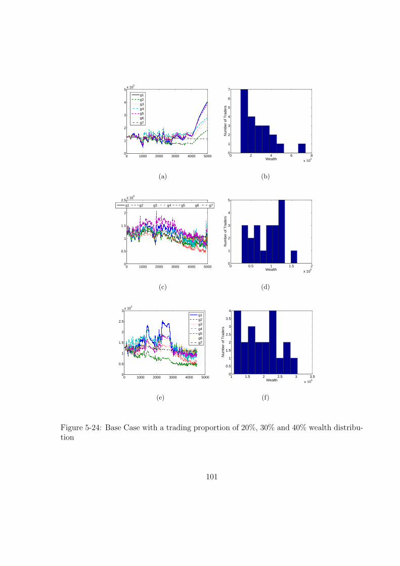
0 1000 2000 3000 4000 50000
1
2
3
4
5x 10
5
g1g2g3g4g5g6g7
(a)
0 2 4 6 8
x 105
0
1
2
3
4
5
6
7
Wealth
Num
ber
of T
rade
rs
(b)
0 1000 2000 3000 4000 50000
0.5
1
1.5
2
2.5x 10
5
g1 g2 g3 g4 g5 g6 g7
(c)
0 0.5 1 1.5 2
x 105
0
1
2
3
4
5
Wealth
Num
ber
of T
rade
rs
(d)
0 1000 2000 3000 4000 50000
0.5
1
1.5
2
2.5
3x 10
5
g1g2g3g4g5g6g7
(e)
1 1.5 2 2.5 3 3.5
x 105
0
0.5
1
1.5
2
2.5
3
3.5
4
Wealth
Num
ber
of T
rade
rs
(f)
Figure 5-24: Base Case with a trading proportion of 20%, 30% and 40% wealth distribu-tion
101
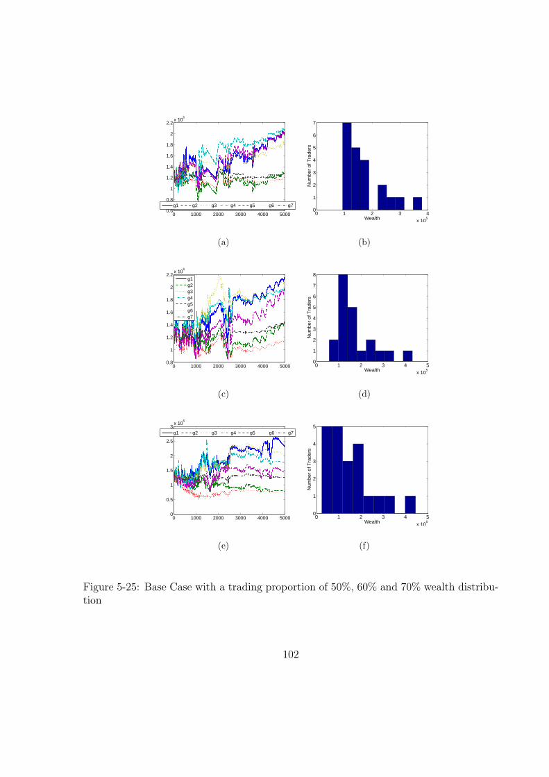
0 1000 2000 3000 4000 50000.6
0.8
1
1.2
1.4
1.6
1.8
2
2.2x 10
5
g1 g2 g3 g4 g5 g6 g7
(a)
0 1 2 3 4
x 105
0
1
2
3
4
5
6
7
Wealth
Num
ber
of T
rade
rs
(b)
0 1000 2000 3000 4000 50000.8
1
1.2
1.4
1.6
1.8
2
2.2x 10
5
g1g2g3g4g5g6g7
(c)
0 1 2 3 4 5
x 105
0
1
2
3
4
5
6
7
8
Wealth
Num
ber
of T
rade
rs
(d)
0 1000 2000 3000 4000 50000
0.5
1
1.5
2
2.5
3x 10
5
g1 g2 g3 g4 g5 g6 g7
(e)
0 1 2 3 4 5
x 105
0
1
2
3
4
5
Wealth
Num
ber
of T
rade
rs
(f)
Figure 5-25: Base Case with a trading proportion of 50%, 60% and 70% wealth distribu-tion
102
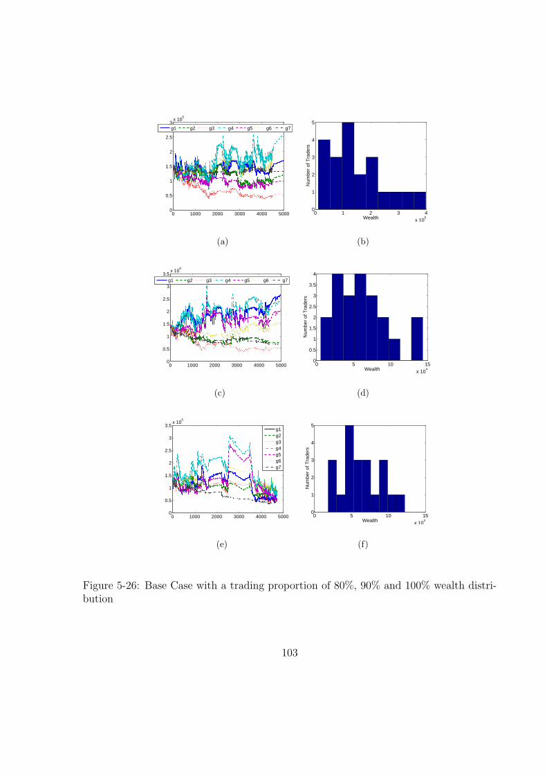
0 1000 2000 3000 4000 50000
0.5
1
1.5
2
2.5
3x 10
5
g1 g2 g3 g4 g5 g6 g7
(a)
0 1 2 3 4
x 105
0
1
2
3
4
5
Wealth
Num
ber
of T
rade
rs
(b)
0 1000 2000 3000 4000 50000
0.5
1
1.5
2
2.5
3
3.5x 10
5
g1 g2 g3 g4 g5 g6 g7
(c)
0 5 10 15
x 104
0
0.5
1
1.5
2
2.5
3
3.5
4
Wealth
Num
ber
of T
rade
rs
(d)
0 1000 2000 3000 4000 50000
0.5
1
1.5
2
2.5
3
3.5x 10
5
g1g2g3g4g5g6g7
(e)
0 5 10 15
x 104
0
1
2
3
4
5
Wealth
Num
ber
of T
rade
rs
(f)
Figure 5-26: Base Case with a trading proportion of 80%, 90% and 100% wealth distri-bution
103
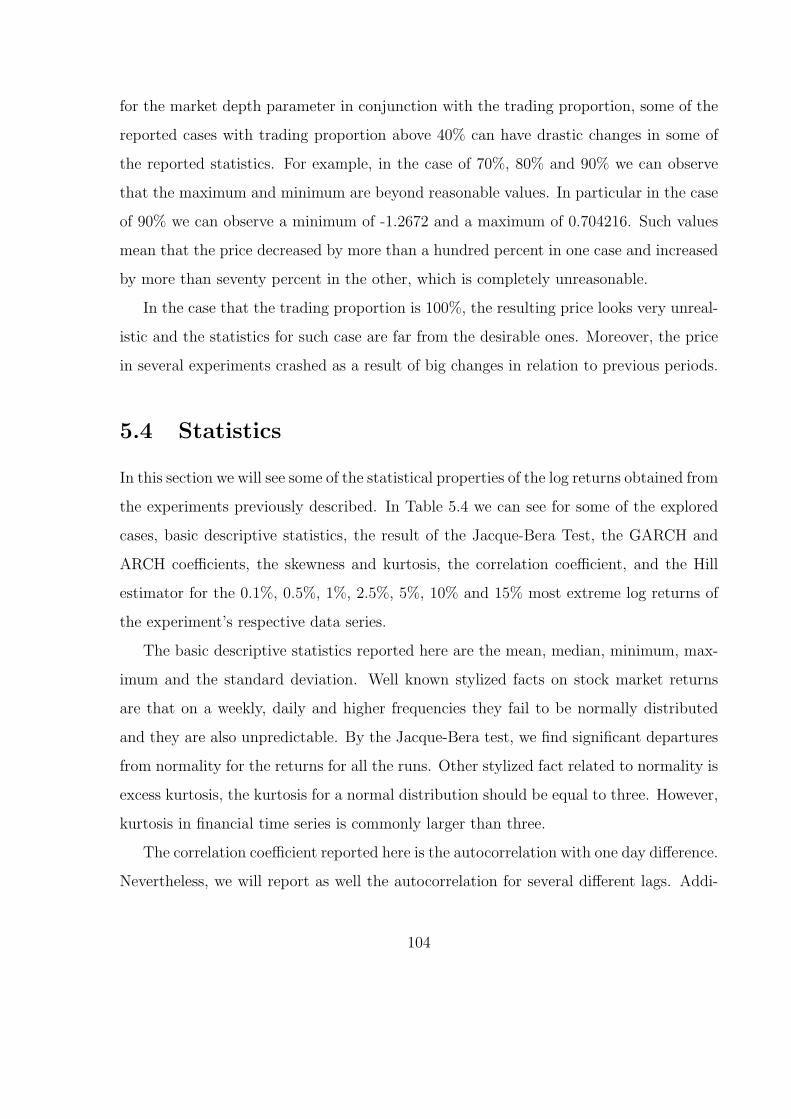
for the market depth parameter in conjunction with the trading proportion, some of the
reported cases with trading proportion above 40% can have drastic changes in some of
the reported statistics. For example, in the case of 70%, 80% and 90% we can observe
that the maximum and minimum are beyond reasonable values. In particular in the case
of 90% we can observe a minimum of -1.2672 and a maximum of 0.704216. Such values
mean that the price decreased by more than a hundred percent in one case and increased
by more than seventy percent in the other, which is completely unreasonable.
In the case that the trading proportion is 100%, the resulting price looks very unreal-
istic and the statistics for such case are far from the desirable ones. Moreover, the price
in several experiments crashed as a result of big changes in relation to previous periods.
5.4 Statistics
In this section we will see some of the statistical properties of the log returns obtained from
the experiments previously described. In Table 5.4 we can see for some of the explored
cases, basic descriptive statistics, the result of the Jacque-Bera Test, the GARCH and
ARCH coefficients, the skewness and kurtosis, the correlation coefficient, and the Hill
estimator for the 0.1%, 0.5%, 1%, 2.5%, 5%, 10% and 15% most extreme log returns of
the experiment’s respective data series.
The basic descriptive statistics reported here are the mean, median, minimum, max-
imum and the standard deviation. Well known stylized facts on stock market returns
are that on a weekly, daily and higher frequencies they fail to be normally distributed
and they are also unpredictable. By the Jacque-Bera test, we find significant departures
from normality for the returns for all the runs. Other stylized fact related to normality is
excess kurtosis, the kurtosis for a normal distribution should be equal to three. However,
kurtosis in financial time series is commonly larger than three.
The correlation coefficient reported here is the autocorrelation with one day difference.
Nevertheless, we will report as well the autocorrelation for several different lags. Addi-
104
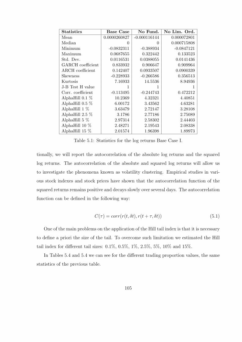
Statistics Base Case No Fund. No Lim. Ord.Mean 0.0000260827 -0.000116144 0.000072801Median 0 0 0.000715808Minimum -0.0832311 -0.388934 -0.0847121Maximum 0.0687655 0.322442 0.133523Std. Dev. 0.0116531 0.0388055 0.0141436GARCH coefficient 0.833932 0.906647 0.909964ARCH coefficient 0.142407 0.0933507 0.0900339Skewness -0.228933 -0.266586 0.356513Kurtosis 7.16933 14.5536 8.94936J-B Test H value 1 1 1Corr. coefficient -0.113495 -0.244743 0.472212AlphaHill 0.1 % 10.2369 4.32321 4.40851AlphaHill 0.5 % 6.00172 3.43562 4.63281AlphaHill 1 % 3.63479 2.72147 3.28108AlphaHill 2.5 % 3.1786 2.77186 2.75089AlphaHill 5 % 2.97314 2.58302 2.44403AlphaHill 10 % 2.48271 2.19543 2.08338AlphaHill 15 % 2.01574 1.96398 1.89973
Table 5.1: Statistics for the log returns Base Case I.
tionally, we will report the autocorrelation of the absolute log returns and the squared
log returns. The autocorrelation of the absolute and squared log returns will allow us
to investigate the phenomena known as volatility clustering. Empirical studies in vari-
ous stock indexes and stock prices have shown that the autocorrelation function of the
squared returns remains positive and decays slowly over several days. The autocorrelation
function can be defined in the following way:
C(τ) = corr(r(t, δt), r(t + τ, δt)) (5.1)
One of the main problems on the application of the Hill tail index is that it is necessary
to define a priori the size of the tail. To overcome such limitation we estimated the Hill
tail index for different tail sizes: 0.1%, 0.5%, 1%, 2.5%, 5%, 10% and 15%.
In Tables 5.4 and 5.4 we can see for the different trading proportion values, the same
statistics of the previous table.
105
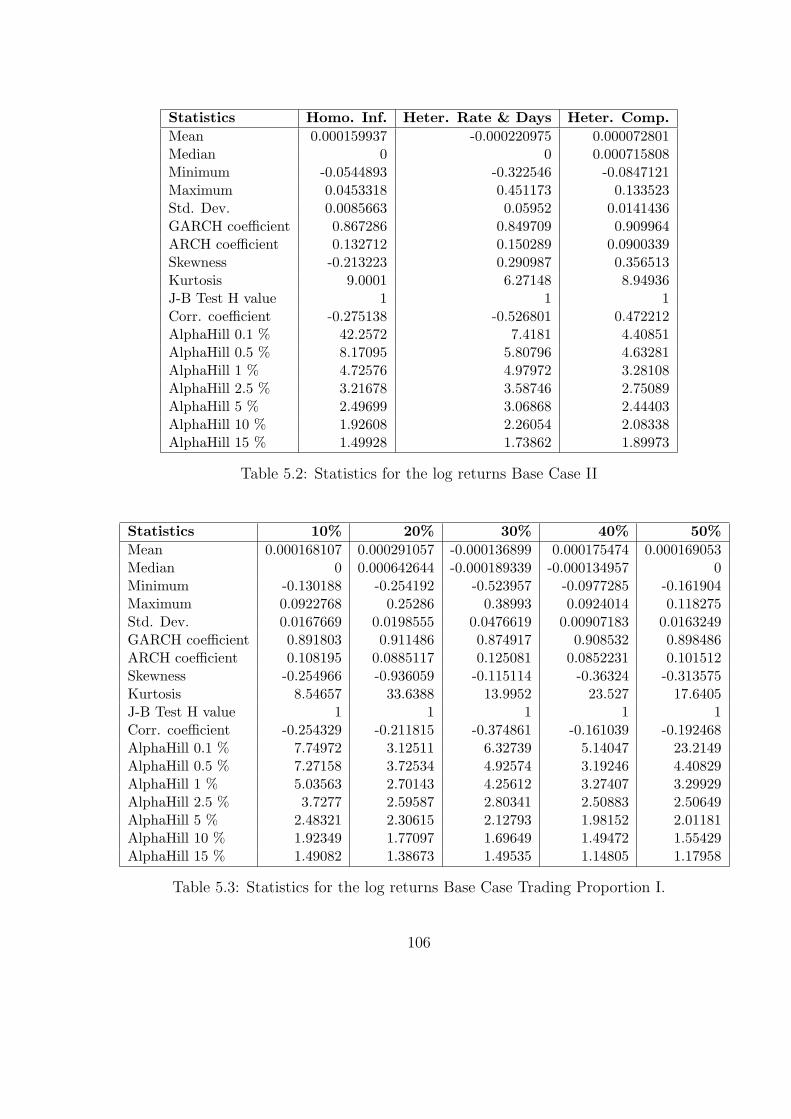
Statistics Homo. Inf. Heter. Rate & Days Heter. Comp.Mean 0.000159937 -0.000220975 0.000072801Median 0 0 0.000715808Minimum -0.0544893 -0.322546 -0.0847121Maximum 0.0453318 0.451173 0.133523Std. Dev. 0.0085663 0.05952 0.0141436GARCH coefficient 0.867286 0.849709 0.909964ARCH coefficient 0.132712 0.150289 0.0900339Skewness -0.213223 0.290987 0.356513Kurtosis 9.0001 6.27148 8.94936J-B Test H value 1 1 1Corr. coefficient -0.275138 -0.526801 0.472212AlphaHill 0.1 % 42.2572 7.4181 4.40851AlphaHill 0.5 % 8.17095 5.80796 4.63281AlphaHill 1 % 4.72576 4.97972 3.28108AlphaHill 2.5 % 3.21678 3.58746 2.75089AlphaHill 5 % 2.49699 3.06868 2.44403AlphaHill 10 % 1.92608 2.26054 2.08338AlphaHill 15 % 1.49928 1.73862 1.89973
Table 5.2: Statistics for the log returns Base Case II
Statistics 10% 20% 30% 40% 50%Mean 0.000168107 0.000291057 -0.000136899 0.000175474 0.000169053Median 0 0.000642644 -0.000189339 -0.000134957 0Minimum -0.130188 -0.254192 -0.523957 -0.0977285 -0.161904Maximum 0.0922768 0.25286 0.38993 0.0924014 0.118275Std. Dev. 0.0167669 0.0198555 0.0476619 0.00907183 0.0163249GARCH coefficient 0.891803 0.911486 0.874917 0.908532 0.898486ARCH coefficient 0.108195 0.0885117 0.125081 0.0852231 0.101512Skewness -0.254966 -0.936059 -0.115114 -0.36324 -0.313575Kurtosis 8.54657 33.6388 13.9952 23.527 17.6405J-B Test H value 1 1 1 1 1Corr. coefficient -0.254329 -0.211815 -0.374861 -0.161039 -0.192468AlphaHill 0.1 % 7.74972 3.12511 6.32739 5.14047 23.2149AlphaHill 0.5 % 7.27158 3.72534 4.92574 3.19246 4.40829AlphaHill 1 % 5.03563 2.70143 4.25612 3.27407 3.29929AlphaHill 2.5 % 3.7277 2.59587 2.80341 2.50883 2.50649AlphaHill 5 % 2.48321 2.30615 2.12793 1.98152 2.01181AlphaHill 10 % 1.92349 1.77097 1.69649 1.49472 1.55429AlphaHill 15 % 1.49082 1.38673 1.49535 1.14805 1.17958
Table 5.3: Statistics for the log returns Base Case Trading Proportion I.
106
Statistics 60% 70% 80% 90% 100%Mean 0.00017462 0.000133192 0.000132636 -0.000102296 -0.000178743Median -0.000324696 0 0 -0.000952448 -0.000405151Minimum -0.161402 -0.257609 -0.312498 -1.2672 -0.42604Maximum 0.140165 0.412267 0.302572 0.704216 0.357911Std. Dev. 0.0207563 0.0350901 0.0492769 0.0822619 0.0462254GARCH coefficient 0.854014 0.867212 0.957689 0.624627 0.955915ARCH coefficient 0.145984 0.132786 0.0423091 0.315992 0.0440828Skewness -0.272259 0.74249 0.00458005 -0.912754 -0.159393Kurtosis 11.4512 18.9064 8.01334 26.6752 14.3583J-B Test H value 1 1 1 1 1Corr. coefficient -0.274244 -0.304991 -0.253525 -0.251376 -0.233028AlphaHill 0.1 % 8.64128 5.45065 16.6104 5.82751 11.2171AlphaHill 0.5 % 5.51174 2.93004 4.62763 4.06839 4.00578AlphaHill 1 % 5.4529 3.3357 4.14005 3.90861 4.0789AlphaHill 2.5 % 3.19741 2.37363 3.22629 3.1404 2.78479AlphaHill 5 % 2.51586 2.21524 2.69543 2.73194 2.24749AlphaHill 10 % 1.45281 1.54832 2.0543 1.92623 1.54339AlphaHill 15 % 0.975017 1.09297 1.60132 1.52477 1.21649
Table 5.4: Statistics for the log returns Base Case Trading Proportion II.
5.5 Concluding Summary
In this chapter we described the investigated conditions under which some of the statis-
tical properties of the endogenously generated price resembles those of the real financial
markets. In CHASM we have the possibility of changing several parameters and changing
some of the important features of the model. A systematic experimental investigation
of changes in such parameters and characteristics was necessary. In this chapter we re-
ported the results of such experiments from which we can extract the following main
conclusions:
• The generation of limit orders proved to be an important factor to obtain realistic
price dynamics. Such limit orders were incorporated as part of a more complete
investment strategy of the agents
• The inclusion of the fundamental behaviour in one of the groups of agents was
an important factor to obtain a realistic price. We must stress that even when
107

just one of the groups has activated such behaviour, the obtained price improves
dramatically in terms of the desirable properties that we were looking for.
• The indicators and the heterogeneity on their assignment to the different groups of
agents is an important factor in our aim to obtain stylized facts. The assignment
of such indicators allowed us to model asymmetries on the information used by the
agents.
• Heterogeneity in the computational capability assigned to the groups of agents
proved to be of no utility or even harmful in our aim to get realistic price dynamics.
We attribute this to the fact that the sort of investment rules generated by stupid
agents are far from realistic and as consequence, the behaviour of such agents is
unrealistic as well.
• The desired rate of return and time horizon parameters, proved a key factor first
to generate realistic investment rules within the agent’s minds and second the
heterogeneity on the assignment of such parameters favoured the behaviour of the
endogenously generated price.
• The trading proportion parameter can be considered as a parameter that possesses
an important impact on the resulting price. Nevertheless, we must stress that
changes in such parameter should be accompanied by reasonable changes on the
market depth parameter on the price determination equation.
Additionally, with the objective of making a clear distinction of which scenarios and
the reported experiments are the ones that approach the most to real prices, we will
present a resume in a tabular form. The criteria that we used for our experiments to
determine if a price is or not (in our opinion) realistic are the following ones:
C1) GARCH and ARCH coefficients. Both coefficients and their addition must be less
than one.
108

C2) Kurtosis. The kurtosis of the price generated on the reported experiment should
be larger than three, which is the kurtosis of a normal distribution.
C3) Jacque-Bera Test H value. It is also necessary that the hypothesis that the gener-
ated price is drawn from a normal distribution is rejected.
C4) Alpha Hill estimator. It is required that the Hill estimator is between five and two
for different tail sizes.
C5) Autocorrelation I. The autocorrelation of the logarithmic returns should be around
zero, even for different lags.
C6) Autocorrelation II. A positive autocorrelation for lags close to zero and autocor-
relation decay for larger lags should be observed for the absolute and squared
logarithmic returns.
C7) Atypical behaviour. The prices generated under the evaluated scenario must not
show cyclical or another forms of atypical behaviour like huge changes or mono-
tonicity.
In Table 5.5 we report if the experiment passes or not each individual criterion. In
such table, on each row we report the analysis for a price generated under one of the
scenarios described on this chapter and each column represents one of the criterion. We
can see that the two most successful experiments are: the one in which we provided the
groups with different time horizon and expected return, and the one in which we used a
trading proportion of 30%. Interestingly, the criteria number six seems to be the most
difficult to satisfy and none of our experiments was able to reproduce such property.
109
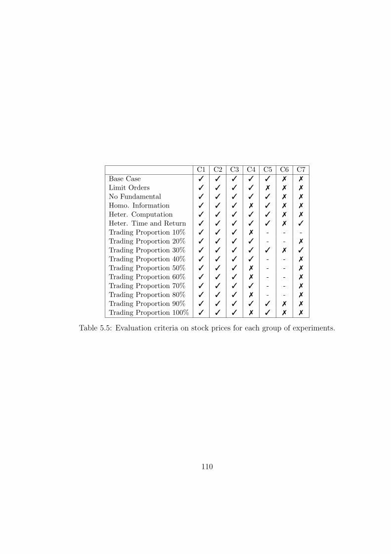
C1 C2 C3 C4 C5 C6 C7Base Case 3 3 3 3 3 7 7
Limit Orders 3 3 3 3 7 7 7
No Fundamental 3 3 3 3 3 7 7
Homo. Information 3 3 3 7 3 7 7
Heter. Computation 3 3 3 3 3 7 7
Heter. Time and Return 3 3 3 3 3 7 3
Trading Proportion 10% 3 3 3 7 - - -Trading Proportion 20% 3 3 3 3 - - 7
Trading Proportion 30% 3 3 3 3 3 7 3
Trading Proportion 40% 3 3 3 3 - - 7
Trading Proportion 50% 3 3 3 7 - - 7
Trading Proportion 60% 3 3 3 7 - - 7
Trading Proportion 70% 3 3 3 3 - - 7
Trading Proportion 80% 3 3 3 7 - - 7
Trading Proportion 90% 3 3 3 3 3 7 7
Trading Proportion 100% 3 3 3 7 3 7 7
Table 5.5: Evaluation criteria on stock prices for each group of experiments.
110

Chapter 6
Co-evolution in CHASM
Co-evolution is said to take place when two or more lineages have an impact on each
other’s selection mechanism and cause changes on each other that increases fitness. This
mutual adaptation happens whenever certain ecological interaction derives into fitness
effects for all the participants.
Co-evolution in Evolutionary Computation and in particular in GP, is an important
area of study in Computer Science and has been used in the modelling of independent
agents in the past [114]. Moreover, the notion of evolving competitively populations and
in particular decision trees has been intensively studied in [7], [108] and [176].
We aim to model traders in real markets. Therefore, we consider co-evolution to be of
central importance in our work, because in real life the traders certainly have an influence
in each other’s trading strategies. Additionally, it is common for them to change their
strategy if they are not performing well in relation to the other market participants.
Therefore, in our opinion it is necessary to include in our market model the co-evolution
of the agents’ trading strategies. In our market the co-evolution of such strategies will
be modelled by using two different mechanisms:
• The endogenous generation of the risky asset’s price.
• The regeneration of the technical trader’s “strategies”. In CHASM, this can be
111
done in a fixed or endogenous way.
In our market, the population of investment rules of each trader co-evolves through
the price. The effectiveness of each rule (its forecasting precision) determines the prob-
ability of it being selected to be part of the population of the next generation during
the evolutionary process. The precision of a certain rule belonging to a particular trader
depends on the rules of the other traders because they will have to change his rules if
their performance on the market is not good. Therefore, it affects the trader’s fitness.
Our work differs from [53] in the sense that each of our agents runs a GP mechanism
“inside their minds” and possess a population of rules (trees)1. Another important dif-
ference with the previously cited work and some others, is that we do not model social
learning or explicit interactions between the agents. The interaction between the agents
is modelled solely through the price.
In [211] the authors acknowledge the necessity of having to model the individual
intelligence of the agents. Clearly, their approach of previous works[53] was not sufficient
to achieve realistic modelling of certain aspects of the market participants. However,
they recognize the complexity of such task and the intensive computation involved on
the simulation of such market. Our work is much more computationally demanding than
the model proposed in [53]. Nevertheless, we are able to model complex traders with a
realistic formation process of investment rules.
Regarding the learning process, in CHASM the user can model the agents, so that
they are able to adapt to the new conditions of the market, either periodically (with
a user defined periodicity) or with a periodicity that is endogenously generated by a
behavioural constraint known as the Red Queen constraint. CHASM allows those two
different conditions to trigger learning because we want to contrast both ways, although
we believe that learning in an endogenous way is more realistic. Besides, we believe
that the statistical properties of stock returns will emerge from the activation of the Red
1In [53] there are basically two GP mechanisms, one is the main mechanism which possess thepopulations of traders and the other GP mechanism is known as the “Business School”
112
Queen constraint.
Adaptation of the market participants with fixed periodicity has been used on previous
works, eg. [16]. However, we consider it unrealistic because in real life, the traders do
not change their investment strategies (at least not the totality) in strictly fixed way.
Moreover, the findings reported in [124] are very revealing about the importance of the
learning periodicity. In [124] the authors reported the differences on the price properties
due to changes on the frequency of the retraining procedure and the memory length of
the agents.
The condition to trigger endogenously the learning process has been modelled in
previous works. For example, the notion of self realization was modelled in [53] and
[211], which is based on a notion of rank. However, we believe that such approach is not
a hundred percent realistic. We believe that the traders’ decision to change their strategy
must be motivated by their performance on the market in terms of wealth. It is very
likely that this decision is strongly related to the other market participants’ performance.
This was recognized as an important aspect in Artificial Financial Markets in [118] by
LeBaron:
“This suggests an approach which looks at performance which can only be
fully evaluated relative to others in the market. Agent based markets provide
a perfect setting for testing these ideas, but this opens the question of how
and where to implement evolution”
To summarize, we believe that the modelling of co-evolution in simulated markets
is important. Therefore, we make it a key feature in CHASM. It is possible to model
the way in which learning is triggered in two different ways: with fixed periodicity or
endogenously. In CHASM we are able to model such forms of adaptation and we will
report the results of some experiments later in this chapter.
113
6.1 Social learning and herd behaviour
In this section we will discuss some of the different possibilities to model the interactions
among the agents and the way in which they update their belief systems.
In the Artificial Markets literature, there are different means to model the interaction
among the agents and their adaptation or learning. In some works, we can find that the
interaction between the agents has been modelled explicitly, eg. see [137], [141], [60], [81].
Alternatively, it could be implicit on the price, as in our case. In terms of adaptation and
learning, there is a wide range of possibilities. We can find among such possibilities from
agents with zero intelligence [91], [184], to many different machine learning mechanisms
like neural networks [208], bayesian learning, genetic algorithms [16], learning classifier
systems [170], genetic programming [53], [149], [153], [152], etc.
6.1.1 Individual versus Social Learning
In the case that an Evolutionary Computation technique is being used to model the
agents’ learning process, there are two main possibilities for such modelling: Single Pop-
ulation (SP) or Multiple Population (MP).
When SP is used, each individual of the population represents an economic agent.
This means that there is just one evolutionary mechanism driving the simulation and
the agents have no control over it. On the other hand, in the case of MP each agent
possesses a population of individuals and “runs” an evolutionary mechanism by herself.
There are advantages and disadvantages when using either of the two approaches.
Nevertheless, we can point out to the ones that we believe are the most significant:
when a SP evolutionary process is being used, the individual intelligence is not being
explicitly modelled, when a MP evolutionary process is being used, social learning must
be represented in an explicit way.
In [53] and in a later and extended work [211] the authors explore two different archi-
tectures of an Artificial Stock Market. In the first one, they propose basically a SP-GP
114
mechanism enhanced with another SP-GP mechanism known as the “Business School”.
In the second one, the authors propose a MP-GP mechanism for the agents and in ad-
dition they preserve the “Business School” as well. However, due to the computational
demand of the simulation, the extension in the second work could not be taken further
because the agents have very limited “intelligence”, as the population size of the GP
mechanism of each agent is rather small. In our case, we found in our experiments that
having limited computing capability in the traders’ GP mechanism implies that we would
have prices with non desirable properties.
In the Santa Fe’s experiments, they use a MP-GA and the change of behaviour is
exogenously imposed by the experimenters [16]. Chen and Yeh proposed an endogenous
scheme for retraining in [53]. In their experiments, prices in the artificial market are
determined by artificial agents, which were modelled by genetic programs. They studied
when and by how much agents (which were investors) retrained themselves. From the
experimenters’ point of view, retraining was endogenously motivated by ‘peer pressure’
and self-realization. They prescribed a way in which agents looked for ‘better’ invest-
ment rules. To make an analogy to real world phenomena, they called this procedure
’Visiting the Business School’. Driven by differences in performance (as opposed to being
determined by experimental parameters), agents co-evolve.
Our approach is similar to the architecture in [211] in the sense that each of the
agents runs a GP mechanism. However, in our market there is no “Business School” or
any other explicit mechanism of social interaction. In our case, the interaction through
the price is enough to replicate some of the stylized facts. Besides, we believe that the
inclusion of “trend following” indicators as part of the agents information, can replace an
explicit model of interaction among them. Moreover, as it was stated at the beginning
of this work, the modelling or implications of social interactions in financial markets is
beyond the scope of our research.
115
6.1.2 Herd behaviour
It is now accepted that some fluctuations of stock prices are not explained by the arrival
of information or changes in fundamentals. In the recent years, it has been recognized
the impact that some social phenomena have on the prices of the financial assets. Among
them we find the so called “Herd behaviour”. A good introduction to this concept in
finance is [33], which is a review of the theoretical and empirical research on the field.
Herd behaviour is said to happen when a group of individuals act in the same way
without the existence of an explicit coordination mechanism. Such tendency to act in a
similar way suggests certain irrationality, in particular in financial markets. In [173] the
author describes two different approaches to model such phenomenon like the “Informa-
tional Cascades” in [26] and [32]. In such models, people acquire information in sequence
by observing the actions of other preceding individuals in the group. The individuals that
come after may ignore their own information and decide that the information revealed
by their predecessors is more valuable.
Another approach to the study of herd behaviour is to analyze the transmission of
information within groups of individuals by means of “conversation analysis” [92] or
“socio-cognition” [127]. This approach follows the premise that the human society has
had an evolutionary advantage in acting as a unit and human communication should be
acknowledged as part of the success in the competition with other species. Nevertheless,
it seems that sometimes such collective behaviour could be harmful or even counterpro-
ductive and the occurrence of bubbles and crashes in financial markets is an illustrative
example.
There exists some empirical evidence of herd behaviour in financial markets as it has
been documented in the case of mutual funds in [94] and in the case of security analysts
in [202]. Therefore, it is natural to use Artificial Financial Markets to investigate some of
the implications of such phenomenon in finance. Herding is explicitly modelled in some
important works like [137], [141], [60].
In [137], Lux models explicitly the factors which influence the behaviour of some
116
traders in his model. In [60], Cont and Bouchaud established a relation between the Fat
Tails of the returns and herding in financial markets. In [141], Lux and Marchesi modelled
different types of agents (fundamental and noise traders) with changes of behaviour
between them and herding taking place among the noise traders.
Despite the importance of this topic in finance we did not modelled in an explicit way
the interaction among traders. We left it for the technical analysis to summarize much
of the collective behaviour and the inclusion of some trend following and momentum
indicators allowed us to implicitly model social interaction.
6.2 The Red Queen principle in evolution and eco-
nomics
In our research we have a market populated by a co-evolving population of agents, each
attempting to enhance its fitness relative to others. This is inspired by the Red Queen
principle, based on the observation made to Alice by the Red Queen in Lewis Caroll’s
Through the Looking Glass: “in this place it takes all the running you can do, to keep in
the same place”.
The Red Queen principle was originally proposed by the evolutionary biologist Leigh
van Valen in [200] as a metaphor of a co-evolutionary arms race between species. In cases
in which the competition for scarce resources rules the behaviour of the participants; the
important performance measure is relative to the other individuals involved in such arms
race.
The Red Queen principle has been studied in Computer Science, more specifically
in competitive co-evolution [163], [160]. In particular, in [58] the authors propose some
means to measure the progress in computer simulated co-evolution. The Red Queen effect
has been also studied in the context of Economics in the past. In [167], the author claims
that the evolution of intelligence itself is hypothesized to arise as a Red Queen type arms
race giving rise to Machiavellian behaviour in social interactions. In [168] the author
117

describes the relation between the evolution of complex organisms, the reasons behind
sexual reproduction, the emergence of high intelligence and the Red Queen effect. In [147]
there is a fuller discussion of the relevance of the Red Queen principle in Economics.
In competitive co-evolution, the Red Queen principle, therefore, entails constraints on
performance enhancement of all individuals, if each is to maintain status quo in relative
fitness measured by an index relating to aggregate performance. However, such arms
race could lead in some occasions to a decrease in fitness in absolute terms. When this
phenomena is present in an evolutionary system, it is said that such system presents
the Red Queen Dynamics. Moreover, in some specific problems the use of competitive
co-evolution might be less effective than other techniques as it was shown in [163].
6.2.1 The Red Queen in CHASM
The model presented in this work recurs to the Red Queen principle to reproduce the
interaction and the co-evolution of the market agents. We consider that the need for
adaptation to the new conditions of the environment must be modelled explicitly and
should be done in an endogenous way.
One of the main criticisms to the agent-based modelling is the fact that such models
need a lot of calibration and their behaviour depends heavily on a certain number of
parameters. It is indeed difficult to justify some of the values that such parameters take.
To avoid this situation, we model endogenously the majority of the processes or at least
some of the most important ones.
In CHASM, the Red Queen principle will be modelled through the Red Queen Con-
straint. Such behavioural constraint will force a trader to search for new investment
rules whenever she is being “left behind”. More specifically, a trader will launch a GP
mechanism considering the most recent information (the most recent price history and
the relevant indicators) whenever her wealth is below the population’s average wealth.
As it was pointed out at the beginning of this chapter and as it was recognized in [118]
by LeBaron: “A trader’s performance depends critically on the behavior of others”.
118
In order to avoid the renovated trader to be completely unrelated with the trader that
entered into this retraining phase; the renovated trader will inherit half of her initial pop-
ulation from the original trader. Such decision has two objectives in mind: first, allowing
the evolutionary process to start from scratch is equivalent to inserting a completely new
trader into the population of agents. Second, there is already a certain knowledge on the
traders’ population of rules, the recombination with new ideas should allow the agent to
improve without discarding all the experience gained during the previous trading rounds.
6.2.2 Experimental design
To experimentally test the impact of the Red Queen principle, we designed a set of
experiments in which the agents will retrain in a fixed or endogenous way. Then, we
observe the differences in the statistical properties of the stock returns and the agents’
wealth distribution.
In such experiments we defined some study cases which we considered to be interest-
ing. This was taking into account the experience gained with the experiments described
in the previous chapter. Such study cases were different variations of the factors that we
identified as important in the previous phase of experimentation.
We first executed the simulation program with the parameters that we consider to
be appropriate to get realistic statistical behaviour of the log returns. Afterwards, we
observed the price behaviour and we performed a series of statistical tests to identify
if the price presented the stylized facts. In case the stylized facts were not replicated
we tried another parameter constellation and so on until we got the desired properties.
After getting the appropriate parameters, we executed the market with the same setting
but allowing the agents to learn with fixed periodicity. Then, we reported the statistics
of such execution. For the experiments reported in this chapter learning with fixed
periodicity was triggered every one thousand trading periods.
Using the same configuration of the two previous experiments (without learning and
learning with fixed periodicity), we allowed the agents to retrain in an endogenous way,
119
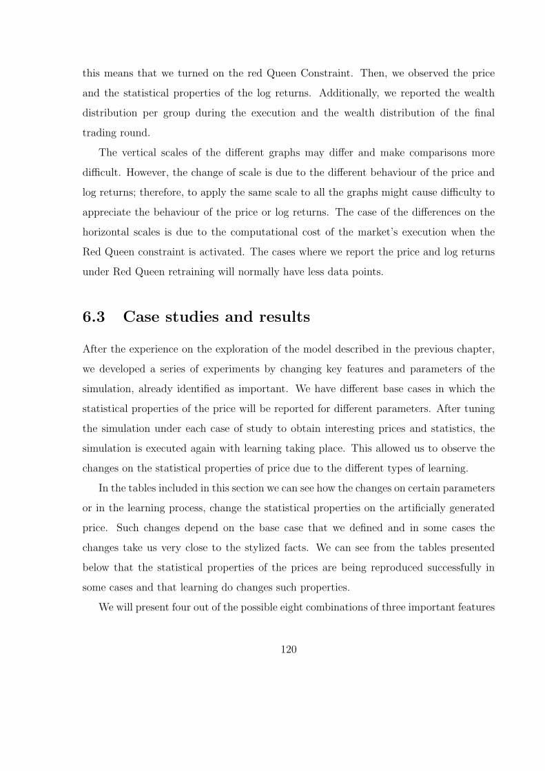
this means that we turned on the red Queen Constraint. Then, we observed the price
and the statistical properties of the log returns. Additionally, we reported the wealth
distribution per group during the execution and the wealth distribution of the final
trading round.
The vertical scales of the different graphs may differ and make comparisons more
difficult. However, the change of scale is due to the different behaviour of the price and
log returns; therefore, to apply the same scale to all the graphs might cause difficulty to
appreciate the behaviour of the price or log returns. The case of the differences on the
horizontal scales is due to the computational cost of the market’s execution when the
Red Queen constraint is activated. The cases where we report the price and log returns
under Red Queen retraining will normally have less data points.
6.3 Case studies and results
After the experience on the exploration of the model described in the previous chapter,
we developed a series of experiments by changing key features and parameters of the
simulation, already identified as important. We have different base cases in which the
statistical properties of the price will be reported for different parameters. After tuning
the simulation under each case of study to obtain interesting prices and statistics, the
simulation is executed again with learning taking place. This allowed us to observe the
changes on the statistical properties of price due to the different types of learning.
In the tables included in this section we can see how the changes on certain parameters
or in the learning process, change the statistical properties on the artificially generated
price. Such changes depend on the base case that we defined and in some cases the
changes take us very close to the stylized facts. We can see from the tables presented
below that the statistical properties of the prices are being reproduced successfully in
some cases and that learning do changes such properties.
We will present four out of the possible eight combinations of three important features
120
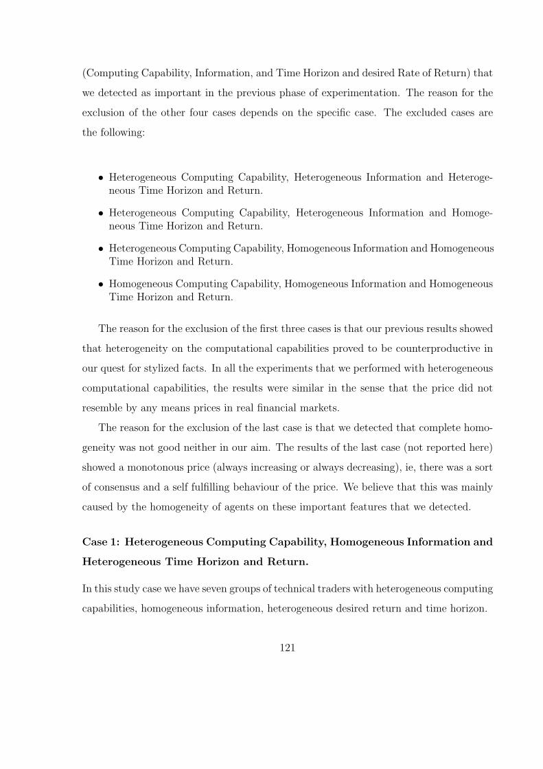
(Computing Capability, Information, and Time Horizon and desired Rate of Return) that
we detected as important in the previous phase of experimentation. The reason for the
exclusion of the other four cases depends on the specific case. The excluded cases are
the following:
• Heterogeneous Computing Capability, Heterogeneous Information and Heteroge-neous Time Horizon and Return.
• Heterogeneous Computing Capability, Heterogeneous Information and Homoge-neous Time Horizon and Return.
• Heterogeneous Computing Capability, Homogeneous Information and HomogeneousTime Horizon and Return.
• Homogeneous Computing Capability, Homogeneous Information and HomogeneousTime Horizon and Return.
The reason for the exclusion of the first three cases is that our previous results showed
that heterogeneity on the computational capabilities proved to be counterproductive in
our quest for stylized facts. In all the experiments that we performed with heterogeneous
computational capabilities, the results were similar in the sense that the price did not
resemble by any means prices in real financial markets.
The reason for the exclusion of the last case is that we detected that complete homo-
geneity was not good neither in our aim. The results of the last case (not reported here)
showed a monotonous price (always increasing or always decreasing), ie, there was a sort
of consensus and a self fulfilling behaviour of the price. We believe that this was mainly
caused by the homogeneity of agents on these important features that we detected.
Case 1: Heterogeneous Computing Capability, Homogeneous Information and
Heterogeneous Time Horizon and Return.
In this study case we have seven groups of technical traders with heterogeneous computing
capabilities, homogeneous information, heterogeneous desired return and time horizon.
121

The purpose of testing and analyzing this specific case was to verify the impact
that the asymmetry in computational capability (in terms of the GP mechanism) has in
the market. In other words, heterogeneity in computing capability refers to two of the
GP parameters assigned to the agents: population size and number of generations. We
identified these two parameters as the most relevant ones for measuring the computational
capabilities of the agents. In this experiment, the first group of agents was provided with
the smallest number of generations and population size, the second group had a bigger
number of generations and population size than the first group, the third had bigger
numbers in both parameters than the second group, the fourth was the most competent
of all the different groups and then we started to reduce the population size and number
of generations for the remaining three groups.
The obtained prices were the least successful to replicate the stylized facts in com-
parison with the other cases. We expected such results to a certain extent because it is
very important that the behaviour of the agents is closer to reality, we need competent
traders to participate in our market. Otherwise, the price and its statistical properties
do not resemble real data. We found very unrealistic behaviour of the price even with
learning taking place, in fact the price behaviour is worst when learning happens as we
can see in Figure 6-1.
Figures 6-1(a) and 6-1(b) show the price and log returns without learning taking place.
The next two figures 6-1(c) and 6-1(d) show the price and log returns when learning with
fixed periodicity takes place. Finally, the figures 6-1(e) and 6-1(f) show the price and
log returns when the Red Queen constraint is applied. In such figure, we can observe
that the price, when learning is not taking place, looks somehow realistic. However, if
we observe the other two cases (when learning takes place); then, it was clear that under
these conditions and parameter constellation we would not get any closer to the stylized
facts.
In Figures 6-1(c) and 6-1(e) we can appreciate the sort of things that can go wrong
in artificial financial markets research and why it is difficult to find the conditions under
122

which the simulated market resembles real markets. By looking at such figures we can
see that the agents’ perception about the price converged after a certain period and then
there was no trading activity anymore. In other words, there were no bids or offers and
the agents’ were essentially maintaining their current positions. The trading activity
stopped around the trading period 5000 in the case where learning was taking place in
a fixed way. In the case where learning was controlled by the Red Queen constraint, the
same thing happened much earlier (around the trading period 1250).
In Figure 6-2 we can observe the wealth evolution and the wealth distribution in
the final round for Case 1 in three different scenarios: without learning taking place,
(figures 6-2(a) and 6-2(d)); when learning with fixed periodicity is happening (figures
6-2(c) and 6-2(d)) and when the Red Queen Constraint is being activated (figures 6-2(e)
and 6-2(f)). In this figure is now clear that convergence takes place under this case of
study. We observed a convergence of the price in Figure 6-1 and we observe convergence
on wealth among the different traders when learning happens.
Figure 6-3 shows the autocorrelations for different lags of Case 1 (No learning, Fixed
learning and Learning with the Red Queen constraint). Regarding the autocorrelations
of the above mentioned three cases, we can see that the case where learning does not
take place is the more realistic. On the other hand, in the cases where learning takes
place we observe a very unrealistic behaviour of the autocorrelations for the log returns,
the absolute and the squared log returns.
Finally, Table 6.3 shows the statistics corresponding to the first case of study. In
addition to the standard descriptive statistics we are reporting the correlation, GARCH
and ARCH coefficients, skewness, kurtosis, the Hill estimator for different tail sizes and
the Jacque Bera test for normality. In such table we can see that the values reported are
not very well related to the stylized facts that we are looking for, despite that normality
is rejected. In particular the values for the Hill estimator for the fixed learning case are
well out of the desired range.
123
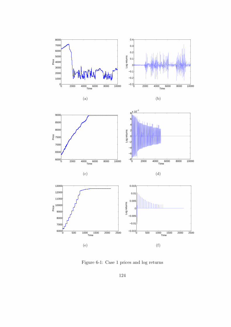
0 2000 4000 6000 8000 100000
1000
2000
3000
4000
5000
6000
7000
8000
Time
Pric
e
(a)
0 2000 4000 6000 8000 10000−0.3
−0.2
−0.1
0
0.1
0.2
0.3
0.4
Time
Log
retu
rns
(b)
0 2000 4000 6000 8000 100006000
6500
7000
7500
8000
8500
9000
Time
Pric
e
(c)
0 2000 4000 6000 8000 10000−8
−6
−4
−2
0
2
4
6
8x 10
−3
Time
Log
retu
rns
(d)
0 500 1000 1500 2000 25006000
7000
8000
9000
10000
11000
12000
13000
Time
Pric
e
(e)
0 500 1000 1500 2000 2500−0.015
−0.01
−0.005
0
0.005
0.01
0.015
Time
Log
retu
rns
(f)
Figure 6-1: Case 1 prices and log returns
124
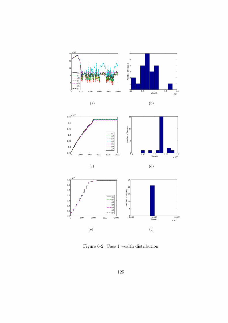
0 2000 4000 6000 8000 100004
6
8
10
12
14x 10
4
g1g2g3g4g5g6g7
(a)
0.6 0.8 1 1.2 1.4
x 105
0
1
2
3
4
5
6
Wealth
Num
ber
of T
rade
rs
(b)
0 2000 4000 6000 8000 100001.25
1.3
1.35
1.4
1.45
1.5
1.55x 10
5
g1g2g3g4g5g6g7
(c)
1.4 1.45 1.5 1.55 1.6
x 105
0
5
10
15
Wealth
Num
ber
of T
rade
rs
(d)
0 500 1000 1500 20001.2
1.3
1.4
1.5
1.6
1.7
1.8
1.9x 10
5
g1g2g3g4g5g6g7
(e)
1.8855 1.8855 1.8856
x 105
0
5
10
15
20
25
Wealth
Num
ber
of T
rade
rs
(f)
Figure 6-2: Case 1 wealth distribution
125
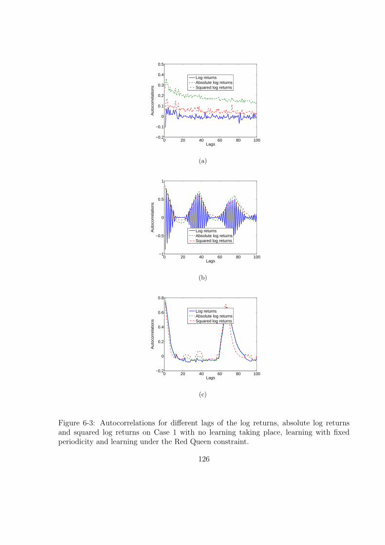
0 20 40 60 80 100−0.2
−0.1
0
0.1
0.2
0.3
0.4
0.5
Lags
Aut
ocor
rela
tions
Log returnsAbsolute log returnsSquared log returns
(a)
0 20 40 60 80 100−1
−0.5
0
0.5
1
Lags
Aut
ocor
rela
tions
Log returnsAbsolute log returnsSquared log returns
(b)
0 20 40 60 80 100−0.2
0
0.2
0.4
0.6
0.8
Lags
Aut
ocor
rela
tions
Log returnsAbsolute log returnsSquared log returns
(c)
Figure 6-3: Autocorrelations for different lags of the log returns, absolute log returnsand squared log returns on Case 1 with no learning taking place, learning with fixedperiodicity and learning under the Red Queen constraint.
126
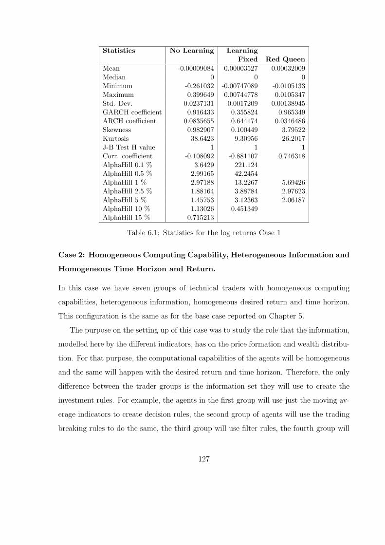
Statistics No Learning LearningFixed Red Queen
Mean -0.00009084 0.00003527 0.00032009Median 0 0 0Minimum -0.261032 -0.00747089 -0.0105133Maximum 0.399649 0.00744778 0.0105347Std. Dev. 0.0237131 0.0017209 0.00138945GARCH coefficient 0.916433 0.355824 0.965349ARCH coefficient 0.0835655 0.644174 0.0346486Skewness 0.982907 0.100449 3.79522Kurtosis 38.6423 9.30956 26.2017J-B Test H value 1 1 1Corr. coefficient -0.108092 -0.881107 0.746318AlphaHill 0.1 % 3.6429 221.124AlphaHill 0.5 % 2.99165 42.2454AlphaHill 1 % 2.97188 13.2267 5.69426AlphaHill 2.5 % 1.88164 3.88784 2.97623AlphaHill 5 % 1.45753 3.12363 2.06187AlphaHill 10 % 1.13026 0.451349AlphaHill 15 % 0.715213
Table 6.1: Statistics for the log returns Case 1
Case 2: Homogeneous Computing Capability, Heterogeneous Information and
Homogeneous Time Horizon and Return.
In this case we have seven groups of technical traders with homogeneous computing
capabilities, heterogeneous information, homogeneous desired return and time horizon.
This configuration is the same as for the base case reported on Chapter 5.
The purpose on the setting up of this case was to study the role that the information,
modelled here by the different indicators, has on the price formation and wealth distribu-
tion. For that purpose, the computational capabilities of the agents will be homogeneous
and the same will happen with the desired return and time horizon. Therefore, the only
difference between the trader groups is the information set they will use to create the
investment rules. For example, the agents in the first group will use just the moving av-
erage indicators to create decision rules, the second group of agents will use the trading
breaking rules to do the same, the third group will use filter rules, the fourth group will
127

use the volatility, the fifth will use a momentum indicator, the sixth a moving average
indicator based on the momentum and the last group will use all the indicators.
Figures 6-4(a) and 6-4(b) show the price and log returns without learning taking place.
The next two figures 6-4(c) and 6-4(d) show the price and log returns when learning with
fixed periodicity takes place. Finally, figures 6-4(e) and 6-4(f) show the price and log
returns when the Red Queen constraint is applied.
In this case, we can see that having traders with more computing capability creates
more interesting price dynamics. Additionally, we can observe the impact that the het-
erogeneity in the use of information has on the price dynamics. It is perceivable from
Figure 6-4 that more realistic price dynamics emerged in comparison with Case 1 and
that the log returns present volatility clustering in the three different cases.
In Figure 6-5 we can observe the wealth evolution and the wealth distribution in the
final round for the Case 2 in three different scenarios: without learning taking place
(figures 6-5(a) and 6-5(b)), when learning with fixed periodicity is happening (figures
6-5(c) and 6-5(d)) and when the Red Queen Constraint is being activated (figures 6-5(e)
and 6-5(f)). In this figure we can appreciate that there is a diverse wealth evolution
by group when learning is not happening and that there is a certain convergence when
learning takes place, specially under the Red Queen Constraint.
Figure 6-6 shows the autocorrelation for different lags of Case 2. In such figure, we
can see that the autocorrelations for the experiments where learning does not take place,
behave in a realistic way to a certain extent (in particular the autocorrelations of the
log returns). When learning in a fixed way takes place, the autocorrelations behave less
reasonable, with the autocorrelation of the squared returns being practically zero for all
lags. The case where the Red Queen constraint is applied is the one that reports the
best behaviour for all the autocorrelations. We observed in the Red Queen constraint
experiment that there is a positive autocorrelation of the absolute and squared log returns
for short lags, even the decay for such case is quite acceptable.
Table 6.3 shows the statistics corresponding to the second of the analyzed cases. We
128
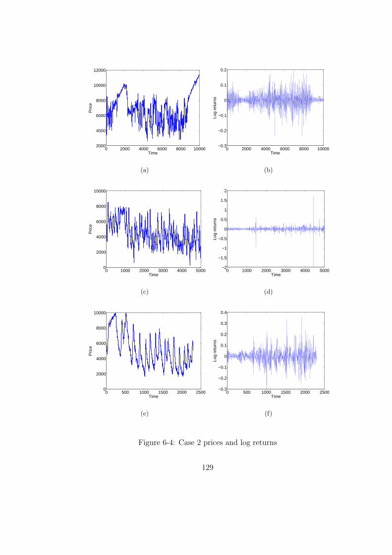
0 2000 4000 6000 8000 100002000
4000
6000
8000
10000
12000
Time
Pric
e
(a)
0 2000 4000 6000 8000 10000−0.3
−0.2
−0.1
0
0.1
0.2
Time
Log
retu
rns
(b)
0 1000 2000 3000 4000 50000
2000
4000
6000
8000
10000
Time
Pric
e
(c)
0 1000 2000 3000 4000 5000−2
−1.5
−1
−0.5
0
0.5
1
1.5
2
Time
Log
retu
rns
(d)
0 500 1000 1500 2000 25000
2000
4000
6000
8000
10000
Time
Pric
e
(e)
0 500 1000 1500 2000 2500−0.3
−0.2
−0.1
0
0.1
0.2
0.3
0.4
Time
Log
retu
rns
(f)
Figure 6-4: Case 2 prices and log returns
129
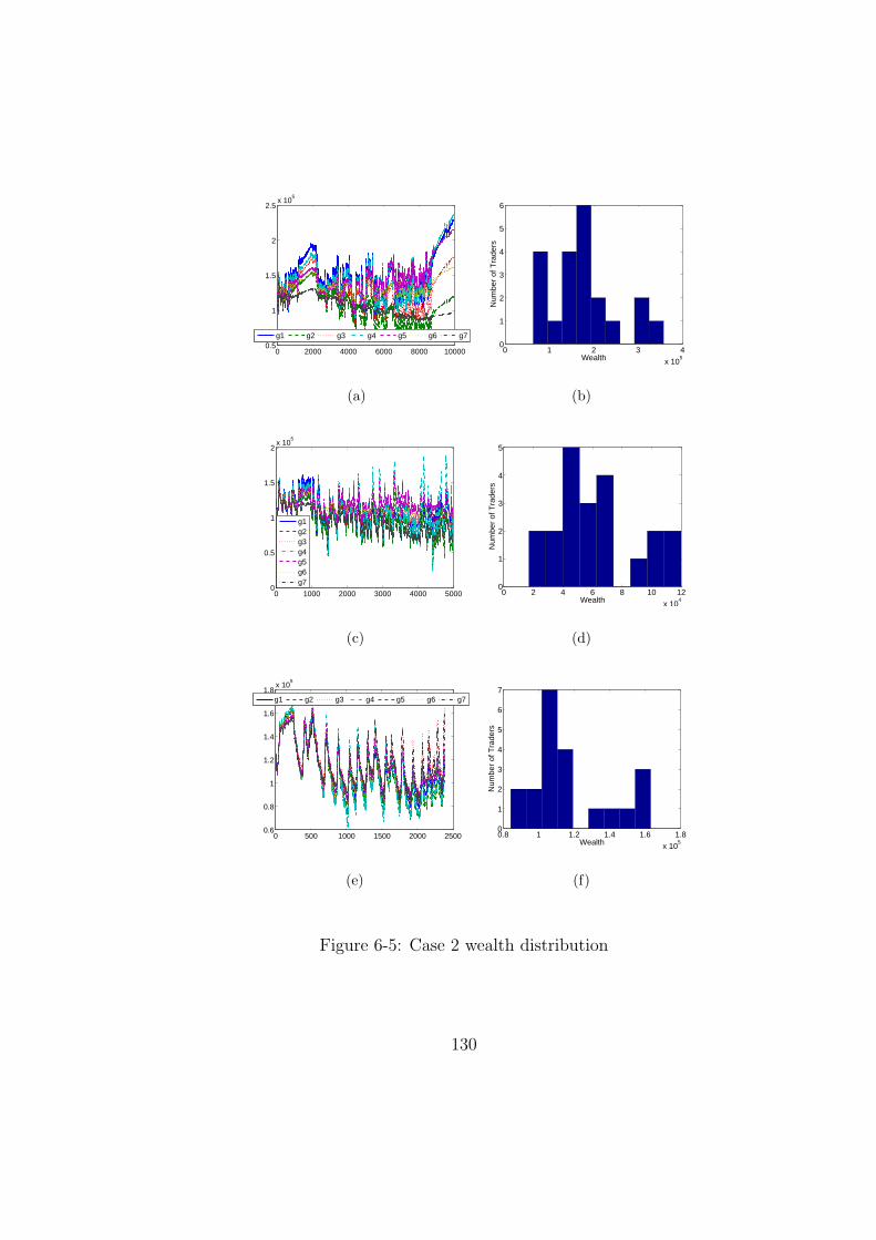
0 2000 4000 6000 8000 100000.5
1
1.5
2
2.5x 10
5
g1 g2 g3 g4 g5 g6 g7
(a)
0 1 2 3 4
x 105
0
1
2
3
4
5
6
Wealth
Num
ber
of T
rade
rs
(b)
0 1000 2000 3000 4000 50000
0.5
1
1.5
2x 10
5
g1g2g3g4g5g6g7
(c)
0 2 4 6 8 10 12
x 104
0
1
2
3
4
5
Wealth
Num
ber
of T
rade
rs
(d)
0 500 1000 1500 2000 25000.6
0.8
1
1.2
1.4
1.6
1.8x 10
5
g1 g2 g3 g4 g5 g6 g7
(e)
0.8 1 1.2 1.4 1.6 1.8
x 105
0
1
2
3
4
5
6
7
Wealth
Num
ber
of T
rade
rs
(f)
Figure 6-5: Case 2 wealth distribution
130
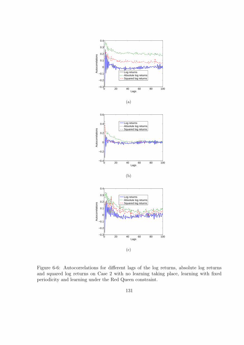
0 20 40 60 80 100−0.3
−0.2
−0.1
0
0.1
0.2
0.3
0.4
Lags
Aut
ocor
rela
tions
Log returnsAbsolute log returnsSquared log returns
(a)
0 20 40 60 80 100−0.4
−0.2
0
0.2
0.4
0.6
Lags
Aut
ocor
rela
tions
Log returnsAbsolute log returnsSquared log returns
(b)
0 20 40 60 80 100−0.3
−0.2
−0.1
0
0.1
0.2
0.3
0.4
Lags
Aut
ocor
rela
tions
Log returnsAbsolute log returnsSquared log returns
(c)
Figure 6-6: Autocorrelations for different lags of the log returns, absolute log returnsand squared log returns on Case 2 with no learning taking place, learning with fixedperiodicity and learning under the Red Queen constraint.
131
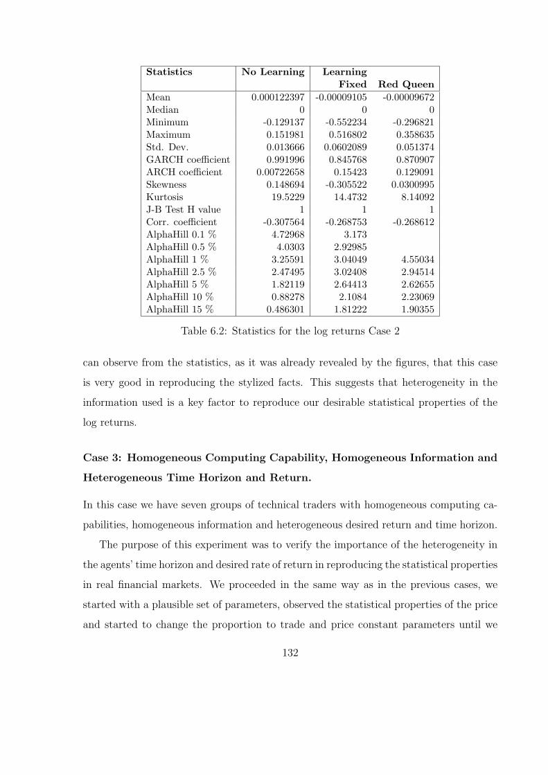
Statistics No Learning LearningFixed Red Queen
Mean 0.000122397 -0.00009105 -0.00009672Median 0 0 0Minimum -0.129137 -0.552234 -0.296821Maximum 0.151981 0.516802 0.358635Std. Dev. 0.013666 0.0602089 0.051374GARCH coefficient 0.991996 0.845768 0.870907ARCH coefficient 0.00722658 0.15423 0.129091Skewness 0.148694 -0.305522 0.0300995Kurtosis 19.5229 14.4732 8.14092J-B Test H value 1 1 1Corr. coefficient -0.307564 -0.268753 -0.268612AlphaHill 0.1 % 4.72968 3.173AlphaHill 0.5 % 4.0303 2.92985AlphaHill 1 % 3.25591 3.04049 4.55034AlphaHill 2.5 % 2.47495 3.02408 2.94514AlphaHill 5 % 1.82119 2.64413 2.62655AlphaHill 10 % 0.88278 2.1084 2.23069AlphaHill 15 % 0.486301 1.81222 1.90355
Table 6.2: Statistics for the log returns Case 2
can observe from the statistics, as it was already revealed by the figures, that this case
is very good in reproducing the stylized facts. This suggests that heterogeneity in the
information used is a key factor to reproduce our desirable statistical properties of the
log returns.
Case 3: Homogeneous Computing Capability, Homogeneous Information and
Heterogeneous Time Horizon and Return.
In this case we have seven groups of technical traders with homogeneous computing ca-
pabilities, homogeneous information and heterogeneous desired return and time horizon.
The purpose of this experiment was to verify the importance of the heterogeneity in
the agents’ time horizon and desired rate of return in reproducing the statistical properties
in real financial markets. We proceeded in the same way as in the previous cases, we
started with a plausible set of parameters, observed the statistical properties of the price
and started to change the proportion to trade and price constant parameters until we
132

obtained what we considered to be realistic prices.
In this experiment, for the first group of agents, we chose a small time horizon and a
desired rate of return that made sense for such time horizon (otherwise we would have
experienced the same problems that we had at the beginning of our research). For the
second group we chose a slightly bigger time horizon and again a desired rate of return
that was reasonable to expect in such time. We increased the time horizon and chose the
respective desired rate of return for the remaining five groups. With this organization,
we had the first groups with small time horizon and rate of return and the last groups
with the parameters taking bigger values.
Figures 6-7(a) and 6-7(b) show the price and log returns without learning taking place.
The next two figures 6-7(c) and 6-7(d) show the price and log returns when learning with
fixed periodicity takes place. Finally the figures 6-7(e) and 6-7(f) show the price and log
returns when the Red Queen constraint is applied.
We can observe that the obtained dynamics without learning are interesting and
realistic. However, when learning in a fixed way takes place, after certain time, there is
a sort of agreement and the volatility of the log return starts to decrease. When the Red
Queen Constraint is applied, the price exhibits volatility clustering as well and a decrease
on it as in the fixed learning case.
In Figure 6-8 we can observe the wealth evolution and the wealth distribution in the
final round for Case 3 in three different scenarios: without learning taking place (figures
6-8(a) and 6-8(d)), when learning with fixed periodicity is happening (figures 6-8(c) and
6-8(d)) and when the Red Queen Constraint is being activated (figures 6-8(e) and 6-
8(f)). From such figures we can see that in the case when learning does not take place,
the evolution of wealth of the different groups varies considerably. When fixed learning
takes place, most of the groups behave in the same way and such similar behaviour is
even stronger in the case of the Red Queen Constraint.
Figure 6-9 shows the autocorrelation for different lags of Case 3. In such figure we
can observe well behaved autocorrelations for the three different cases: when there is no
133
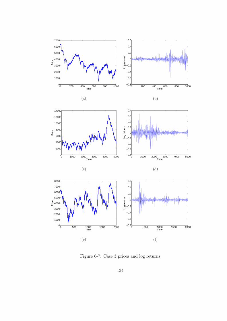
0 200 400 600 800 10000
1000
2000
3000
4000
5000
6000
7000
Time
Pric
e
(a)
0 200 400 600 800 1000−0.8
−0.6
−0.4
−0.2
0
0.2
0.4
0.6
Time
Log
retu
rns
(b)
0 1000 2000 3000 4000 50000
2000
4000
6000
8000
10000
12000
14000
Time
Pric
e
(c)
0 1000 2000 3000 4000 5000−0.4
−0.3
−0.2
−0.1
0
0.1
0.2
0.3
0.4
Time
Log
retu
rns
(d)
0 500 1000 1500 20000
1000
2000
3000
4000
5000
6000
7000
8000
Time
Pric
e
(e)
0 500 1000 1500 2000−0.8
−0.6
−0.4
−0.2
0
0.2
0.4
0.6
Time
Log
retu
rns
(f)
Figure 6-7: Case 3 prices and log returns
134
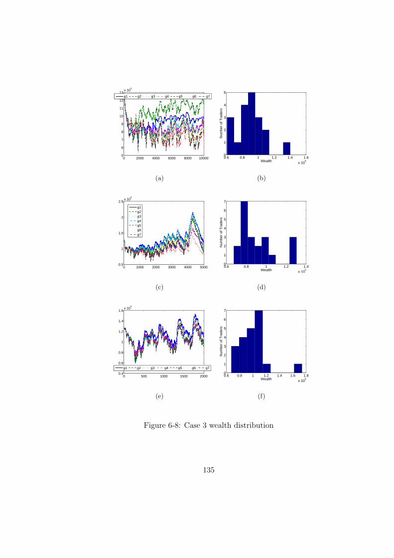
0 2000 4000 6000 8000 100005
6
7
8
9
10
11
12
13x 10
4
g1 g2 g3 g4 g5 g6 g7
(a)
0.6 0.8 1 1.2 1.4 1.6
x 105
0
1
2
3
4
5
Wealth
Num
ber
of T
rade
rs
(b)
0 1000 2000 3000 4000 50000.5
1
1.5
2
2.5x 10
5
g1g2g3g4g5g6g7
(c)
0.6 0.8 1 1.2 1.4
x 105
0
1
2
3
4
5
6
7
Wealth
Num
ber
of T
rade
rs
(d)
0 500 1000 1500 20000.4
0.6
0.8
1
1.2
1.4
1.6x 10
5
g1 g2 g3 g4 g5 g6 g7
(e)
0.6 0.8 1 1.2 1.4 1.6 1.8
x 105
0
1
2
3
4
5
6
7
Wealth
Num
ber
of T
rade
rs
(f)
Figure 6-8: Case 3 wealth distribution
135
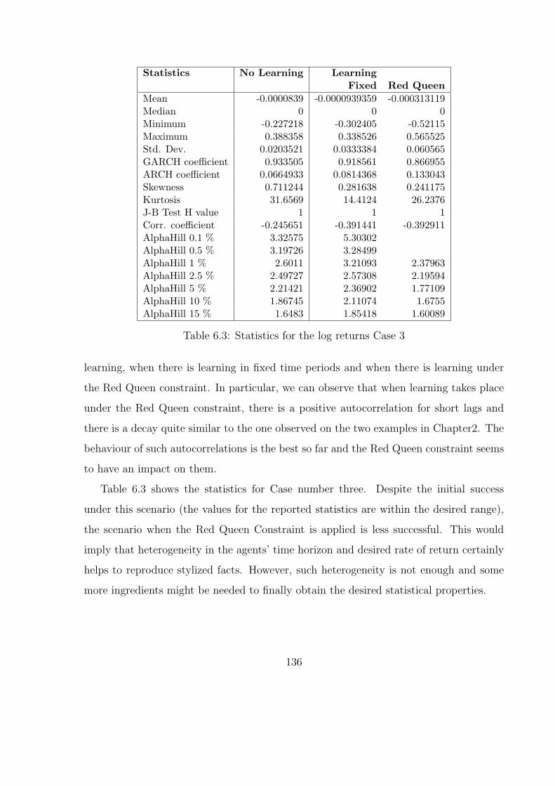
Statistics No Learning LearningFixed Red Queen
Mean -0.0000839 -0.0000939359 -0.000313119Median 0 0 0Minimum -0.227218 -0.302405 -0.52115Maximum 0.388358 0.338526 0.565525Std. Dev. 0.0203521 0.0333384 0.060565GARCH coefficient 0.933505 0.918561 0.866955ARCH coefficient 0.0664933 0.0814368 0.133043Skewness 0.711244 0.281638 0.241175Kurtosis 31.6569 14.4124 26.2376J-B Test H value 1 1 1Corr. coefficient -0.245651 -0.391441 -0.392911AlphaHill 0.1 % 3.32575 5.30302AlphaHill 0.5 % 3.19726 3.28499AlphaHill 1 % 2.6011 3.21093 2.37963AlphaHill 2.5 % 2.49727 2.57308 2.19594AlphaHill 5 % 2.21421 2.36902 1.77109AlphaHill 10 % 1.86745 2.11074 1.6755AlphaHill 15 % 1.6483 1.85418 1.60089
Table 6.3: Statistics for the log returns Case 3
learning, when there is learning in fixed time periods and when there is learning under
the Red Queen constraint. In particular, we can observe that when learning takes place
under the Red Queen constraint, there is a positive autocorrelation for short lags and
there is a decay quite similar to the one observed on the two examples in Chapter2. The
behaviour of such autocorrelations is the best so far and the Red Queen constraint seems
to have an impact on them.
Table 6.3 shows the statistics for Case number three. Despite the initial success
under this scenario (the values for the reported statistics are within the desired range),
the scenario when the Red Queen Constraint is applied is less successful. This would
imply that heterogeneity in the agents’ time horizon and desired rate of return certainly
helps to reproduce stylized facts. However, such heterogeneity is not enough and some
more ingredients might be needed to finally obtain the desired statistical properties.
136
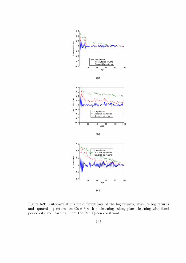
0 20 40 60 80 100−0.4
−0.3
−0.2
−0.1
0
0.1
0.2
0.3
Lags
Aut
ocor
rela
tions
Log returnsAbsolute log returnsSquared log returns
(a)
0 20 40 60 80 100−0.4
−0.3
−0.2
−0.1
0
0.1
0.2
0.3
0.4
Lags
Aut
ocor
rela
tions
Log returnsAbsolute log returnsSquared log returns
(b)
0 20 40 60 80 100−0.4
−0.2
0
0.2
0.4
0.6
Lags
Aut
ocor
rela
tions
Log returnsAbsolute log returnsSquared log returns
(c)
Figure 6-9: Autocorrelations for different lags of the log returns, absolute log returnsand squared log returns on Case 3 with no learning taking place, learning with fixedperiodicity and learning under the Red Queen constraint.
137
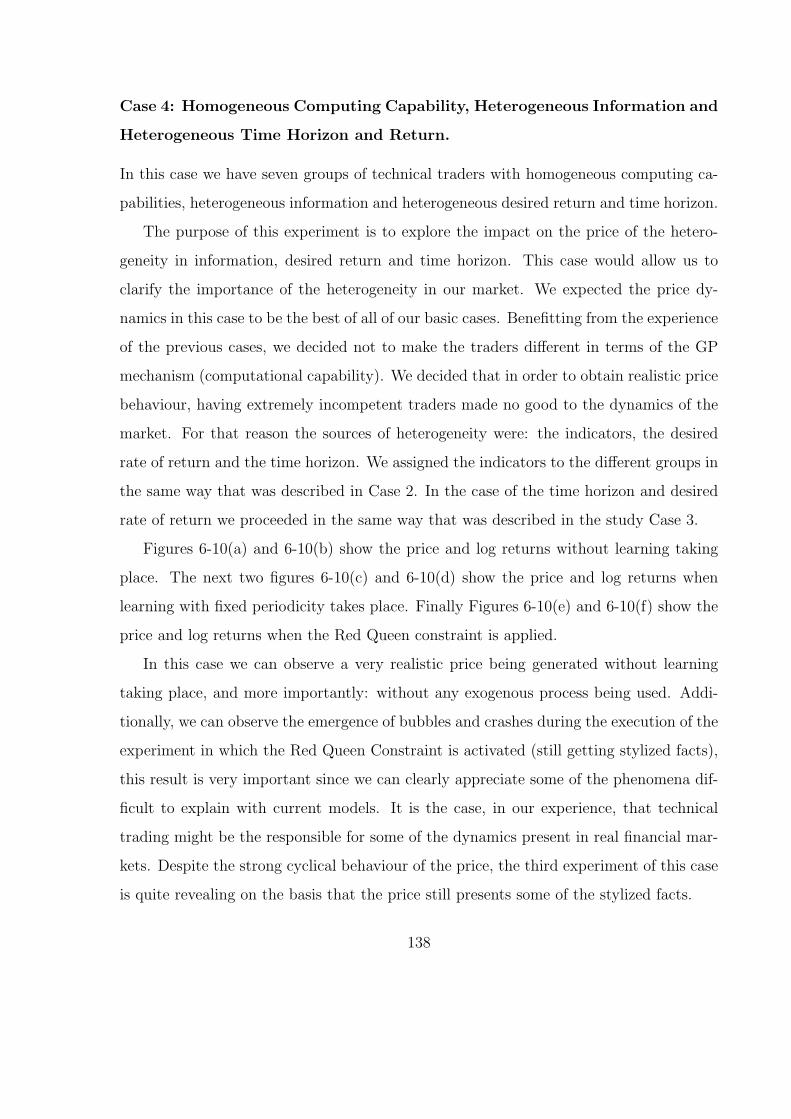
Case 4: Homogeneous Computing Capability, Heterogeneous Information and
Heterogeneous Time Horizon and Return.
In this case we have seven groups of technical traders with homogeneous computing ca-
pabilities, heterogeneous information and heterogeneous desired return and time horizon.
The purpose of this experiment is to explore the impact on the price of the hetero-
geneity in information, desired return and time horizon. This case would allow us to
clarify the importance of the heterogeneity in our market. We expected the price dy-
namics in this case to be the best of all of our basic cases. Benefitting from the experience
of the previous cases, we decided not to make the traders different in terms of the GP
mechanism (computational capability). We decided that in order to obtain realistic price
behaviour, having extremely incompetent traders made no good to the dynamics of the
market. For that reason the sources of heterogeneity were: the indicators, the desired
rate of return and the time horizon. We assigned the indicators to the different groups in
the same way that was described in Case 2. In the case of the time horizon and desired
rate of return we proceeded in the same way that was described in the study Case 3.
Figures 6-10(a) and 6-10(b) show the price and log returns without learning taking
place. The next two figures 6-10(c) and 6-10(d) show the price and log returns when
learning with fixed periodicity takes place. Finally Figures 6-10(e) and 6-10(f) show the
price and log returns when the Red Queen constraint is applied.
In this case we can observe a very realistic price being generated without learning
taking place, and more importantly: without any exogenous process being used. Addi-
tionally, we can observe the emergence of bubbles and crashes during the execution of the
experiment in which the Red Queen Constraint is activated (still getting stylized facts),
this result is very important since we can clearly appreciate some of the phenomena dif-
ficult to explain with current models. It is the case, in our experience, that technical
trading might be the responsible for some of the dynamics present in real financial mar-
kets. Despite the strong cyclical behaviour of the price, the third experiment of this case
is quite revealing on the basis that the price still presents some of the stylized facts.
138
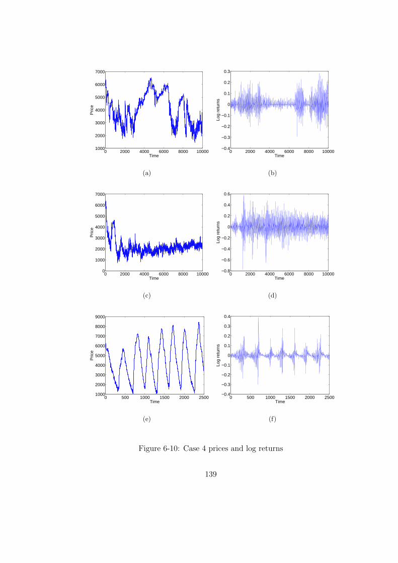
0 2000 4000 6000 8000 100001000
2000
3000
4000
5000
6000
7000
Time
Pric
e
(a)
0 2000 4000 6000 8000 10000−0.4
−0.3
−0.2
−0.1
0
0.1
0.2
0.3
Time
Log
retu
rns
(b)
0 2000 4000 6000 8000 100000
1000
2000
3000
4000
5000
6000
7000
Time
Pric
e
(c)
0 2000 4000 6000 8000 10000−0.8
−0.6
−0.4
−0.2
0
0.2
0.4
0.6
Time
Log
retu
rns
(d)
0 500 1000 1500 2000 25001000
2000
3000
4000
5000
6000
7000
8000
9000
Time
Pric
e
(e)
0 500 1000 1500 2000 2500−0.4
−0.3
−0.2
−0.1
0
0.1
0.2
0.3
0.4
Time
Log
retu
rns
(f)
Figure 6-10: Case 4 prices and log returns
139
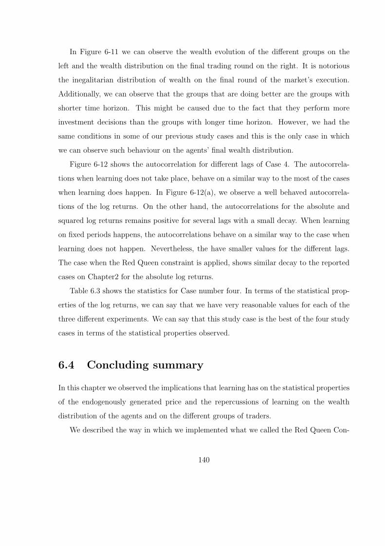
In Figure 6-11 we can observe the wealth evolution of the different groups on the
left and the wealth distribution on the final trading round on the right. It is notorious
the inegalitarian distribution of wealth on the final round of the market’s execution.
Additionally, we can observe that the groups that are doing better are the groups with
shorter time horizon. This might be caused due to the fact that they perform more
investment decisions than the groups with longer time horizon. However, we had the
same conditions in some of our previous study cases and this is the only case in which
we can observe such behaviour on the agents’ final wealth distribution.
Figure 6-12 shows the autocorrelation for different lags of Case 4. The autocorrela-
tions when learning does not take place, behave on a similar way to the most of the cases
when learning does happen. In Figure 6-12(a), we observe a well behaved autocorrela-
tions of the log returns. On the other hand, the autocorrelations for the absolute and
squared log returns remains positive for several lags with a small decay. When learning
on fixed periods happens, the autocorrelations behave on a similar way to the case when
learning does not happen. Nevertheless, the have smaller values for the different lags.
The case when the Red Queen constraint is applied, shows similar decay to the reported
cases on Chapter2 for the absolute log returns.
Table 6.3 shows the statistics for Case number four. In terms of the statistical prop-
erties of the log returns, we can say that we have very reasonable values for each of the
three different experiments. We can say that this study case is the best of the four study
cases in terms of the statistical properties observed.
6.4 Concluding summary
In this chapter we observed the implications that learning has on the statistical properties
of the endogenously generated price and the repercussions of learning on the wealth
distribution of the agents and on the different groups of traders.
We described the way in which we implemented what we called the Red Queen Con-
140
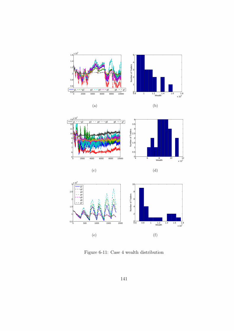
0 2000 4000 6000 8000 100000.4
0.6
0.8
1
1.2
1.4
1.6x 10
5
g1 g2 g3 g4 g5 g6 g7
(a)
0.8 1 1.2 1.4 1.6 1.8
x 105
0
1
2
3
4
5
Wealth
Num
ber
of T
rade
rs
(b)
0 2000 4000 6000 8000 100005
6
7
8
9
10
11
12
13x 10
4
g1 g2 g3 g4 g5 g6 g7
(c)
4 6 8 10 12
x 104
0
0.5
1
1.5
2
2.5
3
3.5
4
Wealth
Num
ber
of T
rade
rs
(d)
0 500 1000 1500 20000.5
1
1.5
2
2.5
3x 10
5
g1g2g3g4g5g6g7
(e)
0.6 0.8 1 1.2 1.4 1.6 1.8
x 105
0
2
4
6
8
10
Wealth
Num
ber
of T
rade
rs
(f)
Figure 6-11: Case 4 wealth distribution
141
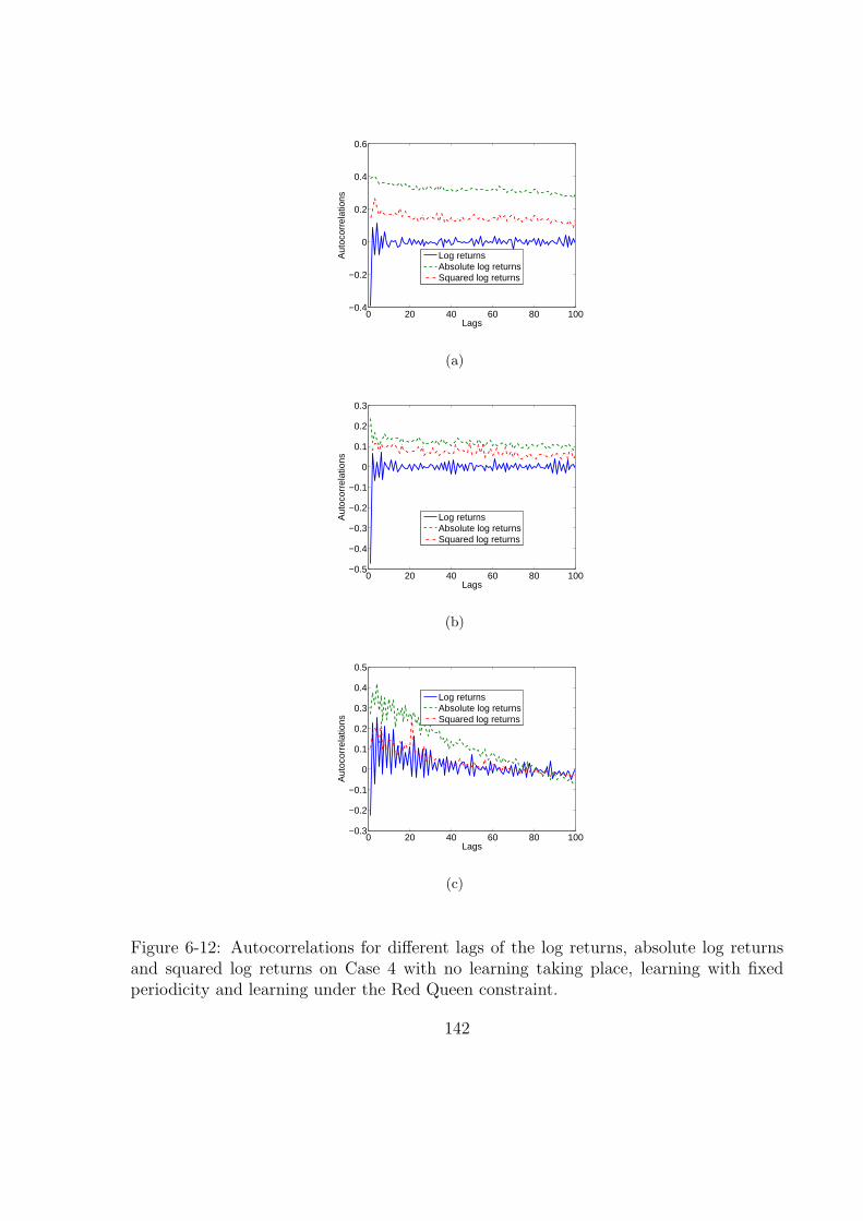
0 20 40 60 80 100−0.4
−0.2
0
0.2
0.4
0.6
Lags
Aut
ocor
rela
tions
Log returnsAbsolute log returnsSquared log returns
(a)
0 20 40 60 80 100−0.5
−0.4
−0.3
−0.2
−0.1
0
0.1
0.2
0.3
Lags
Aut
ocor
rela
tions
Log returnsAbsolute log returnsSquared log returns
(b)
0 20 40 60 80 100−0.3
−0.2
−0.1
0
0.1
0.2
0.3
0.4
0.5
Lags
Aut
ocor
rela
tions
Log returnsAbsolute log returnsSquared log returns
(c)
Figure 6-12: Autocorrelations for different lags of the log returns, absolute log returnsand squared log returns on Case 4 with no learning taking place, learning with fixedperiodicity and learning under the Red Queen constraint.
142
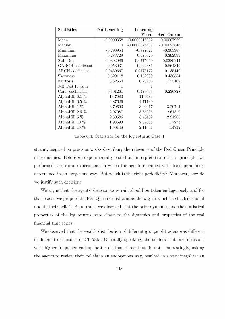
Statistics No Learning LearningFixed Red Queen
Mean -0.0000358 -0.0000916302 0.00007929Median 0 -0.0000826437 -0.00023846Minimum -0.293954 -0.777021 -0.303987Maximum 0.283729 0.575629 0.392999Std. Dev. 0.0892986 0.0775069 0.0389244GARCH coefficient 0.953031 0.922381 0.864849ARCH coefficient 0.0469667 0.0776172 0.135149Skewness 0.329118 0.152999 0.438554Kurtosis 8.62664 6.23266 17.5102J-B Test H value 1 1 1Corr. coefficient -0.391261 -0.473053 -0.236828AlphaHill 0.1 % 13.7083 11.6683AlphaHill 0.5 % 4.87626 4.71139AlphaHill 1 % 3.79693 3.94017 3.29714AlphaHill 2.5 % 2.97087 3.85935 2.61319AlphaHill 5 % 2.60586 3.48402 2.21265AlphaHill 10 % 1.98593 2.52688 1.7273AlphaHill 15 % 1.56148 2.11641 1.4732
Table 6.4: Statistics for the log returns Case 4
straint, inspired on previous works describing the relevance of the Red Queen Principle
in Economics. Before we experimentally tested our interpretation of such principle, we
performed a series of experiments in which the agents retrained with fixed periodicity
determined in an exogenous way. But which is the right periodicity? Moreover, how do
we justify such decision?
We argue that the agents’ decision to retrain should be taken endogenously and for
that reason we propose the Red Queen Constraint as the way in which the traders should
update their beliefs. As a result, we observed that the price dynamics and the statistical
properties of the log returns were closer to the dynamics and properties of the real
financial time series.
We observed that the wealth distribution of different groups of traders was different
in different executions of CHASM: Generally speaking, the traders that take decisions
with higher frequency end up better off than those that do not. Interestingly, asking
the agents to review their beliefs in an endogenous way, resulted in a very inegalitarian
143

distribution of wealth in the final trading round of the market. This result is a very
interesting one, since we are just asking to the population of traders to do the best they
can to preserve their status quo in the market. Nevertheless, it seems that such arms
race causes the majority of the traders to end up with a small amount of wealth, while
very few agents end up with most of the population’s wealth.
Additionally, we observed that heterogeneity does help in general terms to obtain
realistic statistical properties. However, having heterogeneity in computing capability
between the agents proved to be harmful to our intentions of reproducing realistic market
dynamics (Case 1). This point is important for us due to the fact that we believe that
simulations of Artificial Financial Markets should be done with agents capable enough
to imitate human behaviour. In our experience, having agents with not good enough
investment decision rules, creates a very different type of market dynamics.
Information proved to be an interesting source of heterogeneity in our market (Case
2). The impact of the time horizon and desired rate of return was beneficial (Case 3).
The combination of heterogeneity in both information and investment preferences did
not lead to the best results in terms of reproducing the stylized facts (Case 4).
In real life, the traders are likely to have different time horizons (due to budget
constraints or simple preferences), return considerations and they tend to look in different
ways the same information (or even they might use different sources of information).
Nevertheless, it is unlikely that there is a big difference in computing capability among
the main players (small investors and the rest of us are just noise).
We should emphasize at this point that despite the fact that our market is capable
of modelling fundamental behaviour, in this four study cases we are not making use of
it. This means that we are able to mimic to a certain extent the statistical properties of
log returns without an explicit-exogenous fundamental mechanism. We consider this to
be very important for the study of Artificial Financial Markets because so far we have
always seen a sort of fundamental mechanism in any of the important works in this field.
The exception to this rule are the works [42], [82] and [88]. In [42] the authors arrive to
144

C1 C2 C3 C4 C5 C6 C7Case 1 with no learning 3 3 3 7 3 7 7
Case 1 with fixed learning 3 3 3 7 7 7 7
Case 1 with Red Queen constraint 3 3 3 3 7 7 7
Case 2 with no learning 3 3 3 3 3 7 7
Case 2 with fixed learning 3 3 3 3 3 7 7
Case 2 with Red Queen constraint 3 3 3 3 3 7 7
Case 3 with no learning 3 3 3 3 3 7 3
Case 3 with fixed learning 3 3 3 3 3 7 3
Case 3 with Red Queen constraint 3 3 3 3 3 3 7
Case 4 with no learning 3 3 3 3 3 7 3
Case 4 with fixed learning 3 3 3 3 3 7 7
Case 4 with Red Queen constraint 3 3 3 3 3 7 7
Table 6.5: Evaluation criteria on stock prices for each group of experiments.
a conclusion that is very much related to ours:
“This suggests that the statistics we observe in real markets is mainly due to
the interaction among speculators trading on technical grounds, regardless of
economic fundamentals”
Finally, we resume in the same way as it was done on Chapter 5, the criteria that we
used to differentiate the results of the experiments reported on this chapter. We use the
same criteria also defined on the previous chapter. In Table 6.4, we can observe which
of the individual criterion is satisfied by each study case. We can see that the cases that
satisfy the most of the criteria are: the three experiments of Case 3 and the experiment
in which learning does not take place of the Case 4. The Case 3 is the most successful
of all the study cases and it is the only case in which the price satisfies C6. In Case 4
we can observe that in the experiment with the Red Queen Constraint the non-linear
autocorrelations decay to zero. However, in the case of the absolute log returns, such
autocorrelation becomes negative for lags close to 100.
145
Chapter 7
Conclusions
In this chapter we summarize the research done so far, we review the experimental results,
describe our contributions to the field and propose possible lines of future research.
7.1 Summary
Artificial financial markets of all sorts and flavors have been developed in the last decade
and are still being created with an always increasing complexity and proximity to reality
that was not possible in the past. The research in this field is now mature and its
acceptance in Economics has finally increased.
Motivated by the richness of this area of research, we decided to participate in it and
to stretch some particular aspects of this methodology. The main research goals at the
start of this project were:
• to gain better understanding of the way in which market efficiency is achieved inour model.
• to identify the sort of conditions that are necessary to reproduce the stylized factsof the stock returns with an artificial market.
To help us achieve these goals, we have implemented a Co-evolutionary Heterogeneous
Artificial Stock Market (CHASM) platform which incorporates non-simple agents and a
146
behavioural constraint among other important features. We decided to model as close
as possible (but also as generic as possible) the behaviour that the traders present in the
real markets. We did not want to make strong assumptions about the agents’ behaviour,
expectations, rationality or risk perception. Neither we wanted to implement specific
markets. Those are the reasons why the strategic behaviour of our agents is very rich
and non-simple. Additionally, we studied the way in which the wealth is distributed
among the agents as a result of changes in the adaptation and competition between
them.
We considered that technical analysis should be a key feature of our agents’ behaviour,
despite the open debate between some academics and some practitioners about it. To
justify our decision, we are convinced that technical analysis is an important tool for
decision making in financial investments. Besides, there is a strong evidence that technical
analysis is being used extensively in financial markets [109], [157], [186]. Furthermore,
there are numerous studies that support the profitability of technical analysis in financial
markets [5], [34], [38], [212], [61], [63], [64], [62], [103], [158], [159].
With the elements we had at hand, we took the decision of using EDDIE ([41], [195],
[131], [194], [196], [148], [199], [197] ) as the basic framework to design the investment
strategy of our agents. We chose EDDIE because it has been proven to be a successful
tool to support investment decision making. The task seemed to be not too complicated,
considering our experience in financial forecasting using technical analysis and the vast
literature on artificial financial markets. Nevertheless, the price dynamics that our first
models exhibited were not realistic at all and we observed either a monotonous price
behaviour or an always increasing (decreasing) trend on the price.
Early experiments showed us that a straightforward implementation of EDDIE traders
with a simple market mechanism was not sufficient to get stylized facts. Moreover,
reproducing the statistical properties of real financial markets required a lot of work and
the exploration of several characteristics of the model. For that reason we decided to
incorporate some other features into our market. Such phenomena is related to what
147

Edmonds and Moss describe very well in [70].They argue that it is still common in multi-
agent modeling to take an existing algorithm (designed with other purpose in mind) and
use it for the cognition of the agent, regardless of whether this can be justified in terms
of what is known about the behaviour of the modelled entities.
We included another two kinds of market participants: value investors and noise
traders. Additionally, we enhanced the technical traders with some other features. For
example, we included the feature consisting of a fundamental-like behaviour under certain
specific circumstances and also included stop-loss and profit-taking limit orders as part
of a more complete investment strategy.
In our approach, we believe that the source of complexity of the model is the strategic
behaviour of the agents and not the market mechanism or at least that is our intention.
In fact, we did not make any strong assumptions and maintained a very simple market
mechanism during the whole process of modifications. After modifying the model and of a
deep investigation of the behaviour of our market, we arrived to a particular configuration
that we considered to be the base case for the exploration of the characteristics of our
model.
Figure 5-1, in Chapter 5, illustrates the exploration of some characteristics of our
artificial market. At the centre, we can see what we call the base case; such case is
the one in which we successfully observed stylized facts without the agents adapting to
the new conditions of the market (learning). We considered that this case was a good
starting point to explore the other characteristics of the model. From there, we changed
one by one different parameters and mechanisms of the model to observe the changes on
the price and wealth distribution of the agents.
After success with the new enhancements and the discovered configuration of the
market, we decided to create several basic cases to study the impact of the learning
process on the market dynamics. We studied the returns and the wealth distribution of
the agents as well.
148
7.2 Experiments summary
As we explained on the previous section, we developed a series of experiments in which we
explored the different parameters of our model and key changes in some other elements
that compose our artificial market. Judging from the results of the experiments described
in Chapters 4, 5 and 6, the most important conclusions that we can make about such
experiments will be explained in detail in the following sections.
7.2.1 Initial training
The initial phase of training was important in order to generate agents with realistic
behaviour. At the beginning of the project we did not put enough emphasis on the
desired rate of return for a given time horizon. Given our chosen rate of return and
time horizon, the classes on the training data were heavily unbalanced. For example, if
we asked an unreasonable high return for an unreasonable short time horizon, the class
with the highest frequency was the HOLD one. Obviously, the kind of decision trees
(investment rules) that were generated by the evolutionary process were trees whose
most likely recommendation was to HOLD. This is a well known problem in machine
learning and we had to solve it before going any further on the research.
Given the experience gained on the importance of the initial training, we decided
to create heterogeneous groups of agents whose desired rate of return and time horizon
caused the training data to be equally split on the three different classes (BUY, SELL
and HOLD). For example, if a trader wants to achieve a 3% return, she must have a time
horizon of at least 5 days because in real financial data changes by 3% over 5 or fewer
days are rare; if she wants to get a 4% return, she must wait at least for 7 days because of
the few cases present in real financial time series. Otherwise, we could have the classes on
the training data highly unbalanced and that would have biased the evolutionary search.
149
7.2.2 Learning and wealth
Learning must have helped to improve the trader’s wealth if we were to study its impact
on artificial markets. This was a crucial issue for us. In order to prove the importance
of learning, we conducted a series of experiments in which we replicated one trader and
allowed her to retrain during the simulation of the market. The rest of the traders
remained without changes, i.e. without retraining. Afterwards, we compared the wealth
of both the original trader and the replicated one. To be able to generalize from this
experiments, we performed this task for different traders in different groups. The results
in the majority of the cases proved that learning does help to improve performance on
wealth terms.
In Figure 4.5 we can see some examples of the experiments mentioned above. In such
figure we can see the wealth evolution during the trading of the replicated trader (dashed
line) and the original one (solid line). We can see that in Figure 4-3(a), learning did not
improve the wealth of the replicated trader, even after retraining on the 1000th period.
However, after approximately the 2500th period, the replicated trader is better-off than
the original one. In the rest of the reported examples, the improvement is clearer than in
the previously mentioned example. We can clearly see in Figures 4-3(b), 4-3(c), 4-3(d)
how learning improved the replicated agent’s wealth.
7.2.3 Fitness measure
The fitness function, based on the rate of correctness of the GP mechanism, can be used
to drive the agent’s learning process. This result might sound obvious but it cannot
be assumed to be always true, as the rate of correctness of the agents’ GP mechanism
(working as a classifier) is not necessarily translated into the agents’ wealth. The results
mentioned in the previous section can be used to justify this point, because we used the
rate of correctness for the learning processes.
An alternative GP mechanism is to use the profit as the fitness measure. This type
of fitness measure has been successfully used in some other works like [35], [68], [67].
150
7.2.4 Heterogeneity
One of the things that microeconomics teaches you is that individuals are not alike. There
is heterogeneity, and probably the most important heterogeneity here is heterogeneity of
expectations. If we didn’t have heterogeneity, there would be no trade. But developing an
analytic model with heterogeneous agents is difficult. (Ken Arrow, In: D. Colander, R.P.F.
Holt and J. Barkley Rosser (eds.), The Changing Face of Economics. Conversations with
Cutting Edge Economists. The University of Michigan Press, Ann Arbor, 2004, pp 301.)
Heterogeneity is important for the properties of the simulated returns. By using
CHASM we could model heterogeneity in different forms, including: information, com-
puting capability, desired rate of return and time horizon, fundamental-like behaviour,
generation of limit orders, etc.
The different sources of heterogeneity had different effects on the properties of the
price and the returns. The experiments described in Chapters 5 and 6 may give us a
clear idea of such effects. For example, heterogeneity in the information used by the
agents is useful; on the other hand, heterogeneity in computing capability is irrelevant.
We can see as an example the price and log-returns of the experiments performed with
heterogeneous computational capabilities. Figures 6-1(a) and 6-1(b) present executions
in which there is heterogeneity in computing capability and there is no learning. Figures
6-1(c) and 6-1(d) show the same case when learning in fixed periods takes place. Lastly,
Figures 6-1(e) and 6-1(f) show the same configuration when the Red Queen constraint is
in place.
7.2.5 Learning and returns
The learning mechanism does change the statistical properties of the returns. Moreover,
we can observe the implications of programming the traders with fixed and Red Queen
retraining on the results of the experiments described in Chapter 6. We can observe that,
despite the fact that the simulated prices behave closely to the real prices, when learning
happens the properties of the returns reproduce more closely the stylized facts.
151

Figures 6-1, 6-4, 6-7 and 6-10 can give us a better idea of the impact that learning
has on the price and return. The Tables 6.3, 6.3, 6.3, 6.3 show the statistics for the cases
illustrated in such figures. In such tables we can observe that the statistics in general are
close to the statistics present in real financial markets and when learning happens, the
dynamics become even more realistic.
7.2.6 The Red Queen Principle
The implementation of the behavioural constraint known in this work as the Red Queen
constraint is an important component of our model. There have been previous attempts
to model the necessity for adaptation to the new conditions on the environment as seen
in [53] and [119]. However, we are convinced that the necessity of adaptation should
be defined endogenously. The results reported in Chapter 6 show the difference on the
statistical properties of the returns without learning, with learning in fixed periods and
with learning driven by the Red Queen constraint. The results show that learning driven
by such constraint has a more beneficial impact on the statistical properties of the log-
returns in relation with the other two cases.
7.3 Contributions
The major contributions of our research are:
• We have implemented a flexible platform called CHASM, to support a wide range
of experiments. It is a comprehensive platform and we have proven its flexibility,
by conducting different kinds of detailed experiments. CHASM allowed us to study
the relevant factors which can lead to certain market dynamics.
• CHASM allows us to model heterogeneous, realistic and non-simple market agents.
In CHASM we can explore the impact of changes on the proportions of different
152
types of traders. Additionally, we can change easily the numerous parameters that
rule the technical traders’ behaviour.
• We have studied the impact of agents’ learning in CHASM. Moreover, we have
demonstrated that even in an artificial environment, learning by a GP forecasting
mechanism (EDDIE) can improve an agent’s performance.
• By using CHASM we found a set of conditions under which some stylized facts
emerge under a simple market mechanism even with no fundamental trading taking
place.
• We developed an endogenous behavioural constraint using “The Red Queen prin-
ciple”, that allowed us to model the fierce competition in real financial markets in
the search for profits.
• CHASM has allowed us to carefully study the role of heterogeneity in our model
by allowing us to organize groups with different characteristics and parameters.
In CHASM, we are able to model heterogeneity in information, computational
capability and desired return and time horizon.
We consider that a realistic behaviour in the modelling of artificial agents, hetero-
geneity and behavioural constraints are the main factors to achieve realistic statistical
properties of the endogenously generated price. We obtained some stylized facts even
with a very simple market mechanism. However, some more work is needed to avoid, or
at least to understand, the cyclical behaviour of the price that emerged in the third and
forth study cases reported on Chapter 6.
7.3.1 CHASM
The implemented platform CHASM was designed from the beginning with two important
objectives from the Software Engineering point of view:
153

• The platform should be easy to extend and modify
• The platform should be flexible to allow us to model different phenomena.
After several changes and extensions, the platform has proven to achieve the original
objectives. Furthermore, it has even been enriched with a useful Graphic User Interface
(GUI). Therefore, the platform in addition to accomplish its original objectives is easy
to use.
Some other important characteristics of the platform are related to the GP mecha-
nism. First, we had to change our implementation of the GP mechanism from a purist
object oriented one to a more efficient implementation due to the fact that we would
have dozens of such mechanisms running at the same time. Second, we implemented a
very efficient method to avoid bloat and to speed up our simulation, see [164]. Bloat
happens during the evolutionary process, when the trees grow in size but there is little
improvement in fitness, see [116]. Essentially, this means that there are some branches
of the trees that are redundant or even worse, they reduce the fitness of the individual.
We considered that the control of bloat is important because it was necessary for us
to generate realistic investment rules. It would be very difficult for us (and for anyone)
to justify very complex rules being used by the agents.
7.3.2 Agents
The different types of artificial financial markets that currently exist can vary widely on
several aspects: market mechanism, type of agents, learning, time, securities, etc.
We decided to focus our research on what we considered to be two important aspects:
the modelling of realistic traders and the implications of a co-evolutionary principle on
the price formation process.
The debate is still very intense about the role that technical analysis plays in today’s
financial markets but it is undeniable, at least from the practitioners point of view, its
154
importance in such markets. In Section 4.5 we have demonstrated that technical analysis
at least helps to improve performance in our artificial market.
The approach that we have followed in this research is on the opposite side of the spec-
trum in relation with the research done in [91] and [184]. We believe and we have demon-
strated it to a certain extent that the plausible modelling of intelligence and adaptation
of our agents create “realistic” price dynamics even with a simple market mechanism.
We are not saying that the market mechanism is not important on the formation on the
price dynamics. However, we believe that the behaviour of the economic agents plays a
significant role as well. Moreover, the continuous adaptation to the new conditions of
the market has an important change on the price properties.
We agree more with the conclusions drawn in [57]. In such work Cliff and Bruten
argue that the success (which seems to be apparent) of zero-intelligence constrained
agents could be predicted by the probabilistic analysis of the system. More behavioural
(justifiable) sophistication should be added to the agents to realistically test the behaviour
of humans in different markets.
7.3.3 Learning in CHASM
In some works in Agent-Based simulations, it is assumed that the agents will be suc-
cessful in the task that they are assigned for or that learning will work on their benefit.
Unfortunately, there are not many works in which the authors can certify that learning is
making them any good (or at least is not doing them any harm). We have conducted very
precise series of experiments in which we could clearly verify that the learning mechanism
is improving the agents’ situation on the environment.
Despite the fact that the price is generated endogenously and that all the environment
is dynamically affected by the agents, the learning mechanism that we have implemented
is doing well the task for which it was designed for.
It is worth saying that we have experimentally proved that a fitness measure based
on the rate of correctness can be translated into wealth improvement of the agents in an
155
ever changing environment.
7.3.4 CHASM and Stylized Facts
At the end of our project, we have found a set of conditions under which stylized facts
arise in our model. Such conditions provide us with a clear idea of which are the factors
that matter in the simulation of financial markets. To answer such question is not a
trivial matter, as it has been pointed out in [42] by Caldarelli, Marsili and Zhang:
“It is clear that by no means one can conclude that our model captures all
the relevant aspects of a real market. As already said it misses the effects of
external drive. More importantly, it does not contain adaptive dynamics of
the players strategies. Further studies should answer the question: what are
the essential elements in a model that will reproduce realistic results?”
We performed two sets of experiments. First, we worked in an environment where
the agents did not learn and we found the setting by which the dynamics of the returns
replicated the real markets. Second, we performed the same task in an environment in
which two different frequencies of learning took place; again we found the setting in which
some stylized facts emerged.
7.3.5 The Red Queen principle
The concept of market efficiency is of central importance in the area of Financial Eco-
nomics, see [71] and [72]. The concept is not new and has been changing recently but
it is always under the constant scrutiny due to the empirical evidence that apparently
contradicts such efficiency (or at least some forms of efficiency), see [174], [175]. However,
little is said about how such efficiency is achieved. There exists empirical evidence about
the different degrees of efficiency of the various financial markets in the world and we
believe that fierce competition is at the centre of such property of the markets.
156
We have achieved the replication of some of the empirical properties of financial
markets, helped by an ingeniously designed behavioural constraint. We have carefully
investigated the effects of a plausible way of driving the speed of adaptation of the market
participants.
7.3.6 The role of heterogeneity
When some research is argued to be inspired on the Agent-based methodology, it is
inferred that the agents are heterogeneous. However, the degree or forms of heterogeneity
are not easy to determine in most of the cases. In our experience, heterogeneity proved
to be a key factor in the success of our simulation. We can certainly say that (a) the
organization of the market in different types of agents and (b) within those types of agents
the existence of different heterogeneous groups; contributed heavily to the reproduction
of stylized facts in our simulated market.
Interestingly, having heterogeneity on the computing capabilities of the agents, proved
to be against the desired statistical properties of the market. The cases of the simulated
market least successful in reproducing the stylized facts, were those involving heterogene-
ity of the GP mechanism. This again goes against the line of research taken in [91] and
[184]. We believe that the lack of interesting dynamics in the above mentioned experi-
ments is related to the absence of realism in the building of the agents’ strategies, caused
by the limited computing capability endowed to some of the agents.
We are convinced that zero-intelligence agents or agents with a similar type of in-
telligent behaviour, are not the way forward in this field. Some not very gifted traders
are present in real financial markets for sure but it is impossible to model a realistic
market just with such type of agents. In our case, more interesting price dynamics arose
when we included competent enough agents and more heterogeneity between them. In
[88], the authors have also identified the presence of heterogeneity as a key mechanism
to reproduce some of the statistical properties of the financial returns.
The majority of the agent-based markets do not consider heterogeneity on the time
157
horizon of the agents. CHASM allows us to model different expectations about the price
(expected return) and different time horizons in which the agents expect such change in
price. In [118], LeBaron suggests that the incorporation of short and long term investors
is desirable to model in a more realistic manner the markets.
To finalize this section lets just say that in real markets and in real life, people commit
mistakes, have different opinions and different forecasts. Such differences might well be
the cause for trading in financial markets. This heterogeneity is difficult to model with
traditional methods in which the common assumptions are that the individuals are fully
rational and have common expectations.
7.4 Future research
One obvious way in which our work can be extended is to model more realistic and
complex market mechanisms. Despite the fact that the artificially generated price satisfies
some of our original requirements, it is necessary to analyze the impact of the market
mechanism in an environment that already satisfies some of the desirable properties
of such type of simulations. More work is needed to get prices that mach closer the
behaviour of real prices. The first natural candidate is the double auction market. Once
such market is implemented with the present agents, a more in deep investigation of the
statistical properties of the generated price could be conducted.
On Market Microstructure is where some of the most intense and challenging re-
search is being made. The comparison between different market mechanisms is always
an attractive line of research. Which sort of market favours more the dissemination of
information? Which market mechanism is more efficient?
Going even further, some other market participants like market makers could be
incorporated into our framework. There is currently some interesting research already
done modelling artificial market makers [47]. Unfortunately, their work is different to
ours on the type of traders used. It is understandable to focus on the modelling of the
158
market maker and to make her a realistic and non-simple agent, however we should not
compromise the modelling of the other (the traders) market participants.
More experiments can be conducted to study the co-evolution of the agents or some
other means of interaction between the agents could be provided to study some interesting
behavioural phenomena thought to be present in modern financial markets. Some recent
research has gone along the lines of behavioural finance and artificial markets like in
[35]. We believe that it is an interesting and promising avenue of research. Artificial
Financial Markets can be controlled beyond any experiments with real humans and they
can certainly include non-simple trading techniques that are currently being used in real
markets. Moreover, it is required a flexible and transparent tool to model the behavioural
aspects and learning of the agents. We are convinced that GP is the right tool to do so,
as we have proven in CHASM.
In recent years automatic trading has been increasing dramatically in different mar-
kets and financial markets are not the exception. What are the implications of such
trading in financial markets? What is the effect of increasing intensive computing on the
search for arbitrage opportunities? Is this sort of trading going to increase the volatility
of the prices or to increase the likelihood of financial crashes?
Financial markets are becoming an ever changing environment with automatic trad-
ing using powerful computer hardware and novel algorithms, better heuristics, and new
statistical methods. Can we feel the presence of the Red Queen around? Are not financial
markets the ultimate laboratory for competitive co-evolution?
Those are the sort of questions in which Agent-Based Artificial Financial Markets are
able to provide some understanding beyond the analytical methods. Moreover, those are
the sort of questions that will require heterogeneous agents with a realistic behaviour, a
flexible learning mechanism and biologically inspired endogenous constraints.
159
Bibliography
[1] B. Alexandrova-Kabadjova, A. Krause, and E. Tsang. An agent-based model of
interactions in the payment card market. Working Paper 07, Centre Computational
Finance and Economic Agents, March 2006.
[2] B. Alexandrova-Kabadjova, E. Tsang, and A. Krause. Market structure and in-
formation in payment card markets. Working Paper 06, Centre Computational
Finance and Economic Agents, March 2006.
[3] S. Alfarano, F. Wagner, and T. Lux. A minimal noise trader model with realistic
time series properties. Economics Working Paper 2003–15, University of Kiel,
Germany, 2003.
[4] S. Alfarano, F. Wagner, and T. Lux. Estimation of agent-based models: the case
of an asymmetric herding model. Technical report, University of Kiel, Germany,
July 2004.
[5] F. Allen and R. Karjalainen. Using genetic algorithms to find technical trading
rules. Journal of Financial Economics, 51:245–271, 1999.
[6] M. Amin. Restructuring the electric enterprise: Simulating the evolution of the
electric power industry with intelligent adaptive agents. In A. Faruqui and K. Eakin,
editors, Market Analysis and Resource Management, chapter 3. Kluwer Publishers,
March 2002.
160
[7] P. Angeline. Genetic Programming and Emergent Intelligence. In K. E. Kinnear,
Jr., editor, Advances in Genetic Programming, chapter 4, pages 75–98. MIT Press,
1994.
[8] J. Arifovic. Genetic algorithm learning and the cobweb model. Journal of Economic
Dynamics & Control, 18:3–28, 1994.
[9] J. Arifovic. The behavior of the exchange rate in the genetic algorithm and exper-
imental economics. Journal of Political Economy, 104:510–541, 1996.
[10] J. Arifovic. Evolutionary Model of the Exchange Rate Behavior. Computing in
Economics and Finance 1999 611, Society for Computational Economics, March
1999.
[11] J. Arifovic. Evolutionary Dynamics of Currency Substitution. Journal of Economic
Dynamics & Control, 25:395–417, March 2001.
[12] W. B. Arthur. LEARNING AND ADAPTIVE ECONOMIC BEHAVIOR. Design-
ing Economic Agents that Act Like Human Agents: A Behavioral Approach to
Bounded Rationality. American Economic Review, 81:353–359, May 1991.
[13] W. B. Arthur. On learning and adaptation in the economy. Working paper 92-07-
038, Santa Fe Institute, 1992.
[14] W. B. Arthur. Inductive reasoning and bounded rationality: The El Farol problem.
American Economic Review, 84:406–411, May 1994.
[15] W. B. Arthur. Out-of-equilibrium economics and agent-based modeling. In K. Judd
and L. Tesfatsion, editors, Handbook of Computational Economics, Volume 2:
Agent-Based Computational Economics,. Elsevier Science B.V., 2005.
[16] W. B. Arthur, J. H. Holland, B. LeBaron, R. G. Palmer, and P. Talyer. Asset
pricing under endogenous expectations in an artificial stock market. In W. B.
161
Arthur, S. Durlauf, and D. Lane, editors, The Economy as an Evolving Complex
System II. Addison-Wesley, 1997.
[17] M. Ausloos and K. Ivanova. Mechanistic approach to generalized technical analysis
of share prices and stock market indices. Euro Physics Journal B, 27:177–187,
2002.
[18] M. Austin, G. Bates, M. Dempster, and S. Williams. Adaptive systems for foreign
exchange trading. Eclectic, 18:21–26, Autumn 2004.
[19] M. P. Austin, G. Bates, M. A. H. Dempster, V. Leemans, and S. N. Williams.
Adaptive systems for foreign exchange trading. Quantitative Finance, 4(4):37–45,
August 2004.
[20] R. Axelrod. The evolution of strategies in the iterated prisoner’s dilemma. In
L. Davis, editor, Genetic algorithms and simulated annealing, pages 32–41. Pit-
man/Morgan Kaufmann, London/Los Altos, CA, 1987.
[21] R. Axelrod. Advancing the art of simulation in the social sciences. In R. Conte,
R. Hegselmann, and P. Terna, editors, Simulating Social Phenomena, pages 21–40.
Springer-Verlag, Berlin, 1997.
[22] R. Axelrod. Agent-based modeling as a bridge between disciplines. In K. Judd and
L. Tesfatsion, editors, Handbook of Computational Economics, Volume 2: Agent-
Based Computational Economics. Elsevier Science B.V., 2005.
[23] R. Axelrod and L. Tesfatsion. A guide for newcomers to agent-based modeling in the
social sciences. In K. Judd and L. Tesfatsion, editors, Handbook of Computational
Economics, Volume 2: Agent-Based Computational Economics. Elsevier Science
B.V., 2005.
[24] E. M. Azoff and E. M. Azoff. Neural Network Time Series Forecasting of Financial
Markets. John Wiley & Sons, Inc., New York, NY, USA, 1994.
162
[25] P. Bak, M. Paczuski, and M. Shubik. Price variations in a stock market with many
agents. Physica A, 246:430–453, 1997.
[26] A. V. Banerjee. A simple model of herd behavior. The Quarterly Journal of
Economics, 107:797–817, Agust 1992.
[27] N. Barberis, A. shleifer, and R. W. Vishny. A model of investor sentiment. Working
Paper 5926, National Bureau of Economic Research, February 1997.
[28] R. A. Batchelor and G. A. Albanis. Predicting high performance stocks us-
ing dimensionality reduction techniques based on neural networks. In C. Dunis
and A. Timmerman, editors, Developments in Forecast Combination and Portfolio
Choice, pages 117–134. Kluwer Academic Publishers, 2001.
[29] R. J. Bauer. Genetic Algorithms and Investment Strategies. John Wiley & Sons,
1994.
[30] L. A. Becker and M. Seshadri. Gp-evolved technical trading rules can outperform
buy and hold. In Sixth International Conference on Computational Intelligence
and Natural Computing, Embassy Suites Hotel and Conference Center, Cary, North
Carolina USA, 26-30 Sept. 2003.
[31] J. M. Benitez, J. L. Castro, and I. Requena. Are artificial neural networks black
boxes? IEEE Transactions on Neural Networks, 8:1156–1164, 1997.
[32] S. Bikhchandani, D. Hirshleifer, and I. Welch. A theory of fads, fashion, custom,
and cultural change as informational cascades. The Journal of Political Economy,
100:992–1026, October 1992.
[33] S. Bikhchandani and S. Sharma. Herd behavior in financial markets: A review.
IMF Working Paper 00/48, International Monetary Fund, March 2000.
[34] L. Blume, D. Easley, and M. O’Hara. Market statistics and technical analysis: The
role of volume. Journal of Finance, 49:151–181, March 1994.
163
[35] H. P. Boswijk, C. H. Hommes, and S. Manzan. Behavioral heterogeneity in stock
prices. In IFAC symposium Computational Economics, Finance and Engineering,
Seattle, USA, 28-30 June 2003.
[36] T. Brenner. Agent learning representation advice in modelling economic learning.
In K. Judd and L. Tesfatsion, editors, Handbook of Computational Economics,
Volume 2: Agent-Based Computational Economics,. Elsevier Science B.V., 2005.
[37] W. Brock and C. H. Hommes. A rational route to randomness. Econometrica,
65:1059–1095, 1997.
[38] W. Brock, J. Lakonishok, and B. LeBaron. Simple technical trading rules and the
stochastic properties of stock returns. Journal of Finance, 47:1731–1764, December
1992.
[39] J. Bullard, J. Arifovic, and J. Duffy. Learning in a model of economic growth and
development. Working Paper 1995-017A, Federal Reserve Bank Of St. Louis, 1995.
[40] J. Bullard and J. Duffy. Using genetic algorithms to model the evolution of het-
erogeneous beliefs. Computational Economics, 13:41–60, February 1999.
[41] J. M. Butler and E. P. K. Tsang. EDDIE beats the bookies. Technical Report
CSM-259, Computer Science, University of Essex, Colchester CO4 3SQ, UK, 15
Dec. 1995.
[42] G. Caldarelli, M. Marsili, and Y.-C. Zhang. A prototype model of stock exchange.
Europhysics Letters, 40:479–484, December 1997.
[43] L. Cao and F. E. Tay. Financial forecasting using support vector machines. Neural
Computing & Applications, 10:184–192, May 2001.
[44] L. Cao and F. E. Tay. Support vector machine with adaptive parameters in financial
time series forecasting. IEEE Transactions on Neural Networks, 14:1506–1518,
November 2006.
164
[45] D. Challet, M. Marsili, and Y.-C. Zhang. Modeling market mechanism with mi-
nority game. Physica A, 276:284–315, 2000.
[46] N. T. Chan, B. LeBaron, A. W. Lo, and T. Poggio. Agent-based models of financial
markets: A comparison with experimental markets. MIT Sloan Working Paper
4195-01, Massachusetts Institute of Technology, October 2001.
[47] N. T. Chan and C. R. Shelton. An electronic market maker. Technical Report
200-005, MIT Artificial Intelligence Laboratory, 2001.
[48] S.-H. Chen, editor. Genetic Algorithms and Genetic Programming in Computa-
tional Finance. Kluwer Academic, 2002.
[49] S.-H. Chen. Computational intelligence in economics and finance: Carrying on the
legacy of herbert simon. Information Sciences, 170:121–131, February 2005.
[50] S.-H. Chen. Editorial: Computationally intelligent agents in economics and finance.
Inf. Sci., 177(5):1153–1168, 2007.
[51] S.-H. Chen and C.-H. Yeh. Genetic programming learning in the cobweb model
with speculators. In International Computer Symposium (ICS’96). Proceedings of
International Conference on Artificial Intelligence, pages 39–46, National Sun Yat-
Sen University, Kaohsiung, Taiwan, R.O.C., 19-21 1996.
[52] S.-H. Chen and C.-H. Yeh. Using genetic programming to model volatility in
financial time series. In J. R. Koza, K. Deb, M. Dorigo, D. B. Fogel, M. Garzon,
H. Iba, and R. L. Riolo, editors, Genetic Programming 1997: Proceedings of the
Second Annual Conference, pages 58–63, Stanford University, CA, USA, 13-16 1997.
Morgan Kaufmann.
[53] S.-H. Chen and C.-H. Yeh. Evolving traders and the business school with genetic
programming: A new architecture of the agent-based artificial stock market. Jour-
nal of Economic Dynamics & Control, 25(3-4):363–393, March 2001.
165
[54] S.-H. Chen and C.-H. Yeh. On the emergent properties of artificial stock markets:
the efficient market hypothesis and the rational expectations hypothesis. Journal
of Economic Behavior & Organization, 49(2):217–239, 2002.
[55] C. Chiarella and X. Z. He. Asset price and wealth dynamics under heterogeneous
expectations. Quantitative Finance, 1:509–526, 2001.
[56] S. Cincotti, L. Ponta, and M. Raberto. A multi-assets artifcial stock market with
zero-intelligence traders. In WEHIA 2005 (13-15 June 2005), Essex, United King-
dom, 2005.
[57] D. Cliff and J. Bruten. Zero is not enough: On the lower limit of agent intelligence
for continuous double auction markets. In First Hewlett Packard International
Workshop on Interacting Software Agents, Bristol, United Kingdom, 1997.
[58] D. Cliff and G. F. Miller. Tracking the Red Queen: Measurements of Adaptive
Progress in Co-Evolutionary Simulations. In Proceedings of the Third European
Conference on Advances in Artificial Life, pages 200–218, London, UK, 1995.
Springer-Verlag.
[59] R. Cont. Empirical properties of asset returns: stylized facts and statistical issues.
Quantitative Finance, 1(2):223–236, February 2001.
[60] R. Cont and J.-P. Bouchaud. Herd behavior and aggregate fluctuations in financial
markets. Macroeconomic Dynamics, 4:170–196, 2000.
[61] M. A. H. Dempster and C. M. Jones. A real-time adaptive trading system using
genetic programming. Quantitative Finance, 1:397–413, 2000.
[62] M. A. H. Dempster and V. Leemans. An automated FX trading system using
adaptive reinforcement learning. Expert Systems with Applications, 30(3):543–552,
Apr. 2006. Special Issue on Financial Engineering.
166
[63] M. A. H. Dempster, T. W. Payne, Y. Romahi, and G. W. P. Thompson. Com-
putational learning techniques for intraday FX trading using popular technical
indicators. IEEE Transactions on Neural Networks, 12(4):744–754, July 2001.
[64] M. A. H. Dempster and Y. S. Romahi. Intraday FX trading: An evolutionary
reinforcement learning approach. In H. Yin, N. M. Allinson, R. T. Freeman, J. A.
Keane, and S. J. Hubbard, editors, Proceedings of Third International Conference
on Intelligent Data Engineering and Automated Learning - IDEAL 2002, volume
2412 of Lecture Notes in Computer Science, pages 347–358, Manchester, 12-14 Aug.
2002. Springer.
[65] K. Doerner, W. J. Gutjahr, R. F. Hart, C. Strauss, and C. Stummer. Pareto ant
colony optimization: A metaheuristic approach to multiobjective portfolio selec-
tion. Annals of Operations Research, 131:79–99, October 2004.
[66] J. Duffy. Agentbased models and human subject experiments. In K. Judd and
L. Tesfatsion, editors, Handbook of Computational Economics, Volume 2: Agent-
Based Computational Economics,. Elsevier Science B.V., 2005.
[67] B. Edmonds. Gossip, sexual recombination and the el farol bar: modelling the
emergence of heterogeneity. Artificial Societies and Social Simulation, 2, 1999.
[68] B. Edmonds. Modelling bounded rationality in agent-based simulations using the
evolution of mental models. In T. Brenner, editor, Computational Techniques for
Modelling Learning in Economics, pages 305–332. Kluwer, 1999.
[69] B. Edmonds and S. Moss. Modelling bounded rationality using evolutionary tech-
niques. In Evolutionary Computing, AISB Workshop, pages 31–42, 1997.
[70] B. Edmonds and S. Moss. The importance of representing cognitive processes in
multi-agent models. In G. Dorffner, H. Bischof, and K. Hornik, editors, Proceedings
of the International Conference in Artificial Neural Networks (ICANN), volume
2130, pages 759–766, Vienna, 2001. Springer Lecture Notes in Computer Science.
167
[71] E. F. Fama. Efficient capital markets: A review of theory and empirical work. The
Journal of Finance, 23:383–417, 1970.
[72] E. F. Fama. Efficient capital markets II. The Journal of Finance, 46:1575–1617,
December 1991.
[73] E. F. Fama and K. French. The cross-section of expected stock returns. The Journal
of Finance, 47:427–466, 1992.
[74] E. F. Fama and K. French. Size and book-to-market factors in earnings and stock
returns. The Journal of Finance, 50:131–155, 1995.
[75] A. Fan and M. Palaniswami. Selecting bankruptcy predictors using a support vector
machineapproach. In IEEE-INNS-ENNS International Joint Conference on Neural
Networks, 2000, volume 6, pages 354–359, 2000.
[76] J. Farmer and S. Joshi. The price dynamics of common trading strategies. SFI
Working Paper 00-12-069, Santa Fe Institute, 2000.
[77] J. D. Farmer. Market force, ecology, and evolution. Industrial and Corporate
Change, 11:895–953, November 1998.
[78] J. D. Farmer. Physicists attempt to scale the ivory towers of finance. Computing
In Science & Engineering, pages 26–39, November/December 1999.
[79] J. D. Farmer, P. Patelli, , and I. I. Zovko. The predictive power of zero intelligence
in financial markets. Proceedings of the National Academy of Sciences of the United
States of America, 102:2254–2259, February 2005.
[80] J. Ferber. Multi-agent Systems: An Introduction to Distributed Artificial Intelli-
gence. Addison-Wesley, 1999.
[81] S. Focardi, S. Cincotti, and M. Marchesi. Self-organization and market crashes.
Journal of Economic Behavior & Organization, 49:241–267, 2002.
168
[82] F. Franci and L. Matassini. Life in the stockmarket - a realistic model for trading,
2000.
[83] A. L. Garcia-Almanza and E. P. Tsang. Forecasting stock prices using genetic pro-
gramming and chance discovery. In 12th International Conference On Computing
In Economics And Finance, 2006.
[84] A. L. Garcia-Almanza and E. P. Tsang. The repository method for chance discov-
ery in financial forecasting. In Springer-Verlag, editor, KES2006 10th International
Conference on Knowledge-Based and Intelligent Information and Engineering Sys-
tems, 2006.
[85] A. L. Garcia-Almanza and E. P. Tsang. Simplifying decision trees learned by
genetic algorithms. In IEEE World Congress on Computational Intelligence, 2006.
[86] T. V. Gestel, B. Baesens, J. A. K. Suykens, M. Espinoza, D.-E. Baestaens, J. Van-
thienen, and B. D. Moor. Bankruptcy prediction with least squares support vector
machine classifiers. In IEEE International Conference on Computational Intelli-
gence for Financial Engineering, 2003, pages 1–8, March 2003.
[87] T. V. Gestel, J. A. K. Suykens, D.-E. Baestaens, A. Lambrechts, G. Lanckriet,
B. Vandaele, B. D. Moor, and J. Vandewalle. Financial time series prediction
using least squares support vector machines within the evidence framework. IEEE
Transactions On Neural Networks, 12:809–821, July 2001.
[88] F. Ghoulmie, R. Cont, and J.-P. Nadal. Heterogeneity and feedback in an agent-
based market model. Journal of Physics: Condensed Matter, 17:S1259–S1268,
2005.
[89] I. Giardina and J.-P. Bouchaud. Bubbles, crashes and intermittency in agent based
market models. The European Physical Journal B - Condensed Matter, 31:421–437,
2003.
169
[90] M. Gilli and P. Winker. A global optimization heuristic for estimating agent based
models. Computational Statistics & Data Analysis, 42:299–312, 2003.
[91] D. K. Gode and S. Sunder. Allocative efficiency of markets with zero intelligence
(z1) traders: Market as a partial substitute forindividual rationality. GSIA Working
Papers 1992-16, Carnegie Mellon University, Tepper School of Business, 1991.
[92] C. Goodwin and J. Heritage. Conversation analysis. Annual Review of Anthropol-
ogy, 19:283–307, 1990.
[93] M. Grinblatt and S. Titman. Performance measurement without benchmarks: An
examination of mutual fund returns. Journal of Business, 66(1):47–68, January
1993.
[94] M. Grinblatt, S. Titman, and R. Wermers. Momentum investment strategies, port-
folio performance, and herding: A study of mutual fund behavior. American Eco-
nomic Review, 85(5):1088–1105, December 1995.
[95] R. Grothmann. Multi-agent market modeling based on neural networks. PhD thesis,
Faculty of Economics, University of Bremen, 2002.
[96] S. Gutjahr, M. Riedmiller, and J. Klingemann. Daily Prediction of the For-
eign Exchange Rate Between the US Dollar and the German Mark using Neural
Networks. In Joint PACES / SPICES Conference Proceedings, pages 492–498.
Springer, February 1997.
[97] F. B. Hanson and J. J. Westman. Computational methods for portfolio and con-
sumption optimization in log-normal diffusion, log-uniform jump environments. In
Proceedings of the 15th International Symposium on Mathematical Theory of Net-
works and Systems, 12 August 2002, 2002.
[98] S. Hayward. Genetically optimised artificial neural network for financial time se-
170
ries data mining. Computing in Economics and Finance 2006 417, Society for
Computational Economics, July 2006.
[99] A. Heppenstall, A. Evans, and M. Birkin. Using hybrid agent-based systems to
model spatially-influenced retail markets. Journal of Artificial Societies and Social
Simulation, 9, 2006.
[100] B. M. Hill. A simple general approach to inference about the tail of a distribution.
Annals of Statistics, 3:1163–1173, 1975.
[101] J. H. Holland. Adaptation in Natural and Artificial Systems. University of Michigan
Press, Ann Arbor, MI, 1975.
[102] J. H. Holland and J. H. Miller. Artificial adaptive agents in economic theory. The
American Economic Review, 81:365–370, May 1991.
[103] P.-H. Hsu and C.-M. Kuan. Reexamining the profitability of technical analysis with
data snooping checks. Journal of Financial Econometrics, 3:606–628, 2005.
[104] W. Huang, Y. Nakamori, and S.-Y. Wang. Forecasting stock market movement
direction with support vector machine. Computers & Operations Research, 2004.
[105] Z. Huang, H. Chen, C.-J. Hsu, W.-H. Chen, and S. Wu. Credit rating analysis
with support vector machines and neural networks: a market comparative study.
Decision Support Systems, 37:543–558, 2004.
[106] K. Izumi and K. Ueda. Phase transition in a foreign exchange market-analysis
based on an artificial market approach. IEEE Trans. Evolutionary Computation,
5(5):456–470, 2001.
[107] P. Jefferies, M. Hart, P. Hui, and N. Johnson. From market games to real-world
markets. The European Physical Journal B - Condensed Matter and Complex Sys-
tems, 20:493–501, 2001 April.
171
[108] H. Juille and J. B. Pollack. Dynamics of co-evolutionary learning. In P. Maes,
M. J. Mataric, J.-A. Meyer, J. Pollack, and S. W. Wilson, editors, Proceedings of
the Fourth International Conference on Simulation of Adaptive Behavior: From
animals to animats 4, pages 526–534, Cape Code, USA, 9-13 Sept. 1996. MIT
Press.
[109] K. A. Kavajecz and E. R. Odders-White. Technical analysis and liquidity provision,
2002.
[110] A. P. Kirman. Whom or What Does the Representative Individual Represents?
The Journal of Economic Perspectives, 6:117–136, 1992.
[111] A. P. Kirman. Ants, rationality and recruitment. The Quarterly Journal of Eco-
nomics, 108:137–156, February 1993.
[112] A. P. Kirman and N. J. Vriend. Evolving market structure: An ace model of price
dispersion and loyalty. Journal of Economic Dynamics & Control, 25:459–502,
2001.
[113] J. Koza. Genetic Programming: On the Programming of Computers by Means of
Natural Selection. The MIT Press, Cambridge, Massachusetts, 1992.
[114] J. R. Koza. Evolution and co-evolution of computer programs to control
independent-acting agents. In J.-A. Meyer and S. W. Wilson, editors, From Ani-
mals to Animats: Proceedings of the First International Conference on Simulation
of Adaptive Behavior, 24-28, September 1990, pages 366–375, Paris, France, 1991.
MIT Press.
[115] J. Lakonishok, A. Shleifer, and R. W. Vishny. Contrarian investment, extrapola-
tion, and risk. The Journal of Finance, 49:1541–1578, December 1994.
[116] W. B. Langdon and R. Poli. Fitness causes bloat. In P. K. Chawdhry, R. Roy, and
172
R. K. Pant, editors, Soft Computing in Engineering Design and Manufacturing,
pages 13–22, London, 1997. Springer-Verlag.
[117] W. B. Langdon and R. Poli. Foundations of Genetic Programming. Springer-Verlag,
2002.
[118] B. LeBaron. A builder’s guide to agent based financial markets. Quantitative
Finance, 1:254–261, 2001.
[119] B. LeBaron. Empirical regularities from interacting long- and short-memory in-
vestors in an agent-based stock market. In IEEE Transactions on Evolutionary
Computation, volume 5 of 5, October 2001.
[120] B. LeBaron. Evolution and time horizons in an agent-based stock market. Macroe-
conomic Dynamics, 5:225–254, 2001.
[121] B. LeBaron. Calibrating an agent-based financial market. Working paper, Graduate
School of International Economics and Finance, Brandeis University, March 2003.
[122] B. LeBaron. Agent-based computational finance. In K. Judd and L. Tesfatsion,
editors, Handbook of Computational Economics, Volume 2: Agent-Based Compu-
tational Economics. Elsevier Science B.V., 2005.
[123] B. LeBaron. Agent-based financial markets: Matching stylized facts with style.
In D. C. Colander, editor, Post Walrasian Macroeconomics Beyond the Dynamic
Stochastic General Equilibrium Model. Cambridge University Press, Cambridge,
UK, July 2006.
[124] B. LeBaron, W. B. Arthur, and R. G. Palmer. Time series properties of an artificial
stock market. Journal of Economic Dynamics & Control, 23:1487–1516, September
1999.
[125] C. M. C. Lee and B. Swaminathan. Price momentum and trading volume. working
paper, Cornell University, 1999.
173
[126] W. Leigh, R. Purvis, and J. M. Ragusa. Forecasting the NYSE composite index
with technical analysis, pattern recognizer, neural networks, and genetic algorithm:
a case study in romantic decision support. Decision Support Systems, 32:361–377,
March 2002.
[127] J. M. Levine, L. B. Resnick, and E. T. Higgins. Social foundations of cognition.
Annual review of psychology, 44:585–612, 1993.
[128] H. Levy, M. Levy, and S. Solomon. Microscopic Simulation of Financial Markets:
From Investor Behavior to Market Phenomena. Academic Press, 2000.
[129] M. Levy, H. Levy, and S. Solomon. A microscopic model of the stock market:
cycles, booms and crashes. Economics Letters, 45:103–111, 1994.
[130] M. Levy and S. Solomon. Dynamical explanation for the emergence of power law in
a stock market model. International Journal of Modern Physics C, 7:65–72, 1996.
[131] J. Li and E. P. K. Tsang. Investment decision making using FGP: A case study.
In P. J. Angeline, Z. Michalewicz, M. Schoenauer, X. Yao, and A. Zalzala, editors,
Proceedings of the Congress on Evolutionary Computation, volume 2, pages 1253–
1259, Mayflower Hotel, Washington D.C., USA, 6-9 July 1999. IEEE Press.
[132] J. Li and E. P. K. Tsang. Reducing failures in investment recommendations us-
ing genetic programming. In Computing in Economics and Finance, Universitat
Pompeu Fabra, Barcelona, Spain, 6-8 July 2000.
[133] M. LiCalzi and P. Pellizzari. Fundamentalists clashing over the book: a study of
order-driven stock markets. Quantitative Finance, 3:1–11, 2003.
[134] A. Lo and A. C. Mackinlay. Stock market prices do not follow random walks:
Evidence from a simple specification test. Review of Financial Studies, 1:41–66,
1988.
174
[135] A. W. Lo and A. C. MacKinlay. When are contrarian profits due to stock market
overreaction. The Review of Financial Studies, 3:175–205, 1990.
[136] R. E. Lucas. Adaptive behavior and economic theory. In R. M. Hogarth and M. W.
Reder, editors, Rational Choice: The Contrast between Economics and Psychology,
pages 217–242. University of Chicago Press, 1986.
[137] T. Lux. Herd behaviour, bubbles and crashes. The Economic Journal, 105:881–896,
July 1995.
[138] T. Lux. The socio-economic dynamics of speculative markets: Interacting agents,
chaos, and the fat tails of return distributions. Journal of Economic Behavior and
Organization, 33:143–165, 1998.
[139] T. Lux. The limiting extremal behaviour of speculative returns: an analysis of
intra-daily data from the frankfurt stock exchange. Applied Financial Economics,,
11:299–315, 2001.
[140] T. Lux and M. Ausloos. Market fluctuations i: Scaling, multiscaling and their
possible origins. In A. Bunde, J. Kropp, and H. J. Schellnhuber, editors, Theories
of Disaster - Scaling Laws Governing Weather, Body, and Stock Market Dynamics,
pages 373–409. Springer, 2002.
[141] T. Lux and M. Marchesi. Scaling and criticality in a stochastic multi-agent model
of a financial market. Nature, 397:498–500, 1999.
[142] B. G. Malkiel. A Random Walk Down Wall Street. 1st edition. W. W. Norton &
Co., New York, 1973.
[143] S. M. G. Mani. Financial forecasting using genetic algorithms. Applied Artificial
Intelligence, 10:543–566, December 1996.
[144] R. Mantegna and H. E. Stanley. An introduction to Econophysics. Cambridge
University Press, 1999.
175
[145] D. Maringer. Small is beautiful. diversificationwith a limited number of as-
sets. Working Paper WP005-06, Centre for Computational Finance and Economic
Agents, University of Essex, March 2006.
[146] D. Maringer and H. Kellerer. Optimization of cardinality constrained portfolios
with a hybrid local search algorithm. OR Spectrum, 25:543–566, October 2003.
[147] S. Markose. Computability and evolutionary complexity: Markets as complex adap-
tive systems. Discussion Paper 574, Economics Department, University of Essex,
2004.
[148] S. Markose, E. Tsang, H. Er, and A. Salhi. Evolutionary arbitrage for FTSE-
100 index options and futures. In Proceedings of the 2001 Congress on Evolu-
tionary Computation CEC2001, pages 275–282, COEX, World Trade Center, 159
Samseong-dong, Gangnam-gu, Seoul, Korea, 27-30 May 2001. IEEE Press.
[149] S. Markose, E. P. K. Tsang, and S. Martinez-Jaramillo. The Red Queen principle
and the emergence of efficient financial markets: an agent based approach. In
P. J. Angeline, Z. Michalewicz, M. Schoenauer, X. Yao, and A. Zalzala, editors, 8th
Workshop on economics and heterogeneous interacting agents (WEHIA), volume 2,
pages 1253–1259, Kiel, Germany, May 2003. Springer.
[150] M. Marsili. Toy models of markets with heterogeneous interacting agents in eco-
nomics with heterogeneous interacting agents. In A. Kirman and J.-B. Zimmerman,
editors, Economics With Heterogeneous Interacting Agents, volume 503, page 161.
Springer-Verlag, 2001.
[151] M. Marsili and D. Challet. Trading behavior and excess volatility in toy markets.
Adv. Complex Systems, 1:1–14, 2001.
[152] S. Martinez-Jaramillo and E. P. K. Tsang. An heterogeneous, endogenous and
co-evolutionary gp-based financial market. IEEE Transactions on Evolutionary
Computation, 2007.
176
[153] S. Martinez-Jaramillo, E. P. K. Tsang, and S. Markose. Co-evolution of genetic
programming based agents in an artificial stock market. In 12th International
Conference on Computing in Economics and Finance, Limassol, Cyprus, 22-24
June 2006.
[154] Z. Michalewicz. Genetic algorithms + data structures = evolution programs.
Springer, 2002.
[155] J. Moody, L. Wu, Y. Liao, and M. Saffell. Performance functions and reinforcement
learning for trading systems and portfolios. Journal of Forecasting, 17:441–470,
1998.
[156] J. Narasimhan and S. D. Titman. Returns to buying winners and selling losers:
Implications for stock market efficiency. Journal of Finance, 48:65–91, March 1993.
[157] C. J. Neely. Technical analysis in the foreign exchange market: A laymans guide.
Review, September 1997.
[158] C. J. Neely, P. Weller, and R. Dittmar. Is technical analysis in the foreign exchange
market profitable? a genetic programming approach. Financial and Quantitative
Analysis, 32:405–426, 1997.
[159] S. N. Neftci. Naive trading rules in financial markets and wiener-kolmogorov pre-
diction theory: A study of technical analysis. The Journal of Business, 64:549–571,
October 1991.
[160] L. Pagie and P. Hogeweg. Information Integration and Red Queen Dynamics in
Coevolutionary Optimization. In Proceedings of the 2000 Congress on Evolutionary
Computation CEC00, pages 1260–1267, La Jolla Marriott Hotel La Jolla, Califor-
nia, USA, 6-9 2000. IEEE Press.
[161] R. G. Palmer, W. B. Arthur, J. H. Holland, and B. LeBaron. An artificial stock
market. Artificial Life and Robotics, 3:27–31, March 1999.
177
[162] R. G. Palmer, W. B. Arthur, J. H. Holland, B. LeBaron, and P. Tyler. Artificial
economic life: A simple model of a stock market. Physica D, 75:264–274, 1994.
[163] J. Paredis. Coevolving Cellular Automata: Be Aware of the Red Queen! In
T. Baeck, editor, Proceedings of the 7th Int. Conference on Genetic Algorithms
(ICGA 97),. Morgan Kaufmann Publishers, 1997.
[164] R. Poli. A simple but theoretically-motivated method to control bloat in genetic
programming. In Proceedings of the 6th European Conference, pages 204–217.
Springer-Verlag, 2003.
[165] M. Raberto and S. Cincotti. Modeling and simulation of a double auction artificial
financial market. Physica A: Statistical Mechanics and its Applications, 355(1):34–
45, 2005.
[166] A.-P. Refenes. Neural Networks in the Capital Markets. John Wiley & Sons, Inc.,
New York, NY, USA, 1994.
[167] A. J. Robson. The evolution of rationality and the Red Queen. Journal of Economic
Theory, 111(1):1–22, July 2003.
[168] A. J. Robson. Complex Evolutionary Systems and the Red Queen. Economic
Journal, 115(504):F211–F224, June 2005.
[169] S. Schulenburg and P. Ross. Strength and money: An LCS approach to increasing
returns. Lecture Notes in Computer Science, 1996:114, 2001.
[170] S. Schulenburg and P. Ross. Explorations in lcs models of stock trading. In P. L.
Lanzi, W. Stolzmann, and S. W. Wilson, editors, Advances in Learning Classi-
fier Systems : 4th International Workshop, IWLCS 2001, volume 2321 of Lecture
Notes in Computer Science, pages 150–179, San Francisco CA, USA, 7-8 July 2002.
Springer Berlin / Heidelberg.
178
[171] Y. Shachmurove. Business applications of emulative neural networks. International
Journal Of Business, 10, 2005.
[172] W. F. Sharpe, G. J. Alexander, and J. V. Bailey. Investments. Prentice-Hall
International, Inc, Upper Saddle River, New Jersey 07458, 1995.
[173] R. J. Shiller. Conversation, information and herd behavior. American Economic
Review, 85:181–185, 1995.
[174] R. J. Shiller. From efficient market theory to behavioral finance. Journal of Eco-
nomic Perspectives, 17:83–104, 2003.
[175] A. Shleifer. Inefficient Markets: An Introduction to Behavioral Finance. Clarendon
Lectures in Economics. Oxford University Press, April 2000.
[176] E. V. Siegel. Competitively evolving decision trees against fixed training cases for
natural language processing. In K. E. Kinnear, Jr., editor, Advances in Genetic
Programming, chapter 19, pages 409–423. MIT Press, 1994.
[177] H. A. Simon. A behavioral model of rational choice. The Quarterly Journal of
Economics, 69:99–118, February 1955.
[178] H. A. Simon. Models of Bounded Rationality. MIT Press, Cambridge, MA, 1982.
[179] H. A. Simon. A mechanism for social selection and successful altruism. Science,
250(4988):1665–1668, 1990.
[180] J. A. Simon. Exchange rate volatility in the artificial foreign exchange market.
[181] S. Siokos, E. J. Kontoghiorghes, and B. Rustem, editors. Computational Methods
in Decision-Making, Economics and Finance. Kluwer Academic Publishers, 2002.
[182] K. Socha and M. Kisiel-Dorohinicki. Agent-based evolutionary multiobjective op-
timisationm. In Proceedings of the 2002 Congress on Evolutionary Computation
179
CEC ’02, volume 1, pages 109–114, Honolulu, HI, USA, 12-17 May 2002. IEEE
Press.
[183] F. Streichert, H. Ulmer, and A. Zell. Evaluating a hybrid encoding and three
crossover operators on the constrained portfolio selection problem. In Proceedings
of the 2004 Congress on Evolutionary Computation, pages 932–939. IEEE Press,
2004.
[184] S. Sunder. Market as an artifact aggregate efficiency from zero intelligence traders.
In M. E. Augier and J. G. March, editors, Models of a Man: Essays in Memory of
Herbert A. Simon, pages 501–519. MIT Press, Cambridge, MA, 2004.
[185] F. E. Tay and L. Cao. ε-descending support vector machines for financial time
series forecasting. Neural Processing Letters, 12:179–195, April 2002.
[186] M. P. Taylor and H. Allen. The use of technical analysis in the foreign exchange
market. Journal of International Money and Finance, pages 304–314, June 1992.
[187] L. Tesfatsion. Agent-based computational economics: A brief guide to the litera-
ture, 2000.
[188] L. Tesfatsion. Guest editorial agent-based modeling of evolutionary economic sys-
tems. IEEE-EC, 5:437–441, October 2001.
[189] L. Tesfatsion. Agent-based computational economics: Growing economies from the
bottom up. Artificial Life, 8:55–82, Mar. 2002.
[190] L. Tesfatsion. Agent-based computational economics: A constructive approach to
economic theory. In K. Judd and L. Tesfatsion, editors, Handbook of Computational
Economics, Volume 2: Agent-Based Computational Economics. Elsevier Science
B.V., 2005.
180
[191] D. L. Toulson and S. P. Toulson. Use of neural network ensambles for portfolio
selection and risk management. Technical Report NC-TR-96-046, NeuroCOLT,
1996.
[192] T. B. Trafalis and H. Ince. Support vector machine for regression and applications
to financial forecasting. In Proceedings of the IEEE-INNS-ENNS International
Joint Conference on Neural Networks, 2000, pages 348–353, 2000.
[193] R. R. Trippi and E. Turban, editors. Neural Networks in Finance and Investing:
Using Artificial Intelligence to Improve Real World Performance. McGraw-Hill,
Inc., New York, NY, USA, 1992.
[194] E. P. K. Tsang and J. Li. Combining ordinal financial predictions with genetic
programming. In K. S. Leung, L.-W. Chan, and H. Meng, editors, Intelligent Data
Engineering and Automated Learning - IDEAL 2000: Data Mining, Financial Engi-
neering, and Intelligent Agents, volume 1983 of Lecture Notes in Computer Science,
pages 532–537, Shatin, N.T., Hong Kong, China, 13-15 Dec. 2000. Springer-Verlag.
[195] E. P. K. Tsang, J. Li, and J. M. Butler. EDDIE beats the bookies. Software:
Practice and Experience, 28(10):1033–1043, August 1998.
[196] E. P. K. Tsang, J. Li, S. Markose, H. Er, A. Salhi, and G. Iori. EDDIE in financial
decision making. Journal of Management and Economics, October 2000.
[197] E. P. K. Tsang, S. Markose, and H. Er. Chance discovery in stock index option and
future arbitrage. In New Mathematics and Natural Computation, World Scientific,
volume 1 of 3, pages 435–447, 2005.
[198] E. P. K. Tsang and S. Martinez-Jaramillo. Computational finance. In IEEE Com-
putational Intelligence Society Newsletter, pages 3–8. IEEE Press, 2004.
[199] E. P. K. Tsang, P. Yung, and J. Li. EDDIE-automation, a decision support tool
181
for financial forecasting. Decision Support Systems, Special Issue on Data Mining
for Financial Decision Making, 37(4):559–565, 2004.
[200] L. van Valen. A new evolutionary law. Evolutionary Theory, 1:1–30, 1973.
[201] M. Versace, R. Bhatt, O. Hinds, and M. Shiffer. Predicting the exchange traded
fund dia with a combination of genetic algorithms and neural networks. Expert
Systems with Applications, 27:417–425, October 2004.
[202] I. Welch. Herding among security analysts. Working Paper 8-96, University of
California at Los Angeles, 1996.
[203] F. H. Westerhoff. Multi-asset market dynamics. Macroeconomic Dynamics, 8:596–
616, 2004.
[204] S. Widergren, J. Sun, and L. Tesfatsion. Market design test environments. In
Procedings of the IEEE Power Engineering Society General Meeting, Montreal,
June 2006.
[205] P. Winker and M. Gilli. Indirect estimation of the parameters of agent based models
of financial markets. Fame research paper, University of Geneva, 2001.
[206] B. K. Wong and Y. Selvi. Neural network applications in finace: A review and
analysis of literature (1990-1996). Information & Management, 34:129–139, 1998.
[207] M. Wooldridge. An Introduction to MultiAgent Systems. Wiley, Chichester, 2002.
[208] J. Yang. The efficiency of an artificial double auction stock market with neural
learning agents. Evolutionary Computation in Economics and Finance, pages 85–
106, 2002.
[209] J. Yang, S. Markose, and A. Alentorn. Designing large value payment systems: an
agent based approach. Computing in Economics and Finance 2005 396, Society for
Computational Economics, Nov. 2005.
182
[210] J. T. Yao, C. L. Tan, and Y. L. Li. Option prices forecasting using neural networks.
Omega: The International Journal of Management Science, 28:455–466, 2000.
[211] C.-H. Yeh and S.-H. Chen. Toward an integration of social learning and individ-
ual learning in agent-based computational stock markets: The approach based on
population genetic programming. In Sixth International Conference on Computing
in Economics (CEF’2000), Barcelona, Catalonia, Spain., 6-8 July 2000.
[212] T. Yu and S.-H. Chen. Using genetic programming with lambda abstraction to
find technical trading rules. In Computing in Economics and Finance, University
of Amsterdam, 8-10 July 2004.
[213] G. Zhang, B. E. Patuwo, and M. Y. Hu. Forecasting with artificial neural networks:
The state of the art. International Journal of Forecasting, 14:35–62, March 1998.
[214] H. Zimmermann, R. Neuneier, and R. Grothmann. An approach of multi-agent FX-
market modelling based on cognitive systems. In Procedings of the International
Conference on Artificial Neural Networks (ICANN), Viena, 2001.
[215] H. Zimmermann, R. Neuneier, and R. Grothmann. Multi-agent modeling of mul-
tiple FX-markets by neural networks. IEEE Transactions on Neural Networks,
Special issue, 12:735–743, 2001.
183
Copyright © 2022 FDOKUMEN