Agent Based Modelling

0

Agent Based Modelling

Productivity Shocks, Working Time, Inequality, Employment and Scarcity

Oriol Puig*, Universitat Pompeu Fabra End of Degree Project, International Business Economics

June 13, 2013

Abstract My work tries to contribute to macroeconomic analysis by introducing a detailed modelling of local market interactions. In particular, I study an agent based model that incorporates a network-based market exchange system with minimum consumption necessities for agents, a wealth distribution, a productivity distribution, and control over working time. Building upon previous work by Lengnick (2011), I incorporate these elements in a Java program to study the dynamics of inequality, unemployment, and scarcity. The results suggest that in an environment with low production capacity with respect to basic necessities of society there are significant cycles. This suggests the model can be useful to explain sources of inequality, unemployment and scarcity cycles.

Keywords: Agent Based Models, microfoundations for macroeconomics, scarcity, inequality, unemployment

Tutoring: Joan de Martí i Beltran, Department of Economics and Business; *e-mail: [email protected]

1

1. Introduction The development of agent based models responds to the will of modelling environments with characteristics and structures that otherwise may be mathematically intractable. Somehow, tools guide an important part of the development of social sciences. Agent Based Models are some of these new tools, settings where economic agents interact according to a specified set of rules. In this controlled environment, the modeller can gather information about the dynamics of economic variables, some of which were before laborious to judge.

It is especially in the very inner foundation of a model when a scientist disregard hypothesis, information or mechanisms for modelling that are intractable for the tools they have. Thus, new tools such as agent based models, or new sources of information like social networks, can be understood as challenging complements and extensions to microfoundations of models in new directions.

I believe that agent based models can contribute to complement the equilibrium approach developed in mainstream macroeconomics. In this work, I want to explore with simulations, the dynamics on variables that may depend on random events and local interactions, elements that are often absent in the models I have studied in my degree.

In my analysis, I use some basic indicators that I find critical for the evaluation of an economy, namely inequality, unemployment and scarcity. Inequality in the economic sphere can translate into welfare problems or in political incapacity of reaching optimal social decisions. Employment is a necessary condition to enter in economic relations. In a market economy and excluding other sources of wealth, the only source of money is labour. Here unemployment is expressing the incapacity of some members of entering into the system, and the subsequent loss of production capacity of the economy. Scarcity as computed in the model, express the incapacity of the economy of producing or distributing the basic needs to the population.

The model permits to explore different spheres of variability such as distribution of productivity power, the distribution of wealth, the distribution of preferences, shocks in productivity, working time, or different procedures for the distribution of firms’ profits. In this work I focus on some of these aspects, but I believe the model has the potential to analyse other issues relating local micro behaviour to the complex dynamics of macroeconomics.

My intention is to develop useful tools to analyse macroeconomic concerns with a broad perspective on all spheres of the economy and with especial attention to basic needs: inequality, production, and consumption structures.

A sound contextualization of Agent Based Models, their implications and applications are found in section 2. In section 3 I present the model supporting the project. The programming code is introduced in short in section 4. In section 5 I analyse some results of run simulations. Finally, I conclude in section 6 with a general picture of the project and adding future research applications of the model and possible improvements.

2

Personal leitmotiv

As a graduation End of Degree Project, it can be rewarding to have some little space within the academic content, to express my personal motivation on developing this work and analysing specifically the exposed model and results.

On the main track is the will to construct a tool to look at complex economic structures (economies with various products and industries) without losing perspective. For example, the labour economics models I have studied look partially to each side (supply and demand) of labour markets disregarding the effects of unemployment on consumption, or the relative weight of each industry in the economy.

Secondly, many of the big assumption of mainstream macroeconomic models let little space (or even null) for exploring preferences of agents, the strength of minorities and their purchasing power or the creation of social classes. The tools I use and develop here do not enter on game theoretical or rationality considerations and do not need to assume any equilibrium behaviour to generate interesting dynamics.

Furthermore, the current crisis in Spain with record unemployment is being subject of strong cuts that are being, in many times, justified by the unsustainability of the welfare system. Apparently there are too many doctors, graduates, teachers,… I feel this perception as strongly wrong but find myself theoretically weak for explaining why.

Finally, my interest is growing around other theoretical frameworks that would pay more attention to necessities, the distribution of wealth and labour, and would let us settle grounds upon a knowledge or culture economy. The absorption of productivity shocks is crucial for understanding paths towards real development, far from growth and technology dependence.

Along with these concerns, I build a model that, upon some predefined initial conditions, run computational simulations. Their outputs present evidence on the major role of basic needs on cyclicality. What is more, the absorption of productivity shocks is not sterile on employment and whole structure of consumption and production. A thoughtful understanding of these phenomena could precede crucial discovery on the path to walk towards sharing labour and reorganizing the productive structure of economies.

2. Agent Based Models Agent Based Models (ABM) are environments of characterized agents and the mechanisms that rule them, built to present dynamic and complex local behaviour. Through simulations, these environments evolve with the activity of their agents. Results and outputs of these simulations can present some emergent phenomena that rely on local interactions of agents.

They are often called Agent Based Computational Models, regarding its implicit relation with computational tools, which condition tractability of problems and development of simulations. Without computers ABM would have the same validity, but to solve them would be extremely time-consuming. Some of these models contain thousands of little computations for

3

each loop of the economy. Clearly large sets of agents and rules and the possibility of committing some manual errors disregard any possibility of manual solving.

ABM are capturing a growing interest in the literature as they show its capability of giving new insights on major relevant problems in the social sciences. Axelrod (2005) gives us some hints on the whole functional value of simulations: prediction, performance, training, entertainment, education, proof and discovery. Prediction is the capacity to find consequences to current or fictional conditions at quicker path than reality. Performance comprehends the use of simulations to perform repetitive dynamic tasks like does artificial intelligence. In training, people can learn skills by interacting with ABM models, a good example of which can be a flight simulator. Entertainment includes the creation of imaginary worlds and environments in which players can interact to build civilizations or live adventures. As an educative tool, simulations let some interaction by students and more applied definition and proof of mechanisms and circumstances. In proof, simulations reveal relations and results that let us determine validity for some theories. The discovery potential of simulations is huge as many phenomena are invisible to intuition.

In academia ABM models are basically used for prediction, proof and discovery, being this last one the objective of this project: reveal some macroeconomic emergent phenomena from some initially characterized environment and conditions of agents, and their local interactions and use of information.

Proofs with ABM models are of empirical nature. Outputs are series of data that, when represented graphically, give information and build the intuition necessary to find patterns in the results. ABM models have some advantage with respect to empirical evaluations. The researcher controls the initial information that the agents have at the very beginning, and what behaviour is permitted.

Scientists’ results are bounded by the tools they use. ABM models are opening doors to new unvisited problems and issues, as pointed by Page (2005), where standard tools are unable to solve them because of its intractability. The expansion of social sciences horizons should be as well considered a rewarding property of ABM models.

This is the case for macroeconomic theory, which has always needed to work within a framework that new procedures are challenging. In ABM models there is no need to assume a representative agent, clearing market equilibrium or stylized individual and aggregated behaviour. As exposed by Kirman (2009), many factors relating the global financial crisis of 2007 are contagion, interdependence, interaction, networks and trust, notions that have been underweighted in modern macroeconomic models.

As pointed out by Kirman (1992) in its whole critique to standard macroeconomics, the coordination problem solved by the presumptive invisible hand1 is non-existent in almost any activity in mainstream models. ABM models could be a solution by creating such coordination problems and behaving more accordingly to a real market without compromising the interesting outcome relevant for macroeconomic analysis.

1 Smith’s invisible hand notion that links producers and consumers on their own selfish (but socially desirable) interest.

4

Real decision-making and interactions are not simple processes. On the contrary, they are full of conditionings. We could imagine the world as a complex marble circuit in which marbles conditional on their weight, colour, speed or volume go in one way or another. In a program, the task of building up this complex mechanism is not time consuming and allows for quick modification to add dynamism and detail within the process. As an example, in our model, households require some minimum consumption in one of the products to survive. Once this minimum is fulfilled, preferences work as if there was no minimum. Such a condition in dynamic systems would be mathematically hardly intractable.

Another decisive and fascinating component of ABM models is emergence. Page (2005) gives a brief sample definition: “A structure or entity can have multiple levels of explanation. […] If a structure can be explained more succinctly and equally accurately at a higher level, then it is emergent”. The conception is narrowly related to intuition as there are no clear means to define objectively something as “complex”, or to gather multiform patterns through plural layers of explanation. Graphical representation supposes a challenge for researchers. It is of essential importance in order to infer valuable understanding of processes and results. Rather important is how emergence blossoms. The answer is not unique as there are many spheres in which to focus.

The butterfly effect is well-known as the concatenation of tiny events that become globally relevant. The notion responds to the presence of multipliers that enlarge small shocks. A good example could be the macroeconomic impact of an increase of 5% of the liquidity of one household2.

Another source of emergence regards the transformation of spread simplicity to unified complexity. The notion was successfully presented in Conway’s Game of Life (Poudstone, 1985) where single cells distributed on a grid, died or lived on basis of the surrounding life. The behaviour of the cells was individually simple but created complex cycles. These discoveries promoted the contribution of Wolfram (1983-84) on cellular automata with the creation of Wolfram code and a schema to understand complexity.

The third advent of emergence is the aggregation of diverse behaviour (either simple or elaborate) into complex unified macro aggregated behaviour. Many agents acting in different ways, with different characteristics, tend to finally aggregate into a simple collective behaviour. Certainly some conducts can interact in a mechanical manner and remember the pieces of an engine, that is to say, several forms, speeds, and conditions that lead to the moving of a car. What engineers design, intelligent, dynamic, and interactive agents can build on basis of repetitive action.

It is worth mentioning some prominent ABM models and their diverse applications in the social sciences. The aforementioned Conway’s Game of Life and cell automata contributions of Wolfram are paradigmatic proofs of simple rules creating complex and cyclical behaviour. A recurrent citation in ABM literature is Schelling (1971) where his model on segregation displays distinct individual intended segregation than final aggregate result. On a grid of housing possibilities where agents decide where to live in terms of their neighbours’ ethnicity, some specific individual levels of tolerance lead to less aggregated acceptance and thus, higher segregation. ABM models have also proved their usefulness in modelling traffic jams, first used by Treiterer & Myers (1974). The interest on this issue appears when in highways,

2 For interesting findings, Lengnick (2011) explores this issue.

5

cars collect without any visible obstacle. These kind of modelling have as well applications on understanding demonstrations, mass events, or designing public and commercial spaces. On explicit economic grounds, Lengnick (2011) introduce networks as basic structure for economic relations in an ABM model of the macroeconomy. On different framework, Wright (2005 and 2008) explores Marx’s law of value in a simple commodity economy. Other types of models are more prediction-oriented and include big amounts of information, such as Eurace Unibi (2011). These are known for their large structure and complexity.

In general, Borshchev & Filippov (2004) propose a graphic to locate different applications of simulations with respect to their abstraction level scale.

3. The Model My contribution builds upon the model of Lengnick (2011), at its time, close to Gaffeo et al. (2008) [G2008]. The model constitutes a market economy with three industries in which two types of agents interact: firms and households. Households and firms are infinitely lived to exclude economic growth, capital stock is fixed and there is no government or central bank. Over predefined conditions on a variety of spheres, the program creates households and firms that are connected by a network of commercial, labour and property relations3. It is within this network that the market operates: households and firms buy, sell, pay profits, work and employ. Each firm belongs to one industry and produces one of the three products: Basic (B), Culture (C) and Education (E)4. At the beginning of each simulation, all firms are set cooperative5 or capitalist, depending on the ownership structure desired. They only differ in the way to distribute profits:

3 The relations are connections of type A (commercial) of type B (labour) and type C (shareholders).

4 Names of products respond to future use of the model for other applications, currently, only Basic is different from the other two products.

5 The notion of cooperative is clearly limited as real cooperatives typically work with different human resources policies as usual capitalist firms.

6

cooperative firms share profits equally among all workers, while capitalist firms distribute profits among their shareholders6.

Decision-making and activity of households consist in planning their consumption over the three products, looking for better employment, finding better commercial connections, buying products, working, and consuming. Firms interact by setting prices, selling, producing, setting and paying wages, firing, employing and distributing profits.

Both households and firms look for as much profitable relations as they can, which conforms, by simple adaptive setting, the notion of competition in the model. Households replace firms that did not satisfy them or that have higher prices, and firms adjust their labour endowment, wage and price in terms of local demand, inventories and labour supply. The ownership structure supports capital accumulation by distributing profits over workers or shareholders.

The model includes basic features from markets regarding the use of information, timing and the existence of commercial networks. All knowledge is purely local, information on prices of products is only known by households within the network. Eventually, households can look for cheaper firms on a wider random set of information, but nevertheless they still plan their consumption in accordance with local information. The timing is complex and operations take place on different time horizons, crucial characteristic of market economies. The fundamental unit is the day, and 21 days is a month. Goods are bought daily while labour monthly. Decisions like the setting of wages, prices, employment objectives, and demand, are taken monthly. The presence of networks makes it impossible that local changes become global immediately. The diffusion of competition can be uneven, which is a provider of complex and interesting phenomena.

To explore how necessities impact the economy, households must consume a minimum quantity of product B. This condition can be interpreted as basic commodities such as food, housing, and health. Their nature allows for additional consumption if it is understood, not only as an increment in quantity, but also as an increment in quality.

Household characteristics are: liquidity, reservation wage, productivity for each production process (each industry), preferences (as percentage of income used for each product), minimum quantity of product B and number of connections with each industry. Liquidity is constrained to positive numbers (no debt is permitted). Firms’ characteristics are: profit policy (capitalist, cooperative), liquidity, goods’ price, wage rate, and working time index (as percentage of the day used).

3.1. Planning of the Month

In the planning of the month, households plan next month demand for each good, look for better employment, look for cheaper firms and replace the ones that did not fulfil their demand. Firms adjust their wages and prices with respect to their inventory position and to the success or failure in their employment objective.

Households must plan their expenditure during the month. Since knowledge is purely local, they first compute its personal price index for each product, based on prices of the firms with which they have commercial connections 7. To know what to consume of each product, households take the following equation:

6 Connection (type C), where they send profits.

7

h

h hrh I

h

mc

P

where h is each household, each product or industry, hm is liquidity of households, IhP the price index of the set

of firms in the network of the household and h the saving progression. We can see that budget is divided by

preferences h , and a part of it is saved taking as in Lengnick the fundamental psychological law of Keynes (1936) with consumption increasing with liquidity but at decaying rate, in an environment of interest of savings normalized to 0. We follow Lengnick by changing the equation to avoid inconsistent behaviour in case the liquidity is lower than the price index:

min ,h

h h h hrh I I

h h

m mc

P P

To introduce the notion of necessity, we assume households must make sure that they consume the minimum quantity required of product B:

max , min , h

r hb h hb hh h I I

hb hb

m mcP P

where h is the minimum consumption required of product B. Any remaining wealth after paying the minimum amount is shared on the other two products proportionally with respect to preferences. For a more clear formalization of the decision, see Appendix B.

Still on the planning of the month, households look for cheaper firms to buy from. They do so by randomly asking to a list of firms their price. If the price is lower than the previous one, they change their connection. Furthermore, firms that did not fulfil their demand and restricted them, are also substituted for other firms. At this stage, unemployed households ask for a job to random firms. If they have some vacancy and the household’s reservation wage is lower than the product of wage and its productivity, the household accepts the job. Employed households also look for better jobs but with lower intensity. We assume symmetry of information on the contracting process. Households are paid on their productivity.

Firms plan each month setting prices and wages and making decisions on the employment objective. To adjust their wages, firms pay attention to whether their free positions were fulfilled or not. In case they attract no workers, they increase the wage, and in case they have fulfilled their employment objective during the last month, they lower it.

The employment objective and price setting are somewhat more complicated. A flow chart on this decision is taken from Lengnick (2011):

7 Each household has a total of 15 connections, 5 for each industry

8

where fi is current inventory, fi is

minimum inventory intended, fi is

maximum inventory desired, fp is current price, fp is minimum price desired and

fp is maximum price intended. The low and upper bar inventories and prices are the

result of multiplying a parameter by old demand (inventories) and the marginal costs

of production (prices). Again, complete formalization can be found on Appendix B.

3.2. Lapse of the Day

Each day firms sell and produce and households buy. The production function of firms is the product of the working time index and the sum of workers’ productivities. Afterwards, households spend the money previously planned on each product (or industry) in a random firm of their connections set. If demand is not supplied another firm is asked until demand or majority of it is fulfilled.

3.3. Productivity and working hours shocks

The model allows increasing at a predefined month the productivity of all households by some percentage, producing a productivity shock over all the economy. In the same way, working time can be increase or reduced.

4. The Code / Implementation After reading the paper by Lengnick (2011) and learning close relations between his paper and my developed ideas, I contacted him to see if I could receive his code. He was very kind to provide me his program. Then, I added and changed some features that did not fit my model. The language used is Java, a decision that was not mine but from Lengnick. During the project I have learned about the convenience of such programming platform. As exposed by Axelrod (2005), Java “can be run on almost any computer” and “software packages are available in Java, which are designed to assist simulation”.

;

;

old oldf f f f

f f f f

i d i d

p p

9

To write down the program, I followed Lengnick’s recommendation: NetBeans. Later, to analyse the results, I wrote down my own code with MatLab. For the computation of Gini coefficients, I used a package from Francesco Pozzi called “Inequality Package”, in the file exchange of MatLab Central8.

The whole code can be found in Appendix C. It is divided in 8 documents. In Main.java all initial conditions and calibration of the model are taken from an excel spreadsheet and in Simulation.java is where all the agents are created and the economy runs. The most interesting methods are “My_Agents.Plan_Actual_Month”, “My_Agents.Perform_Day” and “My_Agents.Perform_End_Of_Month”, which can be followed throughout all the different documents starting by Agents.java.

5. Results The program built gives a wide range of variables and information. Output contains series on money, sales, profits, consumption, wage and price indexes, employment, scarcity of a good, production, inventories, productivity, connection changes, demand planned, frim size, firm strategy, unsatisfied demand and vacancies.

In this project, due to extension limitation I only present results on wealth distribution, employment, and scarcity. I explore three different types of variability: type of firms, initial wealth distribution and productivity shocks. As there are two types of firms, two different possible first wealth distribution, and two scenarios with or without a productivity shock, there are 8 different types of simulations.

This variability, though, is captured within a specific environment. Taking into account the necessity of all households to consume a minimum quantity of product type B, I set an economy able to produce, at most, this minimum quantity. Concretely, all households have uniform productivity of 1 product B per day, there are 21 production days in each month, and households need to consume at least 21 units of product B per month.

A planned economy would (hopefully) put everybody to produce product B, but the model lies upon a market economy with no planner. As will be shown in next subsections, this little potentiality around the production of product B will have critical importance. When productivity shocks change this low productive capacity, we can see a change in the behaviour of the economy.

In order to show the effect of randomness, I present same characterization and calibration for simulations with different random seeds. In simulations with productivity shocks, those are set on different months to reveal the effect of shocks in different stages of the economy. For information on the precise characterization and calibration of the model, see Appendix C.

8 Visit: http://www.mathworks.com/matlabcentral

10

5.1. Wealth distribution with the Gini coefficient

To explore wealth distribution and inequality I use the Gini coefficient as indicator. The best way to understand the Gini coefficient is using the Lorenz curve, which is a representation of the cumulative percentage of wealth held by the corresponding cumulative percentage of population in ascendant wealth order. If we call A the area between the Lorenz curve and a complete equality line (slope 1 as each more share of population holds the same more share of wealth), and B the area between the Lorenz curve and the axis, it is clear that A + B = ½. The Gini coefficient is defined as the ration between A/(A+B) or alternatively A/(0.5).

As a ratio, Gini coefficient can take values from 0 to 1, being 0 a distribution of complete equality (no area between Lorenz curve and equality line) and 1 a distribution of complete inequality (someone holds all wealth and the others nothing). For this reason it is usually presented as a percentage, although it is not possible to directly analyse it as such and usually it makes more sense as a relative evaluation of other distributions or changes within a distribution.

The use of Gini as an indicator of inequality responds to its simplicity. Plotting the distributions or Lorenz curves would have been much more involved. The definition of a distribution by statistical means would have been as well much more complicated to plot but could be a good way of deepening the understanding of such wealth distributions in the future.

The variability explored in simulations is of major interest for inequality. Types of firms denote obviously different accumulation mechanisms that affect directly inequality. Initial inequality provides information of the progressive redistribution of wealth on economy. Productivity shocks may have some effect on inequality through the increase in production potential.

In Figure 1 are plotted simulations 1 to 10 (Appendix C) which correspond to economies without any productivity shock and that initially had complete equality. Both capitalist and cooperative simulations are plotted. The figure shows the different timing of each simulation due to randomness, confirming the importance of random events within the economy. Also, there is a clear difference between capitalist and cooperative simulations. As shown in the legend, the more spread and less frequent cycles correspond to capitalist economies while the more fluctuant but less spread cycles correspond to cooperative economies.

11

Figure 1 – Plot of Gini coefficient per month, from simulations with initial equality and without shocks

It is clear that inequality is much bigger in a capitalist economy, although as a counterpart they show a higher stability. The result is no surprise as the capitalist economy has less populated set of gainers from profits of firms. The added accumulation focus of capitalist firms defends higher levels of inequality.

Actually, as each capitalist firm can have between 1 and 3 shareholders, the maximum amount of shareholders is 900, less than half of the population. As the decision of 1 or 3 shareholders is random, we should expect less than 600 shareholders (some may probably repeat).

An interesting feature is the fact the cycle of capitalist economies finish just as those from cooperative economies. For each capitalist cycle there are 3 cycles of cooperative economies.

The next two figures correspond to the same previously shown economies but with productivity shocks. All these economies were run with the same random seed but differ in the month of the shock (which is 100, 500, 1000 and 1500).

y-axis, Gini coefficient x-axis, Months

K, Capitalist simulations C, Cooperative simulations

K

C

12

Figure 2 – Plot of Gini coefficient per month, from cooperative simulations with initial equality and shocks

In cooperative simulations shocks produce a great sudden increase in inequality that rapidly diminishes to enter on a constant scaled decrease with idiosyncratic fluctuations. After an approximate 1,000 months of the shock, simulations stabilize around the value 0.25, but not lower than 0.2 or greater than 0.3 in any moment.

Figure 3 – Plot of Gini coefficient per month, from capitalist simulations with initial equality and shocks

In capitalist simulations the shocks produce even more inequality and decrease concavely sharply after an approximate time of 500 months. Moreover, the timing of the shock seems to affect the following stabilization of inequality



13

fluctuations. The first shock seems to fluctuate on lower values after the shock than the other shocks, being the two last ones more unequal than the first two. All fluctuations are not much lower than 0.3 or higher than 0.5 after month 2,000.

Apparently cooperative and capitalist simulations not only have different absolute values after a common peak of inequality due to productivity shocks, but also differ in the following stabilization. Cooperative simulations need twice as much time than capitalists and follow different pattern, while, stability is much higher in cooperative simulations and their final stabilization is not affected by the timing of the shock.

As a conclusion of inequality results, the model seems useful to explain part of the fluctuations in inequality indicator like Gini on pure market economies. The condition of ABM models let us control the wealth distribution along all the economy, rather an advantage with respect to other models in which is impossible to take valuable information on its spread and distribution due to aggregation principles.

The results are clearly showing the great instability of inequality in economies with little production capacityl with respect to their necessities. Such instability is greatly decreased once the productivity shocks make necessity coverage much more available. Finally, capitalist and cooperative simulations show absolute differentials on inequality, in favour to cooperative. Also the form and shape of cycles seems larger in capitalist before shocks and more unstable afterwards.

6.2. Employment

A measure like employment has tremendous importance on the life of the population and households. With growing specialization and thus social economic integration, households depend on the market to live. The relevance of labour and employment is their status as major source of income to participate in the market, and thus, to consume products that are determinants of welfare and happiness.

Unemployment rate is a useful indicator used worldwide to analyse the efficiency of the labour market and the whole economy. Remarkably, the unemployment rate has been always mentioned in media when referring to the economy, independently of the mainstream concerns of the moment (e.g. inflation, interest rate or debt).

It is expressed as a percentage of the people that do not work with respect to people willing to do so. In the scenarios that I present in this project, unemployment is a rather interesting indicator as it should be zero, since the possibility production frontier for product B is equal to the minimum social amount needed.

14

Figure 4 – Plot of unemployment per month, from cooperative simulations with initial equality and no shocks

Figure 4 plots the behaviour of unemployment on cooperative simulations and shows rather high unemployment rates and a frequency of cycles of around 200 months. This frequency changes along different random seeds. In Figure 5 we plot instead the results with capitalist simulations and, again, cycles follow different patterns. They differ in form and frequency, being capitalist cycles longer (around 400 or 500 months) with respect to the 100 or 200 months of cooperative. Capitalist simulations show greater stability and a more scaled and constant decrease of unemployment, followed at the end of the cycle with a sudden increase to maximum levels. Contrarily, cooperative simulations increase and decrease sharply.

y-axis, Unemployment rate (%) x-axis, Months

15

Figure 5 – Plot of unemployment per month, from capitalist simulations with initial equality and no shocks

In Figure 6 both cooperative and capitalist simulations appear with their respective shocks. After shocks both types of firms stabilize around less than 5% of unemployment, something remarkable with respect to past numbers. When separating types in different plots, we can observe more stability within cooperative simulations than within capitalist simulations. In any case, after shocks, it is rare to see unemployment values greater than 6%.

Figure 6 – Plot of unemployment per month, from simulations with initial equality and shocks



16

It is interesting to try to understand the source of this structural unemployment of around 3-5%. It is probably related to a matching and coordination problem or to the adjustment of reservation wages and wages. These adjustment problems are due to the timing of agents’ decisions and the randomness of finding a firm with some vacancy that has a greater wage than the reservation wage of the household.

6.3. Scarcity

Scarcity is defined as the number of households that in one specific month were not able to consume the minimum amount needed of product B. As mentioned in previous sections, product B should be understood as basic necessity goods. Thus, scarcity shows the incapacity of the economy of producing basic needs of households, or at least , of distributing them on social Rawlsian welfare principles. This judgment recalls the perception that the performance of an economy is linked to the fulfilling of basic necessities of its households.

In all presented simulations, the production possibility frontier of product B equals the minimum consumption necessity of households of the same product, particularly; the sum of all daily household productivities equals the sum of all daily needs of product B. In other words, scarcity can be null only conditional that all households work, that they do so producing product B, and that once all products B are produced, they are shared equally among households. After shocks this condition relaxes as productivity is doubled for each household.

Figure 7 presents a cyclicality correlated to that observed with previous indicators, confirming the strong relation of scarcity on other macro magnitudes. Surprisingly enough, this pure modelled economy is unable to fulfil the necessities of at least 60% of households and in many cycle periods this climbs up to 90%.

This situation is clearly endorsed to the unequal distribution of wealth, that increases the demand for products that otherwise wouldn’t be produced and that shift demand towards them, inducing the migration of workers to supplementary industries that otherwise would be deserted. Any little deviation from completely egalitarian equilibrium will lead to great levels of scarcity, and such deviation could happen with any accumulative mechanism in the economy.

17

Figure 7 – Plot of scarcity per month, from cooperative simulations with initial equality and no shocks

When paying attention to scarcity in capitalist simulations, cycles have a different form than with other indicators. The plotting suggests the creation of a low working class (meaning without any shareholder connection with a profitable firm) that is never able to buy enough product B as desired. The threshold of 10% of households in both plots suggests that it is also a 10% of the population the one that enjoys a source of wealth independent from labour, being this 10% independent of the type of firms in the economy.

Figure 8 – Plot of scarcity per month, from capitalist simulations with initial equality and no shocks

y-axis, Scarcity (households) x-axis, Months


18

In Figure 9 shocks show a clear and sudden decrease of scarcity in any state of the economy, reminding the form of the same decrease of inequality in Figure 2. Scarcity stabilizes after shocks around 500 households within the interval of 400-600 households.

Figure 9 – Plot of scarcity per month, from cooperative simulations with initial equality and shocks

In the case of capitalist simulations in Figure 10, patterns of absorption of productivity shocks differ hugely. In capitalist simulations, scarcity momentarily decreases just after the shock. This drop is large after the 100-month and 500-month shocks but rather moderate after the 1,000-month shock, and practically imperceptible after the 1,500-month shock. Actually, what the indicator shows is that, after the shock, and for an approximate time of 500 months, scarcity remains fairly the same as before. And then, a constant decrease takes scarcity to weakly stabilize around the 500-800 households range.

Clearly the results announce a retarded effect of productivity shocks on scarcity in capitalist simulations. In fact, a small increase in scarcity precedes the sharp decrease.


19

Figure 10 – Plot of scarcity per month, from capitalist simulations with initial equality and shocks

As a relative evaluation of both scenarios, clearly cooperative simulations respond positively and rapidly to productivity shocks while capitalist simulations present a retarded response and stabilize on larger scarcity values than cooperative economies and with greater spread, although cooperative simulations present some spread as well.

Note that after productivity shocks, the potential production of B doubles and still, 500-600 consumers out of 2000 (approximately 25-30%) do not get the minimum quantity of B that they need. This scarcity is stable for both types of firms.

The great scarcity in relation to production capacity responds to the accumulation process, that produces inequality on the wealth distribution and makes more economically valuable the consumption of rich households which shift to other industries and give lower relative importance to product B.

It could also be possible that the matching capacity of the market network, or the speed to adjust to demand, make some structural scarcity independent of other macro magnitudes. In the examples, some firms with less capacity could be unable to satisfy the demand of household with whom they have some connection, and it would take some time for these firms to employ more households to increase production or for the household to find a firm that can satisfy them.


20

6.4. Initial inequality

As mentioned in the beginning of this section and in Appendix C, half of the simulations explored the variability on initial inequality. After checking results, there are no relevant structural differences on the exposed indicators although there are some differentials on the absolute values9.

There is permanently more inequality in simulations where the economy starts with more inequality, but it has no effect on the behaviour and form of cycles. Unemployment rates are also larger and scarcity plots show no visual changes.

6.5. A possible explanation for cycles and after shock stability

Throughout all the variability analysed, a common denominator is the existence of frequent and large spread cycles that cease with productivity shocks. Apparently, the just sufficient production capacity of product B with respect to its basic necessity demand affects the economy in some critical way.

A reasonable hypothesis of such a complex aggregate behaviour relies on accumulation and on the conditionality of product B consumption. Accumulation leads to skewed wealth distribution and inequality, and the rich class have enough money to consume other products apart from B. As they progressively spend relatively less money on product B, relative wages in other industries increase that attract many workers.

This migration of workers, though, has a double effect. First, it decreases the supply of product B as there are fewer workers producing it. Second, the migration increases the demand for product B as wages of workers increase and unemployed workers incorporate to firms. The price of product B increases and rich people are forced to put more of their money to buy the minimum they need. The cycle reverts and wages in industry B increase causing another migration. Supply of product B increase, demand decrease and accumulation recovers the inequality that let the rich class to consume other products from other industries as they have already covered their necessity with product B.

After productivity shocks, the whole cycles stabilize on much less magnitude as the minimum consumption of B is much quickly achieved and migration of workers from one industry to another have not such big effects.

As for the different cyclicality between cooperative simulations and capitalist simulations, a reasonable explanation is the effect of unemployment on the population receiving all the profits. The receivers in a capitalist economy are constant, no matter unemployment, prices, wages or any macro magnitude. Basically, these shares are non-tradable. Yet, in cooperative simulations, the receivers are variable as any unemployment shock decreases their number. Fewer receivers drive the economy towards more accumulation of wealth and inequality, which at its turn starts new cycles where demand shifts to other industries, produce the relative increase of wages of industries C and E with respect to industry B, and the process starts again. In cooperative simulations employment fluctuations can have multiplier effects on inequality as fewer workers in firms imply fewer receivers of profits.

9 Results are available under request.

21

6. Conclusions Agent based models have multiple applications that challenge basic assumptions of a multitude of mainstream models and theories. Their applicability stands from broadening the limits of tractability when revisiting old problems and models, while allowing the exploration of new environments and concerns.

My model can be seen as a generalization of Lengnick (2011) as it creates industry structures in the economy and sets useful tools to study basic necessities, productivity absorption and labour sharing. It can explain macroeconomic dynamics in a rich way and provide data of all kinds. The grounds of Lengnick’s model are natural: the model presents endogenously emergent equilibrium, agents apply common-sense rules (their rationality and game-theoretical capacity are limited or inexistent) and (in words of Lengnick) the model “deserves the attribute of microfounded bringing empirically observed individual behaviour to aggregate level in a 100% consistent way”.

Results suggest the clear relevance of basic necessities, and its critical impact on production structures and dynamics of markets. Basic needs are sources of great variability and instability within economies. Potential surpluses on basic needs do not guarantee social access to them in a purely capitalist market. Markets with multiple industries may not fulfil basic necessities of households because of two situations. First, they fail to distribute production in terms of necess ities. Second, inequality may shift demand to other industries diminishing production of some basic necessities and creating scarcity.

Behaviour of inequality indicator and unemployment rate can be a useful tool to understand empirical work on the issue because of the incorporation of interdependence of inequality, unemployment, and scarcity, as sources of variability and cycles.

The effect of employment on consumption and production structures is a dynamic problem that has multiple effects on all spheres of the economy. ABM can assess the effects of unemployment in a rich way given their possibility of including variability of skills and productivity on agents without losing the broad integral vision of the economy. The easy monitoring of agents let us get information of unemployment duration, skills, productivities, jobs applied and other idiosyncrasies that are of major importance for social and public policy.

The vast majority of applications of the model are diverse and still unexplored. Improvements to the model are not time consuming and can include consistent complex behaviour. In future research I would like to explore deeply all the possibilities of the model, improve some mechanisms of the model and optimize the code by widening my knowledge of Java. Specific applications that I would like to explore are uneven productivity distribution along households and other preference schemes oriented to non-basic products following the conception of knowledge or culture economy. Immediate improvements on the model could be population growth, or the creation of a central bank and a government to include changes in money supply and on taxes.

22

7. References

ALESINA, A.F., GLAESER, E.L. and SACERDOTE, B., 2006. Work and Leisure in the US and Europe: Why so Different? NBER Macroeconomics Annual 2005, Volume 20. MIT Press, pp. 1-100.

ANISI, D., 1998. La reducción de la jornada de trabajo: una evaluación teórica. VVAA: El Espacio Social y el Empleo en la Construcción Europea, Federación de Cajas de Ahorros Vasco-Navarras, Donostia-San Sebastián.

ANISI, D. and BERMEJO, M., 1986. Cambio técnico y formas de vida.

ASKENAZY, P., 2004. Shorter work time, hours flexibility, and labor intensification. Eastern Economic Journal, 30(4), pp. 603-614.

AXELROD, R.M., 1997. The complexity of cooperation: Agent-based models of competition and collaboration. Princeton University Press.

BECKER, G.S., 1965. A Theory of the Allocation of Time. The economic journal, 75(299), pp. 493-517.

BORSHCHEV, A. and FILIPPOV, A., 2004. From system dynamics and discrete event to practical agent based modeling: reasons, techniques, tools, Proceedings of the 22nd international conference of the system dynamics society 2004.

BRYNJOLFSSON, E. and HITT, L.M., 1998. Beyond the productivity paradox. Communications of the ACM, 41(8), pp. 49-55.

BRYNJOLFSSON, E. and MCAFEE, A., 2011. Race Against The Machine: How the Digital Revolution is Accelerating Innovation. Driving Productivity, and Irreversibly Transforming Employment and the Economy.

BUERA, F.J. and KABOSKI, J.P., 2009. The rise of the service economy, NBER Working Paper.

CALBET, I., GARRIGA, S. and LOMBARTE, X., La reducció de la jornada a trenta-cinc hores.

CLARK, A.E. and OSWALD, A.J., 1994. Unhappiness and unemployment. The Economic Journal, 104(424), pp. 648-659.

COOTE, A., FRANKLIN, J., SIMMS, A. and MURPHY, M., 2010. 21 Hours: Why a Shorter Working Week Can Help Us All to Flourish in the 21st Century. New Economics Foundation.

23

DAWID, H., GEMKOW, S., VAN DER HOOG, S. and NEUGART, M., 2011. The Eurace@ Unibi Model: An Agent-Based Macroeconomic Model for Economic Policy Analysis.

GLAESER, E.L., PONZETTO, G.A. and SHLEIFER, A., 2007. Why does democracy need education? Journal of Economic Growth, 12(2), pp. 77-99.

GLAESER, E.L. and SAIZ, A., 2003. The rise of the skilled city, Harvard Institute of Economic Research, Discussion Paper Number 2025.

GURYAN, J., HURST, E. and KEARNEY, M.S., 2008. Parental education and parental time with children, NBER Working Paper.

HOLLAND, J.H. and MILLER, J.H., 1991. Artificial adaptive agents in economic theory. The American Economic Review, 81(2), pp. 365-370.

KIRMAN, A., 2010. The economic crisis is a crisis for economic theory. CESifo Economic Studies, 56(4), pp. 498-535.

KIRMAN, A.P., 1992. Whom or what does the representative individual represent? The Journal of Economic Perspectives, 6(2), pp. 117-136.

LAWLOR, E., BEITLER, D., KERSLEY, H., STEED, S. and COTTINGHAM, M., 2009. A Bit Rich: Calculating the real value to society of different professions. New Economics Foundation.

LENGNICK, M., 2011. Agent-based macroeconomics-a baseline model, Journal of Economic Behaviour and Organization (forthcoming).

MACAL, C.M. and NORTH, M.J., 2010. Tutorial on agent-based modelling and simulation. Journal of Simulation, 4(3), pp. 151-162.

MIGUÉLEZ, F., TORNS, T., BORRÁS, V., MORENO, S. and RECIO, C., 2005. El tiempo de trabajo:¿ la última frontera? Revista universitaria de Ciencias del Trabajo, (6), pp. 83-104.

PAGE, S.E., 2005. Agent based models. The New Palgrave Dictionary of Economics.Palgrave MacMillan, New York.

POWELL, W.W. and SNELLMAN, K., 2004. The knowledge economy. Annual review of sociology, pp. 199-220.

24

RYAN-COLLINS, J., STEPHENS, L., COOTE, A. and MURPHY, M., 2008. The new wealth of time: How timebanking helps people build better public services, New Economics Foundation.

SCHELLING, T.C., 1971. Dynamic models of segregation†. Journal of mathematical sociology, 1(2), pp. 143-186.

SEYFANG, G., 2004. Working outside the box: Community currencies, time banks and social inclusion. Journal of social policy, 33(01), pp. 49-71.

TESFATSION, L., 2002. Agent-based computational economics: Growing economies from the bottom up. Artificial Life, 8(1), pp. 55-82.

TREIBER, M., HENNECKE, A. and HELBING, D., 2000. Congested traffic states in empirical observations and microscopic simulations. Physical Review E, 62(2), pp. 1805.

WOLFRAM, S., 1984. Universality and complexity in cellular automata. Physica D: Nonlinear Phenomena, 10(1), pp. 1-35.

WRIGHT, I., 2009. Implicit microfoundations for macroeconomics. Economics: The Open-Access, Open-Assessment E-Journal, 3.

WRIGHT, I., 2008. The emergence of the law of value in a dynamic simple commodity economy. Review of Political Economy, 20(3), pp. 367-391.

WRIGHT, I., 2005. The social architecture of capitalism. Physica A: Statistical Mechanics and its Applications, 346(3), pp. 589-620.

25

Appendices Content

Appendix A: Formulation of the model

Appendix B: Simulations’ characterization and calibration.

Appendix C: Code.

26

Appendix A: Formulation of the model Consider an economy with households, firms and industries:

households , being 1, 2, 3, ..., ;

firms , being 1, 2, 3, ..., ;

industries , being b, c, e ;

Total number of firms equals the sum

H F

h h H

f f F

1 1

of each type of producers:

A total invariable mass of money is shared among households and firms:

where and

Each household has a bunch of properties colle

f

b c e

FH

H b c e H h fh m

F F F F

M

M M M M M M m M m

cted in vector :

, , , , , , , , , , , , , ,

where is the liquidity of household , their productivities for industry and working day, the preference for

each pr

h

h h hb hc he hb hc he h h hb hc he h h h

h h h

X

X m z z z

m h z

oduct, correspond to the savings progression, the minimum quantity of product B that household must

consume, a vector of commercial connections with firms of each industry, an identificat

h h

h h

ion of labour connection

with employer, a vector of shareholder connection with firms and the relative reservation wage.

Also, firms have a bunch of properties collected in vector :

,

h h

f

f f f

X

X m i

, , , , , , , ,

where is the liquidity of firm , the inventory holdings of the firm, the percentage of working day used,

a vector of commercial connections with househ

f f f f f f f f

f f f

f

p

m f i

olds, a vector of labour connections with households, a

vector of shareholder connections with households, the price at which the firms sell their products, the relative

wage to product

f f

f fp

ivity that firms pay to their employees, the marginal cost of production, the employment objective.f f

27

At beginning of each month households decide how much to consume on each product

; max , min ,

; 0

; ; 0

h

hb h hb hh I I

hb hb

Irh h hbh

Ihb h h hb

hb h

m mbP P

m Pc if

else if m P

m

;

1where

Firms at beginning of month set prices, wages and employment objectives.

; 1

h

h hIh hb I

h

FI

h f hfh

old olf f f f f

newf

mP

P

P p f

t

i i p p p

p if

;

; 1

; 1

; 1

; 1

;

; 1

wh

d

oldf f f f

old oldf f f f f

old oldf h f

newf old old

f h f

oldf f f

new oldf f f f f

oldf f f

i i i p

i i p p p

if

i i

if i i i

i i

1

0ere and

1

Firms produce according to production fuction:

, ,

oldf f

oldf f

f f

f f

H

f f f h f h fh

i d

i d

p

p

f z z h

28

Appendix B: Simulations’ calibration and initial conditions

Here are stated the simulations run in program NetBeans, the results of which are analysed in section 5. A general calibration of the model used in all simulations is first stated in a spread sheet. Afterwards simulations run. Some of the parameters are taken directly from Lengnick and some others are adapted to the new environment.

A. Parameters, a general calibration of the model

Notation Name Value Explanation

H Number of Households 2,000 The amount chosen is the double of Lengnick as the number of firms is now three times bigger as two new products have been created.

F Number of Firms 300 To maintain a good variability and quantity of firms, 100 of firms per product have been created.

bF Number of Firms B 100

cF Number of Firms C 100

eF Number of Firms E 100

M Money Supply 72,000 _

HM Money initially in HH 42,000 The initial money of HH corresponds to the money necessary to buy the minimum amount of goods B at the initial price.

, ,b c eM M M Money initially in Firms 30,000 As this money is equally distributed among firms, each get 100.

, ,hb hc he Preferences of HH 0081 0.8 for B, 0.1 for C and 0.1 for E (in code: 0081)

hbz Uniform productivity of B 1 Each day a worker can produce one unit of B.

hcz Uniform productivity of C 1 Each day a worker can produce one unit of C.

hez Uniform productivity of E 1 Each day a worker can produce one unit of E.

h Necessity threshold of B 21 Each month a worker needs to consume 21 units of B.

f Initial widespread wage 21 Initial wage on all firms. It is the necessary to buy minimum B.

fp Initial widespread price 1 Set at 1 to make computations easier.

h HH Savings Progression 0.885 All these parameters are taken directly unchanged from Lengnick (2011).

- RW Change if Employed 1

- RW Change if Fired 1

- RW Change if Unemployed 0.9

- Price Change Probability 0.78

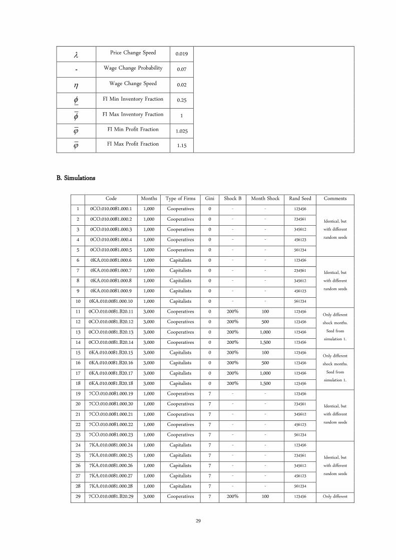
29

Price Change Speed 0.019

- Wage Change Probability 0.07

Wage Change Speed 0.02

FI Min Inventory Fraction 0.25

FI Max Inventory Fraction 1

FI Min Profit Fraction 1.025

FI Max Profit Fraction 1.15

B. Simulations

Code Months Type of Firms Gini Shock B Month Shock Rand Seed Comments 1 0CO.010.0081.000.1 1,000 Cooperatives 0 - - 123456

Identical, but with different random seeds

2 0CO.010.0081.000.2 1,000 Cooperatives 0 - - 234561

3 0CO.010.0081.000.3 1,000 Cooperatives 0 - - 345612

4 0CO.010.0081.000.4 1,000 Cooperatives 0 - - 456123

5 0CO.010.0081.000.5 1,000 Cooperatives 0 - - 561234

6 0KA.010.0081.000.6 1,000 Capitalists 0 - - 123456


7 0KA.010.0081.000.7 1,000 Capitalists 0 - - 234561

8 0KA.010.0081.000.8 1,000 Capitalists 0 - - 345612

9 0KA.010.0081.000.9 1,000 Capitalists 0 - - 456123

10 0KA.010.0081.000.10 1,000 Capitalists 0 - - 561234

11 0CO.010.0081.B20.11 3,000 Cooperatives 0 200% 100 123456 Only different shock months.

Seed from simulation 1.

12 0CO.010.0081.B20.12 3,000 Cooperatives 0 200% 500 123456

13 0CO.010.0081.B20.13 3,000 Cooperatives 0 200% 1,000 123456


15 0KA.010.0081.B20.15 3,000 Capitalists 0 200% 100 123456 Only different shock months.

Seed from simulation 1.

16 0KA.010.0081.B20.16 3,000 Capitalists 0 200% 500 123456

17 0KA.010.0081.B20.17 3,000 Capitalists 0 200% 1,000 123456

18 0KA.010.0081.B20.18 3,000 Capitalists 0 200% 1,500 123456

19 7CO.010.0081.000.19 1,000 Cooperatives 7 - - 123456


20 7CO.010.0081.000.20 1,000 Cooperatives 7 - - 234561

21 7CO.010.0081.000.21 1,000 Cooperatives 7 - - 345612

22 7CO.010.0081.000.22 1,000 Cooperatives 7 - - 456123

23 7CO.010.0081.000.23 1,000 Cooperatives 7 - - 561234

24 7KA.010.0081.000.24 1,000 Capitalists 7 - - 123456


25 7KA.010.0081.000.25 1,000 Capitalists 7 - - 234561

26 7KA.010.0081.000.26 1,000 Capitalists 7 - - 345612

27 7KA.010.0081.000.27 1,000 Capitalists 7 - - 456123

28 7KA.010.0081.000.28 1,000 Capitalists 7 - - 561234

29 7CO.010.0081.B20.29 3,000 Cooperatives 7 200% 100 123456 Only different

30

30 7CO.010.0081.B20.30 3,000 Cooperatives 7 200% 500 123456 months. Seed from simulation 1

and 6 31 7CO.010.0081.B20.31 3,000 Cooperatives 7 200% 1,000 123456


33 7KA.010.0081.B20.33 3,000 Capitalists 7 200% 100 123456 Only different months. Seed

from simulation 1 and 6

34 7KA.010.0081.B20.34 3,000 Capitalists 7 200% 500 123456

35 7KA.010.0081.B20.35 3,000 Capitalists 7 200% 1,000 123456

36 7KA.010.0081.B20.36 3,000 Capitalists 7 200% 1,500 123456

31

Appendix C: Code

Main.java Simulation.java

Agents.java Household.java

FirmB.java FirmC.java FirmE.java

Io.java

(on attached file)

Agent Based Modelling

Documents

Transcript of Agent Based Modelling