Agent-based Computational Transaction Cost Economics

Agent-based Computational

Transaction Cost Economics

Publisher: Labyrint Publication

P.O. Box 662

2900 AR Capelle a/d IJssel

The Netherlands

Fax: +31(0)10 284 7382

Printed by: Ridderprint, Ridderkerk

ISBN 90-72591-79-8

Copyright c 2000 by Tomas B. Klos

All rights reserved. No part of this publication may be reproduced, stored

in a retrieval system of any nature, or transmitted in any form or by

any means, electronic, mechanical, now known or hereafter invented,

including photocopying or recording, without prior written permission of

the copyright owner.

Rijksuniversiteit Groningen

Agent-based Computational


Proefschrift

ter verkrijging van het doctoraat in de

Bedrijfskunde

aan de Rijksuniversiteit Groningen

op gezag van de

Rector Magni�cus, dr. D.F.J. Bosscher,

in het openbaar te verdedigen op

donderdag 6 juli 2000

om 16.00 uur

door

Tomas Benjamin Klos

geboren op 25 augustus 1970

te Apeldoorn

Promotores:

Prof. dr. B. Nooteboom

Prof. dr. R.J. Jorna

Beoordelingscommissie:

Prof. dr. H.W.M. Gazendam

Prof. dr. N.G. Noorderhaven

Prof. dr. A. van Witteloostuijn

Aan Marlies

Contents

Preface ix

Introduction 1

Motivation . . . . . . . . . . . . . . . . . . . . . . . . . . . . . 3

Organization of the Book . . . . . . . . . . . . . . . . . . . . 4

1 Theoretical Background 7

1.1 Transaction Cost Economics . . . . . . . . . . . . . . . . 8

1.1.1 Behavioral Assumptions . . . . . . . . . . . . . . 11

1.1.2 Characteristics of Transactions . . . . . . . . . . 12

1.1.3 The Argument . . . . . . . . . . . . . . . . . . . 15

1.2 Extensions . . . . . . . . . . . . . . . . . . . . . . . . . . 17

1.2.1 Trust . . . . . . . . . . . . . . . . . . . . . . . . . 17

1.2.2 Matching . . . . . . . . . . . . . . . . . . . . . . 20

2 An Agent-based Approach 23

2.1 Optimization . . . . . . . . . . . . . . . . . . . . . . . . 23

2.1.1 Economic Natural Selection . . . . . . . . . . . . 24

2.1.2 Objections against Optimization . . . . . . . . . . 25

2.2 Agent-based Computational Economics . . . . . . . . . . 35

2.2.1 Complex Adaptive Systems . . . . . . . . . . . . 38

2.2.2 Agent-based Computational

Transaction Cost Economics . . . . . . . . . . . . 39

i

ii CONTENTS

3 The Simulation Model 41

3.1 The Main Loop . . . . . . . . . . . . . . . . . . . . . . . 41

3.2 Preferences: Pro�t, Trust and Loyalty . . . . . . . . . . . 43

3.2.1 Scores and Loyalty . . . . . . . . . . . . . . . . . 44

3.2.2 Pro�tability . . . . . . . . . . . . . . . . . . . . . 46

3.2.3 Trust and Opportunism . . . . . . . . . . . . . . 52

3.3 Matching . . . . . . . . . . . . . . . . . . . . . . . . . . 53

3.3.1 The DCR Algorithm . . . . . . . . . . . . . . . . 55

3.3.2 An Example Application . . . . . . . . . . . . . . 56

3.3.3 Matching Buyers and Suppliers . . . . . . . . . . 57

3.4 Adaptation . . . . . . . . . . . . . . . . . . . . . . . . . 59

3.4.1 Choosing � and � . . . . . . . . . . . . . . . . . . 59

3.4.2 Updating . . . . . . . . . . . . . . . . . . . . . . 60

3.5 Summary . . . . . . . . . . . . . . . . . . . . . . . . . . 61

4 Results 65

4.1 Priming the Model . . . . . . . . . . . . . . . . . . . . . 66

4.2 Adaptive Economic Organization . . . . . . . . . . . . . 70

4.3 Optimal Outcomes? . . . . . . . . . . . . . . . . . . . . . 74

4.4 Adaptive Agents . . . . . . . . . . . . . . . . . . . . . . 78

4.5 Alternative Initialization . . . . . . . . . . . . . . . . . . 82

5 Discussion 85

5.1 Conclusions . . . . . . . . . . . . . . . . . . . . . . . . . 85

5.2 Discussion . . . . . . . . . . . . . . . . . . . . . . . . . . 86

5.3 Further Research . . . . . . . . . . . . . . . . . . . . . . 88

Appendices 91

A Genetic Algorithms 91

B The Simulation Program 93

B.1 Agent-Based, Object-Oriented Programming . . . . . . . 93

B.2 Speci�cation . . . . . . . . . . . . . . . . . . . . . . . . . 94

CONTENTS iii

C Parameters and Variables 103

Bibliography 105

Summary 113

Samenvatting (Summary in Dutch) 119

iv CONTENTS

List of Figures

1.1 E�cient boundary (adapted from: Williamson 1981a) . . 9

2.1 Outcomes in Miller's (1996) experiment . . . . . . . . . . 30

2.2 Tit-for-tat as a Moore machine . . . . . . . . . . . . . . 31

3.1 Buyers are assigned to suppliers or to themselves . . . . 43

3.2 E�ciency due to scale and experience . . . . . . . . . . . 51

3.3 Flowchart of the simulation . . . . . . . . . . . . . . . . 63

4.1 Initial score-di�erentials . . . . . . . . . . . . . . . . . . 72

4.2 Proportion `made' (as opposed to `bought') . . . . . . . . 73

4.3 Buyers' pro�ts . . . . . . . . . . . . . . . . . . . . . . . . 75

4.4 Buyers' normalized pro�ts . . . . . . . . . . . . . . . . . 76

4.5 Buyers' normalized pro�ts in 25 individual runs . . . . . 77

4.6 The 12 buyers' adaptive learning in the space of � and � 79

4.7 The 12 buyers' normalized pro�ts and weighted average � 80

4.8 Buyers' adaptive learning in the space of � and � . . . . 81

4.9 Di�erent ways of initializing strengths . . . . . . . . . . . 82

4.10 Buyers' adaptive learning from various initial positions . 83

v

vi LIST OF FIGURES

List of Tables

1.1 Governance strucures and transactions . . . . . . . . . . 16

2.1 The Prisoner's Dilemma . . . . . . . . . . . . . . . . . . 28

3.1 Example preference-rankings . . . . . . . . . . . . . . . . 56

4.1 Parameters and variables used in the simulation . . . . . 68

4.2 Initial score-di�erentials . . . . . . . . . . . . . . . . . . 71

C.1 Parameters and variables allowed in the simulation . . . 103

vii

viii LIST OF TABLES

Preface

At this point, I would like to thank a number of people who have worked

with me on this thesis in one way or another. First of all, I want to thank

Bart Nooteboom and Ren�e Jorna. Bart saw the potential of Agent-

based Computational Transaction Cost Economics long before it was

called that. I am grateful for his trust in my competence to carry out

this project, which was sometimes even greater than my own. Working

with him is so stimulating that the thought of doing that more often is

almost enough to make me return to the academic world. As a cognitive

psychologist, Ren�e's background is rather di�erent than Bart's as an

economist and mathematician; together they have made things really

di�cult|I mean interesting|for me; Ren�e's complementary perspective

has been most valuable for me and for the project, and I thank him

for his contributions. It consider it an important achievement that this

thesis satis�es them both|a tangible result of our collaboration.

I want to thank Rob Vossen for all his contributions. It has always

amazed me how he was able to give insightful comments and suggestions

on topics I did not think he was familiar with. He also never got tired

of supplying me with the necessary diversion. I also thank him and Bob

Blaauw for being my `paranymphs'. I would also like to thank Henk

Gazendam, Niels Noorderhaven and Arjen van Witteloostuijn for their

e�orts as members of the dissertation committee and for the just-in-time

delivery of their comments.

There have been many colleagues at the faculty of Management and

Organization and various other faculties of the University of Groningen,

who have contributed to my undertaking in various ways. In particular|

ix

x PREFACE

and in alphabetical order|I would like to mention Maryse Brand, Hans

van den Broek, Gerda Gemser, Constantijn Heesen, Vincent Homburg,

Gjalt de Jong, Fieke van der Lecq, Delano Maccow, Han Numan, G�abor

P�eli, Wouter van Rossum, Michel Wedel, Wout van Wezel and Frans

Willekens. Outside the University of Groningen, I have enjoyed and

bene�ted from my contacts with Han La Poutr�e and David van Bragt

at the Center for Mathematics and Computer Science in Amsterdam.

Outside the Netherlands, Leigh Tesfatsion at Iowa State University and

Kathleen Carley and John Miller at Carnegie Mellon University have

been very helpful. I also want to thank Christina Dorfhuber and Curt

Topper for putting me up (and putting up with me) during my visit to

Carnegie Mellon University.

I am grateful to the Dutch Organization for Scienti�c Research (NWO),

the Graduate School and Research Institute SOM, the Interuniversity

Center on Social Science Theory and Methodology (ICS), and the Santa

Fe Institute for their generous �nancial support that made it possible

for me to attend various conferences and undertake several other trav-

els and activities. I want to thank colleagues at those conferences, and

especially the class of '97 of the Santa Fe Institute Summer School on

Computational Economics.

Finally, I owe so much to Marlies that I �nd it hard to express this in

words. I hope that dedicating this book to her makes it clear how much

she means to me.

Tomas Klos

Groningen, May 2000

Introduction

\It is the process of becoming

rather than the never-reached end points

that we must study if we are to gain insight."

(Holland 1992, p. 19)

This thesis deals with processes and outcomes of organizing, building on

an economic organization theory, transaction cost economics. Organiz-

ing refers to the adoption of structural forms for coordinating activities:

how are activities distributed and coordinated within and between �rms?

Which �rms perform which activities and how are the interfaces between

them organized? Transaction cost economics is an economic theory that

analyzes outcomes of organizing directly: which organizational forms are

the most appropriate, i.e. `economic', under given circumstances? The

hypothesis is that these are also the forms to be found in reality because

�rms not using these forms will not survive and will be forced to switch

to the appropriate ones. In this thesis, a variety of arguments against

this assumption are brought forward and a di�erent approach is used to

come up with statements about the organizational forms to be found in

reality. Focusing on the process of organizing|and on outcomes only

indirectly|this thesis develops a theory of `adaptive economic organi-

zation'. Rather than from a rational analysis of which organizational

forms are most appropriate for organizing di�erent types of transactions,

statements are derived from computer simulations of the process in which

�rms adaptively learn to organize transactions.

Transaction cost economics (Coase 1937, Williamson 1985) is con-

cerned with the organization of `transactions' of goods or services be-

1

2 INTRODUCTION

tween stages of activity, and yields propositions about which organiza-

tional forms are appropriate for which types of transactions. Simply put,

two consecutive stages might be brought together within a single �rm,

using hierarchy to organize transactions between the stages; or the di�er-

ent stages could be distributed across separate, specialized �rms, using

the market to organize transactions between them. In the �rst case, the

bene�ts from trade (specialization, economies of scale) are not fully ex-

ploited, but the coordination of the transaction is easier and therefore

less costly, because both sides of the transaction fall under the supervi-

sion of a common superior, who can design and impose the terms of the

transaction in a way that is optimal for the �rm as a whole. In the sec-

ond case, the parties on both sides of the transaction are specialized �rms

who may produce more economically, but they are also autonomous and

may have con icting interests, so that the terms of trade will be costly

rather than easy to design and enforce in their mutual interest.

According to transaction cost economics (henceforth TCE), the deci-

sion between these alternatives is made by `aligning' organizational form

(`governance') with the attributes of the transaction to be organized in

such a way that the total of production and organization costs is min-

imized, i.e. in an economic way. Given the characteristics of a trans-

action, certain organizational forms are more appropriate for organizing

the transaction, in that they lead to lower total costs. The theory hy-

pothesizes that the most appropriate organizational form will be used

for organizing the transaction. It also assumes that individual economic

agents are boundedly rational as well as potentially opportunistic. The

�rst of these two behavioral assumptions means that it is very hard|if

not impossible|to design the terms of a transaction between autonomous

contracting parties in such a way that all possible future contingencies

are covered. First of all, not all information about events in the future

is available and secondly, were that information available, it is typically

still impossible, due to limited capacity for processing information, to

perform the task of designing an appropriate contract that prescribes

optimal actions to be taken in the event of each contingency. The con-

dition of bounded rationality could be a problem because of the second

assumption (that people are potentially opportunistic), which says that

MOTIVATION 3

people pursue their self-interest with guile. People can not be blamed for

pursuing their self-interest, and the fact that they do is not a problem

by itself, if all relevant information|including that obtained from the

contracting partner|can be used to design measures to counter negative

e�ects of the partner's pursuing his self-interest. The fact that people

seek self-interest with guile means that they distort the truth and dis-

guise and withhold facts, which makes designing counter measures more

di�cult and costly, or even impossible.

Motivation

Transaction cost theory contains a rational analysis of which organiza-

tional forms are optimal for di�erent types of transactions, given that

agents are boundedly rational and possibly opportunistic. It is then hy-

pothesized that these optimal organizational forms are the ones to be

found in reality: boundedly rational agents are hypothesized to use or-

ganizational forms that result from a rational analysis, which they are

explicitly assumed to be unable to carry out. The argument underly-

ing this (seemingly?) contradictory hypothesis|as well as many others

in economic science more generally|is that suboptimal organizational

forms are presumed to be selected out by market forces; agents using

them allegedly do not survive this `struggle for pro�t' (Friedman 1953).1

In economics, therefore, it is irrelevant whether or not people are able to

determine what is optimal|their behavior will be consistent with that

anyway, because if it is not, it will not survive. What is relevant, is that

economists themselves are able to determine which behavior is optimal,

because it gives them their hypotheses.

Putting it this bluntly may seem somewhat antagonistic and it is also

not altogether fair. It really does not matter whether hypotheses about

boundedly rational agents are derived from a rational, formal analysis

1This presumption is often illustrated with Friedman's (1953) example of a billiards

player who may never even have heard of the laws of mechanics, but will play as if

he applied them to every shot, because he would never win if he did not play in such

a way.

4 INTRODUCTION

or otherwise. What is at issue here, is whether the `economic natural

selection' argument that relates TCE's rational analysis to its main hy-

pothesis, holds and whether, therefore, TCE's analysis is even relevant

for the study of economic organization. In this thesis, it is suggested that

for a variety of reasons (discussed in more detail in Chapter 2), this is

not the case. Essentially, the market is not completely e�cient as a se-

lection mechanism; an evolutionary selection process does not eliminate

all forms of behavior based on trust and cooperation, like TCE suggests

(Williamson 1985); �nally, an evolutionary selection mechanism is not

even appropriate in the �rst place. As discussed in Chapter 2, there are

several reasons why biological and economic natural selection can not be

compared.

In this thesis, a di�erent approach is therefore proposed to generate

hypotheses about economic organization. This alternative approach is

agent-based: it regards multiple, boundedly rational agents in each oth-

ers' contexts and in principle allows all forms of behavior|suboptimal as

well as optimal (although it really can not be established what optimal

is, once a multitude of co-dependent agents are included in a model).

Reinforcement learning is then attributed to the agents, and the whole

system of agents is simulated on a computer to �nd out which organiza-

tional forms the agents learn to adopt.

Organization of the Book

For this alternative approach, we borrow some elements from transaction

cost economics, but not its analysis. Furthermore, some extensions are

required in order to be able to incorporate the in uence of the other

agents in each individual agent's environment. This is the subject of

Chapter 1 that describes the theoretical background for the research. In

Section 1.1, TCE's behavioral assumptions are discussed along with the

attributes that can be used for describing and classifying transactions.

On the basis of that discussion, although it is not used in this thesis, the

theory's analysis is reproduced for the sake of readers not familiar with

transaction cost economics.Theoretical extensions required to include the

ORGANIZATION OF THE BOOK 5

in uence of agents in the environment are discussed in Section 1.2.

The main deviation from TCE lies in the process-approach that was

taken, as discussed above. This is set out in more detail in Chapter 2.

Rather than focus on the optimal outcomes of transaction cost economic

reasoning and hypothesize that these outcomes are found in reality, the

approach taken in this thesis is to focus on the process of organizing in

order to be able to explain, predict and manage the outcomes that re-

sult from such processes. In Section 2.1, it is explained why (transaction

cost) economics is not able to do this and why we think it is necessary.

Also, a method is proposed that makes possible the study of outcomes

as the result of and in relation to the processes that lead to those out-

comes. Individual, boundedly rational agents (�rms) are confronted with

problems of organization and are not given the apparatus of transaction

cost economic logic to help them solve those problems. Instead, they are

assumed (and therefore enabled) to organize adaptively, in a process of

learning which organizational forms work well and which do not. This

may or may not lead to their adopting transaction cost economic organi-

zational forms|although the process is, in principle, not even assumed or

required to ever settle down to a stable state in the �rst place|just like

�rms in reality rarely `align perfectly'. Instead of searching for outcomes

that �rms may never use, therefore, for a variety of reasons discussed in

the chapter, we propose to use computer simulations to model and repro-

duce the process by which agents adaptively search for satis�cing|rather

than optimal|organizational forms, to generate alternative hypotheses

about which forms economic agents (come to) use.

The computer simulation model that is used is presented in Chap-

ter 3. It includes a number of buyers and suppliers who interact with

each other in a number of timesteps. In each timestep, the buyers are

faced with the problem of organizing a particular transaction. They

may organize it within their own �rm, or in a relation with a supplier.

All agents' choices together determine the `payo�' that each of them re-

ceives. In subsequent timesteps, choices that yielded higher payo�s are

more likely to be made again, while choices that returned lower payo�s

are likely to be abandonded. The simulation model is described at a

relatively abstract, implementation-independent level; the details of the

6 INTRODUCTION

actual implementation are described in Appendix B.

The results of experiments with the simulation model are presented

and discussed in Chapter 4. A number of variables in the model were

varied and the e�ect on the outcomes of the simulation are analyzed and

discussed. Overall conclusions are drawn and discussed in Chapter 5,

along with limitations of the current approach and suggestions for further

research.

Chapter 1

Theoretical Background

This chapter presents the theoretical background for the thesis. This the-

ory deals with the organization of transactions that occur between suc-

cessive stages of activity. For example, components have to be brought

from where they are produced to where they are assembled into a �n-

ished product, iron ore or coal has to be transported from the mine to the

smelter to the steel producer, and knowledge has to be transported from

where it is created (using money) to where it is used (to make money).

The phrase `successive', by the way, is not used to suggest that only

vertical relations are implied, but simply that one activity happens be-

fore another; these may be di�erent activities at the same level between

di�erent �rms (in cooperative R&D, for example), yielding a horizontal

relation.

In any case, goods and services have to be transferred from one stage

to another. The main substantive theory used here is transaction cost

economics, which says what the best structural form is for organizing

such transfers. For example, both stages might be brought together

within the bounds of a single �rm|i.e. vertically integrated|or put in

separate �rms, using the market to organize transactions between them.

A company might own its own R&D department, or outsource research

work to a specialized institute. Depending on the characteristics of the

transaction, some organizational forms are more appropriate than others.

Transaction cost economics is about �nding the most appropriate|i.e.

7

8 CHAPTER 1. THEORETICAL BACKGROUND

the economic|organizational form for a given transaction.

Transaction cost theory is described in Section 1.1. The approach

used in this thesis requires certain substantive extensions, described in

Section 1.2. These will be shown to supplement transaction cost eco-

nomics in a very natural way. Methodological issues, on the other hand,

are discussed in Chapter 2, where objections are raised to the approach

taken in TCE, and where the alternative approach that was taken in this

research is presented.

1.1 Transaction Cost Economics

Transaction cost economics says which structural form should be used

for organizing a given transaction. \A transaction occurs when a good

or service is transferred across a technologically separable interface. One

stage of activity terminates and another begins" (Williamson 1981a, p.

552). Rather than focus on individual stages of activity|viewing the �rm

as a production function to be optimized|TCE focuses on transactions

between stages of activity and views the �rm as one of the organizational

forms that may be used to organize such transactions.

Figure 1.1 shows an example. The �gure shows a �rm whose techno-

logical core consists of three stages of production, S1, S2, and S3. These

are the �rm's core activities and|in the example|it `always' performs

those itself. Raw materials production is R, which, likewise, the �rm has

decided `never' to perform itself, and distribution of �nished products is

D. This is not to say that the �rm will indeed always perform each of the

productive stages Sx itself, but it will in the context of the example, in

which this is not at issue. More generally, all such decisions about which

activities a �rm performs will eventually have to be justi�ed in terms of

transaction cost economic reasoning.

Each stage of production Sx uses a component Cx, which has to be

produced. The choice exists for the �rm to produce the component itself

(Cx-M for make) or to let a specialized outside supplier produce it (Cx-B

for buy). The same applies to distribution D, which is D-M if the �rm

owns distribution and D-B if the �rm uses market distribution. Each of

1.1. TRANSACTION COST ECONOMICS 9

C1-M C2-M C3-MD-M

R S1 S2 S3

C1-B C2-B C3-BD-B

potential transactionactual transaction

Figure 1.1: E�cient boundary (adapted from: Williamson 1981a).

the four transactions Cx{Sx (x = 1; 2; 3) and S3{D might be organized

within, as well as across the �rm's boundary, which is the thick black

line. In this particular case, the decision has been made to make C2

and to also keep distribution in-house, and to buy components C1 and

C3. Transactions C2{S2 and S3{D-M, therefore, are organized within

the �rm's boundary, while transactions C1{S1 and C3{S3 are organized

across the �rm's boundary, i.e. on the market.

Transaction cost economics is a theory about this mapping of orga-

nizational forms onto transactions. TCE originated in Coase's (1937)

paper The Nature of the Firm, in which he set out \to discover why a

�rm emerges at all in a specialised exchange economy" (Coase 1937, p.

390); in other words, \in view of the fact that it is usually argued that co-

ordination will be done by the price mechanism, why is such organisation

necessary?" (1937, p. 388). Coase based his answer on the recognition

that the transaction should be the unit of analysis and that �rms and

markets are alternative organizational forms that can both be used for

organizing a transaction. According to Coase, then, �rms exist because

there are costs of using the price mechanism that market-organization


relies on.1

Transacting on the market requires, for instance, that prices are es-

tablished and that contracts are designed. Some or all of these costs

can be reduced or even eliminated when �rm- is substituted for market-

organization. Instead of having to conclude a separate contract for each

transaction to tell the parties involved what to do under which circum-

stances, both parties agree to obey the directions of an entrepreneur

or hierarchichally superior manager, who decides on those directions in

the interests of the �rm as a whole. Were the parties separate and au-

tonomous, each would want to decide on the various terms of the contract

in his own interests. The resulting costs of negotiating (`haggling') and

designing contracts in this manner are transaction costs and some of

them can be avoided by using �rm-organization. This is how di�erent

organizational forms in uence transaction costs, so the question \why

co-ordination is the work of the price mechanism in one case and of the

entrepreneur in another" (Coase 1937, p. 389) can be explained by re-

lating characteristics of transactions to the costs of those transactions

when organized using each possible organizational form. For di�erent

transactions, di�erent organizational forms will best be able to econo-

mize on those costs, which is why organization will be the work of the

price mechanism in one case and of the entrepreneur in the other.

Coase's work was carried further|among others2 and mainly|by

Williamson (1975, 1985), who gives a thorough analysis of the character-

istics of transactions and of the way they in uence the abilities of di�erent

organizational forms to economize on the costs of transactions. Further-

more, Williamson included the e�ects of the characteristics of human

decision makers within organizations on ex post transaction costs, next

to the ex ante transaction costs that Coase (1937) focused on. Ex ante

1Coase received the 1991 Nobel Prize in Economics \for his discovery and clari�-

cation of the signi�cance of transaction costs and property rights for the institutional

structure and functioning of the economy" (quoted from the website of the Nobel

foundation at http://www.nobel.se/).2Olson (1965, p. 12), for example, also writes about \economic organizations that

are mainly means through which individuals attempt to obtain the same things they

obtain through their activities on the market".


transaction costs are the costs that have to be incurred before a trans-

action can occur; partners have to search and �nd each other, and they

have to negotiate a contract. Ex post transaction costs are the costs that

have to be incurred once the transaction is underway and the agents have

committed themselves to it; they have to monitor the partner to ensure

that he keeps up his end of the bargain and respond to unforeseen cir-

cumstances that may arise. What follows is a description of transaction

cost analysis that is based mainly on the writings of Williamson. Sec-

tion 1.1.1 discusses behavioral assumptions, Section 1.1.2 characteristics

of transactions, and Section 1.1.3 outlines transaction cost economics'

main argument.

1.1.1 Behavioral Assumptions

Decision makers' characteristics are summed up in the two `behavioral

assumptions' that|in Williamson's rendering|underlie transaction cost

economics, namely that agents are boundedly rational as well as poten-

tially opportunistic.3 Bounded rationality refers to the fact that people

(agents) are intendedly rational, but only limitedly so. So although eco-

nomic agents may want to choose optimally, they are typically unable

to gather as well as process all the information required to make such

decisions. Information about future circumstances will always be incom-

plete and the agent's cognitive architecture is limited in various ways.

Moreover, certain classes of decision making problems themselves can be

proven to be insoluble|even with unlimited processing capacity. Think

3The term `agent' is used to refer to economic entities|people as well as �rms. A

�rm's `behavior', like decision making, is considered to be a function of the behav-

ior of the human agents within the �rm; those individuals' personal characteristics,

like trustworthiness and general attitude towards the world, a�ect the resulting �rm

behavior|Ring and van de Ven (1994) make the distinction between characteristics

of decision makers `qua persona' and `qua organizational role'. Although we ab-

stract away from the actual individuals within the �rm and also from the politics of

intra-organizational decision making, we do let certain personal traits re-emerge at

the �rm-level, as the outcome of some kind of|not explicitly modeled|aggregation

across all of the �rm's constituents. See (Masuch and LaPotin 1989) for a model in

which this micro-macro link is modeled explicitly.


of the game of chess for an example. These are some of the consider-

ations that underly the assumption of bounded rationality; a complete

treatment of the issue is beyond the scope of this thesis.

Opportunism is self-interest seeking with guile. This goes beyond

simple self-interest seeking to include \calculated e�orts to mislead, dis-

tort, disguise, obfuscate, or otherwise confuse" (Williamson 1985, p. 47).

It is not assumed that every agent is opportunistic all the time, or that

all agents are opportunistic in the same degree; just that some are more

prone to opportunism than others, and that this is impossible, with cer-

tainty, to judge ex ante. Opportunism will be discussed in more detail

and in relation to trust in Section 1.2.1.

Bounded rationality implies (ex ante) incomplete contracting and po-

tential opportunism implies (ex post) moral hazard. Were rationality

unbounded, then it would not matter that agents could possibly act op-

portunistically, because any circumstance in which they would, could be

dealt with in the (comprehensive) contract. If, alternatively, there were

no opportunism, then it would not matter which circumstances would

occur, because they would always be responded to in an honest and co-

operative manner. Real contracting problems only occur, therefore, when

bounded rationality and the possibility of opportunism are both allowed

for, which TCE does.

1.1.2 Characteristics of Transactions

The dimensions relevant for describing and classifying transactions are

uncertainty, frequency and|most importantly|asset speci�city. The

analysis of the role of asset speci�city is one of Williamson's (and TCE's)

main contributions to the study of economic organization (Williamson

1971, Klein et al. 1978); it will therefore be discussed �rst.

Asset speci�city

Asset speci�city refers to the specialization to a transaction of assets that

were invested in to support it. To the extent that assets are speci�c to a

transaction, sustaining the transaction during the period in which returns


on the investments are generated, is a necessary condition for generating

those returns. An example is the construction of an iron-ore smelter near

a steel production plant. The advantage of locating the smelter near the

plant is that the molten iron can quickly be transported to the steel

mill without having to be re-heated. The value of the smelter in this

sense, however, is much lower for other transactions, i.e. transactions

between the smelter and any other steel mill located farther away. In

order to obtain returns on the investment in the smelter, therefore, the

transaction with this particular steel mill has to continue for a particular

period of time, and the investor in the smelter will want to set up a

contract to guarantee the sale of enough molten iron during that period,

so as to generate su�cient returns on his investment in the smelter. The

dependence, however, works both ways, since the steel producer will want

to guarantee the delivery of molten iron that he does not have to re-heat

himself.

Another often-used example concerns the mould that a car-door man-

ufacturer has to invest in to support his transaction with a car producer

for whom he produces doors. The mould can only be used to produce

car-doors for the cars that this particular car manufacturer produces, so

the transaction between these two parties has to exist for as long as the

car-door manufacturer needs, to generate the required returns on his in-

vestment in the mould. If the relation breaks prematurely, however, the

car manufacturer will also experience problems in the supply of car-doors

for his particular model.

Specialized assets allow products to be di�erentiated and pro�t mar-

gins to be increased (this is dealt with in more detail in Chapter 3).

Specialized assets also generate production cost savings as compared to

the use of `general purpose' assets (a smelter located nowhere near the

steel mill). Beside these positive e�ects on costs and returns, what is

important about asset speci�city, is the limited ability to redeploy such

specialized assets outside the transaction in which they were invested,

should the contract execution period be interrupted or terminated pre-

maturely. This poses the dilemma that savings may result from invest-

ments in transaction speci�c, rather than general purpose assets, while

costs have to be spent on a contract, to protect the period required for


generating returns on the investments, from ending prematurely as a re-

sult of the partner's opportunism. Transaction speci�c assets e�ectively

lock the parties involved in an exchange into one another, and give them

a rationale for investing in (the governance of) the transaction itself, so as

to guarantee the successful completion of the contract, lest investments

in specialized assets be lost.

Uncertainty

Uncertainty can be exogenous or endogenous. Exogenous uncertainty

refers to the possiblity that circumstances arise during the contract ex-

ecution phase, that were not foreseen at the moment the contract was

drawn up, and to which the parties will therefore have to adapt the con-

tract. This is where endogenous or behavioral uncertainty comes into

play, which has to do with the fact that, at such moments, the partner

may behave opportunistically.

The relevance of uncertainty is that if there is much uncertainty, there

are many situations that may occur and that would require the partners

involved in a transaction to adapt to. This is very expensive, and there

are also many opportunities for agents to behave opportunistically. In

principle, the higher the uncertainty surrounding the transaction, the

more appropriate it is to organize the transaction internally rather than

on the market. Within the organization, uncertainty can more easily be

reduced, since authority can be used to exercise control over the activities

of di�erent agents within the organization. When di�erent �rms are

involved, it is much harder to guarantee that the di�erent sides of the

transaction live up to their end of the contract.

Frequency

As Coase (1937) already noted, the frequency with which a transaction

occurs matters. If a transaction occurs very often, it may be worthwhile

to establish a specialized organizational form (i.e. a �rm) in which to

organize it, so as to economize on the costs of concluding separate con-

tracts for each transaction on the market. If a transaction only occurs


rarely, it is probably best to organize that transaction with another �rm,

because otherwise the other end of the transaction would also have to be

organized within the �rm. Such investments can simply not be recouped

when they are only used infrequently.

1.1.3 The Argument

According to Williamson, \the central problem of economic organization"

(Williamson 1996, p. 153) is adaptation: of governance to transactions.

Transaction cost economics relates governance forms to transactions in

a discriminating|mainly transaction cost economizing|way. The econ-

omizing capabilities of di�erent forms of governance depend on the at-

tributes of transactions described above, given that agents are boundedly

rational and potentially opportunistic. TCE looks mainly at transaction

costs, but in general, the trade-o� should be considered between costs of

governance (transacting and organizing) and of production: \[a] trade-

o� framework is needed to examine the production cost and governance

cost rami�cations of alternative modes of organization simultaneously"

(Williamson 1985, p. 61).

Because of the �rst of TCE's two behavioral assumptions|that agents

are boundedly rational|contracts are necessarily incomplete, so that

before the end of the period during which the transaction needs to be

sustained in order to gain returns on investments in speci�c assets (if

any), unforeseen contingencies may arise to which the parties will have

to adapt. However, when separate, autonomous �rms are involved, then

because of TCE's second behavioral assumption|that agents are poten-

tially opportunistic|this adaptation can not be assumed to be coopera-

tive (i.e. in their mutual interest), but will rather result in costly haggling

over the distribution of the unforeseen gains or losses (Williamson 1981a).

If no speci�c assets have been invested in, then both parties can go their

own way, but if transaction-speci�c assets have been invested in, then

organizing the transaction between separate, autonomous, potentially

opportunistic �rms, will lead to costs of safeguarding returns on those

investments. If those costs become too high, because assets are very

speci�c, then organizing the transaction within a single �rm's hierarchy


economizes on those costs, because in that case, both parties belong to

the same �rm and will be more likely to have the same interests (those

of the �rm); otherwise, a (hierarchichally superior) manager will decide

in the best interest of the �rm.

This reasoning lead Williamson (1979) to the mapping depicted in

Table 1.1. If assets are not speci�c, then they can easily be redeployed in

Investment CharacteristicsNonspecific Mixed Idiosyncratic

Occ

asio

nal

MarketGovernance

Trilateral(Neoclassical

GovernanceContracting)

Fre

que

ncy

Re

curr

en

t (ClassicalContracting) Bilateral

Governance(Relational

UnifiedGovernance

Contracting)

Table 1.1: Matching governance strucures with commercial transactions

(adapted from: Williamson 1979).

another transaction. There is no need for specialized governance struc-

tures in this case, so, no matter what the frequency of the transaction, it

can easily be organized on the market. Purchasing standard equipment

or materials are examples of this type of transaction. When assets are

speci�c in a non-trivial degree, there is an interest in seeing the contract

through to completion. When such a transaction occurs only occasion-

ally, setting up a specialized governance is too expensive, so a standard

contract with the possibility of arbitrage by a third party such as a court

should be used. When the transaction occurs frequently, on the other

hand, investments in specialized governance are warranted, in the form

of relational contracting. This can be in the form of bilateral governance

of the transaction when asset speci�city is not too high, but when it is,

the bene�ts of specialization are not high enough to o�set the cost of

bilateral governance, so uni�ed governance should be used in this case.

1.2. EXTENSIONS 17

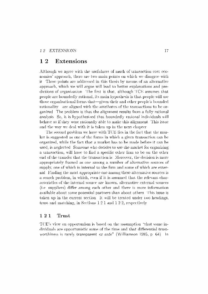
1.2 Extensions

Although we agree with the usefulness of much of transaction cost eco-

nomics' approach, there are two main points on which we disagree with

it. These points are addressed in this thesis by means of an alternative

approach, which we will argue will lead to better explanations and pre-

dictions of organization. The �rst is that, although TCE assumes that

people are boundedly rational, its main hypothesis is that people will use

those organizational forms that|given their and other people's bounded

rationality|are aligned with the attributes of the transactions to be or-

ganized. The problem is that the alignment results from a fully rational

analysis. So, it is hypothesized that boundedly rational individuals will

behave as if they were rationally able to make this alignment. This issue

and the way we deal with it is taken up in the next chapter.

The second problem we have with TCE lies in the fact that the mar-

ket is suggested as one of the forms in which a given transaction can be

organized, while the fact that a market has to be made before it can be

used, is neglected. Someone who decides to use the market for organizing

a transaction, will have to �nd a speci�c other �rm to be on the other

end of the transfer that the transaction is. Moreover, the decision is more

appropriately framed as one among a number of alternative sources of

supply, one of which is internal to the �rm and some of which are exter-

nal. Finding the most appropriate one among these alternative sources is

a search problem, in which, even if it is assumed that the relevant char-

acteristics of the internal source are known, alternative external sources

(i.e. suppliers) di�er among each other and there is more information

available about some potential partners than about others. This issue is

taken up in the current section. It will be treated under two headings,

trust and matching, in Sections 1.2.1 and 1.2.2, respectively.

1.2.1 Trust

TCE's view on opportunism is based on the assumption \that some in-

dividuals are opportunistic some of the time and that di�erential trust-

worthiness is rarely transparent ex ante" (Williamson 1985, p. 64). In


other words, since it is hard to tell who will be opportunistic and when,

the possibility of opportunism is always reckoned with and measures to

counter its e�ects are always necessary.

In regarding opportunism, it is instructive to make the distinction be-

tween room for and inclination towards opportunism (Nooteboom 1999b)

and to consider that actual opportunism is a function of the two. In

TCE, however, information about the potentially opportunistic party's

inclination to behave opportunistically is not allowed to enter the anal-

ysis, simply because that would make it too complex (Williamson 1985,

p. 59):

\[i]nasmuch as a great deal of the relevant information about

trustworthiness or its absence that is generated during the

course of bilateral trading is essentially private information|

in that it cannot be fully communicated to and shared with

others (Williamson 1975, p. 31{37)|knowledge about behav-

ioral uncertainties is very uneven. The organization of eco-

nomic activity is even more complicated as a result."

So, even though it is admitted that relevant information about trustwor-

thiness is generated during the course of bilateral trading|information

agents may use to reduce endogenous uncertainty|this information is

not included in the analysis, because that would make the organization

of economic activity to be explained too complicated. In this thesis, the

suggested increase in the complication of the organization of economic

activity is not admitted as a justi�cation for not addressing it. On the

contrary, it is proposed and subsequently shown that this complication

can be dealt with using the appropriate apparatus. In particular, the con-

sequences of incorporating relevant information about trustworthiness for

the organization of economic activity will be explored by modeling `the

course of bilateral trading' explicitly and at the appropriate level|i.e.,

the level of the individual �rms involved in bilateral trading. This allows

us to incorporate the e�ects of the accumulation and subsequent use of

`relevant information about trustworthiness or its absence'. Furthermore,

even if it is considered impossible to transfer this private knowledge, in-

dividuals will still use this private information about trustworthiness as

1.2. EXTENSIONS 19

input for their own decisions about the `bilateral trading' they are in-

volved in. Obviously, TCE does not go this way because that would

require going down to the level of individual agents and their boundedly

rational processing of the information. In this thesis, we will go that way.

The way in which the accumulation and use of relevant information is

modeled, can be informed by theories of trust. Since \some individuals

are opportunistic some of the time and (. . . ) di�erential trustworthiness

is rarely transparent ex ante" (Williamson 1985, p. 64), an agent's trust-

worthiness is equal to his not behaving opportunistically. In fact, an

agent's trustworthiness is equal to his not wanting to behave opportunis-

tically. This is where the distinction between room for and inclination

towards opportunism (and that between exogenous and endogenous, or

behavioral uncertainty) is relevant. This is also where the distinction

between trust in intention and trust in competence can be explained

(for a good overview of issues related to trust, see Nooteboom's (1999b,

p. 24{35) discussion). In this thesis, we will be concerned only with

trust in intention; agents are always assumed to be able to live up to

other agents' expectations, so the question is always whether the agent

wants to, rather than whether he is able to. If an agent's trustworthi-

ness is equal to his not behaving opportunistically, then another agent's

subjective interpretation of the probability of that trustworthiness, in

turn, is that other agent's trust in the �rst agent; the second agent's

subjective probability that something does not go wrong (Chiles and

McMackin 1996, Dasgupta 1988, Gambetta 1988). It is interesting to see

that transaction cost economics' main propositions correspond closely

to those derived from a theory of trust (Deutsch 1973). In his `trust

problem in an exchange relationship'|modeled as a prisoner's dilemma

(see Section 2.1.2) in which two players have the options to give or to

retain their own item|Deutsch (p. 161) mentions \three fundamental

ways to guarantee that an exchange will be reciprocated: (1) to employ

arrangements that will make for simultaneity of giving and receiving in

the exchange; (2) to use third parties; and (3) to use `hostages' or `de-

posits,' which will enable each person to commit himself to the exchange

and to be convinced that the other person has also committed himself".

The parallel with TCE's governance structures is obvious. To a large


extent, both theories approach the same issues|just from di�erent di-

rections: TCE from the perspective of opportunism and Deutsch (1973)

from the perspective of trust. In this thesis, they are both used in a

complementary fashion.

1.2.2 Matching

The consequence of trust and of the fact that more relevant information

about trustwortiness is generated during the course of some bilateral

trading relations than others, is that agents have di�erential preferences

for relations with di�erent other agents. A convenient way of incorporat-

ing this fact is by using matching models (see (Roth and Sotomayor 1990)

for an excellent introduction to and overview of matching theory). The

seminal paper by Gale and Shapley (1962) uses marriage markets to il-

lustrate the issues.4

Matching models are used to model and analyze situations where

agents have to be assigned to other agents for certain interactions to pro-

ceed. For example, workers prefer working at some �rms rather than at

other �rms, and �rms will prefer some suppliers to others. The fact that

agents will try to in uence the outcome of the eventual assignment, has

an e�ect on the outcome that results, and on its characteristics. This

contrasts with standard economic theory where individual assignments

are either not explicitly modeled but aggregated across, or assumed to

be random or under the control of a central supervising agent (an auc-

tioneer). When allowance is made for the fact that each agent will rather

be involved with certain agents that with others, models can be made

much more realistic, and predictions can be made for situations where

this phenomenon occurs|for which many interesting situations qualify.

To get an idea of the range of possible applications, consider that Roth

(1984) studied matching models of the market where medical students

compete for internships at the best hospitals (and hospitals compete for

the best medical students), Stanley et al. (1994) and Hauk (1997) applied

4Interestingly, the marriage metaphor has also often been used to analyze issues

in relations between �rms (Nooteboom 1999b, appendix 4.1).

1.2. EXTENSIONS 21

Gale and Shapley's (1962) model in studies of the prisoner's dilemma,

Tesfatsion (1997, 2001) has studied trade networks and labor markets,

and Sherstyuk (1998) examines production coalitions between di�eren-

tially skilled agents. Hauk (1997) mentions matching in the context of

search|gathering of information to be used as an input for the matching;

issues of information gathering and adaptive search for trading partners

are also addressed in the context of industrial buying of �sh on the Mar-

seille �sh market by Weisbuch et al. (forthcoming) and by Kirman and

Vriend (2001). This is precisely the context in which a matching model

was used in the current study; the way this was done is described in the

following chapter.

Chapter 2

An Agent-based Approach

This chapter presents our approach to studying problems of economicorganization. Next to the discussion on substantive extensions to TCEin Section 1.2, this entails a second deviation from the transaction costeconomics approach. In short, we take issue with the focus|in economicsin general and in transaction costs economics in particular|on optimaloutcomes. This focus and our objections against it are discussed in thenext section. A more appropriate way of studying economic organizationis presented in Section 2.2.

2.1 Optimization

One of the pillars on which TCE's analysis rests is the assumption thatpeople are boundedly rational (see Section 1.1.1). If this is not assumed,the argument falls apart because complete comprehensive contracting isthen feasible. With the assumption in place, TCE's analysis is aimed at�nding the most appropriate organizational form for each possible typeof transaction, in the sense of being `aligned' with the attributes of thattransaction|as discussed in Section 1.1.3.

However, the theory then goes on to hypothesize that organizationalstructures are aligned with the attributes of transactions. TCE there-fore, suggests a higher level of rationality. On the one hand, people are

23

24 CHAPTER 2. AN AGENT-BASED APPROACH

assumed to be boundedly rational, but on the other hand, they are hy-pothesized to behave they way they would if they were rationally ableto design the governance structures that are most appropriate given thatthey are boundedly rational. In other words, boundedly rational peopleare hypothesized to use precisely those governance forms for organizingtransactions that they would use if they were unboundedly rational inchoosing or designing them.

2.1.1 Economic Natural Selection

When confronted with this contradiction, (transaction cost) economistswill usually admit that people are indeed not fully rational, but they willgo on to suggest that people will behave like they would if they were(Alchian 1950, Enke 1951, Friedman 1953). Full rationality implies theability to determine what|i.c. which organizational form|is optimal,given the circumstances (of bounded rationality, for example). The ar-gument is that since suboptimal behavior and suboptimal organizationalforms do not survive in the selection process of markets, they will notbe found in empirical research. Presumably, this is why it is allowedto hypothesize outcomes in which transactions are perfectly aligned withorganizational forms, while those responsible for the alignment are at thesame time assumed to be largely unable to perform the alignment.

The reason for using this argument is that it allows economists touse mathematics and other formal methods for modeling problems ineconomics and solving them for optimal equilibrium outcomes. Anotherreason is that, looking at it this way, economists do not have to explainwhy economic activity is organized the way it is and how it has come tobe organized that way rather than some other way. As mentioned in theintroduction, it is irrelevant whether or not people are able to determinewhat is best for them; what matters is that economists are able to dothat.

Apparently, this is preferred over taking the assumption of boundedrationality all the way, which e�ectively means allowing for an in�nitearray of outcomes consistent with more or less rational behavior, rang-ing from full rationality to full stupidity, so to speak. This would mean

2.1. OPTIMIZATION 25

that models would be much more complex and di�cult to analyze andthat hypotheses would be much less straightforward to derive from thosemodels. This is obviously a much more di�cult task but, because of theseriousness of the objections discussed below, it is the one that was un-dertaken in the research described in this thesis|not that it was carriedout completely, by the way. Only a small step was taken towards morerealistic models; the decision-making situation is a very simple one. Themain contributions to a more realistic study of economic organization arethat (1) individual, boundedly rational agents are studied in each other'scontext, in which (2) they adaptively learn to make their own decisionswhile (3) in uencing the consequences of each other's decisions.

2.1.2 Objections against Optimization

The evolutionary argument is used by economists to justify their searchfor optimal outcomes, by stating that suboptimal behavior is not rele-vant because it will not survive the selection process on markets. Theeconomic natural selection argument is awed on several accounts. Ourobjections against it are divided in those against the presumed e�ective-ness of the evolutionary selection process on the one hand, and againstthe appropriateness of the evolutionary model on the other hand.

Objections within the Evolutionary Model

First of all, the economic natural selection argument depends on thee�ectivess of markets in terms of weeding out suboptimal behavior. Thereare several reasons why this e�ectiveness may not be as high as it needsto be. If the argument is that it is only the best behavior that survivesin a population, then the �rst and obvious objection is that economicnatural selection does not yield the best conceivable (as resulting from arational analysis), but merely the best present in the population (Winter1964). Which behavior survives depends on the behaviors present in thepopulation to begin with, and not on the analysis. The implication isthat the population of agents itself should be part of the analysis.

A related point is that if the optimal behavior is not present in the


population to begin with, it should be able to enter the population. Entrybarriers may prevent this and thus protect incumbents and not put thepressure on them that forces them to behave in an optimal manner. Zeropro�ts and price that equals marginal costs are only equilibrium outcomesunder free and costless entry, while positive pro�ts are often observed.Entry, however, is only the �rst phase of the general process in whichoptimal behavior enters the population and then spreads through it.

In the second phase, even if the optimum is present in the populationto begin with or is able to enter the population, a mechanism has to be atwork to transfer this optimal behavior from one agent in the populationto the next. In biological evolution, the process of reproduction performsthis task, but do organizations reproduce? It may be argued that anorganization's genetic material is transferred to the organization's de-scendants in the form of organizational memory. Descendants are thenthe same organization at later moments in time. It is, however, hard toimagine how it could be transferred to other organizations, which it needsto if it is ever going to spread throughout the population, which, in turn,it needs to do if hypotheses based on rational analyses are ever to becon�rmed. Especially tacit organizational knowledge is hard to transfer,because it has to be made explicit �rst, or be transferred in imitationwhich requires physical proximity. Why would organizations do that andtransfer the knowledge that makes them successful to competing �rms?Besides, if there is some imitative process at work, then what may beobserved and imitated is behavior, and not necessarily the underlyingknowledge and rules derived from it that make organizations successful.

Another reason why suboptimal behavior may survive, is that it isoften not in direct competition with organizations behaving in a superiormanner. Not all billiards players always win; they are still able to make aliving if they do not always encounter stronger players. Di�erent culturesexist in di�erent parts of the world, where di�erent ways of doing businessexist (de Jong 1999). Because these groups are separated from each othergeologically or otherwise, their di�erences can remain. Globalization andthe internet, however, make competition more international, which putspressure on some regions as di�erent ways of doing business may invadethem. Evolutionary game theory deals with these issues; see (Nooteboom


1997) for an analysis of whether, in these kinds of models, opportunismwill ever go away.

What these objections mean for transaction cost economics is that itsanalysis may not be helpful in designing hypotheses about economic or-ganization. For example, Williamson (1985, p. 64{65) states that \[o]neof the implications of opportunism is that `ideal' cooperative modes ofeconomic organization, by which I mean those where trust and goodintentions are generously imputed to the membership, are very fragile.Such organizations are easily invaded and exploited by agents who donot possess those qualities", which clearly indicates his thinking in termsof an evolutionary model. As a consequence, such `high-minded' orga-nizational forms are immediatedly rendered nonviable. However, if thishypothesis is based on an evolutionary argument, then, as suggested byKoopmans (1957) long ago, its validity should be tested by modeling theevolutionary process explicitly.1 What Koopmans probably did not havein mind, but what is possible today, is to model the evolutionary pro-cess explicitly by simulating it on a computer, using a so-called geneticalgorithm (see Appendix A, and see (Holland 1975) for the original pub-lication and (Goldberg 1989) for a good general introduction). Miller(1996) did just that and found that an evolutionary process does leadto a high level of cooperation and trust in the population, which sup-ports the view that the evolutionary metaphor does not support TCE'shypotheses.

In Section 2.2, an alternative approach is suggested for coming upwith hypotheses about economic organization. This approach does notonly use additional theoretical insights besides TCE, as discussed in Sec-tion 1.2, but it is also not based on an evolutionary metaphor. In thecurrent section, it has been argued that the evolutionary metaphor does

1See Blume and Easley (1998, p. 23), who \view [their] analysis as showing that

Koopmans' cautionary remarks about the use of natural selection as the basis for

pro�t maximization are correct. We show that it is simply not appropriate to argue

for pro�t maximization on the basis of natural selection and then replace natural

selection by pro�t maximization in either static or dynamic equilibrium analysis. It

may be that pro�t maximizing behavior is a useful hypothesis, but the usefulness of

natural selection as a defense of pro�t maximization is very limited".


not support hypotheses consistent with rational optimization. It wouldbe possible to use a genetic algorithm and derive other hypotheses fromthe evolutionary approach, but that is not what is attempted here, be-cause the evolutionary approach itself is considered inappropriate. Thisis discussed in the next section.

Objections against the Evolutionary Model

I have raised these objections earlier (Klos 1997, Klos 1999), in relationto Miller's (1996) experiments mentioned earlier. They will be discussedhere again, to guide the discussion at hand. Miller used a genetic algo-rithm to evolve a population of strategies for playing the repeated pris-oner's dilemma, which is also an often-used model of inter-�rm relations(see, e.g., Axelrod 1984, Hill 1990, Parkhe 1993). The prisoner's dilemma(PD) is a game that models the con ict between individual and collec-tive interest. Two players both have to choose between cooperating ordefecting (acting opportunistically), without knowing the other player'schoice. Both players then receive a payo� that depends on both players'choices. Table 2.1 shows these payo�s, where T stands for the tempta-

Player IIC D

Player ICD

(R;R)(T; S)

(S; T )(P; P )

Table 2.1: Prisoner's Dilemma if T > R > P > S and 2R > T + S (forthe Repeated PD).

tion to defect when the other player cooperates, R stands for the rewarda player receives when he cooperates when the other player also cooper-ates, P stands for the punishment both players receive when they bothdefect and S stands for the sucker's payo� for the player who cooperateswhen the other player defects.

The payo�s show that each player is better o� by defecting irrespec-tive of whether the other player cooperates (because T > R) or defects


(because P > S). If the game is repeated, this grim perspective disap-pears because the possibility then opens up to make game-play reactiveto previous moves, allowing players to punish defection and reward coop-eration in the previous move, for example. This is only the case when thegame is repeated inde�nitively, however, because if the game has a knownnumber of repetitions, backward induction makes defection the optimalchoice in each round. Both players then know that the other player willdefect in the last round, so they will both defect in the last round. Thismakes defection in the second-to-last round the rational choice as well,and so on until the very �rst round. This backward induction argumentdoes not work if the game has an unknown or in�nite number of rounds.

Miller (1996) used a population of 30 strategies and measured eachstrategy's �tness per generation as the average payo� per move (APM)across 150-round repeated PD's against the 30 strategies in the popula-tion (including itself). After this round-robin tournament, the 30 strate-gies were ranked by decreasing �tness. Miller used an elitist scheme inwhich the top 20 strategies proceeded to the next generation unchangedand 10 new strategies were created in each generation, using 2-pointcrossover conditional upon a 60% crossover-probability and bitwise mu-tation on the o�spring conditional upon a 0.5% mutation probability.This means that 5 consecutive times, 2 strategies were selected fromthe entire previous population and, conditional upon a 60% probability,crossed with each other at two loci, after which each bit in each of the tworesulting o�spring was subjected to a 0.5% probability of being ipped(from 0 to 1 or vice versa).

Miller's (1996) experiments were replicated in (Klos 1999),2 and arepresented in Figure 2.1. This �gure shows the proportion of di�erenttypes of outcomes averaged over the 150 rounds of the game and over allthe games in the whole population in each generation and, in addition,over 40 runs of the experiment. It shows that, under selective pressure,it is in fact not the \ `ideal' cooperative modes" that are \easily invadedand exploited by agents who do not possess those qualities" (Williamson

2Because Miller's (1996) experiments were compared to my own experiments in

which I used 36 agents, I replicated Miller's experiments with 36 strategies as well,

with the same relative size of the elite.


0

0.2

0.4

0.6

0.8

1

0 5 10 15 20 25 30 35 40 45 50

prop

ortio

n

generations

CCDD

CD/DC

Figure 2.1: Outcomes in Miller's (1996) experiment.

1985, p. 64{65). Rather, those cooperative modes are the ones thatsurvive in the long run. The (interesting) implications of these resultsfor transaction cost economics are not derived here, but the focus israther on the criticism I have on the evolutionary approach itself (cf.Klos 1999).

The main objection is that a genetic algorithm is essentially an in-strument of optimization. Even though it is not guaranteed to �nd anoptimum, it is the next best thing to optimizing when that is not possibleanalytically because of the complexity of a model. To this end, evolutionas modeled in a GA and implemented, for example, by Miller, operatesat the population level. Candidate solutions are usually represented asstrings, often binary. These can be interpreted as points in a multidi-mensional search space. Miller (1996), for example, represented RPDstrategies as Moore machines|a kind of �nite state machine (FSM)|which he coded as strings of bits. Figure 2.2 shows the famous strategy`tit for tat' as a �nite state machine. This strategy was invented byAnatol Rapoport and made famous in Axelrod's (1984) tournaments. Itcooperates in the �rst round of the game and then mirrors the opponen-


C D

c

d

c d

S

Figure 2.2: Tit-for-tat as a Moore machine.

t's previous move in subsequent rounds. In general, a Moore machineconsists of (1) a set of internal states (the circles in Figure 2.2), one ofwhich is designated to be (2) the starting state (labeled 'S'), (3) an out-put function that maps each internal state onto an output, i.c. a choicebetween the alternative actions C and D (the uppercase characters insidethe circles) and (4) a transition function that maps each internal stateonto a next state (designated by arrows in Figure 2.2) for each of theopponent's possible actions (the lowercase arrow labels). Miller (1996)used machines with a maximum of 16 internal states, which he coded asstrings of 148 bits.3

Each possible strategy can be seen as a point in a 148-dimensionalspace. Each strategy is a solution to the problem of being successfulin a repeated prisoner's dilemma. This success, of course, depends onthe strategy played against, so Miller let the strategies co-evolve, whichmeans that their �tness and therefore chances of survival are determinedin part by the other strategies in the population. This was achieved bycalculating �tness as the average payo� per move in games against allstrategies in the population in the current generation. Fitnesses can bethought of as values on the 149th dimension, as a �tness-landscape onthe original search space.4 The objective is to �nd the 148-dimensionsal

3Because 4 bits can represent 16 di�erent numbers, it takes 4 bits to designate

the starting state. For each of the 16 states, it takes 1 bit to specify the value of the

output function (0 for C and 1 for D) and 4 bits to specify each of the two values of

the transition function (one for the opponent's cooperation and one for his defection).

This means it takes a total of 4 + 9 � 16 = 148 bits.4It is easier to visualize the �tness-landscape as the third dimension on a 2-

dimensional search space. The objective is then to �nd the highest peak in the

�tness-landscape. The point in the 2-dimensional search space corresponding to that


point with the highest �tness. It is obviously a very hard problem todetermine what the best strategy is, and there probably is not even abest strategy for all circumstances, i.e. against all possible opponents. Agenetic algorithm can very well be used for these kinds of problems thatcan not be solved analytically. Instead of trying to optimize an unknown�ness-function, or calculate the �tness of all possible points in the space,in each of a sequence of generations it samples a limited number of so-lutions in the search space in parallel, and uses information about theperformance of those di�erent solutions to direct search towards promis-ing regions of the search space in the next generation, when it exploresthose promising regions further.

The properties that make a GA successful, however, are the very sameproperties that make it inappropriate for modelling individual agents'adaptive behavior. Most importantly, notwithstanding the e�ects of com-munication and reputation, individuals do not have access to informationabout the performance of all the strategies they did not use themselves;they only have access to their own experience for guiding their search,and maybe those of a limited number of other agents, like the ones theyinteract with directly. These objections can be illustrated by consideringwhat a GA-model means when viewed from the perspective of an indi-vidual in the population. Some very strong assumptions are made|alltoo often only unconsciously.5 These assumptions follow from modelling-decisions made to let the GA function e�ciently and e�ectively, but theyare not realistic from the individual agent's perspective.6

peak is the solution to the problem.5See also Vriend's (1998) experiments, who also confronted the results from a

genetic algorithm (which implements what he calls `social learning') with individual

agents' `individual learning'. His conclusions is that the \lesson to draw here is that

the computational modeling choice between individual and social learning algorithms

should be made more carefully, since there may be signi�cant implications for the

outcomes generated" (1998, p. 11, emphasis added).6Whether or not this is a problem, depends on what the GA is used for, of course.

When it is used with the intention to solve a hard problem, then it does not matter

that these assumptions are implausible from the perspective of the members of the

population|which it does when the GA is used as a representation of individual

adaptive learning. One could, out of curiosity for example, use a GA with the intention


1. First of all, all the agents in the population interact with all otheragents in the population, while people typically only interact witha limited number of others, namely those who are physically, cul-turally, emotionally, or otherwise close to them. This was donebecause it directs the GA's search towards strategies that performwell in general, rather than just against a small number of �xedstrategies (as in Axelrod's (1987) experiments, for example), whichthe population would then specialize to.

2. Secondly, and more importantly, the decision to change a strategyis not taken by the agent using the strategy but by the parame-ters that regulate the GA's operation. For example, the 20 topperformers are forced to keep their strategy, and the 10 worst per-formers are forced to change their strategy. Even apart from thespeci�cs of this elitist scheme, the decision to change a strategy issimply not taken by the agent himself, while, reasonably, it shouldbe. Instead, it is taken on the basis of a comparison of the agent'sperformance and all other agents' performance, whereas, in relationto the �rst point, comparison with only those somehow `close' tothe agent would be more appropriate. This mirrors the fact thatthe GA is not about agents but about strategies; the GA searchesfor optimal strategies, irrespective of what agents using strategieswould do.

3. Thirdly, when comparing an agent's performance to other agents'performance, those other agents' experiences in all their games aretaken into account, most of which the agent did not partake in him-self. Experiences are assumed to be transferable from one agent tothe next. This is an important mechanism that makes the GA suc-cessful, but from the perspective of the individual agent, it means

to replace or supplement TCE's rational analysis in a model that can not be solved

analytically, but then it should not be claimed that the outcome of the GA is a good

hypothesis of what people actually do in situations characterized by that model. It

could be used \as a benchmark against which to assess the performance of more

realistically modelled social learning mechanisms" (Tesfatsion 2001, p. ??).


that he not only has access to the experiences of all other agents inthe population, but also that those are relevant to his own situation.

4. Finally, when creating new strategies, old strategies from the wholepopulation are used, while, in relation to the �rst and second pointsabove, any imitative process would more likely be based on thoseclose to the agent. Moreover, the agent would never even be able toperceive other agents' strategies, but only their behavior in mutualgames, as generated by their underlying strategies. Because theGA operates on strategies, this is not a problem; at the level ofthe population of `solutions', all strategies are visible and can bemanipulated in the search for better ones.

In (Klos 1999), these considerations led me to design a di�erent setup formodeling agents' adaptive social behavior, in which all agents are locatedin the cells of a grid, interact only with their immediate neighbors onthe grid and themselves decide on changing their strategy on the basis oftheir own comparison of their own performance with only their immediateneighbors' performance.

Others have also noticed some of these considerations. In anotherapplication of a GA|derived from a follow-up (Stanley et al. 1994) onan early version of Miller's (1996) experiments (Miller 1989)|Tesfatsion(2001, p. ??), for example, notices that

\[a]n important caution is in order here, however. The in-formation that work suppliers and employers are currentlypermitted to have access to in the evolution step is substan-tial: namely, complete knowledge of the collection of strate-gies used by agents of their own type in the previous tradecycle loop, ranked by �tness. The evolution step is thus moreappropriately interpreted as an iterative stochastic search al-gorithm for determining possible strategy con�guration at-tractors than as a social learning mechanism per se. Theresulting welfare outcomes will be used in subsequent workas a benchmark against which to assess the performance ofmore realistically modelled social learning mechanisms."

2.2. AGENT-BASED COMPUTATIONAL ECONOMICS 35

The point is that we are not interested in `strategy con�guration attrac-tors', but in `more realistically modelled social learning mechanisms'. Onthe one hand, what Tesfatsion (2001) and other economists using geneticalgorithms are doing, is going down to the level of individual agents. Iagree that we should do this, even though it makes models much morecomplex, as discussed in Section 2.1.1. But on the other hand, what theyuse genetic algorithms for is to look for equilibria, `strategy con�gura-tion attractors', and optimal outcomes in those more complex modelsonce again, because their models can not be solved analytically. This isprecisely what I have argued earlier that we should not be doing, whichis why, in the next section, I propose a form of learning at the level ofthe individual, analogous to the model in (Klos 1999).

2.2 Agent-based Computational

Economics

The approach taken in this thesis operates at the level of individual,boundedly rational, adaptive agents. They may still search a space ofsolutions like the 148-dimensional space Miller (1996) created, but theydo so by adapting on the basis of their own personal experiences. Anumber of such agents are allowed to interact with each other and adapttheir behavior on the basis of their experiences in those interactions. Thebehavior that emerges from these interactions may not be optimal at thepopulation level, but it will be at the level of the agent, at least to theextent that the agent's bounded rationality lets him establish that.

This approach falls under the heading of `Agent-based ComputationalEconomics' (ACE), \the computational study of economies modelled asevolving systems of autonomous interacting agents" (ACE-website):7

\A central concern of ACE researchers is to understand theapparently spontaneous formation of global regularities ineconomic processes, such as the unplanned coordination of

7http://www.econ.iastate.edu/tesfatsi/ace.htm


trade in decentralized market economies that economists as-sociate with Adam Smith's invisible hand. The challenge is toexplain how these global regularities arise from the bottomup, through the repeated local interactions of autonomousagents channeled through socio-economic institutions, ratherthan from �ctitious top-down coordination mechanisms suchas imposed market clearing constraints or an assumption ofsingle representative agents."

This approach is used more and more often to study problems ineconomics|problems that can not be solved analytically, because thesearch space is too large or because the function to be optimized is un-known.8 The essence of this approach is to model individual agents ex-plicitly and to focus on the process in which they interact with each otherand adapt their behavior on the basis of their experiences in those inter-actions. Economic phenomena can then be studied as the outcomes thatemerge from actual (simulated) interactions between individual, bound-edly rational, adaptive agents. Whether an interaction takes place be-tween any two given agents is left for them to decide. What the agentssubsequently do in that interaction is their own|possibly sub-optimal|decision, that they make on the basis of their locally available, incompleteinformation and as a result of their own (cognitively-limited) processingof that information.

These processes and the outcomes that emerge from them are con-sidered more interesting and useful than equilibria deduced from mod-els employing representative agents, auctioneers or anonymous, randommatching, etc., models that require very limiting assumptions in orderfor formal derivations to go through. As Schelling (1978, p. 26) putsit, \[t]here is nothing particularly attractive about an equilibrium. An

8Examples include the problem of being successful in the repeated prison-

er's dilemma (Klos 1999, Miller 1996, Stanley et al. 1994), in social dilemmas

(Glance and Huberman 1994) as well as on �nal-goods markets (Albin and Foley

1992, Vriend 1995), stock markets (Arthur et al. 1997), industrial markets (P�eli

and Nooteboom 1997), whole-sale markets (Kirman and Vriend 2001, Weisbuch

et al. forthcoming), labor markets (Tesfatsion 2001), and spatial political models

(Kollman et al. 1992, Miller and Stadler 1998).


equilibrium is simply a result. It is what is there after something hassettled down, if something ever does settle down. The idea of equilib-rium is an acknowledgement that there are adjustment processes". Still,even if it is considered interesting to know what the equilibrium in aneconomic system is, then there are still several reasons for taking upalternative lines of inquiry, such as the study of out-of-equilibrium ad-justment processes|for example by means of computer simulations, asin this thesis.

First of all, an equilibrium may be very hard or even impossible to�nd, or `compute' (cf. the work at the UCLA Center for Computable Eco-nomics9). All that is left, then, is to study out-of-equilibrium dynamics.Secondly, there may be very many equilibria so that investigating howthe system evolves may provide information about which of those equilib-ria are more probable, likely or otherwise interesting than others. Thisis what evolutionary game theory is about. Thirdly, and relatedly, asstated by David (1985),10 \it is sometimes not possible to uncover thelogic (or illogic) of the world around us except by understanding howit got that way". Fourthly, it is possible to study equilibria as the re-sult of and in their relation to out-of-equilibrium dynamics. Much ofthe focus on equilibrium in economics has been forced onto economistsby the di�culty of studying anything else|that is, by the absence ofappropriate tools for studying anything other than equilibrium, like themore interesting adjustment processes mentioned by Schelling (1978).Holland (1992) describes how it has recently become possible to studycomplex adaptive systems using computer simulations and states that,now that it's possible, \[i]t is the process of becoming rather than thenever-reached end points that we must study if we are to gain insight"(1992, p. 19). Finally, if one wants to intervene in a process with theintention of reaching a desired outcome, one needs to understand how theprocess that leads to the outcome, does so, and what the e�ects of mea-sures taken now, are on the outcome obtained later (Nooteboom 2000).

9http://cce.sscnet.ucla.edu/10This often-cited paper provides the main example of `path dependence' (the lock-

in to the QWERTY typewriter con�guration), on which much work by Brian Arthur

and others at the Santa Fe Institute (http://www.santafe.edu) is based.


One needs positive knowledge about the way the system develops, whichmight be revealed by computer simulations|or by longitudinal empiricalstudies, but those are often not feasible in studies of managament andorganization. Besides, in empirical research it is impossible to observethe e�ects of measures not taken, while computer simulations can alwaysbe re-run under di�erent settings; these are the traditional advantages ofcomputer simulations. Epstein and Axtell (1996) refer to these arti�cialsocieties using the term `CompuTerrarium', in which social structurescan be grown `in silico'.

2.2.1 Complex Adaptive Systems

ACE is the specialization to economics of the basic Complex AdaptiveSystems (CAS) paradigm. There are two important aspects of CAS.

Complex Systems . . .

A complex adaptive system (CAS) \is a complex system containing adap-tive agents, networked so that the environment of each adaptive agentincludes other agents in the system" (Holland and Miller 1991, p. 365).This paradigm seems to �t very well the case of transaction cost eco-nomics, where, according to a recent statement by the founding father oftransaction cost reasoning, Coase (1995, p. 245)

\[t]he analysis cannot be con�ned to what happens withina single �rm. The costs of coordination within a �rm andthe level of transaction costs that it faces are a�ected by itsability to purchase inputs from other �rms, and their abilityto supply these inputs depends in part on their costs of co-ordination and the level of transaction costs that they facewhich are similarly a�ected by what these are in still other�rms. What we are dealing with is a complex interrelatedstructure."

Holland (1992) and Holland and Miller (1991) suggest to study eco-nomic systems as complex adaptive systems. The CAS approach appears


to be ideally suited to deal with Coase's (1995) observation, which is whatis attempted in the research described in this thesis.

. . . and Adaptive Agents

An agent in a Complex Adaptive System (CAS) is adaptive if \the actionsof the agent in its environment can be assigned a value (performance,utility, payo�, �tness, or the like); and the agent behaves in such a wayas to improve this value over time" (Holland and Miller 1991, p. 365; seealso (Vriend 1995)). In the context of economic organization, this meansthat agents adaptively choose organizational forms in such a way thattheir performance, as dependent upon their choice of structural form fororganizing transactions, improves over time.

The assumptions of bounded rationality and potential opportunism,combined with the condition of asset speci�city are all three needed asconditions for the existence of �rms, i.e. conditions under which the mar-ket looses (some or even all of) its advantage because of increasing trans-action costs. Although necessary, these conditions are not necessarilysu�cient for the existence of �rms. TCE says that under these circum-stances �rms may exist, but it does not explain how they come intoexistence: it speci�es the conditions under which �rms have a compara-tive advantage over markets, but not what is required for this advantageto be translated into the actual emergence of �rms. As in (Axtell 1999),this is an issue that is addressed in this thesis by means of agent-basedcomputational modeling|it can not be done within TCE's conceptualframework. It can be done if one looks at individual agents and theirmicro-motives (Schelling 1978) and the way those change over time inresponse to the agents' experiences.

2.2.2 Agent-based Computational


In the research described in this thesis, the ACE methodology was ap-plied to issues of economic organization. Economic organization is stud-ied from the bottom up (cf. Epstein and Axtell 1996); the resulting distri-


bution of economic activity across di�erent organizational forms emerges

from processes of interaction between these agents, as they adapt futuredecisions to past experiences. The system may or may not settle downand if it does, the resulting equilibrium may or may not be transactioncost economic.

Individual, boundedly rational economic agents are simulated in acomputational model, along with the transaction they may organize be-tween each other (cf. Albin and Foley's (1992), Vriend's (1995) and Weis-buch et al.'s (forthcoming) approach). As in Vriend's (1995, p. 205)model, \market interactions depend in a crucial way on local knowl-edge of the identity of some potential trading partners". The agentsthemselves decide whether they want to make or buy; the option to out-source, however, really just consists of a number of suppliers to outsourceto. A market has to be `made', before it can ever used as a governanceform (Vriend 1995, Vriend 1996, Weisbuch et al. forthcoming). Ratherthan rely on standard, anonymous random matching devices, these deci-sions are also explicitly incorporated in the model. Agents are assumedto have di�erential preferences for di�erent potential trading partners(Weisbuch et al. forthcoming). The actual agents and the actual trans-actions are incorporated in the model and the agents adaptively searchsuitable structural forms for organizing their transactions.

Chapter 3

The Simulation Model

This chapter presents an agent-based computer simulation model to in-

vestigate issues of economic organization in the manner proposed in the

previous chapter. As described in Section 2.2.2, this means creating

a population of arti�cial adaptive agents and investigating the organiza-

tional regularities that emerge from the interactions they initiate between

them and from which they receive the feedback they use to adapt their

behavior. Section 3.1 describes the model at a global level. Subsequent

sections will elaborate on di�erent elements of the model, as described

in Section 3.1.

3.1 The Main Loop

The model involves two types of agents that simulate �rms. There are

�rms that sell products on a �nal-goods market. In order to produce

this product, they need certain inputs or components. They can either

produce the components themselves, or acquire them on an intermediate-

goods market by outsourcing component-production to specialized sup-

pliers. We focus on this intermediate-goods market, and call the two

types of �rms buyers and suppliers.

Buyers need to decide on the form they use for organizing the trans-

action between the production and the assembly of components. We as-

41

42 CHAPTER 3. THE SIMULATION MODEL

sume that they assemble their product themselves, and that they choose

between in- and outsourcing component-production. As discussed in the

previous chapter, we model their boundedly rational, adaptive decision-

making process explicitly. This decision-making is boundedly rational be-

cause the agents use only limited information and information-processing

capacity when making decisions. Rather than perform exhaustive anal-

yses, the agents use an internal model of their decision-making environ-

ment to estimate the consequences of di�erent courses of action. On

the basis of this assessment, they make a choice. The choices of all the

agents together yield an outcome that each of them uses for adapting

his internal model so that in the future it will generate better predic-

tions. Computer simulations of this co-adaptive process are used to �nd

out where it leads under di�erent circumstances: which courses of action

do the agents learn, while the other agents are also learning? Does the

process lead to transaction cost economic outcomes?

The agents develop di�erential preferences for other agents. Each

supplier has preferences for di�erent buyers and each buyer has pref-

erences for di�erent suppliers, including himself|a buyer supplies to

himself when he makes rather than buys, so he also has a certain prefer-

ence for himself as a supplier. If there is no supplier for whom a buyer

has a higher preference than he has for himself, then he makes his own

components. If there are one or more suppliers for whom the buyer has a

higher preference than he has for himself, he will try to set up or continue

a relation with one of those suppliers. The buyer will outsource to that

supplier if he succeeds and make his own components if he does not. The

way the agents establish their preferences is described in more detail in

Section 3.2.

Once established, all agents' preferences are used to assign agents to

each other. This assignment is done by executing a so-called `matching

algorithm', which is discussed in Section 3.3. When the algorithm has

�nished, each buyer is either matched to a supplier or to himself, as illus-

trated in Figure 3.1. Suppliers that are matched to one or more buyers

(suppliers 1 and 3 in Figure 3.1) produce for and deliver to those buyers,

while buyers that are not matched to a supplier (buyer 2 in Figure 3.1)

produce for themselves. Finally, all buyers sell their product on the

3.2. PREFERENCES: PROFIT, TRUST AND LOYALTY 43

1

2

3

4

1

2

3

4

Final-goodsMarket

Suppliers Buyers

Figure 3.1: Buyers are assigned to suppliers or to themselves.

�nal-goods market. This gives them a pro�t, which they share with their

supplier, if they have one. All agents then use the pro�t they obtained

for updating their internal model, which may cause them to change their

preferences. In general, the updating leads to the construction of inter-

nal models that cause the agents to make decisions that generate high

pro�ts, and to avoid decisions that lead to low pro�ts. This process of

adaptation is discussed in Section 3.4. The �nal section (3.5) summarizes

the model by means of a owchart of the simulation; details about the

simulation program can be found in Appendix B.

3.2 Preferences: Pro�t, Trust and Loyalty

The agents have preferences for each other that are based on `scores' they

assign to others: the higher the score an agent assigns to another agent,

the greater the agent's preference for being matched to that other agent.

Such a score is a function of expected pro�t, in the sense of the product

of potential pro�t and the probability of realizing that potential. Since

potential pro�t is only realized when the other agent does not behave

opportunistically, we call an agent's subjective assessment of this proba-


bility his trust in the other agent. Furthermore, when calculating scores,

the agents can assign di�erential weights to potential pro�t vs. trust. In

addition, an agent can be loyal to his current partner by increasing that

current partner's score as compared to the scores of alternatives. To the

extent that an agent is loyal, he does not prefer alternative partners even

though, absent loyalty, he assigns strictly higher scores to them.

This interpretation of agent i's trust in j as i's subjective probabil-

ity that j will not behave opportunistically, is in line with the literature

on trust (Deutsch 1973, Gambetta 1988) as well as with TCE, as ex-

plained in Section 1.2.1. Note that we are not claiming that trust plays

a role, but there are strong indications from the literature on buyer-

supplier relations that it does. We allow agents to take trust into ac-

count (i.e. to assign a positive weight to it relative to potential pro�t)

in calculating scores, and then simulate their adaptive decision-making

process to �nd out whether or not they do. Similarly, we are not claiming

that agents should be loyal, but we allow them to be, and then investi-

gate whether or not they learn to be. Also note that our de�nition of

trust means that trust in intentions rather than in competence is implied

here, as the complement of opportunistic behavior (see Section 1.2.1 and

Nooteboom 1999b). We are interested only in trustworthiness as the ab-

sence of opportunistic behavior, just like TCE is. In our model, it is

therefore never possible for agents to be unable to do what is expected

of them; they can only be unwilling to do so.

3.2.1 Scores and Loyalty

Each agent i assigns a score to all the agents j he can possibly be matched

to. For a supplier this means assigning scores to all buyers and for a

buyer it means assigning scores to all suppliers and to himself. The score

that an agent i assigns to another agent j expresses the pro�t agent

i expects to make in a relation with agent j. This expected pro�t is

equal to the potential pro�t inherent in the relation between agents i

and j, multiplied with agent i's subjective probability that agent j will

not behave opportunistically but will let agent i realize this potential

pro�t|this subjective probability is agent i's trust in agent j.


We let agents calculate scores as the product of potential pro�t and

trust, because we want the two factors to interact: if either the potential

pro�t inherent in a relation between agents i and j, or i's trust in j is zero,

then the score that i assigns to j has to be zero as well|there would be

no reason for i to interact with j in either case.1 In addition, as explained

above, we are not claiming that trust should be important, but we want to

investigate whether the agents learn to consider it important. Therefore,

we allow agents to attach di�erent weights to pro�tability versus trust

and let them adapt the weights they use. The simplest functional form

that satis�es these two criteria is the Cobb-Douglas functional form, so

we specify:

sji = (p

ji )

�i � (tji )

1��i ; (3.1)

where

sji = the score that i assigns to j,

pji = the pro�t i can make as a result of coordinating the

transaction with j,tji = i's trust in j,

�i 2 [0; 1] = the weight that i attaches to pji relative to t

ji , i.e. the

`pro�t-elasticity' of the scores that i assigns.

This speci�cation implies that score is equal to pro�tability if �i = 1 and

equal to trust if �i = 0. Note that agent i's trust has subscript j, while

� only has subscript i: while agent i may trust other agents in di�erent

degrees, he uses the same value for � to calculate all those other agents'

scores. Agent i's experiences in one relation carry over to the weight he

assigns to pro�tability versus trust in other relations.

As explained above, the agent not only assigns di�erential weights to

another agent's pro�tability versus his trust in that other agent, but he

may also be loyal to his current partner, if he has one. This is imple-

mented as a variable � 2 [0; 0:5] that is added to the current partner's

score. Even when an agent assigns strictly higher scores to other agents,

he will not have a higher preference for those other agents than for his

1This also expresses the fact that it is not claimed here that trust has any valuefor its own sake, when there is no pro�t to be made.


current partner, as long as the di�erence between the scores he assigns

to those other agents relative to his current partner does not exceed the

threshold � . Just like in the case of �, we are not claiming that the

agent should be loyal and use a high value for � . We are merely allowing

agents to use di�erent values for � and we will investigate which values

the agents learn to use.

The next two sections (3.2.2 and 3.2.3, respectively) describe how

pro�tability and trust are determined.

3.2.2 Pro�tability

Buyers and suppliers have di�erent capabilities and bring di�erent ways

of generating pro�t to a relation. Essentially, a buyer may increase re-

turns, while a supplier may decrease costs; both contributions have a

positive in uence on the pro�t that can be made in a relation between

them. A buyer's potential to generate pro�ts in a relation is a function

of his position on the �nal market|where he is a seller|as expressed

in product di�erentiation. A supplier's potential to generate pro�ts for

a buyer is determined by his e�ciency in producing for the buyer. The

agents involved in a transaction are assumed to share the pro�t they

make between them.

Product Di�erentiation

Di�erentiated products yield a higher pro�t than standardized products.

With standardized products one can only compete on price and under

free and costless entry to the market, this drives price down to marginal

cost, as proposed in standard micro-economics. Di�erentiated products,

on the other hand, allow for positive pro�ts.

Products as well as consumers can be located as points in a multi-

dimensional `product characteristics space' (Lancaster 1966). The loca-

tion of a product represents the bundle of characteristics that it o�ers

and the location of a consumer represents that consumer's `ideal pro-

duct'. In geometrical terms, the distance between the two determines

the cost that the consumer who buys the product has to incur in order


to `transport' the product to his own location. In psychological terms,

when there is a distance between the product and the user, the user has

to settle for `less' than his ideal product and will be unwilling to pay as

high a price for it as he would be willing to pay for his ideal product.

In general, consumers will buy the product which has the lowest total of

price plus cost of transportation to their own location, or in other words,

\consumers (. . . ) are prepared to pay more for variants that are better

suited to their own tastes" (Anderson et al. 1992, p. 1).

Firms that sell di�erentiated products therefore have some degree

of `market power': they can raise the price for which they sell their

product and thus make a pro�t, without losing all of their customers to

competitors as with standardized products. In particular, they will retain

those customers whose distance to the product is so small that the price

increase over competitors is smaller than the extra transportation cost

to the nearest competing product variant. This degree of market power

will be expressed in a buyer-speci�c variable di 2 [0; 1] that determines

the returns to the buyer when he sells his products. Speci�cally,

ri = 1 + di; (3.2)

where

ri = the returns for buyer i from selling a product and

di = the di�erentiation of buyer i's products.

These returns increase with the di�erentiation of his product, i.e. with

the extent to which his product corresponds to consumers' ideal products,

relative to his competitors products.

E�ciency and Asset Speci�city

Each buyer produces and sells one product per timestep, for which he

needs one component. The production of this component, whether con-

ducted by a specialized supplier or by the buyer himself, requires assets

to be invested in. In principle, 1 unit of assets is required to produce 1

product, but increasing e�ciency may decrease this amount.


We will assume that only a specialized supplier can enjoy e�ciency-

advantages, which is why this exposition on e�ciency only applies to

suppliers|buyers always produce with e�ciency 0. The assets that a

supplier invests in are either `speci�c' to the buyer for whom he produces

or they are `general-purpose'. Since \asset speci�city is never valued by

itself but only because demand is thereby increased in design or perfor-

mance respects" (Williamson 1981a, p. 558), we will assume a relation

between the degree in which the supplier's assets are speci�c to the buyer

for whom he produces, and the di�erentiation of that buyer's product.

The rationale is that, if a buyer i's product is di�erentiated (di >

0), then, relative to consumers' tastes, i's product is di�erent from his

competitors' products. Assets invested in to produce i's product can then

not easily be switched to the production of those competitors' (di�erent)

products. In other words, those assets are then speci�c to the production

of i's product. On the other hand, if products are not di�erentiated but

standardized, then assets invested in to produce the product for one

buyer can easily be switched to producing products for other buyers.

The simplest way to model this relation, is to assume that

kij = di; (3.3)

where kij is the speci�city of supplier j's assets to buyer i. The more

di�erentiated a buyer's product is, the more specialized to that buyer

are the assets that a supplier invests in to produce components for that

buyer's product.

As shown in Figure 3.1, each buyer is either assigned to a supplier or to

himself. A supplier, on the other hand, may supply to multiple buyers,

which enables him to increase his volume of production and generate

scale economies, but only in his use of general-purpose (non-speci�c)

assets. The supplier's assets that are speci�c for the various buyers he

produces for, can not be substituted for one another by de�nition, and

can therefore also not be added together to generate scale-economies.

Those specialized assets are subject to an experience e�ect, however.

This means that, over time, the supplier gets more e�cient in using

buyer-speci�c assets for each speci�c buyer he produces for.


These two e�ciency-e�ects (scale and experience) are implemented as

follows. For each of the buyers that a supplier j produces for, he invests

in 1 asset, which is divided in a part that is speci�c for the buyer, and a

part that is not speci�c for this or any other one particular buyer. The

proportion of the asset that is speci�c for buyer i, kij, is di (equation 3.3);

the remainder is general purpose. The total of general purpose assets

required is

gj =IX

i=1

(1� di)mij; (3.4)

where

gj = general purpose assets required by supplier j,

I = the total number of buyers in the simulation (J is the

total number of suppliers), andmi

j = 1 if supplier j produces for buyer i and 0 otherwise.

As described above, both speci�c and general purpose assets are sub-

ject to e�ciency-e�ects. The supplier's accumulation of general pur-

pose assets is subject to a scale-e�ect, and the supplier's continuous use

of buyer-speci�c assets is subject to an experience-e�ect. Positive ef-

�ciency means that a supplier needs less than the total of 1 asset to

produce the component for one buyer. Speci�cally, supplier j requires

only kij(1� eil;j) instead of ki

j speci�c assets, where eil;j is supplier j's e�-

ciency due to experience (or learning-by-doing) in producing for buyer i,

and only (1�kij)(1�es;j) instead of (1�ki

j) general purpose assets, where

es;j is supplier j's e�ciency due to scale. Supplier j's costs of producing

the component required by buyer i are therefore

cij = kij(1� eil;j) + (1� ki

j)(1� es;j); (3.5)

where


cij = supplier j's costs of producing a component for buyer i,

kij = speci�c assets required by supplier j to produce for

buyer i (equation 3.3),eil;j = supplier j's e�ciency due to experience (the l stands

for learning) in using assets, speci�c for buyer i,gj = general purpose assets required by supplier j

(equation 3.4),es;j = supplier j's scale-e�ciency.

Both the scale- and the experience-e�ect are modeled using essentially

the same function.

y = max

"0; 1�

1

fx + 1� f

#; (3.6)

where

� for the scale e�ect, f takes the value of the parameter scaleFactor,

x = gj (see equation 3.4) and y = es;j,

� for the experience e�ect, f takes the value of the parameter called

learnFactor, x is the number of consecutive timesteps that sup-

plier j has supplied to buyer i, and y = eil;j.

To illustrate, this function is represented graphically in Figure 3.2 for

di�erent values of f . The graph shows that a supplier can be more scale-

e�cient than a buyer producing for himself only if the scale at which

the supplier produces is larger than the maximum scale at which a buyer

might produce for himself: the graph is positive only for more than 1

general purpose assets. Furhermore, a supplier's buyer-speci�c learning-

e�ciency is 0 in their �rst transaction, and only starts to increase if

the number of transactions is larger than 1, which implements TCE's

fundamental transformation, according to which (Williamson 1981b, p.

1548),

\[w]hat may have been (and commonly is) an e�ective large-

numbers-bidding situation at the outset is sometimes trans-

formed into a bilateral trading relation thereafter. This ob-

tains if, despite the fact that large numbers of quali�ed bid-

ders were prepared to enter competitive bids for the initial


0

0.2

0.4

0.6

0.8

1

0 2 4 6 8 10

scal

e-ef

fici

ency

, lea

rnin

g-ef

fici

ency

general purpose assets, # consecutive matches

f=0.70f=0.50f=0.30

Figure 3.2: E�ciency due to scale and experience.

contract, the winning bidder realizes advantages over nonwin-

ners at contract renewal intervals because nontrivial invest-

ments in durable speci�c assets are put in place (or otherwise

accrue, say in a learning-by-doing fashion) during contract

execution."

In the current model, the emphasis is put on the second option mentioned

(between brackets). The �rst option was attempted in an earlier version

of the model, but implementing it required too many assumptions about

the depreciation of investments. Returning to this issue is one possibility

for future work.

Above, we have assumed that a buyer is not able to increase his own

e�ciency in producing components. First of all, although a buyer can

be his own supplier, he is not allowed to produce for and supply to other

buyers. He can therefore never generate economies of scale. Furthermore,

it is assumed that the experience e�ect that works for a supplier is related

to synergy between the buyer's and the supplier's contribution to their

transaction. This precludes the buyer from generating this e�ect when

he produces for himself.


To sum up, the pro�t that can potentially be made in a transac-

tion between a buyer i and a supplier j is shared equally by the agents

involved:

pji + pi

j = (1 + di)� (di(1� eil;j) + (1� di)(1� es;j)): (3.7)

The �rst part speci�es returns (see equation 3.2) and the second part

speci�es costs (see equations 3.5 and 3.3).

3.2.3 Trust and Opportunism

In the model, opportunism means that an agent may break a `relation',

i.e. a sequence of timesteps in which that agent transacted with another

agent, without taking that other agent's situation into account. An agen-

t's trust in another agent is interpreted as that agent's subjective prob-

ability that the other agent will not behave opportunistically. Following

Gulati (1995), we will assume that trust increases with the duration of

a relation: as a relation lasts longer, one starts to take the partner's

behavior for granted, and to assume the same behavior (i.e. commit-

ment, rather than breaking the relation) for the future. In the model,

this increase over time is implemented using a variation of equation 3.6.

Additions are `memory' and a base-level of trust. An agent i's trust in

another agent j depends on what that trust was at the start of their

current relation and on the past duration of their current relation:

tji = tjinit;i + (1� tj

init;i)

1�

1

fx+ 1� f

!; (3.8)

where

tji = agent i's trust in agent j,

tjinit;i = agent i's initial trust in agent j,

x = the past duration of the current relation between

agents i and j, andf = a parameter that takes the value of trustFactor.

Technically, a base-level of trust is desirable to keep trust from be-

coming 0: if � = 1, the exponent on trust (1��) is 0, but 00 is unde�ned.

3.3. MATCHING 53

Theoretically, Hill (1990) also assumes that a certain proportion of the

population will never be opportunistic, so that proportion may be taken

as the agents' minimum probability-assessment that their partner will

not be opportunistic; another interpretation is that this re ects a certain

elementary decency in the population.

If an agent j, involved in a relation with an agent i, breaks their

relation, then this is interpreted as opportunistic behavior and i's trust

in j decreases; in e�ect, i's trust drops by a percentage of the distance

between the current level and the base-line level of trust; it stays there

as i's new initial trust in j, tjinit;i until the next time i and j are matched,

at which point it may start to increase again.

3.3 Matching

The process required to assign buyers to suppliers or to themselves, re-

spectively, can be generated by executing a so-called `matching algo-

rithm'. A match is an assignment of an agent to another agent. A

matching algorithm produces a set of matches (a matching) on the basis

of agents' preference rankings over other agents. Each agent has to have

a strict ranking of all the agents he may be matched to on the basis of

his preference for being matched to each of those agents. Besides a pref-

erence ranking, each agent maintains a `minimum tolerance level' that

determines which other agents are `acceptable', namely those agents that

are somehow `better' than the agent's minimum tolerance level; agents

will not (want to) be matched to other agents they deem unacceptable.

Finally, each agent has a maximum number of matches he can be involved

in at any one time (a quota).

The algorithm used is Tesfatsion's (1997) deferred choice and refusal

(DCR) algorithm, which extends2 Gale and Shapley's (1962) deferred

acceptance algorithm.3 The DCR algorithm is used with some quali�-

2To be precise, the DCR algorithm allows both sides of the market to be coincident,overlapping or disjoint, and it also allows arbitrarily speci�ed o�er and acceptancequotas.

3These algorithms produce stable matchings, which are matchings that have no


cations. First of all, and most importantly, unlike the DCR algorithm,

buyers are allowed to be matched to themselves, in which case they are

their own supplier. Each buyer includes itself as one of the alternatives in

its preference ranking, and suppliers not ranking higher than the buyer

are unacceptable. This e�ectively endogenizes the buyer's preferences

for di�erent organizational forms; a buyer prefers to remain single (and

`make') rather than `buy' from an unacceptable supplier. The argument

is that buyers on industrial markets don't necessarily need a supplier to

make a pro�t; they can choose to make rather than buy what they need.

On �nal goods markets, the agents on both sides of the market are quali-

tatively di�erent from one another: consumers are individual people but

�rms are groups of individuals; people can not do certain things that

organizations can do. On industrial markets, the agents on both sides of

the market are �rms, so that a buyer-�rm may perform the same func-

tions as a supplier-�rm|albeit less e�ciently because the buyer does not

specialize in performing those functions|and thereby economize on the

costs of coordinating the transaction with the supplier-�rm; determining

whether the buyer-�rm should or should not perform a function itself is

at the heart of transaction cost economic reasoning.

Secondly, only disjoint sets of buyers and suppliers are allowed, so

that there are no agents that can be buyer as well as supplier. So,

although buyers may be their own supplier, they can not supply to other

buyers. Finally, we allow di�erent agents to have di�erent quotas|i.e.

di�erent maximum numbers of matches allowed at any moment in time|

because di�erent buyers and suppliers are likely to want di�erent numbers

of partners.

blocking (pairs of) agents, i.e. (pairs of) agents who can (bi- or) unilaterally im-prove upon their actual situation under the matching by|rather than to their actualmatch|being matched to (each other or) themselves. The DCR algorithm was usedbecause it provides a way of assigning agents to each other, not because it producesstable matchings; in the current application, stability is just a side-e�ect.

3.3. MATCHING 55

3.3.1 The DCR Algorithm

The DCR algorithm works as follows. Buyers may have one or more

suppliers and suppliers may have one or more buyers; each buyer i has an

o�er quota, oi (� 1) and each supplier j has an acceptance quota, aj (� 1).

Before the matching, all buyers and suppliers establish a strict preference

ranking over all their alternatives. The algorithm then proceeds in a �nite

number of steps.

1. In the �rst step, each buyer sends up to a maximum of oi requests

to its most preferred, acceptable suppliers. Note that the algorithm

structurally favors the agents that send the requests; buyers seem

more plausible than suppliers in that respect. Because the buyers

typically have di�erent preference rankings, the various suppliers

will receive di�erent numbers of requests.

2. The suppliers �rst reject all requests received from unacceptable

buyers. Then, each supplier `provisionally accepts' up to a maxi-

mum of aj requests from his most preferred acceptable buyers and

rejects the rest (if any).

3. Each buyer that was rejected in any step �lls its quota oi in the next

step by sending requests to (oi minus the number of outstanding,

provisionally accepted, requests) next-most-preferred, acceptable

suppliers that he has not yet sent a request to.

4. Each supplier again rejects requests received from unacceptable

buyers and provisionally accepts the requests from up to a max-

imum of aj most preferred, acceptable buyers from among newly

received and previously provisionally accepted requests and rejects

the rest. As long as one or more buyers have been rejected, the

algorithms goes back to step 3.

The algorithm stops if no buyer sends a request that is rejected. All

provisionally accepted requests are then de�nitely accepted. An example-

application of this matching algorithm is presented below.


3.3.2 An Example Application

For an example of the operation of the matching algorithm, consider

Table 3.1, which lists randomly generated preference rankings of 5 buyers

supplier

buyer 1 2 3 4 5

1 4,2 5,1 2,4 1,1 3,1

2 1,4 -,2 -,1 -,2 -,5

3 3,1 -,4 4,2 2,4 1,3

4 -,3 -,5 -,5 1,3 2,2

5 -,5 -,3 -,3 -,5 -,4

Table 3.1: Example preference-rankings in Gale and Shapley's (1962)

format. Buyer 1 ranks supplier 4 �rst, 3 second, 5 third, etc. Supplier 1

ranks buyer 3 �rst, 1 second, 4 third, etc.; a `-' means `unacceptable'.

over 5 suppliers and vice versa. In addition, the buyers were placed at

randomly generated positions on their own rankings (expressing their

tolerance level) and suppliers whose ranking was not higher than the

buyer's own ranking are not acceptable and therefore not listed.

If all agents are allowed only one partner (oi = aj = 1), the algorithm

produces the following steps. Note that these steps do not correspond to

timesteps in the simulation. In each timestep, the complete algorithm is

executed until it stops.

1. Buyers 1, 2, 3 and 4 send requests to their most preferred suppliers,

i.e. 4, 1, 5 and 4, respectively. The suppliers that receive only

one request accept those provisionally, while supplier 4 rejects the

request from buyer 4 and provisionally accepts the request from

buyer 1.buyers 1 2 3 4 5

suppliers 4 1 5

2. Buyer 4 sends a request to its next most preferred supplier, 5, who

accepts buyer 4's request and rejects buyer 3's already provisionally

3.3. MATCHING 57

accepted request, because supplier 5 prefers buyer 4 to buyer 3.buyers 1 2 3 4 5

suppliers 4 1 5

3. Buyer 3 now sends a request to its next most preferred supplier,

4, which is rejected, because supplier 4 prefers its already accepted

buyer (1) to buyer 3.

buyers 1 2 3 4 5

suppliers 4 1 5

4. Buyer 3 now sends a request to the next supplier on its list, which is

supplier 1, who accepts that request and rejects buyer 2's request,

which he had previously accepted provisionally.buyers 1 2 3 4 5

suppliers 4 1 5

5. Buyer 2 has no more acceptable suppliers so no buyer sends another

request, which stops the algorithm.buyers 1 2 3 4 5

suppliers 4 1 5

Buyers 1, 3 and 4 are now matched to suppliers 4, 1 and 5, respectively,

while buyers 2 and 5 are matched to themselves. The algorithm is also

able to handle cases where ob and/or as are greater than 1. For example,

the reader may verify that buyers 1, 2, 3 and 4 will be matched to

suppliers (3 and 4), (1), (1 and 5) and (4 and 5), respectively, when

oi = aj = 2.

3.3.3 Matching Buyers and Suppliers

In our model of buyer-supplier interaction, the matching algorithm is

applied in each timestep of the simulation. At the start of each timestep,

each agent chooses a value for � and for � and calculates other agents'

scores. Scores are calculated on the basis of suppliers' scale-e�ciency in

the previous timestep; only after the matching does it become clear to

how many and which buyers each supplier is actually matched, and what

the real extent of his scale-e�ciency is. Expectations of the supplier's


position on each buyer-speci�c learning curve, on the other hand, will

already be accurate before the matching|assuming, of course, that the

relation makes it through the matching.

The agents rank their alternatives on the basis of these scores: a

higher score means a higher preference for being matched to this alter-

native.4 For a supplier this means ranking all buyers and for a buyer

this means ranking all suppliers and himself. A buyer calculates his own

score using e�ciency = 0,5 trust = 1 and � = 1, and he is not loyal to

himself. Remember that trust in intention rather than in competence

is implied, so the buyer can and does completely trust himself. Trust

is therefore not relevant, so � = 1; eventually, the buyer is always only

interested in pro�t, which is also why a multiplicative speci�cation for

determining scores was used. The buyer uses this own score as his min-

imum tolerance level; the buyer is rather matched to himself than to

suppliers whose score is not higher than the buyer's own score. Those

suppliers are therefore unacceptable for the buyer. Each buyer's o�er

quota is set to 1 while each supplier can have more than 1 buyer.

This concludes the speci�cation of all parameters that have to be

set before the matching algorithm can proceed, which it does in every

timestep of the simulation. Because the agents' preferences may change

from each timestep to the next, the outcome may be di�erent in each

timestep than in the previous or the next. In particular, preferences

may change because the agents' trust in each other changes, as described

in Section 3.2.3, or because the agents change the value they use for

� and/or � . The way they adapt these values is discussed in the next

section.

4Draws from randomdistributions are used to settle the ranking of alternativeswith equal scores.

5A buyer is not allowed to produce for and supply to other buyers (his competi-tors), so he can not generate scale-economies. Learning-by-doing is also not possiblefor the buyer, because savings resulting from this are assumed to be related to theadvantage due to the cognitive distance between the buyer and his supplier (cf. Noote-boom's (1992) external economies of cognitive scope, and the simulations by P�eli andNooteboom (1997)).

3.4. ADAPTATION 59

3.4 Adaptation

As explained in Section 2.2.1, an agent in a Complex Adaptive System

(CAS) is adaptive if \the actions of the agent in its environment can be

assigned a value (performance, utility, payo�, �tness, or the like); and the

agent behaves in such a way as to improve this value over time" (Holland

and Miller 1991, p. 365). The adaptive character of the arti�cial agents

in the model refers to the possibility for the agents to change the value

they use for � and � from each timestep to the next, which may lead

to changes in the scores they assign to di�erent agents and to di�erent

preference rankings. The agents use reinforcement learning to adaptively

search the space of possible combinations of values for � and � .

3.4.1 Choosing � and �

Each agent can use several possible values for � 2 [0; 1] and for � 2

[0; 0:5]. To each of these values, each agent assigns a `strength',6 which

expresses the agent's con�dence in the success of using that particular

value; the various strenghts always add up to constants C� and C� , re-

spectively. The idea is that the strength of values that lead to high

performance increases, which leads to a higher likelihood that those val-

ues are going to be used again, and vice versa. This is Thorndike's law

of e�ect; the mechanism is also called reinforcement learning.

At the start of each timestep, each agent chooses values to be used

for � and � in calculating scores. The choice between the di�erent pos-

sible values is probabilistic with selection probabilities equal to relative

strenghts, i.e. strengths divided by the total of strenghts, C� and C� ,

respectively. Imagine a wheel of fortune with as many slots as there are

values, with the size of each slot proportional to the values' strenghts:

the value with the highest strength has the largest slot, the value with

the second highest strength has the second largest slot, etc. At the start

6See (Arthur 1991, Arthur 1993, Kirman and Vriend 2001, Lane 1993) for discus-sions and applications of these so-called `classi�er systems' to models in economics;good general introductions are (Booker et al. 1989), (Goldberg 1989) and (Holland et

al. 1986).


of each timestep, each agent spins his roulette wheels (one for � and one

for �) and uses the values for � and � the wheels stop at.

3.4.2 Updating

The strengths of the values that were chosen for � and � at the start of

a particular timestepe are updated at the end of that timestep, on the

basis of the agent's performance during that timestep, which is assumed

to be related to the values used for � and � . Updating means that the

agent adds the pro�t obtained during the timestep to the strength of the

values. After this, the strengths are renormalized to sum to C� and C�

again (see (Arthur 1993) for a discussion of this learning mechanism).

This is done by multiplying each of them with the ratio C=(C + pro�t),

where C = C�; C� .7 At this point, as an output of the simulation, each

agent i's weighted average value for �i (the `pro�t-elasticity' of the scores

that i assigns) and for �i (i's loyalty) is calculated:

w:a: �i =X

�i=0;:::;1

�i � strength(�i); (3.9)

and similarly for w.a. �i. This indicates where i's emphasis lies: because

the value with the highest strength pulls the weighted average in its

direction, the emphasis lies on low values for � if the weighted average �i

is low and vice versa, and similarly for � . Each agent explores the �tness-

landscape on his own two-dimensional problem space, with � and � as

dimensions. The weighted averages indicate where the agent is located

in his problem space. It is important to realize that agents are always

located at one of the 25 points on the 2-dimensional grid, but that this is

hard to visualize, which is why weighted averages are used as indications.

What makes it a di�cult problem is not the fact that the problem space

7In the simulation, the C's are not actually constant, because the pro�t obtainedis simply added to the previous strength. The roulette wheel increases in size, butslot sizes remain proportional to relative strengths, so the e�ect is the same as withrenormalization. This was done because with longer runs of the simulation, somerelative strenghts tended to become so small, that they caused a runtime error in theprogram.

3.5. SUMMARY 61

is large, but the fact that the �tness-landscape is not static, because it

is coupled to other agents' choices.

3.5 Summary

This section will summarize the main points of the simulation as a refer-

ence guide, by means of the owchart in Figure 3.3. This �gure shows how

the main loop is executed in each of a sequence of discrete `timesteps'.

This sequence is called a `run', which itself may be repeated a number of

times, to average out the in uence of draws from random distributions

on the results. The number of timesteps in a run and the number of runs

in an experiment are parameters set by the user of the program.

In the step `Initialize simulation', certain parameters are set for the

simulation as a whole. The number of buyers and suppliers has to be

speci�ed, as well as the number of runs and the number of timesteps in

each run. The program's random number generator is seeded and �nally,

the agents are instantiated (created) and given a number for identi�-

cation. At the start of each run, each of the agents is initialized. For

example, the agents' pro�ts (from the previous run) are re-set to zero

and the agents' trust in other agents is re-set to an initial value, which

is a parameter in the simulation. After this agent-initialization, the ac-

tual simulation starts, consisting of a sequence of timesteps as described

above.

In each timestep, before the matching takes place, each agent chooses

values for � and � to calculate scores with (see Section 3.4.1), calculates

scores (see Section 3.2), and ranks alternative partners on the basis of

these scores. Then, the agents are matched by the matching algorithm

(see Section 3.3) and for each pair of agents, their situation after the

matching is compared to what it was before the matching. Any one of

three events may have occurred:8

Start: two agents start a relation if they are matched to each other by

8If two agents are matched to each other neither before nor after the matching,then there is, of course, no event in a relation's life-cycle that this corresponds to.


the matching in a certain timestep, while they were not matched

before the matching.

Continue: two agents continue a relation if they are matched to each

other by the matching in a certain timestep, while they were also

matched to each other before the matching. If a relation continues,

the agents' trust in each other increases, as does eil;j, supplier j's

e�ciency due to his experience in using assets which are speci�c to

buyer i (see Section 3.2.2).

Break: a relation breaks if, while two agents were matched to each other

before the matching in a certain timestep, either the buyer did not

send a request to the supplier or he did, but the supplier rejects

the request. If a relation breaks, the trust of the agent who did

not break the relation in the agent who did, decreases, and the

supplier's e�ciency due to his experience with the buyer drops to

0.

After the matching, suppliers that are matched to a buyer produce

for and deliver to that buyer, while suppliers that are not matched do

nothing; buyers that are not matched produce for themselves. Then,

the buyers sell their products on the �nal-goods market|whether pro-

duced by their supplier or by themselves. They share the pro�t they

make with their supplier, if they have one. Finally, all agents use that

pro�t to update the strenghts of the values they used for � and � (see

Section 3.4.2).

3.5. SUMMARY 63

Initializeagents

Initializesimulation

All agents:-choose α, τ-calc. scores-set prefs

Match agents(DCR)

BEGIN

All suppliers:if matched

then produce

Updatestrenghts of

α and τ

All buyers: ifnot matchedthen produce

END

yes

yes

no

no

All buyers:-sell-share profits(if matched)

Anothertimestep?

Anotherrun?

timestep

run

Figure 3.3: Flowchart of the simulation.

Chapter 4

Results

What we now have is an arti�cial society in which we can `grow' social

structures (Epstein and Axtell 1996). This particular virtual laboratory

or CompuTerrarium captures situations where problems of economic or-

ganization can be solved, by choosing among di�erent structural forms

for organizing transactions.

It was developed to investigate (the outcomes of) the process in which

multiple, boundedly rational agents adaptively learn to make this choice.

The focus is on this process, because that is believed to be necessary to

be able to explain and predict which organizational forms are used for

di�erent transactions. It is not considered relevant to do a rational anal-

ysis of which forms should optimally be used, for the reasons explained

in Chapter 2. If one wants to allow for the information generated during

the course of bilateral exchanges to play the role it deserves and, conse-

quently, for trust and di�erential preferences to develop (which one has

to do for the reasons given in Chapter 1), then one has to model those

bilateral exchanges and the individual agents involved in them. Here, it

has been chosen to do so by building the agent-based model described in

Chapter 3 and simulating the model on a computer.

Several issues are addressed in this chapter. First of all, the model

was primed (Section 4.1). Before a model can be used, the extent has to

be established to which changes in the parameters and the structure of

the model cause changes in the results. If the results are highly sensitive,

65

66 CHAPTER 4. RESULTS

then they are not very robust and conclusions can not be drawn from

them with much con�dence; if, alternatively, the results are not sensitive

to changes in the parameters, then those parameters do not `work'. The

same holds for changes in the architecture of the model. The di�erence

with experimental variables is that if results are not sensitive to|do not

depend on|changes in those, then this is a result. A model can be used

to answer the question of what the in uence on the results is of a change

in one or more experimental variables; the answer `none' is as interesting

an answer as other answers are.

Results from the �rst series of experiments with the model are re-

ported in Section 4.2. This experiment allowed an initial test of the

plausibility of the model, which was assessed by examining whether a

particular (undisputed) result from TCE would emerge. This is the rela-

tion between increasing asset speci�city and more insourcing relative to

outsourcing.

With con�dence in the sensitivity and plausibility of the model, the

two main points of criticism of TCE can be examined, one with respect

to TCE's assumption rather than investigation of optimal outcomes (Sec-

tion 4.3), and the other with respect to the role of trust and loyalty next

to opportunism (Section 4.4). Finally, we leave the comparison and con-

frontation with TCE behind and move to experiments that our model

does and TCE does not allow and for which there is, therefore, no way

to make a comparison with TCE. An initial exploration of some more of

these dynamics of the model was started in Section 4.5; in fact, towards

the end of this thesis, the real work of systematically exploring the model

developed here is just about to begin. This illustrates how the emphasis

in this thesis has been on developing the approach and a suitable model,

rather than on applying it.

4.1 Priming the Model

The simulation model described in Chapter 3 did not come about in-

stantly; it was developed over the course of a period of time. During the

development of the model, results were constantly generated, and con-

4.1. PRIMING THE MODEL 67

clusions from those results were fed back into the model-development.1

From the perspective of the current version of the model, this has re-

sulted in a number of decisions concerning the construction of the model

and the setting of parameters. Apart from giving interesting insights

into the model and what it represents in its own right, this `sensitivity

analysis' has led to the parametersetting for an initial set of experiments

as listed in Table 4.1. The complete list of parameters and variables is

given in Table C.1 in Appendix C, along with the value range allowed

for each. Some of the changes made to the model over the course of its

development are discussed below. The parameter-setting in Table 4.1

was used in the experiments reported in Section 4.2.

Each simulation run involves 12 buyers and 12 suppliers and lasts for

500 timesteps. At several locations in the model, numbers are drawn

from pseudo-random number generators. For example, such draws are

necessary to settle the ranking of alternatives to which equal scores are as-

signed, as explained in Section 3.3.3. They are only required for practical

purposes, however; they have no meaning in themselves. In establishing

the preference-ranking, it does not matter which of two or more agents to

whom the same score was assigned is placed higher on the ranking; what

matters is that the ranking is established. Simply using the numbers

that identify agents to solve this problem would lead to agents identi-

�ed by lower numbers to gain a systematic (dis-)advantage over agents

identi�ed by high numbers, so the assignment is randomized. Another

example is that, in selecting values for � and � , each agent needs to draw

two pseudo-random numbers. It is irrelevant which particular number it

is; what matters is that values for � and � are chosen and which values

1The roots of the model can be traced back to one I worked on with John Millerand Kathleen Carley while I visited Carnegie Mellon University in early 1996. Re-sults from previous versions of the model were presented at the 1997 workshop onComputational and Mathematical Organization Theory in San Diego, at the Societyfor Computational Economics' 1998 and 1999 annual conferences on Computing inEconomics and Finance in Cambridge (UK) and Boston, respectively and at the Eu-ropean Association for Evolutionary and Political Economy's 1998 annual conferencein Lisbon, and were published as SOM Research Reports 97B53 and 99B41, (Klosand Nooteboom 1998), and (Klos and Nooteboom 2001). The results presented herehave not yet been presented or published elsewhere.


value used

parameter/variable (cf. Table C.1)

general number of buyers, I 12

number of suppliers, J 12

number of runs, R 25

number of timesteps, T 500

number of values for � 2 [0; 1] 5

number of values for � 2 [0; 0:5] 5

renormalization constant C� 3di

renormalization constant C� 3di

baseTrust, b 0.3

initTrust(subject) 0.75

trustFactor 0.5

per di�erentiation, di f0:25; 0:35; : : : ; 0:75g

buyer i o�er quota, oi 1

per acceptance quota, aj 3

supplier j scaleFactor 0.5

learnFactor 0.5

Table 4.1: Parameters and variables used in the simulation.

are chosen more often than others. It would also have been possible to

simply pick the value with the largest strength, but that would leave

the agents too little room for exploration, because the �rst value chosen

may then be chosen forever thereafter. The point is that pseudo-random

numbers can be used to solve problems, but they do have an e�ect on

the results. In order to diminish this in uence, each run is repeated a

number of times (25), and results are (sometimes) presented as averages

across those 25 runs (and across all agents). In other cases, the focus is

on the individual run or on the characteristics of the individual agents

involved.

4.1. PRIMING THE MODEL 69

Learning

The speed of learning of the reinforcement learning algorithm that the

agents use depends on the size of the renormalization constant, relative to

the increases, and on the number of available alternatives to choose from

(cf. Arthur 1993). Strengths are increased with realized pro�t, which

depends on product di�erentiation, among others. For this reason, the

renormalization constants have also been made dependent on the value

used for d. In particular, three times the value of d was used to initialize

the strenghts of the di�erent values for � and � ; when d = 0:35, for

example, C� = C� = 1:05. Each possible value was assigned a strength

equal to the appropriate value of C divided by the number of strengths,

i.e. the number of values for � and �|5 in the experiments. Initially,

�xed values were used for C, but this resulted in a learning process

whose sensitivity to changes in the experimental variable, d, varied with

d. Because increases in strengths consist of realized pro�t, lower increases

occurred in experiments with lower values for d; the agents did not get

the opportunity to explore, but locked in to the region in the problem

space they were plugged into at the start of the simulation.

Furthermore, only values between 0 and 0.5 were allowed for � , be-

cause higher values had too high an in uence on the results. If there are

5 possible values between 0 and 1, then choosing either one of the three

highest values results in a score-advantage of the current partner of at

least 0.5. This is an advantage that alternative partners can almost never

surpass, which means that agents very often stick to their �rst partner,

into which situation the simulation then locks in. Using only values for

� between 0 and 0.5 gives the agents room to experiment with di�erent

values without getting locked into their initial situation.

Initial Trust

Furthermore, each agent's initial trust in another agent was set at 0.75.

It needs to be this high, because otherwise suppliers can never be more

attractive than a buyer considers himself. Initially, suppliers enjoy no

economies of scale or experience, so buyers have to be attracted to them


by trusting them highly and by weighting pro�tability relatively low. If

initial trust is not set high enough, buyers never prefer suppliers and

nothing ever happens in the simulation.

It could be argued that the buyers should foresee suppliers' scale

economies and have a higher preference for them on that basis. The

observation above has wider implications, however. The issue is that the

advantages of the market in terms of scale-economies that TCE assumes

do not come about instantly and only under certain circumstances. Time

has to be allowed for these advantages to build up and this observation

also forces one to allow for the fact that sometimes they do not even

build up at all. More generally, studying economic systems at the level

of individual agents and the relations among them focuses attention on

the way these kinds of micro-motives in uence macro-behavior (Schelling

1978).

Quota

Finally, each buyer's o�er quota was �xed at 1, and each supplier's accep-

tance quota was set to 3, which means that each buyer has a supplier or

he does not, in which case he supplies to himself, and that each supplier

can supply to a maximum of 3 buyers. In previous experiments with each

supplier j's acceptance quota aj set to the total number of buyers I, the

system quickly settled in a state where all buyers buy from the same sup-

plier. For this reason, suppliers were only allowed a maximum of three

buyers. This limits the extent of the scale economies that suppliers can

reach|the consequences of this decision are elaborated on below.

4.2 Adaptive Economic Organization

In a �rst series of experiments, the aim was to test whether the model

was able to reproduce the relation between increasing asset speci�city

and more insourcing relative to outsourcing. This would lend credibility

to the model, because it is a known relation that is also used in TCE.

Because asset speci�city is related to product di�erentiation, the value of

4.2. ADAPTIVE ECONOMIC ORGANIZATION 71

d was varied in 6 experiments: d = 0:25; 0:35; : : : ; 0:75. Before going to

the results, however, it is worthwhile to consider what may be expected

from the simulations.

The experimental variable `di�erentiation' of the buyers' products

is tied to the speci�city of the assets that suppliers invest in to sup-

port their production for those buyers. Initially, therefore, the buyers

are confronted with the score-di�erentials given in Table 4.2, and repre-

�

d 0.00 0.25 0.50 0.75 1.00

0.25 0.50 0.23 0.06 -0.05 -0.13

0.35 0.40 0.17 0.01 -0.10 -0.18

0.45 0.30 0.11 -0.04 -0.15 -0.23

0.55 0.20 0.03 -0.10 -0.20 -0.28

0.65 0.10 -0.04 -0.16 -0.25 -0.33

0.75 0.00 -0.12 -0.22 -0.30 -0.38

Table 4.2: Di�erence between suppliers' initial scores and a buyer's own

score (= d) for di�erent values of di�erentiation and of the buyer's �.

sented graphically in Figure 4.1. The values in Table 4.2 are calculated

as follows. The score that a buyer i assigns to a supplier j, is (see Sec-

tion 3.2):

scoreij = 0:5(di + diei

l;j+ (1� di)es;j)

�i� t

j

i

(1��):

Note that the buyer's pro�t in a relation with a supplier is only half the

total pro�t that is made in the relation. The score that buyer i assigns

to himself is equal to di, because that is his pro�t when he makes and he

uses � = 1 to calculate his own score (see Section 3.3.3 for the reason for

this). The values in the table give the di�erence between these two, in

the �rst timestep of the simulation, when all these values are the same

for all buyers.

As di�erentiation increases, the number of distinct values for � that

yield a net score-advantage for suppliers|which they need for buyers to

consider them acceptable|decreases, so we may expect less outsourcing


0.25

0.45

0.65

0 0.25 0.5 0.75 1-0.4

-0.2

0

0.2

0.4

0.6

scor

e di

ffere

ntia

l

d

α

Figure 4.1: Score di�erentials in Table 4.2. This graph shows the ad-

vantage to suppliers in the �rst timestep of the simulation for di�erent

combinations of d and �.

when di�erentiation increases. If d = 0:75, there is no value for � that

gives suppliers a net advantage so we may expect no outsourcing at all in

that case.2 Notice that for any d < 0:75, no matter how much smaller,

the suppliers do have a net advantage which, as soon as matches occur,

may increase when suppliers' economies of scale and experience increase

as they supply to more than 1 buyer and in longer-lasting relations. The

situation in Table 4.2, therefore, is likely to shift in favor of suppliers as

time progresses. In general, then, we would expect more making (and

less buying) when di�erentiation is increased in the di�erent experiments.

This corresponds to TCE's predictions about this relation. We would also

expect the proportion outsourced to increase over time in each individual

run. Note that while the second prediction can not be compared to TCE,

because time is involved, the �rst prediction corresponds to TCE, as

derived from the characteristics of the relations between several variables

uses in TCE, that were also incorporated in our agent-based simulation

2In initial runs of the experiment, this was con�rmed, which is why the experimentd = 0:75 is not reported.

4.2. ADAPTIVE ECONOMIC ORGANIZATION 73

model. This does not mean that we would predict optimal outcomes to

emerge or that we can even assess what those are, but just that some

of the characteristics of the outcomes we predict will correspond to the

outcomes TCE would predict. Also note that the type of model we use

allows us to make hypotheses about the sequencing of events. Knowledge

generated this way leads to the understanding about how processes lead

to outcomes that is necessary to design interventions in processes with the

purpose of in uencing outcomes (cf. Nooteboom 2000, see Section 2.2)

The proportion of economic activity under hierarchichal (as opposed

to bilateral) governance in the di�erent experiments is shown in Fig-

ure 4.2. Each line represents one experiment, corresponding to a value

0

0.2

0.4

0.6

0.8

1

0 100 200 300 400 500

prop

ortio

n m

ade

time

d=0.25d=0.35d=0.45d=0.55d=0.65

Figure 4.2: Proportion `made' (as opposed to `bought').

for d. The graph shows the proportion of all production that is carried

out by the buyers rather than by suppliers, averaged across 25 runs. As

expected, the proportion made is higher when di�erentiation is high than

when it is low. Also, the proportion made decreases initially, which was

also expected, because the advantage to outsourcing only increases over

time from the initial values given in Table 4.2, as explained above. In

addition, for lower values of di�erentiation, there are more immediate

returns to outsourcing, because suppliers can generate scale economies


right away. For higher values of di�erentiation, outsourcing is only pre-

ferred as relations last longer and suppliers are able to generate economies

of learning in the production for individual buyers. This is apparent as

the slower decrease in the proportion made for higher values of di�erenti-

ation than for lower values, where the gains from trade due to economies

of scale can be reaped right away; it takes time for long-lasting relations

(which are the prime source of outsourcing-advantage when di�erentia-

tion is high) to prove their worth. It also takes time for buyers to �nd

a partner to build up the long-lasting trust relation with that they need

for generating economies of learning.

This is a second occasion on which we can point to the importance of

market-making: a market has to be made before it can be used, and the

process in which it is made by the participants involved has important

characteristics of its own. When d is low, economies of scale are impor-

tant and it matters whether or not a situation arises in which a small

number of suppliers each supply to a large number of buyers. The buyers

a supplier supplies to may di�er from each timestep to the next|what

matters is the number of buyers involved. When d is high, economies of

learning are important and the identity rather than the number of buyers

involved matters. This is the situation when the more e�cient structures

can only be built on time.

4.3 Optimal Outcomes?

With con�dence in the model on the basis of the plausibility test in the

previous section, we are now able to confront our model with TCE. Recall

that there were two main points of criticism. The �rst is that TCE uses a

rational analysis to predict what boundedly rational agents will do, and

the second is that TCE ignores the role of trust next to opportunism.

The �rst of these issues is addressed in this section; the second in the

next section (4.4).

A model was constructed that involves individual agents. They are

confronted with problems of organizing and given a decision-making ap-

paratus and the ability to adapt their decision-making behavior to what

4.3. OPTIMAL OUTCOMES? 75

they perceive to be successful. This allows us to investigate whether the

optimal outcomes that TCE hypothesizes will in fact arise. We have

chosen to do this by studying the buyers' pro�ts. These pro�ts in each

of the experiments, again averaged across the 12 buyers and across 25

runs of each experiment, are shown in Figure 4.3. This �gure shows that

0

0.2

0.4

0.6

0.8

1

0 100 200 300 400 500

prof

it

time

d=0.25d=0.35d=0.45d=0.55d=0.65

Figure 4.3: Buyers' pro�ts.

buyers do better when di�erentiation is high, but they also obtain higher

absolute returns in that case|pro�ts are a function of di�erentiation.

The picture can be made clearer and experiments can be compared when

this phenomenon is compensated for. This can be done by normalizing

pro�t, i.e. by dividing the buyers' pro�ts by the maximum pro�t they

can potentially make in each experiment, which also depends on the cur-

rent value of di�erentiation. The maximum attainable pro�t is the pro�t

a buyer makes when he outsources to a supplier with whom he has an

in�nite relation (in order to generate maximum economies of learning)

and who supplies to an in�nite number of buyers (in order to generate

maximum economies of scale). The latter factor, however, is limited by

the fact that the suppliers' acceptance quota is set to 3, as mentioned

above. When this is taken into account and each buyer's pro�t is divided

by his pro�t in an in�nite relation with a supplier with 3 buyers, Fig-


ure 4.4 emerges|notice that the y-axis was re-scaled to 0.5{1 to make

0.5

0.6

0.7

0.8

0.9

1

0 100 200 300 400 500

norm

aliz

ed p

rofi

t

time

d=0.25d=0.35d=0.45d=0.55d=0.65

Figure 4.4: Buyers' normalized pro�ts.

these results clearer.

If di�erentiation is higher, the buyers are organizing closer to their

optimum. In all cases, the gains from trade de�ned in the model dictate

that the optimum is to outsource. Even though the proportion out-

sourced is highest when di�erentiation is low (Figure 4.2), the buyers are

furthest away from their optimum in that case! The reason is that it is

not just outsourcing that is required, it also matters which supplier is

outsourced to|this has to be a supplier that supplies to 2 other buyers

at the same time, so as to be able to attain the maximum scale e�ciency

in the denominator of the ratio that normalized pro�t is. This is espe-

cially important when di�erentiation is low, because asset speci�city is

then low as well, so there are relatively many general purpose assets on

which scale economies operate. The optimum can therefore be de�ned as

a situation in which the 12 buyers together outsource to 4 suppliers, each

of whom supplies to 3 buyers. This is not a common network con�gu-

ration, as witnessed by Figure 4.5, which shows the buyers' normalized

pro�ts in each of the 25 individual runs of the �rst experiment (d = 0:25).

In some of the runs, the required network con�guration emerges, but in

4.3. OPTIMAL OUTCOMES? 77

0

0.2

0.4

0.6

0.8

1

0 100 200 300 400 500

norm

aliz

ed p

rofi

t

time

Figure 4.5: Buyers' normalized pro�ts in 25 individual runs of experiment

d = 0:25.

most runs it does not. Average normalized pro�ts stabilize at several

levels; lower levels corresponding to more suppliers being involved and

less scale economies being generated on the whole. At the highest level,

reached in only 2 out of 25 runs, the 12 buyers outsource to 4 suppliers

(with their maximum of 3 buyers each) and no buyer makes anything.

The average across these 25 experiments (approximately 0.87) is the line

`d = 0:25' in Figure 4.4.

When d is higher, buyers organize closer to the optimum. While

the optimum|in terms of e�ciency|always dictates outsourcing, these

buyers outsource less and still organize closer to the optimum. The reason

is that the advantage to outsourcing is lower when d is high than when d

is low, because although there are more pro�ts to be made, they also have

to be shared with the supplier. In addition, it takes time for the market's

advantage to materialize, and the buyers are also more dependent upon

their supplier. A break in a relation has serious consequences in this

case, because the economies of learning that the supplier has built up

are lost, and can only be rebuilt in time. When d is low, on the other

hand, any supplier is as good as the next, in this respect, just as long


as he also supplies to several other buyers. When d is high, the buyers

are more in control of their own performance when they make than when

they outsource.

4.4 Adaptive Agents

The second point of criticism of TCE, next to its assumption rather than

investigation of optimal outcomes that was addressed in the previous

section, is how it ignores the fact that trust and loyalty may build up

between individual agents. It does this because it would be too complex

to include the in uence of information generated during the course of

bilateral exchange. Fortunately, we now have a model of invididual agents

and concrete bilateral exchanges, that allows us to do precisely that.

These results are discussed in the current section.

The buyers adapt the value they use for � and � . As explained in

Section 3.4.2, the weighted averages of � and � for each agent indicate

the emphasis they put on other agents' pro�tability vs. their trust in

those other agents and on their own loyalty. The agents' learning can be

represented as an adaptive walk across the �tness-landscape on the multi-

dimensional problem space that is de�ned by � and � . Such adaptive

walks are illustrated in Figure 4.6. This �gure shows the combinations

of weighted averages for � and � (see equation 3.9) on the x- and the

y-axis, respectively, that each of the 12 buyers in experiment d = 0:25

maintains through time. Each agent starts at coordinates (w.a. �, w.a. �)

= (0:5; 0:25) in the center of the graph; this is the average when C� and

C� are distributed evenly across the 5 possible values allowed|in [0; 1]

for � and in [0; 0:5] for � . Although they all start at the same position,

the agents follow di�erent trajectories through the problem space. At the

start of those, the agents take relatively large steps through the problem

space, in search for better performance. These large steps are possible

initially, because the strengths associated with the di�erent values for

� and � and therefore the probabilities of each of these possible values

being chosen, are still more or less equal. The large steps occur because

each agent's environment still changes radically from each timestep to

4.4. ADAPTIVE AGENTS 79

0

0.1

0.2

0.3

0.4

0.5

0 0.2 0.4 0.6 0.8 1

w.a

. tau

w.a. alpha

Figure 4.6: The 12 buyers' adaptive learning in the space of � and � in

the �rst run of experiment d = 0:25.

the next. As the agents form progressively better internal models of

their environment, their behavior becomes less erratic and the steps they

take from each timestep to the next become smaller.

The three di�erent types of trajectories in Figure 4.6 suggest that

there may be locations in the space that attract the agents. Before �rm

conclusions can be drawn about those, however, the system should be

studied more carefully and using the appropriate apparatus. What can

already be noted is that it is apparently possible for di�erent agents to

develop di�erent behaviors, while all of them still progress to higher levels

of performance. This is indicated, for example, in Figure 4.7, which shows

the plot of the 12 buyers' pro�ts and their weighted average � , in the same

run as depicted in Figure 4.6. The performance that an agent obtains

depends not only on his own behavior, but also on the behavior of the


0

0.1

0.2

0.3

0.4

0.5

0 0.2 0.4 0.6 0.8 1

w.a

. tau

normalized profit

Figure 4.7: The 12 buyers' normalized pro�ts and weighted average � in

the �rst run of experiment d = 0:25.

other agents in the system. The system could be though of as annealing

over time, leading to a state in which the agents are all attuned to one

another. The extent to which such a state is stable to `invasion' by other

types of agents is the subject of current work.

In Figure 4.8, the graphs for the individual buyers in Figure 4.6 (taken

from the �rst run of experiment d = 0:25), are averaged and compared

to the averages across the other 24 runs of the experiment. Note that

a great deal of information is lost in this aggregation. It can easily be

seen how averaging sweeps all the variation at the level of the individual

agents (as illustrated in Figure 4.6, for example) under the rug. Because

the trajectories that the individual agents follow through time lead away

from the starting point in the center of Figure 4.6 in di�erent directions,

averaging inevitably leads to values around the center. In order to vi-

4.4. ADAPTIVE AGENTS 81

0.15

0.2

0.25

0.3

0.35

0.3 0.4 0.5 0.6 0.7

w.a

. tau

w.a. alpha

Figure 4.8: Buyers' adaptive learning in the space of � and � in each of

25 runs of experiment d = 0:25.

sualize roughly the same amount of variation as in Figure 4.6, it was

necessary in Figure 4.8 to rescale both the axes. The center of the search

space was kept in the center of the graph, the x-axis was rescaled from

0{1 to 0.3{0.7 and the y-axis from 0{0.5 to 0.15{0.35. It would be in-

teresting to �nd out in more detail precisely which global regularities

emerge from the individual agents' motivations and how, but to system-

atically analyze the enormous amounts of data generated at the level of

the individual agents would constitute a new line of inquiry by itself.

The current research has aimed at the development of the agent-based

computational approach to transaction cost economics issues; systematic

exploation is beyond the scope of this thesis.


4.5 Alternative Initialization

In previous sections, the plausibility of the model has been tested and re-

sults from the model have been analyzed in the areas of the two points of

criticism of TCE. We are now ready to leave TCE behind altogether and

to start exploring the dynamics of the model in their own right. A �nal

series of experiments has therefore explored the dynamics in the simula-

tion when di�erent `worlds' are created, as a setup to more elaborate test-

ing of hypotheses concerning systems of innovation (Nooteboom 1999a).

These di�erent worlds are de�ned in terms of the initialization of the

strengths of the di�erent values for � and � . Figure 4.9 shows how the

0

0.1

0.2

0.3

0.4

0 0.25 0.5 0.75 1

0

0.1

0.2

0.3

0.4

0 0.25 0.5 0.75 1

Figure 4.9: Di�erent ways of initializing strengths.

strengths for the 5 possible values for � were initialized in the experi-

ment d = 0:25 reported above (on the left) and in the some of the ex-

periments with d = 0:25 reported below (on the right). When d = 0:25,

C� = C� = 3d = 0:75. In the previous experiments, this total was

distributed evenly over the 5 possible values for �, yielding absolute (rel-

ative) initial strenghts of 0.15 (0.20)|for � , the same holds, except that

5 values between 0 and 0.5 were used, as explained above (Section 4.1).

In the following experiments, the emphasis was either put on small or on

large values for � and � . Half of C� and C� was assigned to one extreme

value, and the other half was distributed evenly across the remaining 4

values, as illustrated in the right-hand picture in Figure 4.9. Because

relative rather than absolute strengths are used, the initial weighted av-

erage for low � is 0�0:5+(0:25+0:5+0:75+1)�0:125 = 0:3125 (0.6875 for

4.5. ALTERNATIVE INITIALIZATION 83

high �) and 0.15625 (0.34375) for low (high) � . Rather than at (0:5; 0:25)

as above, the co-adaptive dynamics in the agents' problem spaces start

at the four combinations of low and high weighted averages for � and � .

Figure 4.10 shows the buyers' adaptive walks in their search space of

0.1

0.2

0.3

0.4

0.15 0.5 0.85

w.a

. tau

w.a. alpha

d=0.25d=0.45d=0.65

Figure 4.10: Buyers' adaptive learning in the space of � and � in di�erent

experiments, starting from di�erent initial positions.

weighted average � and � , averaged across all buyers in the population

and across the 25 runs of each experiment. When analyzing the fact that

the trajectories that the agents follow lead to higher values of �, the fol-

lowing observation has to be taken into account. In all cases, outsourcing

is more pro�table than insourcing, no matter what the degree of product

di�erentiation|it just takes time for this advantage to materialize when

d is high compared to when it is low, because when d is high, higher prof-

its are obtained as a result of economies of learning, which only increase

over time. In order for buyers to outsource more and to become more


pro�table, therefore, suppliers have to become more attractive than buy-

ers consider themselves, which means that buyers have to assign higher

scores to suppliers than they do to themselves. The point is that if trust

is higher than pro�tability, then low values for � yield the highest scores,

while if trust is lower than pro�tability, the highest scores are obtained

with high values for �. The fact that the agents seem to be learning to

use higher values for � indicates that trust increases more slowly than

pro�tability. This also explaines why, over time, the agents learn to use

higher values for � when d is higher, since increases in pro�tability are

more dependent on the passage of time in that case. In addition, it ex-

plains why the agents learn to use higher values for � when � is low than

when it is high, since if � is low, there is more switching and less trust

builds up, so buyers need to focus on suppliers' pro�tability rather than

on their trust in them in order to consider them attractive.

Figure 4.10 shows the high-level trend in the trajectories of the indi-

vidual agents. However, even more information than in Figure 4.8 is lost

as compared to the plot for the individual agents (Figure 4.6). Individ-

ual agents wander about their own search space that is coupled to other

agents' search spaces in a non-linear fashion. This `process of becoming'

at the level of the individual agents needs to be studied in order to gain

insight into why agents behave the way they do.

Chapter 5

Discussion

5.1 Conclusions

Experiments with the model show that important processes of market-

making are overlooked in TCE. There, the market is proposed as a struc-

ture that can be used to organize transactions, while it is ignored that a

market has to be made before it can be used. E�cient outcomes are as-

sumed rather than investigated. With the simulation model presented in

Chapter 3, however, outcomes can be investigated and understood as the

result of the processes that lead to them. In addition, the experiments

have shown the need for an analysis at the level of individual agents in

order to gain real insight.

In particular, e�cient outcomes arise only rarely; many more situa-

tions can and do arise than just the optimal ones. It takes a far greater

deal of coordination to generate an optimal outcome than individual,

boundedly rational adaptive agents are able to achieve among them. Ab-

sent a central coordinating agent, it was shown that it is more likely than

not that a group of autonomous agents does not `�nd' an optimal con�gu-

ration. Individual agents build up long-lasting trust relations with others

that stand in the way of the market's evolution to optimal con�gurations

where economies of scale are fully exploited the way TCE assumes.

More generally, it has to be recognized that the process in which

a market is made by the participants involved has important charac-

85

86 CHAPTER 5. DISCUSSION

teristics of its own. There have been several occasions where this has

proved important. In particular, the importance of the fact that market-

making takes time is higher when the advantage of the market depends

on economies of learning than when it depends on economies of scale.

On the other hand, the fact that the particular market that is made is

just one of many possibilities and that they are not all equally e�cient is

more important when the advantage of the market depends on economies

of scale than when it depends on economies of learning. These are con-

siderations that standard TCE does not incorporate, so that it can never

be able to explain some of the phenomena we have found and that are

considered relevant in the explanation of organization.

While these conclusion force us to dismiss the (transaction cost) eco-

nomics approach on the one hand, we now have an alternative approach

that can be used to advantage for investigating issues of economic organi-

zation and many others, as demonstrated by the wider ACE-population.1

Global organizational regularities can be `grown' and examined as the

product of decentralized interactions among individual agents. Even

though the experiments in the previous chapter have only scratched

the surface of the possibilities, the usefulness of the approach has been

demonstrated. Many more options remain to be investigated (see Sec-

tion 5.3), but �rst, the current approach and model are put in some

perspective.

5.2 Discussion

In the introduction, it was mentioned that all possible behavior|within

the multi-dimensional space of possibilities set up in Chapter 3, that is|

would be allowed. It was also mentioned, however, that the structure

of the model makes it impossible to determine what the optimal behav-

ior is.2 For all we know, the agents may actually have been behaving

1See the listing of ACE-researchers on the ACE-website at:

http://www.econ.iastate.edu/tesfatsi2The optimum in the sense of each supplier supplying to his maximum number

of allowed buyers and generating `maximum' economies of scale is not behavior; it

5.2. DISCUSSION 87

optimally. Notwithstanding the criticism of genetic algorithms given in

Chapter 2, a GA can be used to estimate what the optimum is, as pre-

cisely the kind of useful benchmark that was suggested in (Klos 1999)

and by Tesfatsion (2001, see Section 2.1.2). However, even though a GA

was not employed here, results from experiments explicitly comparing a

GA with individual learning as implemented in the current model (see

also Klos 1999, Vriend 1998) do seem to support the conclusion that

introspective, individual-based learning does not allow agents to reach

levels of performance consistent with population-level evolution as im-

plemented by a GA. Even though the loop has not been closed in this

thesis, therefore, it may still be concluded that optimal forms of orga-

nization will often not be used and that the process-modeling approach

applied in this thesis can yield important insights into the forms of orga-

nization that are used and into the reasons those forms rather than others

are used. Additional experimentation can also give insights relevant for

normative assessments of how to reach particular outcomes.

There are some elements of the model that deserve some discussion.

First of all, what does the stability of matches resulting from the DCR

algorithm imply about the relations between agents in our model? In

other words, how plausible is it that only relations occur that are part

of a set of stable matches? The DCR algorithm was used as a means to

assign buyers to suppliers or to themselves and not because it yields stable

matches, but it does nonetheless. In fact, the matching algorithm was

only implemented because of dissatisfaction with the previous, custom-

made `assignment algorithm' (Klos and Nooteboom 1998). A matching

algorithm provides a neat way of performing this alignment, while the

previous version was somewhat `messy' and required a lot of additional

assumptions that are already dealt with in the DCR algorithm.

Another point concerns opportunism, trust and loyalty. Opportunism

does not really include `guile', which is part of its de�nition. In our

model, opportunism is de�ned as breaking a relation, i.e. a sequence of

consecutive matches. If this is considered simple self-interest seeking,

speci�es an optimal outcome, not which agent-behavior is required for them to attain

that outcome.


there is no real guile involved. A method for including guile, along with

real transaction costs is suggested below. Furthermore, trust has a base-

level, while loyalty does not. An agent's loyalty can easily be zero, while

other agent's trust in that agent can never be zero, even though zero

loyalty does not mean that the agent automatically breaks the relation,

but just that he does not value the relation intrinsically. More generally,

trust and loyalty are speci�ed quite di�erently in our model. This is due

to path dependence; the model was speci�ed initially with just trust,

pro�t and �|� was incorporated later.

5.3 Further Research

It is clear that the surface of possibilities has only been scratched in this

thesis. Many more options for extending the model and for further exper-

imentation have been opened up, however. Some options are discussed

below.

Guile

One may argue that the agents' behavior when breaking a relation, al-

though self-interest seeking, does not include guile. In TCE, opportunism

is de�ned as self-interest seeking with guile. Here, trust is trust in (good)

intentions, as the complement of opportunism, which is bad intentions;

trustworthiness is the absence of opportunistic behavior. An obvious ex-

tension of the model would include guile in the modeling of opportunistic

behavior. This could be accomplished by letting agents, when they are

matched, appropriate some of the returns from investments in speci�c

assets. They could do this with a certain probability that would increase

with the amount of these appropriable returns. Other agents' trust would

then come to imply their subjective interpretation of the probability that

another agent does not appropriate such returns, while another agent's

breaking a relation is then relegated to simple self-interest seeking and

goes unpunished in terms of trust. This allows contracts to be included

in the model: an agent would want to invest in a contract to the extent

5.3. FURTHER RESEARCH 89

that he does not trust his partner. This is a very straightforward way of

including transaction costs. Trust would then be a way of economizing

on transaction costs and this would allow an investigation of when trust

pays and of how stable it is in a society of self-interest seekers.

Adaptive Di�erentiation

The buyers could be allowed to adapt the location of their product,

in a very literal sense searching a landscape on a multi-dimensional

space, namely the product characteristics space (Lancaster 1966, see Sec-

tion 3.2.2). They could experiment with di�erent values for di, the dif-

ferentiation of their product. More di�erentiated products would require

more specialized assets to be invested in and would allow costs to be

saved by setting up long term relations. The question is then whether

di�erent agents focus on di�erent market-segments and what e�ect this

has on the relations they have with their suppliers.

Multiple Components

A more general version of the model would allow for the possibility of

multiple components per product and for multiple sources per compo-

nent. A buyer may then be matched to the same or to di�erent suppliers

for the production of the various components; a single supplier may at-

tain economies of scope in the production of di�erent components for the

buyer (see Williamson 1981b, note 18, p. 1547), whereas multiple suppli-

ers may gain (external) economies of cognitive scope in their production

for the buyer (cf. Nooteboom 1992, P�eli and Nooteboom 1997).

Internal Organization

In a more complete model, the assumption that buyers calculate their

own scores using trust = 1 may be interpreted as the trust they really

have in (the intentions of) their own organization. This issue refers to

problems of monitoring inside organizations and principle-agent theory.

The organization needs to be broken up into its constituent components,

just like economic systems have been broken up into individual �rms


in this thesis. An organization consists of multiple individuals and the

organization's behavior needs to be explained as the result of the indi-

viduals' behavior within the organization (cf., for example, Masuch and

LaPotin 1989, and Cyert and March's Behavioral Theory of the Firm).

Durable Speci�c Assets

With respect to TCE's fundamental transformation, the emphasis in the

current model was put on the second option mentioned (between brack-

ets) in Section 3.2.2. As mentioned there, the relative e�ects of invest-

ments in durable speci�c assets have been investigated using a previous

version of the model, but that became too complex because of all the

assumptions that had to be made regarding depreciation of assets. The

issue is important though: a proper implementation allows dependence

due to possible loss of speci�c investments to be modeled, and allows an

investigation of the e�ectiveness of di�erent regimes for the distribution

of ownership and risk of speci�c investments. This is important because

it brings the model closer to transaction cost economic models and there-

fore allows a more rigorous comparison of the performance of both types

of models.

Appendix A

Genetic Algorithms

A genetic algorithm (GA) is a computational technique that simulates

evolution in the search for solutions to complex problems. These are

ploblems with large spaces of potential solutions, characterized by non-

linearities. This means there is no linear relation between the perfor-

mance of solutions as classi�ed along the dimensions used for character-

izing them. If there were linear relations, the optimal solution could easily

be found by a simple hill-climbing algorithm. A GA assesses the perfor-

mance of di�erent solutions in parallel and uses the information about

how di�erent solutions perform to direct the search towards promising

areas of the search space. Adapting the search is done by simulating

evolutionary processes.

In particular, a GA works as follows. A population of potential solu-

tions is created randomly and the algorithm then proceeds in a sequence

of generations. In each generation, each of the solutions in the popula-

tion is tested on the problem and given a �tness-score that expresses how

well the solution performed in terms of solving the problem. When all

solutions have been tested, poorly performing solutions are thrown away

and a new generation is created by allowing highly successful solutions

from the previous generation to reproduce. Two genetic operators are of-

ten used for this purpose: crossover and mutation. Crossover means that

two solutions, often represented as strings of bits, are laid side by side,

after which a point on the strings is chosen randomly and the substrings

91

92 APPENDIX A. GENETIC ALGORITHMS

on the left (or right) of that point are swapped between the two strings.

Mutation means that the o�spring are changed slightly, usually by ip-

ping bits (from 0 to 1 or vice versa) with a very low probability. Two

o�spring are created in this way that inherit features from each parent

which ensures exploitation of features that made parents successful, but

features of di�erent parents are recombined and mutated for the purpose

of exploration of new possibilities.

The original publication on genetic algorithms is (Holland 1975).

More accessible introductions and handbooks are (Goldberg 1989) and

(Davis 1991). Classic examples of applications of genetic algorithms to

problems in social science include (Axelrod 1987) and (Miller 1996).

Appendix B

The Simulation Program

B.1 Agent-Based, Object-Oriented

Programming

The simulation was developed in the general-purpose, object-oriented

programming language SIMULA (Birtwistle et al. 1973). The object-

oriented paradigm is very well suited for agent-based modeling (see, e.g.

McFadzean and Tesfatsion 1999, Epstein and Axtell 1996), and for real-

world modeling in general, which was the philosophy underlying the de-

velopment of SIMULA as the �rst object-oriented language. Although

the original language (SIMULA I) was a SIMUlation LAnguage, the sec-

ond and �nal version, SIMULA 67 (nowadays just called SIMULA), is a

general-purpose language, and the acronym now stands for SIMple Uni-

versal LAnguage. Object-oriented technology `simulates' the real-world,

which gives it several desirable properties. Object-oriented programs are

modular; the modules are described in classes. These serve as `templates'

for the creation (instantiation) of objects, which represent actual objects

in the real world. Classes consist of declarations of data (properties, at-

tributes) and methods (behavior) that operate on those data. Subclasses

may be de�ned that inherit the data and methods of the superclass, and

may be re-de�ned or supplemented with data and methods speci�c for

the subclass. Objects may also send messages to other objects. Object-

93

94 APPENDIX B. THE SIMULATION PROGRAM

oriented programming thus consists of specifying classes. If a program is

run, the objects interact with each other by sending messages.

B.2 Speci�cation

The program consists of blocks at di�erent levels. A block begins with

`Begin' and ends with `End;'. Within a block, declarations go before

statements. The global structure of the program is as follows (comments

start with `!' and end with `;').

1. Begin Program

2. Class agent;

3. Begin

4. !declaration of variables;

5. !declaration of procedures;

6. End Class agent;

The program starts with the declaration of the class agent (line 2). It

contains a number of data (variables) and methods (called procedures in

SIMULA).

setAlpha This is the procedure that chooses a value to be used for �,

using a roulette wheel selection process. The wheel is divided like a

pie in as many parts as there are possible values for �, with the size

of each part proportional to the relative strength of the associated

value for �, i.e. the appropriate value's strength divided by the

total of all strenghts. The roulette wheel is spun like a wheel of

fortune and the value for � at which the wheel stops is the one that

is chosen.

setTau This is a procedure equivalent to the previous one that chooses

a value to be used for � .

updateAlphaWeights(alphaUsed,payoff) This procedure is called for

updating the strength of the value used for � (alphaUsed). This

B.2. SPECIFICATION 95

is done by adding the value of payoff to the appropriate value's

current strength.

updateTauWeights(tauUsed,payoff) This is a procedure equivalent to

the previous one that is used for updating the strength of the value

used for � .

7. agent Class buyerAgent;

8. Begin

9. ...

10. End agent Class buyerAgent;

11. agent Class supplierAgent;

12. Begin

13. ...

14. End agent Class supplierAgent;

The class agent is used as a pre�x in the declaration of two more classes

buyerAgent (l. 7) and supplierAgent (l. 11), so that those two classes

`inherit' the class agent's data and procedures. These may be supple-

mented with data and methods declared within the subclass, to further

specify subclasses and di�erentiate them from each other and from the

superclass. In addition to the data and methods inherit from the class

agent, the class buyerAgent contains the following procedures:

calculateSupplierScores This procedure calculate scores of suppliers

and of the buyer himself as Cobb-Douglas functions of pro�tability

and trust, as described above in Section 3.2.

increaseTrust(subject) This increases the buyer's trust in subject

on the basis of the number of times they have been matched.

decreaseTrust(subject) This decreases the buyer's trust in subject.

buyerProcess If the buyer is not matched then he makes, and he sells his

product in any case. The suppliers' equivalent supplierProcess is

executed before the buyers', so if a buyer is matched to a supplier,

that supplier will already have produced for him.


Next to the procedures inherited from the class agent, the class

supplierAgent contains the following procedures.

calculateBuyerScores This procedure calculates the scores the sup-

plier assigns to each buyer.

determineScaleEfficiency Depending on the number of buyers he is

matched to and the di�erentiation of their products, the supplier

determines the scale-e�ciency in using general-purpose assets.

climbLearningCurve(subject) On the basis of the number of times

they have been matched before, the supplier calculates his e�ciency

due to learning-by-doing in using subject-speci�c assets.

increaseTrust(subject) This procedure increases the supplier's trust

in subject on the basis of the number of previous times they have

been matched.

decreaseTrust(subject) This procedure decreases the supplier's trust

in subject.

produceFor(subject) Based on the di�erentiation of buyer subject's

products and the supplier's scale- and subject-speci�c e�ciency,

the supplier produces for subject.

supplierProcess Looking at each buyer in turn, if a supplier is matched

to that buyer, it produces for that buyer (see the previous procedure

produceFor(subject)).

15. Procedure matchAgents;

16. Begin

17. ...

18. End procedure matchAgents;

Next is the declaration of the procedure matchAgents (l. 15), which im-

plements the DCR algorithm.


19. !declaration of variables;

20. !initialization;

Now the main loop of the program is entered, after some more variables

are declared, such as experiment, run and timeStep (l. 19) and the

simulation is initialized (l. 20). The number of buyers and suppliers in

the simulation has to be supplied by the user, as well as the duration

of the simulation (in timesteps) and the number of repetitions of each

simulation (in runs), among others.

21. For experiment:=0.25 Step 0.1 Until 0.70 Do Begin

22. For run:=1 Step 1 Until totalRuns Do Begin

23. !initialization of buyers;

24. !initialization of suppliers;

25. For timeStep:=1 Step 1 Until totalTimeSteps Do Begin

The actual simulation now begins. In this case, the experiments are hard-

coded in the simulation (l. 21), in the form of di�erent values for the vari-

able experiment, which are then given to the variable differentiation

of each buyerAgent. Within each experiment (the for-loop in line 21 is

executed for each value of the experiment speci�ed, i.e. 0:25; 0:35; : : : ; 0:65),

a number of runs are executed (l. 22), in each of which, a number of

timesteps is cycled through (l. 25). At the beginning of each run, the

buyers and suppliers are re-initialized (l. 23{24), because their variables

may still contain values from the previous run.

26. For count:=1 Step 1 Until totalBuyers Do Begin

27. For count2:=1 Step 1 Until totalSuppliers Do Begin

28. If isSupplier(count2,count) Then Begin

29. supplier(count2).climbLearningCurve(count);

30. supplier(count2).increaseTrust(count);

31. buyer(count).increaseTrust(count2);

32. End;

33. End;

34. End;


All possible combinations of agents are now examined (l. 26{27), to see

whether they were matched to each other in the previous run. If they

were, which is the case if the corresponding entry in the 2-dimensional

boolean array, i.e. matrix isSupplier(�; �) is True, then the supplier iden-ti�ed by the value of count2, climbs the buyer-speci�c learning curve for

the buyer identi�ed by count, (l. 29)) and they increase their trust in

each other (l. 30{31).

35. For count:=1 Step 1 Until totalSuppliers Do Begin

36. Inspect supplier(count) Do Begin

37. setAlpha;

38. setTau;

39. calculateBuyerScores;

40. End;

41. End;


43. Inspect buyer(count) Do Begin

44. setAlpha;

45. setTau;

46. calculateSupplierScores;

47. End;

48. End;

All suppliers now assign scores to all the buyers (l. 39) and all buyers

assign scores to all suppliers plus themselves (l. 46). Before they do,

however, they choose a value for � (l. 37 and 44) and for � (l. 38 and 45).



51. wasSupplier(count2,count):=isSupplier(count2,count);

52. isSupplier(count2,count):=False;

53. End;

54. End;

All connections from the previous timestep, stored in the boolean matrix

isSupplier(�; �), are now copied to the boolean matrix wasSupplier(�; �)


(l. 51), after which the �rst is emptied, i.e. set to False (l. 52). It will be

re-�lled on the basis of what happens during the matching.

55. matchAgents;



58. If requestSend(count,count2)

59. And Not hasRejected(count2,count)

60. Then Begin

61. isSupplier(count2,count):=True;

62. End Else Begin

63. If wasSupplier(count2,count) Then Begin

64. supplier(count2).efficiency(count):=0;

65. If requestSend(count,count2) Then Begin

66. buyer(count).decreaseTrust(count2);

67. End Else Begin

68. supplier(count2).decreaseTrust(count);

69. End;

70. End;

71. End;

72. End;

73. End;

The procedure matchAgents is called (l. 55), which makes the agents es-

tablish strict preference-rankings on the basis of the scores they have just

assigned, and matches them on the basis of those preference-rankings. All

possible connections between buyers and suppliers are examined again (l.

56{57); if a request was send from buyer count to supplier count2 (l.

58), then they are matched (isSupplier(count2,count) is set to True;

l. 61) if the supplier did not reject that request (l. 59). Otherwise, the

supplier drops o� of his buyer-speci�c learning curve for buyer count|if

he was on it (l. 63)|and the buyer decreases his trust in the supplier if

he did send a request (l. 65{66), while the supplier decreases his trust in

the buyer if the buyer did not send a request (l. 67{68).




76. If nrBuyers(count)>0 Then determineScaleEfficiency;

77. End;

78. End;

The buyers assigned scores to suppliers on the basis of their economies of

scale in the previous timestep. Only after the matching, however, does

it become clear to how many and to which buyers each suppliers is really

matched, and what each supplier's real scale-e�ciency is (l. 76).



81. supplierProcess;

82. End;

83. End;



86. updateAlphaWeights(alpha,actualProfit);

87. updateTauWeights(tau,actualProfit);

88. End;

89. End;

Each supplier now executes his main procedure, supplierProcess (l.

81). This procedure consists of producing for and supplying to all buyers

the supplier is matched to. The fact that all suppliers have to execute

their supplierProcess before each of them can update the strengths

of the values used for � and for � , is a remnant from an earlier version

of the simulation model that did not employ a matching algorithm as

such (see Klos and Nooteboom 1998). In that model, what each supplier

did a�ected the other suppliers' outlook for that timestep. The order

in which the suppliers were activated was randomized for that reason

(see Huberman and Glance's (1993) comments about synchronization of

agent-interactions in relation to Nowak and May's (1992) computational

prisoner's dilemma experiments).



91. Inspect buyer(count) Do Begin

92. buyerProcess;

93. updateAlphaWeights(alpha,actualProfit);

94. updateTauWeights(tau,actualProfit);

95. End;

96. End;

97. End timeStep-loop;

98. End run-loop;

99. End experiment loop;

100.End program;

Finally, the buyers execute their buyerProcess (l. 92), after which they

update the strenghts of the values they used for � (l. 93) and � (l. 94).

During the course of the simulation, enormous amounts of data are writ-

ten to �les, and processed to produce graphs such as those in Chapter 4.

Appendix C

Parameters and Variables

valueparameter/variable range

general number of buyers, I f1; 2; : : :gnumber of suppliers, J f1; 2; : : :gnumber of runs, R f1; 2; : : :gnumber of timesteps, T f1; 2; : : :gnumber of values for � f2; 3; : : :gnumber of values for � f2; 3; : : :grenormalization constant C� h0; : : :irenormalization constant C� h0; : : :ibaseTrust, b h0; 1]initTrust(subject) h0; 1]trustFactor [0; 1]

per di�erentiation, di [0; 1]

buyer i o�er quota, oi f1; 2; : : : ; Jgper acceptance quota, aj f1; 2; : : : ; Ig

supplier j scaleFactor [0; 1]

learnFactor [0; 1]

Table C.1: Parameters and variables allowed in the simulation.

103

104 APPENDIX C. PARAMETERS AND VARIABLES

Bibliography

Albin, Peter S. and Duncan K. Foley (1992). Decentralized, dispersed

exchange without an auctioneer: A simulation study. Journal of

Economic Behavior and Organization 18(1), 27{51.

Alchian, Armen A. (1950). Uncertainty, evolution, and economic theory.

Journal of Political Economy 58(3), 211{221.

Anderson, Simon P., Andr�e de Palma and Jacques-Fran�cois Thisse

(1992). Discrete Choice Theory of Product Di�erentiation. The MIT

Press. Cambridge, MA.

Arthur, W. Brian (1991). Designing economic agents that act like human

agents: A behavioral approach to bounded rationality. American

Economic Review 81(2), 353{359.

Arthur, W. Brian (1993). On designing economic agents that behave like

human agents. Journal of Evolutionary Economics 3(1), 1{22.

Arthur, W. Brian, John H. Holland, Blake LeBaron, Richard Palmer and

Paul Tayler (1997). Asset pricing under endogenous expectations in

an arti�cial stock market. In: The Economy as an Evolving Complex

System, II (W. Brian Arthur, Steven N. Durlauf and David A. Lane,

Eds.). Vol. XXVII of Santa Fe Institute Studies in the Sciences of

Complexity Proceedings. pp. 15{44. Addison-Wesley. Reading, MA.

Axelrod, Robert (1984). The Evolution of Cooperation. Basic Books. New

York.

105

106 BIBLIOGRAPHY

Axelrod, Robert (1987). The evolution of strategies in the iterated pris-

oner's dilemma. In: Genetic Algorithms and Simulated Annealing

(Lawrence Davis, Ed.). pp. 32{41. Pitman. London.

Axtell, Robert L. (1999). The emergence of �rms in a population of

agents: Local increasing returns, unstable Nash equilibria, and

power law size distributions. Working paper. Brookings Institution.

Birtwistle, Graham M., Ole-Johan Dahl, Bj�rn Myhrhaug and Kristen

Nygaard (1973). SIMULA Begin. Studentlitteratur. Lund, Sweden.

Blume, Lawrence E. and David Easley (1998). Optimality and natural

selection in markets. Economics Working Paper 98-09-082. Santa Fe

Institute.

Booker, Lashon B., David E. Goldberg and John H. Holland (1989). Clas-

si�er systems and genetic algorithms. Arti�cial Intelligence 40(1{

3), 235{282.

Chiles, Todd H. and John F. McMackin (1996). Integrating variable risk

preferences, trust, and transaction cost economics. Academy of Man-

agement Review 21(1), 73{99.

Coase, Ronald H. (1937). The nature of the �rm. Economica NS

4(16), 386{405.

Coase, Ronald H. (1995). My evolution as an economist. In: Lives of the

Laureates (William Breit and Roger W. Spencer, Eds.). pp. 227{249.

The MIT Press. Cambridge, MA.

Dasgupta, P. (1988). Trust as a commodity. In: Trust: The Making and

Breaking of Cooperative Relations (Diego Gambetta, Ed.). pp. 49{

72. Basil Blackwell. Oxford.

David, Paul A. (1985). Clio and the economics of QWERTY. American

Economic Review 75(2), 332{337.

Davis, Lawrence (1991). Handbook of Genetic Algorithms. Van Nostrand

Reinhold. New York.

BIBLIOGRAPHY 107

de Jong, Gjalt (1999). Causal Loops in Long-Term Supply Relations.

Phd. thesis. Research Institute and Graduate School SOM. Gronin-

gen.

Deutsch, Morton (1973). The Resolution of Con ict: Constructive and

Destructive Processes. Yale University Press. New Haven.

Enke, Stephen (1951). On maximizing pro�ts: A distinction between

Chamberlin and Robinson. American Economic Review 41(4), 566{

578.

Epstein, Joshua M. and Robert L. Axtell (1996). Growing Arti�cial So-

cieties: Social Science from the Bottom Up. Brookings Institution

Press/The MIT Press. Washington, DC/Cambridge, MA.

Friedman, Milton (1953). The methodology of positive economics. In:

Essays in Positive Economics. pp. 1{43. The University of Chicago

Press. Chicago, IL.

Gale, David and Lloyd S. Shapley (1962). College admissions and the sta-

bility of marriage. American Mathematical Monthly 69(January), 9{

15.

Gambetta, Diego (1988). Can we trust trust?. In: Trust: The Making and

Breaking of Cooperative Relations (Diego Gambetta, Ed.). pp. 213{

237. Basil Blackwell. Oxford.

Glance, Natalie S. and Bernardo A. Huberman (1994). Social dilemmas

and uid organizations. In: Computational Organization Theory

(Kathleen M. Carley and Michael J. Prietula, Eds.). pp. 217{239.

Lawrence Erlbaum. Hillsdale, NJ.

Goldberg, David E. (1989). Genetic Algorithms in Search, Optimization

and Machine Learning. Addison-Wesley. Reading, MA.

Gulati, Ranjay (1995). Does familiarity breed trust? The implications of

repeated ties for contractual choice in alliances. Academy of Man-

agement Journal 38(1), 85{112.

108 BIBLIOGRAPHY

Hauk, Esther (1997). Leaving the prison: A discussion of the iterated

prisoner's dilemma under preferential partner selection. Working pa-

per. Universitat Pompeu Fabra.

Hill, Charles W.L. (1990). Cooperation, opportunism, and the invisible

hand: Implications for transaction cost theory. Academy of Man-


Holland, John H. (1975). Adaptation in Natural and Arti�cial Systems:

An Introductory Analysis with Applications to Biology, Control and

Arti�cial Intelligence. The MIT Press. Cambridge, MA.

Holland, John H. (1992). Complex adaptive systems. Daedalus

121(1), 17{30.

Holland, John H. and John H. Miller (1991). Arti�cial adaptive agents

in economic theory. American Economic Review 81(2), 365{370.

Holland, John H., Keith J. Holyoak, Richard E. Nisbett and Paul R.

Thagard (1986). Induction: Processes of Inference, Learning, and

Discovery. The MIT Press. Cambridge, MA.

Huberman, Bernardo A. and Natalie S. Glance (1993). Evolution-

ary games and computer simulations. Proceedings of the National

Academy of Sciences of the USA 90(16), 7716{7718.

Kirman, Alan P. and Nicolaas J. Vriend (2001). Evolving market struc-

ture: An ACE model of price dispersion and loyalty. Journal of

Economic Dynamics and Control. forthcoming.

Klein, Benjamin, Robert G. Crawford and Armen A. Alchian (1978).

Vertical integration, appropriable rents, and the competitive con-

tracting process. Journal of Law and Economics 21(2), 297{326.

Klos, Tomas B. (1997). Spatially co-evolving automata play the repeated

prisoner's dilemma. In: Simulating Social Phenomena (Rosaria

Conte, Rainer Hegselmann and Pietro Terna, Eds.). Vol. 456 of Lec-

ture Notes in Economics and Mathematical Systems. pp. 153{159.

Springer. Berlin.

BIBLIOGRAPHY 109

Klos, Tomas B. (1999). Decentralized interaction and co-adaptation in

the repeated prisoner's dilemma. Computational and Mathematical

Organization Theory 5(2), 147{165.

Klos, Tomas B. and Bart Nooteboom (1998). Adaptive governance: The

role of loyalty. Economics Working Paper 98-06-048E. Santa Fe In-

stitute.

Klos, Tomas B. and Bart Nooteboom (2001). Agent-based computa-

tional transaction cost economics. Journal of Economic Dynamics

and Control. forthcoming.

Kollman, Ken, John H. Miller and Scott E. Page (1992). Adaptive parties

in spatial elections. American Political Science Review 86(4), 929{

937.

Koopmans, Tjalling C. (1957). Three Essays on the State of Economic

Science. McGgraw Hill. New York.

Lancaster, K. (1966). A new approach to consumer theory. Journal of

Political Economy 74(april), 132{157.

Lane, David A. (1993). Arti�cial worlds and economics, part II. Journal

of Evolutionary Economics 3(3), 177{197.

Masuch, Michael and Perry J. LaPotin (1989). Beyond garbage cans: An

AI model of organizational choice. Administrative Science Quarterly

34(?), 38{67.

McFadzean, David and Leigh S. Tesfatsion (1999). A C++ platform for

the evolution of trade networks. Computational Economics 14, 109{

134.

Miller, John H. (1989). The evolution of automata in the repeated pris-

oner's dilemma. Working Paper 89003. Santa Fe Institute.

Miller, John H. (1996). The coevolution of automata in the repeated

prisoner's dilemma. Journal of Economic Behavior and Organization

29(1), 87{112. Originally published as (Miller 1989).

110 BIBLIOGRAPHY

Miller, John H. and Peter F. Stadler (1998). The dynamics of locally

adaptive parties under spatial voting. Journal of Economic Dynam-

ics and Control 23(2), 171{189.

Nooteboom, Bart (1992). Towards a dynamic theory of transactions.

Journal of Evolutionary Economics 2(3), 281{299.

Nooteboom, Bart (1997). Will opportunism go away?. Research Report

97B06. Research Institute/Graduate School Systems, Organizations,

Management. Groningen.

Nooteboom, Bart (1999a). Innovation and inter-�rm linkages: New im-

plications for policy. Research Policy 28, 793{805.

Nooteboom, Bart (1999b). Inter-Firm Alliances: Analysis and Design.

Routledge. London.

Nooteboom, Bart (2000). Learning and Innovation in Organizations and

Economies. Oxford University Press. Oxford.

Nowak, Martin A. and Robert M. May (1992). Evolutionary games and

spatial chaos. Nature 359, 826{829.

Olson, Jr., Mancur (1965). The Logic of Collective Action: Public Goods

and the Theory of Groups. Harvard University Press. Cambridge,

MA.

Parkhe, Arvind (1993). Strategic alliance structuring: A game theoretic

and transaction cost examination of inter�rm cooperation. Academy

of Management Journal 36(4), 794{829.

P�eli, G�abor L. and Bart Nooteboom (1997). Simulation of learning in

supply partnerships. Computational and Mathematical Organization

Theory 3(1), 43{66.

Ring, Peter S. and Andrew van de Ven (1994). Developmental processes

of cooperative interorganizational relationships. Academy of Man-


BIBLIOGRAPHY 111

Roth, Alvin E. (1984). The evolution of the labor market for medical

interns and residents: A case study in game theory. Journal of Po-

litical Economy 92, 991{1016.

Roth, Alvin E. and Marilda A. Oliveira Sotomayor (1990). Two-sided

Matching: A Study in Game-theoretic Modeling and Analysis.

Vol. 18 of Econometric Society Monographs. Cambridge University

Press. Cambridge (UK).

Schelling, Thomas C. (1978). Micromotives and Macrobehavior. W.W.

Norton & Company. New York.

Sherstyuk, Katerina (1998). E�ciency in partnership structures. Journal

of Economic Behavior and Organization 36(3), 331{346.

Stanley, E. Ann, Dan Ashlock and Leigh S. Tesfatsion (1994). Iterated

prisoner's dilemma with choice and refusal of partners. In: Arti�cial

Life III (Chris G. Langton, Ed.). Vol. XVII of Santa Fe Institute

Studies in the Sciences of Complexity Proceedings. Addison-Wesley.

Reading, MA. pp. 131{175.

Tesfatsion, Leigh S. (1997). A trade network game with endogenous part-

ner selection. In: Computational Approaches to Economic Prob-

lems (Hans M. Amman, Berc Rustem and Andrew B. Whinston,

Eds.). Vol. 6 of Advances in Computational Economics. pp. 249{

269. Kluwer. Dordrecht.

Tesfatsion, Leigh S. (2001). Structure, behavior, and market power in

an evolutionary labor market with adaptive search. Journal of Eco-

nomic Dynamics and Control. forthcoming.

Vriend, Nicolaas J. (1995). Self-organization of markets: An example of a

computational approach. Computational Economics 8(3), 205{232.

Vriend, Nicolaas J. (1996). A model of market-making. Economics Work-

ing Paper 184. Universitat Pompeu Fabra. Barcelona.

112 BIBLIOGRAPHY

Vriend, Nicolaas J. (1998). An illustration of the essential di�erence be-

tween individual and social learning, and its consequences for com-

putational analyses. Working Paper 387. Queen Mary and West�eld

College, University of London. London.

Weisbuch, G�erard, Alan P. Kirman and Dorothea K. Herreiner (forth-

coming). Market organisation and trading relationships. Economic

Journal.

Williamson, Oliver E. (1971). The vertical integration of produc-

tion: Market failure considerations. American Economic Review

61(2), 112{123.

Williamson, Oliver E. (1975). Markets and Hierarchies: Analysis and

Antitrust Implications. The Free Press. New York.

Williamson, Oliver E. (1979). Transaction cost economics: The gov-

ernance of contractual relations. Journal of Law and Economics

22(2), 233{261.

Williamson, Oliver E. (1981a). The economics of organization: The trans-

action cost approach. American Journal of Sociology 87(3), 548{577.

Williamson, Oliver E. (1981b). The modern corporation: Origins, evolu-

tion, attributes. Journal of Economic Literature 19(4), 1537{1568.

Williamson, Oliver E. (1985). The Economic Institutions of Capitalism:

Firms, Markets, Relational Contracting. The Free Press. New York.

Williamson, Oliver E. (1996). Transaction cost economics and the Car-

negie connection. Journal of Economic Behavior and Organization

31(2), 149{155.

Winter, Sidney G. (1964). Economic \natural selection" and the theory

of the �rm. Yale Economic Essays 4(spring), 225{272.

Summary

Introduction

This thesis is concerned with the organization of transactions. A transac-

tion occurs when a good or service is transferred across a technologically

separable interface, which is when one stage of activity terminates and

another begins. There are di�erent structural forms that can be used

for organizing transactions. For example, both stages of activity that

a transaction connects can be brought together within a single �rm, in

which case the �rm's hierarchy is used to organize the transaction. Al-

ternatively, the two stages can be distributed across di�erent, specialized

�rms, in which case the market is used to organize the transaction. In

more familiar terms, a �rm has to decide between outsourcing and in-

sourcing activities, i.e., between buying components on the market and

producing them internally.

Chapter 1 describes the theoretical background for the research. Trans-

action cost economics (TCE) is often used to analyze the issue of make

or buy, but many other questions of organizing as well. This theory

originated in the paper The Nature of the Firm by Coase (1937) and

was subsequently developed, among others, by Williamson (1975, 1985).

Coase (1937, p. 390) wondered \why a �rm emerges at all in a spe-

cialised exchange economy", and \why co-ordination is the work of the

price mechanism in one case and of the entrepreneur in another" (1937,

p. 389). According to Coase and transacion cost economics in general,

the �rm should not be studied in isolation as a production function to

113

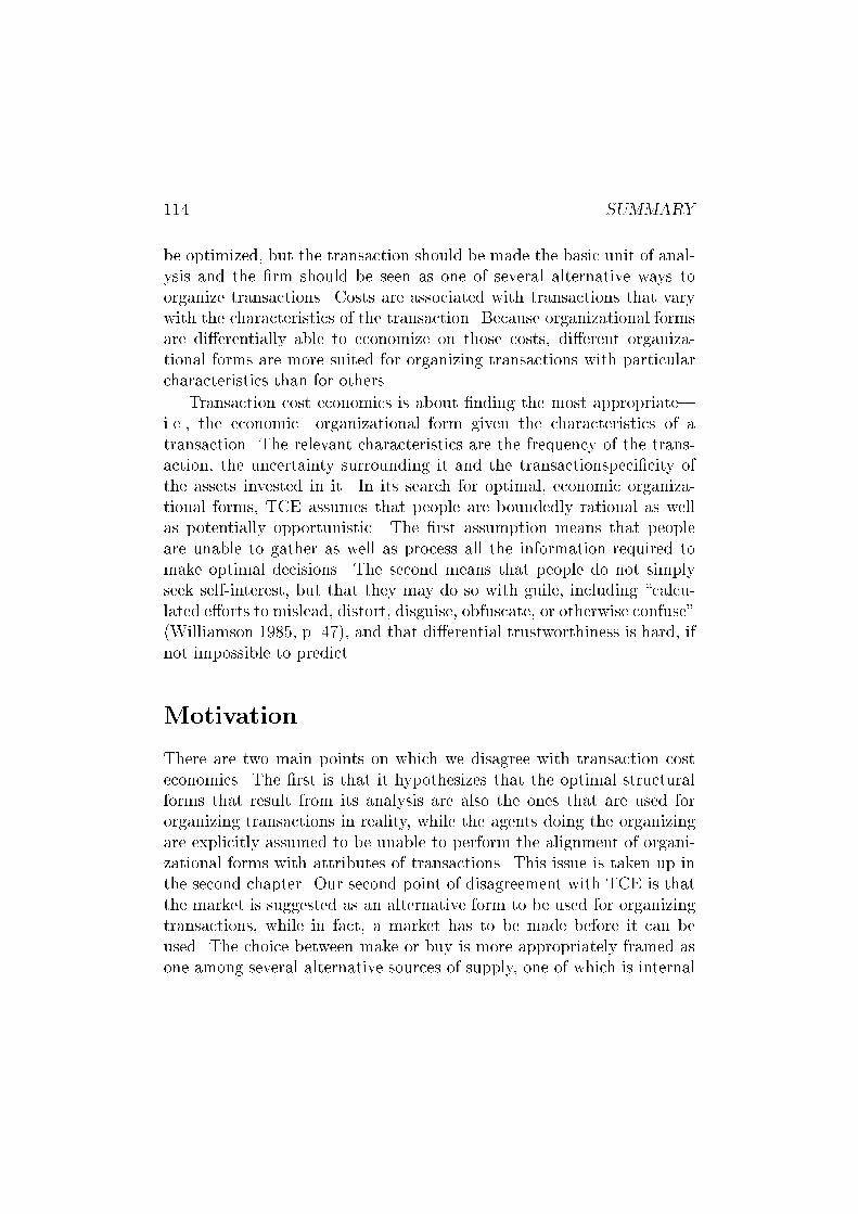
114 SUMMARY

be optimized, but the transaction should be made the basic unit of anal-

ysis and the �rm should be seen as one of several alternative ways to

organize transactions. Costs are associated with transactions that vary

with the characteristics of the transaction. Because organizational forms

are di�erentially able to economize on those costs, di�erent organiza-

tional forms are more suited for organizing transactions with particular

characteristics than for others.

Transaction cost economics is about �nding the most appropriate|

i.e., the economic|organizational form given the characteristics of a

transaction. The relevant characteristics are the frequency of the trans-

action, the uncertainty surrounding it and the transactionspeci�city of

the assets invested in it. In its search for optimal, economic organiza-

tional forms, TCE assumes that people are boundedly rational as well

as potentially opportunistic. The �rst assumption means that people

are unable to gather as well as process all the information required to

make optimal decisions. The second means that people do not simply

seek self-interest, but that they may do so with guile, including \calcu-

lated e�orts to mislead, distort, disguise, obfuscate, or otherwise confuse"

(Williamson 1985, p. 47), and that di�erential trustworthiness is hard, if

not impossible to predict.

Motivation

There are two main points on which we disagree with transaction cost

economics. The �rst is that it hypothesizes that the optimal structural

forms that result from its analysis are also the ones that are used for

organizing transactions in reality, while the agents doing the organizing

are explicitly assumed to be unable to perform the alignment of organi-

zational forms with attributes of transactions. This issue is taken up in

the second chapter. Our second point of disagreement with TCE is that

the market is suggested as an alternative form to be used for organizing

transactions, while in fact, a market has to be made before it can be

used. The choice between make or buy is more appropriately framed as

one among several alternative sources of supply, one of which is internal

MOTIVATION 115

to the �rm and some of which are external. There will be more informa-

tion available about some alternatives than about others. This connects

to TCE's view on opportunism which is based on the assumption \that

some individuals are opportunistic some of the time and that di�erential

trustworthiness is rarely transparent ex ante" (Williamson 1985, p. 64).

In TCE, since it is hard to tell who will be opportunistic when, oppor-

tunism is always considered possible, and measures to counter its e�ects

are always considered necessary.

The picture can be made clearer by introducting the distinction be-

tween room for and inclination towards opportunism (Nooteboom 1999b)

and by considering that actual opportunism is a function of the two. TCE

does not consider inclination towards opportunism, because \[i]nasmuch

as a great deal of information about trustworthiness or its absence that

is generated during the course of bilateral trading is essentially private

information (. . . ) knowledge about behavioral uncertainties is very un-

even. The organization of economic activity is even more complicated as

a result" (Williamson 1985, p. 59). In this thesis, however, the suggested

increase in the complication of the organization of economic activity is

not admitted as a justi�cation for not addressing the relevant informa-

tion about trustworthiness or its absence. Instead, individual agents are

modeled, including their private information that they generate during

the course of their bilateral exchanges with other individual agents.

Chapter 2 takes up our other point of disagreement with transaction

cost economics, that it hypothesizes outcomes consistent with a rational

analysis that the agents involved are assumed to be unable to carry out.

This is not to say that those outcomes can not occur, because the agents

may stumble upon them by accident or luck, for example; objections are

raised against the argument underlying the hypothesis of e�cient out-

comes. This argument is one often used in economics more generally,

that behavior consistent with ine�cient outcomes will not occur because

it does not survive on markets. However, markets are not totally e�cient

in weeding out suboptimal behavior and in producing only optimal be-

havior. For optimal behavior to survive, it has to be present in the �rst

place, or be introduced during the selection process, which may not hap-

116 SUMMARY

pen because of barriers to entry. Even if the optimal behavior is present

in the population, it has to be transferred from one agent to the next,

which is not trivial and also not in the interest of the agent doing the

transfer who may therefore try to sabotage this transfer.

Furthermore, the evolutionary natural selection argument is argued to

be principally unsuited for described developments in economic systems.

Drawing a parallel with an earlier critique (Klos 1999) of an application of

a genetic algorithm, a computational model of an evolutionary processes,

to the study of economic systems (Miller 1996), the appropriateness of

the evolutionary metaphor is questioned. Agents typically only interact

with other agents somehow close to them rather than with all other

agents, and they are not given new behavior by an evolutionary process,

but decide on changing their strategy themselves, based on a comparison

with others close to them.

An Agent-based Approach

In order to cope with the two objections raised against (transaction cost)

economics, an alternative, agent-based approach is proposed. This allows

individual agents to trust and act upon their private knowledge and to

make their own decisions about adapting their behavior in their search for

better performance. The agents are allowed to adopt any possible form

of behavior if they expect to bene�t from it. They are also allowed to

experiment and innovate and to make mistakes. In such a setting, it can

be investigated whether|rather than assumed that|e�cient outcomes

arise. Because such systems of adaptive agents of any reasonable size are

intractable analytically, we resort to computer simulations.

Chapter 3 describes the simulation model used. In each one of a

sequence of timesteps, individual �rms are confronted with the prob-

lem of organizing a transaction. On a �nal-goods market, they sell a

product with a certain level of di�erentiation. They have to decide be-

tween making and buying a component required to produce their prod-

uct. They do so in each of a number of timesteps, and base decisions in

AN AGENT-BASED APPROACH 117

current timesteps on their experiences in previous timesteps, which are

co-determined by the other agents' decisions.

Assets that a supplier invests in to produce the component for a buyer

are speci�c to the transaction with the buyer to the extent that the buy-

er's product is di�erentiated. Suppliers may build up economies of scale

in their accumulation of non-speci�c assets across the production for mul-

tiple buyers, and economies of learning in their continued, uninterrupted

use of buyer-speci�c assets in their production for a particular buyer.

Buyers are assigned to a supplier (in which case they buy the compo-

nent) or to themselves (in which case they make the component) on the

basis of buyers' preferences for being matched to each one of a number of

possible suppliers and to themselves and on the basis of suppliers' pref-

erences for being matched to each one of the buyers. This is done by a

so-called matching algorithm, i.c. Tesfatsion's (1997) Deferred Choice and

Refusal (DCR) algorithm. Preferences are based on scores that agents

assign to each other and on their loyalty for their current partner, if they

have one. Loyalty means that the agents prefer their current partner

over alternatives as long as the scores they assign to alternatives do not

exceed the score they assign to their current partner by at least a certain

threshold, � .

Scores are a function of pro�tability and trust: in essence, scores ex-

press expected pro�t|potential pro�t multiplied with the agent's trust

in the other agent as an expression of the agent's subjective probability

that the other agent will not behave opportunistically, but let him realize

that potential pro�t. Because we want agents to be able to put di�eren-

tial weights on pro�tability versus trust, however, each agent raises other

agents' pro�tability to the power of the value it uses for � and their trust

to the power of (1 � �). Buyers contribute to pro�tability through the

positive e�ect that the di�erentiation of their products has on the re-

turns they generate, while suppliers contribute to pro�tability through

the negative e�ect that their economies of scale and learning have on

the costs of production. Buyers are not able to produce with e�ciency

higher than 0. Any pro�ts made in a relation are shared among the two

agents involved.

The agents' adaptation refers to the fact that they change their trust

118 SUMMARY

in other agents on the basis of their experiences in mutual interactions as

well as the values they use for � and � . There are di�erent values possible

for each and in each timestep, when they need them for establishing

preferences, the agents choose one value for each.

Chapter 4 presents and discusses the results from experiments with

the model. First of all, a parametersetting has been chosen that make

the results sensitive, but not too sensitive to changes in experimental

variables. Then, the plausibility of the model was tested. A result from

TCE that is not disputed here is the relation between increasing transac-

tionspeci�city of assets and an increasing proportion of economic activity

that is organized internally rather than on the market. This relation was

found in the results of a series of experiments in which the di�erentiation

of the buyers' products on the �nal market was increased.

With some con�dence in the model's sensitivity and plausibility, the

two points of criticism of transaction cost economics could be dealt with.

Concerning the investigation rather than assumption of e�cient out-

comes, it was established that the optimum is often not reached in a

complex system of boundedly rational, adaptive agents. Only rarely

does the system, by coincidence, develop a situation that is optimal for

all agents involved. As for the second point of criticism, a direct com-

parison between TCE and our model is much harder, because TCE does

not mention trust. It appears from the results that the agents learn to

put slightly stronger emphasis on pro�tability than on trust. A more

general conclusion that can be drawn from the results is that individual

agents need to be investigated in order to understand what happens in

the system.

Samenvatting

(Summary in Dutch)

Inleiding

Dit proefschrift gaat over het organiseren van transacties. Een transactie

betekent dat een goed of dienst een technologische grens overschrijdt, wat

het geval is als de ene activiteit ophoudt en de andere begint. Er zijn ver-

schillende structuren waarin activiteiten kunnen worden georganiseerd.

Beide activiteiten die door een transactie met elkaar worden verbonden

kunnen bijvoorbeeld binnen �e�en en hetzelfde bedrijf worden onderge-

bracht, in welk geval de hi�erarchie binnen het bedrijf wordt gebruikt

om de transactie te organiseren. De beide activiteiten zouden, aan de

andere kant, ook over verschillende gespecialiseerde bedrijven kunnen

worden verdeeld, in welk geval de markt wordt gebruikt om de trans-

actie te organiseren. In wat bekendere terminologie moet een bedrijf

besluiten activiteiten uit te besteden of zelf uit te voeren, dat wil zeggen

om componenten zelf te maken of te kopen.

Hoofdstuk 1 beschrijft de theoretische achtergrond van het onderzoek.

Transactiekostentheorie (TCE voor Transaction Cost Economics) wordt

vaak gebruikt om het make-or-buy probleem te analyseren, maar ook voor

vele andere organisatieproblemen. Deze theorie is ontstaan uit de pu-

blicatie The Nature of the Firm door Coase (1937) en verder ontwikkeld

door, onder andere, Williamson (1975, 1985). Coase (1937, p. 390) vroeg

zich af \why a �rm emerges at all in a specialised exchange economy",

119

120 SAMENVATTING (SUMMARY IN DUTCH)

en \why co-ordination is the work of the price mechanism in one case

and of the entrepreneur in another" (1937, p. 389). Volgens Coase en

de transactiekostentheorie in het algemeen, moet de onderneming niet in

isolement worden bestudeerd als een te optimaliseren productiefunctie,

maar moet de transactie eenheid van analyse worden gemaakt en moet

de onderneming worden beschouwd als �e�en van een aantal alternatieve

manieren om transacties te organiseren. Aan het organiseren van trans-

acties zijn kosten verbonden die vari�eren met de eigenschappen van trans-

acties. Aangezien verschillende organisatievormen in verschillende mate

in staat zijn op deze kosten te besparen, zijn sommige organisatievormen

voor het organiseren van transacties met bepaalde eigenschappen meer

geschikt dan (voor) andere.

Transactiekostentheorie gaat over het vinden van de meest geschikte|

dat wil zeggen de meest economische|organisatievorm, gegeven de eigen-

schappen van de transactie. Relevante eigenschappen zijn de frequen-

tie van de transactie, de mate waarin de transactie door onzekerheid is

omgeven en de transactiespeci�citeit van activa. In de analyse van op-

timale, economische organisatievormen, veronderstelt TCE dat mensen

beperkt rationeel zowel als mogelijk opportunistisch zijn. De eerste

veronderstelling houdt in dat mensen niet in staat zijn alle voor optimale

beslissingen benodigde informatie te verzamelen en te verwerken. De

tweede veronderstelling houdt in dat mensen niet slechts hun eigenbelang

nastreven, maar dat ze hierbij ook list en bedrog inschakelen, inclusief

\calculated e�orts to mislead, distort, disguise, obfuscate, or otherwise

confuse" (Williamson 1985, p. 47), en dat individuele betrouwbaarheid

moeilijk, zo niet onmogelijk vast te stellen is.

Motivatie

Op twee punten verschillen we met transactiekostentheorie van mening.

Het eerste is dat TCE stelt dat de optimale structuren die resulteren

uit haar rationele analyse ook de structuren zijn die in de werkelijkheid

voor het organiseren van transacties worden gebruikt, terwijl tegelijker-

tijd degenen die organiseren expliciet verondersteld worden niet in staat

MOTIVATIE 121

te zijn organisatievormen optimaal op de eigenschappen van transacties

af te stemmen. Op dit punt wordt in hoofdstuk 2 ingegaan. Ons tweede

punt van kritiek is dat de markt wordt gesuggereerd als een van de al-

ternatieve manieren die kunnen worden gebruikt om transacties mee te

organiseren, terwijl een markt moet worden gemaakt voordat hij kan

worden gebruikt. De keuze tussen kopen en zelf maken kan beter worden

gezien als de keuze tussen een aantal alternatieve toeleveringsbronnen,

waarvan er zich �e�en binnen de onderneming bevindt en een aantal buiten

de onderneming. Over sommige bronnen zal meer informatie beschik-

baar zijn dan over andere. Dit sluit aan bij het perspectief van TCE op

opportunisme, dat gebaseerd is op de assumptie \that some individuals

are opportunistic some of the time and that di�erential trustworthiness

is rarely transparent ex ante" (Williamson 1985, p. 64). Omdat het dus

moeilijk te voorspellen is wie zich wanneer opportunistisch zal gedragen,

wordt opportunisme altijd voor mogelijk gehouden en zijn maatregelen

om negatieve e�ecten ervan tegen te gaan altijd nodig.

Het beeld kan worden verhelderd door het onderscheid tussen ruimte

voor en neiging tot opportunisme te introduceren (Nooteboom 1999b) en

zich te realiseren dat feitelijk opportunisme een functie van beide is. TCE

beschouwt neiging tot opportunisme niet, omdat \[i]nasmuch as a great

deal of information about trustworthiness or its absence that is generated

during the course of bilateral trading is essentially private information

(. . . ) knowledge about behavioral uncertainties is very uneven. The or-

ganization of economic activity is even more complicated as a result"

(Williamson 1985, p. 59). In dit proefschrift echter, wordt de gesug-

gereerde toename in de complexiteit van de organisatie van economi-

sche activiteit niet toegelaten als verantwoording voor het niet gebruik

maken van relevante informatie over de aan- of afwezigheid van betrouw-

baarheid. In plaats daarvan worden individuele actoren beschouwd, in-

clusief hun priv�e informatie die ze verzamelen tijdens hun interacties met

andere actoren.

Hoofdstuk 2 gaat in op onze andere onenigheid met TCE, namelijk

dat de theorie uitkomsten veronderstelt die consistent zijn met een ra-

tionele analyse die de betrokken actoren volgens de assumptie van be-


perkte rationaliteit niet in staat zijn uit te voeren. Dit wil overigens

niet zeggen dat dergelijke uitkomsten niet voor kunnen komen, aangezien

de actoren er per ongeluk of toevallig voor zouden kunnen kiezen; ons

bezwaar is gericht tegen het argument voor de hypothese van optimale

uitkomsten. Dit argument wordt in de economische theorie vaak ge-

bruikt, namelijk dat gedrag consistent met niet-optimale uitkomsten niet

voor zal komen omdat het op markten niet overleeft. Markten zijn echter

niet volledig e�ectief in het verwijderen van suboptimaal gedrag en het

produceren van uitsluitend optimaal gedrag. Wil optimaal gedrag over-

leven, dan moet het aan het begin van dit evolutionaire proces al aan-

wezig zijn, of gedurende het proces tot stand kunnen komen, wat entree-

barri�eres kunnen tegenhouden. Zelfs al is het optimale gedrag op zeker

moment aanwezig, dan moet het van actor tot actor worden doorgegeven,

wat een niet triviaal proces is en bovendien niet in het belang van de

doorgevende actor, die het proces zal willen saboteren.

Afgezien van deze argumenten, wordt betoogd dat het evolutionaire

natuurlijke selectie argument in het algemeen ongeschikt is voor het mo-

delleren van ontwikkelingen in economische systemen. Aan de hand van

een eerdere kritiek (Klos 1999) van een toepassing van een genetisch

algoritme, een computationeel model van een evolutionair proces, voor

het bestuderen van economische systemen (Miller 1996), wordt tegen de

toepasselijkheid van de evolutionaire metafoor geargumenteerd. Actoren

interacteren normaal gesproken alleen met bepaalde andere actoren in de

`groep' waartoe ze behoren en niet met alle andere actoren. Ze worden

verder niet door een evolutionair proces nieuw gedrag gegeven, maar

beslissen zelf over het aanpassen van hun gedrag, op basis van een verge-

lijking met anderen in de groep waartoe ze behoren.

Een actorgebaseerde benadering

Om met de beide punten van kritiek tegen transactiekostentheorie in

het bijzonder en economische wetenschap in het algemeen om te kunnen

gaan, wordt een alternatieve, actorgebaseerde benadering voorgesteld.

Die benadering maakt het actoren mogelijk meer of minder vertrouwen

EEN ACTORGEBASEERDE BENADERING 123

in anderen te stellen, op basis van hun persoonlijke informatie over an-

deren te handelen en hun gedrag naar eigen goeddunken aan te passen in

hun zoektocht naar betere prestaties. De actoren wordt het in principe

toegestaan zich op elke mogelijke manier te gedragen, als ze menen daar

beter van te worden. Het wordt ze ook toegestaan te experimenteren en

te innoveren en fouten te maken. In een dergelijke omgeving kan wor-

den onderzocht of|in plaats van verondersteld dat|optimale uitkom-

sten optreden. Omdat dergelijke systemen van adaptieve actoren met

elke redelijke omvang niet analytisch te bestuderen zijn, is van computer

simulaties gebruik gemaakt.

Hoofdstuk 3 beschrijft het gebruikte computersimulatiemodel. In elk

van een reeks tijdsstappen, worden actoren geconfronteerd met het pro-

bleem een bepaalde transactie te organiseren. Ze verkopen een product

dat in een bepaalde mate gedi�erentieerd is. Ze moeten besluiten een

component dat voor de productie van hun product nodig is te kopen

of zelf te maken. Dit doen ze in elk van de tijdsstappen, waarbij ze

beslissingen in huidige tijdsstappen baseren op hun ervaringen in vorige

tijdsstappen, die deels worden be��nvloed door de beslissingen van andere

actoren.

Activa waarin door een leverancier wordt ge��nvesteerd ten behoeve

van de productie van het component voor een bepaalde afnemer zijn

speci�ek voor de transactie met die afnemer in dezelfde mate waarin

het product van de afnemer op de uiteindelijke markt gedi�erentieerd

is. Toeleveranciers kunnen schaalvoordelen opbouwen in niet-speci�eke

activa die ze gebruiken in hun productie voor meerdere afnemers en leer-

voordelen in hun continue, ononderbroken gebruik van afnemerspeci�eke

activa in hun productie voor die afnemer.

Afnemers worden aan een toeleverancier (in welk geval ze het com-

ponent kopen) of aan zichzelf (in welk geval ze het component maken)

toegewezen op basis van de preferenties van afnemers om aan elk van de

toeleveranciers danwel aan zichzelf te worden toegewezen en op basis van

de preferenties van de leveranciers om aan elk van de afnemers te wor-

den toegewezen. Deze toewijzing wordt uitgevoerd door een zogenaamd

toewijzingsalgoritme en meer bepaald door het Uitgestelde Keuze- en


Weigerings- (DCR voor Deferred Choice en Refusal) algoritme. De pre-

ferenties zijn gebaseerd op scores die actoren aan elkaar geven en op hun

loyaliteit voor hun huidige partner, als ze die hebben. Loyaliteit betekent

dat actoren hun huidige partner prefereren boven alternatieven zolang de

scores die ze aan alternatieven geven niet hoger zijn dan de score van hun

huidige partner plus een bepaalde drempel, � .

Scores zijn een functie van winstgevendheid en vertrouwen; in essen-

tie drukken scores verwachte winst uit|potenti�ele winst vermenigvuldigd

met het vertrouwen in de andere actor als een uitdrukking van de sub-

jectieve waarschijnlijkheid van de actor dat de andere actor zich niet

opportunistisch zal gedragen en hem in staat zal stellen dat winstpoten-

tieel ook daadwerkelijk te realiseren. Omdat we het de actoren echter

mogelijk willen maken verschillend belang aan winstgevendheid versus

vertrouwen te hechten, verheft elke actor de winstgevendheid van andere

actoren tot de macht � en zijn vertrouwen in andere actoren tot de macht

(1 � �). Afnemers dragen aan winstgevendheid bij via het positieve ef-

fect dat de di�erentiatie van hun product heeft op de opbrengsten die

ze genereren, terwijl leveranciers aan winstgevendheid bijdragen via het

negatieve e�ect dat hun schaal- en leervoordelen hebben op de kosten van

productie. Afnemers zelf kunnen geen schaal- of leervoordelen behalen.

Alle winst die in een relatie tussen twee actoren wordt behaald wordt

gedeeld.

Het adaptieve aspect van de actoren betreft het feit dat ze hun ver-

trouwen in andere actoren aanpassen op basis van hun ervaringen met

die anderen en dat ze de waarden aanpassen die ze gebruiken voor � en

� . Er zijn verschillende mogelijke waarden voor elk van beide parameters

en in elke tijdsstap, als ze een waarde nodig hebben, trekken ze er een op

basis van het succes dat ze in het verleden met de verschillende waarden

hebben behaald.

Hoofdstuk 4 presenteert en bespreekt de resultaten van experimenten

met het model. Ten eerste zijn parameterinstellingen gekozen die de re-

sultaten van het model wel gevoelig, maar niet te gevoelig voor veran-

deringen in de variabelen maken. Vervolgens is een test van de plausi-

biliteit van de resultaten van het model gedaan. Een hier niet betwist

EEN ACTORGEBASEERDE BENADERING 125

resultaat van TCE is de relatie tussen stijging van de transactiespeci-

�citeit van investeringen en stijging van het percentage activiteit dat in-

tern wordt georganiseerd in plaats van uitbesteed. Deze relatie is gevon-

den in een serie experimenten waarin de di�erentiatie van de producten

die afnemers op de uiteindelijke markt verkopen is opgevoerd.

Met enig vertrouwen in de gevoeligheid en de plausibiliteit van de

resultaten van het model, zijn vervolgens de beide punten van kritiek op

TCE behandeld. Wat de assumptie van optimale uitkomsten betreft, is

vastgesteld dat het optimum in veel gevallen niet wordt bereikt, wan-

neer een systeem van adaptieve actoren allemaal hun eigen prestaties

proberen te verhogen. Slechts in een enkel geval komt het systeem per

toeval terecht in een situatie die voor ieder optimaal is. Wat het tweede

kritiekpunt betreft valt een directe vergelijking veel moeilijker te maken

tussen wat TCE stelt en wat er daadwerkelijk uit het model komt, om-

dat TCE over vertrouwen en loyaliteit helemaal niets zegt. Het blijkt

uit de resultaten dat de actoren een licht sterkere nadruk leren te leggen

op winstgevendheid dan op vertrouwen. Een algemene conclusie is dat,

teneinde te begrijpen wat er in het systeem gebeurt, de analyse op het

niveau van individuele actoren plaats dient te vinden.

Stellingen

Behorende bij het proefschrift

AGENT-BASED COMPUTATIONAL

TRANSACTION COST ECONOMICS

Tomas Benjamin Klos

1. Loyaliteit staat efficiënt organiseren in de weg (ditproefschrift, hoofdstuk 4).

2. Het evolutionaire argument kan niet gebruikt worden omrationele analyses van optimale uitkomsten terechtvaardigen (dit proefschrift, hoofdstuk 2).

3. Uitkomsten van simulatie-experimenten worden te vaak tenonrechte als verrassende resultaten (‘emergent phenomena’)bestempeld. Dit kan voorkomen worden door van te vorenhet model goed te analyseren en na te denken over watverwacht mag worden.

4. Het feit dat aan een promotie-traject alleen al wordtbegonnen duidt op noodzakelijke, maar niet noodzakelijk opvoldoende bekwaamheid.

5. Elk promotie-traject voert over zijn eigen, specifiekefitness-landschap. De—tijdens het onderzoek zeerbruikbare—kaart van dit landschap kan pas aan het eind vanhet traject worden opgemaakt.

6. In de organisatie van aio-projecten wordt te weinig rekeninggehouden met het spanningsveld dat ontstaat door descheiding van het eigendom van en de controle opdergelijke projecten.

7. Teneinde het gevoel van eigendom over een project bij eenaio te vergroten, verdient het aanbeveling aio’s hun eigenonderzoeksvoorstel te laten schrijven.

8. Het feit dat de verlaging van transactiekosten door hettoepassen van moderne informatie- encommunicatietechnologie minder groot is dan hij zoukunnen zijn, heeft een psychologische en geen technischeoorzaak.

9. In de discussie over het al dan niet op geautomatiseerdewijze verzamelen van gegevens over het gedrag vaninternetgebruikers wordt te weinig rekening gehouden metde voordelen in termen van het afstemmen vandienstverlening op de (latente) behoeften van gebruikers ente veel gewezen op het vermeende big-brother karakterhiervan.

10. De stelling dat volgens randstedelingen de afstand vanGroningen naar de Randstad kleiner is dan de afstand van deRandstad naar Groningen, is alleen in de Randstad alsstelling de moeite waard.

11. De enige goede aio is geen aio.

Agent-based Computational Transaction Cost Economics

Documents

Transcript of Agent-based Computational Transaction Cost Economics