
Physics-based Modelling, Simulation, Placement and ...
222
Physics-based Modelling, Simulation, Placement and Learning for Musculo-Skeletal Animations Fabio Turchet A thesis submitted in partial fulfillment of the requirements of Bournemouth University for the degree of Doctor of Engineering Supervisors: Dr Oleg Fryazinov, Dr Sara Schvartzman January, 2018
-
Upload
khangminh22 -
Category
Documents
-
view
0 -
download
0
Transcript of Physics-based Modelling, Simulation, Placement and ...
Physics-based Modelling,
Simulation, Placement and
Learning for Musculo-Skeletal
Animations
Fabio Turchet
A thesis submitted in partial fulfillment of the requirements
of Bournemouth University for the degree of Doctor of
Engineering
Supervisors: Dr Oleg Fryazinov,
Dr Sara Schvartzman
January, 2018

Copyright statement
This copy of the thesis has been supplied on condition that anyone who
consults it is understood to recognise that its copyright rests with its
author and due acknowledgement must always be made of the use of any
material contained in, or derived from, this thesis.
i

Contents
Table of contents . . . . . . . . . . . . . . . . . . . . . . . . . vi
List of figures . . . . . . . . . . . . . . . . . . . . . . . . . . . xii
List of tables . . . . . . . . . . . . . . . . . . . . . . . . . . . xiii
Abstract . . . . . . . . . . . . . . . . . . . . . . . . . . . . . . xiv
Acknowledgements . . . . . . . . . . . . . . . . . . . . . . . . xv
Declaration . . . . . . . . . . . . . . . . . . . . . . . . . . . . xvi
I Introduction and Background 1
1 Introduction 2
1.1 Research Problems overview . . . . . . . . . . . . . . . . 2
1.2 Aims and Objectives . . . . . . . . . . . . . . . . . . . . 4
1.3 Character Effects Pipeline . . . . . . . . . . . . . . . . . 5
1.3.1 Musculo-skeletal Systems . . . . . . . . . . . . . . 7
1.4 The Companies . . . . . . . . . . . . . . . . . . . . . . . 8
1.4.1 Prime Focus World . . . . . . . . . . . . . . . . . 9
1.4.2 MPC . . . . . . . . . . . . . . . . . . . . . . . . . 9
1.4.3 Experience at Prime Focus in a nutshell . . . . . 10
1.4.4 Experience at MPC in a nutshell . . . . . . . . . 11
1.5 Contributions . . . . . . . . . . . . . . . . . . . . . . . . 13
1.6 Thesis Outline . . . . . . . . . . . . . . . . . . . . . . . . 14
2 Background 15
2.1 Anatomy Background . . . . . . . . . . . . . . . . . . . . 15
2.1.1 Bones . . . . . . . . . . . . . . . . . . . . . . . . 16
2.1.2 Muscles . . . . . . . . . . . . . . . . . . . . . . . 16
ii

2.1.3 Tendons . . . . . . . . . . . . . . . . . . . . . . . 18
2.1.4 Fascia . . . . . . . . . . . . . . . . . . . . . . . . 19
2.1.5 Fat . . . . . . . . . . . . . . . . . . . . . . . . . . 21
2.1.6 Skin . . . . . . . . . . . . . . . . . . . . . . . . . 21
2.1.7 Veins . . . . . . . . . . . . . . . . . . . . . . . . . 21
2.2 Muscle systems background . . . . . . . . . . . . . . . . 22
2.3 Solvers and Methods for Deformable Objects . . . . . . . 23
2.3.1 Offline Physics-Based Methods . . . . . . . . . . 26
2.3.2 Interactive and Real-Time Methods . . . . . . . . 29
2.3.3 Procedural Methods . . . . . . . . . . . . . . . . 30
2.3.4 Methods based on acquisition and machine learning 31
II Projects 38
3 Muscle Modelling 39
3.1 Introduction . . . . . . . . . . . . . . . . . . . . . . . . . 39
3.1.1 Muscle Primitives fixing . . . . . . . . . . . . . . 41
3.2 Related Work . . . . . . . . . . . . . . . . . . . . . . . . 43
3.3 Method . . . . . . . . . . . . . . . . . . . . . . . . . . . 44
3.3.1 Fibre Curves . . . . . . . . . . . . . . . . . . . . 45
3.3.2 Tendon Reconstruction . . . . . . . . . . . . . . . 46
3.3.3 Generation of muscles geometry . . . . . . . . . . 48
3.3.3.1 Elastic Model and Forces . . . . . . . . 49
3.3.4 Fibre Field . . . . . . . . . . . . . . . . . . . . . 52
3.4 Implementation and Results . . . . . . . . . . . . . . . . 53
4 Musculo-skeletal Simulation 56
4.1 Introduction . . . . . . . . . . . . . . . . . . . . . . . . . 56
4.2 Background . . . . . . . . . . . . . . . . . . . . . . . . . 56
4.2.1 Test 1: current MPC’s muscle system . . . . . . . 59
4.2.2 Test 2: only fat layer . . . . . . . . . . . . . . . . 59
4.2.3 Test 3: simulated passive muscles . . . . . . . . . 60
4.2.4 Test 4: simulated “active” muscles . . . . . . . . 61
4.2.5 Test 5: fascia driven by ”active” muscles and fat
layer driven by fascia . . . . . . . . . . . . . . . . 61
iii

4.2.6 Analysis of the tests . . . . . . . . . . . . . . . . 62
4.3 Solver and Material Models . . . . . . . . . . . . . . . . 63
4.3.1 Simulation Model Construction . . . . . . . . . . 63
4.3.2 Solver . . . . . . . . . . . . . . . . . . . . . . . . 64
4.3.3 Constitutive Material Model . . . . . . . . . . . . 70
4.3.4 Boundary Conditions (Constraints) . . . . . . . . 75
4.3.4.1 Springs view . . . . . . . . . . . . . . . 76
4.3.4.2 Constrained Dynamics view . . . . . . . 77
4.4 Implementation and Results . . . . . . . . . . . . . . . . 78
4.4.1 Bones . . . . . . . . . . . . . . . . . . . . . . . . 79
4.4.2 Muscles and Tendons . . . . . . . . . . . . . . . . 79
4.4.3 Fascia, Fat and Skin . . . . . . . . . . . . . . . . 85
5 Muscle Placement 97
5.1 Introduction . . . . . . . . . . . . . . . . . . . . . . . . . 97
5.2 Related Work . . . . . . . . . . . . . . . . . . . . . . . . 98
5.3 Method . . . . . . . . . . . . . . . . . . . . . . . . . . . 99
5.3.1 Initial muscle data preparation . . . . . . . . . . 100
5.3.2 Muscle placement . . . . . . . . . . . . . . . . . . 101
5.3.3 Sculpting . . . . . . . . . . . . . . . . . . . . . . 103
5.3.4 Simulation . . . . . . . . . . . . . . . . . . . . . . 105
5.4 Implementation and Results . . . . . . . . . . . . . . . . 105
6 Implicit Skinning Extension 108
6.1 Introduction . . . . . . . . . . . . . . . . . . . . . . . . . 108
6.2 Related work . . . . . . . . . . . . . . . . . . . . . . . . 109
6.3 Method . . . . . . . . . . . . . . . . . . . . . . . . . . . 111
6.3.1 Angle Fields Preparation . . . . . . . . . . . . . . 112
6.3.2 Curve Creation . . . . . . . . . . . . . . . . . . . 113
6.3.3 Wrinkle Field . . . . . . . . . . . . . . . . . . . . 115
6.3.4 Projection . . . . . . . . . . . . . . . . . . . . . . 116
6.3.5 Parameters . . . . . . . . . . . . . . . . . . . . . 117
6.4 Implementation and Results . . . . . . . . . . . . . . . . 118
7 Pilot Study on Deep Learning for Deformable Objects 126
iv

7.1 Introduction . . . . . . . . . . . . . . . . . . . . . . . . . 126
7.1.1 Background . . . . . . . . . . . . . . . . . . . . . 127
7.2 Related Work . . . . . . . . . . . . . . . . . . . . . . . . 130
7.3 Dataset . . . . . . . . . . . . . . . . . . . . . . . . . . . 131
7.4 Architecture . . . . . . . . . . . . . . . . . . . . . . . . . 133
7.4.1 Method based on images / UV . . . . . . . . . . 134
7.4.2 Geodesic Convolution . . . . . . . . . . . . . . . . 136
7.5 Cost Functions . . . . . . . . . . . . . . . . . . . . . . . 137
7.5.1 Constraints . . . . . . . . . . . . . . . . . . . . . 138
7.5.2 Future frames data augmentation . . . . . . . . . 139
7.5.3 Future frames partial derivatives accumulation . . 139
7.5.4 RNN . . . . . . . . . . . . . . . . . . . . . . . . . 140
7.5.5 Unsupervised Loss Function . . . . . . . . . . . . 141
7.5.6 SpatioTemporal Convolution . . . . . . . . . . . . 141
7.6 Training and Testing Process . . . . . . . . . . . . . . . 142
7.7 Implementation and Results . . . . . . . . . . . . . . . . 146
III Conclusions and Future Work 168
8 Conclusions and Future Work 169
8.1 Conclusions . . . . . . . . . . . . . . . . . . . . . . . . . 169
8.1.1 Muscle primitives modelling . . . . . . . . . . . . 171
8.1.2 Muscle simulation framework . . . . . . . . . . . 172
8.1.3 Placement of simulation-ready muscles . . . . . . 172
8.1.4 Procedural wrinkles . . . . . . . . . . . . . . . . . 173
8.1.5 Deep learning for deformable objects . . . . . . . 174
8.2 Future Work . . . . . . . . . . . . . . . . . . . . . . . . . 174
References 178
A List of publications 192
B Material Derivation 193
B.1 Muscle material. Energy formula . . . . . . . . . . . . . 193
C Material Derivation (cont.) 200
v

C.1 Derivation of dPdF for StVk material . . . . . . . . . . . 200
D EngD Experience Conclusions 204
vi
List of Figures
1.1 Simplified 3D movie production pipeline. . . . . . . . . . 5
2.1 Skin anatomy. From top to bottom: epidermis (skin),
dermis, fat tissue, muscle c© (Massage Research 2013). . 16
2.2 Hierarchical structure of a striated muscle (Lee et al. 2012).
. . . . . . . . . . . . . . . . . . . . . . . . . . . . . . . . 17
2.3 Types of muscles based on their shape and internal fibres
architecture (Lee et al. 2012). . . . . . . . . . . . . . . . 18
2.4 Fascia at work c© (Fortier 2013). . . . . . . . . . . . . . 19
2.5 c© Fascia fibres (Myotherapies 2013). . . . . . . . . . . 20
2.6 Front, back and side muscles of arm and torso (MPC mus-
cles generated from anatomical sheets). . . . . . . . . . . 24
3.1 A slice of the arm muscle primitives showing intricate in-
tersections. . . . . . . . . . . . . . . . . . . . . . . . . . 41
3.2 (a) intersecting geometries of the forearm; (b) solved in-
tersections, (c) highlighted fixed areas. . . . . . . . . . . 42
3.3 Overview of the pipeline. (a) Input skin mesh and skele-
ton; (b) sketched patches of superficial muscles; (c) in-
flated output muscles (opacity used to show underlying
structures) ; (d) associated fibres . . . . . . . . . . . . . . 44
3.4 Frames at progressive times of the extension of fibre curves
for tendon reconstruction via the use of a flocking system. 46
vii

3.5 Top: initial bicep patch segmented from the character’s
skin; initial fibre curves in green; point sets SP and EP
in magenta and cyan; target point sets ASP and AEP in
red and blue, respectively; bottom: tendon reconstruction
via flock simulation. . . . . . . . . . . . . . . . . . . . . . 47
3.6 (a) Deltoid extruded patch; (b) inflated muscle; (c) new
rest shape after smoothing and relaxation. . . . . . . . . 48
3.7 (a) Deltoid extruded patch with collision objects; (b) par-
tial inflation; (c) full inflation. . . . . . . . . . . . . . . . 50
3.8 Slices at different depth of the inflated muscles of the arm.
Depth of the slicing plane increasing progressively from (a)
to (f). . . . . . . . . . . . . . . . . . . . . . . . . . . . . 53
3.9 (a) Generated bicep muscle; (b) Fibre curves and interpo-
lated internal fibres; (c) Rest pose mesh; (d) Embedded
mesh of deformed pose obtained using a tetrahedral FEM
simulation with anisotropic material (isometric contrac-
tion). . . . . . . . . . . . . . . . . . . . . . . . . . . . . 55
4.1 (a) Slice of the full volumetric model; (b) Renderable skin 58
4.2 (a) Shrunk fascia; (b) fat volumetric layer . . . . . . . . 59
4.3 (a) Skeleton ; (b) Attached muscles; (c) Muscle deformation 60
4.4 (a) Line muscles with driving sphere volumes for attach-
ment (in yellow) . . . . . . . . . . . . . . . . . . . . . . 61
4.5 Deformation of (a) Muscles; (b) Fascia; (c) Fat; (d) Ren-
derable skin . . . . . . . . . . . . . . . . . . . . . . . . . 62
4.6 Anatomical geometry for prototype testing. On the left
the renderable/embedded mesh from which its conforming
volumetric counterpart is generated (right). . . . . . . . . 65
4.7 Transverse isotropy . . . . . . . . . . . . . . . . . . . . 70
4.8 Material response of muscle fibre (active), tendons (pas-
sive) and their combination. (Teran et al. 2003) . . . . . 72
4.9 Temporal frames extracted from an animation of the humerus
rotating with biceps brachii having non activated fibres. . 81
4.10 Temporal frames extracted from an animation of the humerus
rotating with biceps brachii having activated fibres. . . . 82
viii
4.11 Full arm simulation. View 1. . . . . . . . . . . . . . . . . 88
4.12 Full arm simulation. View 1. (cont.) . . . . . . . . . . . 89
4.13 Full arm simulation. View 2. . . . . . . . . . . . . . . . . 90
4.14 Full arm simulation. View 2. (cont.) . . . . . . . . . . . 91
4.15 Full arm simulation. View 3. . . . . . . . . . . . . . . . . 92
4.16 Full arm simulation. View 3. (cont.) . . . . . . . . . . . 92
4.17 Full arm simulation layers. View 1. Muscles in red, fascia
in yellow and fat/skin in blue. . . . . . . . . . . . . . . . 93
4.18 Full arm simulation layers. View 1. Muscles in red, fascia
in yellow and fat/skin in blue. (cont.) . . . . . . . . . . . 94
4.19 Full arm simulation layers. View 2. Muscles in red, fascia
in yellow and fat/skin in blue. . . . . . . . . . . . . . . . 95
4.20 Full arm simulation layers. View 2. Muscles in red, fascia
in yellow and fat/skin in blue. (cont.) . . . . . . . . . . . 96
5.1 Main steps of the system for a scene with biceps brachii
and brachialis muscles. From left to right: (a) rest shape
of a muscle; (b) dynamic placement; (c) context-aware
sculpting of intersection-free geometry with tetrahedral
cage deformation; (d) simulation with contraction of the
newly created muscle. . . . . . . . . . . . . . . . . . . . . 100
5.2 Input tetrahedral and embedded meshes for the biceps
brachii. Highlighted in green and with a semi-transparent
shader is the low resolution tetrahedral cage. In dark gray
the underlying high resolution embedded mesh. . . . . . 100
5.3 Placement of the tendon handles in place over the humerus
bone. . . . . . . . . . . . . . . . . . . . . . . . . . . . . . 102
5.4 Sculpting tool interface in Maya. . . . . . . . . . . . . . 103
5.5 Some steps of the sculpting process in which the mesh is
pushed out but collides with an existing adjacent muscle
(in gray). The red circle represents the Maya brush gizmo.
The wrap deformer acts in real-time at each brush stroke,
in this figure from the embedded mesh in red onto the
cage in pink. . . . . . . . . . . . . . . . . . . . . . . . . . 104
ix

5.6 Some steps of the simulation process, in which the bending
of the elbow joint activates the contraction of the biceps
brachii. . . . . . . . . . . . . . . . . . . . . . . . . . . . . 105
6.1 Overview of the workflow of the system. (a) Angle field
gradients; (b) Seeds and curves; (c) Final result (meshes
are subdivided); (d) Real example of a left thumb. . . . . 108
6.2 In pink f1 and blue f2, two HRBF fields; angles between
their gradients are shown in yellow. . . . . . . . . . . . . 111
6.3 Angle field generation using one-ring neighbours (a) and
connected vertices (b). . . . . . . . . . . . . . . . . . . . 121
6.4 Wrinkles generated from the fields in Figure 6.3. . . . . . 122
6.5 Plugin Parameters. . . . . . . . . . . . . . . . . . . . . . 123
6.6 (a) Default Dual Quaternion skinning; (b) Implicit Skin-
ning; (c) Angle gradient field (non biased); (d) Seeds and
curves; (e) Wrinkles after projection; (f) Picture of a real
thumb. . . . . . . . . . . . . . . . . . . . . . . . . . . . 124
6.7 Comparison of the results obtained for an arm. (a)-(d)
front and back views using topology biased field; (e)-(h)
front and back views using normal, non biased field. . . 125
7.1 Lee et al. (2011) . . . . . . . . . . . . . . . . . . . . . . 128
7.2 Low and high resolution plane geometries used for the
dataset creation, with constraining objects on two of the
sides. . . . . . . . . . . . . . . . . . . . . . . . . . . . . . 131
7.3 One frame of the animations for the scenes of the dataset. 132
7.4 Architecture of the convolutional neural network. . . . . 134
7.5 Input velocity field in UV space . . . . . . . . . . . . . . 135
7.6 Input velocity field in UV space in Voronoi style . . . . . 135
7.7 Training (blue) and testing (red) curves for low res loss
with future samples. . . . . . . . . . . . . . . . . . . . . 143
7.8 Training (blue) and testing (red) curves for low res loss
with future partial derivatives. . . . . . . . . . . . . . . . 144
7.9 Training (blue) and testing (red) curves for low res loss
with RNN. . . . . . . . . . . . . . . . . . . . . . . . . . . 145
x

7.10 Training (blue) and testing (red) curves for high res loss
with future samples. . . . . . . . . . . . . . . . . . . . . 147
7.11 Training (blue) and testing (red) curves for high res loss
with future partial derivatives. . . . . . . . . . . . . . . . 148
7.12 Training (blue) and testing (red) curves for high res loss
with RNN. . . . . . . . . . . . . . . . . . . . . . . . . . . 149
7.13 Training (blue) and testing (red) curves for high res loss
with unsupervised loss function. . . . . . . . . . . . . . . 149
7.14 Training (blue) and testing (red) curves for high res loss
without future samples for images. . . . . . . . . . . . . 150
7.15 Training (blue) and testing (red) curves for high res loss
with future samples for images. . . . . . . . . . . . . . . 150
7.16 Training (blue) and testing (red) curves for high res loss
with future partial derivatives. . . . . . . . . . . . . . . . 151
7.17 Training (blue) and testing (red) curves for high res loss
with RNN for images. . . . . . . . . . . . . . . . . . . . . 151
7.18 Training (blue) and testing (red) curves for high res loss
with spatio-temporal convolution for images. . . . . . . . 152
7.19 Low res pairs of results (predicted, ground truth) for sam-
pled frames in range 100-160 of the testing scene for RNN. 153
7.20 Low res pairs of results (predicted, ground truth) for sam-
pled frames in range 100-160 of the testing scene for partial
derivatives. . . . . . . . . . . . . . . . . . . . . . . . . . 154
7.21 Low res pairs of results (predicted, ground truth) for sam-
pled frames in range 100-160 of the testing scene for future
samples. . . . . . . . . . . . . . . . . . . . . . . . . . . . 155
7.22 High res pairs of results (predicted, ground truth) for sam-
pled frames in range 100-160 of the testing scene for RNN. 157
7.23 High res pairs of results (predicted, ground truth) for sam-
pled frames in range 100-160 of the testing scene for partial
derivatives. . . . . . . . . . . . . . . . . . . . . . . . . . 158
7.24 High res pairs of results (predicted, ground truth) for sam-
pled frames in range 100-160 of the testing scene for future
samples. . . . . . . . . . . . . . . . . . . . . . . . . . . . 159
xi

7.25 High res pairs of results (predicted, ground truth) for sam-
pled frames in range 100-160 of the testing scene for un-
supervised loss. . . . . . . . . . . . . . . . . . . . . . . . 160
7.26 High res pairs of results (predicted, ground truth) for sam-
pled frames in range 100-160 of the testing scene without
future samples (images). . . . . . . . . . . . . . . . . . . 161
7.27 High res pairs of results (predicted, ground truth) for sam-
pled frames in range 100-160 of the testing scene for future
samples (images). . . . . . . . . . . . . . . . . . . . . . . 162
7.28 High res pairs of results (predicted, ground truth) for sam-
pled frames in range 100-160 of the testing scene for partial
derivatives (images). . . . . . . . . . . . . . . . . . . . . 163
7.29 High res pairs of results (predicted, ground truth) for sam-
pled frames in range 100-160 of the testing scene for RNN
(images). . . . . . . . . . . . . . . . . . . . . . . . . . . . 164
7.30 High res pairs of results (predicted, ground truth) for
sampled frames in range 100-160 of the testing scene for
spatio-temporal (images). . . . . . . . . . . . . . . . . . 165
7.31 UVs. Nodes corresponding to the rendered 2D mesh for
field values interpolation in green. . . . . . . . . . . . . . 166
B.1 Formulas reproduced from Blemker 2005 paper. . . . . . 197
xii

List of Tables
1.1 List of contributions . . . . . . . . . . . . . . . . . . . . 14
2.1 Comparison of deformable objects methods . . . . . . . . 32
xiii
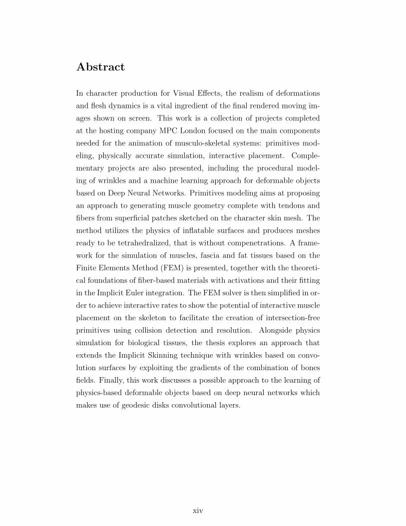
Abstract
In character production for Visual Effects, the realism of deformations
and flesh dynamics is a vital ingredient of the final rendered moving im-
ages shown on screen. This work is a collection of projects completed
at the hosting company MPC London focused on the main components
needed for the animation of musculo-skeletal systems: primitives mod-
eling, physically accurate simulation, interactive placement. Comple-
mentary projects are also presented, including the procedural model-
ing of wrinkles and a machine learning approach for deformable objects
based on Deep Neural Networks. Primitives modeling aims at proposing
an approach to generating muscle geometry complete with tendons and
fibers from superficial patches sketched on the character skin mesh. The
method utilizes the physics of inflatable surfaces and produces meshes
ready to be tetrahedralized, that is without compenetrations. A frame-
work for the simulation of muscles, fascia and fat tissues based on the
Finite Elements Method (FEM) is presented, together with the theoreti-
cal foundations of fiber-based materials with activations and their fitting
in the Implicit Euler integration. The FEM solver is then simplified in or-
der to achieve interactive rates to show the potential of interactive muscle
placement on the skeleton to facilitate the creation of intersection-free
primitives using collision detection and resolution. Alongside physics
simulation for biological tissues, the thesis explores an approach that
extends the Implicit Skinning technique with wrinkles based on convo-
lution surfaces by exploiting the gradients of the combination of bones
fields. Finally, this work discusses a possible approach to the learning of
physics-based deformable objects based on deep neural networks which
makes use of geodesic disks convolutional layers.
xiv

Acknowledgements
I would like to express my most sincere gratitude to the CDE and my
supervisors: Dr Oleg Fryazinov, Dr Sara Schvartzman and Dr Marco
Romeo. Without their encouragement, invaluable support and patience
none of this work would have been possible: I know there were moments
you wanted to kill me, but I’m glad I’m still alive.
Special thanks to the great people at MPC and Technicolor: the man-
agement team, in particular Georg, Rob and Hannes for believing in my
brain potential and in the benefits of long-term research; all the talented
colleagues in the Software and Rigging departments for the feedback and
the many joyful after-work drinking times: some of you are truly good
friends; Jamie Portsmouth for his great help with formulas derivations;
Vlad for the good laughs, discussions and for forcing me many times to
unglue myself from the chair and take some fresh air out.
Very special thanks to NVIDIA corporation for the donation of a Titan
Xp card as part of their GPU grant program.
I also wish to express my sincere appreciation to all the great teach-
ers and researchers I met in these four years at conferences around the
world: I am grateful for all the passion you put in your work, for being
visionaries, for demonstrating that often impossible is just a word and for
releasing extremely useful open source material for education purposes.
I would like to thank here my dearest friends who enriched so much
my life while staying in London: Pedro and Federico for being fantastic
humans and for always being there in the good and bad times; the Por-
tuguese crew for all the parties; Lucie, Ania and Nia for reminding me
to believe in my dreams and that Life is truly beautiful; my flatmates in
London for always giving me a smile when I came back home very late
and never made me feel I was just a crazy scientist.
Last but not least, I would like to address my biggest and warmest
acknowledgement to my family: my parents for constantly and uncondi-
tionally supporting me with their love in every possible way during these
roller-coaster years; my aunt Antonietta for the best inspirational quotes
and finally my brother Luca just for being the strongest person I know.
xv

Declaration
This report has been created by myself and has not been submitted in
any previous application for any degree. The work in this report has
been undertaken by myself except where otherwise stated.
xvi

Part I
Introduction and Background
1

Chapter 1
Introduction
Visual Effects (VFX) is a rather unique area of modern audio-visual pro-
ductions: in the same medium art and technology are blended together
to give the audience an emotional experience, ultimately supporting the
story that the director wants to tell. This thesis focuses on one of the
stages of the movie VFX production and in particular on the methods
and techniques used to make digital characters in motion look realistic.
In order to achieve this desired level of realism, physics-based animation
(PBA) is applied in such a way that the motion created by the animators
is enhanced by the physically plausible deformation of anatomical tissues
(muscles, fascia, fat and skin). This deformation makes the character
look alive through effects such as jiggling, wrinkles and bulging, which,
overall, contribute to bridge the gap towards crossing the so-called un-
canny valley. In this chapter, topics such as the VFX pipeline, physics
solvers and anatomy are introduced to provide the necessary background
to follow the work and frame it in the global setting of movie production.
1.1 Research Problems overview
There are many reasons why a visual effects company specializing in
digital creatures should invest in innovation towards a physically-based
character deformation pipeline. First of all, the level of realism that
2

can be achieved is much higher than standard methods: the world is
volumetric, objects including bodies and tissues are not hollow (as mod-
elled typically in VFX), but dense and respond to the laws of physics,
collisions and contacts. Movies nowadays contain massive amount of
computer generated characters and it is important to not disappoint the
main customers of this industry: the people and the fans going to the
cinemas or paying for streaming services to watch amazing, thrilling mov-
ing pictures. Therefore it is crucial to deliver visually stunning, plausible
and integrated computer generated content.
Because we are immersed in our 3D world and our brains are so special-
ized in detecting anomalies in dynamic behaviours that conflict with our
internal expectation of physics, producing unrealistic deformations for
the body and the face of a character in motion would ruin the sense of
immersion of the beholder and these anomalies would be quickly picked
up, consciously or unconsciously. Our perception is tuned to the laws
of physics since childhood: for instance, in real-time we make inferences
and predictions about the trajectory that an object is taking or the jig-
gling of a body in motion, based on visual clues, structure and prior
knowledge about the material properties. This leads us to make predic-
tions that put in words would be for instance: “This character looks fat
and with a lot of mass therefore will move slower than a muscular and
fit one” , or: “This ball shot by a cannon looks like metal so it will not
bounce much when impacting with the ground”. Therefore, even though
an excessive stress on the physical accuracy of the simulations is not the
real goal pursued by Visual Effects artists, a physics-based approach to
anatomical simulation provides many benefits. Visual plausibility and
being faithful to the director’s vision are priority instead and it would be
an overkill adopting blindly a medical level accuracy in VFX, considering
the computation times and artistic effort required.
In practice, the choice of which character pipeline to adopt boils down to
deciding where to put the complexity of the process. Procedural deform-
ers and standard skinning techniques allow achieving quickly visually
good results, but require a lot of artistic effort in sculpting blend shape
correctives (i.e. deformed shapes with the same topology but different
3

vertex positions that get interpolated); dynamics have to be achieved
with simulations on top of the cached geometry or with fast deformers
that “fake” secondary movements. Despite giving great level of control,
the problem of this approach is that it relies exclusively on the artist’s
ability to animate, with several constraints such as volume preservation.
On the other hand an approach purely physics-driven instead puts the
complexity at the beginning of the chain. Even though artists have to
spend significant effort setting up the inputs of the system such as skele-
ton, muscles, fascia, and fat layer geometries, they can benefit at a later
stage from the use of realistic materials and accurate, predictable results.
Nevertheless, in practice the problems of this approach are at least as
many as its benefits: being so dependent on the accuracy of the inputs,
when changes have to be made at the beginning of the chain, often the ex-
pensive simulations have to be recomputed. In addition, controlling the
behaviour of the solver (which has to solve for collisions, material model
forces, constraints) and the shape of the resulting anatomical model is
not a trivial task, especially in a production environment.
1.2 Aims and Objectives
This work aims to avoid the drawbacks of purely physics-based ap-
proaches and is not intended to achieve medical level results. Rather
than focusing only on improving the speed of the solver itself by switch-
ing from FEM to other alternatives (Projective Dynamics (Bouaziz et al.
2014), PBD (Muller et al. 2007) and more recently XPBD (Macklin et al.
2016)), this work shows how to cope with the problems of complexity
arising from the rest of the pipeline, in particular its inputs. We can
say, using a mathematics metaphor, that the optimal character pipeline
is a weighted average of the costs and benefits of all the aforementioned
methods that maximizes the visual realism of the output and minimizes
its production cost by considering parameters such as: computation time,
difficulty to setup, effort required to correct the output, artistic control,
stability.
4
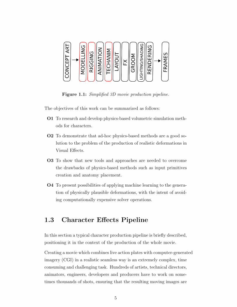
Figure 1.1: Simplified 3D movie production pipeline.
The objectives of this work can be summarized as follows:
O1 To research and develop physics-based volumetric simulation meth-
ods for characters.
O2 To demonstrate that ad-hoc physics-based methods are a good so-
lution to the problem of the production of realistic deformations in
Visual Effects.
O3 To show that new tools and approaches are needed to overcome
the drawbacks of physics-based methods such as input primitives
creation and anatomy placement.
O4 To present possibilities of applying machine learning to the genera-
tion of physically plausible deformations, with the intent of avoid-
ing computationally expensive solver operations.
1.3 Character Effects Pipeline
In this section a typical character production pipeline is briefly described,
positioning it in the context of the production of the whole movie.
Creating a movie which combines live action plates with computer-generated
imagery (CGI) in a realistic seamless way is an extremely complex, time
consuming and challenging task. Hundreds of artists, technical directors,
animators, engineers, developers and producers have to work on some-
times thousands of shots, ensuring that the resulting moving images are
5

consistent across the whole movie and that the story is conveyed at its
best. Figure 1.1 shows a simplified version of the pipeline of any 3D
moving picture production that uses computer generated assets. This is
briefly described in the following paragraphs.
Character production is just a part of the pipeline and like everything
else in the world of creative industries, it starts with an idea often in the
form of a description by words or rough sketches. Taking that initial idea,
the art department provides detailed concepts, proportions, exact mea-
surements, comparative scale sheets and scans (when available) in order
for the modellers to start creating initial versions of a mesh. The depart-
ments of interest for the scope of this work are Rigging and TechAnim.
Rigging is responsible for the creation of three kinds of setups: a low res-
olution puppet rig usable in real time by the animators; a facial setup;
a high resolution final quality rig comprising anatomy (skeletal bones,
dynamic muscles, fat, dynamic skin effects such as wrinkles). A variety
of solvers, deformers and techniques allow the completion of this task
for which the goal is to deliver to the next stages of the VFX pipeline
a high resolution mesh cache which deforms in a realistic way (a cache
is a file containing the encoding of the vertex positions per frame). The
rigging department collaborates closely with TechAnim who take care
of solving character effects problems that need ad-hoc solutions such as
contacts with other characters and objects and extra dynamics on the
tissues. This is often done on a shot by shot basis. After TechAnim, the
pipeline continues to lighting, shading and rendering. The sets produced
by layout, the digital matte paintings by the art department, the digital
effects (particles, fluids, destructions,explosions etc) and the curves by
the groom department and the animations are combined to produce the
final pixels of the images we admire on the screen.
The creation of a 3D character setup is often a long and iterative process.
In the case of digital doubles (perfect 3D digital versions of a real actor)
the anatomy is known a priori and the rigging process can start from a
human-like template. For a fantastic creature the process is similar, but
a greater amount of conceptualization work is needed to come up with
a plausible inner anatomy for it, often creating a unique set of bones
6

and muscles that never existed before. This task is informed by existing
anatomies of natural world species, often combining different parts of
them (for example in the case of a dragon-like creature the references
could be snakes, lizards, dinosaurs).
1.3.1 Musculo-skeletal Systems
There are areas of the Visual Effects pipeline that have received a lot
of attention since the early years of computer graphics research. In par-
ticular the simulation of natural phenomena such as water, gase and
fracturing of materials. Deformable objects have also been researched
for at least thirty years, but their application to anatomical simulation
and character effects is relatively recent, pushed and pioneered in par-
ticular by companies such as Weta Digital (Clutterbuck & Jacobs 2010),
MPC, ILM (Comer et al. 2015) and Framestore, who have to produce
photo-realistic CGI. “Muscle systems” as a broad term refers to a set
of techniques and workflows intended to reproduce in 3D the internal
anatomy shape and physical behaviour of human-like or fictional charac-
ters, with the goal of obtaining dynamic deformation of skin, flesh and
other biological tissues which is indistinguishable from reality. For a dis-
cussion of these tissues from an anatomical point of view, please refer to
Chapter 2.
A physics-based system for flesh simulation comprises various iterative
stages to be completed. First, based on anatomy atlases and previous
knowledge or scan data, modelling artists create the geometry of:
• Skeletal bones
• Muscles and tendons (mainly the superficial ones)
• Internal organs (optional)
• Fat tissue
• Skin (renderable geometry)
• Veins (optional)
7

• Facial blend shapes
This geometry should be ideally intersection-free, one of the reasons be-
ing that intersections would generate unwanted initial spurious contact
forces during simulation. For this purpose asset checking tools can be
used before sending the meshes down the pipeline. This problem is dis-
cussed in more detail along with potential solutions in Chapter 3 in
which a workflow for muscle placement that prepares simulation-ready
anatomical geometry is presented. Once the geometry is approved, rig-
gers place skeletal joints where articulation is needed, take care of the
skinning of the mesh to these transformation points, add deformers to
achieve procedural effects for sliding, contact and jiggling and custom
setups for props. Riggers also create the set of control gizmos for body
and face that animators will keyframe and from which animation curves
will be later exported.
One additional advantage of using an anatomy-based approach is con-
nected to the fact that rigging and character effects are just a part of
the larger movie VFX pipeline. In fact having the geometry and the
deformation of internal organs, veins, muscles, tendons, bones and fat
allows the rendering stage to achieve extremely visually realistic results,
by assigning different shaders (procedural programs that describe how
the light should interact with the geometry to render a desired mate-
rial look) to each layer and using complex subsurface scattering diffusion
algorithms for the outer skin. This, when paired with physically-based
rendering of materials, conveys a level of realism that requires less effort
than using geometry without internal anatomy. Research on anatomy-
based approaches constitutes the core of this work which was carried out
in two London based companies.
1.4 The Companies
My Engineering PhD (EngD) experience with the Centre of Digital En-
tertainment began with the first of two companies in which I completed
the 4 years programme. Prime Focus World gave the opportunity to
8

work on a variety of Research and Development (RnD) projects at their
London studio. A bit after the end of the first year though, the company
underwent a series of structural and business changes which led to lose
the researcher job position and forced to search for a new hosting com-
pany. After some interviews, I got offered a position at MPC London
to continue the EngD. Even though the topics of the research changed
after the transition, the main area stayed the same and MPC provided a
better research environment. Below is a summary of the two companies
and a brief description of the experience in terms of completed projects.
1.4.1 Prime Focus World
Prime Focus World (PFW) is a film-making partner to international stu-
dios and film production companies, providing world-class creative ser-
vices, pioneering technology services and intelligent financial solutions
on a global scale. From script to screen, PFW partners with produc-
tion companies and brands to develop and deliver animated CG content,
offering the scale and experience to deal with projects of any size. An-
imation credits include a number of full-length feature films and over
forty episodes of a fully CG animated TV show for a major global toy
brand. In 2014, PFW merged its VFX business with Double Negative
(Dneg), an Academy Award winning VFX industry leader with facilities
in London, Vancouver and Mumbai. PFW was the first company in the
world to convert a full Hollywood film from 2D to 3D, and its patented,
award-winning stereo conversion process has been used on more block-
buster Hollywood films than any other.
1.4.2 MPC
The Moving Picture Company (MPC) is a London based VFX house. It
has been one of the global leaders in VFX for over 25 years and count-
ing, with industry-leading facilities in London, Vancouver, Montreal, Los
Angeles, New York, Amsterdam, Bangalore and Mexico City. Some of
their most famous projects include blockbuster movies such as Godzilla,
9

the Harry Potter franchise, X-Men, Prometheus, Life of Pi, Guardians of
the Galaxy and The Jungle Book. The services they provide include con-
cept design, pre-viz, shoot supervision, 2D compositing, 3D/CG effects,
animation, motion design, software development, digital & experiential
production, colour grading for advertising and any combination of these
services.
1.4.3 Experience at Prime Focus in a nutshell
From October 2013 to early January 2013 I worked at Prime Focus on the
development of Nuke plugins for the View-D department. This depart-
ment is the one that focuses on the technology for the stereo conversion
of movies to stereoscopic 3D through proprietary software, in particu-
lar custom nodes for Eyeon Fusion. Therefore my initial tasks were to
convert some of these nodes to The Foundry’s Nuke compositing pack-
age. I developed various nodes (plugins) that were tools to analyze single
frames and sequences of images in order to visually and numerically de-
tect spurious pixels. These nodes were used for disparity maps and were
aimed to help the artist to find anomalies in sequences generated by
Ocula. One of these nodes made use of QT drawing tools to integrate
a dynamic histogram to facilitate the artist setting thresholds on a UI
rather than via float inputs. In that period I had the opportunity to learn
Nuke C++ NDK (API) and deepen my knowledge of QT. Starting from
mid January 2014, I could concentrate more on actual research and ex-
ploration of relevant topics. Therefore I started studying literature about
the techniques used in computer graphics for soft body deformation and
fracturing. The idea was to find ways to express materials in terms of
their microstructures to solve the problem of the lack of detail in the
internal parts of fractured objects. From there the interest shifted to the
modelling and simulation of heterogeneous materials because of the need
to approximate real world materials with more accuracy. Anisotropy is
a characteristic of many interesting real world materials and its appli-
cation to computer graphics is still somewhat limited, therefore worth
exploring. Towards the third quarter of the year, so around June 2014
10
the company proposed 2 topics:
• creation of huge vegetation landscapes and scenarios with opti-
mization both for modelling and rendering in mind. The system
had to be extremely efficient and user friendly and support effects
like wind and contact from characters, ideally crowds;
• large scale cloud simulation with fluids and control.
Therefore I started researching the simulation of clouds as a fluid and
other atmospheric effects. Unfortunately a few months later I lost the po-
sition because of the restructuring of the company and the clouds project
remained at the level of literature review and very early implementation.
1.4.4 Experience at MPC in a nutshell
At MPC there was the need to prototype a system to prove the potential
of the physics-based techniques developed in engineering and academic
settings. The first months at the company were spent implementing in
Maya and extending the Implicit Skinning framework (Vaillant et al.
2013), a procedural method that makes use of distance fields. This
proved to be a really good way to get used to the company tools and
practices. Also, it introduced me to the positive collaboration with my
Industrial Supervisor and the rest of the RnD team. Procedural meth-
ods are in general fast and work well for secondary characters, but hero
characters with detailed anatomy require more advanced techniques, es-
pecially to achieve good dynamics effects such as skin sliding and fat
jiggling. Therefore, the research proceeded towards the extension of an
open source Finite Elements library (Sin et al. 2013a) to create a system
for tissue simulation, equipped with constraints and fibre activation. It
gave the foundations and showed the path to use physics for other parts
of the character pipeline which constituted problems in a practical pro-
duction environment. In particular, even if the system showed good
potential, it became clear that the inputs of the systems and the way to
create rigs in this new anatomical manner were problematic and needed
to be addressed. In fact, in a real production, the solver itself constitutes
11

a necessary but not sufficient condition to achieve the results that rig-
gers and Effects Technical Directors (FX TDs) envision for the human or
creature under consideration. What makes the difference is not only the
presence of tools and methods to prepare the setup needed by the solver,
but also to control the behaviour of the solver (artistic control). This
constituted the motivation to carry on research for the primitive mod-
elling tool based on inflation and the interactive placement tool which, as
a by-product, led to publication. Another motivation for the shift from
the central importance of the solver and simulation method towards side
tools and techniques to help artists in the anatomical inputs work was
the fact that, concurrently to my experience at MPC, an external player
came to the market with a plugin for tissue simulation (Jacobs et al.
2016). The plugin was not adopted by MPC, a fact that confirmed the
will of the company to push instead on the existing proprietary internal
technology (successfully used for the Oscar-winning movie ’The Jungle
Book’ ) and carrying on Research and Development (RnD) on the tools
needed to ensure a proper transition to physics-based character anima-
tion. In that period towards the end of the third year, my industrial
supervisor changed.
In the final period of the EngD, driven both by personal interest and
MPC’s awareness of its growing potential, I started to focus on ma-
chine learning. Encouraged by some very recent existing research on
data-driven fluid simulation and other researchers in the mother com-
pany Technicolor, I dedicated my time towards a project using the now
popular Deep Neural Networks running on powerful Graphics Processing
Units (GPUs) with the goal of learning the physics of deformable objects
simulation. The outcomes of the project are described in Chapter 7.
Even though the prototypes developed have not been used in production,
at the end of this experience some valuable lessons have been learned to
improve future systems as discussed in part III.
In addition to the publications listed in appendix A, three software de-
partment presentations were given at MPC and one at a conference of a
leading company in rendering technology held in Sofia, Bulgaria (Chaos
12
Group 2015).
1.5 Contributions
Table 1.1 summarizes some of the problems described above; it contains
also the outcomes of the work in terms of public engagement and publi-
cations. The contributions consist of:
1. The creation of a custom simulation framework using FEM built
on top of the VEGA library to help the company in testing a
new physically-based approach to character deformation. Formu-
las were derived to implement muscle activations for a constitutive
material enriched with fibres. Constraints and collisions were also
added to the framework, contributing to the creation of a usable
prototype.
2. The creation of a novel method consisting of an interactive physics-
based design of muscle anatomical geometries ready to be simu-
lated.
3. The development of tools and techniques to interactively place mus-
cle geometries on a skeletal bones rig taking into consideration col-
lisions.
4. A procedural method for skinning using implicitly-defined scalar
fields was extended to create wrinkle effects.
5. The investigation of the application of Deep Learning to the sim-
ulation of deformable objects with the aim of improving the speed
of a standard solver.
The list of publications is presented in appendix A.
The five projects listed above are united by the common denominator
of the research and development of techniques to improve the realism of
character deformations in a movie pipeline. In fact, the muscle primitives
obtained with the superficial patch system can provide the input for both
the physics engine and the placement tool. The procedural wrinkle effects
13

Problem Contribution Publication/Outcome
Transition to PBA Tissue framework FMX 2015 presentation
Input setup Superficial patches Eurographics 2017
Artistic Control Muscle placement Siggraph 2016
Procedural Deformers Wrinkles for Implicit SkinningCVMP 2015 andSiggraph Asia 2015
Speed of the solver Deep learning Internal Presentation
Table 1.1: List of contributions
could be added as a post process on a coarse simulated geometry and the
pilot machine learning approach could be used at the end of the pipeline
to speed up the whole deformation system.
Besides this input/output logical connection, exploring procedural ap-
proaches as first project (in a chronological sense), also gave the possi-
bility of qualitatively evaluating the results later against physics based
approaches obtained with the simulator.
1.6 Thesis Outline
This thesis is structured as follows. In part I this first chapter provides
an introduction to the hosting companies, the character effects pipeline
adopted in modern movie production and an overview of the projects
completed; chapter 2 gives the necessary background on anatomy and a
general literature review on physics solvers. Part II describes five projects
(chapters 3-7) in a portfolio style: each one contains its own related
work and conclusions, explaining the relation and connection with the
other projects in an organic way. Part III discusses the results from
a global perspective and draws conclusions on the work done, together
with all the future work to improve the presented methods. Finally, a
list of publications and detailed derivations of formulas are shown in the
appendices.
14
Chapter 2
Background
The problems that this work tackle lie at the intersection of multiple
disciplines: anatomy, biomechanics, computer science, art production.
Therefore in this chapter some foundational knowledge on these areas
and notions will be given. First, the foundations of muscle and tissue
anatomy are given. In fact, the observation and the study of how re-
ality looks and works at a micro and macro level, inform the choices
of computer graphics techniques and algorithms. After presenting the
main anatomical components which are the scope of this research, the
chapter gives a broad level overview of what a muscle system is and its
use in Visual Effects. The chapter then continues by giving mathemati-
cal foundations of the equations governing the dynamics of motion in a
physics solver, in particular its standard and variational forms. Finally,
an extensive literature review of the existing approaches and methods
to deformable objects is given, dividing them in four main categories:
offline, interactive, procedural and learned methods.
2.1 Anatomy Background
There are over 650 muscles and 206 bones in the human body, with
the addition of various kinds of soft tissues presenting various degrees of
elastic material properties. The interaction of all these components dur-
15
ing motion increases the complexity of the resulting dynamics because
connected tissues are coupled and forces propagate in this intricate bi-
ological structure. In this research deep muscles that have negligible
effect on the surface appearance are simplified and discarded, bringing
the number down to about 110 and 100 relevant muscles and bones, re-
spectively.
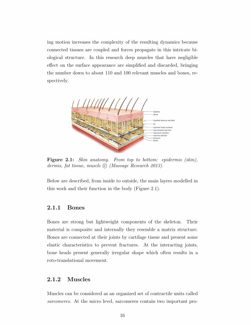
Figure 2.1: Skin anatomy. From top to bottom: epidermis (skin),dermis, fat tissue, muscle c© (Massage Research 2013).
Below are described, from inside to outside, the main layers modelled in
this work and their function in the body (Figure 2.1).
2.1.1 Bones
Bones are strong but lightweight components of the skeleton. Their
material is composite and internally they resemble a matrix structure.
Bones are connected at their joints by cartilage tissue and present some
elastic characteristics to prevent fractures. At the interacting joints,
bone heads present generally irregular shape which often results in a
roto-translational movement.
2.1.2 Muscles
Muscles can be considered as an organized set of contractile units called
sarcomeres. At the micro level, sarcomeres contain two important pro-
16

Figure 2.2: Hierarchical structure of a striated muscle (Lee et al. 2012).
teins called actin and myosin which chemically bind and overlap on
each other during contraction, thus being ultimately responsible for the
bulging look at a macro level, together with the conservation of volume
due to the contraction happening in a closed area made of incompressible
material (mostly water).
Muscles present a hierarchical structure: sarcomeres are grouped into
myofibrils, which make muscle fibres; in turn muscle fibres group into
fascicles. Fascicles are separated one from each other by the endomy-
sium. The epimysium is a dense connective tissue that wraps the muscle
and protects it from friction with neighbouring components. Figure 2.2
shows a representation of the aforementioned components.
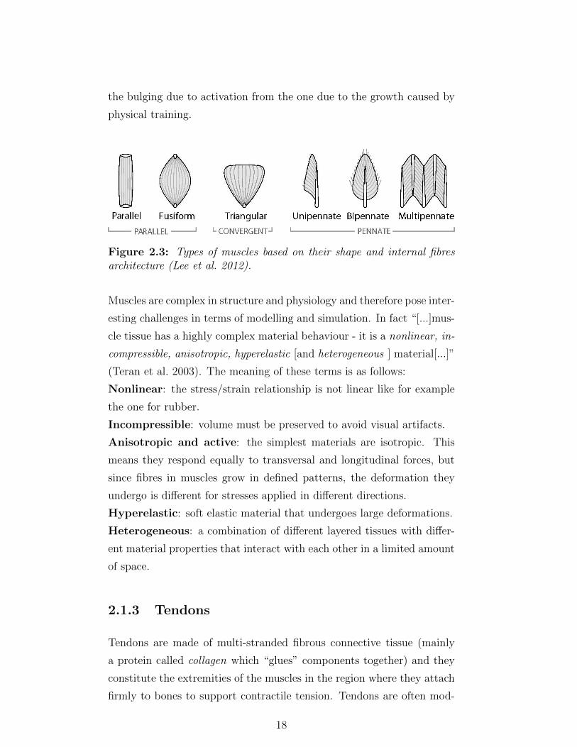
Muscles present various configurations of fibres and internal architec-
tures, based on their shape (Figure 2.3). For example, the gluteus max-
imum has a pennate architecture while the bicep brachii has a fusiform
one. These characteristics must be taken into account in a simulation
system.
When activated, muscles bulge and their shape depends on the rest pose
configuration (i.e. the initial vertex position prior to any deformation),
the fibre density, their internal fibre architecture and the fact that they
interact with the surrounding muscles and fascia. Bodybuilders know
very well that the range and kind of exercises for specific muscles in-
fluence determined fibre areas. For instance, bicep curls that are more
or less extended (in terms of arm angle) can shape the bicep brachii
differently because different fibre groups are exercised (broken and re-
paired) (Siegel, Jeffrey 2015). Moreover, it is important to distinguish
17
the bulging due to activation from the one due to the growth caused by
physical training.
Figure 2.3: Types of muscles based on their shape and internal fibresarchitecture (Lee et al. 2012).
Muscles are complex in structure and physiology and therefore pose inter-
esting challenges in terms of modelling and simulation. In fact “[...]mus-
cle tissue has a highly complex material behaviour - it is a nonlinear, in-
compressible, anisotropic, hyperelastic [and heterogeneous ] material[...]”
(Teran et al. 2003). The meaning of these terms is as follows:
Nonlinear: the stress/strain relationship is not linear like for example
the one for rubber.
Incompressible: volume must be preserved to avoid visual artifacts.
Anisotropic and active: the simplest materials are isotropic. This
means they respond equally to transversal and longitudinal forces, but
since fibres in muscles grow in defined patterns, the deformation they
undergo is different for stresses applied in different directions.
Hyperelastic: soft elastic material that undergoes large deformations.
Heterogeneous: a combination of different layered tissues with differ-
ent material properties that interact with each other in a limited amount
of space.
2.1.3 Tendons
Tendons are made of multi-stranded fibrous connective tissue (mainly
a protein called collagen which “glues” components together) and they
constitute the extremities of the muscles in the region where they attach
firmly to bones to support contractile tension. Tendons are often mod-
18

elled as completely inextensible, but they are actually flexible and stiff at
the same time. In fact their elastic properties are important not only for
transmitting forces to the bones and allowing the muscles to bulge, but
in some cases they behave like springs to store and release energy during
motion for efficiency (like the Achille’s tendon during the stride). The
Hill-type model (Zajac 1989a) takes this behaviour into consideration.
Tendons are visible on the skin in particular in superficial areas of the
hand, wrist and foot where they can be seen sliding and convey overall
sense of tension.
2.1.4 Fascia
Figure 2.4: Fascia at work c© (Fortier 2013).
Fascia is an extremely important component of the musculo-skeletal sys-
tem. In a broad sense it is the soft tissue webbing of the body. It can
take the form of sheets, but in general is a 3D network of connective tis-
sue. Its main function is to hold muscles, organs and other components
together. Without fascia our body parts would literally fall apart. Fas-
cia connects muscles to other muscles. The fibres constituting the fascia
keep forming and breaking all the time, but with lack of movement tend
to make the muscles stick together too much (a process called adhesion)
and create dragging forces one on another, something that reduces the
natural sliding and augments friction (Stecco 2012)
Keeping in mind that fascia is a global system, it can be subdivided
for simplicity into superficial and deep. Superficial fascia is the layer of
viscoelastic subcutaneus loose connective tissue that mainly determines
19
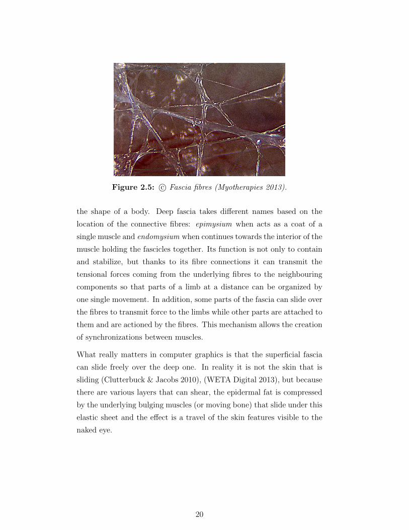
Figure 2.5: c© Fascia fibres (Myotherapies 2013).
the shape of a body. Deep fascia takes different names based on the
location of the connective fibres: epimysium when acts as a coat of a
single muscle and endomysium when continues towards the interior of the
muscle holding the fascicles together. Its function is not only to contain
and stabilize, but thanks to its fibre connections it can transmit the
tensional forces coming from the underlying fibres to the neighbouring
components so that parts of a limb at a distance can be organized by
one single movement. In addition, some parts of the fascia can slide over
the fibres to transmit force to the limbs while other parts are attached to
them and are actioned by the fibres. This mechanism allows the creation
of synchronizations between muscles.
What really matters in computer graphics is that the superficial fascia
can slide freely over the deep one. In reality it is not the skin that is
sliding (Clutterbuck & Jacobs 2010), (WETA Digital 2013), but because
there are various layers that can shear, the epidermal fat is compressed
by the underlying bulging muscles (or moving bone) that slide under this
elastic sheet and the effect is a travel of the skin features visible to the
naked eye.
20

2.1.5 Fat
Between the fascia and the epidermis (skin) there is a more or less thick
layer of adipose tissue. It is present almost everywhere on the body but
it accumulates more in certain areas, typically the belly, the arm and
the gluteal region. While the muscles mainly give the basic deformation
and silhouette of a character, it is the fat layer which gives most of the
interesting secondary effects such as jiggling, wave propagation due to
impact and sense of inertia.
2.1.6 Skin
Skin can be approximated as an elastic sheet that can wrinkle under
compression of the underlying tissues. When stretched it tends to return
to its original configuration with a nonlinear delay. Skin is of primary
importance in computer graphics because, except for particular cases
where seeing the underlying anatomical geometry is needed, it is the
layer that is visible and renderable.
2.1.7 Veins
Veins form an indispensable network for the circulatory system. In
graphics, even if often neglected, they are particularly important to con-
vey realism. In fact veins are always visible and they stand out not
only for their blueish colour, but also for their displacement. When
muscles contract and undergo a medium-high effort, veins become more
pronounced for the larger amount of blood that flows in and out the
fibres and the higher pressure. For this reason they should be taken into
account for maximum realism.
21
2.2 Muscle systems background
In the VFX pipeline, at the stage of muscle simulation, rigging starts
to blend with character FX: the anatomical tissues have to be combined
into layers and be simulated in each shot. For that purpose, muscles
are first constrained to the bone geometry at their attachment points
(proximal and distal insertions of the tendons) and to each other with
a combination of hard, soft and sliding constraints. A non-volumetric
geometry component is then procedurally generated from the outline of
the bones and muscles: it wraps them tightly and that functions as the
anatomical fascia. The fascia is responsible for holding the deforming
muscles together and forming a clear separation from the volumetric
outer layer that constitutes the fat directly attached to the renderable
skin. All these layers interact with each other and are (ideally) simulated
all at once to obtain physics coupling. This is computationally expensive
so a common strategy is to simulate the layers separately generating a
geometry cache for each to drive the next. Despite being more flexi-
ble, the drawback of this approach is that it cannot obtain a physically
and visually correct coupling or bidirectional transfer of inertia during
animation (Jacobs et al. 2016). By placing constraints and specifying
correct material properties (Young’s modulus, Poisson ratio, stiffness),
the solver of choice will compute forces, stresses, contacts and collisions.
The result is an anatomical mesh that follows the animation of the char-
acter, but is enriched with fibre activations, muscle and bones sliding
under the fat, skin wrinkles and jiggling effects which add that level of
realism highly sought after and appreciated in Visual Effects. In real
productions, the process described above is highly nonlinear and heavily
iterative.
As mentioned earlier this approach is not free from problems that have
to be carefully considered. For example given the effort needed to obtain
the anatomical muscles for a character, transferring algorithms have to
be developed and practical tools given to artist when, for production
reasons, the skin and proportions of the character have to be changed.
Similarly, when for a shot the muscle and fat simulations result in shapes
22

that are anatomically correct but do not convey the director’s creative
intention, shapes have to be corrected and coexist with the simulation
pipeline. These kind of situations are the “bread and butter” of everyday
VFX movie production.
While muscle systems are generally intended for the body, research is ad-
vancing their use for facial animation, an area where simulation is being
adopted especially for blend shape-based tetrahedral rigs (Kozlov et al.
(2017), Ichim et al. (2017)). Facial muscle systems are more challenging
than the body ones because detailed facial expressions require extreme
amount of detail (i.e. wrinkles), high levels of controllability are diffi-
cult to be provided and also because the face contains very thin muscles
which pose problems for the solvers.
Specifically at MPC riggers take care of the generation of the muscle ge-
ometry, via a custom procedural system that from 2D morphable sheets
skinned to the joints generates an approximation of muscle anatomical
shapes (Fig. 2.6). After controlling that the character deforms correctly,
a mass-spring system adds approximated dynamics to the muscles which
are connected to the skin via a custom skin deformer that roughly be-
haves like a highly controllable quasi-static cloth simulation, producing
secondary effects such as wrinkles. Because of the lack of fibre-based
mesh contraction, the rig is equipped with “sensors” of compression and
extension based on joint angles and impact zones that activate custom
sculpted blend shapes (flex-shapes). While this solution is very art-
directable, Rigging and Techanim needed a system that produced more
physically-based realistic results which constitutes one of the motivations
behind the proposed methods and tools described in this work.
2.3 Solvers and Methods for Deformable
Objects
Muscle systems are modelled as deformable objects. Here some back-
ground and mathematics for deformable objects will be presented.
23

Figure 2.6: Front, back and side muscles of arm and torso (MPC mus-cles generated from anatomical sheets).
To give some initial basic definitions, the deformation of a mesh element
(i.e. triangle or tetrahedron) expressed as a vector of vertex positions in
rest pose X to a deformed configuration x can be defined by a function
Φ(x). The Jacobian of this function constitutes a basic description of the
severity of the deformation (variation with respect to the rest pose) and
it is called the deformation gradient, widely indicated in the literature
as F.
A physics solver’s task is to provide at each timestep a solution to the
partial differential equation of motion:
Ma +∇xW(X,x) = fext (2.1)
where M is the mass matrix, a is the acceleration, fext are the external
forces (gravity, wind, constraints, contact forces) and W is an elastic
potential that typically expresses the kind of material to be simulated.
Different materials have different properties: in this work we will focus on
hyperelastic materials and in particular the St Venant-Kirchhoff (StVK)
invertible model (Bonet & Wood 1997).
There are mainly two ways to solve this equation in time for a deformable
object:
1. Using an integration scheme for the PDE and solving the resulting
nonlinear system
2. Transforming 1. into an equivalent energy minimization problem
The first approach integrates the discretized differential equations of mo-
24

tion by solving a nonlinear system for which the solution is the velocity
at the next state. The most stable and popular way to do this is us-
ing Implicit Backward Euler integration. Given the state of the system
(qn, vn) at time n, Implicit Euler adopts the following update rule:
qn+1 = qn + hvn+1
vn+1 = vn + hM−1(fint(qn+1) + fext)
where h is the time step size (discretization of time). The fully implicit
nonlinear equation therefore becomes:
M(qn+1 − qn − hvn) = h2(fint(qn+1 + fext))
As will be shown in chapter 4, the solver used in this work instead adopts
a semi-implicit integration scheme, that linearizes fint through its gra-
dient with respect to the nodal positions which is called the tangent
stiffness matrix K.
The second approach is to express the Implicit Euler integration as a
minimization problem and therefore takes advantage of a long tradition
of research in the mathematical optimization field:
minqn+1
1
2h2‖M
12 (qn+1 − qn − hvn − h2M−1fext)‖2F +
∑i
Wi(qn+1)
which expresses the fact that the solution (positions at time n + 1) is a
compromise between the momentum potential plus external forces (first
term) and the total elastic potential (second term). Chapter 7 shows
that this potential can become a suitable loss function for a machine
learning algorithm.
The resulting nonlinear system of equations is generally solved with one
or more iterations of the Newton-Raphson method. The linearization of
25

the equation via the Newton procedure leads to a sparse positive definite
linear system that can be solved with a Preconditioned Conjugate Gra-
dient (PCG) solver or direct solvers (Sifakis & Barbic 2012). Existing
work on solvers and methods for deformable objects is presented below,
divided for convenience into four macro categories: offline, interactive,
procedural and machine-learning based methods.
2.3.1 Offline Physics-Based Methods
Deformable models have been studied in computer graphics for nearly
30 years now, starting with seminal works (Terzopoulos et al. (1987),
Terzopoulos & Fleischer (1988)) which showed the potential of computa-
tional physics to simulate fracture, deformation, viscoelasticity and plas-
ticity using mainly a finite differences discretization. To deal with large
deformations, O’Brien & Hodgins (1999) and O’Brien (2002)) used a
St.Venant-Kirchhoff (StVK) nonlinear material model based on quadratic
Green strain. Muller & Gross (2004) contributed to solve the prob-
lem of linear elasticity artifacts for large deformations by introducing in
the framework of the Finite Element Method (FEM) (Sifakis & Barbic
2012), (Bonet & Wood 1997) the popular corotational method (warped
stiffness) that extracts the rotation of the deformation gradient F via po-
lar decomposition (alternatively, QR decomposition). In fact rotational
modes have to be filtered out so that they do not contribute to internal
forces. Volume preservation was addressed in (Irving et al. 2007).
The coupling of computer graphics with biomechanics in recent years has
led to a more anatomically “conscious” approach to character animation.
The underlying assumption of the following methods is that an accurate
geometry representation of the internal anatomical components, coupled
with physics-based simulation, gives the most realistic results. Teran
et al. (2005b) and Teran et al. (2003)) simulate muscles and flesh from
the Visible Human data set using a variation of classic FEM, the Finite
Volume Method, supporting: active and passive components (tendons),
an effective constitutive model based on fibres and degenerate and in-
verted tetrahedra (via SVD decomposition that diagonalizes F (Irving
26
et al. 2004)). After these works had shown the approach as being very
promising, other researchers concentrated on the physics-based simula-
tion of the human hand (Sueda et al. 2008), the upper body (Lee et al.
2009) and human swimming coupled with fluid dynamics using Lattice
Deformers (Si et al. 2014), (Patterson et al. 2012).
Forces in elementary muscle units (sarcomers) have been represented
classically through the Hill-Zajac model (Zajac 1989b) which is an ac-
ceptable 1D simplification of the macroscopic forces. Biomechanics started
relatively recently to adopt 3D muscle simulation (Blemker & Delp 2005),
to predict shapes during contraction and internal stresses to prevent in-
juries in a much more accurate way than before (Comas et al. 2008),
(Delp et al. 2007). Non-volumetric muscles are also used for control of
animation, often in conjunction with quadratic programming techniques
to resolve contacts (Tan et al. 2012), (Geijtenbeek et al. 2013)
The price to pay to have accuracy is quite high in computational terms
and methods to trade speed for physical correctness are an area of active
research. In fact typical full body models can easily reach 1 million
tetrahedral elements. Moreover such biomechanical systems are difficult
to model, setup and control without dedicated tools which generally are
very different from the ones present in traditional Visual Effects rigging
pipelines.
Recently, McAdams et al. (2011) created a production-ready system
for the deformation with contacts of characters that works both quasi-
statically and with dynamics. Using a conforming hexahedral lattice
built from the mesh, the method corrects the indefiniteness of the stiff-
ness matrix to fix instabilities of the warped stiffness method and makes
use of a fast multigrid solver which achieves near-interactive performance.
A new approach to deformation that is inspired by fluid dynamics meth-
ods is Eulerian Solids in which deformable objects are simulated on a
grid through material coordinates mapping and advection (Levin et al.
2011). Its advantages are that it handles collisions well, preserves volume
in large deformations and does not need remeshing to avoid instabilities
(something needed for Lagrangian methods, subject to mesh tangling).
27

The method has been applied successfully to muscles simulation (Fan
et al. 2014) and its extension, called Eulerian-on-Lagrangian method,
allows the simulation of skin sliding (Li et al. 2013) and tendon biome-
chanics (Sachdeva et al. 2015). Some of the drawbacks are that an ex-
plicit mesh has to be mapped and there is no current implementation of
internal fibres.
Not only the body but also the face has been the object of study in terms
of achieving more realistic dynamics. Kozlov et al. (2017) enrich blend
shape animations with secondary motion and other physical effects with
a FEM simulation based on the minimization framework by Martin et al.
(2011). The method utilizes volumetric blend shapes and per-frame rest
poses to guarantee fidelity to the artist’s animation.
Ichim et al. (2017) embed simple muscle geometries in a tetrahedral mesh
of the face dividing the tetrahedra (tets) that are passive from the active
ones and attaching the mesh to the skull with pin and sliding constraints
controlled by a map. Muscle activations are obtained from the blend
shape animation solving an inverse problem and the muscle model is
translation and rotation invariant. Simulation is done by minimizing a
set of non-linear potential energies using an interior point solver.
In terms of artistic control of these simulations, Martin et al. (2011)
propose an example-based approach where an artist can sculpt a set of
target shapes which are interpolated during a physical simulation very
smoothly. Each example acts as an additional elastic force but with-
out introducing visible spurious violation of energy conservation. This
art-directable way of controlling the simulation avoids tedious parame-
ter tweaking and was extended by Schumacher et al. (2012) to support
plasticity and application to a bending muscular arm using pose based
dynamics. The development of these methods is fundamental in the
context of musculo-skeletal simulation.
Even though all these works achieve stunning results, there are still gaps
in the literature for papers that perform dynamic simulation of the com-
bination of all the layers and showing realistic results on the renderable
skin of tendons, wrinkles, fascia, self collisions etc.
28
2.3.2 Interactive and Real-Time Methods
Videogames and interactive applications require new methods to simu-
late deformable objects at real-time and near-real-time rates. For this
purpose the simplest approaches use tetrahedral springs (Mollemans
et al. 2003). Muller et al. (2005) introduced the shape matching tech-
nique, a mesh-free method that is particularly suited for real time ap-
plications and produces plausible deformations although its accuracy is
limited by not being physically-based. Kim & Pollard (2011) achieve
interactive rates for skeleton-driven non-linear deformation of charac-
ters through clever optimizations and parallelizations. Careful algorith-
mic solutions, often aiming at exploiting GPU architectures, lead to so-
phisticated real-time surgical simulators and efficient muscle simulation
(Mitchell et al. 2015). Model reduction techniques (Barbic & James
2005) aim at expressing deformations as combination of displacement
fields (modes).
Position Based Dynamics (PBD) (Muller et al. 2007) is a method that
operates directly on the positions of the nodes. In a first step positions
are guessed using explicit integration and then validated/corrected by
applying distance, bending, volume and collision constraints. Upon val-
idation these values are integrated to new positions. Although it comes
at the price of reduced accuracy, this has several advantages: it is easy
to implement; it is very controllable; vertex positions can be directly
manipulated in real time; constraints and collisions are handled quite
easily. The limitations of PBD, in particular the constraint stiffness de-
pending on time step and iteration count, have been addressed recently
in the work by Macklin et al. (2016). XPBD extends its predecessor
by formulating the constraints in a way that has correspondence with
elastic energy potentials and by using total Lagrange multipliers. The
result is a fast and stable solver that supports arbitrary elastic potentials
(materials).
Recently, Projective Dynamics (Bouaziz et al. 2014), extending the work
on fast mass springs by Liu et al. (2013), introduced a new solver that
combines FEM with PBD. The solver treats elastic potentials as projec-
29

tions of position configurations on a constraint manifold. This results in a
particular form of the potential energy that is minimized via local/global
alternated solves. It also supports a wide variety of energy-based con-
straints.
Projective Dynamics limitations have also been overcome in the work
by Liu et al. (2017) by considering it as a quasi-Newton method which
allows it to simulate any hyperelasic material and be 10 times faster than
one iteration of Newton’s method.
Saito et al. (2015) propose a method, built on the Projective Dynamics
solver, to simulate the biological growth processes of muscles and fat
on a volumetric model. They achieve this by initially decomposing the
deformation gradient in growth and elastic components and crafting an
ad-hoc potential energy. Even if the results achieved are remarkable
and the technique interactive, the system does not cover the possibility
for the growth process to fit an existing target mesh, something highly
desirable in Visual Effects.
2.3.3 Procedural Methods
Skinning refers to a general class of procedural techniques which are very
computationally efficient and commonly used to obtain fast deformations
of skeleton-based characters. Geometric/Procedural skinning techniques
have been developed in computer graphics for a long time. Shape inter-
polation and example-based approaches (Lewis et al. 2000), (Sloan et al.
2001) are used in the industry on a daily basis (called blend shapes)
while Linear Blend skinning (Magnenat-Thalmann et al. 1988) and dual
quaternion (Kavan et al. 2008) have well known issues such as loss of
volume or excessive bulging at joints. Jacobson et al. (2011) calculate
bounded biharmonic weights for 2D and 3D objects by Laplacian energy
minimization subject to bound constraints in a shape-aware, localized
manner and with the use of quadratic programming.
More recently Vaillant et al. (2013) proposed the Implicit Skinning with
contact technique, followed by its improvement to support skin elasticity
30

with convincing results (Vaillant et al. 2014). These methods have the
advantage of being fast, but they generally fail in robustly handling self
and external collisions, volume preservation and nonlinear deformations,
in addition to the fact that dynamics are often faked.
Deformers are important tools used in the visual effects industry on a day
to day basis, especially in Rigging. One of such widely used deformers is
the Free Form Deformation technique (Sederberg & Parry 1986), which
uses a cubic lattice grid of points to intuitively edit the shape of an
embedded mesh. Another popular method to edit shapes is the Laplacian
deformer (Sorkine et al. 2004), which has the advantage of preserving well
geometric details.
Procedurality and automatisms are also important for transferring of
shapes from one character to another. Ali-Hamadi et al. (2013) create a
system that can transfer volumetric anatomical models across different
target shapes using harmonic energy minimization (Laplacian interpo-
lation) and anatomy rules as constraints. Cong et al. (2015) present a
morphing algorithm to transfer anatomy including muscles across faces
of different characters, based on feature points and feature curves corre-
spondences.
2.3.4 Methods based on acquisition and machine
learning
In recent years other ways to deal with deformable object have been
developed. In particular the application of techniques from other areas
of Computer Science, such as machine learning and other statistical-
based approaches from Artificial Intelligence, have started to become
increasingly popular.
Sifakis et al. (2005) acquire activation levels for a volumetric muscle
based facial system from sparse marker data. SCAPE (Anguelov et al.
2005) learns from several body scans of people and creates a model de-
pendent on both body shape and pose of the articulated skeleton. Bickel
et al. (2009) create a deformable model of heterogeneus materials by
31

finding material parameters given force and strain sample measurements
as inputs. Neumann et al. (2013) model the statistical variations of
fine scale muscle deformations from reconstructed surfaces of a subject’s
arms. Their model also supports force application which expresses iso-
metric contraction effects. Zhu et al. (2015) learn anthropometric pa-
rameters from point cloud data of a subject’s arm acquired with depth
sensors and matches a deformed anatomical model containing bones and
skinning (but no muscles). DYNA (Pons-Moll et al. 2015) in addition
to SCAPE predicts soft-tissue deformations by learning a second-order
auto-regressive model based on 40000 scans of 10 subjects.
Data-driven models have become very advanced in recent years. How-
ever, in general they can suffer from incomplete input data (due to occlu-
sion) or can be not robust when parameters go far beyond the range the
system was trained for. In Visual Effects it is common to have charac-
ters performing highly risky actions or movements which are not realistic
to acquire and can be very dissimilar from the training set. Moreover
there are gaps in the research regarding highly controllable deformation
models (at the vertex level).
Machine Learning, and in particular Deep Learning, have been applied
recently to the learning of physical models and in particular fluid simu-
lation. Tompson et al. (2016) obtain very convincing results for smoke
simulations using a tailored Deep Neural Network operating on a vol-
umetric grid. The system, unsupervised, is trained to approximate the
solution of the linear system to compute the pressure equation, minimiz-
ing the divergence of the velocity field. Ladicky et al. (2015) also use a
data-driven approach to learn fluid dynamics but adopt regression forests
in a supervised manner for the regression of acceleration of particles at
a given time step.
Table 2.1 provides a qualitative comparison of most of the main methods
in the literature and puts in evidence their advantages and disadvantages.
Table 2.1: Comparison of deformable objects methods
METHOD PROs CONs
32
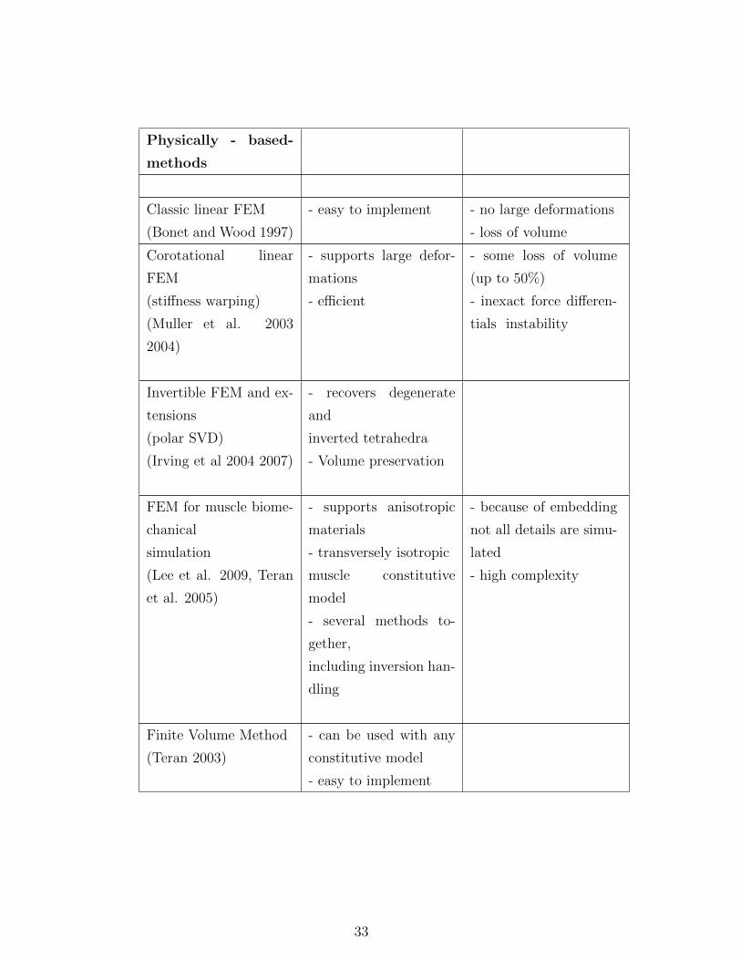
Physically - based-
methods
Classic linear FEM
(Bonet and Wood 1997)
- easy to implement - no large deformations
- loss of volume
Corotational linear
FEM
(stiffness warping)
(Muller et al. 2003
2004)
- supports large defor-
mations
- efficient
- some loss of volume
(up to 50%)
- inexact force differen-
tials instability
Invertible FEM and ex-
tensions
(polar SVD)
(Irving et al 2004 2007)
- recovers degenerate
and
inverted tetrahedra
- Volume preservation
FEM for muscle biome-
chanical
simulation
(Lee et al. 2009, Teran
et al. 2005)
- supports anisotropic
materials
- transversely isotropic
muscle constitutive
model
- several methods to-
gether,
including inversion han-
dling
- because of embedding
not all details are simu-
lated
- high complexity
Finite Volume Method
(Teran 2003)
- can be used with any
constitutive model
- easy to implement
33
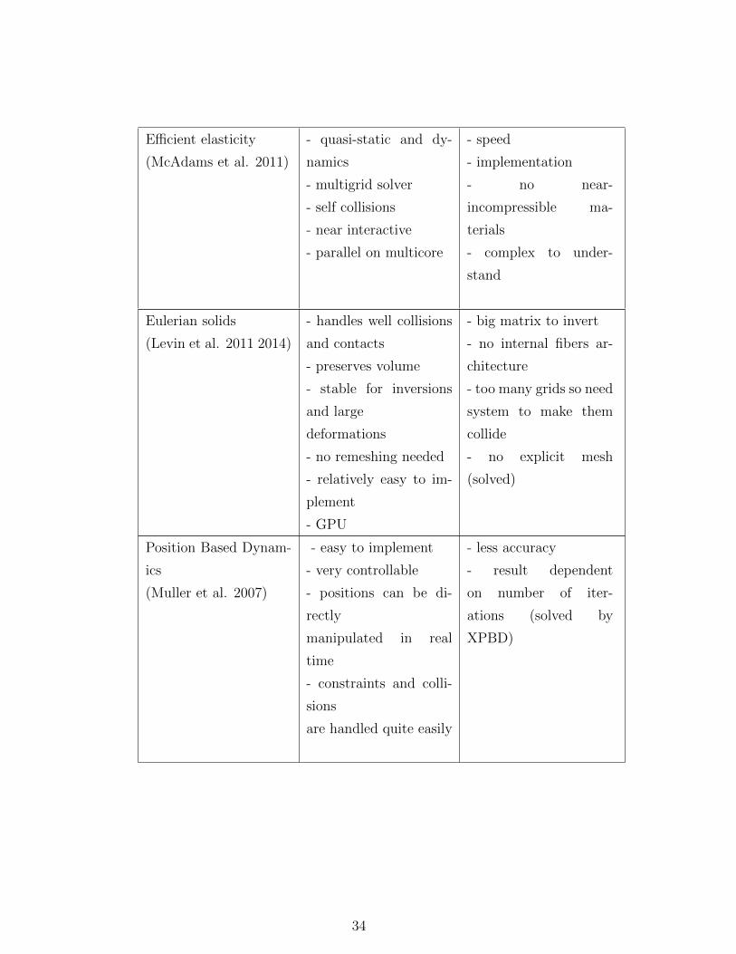
Efficient elasticity
(McAdams et al. 2011)
- quasi-static and dy-
namics
- multigrid solver
- self collisions
- near interactive
- parallel on multicore
- speed
- implementation
- no near-
incompressible ma-
terials
- complex to under-
stand
Eulerian solids
(Levin et al. 2011 2014)
- handles well collisions
and contacts
- preserves volume
- stable for inversions
and large
deformations
- no remeshing needed
- relatively easy to im-
plement
- GPU
- big matrix to invert
- no internal fibers ar-
chitecture
- too many grids so need
system to make them
collide
- no explicit mesh
(solved)
Position Based Dynam-
ics
(Muller et al. 2007)
- easy to implement
- very controllable
- positions can be di-
rectly
manipulated in real
time
- constraints and colli-
sions
are handled quite easily
- less accuracy
- result dependent
on number of iter-
ations (solved by
XPBD)
34

Lattice deformers
(Patterson et al. 2012)
- regular structure
optimization
- no need for a mesh per
muscle
- accurate volume
preservation with gen-
eral
treatment of incom-
pressibility
- quasi-static and dy-
namics
- some voxelization arti-
facts are noticeable
- complex to under-
stand
- no collision treatment
(yet)
- small scale topology
- no direct manipulation
of mesh
Procedural / Geo-
metric methods
Linear Blend skinning
(Magnenat-Thalmann
et al. 1988)
- fast
- no collisions
- loss of volume
- candy wrap effect
Dual Quaternion skin-
ning
(Kavan et al. 2008)
- fast
- no collisions
- bulge at joints
Steklov-Poincare skin-
ning
(Gao et al. 2014)
- interactive
- physically based
- supports collisions
- pose dependent, no
need to
correct indefiniteness of
stiffness matrix
- quasistatic only (pos-
sible extension)
- probably not suitable
for deep and strong con-
tacts
- not implicit time inte-
gration (yet)
35
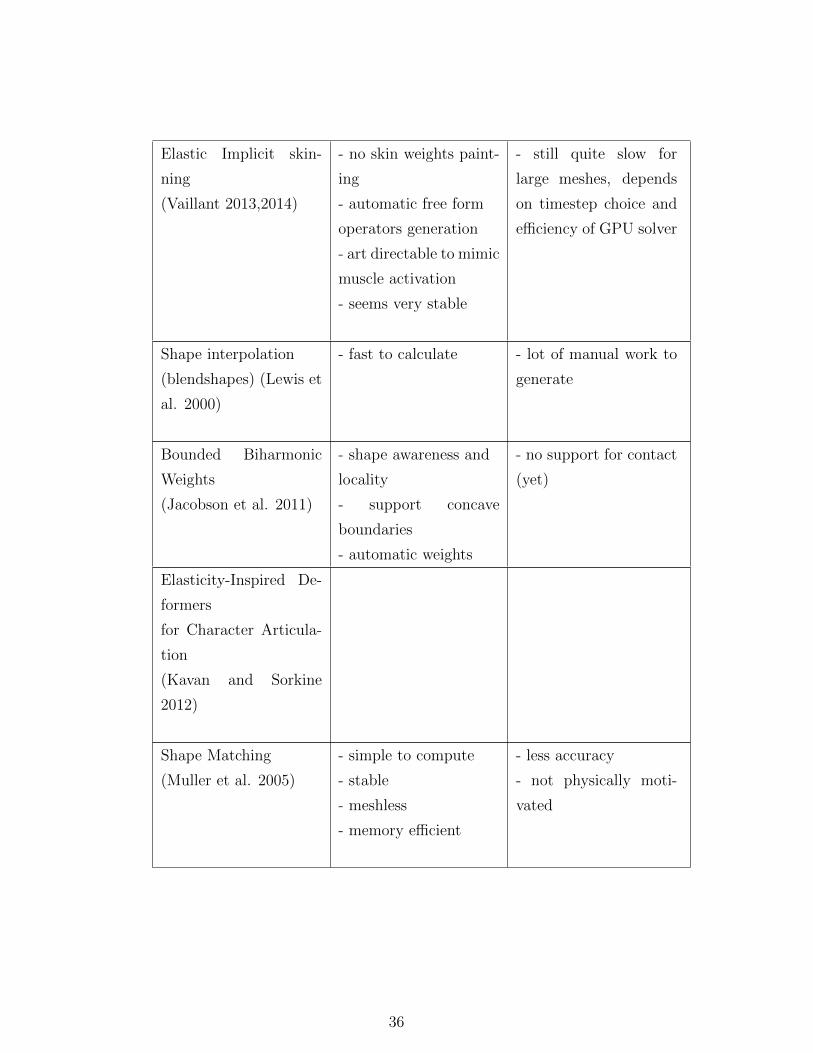
Elastic Implicit skin-
ning
(Vaillant 2013,2014)
- no skin weights paint-
ing
- automatic free form
operators generation
- art directable to mimic
muscle activation
- seems very stable
- still quite slow for
large meshes, depends
on timestep choice and
efficiency of GPU solver
Shape interpolation
(blendshapes) (Lewis et
al. 2000)
- fast to calculate - lot of manual work to
generate
Bounded Biharmonic
Weights
(Jacobson et al. 2011)
- shape awareness and
locality
- support concave
boundaries
- automatic weights
- no support for contact
(yet)
Elasticity-Inspired De-
formers
for Character Articula-
tion
(Kavan and Sorkine
2012)
Shape Matching
(Muller et al. 2005)
- simple to compute
- stable
- meshless
- memory efficient
- less accuracy
- not physically moti-
vated
36
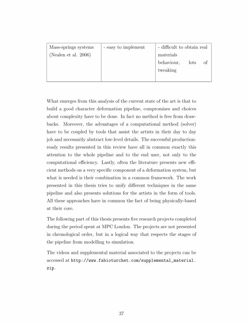
Mass-springs systems
(Nealen et al. 2006)
- easy to implement - difficult to obtain real
materials
behaviour, lots of
tweaking
What emerges from this analysis of the current state of the art is that to
build a good character deformation pipeline, compromises and choices
about complexity have to be done. In fact no method is free from draw-
backs. Moreover, the advantages of a computational method (solver)
have to be coupled by tools that assist the artists in their day to day
job and necessarily abstract low-level details. The successful production-
ready results presented in this review have all in common exactly this
attention to the whole pipeline and to the end user, not only to the
computational efficiency. Lastly, often the literature presents new effi-
cient methods on a very specific component of a deformation system, but
what is needed is their combination in a common framework. The work
presented in this thesis tries to unify different techniques in the same
pipeline and also presents solutions for the artists in the form of tools.
All these approaches have in common the fact of being physically-based
at their core.
The following part of this thesis presents five research projects completed
during the period spent at MPC London. The projects are not presented
in chronological order, but in a logical way that respects the stages of
the pipeline from modelling to simulation.
The videos and supplemental material associated to the projects can be
accessed at http://www.fabioturchet.com/supplemental_material.
zip.
37

Part II
Projects
38
Chapter 3
Muscle Modelling
3.1 Introduction
In recent years, physics-based muscle simulation has become increasingly
popular in the Animation and Visual Effects industry. Examples of ex-
cellent Research and Development from companies which was applied to
specific movie productions include the FEM Tissue System at Weta Dig-
ital (WETA Digital 2013), PhysBam-based Zeno at ILM (Comer et al.
2015), the PhysGrid-based system at Disney (Milne et al. 2016) and the
interactive system for skin sliding at Method Studios based on ADMM
and Projective Dynamics (Saito & Yuen 2017). This work takes inspira-
tion also from those results.
The muscle system which is used for these purposes usually contains the
following components:
• Anatomically correct muscle geometries;
• A fibre field defined on them;
• A constitutive model supporting fibre activation for contraction;
• A skeleton model on which the muscles attach via constraints;
• A physics solver that computes the dynamics of the system.
This chapter focuses on the first component of the list. In fact one of
39
the most time-consuming steps of a character simulation pipeline is the
initial setup of the input model.
Muscle geometries can be generated in various ways: sculpted per-character
by trained artists, created from MRI and CAT scan data as in Jacobs
et al. (2016), or transferred from an existing template. However, the
sculpting process is time-consuming because it requires ad-hoc work for
each character, the data scans are not always available and the fitting
of templates to new characters presents challenges when dealing with
non-humanoid or fantastic creatures which have atypical features, body
proportions and body mass distribution. Moreover the result is gen-
erally not simulation-ready because of the interpenetrations present in
the input meshes, i.e. intersections of various mesh objects representing
different muscles.
In this work the complexity of the sculpting process is reduced by in-
troducing methods that allow artists to create volumetric muscle shapes
complete with tendons from sketches of muscle silhouettes (patches) de-
fined on the external surface of a character (skin) and attachment points
corresponding to the insertion and origin of anatomical muscles on the
skeleton. By using an artist-led physically-based simulation framework
that includes shape inflation in the direction of the skeleton and muscle-
to-muscle and muscle-to-bone collision handling, a user can design plau-
sible volumetric reconstructions. As a result the shape of the muscle and
the corresponding fibre field are obtained, both ready for further simu-
lations. The key idea of the system is to exploit the information of the
sculpted or scanned skin of a character such as detailed areas (patches)
that correspond to superficial muscles and use them to generate plausible
volumetric reconstructions which are interpenetration-free. The results
obtained show how using these patches can reduce the complexity of the
sculpting process, while guaranteeing that output meshes are suitable for
simulation.
40

Figure 3.1: A slice of the arm muscle primitives showing intricate in-tersections.
3.1.1 Muscle Primitives fixing
One of the motivations behind research in muscle modelling is that at
the beginning of the exploration for solutions at MPC, a very accurate
anatomical model was not available. The belief was that fixing the primi-
tives (shown in Figure 2.6) of the existing rigging system would have been
enough to create simulation-ready volumes. The intersections severity to
be fixed varied from superficial to deep (Figure 3.1).
However, the assumption was not entirely correct as it became very hard
or even impossible to fix (i.e. to free from intersections) all the muscles
in the general case. The small and medium cases were successfully fixed
by converting geometry to signed distance fields and using interactive
marching of the vertices in the normal direction, a method similar to
implicit skinning described in more detail in chapter 6. An example
of successful muscle fixing is shown in Figure 3.2. However for deep
intersections, for example when meshes of small muscles were completely
inside meshes of other muscles, automatic fixing was not possible.
Another solution to the problem of fixing primitives could be apply-
ing physical-based approaches. Geometries could for example be moved
apart from each other like in an exploded view and then animated back
41

(a) (b)
(c)
Figure 3.2: (a) intersecting geometries of the forearm; (b) solved inter-sections, (c) highlighted fixed areas.
to their original positions solving for collisions quasi-statically when they
occur. Just like the case of the wrong projections problem in Implicit
Skinning solved in Vaillant et al. (2014), the solution would thus emerge
by taking advantage of the time variable. It should be noted that the
problem of fixing intersecting geometries can be avoided if riggers are pro-
vided with tools to model muscles interactively with the help of physics:
this chapter explores exactly that direction.
42

3.2 Related Work
Previous research work containing methods to produce muscle primitives
relies mainly on existing anatomical data. Teran et al. (2005a) create
tetrahedral meshes from the Visible Human dataset via level sets and are
able to reconstruct missing tendon information using Constructive Solid
Geometry. More recently, the work by Jacobs et al. (2016) reconstructs
very accurate musculature of a full body female subject via segmented
cross sectional MRI data for simulation purposes. Saito et al. (2015) in-
stead utilize a commercially available anatomical model and focus on the
physics-based modelling of different body shapes by growing or shrink-
ing muscles and fat. In a production setting such as at MPC, because
of the complexity of modelling muscles, a popular way to create them is
by using either parametric surfaces or procedural primitives controllable
with numerous parameters.
The fibre field in Teran et al. (2005a) is obtained with B-spline solids and
used to simulate muscle contraction with the Finite Elements Method
and a transversely isotropic constitutive model, while the more recent
work of Choi & Blemker (2013) focuses on obtaining the fibre field by
solving a Laplace equation subject to flux boundary conditions in the
tendon regions.
Following the popularity gained by muscle systems in recent years, re-
searchers also started to focus on the problem of transferring anatomical
templates between characters. Previous work (Sumner & Popovic 2004)
focused mainly on registration and deformation transfer of superficial
meshes, but not of internal information except for the skeleton. However,
the transfer of complex internal anatomical structures require ad-hoc so-
lutions. The works by (Ali-Hamadi et al. 2013) for the body and by
(Cong et al. 2015) for the face fill this gap by transferring procedurally
complex template models across similar characters, with the possibility
of affecting the result with artist input. These solutions speed up char-
acter production, but in some cases can produce unwanted deformations
when source and target shapes are substantially different. The inspi-
ration for the work in this Chapter came by the field of computational
43
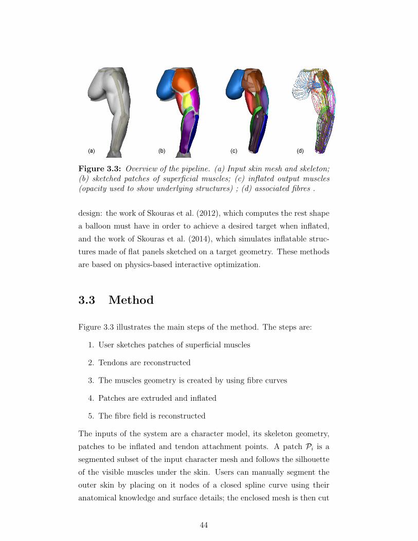
Figure 3.3: Overview of the pipeline. (a) Input skin mesh and skeleton;(b) sketched patches of superficial muscles; (c) inflated output muscles(opacity used to show underlying structures) ; (d) associated fibres .
design: the work of Skouras et al. (2012), which computes the rest shape
a balloon must have in order to achieve a desired target when inflated,
and the work of Skouras et al. (2014), which simulates inflatable struc-
tures made of flat panels sketched on a target geometry. These methods
are based on physics-based interactive optimization.
3.3 Method
Figure 3.3 illustrates the main steps of the method. The steps are:
1. User sketches patches of superficial muscles
2. Tendons are reconstructed
3. The muscles geometry is created by using fibre curves
4. Patches are extruded and inflated
5. The fibre field is reconstructed
The inputs of the system are a character model, its skeleton geometry,
patches to be inflated and tendon attachment points. A patch Pi is a
segmented subset of the input character mesh and follows the silhouette
of the visible muscles under the skin. Users can manually segment the
outer skin by placing on it nodes of a closed spline curve using their
anatomical knowledge and surface details; the enclosed mesh is then cut
44

and extracted (see Fig. 3.3b). For each muscle that a patch represents,
attachment points are positions on the input skeleton where its tendons
attach (see section 3.3.2). This approach has limitations when the skin
of the character doesn’t present clear enough anatomical features of the
muscles. This happens for example when the adipose tissue (fat) smooths
out the details and tends to flatten out the curvature on the skin. In
these cases the application of the method is still possible, but does not
necessarily produce organic shapes of the muscles. However, the ad-
vantage of sketching the input patches from the surface guarantees that
there is a clear separation between the muscles at the superficial level,
while the internal non-intersection is guaranteed by the tendon creation
rules first (collision avoidance), and by the inflating physical simulation
later.
3.3.1 Fibre Curves
The initial polygonal patch is dependent on the input skin topology by
construction. This means that in general the edges are not following the
ideal fibre flow of the patch shape, therefore the simulation can suffer
from unaligned and non uniform elements. For this reason the patch is
first converted to an intermediate parametric representation for which
the topology is controllable. This is achieved by first sketching a series
of fibre curves along the desired flow. Specifically, after defining a set of
starting points SP and ending points EP on the borders corresponding
to where the tendons would attach, a fibre curve fibj connects a point
spj ∈ SP to a corresponding end point epj ∈ EP on the opposite border
(see Fig. 3.5 top). This operation can be performed manually (as in
this work), or alternatively one can use the method in Choi & Blemker
(2013). One of the differences is that in this work the curves are explicitly
created, while in their work they need to be traced from a vector field.
The advantage of the approach in Choi & Blemker (2013) is that the field
is generated automatically. Integrating a similar method to generate the
curves fast would be highly beneficial.
The fibre curves, after a resampling step, produce a parametric NURBS
45

Figure 3.4: Frames at progressive times of the extension of fibre curvesfor tendon reconstruction via the use of a flocking system.
surface through a process of lofting; the result can then be converted
back to polygons keeping full control of the resolution. These operations
provide a mesh with clean topology and edge flow that follows the fibre
directions.
3.3.2 Tendon Reconstruction
The retopologized patches are still missing the tendons that connect the
muscle to the bone. This missing geometry is reconstructed by running
a sequential flock simulation, using as agents (boids) particles that are
positioned at the points of SP/EP and with velocity equal to the tan-
gent of fibj at those points. Boids have been chosen for their ability to
generate smooth curves automatically that follow the edge flow of the
mesh and for being able to maintain an offset distance between each
other, something important for the following steps of mesh generation.
The twisting of the resulting curves depends only on the target positions
of the goals, which are editable in case of unwanted twisting.
Boids are subject to the classic rules of cohesion, separation, steering to-
wards target, alignment and collision avoidance as discussed in Reynolds
46
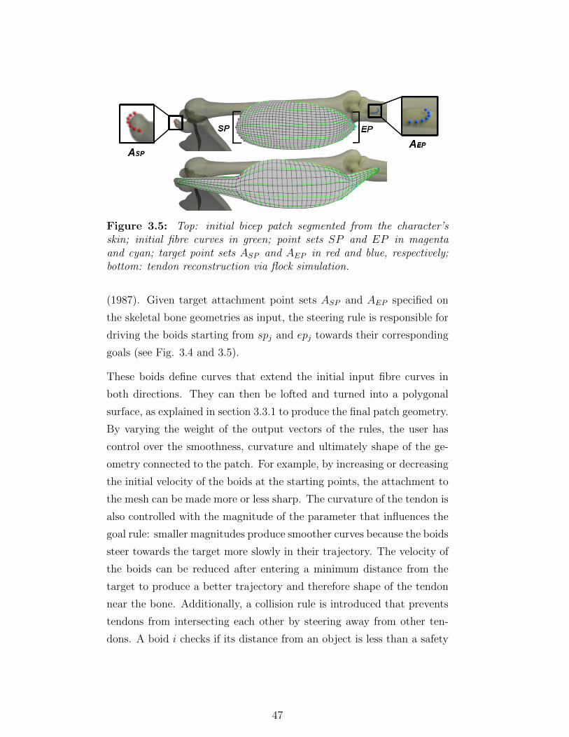
Figure 3.5: Top: initial bicep patch segmented from the character’sskin; initial fibre curves in green; point sets SP and EP in magentaand cyan; target point sets ASP and AEP in red and blue, respectively;bottom: tendon reconstruction via flock simulation.
(1987). Given target attachment point sets ASP and AEP specified on
the skeletal bone geometries as input, the steering rule is responsible for
driving the boids starting from spj and epj towards their corresponding
goals (see Fig. 3.4 and 3.5).
These boids define curves that extend the initial input fibre curves in
both directions. They can then be lofted and turned into a polygonal
surface, as explained in section 3.3.1 to produce the final patch geometry.
By varying the weight of the output vectors of the rules, the user has
control over the smoothness, curvature and ultimately shape of the ge-
ometry connected to the patch. For example, by increasing or decreasing
the initial velocity of the boids at the starting points, the attachment to
the mesh can be made more or less sharp. The curvature of the tendon is
also controlled with the magnitude of the parameter that influences the
goal rule: smaller magnitudes produce smoother curves because the boids
steer towards the target more slowly in their trajectory. The velocity of
the boids can be reduced after entering a minimum distance from the
target to produce a better trajectory and therefore shape of the tendon
near the bone. Additionally, a collision rule is introduced that prevents
tendons from intersecting each other by steering away from other ten-
dons. A boid i checks if its distance from an object is less than a safety
47

Figure 3.6: (a) Deltoid extruded patch; (b) inflated muscle; (c) newrest shape after smoothing and relaxation.
offset d and steers away from it using the vector:
steericoll = projTan(niclosest, (pbary − pi))− vi
where pbary is the barycenter of the rest of the flock, pi and vi are the
current position and velocity of boid i and projTan is a function that
returns the tangent component of an input vector given the normal at
the closest point on the mesh niclosest. The magnitude of steericoll is
clamped to a maximum allowed value.
3.3.3 Generation of muscles geometry
The initial patches are three-dimensional open manifolds. The next step
of the method is to find a way to turn these surfaces into closed meshes
obtaining plausible muscle shapes. The patches are, by construction,
very close to each other but not intersecting. Therefore the desired rest
closed configuration of the patch is forced to be very thin. The approach
one can take to create a closed volumetric mesh approximating the shape
of a muscle is to use a hole-filling algorithm with fairing (Liepa (2003)),
to triangulate the patch hole and then deflate it until it collides with
the patch itself. The problem with this approach is that the topology of
the filled part is not easily controllable and the triangulation does not
respect the desired edge flow.
Instead this method proceeds by extruding the initial patch by a very
small controllable offset. By extrusion it is meant that every vertex is
48

moved in the normal direction and the offset controls the distance by
which the vertex is moved. Then in a first phase pressure is applied to
the extruded vertices and a simulation without collisions is run until full
inflation. Using the resulting mesh, a new rest shape is generated by
applying alternated Laplacian smoothing iterations and tangential mesh
relaxations only on the inflated vertices (see Fig. 3.6). The iterations
continue until an initial estimate of the volume is reached. This step is
needed so that the resulting mesh is much less likely to create unwanted
folds when inflated. In a second phase, the actual simulation with colli-
sions is run in which final muscles are created. At the very start of the
simulation, the vertex positions of the initial extruded vertices constitute
the initial conditions applied to the rest shape created in the first phase,
so there is a non-negative elastic potential.
Inspired by the physics of rubber balloons (Skouras et al. 2012), increas-
ing pressure forces are applied to the nodes of the closed elastic patch,
towards the skeleton. During inflation, the vertices of the initial patch
with tendons are set fixed as Dirichlet boundary conditions and are not
allowed to move in order to obey the user input. In this process de-
formable meshes collide with other inflating patches and with the rigid
skeletal bones (see Fig. 3.7). The inflation continues until a desired vol-
ume amount is achieved or until a specified percentage of the total area
is in contact.
When inflating, artistic control is important to direct how the shape
evolves in time. For this reason artists have full control over the pressure
parameters of individual muscles. Even if not implemented, it would be
simple to integrate the support for painted spatial pressure weight maps
(per vertex) to give even greater control.
3.3.3.1 Elastic Model and Forces
The forces involved in the simulation are the stretching and pressure
forces. Inspired by the work of Wang et al. (2011), the rest pose of
the inflatable patches is represented in a two dimensional material space
computing for each triangle material coordinates of undeformed and de-
49
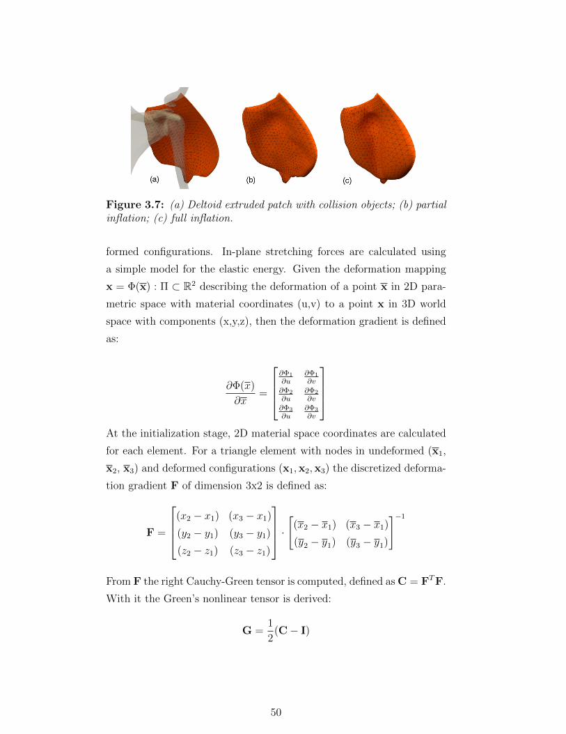
Figure 3.7: (a) Deltoid extruded patch with collision objects; (b) partialinflation; (c) full inflation.
formed configurations. In-plane stretching forces are calculated using
a simple model for the elastic energy. Given the deformation mapping
x = Φ(x) : Π ⊂ R2 describing the deformation of a point x in 2D para-
metric space with material coordinates (u,v) to a point x in 3D world
space with components (x,y,z), then the deformation gradient is defined
as:
∂Φ(x)
∂x=
∂Φ1
∂u∂Φ1
∂v∂Φ2
∂u∂Φ2
∂v∂Φ3
∂u∂Φ3
∂v
At the initialization stage, 2D material space coordinates are calculated
for each element. For a triangle element with nodes in undeformed (x1,
x2, x3) and deformed configurations (x1,x2,x3) the discretized deforma-
tion gradient F of dimension 3x2 is defined as:
F =
(x2 − x1) (x3 − x1)
(y2 − y1) (y3 − y1)
(z2 − z1) (z3 − z1)
·[
(x2 − x1) (x3 − x1)
(y2 − y1) (y3 − y1)
]−1
From F the right Cauchy-Green tensor is computed, defined as C = FTF.
With it the Green’s nonlinear tensor is derived:
G =1
2(C− I)
50

From Hooke’s law, the in-plane stress is calculated using a linear stress-
strain relationship:
σ = B · ε
where B is a precomputed 3x3 symmetric stiffness tensor that depends
on Young’s modulus E and Poisson’s ratio ν (Muller & Gross 2004) while
σ and ε are expressed in Voigt form.
Considering that the surface should not present transverse shearing re-
sistance, B can be simplified from the original 9 parameters to 5 as in
Wang et al. (2011).
B =
b11 b12 0
b12 b22 0
0 0 b33
=
E
1−ν2 ν E1−ν2 0
ν E1−ν2
E1−ν2 0
0 0 E1−ν2 (1−ν
2)
The elastic potential energy density per triangle can then be defined as:
Ee =
∫Ve
1
2(G : B : G)dv =
1
2(G : σ) · Aeh
where Ae is the area of the undeformed element, h its thickness and
Ve = hAe its volume. The total stretching energy of the deformable
patch is obtained by summing up the contributions of all the elements:
Estretch =
faces∑i
Eie
Finally, stretching forces and the Hessian (needed for implicit integra-
tion) are obtained by analytical derivation solving: −∇x(Estretch) and
−∇x(∇x(Estretch)), respectively.
As described in Skouras et al. (2012), muscles inflate thanks to a discrete
nodal pressure force defined as:
fi =∑j∈Ni
1
3· pi · Ajnj
where Ni are the neighbouring triangles of vertex i, Aj and nj the area
51
and normal of triangle j, and pi is the base pressure per vertex. In
practice, small triangles present in the tendon region result in small
pressure forces, which prevent the tendon from fully inflating. Therefore
a unit area Aj for all triangles is used. Adapting a topology-independent
method such as the one presented in Cong et al. (2015) would be also
beneficial. Pressure per-vertex is increased linearly over time. When a
node collides, its pressure value is frozen to its last value, in order to
improve the solver’s stability.
Note that bending forces can be disregarded in the simulation because
the progressive pressure increments that define the shape over time cause
stretching forces to be very large and the most influential. When inflat-
ing, artistic control is important to direct how the shape evolves in time.
For this reason artists have full control of the single muscles pressure and
material parameters (E and ν) parameters by painting a spatial weight
map to create variations in the inflating behaviour.
3.3.4 Fibre Field
Having a volumetric fibre field segmented by muscles is very important
for a subsequent physics based simulation of a tetrahedral mesh with an
anisotropic constitutive model capable of contraction. Alternatively the
muscle geometries themselves can be tetrahedralized and simulated with
fibre activations and intercollisions.
One of the advantages of generating the closed patch by extrusion is that
the creation of the fibre field of the inflated muscle is greatly simplified.
In the method of this work, first the fibre curves are duplicated and
translated by the same extrusion offset. Triangle barycentric coordinates
are calculated for each control node of the curve so that the inflation
deformation can be transferred to the curves. The result is a set of
deformed fibre curves that follow the muscle (see Fig. 3.3d). From these
curves a three dimensional vector field of fibre directions is generated.
It is then stored on a grid that can be interpolated trilinearly inside the
volume.
52
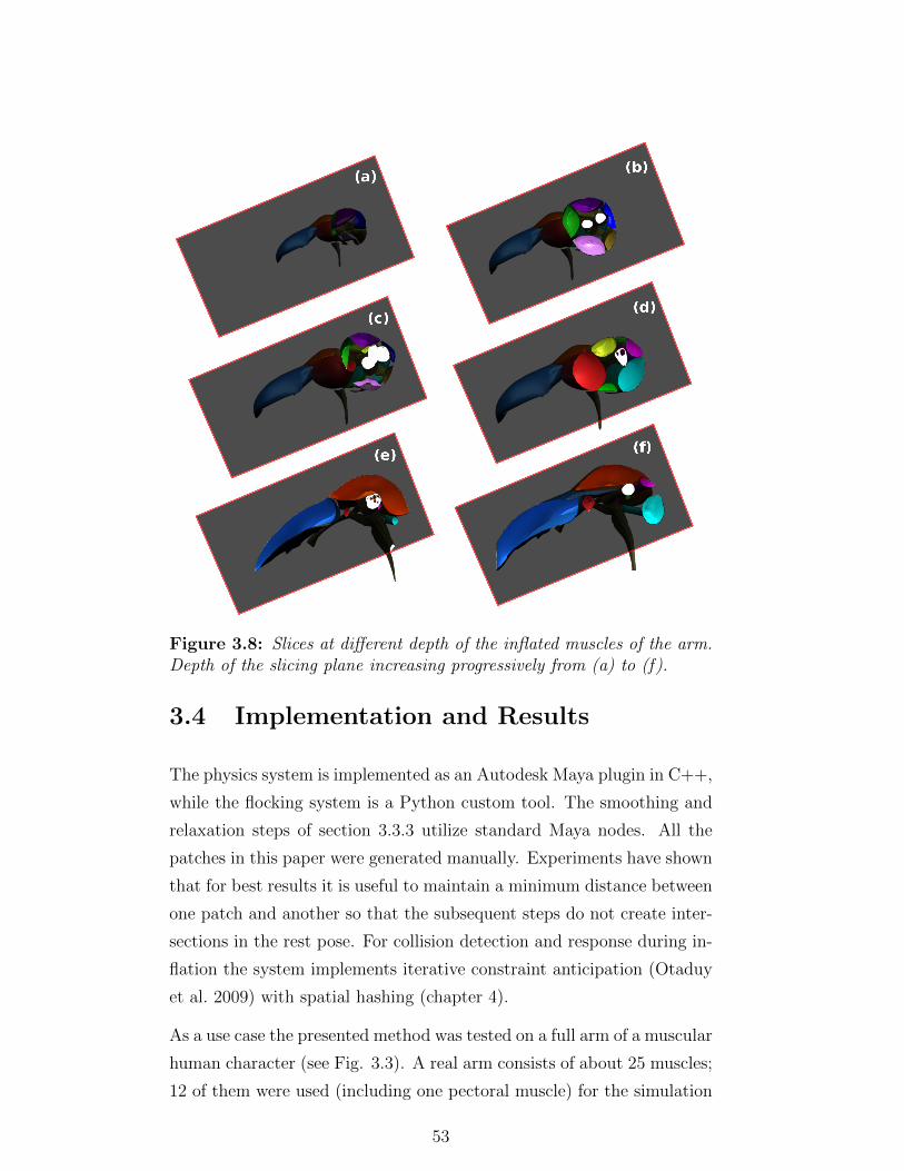
Figure 3.8: Slices at different depth of the inflated muscles of the arm.Depth of the slicing plane increasing progressively from (a) to (f).
3.4 Implementation and Results
The physics system is implemented as an Autodesk Maya plugin in C++,
while the flocking system is a Python custom tool. The smoothing and
relaxation steps of section 3.3.3 utilize standard Maya nodes. All the
patches in this paper were generated manually. Experiments have shown
that for best results it is useful to maintain a minimum distance between
one patch and another so that the subsequent steps do not create inter-
sections in the rest pose. For collision detection and response during in-
flation the system implements iterative constraint anticipation (Otaduy
et al. 2009) with spatial hashing (chapter 4).
As a use case the presented method was tested on a full arm of a muscular
human character (see Fig. 3.3). A real arm consists of about 25 muscles;
12 of them were used (including one pectoral muscle) for the simulation
53

as the rest are not superficial or do not contribute substantially to the
deformation. Thanks to the constraints represented by the still vertices
of the input patches, inflation produces reconstructions that the artist
can expect and control. To test performance, for simplicity the arm was
split in upper arm (8 muscles) and forearm (7 muscles) and simulated
separately (some shared muscles were duplicated for collision purposes).
In both cases inflating objects collide with each other and with the 6
rigid bones. Slices of the inflated resulting shapes are shown in Figure
3.8.
The test consists of a 400 frames long simulation computing 1 substep
per frame with a small timestep of 0.0005s and additive pressure in-
crease factor of 0.01 per frame. On an Intel Xeon X3470, the non-
optimized code runs on a single thread and takes a cumulative time of
904ms and 1222ms per substep for the 12K and 15K elements of fore-
arm and arm respectively. This result can be greatly improved with
multi-threading and, if desired, by trading the accuracy provided by a
constrained based collision system for a faster approach using penalty
forces (see Chapter 4). The validation has been done mainly at the qual-
itative and visual level, which was found satisfactory for the goals of the
project. A more rigorous approach would be to compare the arm mesh
simulated under the contraction of the fibres generated from sculpted
anatomical muscles from a template, with the mesh simulated thanks
to the active fibres obtained with the method in this Chapter. The
muscles and associated fibres produced with the method, despite not
being fully anatomically correct, present organic shapes that are usable
directly for the simulation of the character (for muscle contraction and
secondary effects) (see Fig. 3.9 and please refer also to the videos at
http://www.fabioturchet.com/supplemental_material.zip).
A method has been presented to generate volumetric muscles based on
input patches sketched on the surface geometry of a character. The
result is the ability to obtain simulation-ready muscle shapes along with
fibre fields to be used for further simulations. Having presented a way
54

Figure 3.9: (a) Generated bicep muscle; (b) Fibre curves and interpo-lated internal fibres; (c) Rest pose mesh; (d) Embedded mesh of deformedpose obtained using a tetrahedral FEM simulation with anisotropic ma-terial (isometric contraction).
to generate anatomical volumetric models, the next chapter describes
in detail the structure and theoretical foundations of the solver used to
simulate the tetrahedral meshes.
55

Chapter 4
Musculo-skeletal Simulation
4.1 Introduction
In Visual Effects one of the main requirements for computer-generated
creatures and humans is to look realistic, believable and fully integrated
in the context and world of the movie. One of the ways to convey this
realism is through realistic deformations of muscles, fat and skin.
In this chapter, the methods used to realistically deform anatomical mus-
cle shapes are discussed and, in particular, how fibre-activated materials
are integrated in the physics solver. In the first part of the chapter some
preliminary exploratory studies with existing technology conducted at
MPC will be presented followed by the custom framework that over-
comes the limitations encountered will follow.
4.2 Background
This work is based on the idea of applying an engineering approach
to character deformation. In an engineering context the Finite Element
Method is the most popular choice when simulating complex hyperelastic
behaviour of materials. Being in essence a method to find approximate
solutions to Partial Differential Equations, its theory has been very well
studied for decades.
56

After considering the various deformable models presented in Chapter 2
and with the desire to obtain plausible and stable results, a Lagrangian
representation with standard Finite Elements was chosen. This choice
was motivated by:
• The availability of a ready-to-use C++ open-source library for high
quality deformable objects called VEGA (Sin et al. (2013a)). Ex-
tending it and not coding it from scratch seemed a good idea
to speed up the implementation. Containing already classic hy-
perelastic materials (linear and corotational elasticity, StVk, neo-
Hookean, orthotropic), its interface made it quite easy to introduce
the anisotropic muscle material presented in section 4.3.3.
• The awareness that at the time of choice, existing interactive /
real-time methods were not mature enough, difficult to implement,
not accurate or not fully suitable for muscle simulation.
• A wide literature and documentation available on FEM for graph-
ics, including clear mathematical definitions of materials from en-
gineering research.
• The idea of using a top-down approach in the sense of first building
a system that is computationally complex but can achieve a desired
level of accuracy and progressively simplifying it to get a speed
trade-off. In this way it is made available a ground truth which
sets the baseline for comparison with later simplifications.
At MPC, FEM was very well known because of the existence of an in-
ternal destruction toolkit called Kali for the creation of effects such a
disintegration, fracturing and demolitions. Kali is an API built on top
of Pixelux’s Digital Molecular Matter (DMM) (Parker & O’Brien 2009)
and provides the artist with a set of tools and scripts to integrate DMM
into the FX pipeline to do mainly shots involving destructions, explo-
sions, fracturing and erosion.
However it soon became apparent, as detailed below, that Kali only
matches some of the requirements for muscle simulation and it was there-
fore discarded for the project. The limitation was not posed by FEM
57

itself, but rather by the lack of an adequate constitutive material model
to obtain volume-preserving active contractions of the deformable ob-
jects that represent muscles.
(a) (b)
Figure 4.1: (a) Slice of the full volumetric model; (b) Renderable skin
The tests described below were performed using existing technology at
MPC (i.e. Kali) to expose the necessity of research and development
on the flesh material and on the interaction of the different anatomical
layers. The goal of the following list of tests was in fact to prove that
what is achievable with the current simulation toolset at MPC is not
sufficient to achieve the desired quality of deformation. For simplicity
the focus has been put only on one part of the body, in particular the left
arm of a muscular male such as the one of a bodybuilder (Figure 4.1).
At the beginning of this process the muscle primitives of the existing
procedural system were fixed from all the intersections both with each
other and with the outer skin. Various amendments to the anatomy,
which in some cases was lacking accuracy at distal and proximal tendon
insertions, also had to be made. These changes were needed because
in the rest pose muscles should not have interpenetrations even if they
are in tight contact, otherwise the solver would start the simulation by
resolving those collisions, thus introducing spurious forces.
58
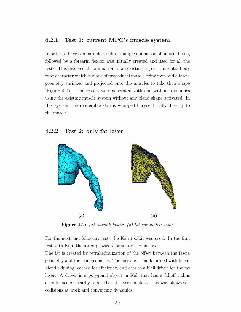
4.2.1 Test 1: current MPC’s muscle system
In order to have comparable results, a simple animation of an arm lifting
followed by a forearm flexion was initially created and used for all the
tests. This involved the animation of an existing rig of a muscular body
type character which is made of procedural muscle primitives and a fascia
geometry shrinked and projected onto the muscles to take their shape
(Figure 4.2a). The results were generated with and without dynamics
using the existing muscle system without any blend shape activated. In
this system, the renderable skin is wrapped barycentrically directly to
the muscles.
4.2.2 Test 2: only fat layer
(a) (b)
Figure 4.2: (a) Shrunk fascia; (b) fat volumetric layer
For the next and following tests the Kali toolkit was used. In the first
test with Kali, the attempt was to simulate the fat layer.
The fat is created by tetrahedralization of the offset between the fascia
geometry and the skin geometry. The fascia is then deformed with linear
blend skinning, cached for efficiency, and acts as a Kali driver for the fat
layer. A driver is a polygonal object in Kali that has a falloff radius
of influence on nearby tets. The fat layer simulated this way shows self
collisions at work and convincing dynamics.
59

4.2.3 Test 3: simulated passive muscles
(a) (b)
(c)
Figure 4.3: (a) Skeleton ; (b) Attached muscles; (c) Muscle deformation
In this test each muscle primitive was first tetrahedralized, detaching
their connections from the procedural system to keep only the geometry.
Then these muscles were constrained at their extremities through drivers
(the attachment points corresponding to the tendons) and fed into the
solver. The result is a set of deformable wobbly objects colliding with
each other but not really expressing the characteristics of muscles (Figure
4.3). The simulation was then transferred directly to the outer skin layer
with a wrap deformer.
60
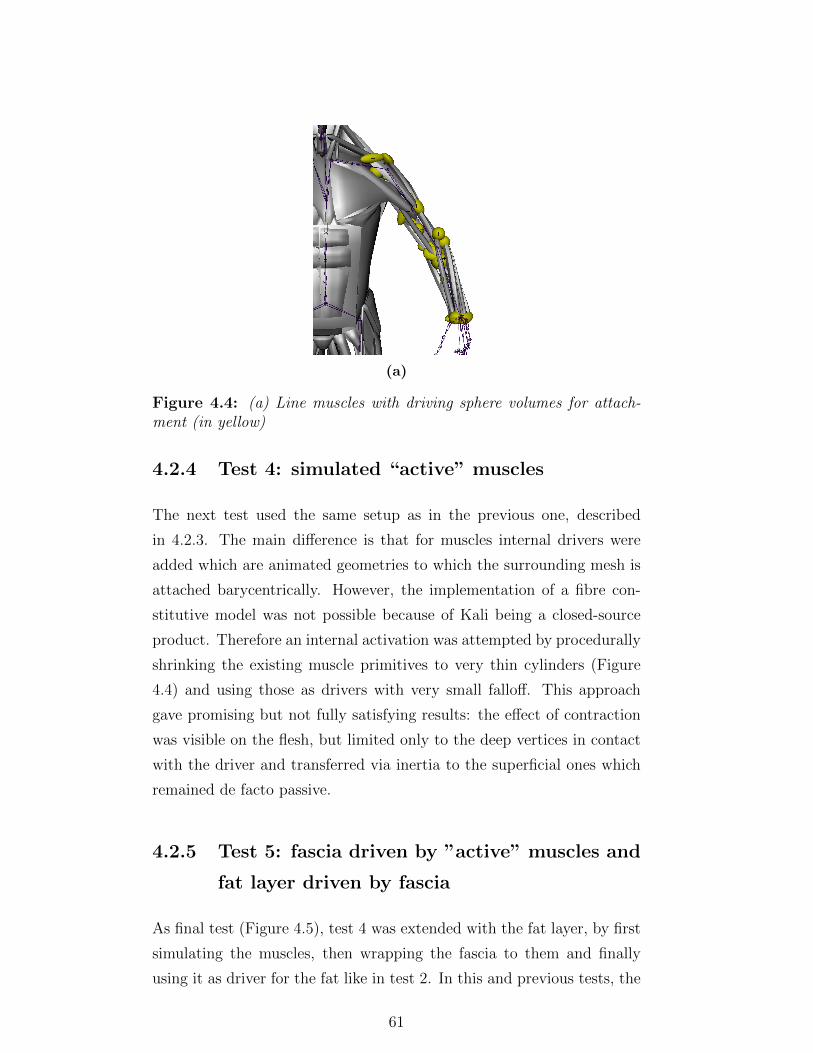
(a)
Figure 4.4: (a) Line muscles with driving sphere volumes for attach-ment (in yellow)
4.2.4 Test 4: simulated “active” muscles
The next test used the same setup as in the previous one, described
in 4.2.3. The main difference is that for muscles internal drivers were
added which are animated geometries to which the surrounding mesh is
attached barycentrically. However, the implementation of a fibre con-
stitutive model was not possible because of Kali being a closed-source
product. Therefore an internal activation was attempted by procedurally
shrinking the existing muscle primitives to very thin cylinders (Figure
4.4) and using those as drivers with very small falloff. This approach
gave promising but not fully satisfying results: the effect of contraction
was visible on the flesh, but limited only to the deep vertices in contact
with the driver and transferred via inertia to the superficial ones which
remained de facto passive.
4.2.5 Test 5: fascia driven by ”active” muscles and
fat layer driven by fascia
As final test (Figure 4.5), test 4 was extended with the fat layer, by first
simulating the muscles, then wrapping the fascia to them and finally
using it as driver for the fat like in test 2. In this and previous tests, the
61

(a) (b)
(c) (d)
Figure 4.5: Deformation of (a) Muscles; (b) Fascia; (c) Fat; (d) Ren-derable skin
bones are tetrahedralized as well and treated as rigid bodies. This setup
produced the most realistic results.
4.2.6 Analysis of the tests
What emerged from all these experiments was in part expected. First
of all it is clear that muscles cannot be simulated with just position
constraints and an isotropic material. They need a fibre-embedded di-
rectional material model to behave realistically. In addition to this basic
requirement, the results obtained are convincing in terms of dynamics
and shape: separating the jiggle of the muscles from the jiggle of the fat
seems to give more realism and also the self collisions seem to add a lot
to the flesh look of the arm. The ulna colliding with the skin gives a nice
shape to the elbow (Figure 4.5d).
62
It became apparent that not only is a good anatomical model with prop-
erly placed constraints essential, but also that biomechanical require-
ments should be formalized and implemented carefully. For example,
the radius/ulna rotation should be treated carefully to avoid problems
during pronation and supination such as artifacts on the final renderable
skin. Problems due to the initial rest shape also appeared in the exam-
ple with the brachialis muscle in which the model was provided as two
disjoined mesh objects. As a consequence, during forearm flexion and
extension its geometry created a depression on the skin.
One of the limitations of these tests is that a different stiffer material
was not assigned to the part of the geometry belonging to tendons. The
examples clearly demonstrate the need for a more advanced system that
supports features such as: sliding of the components under the fascia
and the skin, activations, multiple constraints types, fascia simulation.
Tests also show the fact that it is necessary to create the connective
tissue constraints between muscles to keep them together during ballistic
motion. Muscles in fact should behave as a whole during high-inertia
animations such as jumps.
4.3 Solver and Material Models
The approach taken aims at achieving high levels of realism by simulating
ordered layers of biological tissues, from the inside to the outside, so that
the interesting looking nonlinearities that result from their interaction
can be captured. This means that the simulation will be split in different
stages, each one outputting an intermediate product of the final result
(layers). This makes the system modular and more controllable, but at
the same time makes the coupling of the forces more difficult to achieve.
4.3.1 Simulation Model Construction
In order to test the hypothesis that anatomy-based character simulation
is a potentially beneficial technique to be adopted by the company, a
63

working prototype is needed. The aim of the prototype is also to find
the weaknesses and the possible points of improvement from a practi-
cal point of view. This process begins by choosing the musculo-skeletal
model to be simulated. Even though there are commercially available
solutions such as Zygote (Zygote 2016), for the use case scenario of in-
terest the choice goes to the model of an arm (CGCircuit 2016) obtained
by retopologizing scans from a database of real muscles complete with
tendons (see Fig. 4.6). The models therefore are very accurate and the
mesh clean. Skeleton geometry is obtained in the same way. The model
consists of 4 bones and 14 muscles. It is important to have a mesh
with regular polygons to facilitate the subsequent generation of regular
tetrahedra out of them and improve the collision response accuracy. As
shown in the previous section, the option of converting the procedural
muscle primitives used in the rigging department was excluded because
the shape was is not anatomically accurate enough. For simplicity some
of the muscles were merged in bigger groups easier to handle, but still
keeping the superficial details. In particular this was done for some of the
many thin adjacent muscles of the forearm such as extensors and flexors
which are approximated to be working together (see section 4.4.2). Fewer
muscles also mean fewer computations for a collision system and fewer
constraints between them. Therefore the decision taken is to trade-off
the accuracy of interaction of muscles for speedup. These triangle meshes
are then converted into a volumetric tetrahedral representation using in-
ternal tools available from the Kali toolset which allow the control of
various aspects of the tetrahedralization: number of elements, confor-
mity, custom density via weight maps.
4.3.2 Solver
The solver is the core part of any simulation system. On it directly
depend desirable qualities such as speed, accuracy of the output, stability
of the simulation. In the context of this thesis it has to integrate a
partial differential equation (PDE) expression of Newton’s second law,
commonly known in continuum mechanics as the Cauchy momentum
64

Figure 4.6: Anatomical geometry for prototype testing. On the left therenderable/embedded mesh from which its conforming volumetric coun-terpart is generated (right).
equation which relates the acceleration of a point in a medium with the
forces it receives from the surrounding material:
ρdv(X)
dt= ∇ · σ + ρb
where ρ represents the density of the material, v(X) the velocity of a
material particle in the object, σ the Cauchy stress distribution (force
associated with the deformation of the object) and b the body forces
(gravity, collision response etc).
When testing a solver, it is common in the literature (McAdams et al.
2011) to first study the physics of deformable objects in a quasistatic
setting, meaning finding the configuration that brings in equilibrium the
forces of the system excluding gravity and inertial effects. By equilibrium
it is implied that the sum of all the forces equals zero. This is the
65

approach also followed in this work for the deformation of muscles, while
dynamics are introduced in a second stage.
In this work objects (meshes) are intended to be defined as a connected
collection of nodes and elements. The nodes are the points for which
positions and velocities need to be calculated given the current inertial
motion of the object, its material and the presence of external forces. In
the Finite Element Method and elasticity theory, objects are first dis-
cretized into surface (triangles) or volumetric (tetrahedra) elements on
which physical properties such as forces are defined and calculated. In
a second stage the method takes the contributions of each element and
assembles them in a global system matrix that expresses the accumula-
tion of the elastic forces on each node, shared by multiple elements. A
deformation can be formalized at each material point of an object as a
function that maps a point in material space x ∈ R3 to a point in world
space X ∈ R3:
Φ : Ω→ R3
x = Φ(X)
As mentioned before, a deformation metric has to be chosen. The ba-
sic deformation quantifier is the deformation gradient F, a 3x3 matrix
defined as the Jacobian of the deformation function:
Fij = ∂Φi/∂Xj (4.1)
In practice other metrics dependent on F are used such as Green’s strain
E (used in this work) which, despite being more computational expen-
sive, is independent of the rotation of the element:
E =1
2(FTF− I) (4.2)
Knowing the severity of deformation is just one of the ingredients needed
to define the physics of deformable objects.
66
Using E it is in fact possible to define a material model that expresses
the relationship between stress and strain and captures the elastic energy
accumulated in a deformed state at a certain time. At a mathematical
level a material is an energy density function Ψ that represents the elastic
energy of an element. The total elastic energy in a continuous setting is
just the integral over the elements of this density function:
Wtot =
∫ω
Ψ(X,F(X))dX
A real world example of such a function is the one for St. Venant-Kirchoff
materials:
Ψ(F) = µE : E + λtr2(E) (4.3)
where µ and λ are the Lame’ coefficients which are related to standard
material properties used in continuum mechanics such as Young’s Mod-
ulus Y (measure of stretch resistance) and Poisson ratio ν (measure of
incompressibility):
µ =Y
2(1 + ν)
λ =Y ν
(1 + ν)(1− 2ν)
The strain tensor is a quantity that measures the amount of normalized
displacement with respect to a rest configuration. It can also be seen
as expressing how much the deformation gradient F differs from the
identity:
ε =∂(x−X)
∂X= F− I
The (Cauchy) stress tensor instead is a quantity that expresses how much
force f acts on a cross sectional surface area of a solid and depends on
the direction of the surface:
σ · n = f
It can also be thought as the sum of two components: a mean (or dila-
67
tional) tensor (responsible for volume changes) and a deviatoric tensor
which is actually responsible for distortion and deformation.
In material science literature the properties of a material subject to in-
creasing loading are often visualized through a strain/stress plot that
describes the relation of deformation to accumulated stress for a mate-
rial constitutive model.
After applying FEM theory to the equation of motion (Eq. 2.1), ex-
pressing it in terms of positions (displacements) and adding a velocity
damping term it becomes:
Mq + Dq + fint(q) = fext
where q ∈ R3m are the displacements of the m mesh vertices from the
rest configuration, D = αM + βK(q) + D is the damping matrix, fint
represents the internal elastic forces (gradient of the elastic energy) and
its gradient with respect to u, K, is the tangent stiffness matrix.
In order to timestep this equation, in VEGA the Implicit Backward Euler
integration scheme is adopted, in its semi-implicit form (Baraff & Witkin
1998):
qn+1 = qn + hvn+1
vn+1 = vn + hM−1(fext − fint(qn+1)−Dvn+1)(4.4)
By linearizing the nonlinear fint via Taylor expansion:
fint(qn+1) = fint(qn) + K(qn+1 − qn)
The equation becomes linear:
(M + hD = h2K)(vn+1 − vn) = h(fext − fint(qn)−Dvn − hKvn)
By knowing the stress that an element undergoes, it is possible to com-
68
pute the internal forces acting on it. In VEGA this is done by using the
first Piola-Kirchoff stress tensor P defined as:
P(F) = ∂Ψ(F)/∂F
Once P(F) is computed, the force on a vertex of a tetrahedron is obtained
by multiplying P(F) with its area-weighted normal:
G = PBm (4.5)
where G is the matrix having the forces acting on each vertex of a tetra-
hedron and Bm is the matrix having as vectors the area-weighted normals
(Irving et al. 2004).
Therefore, in order for the method to work, for each element the stiffness
matrix K has to be computed. K is defined as the gradient of the internal
forces, but in practice its implementation makes use of P (Sin et al. 2011):
K =∂G
∂q=∂G
∂F
∂F
∂q= (
∂P
∂FBm)
∂F
∂q
Details on the derivations can be found in Sifakis & Barbic (2012).
In production, it is highly desirable to give technical artists a fast initial
approximation of the results they will get so that they can do more
iterations of creative work. To this purpose the solver should support
mechanisms to trade-off speed for accuracy and be consistent in relation
to sub-frames and resolution variation.
One of the standard techniques adopted in this work to achieve this and
to reduce the computation time is called mesh embedding, in which the
momentum equation is not solved on all the nodes of a high-resolution
mesh, but on a coarse version of the same. The final, renderable mesh is
then deformed from this low-res version using barycentric coordinates.
Moreover, it is possible to reduce the number of elements (tetrahedra)
of the volume by allowing one tetrahedron to share different materials.
This approach, not implemented in this work, is used in (Saito et al.
2015) where the quantities of each material are calculated with Monte-
69

Carlo integration. Another practical solution would be to integrate into
the rig blend shapes obtained with simulation.
4.3.3 Constitutive Material Model
Given their structure and specific properties typical of most biological
tissue, muscles have been described by an incompressible, transversely
isotropic, hyperelastic material. Transversely isotropic means that its
physical properties are symmetric with respect to an axis which is per-
pendicular to an isotropy plane (see Figure 4.7): the properties are the
same on the same plane in all directions.
Figure 4.7: Transverse isotropy
One of the materials for muscles found in the literature (Teran et al. 2003)
and implemented in this work has an uncoupled energy form, separating
the material response due to isotropic passive connective tissue and to
active components:
W(I1, I2, λ, a0, α) = F1(I1, I2) + U(J) + F2(λ, α) (4.6)
where:
• C = J−23 FTF is the right Cauchy-Green deformation tensor
70

• I1 = tr(C) is the deviatoric (non-volumetric) invariant of the strain
• I2 = 12((tr(C))2 − tr((C2))) is the isotropic invariant of the strain
(does not vary in magnitude when measured in different directions).
An invariant is the same for different orientations of the coordinate
system chosen)
• λ =√
a0 ·Ca0: a strain invariant associated with transverse isotropy.
Transverse isotropy indicates that physical properties are approx-
imately the same along a plane (it equals the deviatoric stretch
along the fibre direction)
• a0 is the fibre direction vector that doesn’t depend on F
• α represents the level of activation in the tissue
• F1 is a Mooney-Rivlin rubber-like model that encapsulates the
behaviour of the isotropic tissues in muscle that embed the fascicles
and fibres. In this work the StVk model is used instead
• J = det(F) is the measure of relative volumetric deformation of
the element.
• U(J) is a term expressing incompressibility
• F2 is the active and passive muscle fibre response. It depends on a0,
the deviatoric stretch in the along-fibre direction λ, the nonlinear
stress-stretch relationship in muscle and α.
This material is popular in muscle simulation literature and is intended to
capture the force-length nonlinear relationship obtained experimentally
from the study of individual fibre response (Teran et al. 2003) (Figure
4.8)
In this work, it is assumed that the stress P and the stiffness matrix K
are composed of isotropic and anisotropic summable parts:
P = Piso + Paniso
K = Kiso + Kaniso
71
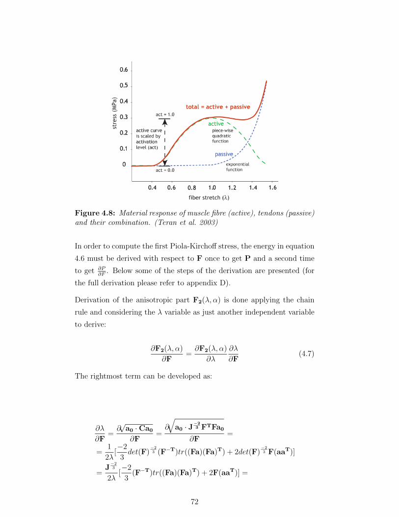
Figure 4.8: Material response of muscle fibre (active), tendons (passive)and their combination. (Teran et al. 2003)
In order to compute the first Piola-Kirchoff stress, the energy in equation
4.6 must be derived with respect to F once to get P and a second time
to get ∂P∂F
. Below some of the steps of the derivation are presented (for
the full derivation please refer to appendix D).
Derivation of the anisotropic part F2(λ, α) is done applying the chain
rule and considering the λ variable as just another independent variable
to derive:
∂F2(λ, α)
∂F=∂F2(λ, α)
∂λ
∂λ
∂F(4.7)
The rightmost term can be developed as:
∂λ
∂F=∂√
a0 ·Ca0
∂F=∂
√a0 · J
−23 FTFa0
∂F=
=1
2λ[−2
3det(F)
−23 (F−T)tr((Fa)(Fa)T) + 2det(F)
−23 F(aaT)]
=J−23
2λ[−2
3(F−T)tr((Fa)(Fa)T) + 2F(aaT)] =
72
=J−23
λ[−1
3(F−T)tr((Fa)(Fa)T) + F(aaT)] (4.8)
The anisotropic term F2 is defined in Blemker et al. (2005) as
F2(λ, α) = αFactive(λ) + Fpassive(λ)
where Factive and Fpassive are defined as a piecewise combination of
simple linear and exponential functions, therefore it’s enough to take
their analytical derivatives.
In order to support invertible elements recovery (Irving et al. 2004),
the diagonalized version of F is F = UFVT which allows carrying out
substitutions in the formula:
F⇒ F
FT = F
a0 = VTa0
The last line is needed to rotate the anisotropic terms using V, as sug-
gested in Irving et al. (2004), so that the final formula becomes:
Paniso =∂F2(λ, α)
∂F=∂F2(λ, α)
∂λ
(1
2λVTa0 · 2(−1
3J2F + J−
23 FOnes)VTa0
)(4.9)
with
λ =
√VTa0 · J
−23 F2VTa0
J = det(F)
In order to compute the anisotropic part of the stiffness matrix, P has to
be derived a second time yielding the formula (using Einstein’s notation):
73

∂Paniso
∂F=− 2
9J−23 (F−T)ij(a0 · J
−23 FTFa0)
−12lm (F−T)ij(Fa)k(Fa)k
− 2
3J−23 (F−T)ij(a0 · J
−23 FTFa0)
−12lm (Fa)iaj
(4.10)
The incompressibility term of the energy is defined in Teran et al. (2003)
as:
U(J) = K ln(J)2
and its derivative becomes:
∂U(J)
∂F=∂U(J)
∂J
∂J
∂F=
2K ln(J)
Jdet(F)F−T = 2K ln(det(F))F−1
However, in this work the incompressibility term U(J) is already incor-
porated in term F1 which is in fact represented by an isotropic StVK
material. Expressions for ∂Piso/∂F are implemented in VEGA, but not
in their analytical efficient form. Therefore the formulation was derived
by hand (shown below). Full derivation is given in appendix C.
Piso = P(F) = F[2µE + λtr(E)I] (4.11)
∂Piso(F)
∂F=∂(F[2µE + λtr(E)I])
∂F=
= µ(δipFTF)qj + (FTF)piδjq + FT
qiFpj − δipδjq)+
+1
2λ(2FpqFij + δipδjqtr(F
TF)− 3δipδjq)
(4.12)
which is a 4th order tensor with indices (i, j, p, q).
Once Piso and Paniso are computed, using equation 4.5 the forces can be
calculated and also the final combined stiffness matrix, sum of Kiso and
Kaniso, for Implicit Euler integration.
74

4.3.4 Boundary Conditions (Constraints)
In practical applications a deformable body does not serve any particular
purpose if it is just free moving. Most of the interesting behaviour of
physical objects derives from their interaction with other objects, user
manipulation and fixed or moving constraints of some of their parts.
Formally this translates into adding initial and boundary conditions and
constraints to be taken into account when solving the PDE of motion.
For instance vertices of the mesh could be required to keep a fixed posi-
tion in space or to follow a position at an offset relative to another object
(like muscles relative to bones), or they could be required to slide over
another object, or again to not compenetrate other meshes. In addition
to the uses described above, constraints are really important in the con-
text of this work because they allow the composition and interconnection
of anatomical layers, coupling them between each other to transfer across
inertia.
In terms of collision/self-collision resolution and response, typical cases
arise when muscles of different groups or fat get in contact: during an
arm flexion for example the lateral bulging is due to the pushing of soft
tissues against each other and to the physiological muscle bulging due
to contraction. Moreover, when two or more characters are interacting
(during a fight for example), the effect of collision forces is very evident
and the result on the skin contributes the level of drama in the action,
especially in slow-motion shots where contacts cause wave propagation
of the stress on the tissues. More details about the implementation and
the data structures used for the collision system are given in chapter 3.
The framework developed for musculo-skeletal simulation is based on
VEGA with custom implementations of constraints and collision re-
sponse. The first version of this framework models constraints and col-
lisions using elastic spring potentials. At a later stage this version was
successively improved using a constraint-based dynamics approach (the
framework which was used in Chapter 3). The results on muscle simu-
lation presented in this chapter were obtained using the first version of
the framework. Below details on the two methods are given.
75

4.3.4.1 Springs view
Spring constraints consist of two mass points connected by a virtual
spring characterized by parameters such as rest length and stiffness con-
stant (Nealen et al. 2006). When the vector q connecting start and end
of the spring is different in magnitude than the rest length r, an elastic
response force dependent on the elastic coefficient ks is generated.
W(q) = ks|||q| − r||2 (4.13)
Position and sliding constraints can be hard or soft. Hard con-
straints can be thought as infinitely stiff springs, keeping the end points
always at the same initial distance. Soft constraints instead are springs
with a stiffness constant low enough to produce “bouncy” behaviour. At
each frame the new positions of the end points are read from the mesh
data structure, and their distance is used to compute the Jacobian of the
energy:
f(q) = ks(|q| − r)q
|q|(4.14)
Indicating with I the identity matrix, the Hessian of the spring potential
(Choi & Ko 2002) becomes:
∂f
∂q= ks
[(1− r
|q|
)I +
r
(|q|)qqT
](4.15)
The constraints force contributions are accumulated in the external forces
vector and the Hessians are added to the global stiffness matrix. Slid-
ing constraints differ from the position ones for the fact that the x, y, z
coordinates of one of the end points is determined using a closest point
query from one object to the other.
The offending vertices on which collision forces are computed are the
ones of the high resolution embedded mesh, but the solver deals internally
with simulation of the tetrahedral mesh only. Therefore using barycentric
coordinates the forces are distributed to the tetrahedral nodes.
Collision/self-collision constraints implemented as springs are based
76
on the penalty method. After a collision is detected, to prevent mesh
compenetrations in the next timestep a response has to be generated in
the form of repulsion force. The penalty method tries to prevent a vertex
of a mesh entering another mesh by checking if the point lies within a
threshold distance from the object and if so, instantiating a zero-length
spring that applies a penalty force proportional to the penetration depth
d. This method is not fully free of self-penetrations. In order to have
more responsive collisions, in this work the penalty force is an exponential
function of d.
4.3.4.2 Constrained Dynamics view
The other way to treat collision responses is by incorporating mathemat-
ically defined constraints of the form C(x) = 0 into the dynamics system
matrix and solve the resulting Linear Complementarity Problem (LCP).
With this system it is in theory impossible that the constraints are vio-
lated and the output is velocities of the deformable object’s vertices that
are guaranteed to not intersect.
For position and sliding constraints the mathematical form is:
C(pA, pB) = nT (pA − pB) ≥ 0
where the normal for the position type is:
n =pA − pB|pA − pB|
for the sliding type is n = nobjectB and for the collision/self-collision
type n is the collision normal.
A constrained dynamics system was implemented at MPC after the work
produced in this Chapter by an intern student (Haapaoja 2016) and
successively improved by me and used in Chapter 3. Please refer to
Haapaoja (2016) for in-depth details on the collision system used. More
details on constrained dynamics can be found in Otaduy et al. (2009)
and Tournier et al. (2015).
77

4.4 Implementation and Results
In this section the details of the setup and simulation of the prototype
anatomical arm example are presented, in particular the layered ap-
proach inspired by previous work (Lee et al. (2009), Comer et al. (2015)
and Clutterbuck & Jacobs (2010)).
The formulation presented in the previous sections was ported to code
following the interfaces provided by the library VEGA and extending
classes IsotropicMaterial, isotropicHyperelasticFEM, isotropicHyperelas-
ticFEMForceModel. In particular, the simulation loop algorithm can be
summarized as follows:
1: for each element do2: Compute F from its vertex positions (eq. 4.1);3: Compute dP/dF (eq. 4.12 and eq. 4.10);4: Compute Kiso and Kaniso (eq. 4.3.2);5: Accumulate result to global stiffness matrix;6: end for7: for each spring constraint (if any) do8: Compute its K and accumulate to global stiffness matrix;9: end for10: Prepare multibody system matrix A using Implicit Euler;11: Solve for velocities ∆v;12: for each constraint expressed as C(x) = 0 (if any) do13: Add its contribution to Jacobian matrix;14: end for15: Solve LCP and add ∆v to unconstrained velocities;16: Use new velocities to compute new positions;
Algorithm 1: Pseudo code for the simulation loop
In terms of contact detection, the method in McAdams et al. (2011)
could also be implemented. In it the high-resolution mesh is sampled
(proxy points xp). For each sample, first its barycentric coordinates
with respect to the closest deformed tetrahedra containing it are calcu-
lated. The iso-value of the material point obtained is then calculated
for a level set in the undeformed configuration and the closest point on
the undeformed surface selected. This point xs is then queried back in
the deformed configuration so that the penetration depth and normal
78
are |xs − xp| and (xs−xp)
|xs−xp| respectively. When a collision is detected, zero
length anisotropic springs are created between xs and xp so that there
is a sliding effect on the plane perpendicular to the penetration direction.
4.4.1 Bones
Bones are treated as articulated rigid bodies, inheriting exactly the same
transformation as the corresponding Maya bone in the driving rig. The
shape of bones at their extremities is generally irregular and the cor-
responding joints are simplified using models common in robotics. For
example the elbow is represented with hinge joints, assuming the rotation
happens on one constant axis; the humerus is a ball-socket joint. The
underlying rig implements rotation of the radius over the ulna during
pronation and supination of the forearm. In the examples of this section
the skeletal bones used are: scapula, humerus, radius, ulna of the right
arm/forearm.
4.4.2 Muscles and Tendons
The 3D muscles in the prototype are represented as a set of volumetric
elements with embedded fibre directions that follow the transformation
of the bones they are attached to. The 14 muscles simulated in the
examples below are:
• Biceps Brachii, Lateral Triceps Brachii, Medial-long Triceps Brachii,
Brachialis, Anconeus
• Superficial extensors (combo of brachioradialis, Extensor Carpi Ra-
dialis Longus, Extensor Carpi Radialis Brevis), Extensor Digito-
rum, Extensor Digitorum, Pronator Teres, Flexor Carpi Ulnaris,
• Flexors (combo of Flexor Carpi Radialis, Palmaris Longus, Flexor
Carpi Ulnaris), Extensor Carpi Ulnaris, Flexor Digitorum Superfi-
cialis, Flexor Carpi Ulnaris, Abductor Pollicis Longus.
79
In this setup, muscles are attached to the bones geometry typically at
two points, proximal (origin) and distal (insertion) following anatomical
references found in medical literature and online (Zygote Body 2016).
To this aim, vertices of the tetrahedral mesh are pinned to the bone
mesh via position (hard) constraints. Some muscles like the deltoid, bi-
ceps brachii, triceps or the gastrocnemius (calf) have two or three heads
with which they attach to two or more bones they span: these muscles
are a unique mesh but often they are modelled as separate geometries
because splitting them enhances modularity and finer control of defor-
mation over specific parts. On the other hand, given the vast number of
superficial muscles on the forearm, it is also beneficial for the purpose
of faster simulation times to group adjacent muscles together. These
simplifications are generally decided beforehand and in general they do
not affect the visual result: muscles are tightly packed together and for
many movements they move in sync.
Once the models are created, tetrahedralized and attached to the bones
using anatomically-based constraints, the next step is to continue the pre-
processing by defining the per-element fibre directions. The anisotropic
material defined in section 4.3.3 has to express the state of the fibres that
can be active or passive. The peculiar characteristic of the muscle tissue
is its ability to contract and assume different shapes as a consequence.
The visual appearance of muscles bulging is determined at the micro
level by the activation of a huge number of fibres that slide over each
other due to biochemical firing processes. Muscles bulge in fact because
these fibres overlap one on each other during contraction, shortening the
muscle belly and stretching the tendons. Moreover, blood permeates the
tissues therefore, being a fluid, volume has to conserve.
In practice these requirements translate into an extension of the passive
volumetric model with an embedded 3D fibre field that can be thought
of as a flow from tendon origin(s) to tendon end(s) and which makes the
material stiffer in their direction when activated (anisotropy). Initially
the fibres were intended to be modelled semi-automatically as explained
in (Saito et al. 2015): solving a Laplace flow equation from the origin to
the insertion positions on the tendon with mixed boundary conditions
80
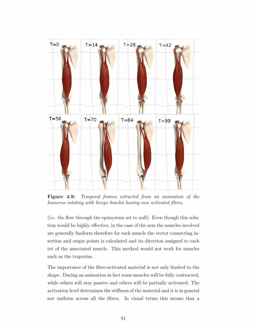
Figure 4.9: Temporal frames extracted from an animation of thehumerus rotating with biceps brachii having non activated fibres.
(i.e. the flow through the epimysium set to null). Even though this solu-
tion would be highly effective, in the case of the arm the muscles involved
are generally fusiform therefore for each muscle the vector connecting in-
sertion and origin points is calculated and its direction assigned to each
tet of the associated muscle. This method would not work for muscles
such as the trapezius.
The importance of the fibre-activated material is not only limited to the
shape. During an animation in fact some muscles will be fully contracted,
while others will stay passive and others will be partially activated. The
activation level determines the stiffness of the material and it is in general
not uniform across all the fibres. In visual terms this means that a
81

Figure 4.10: Temporal frames extracted from an animation of thehumerus rotating with biceps brachii having activated fibres.
contracted muscle appears to jiggle much less than a relaxed one. In the
example of a male athlete running, his pectorals appear very dynamic
because of the momentum of the soft tissue due to gravity and also due to
the balancing forces applied back in response to stepping on the ground;
but if he keeps them voluntarily contracted they appear much stiffer
and the noticeable jiggle is due mainly to the superficial adipose tissue.
Figures 4.9 and 4.10 illustrate this behaviour: the same animation of a
muscle constrained to rotating bones looks different if the fibres are not
firing (passive material) or are activated (material becomes stiffer and so
is less governed by inertial motion).
Muscle activations are a fundamental parameter of the anisotropic mate-
82
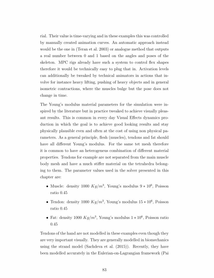
rial. Their value is time-varying and in these examples this was controlled
by manually created animation curves. An automatic approach instead
would be the one in (Teran et al. 2003) or analogue method that outputs
a real number between 0 and 1 based on the angles and poses of the
skeleton. MPC rigs already have such a system to control flex shapes
therefore it would be technically easy to plug that in. Activation levels
can additionally be tweaked by technical animators in actions that in-
volve for instance heavy lifting, pushing of heavy objects and in general
isometric contractions, where the muscles bulge but the pose does not
change in time.
The Young’s modulus material parameters for the simulation were in-
spired by the literature but in practice tweaked to achieve visually pleas-
ant results. This is common in every day Visual Effects dynamics pro-
duction in which the goal is to achieve good looking results and stay
physically plausible even and often at the cost of using non physical pa-
rameters. As a general principle, flesh (muscles), tendons and fat should
have all different Young’s modulus. For the same tet mesh therefore
it is common to have an heterogeneus combination of different material
properties. Tendons for example are not separated from the main muscle
body mesh and have a much stiffer material on the tetrahedra belong-
ing to them. The parameter values used in the solver presented in this
chapter are:
• Muscle: density 1000 Kg/m3, Young’s modulus 9 ∗ 106, Poisson
ratio 0.45
• Tendon: density 1000 Kg/m3, Young’s modulus 15 ∗ 106, Poisson
ratio 0.45
• Fat: density 1000 Kg/m3, Young’s modulus 1 ∗ 106, Poisson ratio
0.45
Tendons of the hand are not modelled in these examples even though they
are very important visually. They are generally modelled in biomechanics
using the strand model (Sachdeva et al. (2015)). Recently, they have
been modelled accurately in the Eulerian-on-Lagrangian framework (Pai
83

et al. 2014), even though their effect on the skin due to collision and
sliding was not modelled.
In Teran et al. (2005a) the connections between different muscles are
expressed through links (line segments). In the rest pose some points of
a source geometry are sampled (~xsamp) and for each one its closest point
~xanch (anchor) on all the neighbouring muscle surfaces is associated. Dur-
ing simulation the link with the closest anchor point becomes active and
determines the collision response force (with springs for example). At
each time step, the positions and the normal velocity components of a
sample are set to match the ones of its anchor:
~x′
samp = ~xsamp + α[(~xanch − ~xsamp) · ~N ] ~N
~v′
samp = ~vsamp + β[(~vanch − ~vsamp) · ~N ] ~N
where ~N indicates the normal at the surface point and α, β are control
coefficients. After having tried a similar approach for sliding, i.e. setting
explicitly the normal velocity of the sliding nodes (Warburton 2014),
for this work it was decided to use general spring sliding constraints
which served the purpose. Even though the framework supports colli-
sions, these were used at a minimum in the examples. Not only do they
considerably increase the computations, but in practice they revealed to
be not necessary for contact of adjacent muscles in the same groups. It
is enough in fact to use just sliding constraints between them. Collision
handling was necessary though for contact between muscles in different
groups such as the biceps brachii and the brachioradialis to obtain the
compression of the tissues when the forearm flexes.
Figures 4.11, 4.13 and 4.15 show the simulation results of an animation of
the right arm performing a flexion of 130 degrees followed by a pronation
and a supination (twisting of the forearm left and right). No gravity was
used. Muscles slide over each other, an effect particularly evident for
the biceps brachii on the brachialis. Muscles also slide and collide with
the rigid bones as shown by the tendons wrapping around them during
twisting. Very thin muscles such as the anconeus presented particular
84
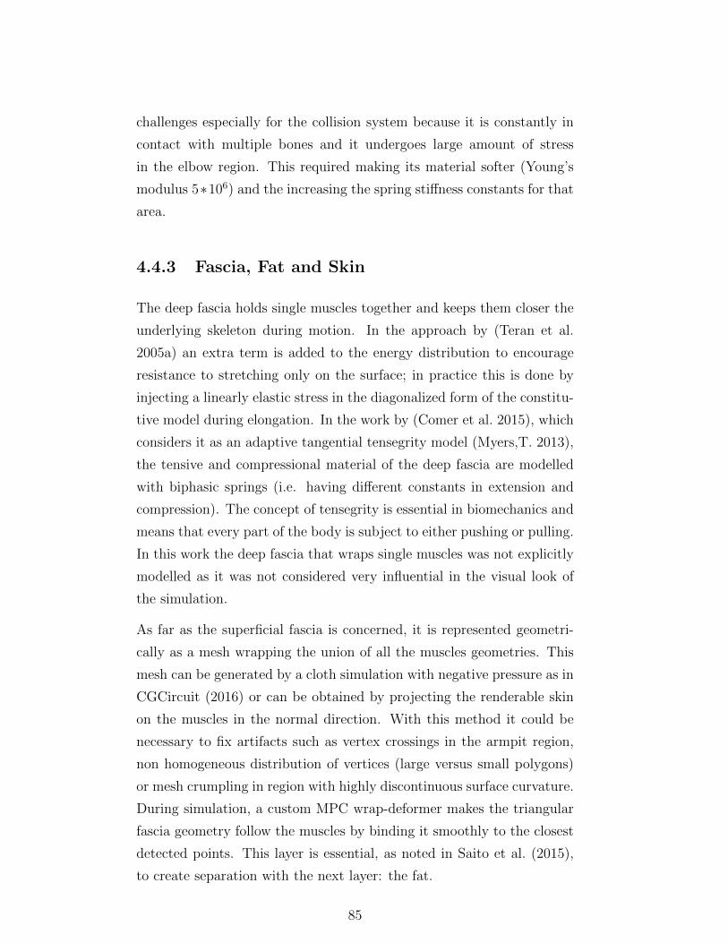
challenges especially for the collision system because it is constantly in
contact with multiple bones and it undergoes large amount of stress
in the elbow region. This required making its material softer (Young’s
modulus 5∗106) and the increasing the spring stiffness constants for that
area.
4.4.3 Fascia, Fat and Skin
The deep fascia holds single muscles together and keeps them closer the
underlying skeleton during motion. In the approach by (Teran et al.
2005a) an extra term is added to the energy distribution to encourage
resistance to stretching only on the surface; in practice this is done by
injecting a linearly elastic stress in the diagonalized form of the constitu-
tive model during elongation. In the work by (Comer et al. 2015), which
considers it as an adaptive tangential tensegrity model (Myers,T. 2013),
the tensive and compressional material of the deep fascia are modelled
with biphasic springs (i.e. having different constants in extension and
compression). The concept of tensegrity is essential in biomechanics and
means that every part of the body is subject to either pushing or pulling.
In this work the deep fascia that wraps single muscles was not explicitly
modelled as it was not considered very influential in the visual look of
the simulation.
As far as the superficial fascia is concerned, it is represented geometri-
cally as a mesh wrapping the union of all the muscles geometries. This
mesh can be generated by a cloth simulation with negative pressure as in
CGCircuit (2016) or can be obtained by projecting the renderable skin
on the muscles in the normal direction. With this method it could be
necessary to fix artifacts such as vertex crossings in the armpit region,
non homogeneous distribution of vertices (large versus small polygons)
or mesh crumpling in region with highly discontinuous surface curvature.
During simulation, a custom MPC wrap-deformer makes the triangular
fascia geometry follow the muscles by binding it smoothly to the closest
detected points. This layer is essential, as noted in Saito et al. (2015),
to create separation with the next layer: the fat.
85

The tetrahedral fat layer is obtained using MPC’s Kali toolset as the
volumetric offset space between the fascia and the skin. It is driven
by the fascia and attached to it via soft sliding constraints (zero-length
springs) distributed regularly. Its typical jiggly behaviour is modelled
using a passive isotropic material (StVK in the examples).
Figures 4.17 and 4.19 show the interaction of all the 3 layers together
(please refer also to the videos at http://www.fabioturchet.com/supplemental_
material.zip). In red colour are the simulated muscles, in yellow the
wrapped fascia and in blue the fat/skin layer. The fascia was cached
and serves as driving geometry: there is no coupling because the 3 layers
were simulated separately. As can be seen (and especially in the videos),
the desired sliding effect of the muscles and the bones under the adipose
tissue was obtained, while self-collisions contribute to the lateral bulging
in the folding region of the elbow joint. It is exactly these subtleties and
nuances that make the skin look “alive”. At this point, an optional last
pass for the triangular geometry of the skin on top of the fat layer can
be performed to generate the final renderable mesh with high-resolution
and higher frequency wrinkles (Li & Kry 2014).
This chapter has presented the approach that was taken to the musculo-
skeletal physical simulation of the layered tissues present in a human
arm. Even if this work takes inspiration from the techniques presented
in Teran et al. (2003) and Teran et al. (2005b), there are some differ-
ences. First of all they don’t use a fascia layer to drive the fat, but
directly connect the muscles to the fat geometry which doesn’t highlight
effects such as sliding of the skin over the bones and the muscles. Sec-
ondly they do not integrate dynamics in the muscle simulation, which is
kept quasi-static. In this work instead the framework supports inertial
effects at the solver level and their effect is controllable with material, ac-
tivation and damping parameters. Moreover, muscle-to-muscle collisions
are not explicitly computed in this work and their effect replaced by the
use of sliding spring constraints. On the fat layer instead self-collisions
are computed explicitly with a point/tetrahedron collision test. At the
material level, the material model used in Teran et al. (2003) adopts
86

Mooney-Rivlin equations for the isotropic part, while here STVK is im-
plemented. Lastly, an explicit analytical formulation has been derived
in this work for the fiber-activated constitutive model so that it can be
integrated in modern FEM solvers such as VEGA.
In the next chapter, the creation of a customized version of the same
solver and tools for artists are presented such that the task of placing
anatomical meshes from a template library is made more efficient and
interactive.
87

Figure 4.11: Full arm simulation. View 1.
88

Figure 4.12: Full arm simulation. View 1. (cont.)
89
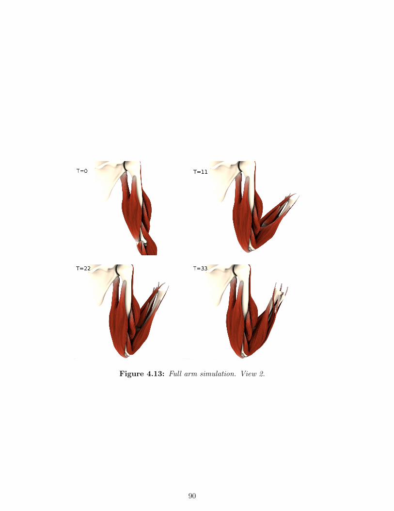
Figure 4.13: Full arm simulation. View 2.
90
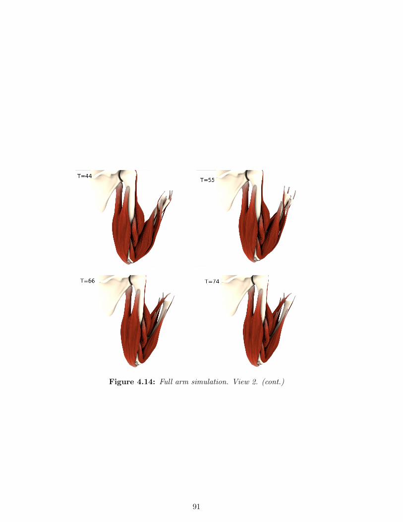
Figure 4.14: Full arm simulation. View 2. (cont.)
91
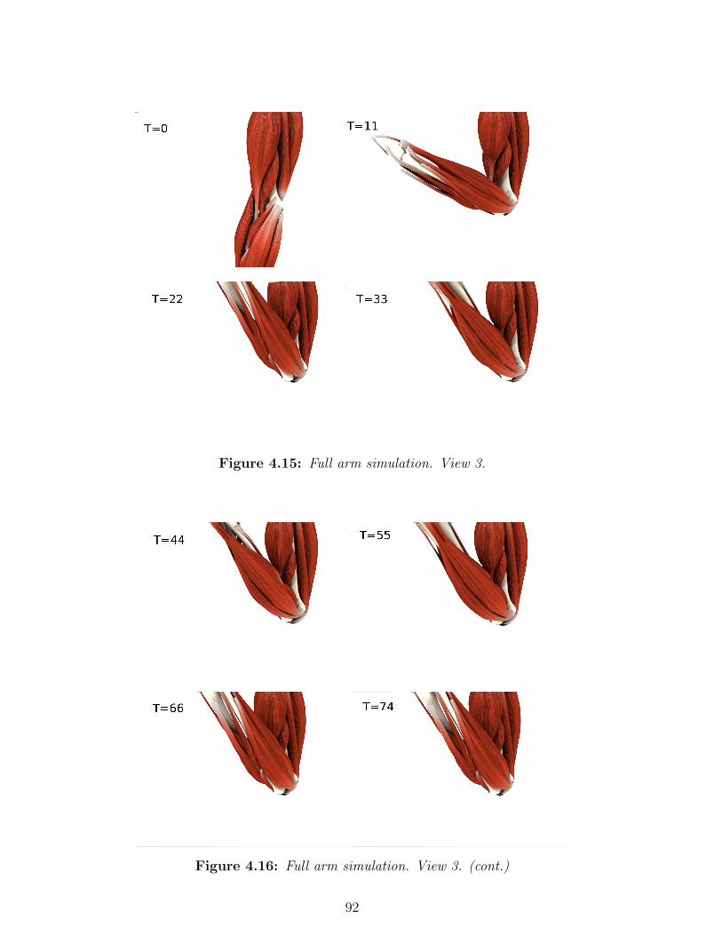
Figure 4.15: Full arm simulation. View 3.
Figure 4.16: Full arm simulation. View 3. (cont.)
92
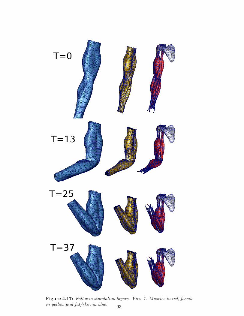
Figure 4.17: Full arm simulation layers. View 1. Muscles in red, fasciain yellow and fat/skin in blue. 93

Figure 4.18: Full arm simulation layers. View 1. Muscles in red, fasciain yellow and fat/skin in blue. (cont.)
94
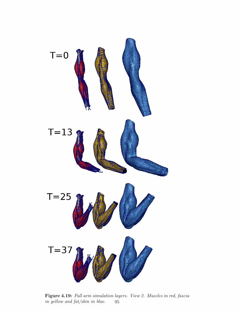
Figure 4.19: Full arm simulation layers. View 2. Muscles in red, fasciain yellow and fat/skin in blue. 95
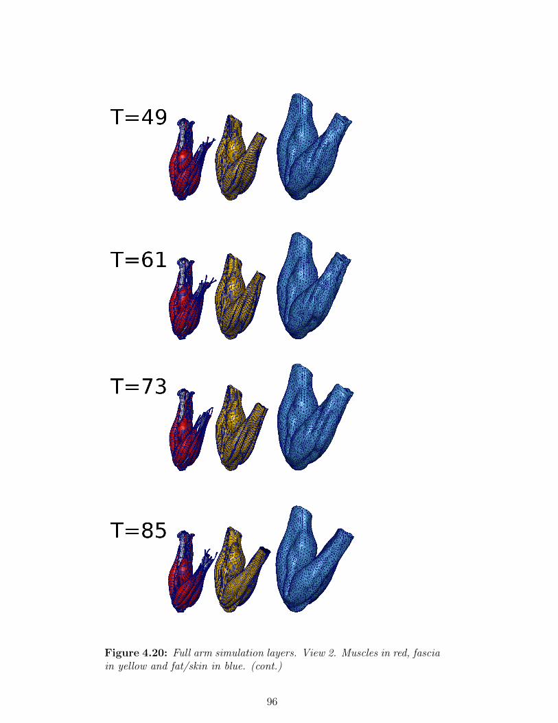
Figure 4.20: Full arm simulation layers. View 2. Muscles in red, fasciain yellow and fat/skin in blue. (cont.)
96
Chapter 5
Muscle Placement
5.1 Introduction
As shown in Chapter 4, one of the main techniques adopted nowadays in
the industry to simulate deformable objects is the Finite Element Method
(FEM). Despite the life-like results, the setup cost to generate and tweak
volumetric anatomical models for a FEM solver is not only very high,
but it cannot easily guarantee the quality of the models either, in terms
of simulation requirements. Unless a system such as the one presented
in Chapter 3 is used, in a production environment in fact models often
require additional processing in order to be ready for FEM simulations
(see section 3.1.1). For example, self-intersections or interpenetrations in
the rest pose may result in unwanted forces from the collision detection
and response algorithms that negatively affect the simulation at its start.
In this chapter a prototype framework and toolset are presented, imple-
mented as a Maya plugin and based on the 3D deformable object FEM
library VEGA (Sin et al. 2013b). The goal is to assist artists and tech-
nical directors (TDs) in the creation of simulation-ready muscle models
in a production environment. Current 3D authoring applications (such
as Autodesk Maya or SideFX Houdini) do not explicitly provide efficient
solutions for this task. Therefore a way to minimise the number of iter-
ations between geometry modelling and production of simulation-ready
97

meshes is proposed, which allows the artist to see the simulated result of
contracting muscles interactively. As a result the efficiency of modelling
targeted to simulation is increased.
5.2 Related Work
Interactivity is a crucial part of any design system that aims to speed
up the artistic process. Existing literature focuses on the application of
fast deformation algorithms to the authoring of deformable objects with
specific desired properties, fast prototyping, design of organic objects
such as vegetation and user control. For example Barbic et al. (2012)
propose an animation editing tool leveraging on the power of model
reduction and the computational efficiency of linearized elasticity that
allows the direct manipulation of vertices of a simulated geometry at
any frame with instant adjustment of the full animation in response.
Constraints and physics are respected via a space-time optimization.
One of the main advantages of interactive methods is that they amplify
the creative possibilities of the artists by allowing the exploration of a
vast space of designs in a short time and provide instant feedback on the
constraint choices. One example of this characteristic is represented in
the work by Xu et al. (2015b) in which the user can design nonlinear
isotropic and anisotropic materials for soft-body simulation intuitively
and interactively by editing spline curves in an interface. The system
works by expressing internal forces and a stiffness matrix in the space of
principal stresses (the singular values of the deformation gradient F) and
using separable strain elastic energies. As a result this gives much free-
dom in the definition of material properties because the user directly edits
the stress/strain curve. Xu et al. (2015a) instead use model reduction
to greatly increase optimization speed while calculating heterogeneous
material properties for deformable objects. The user specifies desired
displacements and internal forces which allows the calculation for exam-
ple of accurate contact forces in fabrication (inverse) design. This means
that the user is freed from the tedious work of setting material param-
98

eters and can instead follow a goal-oriented approach ’starting from the
end’: the optimization will take care of finding the physical parameters
that during simulation lead to the desired result. Similarly, Xu & Barbic
(2017) describes a method to design example-based linear or nonlinear
damping properties for a simulation, by controlling a spline curve.
An interesting complex application of interactive design is represented
by vegetation. Similar in spirit to this work’s goal to produce simulation-
ready meshes, Zhao & Barbic (2013) propose a method that applies do-
main decomposition to the processing of a polygonal “soup” representing
a tree and outputs separated geometries ordered in hierarchy for fast sim-
ulation with minimal user input. From a user selection of triangles into
basic classes, the system automatically builds a domain graph and uses
model reduction for a fast authoring of simulated plants, including pre-
decided fracturing. Hadrich et al. (2017) produce stunning results for
climbing plants authoring using a meshless based representation, specif-
ically anisotropic oriented particles. In this way the system is not only
very fast because of its parallelism, but also supports a multitude of
operation such as bending, breaking, physically and biologically based
growth. Using a similar method, Pirk et al. (2017) propose a system for
the interactive simulation and artistic control of wood combustion for
botanical tree models.
Recently, neural networks and, specifically, conditional generative ad-
versarial networks have also been applied to help artists accelerate the
design process (Guerin et al. 2017), opening a promising new direction
for the application of machine learning in Visual Effects.
5.3 Method
A typical workflow in the system presented in this chapter consists of
the following macro steps (illustrated in Figure 5.1):
• Import of an existing muscle template from a library of meshes or
existing muscle rigs;
99
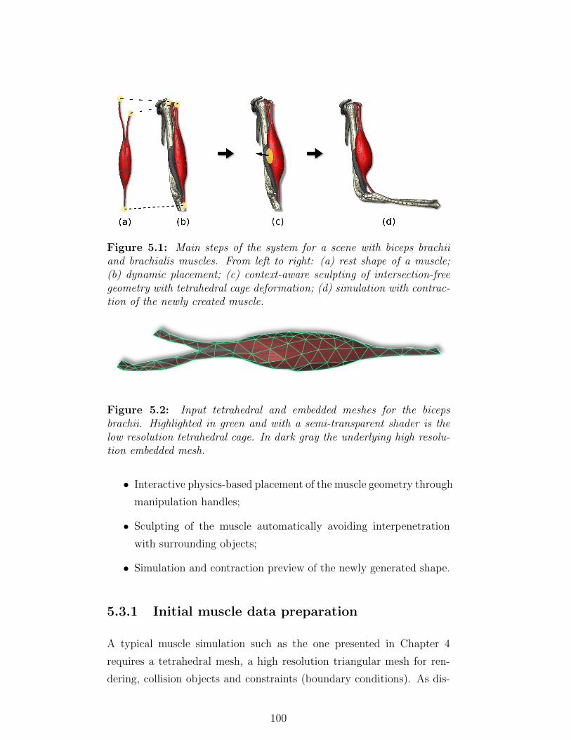
Figure 5.1: Main steps of the system for a scene with biceps brachiiand brachialis muscles. From left to right: (a) rest shape of a muscle;(b) dynamic placement; (c) context-aware sculpting of intersection-freegeometry with tetrahedral cage deformation; (d) simulation with contrac-tion of the newly created muscle.
Figure 5.2: Input tetrahedral and embedded meshes for the bicepsbrachii. Highlighted in green and with a semi-transparent shader is thelow resolution tetrahedral cage. In dark gray the underlying high resolu-tion embedded mesh.
• Interactive physics-based placement of the muscle geometry through
manipulation handles;
• Sculpting of the muscle automatically avoiding interpenetration
with surrounding objects;
• Simulation and contraction preview of the newly generated shape.
5.3.1 Initial muscle data preparation
A typical muscle simulation such as the one presented in Chapter 4
requires a tetrahedral mesh, a high resolution triangular mesh for ren-
dering, collision objects and constraints (boundary conditions). As dis-
100

cussed before in Chapter 4, a mesh for rendering is embedded by using
barycentric coordinates or similar methods and collision objects can be
either rigid, for example, geometry for bones, or deformable, i.e. other
muscle geometry. In addition, the tetrahedral mesh contains volumetric
vector attributes such as a fibre field, continuum mechanics materials
and activation levels used during contraction.
The system assumes the existence of a template library of pre-sculpted
anatomical models of bones, muscles and skin (Figure 5.2). The source
models for the library can be taken from commercially available collec-
tions, as well as reconstructed from freely available medical MRI/CAT
scans and muscles from existing characters. This work makes use of an
adapted 3D model from (CGCircuit 2016) which in turn builds on the
scans of real subjects.
5.3.2 Muscle placement
Once the model is selected from the library, the muscle placement stage
begins. The goal here is to place muscle attachments of the template
model near the bones via an interactive user-controlled simulation. Mus-
cle attachments are sets of vertices (typically of the tendon geometry)
hard-constrained to a driving handle mesh (such as a simple sphere).
One of the main features of this system is that it solves for collisions
with nearby muscles and bones during the placement process, elastically
adapting the muscle to preserve its volume. In this way the framework
differs from standard 3D modelling tools which do not provide these fea-
tures and which result in plastic deformations that can hardly produce
a simulation-ready mesh.
To control the placement, the user can add hard constraints on specified
nodes of the mesh which serve as 6-DOFs manipulators. In the inte-
grator, which implements Implicit Backward Euler (Eq. 4.4), the con-
strained nodes inherit position and velocity of these manipulators, rather
than being directly solved. This produces a change of the deformation
gradient that triggers elastic deformation. Rayleigh stiffness damping
101
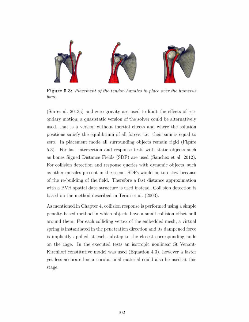
Figure 5.3: Placement of the tendon handles in place over the humerusbone.
(Sin et al. 2013a) and zero gravity are used to limit the effects of sec-
ondary motion; a quasistatic version of the solver could be alternatively
used, that is a version without inertial effects and where the solution
positions satisfy the equilibrium of all forces, i.e. their sum is equal to
zero. In placement mode all surrounding objects remain rigid (Figure
5.3). For fast intersection and response tests with static objects such
as bones Signed Distance Fields (SDF) are used (Sanchez et al. 2012).
For collision detection and response queries with dynamic objects, such
as other muscles present in the scene, SDFs would be too slow because
of the re-building of the field. Therefore a fast distance approximation
with a BVH spatial data structure is used instead. Collision detection is
based on the method described in Teran et al. (2003).
As mentioned in Chapter 4, collision response is performed using a simple
penalty-based method in which objects have a small collision offset hull
around them. For each colliding vertex of the embedded mesh, a virtual
spring is instantiated in the penetration direction and its dampened force
is implicitly applied at each substep to the closest corresponding node
on the cage. In the executed tests an isotropic nonlinear St Venant-
Kirchhoff constitutive model was used (Equation 4.3), however a faster
yet less accurate linear corotational material could also be used at this
stage.
102
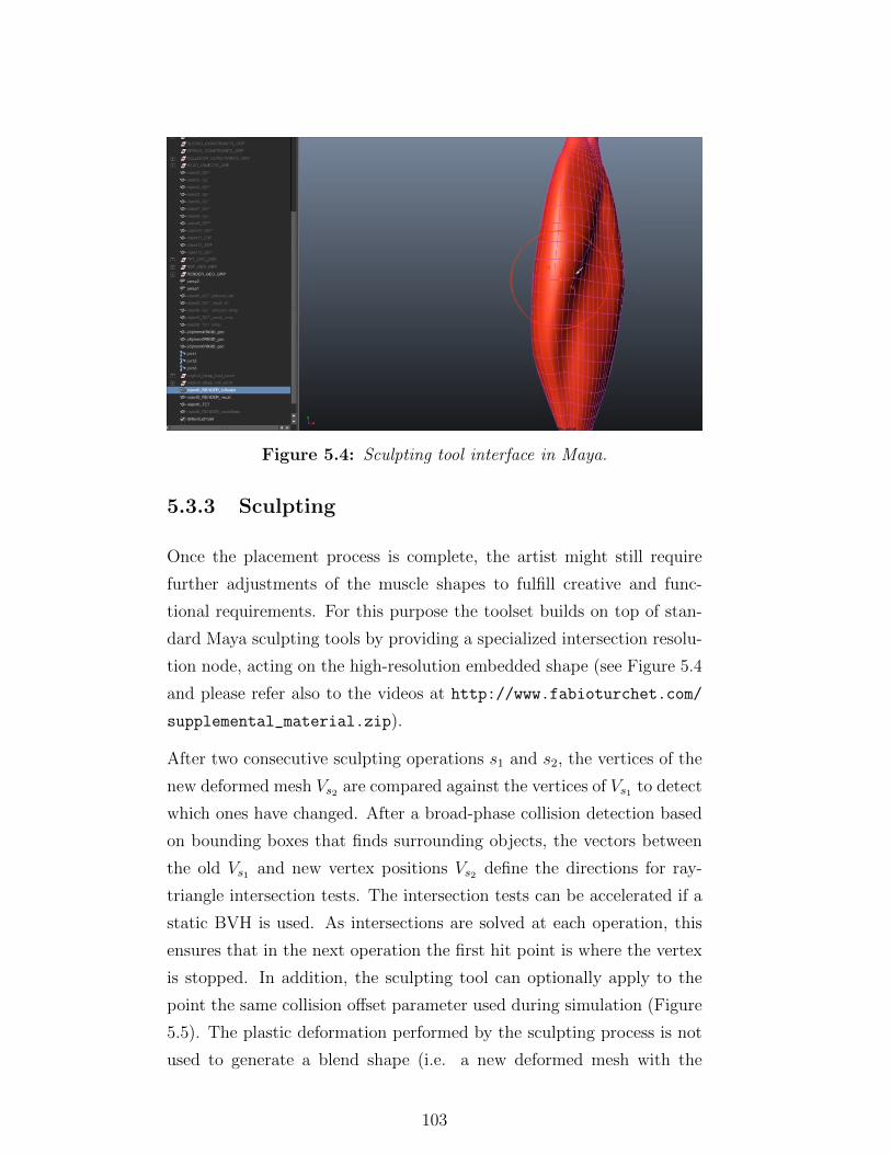
Figure 5.4: Sculpting tool interface in Maya.
5.3.3 Sculpting
Once the placement process is complete, the artist might still require
further adjustments of the muscle shapes to fulfill creative and func-
tional requirements. For this purpose the toolset builds on top of stan-
dard Maya sculpting tools by providing a specialized intersection resolu-
tion node, acting on the high-resolution embedded shape (see Figure 5.4
and please refer also to the videos at http://www.fabioturchet.com/
supplemental_material.zip).
After two consecutive sculpting operations s1 and s2, the vertices of the
new deformed mesh Vs2 are compared against the vertices of Vs1 to detect
which ones have changed. After a broad-phase collision detection based
on bounding boxes that finds surrounding objects, the vectors between
the old Vs1 and new vertex positions Vs2 define the directions for ray-
triangle intersection tests. The intersection tests can be accelerated if a
static BVH is used. As intersections are solved at each operation, this
ensures that in the next operation the first hit point is where the vertex
is stopped. In addition, the sculpting tool can optionally apply to the
point the same collision offset parameter used during simulation (Figure
5.5). The plastic deformation performed by the sculpting process is not
used to generate a blend shape (i.e. a new deformed mesh with the
103
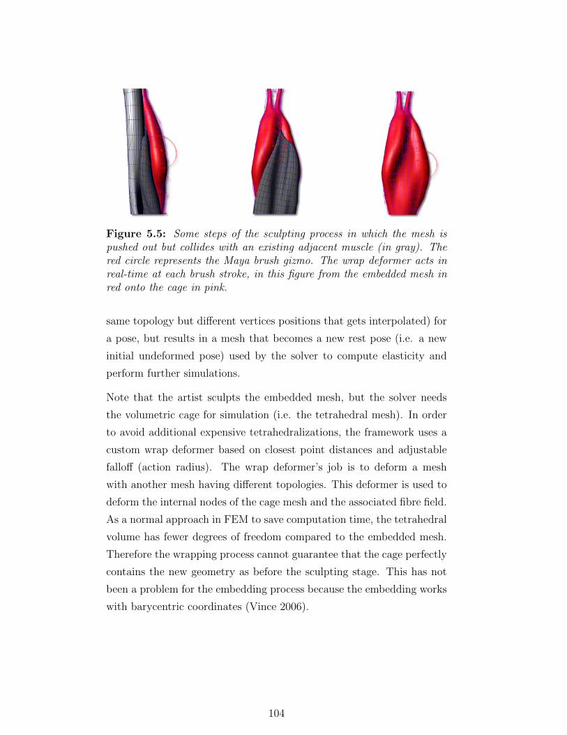
Figure 5.5: Some steps of the sculpting process in which the mesh ispushed out but collides with an existing adjacent muscle (in gray). Thered circle represents the Maya brush gizmo. The wrap deformer acts inreal-time at each brush stroke, in this figure from the embedded mesh inred onto the cage in pink.
same topology but different vertices positions that gets interpolated) for
a pose, but results in a mesh that becomes a new rest pose (i.e. a new
initial undeformed pose) used by the solver to compute elasticity and
perform further simulations.
Note that the artist sculpts the embedded mesh, but the solver needs
the volumetric cage for simulation (i.e. the tetrahedral mesh). In order
to avoid additional expensive tetrahedralizations, the framework uses a
custom wrap deformer based on closest point distances and adjustable
falloff (action radius). The wrap deformer’s job is to deform a mesh
with another mesh having different topologies. This deformer is used to
deform the internal nodes of the cage mesh and the associated fibre field.
As a normal approach in FEM to save computation time, the tetrahedral
volume has fewer degrees of freedom compared to the embedded mesh.
Therefore the wrapping process cannot guarantee that the cage perfectly
contains the new geometry as before the sculpting stage. This has not
been a problem for the embedding process because the embedding works
with barycentric coordinates (Vince 2006).
104

Figure 5.6: Some steps of the simulation process, in which the bendingof the elbow joint activates the contraction of the biceps brachii.
5.3.4 Simulation
Once the new sculpted muscle is completed, the barycentric coordinates
have to be recomputed and the solver is re-initialized with the new tetra-
hedral mesh rest shape to preview the contraction of the muscle in an
animation. In the simulation step the same solver as in the muscle place-
ment stage is used, which allows the integration of the same data struc-
tures seamlessly as a part of the same framework.
The muscle material can be changed from a pure isotropic material to a
transversely isotropic material that makes use of the fibre directions field.
In particular, as discussed in Chapter 4 the constitutive model presented
in Teran et al. (2003) was implemented, with active and passive stress
response, with different Young modulus for tendons and muscle body
materials. In the simulation stage the system supports not only hard
constraints, but also soft and sliding constraints. This allows the creation
of the interconnected network of connective tissue known as fascia which
keeps the muscles packed together during motion.
5.4 Implementation and Results
The solver and the sculpting tool are implemented as C++ multi-threaded
Maya plugins. The solver extends the Maya class MPxNode. Its in-
put connections are a time node, the tetrahedral and embedded meshes
105
and various parameters such as gravity vector, iterations number, self-
collisions flag which are editable from Maya’s Attribute Editor. Its out-
put is the tetrahedral mesh. Every time one of the inputs changes, the
node graph is recomputed and the compute function of the solver is
called, executing a timestep. Other solver parameters such as the ma-
terial model are contained in an input file specific to each deformable
object which follows VEGA’s configuration file format. The sculpting
tool also extends MPxNode and executes at any mesh editing operation
performed by the user for instance using the Artisan sculpting toolbox
and brushes. The wrap deformer node mentioned in this chapter is the
standard one available in Maya. The initial tetrahedralization is per-
formed using TetGen and is stored in .veg files, while the SDFs are stored
using OpenVDB. The code can be greatly optimized performance-wise.
For simplicity, the prototype was tested on a basic two-muscles setup in
which a user places biceps brachii over brachialis by moving constraint
handles attached to each tendon end. In a real use case the scene could
contain many muscles that would be placed in layers from the internal
to the most external ones. This would not considerably affect the perfor-
mance because the existing placed muscles would be kept as static rigid
objects and only the data structure for collisions would grow in size.
Performance would drop if multiple muscles would be moved at once.
For the placement part the material used is the isotropic StVk, while
for the contraction preview it switches to anisotropic. After the bicep
is placed by translating and rotating its handles in a position which
resembles its real anatomical position on the character, the user sculpts
its central body by making it much bigger and finally previews its new
shape in an animation that activates the contraction (5.6).
In terms of performance, one muscle made of 400 tetrahedra, subject to
15 hard constraints and 100 collision constraints, interacting with one
bone and one other muscle, can be placed interactively at ∼15 fps using
a timestep of 0.01s. Because the accuracy in this kind of design appli-
cations is secondary over performance, the parameter or the maximum
number of iterations performed by the PCG solver was kept low (10-20).
106

The next chapter presents a procedural technique based on continuous
scalar fields that doesn’t use physics, but allows the addition of wrinkles
as a post-process effect.
107

Chapter 6
Implicit Skinning Extension
6.1 Introduction
Figure 6.1: Overview of the workflow of the system. (a) Angle fieldgradients; (b) Seeds and curves; (c) Final result (meshes are subdivided);(d) Real example of a left thumb.
Skinning is one of the most important areas in the field of computer
animation and visual effects, where character realism and believability
are essential. A large number of methods exist and are implemented in
modern animation systems (Gain & Bechmann 2008). One of the recent
advancements in the area which produces believable results is the Implicit
Skinning technique (Vaillant et al. 2013). Unlike other methods which
only use surface (vertices and triangles) data, Implicit Skinning makes
use of implicitly-defined continuous scalar fields, in particular Hermite
Radial Basis Functions (HRBF). This helps in solving the drawbacks
that linear blend skinning and dual quaternion skinning exhibit: loss of
volume, lack of collisions and unwanted bulging.
During animation, the fields associated with each skeleton bone are
108

rigidly transformed and the mesh vertices march in the direction of the
gradient of the combined field until they reach the isovalue they had in
the rest pose. This allows better preservation of the initial shape and
better deals with self collisions in the folding region, either by stopping
the marching at gradient discontinuities or by using a contact operator
(Vaillant et al. 2014). The framework also allows the creation of interest-
ing effects through the use of gradient-based operators, for example the
bulge in contact which approximates volume preservation. Nevertheless,
to the author’s knowledge, important secondary effects such as wrinkling
have not been previously investigated for this technique.
In this chapter it is described the extension of implicit skinning to gen-
erate plausible and temporally-coherent wrinkles for skeleton-driven 3D
animated characters. The technique benefits from the available trans-
formed scalar fields: from their interaction a vector field that resem-
bles plausible wrinkle directions is generated, hence creating a hybrid
polygon-implicit approach.
The main contributions of this work are:
1. A technique for the creation of wrinkle curves based on the implicit
skinning method.
2. A large set of parameters to allow users to procedurally tune the
behaviour of the wrinkles and thus obtain the desired result.
6.2 Related work
Despite being considered a secondary effect in skin simulation systems
(Clutterbuck & Jacobs 2010), wrinkling has been attracting the attention
of both academia and industry as an important detail to add realism to
Computer Generated (CG) characters. Elastic thin sheets like cloth or
skin create wrinkles when compression forces are applied, to preserve
material and isometry (the property of being inextensible) of the rest-
pose object.
Current approaches can be categorized as artist-driven, in which drawn
109
wrinkles maps are blended (Jimenez et al. 2011), procedural, based on
textures (Kimmerle et al. 2004), and physics based, often using a bend-
ing energy formulation in a specialized cloth solver (Bridson et al. 2003).
An accurate way to measure stretching and compression is via the stretch
tensor as presented in Rohmer et al. (2010). Their work is focused on
augmenting coarse mesh cloth simulations with fine details such as wrin-
kles and refining the tessellation in localized areas through adaptivity.
The rest mesh is parametrized to a plane in order for the triangles to
have a common frame of reference and the stretch tensor is calculated as
defined in (Talpaert 2010). This is then diagonalized and its eigenvalues
and eigenvectors give the magnitude and direction of the wrinkle vector
field, respectively. Wrinkles are then generated as convolution surfaces
from this field’s streamlines by growing curves from seeds with the high-
est vector magnitude. The technique presented in this chapter follows
the same procedural approach for curve generation but substitutes the
stress field by the gradient of a scalar angle field, without using planar
parametrization. In this way the properties of the fields are exploited
instead of calculating the stress tensor.
Recent works on skin in particular make use of physics-based simulation.
Remillard & Kry (2013) presents an approach in which thin shells are
embedded in coarser finite element meshes to simulate the wrinkling ef-
fects of hard skin surrounding soft objects. The key idea is the use of
frequency based position constraints, modelled as discretized continuous
functions, that allow wrinkle formation only at wavelengths matching
physical material properties. The work by Li & Kry (2014) extends this
technique by adding multi-layer support for heterogeneous materials and
creating extremely fine and realistic skin details trough the use of adap-
tive meshes, for which normal or displacement maps can be exported.
Warburton (2014) in his work successfully applies a variation of the Fi-
nite Element method to the simulation of realistic forehead wrinkles on
the GPU. Wrinkles as part of a larger simulation framework were pre-
sented in Weta’s proprietary Tissue system (WETA Digital 2013) that
uses finite elements to simulate fascia/fat/skin layers and constraints to
solve wrinkling problems.
110
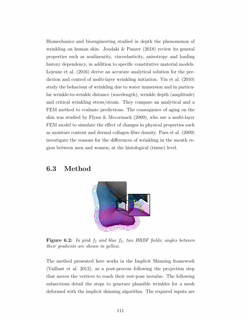
Biomechanics and bioengineering studied in depth the phenomenon of
wrinkling on human skin. Joodaki & Panzer (2018) review its general
properties such as nonlinearity, viscoelasticity, anisotropy and loading
history dependency, in addition to specific constitutive material models.
Lejeune et al. (2016) derive an accurate analytical solution for the pre-
diction and control of multi-layer wrinkling initiation. Yin et al. (2010)
study the behaviour of wrinkling due to water immersion and in particu-
lar wrinkle-to-wrinkle distance (wavelength), wrinkle depth (amplitude)
and critical wrinkling stress/strain. They compare an analytical and a
FEM method to evaluate predictions. The consequence of aging on the
skin was studied by Flynn & Mccormack (2009), who use a multi-layer
FEM model to simulate the effect of changes in physical properties such
as moisture content and dermal collagen fibre density. Paes et al. (2009)
investigate the reasons for the differences of wrinkling in the mouth re-
gion between men and women, at the histological (tissue) level.
6.3 Method
Figure 6.2: In pink f1 and blue f2, two HRBF fields; angles betweentheir gradients are shown in yellow.
The method presented here works in the Implicit Skinning framework
(Vaillant et al. 2013), as a post-process following the projection step
that moves the vertices to reach their rest-pose isovalue. The following
subsections detail the steps to generate plausible wrinkles for a mesh
deformed with the implicit skinning algorithm. The required inputs are
111
therefore the continuous scalar fields of the segmented mesh of which
value and gradient are used.
The method is based on the post-processing technique presented by
(Rohmer et al. 2010). The difference with their approach is that here the
stretch tensor is replaced with a discrete scalar field calculated from the
single fields associated with each bone. Its value at each vertex is defined
as the angle between the gradients of two adjacent fields. This avoids
the parametrization of the mesh in planar space while taking full advan-
tage of the implicitly-defined scalar field. The key observation is that
the gradient of this angle field resembles the direction in which human
skin wrinkles in bending fingers or arms.
6.3.1 Angle Fields Preparation
The vector field representing wrinkle directions, constrained on the sur-
face, is a gradient field of the discrete scalar angle field and it is calculated
by taking the finite differences in the local frame of each vertex. In prac-
tice, for production-ready meshes, it can be approximated by taking the
finite differences on the one-ring neighbours of the vertex, as described
below.
The generation of a discrete scalar field for each pair of adjacent joints
in the skeleton hierarchy will now be defined formally. Let f1 and f2
be two consecutive fields with compact support. During animation of a
bending joint chain f1 and f2 will rotate rigidly towards each other. For
each vertex in f1 ∩ f2 the angle between the gradients of f1 and f2 can
be calculate straightforwardly as (see Figure 6.2):
angle(f1, f2) = arccos(∇f1 · ∇f2
)where gradient vectors are assumed to be normalised.
Once an angle field fA is defined, its gradient is approximated with finite
differences by searching in the one-ring neighbours the position with
112

minimum value pmin. For a source vertex p the gradient is then:
∇fA = pmin − p
In practice, the user can choose to use a version of this field in which the
gradients are biased towards one of the connected edge vectors. Based on
the quality of the deformed topology, in this way more regular anisotropic
patterns can be achieved if desired (Figure 6.3. To generate fields less de-
pendent on the mesh resolution the search can be done in ring neighbours
of levels greater than one, which are pre-stored for efficiency. Consider-
ing three hierarchical fields f1, f2 and f3 in which f2 is child of f1 and
f3 child of f2, they can interoperate in such a way that f1 can create
wrinkles with field f2, but not with f3.
6.3.2 Curve Creation
The wrinkle curves are grown from the potential seeds selected from
the vertices satisfying the user-controlled parameters and which are pro-
cessed in a priority queue based on their associated angle. For each new
seed a curve is grown in both the directions determined by the maximum
gradients of its surrounding neighbours. Temporal coherence is achieved
by keeping curves from the previous frame and deleting them if their
corresponding seeds do not satisfy specific criteria for the current frame.
Depending on the extension of the local support of the implicit skinning
fields, wrinkles could also appear both in the rest pose and on undesired
regions of the mesh. This problem is solved by creating a seed only
if the corresponding joint is bent more than a specified threshold. In
addition, a subset of the initial vertices is precomputed by excluding
those not in the folding region. This is obtained by thresholding based
on the dot product between the vertex normal and the up vector of the
associated bone’s local rotation frame. Finally, the vertices forming a
curve are displaced in their normal direction by a controllable amount.
This approach works for both static frames and animations.
At each frame every vertex is processed and inserted in a priority queue
113

based on its angle value. The curve generation algorithm begins by
selecting a seed from the top of the queue (red dots in Figure 6.6(d));
starting from it, vertices are added to the curve by iteratively choosing
the next candidate in the one-ring neighbourhood N that has edge vector
most similar to the gradient of the field at the source point. This process
is repeated for the newly added point.
As in (Rohmer et al. 2010) the curve is grown in both directions, with
the addition that for each seed we invert the gradient at that point to
grow the second half of the curve. By indicating with q a candidate
neighbour and by e = q − p the edge vector, the next vertex to add to
the curve is calculated as:
pnext = minq∈N
(arccos(e · ∇fA))
after normalizing vectors in arccos. The generated angle field has gradi-
ents pointing in plausible wrinkles directions because the angles decrease
moving further away from the folding region, where their values are sim-
ilar to the joint bending angle.
Every time a new point is added, its Euclidean distance is checked against
all the current curves to enforce the constraint that all of them must stay
at a minimum user-defined distance. The curve points loop terminates
when a point’s angle is under a user-set threshold or when it ends up
outside of the allowed internal region of the mesh. Due to the fact that
for dense meshes the number of curve points can be high and would nega-
tively influence performance, a resampling of the curve can be performed
which in practice corresponds to a simple pruning.
In order to maintain temporal coherence between consecutive frames, the
active curve list is kept from one frame to another and a curve removed
from it if its corresponding seed ends up outside one of the associated
fields, which can be defined by checking the isovalue against the thresh-
old. Therefore the curves are not grown again from their associated seed
after they are generated. This is in line with the observation that for
human skin in particular, wrinkles tend to form at the same position
for multiple repetitions of the same movement (fingers are a typical ex-
114

ample), a feature exploited for instance by Cao et al. (2015) for their
wrinkle likelihood map generation.
During animation, fields rigidly rotate and interpenetrate one another
which causes configurations for which a field (the one associated to a
finger phalanx for example) happens to be “immersed” into another field.
This becomes problematic because seeds will be selected from the whole
mesh segment and wrinkles would appear in unwanted regions, like the
nail. Therefore, as a precomputation step, only the vertices on the same
side of the joint bending direction are selected for wrinkle generation.
This is done easily by thresholding based on the dot product between the
vertex normal and the up vector of the associated bone’s local rotation
frame.
6.3.3 Wrinkle Field
The curves created as described in section 6.3.2 are a set of line segments
connecting vertices of the mesh. These segments are transformed into
convolution surfaces wi and the sum of their field contributions gets
thresholded:
vwrinkles =∑i
(wi)− T
In this method the convolution surfaces used are with line segments as
skeletons and Cauchy kernel as a potential function. This surface for
line segment with position vector ai, normalized direction di and length
l has the following closed-form formulation (McCormack & Sherstyuk
1998):
wi(x) =n
2p2(p2 + s2n2)+l − n2p2q2
+1
2sp3(atan[
sn
p] + atan[
s(l − n)
p])
where n = (x− ai) · di, p2 = 1 + s2(|x− ai|2 − n2) and q2 = 1 + s2(|x−ai|2 + l2 − 2ln)
The following default parameters (empirically chosen) are used for the
convolution surface: T = 0.5 and s = 0.85.
The advantage of using convolution surfaces is that the segments smoothly
115

blend-in and they can be integrated straightforwardly with the existing
HRBF fields. Because there is no stretch information per face in this
method, the radius of each segment gets modulated by a factor that
depends on the angle magnitude at each curve point. This in general
makes the wrinkle thicker at the center of the field and smoothly nar-
rower at the edges. For fast value query each segment’s bounding box is
also inserted in a KD-tree.
6.3.4 Projection
After obtaining vertex positions from the last step of implicit skinning
and wrinkle fields vwrinkles, the HRBF field and wrinkles field are com-
bined. Thus, the value vcomb at an arbitrary point pw is:
vcomb(pw) = max(vHRBF (pw)− 0.5, vwrinkles(pw))
It can be seen that here a simple set-theoretic operation is used, yet more
complex blend operators can be adopted as well. Vertices get projected
to this combined field by using Newton’s iterations (Figure 6.4). Dur-
ing projection collisions are not calculated using gradient discontinuities.
Instead, to avoid evident mesh interpenetrations, the smoothing coeffi-
cients generated in the main implicit skinning step are reused to exclude
from the displacement the vertices in the colliding folding region.
Unfortunately the equivalence between the decomposed stretch tensor’s
eigenvalues and the angles magnitude cannot be used to activate the
wrinkles because already in the rest-pose the angle values are not zero
and during animation noisy fluctuations in the angle field are experi-
enced. Therefore, in order to produce a smooth appearance for the
wrinkles, the depth of the curve is modulated by the offset between
the current and the rest-pose’s joint activation angles, in a fashion sim-
ilar to how a pose-based deformation works. The gradual appearance
is achieved by placing the curve vertices initially under the surface at
a distance R corresponding to the radius of the segment and smoothly
moving them upwards in the normal direction.
116

For fast preview purposes, a simplified procedure can be applied. Instead
of projecting the vertices to the wrinkles field, a simple displacement of
the vertices corresponding to the curve points can be executed. However
in this case the wrinkles radius is not controllable and wrinkles appear
to be too sharp and uniform.
6.3.5 Parameters
The presented system is procedural and allows the user to control the
appearance of the wrinkles by tweaking basic parameters (see Figure
6.5), some of which are described below (please refer also to the videos
at http://www.fabioturchet.com/supplemental_material.zip).
Wrinkle Radius: the base radius for the convolution surfaces
Direction Threshold: the minimum angle that the gradients at two
consecutive points of a curve must form. This parameter helps to achieve
a more organic look and longer wrinkles as it allows the curves to be
approximately straight.
Seed Angle Threshold: the minimum angle that a seed point must
have to be selected. This allows wrinkles to also start forming at the
edges.
Field Threshold: minimum isovalue that a seed vertex must have to
be selected
Angle Threshold: the minimum angle that any curve point must have;
this controls the termination of the curve growth process
Seed Distance: keeps the seeds at a minimum Euclidean distance
Displace Strength: controls how deep the convolution surfaces stay
under the mesh so as to modulate bigger or smaller displacements
Ramp Control: a smooth spline that controls how fast and linear the
wrinkle appearance is
Appearance Time: activation time, expressed in frames or joint angle
degrees
Topology Bias: this parameter forces the angle field calculation to
examine only the connected vertices.
117
6.4 Implementation and Results
The method is implemented as a C++ Maya 2015 plugin. Both value and
gradient of the rest-pose HRBF fields are stored as OpenVDB textures
because their evaluation is computationally too expensive as it requires
solving a linear system per frame. This means that at each frame the
HRBF field is not recomputed but the inverse matrix of the joint trans-
formations is used instead to read the value in the rest-pose.
As the angle calculation is independent per vertex, this step can be
parallelized. The angle field computation and the vertex projection are
in fact multi-threaded, but could also be implemented on the GPU, for
example using the Fabric Engine framework (Fabric Engine 2015). The
code could be further optimized, but performance highly depends on the
number of iterations in the projection steps which in turn determines the
number of accesses to the textures. On a quad-core Intel Xeon X3470
machine, for the thumb mesh with 15K vertices, 15 curves and 4 joints
the framerate is ∼ 10fps (including implicit skinning projection and
smoothing).
Tests of the technique were conducted mainly on cylindrical objects such
as fingers, arms and legs and achieved believable results. Figure 6.6 shows
the detail of a thumb which is particularly interesting due to the various
wrinkle patterns of different sizes. This example uses constant radius
and the field used is the non biased one: note how the curves develop
independently of the mesh connectivity because of the higher degree of
freedom in terms of possible neighbour directions.
Even though the technique does not always produce full wrinkle curves
from one edge of the finger to the other (due to discontinuities or noise in
the field), it still creates an organic and believable look. Note the use of
the smoothing coefficients to avoid wrinkle displacement where vertices
collide (Figure 6.6 (e)). The patterns are comparable to a real example
(Figure 6.6 (f)). Moreover, close wrinkles are blending in quite naturally
because of the convolution surfaces formulation. Figure 6.7 shows com-
parative results between biased and non biased fields for the mesh of an
118

arm: the topology-biased field produces more believable wrinkles.
In some cases unwanted bulges can appear: this is due to curves which are
too short or whose curvature is too high in some of their segments. This
could be addressed by filtering out these cases from the final used set. In
addition, it was noticed that the 3D texture resolution can strongly con-
dition the quality of the angle fields due to interpolation approximations.
In general better results were achieved using 4 or more ring-neighbour
levels, especially for high resolution meshes; even though this improves
the accuracy of the vector field, it also consequently slows down the
system because more vertices have to be processed.
During animation the technique behaves as expected in terms of temporal
coherence, with wrinkle curves that do not pop between frames and slide
thanks to the underlying deformation. If the curves were retraced at each
frame from the seeds, the result would be unstable and non coherent,
mainly because of the differences in two temporally consecutive fields.
Nevertheless, the behaviour of the technique during animation could be
further improved. Dynamic appearance is still not convincing enough,
in fact the wrinkles appear too suddenly: this could be improved by
tweaking the activation curve manually or deriving it from experiments.
Self collisions between the convolution surfaces (using a bulge-in-contact
operator) would also prove beneficial to the overall fleshy look and dy-
namism of the deformation. The reproduction of properties of the skin,
such as the ones due to aging, have not been considered yet and consti-
tute interesting direction for future work.
The validation and evaluation of the technique has been done at the vi-
sual quality level and not through rigorous objective comparisons with
physical based models as some of the work presented in section 6.2. Ac-
curate measurements of visual quality such as local wrinkle density and
height from previous work and from images of real skin would help to
evaluate the model more objectively. To validate the system further at
a more general level, it would be ideal to survey artists feedback in the
testing and reproduction of different wrinkle patterns. The variation
could come from photographs of subjects in different poses and facial
119

expressions of varying gender and age.
In this chapter a technique that allows wrinkles creation within the Im-
plicit Skinning framework has been presented. The technique creates
convenient and plausible results visually similar to the ones obtained
with physically accurate stretch-based methods. The results show the
potential of the technique for applications within a production pipeline.
The next chapter presents the last project of this thesis. Its goal is
to apply machine learning to the simulations of deformable objects in
order to save computation time and substitute the solver in controlled
constrained scenes with a GPU-based Deep Neural Network.
120

(a) Original angle gradient field
(b) Topology-biased gradient field
Figure 6.3: Angle field generation using one-ring neighbours (a) andconnected vertices (b).
121
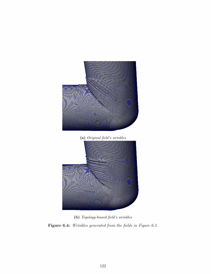
(a) Original field’s wrinkles
(b) Topology-biased field’s wrinkles
Figure 6.4: Wrinkles generated from the fields in Figure 6.3.
122

Figure 6.5: Plugin Parameters.
123
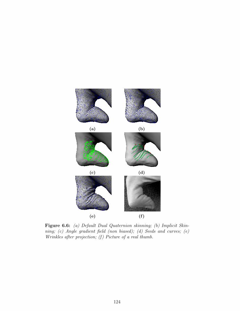
(a) (b)
(c) (d)
(e) (f)
Figure 6.6: (a) Default Dual Quaternion skinning; (b) Implicit Skin-ning; (c) Angle gradient field (non biased); (d) Seeds and curves; (e)Wrinkles after projection; (f) Picture of a real thumb.
124

Figure 6.7: Comparison of the results obtained for an arm. (a)-(d)front and back views using topology biased field; (e)-(h) front and backviews using normal, non biased field.
125

Chapter 7
Pilot Study on Deep Learning
for Deformable Objects
7.1 Introduction
The work presented in this chapter describes how Deep Learning ar-
chitectures can be applied as powerful regressors to the prediction of
physics states for elastic objects, accelerating and potentially substitut-
ing traditional physics solvers. In modern physics-based animation elas-
tic objects are simulated using the Finite Elements Method by solving
Newton’s differential equations of motion in the form of a sparse linear
system. Typically Preconditioned Conjugate Gradient is used for this
task. Even though state of the art methods that are both fast and stable
exist (Bouaziz et al. 2014), a data-driven approach could be a competi-
tive alternative.
The initial purpose of this project was to first understand how to learn a
model to express the dynamics of a physics-based cloth animation with
constraints in the form of a toy problem. After that first stage the goal
was to extend the system to support volumetric (tetrahedral) objects
and apply convolutional neural networks to the learning of constrained
muscle simulation. The motivation driving the project was that a cloth
simulation is in general very detailed and fast changing while muscles
126
deform in a much more stable manner therefore they would be easier to
learn by a machine learning algorithm. It will be shown how solving the
first stage turned out to be very problematic (due for instance to the nov-
elty of application of the geodesic convolution) and the complexity of the
recalculation of one of the inputs of the network hindered the advance-
ment to the second stage for volumetric objects. These challenges paved
the way to an understanding of the main limitations of the proposed
approach and the solutions that will constitute the future work.
7.1.1 Background
Here a brief introduction to neural networks terminology is given for a
much more complete reference please refer to Andrej Karpathy (2017).
A Neural Network (NN) is a set of interconnected units called neurons.
Each neuron’s job is to output a value by multiplying its inputs by a
weights matrix (which constitute the learnable parameters) and passing
the result through an activation function which is nonlinear (examples
are the sigmoid, softMax, tanh, ReLU functions). This nonlinearity is
what allows the network to learn complex real world functions: a NN
can be in fact considered a universal functions approximator which finds
patterns in complex unstructured data.
In terms of architecture, a NN is an acyclic graph and neurons can be
grouped and organized in layers. In a layer connections are not between
the same layer’s neurons, but between layers. When all neurons of one
layer are pairwise connected to the ones of the next layer, it is called
a fully connected layer (FC). Apart from input and output layers, the
ones in the middle are called hidden layers and the fact that they can be
cascaded and be many in number gave rise to the term Deep Learning.
At each layer the network learns to represent internally some features of
the input and deeper layers learn a hierarchical representation of high
level global features. In the case of images of faces for example, in the
early layers simple contrasted edges are detected while in more deep ones
these edges are assembled in more meaningful patterns corresponding
127

Figure 7.1: Lee et al. (2011)
to features such as ear or nose and even further down the full face is
considered as a global abstract feature (Figure 7.1).
A particular kind of NNs are the so called Convolutional Neural Networks
(CNN) created to make the learning of input images very efficient. They
are based on the assumption that an image should be analysed spatially
and not interpreted as a linear vector with no relation between neigh-
bouring pixels. To this end the convolution operation takes the input
and uses filters with kernel weights and extracts the activation of this
filters by sliding them as a window across the image. This operation is
defined mathematically (Goodfellow et al. 2016) and the filter weights
constitute the learnable parameters. The layers of a ConvNet are in 3D
(width, height and depth) and each layer transforms 3D input volumes
to 3D output volumes of neuron activations.
A CNN learns by performing a sequence of forward and backward passes.
The goal of the NN is to minimize a loss function (in literature also called
cost, or objective function) which is peculiar to each problem and rep-
resents the error that should be minimized. In the forward pass the
network takes an input and passes it through its layers; based on the
filters that it learned during training some neurons will be excited and
activate more than others and their contribution will globally produce
an output. For a classifier this could be as simple as telling if an image
belongs to Dogs or Cats classes and with which probability. In the back-
ward pass the actual learning happens (called backpropagation). The
gradient of the loss function with respect to the parameter weights (par-
tial derivatives) is computed given a training input sample and it is used
128

by algorithms such as Stochastic Gradient Descent (SGD) to understand
in which direction the function decreases. ADAM is a very popular vari-
ation of this algorithm (Kingma & Ba 2014). From the output layer back
to the first hidden layer the filter weights are therefore updated in such
a way that the loss function is minimized. This constitutes the training
process and is repeated a certain number of epochs (in an epoch all the
training samples are processed by the network).
One of the main problems when doing machine learning is the risk of a
behaviour commonly called overfitting : this happens when the network
learns the training data very well but performs poorly on the new test
data. There are many techniques that go under the common class name
of regularization which are used to try to avoid this negative effect. L2
regularization for example penalizes the squared magnitude of all pa-
rameters directly in the loss function. Dropout (Srivastava et al. 2014)
instead consists in keeping a neuron active during training only with
some probability p and setting it to zero otherwise (effectively disabling
it). Another technique is called early stopping which consists in termi-
nating the training process when the accuracy of the test set starts to
diverge. This behaviour is clearer if looking at the curve plots shown in
the following sections (for example Figure 7.9): when the accuracy and
training cost curves are closest or intersect, the corresponding epoch is
the one to stop at. Because in this work’s implementation the weights
are saved every time there is progress in the minimization of cost, they
can be chosen manually by looking at the curves over a longer number
of epochs.
Recurrent Neural Networks (RNN) are a version of NN particularly in-
dicated for time-sequences. They contain a feedback loop: the input
of the network is not only the one at current time t but also the one
of the hidden layer at previous time t − 1. This allows the network to
have a “memory”. The learning process is now time-dependent and it is
performed via backpropagation through time (BPTT).
129
7.2 Related Work
Machine Learning is nowadays ubiquitous. The main tech companies
such as Google, Apple, Microsoft and Facebook use machine learning
and other methods in artificial intelligence as a core of their technolog-
ical solutions. A subclass of Artificial Intelligence called Deep Learning
has been having an extraordinary growth in recent years thanks to the
availability of implementations that run on distributed and affordable
parallel Graphics Processing Units (GPUs). This approach makes neural
networks algorithms applicable on huge datasets in acceptable compu-
tational times, something that was not possible before. Almost every
field in the Sciences can benefit from the generalisation power of deep
convolutional neural networks (CNNs), including computer graphics.
Existing work that applies Deep Learning to geometrical objects deals
mainly with their volumetric representation as voxels (Wu et al. 2014),
but the main drawback of this method is its extremely high memory
footprint while using models with relatively small details, which is nor-
mal for Games and Visual Effects. In particular it will be shown how
a convolution can be performed on vector and scalar fields defined on
deformable geometries. This is a non-trivial operation which requires a
custom technique based on geodesic disk filters (Masci et al. 2015a). Af-
ter describing how the dataset is generated, an architecture of a regressor
implemented as a Deep Neural Network in Theano is presented, inspired
by recent work on fluid simulation (Tompson et al. 2016). This net-
work is applied to the prediction of cloth simulations and ideas on how
the technique could be extended to volumetric tetrahedral deformable
objects are discussed. For an in-depth survey and course on geometric
deep learning please refer to Bronstein et al. (2016).
The core of the method is the definition of the loss function to be mini-
mized. Two such functions are considered in this work: the first makes
use of supervised learning (ground truth) and calculates the squared er-
ror for predicted velocities and positions. The second is an unsupervised
approach which is derived directly from the variational Implicit Euler
formulation (Martin et al. 2011) for the integration in time and takes
130

Figure 7.2: Low and high resolution plane geometries used for thedataset creation, with constraining objects on two of the sides.
into account both elastic and inertial forces. In addition to the version
with geodesic disks, another approach to the problem that makes use of
standard convolution on images was used. In this later approach posi-
tions and velocities are triplets defined per node which are interpreted
as RGB colours and “flow” at each frame over a grid defined by the UV
textures coordinates in 2D.
7.3 Dataset
As initial test, a relatively simple example was chosen: a cloth simulation
of a square shape mesh. The dataset which was generated for this initial
example is prepared accordingly. Two versions of a testing object were
prepared: the low-resolution mesh and the high-resolution mesh. The
rationale behind these two versions was that the low version is much
faster to compute and to prototype the loss functions. On the other hand
the high resolution version presents much more interesting details (i.e.
wrinkles) but they are also harder to learn. The low resolution version
has 25 vertices, 10 constraints and 32 triangles. The high resolution one
has 196 vertices, 28 constraints and 338 triangles (Figure 7.2).
The plane is simulated as a cloth with animated pinned vertices (hard
constraints) using the solver for triangular element meshes of Chapter
3 without collision objects or self-collisions. Various animations of the
left, right or both constraining geometries (handles) are generated in
Maya and constitute a scene. Each scene has random translations and
131
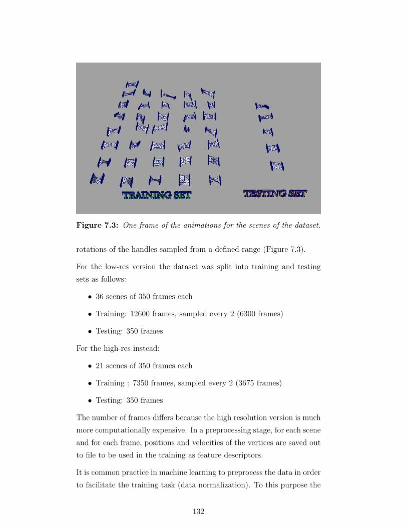
Figure 7.3: One frame of the animations for the scenes of the dataset.
rotations of the handles sampled from a defined range (Figure 7.3).
For the low-res version the dataset was split into training and testing
sets as follows:
• 36 scenes of 350 frames each
• Training: 12600 frames, sampled every 2 (6300 frames)
• Testing: 350 frames
For the high-res instead:
• 21 scenes of 350 frames each
• Training : 7350 frames, sampled every 2 (3675 frames)
• Testing: 350 frames
The number of frames differs because the high resolution version is much
more computationally expensive. In a preprocessing stage, for each scene
and for each frame, positions and velocities of the vertices are saved out
to file to be used in the training as feature descriptors.
It is common practice in machine learning to preprocess the data in order
to facilitate the training task (data normalization). To this purpose the
132

global mean and standard deviation on the six x,y,z coordinates of posi-
tion and velocity were calculated from all the samples of the training set,
then from each sample the mean was subtracted and the result divided
by the standard deviation. However for this specific problem the data
normalization did not improve the results therefore the dataset was left
as it is.
7.4 Architecture
The network architecture consists of 3 Convolutional layers (CL) followed
by a Fully Connected layer (FCL) used to reshape the output dimension.
The number of filters (output channels) are 64, 128 and 128 for the first,
second and third CLs respectively and 3 for the FCL (Figure 7.4).
Each CL uses Rectified Linear Units (ReLU) as activation functions.
Max pooling was not implemented because the meshes are not very high
resolution and also because it would imply using a decimation algorithm
between the layers.
The input of the network is a tensor data structure (multi-dimensional
array) of dimension [ number of vertices, 6 ], obtained as the result
of the stacking of two matrices of dimension [ number of vertices, 3 ]
representing the x,y,z components of positions and velocities. In the
case of the Recurrent Neural Network (RNN) implementation, the input
includes the time dimension and is a tensor of dimension [ sequence
length, number of vertices, 6 ]. The first 3 channels are the positions
and the ones from 4 to 6 are the velocities (x,y,z components). Given
the input at frame t, the output produced by the network is a tensor of
dimension [ number of vertices, 3 ] representing the predicted velocities
of the nodes at frame t+ 1 which are used to compute the new predicted
positions.
133
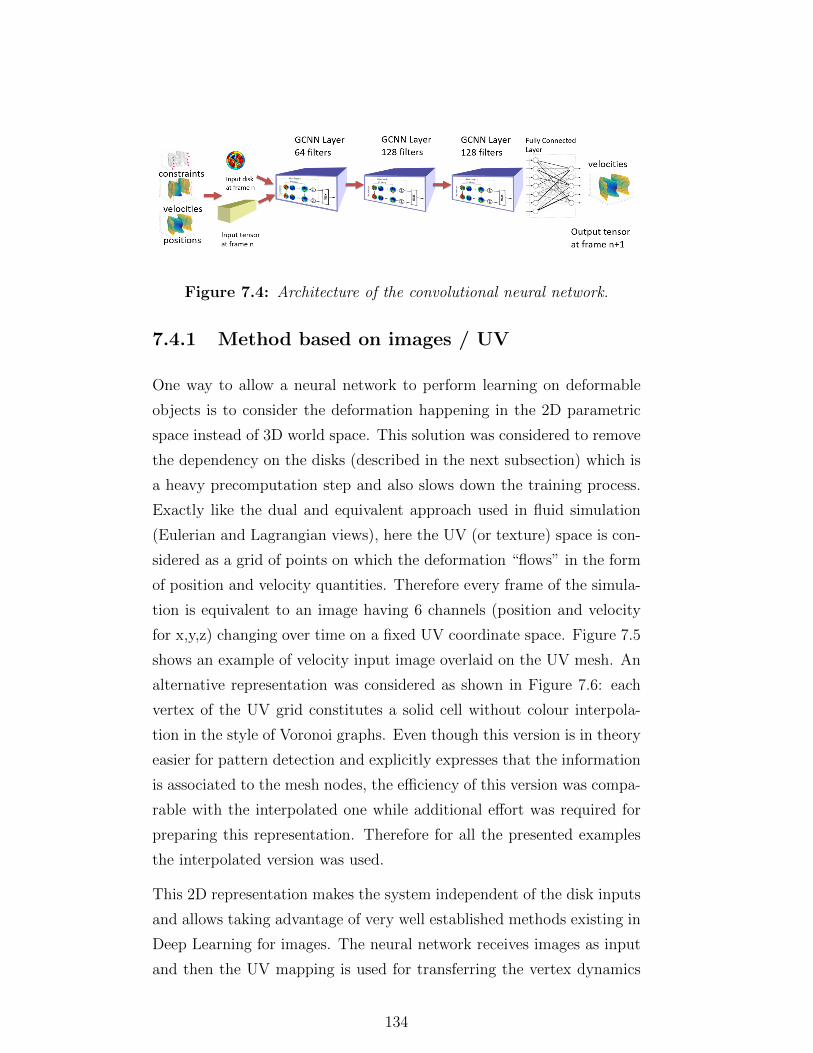
Figure 7.4: Architecture of the convolutional neural network.
7.4.1 Method based on images / UV
One way to allow a neural network to perform learning on deformable
objects is to consider the deformation happening in the 2D parametric
space instead of 3D world space. This solution was considered to remove
the dependency on the disks (described in the next subsection) which is
a heavy precomputation step and also slows down the training process.
Exactly like the dual and equivalent approach used in fluid simulation
(Eulerian and Lagrangian views), here the UV (or texture) space is con-
sidered as a grid of points on which the deformation “flows” in the form
of position and velocity quantities. Therefore every frame of the simula-
tion is equivalent to an image having 6 channels (position and velocity
for x,y,z) changing over time on a fixed UV coordinate space. Figure 7.5
shows an example of velocity input image overlaid on the UV mesh. An
alternative representation was considered as shown in Figure 7.6: each
vertex of the UV grid constitutes a solid cell without colour interpola-
tion in the style of Voronoi graphs. Even though this version is in theory
easier for pattern detection and explicitly expresses that the information
is associated to the mesh nodes, the efficiency of this version was compa-
rable with the interpolated one while additional effort was required for
preparing this representation. Therefore for all the presented examples
the interpolated version was used.
This 2D representation makes the system independent of the disk inputs
and allows taking advantage of very well established methods existing in
Deep Learning for images. The neural network receives images as input
and then the UV mapping is used for transferring the vertex dynamics
134
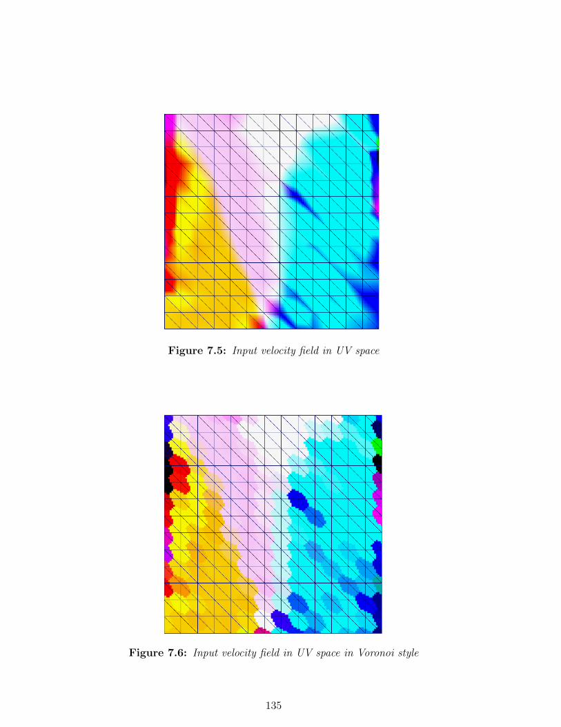
Figure 7.5: Input velocity field in UV space
Figure 7.6: Input velocity field in UV space in Voronoi style
135

data from 2D image space to 3D world space coordinates of the vertices
of the mesh. UVs can be assumed to be always present for an asset
in a Visual Effects production and can be generated semi-automatically
by modelling artists. This idea was tested and its results will be dis-
cussed in the following sections. The advantages over the version with
disks are that it offers rapid prototyping, allows faster training times and
resolution is more controllable.
7.4.2 Geodesic Convolution
The method described in the previous subsection makes use of standard
convolution layers. In order to operate directly on geometries defined in
3D world space, this work adopts a custom version of convolution lay-
ers specialized for meshes, introduced in Masci et al. (2015a). Given a
vector or scalar field defined on the vertices of the mesh, a geodesic disk
(patch) is defined per-vertex as a set of spatial kernel weights in geodesic
polar coordinates, by dividing the local neighbourhood into discrete bins.
Geodesic distances are the real distances from point to point on a mesh
for curved surfaces, as opposed to Euclidean distances which are just
the magnitude of the vector connecting two points. This disk, when
applied to the input field, extracts a local descriptor of it at a radius
distance (patch operator) in the form of a sparse matrix. A layer that
performs this kind of special convolution is called the Geodesic Convo-
lution Neural Network layer (GCNN). The disks, because are defined by
construction using geodesic distances, must be recomputed every time
the mesh deforms. As will be shown, this is one of the main limitations
of the method. In order to take advantage of the temporal coherence
of the inputs, the network is equipped with a skip connection from the
input to the output velocities: the input is summed to the predicted
values so that it already gives a good initial approximation instead of
being random, making the network learn de facto a velocity residual.
136
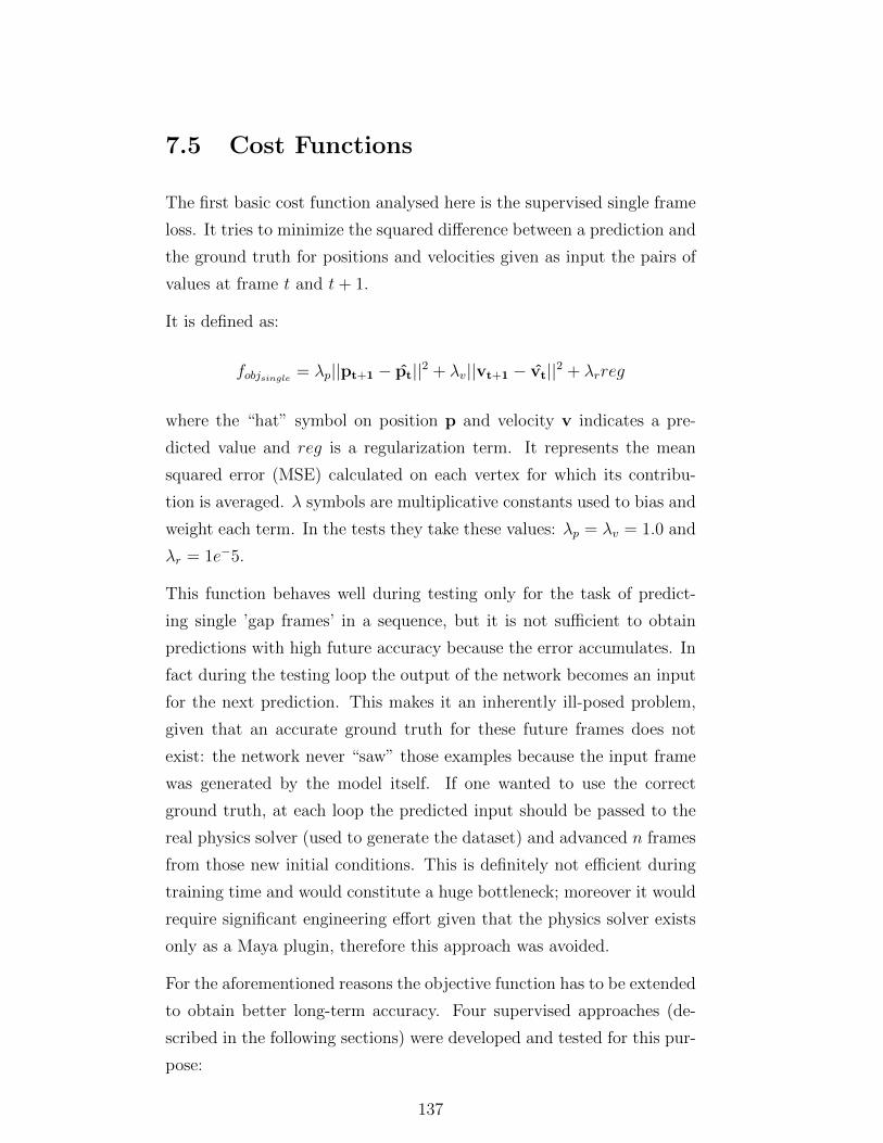
7.5 Cost Functions
The first basic cost function analysed here is the supervised single frame
loss. It tries to minimize the squared difference between a prediction and
the ground truth for positions and velocities given as input the pairs of
values at frame t and t+ 1.
It is defined as:
fobjsingle= λp||pt+1 − pt||2 + λv||vt+1 − vt||2 + λrreg
where the “hat” symbol on position p and velocity v indicates a pre-
dicted value and reg is a regularization term. It represents the mean
squared error (MSE) calculated on each vertex for which its contribu-
tion is averaged. λ symbols are multiplicative constants used to bias and
weight each term. In the tests they take these values: λp = λv = 1.0 and
λr = 1e−5.
This function behaves well during testing only for the task of predict-
ing single ’gap frames’ in a sequence, but it is not sufficient to obtain
predictions with high future accuracy because the error accumulates. In
fact during the testing loop the output of the network becomes an input
for the next prediction. This makes it an inherently ill-posed problem,
given that an accurate ground truth for these future frames does not
exist: the network never “saw” those examples because the input frame
was generated by the model itself. If one wanted to use the correct
ground truth, at each loop the predicted input should be passed to the
real physics solver (used to generate the dataset) and advanced n frames
from those new initial conditions. This is definitely not efficient during
training time and would constitute a huge bottleneck; moreover it would
require significant engineering effort given that the physics solver exists
only as a Maya plugin, therefore this approach was avoided.
For the aforementioned reasons the objective function has to be extended
to obtain better long-term accuracy. Four supervised approaches (de-
scribed in the following sections) were developed and tested for this pur-
pose:
137
• Future frames data augmentation
• Future frames partial derivatives accumulation
• Recurrent Neural Network
• SpatioTemporal convolution (for images version only)
All these objectives share the same limitations, as will be discussed in
the following sections.
7.5.1 Constraints
Constraints, intended as imposed boundary conditions by the user on
positions and velocities, play a very important role both in the simu-
lation and learning phase. Initially they were modelled as zero-length
spring energy potentials (see Chapter 4) so the system would penalize
the squared distance between the predicted and ground truth positions
if greater than zero. The problem with this approach for positional hard
constraints is that because it is an extra energy potential term (defined
in Section 4.3.4.1) added to the basic cost function’s objective, there
is the possibility that it will not be fully minimized. This means that
the network could not completely learn that some vertices should fol-
low the constraining objects. Therefore it was decided to not model the
constraints and instead pass the positions and velocities of the pinned
vertices in the input tensor.
In practice at preprocess stage all constrained vertices at time t are
overridden with the values of the ones of the ground truth at t + 1. In
the same way, at testing time, the predictions for the pinned vertices
are overwritten to follow the constraining objects. The ultimate decision
was to compute the objective function mask at training time only for the
unconstrained vertices. This allowed not only implementing constraints,
but also to simplify computations.
138
7.5.2 Future frames data augmentation
In the future frames approach a form of data augmentation is performed,
meaning that the dataset was extended procedurally at training time.
For each sample frame, during training the network is stepped forward
in the future 5 times and the predicted result is added to the training
samples using as ground truth the existing value of the sequence. If n
is the length of the sequence (350 in this work), then new samples are
added up to the frame n-5 of the sequence because the future frames after
that do not exist. In this approach the cost function stays the same as
for the single frame, just the dataset is extended on-the-fly at training
time.
7.5.3 Future frames partial derivatives accumula-
tion
In Tompson et al. (2016) the accumulation of future frames partial
derivatives is used to minimize the long term divergence of the veloc-
ity field. A similar technique is used in the approach described in this
section. In the same way as described in the previous subsection, at
each call of the training function for a sample, the network is stepped
forward 5 times, but the difference with the previous approach is that
the history in the forms of a computational graph of this future frame
is kept. This means that it is possible to do backpropagation through
time by first computing the partial derivatives (gradients) of the future
frame loss function and then accumulating (summing) them to the ones
of the current frame sample (see Tompson et al. (2016)). In practice this
is equivalent to minimizing in parallel the error that the network would
make in the future if outputting the current single frame prediction. The
gradients are necessary for the optimization algorithm to minimize the
objective via Stochastic Gradient Descent. In this work the adopted
descent algorithm is Adam (Kingma & Ba 2014).
139

7.5.4 RNN
A Recurrent Neural Network is able to keep a memory of what it has
“seen” in a sequence for a specified temporal window size. This allows it
to learn better patterns and features that evolve in time, making it par-
ticularly suitable for instance in Natural Language Processing and words
prediction in a sentence. For this reason, considering that a physics sim-
ulation is exactly a temporally coherent sequence of frames governed by
a law, it seems very appropriate to try this approach. While in the archi-
tectures presented before the input was a single pair of frames (t, t+ 1),
here the input is constituted by sequences of pairs of contiguous frames.
For example if the window size is 10 frames, the input is two sequences
10 samples long. An RNN can be thought of as a loop (recurrence) in
which at each step a new input of the sequence gets in and the output
feeds back into the network itself as a new hidden state (the equivalent
of a deep layer), in this way carrying along a memory. In this case the
layers are convolutional (GCNN) and the objective function is equivalent
to the previous ones.
To combat the long-term error accumulation all these strategies have
to use as inputs new samples generated on-the-fly at the previous time
step which means that new disks have to be recomputed. The reason is
that the new predicted frame geometry could be very different from the
existing ground truth of the dataset at that time. Therefore there is an
inherent error made when, instead of recomputing the disks, the existing
ones of the scene are used. But recomputing these disks n times (in this
case 5 steps in the future) for all the samples is computationally very
expensive, mainly because of the costly geodesic distances recalculation.
An alternative would be to use Euclidean distances, but for heavily de-
formed meshes this would introduce approximations that are too big and
consequently errors. For the exact method used to compute the geodesic
disks refer to Masci et al. (2015a).
140
7.5.5 Unsupervised Loss Function
By observing that a neural network is essentially a structured complex
optimizer and that the integration of the equations of motion can be seen
as an energy minimization, it seems logic trying to let the network learn
in a completely unsupervised manner. The objective function is defined
as:
fobjunsup = λdEdeform + λrreg (7.1)
with
Edeform =1
2h2‖M
12 (pn+1 − pn − hvn − h2M−1fext)‖2F +
∑i
Wi(pn+1)
which indicates the compromise that the optimization algorithm should
make between two terms. The first term expresses the momentum poten-
tial, that is the state the object will reach in a timestep if no internal or
external forces were acting on it. The second one is the elastic potential
energy (derivation of this formula is given in Bouaziz et al. (2014). This
formula, as mentioned in Chapter 2, follows by mathematically proving a
problem equivalence which results in what is called Variational Implicit
Euler in the literature. The goal is to find through a powerful regressor
(such as a deep neural network) the best configuration of vertex positions
such that the cost is minimized.
7.5.6 SpatioTemporal Convolution
In case the deformation happens in parametric space and the data is
packed into images as discussed in 7.4.1, the time component in the
learning process can be introduced by tweaking the input such that mul-
tiple frames are sent in order at the same time. This consists in stacking
position and velocity frames along the time component so that the con-
volution becomes spatio-temporal and is performed in three dimensions
with a 3D filter instead of just two. Assael et al. (2016) use this data
141
packing for video frames. The input data therefore becomes a tensor
of dimensions [ width, height, 3 * stack size]. The size of the stack, or
temporal window, is a parameter that can be chosen prior to training.
7.6 Training and Testing Process
The training process consists of the adjustment of the network weights
(filters) via backpropagation, using the gradients of the cost function for
each sample. The network is trained for a specified number of epochs;
an epoch consists in a loop in which all the samples are shown once to
the network. As is standard practice when dealing with neural network
training, the learning rate that is initialized at 0.001 is multiplied by
a factor of 0.8 every 10 epochs of no progress (i.e. no decrease of the
cost function), otherwise when there is progress the weights are saved
out to be used at testing time as the best result. Another regulariza-
tion technique adopted here is called dropout, which consists in setting
to zero the activation functions of some stochastically determined units
(neurons) of the network, a randomization that in practice is extremely
effective.
To improve generalization, the samples are never sent in the same order
during training, but randomly shuffled at each epoch. Moreover train-
ing is in general improved by using minibatches, consisting of groups of
samples minimized in the same backpropagation step: in this work the
batches are intended as groups of disk images on which to perform a
standard convolution and therefore are numberofvertices in size.
Gradient clipping was also used to prevent the phenomenon of gradients
explosion which could arise given the complex dataset.
As far as the testing phase is concerned, the important thing to notice
about dropout is that it must be disabled for the output to be determin-
istic. As mentioned earlier, at testing time disks are recomputed: even
if this contradicts with the purpose of creating a fast alternative to a
solver, it was the only way to test the validity of the technique.
142

Figure 7.7: Training (blue) and testing (red) curves for low res losswith future samples.
143
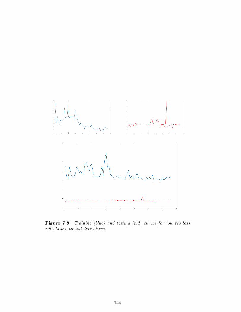
Figure 7.8: Training (blue) and testing (red) curves for low res losswith future partial derivatives.
144

Figure 7.9: Training (blue) and testing (red) curves for low res losswith RNN.
145
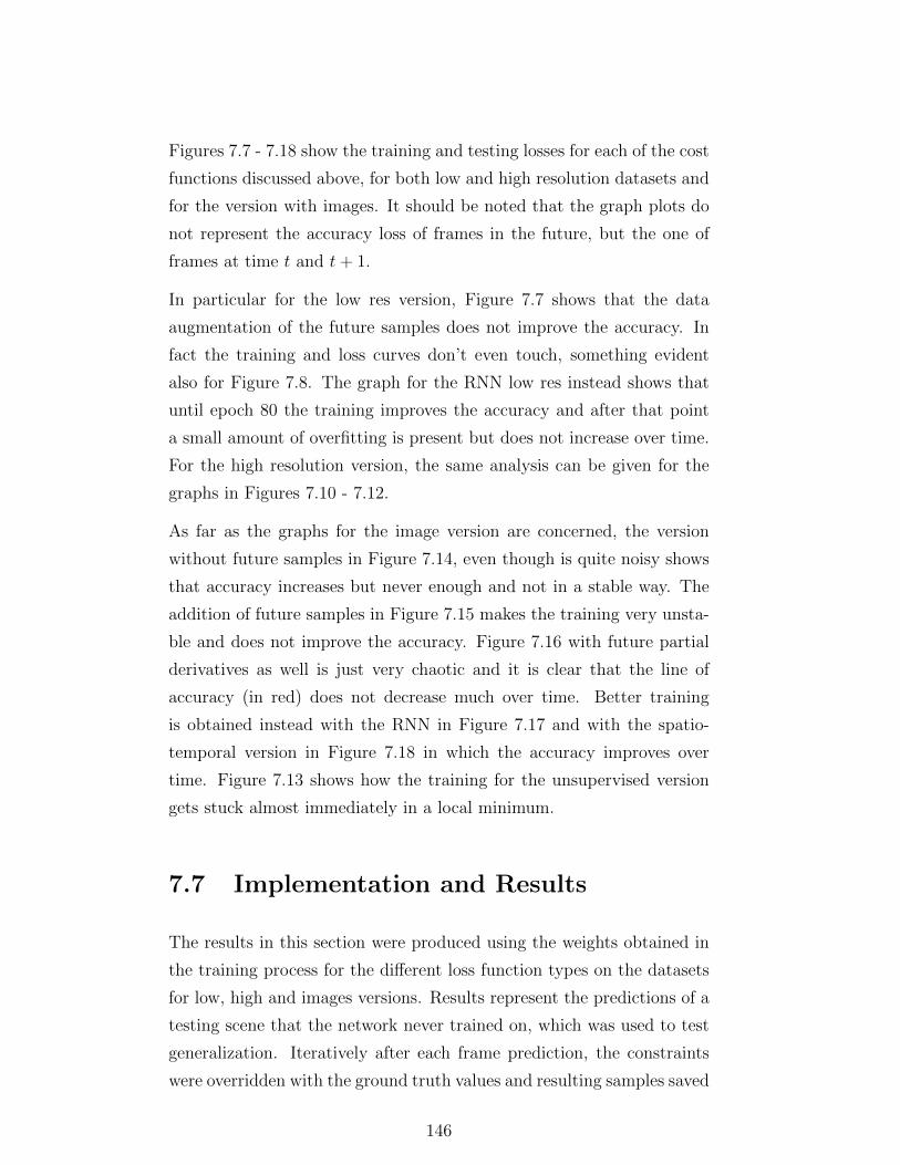
Figures 7.7 - 7.18 show the training and testing losses for each of the cost
functions discussed above, for both low and high resolution datasets and
for the version with images. It should be noted that the graph plots do
not represent the accuracy loss of frames in the future, but the one of
frames at time t and t+ 1.
In particular for the low res version, Figure 7.7 shows that the data
augmentation of the future samples does not improve the accuracy. In
fact the training and loss curves don’t even touch, something evident
also for Figure 7.8. The graph for the RNN low res instead shows that
until epoch 80 the training improves the accuracy and after that point
a small amount of overfitting is present but does not increase over time.
For the high resolution version, the same analysis can be given for the
graphs in Figures 7.10 - 7.12.
As far as the graphs for the image version are concerned, the version
without future samples in Figure 7.14, even though is quite noisy shows
that accuracy increases but never enough and not in a stable way. The
addition of future samples in Figure 7.15 makes the training very unsta-
ble and does not improve the accuracy. Figure 7.16 with future partial
derivatives as well is just very chaotic and it is clear that the line of
accuracy (in red) does not decrease much over time. Better training
is obtained instead with the RNN in Figure 7.17 and with the spatio-
temporal version in Figure 7.18 in which the accuracy improves over
time. Figure 7.13 shows how the training for the unsupervised version
gets stuck almost immediately in a local minimum.
7.7 Implementation and Results
The results in this section were produced using the weights obtained in
the training process for the different loss function types on the datasets
for low, high and images versions. Results represent the predictions of a
testing scene that the network never trained on, which was used to test
generalization. Iteratively after each frame prediction, the constraints
were overridden with the ground truth values and resulting samples saved
146

Figure 7.10: Training (blue) and testing (red) curves for high res losswith future samples.
147

Figure 7.11: Training (blue) and testing (red) curves for high res losswith future partial derivatives.
148

Figure 7.12: Training (blue) and testing (red) curves for high res losswith RNN.
Figure 7.13: Training (blue) and testing (red) curves for high res losswith unsupervised loss function.
149
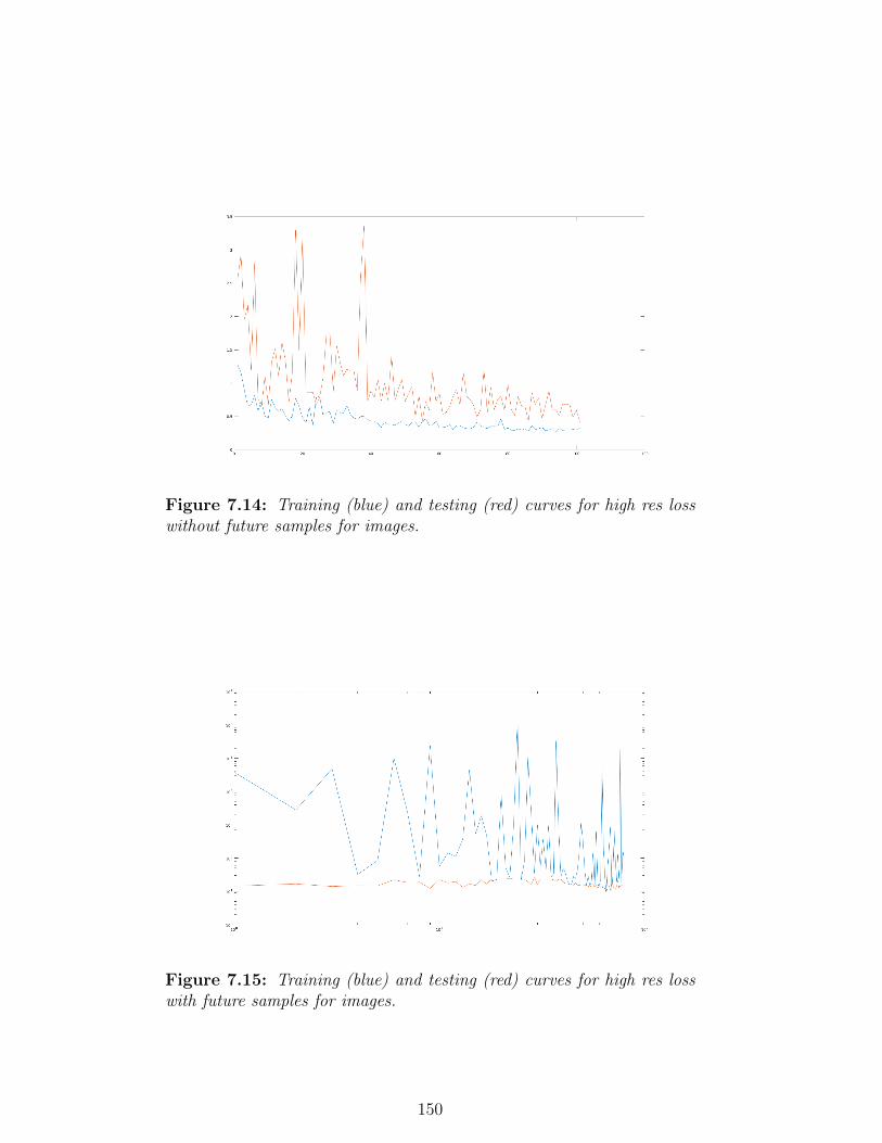
Figure 7.14: Training (blue) and testing (red) curves for high res losswithout future samples for images.
Figure 7.15: Training (blue) and testing (red) curves for high res losswith future samples for images.
150

Figure 7.16: Training (blue) and testing (red) curves for high res losswith future partial derivatives.
Figure 7.17: Training (blue) and testing (red) curves for high res losswith RNN for images.
151

Figure 7.18: Training (blue) and testing (red) curves for high res losswith spatio-temporal convolution for images.
to disk to become new input for the subsequent loop.
Figures of the results (see Figures 7.19 - 7.30) seem to indicate that the
future frames inclusion in the training is crucial for a good outcome for
the predicted simulation. Moreover they suggest that without accurate
disks the network is learning a wrong projection, demonstrated by the
fact that for all the cases, after about 15 frames the error just keeps ac-
cumulating until distorting heavily the mesh. This seems unfortunately
the price to pay for the use of the precomputed disks during training,
disks that are associated to a mesh that differs from the predicted one.
Another reason why the network is not learning a good projection could
be that the adopted dataset is still too small and not diverse enough.
In terms of dynamics prediction quality, the RNN gives the most promis-
ing results (Figures 7.19 and 7.22) confirming the supposition that a tem-
poral sequence in the input helps the network infer time-varying prop-
erties and patterns better. However, because the RNN does not adopt
any long-term error reduction strategy, it still produces very distorted
meshes.
The unsupervised loss function does not produce the expected results.
A test was performed in which the minimization of one frame done by
the network is compared with the result obtained by substituting in
152

Figure 7.19: Low res pairs of results (predicted, ground truth) for sam-pled frames in range 100-160 of the testing scene for RNN.
Equation 7.1 the ground truth frame t+ 1: the network converges to the
same result, but when trying to minimize all the frames of the scenes it
simply gets stuck (Figures 7.13 and 7.25). One of the possible reasons
is that the minimization should lead to different positive scalar values
of the loss function for each frame because the elastic energy depends
on the shape and the momentum potential from the inertia at that time
frame and is almost never equal to zero.
As far as the version with images is concerned, a qualitative and vi-
sual analysis of the results shows that all tests except the RNN do not
produce satisfying behaviour: the dynamics are plausible only for the
153

Figure 7.20: Low res pairs of results (predicted, ground truth) for sam-pled frames in range 100-160 of the testing scene for partial derivatives.
154

Figure 7.21: Low res pairs of results (predicted, ground truth) for sam-pled frames in range 100-160 of the testing scene for future samples.
155
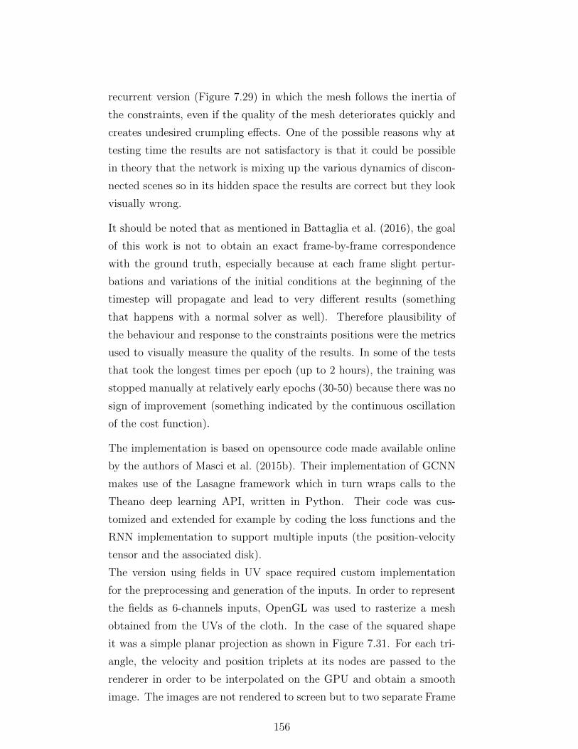
recurrent version (Figure 7.29) in which the mesh follows the inertia of
the constraints, even if the quality of the mesh deteriorates quickly and
creates undesired crumpling effects. One of the possible reasons why at
testing time the results are not satisfactory is that it could be possible
in theory that the network is mixing up the various dynamics of discon-
nected scenes so in its hidden space the results are correct but they look
visually wrong.
It should be noted that as mentioned in Battaglia et al. (2016), the goal
of this work is not to obtain an exact frame-by-frame correspondence
with the ground truth, especially because at each frame slight pertur-
bations and variations of the initial conditions at the beginning of the
timestep will propagate and lead to very different results (something
that happens with a normal solver as well). Therefore plausibility of
the behaviour and response to the constraints positions were the metrics
used to visually measure the quality of the results. In some of the tests
that took the longest times per epoch (up to 2 hours), the training was
stopped manually at relatively early epochs (30-50) because there was no
sign of improvement (something indicated by the continuous oscillation
of the cost function).
The implementation is based on opensource code made available online
by the authors of Masci et al. (2015b). Their implementation of GCNN
makes use of the Lasagne framework which in turn wraps calls to the
Theano deep learning API, written in Python. Their code was cus-
tomized and extended for example by coding the loss functions and the
RNN implementation to support multiple inputs (the position-velocity
tensor and the associated disk).
The version using fields in UV space required custom implementation
for the preprocessing and generation of the inputs. In order to represent
the fields as 6-channels inputs, OpenGL was used to rasterize a mesh
obtained from the UVs of the cloth. In the case of the squared shape
it was a simple planar projection as shown in Figure 7.31. For each tri-
angle, the velocity and position triplets at its nodes are passed to the
renderer in order to be interpolated on the GPU and obtain a smooth
image. The images are not rendered to screen but to two separate Frame
156
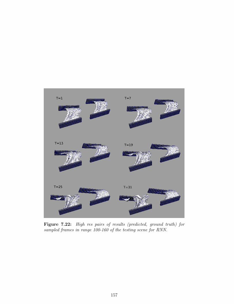
Figure 7.22: High res pairs of results (predicted, ground truth) forsampled frames in range 100-160 of the testing scene for RNN.
157
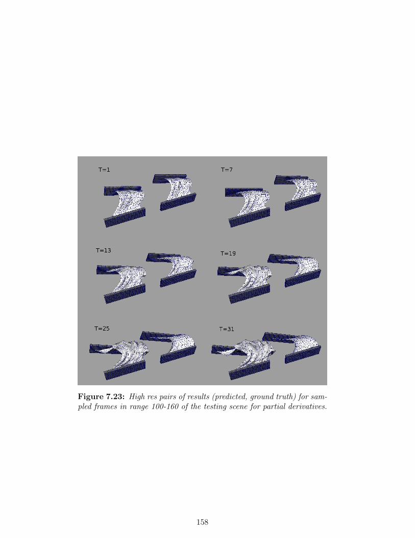
Figure 7.23: High res pairs of results (predicted, ground truth) for sam-pled frames in range 100-160 of the testing scene for partial derivatives.
158

Figure 7.24: High res pairs of results (predicted, ground truth) forsampled frames in range 100-160 of the testing scene for future samples.
159
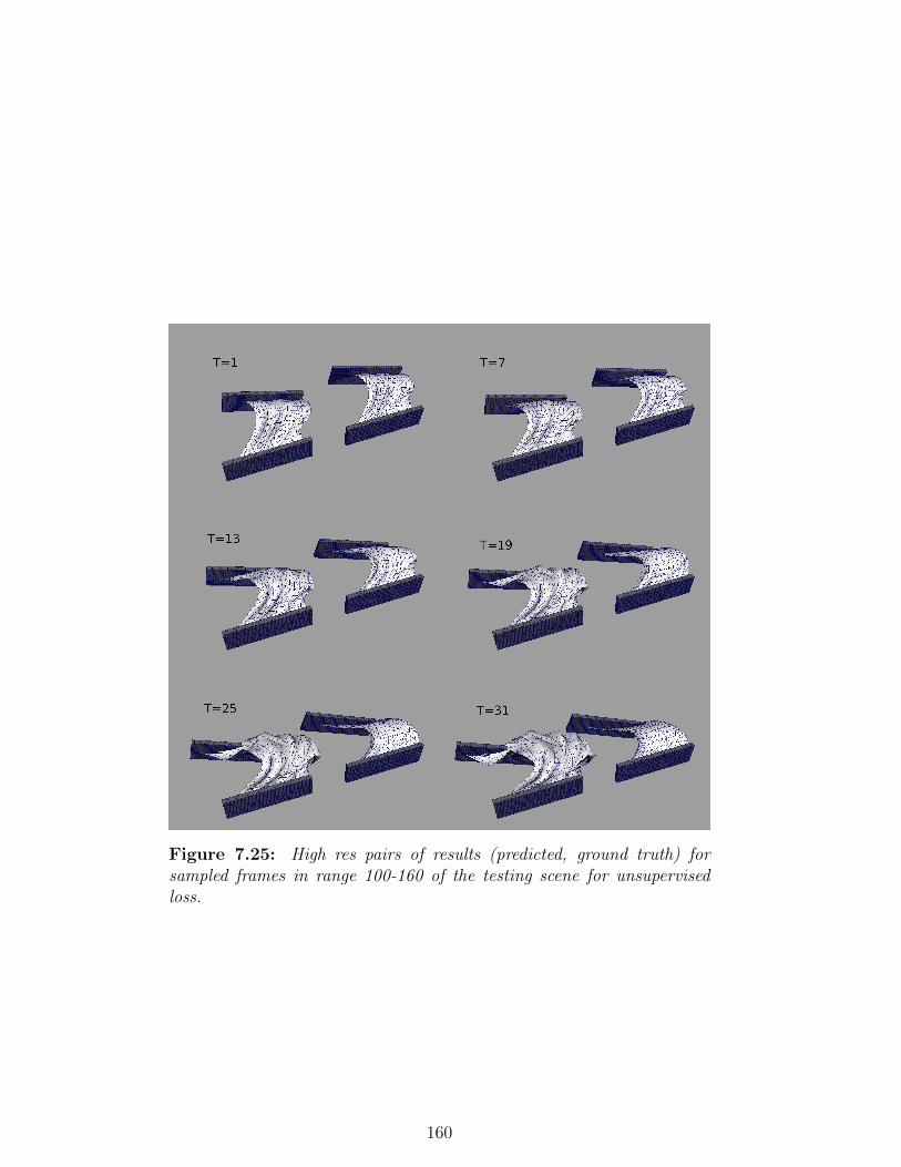
Figure 7.25: High res pairs of results (predicted, ground truth) forsampled frames in range 100-160 of the testing scene for unsupervisedloss.
160

Figure 7.26: High res pairs of results (predicted, ground truth) for sam-pled frames in range 100-160 of the testing scene without future samples(images).
161
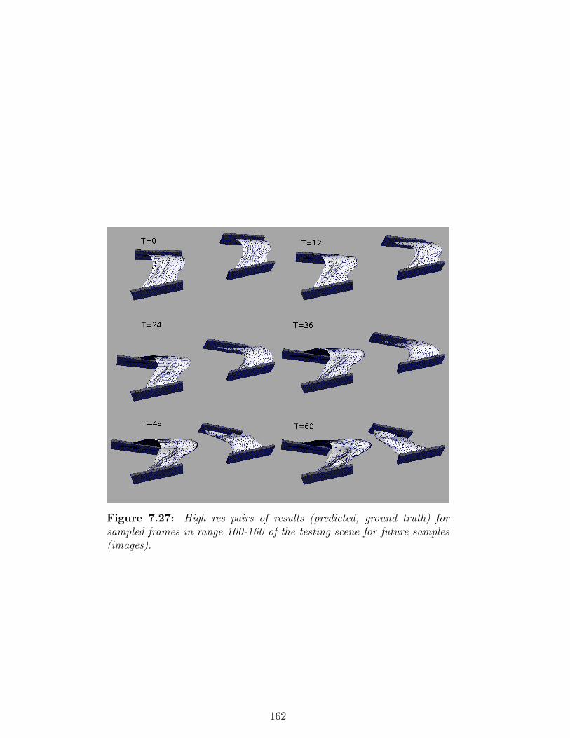
Figure 7.27: High res pairs of results (predicted, ground truth) forsampled frames in range 100-160 of the testing scene for future samples(images).
162

Figure 7.28: High res pairs of results (predicted, ground truth) for sam-pled frames in range 100-160 of the testing scene for partial derivatives(images).
163
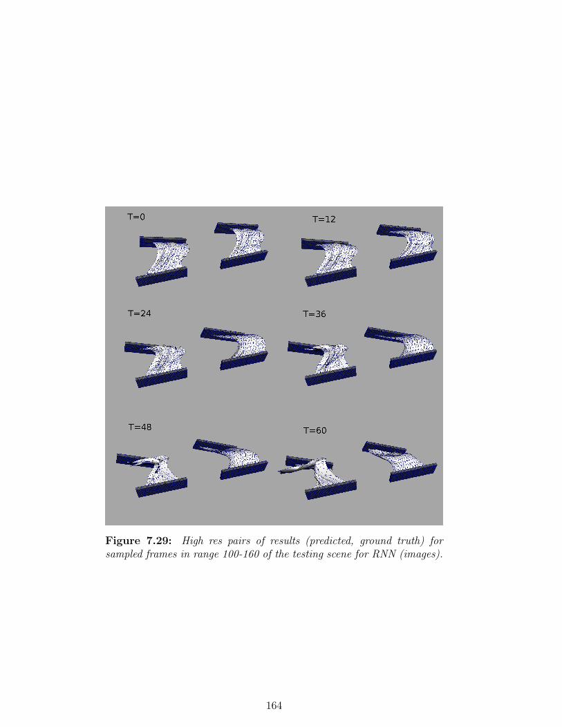
Figure 7.29: High res pairs of results (predicted, ground truth) forsampled frames in range 100-160 of the testing scene for RNN (images).
164
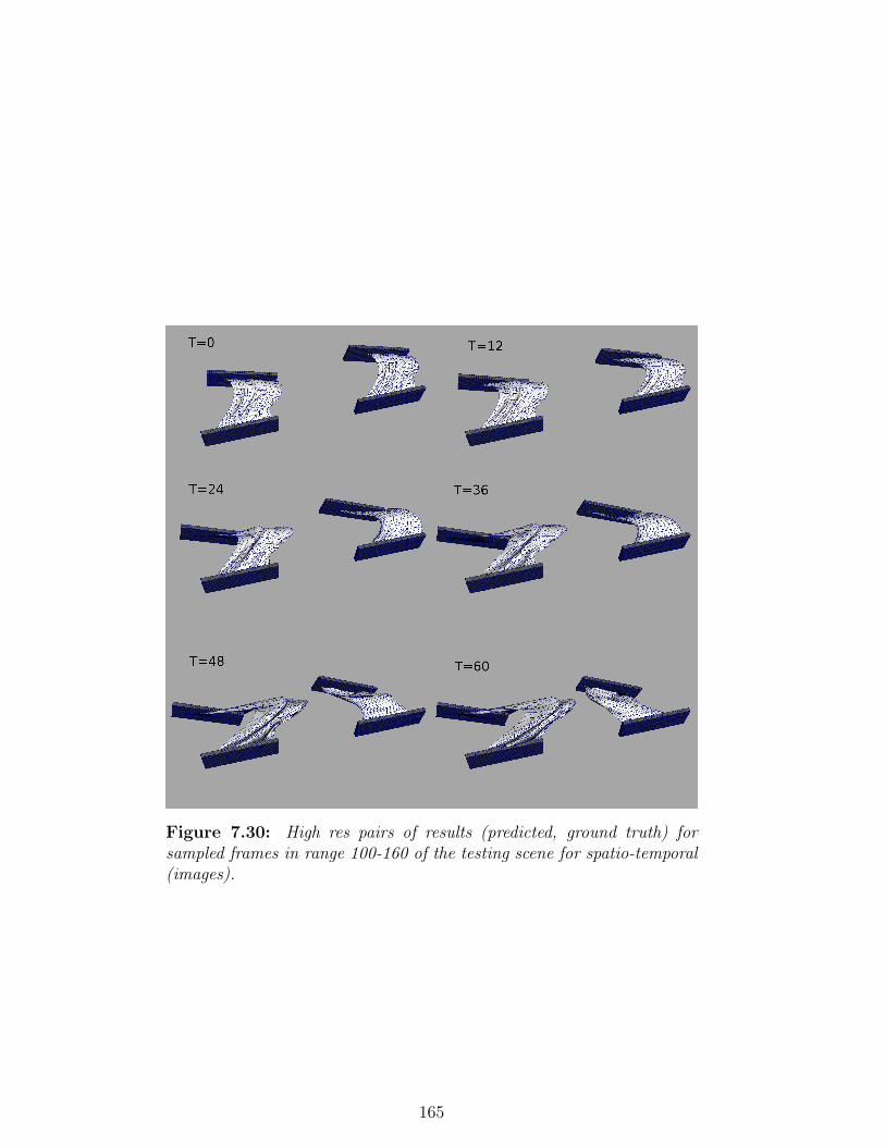
Figure 7.30: High res pairs of results (predicted, ground truth) forsampled frames in range 100-160 of the testing scene for spatio-temporal(images).
165

Figure 7.31: UVs. Nodes corresponding to the rendered 2D mesh forfield values interpolation in green.
Buffer Objects as signed floats, after disabling clamping. During train-
ing and prediction, the renderer is called to override the triangles that
contain constrained vertices because the predicted and constrained node
values need to be re-interpolated. Another possible explanation of the
problems appearing in the results is the relatively low resolution of the
images. In the implementation it was 128x128 pixels.
Training was done on a NVIDIA Titan Xp and on a laptop NVIDIA
GTX 780M.
The work presented in this chapter on machine learning concludes the
part on the projects completed during the EngD in the hosting com-
166

panies. The next and last part of this thesis draws the conclusions,
discusses limitations and proposes future work for all the projects previ-
ously described.
167

Part III
Conclusions and Future Work
168

Chapter 8
Conclusions and Future Work
This thesis has discussed possible new directions and approaches that
can be taken towards the production of realistic deformations for digital
characters in a modern movie production pipeline. This chapter draws
both specific (i.e. by project) and general conclusions based on the work
completed, together with avenues for future work.
8.1 Conclusions
Active research on methods for the deformation of musculo-skeletal sys-
tems is a vital part of modern VFX. On the one hand the needed
plausible and visually realistic results can be obtained with stable, ac-
curate and computationally efficient deformation algorithms. On the
other hand these technical improvements must be inserted in an artist-
driven pipeline in which many software programs and technologies co-
exist. Artists often need to abstract from underlying technicalities and
need interactive tools in order to express their creative intent in an envi-
ronment characterized by continuous iterations. This work was therefore
motivated by the need to improve both these two aspects related to the
problem of obtaining visually convincing animated characters, bringing
contributions to a specific part of the movie creation pipeline.
In this work several techniques covering different aspects of muscle defor-
169

mation and, in general, physically-based animation have been presented:
• The creation of a custom simulation framework using FEM built
on top of the VEGA library to help the company to test a new
physically-based approach to character deformation. Formulas were
derived to implement muscle activations for a constitutive material
enriched with fibres. Constraints and collisions were also added to
the framework contributing to the creation of a usable prototype.
• The creation of a novel method consisting of the interactive physics-
based design of anatomical muscle geometries ready to be simu-
lated. This method responds to the need for faster systems to
model volumetric anatomically-plausible shapes.
• The development of a tool and a workflow, based on the simulation
framework previously created, focused on the interactive placement
of muscle geometries on a skeletal bones rig which takes into con-
sideration collisions.
• A procedural method for skinning that uses implicitly-defined scalar
fields to create wrinkle effects.
• The investigation of the application of Deep Learning to the sim-
ulation of deformable objects with the aim of improving the speed
of a standard solver.
Except for the last pilot study on deep learning, the results obtained in
each of the projects were mainly successful and even though they were
not directly used in production, the tools and software developed are at
the working prototype stage. Considering that most of them are already
in the form of a Maya plugin, they can be deployed to the real pipeline
without significant difficulties.
The subsections below present conclusions for each of the projects con-
tained in this thesis, in order of appearance.
170

8.1.1 Muscle primitives modelling
The muscle primitives modelling described in Chapter 3 produced re-
sults that matched the initial goals of the project. Instead of sculpting
each muscle separately using anatomy references, the goal was to find an
alternative semi-automatic way to obtain plausible volumetric muscles
by taking advantage of the benefits of a simulated approach. The pro-
posed physics-based approach demonstrated to be a valid way to produce
volumetric models and their associated fibre field from a limited input
sketched directly on the surface of the character. The system was ap-
plied to the production-inspired use case of a muscular human arm and
obtained realistic output contractions.
Despite the promising results, the system has some limitations and space
for improvement. The areas at the borders of the patch are in fact still
quite sharp and could be made smoother by adding custom energy terms,
using greater resolution or turning the constrained vertices at the border
into soft constraints. Some produced muscles, because of the flatness
of the source patch, do not always fill all the available interior space
and leave gaps between them and the bones. One could increase the
pressure, use a softer material or run the inflation process for a longer
time to improve on these issues. In the examples the presence of a fat
layer between muscles and skin was discarded, considering the specific
3D model of a lean muscular body type examined. As an effect it was
easier to sketch patches on the visible skin and the resulting muscle
primitives are bigger than they should be. An offset based on a specified
3D texture could be applied per patch to take the fat into account (Saito
et al. (2015)).
An alternative to the manual sketch of the patches, provided that the
mesh contains texture mapping with UV coordinates, would be to use a
texture template containing a representation of the muscle anatomy; the
initial patches could be automatically generated based on segmentation
of RGB colour values which could be used to transfer them between
characters. This would also be an efficient way to bootstrap the patches
because even though for lean and muscular characters the details on the
171

skin are enough to distinguish most of the superficial muscles, the fat
layer often present in characters smooths out these details and hides the
underlying anatomy.
8.1.2 Muscle simulation framework
The muscle simulation framework described in chapter 4 produces very
convincing results which demonstrate that a modern character produc-
tion pipeline should include simulation to obtain visually plausible defor-
mations with dynamics. The goal of proposing to the hosting company
an evolution from the existing the semi-procedural system to one fully
based on physics was at least in part achieved, through the development
of a working prototype that showed detailed effects such as muscle and
bones sliding, active muscle contractions and colliding biological tissues.
The use case on which the framework was tested was the animation of
a human arm. Their generality means that the same methods are appli-
cable to CG animals or fantasy creatures having the same or a different
combination of anatomical layers.
In addition to the complexity needed to have a good anatomical model,
which can be mitigated but is still present, the limitations of the proposed
framework are represented by the speed of simulation especially in the
presence of many collision constraints and by the lack of an intuitive
user interface. Moreover, in the presence of very highly constrained and
compressed areas in contact (in a real character for example in the armpit
region), the stability of the solver could suffer if a very small timestep is
not used.
8.1.3 Placement of simulation-ready muscles
Chapter 5 presented a workflow aimed at helping the modelling of simulation-
ready muscles in a production environment for the Visual Effects indus-
try. It showed very promising results by proposing an integrated solution
to a practical problem that rigging artists face while creating complex
172

muscle systems. An artist in general spends a good amount of time plac-
ing complex organic shapes and then fixing their interpenetrations so
this system would be beneficial.
One of the limitations is that the system was developed as a proof-of-
concept prototype and is therefore yet to be fully tested before going into
the production pipeline to test its effective advantage over an already well
established workflow. The scalability to a full character was not tested;
however because already placed muscles are static and their contact is
computed fast, this is not likely to be a real problem. Finally it should
be noted that to use the system effectively an artist would need to invest
time on initial basic training because a physics-based approach is a new
modelling paradigm that needs to be learned and developed like any
other skill.
8.1.4 Procedural wrinkles
The technique presented in Chapter 6 to obtain wrinkles creates plausible
results even comparable with physically accurate stretch-based methods.
The initial goal of extending an existing procedural method by exploit-
ing its constitutive parts was achieved and its generalization properties
tested. The results show its potential for applications within a produc-
tion pipeline.
Despite its potential, the technique for procedural wrinkles has some
limitations. For example, being the output of the deformation time-
dependent, finding the right parameters could require various iterations,
something that makes it close in spirit to a simulation. Nevertheless,
the user can always tweak single frames without rerunning the whole
animation; in this case wrinkles will form following only the field at the
current frame. In addition, it should be noticed that the quality of the
fields tends to depend on the input shape, something that might limit
the technique to cylindrical limbs and prevent the application to, for
instance, face wrinkles generation.
173

8.1.5 Deep learning for deformable objects
The last project presented in this thesis in Chapter 7 did not fully meet
the initial goals and expectations, but nevertheless constituted a great
learning opportunity. In fact the objective was to obtain in a relatively
short time convincing predictions for a toy problem such as a cloth simu-
lation and at a later stage extend the system to muscle dynamics regres-
sion. Inspired by recent research, a variety of neural network architec-
tures and loss functions (supervised and unsupervised) were tested and
compared, but produced dynamic predictions with a medium-low level
of accuracy; this fact prevented its extension to muscles.
One of the main limitations of the work on Deep Learning for deformable
objects is that the system did not learn properly how to compensate for
future errors therefore the quality and length of the predictions is limited
to 20-30 frames and correct dynamics were not fully accomplished. More-
over, a simulation using a different mesh with different topology whould
require in principle a new training of the network. However, as noted
in Tompson et al. (2016), because the network is fully-convolutional the
size of the input domain could be changed at inference time while train-
ing on a single resolution. This property was not verified in this work.
Because of the bottleneck constituted by the disks, a comparison of exe-
cution times with a GPU physics solver was not done. This would have
required a porting of the existing CPU based solver used to generate the
dataset.
8.2 Future Work
The techniques proposed in this thesis constitute a small part of the
ideal framework that is necessary in a real production, therefore they
are not complete or in their final form. Below will be given directions
for improvement and future work for each of the projects in order of
appearance in this thesis.
For the muscle primitives modelling project, in addition to extending the
174

system to the full body and trying out methods of transferring patches
across characters, it would be an interesting future direction to test the
application of a plasto-elastic material model and adaptive meshes.
Regarding the actual simulation system of chapter 4, even though the
results are realistic and appreciated in the hosting company, a lot can
be done to improve the realism, the usability of the framework and the
efficiency. For example in the presented examples the coupled action
between muscles and skin was mostly ignored: not only the skin should
stretch and deform due to the underlying contracting muscles, but in
turn it should produce a containing effect back onto the muscles in the
form of an elastic forces response. To obtain this, the layers should be
simulated all at once and not separately cached. To add even more re-
alism, veins could be modelled from anatomy references as curves and
their geometry could be merged with the skin or used as a displacement
map. During simulation they could deform together with the skin layer
and their thickness could be animated based on the muscle activation
level and isometric contraction duration. In terms of artistic control, to
direct the physics simulation a technique such as the one described in
Martin et al. (2011) could be used, in which custom shapes are inserted
in the dynamics of the solver and work as force attractors interpolated
in strain space. This method seems to work very well, even though one
of the drawbacks is that if the artist creating the shapes is not accu-
rate enough, constraints such as volume preservation could be violated
and the system could not be aware of it. Another possibility would be
to inject custom shapes as new per-frame rest poses of the solver as in
Kozlov et al. (2017). Also, tools to allow artists to groom complex net-
works of fibres to control the muscle shape would be greatly beneficial.
One of the areas of research that would bring huge benefit to the indus-
try is the development of a unified solver with coupling that stably and
accurately supports deformable objects, hair, particles, cloth, and rigid
bodies simulation. In fact a digital character almost always contains
parts or accessories that can be modelled and simulated in one of those
ways.
As far as the muscle placement system is concerned, there are many ar-
175
eas of improvement on which to focus. First of all, it would be desirable
to adapt a constraint-based dynamics approach to avoid the problems
of stability of penalty forces when high stiffness makes the system ma-
trix poorly conditioned. To increase the user experience and make the
simulation more closely resemble the desired results, it would be also
beneficial to add an external skin mesh representing the superficial fas-
cia as a boundary condition surface on which both the sculpting tool and
the simulation can collide against. For the placement stage, it would be
useful to add a plastic deformation functionality directly integrated in
a fast solver as in Saito et al. (2015) , in which a decomposition of the
deformation gradient is used to grow the muscles. A seamless integration
of the modelling and placement plugins, now separated, would avoid a
context-switch problem that can absorb time from the creative process.
Moreover in terms of performance the code could be parallelized much
more (for example for the internal force computation) and a simplified
GPU version of the solver would boost the speed even more. Finally, be-
cause a FEM solver could be an too computationally expensive for this
problem, other solvers based on PBD or XPBD may be a better option
to consider.
For the Implicit Skinning project, as future work, the intention is to
integrate adaptive tessellation technology. Even though in a production
pipeline it is not common to have varying topology, the performance
would benefit by having more detail only where needed, with the option
to export displacement maps for rendering. It would also be useful to
investigate ways to make the convolution surfaces look less cylindrical
and more organic, not restricted only to circular profiles; for example
noise could be added, or segments with different radius could be layered.
Moreover, another interesting future direction inspired by Cao et al.
(2015) would be to combine the proceduralism of the method with a
trained approach in order to learn the space of input parameters for
a closer match to the physical appearance of acquired data. Finally, a
better falloff of the radius per curve would be desirable as wrinkles should
fade away the further they are from the joint.
In terms of the machine learning project in chapter 7, given the un-
176
derstanding of some of the reasons why the system is underperforming,
various avenues for future work can be taken. First of all there is clearly
a need to research improvements on the speed of disk computation, with
the aim of real-time performance. Progress in this direction is being made
in the work by Monti et al. (2016). The computation of the disks using
Euclidean distances was not tested to measure the actual performance
and accuracy, therefore it would be useful for comparison. Alternatively,
the on-the-fly recomputation of geodesic distances could be done only for
some random samples of the training set. Minibatches of frames should
also be used to improve the training, while at the moment the batches
have dimension the number of vertices, containing one image per vertex.
Max pooling is another technique used to improve generalization and
performance during training that would be appropriate to implement.
After each convolution the output dimension is halved multiple times
so the most significant features remain. However this downsampling
would be applied on the mesh topology by a decimation algorithm and
it is yet to be demonstrated if it would benefit the learning process. In
terms of improvements to the loss functions, extra terms considered for
future work would be the volume (area) preservation for the predicted
triangles using the determinant-based formulation found for example in
Ichim et al. (2017) and a term to preserve an amount of smoothness of
the mesh to avoid heavy distortions. Finally, research is needed to extend
the convolution to support tetrahedral volumetric objects via spherical
coordinates disks so that the learning method can be applied to geome-
tries representing muscles and fat.
As a final closing note, it should be always kept in mind that technologies
and consequently workflows evolve fast and this is true especially for
Visual Effects, considering the recent and current industry trends. In
fact if I could start my EngD again I would focus predominantly on
real-time and interactive methods rather than using FEM just because
it is accurate. The Visual Effects industry is going through a major
177

revolution in which game engines are more and more a fundamental part
of movie production stages such as pre-visualization, camera motion,
interactive design of environments, look development and lighting. The
coming wave of Virtual and Augmented Reality (VR/AR) also requires
that realistic character deformation must happen in real time. The idea
of contributing to the creation of illusive but magical, emotional and
immersive experiences constitutes the beauty of doing research in this
exciting field.
178
References
D. Ali-Hamadi, et al. (2013). ‘Anatomy Transfer’. ACM Trans. Graph.
32(6):188:1–188:8.
Andrej Karpathy (2017). ‘CS231n Convolutional Neural Networks for
Visual Recognition’. http://cs231n.github.io/.
D. Anguelov, et al. (2005). ‘SCAPE: Shape Completion and Animation
of People’. ACM Trans. Graph. 24(3):408–416.
Y. M. Assael, et al. (2016). ‘LipNet: Sentence-level Lipreading’. CoRR
abs/1611.01599.
D. Baraff & A. Witkin (1998). ‘Large steps in cloth simulation’. In
Proceedings of the 25th annual conference on Computer graphics and
interactive techniques, pp. 43–54. ACM.
J. Barbic & D. L. James (2005). ‘Real-Time Subspace Integration for
St. Venant-Kirchhoff Deformable Models’. In ACM SIGGRAPH 2005
Papers, SIGGRAPH ’05, pp. 982–990, New York, NY, USA. ACM.
J. Barbic, et al. (2012). ‘Interactive Editing of Deformable Simulations’.
ACM Trans. on Graphics (SIGGRAPH 2012) 31(4).
P. W. Battaglia, et al. (2016). ‘Interaction Networks for Learning about
Objects, Relations and Physics’. CoRR abs/1612.00222.
B. Bickel, et al. (2009). ‘Capture and Modeling of Non-linear Heteroge-
neous Soft Tissue’. In ACM SIGGRAPH 2009 Papers, SIGGRAPH
’09, pp. 89:1–89:9, New York, NY, USA. ACM.
S. Blemker & S. Delp (2005). ‘Three-Dimensional Representation of
179

Complex Muscle Architectures and Geometries’. Annals of Biomedical
Engineering 33(5):661–673.
S. S. Blemker, et al. (2005). ‘A 3D model of muscle reveals the causes
of nonuniform strains in the biceps brachii’. Journal of Biomechanics
38(4):657–665.
J. Bonet & R. D. Wood (1997). Nonlinear continuum mechanics for
finite element analysis. Cambridge university press.
S. Bouaziz, et al. (2014). ‘Projective Dynamics: Fusing Constraint Pro-
jections for Fast Simulation’. ACM Trans. Graph. 33(4):154:1–154:11.
R. Bridson, et al. (2003). ‘Simulation of clothing with folds and wrinkles’.
In Proceedings of the 2003 ACM SIGGRAPH/Eurographics symposium
on Computer animation, pp. 28–36. Eurographics Association.
M. M. Bronstein, et al. (2016). ‘Geometric deep learning: going beyond
Euclidean data’. CoRR abs/1611.08097.
C. Cao, et al. (2015). ‘Real-time High-fidelity Facial Performance Cap-
ture’. ACM Trans. Graph. 34(4):46:1–46:9.
CGCircuit (2016). ‘CGCircuit Tutorial, Skinning with nCloth’.
https://www.cgcircuit.com/tutorial/skinning-with-ncloth/.
Chaos Group (2015). ‘Introduction to deformable objects models and
muscle simulation - Fabio Turchet, MPC London, CG2 Talk Code’.
https://www.youtube.com/watch?v=i2s120TV-F0.
H. Choi & S. Blemker (2013). ‘Skeletal Muscle Fascicle Arrangements
Can Be Reconstructed Using a Laplacian Vector Field Simulation’.
PLoS ONE 8(10)(e77576).
K.-J. Choi & H.-S. Ko (2002). ‘Stable but Responsive Cloth’. ACM
Trans. Graph. 21(3):604–611.
S. Clutterbuck & J. Jacobs (2010). ‘A physically based approach to
virtual character deformation’. In ACM SIGGRAPH 2010: Talks.
O. Comas, et al. (2008). ‘Efficient Nonlinear FEM for Soft Tissue Mod-
elling and Its GPU Implementation within the Open Source Frame-
180
work SOFA’. In F. Bello & P. Edwards (eds.), Biomedical Simulation,
vol. 5104 of Lecture Notes in Computer Science, pp. 28–39. Springer
Berlin Heidelberg.
S. Comer, et al. (2015). ‘Under the Scalpel - ILM’s Digital Flesh Work-
flows’. In ACM SIGGRAPH 2015 Talks, SIGGRAPH ’15, pp. 10:1–
10:1, New York, NY, USA. ACM.
M. Cong, et al. (2015). ‘Fully Automatic Generation of Anatomical Face
Simulation Models’. In Proceedings of the 14th ACM SIGGRAPH /
Eurographics Symposium on Computer Animation, SCA ’15, pp. 175–
183, New York, NY, USA. ACM.
S. Delp, et al. (2007). ‘OpenSim: Open-Source Software to Create and
Analyze Dynamic Simulations of Movement’. Biomedical Engineering,
IEEE Transactions on 54(11):1940–1950.
Fabric Engine (2015). ‘Fabric Engine’. http://fabricengine.com/.
Y. Fan, et al. (2014). ‘Active Volumetric Musculoskeletal Systems’. ACM
Trans. Graph. 33(4):152:1–152:9.
C. Flynn & B. Mccormack (2009). ‘Simulating the wrinkling and aging
of skin with a multi-layer finite element model’ 43:442–8.
S. Fortier (2013). ‘Fortier, S.’. http://www.simonefortier.com/fascia-
stretching-therapy/.
J. Gain & D. Bechmann (2008). ‘A Survey of Spatial Deformation from
a User-centered Perspective’. ACM Trans. Graph. 27(4):107:1–107:21.
T. Geijtenbeek, et al. (2013). ‘Flexible Muscle-based Locomotion for
Bipedal Creatures’. ACM Trans. Graph. 32(6):206:1–206:11.
I. Goodfellow, et al. (2016). Deep Learning. MIT Press. http://www.
deeplearningbook.org.
E. Guerin, et al. (2017). ‘Interactive Example-based Terrain Author-
ing with Conditional Generative Adversarial Networks’. ACM Trans.
Graph. 36(6):228:1–228:13.
R. Haapaoja (2016). ‘A collision framework for rigid and
181

deformable body simulation (Dissertation)’. Retrieved from
http://urn.kb.se/resolve?urn=urn:nbn:se:liu:diva-133216 .
T. Hadrich, et al. (2017). ‘Interactive Modeling and Authoring of Climb-
ing Plants’. In Computer Graphics Forum. Wiley Online Library.
A.-E. Ichim, et al. (2017). ‘Phace: Physics-based Face Modeling and
Animation’. ACM Trans. Graph. 36(4).
G. Irving, et al. (2007). ‘Volume Conserving Finite Element Simulations
of Deformable Models’. ACM Trans. Graph. 26(3).
G. Irving, et al. (2004). ‘Invertible Finite Elements for Robust Simu-
lation of Large Deformation’. In Proceedings of the 2004 ACM SIG-
GRAPH/Eurographics Symposium on Computer Animation, SCA ’04,
pp. 131–140, Aire-la-Ville, Switzerland, Switzerland. Eurographics As-
sociation.
J. Jacobs, et al. (2016). ‘How to Build a Human: Practical Physics-based
Character Animation’. In Proceedings of DigiPro, pp. 7–9. ACM.
A. Jacobson, et al. (2011). ‘Bounded Biharmonic Weights for Real-time
Deformation’. ACM Trans. Graph. 30(4):78:1–78:8.
J. Jimenez, et al. (2011). GPU Pro 2, chap. Practical and Realistic Facial
Wrinkles Animation. AK Peters Ltd.
H. Joodaki & M. Panzer (2018). ‘Skin mechanical properties and mod-
eling: A review’ 232:095441191875980.
L. Kavan, et al. (2008). ‘Geometric Skinning with Approximate Dual
Quaternion Blending’. ACM Trans. Graph. 27(4):105:1–105:23.
J. Kim & N. S. Pollard (2011). ‘Fast Simulation of Skeleton-driven De-
formable Body Characters’. ACM Trans. Graph. 30(5):121:1–121:19.
S. Kimmerle, et al. (2004). ‘Multilayered Wrinkle Textures from Strain’
pp. 225–232.
D. P. Kingma & J. Ba (2014). ‘Adam: A Method for Stochastic Opti-
mization’. CoRR abs/1412.6980.
182

Y. Kozlov, et al. (2017). ‘Enriching Facial Blendshape Rigs with Physical
Simulation’. Computer Graphics Forum (Proc. Eurographics) 36(2).
L. Ladicky, et al. (2015). ‘Data-driven Fluid Simulations Using Regres-
sion Forests’. ACM Trans. Graph. 34(6):199:1–199:9.
D. Lee, et al. (2012). ‘Modeling and Simulation of Skeletal Muscle for
Computer Graphics: A Survey’. Found. Trends. Comput. Graph. Vis.
7(4):229–276.
H. Lee, et al. (2011). ‘Unsupervised learning of hierarchical representa-
tions with convolutional deep belief networks’. Communications of the
ACM 54(10):95–103.
S.-H. Lee, et al. (2009). ‘Comprehensive Biomechanical Modeling and
Simulation of the Upper Body’. ACM Trans. Graph. 28(4):99:1–99:17.
E. Lejeune, et al. (2016). ‘An algorithmic approach to multi-layer wrin-
kling’. Extreme Mechanics Letters 7:10–17.
D. I. W. Levin, et al. (2011). ‘Eulerian Solid Simulation with Contact’.
In ACM SIGGRAPH 2011 Papers, SIGGRAPH ’11, pp. 36:1–36:10,
New York, NY, USA. ACM.
J. P. Lewis, et al. (2000). ‘Pose Space Deformation: A Unified Ap-
proach to Shape Interpolation and Skeleton-driven Deformation’. In
Proceedings of the 27th Annual Conference on Computer Graphics and
Interactive Techniques, SIGGRAPH ’00, pp. 165–172, New York, NY,
USA. ACM Press/Addison-Wesley Publishing Co.
D. Li, et al. (2013). ‘Thin Skin Elastodynamics’. ACM Trans. Graph.
32(4):49:1–49:10.
P. Li & P. G. Kry (2014). ‘Multi-layer Skin Simulation with Adaptive
Constraints’. In Proceedings of the Seventh International Conference
on Motion in Games, MIG ’14, pp. 171–176, New York, NY, USA.
ACM.
P. Liepa (2003). ‘Filling Holes in Meshes’. In Proceedings of the 2003
Eurographics/ACM SIGGRAPH Symposium on Geometry Processing,
183

SGP ’03, pp. 200–205, Aire-la-Ville, Switzerland, Switzerland. Euro-
graphics Association.
T. Liu, et al. (2013). ‘Fast Simulation of Mass-spring Systems’. ACM
Trans. Graph. 32(6):214:1–214:7.
T. Liu, et al. (2017). ‘Quasi-Newton Methods for Real-Time Simulation
of Hyperelastic Materials’. ACM Trans. Graph. 36(3):23:1–23:16.
M. Macklin, et al. (2016). ‘XPBD: Position-based Simulation of Com-
pliant Constrained Dynamics’. In Proceedings of the 9th International
Conference on Motion in Games, MIG ’16, pp. 49–54, New York, NY,
USA. ACM.
N. Magnenat-Thalmann, et al. (1988). ‘Joint-dependent Local Deforma-
tions for Hand Animation and Object Grasping’. In Proceedings on
Graphics Interface ’88, pp. 26–33, Toronto, Ont., Canada, Canada.
Canadian Information Processing Society.
S. Martin, et al. (2011). ‘Example-based Elastic Materials’. ACM Trans.
Graph. 30(4):72:1–72:8.
J. Masci, et al. (2015a). ‘Geodesic convolutional neural networks on
Riemannian manifolds’. In Proc. of the IEEE International Conference
on Computer Vision (ICCV) Workshops, pp. 37–45.
J. Masci, et al. (2015b). ‘ShapeNet: convolutional neural networks on
non-Euclidean manifolds’. Tech. Rep. arXiv:1501.06297.
Massage Research (2013). ‘Massage Research’. http://true.
massage-research.com/2013/06/fascia-and-reflexology.html.
A. McAdams, et al. (2011). ‘Efficient Elasticity for Character Skinning
with Contact and Collisions’. ACM Trans. Graph. 30(4):37:1–37:12.
J. McCormack & A. Sherstyuk (1998). ‘Creating and rendering convo-
lution surfaces’. In Computer Graphics Forum, vol. 17, pp. 113–120.
Wiley Online Library.
A. Milne, et al. (2016). ‘Flesh, Flab, and Fascia Simulation on Zootopia’.
184
In ACM SIGGRAPH 2016 Talks, SIGGRAPH ’16, pp. 34:1–34:2, New
York, NY, USA. ACM.
N. Mitchell, et al. (2015). ‘GRIDiron: An Interactive Authoring and
Cognitive Training Foundation for Reconstructive Plastic Surgery Pro-
cedures’. ACM Trans. Graph. 34(4):43:1–43:12.
W. Mollemans, et al. (2003). ‘Tetrahedral Mass Spring Model for Fast
Soft Tissue Deformation’. In N. Ayache & H. Delingette (eds.), Surgery
Simulation and Soft Tissue Modeling, vol. 2673 of Lecture Notes in
Computer Science, pp. 145–154. Springer Berlin Heidelberg.
F. Monti, et al. (2016). ‘Geometric deep learning on graphs and manifolds
using mixture model CNNs (Tech Report)’. CoRR abs/1611.08402.
M. Muller & M. Gross (2004). ‘Interactive Virtual Materials’. In Proceed-
ings of Graphics Interface 2004, GI ’04, pp. 239–246, School of Com-
puter Science, University of Waterloo, Waterloo, Ontario, Canada.
Canadian Human-Computer Communications Society.
M. Muller, et al. (2007). ‘Position Based Dynamics’. J. Vis. Comun.
Image Represent. 18(2):109–118.
M. Muller, et al. (2005). ‘Meshless Deformations Based on Shape Match-
ing’. In ACM SIGGRAPH 2005 Papers, SIGGRAPH ’05, pp. 471–478,
New York, NY, USA. ACM.
Myers,T. (2013). ‘Myers,T.’. https://www.youtube.com/watch?v=
xzX-PeU_MTo.
Myotherapies (2013). ‘Myotherapies’. http://www.myotherapies.co.
uk/about-mfr-therapy/what-is-fascia/.
A. Nealen, et al. (2006). ‘Physically Based Deformable Models in Com-
puter Graphics’ 25:809–836.
T. Neumann, et al. (2013). ‘Capture and Statistical Modeling of Arm-
Muscle Deformations’. Computer Graphics Forum 32(2pt3):285–294.
J. F. O’Brien (2002). ‘Graphical Modeling and Animation of Ductile
Fracture’. In Proceedings of the 29th International Conference on
185
Computer Graphics and Interactive Techniques. Electronic Art and
Animation Catalog., SIGGRAPH ’02, pp. 161–161, New York, NY,
USA. ACM.
J. F. O’Brien & J. K. Hodgins (1999). ‘Graphical Modeling and Anima-
tion of Brittle Fracture’. In Proceedings of the 26th Annual Conference
on Computer Graphics and Interactive Techniques, SIGGRAPH ’99,
pp. 137–146, New York, NY, USA. ACM Press/Addison-Wesley Pub-
lishing Co.
M. A. Otaduy, et al. (2009). ‘Implicit Contact Handling for Deformable
Objects’. Computer Graphics Forum (Proc. of Eurographics) 28(2).
E. C. Paes, et al. (2009). ‘Perioral Wrinkles: Histologic Differences Be-
tween Men and Women’. Aesthetic Surgery Journal 29(6):467–472.
D. K. Pai, et al. (2014). ‘Eulerian Solids for Soft Tissue and More’. In
ACM SIGGRAPH 2014 Courses, SIGGRAPH ’14, pp. 22:1–22:151,
New York, NY, USA. ACM.
E. G. Parker & J. F. O’Brien (2009). ‘Real-time Deformation and Frac-
ture in a Game Environment’. In Proceedings of the 2009 ACM SIG-
GRAPH/Eurographics Symposium on Computer Animation, SCA ’09,
pp. 165–175, New York, NY, USA. ACM.
T. Patterson, et al. (2012). ‘Simulation of Complex Nonlinear Elastic
Bodies Using Lattice Deformers’. ACM Trans. Graph. 31(6):197:1–
197:10.
S. Pirk, et al. (2017). ‘Interactive Wood Combustion for Botanical Tree
Models’. ACM Trans. Graph. 36(6):197:1–197:12.
G. Pons-Moll, et al. (2015). ‘Dyna: A Model of Dynamic Human Shape
in Motion’. ACM Trans. Graph. 34(4):120:1–120:14.
O. Remillard & P. G. Kry (2013). ‘Embedded Thin Shells for Wrinkle
Simulation’. ACM Trans. Graph. 32(4):50:1–50:8.
C. W. Reynolds (1987). ‘Flocks, Herds and Schools: A Distributed Be-
havioral Model’. SIGGRAPH Comput. Graph. 21(4):25–34.
186
D. Rohmer, et al. (2010). ‘Animation Wrinkling: Augmenting Coarse
Cloth Simulations with Realistic-looking Wrinkles’. ACM Trans.
Graph. 29(6):157:1–157:8.
P. Sachdeva, et al. (2015). ‘Biomechanical Simulation and Control of
Hands and Tendinous Systems’. ACM Trans. Graph. 34(4):42:1–42:10.
J. Saito & S. Yuen (2017). ‘Efficient and Robust Skin Slide Simulation’.
In Proceedings of the ACM SIGGRAPH Digital Production Sympo-
sium, DigiPro ’17, pp. 10:1–10:6, New York, NY, USA. ACM.
S. Saito, et al. (2015). ‘Computational Bodybuilding: Anatomically-
based Modeling of Human Bodies’. ACM Trans. Graph. 34(4):41:1–
41:12.
M. Sanchez, et al. (2012). ‘Efficient Evaluation of Continuous Signed
Distance to a Polygonal Mesh’. In Proceedings of the 28th Spring
Conference on Computer Graphics, SCCG ’12, pp. 101–108, New York,
NY, USA. ACM.
C. Schumacher, et al. (2012). ‘Efficient Simulation of Example-based
Materials’. In Proceedings of the ACM SIGGRAPH/Eurographics
Symposium on Computer Animation, SCA ’12, pp. 1–8, Aire-la-Ville,
Switzerland, Switzerland. Eurographics Association.
T. Sederberg & S. Parry (1986). ‘Free-form deformation of solid geomet-
ric models’ pp. 151–159.
W. Si, et al. (2014). ‘Realistic Biomechanical Simulation and Control of
Human Swimming’. ACM Trans. Graph. 34(1):10:1–10:15.
Siegel, Jeffrey (2015). ‘What makes muscles grow?’. https://www.
youtube.com/watch?v=2tM1LFFxeKg.
E. Sifakis & J. Barbic (2012). ‘FEM Simulation of 3D Deformable Solids:
A Practitioner’s Guide to Theory, Discretization and Model Reduc-
tion’. In ACM SIGGRAPH 2012 Courses, SIGGRAPH ’12, pp. 20:1–
20:50, New York, NY, USA. ACM.
E. Sifakis, et al. (2005). ‘Automatic Determination of Facial Muscle
Activations from Sparse Motion Capture Marker Data’. In ACM SIG-
187

GRAPH 2005 Papers, SIGGRAPH ’05, pp. 417–425, New York, NY,
USA. ACM.
F. Sin, et al. (2013a). ‘Vega: Non-Linear FEM Deformable Object Sim-
ulator.’. Comput. Graph. Forum 32(1):36–48.
F. Sin, et al. (2011). ‘Invertible isotropic hyperelasticity using SVD
gradients’. In In ACM SIGGRAPH / Eurographics Symposium on
Computer Animation (Posters).
F. S. Sin, et al. (2013b). ‘Vega: Non-Linear FEM Deformable Object
Simulator’. Computer Graphics Forum 32(1):36–48.
M. Skouras, et al. (2012). ‘Computational Design of Rubber Balloons’.
Comput. Graph. Forum 31(2):835–844.
M. Skouras, et al. (2014). ‘Designing Inflatable Structures’. ACM Trans.
Graph. 33(4):63:1–63:10.
P.-P. J. Sloan, et al. (2001). ‘Shape by Example’. In Proceedings of the
2001 Symposium on Interactive 3D Graphics, I3D ’01, pp. 135–143,
New York, NY, USA. ACM.
O. Sorkine, et al. (2004). ‘Laplacian surface editing’. In Proceedings
of the 2004 Eurographics/ACM SIGGRAPH symposium on Geometry
processing, pp. 175–184. ACM.
N. Srivastava, et al. (2014). ‘Dropout: A Simple Way to Prevent Neural
Networks from Overfitting’. Journal of Machine Learning Research
15:1929–1958.
L. Stecco (2012). Fascial manipulation for muscoloskeletal pain. Piccin-
Nuova Libraria.
S. Sueda, et al. (2008). ‘Musculotendon Simulation for Hand Animation’.
ACM Trans. Graph. 27(3):83:1–83:8.
R. W. Sumner & J. Popovic (2004). ‘Deformation transfer for triangle
meshes’. In ACM Transactions on Graphics (TOG), vol. 23, pp. 399–
405. ACM.
188

Y. Talpaert (2010). Tensor Analysis and Continuum Mechanics. Springer
Netherlands.
J. Tan, et al. (2012). ‘Soft Body Locomotion’. ACM Trans. Graph.
31(4):26:1–26:11.
J. Teran, et al. (2003). ‘Finite Volume Methods for the Simula-
tion of Skeletal Muscle’. In Proceedings of the 2003 ACM SIG-
GRAPH/Eurographics Symposium on Computer Animation, SCA ’03,
pp. 68–74, Aire-la-Ville, Switzerland, Switzerland. Eurographics Asso-
ciation.
J. Teran, et al. (2005a). ‘Creating and Simulating Skeletal Muscle from
the Visible Human Data Set’. IEEE Transactions on Visualization
and Computer Graphics 11(3):317–328.
J. Teran, et al. (2005b). ‘Robust Quasistatic Finite Elements
and Flesh Simulation’. In Proceedings of the 2005 ACM SIG-
GRAPH/Eurographics Symposium on Computer Animation, SCA ’05,
pp. 181–190, New York, NY, USA. ACM.
D. Terzopoulos & K. Fleischer (1988). ‘Modeling Inelastic Deformation:
Viscolelasticity, Plasticity, Fracture’. SIGGRAPH Comput. Graph.
22(4):269–278.
D. Terzopoulos, et al. (1987). ‘Elastically Deformable Models’. In Pro-
ceedings of the 14th Annual Conference on Computer Graphics and
Interactive Techniques, SIGGRAPH ’87, pp. 205–214, New York, NY,
USA. ACM.
J. Tompson, et al. (2016). ‘Accelerating Eulerian Fluid Simulation With
Convolutional Networks’. ArXiv e-prints .
M. Tournier, et al. (2015). ‘Stable Constrained Dynamics’. ACM Trans.
Graph. 34(4):132:1–132:10.
R. Vaillant, et al. (2013). ‘Implicit Skinning: Real-time Skin Deformation
with Contact Modeling’. ACM Trans. Graph. 32(4):125:1–125:12.
R. Vaillant, et al. (2014). ‘Robust Iso-surface Tracking for Interactive
Character Skinning’. ACM Trans. Graph. 33(6):189:1–189:11.
189

J. Vince (2006). Barycentric Coordinates, pp. 193–221. Springer London,
London.
H. Wang, et al. (2011). ‘Data-driven Elastic Models for Cloth: Modeling
and Measurement’. ACM Trans. Graph. 30(4):71:1–71:12.
M. Warburton (2014). ‘Physically Based Forehead Modelling and Ani-
mation including Wrinkles’. PhD thesis .
WETA Digital (2013). ‘Tissue system’. http://www.fxguide.com/
fxguidetv/fxguidetv-166-weta-digitals-tissue-system/.
Z. Wu, et al. (2014). ‘3D ShapeNets for 2.5D Object Recognition and
Next-Best-View Prediction’. CoRR abs/1406.5670.
H. Xu & J. Barbic (2017). ‘Example-Based Damping Design’. ACM
Trans. on Graphics (SIGGRAPH 2017) 36(4).
H. Xu, et al. (2015a). ‘Interactive Material Design using Model Reduc-
tion’. ACM Trans. on Graphics 34(2).
H. Xu, et al. (2015b). ‘Nonlinear Material Design Using Principal
Stretches’. ACM Trans. on Graphics (SIGGRAPH 2015) 34(4).
J. Yin, et al. (2010). ‘Mechanical modeling of a wrinkled fingertip im-
mersed in water’. Acta biomaterialia 6(4):1487–1496.
F. Zajac (1989a). ‘Muscle and tendon: properties, models, scaling, and
application to biomechanics and motor control’. Critical reviews in
biomedical engineering 17(4):359411.
F. Zajac (1989b). ‘Muscle and tendon: properties, models, scaling, and
application to biomechanics and motor control’. Critical reviews in
biomedical engineering 17(4):359411.
Y. Zhao & J. Barbic (2013). ‘Interactive Authoring of Simulation-Ready
Plants’. ACM Trans. on Graphics (SIGGRAPH 2013) 32(4):84:1–
84:12.
L. Zhu, et al. (2015). ‘Adaptable Anatomical Models for Realistic Bone
Motion Reconstruction’. Comput. Graph. Forum 34(2):459–471.
190

Zygote (2016). ‘Zygote’. https://www.zygote.com/.
Zygote Body (2016). ‘Zygote’. https://www.zygotebody.com/.
191

Appendix A
List of publications
Fabio Turchet, Oleg Fryazinov, Sara Schvartzman, 2017, Physically-based
Muscles and Fibers modelling from Superficial Patches , Eurographics
2017 - Short Papers.DOI: http://dx.doi.org/10.2312/egsh.20171008
Fabio Turchet, Marco Romeo, and Oleg Fryazinov. 2016. Physics-aided
editing of simulation-ready muscles for visual effects. In ACM SIG-
GRAPH 2016 Posters (SIGGRAPH ’16). ACM, New York, NY, USA, ,
Article 80 , 2 pages. DOI: https://doi.org/10.1145/2945078.2945158
Fabio Turchet, Oleg Fryazinov, and Marco Romeo. 2015. Extending im-
plicit skinning with wrinkles. In Proceedings of the 12th European Con-
ference on Visual Media Production (CVMP ’15). ACM, New York, NY,
USA, Article 11, 6 pages.DOI: https://doi.org/10.1145/2824840.2824849
Fabio Turchet, Oleg Fryazinov, and Marco Romeo. 2015. Procedural
wrinkles generation in the implicit skinning framework. In SIGGRAPH
Asia 2015 Posters (SA ’15). ACM, New York, NY, USA, , Article 16 , 1
pages. DOI: https://doi.org/10.1145/2820926.2820937
192

Appendix B
Material Derivation
B.1 Muscle material. Energy formula
We need to derivate this energy:
Ψ(I1, I2, λ, a0, α) = F1(I1, I2) + U(J) + F2(λ, α)
with respect to F,
where a0 is a direction vector that doesn’t depend on F and α is the
muscle activation level,
λ =√
a0 ·Ca0 ,
C = J−23 FTF ,
I1 = tr(C) ,
I2 = 12((tr(C))2 − tr((C2))) ,
J = det(F).
193

Note: I assume vectors to be column vectors.
Because we are using the inverted elements framework (Irving 2004), F
(the deformation gradient) should be F, that is its diagonalized version
(via a modified SVD). Using F should also allow more simplifications.
The result should be something similar to the terms in Teran 2003, page
5 bottom (stress formula).
Applying the chain rule as in the Sifakis notes and considering the λ
variable as another variable to derive, we consider only the anisotropic
part F2(λ, α):
∂F2(λ, α)
∂F=∂F2(λ, α)
∂λ
∂λ
∂F(B.1)
developing only the rightmost term for now:
∂λ
∂F=∂√
a0 ·Ca0
∂F=∂
√a0 · J
−23 FTFa0
∂F= (B.2)
applying chain rule because composition of functions and the derivative
of the dot product
=1
2(a0 · J
−23 F TFa0)
−12 [a0 · (
∂(det(F )−23 F TFa0)
∂F) + 0] = (B.3)
Passing everything to components representation:
=1
2(a0 · J
−23 F TFa0)lm
−12 (a0 · (
∂(det(F )−23 F TFa0)
∂Fij))lm = (B.4)
=1
2(al(J
−23 F TFa0)m)
−12 (al(
∂(det(F )−23 F TFa0)
∂Fij)m) = (B.5)
194
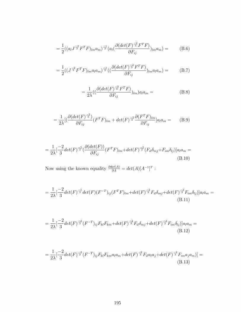
=1
2((alJ
−23 F TF )lmam)
−12 (al(
∂(det(F )−23 F TF )
∂Fij)lmam) = (B.6)
=1
2((J
−23 F TF )lmalam)
−12 ((
∂(det(F )−23 F TF )
∂Fij)lmalam) = (B.7)
=1
2λ((∂(det(F )
−23 F TF )
∂Fij)lm)alam = (B.8)
=1
2λ[(∂(det(F )
−23 )
∂Fij(F TF )lm + det(F )
−23∂(F TF )lm∂Fij
]alam = (B.9)
=1
2λ[−2
3det(F )
−53 (∂(det(F ))
∂Fij(F TF )lm+det(F )
−23 (Filδmj+Fimδlj)]alam =
(B.10)
Now using the known equality ∂det(A)∂A
= det(A)[A−1]T :
=1
2λ[−2
3det(F )
−53 det(F )(F−T )ij(F
TF )lm+det(F )−23 Filδmj+det(F )
−23 Fimδlj)]alam =
(B.11)
=1
2λ[−2
3det(F )
−23 (F−T )ijFklFkm+det(F )
−23 Filδmj+det(F )
−23 Fimδlj)]alam =
(B.12)
=1
2λ[−2
3det(F )
−23 (F−T )ijFklFkmalam+det(F )
−23 Filalaj+det(F )
−23 Fimajam)] =
(B.13)
195
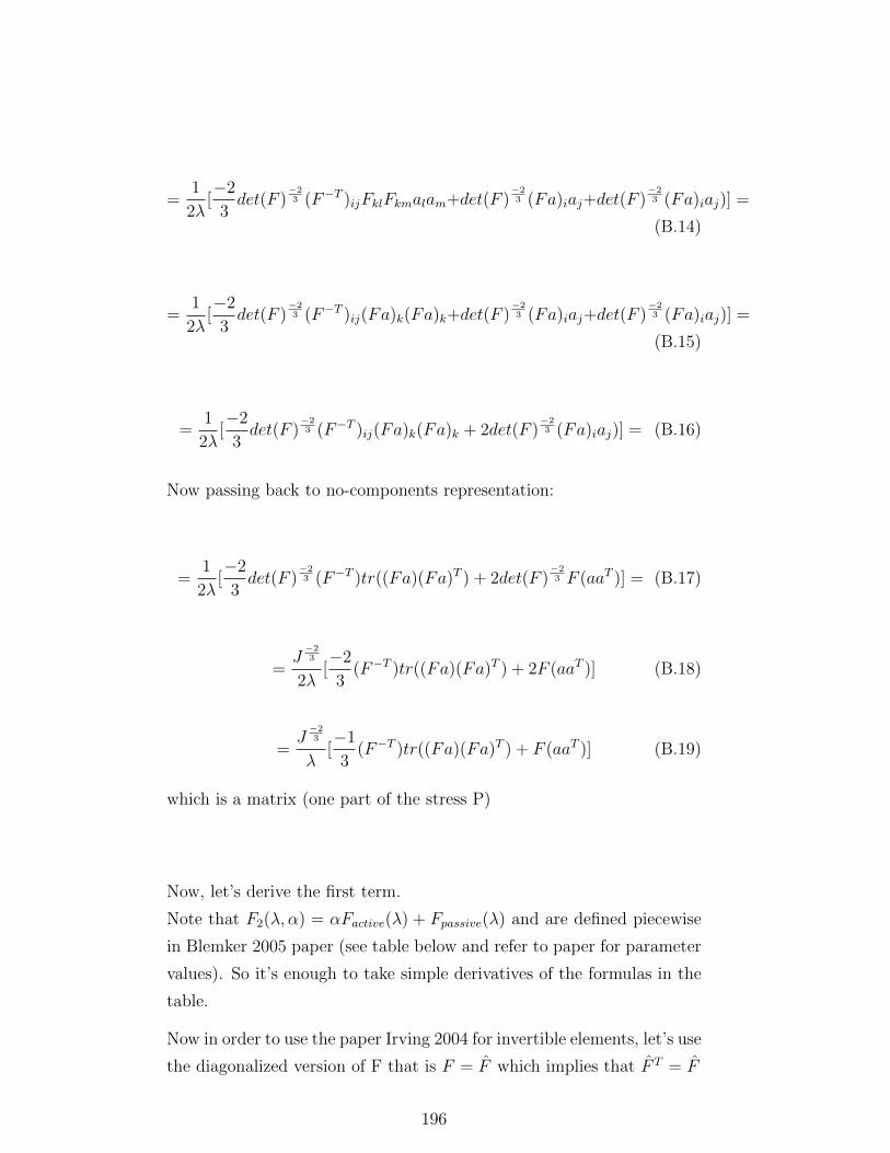
=1
2λ[−2
3det(F )
−23 (F−T )ijFklFkmalam+det(F )
−23 (Fa)iaj+det(F )
−23 (Fa)iaj)] =
(B.14)
=1
2λ[−2
3det(F )
−23 (F−T )ij(Fa)k(Fa)k+det(F )
−23 (Fa)iaj+det(F )
−23 (Fa)iaj)] =
(B.15)
=1
2λ[−2
3det(F )
−23 (F−T )ij(Fa)k(Fa)k + 2det(F )
−23 (Fa)iaj)] = (B.16)
Now passing back to no-components representation:
=1
2λ[−2
3det(F )
−23 (F−T )tr((Fa)(Fa)T ) + 2det(F )
−23 F (aaT )] = (B.17)
=J−23
2λ[−2
3(F−T )tr((Fa)(Fa)T ) + 2F (aaT )] (B.18)
=J−23
λ[−1
3(F−T )tr((Fa)(Fa)T ) + F (aaT )] (B.19)
which is a matrix (one part of the stress P)
Now, let’s derive the first term.
Note that F2(λ, α) = αFactive(λ) + Fpassive(λ) and are defined piecewise
in Blemker 2005 paper (see table below and refer to paper for parameter
values). So it’s enough to take simple derivatives of the formulas in the
table.
Now in order to use the paper Irving 2004 for invertible elements, let’s use
the diagonalized version of F that is F = F which implies that F T = F
196

Figure B.1: Formulas reproduced from Blemker 2005 paper.
197
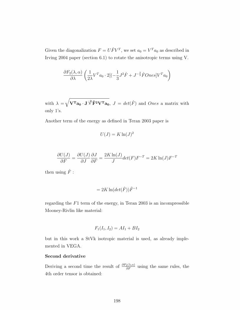
Given the diagonalization F = UFV T , we set a0 = V Ta0 as described in
Irving 2004 paper (section 6.1) to rotate the anisotropic terms using V.
∂F2(λ, α)
∂λ
(1
2λV Ta0 · 2[(−1
3J2F + J−
23 FOnes]V Ta0
)
with λ =
√VTa0 · J
−23 F2VTa0, J = det(F ) and Ones a matrix with
only 1’s.
Another term of the energy as defined in Teran 2003 paper is
U(J) = K ln(J)2
∂U(J)
∂F=∂U(J)
∂J
∂J
∂F=
2K ln(J)
Jdet(F )F−T = 2K ln(J)F−T
then using F :
= 2K ln(det(F ))F−1
regarding the F1 term of the energy, in Teran 2003 is an incompressible
Mooney-Rivlin like material:
F1(I1, I2) = AI1 +BI2
but in this work a StVk isotropic material is used, as already imple-
mented in VEGA.
Second derivative
Deriving a second time the result of ∂F2(λ,α)∂F
using the same rules, the
4th order tensor is obtained:
198

∂2F2(λ, α)
∂F 2=
= −2
9J−23 (F−T )ij(a0 · J
−23 F TFa0)
−12lm (F−T )ij(Fa)k(Fa)k
− 2
3J−23 (F−T )ij(a0 · J
−23 F TFa0)
−12lm (Fa)iaj
199

Appendix C
Material Derivation (cont.)
C.1 Derivation of dPdF for StVk material
Derivation of the Piola stress for StVk stress P(F):
P(F) = F[2µE + λtr(E)I] (C.1)
Some known identities used:
∂Fij
∂Fpq
= δipδjq
where δmn is the Dirac’s delta that evaluates to 1 IFF m = n , 0 other-
wise.
Trace in index notation:
tr(FTF) = tr((FTF)lm) = tr(FTlkFkm) = FT
lkFkl = FklFkl
Derivative of the trace:
∂tr(FTF)
∂F=∂FklFkl
∂Fpq
=∂Fkl
∂Fpq
Fkl +∂Fkl
∂Fpq
Fkl = 2δkpδlqFkl = 2Fpq
Which is correct considering that in Sifakis notes it results 2F .
200

Derivative of FTF
∂(FTF)
∂F=∂(FTF)lm∂Fpq
=∂(FT
lkFkm)
∂Fpq
=∂(FT
lk)
∂Fpq
Fkm +∂(Fkm)
∂Fpq
FTlk =
= δkpδlqFkm + δkpδmqFkl = δlqFpm + δmqFpl
Full derivation :
∂P(F)
∂F=∂(F[2µE + λtr(E)I])
∂F= (C.2)
∂(2µFE + λtr(E)F)
∂F= (C.3)
∂(2µF12(FTF− I) + λ1
2tr(FTF− I)F)
∂F= (C.4)
∂(µF(FTF− I) + λ12tr(FTF− I)F)
∂F= (C.5)
µ∂(F(FTF− I))
∂F+
1
2λ∂(tr(FTF− I)F)
∂F= (C.6)
At this point let’s call A the first term and B the second and solve them
separately.
A:
µ∂(F(FTF− I))
∂F= (C.7)
µ∂(FFTF− F)
∂F= (C.8)
201
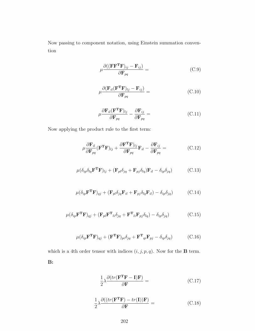
Now passing to component notation, using Einstein summation conven-
tion
µ∂((FFTF)ij − Fij)
∂Fpq
= (C.9)
µ∂(Fil(F
TF)lj − Fij)
∂Fpq
= (C.10)
µ∂Fil(F
TF)lj∂Fpq
− ∂Fij
∂Fpq
= (C.11)
Now applying the product rule to the first term:
µ∂Fil
∂Fpq
(FTF)lj +∂FTF)lj∂Fpq
Fil −∂Fij
∂Fpq
= (C.12)
µ(δipδlqFTF)lj + (Fplδjq + Fpjδlq)Fil − δipδjq) (C.13)
µ(δipFTF)qj + (FplδjqFil + FpjδlqFil)− δipδjq) (C.14)
µ(δipFTF)qj + (FplF
Tliδjq + FT
liFpjδlq)− δipδjq) (C.15)
µ(δipFTF)qj + (FTF)piδjq + FT
qiFpj − δipδjq) (C.16)
which is a 4th order tensor with indices (i, j, p, q). Now for the B term.
B:
1
2λ∂(tr(FTF− I)F)
∂F= (C.17)
1
2λ∂((tr(FTF)− tr(I))F)
∂F= (C.18)
202
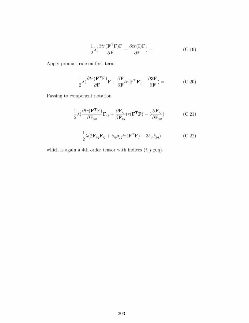
1
2λ(∂tr(FTF)F
∂F− ∂tr(I)F
∂F) = (C.19)
Apply product rule on first term
1
2λ(∂tr(FTF)
∂FF +
∂F
∂Ftr(FTF)− ∂3F
∂F) = (C.20)
Passing to component notation
1
2λ(∂tr(FTF)
∂Fpq
Fij +∂Fij
∂Fpq
tr(FTF)− 3∂Fij
∂Fpq
) = (C.21)
1
2λ(2FpqFij + δipδjqtr(F
TF)− 3δipδjq) (C.22)
which is again a 4th order tensor with indices (i, j, p, q).
203

Appendix D
EngD Experience Conclusions
As a general conclusion, overall the experience of doing an engineering
doctorate (EngD) was extremely valuable, mostly for the fact of being
immersed in a production environment which was the right ecosystem
to develop research ideas that could have a real life impact. Below are
summarized some of the lessons learned in my journey, together with
recommendations for future students who intend to take the research
path of an EngD.
Unless strictly necessary, it is advisable to not start coding from scratch
neither basic nor complex libraries that have already an efficient open
source implementation, especially for research papers: an EngD is not a
programming exercise. The reason is that writing really efficient APIs
not only requires extremely solid software engineering expertise, but also
takes significant time which would be subtracted from the real occupation
of any researcher: doing research. Luckily there are numerous open
source projects in the computer graphics community which are freely
available under different kinds of licenses.
At the same time though, it is of capital importance to start implement-
ing prototypes as soon as possible and win the temptation of first reading
and studying every single paper on the topic. A good initial literature
review is essential to put order and hierarchy of importance in the vast
amount of knowledge available on a research topic, but thinking that a
204

good innovative idea will come only after an exhaustive analysis of all the
papers is just an illusion. The most productive and original ideas come
generally either after long term focus on a very narrow area or through
the influence of research developed in other fields, often totally different
from computer graphics (i.e. biology, chemistry, artificial intelligence).
When doing Research and Development (RnD) it is easy to isolate one-
self from the rest of the team because complex problems require persis-
tent mental effort spread often across several months. It is fundamental
though to keep maintaining the feedback loop between supervisors and
especially people involved in production bouncing off ideas regularly.
This can be obtained through daily or weekly scrums and regular video
calls. It is common to arrive at dead ends in research: it was often the
case in my experience to get new fresh perspectives and valuable sug-
gestions from people working in other departments of the company, not
biased about the problem I was trying to solve.
When choosing a research project and during the inevitable iterations
and adjustments that will follow, it is important to always try and see
the implications of the work on the long term in the future and its place
in the global pipeline. The output of the character deformation stage for
example affects deeply the grooming department stage so keeping the
big picture in mind helped taking some technical decisions over others.
For this reason I recommend creating flexible plans and revise them with
supervisors regularly, making sure that every week brings some form of
progress towards either a new goal or the resolution of existing problems.
In general, the persistent awareness that it is necessary to fail early and
often while being at the same time ”micro-ambitious”, constituted the
main mindset I adopted in the many and inevitable periods of setbacks.
205