Adaptive Pricing in Multi-Agent Supply Chain Markets

using Economic Regimes

Alexander Hogenboom∗ Wolfgang Ketter† Jan van Dalen‡

Uzay Kaymak§ John Collins¶ Alok Gupta‖

Student-authored paper

Abstract

In today’s complex supply chain markets, information systems are crucial for effec-

tive supply chain management, supporting complex decision processes that can improve

the agility of organizations. The highly competitive nature of today’s complex supply

chain markets requires sophisticated dynamic product pricing that can adapt quickly

to dynamic market conditions, competitors’ strategies, etcetera. We propose a product

pricing approach which estimates the parameters of the distribution of all prices of-

fered by suppliers in real-time, based on available information. The relations between

price distributions and available information are dynamically modeled by accounting

for customer feedback and by characterizing different market conditions using economic

regimes. Given the parametric approximations of price distributions, offer acceptance

probabilities are estimated using a closed-form mathematical expression, which is used

to determine the price that is expected to yield a desired sales quota. We validate

∗Erasmus Sch. of Econ., Erasmus University Rotterdam, hogenboom@ese.eur.nl†Rotterdam Sch. of Mgmt., Erasmus University Rotterdam, wketter@rsm.nl‡Rotterdam Sch. of Mgmt., Erasmus University Rotterdam, jdalen@rsm.nl§Erasmus Sch. of Econ., Erasmus University Rotterdam, kaymak@ese.eur.nl¶Computer Science and Engr., University of Minnesota, jcollins@cs.umn.edu‖Carlson Sch. of Mgmt., University of Minnesota, agupta@csom.umn.edu

our methods by presenting experimental results from a testbed derived from the Trad-

ing Agent Competition for Supply Chain Management (TAC SCM). When competing

against world’s leading TAC SCM agents, performance significantly improves; bid effi-

ciency increases and profits more than double.

1 Introduction

Supply chain markets are ubiquitous in today’s global economy. In a supply chain, raw

materials are converted into products and distributed to final users [11]. As today’s supply

chains are complex logistics systems which can encompass many interrelated entities, effec-

tive Supply Chain Management (SCM), focused flexible and dynamic relationships among

entities in the supply chain, is vital to the competitiveness of manufacturers within this

chain. Effective SCM enables manufacturers to respond to changing market demands in a

timely and cost effective manner [5] and can thus improve the agility of supply chain entities.

A challenge in this context is dynamic product pricing. When flexible and dynamic relation-

ships between supply chain entities stimulate manufacturers to compete for customer orders,

optimal product prices must account for numerous factors, such as competitors’ strategies

or market conditions [9, 22, 23, 34, 37]. This requires a sophisticated dynamic product pric-

ing approach, possibly facilitated by automated decision support systems that rely on data

retrieved from information systems.

Information systems can provide valuable inputs for the product pricing process as they

can encompass a large variety of data. However, in real-time applications, information rele-

vant to product pricing may not be (fully) available, as for instance competitors’ strategies

may not be observable. Despite the limited visibility of market characteristics, real-time

adaptation to changing market circumstances is desired in today’s complex supply chain

markets. This suggests a need for information systems to be used in a more creative way

in order to augment their utility in supporting decision making processes. Therefore, we

investigate how dynamic pricing decisions using estimations of economic regimes – charac-

terizations of market conditions [16, 17, 20] – can contribute to profit maximization. We

validate our approach in a highly competitive setting in the Trading Agent Competition for

Supply Chain Management (TAC SCM) [7], which has been organized since 2003 to promote

high quality research into trading agents in supply chain environments. In TAC SCM, several

manufacturers (autonomous software trading agents) compete in a component procurement

market and in a sales market where assembled products are sold through reverse auctions in

response to requests for quotes (RFQs). The market is only partially observable.

The paper is organized as follows. In Section 2, we discuss related work on dynamic

product pricing. Our own product pricing approach is introduced in Section 3. In Section 4,

adaptivity is introduced to this approach. We evaluate the novel approach in the TAC SCM

in Section 5 and we conclude in Section 6.

2 Related Work

A common and intuitive approach for effective dynamic product pricing accounts for the

probability that a customer actually accepts the offer and hence proceeds to buy the product

for the offered price. A good approximation of this probability can help a seller assess how

sales targets can be met. Recent research suggests viability of this approach. For instance,

in [9], products are priced using a dynamic pricing algorithm which considers an estimated

distribution of the buyer reservation price for products of a seller. Reversing the cumulative

form of this distribution yields a function expressing the proportion of buyers willing to pay

the seller a specified price, which can also be interpreted as the probability that a customer

accepts an offered price. This function can subsequently be used to determine the price

expected to yield a specified sales quota. In [42], estimated distributions of buyer’s private

values are used in a similar way.

Another way of modeling acceptance probabilities is by using linear regression on data

points representing recent offer prices and their resulting acceptance rate [32]. Acceptance

probability distributions could also be trained off-line [2]. Another option is to try to model

the decision function of the accepting entities, based on their decision histories, e.g., using

Chebychev polynomials [34].

Related work suggests that other aspects besides acceptance probabilities are relevant in

the product pricing process. For instance, in case of known demand and uncertain supply, a

responsive pricing policy, in which the retail price is determined after observing the realized

supply, results in a higher expected profit than a pricing policy in which the realized supply

is not taken into account [39]. Consequently, modeling expected or observed supply-side

behavior in the product pricing process could contribute to profit maximization. Further-

more, current and future offers of competitors (outside options) could be considered [22, 23].

In [37], outside options are considered as well by quantifying both the price change of a

product itself and the relative price of competing products in a price elasticity. Using sce-

nario analysis for distinguishing between various situations of price elasticity (i.e., market

conditions), the optimal pricing policy is selected.

Market conditions can also be accounted for using economic regimes [16, 17, 20]. Regimes

are sets of conditions of a system or process and provide an intuitive way of conditioning

behavior in different scenarios. Several approaches to regime identification and prediction

have been proposed in different contexts [1, 13, 14, 29]. In an economic context, the ability of

decision makers to correctly identify the current regime and predict the onset of a new regime

is crucial in order to prevent over- or underreaction to market conditions [25]. Economic

regimes can guide tactical (e.g., product pricing) and strategic sales decisions (e.g., product

mix and production planning) [16, 17, 20].

Past research describes several aspects in the product pricing process. Using expected

or observed supply-side behavior, current and future offers of competitors (or competitors’

pricing strategies), along with perceived market conditions (characterized using economic

regimes) to estimate the probability that a customer accepts a price appears to be a viable

strategy in dynamically determining the optimal product prices. However, a dynamic prod-

uct pricing approach that takes all these findings into account, and is thus able to adapt

to ever-changing market circumstances such as those in highly competitive complex supply

chains, is yet to be proposed.

3 Product Pricing based on Offer Price Distributions

Manufacturers of durable goods typically sell their products in oligopolistic markets with

differentiated customer demand. Knowledge about competitors’ procurement, production

and pricing decisions is generally not available. Such knowledge can at most indirectly

be inferred from unexpected increases or decreases of the volume or profitability of one’s

own sales. Customers may be expected to simply purchase the lowest priced product from

any offer of equally preferred product specifications, but aggregate demand will vary over

time with respect to volume as well as quality. Accurate predictions of the price at which

customers are willing to accept offered products are essential to maintain sustainable market

positions.

In this section, we develop a model for the probability that offers are accepted given a

certain price. The model is based on the idea that past information about product sales

and prices can be used to infer the distribution of offered prices in the market. Real-time

application of this model requires flexible updating of the parameters involved, for which we

propose Artificial Neural Networks (ANNs).

3.1 General Framework

Given the considerations presented in Section 2, we propose to approximate customer offer

acceptance probabilities by taking into account the distribution of all offered prices, because

we can thus model the unobservable decision making processes of all traders and obtain

a complete estimation of customer acceptance probabilities. Using, e.g., linear regression

on recent offer prices as proposed in [32] would imply a less accurate model of supply-side

behavior and competitors’ pricing strategies. Furthermore, modeling offer price distributions

rather than individual – potentially non-occurring – offer prices (as proposed in [22]) yields

a more robust approach.

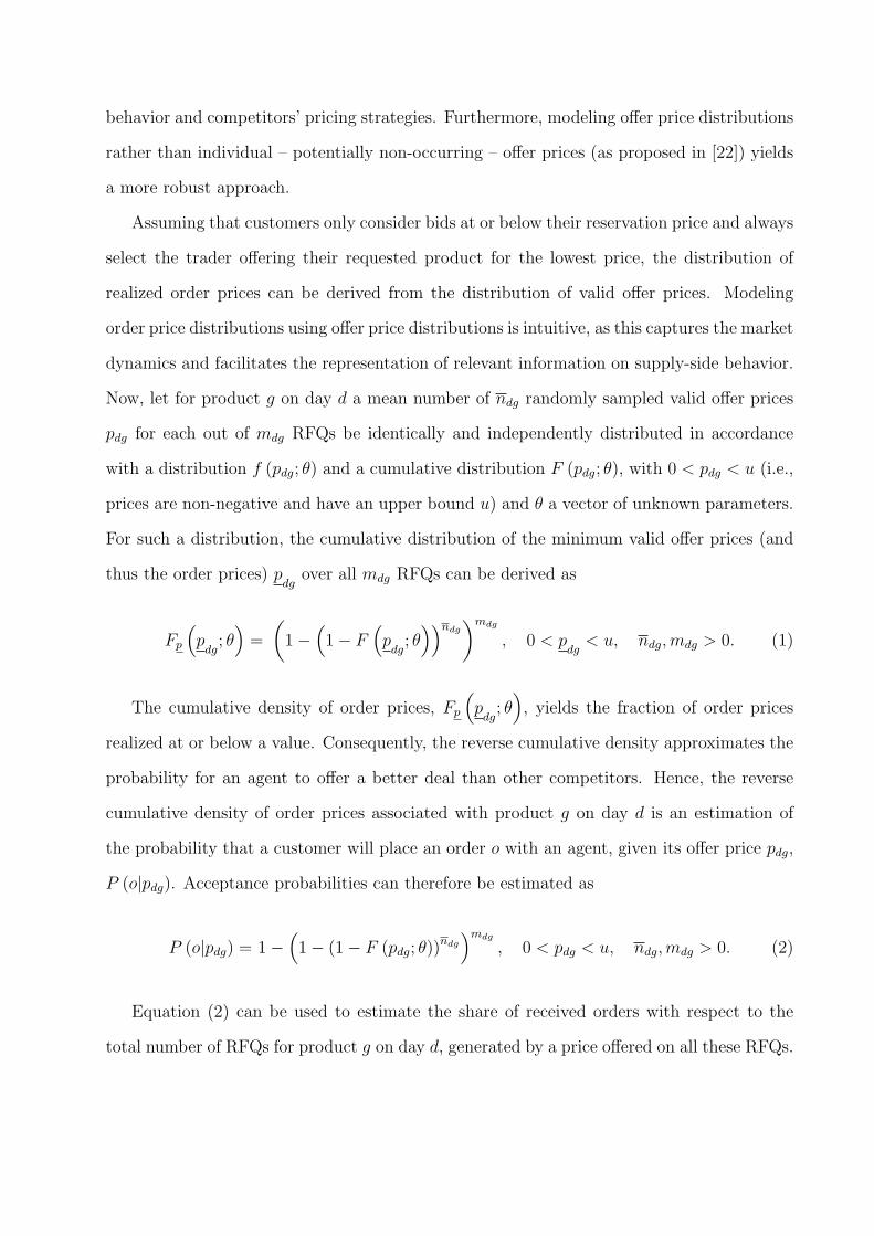
Assuming that customers only consider bids at or below their reservation price and always

select the trader offering their requested product for the lowest price, the distribution of

realized order prices can be derived from the distribution of valid offer prices. Modeling

order price distributions using offer price distributions is intuitive, as this captures the market

dynamics and facilitates the representation of relevant information on supply-side behavior.

Now, let for product g on day d a mean number of ndg randomly sampled valid offer prices

pdg for each out of mdg RFQs be identically and independently distributed in accordance

with a distribution f (pdg; θ) and a cumulative distribution F (pdg; θ), with 0 < pdg < u (i.e.,

prices are non-negative and have an upper bound u) and θ a vector of unknown parameters.

For such a distribution, the cumulative distribution of the minimum valid offer prices (and

thus the order prices) pdg

over all mdg RFQs can be derived as

Fp

(p

dg; θ

)=

(1−

(1− F

(p

dg; θ

))ndg

)mdg

, 0 < pdg

< u, ndg,mdg > 0. (1)

The cumulative density of order prices, Fp

(p

dg; θ

), yields the fraction of order prices

realized at or below a value. Consequently, the reverse cumulative density approximates the

probability for an agent to offer a better deal than other competitors. Hence, the reverse

cumulative density of order prices associated with product g on day d is an estimation of

the probability that a customer will place an order o with an agent, given its offer price pdg,

P (o|pdg). Acceptance probabilities can therefore be estimated as

P (o|pdg) = 1−(1− (1− F (pdg; θ))

ndg

)mdg

, 0 < pdg < u, ndg,mdg > 0. (2)

Equation (2) can be used to estimate the share of received orders with respect to the

total number of RFQs for product g on day d, generated by a price offered on all these RFQs.

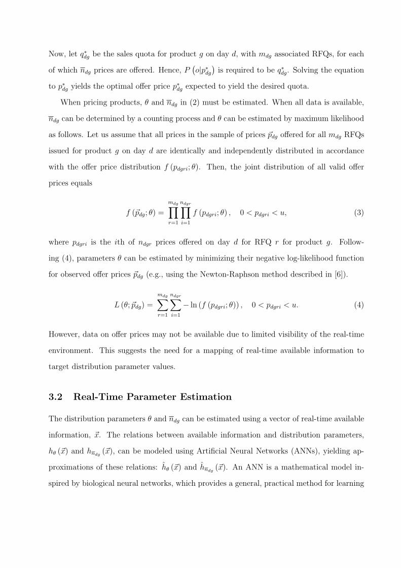
Now, let q∗dg be the sales quota for product g on day d, with mdg associated RFQs, for each

of which ndg prices are offered. Hence, P(o|p∗dg

)is required to be q∗dg. Solving the equation

to p∗dg yields the optimal offer price p∗dg expected to yield the desired quota.

When pricing products, θ and ndg in (2) must be estimated. When all data is available,

ndg can be determined by a counting process and θ can be estimated by maximum likelihood

as follows. Let us assume that all prices in the sample of prices ~pdg offered for all mdg RFQs

issued for product g on day d are identically and independently distributed in accordance

with the offer price distribution f (pdgri; θ). Then, the joint distribution of all valid offer

prices equals

f (~pdg; θ) =

mdg∏r=1

ndgr∏i=1

f (pdgri; θ) , 0 < pdgri < u, (3)

where pdgri is the ith of ndgr prices offered on day d for RFQ r for product g. Follow-

ing (4), parameters θ can be estimated by minimizing their negative log-likelihood function

for observed offer prices ~pdg (e.g., using the Newton-Raphson method described in [6]).

L (θ; ~pdg) =

mdg∑r=1

ndgr∑i=1

− ln (f (pdgri; θ)) , 0 < pdgri < u. (4)

However, data on offer prices may not be available due to limited visibility of the real-time

environment. This suggests the need for a mapping of real-time available information to

target distribution parameter values.

3.2 Real-Time Parameter Estimation

The distribution parameters θ and ndg can be estimated using a vector of real-time available

information, ~x. The relations between available information and distribution parameters,

hθ (~x) and hndg(~x), can be modeled using Artificial Neural Networks (ANNs), yielding ap-

proximations of these relations: hθ (~x) and hndg(~x). An ANN is a mathematical model in-

spired by biological neural networks, which provides a general, practical method for learning

real-valued, discrete-valued, and vector-valued functions over continuous and discrete-valued

attributes from examples in order to facilitate regression or classification [27]. The model

consists of interconnecting artificial neurons (nodes), ordered into an input layer, hidden

layers, and an output layer.

Due to the ability of an ANN to capture complex nonlinear relations, we can replace

parameter estimation using (4) with such a model, albeit with different inputs (i.e., real-

time available data). Representing the unknown relations between distribution parameters

and real-time available data using ANNs also brings the attractive feature of fast evaluation

of these functions, which is crucial for real-time product pricing. Other advantages include

robustness to noise in the training data [27], the possibility to introduce adaptivity by adjust-

ing the weights of each node’s inputs on-the-fly using newly obtained examples (if any), and

the fact that ANNs have proven to be useful for economic forecasts in various domains [22].

Moreover, our experimental results regarding TAC SCM show that ANNs better capture the

relation between data and distribution parameters than, e.g., linear regression.

We propose to use a specific type of ANN: a radial basis function network (RBFN),

because this type of ANN can be designed and trained in a fraction of the time it takes

to train standard feed-forward back-propagation ANNs [27]. A RBFN is a two-layer ANN

consisting of a hidden layer and an output layer. The activation function in each hidden unit

h is a local function Kh (d (~xh, ~x)), where ~x is a vector of features, ~xh is the center of ~x, and

d (~xh, ~x) is the “distance” between ~xh and ~x. Kh(z) is a function whose value is a maximum

when z = 0, and approaches zero for large values of z. The local functions in the hidden

layer typically are Gaussians, centered at ~xh with variance σ2h. The number of Gaussians H

is subject to optimization and their centers can be determined by clustering the data, using

for example the k-means algorithm [24]. The network’s output for an instance ~x, h (~x), is a

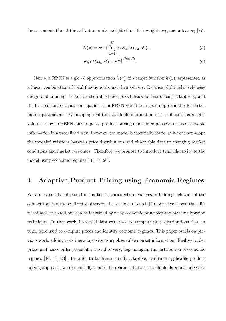
linear combination of the activation units, weighted for their weights wh, and a bias w0 [27]:

h (~x) = w0 +H∑

h=1

whKh (d (xh, ~x)) , (5)

Kh (d (xh, ~x)) = e1

2σ2h

d2(xh,~x). (6)

Hence, a RBFN is a global approximation h (~x) of a target function h (~x), represented as

a linear combination of local functions around their centers. Because of the relatively easy

design and training, as well as the robustness, possibilities for introducing adaptivity, and

the fast real-time evaluation capabilities, a RBFN would be a good approximator for distri-

bution parameters. By mapping real-time available information to distribution parameter

values through a RBFN, our proposed product pricing model is responsive to this observable

information in a predefined way. However, the model is essentially static, as it does not adapt

the modeled relations between price distributions and observable data to changing market

conditions and market responses. Therefore, we propose to introduce true adaptivity to the

model using economic regimes [16, 17, 20].

4 Adaptive Product Pricing using Economic Regimes

We are especially interested in market scenarios where changes in bidding behavior of the

competitors cannot be directly observed. In previous research [20], we have shown that dif-

ferent market conditions can be identified by using economic principles and machine learning

techniques. In that work, historical data were used to compute price distributions that, in

turn, were used to compute prices and identify economic regimes. This paper builds on pre-

vious work, adding real-time adaptivity using observable market information. Realized order

prices and hence order probabilities tend to vary, depending on the distribution of economic

regimes [16, 17, 20]. In order to facilitate a truly adaptive, real-time applicable product

pricing approach, we dynamically model the relations between available data and price dis-

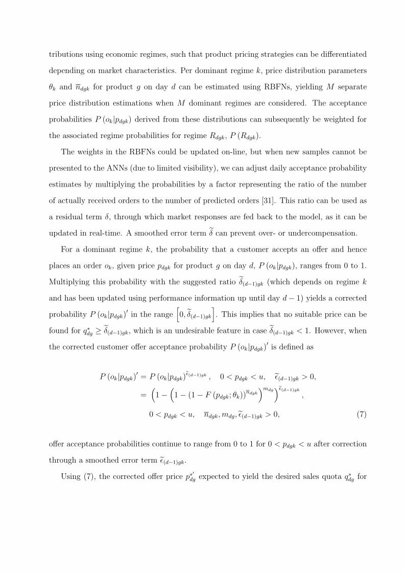
tributions using economic regimes, such that product pricing strategies can be differentiated

depending on market characteristics. Per dominant regime k, price distribution parameters

θk and ndgk for product g on day d can be estimated using RBFNs, yielding M separate

price distribution estimations when M dominant regimes are considered. The acceptance

probabilities P (ok|pdgk) derived from these distributions can subsequently be weighted for

the associated regime probabilities for regime Rdgk, P (Rdgk).

The weights in the RBFNs could be updated on-line, but when new samples cannot be

presented to the ANNs (due to limited visibility), we can adjust daily acceptance probability

estimates by multiplying the probabilities by a factor representing the ratio of the number

of actually received orders to the number of predicted orders [31]. This ratio can be used as

a residual term δ, through which market responses are fed back to the model, as it can be

updated in real-time. A smoothed error term δ can prevent over- or undercompensation.

For a dominant regime k, the probability that a customer accepts an offer and hence

places an order ok, given price pdgk for product g on day d, P (ok|pdgk), ranges from 0 to 1.

Multiplying this probability with the suggested ratio δ(d−1)gk (which depends on regime k

and has been updated using performance information up until day d− 1) yields a corrected

probability P (ok|pdgk)′ in the range

[0, δ(d−1)gk

]. This implies that no suitable price can be

found for q∗dg ≥ δ(d−1)gk, which is an undesirable feature in case δ(d−1)gk < 1. However, when

the corrected customer offer acceptance probability P (ok|pdgk)′ is defined as

P (ok|pdgk)′ = P (ok|pdgk)

ε(d−1)gk , 0 < pdgk < u, ε(d−1)gk > 0,

=(1−

(1− (1− F (pdgk; θk))

ndgk

)mdg)ε(d−1)gk

,

0 < pdgk < u, ndgk,mdg, ε(d−1)gk > 0, (7)

offer acceptance probabilities continue to range from 0 to 1 for 0 < pdgk < u after correction

through a smoothed error term ε(d−1)gk.

Using (7), the corrected offer price p∗′

dg expected to yield the desired sales quota q∗dg for

product g on day d can be defined for each dominant regime k, by requiring P(ok|p∗′dgk

)′for

that product on that day to be q∗dg. Solving the equation to p∗′

dgk yields the optimal corrected

offer price p∗′

dgk expected to yield the desired quota q∗dg under dominant regime k. When

these corrected prices are then weighted for their associated regime probabilities P (Rdgk),

the corrected price p∗′

dg expected to yield the required quota can be obtained.

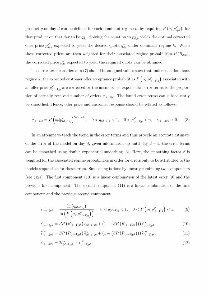
The error term considered in (7) should be assigned values such that under each dominant

regime k, the expected customer offer acceptance probabilities P(ok|p∗′(d−1)g

)associated with

an offer price p∗′

(d−1)g are corrected by the unsmoothed exponential error terms to the propor-

tion of actually received number of orders q(d−1)g. The found error terms can subsequently

be smoothed. Hence, offer price and customer response should be related as follows:

q(d−1)g = P(ok|p∗′(d−1)g

)ε(d−1)gk

, 0 < q(d−1)g < 1, 0 < p∗′

(d−1)g < u, ε(d−1)gk > 0. (8)

In an attempt to track the trend in the error terms and thus provide an accurate estimate

of the error of the model on day d, given information up until day d − 1, the error terms

can be smoothed using double exponential smoothing [3]. Here, the smoothing factor β is

weighted for the associated regime probabilities in order for errors only to be attributed to the

models responsible for these errors. Smoothing is done by linearly combining two components

(see (12)). The first component (10) is a linear combination of the latest error (9) and the

previous first component. The second component (11) is a linear combination of the first

component and the previous second component.

ε(d−1)gk =ln

(q(d−1)g

)

ln(P

(ok|p∗′(d−1)g

)) , 0 < q(d−1)g < 1, 0 < P(ok|p∗′(d−1)g

)< 1, (9)

ε ′(d−1)gk = βP

(R(d−1)gk

)ε(d−1)gk +

(1− (

βP(R(d−1)gk

)))ε ′(d−2)gk, (10)

ε ′′(d−1)gk = βP

(R(d−1)gk

)ε ′(d−1)gk +

(1− (

βP(R(d−1)gk

)))ε ′′(d−2)gk, (11)

ε(d−1)gk = 2ε ′(d−1)gk − ε ′′

(d−1)gk. (12)

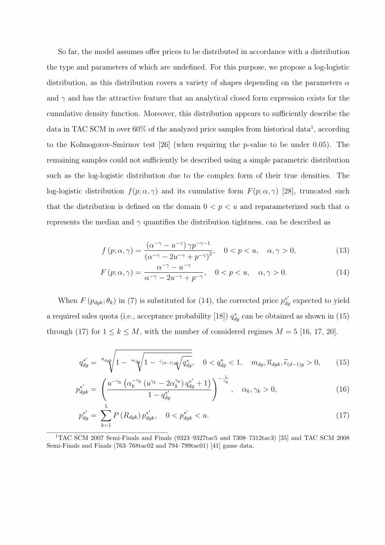
So far, the model assumes offer prices to be distributed in accordance with a distribution

the type and parameters of which are undefined. For this purpose, we propose a log-logistic

distribution, as this distribution covers a variety of shapes depending on the parameters α

and γ and has the attractive feature that an analytical closed form expression exists for the

cumulative density function. Moreover, this distribution appears to sufficiently describe the

data in TAC SCM in over 60% of the analyzed price samples from historical data1, according

to the Kolmogorov-Smirnov test [26] (when requiring the p-value to be under 0.05). The

remaining samples could not sufficiently be described using a simple parametric distribution

such as the log-logistic distribution due to the complex form of their true densities. The

log-logistic distribution f(p; α, γ) and its cumulative form F (p; α, γ) [28], truncated such

that the distribution is defined on the domain 0 < p < u and reparameterized such that α

represents the median and γ quantifies the distribution tightness, can be described as

f (p; α, γ) =(α−γ − u−γ) γp−γ−1

(α−γ − 2u−γ + p−γ)2 , 0 < p < u, α, γ > 0, (13)

F (p; α, γ) =α−γ − u−γ

α−γ − 2u−γ + p−γ, 0 < p < u, α, γ > 0. (14)

When F (pdgk; θk) in (7) is substituted for (14), the corrected price p∗′

dg expected to yield

a required sales quota (i.e., acceptance probability [18]) q∗dg can be obtained as shown in (15)

through (17) for 1 ≤ k ≤ M , with the number of considered regimes M = 5 [16, 17, 20].

q∗′

dg =ndgk

√1− mdg

√1− ε(d−1)gk

√q∗dg, 0 < q∗dg < 1, mdg, ndgk, ε(d−1)g > 0, (15)

p∗′

dgk =

(u−γk

(α−γk

k (uγk − 2αγk

k ) q∗′

dg + 1)

1− q∗′dg

)− 1γk

, αk, γk > 0, (16)

p∗′

dg =5∑

k=1

P (Rdgk) p∗′

dgk, 0 < p∗′

dgk < u. (17)

1TAC SCM 2007 Semi-Finals and Finals (9323–9327tac5 and 7308–7312tac3) [35] and TAC SCM 2008Semi-Finals and Finals (763–768tac02 and 794–799tac01) [41] game data.

Now, the model assumes a double-bounded log-logistic distribution to be underlying

offer prices, the parameters of which can be estimated real-time using RBFNs. The rela-

tion between available data and parameters is dynamically modeled using economic regimes

(characterizing market conditions) and error terms (accounting for customer feedback). The

proposed framework can now be evaluated in a highly competitive setting.

5 Testbed: The Trading Agent Competition for Sup-

ply Chain Management

The final framework can be evaluated by implementing the approach in the MinneTAC trad-

ing agent [8], developed for the Trading Agent Competition for Supply Chain Management

(TAC SCM). To this end, product pricing should be done using (9) through (12) and (15)

through (17). The αk, γk, and ndgk parameters for product g on day d for dominant regime

k are to be estimated using RBFNs. In the following sections, we give an overview of our

TAC SCM testbed.

5.1 TAC SCM Overview

The TAC SCM scenario models a supply chain for personal computers (PCs) over a simu-

lated one-year product life-cycle. Each of the 220 daily cycles is completed in 15 seconds of

real time. This supply chain consists of customers, manufacturers and suppliers (see Fig-

ure 1). Every day, customers issue RFQs for 16 different PC types, on which manufacturers

can bid. Customers always place an order with the manufacturer offering the requested

product for the lowest price (at or below their reservation price). Products are assembled by

the manufacturers using components procured from suppliers. Manufacturers are software

trading agents developed by competing teams, maximizing their profit over a game. Major

challenges include limited visibility of the market, limited time for decision-making, and the

need to coordinate decisions across the supply chain. Real-time available data consists of

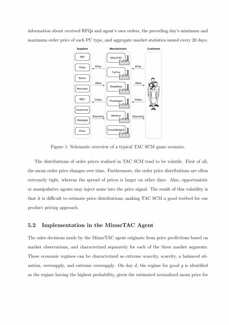
information about received RFQs and agent’s own orders, the preceding day’s minimum and

maximum order price of each PC type, and aggregate market statistics issued every 20 days.

Figure 1: Schematic overview of a typical TAC SCM game scenario.

The distributions of order prices realized in TAC SCM tend to be volatile. First of all,

the mean order price changes over time. Furthermore, the order price distributions are often

extremely tight, whereas the spread of prices is larger on other days. Also, opportunistic

or manipulative agents may inject noise into the price signal. The result of this volatility is

that it is difficult to estimate price distributions, making TAC SCM a good testbed for our

product pricing approach.

5.2 Implementation in the MinneTAC Agent

The sales decisions made by the MinneTAC agent originate from price predictions based on

market observations, and characterized separately for each of the three market segments.

These economic regimes can be characterized as extreme scarcity, scarcity, a balanced sit-

uation, oversupply, and extreme oversupply. On day d, the regime for good g is identified

as the regime having the highest probability, given the estimated normalized mean price for

that day. We estimate the normalized mid-range price, npdg, as the average of the double

exponentially smoothed normalized minimum and maximum price observed in the market.

The normalized price npdg for good g on day d is the ratio of actual price to nominal pro-

duction cost, which is the sum of the nominal costs of the parts required to build a product.

Normalized prices rarely fall below half of nominal cost, since this is the lowest cost available

from suppliers, and never rise above 1.25 of nominal cost, the upper bound on customer

reserve price.

A price density function has been modeled on historical normalized order price data us-

ing a Gaussian Mixture Model (GMM) [40] with a sufficient number of Gaussians (25 at

the moment), reflecting a balance between prediction accuracy and computational overhead.

Clustering these price distributions over time periods (using the k-means algorithm) has

yielded distinguishable statistical patterns: economic regimes. In TAC SCM, price informa-

tion is only available up until the preceding day. Hence, the MinneTAC agent estimates the

mean price of day d using an exponentially smoothed prediction of npdg and then returns

the regime probabilities for day d. When such an estimate is supplied to the model, the indi-

vidual Gaussians in the model are activated differentially, thus generating an expected price

distribution. Subsequently normalizing all clusters’ price densities enables determination of

regime probabilities. Future regime probabilities are determined by using Markov prediction

and Markov correction-prediction processes (for short-term and long-term decision making,

respectively) [19]. When current or future regime probabilities have been determined, prod-

ucts are priced using offer acceptance probabilities of these prices, such that a sales quota is

fulfilled.

In our benchmark sales configuration, price trends are estimated by the regime model.

Median product prices are estimated using a price-following approach implementing a double

exponential smoother. The trends and medians, along with cost estimates and resource

constraints, are inputs to a linear program that computes sales quotas that will maximize

profits over a medium-term time horizon. Given these daily sales quotas, optimal offer prices

are computed as the price that will sell the quota, given an order acceptance probability

curve. The acceptance probability curve is approximated using the estimated median price

and the curve’s slope in that median, estimated using exponentially smoothed prices. In order

to compensate for uncertainty in generated predictions, interval randomization is applied to

offer prices, which adds a slight variability to these prices. The estimated median is then

corrected using feedback derived from the desired optimized acceptance probability and the

associated true acceptance probability observed the next day.

The price distributions estimated by the GMM are updated on-line, but they do not

account for factors other than a mean price estimate and lack full adaptivity. In an attempt

to improve the product pricing process by combining regime information with real-time

available data, we replace the benchmark’s sales model with a system designed for Prod-

uct Pricing using Adaptive Real-time Regime-based Probability of Acceptance Estimations:

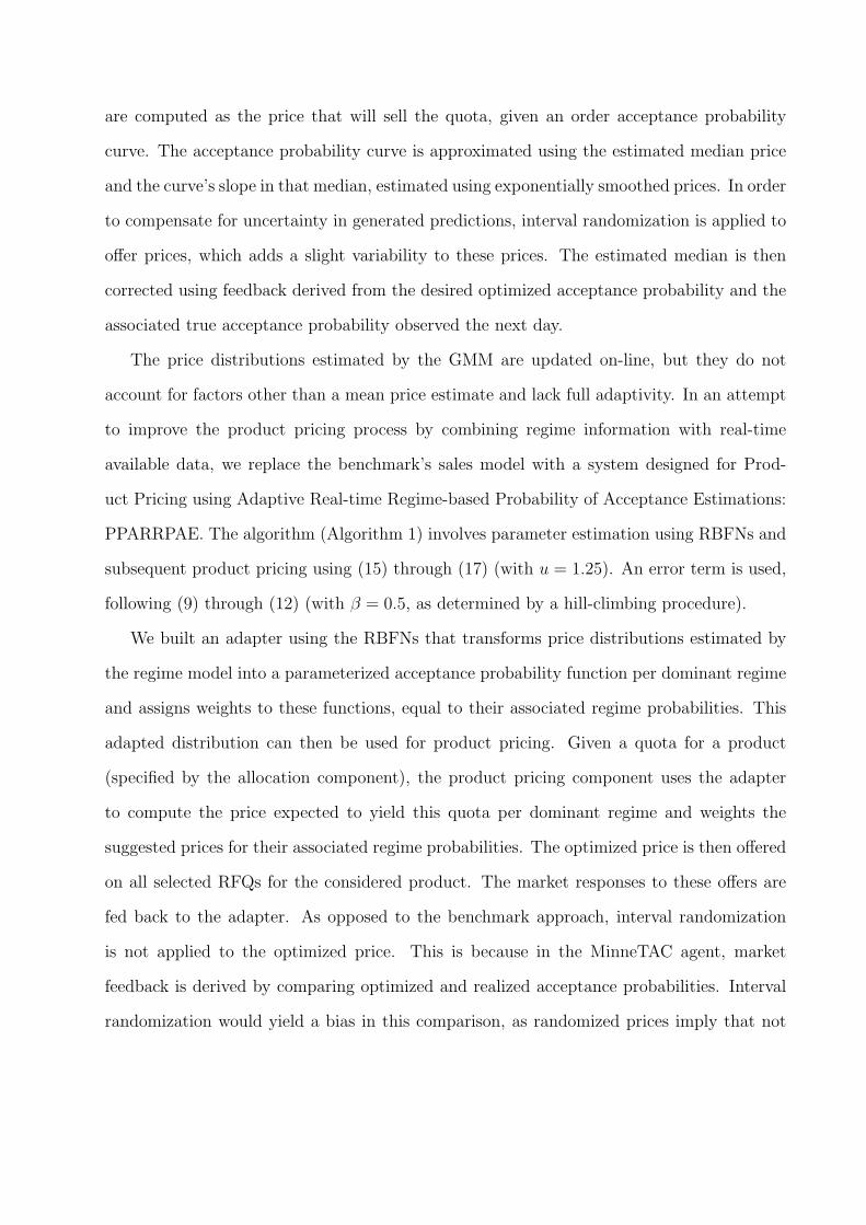
PPARRPAE. The algorithm (Algorithm 1) involves parameter estimation using RBFNs and

subsequent product pricing using (15) through (17) (with u = 1.25). An error term is used,

following (9) through (12) (with β = 0.5, as determined by a hill-climbing procedure).

We built an adapter using the RBFNs that transforms price distributions estimated by

the regime model into a parameterized acceptance probability function per dominant regime

and assigns weights to these functions, equal to their associated regime probabilities. This

adapted distribution can then be used for product pricing. Given a quota for a product

(specified by the allocation component), the product pricing component uses the adapter

to compute the price expected to yield this quota per dominant regime and weights the

suggested prices for their associated regime probabilities. The optimized price is then offered

on all selected RFQs for the considered product. The market responses to these offers are

fed back to the adapter. As opposed to the benchmark approach, interval randomization

is not applied to the optimized price. This is because in the MinneTAC agent, market

feedback is derived by comparing optimized and realized acceptance probabilities. Interval

randomization would yield a bias in this comparison, as randomized prices imply that not

foreach d in days doforeach g in products do

// Update error using last feedback, following (9) through (12)error = updateError(getFeedback(d− 1, g));// Retrieve data from regime model

regProbs = getRegProbs(d, g);regPriceDistr = getRegPriceDistr(d, g);trends = getTrends(d, g);// Estimate parameters using RBFNs

priceDistr = estParams(regPriceDistr, getData(d, g));// Determine median price using (15) through (17)median = priceForProb(0.5, priceDistr, error, regProbs);// Retrieve allocated quota

quota = getQuota(d, g, median, trends);// Determine price expected to yield quota using (15) through (17)price = priceForProb(quota, priceDistr, error, regProbs);// Bid optimized price on selected RFQs

priceProduct(d, g, price);end

endAlgorithm 1: The PPARRPAE approach.

every targeted acceptance probability associated with the offered price equals the optimized

acceptance probability.

5.3 Radial Basis Function Network Training

For each dominant regime k, a RBFN needs to be trained for estimating αk, γk, and ndgk for

product g on day d. Therefore, training and test datasets2 must be split into datasets per

dominant regime. These dominant regimes are identified by the current regime model. We

attempt to adapt regime-based price distributions done using the GMM implemented in the

MinneTAC agent in order for them to be useful in the daily product pricing process. Hence,

these regime-based price distributions should be used as RBFN inputs. For now, let these

distributions be described by their 10th, 50th, and 90th percentile and the spread of these

2TAC SCM 2007 Semi-Finals and Finals (9321–9328tac5 and 7306–7313tac3) [35] and TAC SCM 2008Semi-Finals and Finals (761–769tac02 and 792–800tac01) [41] game data. The first two games and the lastgame per server form the test set, the rest forms the training set.

percentiles.

The RBFNs should adapt these distributions using on-line available data. We use data

on product type, day, RFQ characteristics, and observable prices. Data on product type and

day is incorporated into our model because of the heterogeneity of products and the volatility

of their associated prices, mentioned in Section 5.1. RFQ characteristics are incorporated, as

(competitors’) pricing strategies – which related work discussed in Section 2 suggests to be

relevant when pricing products – are likely to depend on these characteristics. For example, a

reservation price provides an indication of the maximum price manufacturers will bid. Also,

the number of simultaneous similar bidding processes affects the associated revenues due to

their (partial) substitutivity [42]. Observable (historical) prices can also provide more insight

in competitors’ pricing strategies [22, 16, 17, 20]. The relevance of the on-line available data

mentioned is supported by initial experimental results on Pearson correlation between the

data and target distribution parameter values.

Using historical data, target parameter values can be determined by a counting process

(for ndgk) and by fitting distributions using (4) and (13) (for αk and γk). A typical training

dataset thus generated contains over 15,000 samples, a typical test dataset over 8,000. The

performance of RBFNs trained on the training set can be evaluated on the test set, as the

latter set is sufficiently large and representative [27]. For the resulting optimal values for

γk, the increment in γk needed to tighten the distribution increases as the distribution gets

tighter. Hence, as the required accuracy decreases for an increasing γk, the networks are

trained to predict the natural logarithm of γk.

For each regime-specific RBFN, the architecture is subject to optimization. The number

of inputs and the number of outputs are fixed. The number of hidden nodes is determined

using a hill-climbing procedure, with the objective to minimize the root mean squared devi-

ation (RMSD) on the test set, after training on the training set. The RMSD equals

RMSD =

√∑Ωω=1 (xω − xω)2

Ω, (18)

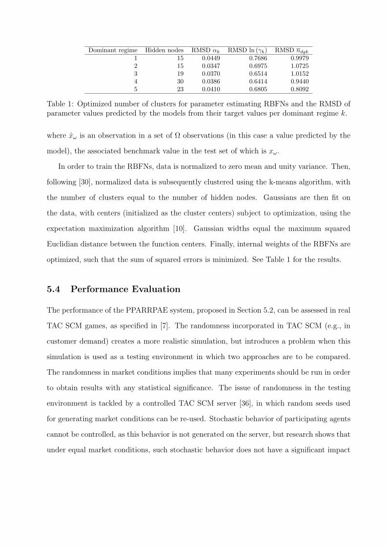
Dominant regime Hidden nodes RMSD αk RMSD ln (γk) RMSD ndgk

1 15 0.0449 0.7686 0.99792 15 0.0347 0.6975 1.07253 19 0.0370 0.6514 1.01524 30 0.0386 0.6414 0.94405 23 0.0410 0.6805 0.8092

Table 1: Optimized number of clusters for parameter estimating RBFNs and the RMSD ofparameter values predicted by the models from their target values per dominant regime k.

where xω is an observation in a set of Ω observations (in this case a value predicted by the

model), the associated benchmark value in the test set of which is xω.

In order to train the RBFNs, data is normalized to zero mean and unity variance. Then,

following [30], normalized data is subsequently clustered using the k-means algorithm, with

the number of clusters equal to the number of hidden nodes. Gaussians are then fit on

the data, with centers (initialized as the cluster centers) subject to optimization, using the

expectation maximization algorithm [10]. Gaussian widths equal the maximum squared

Euclidian distance between the function centers. Finally, internal weights of the RBFNs are

optimized, such that the sum of squared errors is minimized. See Table 1 for the results.

5.4 Performance Evaluation

The performance of the PPARRPAE system, proposed in Section 5.2, can be assessed in real

TAC SCM games, as specified in [7]. The randomness incorporated in TAC SCM (e.g., in

customer demand) creates a more realistic simulation, but introduces a problem when this

simulation is used as a testing environment in which two approaches are to be compared.

The randomness in market conditions implies that many experiments should be run in order

to obtain results with any statistical significance. The issue of randomness in the testing

environment is tackled by a controlled TAC SCM server [36], in which random seeds used

for generating market conditions can be re-used. Stochastic behavior of participating agents

cannot be controlled, as this behavior is not generated on the server, but research shows that

under equal market conditions, such stochastic behavior does not have a significant impact

on the agent profit levels [36]. The results presented in [36] also indicate that most significant

profit differences between agents can already be detected in approximately 40 games.

The performance of the PPARRPAE system can hence be evaluated in 40 experiment

sets on a controlled server. Each experiment set consists of a paired evaluation of the per-

formance of the benchmark and the PPARRPAE system under equal market characteristics.

The configurations can be tested in a highly competitive setting, in which MinneTAC com-

petes against world’s leading TAC SCM trading agents. TacTex [32] predicts demand using

a Bayesian approach and offer acceptance using linear regression, and adapts these offer

acceptance estimations to its opponents’ behavior. DeepMaize [21] uses a gradient descent

algorithm to find a set of offered prices in order to optimize the expected value of the resulting

orders. PhantAgent [38] and the CrocodileAgent [33] use simple heuristics for determining

what to sell for what price. Mertacor [4] predicts the winning bid per RFQ using a regres-

sion model, complemented with a price-following correction mechanism and the acceptance

probabilities are subsequently estimated using a k-nearest neighbors algorithm [24].

Performance differences should be assessed with respect to their statistical relevance.

This can be done using a paired, two-sided Wilcoxon signed-rank test [12, 15]. This is a

non-parametric test, which tests the hypothesis that the differences between paired obser-

vations are symmetrically distributed around a median equal to 0. If this null hypothesis is

rejected (at a significance level below 0.05), the compared sets of samples can be assumed

to be significantly different. This test would be suitable in this experimental setup, as the

distribution of the values to be compared is unknown.

Over all experiments, PPARRPAE outperforms the benchmark with respect to final bank

account balance, with significantly lower order volume (see Table 2). Generally, when using

PPARRPAE, the number of orders significantly decreases with over 21% (with a Wilcoxon

p-value of 0.0000), but the obtained orders yield a significant increase in final balances of

about 133% (with a p-value of 0.0004 for the Wilcoxon test) with respect to the benchmark.

The number of usable acceptance probability estimations significantly increases with approx-

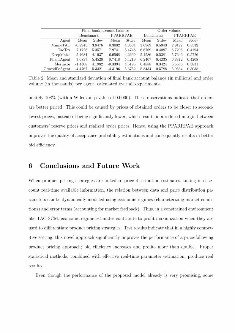
Final bank account balance Order volumeBenchmark PPARRPAE Benchmark PPARRPAE

Agent Mean Stdev Mean Stdev Mean Stdev Mean StdevMinneTAC -0.8945 3.9476 0.3002 4.3534 3.6969 0.5943 2.9127 0.5532

TacTex 7.1728 5.3571 7.9741 5.4748 6.6769 0.4087 6.7296 0.4194DeepMaize 5.4684 4.1937 6.9568 4.2669 5.4586 0.5381 5.7646 0.5726

PhantAgent 7.6837 5.4520 8.7418 5.4219 6.2407 0.4235 6.3372 0.4208Mertacor -1.4308 4.1982 -0.3394 4.5195 6.4888 0.3424 6.5655 0.3831

CrocodileAgent -4.4767 5.3321 -4.3196 5.3752 5.8434 0.5788 5.9564 0.5038

Table 2: Mean and standard deviation of final bank account balance (in millions) and ordervolume (in thousands) per agent, calculated over all experiments.

imately 108% (with a Wilcoxon p-value of 0.0000). These observations indicate that orders

are better priced. This could be caused by prices of obtained orders to be closer to second-

lowest prices, instead of being significantly lower, which results in a reduced margin between

customers’ reserve prices and realized order prices. Hence, using the PPARRPAE approach

improves the quality of acceptance probability estimations and consequently results in better

bid efficiency.

6 Conclusions and Future Work

When product pricing strategies are linked to price distribution estimates, taking into ac-

count real-time available information, the relation between data and price distribution pa-

rameters can be dynamically modeled using economic regimes (characterizing market condi-

tions) and error terms (accounting for market feedback). Thus, in a constrained environment

like TAC SCM, economic regime estimates contribute to profit maximization when they are

used to differentiate product pricing strategies. Test results indicate that in a highly compet-

itive setting, this novel approach significantly improves the performance of a price-following

product pricing approach; bid efficiency increases and profits more than double. Proper

statistical methods, combined with effective real-time parameter estimation, produce real

results.

Even though the performance of the proposed model already is very promising, some

aspects still require more research. First of all, the type and parameterization of models

for real-time price distribution and approximation of offer acceptance probability could be

further improved. Other possible predictors for acceptance probabilities could be considered

as well. Procurement information might be a good candidate here, as costs associated

with specific orders could influence the price, depending on the cost allocation applied in the

participating trading agents. Another option for future research is trying to use the improved

acceptance probability estimations in the setting of sales quotas. Finally, the effects of our

novel approach on the supply chain as a whole could be assessed.

References

[1] R. Becker, S. Hurn, and V. Pavlov. Modelling Spikes in Electricity Prices. The Economic

Record, 82(263):371–382, 2007.

[2] M. Benisch, A. Sardinha, J. Andrews, and N. Sadeh. CMieux: Adaptive Strategies for

Competitive Supply Chain Trading. ACM SIGecom Exchanges, 6(1):1–10, 2006.

[3] R. G. Brown, R. F. Meyer, and D. A. D’Esopo. The Fundamental Theorem of Expo-

nential Smoothing. Operations Research, 9(5):673–687, 1961.

[4] K. C. Chatzidimitriou, A. L. Symeonidis, I. Kontogounis, and P. A. Mitkas. Agent Mer-

tacor: A robust design for dealing with uncertainty and variation in SCM environments.

Expert Systems with Applications, 35(3):591–603, 2008.

[5] S. Chopra and P. Meindl. Supply Chain Management. Pearson Prentice Hall, New

Jersey, USA, 2004.

[6] T. Coleman and Y. Li. An Interior Trust Region Approach for Nonlinear Minimization

Subject to Bounds. SIAM Journal on Optimization, 6(2):418–445, 1996.

[7] J. Collins, R. Arunachalam, N. Sadeh, J. Eriksson, N. Finne, and S. Janson. The Supply

Chain Management Game for the 2006 Trading Agent Competition. Technical report,

Carnegie Mellon University, November 2005.

[8] J. Collins, W. Ketter, and M. Gini. Flexible decision control in an autonomous trading

agent. Electronic Commerce Research and Applications, 8(2):91–105, 2009.

[9] P. Dasgupta and Y. Hashimoto. Multi-Attribute Dynamic Pricing for Online Markets

Using Intelligent Agents. In Proceedings of the Third International Joint Conference

on Autonomous Agents and Multiagent Systems (AAMAS 2004), pages 277–284, New

York, MY, USA, 2004. IEEE Computer Society.

[10] A. Dempster, N. Laird, and D. Rubin. Maximum Likelihood from Incomplete Data via

the EM Algorithm. Journal of the Royal Statistical Society B, 39(1):1–38, 1977.

[11] G. Ghiani, G. Laporte, and R. Musmanno. Introduction to Logistics Systems Planning

and Control. John Wiley & Sons, Ltd, 2004.

[12] J. D. Gibbons. Nonparametric Statistical Inference. Technometrics, 28(3):275, 1986.

[13] J. D. Hamilton. A New Approach to the Economic Analysis of Nonstationary Time

Series and the Business Cycle. Econometrica, 57(2):357–384, March 1989.

[14] R. Hathaway and J. Bezdek. Switching Regression Models and Fuzzy Clustering. IEEE

Transactions on Fuzzy Systems, 1(3):195–204, 1993.

[15] M. Hollander and D. A. Wolfe. Nonparametric Statistical Methods. Journal of the

American Statistical Association, 95(449):333, 2000.

[16] W. Ketter, J. Collins, M. Gini, A. Gupta, and P. Schrater. Identifying and Forecasting

Economic Regimes in TAC SCM. In H. L. Poutre, N. Sadeh, and S. Janson, editors,

AMEC and TADA 2005, LNAI 3937, pages 113–125. Springer Verlag Berlin Heidelberg,

2006.

[17] W. Ketter, J. Collins, M. Gini, A. Gupta, and P. Schrater. A Predictive Empirical Model

for Pricing and Resource Allocation Decisions. In Proceedings of the Ninth International

Conference on Electronic Commerce (ICEC 2007), pages 449–458, Minneapolis, MN,

USA, 2007.

[18] W. Ketter, J. Collins, M. Gini, A. Gupta, and P. Schrater. A predictive empirical model

for pricing and resource allocation decisions. In Proc. of 9th Int’l Conf. on Electronic

Commerce, pages 449–458, Minneapolis, Minnesota, USA, August 2007.

[19] W. Ketter, J. Collins, M. Gini, A. Gupta, and P. Schrater. Tactical and Strategic Sales

Management for Intelligent Agents Guided By Economic Regimes. ERIM Working

paper, reference number ERS-2008-061-LIS, 2008.

[20] W. Ketter, J. Collins, M. Gini, A. Gupta, and P. Schrater. Detecting and Forecasting

Economic Regimes in Multi-Agent Automated Exchanges. Decision Support Systems,

Forthcoming 2009.

[21] C. Kiekintveld, J. Miller, P. R. Jordan, and M. P. Wellman. Controlling a Supply Chain

Agent Using Value-Based Decomposition. In Proceedings of the 7th ACM conference on

Electronic commerce (EC’06), pages 208–217, New York, NY, USA, 2006. ACM.

[22] Y. Kovalchuk and M. Fasli. Adaptive Strategies for Predicting Bidding Prices in Supply

Chain Management. In Proceedings of the Tenth International Conference on Electronic

Commerce (ICEC 2008), Innsbruck, Austria, 2008.

[23] C. Li, J. Giampapa, and K. Sycara. Bilateral Negotiation Decisions with Uncertain

Dynamic Outside Options. In First IEEE International Workshop on Electronic Con-

tracting, pages 54–61, Washington, DC, USA, July 2004. IEEE Computer Society.

[24] J. MacQueen. Some Methods of Classification and Analysis of Multivariate Observa-

tions. In Proceedings of the Fifth Berkeley Symposium on Mathematical Statistics and

Probability, pages 281–297, 1967.

[25] C. Massey and G. Wu. Detecting Regime Shifts: The Causes of Under- and Overreac-

tion. Management Science, 51(6):932–947, June 2005.

[26] F. Massey. The Kolmogorov-Smirnov Test for Goodness of Fit. Journal of the American

Statistical Association, 46(253):68–78, 1951.

[27] T. M. Mitchell. Machine Learning. McGraw-Hill Series in Computer Science. McGraw-

Hill, 1997.

[28] A. Mood, F. Graybill, and D. Boes. Introduction to the theory of statistics. McGraw-Hill,

1974.

[29] T. D. Mount, Y. Ning, and X. Cai. Predicting price spikes in electricity markets using a

regime-switching model with time-varying parameters. Energy Economics, 28(1):62–80,

January 2006.

[30] I. T. Nabney. NETLAB: Algorithms for Pattern Recognition. Springer, 2002.

[31] D. Pardoe and P. Stone. Predictive Planning for Supply Chain Management. In Proceed-

ings of the Sixteenth International Conference on Automated Planning and Scheduling,

pages 21–30, June 2006.

[32] D. Pardoe and P. Stone. TacTex-05: A Champion Supply Chain Management Agent.

In Proceedings of the Twenty-First National Conference on Artificial Intelligence, pages

1489–94, July 2006.

[33] V. Podobnik, A. Petric, and G. Jezic. The CrocodileAgent: Research for Efficient Agent-

Based Cross-Enterprise Processes, volume 4277 of Lecture Notes in Computer Science,

pages 752–762. Springer, 2006.

[34] S. Saha, A. Biswas, and S. Sen. Modeling Opponent Decision in Repeated One-Shot Ne-

gotiations. In Proceedings of the Fourth International Joint Conference on Autonomous

Agents and Multiagent Systems, pages 397–403, New York, NY, USA, 2005. ACM.

[35] SICS AB. Trading Agent Competition (SICS). Website, 2004–2009. Available online,

http://www.sics.se/tac; last visited February 23, 2009.

[36] E. Sodomka, J. Collins, and M. L. Gini. Efficient Statistical Methods for Evaluating

Trading Agent Performance. In Proceedings of the Twenty-Second AAAI Conference

on Artificial Intelligence, pages 770–775, Vancouver, British Columbia, Canada, 2007.

AAAI Press.

[37] S. Y. Sohn, T. H. Moon, and K. J. Seok. Optimal Pricing for Mobile Manufacturers

in Competitive Market Using Genetic Algorithm. Expert Systems with Applications,

36(2):3448–3453, 2009.

[38] M. Stan, B. Stan, and A. M. Florea. A Dynamic Strategy Agent for Supply Chain

Management. In Proceedings of the Eighth International Symposium on Symbolic and

Numeric Algorithms for Scientific Computing, pages 227–232, Washington, DC, USA,

2006. IEEE Computer Society.

[39] C. S. Tang and R. Yin. Responsive Pricing under Supply Uncertainty. European Journal

of Operational Research, 182(1):239–255, October 2007.

[40] D. Titterington, A. Smith, and U. Makov. Statistical Analysis of Finite Mixture Distri-

butions. John Wiley and Sons, New York, NY, USA, 1985.

[41] University of Minnesota. Trading Agent Competition (UMN). Website, 2003–2009.

Available online, http://tac.cs.umn.edu/; last visited February 23, 2009.

[42] W. E. Walsh, D. C. Parkes, T. Sandholm, and C. Boutilier. Computing Reserve Prices

and Identifying the Value Distribution in Real-world Auctions with Market Disruptions.

In Proceedings of the Twenty-Third AAAI Conference on Artificial Intelligence, pages

1499–1502, Chicago, IL, USA, 2008.