BD Aria Fusion Standard Operation Protocol – Basic Operation
Upload
khangminh22Category
view
0download
0
ARIADNE
DESIGN, CONSTRUCTION AND
OPERATION OF A LIQUID ARGON
TIME PROJECTION CHAMBER
WITH NOVEL OPTICAL READOUT
Thesis submitted in accordance with the
requirements of the University of Liverpool for the
degree of Doctor in Philosophy by Adam Roberts.
March, 2020


Abstract
Liquid Argon time projection chambers are poised to be a crucial tool to
push the frontiers of physics. Two-phase Liquid Argon TPCs offer the po-
tential for excellent signal-to-noise at modest cost, even on the kiloton scale.
Worldwide R&D activities are ongoing, searching for ways of improving de-
tector performance.
The ARIADNE detector is exploring novel readout technologies for two-
phase Liquid Argon TPCs. ARIADNE is a one ton detector, designed to
characterise optical readout techniques and assess their suitability as a po-
tential alternative to more commonly used charge readout approaches. The
construction of the detector including Geant4 and COMSOL electric field
simulations that informed the design are detailed.
Starting from readout using EMCCD cameras, the development and
characterisation of a range of camera technologies has been studied. The
performance of optical readout using EMCCD cameras was tested using the
CERN T9 testbeam. Excellent x, y resolution was achieved. Limitations in
z dimension reconstruction in high pileup environments motivated the de-
velopment of a novel camera technology. A camera, based on the Timepix
3 ASIC, provides many benefits in the context of optical TPCs, with full
x, y, z, E readout now made possible using a single camera. The camera
was initially tested using a 100 mbar CF4 gas demonstrator TPC. Excel-
lent 3D reconstruction of events was possible, even given the higher drift
velocity seen in gas TPCs. Calorimetry studies found clear energy peaks,
corresponding to the Americium-241 alpha source placed inside the TPC.
Moreover, the Bragg peak of stopping alpha tracks was seen and measured.
The camera based on Timepix 3 was also tested using ARIADNE. Once
again, excellent 3D reconstruction was possible. The slower drift velocity of
electrons in Liquid Argon gave a z position resolution on the millimeter scale.
Synchronisation of the camera with an external PMT was tested successfully.
Measurements of electron lifetime were taken using the camera. Preliminary
studies provided a rough energy calibration, allowing a single stopping muon
candidate to be characterised.
Preliminary testing using a large 1m 1m field of view are promising in
terms of sensitivity. Extrapolation of the results in order to image a volume
similar to the DUNE detector is discussed.
iv

Acknowledgements
First and foremost, my greatest thanks go to Dr Konstantinos Mavrokoridis.
The opportunity to work at the Liverpool Liquid Argon laboratory has been
especially rewarding. Under his supervision I have been exposed to a wide
variety of experimental physics and I have benefited greatly from his expe-
rience and knowledge. Together we have experienced the ups and downs of
experimental physics. Special thanks must also go to my close colleagues
Jared Vann, Barney Philippou and Krishanu Majumdar for their friendship
throughout my studies.
I would like to thank Christos Touramanis for his supervision. His deep
knowledge of Physics always allowed for stimulating conversation. I am
grateful to Sam Powel and Ashley Greenall for their help navigating the
often mystifying nature of electronics. An enormous thank you must go
to Tony Smith, his knowledge and experience has warded off a great many
complications. I deeply enjoyed our stimulating conversations.
A special thank you must go to Kevin Mccormick, Daniel Hollywood,
Mark Whitley and all of the University of Liverpool workshop staff for their
continued support. My experience of experimental physics would certainly
not have been the same without their unwavering willingness to help in any
way possible.
I would like to thank Vinıcius Franco, William Turner, Twiglet Anthony,
Heather McKenzie Wark, Tabitha Leonie Odell Halewood-leagas and all
of my friends who I have met throughout my time at the University of
Liverpool. Together we have shared many experiences, which were assuredly
enriching.
A special thank you must go to Samantha Thomas for her enduring sup-
port throughout my studies and especially whilst writing this Thesis.
This work would never have been possible without the unconditional en-
couragement provided by my family.
v
Contents
Foreword and structure of this thesis
1 Introduction 1
1.1 The frontiers of physics . . . . . . . . . . . . . . . . . . . . . 1
1.1.1 Neutrino oscillations . . . . . . . . . . . . . . . . . . 2
1.1.2 Nucleon decay . . . . . . . . . . . . . . . . . . . . . . 3
1.1.3 Supernovae . . . . . . . . . . . . . . . . . . . . . . . 5
1.1.4 Dark matter searches using Liquid Argon . . . . . . . 5
2 The Liquid Argon time projection chamber 7
2.1 Liquid Argon as a detector target . . . . . . . . . . . . . . . 7
2.2 Interactions of particles with matter . . . . . . . . . . . . . . 9
2.2.1 Relativistic charged particles . . . . . . . . . . . . . . 9
2.2.2 Multiple Coulomb scattering (MCS) . . . . . . . . . 10
2.3 Ionisation . . . . . . . . . . . . . . . . . . . . . . . . . . . . 12
2.3.1 Recombination . . . . . . . . . . . . . . . . . . . . . 12
2.4 Scintillation . . . . . . . . . . . . . . . . . . . . . . . . . . . 17
2.4.1 Quenching of scintillation light by impurities . . . . . 21
2.5 Electron transport . . . . . . . . . . . . . . . . . . . . . . . 24
2.5.1 Electron drift velocity . . . . . . . . . . . . . . . . . 25
2.5.2 Electron diffusion . . . . . . . . . . . . . . . . . . . . 27
2.5.3 Electron attachment to impurities . . . . . . . . . . . 33
2.6 Single phase readout . . . . . . . . . . . . . . . . . . . . . . 37
2.7 Dual-phase readout . . . . . . . . . . . . . . . . . . . . . . . 38
2.7.1 Extraction of electrons from liquid to gas . . . . . . . 38
2.7.2 MicroPattern gaseous detectors (MPGDs) . . . . . . 48
vi
3 Optical readout 50
3.0.1 THGEM Light production . . . . . . . . . . . . . . . 51
3.0.2 Light collection . . . . . . . . . . . . . . . . . . . . . 56
4 The ARIADNE detector 58
4.1 Detection principle . . . . . . . . . . . . . . . . . . . . . . . 58
4.2 Cryostat . . . . . . . . . . . . . . . . . . . . . . . . . . . . . 61
4.2.1 Top flange . . . . . . . . . . . . . . . . . . . . . . . . 61
4.2.2 Cryostat body . . . . . . . . . . . . . . . . . . . . . . 63
4.3 Beam window . . . . . . . . . . . . . . . . . . . . . . . . . . 63
4.4 Field cage . . . . . . . . . . . . . . . . . . . . . . . . . . . . 64
4.4.1 Resistor chain PCBs . . . . . . . . . . . . . . . . . . 70
4.5 High voltage feedthroughs . . . . . . . . . . . . . . . . . . . 72
4.5.1 General high voltage considerations . . . . . . . . . . 72
4.5.2 ARIADNE Cathode and HV feedthrough . . . . . . . 73
4.5.3 20 kV feedthrough . . . . . . . . . . . . . . . . . . . 76
4.6 THGEM . . . . . . . . . . . . . . . . . . . . . . . . . . . . . 77
4.7 Glass sheet / wavelength shifting . . . . . . . . . . . . . . . 79
4.8 EMCCD Cameras . . . . . . . . . . . . . . . . . . . . . . . . 81
4.9 PMTs and light collection . . . . . . . . . . . . . . . . . . . 84
4.10 Liquid Argon purification and recirculation . . . . . . . . . . 87
4.10.1 Liquid argon Purification cartridge . . . . . . . . . . 87
4.10.2 Liquid argon Recirculation . . . . . . . . . . . . . . . 90
4.11 Cryogenics . . . . . . . . . . . . . . . . . . . . . . . . . . . . 94
4.12 Detector monitoring and slow control . . . . . . . . . . . . . 97
5 The ARIADNE detector exposed to the CERN T9 beamline 99
5.1 Beamline simulation . . . . . . . . . . . . . . . . . . . . . . 99
5.2 Beamline deployment . . . . . . . . . . . . . . . . . . . . . . 102
6 Development of Timepix 3 based camera readout 110
6.1 The Timepix3 ASIC . . . . . . . . . . . . . . . . . . . . . . 110
6.1.1 Detecting optical photons using Timepix 3 . . . . . . 112
6.2 DAQ and readout . . . . . . . . . . . . . . . . . . . . . . . . 115
6.3 Image intensifiers . . . . . . . . . . . . . . . . . . . . . . . . 117
6.3.1 Photocathode . . . . . . . . . . . . . . . . . . . . . . 118
6.3.2 Microchannel plates (MCPs) . . . . . . . . . . . . . . 118
vii
6.3.3 Phosphor screen and relay optics . . . . . . . . . . . 120
6.3.4 Photonis Cricket . . . . . . . . . . . . . . . . . . . . 120
7 Performance of optical TPX3 readout in 100 mbar CF4 gas122
7.0.1 Intensifier configuration . . . . . . . . . . . . . . . . 122
7.0.2 Detector setup . . . . . . . . . . . . . . . . . . . . . 123
7.0.3 Results . . . . . . . . . . . . . . . . . . . . . . . . . . 127
7.0.4 THGEM Bias scan . . . . . . . . . . . . . . . . . . . 132
7.0.5 Calorimetry . . . . . . . . . . . . . . . . . . . . . . . 134
7.0.6 Discussion . . . . . . . . . . . . . . . . . . . . . . . . 136
8 Performance of optical TPX3 readout in Liquid Argon 139
8.1 Gallery . . . . . . . . . . . . . . . . . . . . . . . . . . . . . . 141
8.2 Measurement of THGEM light production . . . . . . . . . . 147
8.3 Measuring electron lifetime . . . . . . . . . . . . . . . . . . . 149
8.4 Energy deposition of throughgoing MIPs . . . . . . . . . . . 152
8.5 Position resolution . . . . . . . . . . . . . . . . . . . . . . . 158
8.5.1 x, y direction . . . . . . . . . . . . . . . . . . . . . . 158
8.5.2 z direction . . . . . . . . . . . . . . . . . . . . . . . . 161
8.6 Discussion . . . . . . . . . . . . . . . . . . . . . . . . . . . . 161
9 Future developments 164
9.1 Technological advances . . . . . . . . . . . . . . . . . . . . . 164
9.1.1 Timepix 4 . . . . . . . . . . . . . . . . . . . . . . . . 164
9.1.2 Image intensifier developments . . . . . . . . . . . . . 165
9.1.3 Direct VUV imaging . . . . . . . . . . . . . . . . . . 166
9.2 Imaging larger areas . . . . . . . . . . . . . . . . . . . . . . 170
10 Conclusion 173
Appendices 192
A Determination of DT 193
viii
Foreword and structure of this thesis
In Chapter 1 we review a theoretical motivation for Liquid Argon Time
projection chambers. We take a wide look at the many different sectors
of physics which are proposing the use of Liquid Argon TPCs as a tool
for discovery. In Chapter 2, operational aspects of Liquid Argon TPCs are
discussed. We will discuss what aspects make Argon an excellent detector
target. We will discuss the operational principle of a LArTPC, paying close
attention to electron transport processes. Particular attention is paid to
dual-phase operation. In Chapter 3, optical readout of a dual phase LArTPC
is introduced. The mechanisms through which a THGEM can be used to
produce light are explained. The expected light output of a THGEM as a
function of potential difference is presented.
In Chapter 4, the ARIADNE detector is introduced. We discuss key
design aspects of the experiment, from Cryostat manufacture through to
detector monitoring and slow control. Where relevant, Geant4 and COM-
SOL electric field simulations are presented. In Chapter 5, operation of the
ARIADNE detector at the CERN T9 Beamline is presented. We discuss the
performance of EMCCD cameras and lessons learned.
In Chapter 6, the development of a novel Timepix3 based camera tech-
nology is outlined. The operational aspects of the camera are explained in
detail. In Chapter 7, the camera is characterised using a 100 millibar gas
TPC. We take a look at 3D event reconstruction capabilities, as well as basic
calorimetric performance. In Chapter 8, the Timepix3 based camera is in-
stalled onto the ARIADNE detector. Performance of the camera for readout
of a dual phase LArTPC is studied in detail.
In Chapter 9, a selection of opportunities future improvements are dis-
cussed. An outlook towards the readout of large detectors is provided.
The ARIADNE program is proudly supported by the European Research
Council Grant No. 677927 and the University of Liverpool.
Chapter 1
Introduction
1.1 The frontiers of physics
The liquid Argon time projection chamber is poised to be a crucial tool for
next generation tests of theoretical physics. The DUNE collaboration [1] is
proposing the use of 40 kiloton scale LArTPCs. This experiment will, for
the first time using a single experiment, provide comprehensive precision
measurements of the parameters that govern neutrino oscillations. A dis-
cussion of the theoretical context of neutrino oscillations and the potential
reach of the DUNE experiment will be presented in Section 1.1.1.
The aim of the ARIADNE experiment [2] is to both reduce the techno-
logical hurdle posed by the construction of these large scale detectors, as well
as to explore novel technologies which may enhance detector performance.
In this section we will review several large LArTPCs that are proposed and
discuss the scientific reach of each.
The DUNE experiment has a rich physics program, extending far beyond
neutrino oscillations. The large active volume of the 40 kiloton scale LArT-
PCs that are proposed by DUNE offer immense volumes of nucleons, making
them well suited for nucleon decay searches. Nucleon decay is discussed in
1.1.2.
The physics of supernovae is not well constrained by experimental data.
Precision measurement of the neutrino flux during the core collapse of a
star would allow tighter constraints to be placed on theoretical models and
provide a better understanding of supernovae. Once again, the large ac-
tive volume of proposed kiloton scale LArTPCs makes them a world-class
neutrino observatory. Supernovae physics is discussed in 1.1.3.
1
2 1.1. THE FRONTIERS OF PHYSICS
The search for dark matter, in many different forms, has branches across
the wide breath of particle physics, from the high energy frontiers of the
LHC to ultra low energy probes such as LIGO, an experiment where some
hints of dark matter may have already been seen [3]. The liquid Argon
TPC has been proposed for several dark matter detection experiments. The
search for dark matter using Liquid Argon TPCs will be discussed in 1.1.4.
This thesis could never do justice to the varied and exciting work ongoing
within each of these different sectors. For a more detailed and comprehensive
review, the reader is referred elsewhere [4, 5].
1.1.1 Neutrino oscillations
Experimental evidence points towards the existence of three flavours of neu-
trino; electron (νeνe), muon (νµνµ) and tau (ντντ ). Further evidence has
confirmed both that neutrinos have mass and that neutrinos, after travel-
ing some distance, are able to transition fluidly between the three flavours.
This transition between neutrino flavours is the so called flavour neutrino
oscillation, or neutrino mixing. One of the main physics goals of the DUNE
experiment is the measurement of all of the parameters that define this rate
of neutrino mixing.
In terms of a field theory, we can express the neutrino field as a su-
perposition of all possible neutrino flavour fields. As mentioned earlier,
experimental evidence points to the existence of three flavours, although
theoretical models present no such constraint. Considering three neutrino
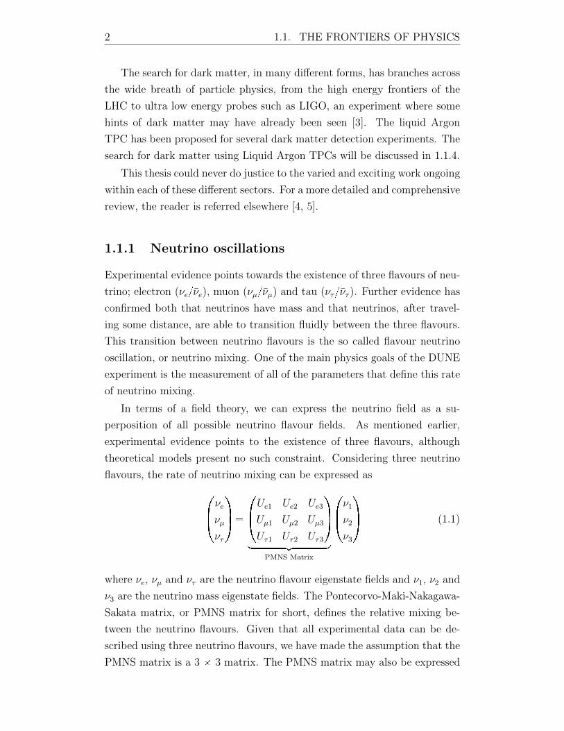
flavours, the rate of neutrino mixing can be expressed as
νe
νµ
ντ
Ue1 Ue2 Ue3
Uµ1 Uµ2 Uµ3
Uτ1 Uτ2 Uτ3
loooooooooomoooooooooonPMNS Matrix
ν1
ν2
ν3
(1.1)
where νe, νµ and ντ are the neutrino flavour eigenstate fields and ν1, ν2 and
ν3 are the neutrino mass eigenstate fields. The Pontecorvo-Maki-Nakagawa-
Sakata matrix, or PMNS matrix for short, defines the relative mixing be-
tween the neutrino flavours. Given that all experimental data can be de-
scribed using three neutrino flavours, we have made the assumption that the
PMNS matrix is a 3 3 matrix. The PMNS matrix may also be expressed
1.1. THE FRONTIERS OF PHYSICS 3
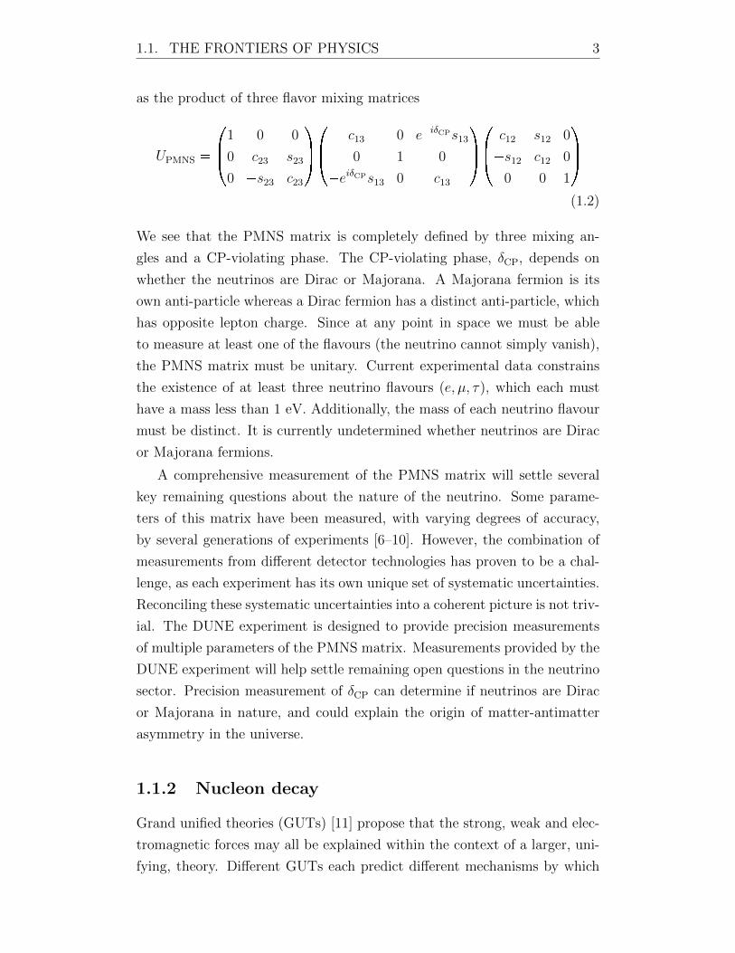
as the product of three flavor mixing matrices
UPMNS
1 0 0
0 c23 s23
0 s23 c23
c13 0 eiδCPs13
0 1 0
eiδCPs13 0 c13
c12 s12 0
s12 c12 0
0 0 1
(1.2)
We see that the PMNS matrix is completely defined by three mixing an-
gles and a CP-violating phase. The CP-violating phase, δCP, depends on
whether the neutrinos are Dirac or Majorana. A Majorana fermion is its
own anti-particle whereas a Dirac fermion has a distinct anti-particle, which
has opposite lepton charge. Since at any point in space we must be able
to measure at least one of the flavours (the neutrino cannot simply vanish),
the PMNS matrix must be unitary. Current experimental data constrains
the existence of at least three neutrino flavours (e, µ, τ), which each must
have a mass less than 1 eV. Additionally, the mass of each neutrino flavour
must be distinct. It is currently undetermined whether neutrinos are Dirac
or Majorana fermions.
A comprehensive measurement of the PMNS matrix will settle several
key remaining questions about the nature of the neutrino. Some parame-
ters of this matrix have been measured, with varying degrees of accuracy,
by several generations of experiments [6–10]. However, the combination of
measurements from different detector technologies has proven to be a chal-
lenge, as each experiment has its own unique set of systematic uncertainties.
Reconciling these systematic uncertainties into a coherent picture is not triv-
ial. The DUNE experiment is designed to provide precision measurements
of multiple parameters of the PMNS matrix. Measurements provided by the
DUNE experiment will help settle remaining open questions in the neutrino
sector. Precision measurement of δCP can determine if neutrinos are Dirac
or Majorana in nature, and could explain the origin of matter-antimatter
asymmetry in the universe.
1.1.2 Nucleon decay
Grand unified theories (GUTs) [11] propose that the strong, weak and elec-
tromagnetic forces may all be explained within the context of a larger, uni-
fying, theory. Different GUTs each predict different mechanisms by which
4 1.1. THE FRONTIERS OF PHYSICS
different nucleons may decay, and make predictions about the expected life-
time of the nucleon states. By searching for nucleon decays, or by setting
constraints on their lifetime by their absence, constraints can be set on al-
lowable GUTs. These constraints, if strict enough, may be incompatible
with certain theoretical models, ruling them out. An interesting specific
example is proton decay. In the standard model, proton decay is forbidden.
Hence, experimental observation of proton decay would be a clear sign of
physics beyond the standard model. Certain GUT models require proton
decay. For example, the Georgi–Glashow model requires that the proton
decays into a positron and neutral pion [12]. The neutral pion then decays
to two gammas. The half life for this decay is approximately 1034 years.
A natural byproduct of a 40-kiloton scale LArTPC is a large number of
nucleons contained within the detector. It is expected that the DUNE exper-
iment will extend the nucleon decay lifetime limits by an order of magnitude
beyond the current limits, set by Super-K, in several channels [1, 12]. Other
decay channels, however, remain better suited to large water Cherenkov de-
tectors due to differences in detector efficiencies. The searches performed
by the DUNE experiment are expected to be complimentary to those that
are proposed by Hyper-Kamiokande. A LArTPC has good efficiency for de-
tecting charged particles in the final state. Neutron decays are not detected
with good efficiency in a LArTPC due to the lack of charged particles in the
final state, thus producing no ionisation. Of particular interest are nucleon
decays which have a charged Kaon in the final state. Charged Kaons can
be detected with high efficiency in a LArTPC, since the high Kaon mass
results in a large ionisation yield. The relatively short lifetime of the Kaon
means that the decay products can also be detected in the LArTPC, in total
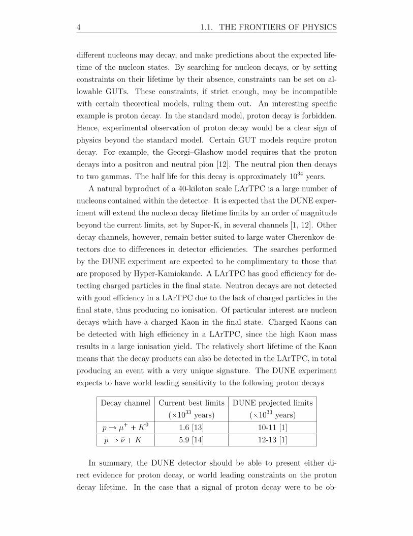
producing an event with a very unique signature. The DUNE experiment
expects to have world leading sensitivity to the following proton decays
Decay channel Current best limits DUNE projected limits
(1033 years) (1033 years)
pÑ µ K0 1.6 [13] 10-11 [1]
pÑ ν K 5.9 [14] 12-13 [1]
In summary, the DUNE detector should be able to present either di-
rect evidence for proton decay, or world leading constraints on the proton
decay lifetime. In the case that a signal of proton decay were to be ob-
1.1. THE FRONTIERS OF PHYSICS 5
served in DUNE, it would be important for the signal to also be observed in
Hyper-Kamiokande, given the different detection technologies. Complimen-
tary searches using multiple detection techniques can only be beneficial.
1.1.3 Supernovae
The neutrino flux that emanates from the core of a collapsing star gives a
unique insight into the physics that is ongoing during the supernovae. Ob-
servation of such a supernovae using the next generation of 40-kiloton scale
detectors would help to constrain the physical processes that are occurring
during core collapse. Both the flavour content and the flux of the neutrinos
which are emitted from a supernova vary over time through the different
stages of core collapse. Accurate measurement of these parameters through-
out the process of a supernovae will provide much needed constraints for
theoretical models [12].
The large number of neutrinos produced in supernovae present several
unique experimental opportunities. The quantity of neutrinos produced is
so large that neutrino-neutrino coherent scattering is expected to be a mea-
surable effect. Supernovae present the only experimental opportunity to
measure this effect. The large distance traveled by supernova neutrinos
before reaching earth also provides an uniquely long baseline for time-of-
flight measurements. These time-of-flight measurements provide a way to
search for Lorentz and CPT-violating effects in neutrinos. These effects are
quantised using standard model extension parameters (SMEs) [15]. For a
supernova comparable to SN1987, at a distance of 50 kpc, Figure 1.1 sum-
marises the projected improvements to the SME parameters that could be
provided by DUNE.
1.1.4 Dark matter searches using Liquid Argon
Several experiments have proposed the use of Liquid Argon TPCs for dark
matter detection attempts. DarkSide-20k [16] is a proposed 20 Tonne Two-
Phase LAr TPC for direct dark matter detection. ArDM [17–19] is a ton-
scale Liquid Argon TPC for direct dark matter searches whilst WArP [20]
has a sensitive mass of 140 kg Argon.
Many of these dark matter searches using LArTPCs feature similar de-
tector configurations; A sensitive volume which is surrounded by a large
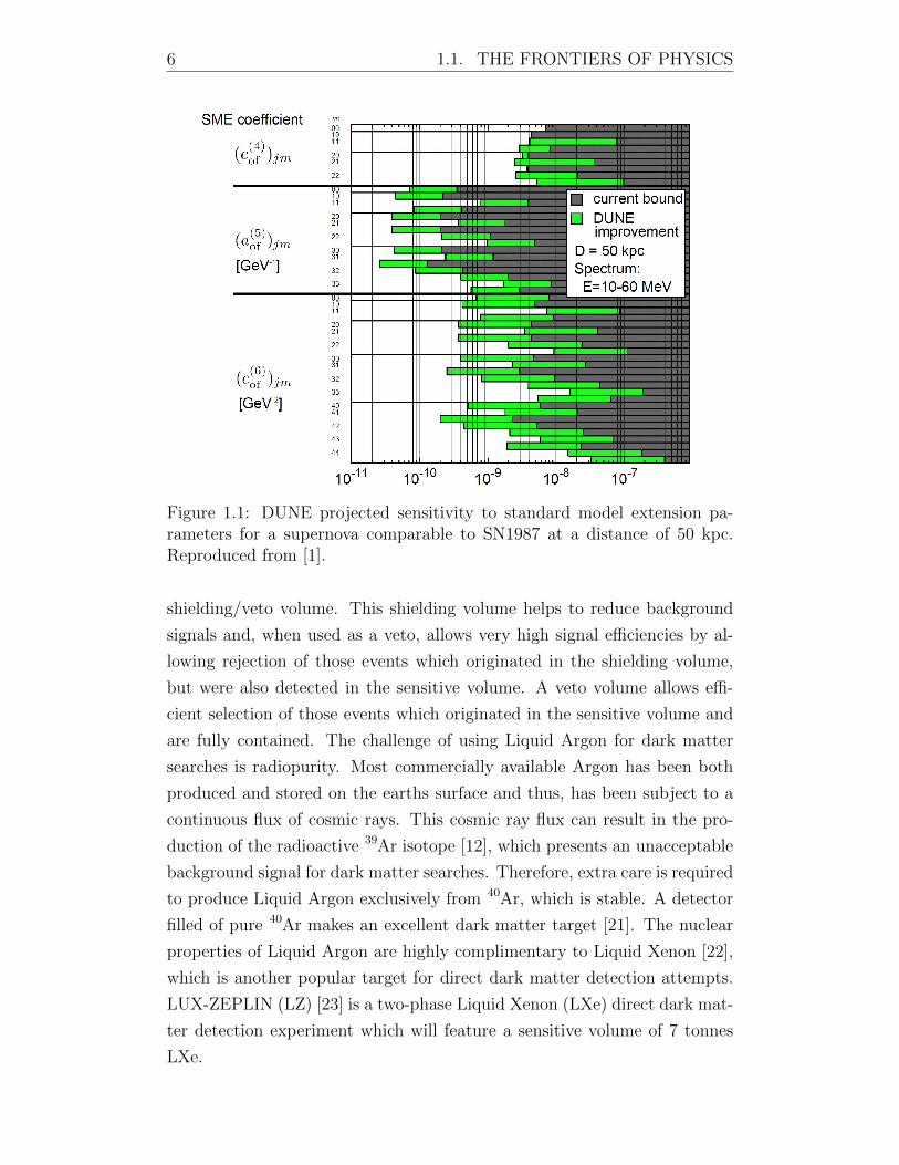
6 1.1. THE FRONTIERS OF PHYSICS
Figure 1.1: DUNE projected sensitivity to standard model extension pa-rameters for a supernova comparable to SN1987 at a distance of 50 kpc.Reproduced from [1].
shielding/veto volume. This shielding volume helps to reduce background
signals and, when used as a veto, allows very high signal efficiencies by al-
lowing rejection of those events which originated in the shielding volume,
but were also detected in the sensitive volume. A veto volume allows effi-
cient selection of those events which originated in the sensitive volume and
are fully contained. The challenge of using Liquid Argon for dark matter
searches is radiopurity. Most commercially available Argon has been both
produced and stored on the earths surface and thus, has been subject to a
continuous flux of cosmic rays. This cosmic ray flux can result in the pro-
duction of the radioactive 39Ar isotope [12], which presents an unacceptable
background signal for dark matter searches. Therefore, extra care is required
to produce Liquid Argon exclusively from 40Ar, which is stable. A detector
filled of pure 40Ar makes an excellent dark matter target [21]. The nuclear
properties of Liquid Argon are highly complimentary to Liquid Xenon [22],
which is another popular target for direct dark matter detection attempts.
LUX-ZEPLIN (LZ) [23] is a two-phase Liquid Xenon (LXe) direct dark mat-
ter detection experiment which will feature a sensitive volume of 7 tonnes
LXe.
Chapter 2
The Liquid Argon time
projection chamber
2.1 Liquid Argon as a detector target
As described by Carlo Rubbia in 1977 [24], several properties make Liquid
Argon a good target for particle detection. Liquid Argon is dense, encour-
aging interactions. Liquid Argon has high electron mobility and does not
capture drifting electrons. Both of these features allow for efficient drift over
long distances. Crucially, Liquid Argon is cheap. The realisation of future
experiments with sensitive volumes in the region of 40 kiloton is sensitively
dependent on the cost of the chosen target material. The favorable elec-
tron transport characteristics of Liquid Argon are only true for highly pure
Liquid Argon. Small levels of impurities can destroy these important char-
acteristics. Purification of Liquid Argon remains a considerable challenge
for current Liquid Argon TPC based experiments. Liquid Argon produces
copious amounts of scintillation light (few tens of thousands of photons per
MeV [25]) and is transparent to this scintillation light, allowing for efficient
detection.
However, Liquid Argon has some considerable drawbacks. The cryogenic
nature of Liquid Argon requires the construction and use of cryostats, which
become costly for large experiments. The requirement that detector com-
ponents should be able to operate for long periods of times in cryogenic
conditions gives rise to engineering challenges. The most abundant, and
therefore cheapest, form of Argon is 40Ar. When exposed to cosmic rays,39Ar may be produced [26]. 39Ar is radioactive, making its presence largely
7
8 2.1. LIQUID ARGON AS A DETECTOR TARGET
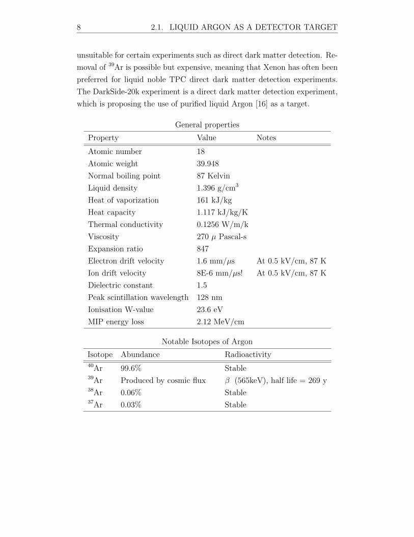
unsuitable for certain experiments such as direct dark matter detection. Re-
moval of 39Ar is possible but expensive, meaning that Xenon has often been
preferred for liquid noble TPC direct dark matter detection experiments.
The DarkSide-20k experiment is a direct dark matter detection experiment,
which is proposing the use of purified liquid Argon [16] as a target.
General properties
Property Value Notes
Atomic number 18
Atomic weight 39.948
Normal boiling point 87 Kelvin
Liquid density 1.396 g/cm3
Heat of vaporization 161 kJ/kg
Heat capacity 1.117 kJ/kg/K
Thermal conductivity 0.1256 W/m/k
Viscosity 270 µ Pascal-s
Expansion ratio 847
Electron drift velocity 1.6 mm/µs At 0.5 kV/cm, 87 K
Ion drift velocity 8E-6 mm/µs! At 0.5 kV/cm, 87 K
Dielectric constant 1.5
Peak scintillation wavelength 128 nm
Ionisation W-value 23.6 eV
MIP energy loss 2.12 MeV/cm
Notable Isotopes of Argon
Isotope Abundance Radioactivity40Ar 99.6% Stable39Ar Produced by cosmic flux β(565keV), half life = 269 y38Ar 0.06% Stable37Ar 0.03% Stable
2.2. INTERACTIONS OF PARTICLES WITH MATTER 9
2.2 Interactions of particles with matter
2.2.1 Relativistic charged particles
A complete review of the interactions of particles with matter is given in [5].
Here we will instead discuss aspects that are directly relevant in the context
of a Liquid Argon TPC. When a charged particle traverses through Liquid
Argon, a mixture of ionisation and excitation is produced, generally by suc-
cessive single collisions with electrons of the Argon atoms. The energy loss
of the charged particle is often quoted as dEdX. The ”Bethe equation” is
the most widely used theoretical model to predict energy loss for relativistic
heavy charged particles. This model predicts, with accuracy within a few
percent, the mean energy loss for particles in the region 0.1 ¤ βγ ¤1000 for
most materials with Z ¡ 10. The ”Bethe equation” is as follows:
x dEdX
y Kz2Z
A
1
β2
1
2ln
2mec2β2γ2Wmax
I2 β2 δpβγq2
(2.1)
where xdEdXy is the mean energy loss. K 4πNAre2mec
2, where NA
is Avogadro’s number, re is the classical electron radius, me is the electron
mass and c is the speed of light. ze is the charge of the incident particle. Z is
the absorber atomic number. Wmax is the maximum kinetic energy transfer
in a single collision with a single electron and I is the mean excitation energy.
δpβγq is the density-effect correction [27].
Let us consider the case of many cosmic muons passing through a LArTPC.
The distribution of energy lost by these muons can be approximately de-
scribed using a Landau distribution. This distribution has a peak at the
so called ’most probable value’ followed by an extensive tail out to higher
energies. This long tail is the result of the rarer collision processes. It is
this tail that means xdEdXy must be used with caution. The mean of
the energy loss distribution is heavily weighted by this tail, the tail which is
formed from rare processes that may not well represented, even with mod-
est number of events. It is for this reason that the most probable value of
a Landau fit is instead generally a more robust measure of energy loss. The
peak of the most probably energy loss is formed much more reliably by the
abundant lower energy collisions.
Occasionally, it is possible that a very large momentum transfer occurs
to a single electron. This single electron gains so much kinetic energy that it
10 2.2. INTERACTIONS OF PARTICLES WITH MATTER
itself can become ionising and produce an observable track in the detector.
This track is known as a delta ray (δ-ray) and can be seen as small branches
from tracks which are otherwise expected to be only ionising.
Event reconstruction and analysis techniques can often exacerbate the
difficulties with using the mean energy loss as a tool for particle identifica-
tion. In order for the mean energy loss to represent a reliable measure, the
analysis method must be able to reliably reconstruct the additional energy
loss contained within δ-rays, and reliably associate this energy loss to the
parent track.
2.2.2 Multiple Coulomb scattering (MCS)
As well as losing energy, particles are also scattered during their traversal
of matter. The distribution of scattering angles is expected to be mostly
Gaussian but once again a large tail may exist as a result of rarer scattering
events that can produce large angles, for example nuclear recoils. The stan-
dard deviation of the scattering distribution is predicted by Lynch & Dahl
[28] as:
θ0 13.6 MeV
βcpz
cx
X0
1 0.038 lnp x
X0
q
(2.2)
Where p is the particle momentum, βc is the particle velocity and z is
the charge number of the incoming particle. xX0 is the thickness of the
scattering medium with units of radiation lengths.
Energy reconstruction of particles in the LArTPC is perhaps better
known using energy loss, or dEdX. Measurements of multiple coulomb
scattering however give an additional handle on the momenta of a particle
in a TPC and are undoubtedly useful. Both ICARUS and Microboone have
recently been exploring this concept [29, 30].
Multiple Coulomb scattering (MCS) should be considered as a compli-
mentary handle on particle momentum compared to dEdX. Reconstruction
of particle momenta through either dEdX or MCS can excel under differ-
ent circumstances. In the case that Liquid Argon purity is poor, ionisation
electrons may be lost during the drift. In the case of an analysis which solely
uses dEdX, care must be taken to ensure that either the Liquid argon pu-
rity is so great that electron capture by impurities is not an issue or that
accurate purity corrections are performed. Using MCS to determine particle
2.2. INTERACTIONS OF PARTICLES WITH MATTER 11
momenta is generally insensitive to purity effects since, even if a track has
extreme variations in relative intensity throughout it’s length by impurity
attachment, this will have little effect on the resolved track position. On the
other hand, in the case of a TPC which has high field non-uniformities, accu-
rate measurement of MCS may be a challenge. Drift field non-uniformities
will distort the reconstructed position of the track in the TPC and lead
to unreliable MCS measurements. In this case, momentum measurement
via dEdX may be more reliable. In any real TPC, there is most likely
a combination of both purity effects and drift field non-uniformities and
so complimentary MCS and dEdX momentum measurements should be
considered.
12 2.3. IONISATION
2.3 Ionisation
As a charged particle traverses Liqud Argon, Argon atoms may be ionised.
The energy required to liberate an electron from an Argon atom is known
as the W-value. The W-value for Liquid Argon has been measured as
23.60.50.3 eV [31]. For reference, the W-value for gas Argon has been measured
as 26.30.2 eV [32].
We can use the W-value to predict the number of electrons that will be
liberated by an ionising particle in the LArTPC. Naturally, the number of
liberated electrons is not exact, but is according to a roughly Gaussian dis-
tribution. The standard deviation of this distribution is predicted according
to?FN , where F is the so called Fano-factor and N is the mean number
of created electron-ion pairs. The Fano-factor has been calculated to be in
the range 0.107-0.116 for Liquid Argon [33].
We can predict that, for a minimum ionising particle (MIP) with dEdX 2.12 MeV/cm, the mean ionisation yield is 89800 electron-ion pairs per cen-
timeter with a standard deviation of 9880. The Fano factor places a limit on
the energy resolution that is possible in an ionisation detector. If we assume
that F 0.11, the limiting energy resolution is given as roughly 0.33?N ,
where N is the number of electron-ion pairs. If we consider a 1 cm segment
of a MIP-like track, this limiting resolution is around 11%.
In practice, detector effects mean that this limiting resolution imposed
by the Fano-factor is never realised. Of all of the electron-ion pairs that
are initially created by an ionising event, a large fraction are lost almost
immediately to recombination. Even more electrons are lost by attachment
to impurities during drift. Both of these effects degrade energy resolution.
2.3.1 Recombination
The effect of electron recombination in Liquid Argon is often quoted as a
recombination factor, R. If we let the initial number of liberated electron-
ion pairs equal Q0 then R is defined as Q Q0R, where Q is the number of
electron-ion pairs which survive recombination. The rate of recombination
is generally assumed to be a function of ionisation density as well as the
applied electric field, ~E. In the limit of no electric field, all ionised charge
is expected to eventually recombine (lim ~EÑ0R 0). Conversely, in the
limit of infinite electric field, all charge is expected to survive recombination
2.3. IONISATION 13
(lim ~EÑ8R 1). The dependence of the rate of recombination on the ioni-
sation charge density is often parameterised using dEdX. However, since
ionisation charge density is not strictly proportional to dEdX, this depen-
dence should be considered as an approximation. In other words, the true
recombination rate is expected to vary depending on the type of ionising
particle, rather than simply dEdX.
The ICARUS collaboration, and later the ArgoNeuT collaboration, have
both performed detailed studies of the rate of recombination in Liquid Ar-
gon [34, 35]. These studies represent the most in-depth understanding of
recombination theory in Liquid Argon. The most important results from
both of these studies will be highlighted in the following discussion.
It is also worth noting that recombination and light production by scin-
tillation in Liquid Argon are closely related. We will see later that, as an end
result of the recombination process, scintillation light is produced. Thus, as
recombination is reduced, total scintillation output is also reduced.
Many theories of electron recombination have been proposed in the lit-
erature. The earliest models, the so called geminate theory [36], suggest
that each ion and electron pair should be considered independently. After
ionisation, the ion and electron both move under the effects of diffusion,
their mutual coulomb attraction and the forces applied by external electric
fields. The germinate model predicts that if recombination does happen, the
electron recombines with the exact ion from which it originated. This recom-
bination of the electron with its parent ion is known as initial recombination.
In order for this model to be realistic, it is obvious that the electron must
remain close to the ion from which it originated. If the electron escapes to a
distance far from the initial ion, there is no reason to expect for it to recom-
bine with the parent ion, and not another available ion nearby. Electrons,
once ionised, have a large amount of kinetic energy. Their high kinetic en-
ergy means that electrons are not immediately able to recombine, but must
first thermalise. The process of thermalisation happens very quickly, on the
order of nanoseconds [37, 38]. During this time, calculations and simula-
tions showed that the electrons will travel a mean thermalisation distance
of roughly 2.6 µm [38]. This thermalisation distance is much further than
the reasonable range of the attractive coloumb force between the parent ion
and the ionised electron (The average interatomic spacing is approximately
4A [39]). Thus, these considerations suggest that direct recombination with
14 2.3. IONISATION
the parent ion is unlikely. A critical test showed that, in Liquid Argon, data
does not agree well with germinate theory [40].
The elimination of germinate theory thus leads to the conclusion that
ionised electrons are instead mostly effected by the collective forces from
the total ion cloud around an ionising track. Columnar theory [41] predicts
that an ionising track creates a dense column of ions and electrons around
the core of the track. The core of the column is formed by the relatively
immobile ions and the periphery of the column is formed by a cylindrical
cloud of electrons. According to this model, the ions and electrons are to
drift away from the central core of the column as a result of diffusion and as
the result of any applied electric field. The predictions of columnar theory,
according to Jaffe’s model, can be expressed using a form of Birk’s law:
RJaffe 1
1 q0F p ~E sinφq (2.3)
where q0 is the initial ionisation density, ~E is the applied electric field, at
an angle φ relative to the ionisation column. F is a function which param-
eterises the diffusion of electrons and ions, dependent on the diffusion and
mobility coefficients in the Liquid Argon. A recent modification of Jaffe’s
theory is the so called ’modified columnar theory’ proposed by Kramers [42].
This model incorporates more realistic model of electron diffusion which has
a strong effect on the predictions of the model at low ionisation densities.
A shared limitation of both Jaffe’s and Kramers’ model is the assumption
that electrons and ions have equal drift velocities and that their mobility
is independent of the applied electric field. Both of these assumptions are
demonstrably false.
Thomas and Imel proposed a new model which reworks the assumptions
made by both Jaffe and Kramers [43]. This model instead assumes that ions
are immobile and there is zero diffusion. This model replaces the columnar
structure of the ionised charge cloud with a uniformly distributed box ge-
ometry. This model is therefore commonly known as the box model. This
model predicts that:
RBox 1
ξln p1 ξq, where ξ N0
4a2µ~E(2.4)
where N04a2 represents the charge density inside a microscopic box of side
2.3. IONISATION 15
length a. µ is the electron mobility and ~E is the applied electric field.
A limitation of both the columnar and box theories is that they all as-
sume that the electron drift velocity is linearly proportional to the applied
electric field. In the case of Liquid Argon, this assumption is incorrect above
0.2 kV/cm [44], far below the nominal drift field of most experiments. Ad-
ditionally, the box model includes no dependence on the track angle relative
to the electric field direction. Although these limitation are fundamental,
both models are still able to provide reasonable agreement with experimental
data, albeit in limited regimes.
Electron recombination in Liquid Argon is still an active area of research.
We have discussed the two most widespread theories, the box model and
the modified columnar model. These models each only provide reasonable
agreement with experimental data over a subset of electric field values. So
far, the most accepted model appears to be an approximate solution to
Equation 2.4, given by a form of Birk’s law:
RBox 1
1 keξ(2.5)
where ke is left as a constant, to be determined by fitting to experimental
data. The ICARUS collaboration found that an additional scaling factor,
A, substantially improves the fit of the model to the data and so we finally
reach
RBox A
1 keξ(2.6)
where both A and ke are determined by fitting. Looking back at Equation
2.4, ξ is seen to be a function of the initial ionised charge density, electron
mobility and applied electric field. Given that relatively little data exists
about the ionisation charge density as a function of energy for many particle
types, an approximation is generally made that the ionisation charge den-
sity is proportional to dEdX. Thus, the term N04a2 can be re-expressed
as k dEdX. We now reach a final expression for electron recombination
as a function of dEdX and electric field ~E, parameters which are easily
measured in a LArTPC:
RBox A
1 kqdEdX
~E
(2.7)
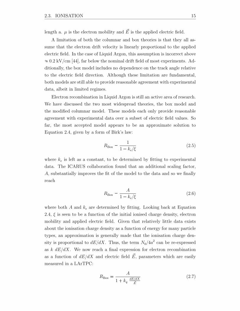
16 2.3. IONISATION
5 10 15 20 25 30linear stopping power [dE/dX]
0
0.1
0.2
0.3
0.4
0.5
0.6
0.7
0.8
0.9
1
Rec
ombi
natio
n fa
ctor
, R
ICARUS 3t, Nucl. Instr. Meth, vol. A523 (2004)
ArgoNeuT, JINST 8 P08005 (2013)
ICARUS T600, Nucl. Instr. Meth, vol. A523 (2004)
Figure 2.1: Experimental measurements of the recombination factor as afunction of stopping power. The best model constraints are provided byICARUS T600 [34]. The functional form of the model is described in Equa-tion 2.7. The model of valid for drift fields between 0.1-1.0 kV/cm, whichprovides comprehensive coverage across most drift fields typically used inmost experiments. This model is valid for protons and muons with dEdXin the range 1.5 to 30 MeV/(g/cm2).
According to ICARUS [34], the experimental values for the parametersA and
kq are given byA 0.8000.003 and kq 0.04860.0006 (kV/cm)(g/cm2)/MeV.
These values are valid for electric fields between 0.1 and 1.0 kV/cm and
for dEdX between 1.5 to 30 MeV/(g/cm2). These values have been in-
dependently verified by the ArgoNeuT collaboration [35] who found that
A 0.793 0.018 and kq 0.049 0.002 (kV/cm)(g/cm2)/MeV. The
predictions of Equation 2.7 are plotted as a function of dEdX in Figure
2.1 for a fixed electric field of 0.5 kV/cm. The predictions are plotted for
three different versions of the parameters A and B, from the results of three
different detectors. The tightest predictions are from the ICARUS T600
detector. The fit parameters from ICARUS 3t and ArgoNeuT are constant
with the parameters found by ICARUS T600 but both have relatively larger
uncertainties.
2.4. SCINTILLATION 17
2.4 Scintillation
When charged particles interact with Liquid Argon, a mixture of both ioni-
sation and excitation of Argon atoms occurs. Both the ionisation and exci-
tation phenomena can eventually lead to the emission of scintillation light.
In the case of Argon excitation, an excited Ar state is produced. The de-
excitation process for Ar, and other noble gasses, is more involved than a
direct de-excitation with the emission of a photon. Argon, like other no-
ble gasses, has a full outer shell. This full outer shell means that covalent
bonding is minimal between neighbouring Argon atoms, when in the ground
state. However, when an Argon atom is excited, the electron leaves behind
a hole in the valence shell, meaning that covalent bonding may now be pos-
sible. Figure 2.3 plots the potential curves for excited Argon atoms as a
function of nuclear separation. We see that the potential for excited Ar
states features a dip in potential if an excited Ar state moves closer to a
ground state Ar atom, forming a covalent bond. The resulting molecule,
formed from a ground state Ar Atom and an excited Ar atom, is known as
an excimer. This excimer state may be expressed as pArArq. The emission
spectrum of Argon is defined by all the possible ways by which this excimer
can decay back into the ground state.
In Argon, there are two possible excimer states than can be formed,
seen as the red and blue potentials on Figure 2.3. The difference between
these two states is related to the spin of the excited electron. Since Argon
has a closed shell structure, in the ground state all electrons are paired, Ö.
When one of these electrons is excited, the spin of the excited electron may
stay paired with the ground state electron, giving for example spin-Ò in the
ground state and spin-Ó in the excited state. In the case that the spins
remain coupled in this way, the excited state is known as the singlet excited
state. It is also possible that the spin of the excited electron can decouple
from the spin of the ground state electron. In this case we could have, for
example, spin-Ò in the ground state and also spin-Ò in the excited state. A
state in which the spin of the excited electron aligns with the spin of the
ground state electron is known as the triplet excited state. On Figure 2.3,
we see the singlet state as 1Σu (red line) and the triplet state as 3Σ
u (blue
line). The decay of both the singlet and triplet states to the ground state 1Σg
(black line) is mediated by the emission of a VUV photon. The wavelength
18 2.4. SCINTILLATION
Ar
Ar Ar*
Ar
Ar
Ar
Ar*
Ar*
Ar*
Ar+
Ar+
Ar+
Ar+
e-
e-
e-
e-
Ar*
Ar*Ar
(ArAr)*
Excimer formation
ArAr
(ArAr)* Excimer de-excitesby emission of a VUV photon
127nm
Ar Ar+
(ArAr)+ self trapped hole formation
Ar Ar+
Recombinatione-
Ar Ar**
(ArAr)+ recombines toAr + Ar**
Ar**Ar
(ArAr)**
Excimer formation
Ar*Ar
(ArAr)** Relaxes to(ArAr)* non-radiatively
Ar
Self-trapped exciton luminescence
Recombinationluminescence
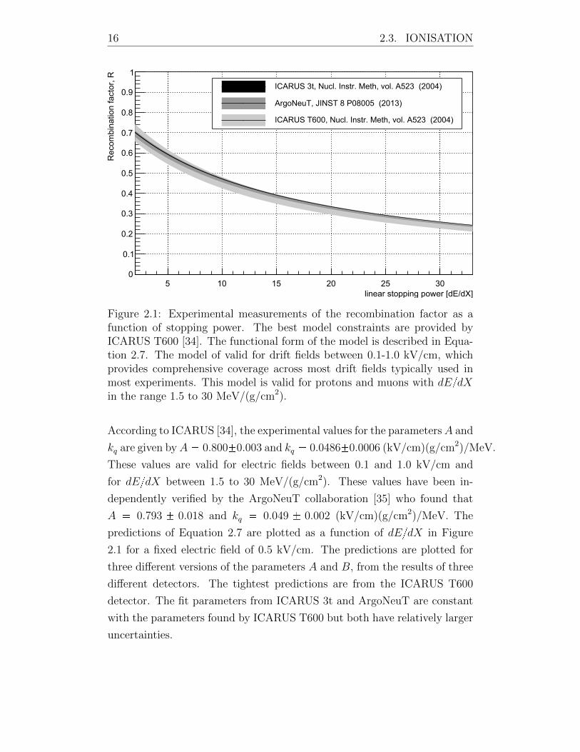
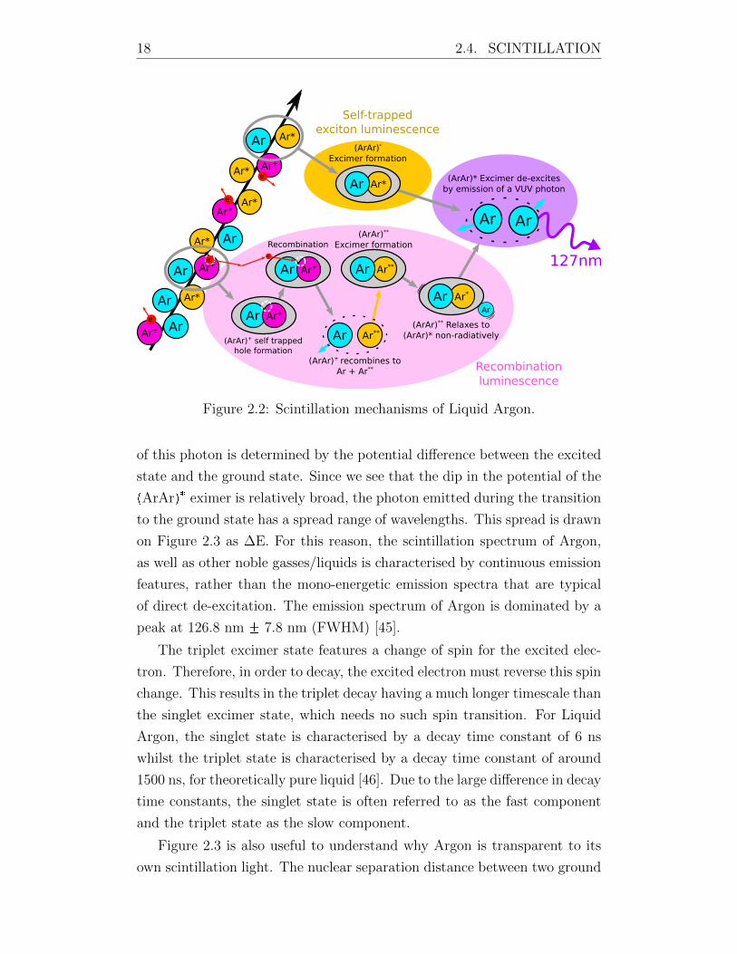
Figure 2.2: Scintillation mechanisms of Liquid Argon.
of this photon is determined by the potential difference between the excited
state and the ground state. Since we see that the dip in the potential of the
pArArq eximer is relatively broad, the photon emitted during the transition
to the ground state has a spread range of wavelengths. This spread is drawn
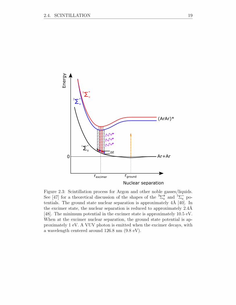
on Figure 2.3 as ∆E. For this reason, the scintillation spectrum of Argon,
as well as other noble gasses/liquids is characterised by continuous emission
features, rather than the mono-energetic emission spectra that are typical
of direct de-excitation. The emission spectrum of Argon is dominated by a
peak at 126.8 nm 7.8 nm (FWHM) [45].
The triplet excimer state features a change of spin for the excited elec-
tron. Therefore, in order to decay, the excited electron must reverse this spin
change. This results in the triplet decay having a much longer timescale than
the singlet excimer state, which needs no such spin transition. For Liquid
Argon, the singlet state is characterised by a decay time constant of 6 ns
whilst the triplet state is characterised by a decay time constant of around
1500 ns, for theoretically pure liquid [46]. Due to the large difference in decay
time constants, the singlet state is often referred to as the fast component
and the triplet state as the slow component.
Figure 2.3 is also useful to understand why Argon is transparent to its
own scintillation light. The nuclear separation distance between two ground
2.4. SCINTILLATION 19
Ener
gy
Nuclear separation
0 Ar+Ar
(ArAr)*
Σ+
u
1
Σ+
u
3
Σ+
g
1
rgroundrexcimer
ΔE
Figure 2.3: Scintillation process for Argon and other noble gasses/liquids.See [47] for a theoretical discussion of the shapes of the 3Σ
u and 1Σu po-
tentials. The ground state nuclear separation is approximately 4A [40]. Inthe excimer state, the nuclear separation is reduced to approximately 2.4A[48]. The minimum potential in the excimer state is approximately 10.5 eV.When at the excimer nuclear separation, the ground state potential is ap-proximately 1 eV. A VUV photon is emitted when the excimer decays, witha wavelength centered around 126.8 nm (9.8 eV).
20 2.4. SCINTILLATION
state Argon atoms is much larger than that of Argon excimers, labeled on
Figure 2.3 as rground and rexcimer respectively. The difference in potential
between both the 3Σu and 1Σ
u states to the ground state 1Σg at rexcimer is
much smaller than at rground. Thus, it can be seen that the energy carried by
the decay of the excimer is not sufficient to excite two ground state Argon
atoms back to an pArArq excimer (orange arrow).
Now that we understand how pArArq excimers produce scintillation light
in Argon, we must consider the possible ways that pArArq eximers can be
produced. The most straightforward method is the excitation of Argon
atoms by charged particle passage. These excited Ar atoms immediately
go on to form the pArArq eximers, then decay to produce scintillation light.
However, charged particle passage through Argon can also cause ionisation.
The ionisation process creates Argon ions, Ar and free electrons. Analo-
gous to the formation of the pArArq excimers, the newly created hole of the
Ar ion makes it is energetically favourable to form a bond with a nearby
ground state Argon atom [49]. The resulting molecule, pArArq, contains
what is known as a self-trapped hole. If an electron is able to re-combine
with this trapped hole, the two neutral Argon atoms can be reformed. Once
an electron is recombined with the self-trapped hole, it is no longer en-
ergetically favourable for the pArArq molecule to exist. Thus, the two
Argon atoms rapidly repel each other and disassociate. When the pArArqmolecule dissociates to re-form the two neutral Argon atoms, one of these
atoms is produced in a highly excited state, Ar. Once again, it is energeti-
cally favourable for this highly excited Ar atom to associate with a nearby
Argon atom, forming the pArArq molecule. This pArArq molecule un-
dergoes a dissociation to lower excited Ar state plus a ground state Argon
atom [50, 51], possibly by a phonon induced radiationless transition [52].
Little or no experimental data is available on this process of dissociation
and the mechanism is not well understood. The remaining Ar is able to,
as before, form an pArArq excimer and finally dissociate to ground state
Ar Ar by the emission of a VUV photon. Figure 2.2 illustrates these
scintillation processes.
Although Argon predominantly scintillates at 126.8 nm, a modest quan-
tity of photons are also generated in the near-infrared (NIR), peaking at
970 nm [45, 53, 54]. The electroluminescence yield of the NIR component of
Argon has been measured elsewhere to be approximately six times less than
2.4. SCINTILLATION 21
the VUV component [54]. The detection of these NIR photons may be more
straightforward than detection of the VUV component, since wavelength
shifting can be avoided.
2.4.1 Quenching of scintillation light by impurities
We saw in Section 2.4 that, in Argon, scintillation light production is the
result of radiative de-excitation of the pArArq excimer. The emission of
the VUV photon from either the singlet or triplet excimer state takes some
time, characterised by the time constants of each process. In the case of
the singlet, the time constant is τ1 = 2-6 ns. For the triplet state, the time
constant is τ2 1500 ns for perfectly pure liquid Argon.
For the excimer state to radiatively decay with the emission of a VUV
photon, the excimer state must exist long enough for the process to oc-
cur. In other words, if some other process causes the excimer to de-excite
non-radiatively, the emission of a VUV photon no longer occurs. It is pos-
sible that, in the presence of impurities, other processes can cause the non-
radiative de-excitation of the excimer. Of particular significance is the colli-
sional de-excitaiton of the excimer to ground state. In the presence of impu-
rities, pArArq can undergo a two-body collision, pArArq X Ñ 2 ArX,
where X is the impurity atom/molecule. This collisional de-excitaiton pro-
cess is non-radiative, and thus the excimer no longer produces a VUV pho-
ton. This reduction in scintillation light production is known as quenching.
Given the longer decay time constant of the triplet state, it is intuitive
that the triplet state is more sensitive to the presence of impurities than the
singlet state. Simply put, the triplet state exists for a longer time and there-
fore has an increased time window to collide with impurity atoms/molecules
and be de-excited collisionally. For the impurity concentrations typical in
LArTPCs, the very short decay time of the singlet state makes it relatively
insensitive to impurity concentration. Many studies have been performed
in the literature to quantify the quenching of Argon scintillation by differ-
ent impurities, X. Particular interest has been paid to those impurities
which are typically found in commercial Liquid and gas Argon. High pu-
rity commercial Liquid Argon typically contains trace quantities of Oxygen,
Water, Carbon monoxide, Hydrogen and other hydrocarbons, each at the
¤ 1 ppm level. Liquid Argon also typically contains trace Nitrogen at a
higher level, typically ¤ 3 ppm. Carbon Dioxide is present a lower level, typ-
22 2.4. SCINTILLATION
ically ¤ 0.5 ppm. The effects of Oxygen and Nitrogen are well represented in
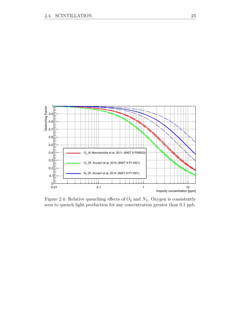
the literature for liquid Argon [55–57]. Figure 2.4 plots the quenching factor
for Oxygen and Nitrogen as a function of impurity concentration. The effects
of Carbon monoxide and Hydrogen appear to have not been studied, despite
their typical presence in N6.0 liquid Argon. Of all the hydrocarbons, only
Methane appears to have been studied in any detail [58], yet was shown to
have a substantial quenching effect, reaching a quenching factor of roughly
0.8 at only 0.1 ppm impurity. This quenching effect of Methane appears to
be the strongest of all of the tested impurities. Given that commercial liquid
Argon typically contains 1 ppm of trade hydrocarbons, it would seem that
purification/filtration of Methane should be given some consideration.
The quenching effect of H2O, and CO2 have been measured in gas Argon
[55] and show quenching effects similar to that of O2. Nitrogen is consistently
seen to quench scintillation light at a slower rate than other impurities.
Both H2O and O2 are extensively purified in Liquid Argon TPCs for reasons
other than scintillation light production (See Section 2.5.3). The removal of
H2O and O2 is typically so effective that they should have essentially zero
impact on scintillation light production. Filtration of Nitrogen and other
proven quenchers is typically not performed. Perhaps an improvement of
scintillation light production may be possible if the filtration of Nitrogen,
and possibly Methane and other unknown hydrocarbons, is considered.
2.4. SCINTILLATION 23
0.01 0.1 1 10Impurity concentration [ppm]
0
0.1
0.2
0.3
0.4
0.5
0.6
0.7
0.8
0.9
1
Que
nchi
ng F
acto
r
(K Mavrokoridis et al, 2011 JINST 6 P08003)2
O
(R. Acciarri et al, 2014 JINST 9 P11001)2
O
(R. Acciarri et al, 2014 JINST 9 P11001)2N
Figure 2.4: Relative quenching effects of O2 and N2. Oxygen is consistentlyseen to quench light production for any concentration greater than 0.1 ppb.
24 2.5. ELECTRON TRANSPORT
2.5 Electron transport
In order to operate as a TPC, the ionised charge must be collected. An
externally applied electric field induces the net motion of the ionised elec-
trons, typically directing them towards a readout device. This net motion of
electrons in the Liquid Argon is called drift. As we saw in Section 2.3.1, the
fraction of electrons that survive recombination, and thus are detectable, is
dependent on the magnitude of the electric field. For a MIP, at 0.5 kV/cm,
the recombination factor is approximately 0.7. This means that approxi-
mately 70 % of electrons are available for detection, whilst 30 % recombine.
The nature of a TPC is that the z dimension (the direction along the drift) is
not explicitly detected. The z position is instead inferred, assuming a known
drift velocity of the electrons in the TPC. This assumption of course requires
that the drift velocity be known precisely for best possible resolution in z.
In general, the collective motion of a charge cloud in Liquid Argon can
be described by the combination of several effects. First, there may be a
net motion of the charge cloud as the result of an applied electric field.
Secondly, over time, the charge cloud can diffuse and grow in space. Finally,
the total number of electrons in the charge cloud can change. Attachment
of the electrons to electronegative impurities causes the net reduction in the
number of electrons. At very high electric fields, ionisation could cause an
increase in the net number of electrons in the charge cloud. Ionisation is not
present at the drift fields typical used and so in general the net number of
electrons in the charge cloud tends only to decrease during the drift. These
collective effects may be described using Fick’s equation [59, 60]. Let n
describe the development of the charge cloud in px, y, z, tq. The drift field
is applied in the z direction. Under these circumstances, Fick’s equation
can be expressed as:
BnBt DL
B2n
Bz2 DT
B2n
Bx2 B2n
By2
v
B2n
Bz λvn (2.8)
The coefficients DL and DT parameterise the rate of diffusion in the lon-
gitudinal and transverse planes, respectively. The negative sign in front of
the vB2nBz term is explained by the fact that electrons drift in the oppo-
site direction of the drift field. In other words, the net motion of electrons
is backwards along the field lines of the drift field. Since we assumed the
2.5. ELECTRON TRANSPORT 25
drift field was applied in the z direction, the net motion of the charge
cloud is in the z direction. λ parameterises the loss or gain of electrons
by impurity attachment or ionisation. As mentioned earlier, λ almost ex-
clusively describes losses by attachment to impurities. The general solution
to Equation 2.8 is given by:
n n0
4πDT t?
4πDLtexp
pz vtq2
4DLt
loooooooooomoooooooooon
Longitudinaldiffusion
exp
x2 y2
4DT t
loooooooomoooooooon
Transversediffusion
exp pλvtqlooooomooooonImpurity
attachment
(2.9)
where n0 is the number of electrons at px, y, zq p0, 0, 0q at t 0. This
solution neatly decomposes into three distinct exponentials. Models for both
longitudinal and transverse diffusion are discussed in Section 2.5.2. Models
for the drift velocity, v, are discussed in Section 2.5.1. Finally, a discussion
of λ, the attachment of electrons to impurities, is given in Section 2.5.3.
2.5.1 Electron drift velocity
In 2000, W. Walkowiak studied the drift velocity of electrons in Liquid Argon
over a large range of drift fields (0.5 kV/cm - 12.6 kV/cm) [61]. Given that
0.5 kV/cm is the nominal operating field of many experiments, the lower
limit of the work performed by W. Walkowiak was not ideal. In 2004, the
ICARUS collaboration performed a study, extending the measurements of
electron drift velocity to a range more suitable to LArTPCs (0.056 kV/cm -
1 kV/cm) [62]. This study found results that were in good agreement with
the model proposed by W. Walkowiak, in the range that Walkowiak origi-
nally proposed. Below to 0.5 kV/cm the measured drift velocities began to
diverge from the predictions of the model. Considering the lower limit that
W. Walkowiak proposed of 0.5 kV/cm, this is perhaps unsurprising. The
ICARUS study did not propose any new function to describe their experi-
mental data. A good fit to their data was possible by fitting of the empirical
function proposed by W. Walkowiak, although the fit parameters were not
published.
Electron mobility is defined as µ vdE where vd is the electron drift
velocity and E is the electric field. This relationship implies that, if E is very
well known, a theoretical model for µ should translate well to a theoretical
model of vd. In 2016, a study was performed of both electron diffusion
26 2.5. ELECTRON TRANSPORT
0 0.2 0.4 0.6 0.8 1Drift field, |E| [kV/cm]
0
0.2
0.4
0.6
0.8
1
1.2
1.4
1.6
1.8
2
2.2
s]µel
ectr
on d
rift v
eloc
ity [m
m/
W. Walkowiak, Nucl. Instr. Meth, vol. A449 (2000)
Li, Yichen et al., Nucl. Instr. Meth, vol. A816 (2016)
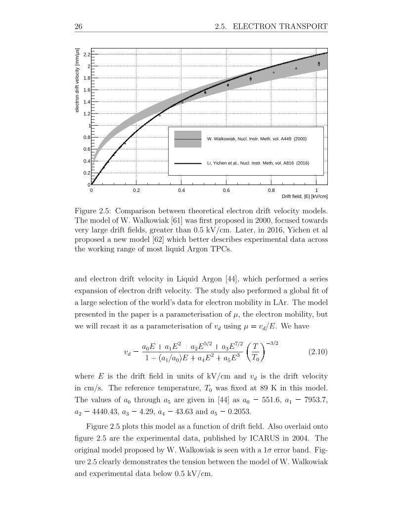
Figure 2.5: Comparison between theoretical electron drift velocity models.The model of W. Walkowiak [61] was first proposed in 2000, focused towardsvery large drift fields, greater than 0.5 kV/cm. Later, in 2016, Yichen et alproposed a new model [62] which better describes experimental data acrossthe working range of most liquid Argon TPCs.
and electron drift velocity in Liquid Argon [44], which performed a series
expansion of electron drift velocity. The study also performed a global fit of
a large selection of the world’s data for electron mobility in LAr. The model
presented in the paper is a parameterisation of µ, the electron mobility, but
we will recast it as a parameterisation of vd using µ vdE. We have
vd a0E a1E
2 a2E52 a3E
72
1 pa1a0qE a4E2 a5E
3
T
T0
32
(2.10)
where E is the drift field in units of kV/cm and vd is the drift velocity
in cm/s. The reference temperature, T0 was fixed at 89 K in this model.
The values of a0 through a5 are given in [44] as a0 551.6, a1 7953.7,
a2 4440.43, a3 4.29, a4 43.63 and a5 0.2053.
Figure 2.5 plots this model as a function of drift field. Also overlaid onto
figure 2.5 are the experimental data, published by ICARUS in 2004. The
original model proposed by W. Walkowiak is seen with a 1σ error band. Fig-
ure 2.5 clearly demonstrates the tension between the model of W. Walkowiak
and experimental data below 0.5 kV/cm.
2.5. ELECTRON TRANSPORT 27
2.5.2 Electron diffusion
Throughout the process of drifting, a charge cloud will diffuse in both longi-
tudinal and transverse planes. The parameter DL describes the diffusion in
the longitudinal plane, the drift direction, and the parameter DT describes
the diffusion in the transverse plane, perpendicular to the drift. Both trans-
verse and longitudinal diffusion is Gaussian in space, with standard devia-
tions given by
σT a
2DT t (2.11)
σL a
2DLt (2.12)
The most successful parameterisation of DT and DL is proposed in [44],
and can be written as
DL a0 a1E a2E
32 a3E52
1 pa1a0qE a4E2 a5E
3
b0 b1E b2E
2
1 pb1b0qE b3E2
T
T1
T
T0
32
(2.13)
where we have two reference temperatures, T0 and T1. This is an artifact
from the methodology used to produce this parameterisation. First, a global
fit was performed on electron mobility, µ. For this global fit, a reference
temperature of T0 89 K is used. Next, a secondary parameterisation was
developed for the effective longitudinal electron energy, εL. For this param-
eterisation, the more suitable reference temperature was T1 87 K. Thus,
when determining DL µεLe, two reference temperatures are introduced.
The parameterisation for DT is not given directly, but DL and DT are
related according to
DT DL
1 EµBµBE
(2.14)
The derivation ofDT , although relatively straightforward, is protracted. The
result can be found in Appendix A.
We can see from Equation 2.13 that both DL and DT are dependent
on both the temperature of the Liquid Argon and the applied drift field.
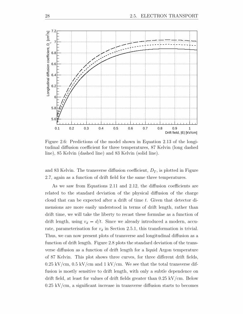
The Longitudinal diffusion coefficient, DL, is plotted in Figure 2.6 as a
function of drift field for three different temperatures, 87 Kelvin, 85 Kelvin
28 2.5. ELECTRON TRANSPORT
0.1 0.2 0.3 0.4 0.5 0.6 0.7 0.8 0.9 1Drift field, |E| [kV/cm]
5.6
5.8
6
6.2
6.4
6.6
6.8
7
7.2
/s]
2 [c
mL
Long
itudi
nal d
iffus
ion
coef
ficie
nt, D
Figure 2.6: Predictions of the model shown in Equation 2.13 of the longi-tudinal diffusion coefficient for three temperatures, 87 Kelvin (long dashedline), 85 Kelvin (dashed line) and 83 Kelvin (solid line).
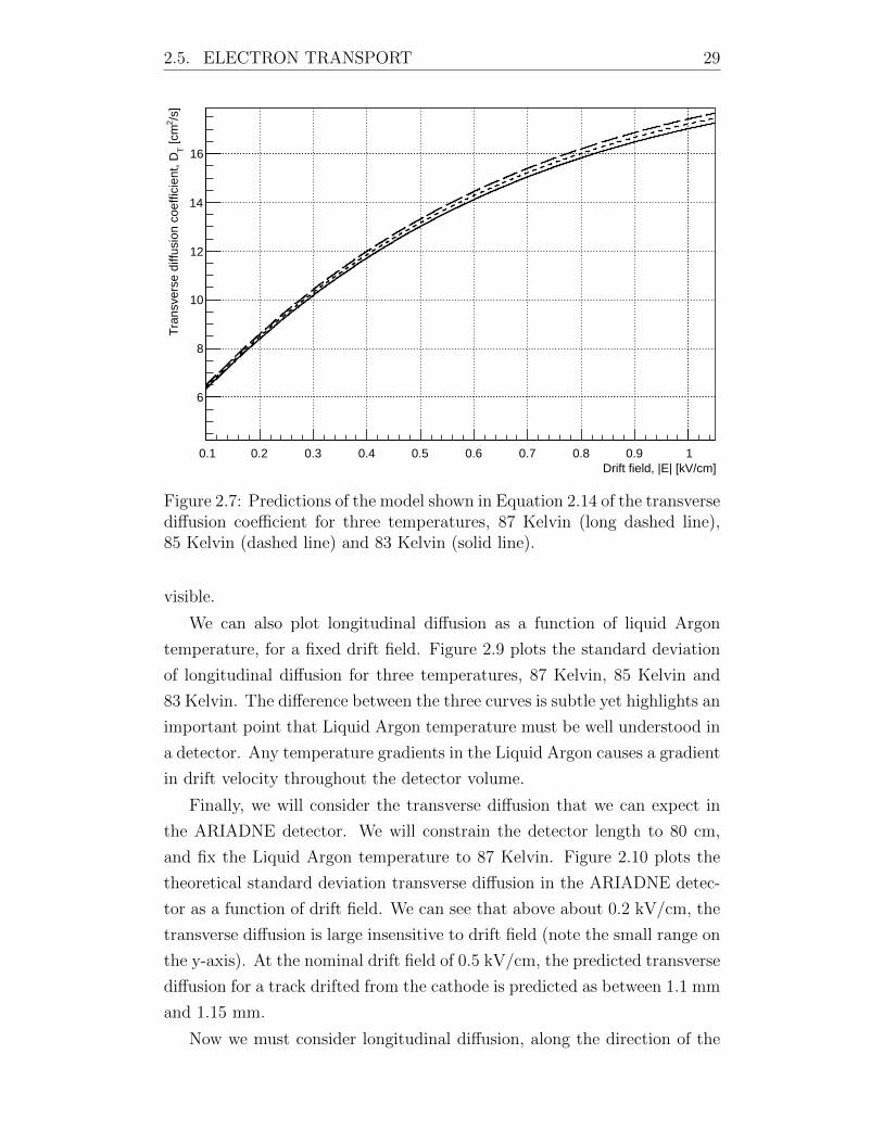
and 83 Kelvin. The transverse diffusion coefficient, DT , is plotted in Figure
2.7, again as a function of drift field for the same three temperatures.
As we saw from Equations 2.11 and 2.12, the diffusion coefficients are
related to the standard deviation of the physical diffusion of the charge
cloud that can be expected after a drift of time t. Given that detector di-
mensions are more easily understood in terms of drift length, rather than
drift time, we will take the liberty to recast these formulae as a function of
drift length, using vd dt. Since we already introduced a modern, accu-
rate, parameterisation for vd in Section 2.5.1, this transformation is trivial.
Thus, we can now present plots of transverse and longitudinal diffusion as a
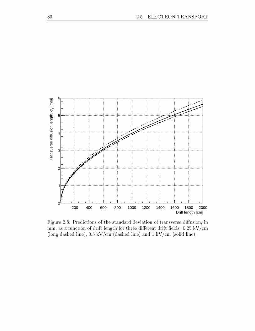
function of drift length. Figure 2.8 plots the standard deviation of the trans-
verse diffusion as a function of drift length for a liquid Argon temperature
of 87 Kelvin. This plot shows three curves, for three different drift fields,
0.25 kV/cm, 0.5 kV/cm and 1 kV/cm. We see that the total transverse dif-
fusion is mostly sensitive to drift length, with only a subtle dependence on
drift field, at least for values of drift fields greater than 0.25 kV/cm. Below
0.25 kV/cm, a significant increase in transverse diffusion starts to becomes
2.5. ELECTRON TRANSPORT 29
0.1 0.2 0.3 0.4 0.5 0.6 0.7 0.8 0.9 1Drift field, |E| [kV/cm]
6
8
10
12
14
16
/s]
2 [c
mT
Tra
nsve
rse
diffu
sion
coe
ffici
ent,
D
Figure 2.7: Predictions of the model shown in Equation 2.14 of the transversediffusion coefficient for three temperatures, 87 Kelvin (long dashed line),85 Kelvin (dashed line) and 83 Kelvin (solid line).
visible.
We can also plot longitudinal diffusion as a function of liquid Argon
temperature, for a fixed drift field. Figure 2.9 plots the standard deviation
of longitudinal diffusion for three temperatures, 87 Kelvin, 85 Kelvin and
83 Kelvin. The difference between the three curves is subtle yet highlights an
important point that Liquid Argon temperature must be well understood in
a detector. Any temperature gradients in the Liquid Argon causes a gradient
in drift velocity throughout the detector volume.
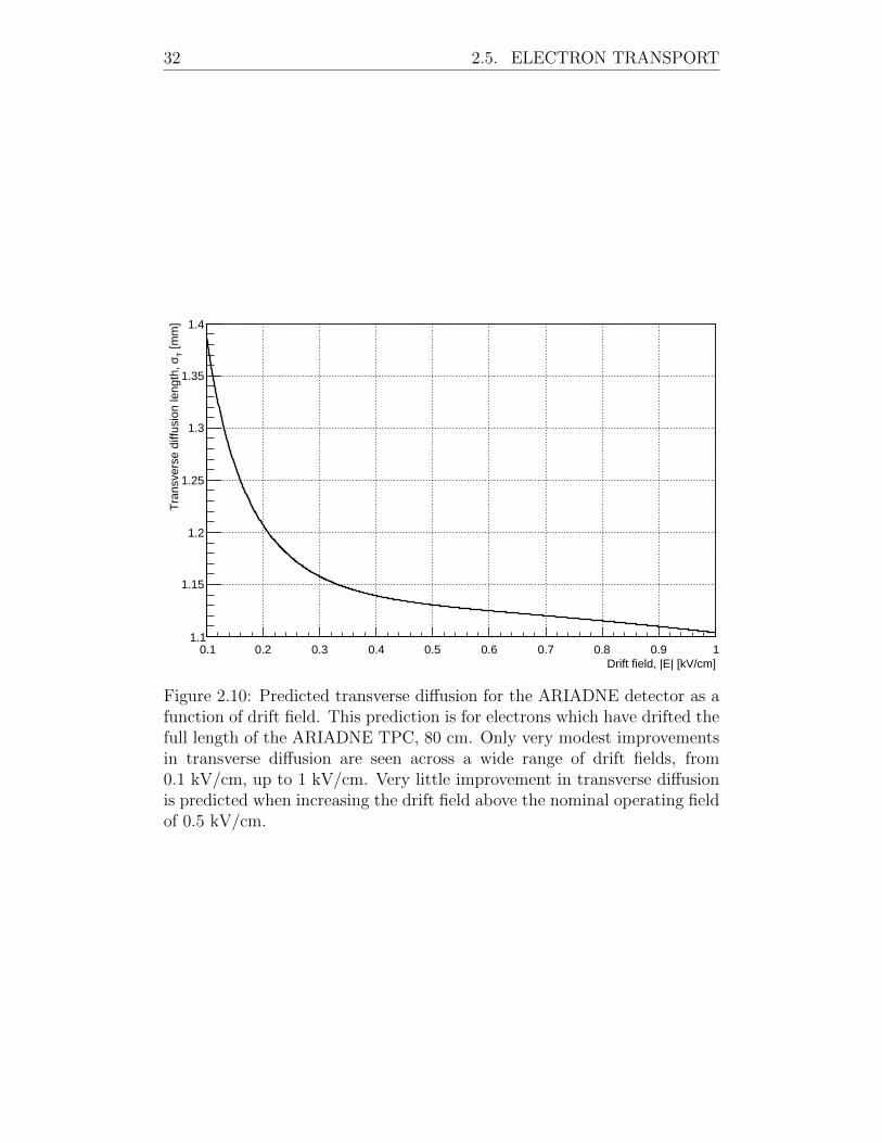
Finally, we will consider the transverse diffusion that we can expect in
the ARIADNE detector. We will constrain the detector length to 80 cm,
and fix the Liquid Argon temperature to 87 Kelvin. Figure 2.10 plots the
theoretical standard deviation transverse diffusion in the ARIADNE detec-
tor as a function of drift field. We can see that above about 0.2 kV/cm, the
transverse diffusion is large insensitive to drift field (note the small range on
the y-axis). At the nominal drift field of 0.5 kV/cm, the predicted transverse
diffusion for a track drifted from the cathode is predicted as between 1.1 mm
and 1.15 mm.
Now we must consider longitudinal diffusion, along the direction of the
30 2.5. ELECTRON TRANSPORT
200 400 600 800 1000 1200 1400 1600 1800 2000Drift length [cm]
0
1
2
3
4
5
6
[mm
]Tσ
Tra
nsve
rse
diffu
sion
leng
th,
Figure 2.8: Predictions of the standard deviation of transverse diffusion, inmm, as a function of drift length for three different drift fields: 0.25 kV/cm(long dashed line), 0.5 kV/cm (dashed line) and 1 kV/cm (solid line).

2.5. ELECTRON TRANSPORT 31
0 200 400 600 800 1000 1200 1400 1600 1800 2000Drift length [cm]
0
1
2
3
4
5
6
[mm
]Tσ
Tra
nsve
rse
diffu
sion
leng
th,
Figure 2.9: Predictions of the standard deviation of transverse diffusion, inmm, as a function of drift length for three different Liquid Argon tempera-tures: 87 Kelvin (dashed line), 85 Kelvin (long dashed line) and 83 Kelvin(solid line).
32 2.5. ELECTRON TRANSPORT
0.1 0.2 0.3 0.4 0.5 0.6 0.7 0.8 0.9 1Drift field, |E| [kV/cm]
1.1
1.15
1.2
1.25
1.3
1.35
1.4
[mm
]Tσ
Tra
nsve
rse
diffu
sion
leng
th,
Figure 2.10: Predicted transverse diffusion for the ARIADNE detector as afunction of drift field. This prediction is for electrons which have drifted thefull length of the ARIADNE TPC, 80 cm. Only very modest improvementsin transverse diffusion are seen across a wide range of drift fields, from0.1 kV/cm, up to 1 kV/cm. Very little improvement in transverse diffusionis predicted when increasing the drift field above the nominal operating fieldof 0.5 kV/cm.
2.5. ELECTRON TRANSPORT 33
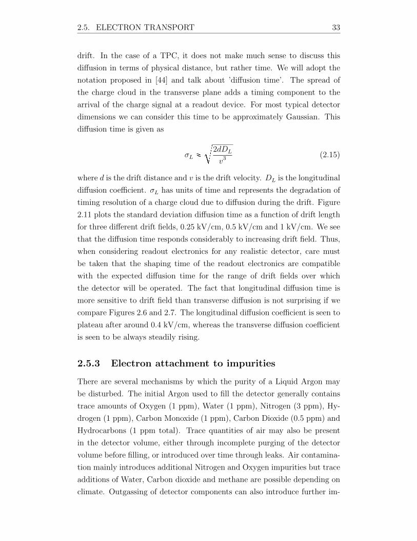
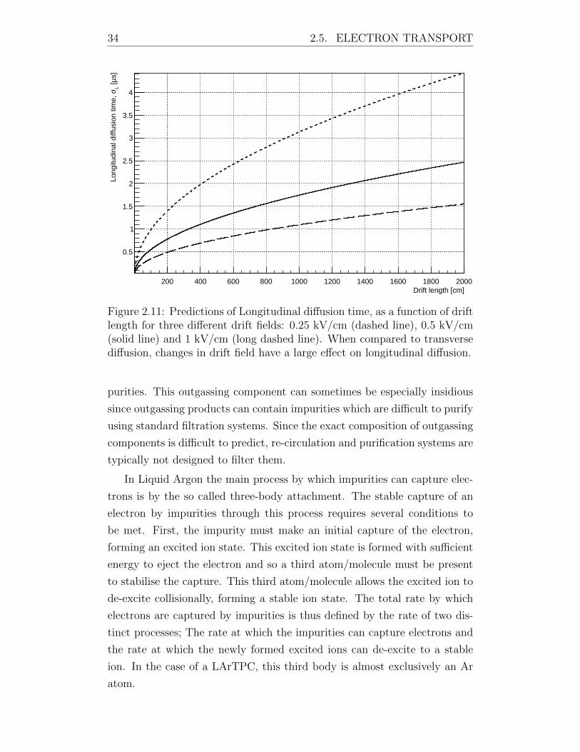
drift. In the case of a TPC, it does not make much sense to discuss this
diffusion in terms of physical distance, but rather time. We will adopt the
notation proposed in [44] and talk about ’diffusion time’. The spread of
the charge cloud in the transverse plane adds a timing component to the
arrival of the charge signal at a readout device. For most typical detector
dimensions we can consider this time to be approximately Gaussian. This
diffusion time is given as
σL c
2dDL
v3 (2.15)
where d is the drift distance and v is the drift velocity. DL is the longitudinal
diffusion coefficient. σL has units of time and represents the degradation of
timing resolution of a charge cloud due to diffusion during the drift. Figure
2.11 plots the standard deviation diffusion time as a function of drift length
for three different drift fields, 0.25 kV/cm, 0.5 kV/cm and 1 kV/cm. We see
that the diffusion time responds considerably to increasing drift field. Thus,
when considering readout electronics for any realistic detector, care must
be taken that the shaping time of the readout electronics are compatible
with the expected diffusion time for the range of drift fields over which
the detector will be operated. The fact that longitudinal diffusion time is
more sensitive to drift field than transverse diffusion is not surprising if we
compare Figures 2.6 and 2.7. The longitudinal diffusion coefficient is seen to
plateau after around 0.4 kV/cm, whereas the transverse diffusion coefficient
is seen to be always steadily rising.
2.5.3 Electron attachment to impurities
There are several mechanisms by which the purity of a Liquid Argon may
be disturbed. The initial Argon used to fill the detector generally contains
trace amounts of Oxygen (1 ppm), Water (1 ppm), Nitrogen (3 ppm), Hy-
drogen (1 ppm), Carbon Monoxide (1 ppm), Carbon Dioxide (0.5 ppm) and
Hydrocarbons (1 ppm total). Trace quantities of air may also be present
in the detector volume, either through incomplete purging of the detector
volume before filling, or introduced over time through leaks. Air contamina-
tion mainly introduces additional Nitrogen and Oxygen impurities but trace
additions of Water, Carbon dioxide and methane are possible depending on
climate. Outgassing of detector components can also introduce further im-
34 2.5. ELECTRON TRANSPORT
200 400 600 800 1000 1200 1400 1600 1800 2000Drift length [cm]
0.5
1
1.5
2
2.5
3
3.5
4
s]µ [ LσLo
ngitu
dina
l diff
usio
n tim
e,
Figure 2.11: Predictions of Longitudinal diffusion time, as a function of driftlength for three different drift fields: 0.25 kV/cm (dashed line), 0.5 kV/cm(solid line) and 1 kV/cm (long dashed line). When compared to transversediffusion, changes in drift field have a large effect on longitudinal diffusion.
purities. This outgassing component can sometimes be especially insidious
since outgassing products can contain impurities which are difficult to purify
using standard filtration systems. Since the exact composition of outgassing
components is difficult to predict, re-circulation and purification systems are
typically not designed to filter them.
In Liquid Argon the main process by which impurities can capture elec-
trons is by the so called three-body attachment. The stable capture of an
electron by impurities through this process requires several conditions to
be met. First, the impurity must make an initial capture of the electron,
forming an excited ion state. This excited ion state is formed with sufficient
energy to eject the electron and so a third atom/molecule must be present
to stabilise the capture. This third atom/molecule allows the excited ion to
de-excite collisionally, forming a stable ion state. The total rate by which
electrons are captured by impurities is thus defined by the rate of two dis-
tinct processes; The rate at which the impurities can capture electrons and
the rate at which the newly formed excited ions can de-excite to a stable
ion. In the case of a LArTPC, this third body is almost exclusively an Ar
atom.
2.5. ELECTRON TRANSPORT 35
The rate by which electronegative impurities capture electrons is defined
by a rate constant, k. Since the cross section of the electron capture process
is dependent on the kinetic energy of the drifting electron, k is a function of
the drift field. The rate of electron loss in the TPC is related to k according
the following differential equation
BNBt kN (2.16)
Although it would seem that a theoretical framework exists for predicting
k for various impurities in Liquid Argon [63], all of the currently available
information is the result of direct experimental measurements of k for various
impurities. As a result, k is only known for a certain subset of impurities.
Equation 2.16 has the solution
N N0ekt (2.17)
where, if we now define the electron lifetime as τ 1k, we have
N N0etτ (2.18)
Electron lifetime is the probably the most commonly used parameter to
quantify the effect of impurities in a LArTPC.
Summarising results from [64], at 0.5 kV/cm; The attachment rate of
Oxygen is almost an order of magnitude higher than Nitrous oxide. Again
at 0.5 kV/cm, the rate constant for carbon dioxide is more than an order of
magnitude lower than that of Oxygen [65]. The attachment rate of Sulfur
hexafluoride is very high, almost three orders of magnitude more than Oxy-
gen but this molecule is rare in commercial LAr, although may be present
in air at the ppt level [66]. Given that Oxygen makes up 20% of air, a
leak in a detector would cause more electrons to be lost by attachment to
Oxygen, even given the high attachment rate of Sulfur hexafluoride, due to
its exceptionally low trace presence in air. Nitrogen is assumed to not affect
drifting electrons, probably due to having no electronegativity [67]. Water
is known to attach to drifting electrons, [68] at a rate comparable to oxygen.
It has been suggested that water is the only significant contaminant that
is introduced by outgassing of materials [69]. It does not appear that the
attachment rate is known for any of Hydrogen, Carbon Monoxide or other
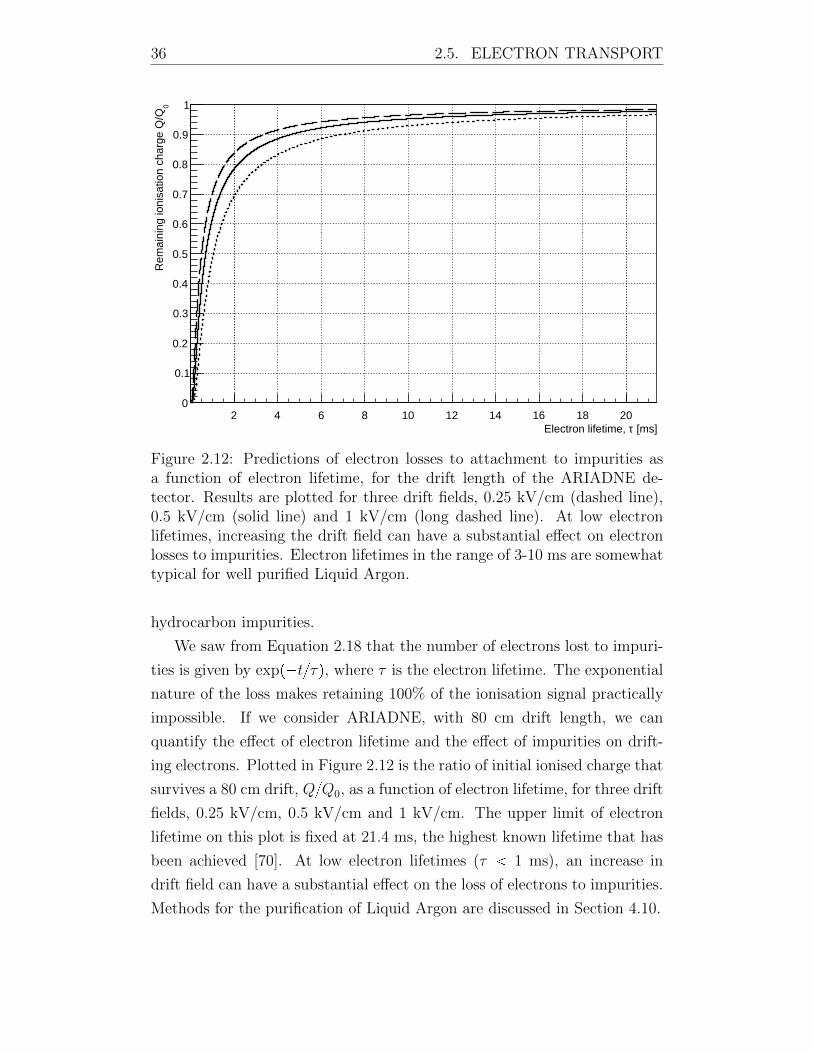
36 2.5. ELECTRON TRANSPORT
2 4 6 8 10 12 14 16 18 20 [ms]τElectron lifetime,
0
0.1
0.2
0.3
0.4
0.5
0.6
0.7
0.8
0.9
10R
emai
ning
ioni
satio
n ch
arge
Q/Q
Figure 2.12: Predictions of electron losses to attachment to impurities asa function of electron lifetime, for the drift length of the ARIADNE de-tector. Results are plotted for three drift fields, 0.25 kV/cm (dashed line),0.5 kV/cm (solid line) and 1 kV/cm (long dashed line). At low electronlifetimes, increasing the drift field can have a substantial effect on electronlosses to impurities. Electron lifetimes in the range of 3-10 ms are somewhattypical for well purified Liquid Argon.
hydrocarbon impurities.
We saw from Equation 2.18 that the number of electrons lost to impuri-
ties is given by expptτq, where τ is the electron lifetime. The exponential
nature of the loss makes retaining 100% of the ionisation signal practically
impossible. If we consider ARIADNE, with 80 cm drift length, we can
quantify the effect of electron lifetime and the effect of impurities on drift-
ing electrons. Plotted in Figure 2.12 is the ratio of initial ionised charge that
survives a 80 cm drift, QQ0, as a function of electron lifetime, for three drift
fields, 0.25 kV/cm, 0.5 kV/cm and 1 kV/cm. The upper limit of electron
lifetime on this plot is fixed at 21.4 ms, the highest known lifetime that has
been achieved [70]. At low electron lifetimes (τ 1 ms), an increase in
drift field can have a substantial effect on the loss of electrons to impurities.
Methods for the purification of Liquid Argon are discussed in Section 4.10.
2.6. SINGLE PHASE READOUT 37
2.6 Single phase readout
Given the nature of this Thesis, single phase readout will be discussed only
in passing to provide a more complete context of Liquid Argon detector
technologies. Single phase detectors rely on placing charge readout devices in
the Liquid Argon phase. Thus, the signal that is created in the liquid phase
is readout in the Liquid phase. There is some freedom in which approach
is used to readout the charge signal, for example pixel based or strip (wire)
based readout. By far the most common approach has been strip (wire)
based, although pixel based readout has been explored recently [71]. We
will focus here on strip (wire) based readout.
In order to reconstruct an event in a LArTPC with a strip based readout
approach, two (or more) readout planes are required. With a single wire,
there is ambiguity about where along the wire the signal was received from.
To combat this ambiguity, another plane of wires, rotated at an angle relative
to the first, can be used to constrain the position on the wire where the signal
originates from. Several parameters are tunable when designing such a wire
based readout approach including the spacing between wires and the relative
angle between both wires planes. A popular approach is to use three wires
planes, arranged roughly 30-40 degrees relative to one another. The use of
three wire planes over two provides improved reconstruction capability and
reduced possibility of ambiguities.
In order to maximise signal collection efficiency, two wire planes can be
biased to a positive voltage. When an electron cloud passes by these wires,
it is deflected around them. The signal on this wire is caused by induction,
rather than collection. The final plane of wires performs charge collection.
Thus, there are two induction planes and one collection plane.
Single phase readout has a very successful history, with almost all of
the historically famous detectors being readout in this way. Well known
examples include ICARUS [72], MicroBooNE [73], SBND [74] and Single-
Phase ProtoDUNE [75].
38 2.7. DUAL-PHASE READOUT
2.7 Dual-phase readout
Dual-phase TPCs were proposed as a way to exploit developments in mi-
cropattern gas detectors (MPGDs). As their name would suggest, MPGDs
generally perform best in a gas phase. Severely reduced performance is how-
ever still possible in the liquid phase. To take full advantage of a MPGD,
the electron signal in the Liquid argon must be transferred from the liquid
phase to the gas phase, by a process known as electron extraction.
2.7.1 Extraction of electrons from liquid to gas
The emission of electrons from the liquid to gas phase has been well stud-
ied [76]. The process is known to have two components in time. The first
emission component, which is very fast, Opnsq, is the combination of several
processes, all of which happen on a fast timescale. In order for an elec-
tron to cross the Liquid/gas interface it must have sufficient kinetic energy,
perpendicular to the interface. This condition gives rise to an electric field
dependence of the electron extraction efficiency. At higher electric fields,
the electrons are more energetic and are therefore more likely to meet the
emission condition. The extraction of electrons which meet the emission
condition is very fast, Opnsq. It is possible that, on the first attempt, the
electrons do not meet the emission condition, perhaps due to a collision with
an Argon atom very close to the interface, resulting in the electron having
insufficient kinetic energy perpendicular to the interface to be extracted. In
case the electrons do not meet the emission condition, they will be reflected
off the interface. Following this reflection, the electrons are again acceler-
ated towards the boundary by the electric field. Depending on the collisions
experienced between the electrons and the Argon atoms near the interface,
it may take several repeated attempts before the electrons meet the emission
condition and are extracted. These repeated reflections occur very quickly,
Opnsq. The fast component of electron emission is the sum of those electrons
which are directly emitted over the potential barrier on the first attempt, as
well as those electrons which reflect off the potential barrier but eventually,
after one or several reflections, meet the emission criteria and are extracted
into the gas phase.
Each reflection at the boundary causes the electrons to lose a small frac-
tion of their kinetic energy. If, after many collisions, the electrons still
2.7. DUAL-PHASE READOUT 39
never meet the emission criteria, they may lose enough energy as to be-
come trapped at the boundary. The electrons will continue to reflect off
the boundary, with energy provided by the electric field. The slow compo-
nent of electron emission results from these electrons which fail to cross the
potential barrier, even after repeated attempts. These ’cold’ electrons are
eventually emitted by thermionic emission. The electrons are ’heated’ by
the applied electric field across the boundary. The probability, and thus the
rate, of electron emission across the boundary depends on the magnitude of
the applied electric field.
Experimental data for the emission time constant for electrons as a func-
tion of electric field in Liquid Argon is quite limited. [77] presents the most
comprehensive dataset in the range 0.1 - 0.5 kV/cm. Extension of measure-
ments beyond this range were more recently performed [76], extending the
measured range up to 1.71 kV/cm. Although some measurements appear
to extend the tested range up to 4 kV/cm [78], the test procedure was not
sensitive to the emission time constant. Several models have been proposed
to describe the emission time as a function of electric field. The first, and
most simple model, predicts that
τ λ1
µEexp
V0
kBT
(2.19)
where λ1 is the electron mean free path in the Liquid, µ is the electron
mobility, E is the electric field in the extraction region, V0 is the potential
barrier at the liquid/gas interface, kB is Boltzmann’s constant and T is the
liquid Argon temperature. When attempting to fit this model to experimen-
tal data, µ is often treated as a constant as a function of E. Although we
now know this to not be true, this assumption was typical at the time when
this model was proposed [76] and [77]. This assumption allows us describe
the model in terms of a single free parameter, A, as
τ A
E(2.20)
The result of such a fit to experimental data can be seen in Figure 2.13.
Although perhaps reasonable at higher fields, the tension is clear. Thus, we
can probably conclude that either that the model is not appropriate or that
the assumption that µ is a constant is invalid. Given that, in Section 2.5.1,
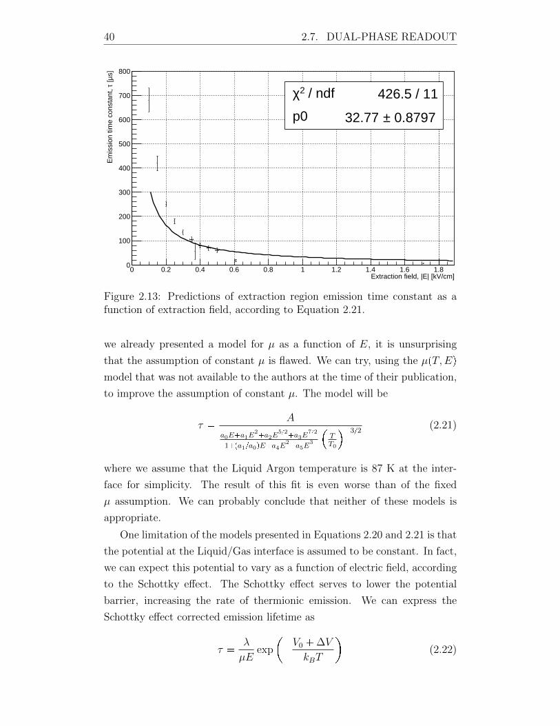
40 2.7. DUAL-PHASE READOUT
0 0.2 0.4 0.6 0.8 1 1.2 1.4 1.6 1.8Extraction field, |E| [kV/cm]
0
100
200
300
400
500
600
700
800s]µ [τE
mis
sion
tim
e co
nsta
nt, / ndf 2χ 426.5 / 11
p0 0.8797± 32.77
/ ndf 2χ 426.5 / 11
p0 0.8797± 32.77
Figure 2.13: Predictions of extraction region emission time constant as afunction of extraction field, according to Equation 2.21.
we already presented a model for µ as a function of E, it is unsurprising
that the assumption of constant µ is flawed. We can try, using the µpT,Eqmodel that was not available to the authors at the time of their publication,
to improve the assumption of constant µ. The model will be
τ A
a0Ea1E2a2E
52a3E
72
1pa1a0qEa4E2a5E
3
TT0
32(2.21)
where we assume that the Liquid Argon temperature is 87 K at the inter-
face for simplicity. The result of this fit is even worse than of the fixed
µ assumption. We can probably conclude that neither of these models is
appropriate.
One limitation of the models presented in Equations 2.20 and 2.21 is that
the potential at the Liquid/Gas interface is assumed to be constant. In fact,
we can expect this potential to vary as a function of electric field, according
to the Schottky effect. The Schottky effect serves to lower the potential
barrier, increasing the rate of thermionic emission. We can express the
Schottky effect corrected emission lifetime as
τ λ
µEexp
V0 ∆V
kBT
(2.22)
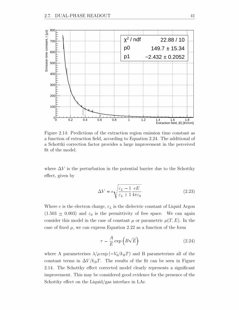
2.7. DUAL-PHASE READOUT 41
0 0.2 0.4 0.6 0.8 1 1.2 1.4 1.6 1.8Extraction field, |E| [kV/cm]
0
100
200
300
400
500
600
700
800s]µ [τE
mis
sion
tim
e co
nsta
nt, / ndf 2χ 22.88 / 10
p0 15.34± 149.7
p1 0.2052±2.432 −
/ ndf 2χ 22.88 / 10
p0 15.34± 149.7
p1 0.2052±2.432 −
Figure 2.14: Predictions of the extraction region emission time constant asa function of extraction field, according to Equation 2.24. The additional ofa Schottki correction factor provides a large improvement in the perceivedfit of the model.
where ∆V is the perturbation in the potential barrier due to the Schottky
effect, given by
∆V e
dεL 1
εL 1
eE
4πε0
(2.23)
Where e is the electron charge, εL is the dielectric constant of Liquid Argon
(1.503 0.003) and ε0 is the permittivity of free space. We can again
consider this model in the case of constant µ or parametric µpT,Eq. In the
case of fixed µ, we can express Equation 2.22 as a function of the form
τ A
Eexp
B?E
(2.24)
where A parameterises λµ exp pV0kBT q and B parameterises all of the
constant terms in ∆V kBT . The results of the fit can be seen in Figure
2.14. The Schottky effect corrected model clearly represents a significant
improvement. This may be considered good evidence for the presence of the
Schottky effect on the Liquid/gas interface in LAr.
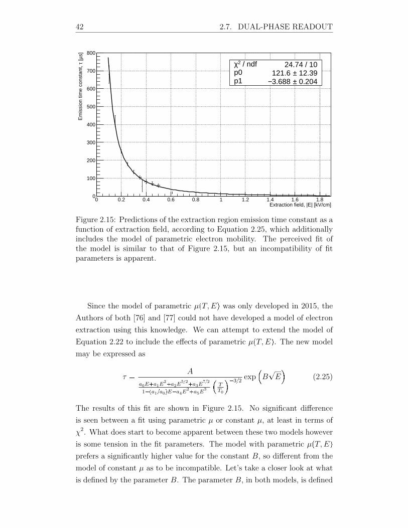
42 2.7. DUAL-PHASE READOUT
0 0.2 0.4 0.6 0.8 1 1.2 1.4 1.6 1.8Extraction field, |E| [kV/cm]
0
100
200
300
400
500
600
700
800s]µ [τE
mis
sion
tim
e co
nsta
nt, / ndf 2χ 24.74 / 10
p0 12.39± 121.6 p1 0.204±3.688 −
/ ndf 2χ 24.74 / 10p0 12.39± 121.6 p1 0.204±3.688 −
Figure 2.15: Predictions of the extraction region emission time constant as afunction of extraction field, according to Equation 2.25, which additionallyincludes the model of parametric electron mobility. The perceived fit ofthe model is similar to that of Figure 2.15, but an incompatibility of fitparameters is apparent.
Since the model of parametric µpT,Eq was only developed in 2015, the
Authors of both [76] and [77] could not have developed a model of electron
extraction using this knowledge. We can attempt to extend the model of
Equation 2.22 to include the effects of parametric µpT,Eq. The new model
may be expressed as
τ A
a0Ea1E2a2E
52a3E
72
1pa1a0qEa4E2a5E
3
TT0
32exp
B?E
(2.25)
The results of this fit are shown in Figure 2.15. No significant difference
is seen between a fit using parametric µ or constant µ, at least in terms of
χ2. What does start to become apparent between these two models however
is some tension in the fit parameters. The model with parametric µpT,Eqprefers a significantly higher value for the constant B, so different from the
model of constant µ as to be incompatible. Let’s take a closer look at what
is defined by the parameter B. The parameter B, in both models, is defined
2.7. DUAL-PHASE READOUT 43
as
B eb
εL1εL1
e4πε0
kBT(2.26)
Given that every term in this expression is known, we can compare the
prediction of this value from the fit to what is expected based on known
values of the constants. We can calculate the parameter B, in Liquid Argon,
should be given as
B eb
1.50511.5051
e4πε0
kBT 0.717
acm/kV (2.27)
Neither model does a good job at describing this constant. We can again
most likely conclude that these models are nonphysical, even if they quali-
tatively do a good job of describing the shape of the data.
An extension to the extraction model, proposed in [76], is that an addi-
tional term must be included to factor in electrons which, once extracted,
collide with a gas Argon atom and rebound back into the liquid phase,
becoming trapped once again. This additional term serves to extend the
emission lifetime. This term is introduced through an additional factor of
Cx, giving the new model a Ax2 exppB?Eq dependence. The result of
fitting this function to the data, again with a constant µ approximation,
is shown in Figure 2.16. This new model is makes a much more physical
prediction of the parameter B, which is now compatible with the expected
value. In fact, we can argue that the parameter B should not even be a
parameter at all. If we fix B to 0.717a
cm/kV, the model still does an
acceptable job of describing the experimental data.
Of course, we must now interpret this discussion in view of the operation
of a LArTPC. Results from [78] are often quoted, potentially inaccurately,
that an extraction field of 3 - 4 kV/cm provides 100 % extraction efficiency.
Whilst this may have been true for the experimental setup of [78], caution
must be used when extrapolating this value to other detectors. We have
already seen in this section that electron emission in the extraction region
occurs over a characteristic timescale. The collection efficiency should more
realistically described as the fraction of electrons which have been emitted
within the integration time of the detector readout device. Integrating for
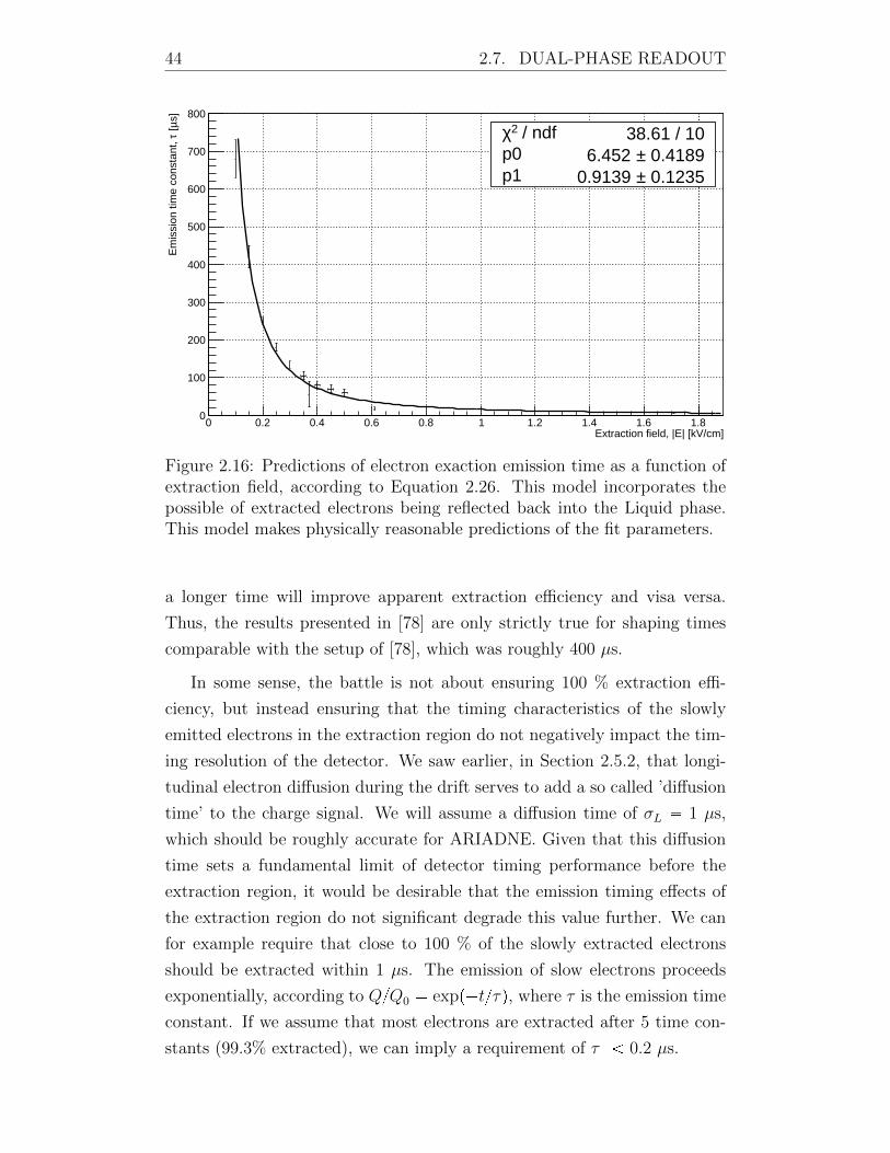
44 2.7. DUAL-PHASE READOUT
0 0.2 0.4 0.6 0.8 1 1.2 1.4 1.6 1.8Extraction field, |E| [kV/cm]
0
100
200
300
400
500
600
700
800s]µ [τE
mis
sion
tim
e co
nsta
nt, / ndf 2χ 38.61 / 10
p0 0.4189± 6.452 p1 0.1235± 0.9139
/ ndf 2χ 38.61 / 10p0 0.4189± 6.452 p1 0.1235± 0.9139
Figure 2.16: Predictions of electron exaction emission time as a function ofextraction field, according to Equation 2.26. This model incorporates thepossible of extracted electrons being reflected back into the Liquid phase.This model makes physically reasonable predictions of the fit parameters.
a longer time will improve apparent extraction efficiency and visa versa.
Thus, the results presented in [78] are only strictly true for shaping times
comparable with the setup of [78], which was roughly 400 µs.
In some sense, the battle is not about ensuring 100 % extraction effi-
ciency, but instead ensuring that the timing characteristics of the slowly
emitted electrons in the extraction region do not negatively impact the tim-
ing resolution of the detector. We saw earlier, in Section 2.5.2, that longi-
tudinal electron diffusion during the drift serves to add a so called ’diffusion
time’ to the charge signal. We will assume a diffusion time of σL 1 µs,
which should be roughly accurate for ARIADNE. Given that this diffusion
time sets a fundamental limit of detector timing performance before the
extraction region, it would be desirable that the emission timing effects of
the extraction region do not significant degrade this value further. We can
for example require that close to 100 % of the slowly extracted electrons
should be extracted within 1 µs. The emission of slow electrons proceeds
exponentially, according to QQ0 expptτq, where τ is the emission time
constant. If we assume that most electrons are extracted after 5 time con-
stants (99.3% extracted), we can imply a requirement of τ 0.2 µs.
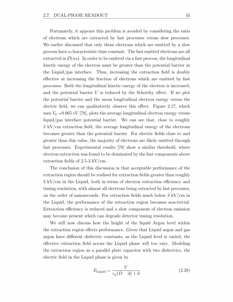
2.7. DUAL-PHASE READOUT 45
Fortunately, it appears this problem is avoided by considering the ratio
of electrons which are extracted by fast processes versus slow processes.
We earlier discussed that only those electrons which are emitted by a slow
process have a characteristic time constant. The fast emitted electrons are all
extracted inOpnsq. In order to be emitted via a fast process, the longitudinal
kinetic energy of the electron must be greater than the potential barrier at
the Liquid/gas interface. Thus, increasing the extraction field is doubly
effective at increasing the fraction of electrons which are emitted by fast
processes. Both the longitudinal kinetic energy of the electron is increased,
and the potential barrier V is reduced by the Schottky effect. If we plot
the potential barrier and the mean longitudinal electron energy versus the
electric field, we can qualitatively observe this effect. Figure 2.17, which
uses V0 0.065 eV [78], plots the average longitudinal electron energy versus
liquid/gas interface potential barrier. We can see that, close to roughly
3 kV/cm extraction field, the average longitudinal energy of the electrons
becomes greater than the potential barrier. For electric fields close to and
greater than this value, the majority of electrons are likely emitted through
fast processes. Experimental results [78] show a similar threshold, where
electron extraction was found to be dominated by the fast components above
extraction fields of 2.5-3 kV/cm.
The conclusion of this discussion is that acceptable performance of the
extraction region should be realised for extraction fields greater than roughly
3 kV/cm in the Liquid, both in terms of electron extraction efficiency and
timing resolution, with almost all electrons being extracted by fast processes,
on the order of nanoseconds. For extraction fields much below 3 kV/cm in
the Liquid, the performance of the extraction region becomes non-trivial.
Extraction efficiency is reduced and a slow component of electron emission
may become present which can degrade detector timing resolution.
We will now discuss how the height of the liquid Argon level within
the extraction region effects performance. Given that Liquid argon and gas
argon have different dielectric constants, as the Liquid level is varied, the
effective extraction field across the Liquid phase will too vary. Modeling
the extraction region as a parallel plate capacitor with two dielectrics, the
electric field in the Liquid phase is given by
ELiquid V
εLpD dq d(2.28)
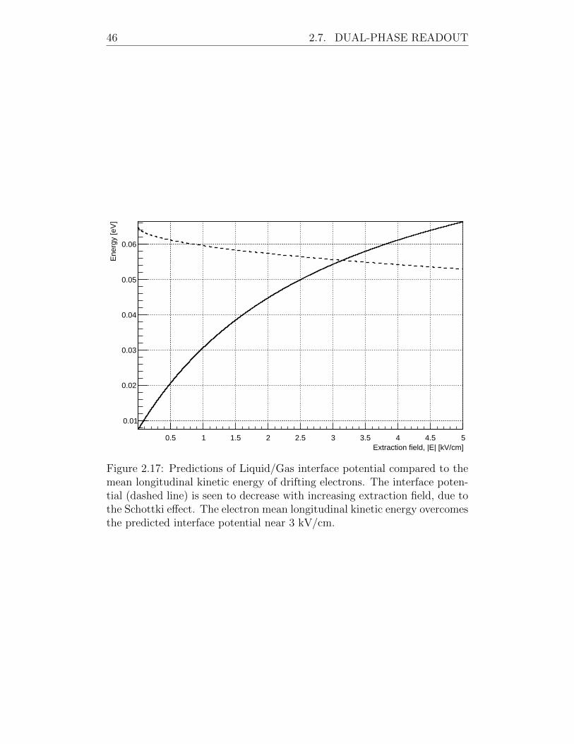
46 2.7. DUAL-PHASE READOUT
0.5 1 1.5 2 2.5 3 3.5 4 4.5 5Extraction field, |E| [kV/cm]
0.01
0.02
0.03
0.04
0.05
0.06
Ene
rgy
[eV
]
Figure 2.17: Predictions of Liquid/Gas interface potential compared to themean longitudinal kinetic energy of drifting electrons. The interface poten-tial (dashed line) is seen to decrease with increasing extraction field, due tothe Schottki effect. The electron mean longitudinal kinetic energy overcomesthe predicted interface potential near 3 kV/cm.
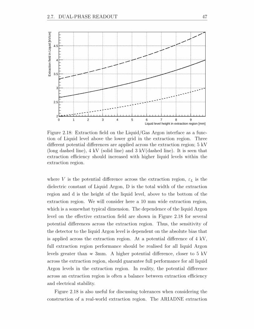
2.7. DUAL-PHASE READOUT 47
0 1 2 3 4 5 6 7 8 9Liquid level height in extraction region [mm]
2
2.5
3
3.5
4
4.5E
xtra
ctio
n fie
ld in
Liq
uid
[kV
/cm
]
Figure 2.18: Extraction field on the Liquid/Gas Argon interface as a func-tion of Liquid level above the lower grid in the extraction region. Threedifferent potential differences are applied across the extraction region; 5 kV(long dashed line), 4 kV (solid line) and 3 kV(dashed line). It is seen thatextraction efficiency should increased with higher liquid levels within theextraction region.
where V is the potential difference across the extraction region, εL is the
dielectric constant of Liquid Argon, D is the total width of the extraction
region and d is the height of the liquid level, above to the bottom of the
extraction region. We will consider here a 10 mm wide extraction region,
which is a somewhat typical dimension. The dependence of the liquid Argon
level on the effective extraction field are shown in Figure 2.18 for several
potential differences across the extraction region. Thus, the sensitivity of
the detector to the liquid Argon level is dependent on the absolute bias that
is applied across the extraction region. At a potential difference of 4 kV,
full extraction region performance should be realised for all liquid Argon
levels greater than 3mm. A higher potential difference, closer to 5 kV
across the extraction region, should guarantee full performance for all liquid
Argon levels in the extraction region. In reality, the potential difference
across an extraction region is often a balance between extraction efficiency
and electrical stability.
Figure 2.18 is also useful for discussing tolerances when considering the
construction of a real-world extraction region. The ARIADNE extraction
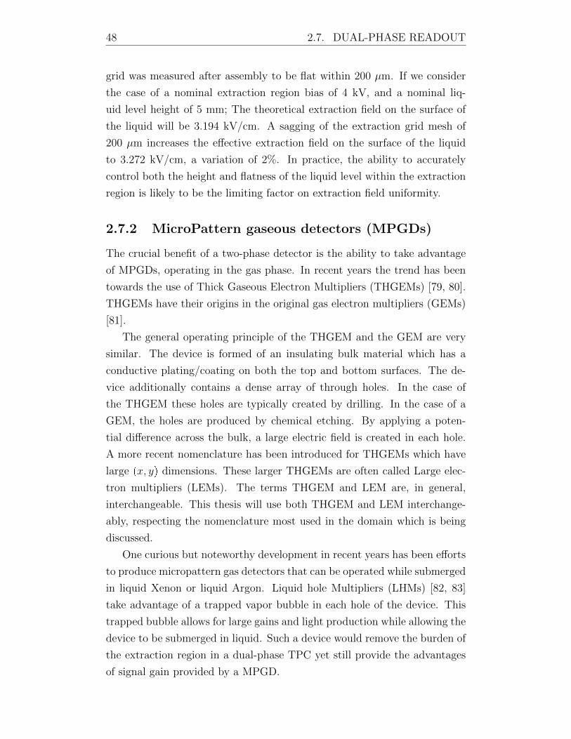
48 2.7. DUAL-PHASE READOUT
grid was measured after assembly to be flat within 200 µm. If we consider
the case of a nominal extraction region bias of 4 kV, and a nominal liq-
uid level height of 5 mm; The theoretical extraction field on the surface of
the liquid will be 3.194 kV/cm. A sagging of the extraction grid mesh of
200 µm increases the effective extraction field on the surface of the liquid
to 3.272 kV/cm, a variation of 2%. In practice, the ability to accurately
control both the height and flatness of the liquid level within the extraction
region is likely to be the limiting factor on extraction field uniformity.
2.7.2 MicroPattern gaseous detectors (MPGDs)
The crucial benefit of a two-phase detector is the ability to take advantage
of MPGDs, operating in the gas phase. In recent years the trend has been
towards the use of Thick Gaseous Electron Multipliers (THGEMs) [79, 80].
THGEMs have their origins in the original gas electron multipliers (GEMs)
[81].
The general operating principle of the THGEM and the GEM are very
similar. The device is formed of an insulating bulk material which has a
conductive plating/coating on both the top and bottom surfaces. The de-
vice additionally contains a dense array of through holes. In the case of
the THGEM these holes are typically created by drilling. In the case of a
GEM, the holes are produced by chemical etching. By applying a poten-
tial difference across the bulk, a large electric field is created in each hole.
A more recent nomenclature has been introduced for THGEMs which have
large px, yq dimensions. These larger THGEMs are often called Large elec-
tron multipliers (LEMs). The terms THGEM and LEM are, in general,
interchangeable. This thesis will use both THGEM and LEM interchange-
ably, respecting the nomenclature most used in the domain which is being
discussed.
One curious but noteworthy development in recent years has been efforts
to produce micropattern gas detectors that can be operated while submerged
in liquid Xenon or liquid Argon. Liquid hole Multipliers (LHMs) [82, 83]
take advantage of a trapped vapor bubble in each hole of the device. This
trapped bubble allows for large gains and light production while allowing the
device to be submerged in liquid. Such a device would remove the burden of
the extraction region in a dual-phase TPC yet still provide the advantages
of signal gain provided by a MPGD.
2.7. DUAL-PHASE READOUT 49
Charge readout of a two-phase TPC is generally performed using a seg-
mented anode. This segmented anode is placed a couple of millimeters above
the LEM. The separation between the LEM and the anode must be held with
a modest tolerance ( 5 %) to ensure a uniform electric field between the
LEM and the readout anode. Any deviations in this transfer field could
lead to deviations of the electron trajectory during transfer and introduce
uncertainties into event reconstruction. The anode currently proposed for
readout of a two-phase DUNE module is formed of many orthogonal strips,
with a strip to strip pitch of 3.125 mm [84]. These strips provide two distinct
views of the collected charge signal, and thus the event in the detector. The
strip geometry is constructed in such a way as to ensure that the collected
charge is shared evenly between both views. An intricate and elegant strip
geometry is used to minimise the strip length, and hence the strip capaci-
tance. Since strip capacitance is eventually related to the electronic noise
that can be expected, lowest possible strip capacitance is preferred. The cur-
rently proposed anode design has an estimated electronic noise of roughly
1000 electrons for the 2-m strip length.
Chapter 3
Optical readout
The most noteworthy aspect of the ARIADNE detector is the readout ap-
proach. As discussed earlier, typically, dual-phase TPCs are readout by
collecting charge on a segmented anode above the THGEM/LEM. The ARI-
ADNE detector instead exploits light that is produced during the electron
transfer process in the THGEM. The optical readout principle is shown in
Figure 3.1 in the simplest form. In general, a camera, placed at a mod-
est distance from the THGEM, collects the photons which are produced in
the THGEM holes. The distance between the camera and the THGEM is
constrained by the field of view of the imaging lens, the sensor size of the
camera and the desired px, yq detector area to be covered by a single camera.
A wider field of view allows more detector area to be covered, at the cost
of px, yq resolution. Multiple cameras may be tiled together to cover almost
arbitrarily large detector areas.
Optical TPCs are not a new concept. Many direct dark matter detec-
tion experiments already work using the optical readout principle. Recent
examples include LZ [23] and DarkSide [16]. The reason that this readout
principle has not seen more widespread use for the larger LArTPCs of neu-
trino oscillation physics is perhaps related to cost of scaling the approach
used by many dark matter experiments. These experiments, to achieve best
possible detection thresholds, generally use densely packed arrays of pho-
todetectors, very close to the location of light production. Scaling such a
geometry to a large, several meters by several meters detector, can become
prohibitively expensive. ARIADNE has been developing new methods and
technologies which allow for a single photodetector to cover a larger detec-
tor area. Thus, the cost of optical readout can be greatly reduced and the
50
51
readout approach becomes highly scalable. Additionally, the high resolution
of commercially available photodetectors, such as EMCCD and CCD cam-
eras, enables excellent x, y resolution. ARIADNE has found that the optical
readout devices can be placed far (¡1 m) from the point of light production,
while still retaining good detection thresholds. This allows the optical read-
out device to even be installed outside of the detector cryostat. This has
significant benefits in terms of maintenance, calibration and future upgrad-
ability of an experiment. No longer does the sensitive cryogenic volume of
the detector need to be disturbed for access to the readout device.
3.0.1 THGEM Light production
In low electric fields, electrons do not gain sufficient kinetic energy to ionise
Argon atoms. Instead, electron collisions with gas Argon atoms can only
cause excitation. Scintillation light is produced as the excited Argon atoms
de-excite, as earlier described in Section 2.4. As the electric field increases,
the electrons may gain enough kinetic energy to ionise Argon atoms, thus
releasing more electrons. These newly liberated electrons can, in turn, go
on to produce more ionisation. The resulting electron avalanche is known
as a Townsend discharge.
These two processes combine to give the THGEM a light output that is
linear, or proportional, at lower electric fields. Once in the Townsend regime,
exponential increasing light production occurs with increasing THGEM bias.
Although operation in the Townsend regime produces a large light signal,
there are some downsides. An unavoidable consequence of the production
of electrons by ionisation, is the production of ions. In Liquid Argon, the
mobility of ions is much much less than that of electrons [85], with drift
velocities as low as 1 cm/s in a typical 0.5 kV/cm drift field. Given this ex-
tremely slow drift velocity. Thus, these ions slowly drift backwards through
the TPC volume, remaining in the detector volume for extremely long pe-
riods of time. These ions may even accumulate to levels which can cause
issues with detector performance. If enough ions accumulate in the TPC vol-
ume, their presence can distort the drift field and alter the path of drifting
electrons. This effect is known as space charge.
Figure 3.2 shows the cross sections for excitation, ionisation and elastic
scattering of electrons on Argon atoms as a function of electron energy. At
very low energies, the dominant process is elastic scattering. This process
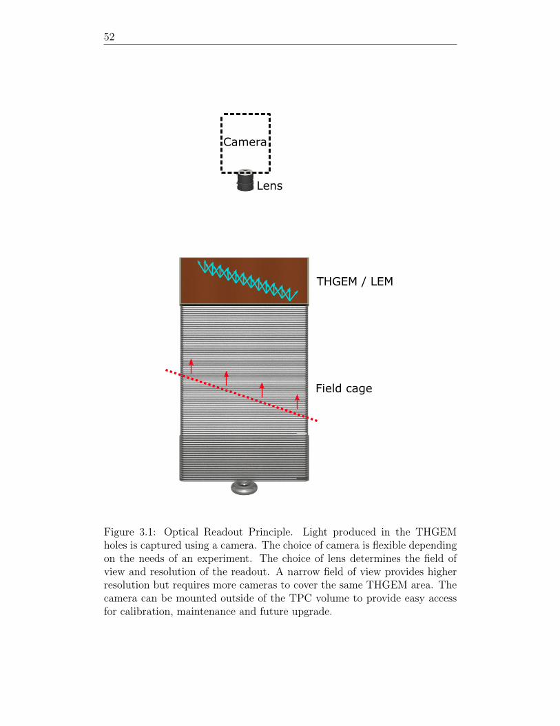
52
Camera
Lens
THGEM / LEM
Field cage
Figure 3.1: Optical Readout Principle. Light produced in the THGEMholes is captured using a camera. The choice of camera is flexible dependingon the needs of an experiment. The choice of lens determines the field ofview and resolution of the readout. A narrow field of view provides higherresolution but requires more cameras to cover the same THGEM area. Thecamera can be mounted outside of the TPC volume to provide easy accessfor calibration, maintenance and future upgrade.
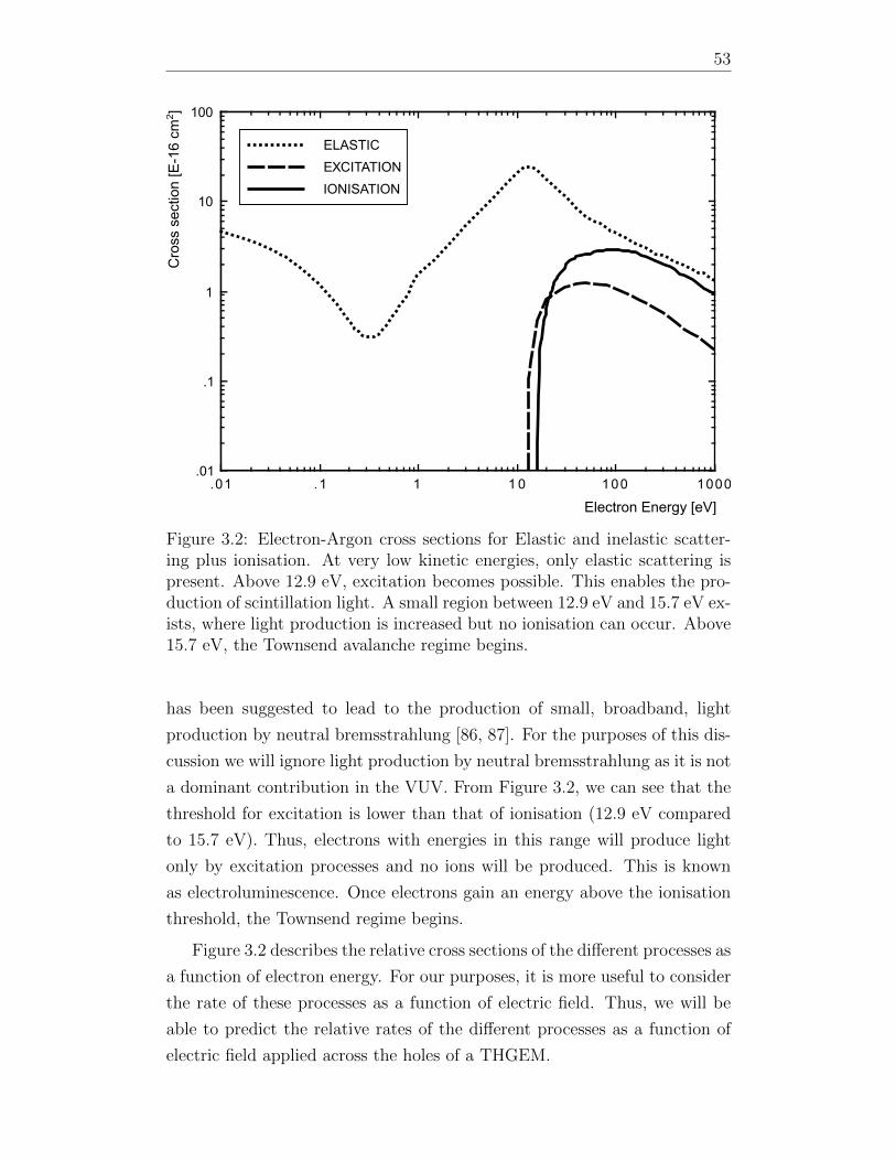
53
10001001 01.1.01.01
.1
1
10
100
IONISATION
EXCITATION
ELASTIC
Electron Energy [eV]
Cro
ss s
ectio
n [E
-16
cm2 ]
Figure 3.2: Electron-Argon cross sections for Elastic and inelastic scatter-ing plus ionisation. At very low kinetic energies, only elastic scattering ispresent. Above 12.9 eV, excitation becomes possible. This enables the pro-duction of scintillation light. A small region between 12.9 eV and 15.7 eV ex-ists, where light production is increased but no ionisation can occur. Above15.7 eV, the Townsend avalanche regime begins.
has been suggested to lead to the production of small, broadband, light
production by neutral bremsstrahlung [86, 87]. For the purposes of this dis-
cussion we will ignore light production by neutral bremsstrahlung as it is not
a dominant contribution in the VUV. From Figure 3.2, we can see that the
threshold for excitation is lower than that of ionisation (12.9 eV compared
to 15.7 eV). Thus, electrons with energies in this range will produce light
only by excitation processes and no ions will be produced. This is known
as electroluminescence. Once electrons gain an energy above the ionisation
threshold, the Townsend regime begins.
Figure 3.2 describes the relative cross sections of the different processes as
a function of electron energy. For our purposes, it is more useful to consider
the rate of these processes as a function of electric field. Thus, we will be
able to predict the relative rates of the different processes as a function of
electric field applied across the holes of a THGEM.
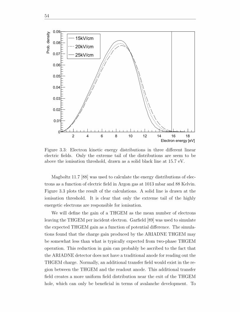
54
2 4 6 8 10 12 14 16 18Electron energy [eV]
0
0.01
0.02
0.03
0.04
0.05
0.06
0.07
0.08
0.09
Pro
b. d
ensi
ty
15kV/cm
20kV/cm
25kV/cm
Figure 3.3: Electron kinetic energy distributions in three different linearelectric fields. Only the extreme tail of the distributions are seem to beabove the ionisation threshold, drawn as a solid black line at 15.7 eV.
Magboltz 11.7 [88] was used to calculate the energy distributions of elec-
trons as a function of electric field in Argon gas at 1013 mbar and 88 Kelvin.
Figure 3.3 plots the result of the calculations. A solid line is drawn at the
ionisation threshold. It is clear that only the extreme tail of the highly
energetic electrons are responsible for ionisation.
We will define the gain of a THGEM as the mean number of electrons
leaving the THGEM per incident electron. Garfield [89] was used to simulate
the expected THGEM gain as a function of potential difference. The simula-
tions found that the charge gain produced by the ARIADNE THGEM may
be somewhat less than what is typically expected from two-phase THGEM
operation. This reduction in gain can probably be ascribed to the fact that
the ARIADNE detector does not have a traditional anode for reading out the
THGEM charge. Normally, an additional transfer field would exist in the re-
gion between the THGEM and the readout anode. This additional transfer
field creates a more uniform field distribution near the exit of the THGEM
hole, which can only be beneficial in terms of avalanche development. To
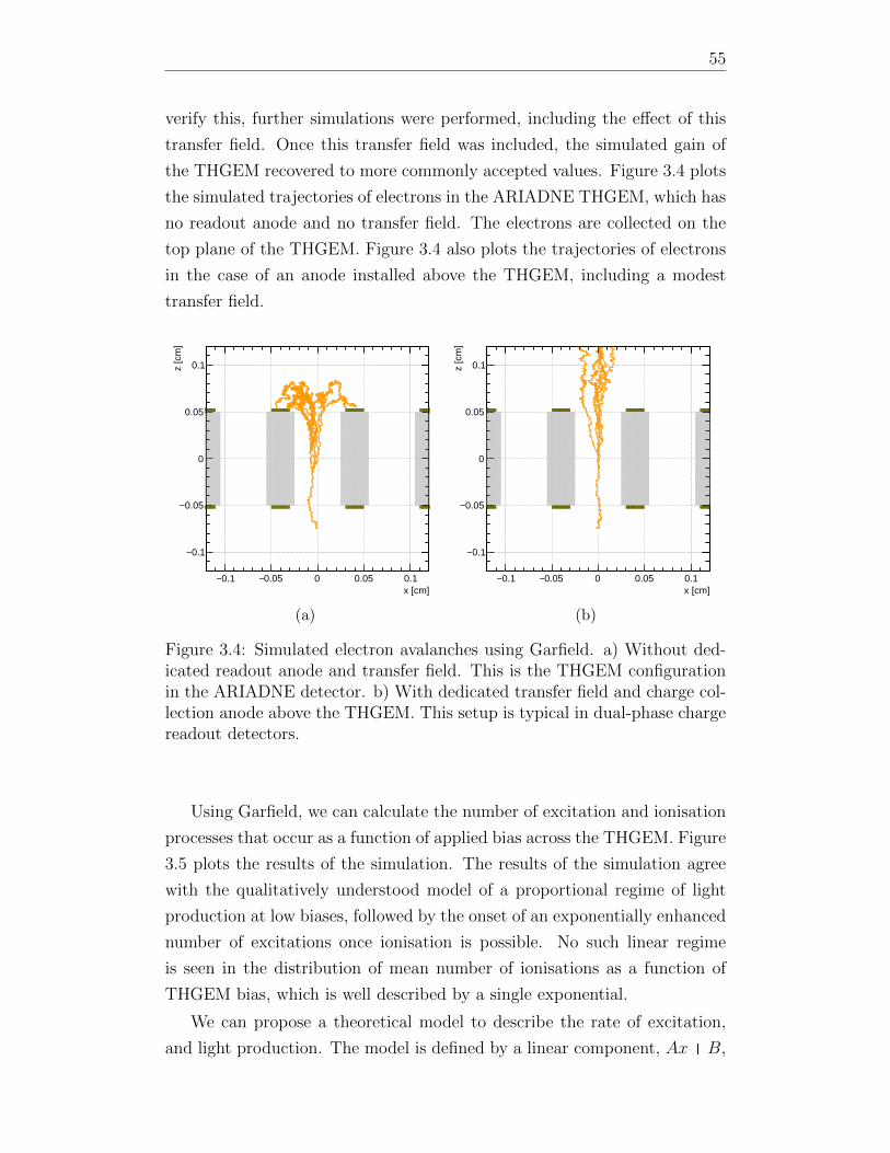
55
verify this, further simulations were performed, including the effect of this
transfer field. Once this transfer field was included, the simulated gain of
the THGEM recovered to more commonly accepted values. Figure 3.4 plots
the simulated trajectories of electrons in the ARIADNE THGEM, which has
no readout anode and no transfer field. The electrons are collected on the
top plane of the THGEM. Figure 3.4 also plots the trajectories of electrons
in the case of an anode installed above the THGEM, including a modest
transfer field.
0.1− 0.05− 0 0.05 0.1x [cm]
0.1−
0.05−
0
0.05
0.1z [c
m]
(a)
0.1− 0.05− 0 0.05 0.1x [cm]
0.1−
0.05−
0
0.05
0.1z [c
m]
(b)
Figure 3.4: Simulated electron avalanches using Garfield. a) Without ded-icated readout anode and transfer field. This is the THGEM configurationin the ARIADNE detector. b) With dedicated transfer field and charge col-lection anode above the THGEM. This setup is typical in dual-phase chargereadout detectors.
Using Garfield, we can calculate the number of excitation and ionisation
processes that occur as a function of applied bias across the THGEM. Figure
3.5 plots the results of the simulation. The results of the simulation agree
with the qualitatively understood model of a proportional regime of light
production at low biases, followed by the onset of an exponentially enhanced
number of excitations once ionisation is possible. No such linear regime
is seen in the distribution of mean number of ionisations as a function of
THGEM bias, which is well described by a single exponential.
We can propose a theoretical model to describe the rate of excitation,
and light production. The model is defined by a linear component, AxB,
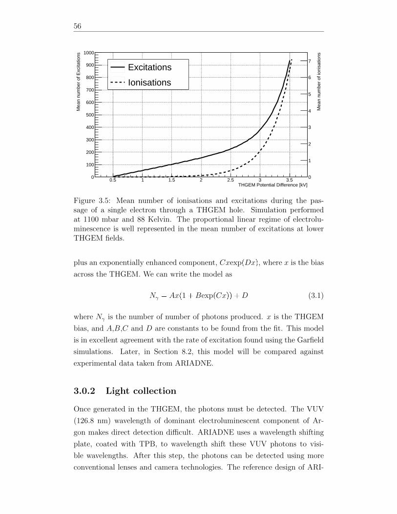
56
0.5 1 1.5 2 2.5 3 3.5THGEM Potential Difference [kV]
0
100
200
300
400
500
600
700
800
900
1000
Mea
n nu
mbe
r of
Exc
itatio
ns
0
1
2
3
4
5
6
7
Mea
n nu
mbe
r of
ioni
satio
ns
Excitations
Ionisations
Figure 3.5: Mean number of ionisations and excitations during the pas-sage of a single electron through a THGEM hole. Simulation performedat 1100 mbar and 88 Kelvin. The proportional linear regime of electrolu-minescence is well represented in the mean number of excitations at lowerTHGEM fields.
plus an exponentially enhanced component, CxexppDxq, where x is the bias
across the THGEM. We can write the model as
Nγ Axp1BexppCxqq D (3.1)
where Nγ is the number of number of photons produced. x is the THGEM
bias, and A,B,C and D are constants to be found from the fit. This model
is in excellent agreement with the rate of excitation found using the Garfield
simulations. Later, in Section 8.2, this model will be compared against
experimental data taken from ARIADNE.
3.0.2 Light collection
Once generated in the THGEM, the photons must be detected. The VUV
(126.8 nm) wavelength of dominant electroluminescent component of Ar-
gon makes direct detection difficult. ARIADNE uses a wavelength shifting
plate, coated with TPB, to wavelength shift these VUV photons to visi-
ble wavelengths. After this step, the photons can be detected using more
conventional lenses and camera technologies. The reference design of ARI-
57
ADNE uses four EMCCD cameras, each with a Spacecom VF50095M 50mm
focal length lens. The lens is installed at a distance of 1 m from the THGEM
plane. The VF50095M lens is a ’high speed’ lens, with n f-number of 0.95.
The f-number of lens is defined as
f-number fD (3.2)
where f is the focal length of the lens and D is the lens diameter. Thus, a
lower f-number translates to a larger aperture/diameter for the same focal
length. This larger aperture should increase the solid angle of the lens and
improve light collection. At a distance of 1 mm from the THGEM plane, and
with an aperture of 53 mm, the lens will have a solid angle of approximately
0.002 Steradian. This translates to an expected light collection efficiency of
0.016%.
The reference design of ARIADNE uses four Andor iXon Ultra 888 EM-
CCD cameras (see Section 4.8), which have a sensor size of 13.3 mm 13.3 mm.
The sensor has 1024 1024 pixels. When coupled with a 50mm focal length
lens, the resulting angle of view is approximately 15 degrees in both width
and height. Since the THGEM plane is 1 m away from the lens, the field of
view is slightly larger than 26 cm 26 cm per camera. The 1024 1024
pixels of the camera provide a nominal resolution of 260 µm 260 µm
per pixel. At this resolution, individual holes of the THGEM, which have
500 µm diameter, can be seen. Typically, the cameras are operated in 4 4
binning, producing a nominal resolution of slightly less than 1 mm per pixel.
Chapter 4
The ARIADNE detector
4.1 Detection principle
A general view of the ARIADNE detector can be seen in Figure 4.1. The
detection principle of the ARIADNE detector is illustrated in Figure 4.2.
Electrons are produced in the active volume during the passage of charged
particles. These electrons drift to the extraction region with a nominal
0.5 kV/cm drift field. The electrons are extracted into the gas phase using a
nominal 2 kV/cm extraction field. Once in the gas phase, the electrons enter
the holes of the THGEM, where light production occurs by electrolumines-
cence. This light is predominantly produced at 128 nm and is wavelength
shifted using TPB, coated on the underside of a borosilicate glass sheet
2 mm above the THGEM. The light that is re-emitted from the TPB, at
430 nm, is detected using four Andor EMCCD cameras. Since the cameras
are mounted outside of the cryogenic volume, they can be easily changed or
upgraded.
Four Hamamatsu R5912-02MOD PMTs are installed underneath the
TPC to provide detection of S1 light and auxiliary S2 light collection.
The design of ARIADNE was such that results from the detector should
be easy to interpret in the context of any future two-phase LArTPC designs.
The tiling of many 50 50 cm large electron multipliers (LEMs) is common
to many two-phase experiments and so this dimension was chosen for the
ARIADNE THGEM. The drift length of the TPC is mostly constrained by
logistics. The 80 cm drift length gives the detector a total height that may
still be easily manipulated using the locally available cranes.
58
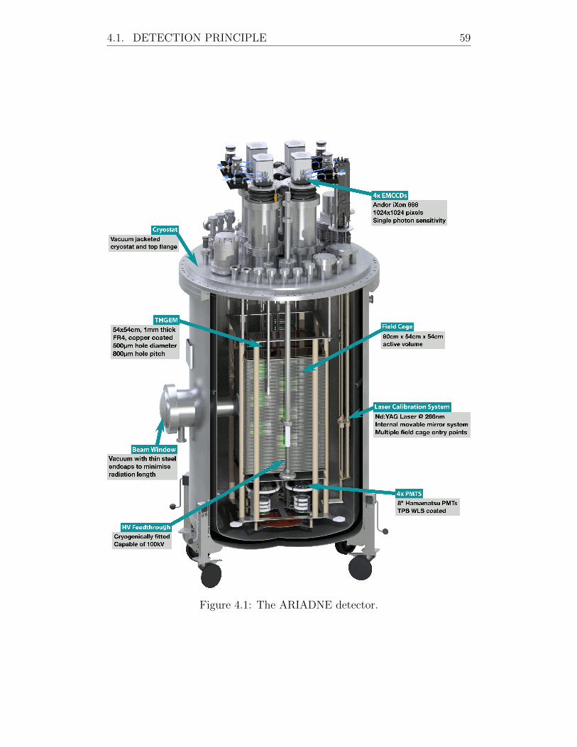
4.1. DETECTION PRINCIPLE 59
Figure 4.1: The ARIADNE detector.
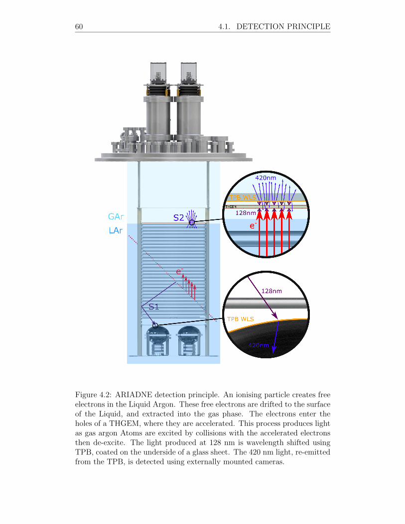
60 4.1. DETECTION PRINCIPLE
Figure 4.2: ARIADNE detection principle. An ionising particle creates freeelectrons in the Liquid Argon. These free electrons are drifted to the surfaceof the Liquid, and extracted into the gas phase. The electrons enter theholes of a THGEM, where they are accelerated. This process produces lightas gas argon Atoms are excited by collisions with the accelerated electronsthen de-excite. The light produced at 128 nm is wavelength shifted usingTPB, coated on the underside of a glass sheet. The 420 nm light, re-emittedfrom the TPB, is detected using externally mounted cameras.
4.2. CRYOSTAT 61
4.2 Cryostat
The ARIADNE cryostat is composed of two parts; a separable flange and
body. Both the cryostat flange and body have integral vacuum jackets
to minimise the total heat input into the detector volume. The cryostat
was manufactured by Wessington cryogenics, Tyne & Wear, UK. Figure 4.3
shows several photographs taken during manufacture of the cryostat. The
internal diameter of the cryostat is 1.07 meters and the internal height is
1.8 meters. The cryostat has a maximum rated capacity of 1530 litres when
95% full and a maximum service pressure of 4 bar(g).
4.2.1 Top flange
The top flange of the cryostat contains a wide selection of feedthroughs
for detector instrumentation. Four central DN200 flanges provide mounting
points for the cameras. The large diameter of these central feedthroughs
allow the cameras to have a wide field of view without being obscured. Two
DN160CF feedthroughs are provided in the top flange. A leybold Turbo-
vac 350i turbomolecular vacuum pump is directly attached to one of these
flanges. This direct attachment to the flange provides efficient pumping of
the detector volume. The detector volume is typically pumped to better than
1E-5 mbar before filling with Liquid Argon. This evacuation of the cryostat
helps to reduce outgassing of materials within the detector, reducing the
volume of impurities that must be handled by the liquid argon recirculation
and purification system.
Mounted to the second DN160CF feedthrough is a Cryomech AL300
Gifford-McMahon Cryorefrigerator unit. During operation, the ARIADNE
detector works as a closed loop. Thus, the heat loads of the cryostat must
be offset by this cold head. The cold head has a cooling capacity of 266 W
when at 80 K, reducing to 166 W at 50 K. This cooling capacity was found
to be sufficient for the head loads experienced by the cryostat, although
a cryocooler with increased cooling power may have been desirable. The
operation of the cryocooler is discussed in more detail in Section 4.11. A
DN75CF feedthrough provides a mounting point for the cathode high volt-
age feedthrough. This feedthrough is axially aligned with the toroid of the
TPC cathode, inside the cryostat. A large selection of auxiliary DN40CF
feedthroughs provide access for detector instrumentation such as thermo-
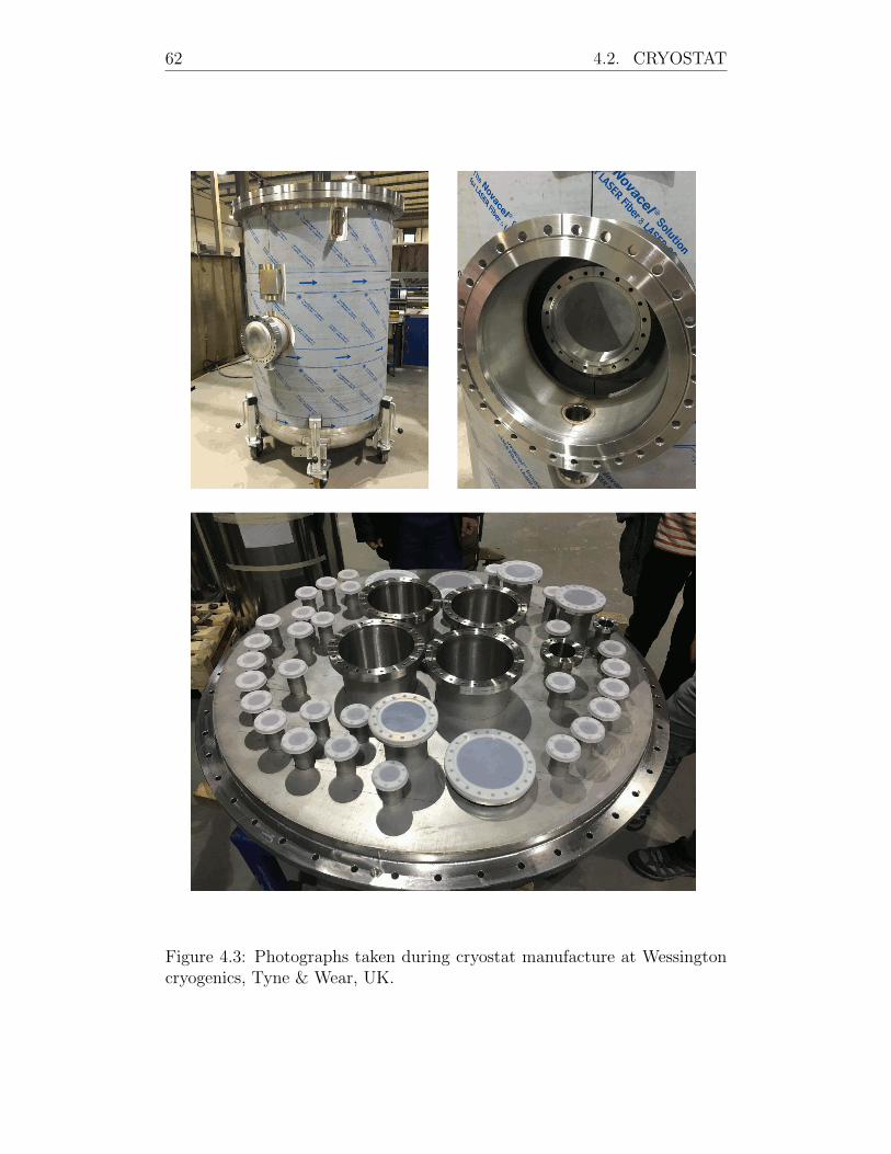
62 4.2. CRYOSTAT
Figure 4.3: Photographs taken during cryostat manufacture at Wessingtoncryogenics, Tyne & Wear, UK.
4.3. BEAM WINDOW 63
couples, cryogenic filling lines and pressure sensors.
4.2.2 Cryostat body
The cryostat body is vacuum jacket insulated vessel. The jacket of the
cryostat is fitted with multi-layer superinsulation. Six height-adjustable
wheels allow the height of the cryostat to be adjusted. This feature was
particularly useful during beamline operation where the height of the beam
window could be aligned with the height of the beamline. The inner wall of
the cryostat is fitted with a stiffening ring, which was necessary to allow the
cryostat volume to be pumped to UHV. Four lifting eyes allow the detector
to be lifted from the cryostat body. The cryostat was designed with an
indium groove to allow a vacuum tight seal to be created between the flange
and the main vessel. Typically during operation the vessel was instead
sealed using a Viton A gasket. This gasket is reusable, reducing the need
for expensive indium wire. In principle, Viton may allow the permeation of
small quantities of water through the bulk material. During operation the
detector is generally kept at a slight overpressure to minimise the change
of contamination through any microscopic leaks. It is expected that this
overpressure should result in a negligible rate of water permeation through
the Viton gasket.
4.3 Beam window
Two coaxial conflat flanges are integrated into the vacuum jacket of the
cryostat, providing mounting points for the beam window and beam plug
assemblies. The beam transport assembly is composed of two parts, an ex-
ternal beam window and an internal beam plug. The beam window forms
the interface between the air side of the detector and the vacuum jacket
of the cryostat. The beam plug forms the interface between the cryostat
and the liquid argon in the detector volume. Figure 4.4 shows a cross sec-
tion of the complete beam window assembly, when installed on the cryostat.
The design goals of the beam window are relatively simple; minimise the
total radiation length for thoroughgoing particles. The outer beam win-
dow, the interface between the air side and the cryostat, is formed from
0.9 mm thick stainless steel dished end. The shape of this window provides
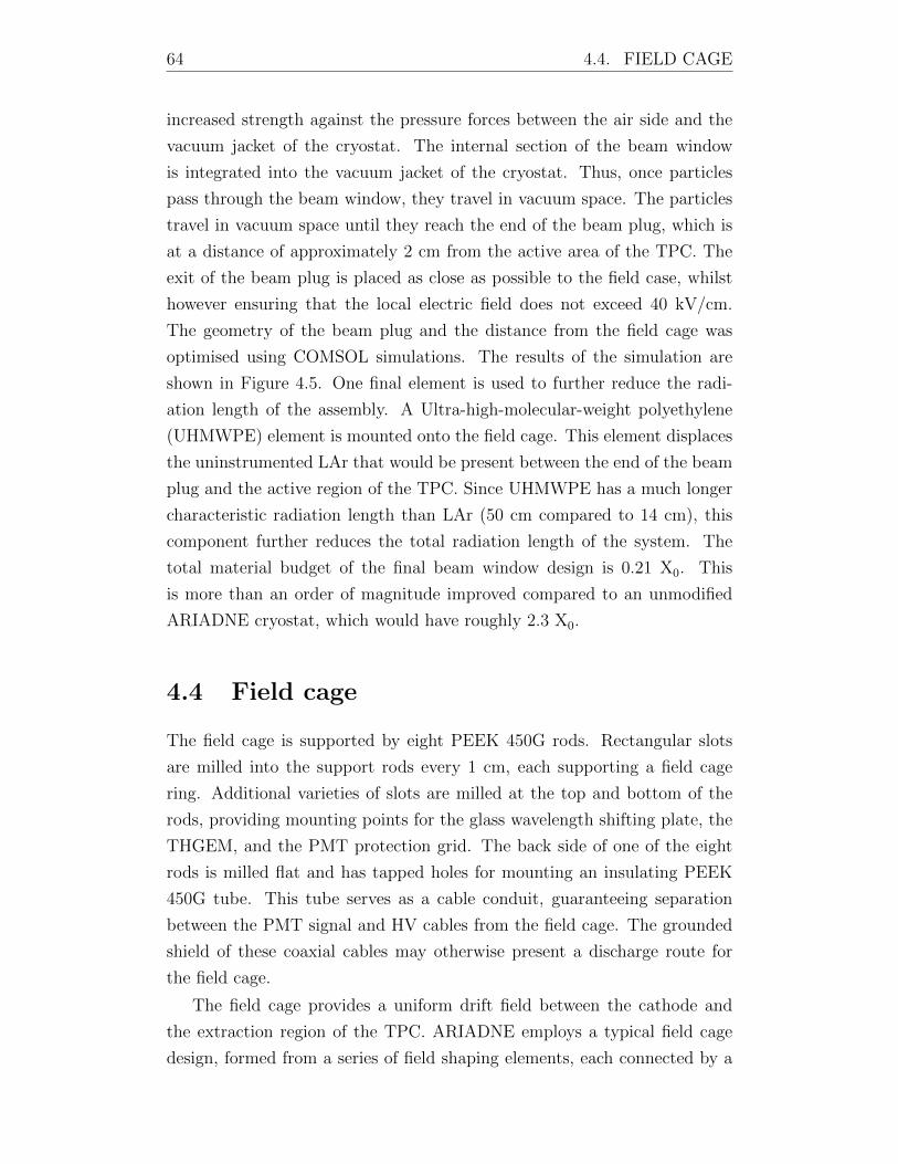
64 4.4. FIELD CAGE
increased strength against the pressure forces between the air side and the
vacuum jacket of the cryostat. The internal section of the beam window
is integrated into the vacuum jacket of the cryostat. Thus, once particles
pass through the beam window, they travel in vacuum space. The particles
travel in vacuum space until they reach the end of the beam plug, which is
at a distance of approximately 2 cm from the active area of the TPC. The
exit of the beam plug is placed as close as possible to the field case, whilst
however ensuring that the local electric field does not exceed 40 kV/cm.
The geometry of the beam plug and the distance from the field cage was
optimised using COMSOL simulations. The results of the simulation are
shown in Figure 4.5. One final element is used to further reduce the radi-
ation length of the assembly. A Ultra-high-molecular-weight polyethylene
(UHMWPE) element is mounted onto the field cage. This element displaces
the uninstrumented LAr that would be present between the end of the beam
plug and the active region of the TPC. Since UHMWPE has a much longer
characteristic radiation length than LAr (50 cm compared to 14 cm), this
component further reduces the total radiation length of the system. The
total material budget of the final beam window design is 0.21 X0. This
is more than an order of magnitude improved compared to an unmodified
ARIADNE cryostat, which would have roughly 2.3 X0.
4.4 Field cage
The field cage is supported by eight PEEK 450G rods. Rectangular slots
are milled into the support rods every 1 cm, each supporting a field cage
ring. Additional varieties of slots are milled at the top and bottom of the
rods, providing mounting points for the glass wavelength shifting plate, the
THGEM, and the PMT protection grid. The back side of one of the eight
rods is milled flat and has tapped holes for mounting an insulating PEEK
450G tube. This tube serves as a cable conduit, guaranteeing separation
between the PMT signal and HV cables from the field cage. The grounded
shield of these coaxial cables may otherwise present a discharge route for
the field cage.
The field cage provides a uniform drift field between the cathode and
the extraction region of the TPC. ARIADNE employs a typical field cage
design, formed from a series of field shaping elements, each connected by a
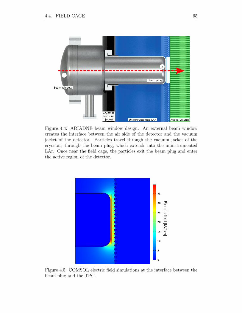
4.4. FIELD CAGE 65
Figure 4.4: ARIADNE beam window design. An external beam windowcreates the interface between the air side of the detector and the vacuumjacket of the detector. Particles travel through the vacuum jacket of thecryostat, through the beam plug, which extends into the uninstrumentedLAr. Once near the field cage, the particles exit the beam plug and enterthe active region of the detector.
Figure 4.5: COMSOL electric field simulations at the interface between thebeam plug and the TPC.
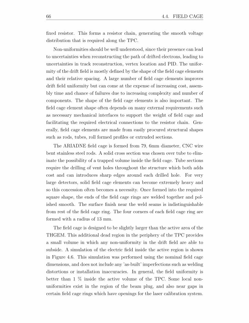
66 4.4. FIELD CAGE
fixed resistor. This forms a resistor chain, generating the smooth voltage
distribution that is required along the TPC.
Non-uniformities should be well understood, since their presence can lead
to uncertainties when reconstructing the path of drifted electrons, leading to
uncertainties in track reconstruction, vertex location and PID. The unifor-
mity of the drift field is mostly defined by the shape of the field cage elements
and their relative spacing. A large number of field cage elements improves
drift field uniformity but can come at the expense of increasing cost, assem-
bly time and chance of failures due to increasing complexity and number of
components. The shape of the field cage elements is also important. The
field cage element shape often depends on many external requirements such
as necessary mechanical interfaces to support the weight of field cage and
facilitating the required electrical connections to the resistor chain. Gen-
erally, field cage elements are made from easily procured structural shapes
such as rods, tubes, roll formed profiles or extruded sections.
The ARIADNE field cage is formed from 79, 6mm diameter, CNC wire
bent stainless steel rods. A solid cross section was chosen over tube to elim-
inate the possibility of a trapped volume inside the field cage. Tube sections
require the drilling of vent holes throughout the structure which both adds
cost and can introduces sharp edges around each drilled hole. For very
large detectors, solid field cage elements can become extremely heavy and
so this concession often becomes a necessity. Once formed into the required
square shape, the ends of the field cage rings are welded together and pol-
ished smooth. The surface finish near the weld seams is indistinguishable
from rest of the field cage ring. The four corners of each field cage ring are
formed with a radius of 13 mm.
The field cage is designed to be slightly larger than the active area of the
THGEM. This additional dead region in the periphery of the TPC provides
a small volume in which any non-uniformity in the drift field are able to
subside. A simulation of the electric field inside the active region is shown
in Figure 4.6. This simulation was performed using the nominal field cage
dimensions, and does not include any ’as-built’ imperfections such as welding
distortions or installation inaccuracies. In general, the field uniformity is
better than 1 % inside the active volume of the TPC. Some local non-
uniformities exist in the region of the beam plug, and also near gaps in
certain field cage rings which have openings for the laser calibration system.
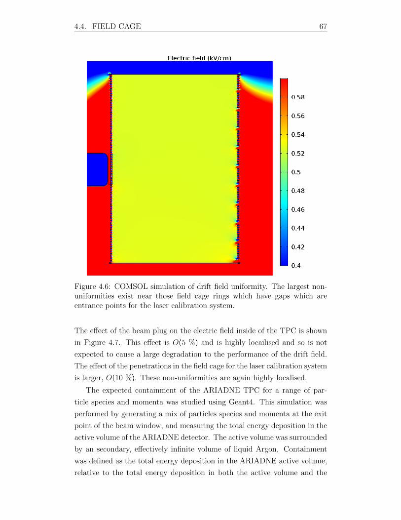
4.4. FIELD CAGE 67
Figure 4.6: COMSOL simulation of drift field uniformity. The largest non-uniformities exist near those field cage rings which have gaps which areentrance points for the laser calibration system.
The effect of the beam plug on the electric field inside of the TPC is shown
in Figure 4.7. This effect is Op5 %q and is highly locailised and so is not
expected to cause a large degradation to the performance of the drift field.
The effect of the penetrations in the field cage for the laser calibration system
is larger, Op10 %q. These non-uniformities are again highly localised.
The expected containment of the ARIADNE TPC for a range of par-
ticle species and momenta was studied using Geant4. This simulation was
performed by generating a mix of particles species and momenta at the exit
point of the beam window, and measuring the total energy deposition in the
active volume of the ARIADNE detector. The active volume was surrounded
by an secondary, effectively infinite volume of liquid Argon. Containment
was defined as the total energy deposition in the ARIADNE active volume,
relative to the total energy deposition in both the active volume and the
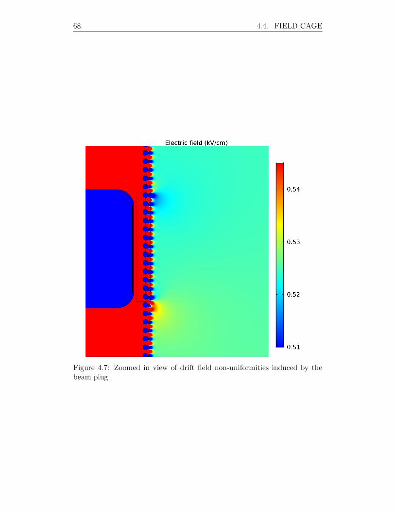
68 4.4. FIELD CAGE
Figure 4.7: Zoomed in view of drift field non-uniformities induced by thebeam plug.
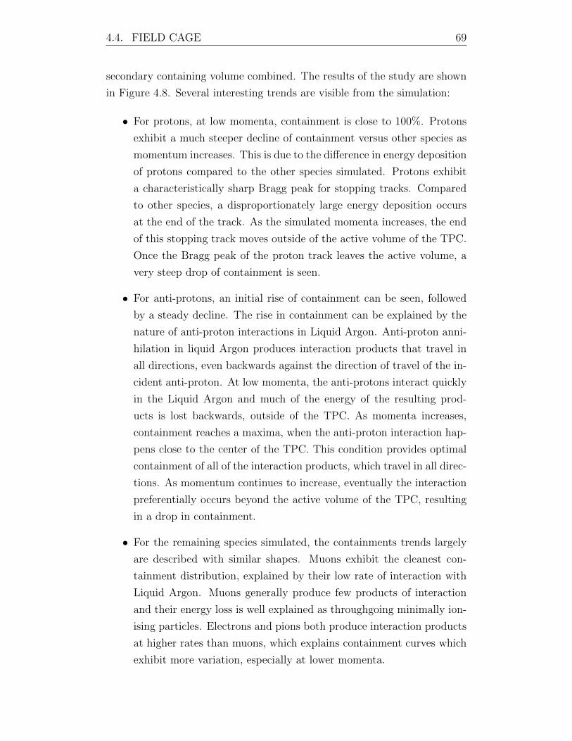
4.4. FIELD CAGE 69
secondary containing volume combined. The results of the study are shown
in Figure 4.8. Several interesting trends are visible from the simulation:
• For protons, at low momenta, containment is close to 100%. Protons
exhibit a much steeper decline of containment versus other species as
momentum increases. This is due to the difference in energy deposition
of protons compared to the other species simulated. Protons exhibit
a characteristically sharp Bragg peak for stopping tracks. Compared
to other species, a disproportionately large energy deposition occurs
at the end of the track. As the simulated momenta increases, the end
of this stopping track moves outside of the active volume of the TPC.
Once the Bragg peak of the proton track leaves the active volume, a
very steep drop of containment is seen.
• For anti-protons, an initial rise of containment can be seen, followed
by a steady decline. The rise in containment can be explained by the
nature of anti-proton interactions in Liquid Argon. Anti-proton anni-
hilation in liquid Argon produces interaction products that travel in
all directions, even backwards against the direction of travel of the in-
cident anti-proton. At low momenta, the anti-protons interact quickly
in the Liquid Argon and much of the energy of the resulting prod-
ucts is lost backwards, outside of the TPC. As momenta increases,
containment reaches a maxima, when the anti-proton interaction hap-
pens close to the center of the TPC. This condition provides optimal
containment of all of the interaction products, which travel in all direc-
tions. As momentum continues to increase, eventually the interaction
preferentially occurs beyond the active volume of the TPC, resulting
in a drop in containment.
• For the remaining species simulated, the containments trends largely
are described with similar shapes. Muons exhibit the cleanest con-
tainment distribution, explained by their low rate of interaction with
Liquid Argon. Muons generally produce few products of interaction
and their energy loss is well explained as throughgoing minimally ion-
ising particles. Electrons and pions both produce interaction products
at higher rates than muons, which explains containment curves which
exhibit more variation, especially at lower momenta.
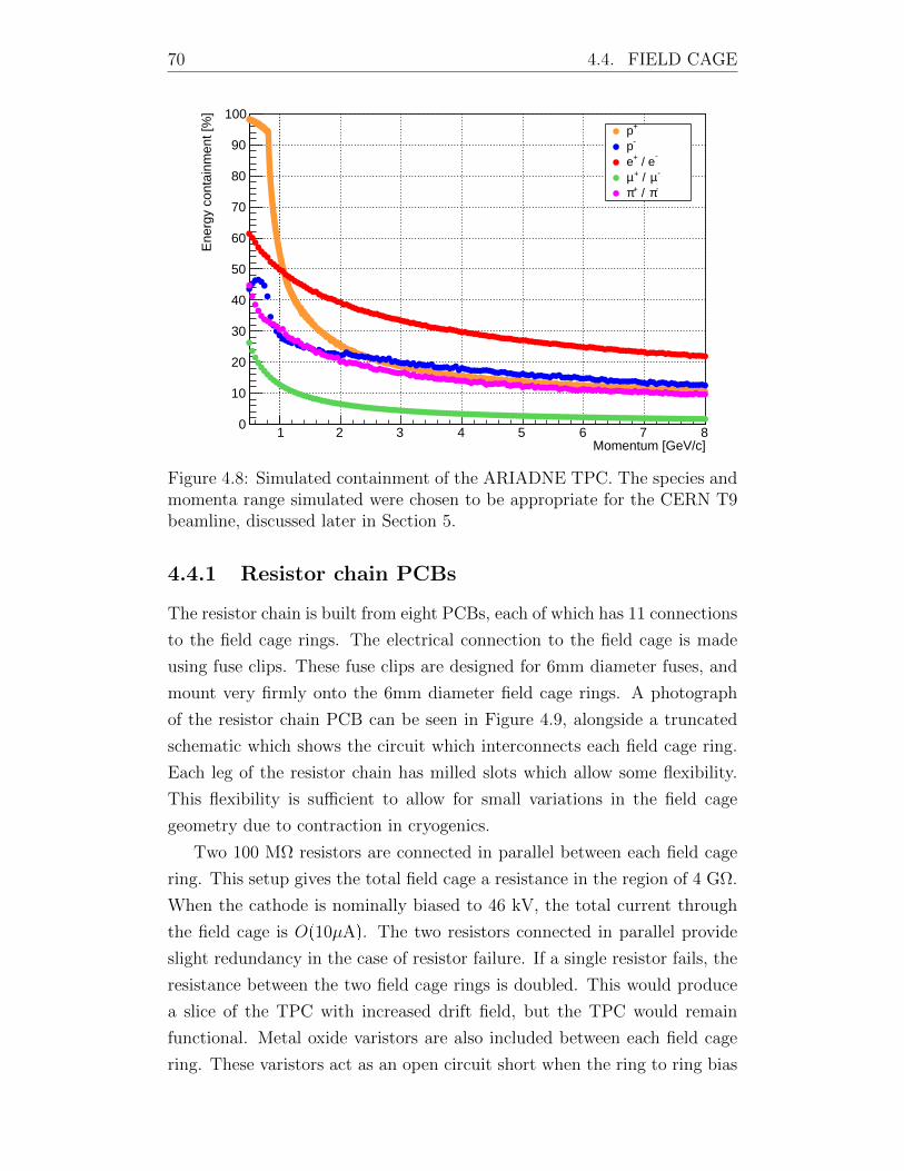
70 4.4. FIELD CAGE
1 2 3 4 5 6 7 8Momentum [GeV/c]
0
10
20
30
40
50
60
70
80
90
100
Ene
rgy
cont
ainm
ent [
%]
+p-p
- / e+e
-µ / +µ-π / +π
Figure 4.8: Simulated containment of the ARIADNE TPC. The species andmomenta range simulated were chosen to be appropriate for the CERN T9beamline, discussed later in Section 5.
4.4.1 Resistor chain PCBs
The resistor chain is built from eight PCBs, each of which has 11 connections
to the field cage rings. The electrical connection to the field cage is made
using fuse clips. These fuse clips are designed for 6mm diameter fuses, and
mount very firmly onto the 6mm diameter field cage rings. A photograph
of the resistor chain PCB can be seen in Figure 4.9, alongside a truncated
schematic which shows the circuit which interconnects each field cage ring.
Each leg of the resistor chain has milled slots which allow some flexibility.
This flexibility is sufficient to allow for small variations in the field cage
geometry due to contraction in cryogenics.
Two 100 MΩ resistors are connected in parallel between each field cage
ring. This setup gives the total field cage a resistance in the region of 4 GΩ.
When the cathode is nominally biased to 46 kV, the total current through
the field cage is Op10µAq. The two resistors connected in parallel provide
slight redundancy in the case of resistor failure. If a single resistor fails, the
resistance between the two field cage rings is doubled. This would produce
a slice of the TPC with increased drift field, but the TPC would remain
functional. Metal oxide varistors are also included between each field cage
ring. These varistors act as an open circuit short when the ring to ring bias
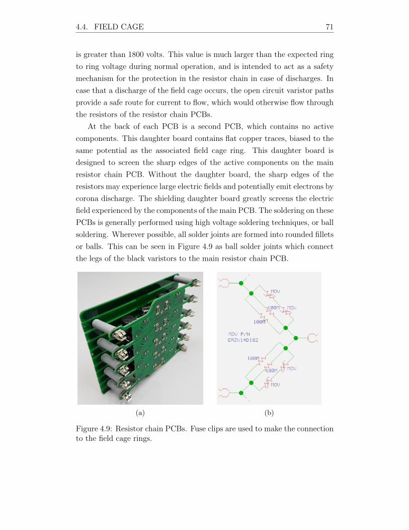
4.4. FIELD CAGE 71
is greater than 1800 volts. This value is much larger than the expected ring
to ring voltage during normal operation, and is intended to act as a safety
mechanism for the protection in the resistor chain in case of discharges. In
case that a discharge of the field cage occurs, the open circuit varistor paths
provide a safe route for current to flow, which would otherwise flow through
the resistors of the resistor chain PCBs.
At the back of each PCB is a second PCB, which contains no active
components. This daughter board contains flat copper traces, biased to the
same potential as the associated field cage ring. This daughter board is
designed to screen the sharp edges of the active components on the main
resistor chain PCB. Without the daughter board, the sharp edges of the
resistors may experience large electric fields and potentially emit electrons by
corona discharge. The shielding daughter board greatly screens the electric
field experienced by the components of the main PCB. The soldering on these
PCBs is generally performed using high voltage soldering techniques, or ball
soldering. Wherever possible, all solder joints are formed into rounded fillets
or balls. This can be seen in Figure 4.9 as ball solder joints which connect
the legs of the black varistors to the main resistor chain PCB.
(a) (b)
Figure 4.9: Resistor chain PCBs. Fuse clips are used to make the connectionto the field cage rings.
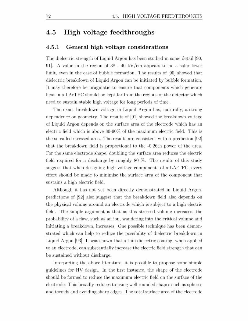
72 4.5. HIGH VOLTAGE FEEDTHROUGHS
4.5 High voltage feedthroughs
4.5.1 General high voltage considerations
The dielectric strength of Liquid Argon has been studied in some detail [90,
91]. A value in the region of 38 - 40 kV/cm appears to be a safer lower
limit, even in the case of bubble formation. The results of [90] showed that
dielectric breakdown of Liquid Argon can be initiated by bubble formation.
It may therefore be pragmatic to ensure that components which generate
heat in a LArTPC should be kept far from the regions of the detector which
need to sustain stable high voltage for long periods of time.
The exact breakdown voltage in Liquid Argon has, naturally, a strong
dependence on geometry. The results of [91] showed the breakdown voltage
of Liquid Argon depends on the surface area of the electrode which has an
electric field which is above 80-90% of the maximum electric field. This is
the so called stressed area. The results are consistent with a prediction [92]
that the breakdown field is proportional to the -0.26th power of the area.
For the same electrode shape, doubling the surface area reduces the electric
field required for a discharge by roughly 80 %. The results of this study
suggest that when designing high voltage components of a LArTPC, every
effort should be made to minimise the surface area of the component that
sustains a high electric field.
Although it has not yet been directly demonstrated in Liquid Argon,
predictions of [92] also suggest that the breakdown field also depends on
the physical volume around an electrode which is subject to a high electric
field. The simple argument is that as this stressed volume increases, the
probability of a flaw, such as an ion, wandering into the critical volume and
initiating a breakdown, increases. One possible technique has been demon-
strated which can help to reduce the possibility of dielectric breakdown in
Liquid Argon [93]. It was shown that a thin dielectric coating, when applied
to an electrode, can substantially increase the electric field strength that can
be sustained without discharge.
Interpreting the above literature, it is possible to propose some simple
guidelines for HV design. In the first instance, the shape of the electrode
should be formed to reduce the maximum electric field on the surface of the
electrode. This broadly reduces to using well rounded shapes such as spheres
and toroids and avoiding sharp edges. The total surface area of the electrode
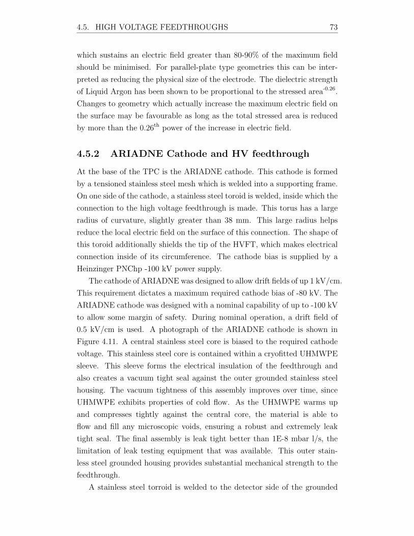
4.5. HIGH VOLTAGE FEEDTHROUGHS 73
which sustains an electric field greater than 80-90% of the maximum field
should be minimised. For parallel-plate type geometries this can be inter-
preted as reducing the physical size of the electrode. The dielectric strength
of Liquid Argon has been shown to be proportional to the stressed area-0.26.
Changes to geometry which actually increase the maximum electric field on
the surface may be favourable as long as the total stressed area is reduced
by more than the 0.26th power of the increase in electric field.
4.5.2 ARIADNE Cathode and HV feedthrough
At the base of the TPC is the ARIADNE cathode. This cathode is formed
by a tensioned stainless steel mesh which is welded into a supporting frame.
On one side of the cathode, a stainless steel toroid is welded, inside which the
connection to the high voltage feedthrough is made. This torus has a large
radius of curvature, slightly greater than 38 mm. This large radius helps
reduce the local electric field on the surface of this connection. The shape of
this toroid additionally shields the tip of the HVFT, which makes electrical
connection inside of its circumference. The cathode bias is supplied by a
Heinzinger PNChp -100 kV power supply.
The cathode of ARIADNE was designed to allow drift fields of up 1 kV/cm.
This requirement dictates a maximum required cathode bias of -80 kV. The
ARIADNE cathode was designed with a nominal capability of up to -100 kV
to allow some margin of safety. During nominal operation, a drift field of
0.5 kV/cm is used. A photograph of the ARIADNE cathode is shown in
Figure 4.11. A central stainless steel core is biased to the required cathode
voltage. This stainless steel core is contained within a cryofitted UHMWPE
sleeve. This sleeve forms the electrical insulation of the feedthrough and
also creates a vacuum tight seal against the outer grounded stainless steel
housing. The vacuum tightness of this assembly improves over time, since
UHMWPE exhibits properties of cold flow. As the UHMWPE warms up
and compresses tightly against the central core, the material is able to
flow and fill any microscopic voids, ensuring a robust and extremely leak
tight seal. The final assembly is leak tight better than 1E-8 mbar l/s, the
limitation of leak testing equipment that was available. This outer stain-
less steel grounded housing provides substantial mechanical strength to the
feedthrough.
A stainless steel torroid is welded to the detector side of the grounded
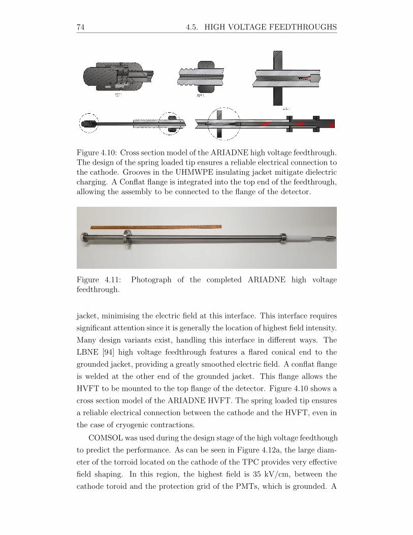
74 4.5. HIGH VOLTAGE FEEDTHROUGHS
Figure 4.10: Cross section model of the ARIADNE high voltage feedthrough.The design of the spring loaded tip ensures a reliable electrical connection tothe cathode. Grooves in the UHMWPE insulating jacket mitigate dielectriccharging. A Conflat flange is integrated into the top end of the feedthrough,allowing the assembly to be connected to the flange of the detector.
Figure 4.11: Photograph of the completed ARIADNE high voltagefeedthrough.
jacket, minimising the electric field at this interface. This interface requires
significant attention since it is generally the location of highest field intensity.
Many design variants exist, handling this interface in different ways. The
LBNE [94] high voltage feedthrough features a flared conical end to the
grounded jacket, providing a greatly smoothed electric field. A conflat flange
is welded at the other end of the grounded jacket. This flange allows the
HVFT to be mounted to the top flange of the detector. Figure 4.10 shows a
cross section model of the ARIADNE HVFT. The spring loaded tip ensures
a reliable electrical connection between the cathode and the HVFT, even in
the case of cryogenic contractions.
COMSOL was used during the design stage of the high voltage feedthough
to predict the performance. As can be seen in Figure 4.12a, the large diam-
eter of the torroid located on the cathode of the TPC provides very effective
field shaping. In this region, the highest field is 35 kV/cm, between the
cathode toroid and the protection grid of the PMTs, which is grounded. A
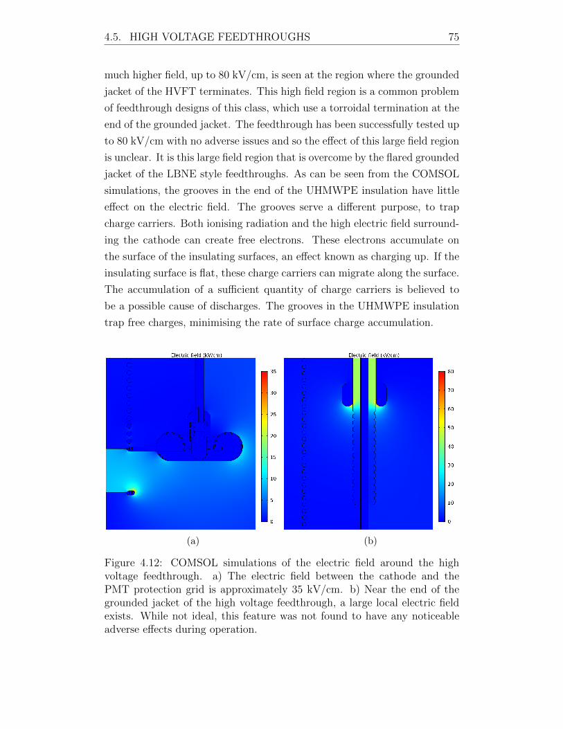
4.5. HIGH VOLTAGE FEEDTHROUGHS 75
much higher field, up to 80 kV/cm, is seen at the region where the grounded
jacket of the HVFT terminates. This high field region is a common problem
of feedthrough designs of this class, which use a torroidal termination at the
end of the grounded jacket. The feedthrough has been successfully tested up
to 80 kV/cm with no adverse issues and so the effect of this large field region
is unclear. It is this large field region that is overcome by the flared grounded
jacket of the LBNE style feedthroughs. As can be seen from the COMSOL
simulations, the grooves in the end of the UHMWPE insulation have little
effect on the electric field. The grooves serve a different purpose, to trap
charge carriers. Both ionising radiation and the high electric field surround-
ing the cathode can create free electrons. These electrons accumulate on
the surface of the insulating surfaces, an effect known as charging up. If the
insulating surface is flat, these charge carriers can migrate along the surface.
The accumulation of a sufficient quantity of charge carriers is believed to
be a possible cause of discharges. The grooves in the UHMWPE insulation
trap free charges, minimising the rate of surface charge accumulation.
(a) (b)
Figure 4.12: COMSOL simulations of the electric field around the highvoltage feedthrough. a) The electric field between the cathode and thePMT protection grid is approximately 35 kV/cm. b) Near the end of thegrounded jacket of the high voltage feedthrough, a large local electric fieldexists. While not ideal, this feature was not found to have any noticeableadverse effects during operation.
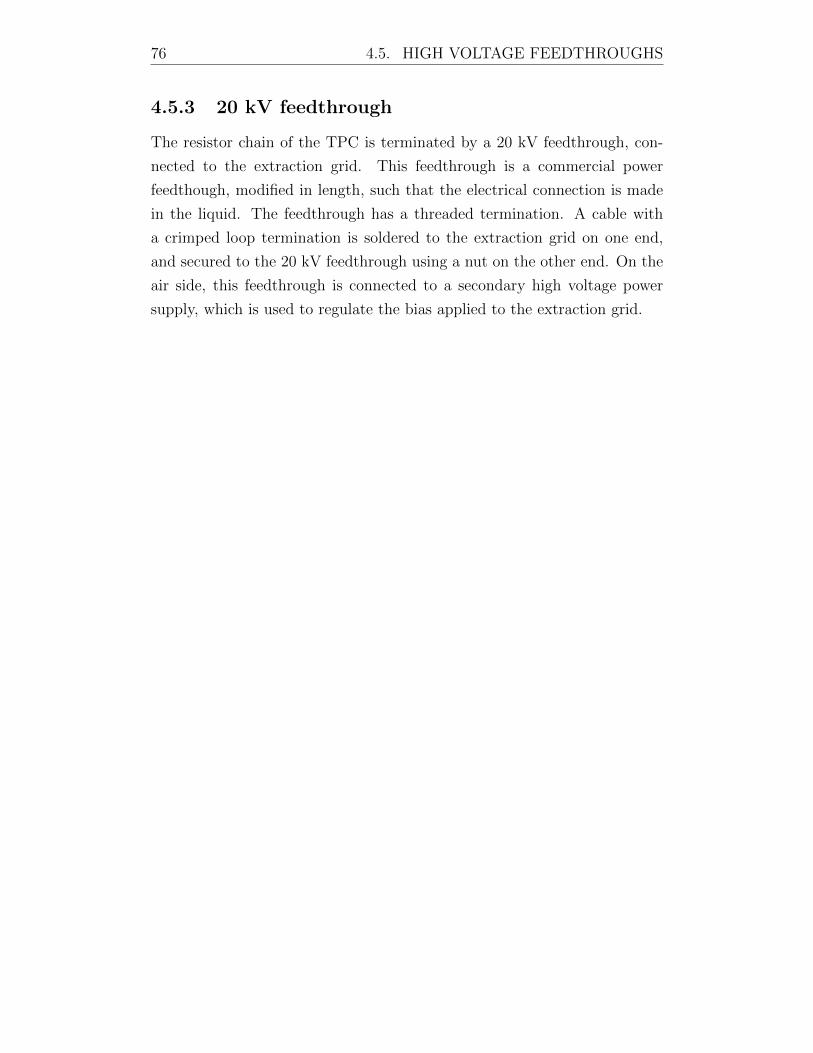
76 4.5. HIGH VOLTAGE FEEDTHROUGHS
4.5.3 20 kV feedthrough
The resistor chain of the TPC is terminated by a 20 kV feedthrough, con-
nected to the extraction grid. This feedthrough is a commercial power
feedthough, modified in length, such that the electrical connection is made
in the liquid. The feedthrough has a threaded termination. A cable with
a crimped loop termination is soldered to the extraction grid on one end,
and secured to the 20 kV feedthrough using a nut on the other end. On the
air side, this feedthrough is connected to a secondary high voltage power
supply, which is used to regulate the bias applied to the extraction grid.
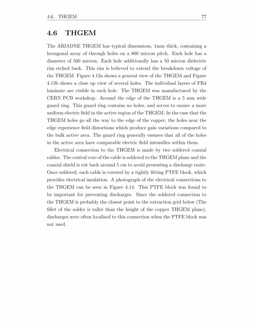
4.6. THGEM 77
4.6 THGEM
The ARIADNE THGEM has typical dimensions, 1mm thick, containing a
hexagonal array of through holes on a 800 micron pitch. Each hole has a
diameter of 500 micron. Each hole additionally has a 50 micron dielectric
rim etched back. This rim is believed to extend the breakdown voltage of
the THGEM. Figure 4.13a shows a general view of the THGEM and Figure
4.13b shows a close up view of several holes. The individual layers of FR4
laminate are visible in each hole. The THGEM was manufactured by the
CERN PCB workshop. Around the edge of the THGEM is a 5 mm wide
guard ring. This guard ring contains no holes, and serves to ensure a more
uniform electric field in the active region of the THGEM. In the case that the
THGEM holes go all the way to the edge of the copper, the holes near the
edge experience field distortions which produce gain variations compared to
the bulk active area. The guard ring generally ensures that all of the holes
in the active area have comparable electric field intensifies within them.
Electrical connection to the THGEM is made by two soldered coaxial
cables. The central core of the cable is soldered to the THGEM plane and the
coaxial shield is cut back around 5 cm to avoid presenting a discharge route.
Once soldered, each cable is covered by a tightly fitting PTFE block, which
provides electrical insulation. A photograph of the electrical connections to
the THGEM can be seen in Figure 4.14. This PTFE block was found to
be important for preventing discharges. Since the soldered connection to
the THGEM is probably the closest point to the extraction grid below (The
fillet of the solder is taller than the height of the copper THGEM plane),
discharges were often localised to this connection when the PTFE block was
not used.
78 4.6. THGEM
(a) (b)
Figure 4.13: The ARIADNE THGEM. a) A general overview of theTHGEM. The active area is 53 cm 53 cm. b) A close up view of individualholes in the THGEM. The individual FR4 laminate layers are visible insideeach hole. The dielectric rim around each hole can also be seen.
Figure 4.14: A close up view of the PTFE connector blocks, used to insulatethe electrical connection to the THGEM. A cable is soldered to the THGEM,and then the PTFE blocks are installed with a light press fit, encapsulatingthe solder fillet.
4.7. GLASS SHEET / WAVELENGTH SHIFTING 79
4.7 Glass sheet / wavelength shifting
The light released from the THGEM in Argon is at 128 nm. For now, this
light cannot be detected directly. TPB is used to wavelength shift the 128 nm
light to 420 nm. 420 nm can be detected with good quantum efficiency by
the EMCCD cameras. To perform this wavelength shifting, a 2.75mm thick
borofloat glass sheet, with a finish of 60/40 scratch/dig is coated on the
underside with TPB. The sheet is installed 1.8 mm above the THGEM.
The distance between the THGEM and the TPB was found to have some
influence on tracking resolution - this is discussed further in Section 9.1.3.
The nominal coating thickness was 0.05 mgcm2.
The coating was performed by vacuum evaporation, using a custom-built
vacuum evaporation chamber. The chamber uses five crucibles to increasing
coating uniformity. A model of the vacuum evaporation chamber is shown
in Figure 4.15. The chamber was evacuated to better than 1E-4 mbar before
the coating process is started. Once a good vacuum is achieved, current is
supplied to the crucibles, causing them to heat up. The current supplied
to each crucible is gradually increased until the TPB within each crucible
evaporates and coats the underside of the glass, which is suspended above.
The coating thickness is controlled by adjusting both the ammount of TPB
contained within each crucible and the distance between the crucibles and
the glass sheet. A viewport on the side of the vacuum chamber provides
access to visually inspect the coating process and to check that all of the
crucibles have successfully evaporated the TPB. Once the coating is com-
plete, the glass sheet is generally stored in the vacuum chamber for as long
as possible. Once the detector is ready to close, the glass sheet is removed
from the chamber and installed in the detector. This process attempts to
minimise the amount of time which the TPB is exposed to ambient light,
since TPB is known to deteriorate by exposure.
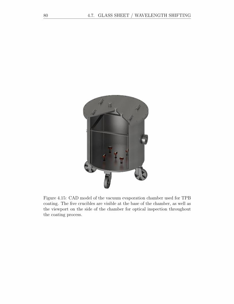
80 4.7. GLASS SHEET / WAVELENGTH SHIFTING
Figure 4.15: CAD model of the vacuum evaporation chamber used for TPBcoating. The five crucibles are visible at the base of the chamber, as well asthe viewport on the side of the chamber for optical inspection throughoutthe coating process.
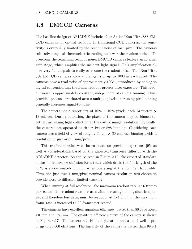
4.8. EMCCD CAMERAS 81
4.8 EMCCD Cameras
The baseline design of ARIADNE includes four Andor iXon Ultra 888 EM-
CCD cameras for optical readout. In traditional CCD cameras, the sensi-
tivity is eventually limited by the readout noise of each pixel. The cameras
take advantage of thermoelectric cooling to lower the readout noise. To
overcome the remaining readout noise, EMCCD cameras feature an internal
gain stage, which amplifies the incident light signal. This amplification al-
lows very faint signals to easily overcome the readout noise. The iXon Ultra
888 EMCCD cameras allow signal gains of up to 1000 in each pixel. The
cameras have a read noise of approximately 100e, introduced by analog to
digital conversion and the frame readout process after exposure. This read-
out noise is approximately constant, independent of camera binning. Thus,
provided photons are shared across multiple pixels, increasing pixel binning
generally increases signal-to-noise.
The camera has a sensor size of 1024 1024 pixels, each 13 micron 13 micron. During operation, the pixels of the camera may be binned to-
gether, increasing light collection at the cost of image resolution. Typically,
the cameras are operated at either 4x4 or 8x8 binning. Considering each
camera has a field of view of roughly 30 cm 30 cm, 4x4 binning yields a
resolution of just over 1 mm/pixel.
This resolution value was chosen based on previous experience [95] as
well as considerations based on the expected transverse diffusion with the
ARIADNE detector. As can be seen in Figure 2.10, the expected standard
deviation transverse diffusion for a track which drifts the full length of the
TPC is approximately 1.1 mm when operating at the nominal drift fields.
Thus, the just over 1 mm/pixel nominal camera resolution was chosen to
provide close to diffusion limited tracking.
When running at full resolution, the maximum readout rate is 26 frames
per second. The readout rate increases with increasing binning since less pix-
els, and therefore less data, must be readout. At 4x4 binning, the maximum
frame rate is increased to 92 frames per second.
The cameras have excellent quantum efficiency, better than 80 % between
410 nm and 780 nm. The quantum efficiency curve of the camera is shown
in Figure 4.17. The camera has 16-bit digitisation and a pixel well depth
of up to 80,000 electrons. The linearity of the camera is better than 99.9%
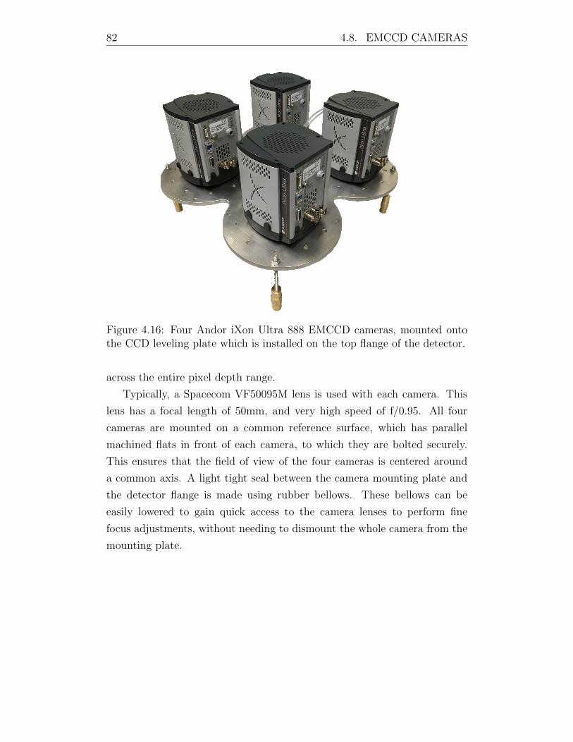
82 4.8. EMCCD CAMERAS
Figure 4.16: Four Andor iXon Ultra 888 EMCCD cameras, mounted ontothe CCD leveling plate which is installed on the top flange of the detector.
across the entire pixel depth range.
Typically, a Spacecom VF50095M lens is used with each camera. This
lens has a focal length of 50mm, and very high speed of f/0.95. All four
cameras are mounted on a common reference surface, which has parallel
machined flats in front of each camera, to which they are bolted securely.
This ensures that the field of view of the four cameras is centered around
a common axis. A light tight seal between the camera mounting plate and
the detector flange is made using rubber bellows. These bellows can be
easily lowered to gain quick access to the camera lenses to perform fine
focus adjustments, without needing to dismount the whole camera from the
mounting plate.
4.8. EMCCD CAMERAS 83
0
10
20
30
40
50
60
70
80
90
100
200 300 400 500 600 700 800 900 1000 1100 1200
Quan
tum
eff
icie
ncy
(%)
Wavelength (nm)
Figure 4.17: Quantum efficiency curve of the Andor iXon Ultra 888 EM-CCD cameras, compared to the emission spectrum of TPB. TPB emissionspectrum reproduced from [96].
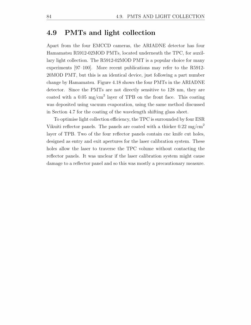
84 4.9. PMTS AND LIGHT COLLECTION
4.9 PMTs and light collection
Apart from the four EMCCD cameras, the ARIADNE detector has four
Hamamatsu R5912-02MOD PMTs, located underneath the TPC, for auxil-
lary light collection. The R5912-02MOD PMT is a popular choice for many
experiments [97–100]. More recent publications may refer to the R5912-
20MOD PMT, but this is an identical device, just following a part number
change by Hamamatsu. Figure 4.18 shows the four PMTs in the ARIADNE
detector. Since the PMTs are not directly sensitive to 128 nm, they are
coated with a 0.05 mgcm2 layer of TPB on the front face. This coating
was deposited using vacuum evaporation, using the same method discussed
in Section 4.7 for the coating of the wavelength shifting glass sheet.
To optimise light collection efficiency, the TPC is surrounded by four ESR
Vikuiti reflector panels. The panels are coated with a thicker 0.22 mgcm2
layer of TPB. Two of the four reflector panels contain cnc knife cut holes,
designed as entry and exit apertures for the laser calibration system. These
holes allow the laser to traverse the TPC volume without contacting the
reflector panels. It was unclear if the laser calibration system might cause
damage to a reflector panel and so this was mostly a precautionary measure.
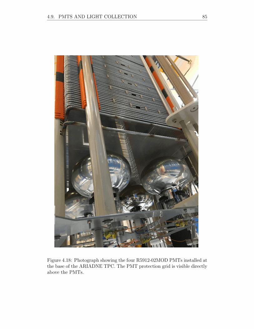
4.9. PMTS AND LIGHT COLLECTION 85
Figure 4.18: Photograph showing the four R5912-02MOD PMTs installed atthe base of the ARIADNE TPC. The PMT protection grid is visible directlyabove the PMTs.
86 4.9. PMTS AND LIGHT COLLECTION
(a) (b)
Figure 4.19: ARIADNE reflector panels. a) the inside face of each reflectorpanel is coated with a 0.22 mgcm2 layer of TPB. b) The reflector panelsinstalled onto the TPC. Holes in certain reflector panels are provided asaccess points for the laser calibration system. The UHMWPE block, thatfills the interface between the beam plug and the TPC, is also visible.
4.10. LIQUID ARGON PURIFICATION AND RECIRCULATION 87
4.10 Liquid Argon purification and recircu-
lation
As we saw in Sections 2.4.1 and 2.5.3, Liquid argon purity is critical. The
purity determines both the maximum drift distance in the TPC as well
as the scintillation light yield. Control over electronegative impurities in
particular is especially important. Electronegative impurities preferentially
attach to drifting electrons, absorbing the detector signal. The purpose of
the recirculation/filtration system in a liquid argon TPC is to remove those
impurities which may degrade detector performance.
4.10.1 Liquid argon Purification cartridge
In the case of ARIADNE, an external purification system would greatly
complicate cryostat design. It was decided that an internal system was a
more practical option. An internal recirculation system promises minimal
heat losses since the liquid argon is recirculated within a single cryostat.
Obvious drawbacks however are the difficulty of accessing the system in
case of any problems. The difficulty of access to the recirculation system
for maintenance places tough constraints on the design. The system has
to be designed for reliable, maintenance-free operation for extended periods
of time. These constraints favour a design that is mechanically simple.
Difficulty of access also means that before detector filling, the recirculation
system must be fully regenerated. The filtration system cannot be accessed
during operation and so its capacity must be sufficient to purify the detector
volume without regeneration.
The purification rate of the system is defined by the volume flow rate of
liquid argon through the purification cartridge, as well as the composition of
the purification cartridge. A popular composition is a mixture of Engelhard
CU-0226 S 14 20 mesh (Q-5) alongside 3 A and 4 A molecular sieves.
The Q-5 mesh provides filtration of oxygen while the 3 A and 4 A molecular
sieves provide filtration of H2O. Limited data exists about the capacity of
Q-5 in cryogenic liquid service. One measurement suggests a capacity of 0.49
gram of O2 per kilogram of Q-5 [101]. This capacity is, at best, 25% of the
room temperature capacity. As the oxygen retention of Q-5 mesh increases,
efficiency decreases until eventually the mesh is saturated. For Q-5 mesh,
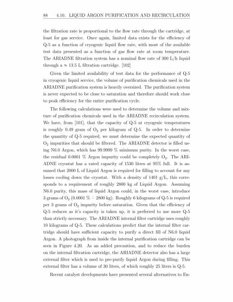
88 4.10. LIQUID ARGON PURIFICATION AND RECIRCULATION
the filtration rate is proportional to the flow rate through the cartridge, at
least for gas service. Once again, limited data exists for the efficiency of
Q-5 as a function of cryogenic liquid flow rate, with most of the available
test data presented as a function of gas flow rate at room temperature.
The ARIADNE filtration system has a nominal flow rate of 300 L/h liquid
through a 13.5 L filtration cartridge. [102]
Given the limited availability of test data for the performance of Q-5
in cryogenic liquid service, the volume of purification chemicals used in the
ARIADNE purification system is heavily oversized. The purification system
is never expected to be close to saturation and therefore should work close
to peak efficiency for the entire purification cycle.
The following calculations were used to determine the volume and mix-
ture of purification chemicals used in the ARIADNE recirculation system.
We have, from [101], that the capacity of Q-5 at cryogenic temperatures
is roughly 0.49 gram of O2 per kilogram of Q-5. In order to determine
the quantity of Q-5 required, we must determine the expected quantity of
O2 impurities that should be filtered. The ARIADNE detector is filled us-
ing N6.0 Argon, which has 99.9999 % minimum purity. In the worst case,
the residual 0.0001 % Argon impurity could be completely O2. The ARI-
ADNE cryostat has a rated capacity of 1530 litres at 95% full. It is as-
sumed that 2000 L of Liquid Argon is required for filling to account for any
losses cooling down the cryostat. With a density of 1401 g/L, this corre-
sponds to a requirement of roughly 2800 kg of Liquid Argon. Assuming
N6.0 purity, this mass of liquid Argon could, in the worst case, introduce
3 grams of O2 (0.0001 % 2800 kg). Roughly 6 kilograms of Q-5 is required
per 3 grams of O2 impurity before saturation. Given that the efficiency of
Q-5 reduces as it’s capacity is taken up, it is preferred to use more Q-5
than strictly necessary. The ARIADNE internal filter cartridge uses roughly
10 kilograms of Q-5. These calculations predict that the internal filter car-
tridge should have sufficient capacity to purify a direct fill of N6.0 liquid
Argon. A photograph from inside the internal purification cartridge can be
seen in Figure 4.20. As an added precaution, and to reduce the burden
on the internal filtration cartridge, the ARIADNE detector also has a large
external filter which is used to pre-purify liquid Argon during filling. This
external filter has a volume of 30 liters, of which roughly 25 liters is Q-5.
Recent catalyst developments have presented several alternatives to En-
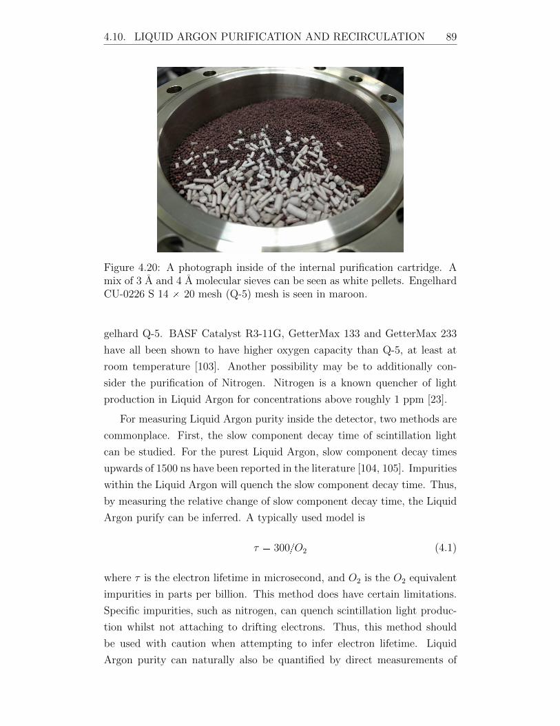
4.10. LIQUID ARGON PURIFICATION AND RECIRCULATION 89
Figure 4.20: A photograph inside of the internal purification cartridge. Amix of 3 A and 4 A molecular sieves can be seen as white pellets. EngelhardCU-0226 S 14 20 mesh (Q-5) mesh is seen in maroon.
gelhard Q-5. BASF Catalyst R3-11G, GetterMax 133 and GetterMax 233
have all been shown to have higher oxygen capacity than Q-5, at least at
room temperature [103]. Another possibility may be to additionally con-
sider the purification of Nitrogen. Nitrogen is a known quencher of light
production in Liquid Argon for concentrations above roughly 1 ppm [23].
For measuring Liquid Argon purity inside the detector, two methods are
commonplace. First, the slow component decay time of scintillation light
can be studied. For the purest Liquid Argon, slow component decay times
upwards of 1500 ns have been reported in the literature [104, 105]. Impurities
within the Liquid Argon will quench the slow component decay time. Thus,
by measuring the relative change of slow component decay time, the Liquid
Argon purify can be inferred. A typically used model is
τ 300O2 (4.1)
where τ is the electron lifetime in microsecond, and O2 is the O2 equivalent
impurities in parts per billion. This method does have certain limitations.
Specific impurities, such as nitrogen, can quench scintillation light produc-
tion whilst not attaching to drifting electrons. Thus, this method should
be used with caution when attempting to infer electron lifetime. Liquid
Argon purity can naturally also be quantified by direct measurements of
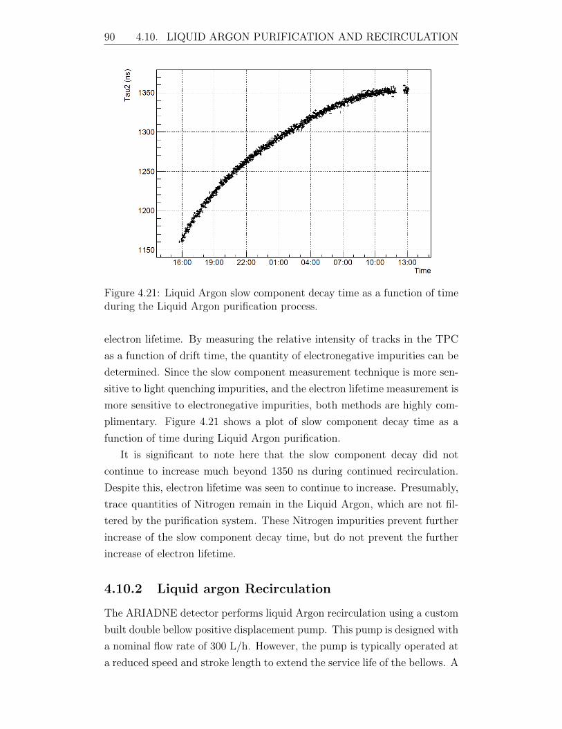
90 4.10. LIQUID ARGON PURIFICATION AND RECIRCULATION
Figure 4.21: Liquid Argon slow component decay time as a function of timeduring the Liquid Argon purification process.
electron lifetime. By measuring the relative intensity of tracks in the TPC
as a function of drift time, the quantity of electronegative impurities can be
determined. Since the slow component measurement technique is more sen-
sitive to light quenching impurities, and the electron lifetime measurement is
more sensitive to electronegative impurities, both methods are highly com-
plimentary. Figure 4.21 shows a plot of slow component decay time as a
function of time during Liquid Argon purification.
It is significant to note here that the slow component decay did not
continue to increase much beyond 1350 ns during continued recirculation.
Despite this, electron lifetime was seen to continue to increase. Presumably,
trace quantities of Nitrogen remain in the Liquid Argon, which are not fil-
tered by the purification system. These Nitrogen impurities prevent further
increase of the slow component decay time, but do not prevent the further
increase of electron lifetime.
4.10.2 Liquid argon Recirculation
The ARIADNE detector performs liquid Argon recirculation using a custom
built double bellow positive displacement pump. This pump is designed with
a nominal flow rate of 300 L/h. However, the pump is typically operated at
a reduced speed and stroke length to extend the service life of the bellows. A

4.10. LIQUID ARGON PURIFICATION AND RECIRCULATION 91
diagram showing the general operating principle of the re-circulation system
is shown in Figure 4.22.
The air side bellow of the ARIADNE pump system is driven by a custom
designed linear motion assembly. The assembly is designed with minimal
footprint on the ARIADNE flange so as to not interfere with neighboring
feedthroughs and ports. A CAD drawing of the pump drive system is shown
in Figure 4.23.
The system was designed to be easy to operate while retaining flexibility.
It should be possible to quickly change certain pumping parameters such as
stroke length and pumping speed without an extensive understanding of the
system. The mechanical design of the system can be split up into several
components. First is the supporting frame. This frame is formed from three
standard linear shafts from Misumi. These shafts provide generous mechani-
cal strength to the assembly but also double up as the linear motion solution.
Three IGUS maintenance-free linear bearings run along the outer diameter
of these shafts. The combined used of these shafts for structural as well as
linear motion helps maintain the small footprint of the assembly. The three
linear bushings are bolted to the plate which will perform the reciprocating
motion. This plate is connected to the top of the bellow using three stainless
steel shafts. By moving this plate, the bellow can be compressed or extended
and thus the pump can be operated. The motion of this plate is driven by
a 16 mm diameter, 50 mm pitch ballscrew. The high pitch of this ballscrew
enables a fast pumping speed. The axial force generated by this ballscrew
during pumping can be significant. These axial loads are far in excess of the
loads that the bearings in the driving motor are capable of handling directly.
Most motors are generally only rated for very modest axial loads so it is a
good practice to handle these forces before the motor. The ballscrew used
in the assembly has a stepped and threaded end. The end of the ballscrew
is retained into a fixed end support in a secondary fixed plate, above the
reciprocating plate. This fixed plate takes up all of the axial load of the
ballscrew so that the motor bearings are protected.
A fixed mounting bracket is provided at the top of the assembly for
mounting a NEMA34 frame size motor. Originally a stepper mounted was
mounted here but this motor was later replaced with a Clearpath integrated
servo motor. The motor shaft is coupled to the ballscrew using a stainless
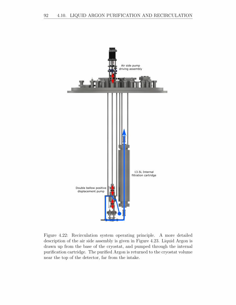
92 4.10. LIQUID ARGON PURIFICATION AND RECIRCULATION
13.5L Internalfiltration cartridge
Double bellow positivedisplacement pump
Air side pumpdriving assembly
Figure 4.22: Recirculation system operating principle. A more detaileddescription of the air side assembly is given in Figure 4.23. Liquid Argon isdrawn up from the base of the cryostat, and pumped through the internalpurification cartridge. The purified Argon is returned to the cryostat volumenear the top of the detector, far from the intake.
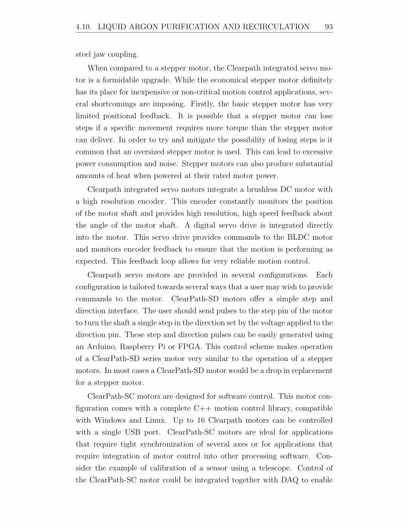
4.10. LIQUID ARGON PURIFICATION AND RECIRCULATION 93
steel jaw coupling.
When compared to a stepper motor, the Clearpath integrated servo mo-
tor is a formidable upgrade. While the economical stepper motor definitely
has its place for inexpensive or non-critical motion control applications, sev-
eral shortcomings are imposing. Firstly, the basic stepper motor has very
limited positional feedback. It is possible that a stepper motor can lose
steps if a specific movement requires more torque than the stepper motor
can deliver. In order to try and mitigate the possibility of losing steps is it
common that an oversized stepper motor is used. This can lead to excessive
power consumption and noise. Stepper motors can also produce substantial
amounts of heat when powered at their rated motor power.
Clearpath integrated servo motors integrate a brushless DC motor with
a high resolution encoder. This encoder constantly monitors the position
of the motor shaft and provides high resolution, high speed feedback about
the angle of the motor shaft. A digital servo drive is integrated directly
into the motor. This servo drive provides commands to the BLDC motor
and monitors encoder feedback to ensure that the motion is performing as
expected. This feedback loop allows for very reliable motion control.
Clearpath servo motors are provided in several configurations. Each
configuration is tailored towards several ways that a user may wish to provide
commands to the motor. ClearPath-SD motors offer a simple step and
direction interface. The user should send pulses to the step pin of the motor
to turn the shaft a single step in the direction set by the voltage applied to the
direction pin. These step and direction pulses can be easily generated using
an Arduino, Raspberry Pi or FPGA. This control scheme makes operation
of a ClearPath-SD series motor very similar to the operation of a stepper
motors. In most cases a ClearPath-SD motor would be a drop in replacement
for a stepper motor.
ClearPath-SC motors are designed for software control. This motor con-
figuration comes with a complete C++ motion control library, compatible
with Windows and Linux. Up to 16 Clearpath motors can be controlled
with a single USB port. ClearPath-SC motors are ideal for applications
that require tight synchronization of several axes or for applications that
require integration of motor control into other processing software. Con-
sider the example of calibration of a sensor using a telescope. Control of
the ClearPath-SC motor could be integrated together with DAQ to enable
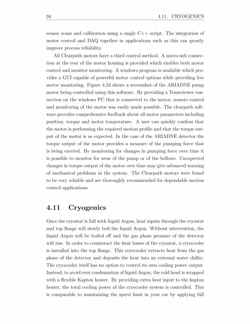
94 4.11. CRYOGENICS
sensor scans and calibration using a single C++ script. The integration of
motor control and DAQ together in applications such as this can greatly
improve process reliability.
All Clearpath motors have a third control method. A micro-usb connec-
tion at the rear of the motor housing is provided which enables both motor
control and monitor monitoring. A windows program is available which pro-
vides a GUI capable of powerful motor control options while providing live
motor monitoring. Figure 4.24 shows a screenshot of the ARIADNE pump
motor being controlled using this software. By providing a Teamviewer con-
nection on the windows PC that is connected to the motor, remote control
and monitoring of the motor was easily made possible. The clearpath soft-
ware provides comprehensive feedback about all motor parameters including
position, torque and motor temperature. A user can quickly confirm that
the motor is performing the required motion profile and that the torque out-
put of the motor is as expected. In the case of the ARIADNE detector the
torque output of the motor provides a measure of the pumping force that
is being exerted. By monitoring for changes in pumping force over time it
is possible to monitor for wear of the pump or of the bellows. Unexpected
changes in torque output of the motor over time may give advanced warning
of mechanical problems in the system. The Clearpath motors were found
to be very reliable and are thoroughly recommended for dependable motion
control applications.
4.11 Cryogenics
Once the cryostat is full with liquid Argon, heat inputs through the cryostat
and top flange will slowly boil the liquid Argon. Without intervention, the
liquid Argon will be boiled off and the gas phase pressure of the detector
will rise. In order to counteract the heat losses of the cryostat, a cryocooler
is installed into the top flange. This cryocooler extracts heat from the gas
phase of the detector and deposits the heat into an external water chiller.
The cryocooler itself has no option to control its own cooling power output.
Instead, to avoid over condensation of liquid Argon, the cold head is wrapped
with a flexible Kapton heater. By providing extra heat input to the kapton
heater, the total cooling power of the cryocooler system is controlled. This
is comparable to maintaining the speed limit in your car by applying full
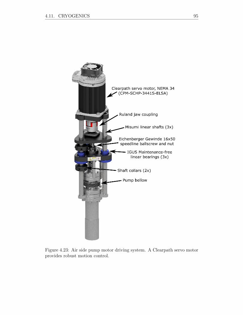
4.11. CRYOGENICS 95
Figure 4.23: Air side pump motor driving system. A Clearpath servo motorprovides robust motion control.
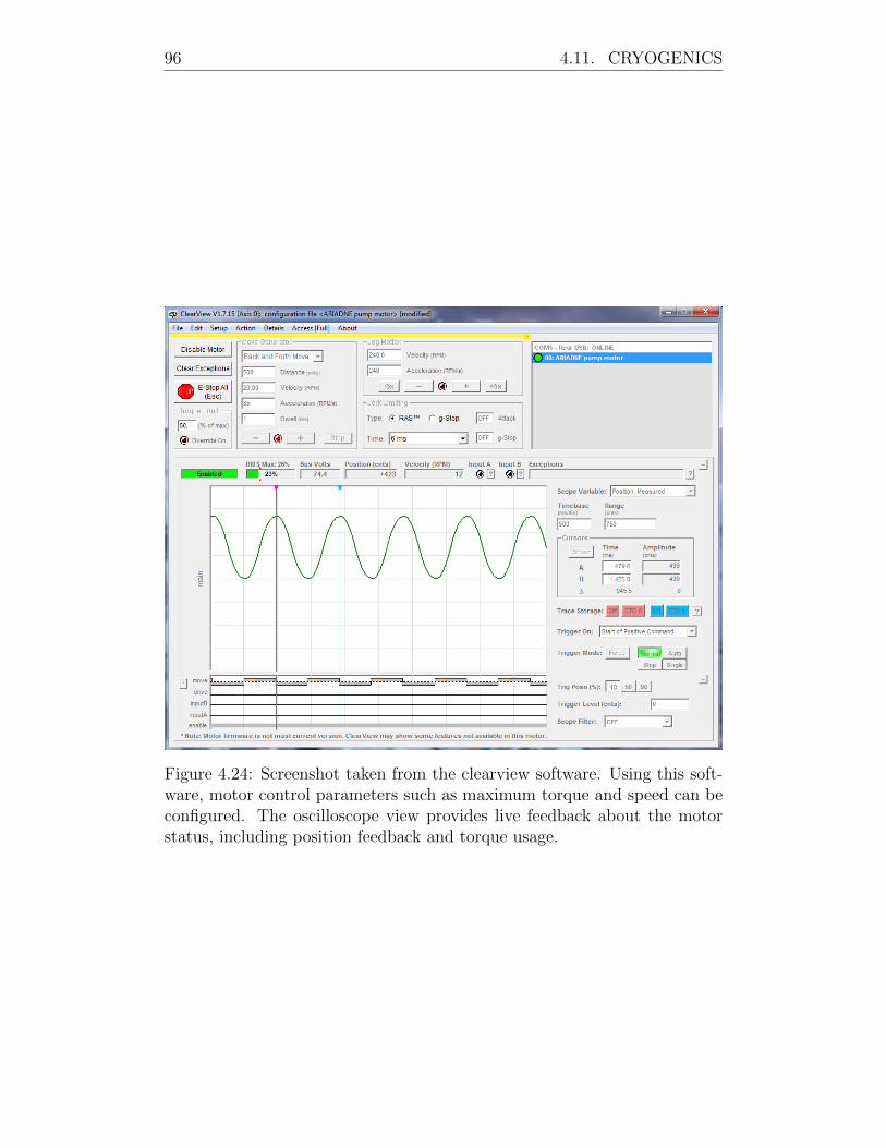
96 4.11. CRYOGENICS
Figure 4.24: Screenshot taken from the clearview software. Using this soft-ware, motor control parameters such as maximum torque and speed can beconfigured. The oscilloscope view provides live feedback about the motorstatus, including position feedback and torque usage.
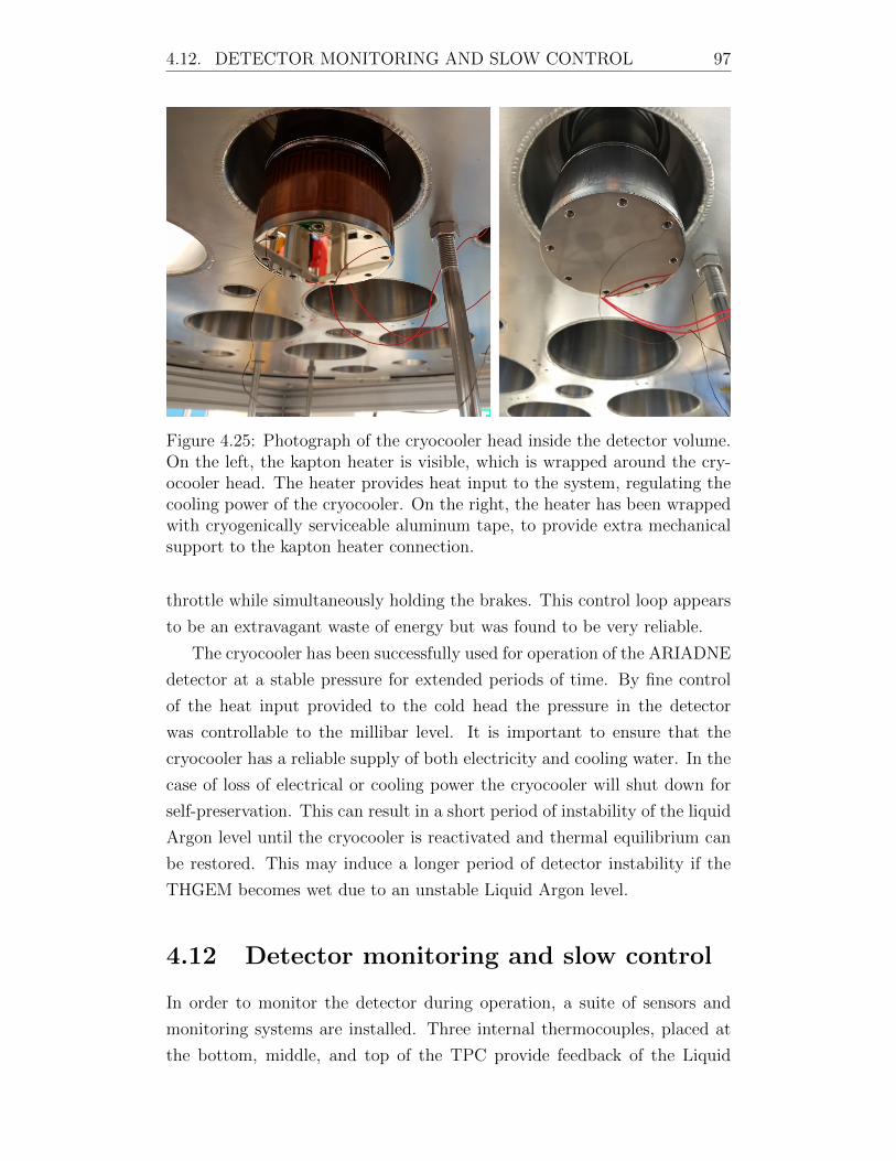
4.12. DETECTOR MONITORING AND SLOW CONTROL 97
Figure 4.25: Photograph of the cryocooler head inside the detector volume.On the left, the kapton heater is visible, which is wrapped around the cry-ocooler head. The heater provides heat input to the system, regulating thecooling power of the cryocooler. On the right, the heater has been wrappedwith cryogenically serviceable aluminum tape, to provide extra mechanicalsupport to the kapton heater connection.
throttle while simultaneously holding the brakes. This control loop appears
to be an extravagant waste of energy but was found to be very reliable.
The cryocooler has been successfully used for operation of the ARIADNE
detector at a stable pressure for extended periods of time. By fine control
of the heat input provided to the cold head the pressure in the detector
was controllable to the millibar level. It is important to ensure that the
cryocooler has a reliable supply of both electricity and cooling water. In the
case of loss of electrical or cooling power the cryocooler will shut down for
self-preservation. This can result in a short period of instability of the liquid
Argon level until the cryocooler is reactivated and thermal equilibrium can
be restored. This may induce a longer period of detector instability if the
THGEM becomes wet due to an unstable Liquid Argon level.
4.12 Detector monitoring and slow control
In order to monitor the detector during operation, a suite of sensors and
monitoring systems are installed. Three internal thermocouples, placed at
the bottom, middle, and top of the TPC provide feedback of the Liquid
98 4.12. DETECTOR MONITORING AND SLOW CONTROL
Argon level during filling and emptying. In principle these thermocouples
could be used to monitor temperature gradients in the TPC but since they
were not calibrated this study has not yet been performed. An additional
internal thermocouple is mounted to the underside of the top flange using
kapton tape with a matching thermocouple mounted externally on the top of
the flange. This thermocouple pair is mainly used to estimate the heat losses
that should be present through the flange. A final external thermocouple is
attached arbitrarily to the cryostat outer wall. Trends in this thermocouples
temperature can be used to infer the condition of the vacuum jacket of the
cryostat.
Two internal webcams provide feedback on the Liquid Argon level close
to the THGEM as well as provide a view of the internal recirculation system.
The first webcam is used to ensure that the Liquid level is roughly parallel to
the THGEM. The second webcam provides video feedback of Liquid Argon
recirculation which is used to confirm that the Liquid Argon pump is func-
tioning well. These internal webcams require light to operate so a selection
of individually controllable LEDs are installed around the top of the TPC.
These LEDs provide both blue and red illumination to all key parts of the
detector which can be seen by the webcams.
Pressure monitoring is performed using two pressure sensors. One pres-
sure sensor is better suited to monitor overpressure, whilst the other is only
used when evacuating the cryostat, and provides accurate pressure readings
down to 1E-9 mbar.
Chapter 5
The ARIADNE detector
exposed to the CERN T9
beamline
The performance of the ARIADNE detector using EMCCD cameras was
tested at the CERN T9 beamline in March/April 2018. The T9 beamline is
a mixed charge particle testbeam, providing a mixture of electrons, muons,
pions, kaons and protons in a momentum range between 0.5 - 8 GeV/c.
Before the experiment was deployed to the beamline, Geant4 beamline sim-
ulations were performed. These are discussed in Section 5.1. A gallery of
events and discussion of detector operation at the beamline is presented in
Section 5.2.
5.1 Beamline simulation
The goal of the T9 beamline simulation was to provide a better understand-
ing of the particle flux that could be expected at the reference focus of the
beamline. Available documentation for the T9 beamline [106] only provides
composition of the beam at the production target, not at the reference focus.
Certain, short lived, particles such as as pions, may decay in the beamline
and not reach the experimental area. The beamline simulation allowed us
to quantify these effects, to make more informed decisions about which mo-
mentum range should be scanned during data taking. Figure 5.1 shows a
photograph of a section of the beamline, immediately upstream of the exper-
imental area. In this photograph we can identify two quadrupole magnets
99
100 5.1. BEAMLINE SIMULATION
in blue, a dipole magnet in green, and a short gap in the beamline which
can be used for installing time of flight systems. Two large concrete/iron
shielding elements are visible in red, both of which are found after dipole
magnets. These shielded elements absorb particles which are not successfully
transported by the dipole magnets, shielding the experimental area.
The beamline simulation was constructed completely from Geant4 prim-
itives. More complete packages for beamline simulation do exist, such as
G4Beamline, but these packages are more tailored towards beamline design,
rather than using the beamline to produce a particle sample to be delivered
to a simulated detector. The geometry of the beamline was constructed
using publicly available CAD models of the beamline. Figure 5.2 shows a
schematic of the T9 beamline, and two screenshots of the simulated geome-
try. In the simulated geometry we can identify the quadrupole magnets as
blue and the dipole magnets as green. The concrete shielding of the beam-
line is visible in white. The ARIADNE detector is seen on the far right,
sitting at the reference focus of the beamline.
The magnet parameters of the beamline were initially approximately
using publicly available values of the current delivered to each magnet. These
values were then fine tuned until the transport properties of the beamline
were in rough agreement with the simulations that were performed by CERN
during the beam commissioning [107]. Figure 5.3 shows the simulated beam
profiles as a function of position along the beamline, for both horizontal and
vertical planes.
The simulations provided guidance for detector placement in the experi-
mental area. From the simulations, it was found that the detector need not
be positioned extremely precisely in the experimental area, since the beam is
mostly coherent over a few meters at the reference focus. For computational
reasons, the initial products of the beamline at the north multitarget were
assumed, distributed according to simulations produced by CERN. This as-
sumption however misses one detail about beamline operation. During the
interaction of the PS beam with the north multitarget, a large quantity
of muons, distributed over a wide momentum range, are produced. These
muons easily pass through the beamline shielding and produce a background
of events in the detector. These muons are often called beam halo muons.
Had the interaction of the PS beam on the north multitarget been simu-
lated, the beamline simulation may have provided information about the
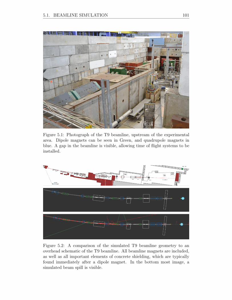
5.1. BEAMLINE SIMULATION 101
Figure 5.1: Photograph of the T9 beamline, upstream of the experimentalarea. Dipole magnets can be seen in Green, and quadrupole magnets inblue. A gap in the beamline is visible, allowing time of flight systems to beinstalled.
Figure 5.2: A comparison of the simulated T9 beamline geometry to anoverhead schematic of the T9 beamline. All beamline magnets are included,as well as all important elements of concrete shielding, which are typicallyfound immediately after a dipole magnet. In the bottom most image, asimulated beam spill is visible.
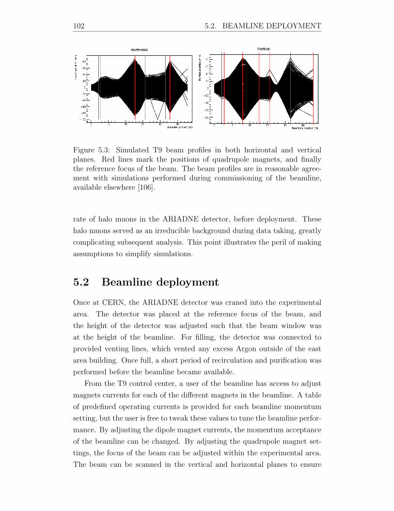
102 5.2. BEAMLINE DEPLOYMENT
Figure 5.3: Simulated T9 beam profiles in both horizontal and verticalplanes. Red lines mark the positions of quadrupole magnets, and finallythe reference focus of the beam. The beam profiles are in reasonable agree-ment with simulations performed during commissioning of the beamline,available elsewhere [106].
rate of halo muons in the ARIADNE detector, before deployment. These
halo muons served as an irreducible background during data taking, greatly
complicating subsequent analysis. This point illustrates the peril of making
assumptions to simplify simulations.
5.2 Beamline deployment
Once at CERN, the ARIADNE detector was craned into the experimental
area. The detector was placed at the reference focus of the beam, and
the height of the detector was adjusted such that the beam window was
at the height of the beamline. For filling, the detector was connected to
provided venting lines, which vented any excess Argon outside of the east
area building. Once full, a short period of recirculation and purification was
performed before the beamline became available.
From the T9 control center, a user of the beamline has access to adjust
magnets currents for each of the different magnets in the beamline. A table
of predefined operating currents is provided for each beamline momentum
setting, but the user is free to tweak these values to tune the beamline perfor-
mance. By adjusting the dipole magnet currents, the momentum acceptance
of the beamline can be changed. By adjusting the quadrupole magnet set-
tings, the focus of the beam can be adjusted within the experimental area.
The beam can be scanned in the vertical and horizontal planes to ensure
5.2. BEAMLINE DEPLOYMENT 103
good alignment with the beam window.
The user also has access to collimator controls, which allows for fine
control over the beam flux. The collimators are two sets of movable jaws, in
two planes perpendicular to the beam axis. Closing the collimators causes
the jaws to impinge into the beam profile, reducing the rate of particles
reaching the experimental area. Generally, the collimators were tuned to
provide approximately 20 particles per spill, to minimise pileup. Each spill
of the beamline has a duration of 350 ms, during which particles are provided
uniformly, within a time tolerance of nanoseconds. The EMCCD cameras
were found to operate best at a rate close to 50 Hz, and an exposure time
of 400 microseconds. 20 particles provided during a 350 millisecond beam
window, translates to one particle roughly every 17.5 milliseconds. This
rate is in line with the maximum 50 Hz readout rate of the cameras, and the
chance of pileup of beamline particles was expected to be minimal. As was
earlier discussed, each beamline spill also provided an irreducible background
of halo muons. Thus, each event window generally contained one or fewer
beamline particles, plus this halo muon background.
Due to ongoing building works in the experimental area, a scaffolding
was constructed around and above the detector, providing protection from
works overhead. Figure 5.4 shows several photographs of the ARIADNE
experiment at the T9 beamline.
Typically, the ARIADNE detector was operated with a drift field of
960 V/cm. Given the strict timelines of beamline operation, limited time
for purification was available. The larger drift field helped to compensate
for the less than nominal electron lifetime. An electrical fault with the
THGEM feedthrough meant that the maximum bias that could be applied
to the THGEM was 2.7 kV. Later testing in Liverpool found that during
manufacture, the ceramic insulation of the feedthrough had been damaged
during the welding process. This damage reduced the insulating capability
of the feedthrough, limiting the maximum bias that was possible. At the
lower THGEM bias of 2.7 kV, light production from the THGEM is quite
heavily suppressed. Figure 5.5 shows a calibration performed of the THGEM
at Liverpool, with a full functional feedthrough. From the Figure, a clear
suppression of light production is seen at 2.7 kV. If operated at the nominal
bias of 3.2 kV, at least double the light output could be expected.
Despite this large reduction in light production, data taking was still
104 5.2. BEAMLINE DEPLOYMENT
possible with a reasonable level of signal to noise. Over the 18 days of beam
time, a total of 800,000 events were collected, mostly below 2 GeV/c. Figure
5.7 shows two selected events from the data taken at T9. Analysis is ongoing
with data taken from the beamline.
As well as beamline events, several interesting cosmic events were also
seen during operation at CERN. Figure 5.8 shows an event display of a cos-
mic air shower. After inspecting the data that was taken, it was clear that
excellent px, yq resolution was possible. Yet, operation at the T9 beamline
highlighted a key challenge of optical readout using EMCCDs, namely z
dimension reconstruction. The general principle of 3D reconstruction was
that the EMCCD readout channel should be combined with a faster read-
out channel, such as a PMT, to recover z position information about the
track. By performing pulse shape analysis, it is possible to determine both
the depth and extent of an event in the z-axis. The topmost part of the
track can be identified by measuring the time delay between the S1 and S2
signals on the PMT. The total extent of the track in z can be determined
by measuring the total time duration of the S2 pulse. The general principle
of this reconstruction method is shown in Figure 5.6. The S2 signal is seen
to be distinct from the S1 signal, which allows the depth of the event in the
TPC to be determined. The duration and intensity of the S2 profile allows
information about the event in the z dimension to be inferred.
Although this method had proven to be quite robust for simple through-
going cosmic muons, the beamline environment was much more challenging.
Considering an isolated electromagnetic shower; the task of assigning seg-
ments of a PMT S2 pulse to individual branches of the shower is mostly
intractable. This challenge was compounded by the highly active environ-
ment of the beamline. The halo muons from the PS beamline accompanied
each beam spill, essentially guaranteeing pileup within any event window.
Figure 5.9 shows an event display containing the typical level of halo muon
contamination. Following return from the beamline, substantial R&D effort
began to tackle this limitation. This R&D effort culminated in the devel-
opment of a novel optical readout technology, which enables full px, y, zqreconstruction using a camera. This development is presented in Chapter 6.
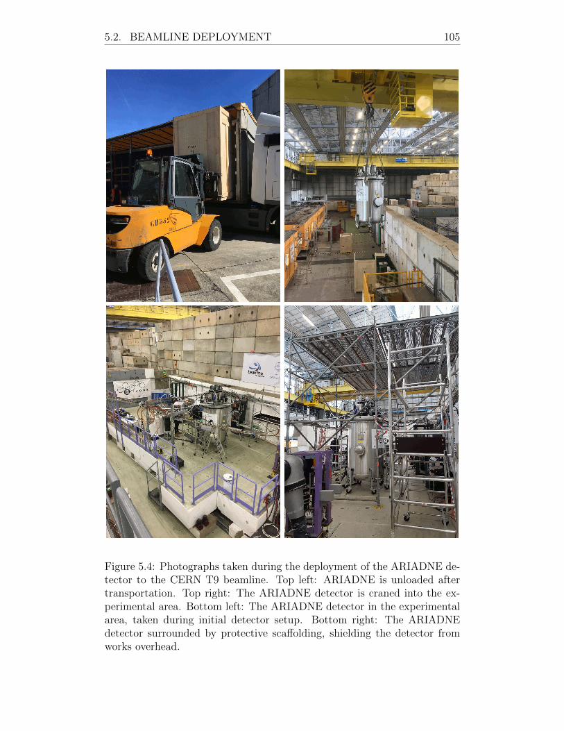
5.2. BEAMLINE DEPLOYMENT 105
Figure 5.4: Photographs taken during the deployment of the ARIADNE de-tector to the CERN T9 beamline. Top left: ARIADNE is unloaded aftertransportation. Top right: The ARIADNE detector is craned into the ex-perimental area. Bottom left: The ARIADNE detector in the experimentalarea, taken during initial detector setup. Bottom right: The ARIADNEdetector surrounded by protective scaffolding, shielding the detector fromworks overhead.
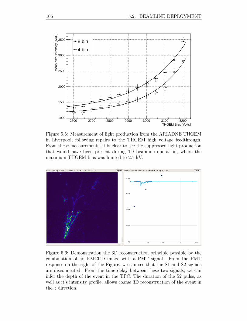
106 5.2. BEAMLINE DEPLOYMENT
2600 2700 2800 2900 3000 3100 3200THGEM Bias [Volts]
1000
1500
2000
2500
3000
3500
Mea
n pi
xel i
nten
sity
[AD
U]
8 bin
4 bin
Figure 5.5: Measurement of light production from the ARIADNE THGEMin Liverpool, following repairs to the THGEM high voltage feedthrough.From these measurements, it is clear to see the suppressed light productionthat would have been present during T9 beamline operation, where themaximum THGEM bias was limited to 2.7 kV.
Figure 5.6: Demonstration the 3D reconstruction principle possible by thecombination of an EMCCD image with a PMT signal. From the PMTresponse on the right of the Figure, we can see that the S1 and S2 signalsare disconnected. From the time delay between these two signals, we caninfer the depth of the event in the TPC. The duration of the S2 pulse, aswell as it’s intensity profile, allows coarse 3D reconstruction of the event inthe z direction.
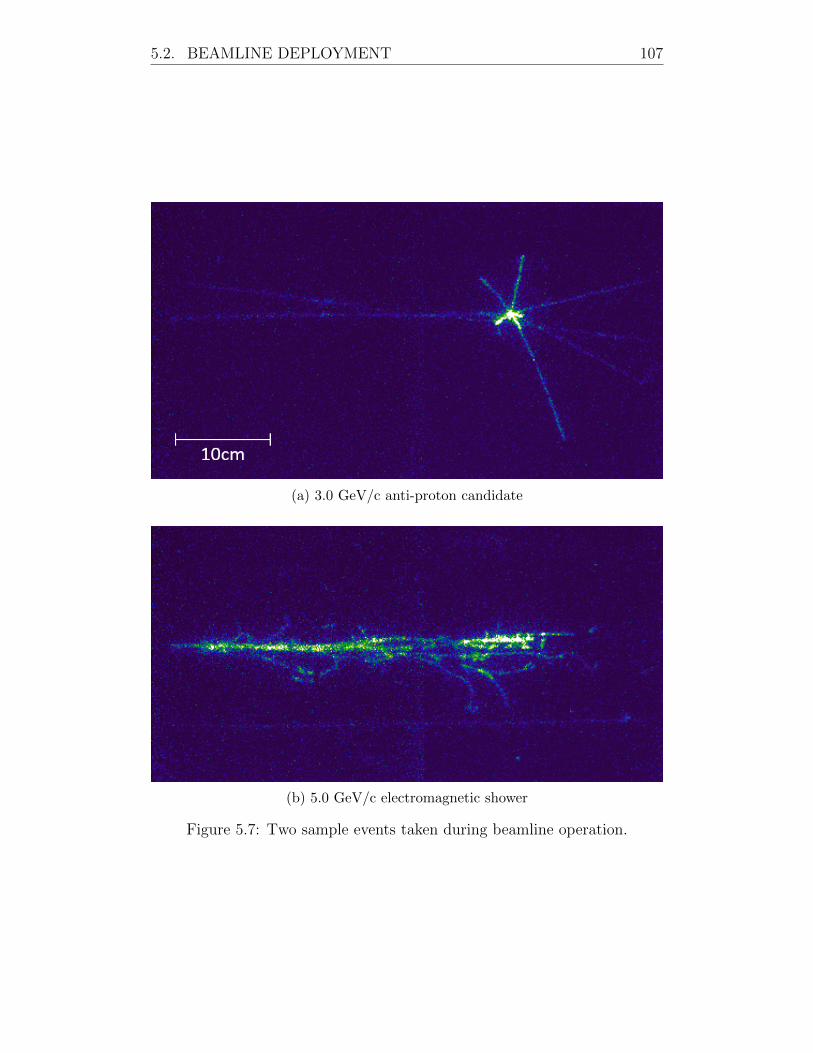
5.2. BEAMLINE DEPLOYMENT 107
(a) 3.0 GeV/c anti-proton candidate
(b) 5.0 GeV/c electromagnetic shower
Figure 5.7: Two sample events taken during beamline operation.
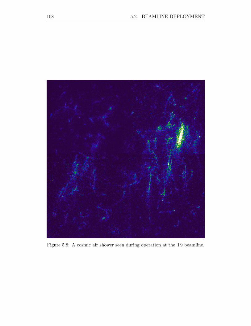
108 5.2. BEAMLINE DEPLOYMENT
Figure 5.8: A cosmic air shower seen during operation at the T9 beamline.
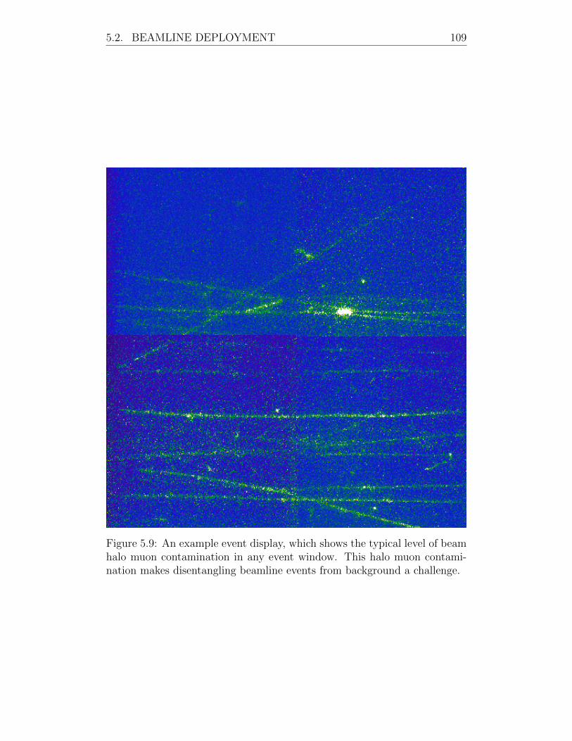
5.2. BEAMLINE DEPLOYMENT 109
Figure 5.9: An example event display, which shows the typical level of beamhalo muon contamination in any event window. This halo muon contami-nation makes disentangling beamline events from background a challenge.
Chapter 6
Development of Timepix 3
based camera readout
Results from the T9 beamlined showed that excellent px, yq resolution was
possible with optical readout. The z dimension however, remained a chal-
lenge. Moreover, the frame based readout can also be limiting. EMCCD
cameras operate by integrating light over a predefined exposure time. Given
the drift velocity of electrons in LAr is 1.6mm/µs at 0.5 kV/cm, an expo-
sure time of less than 500 ns would be required for z position resolution on
the millimeter scale. This infers a frame rate of 2 MHz, unattainable using
today’s commercial EMCCD or CMOS camera technologies. Moreover, even
if this frame rate was possible, the ensuing data rate would be practically
unmanageable. Early on during R&D efforts, it became clear that high reso-
lution z position tracking would require a new approach. Such an approach
was developed using a camera based on the Timepix 3 (TPX3) ASIC. The
crucial benefit of this ASIC is the escape from frame-based readout.
6.1 The Timepix3 ASIC
Timepix 3 (TPX3) [108] is a general purpose ASIC, designed to provide si-
multaneous intensity and timing information for detected signals. Each pixel
of TPX3 contains an individually customisable pre-amplifier and digitiser.
The general operating principle of the TPX3 ASIC is described as follows
1. Signal arrives at a pixel of TPX3
2. The pre-amplifer in the pixel integrates the signal that is received. If
110
6.1. THE TIMEPIX3 ASIC 111
this charge signal goes above a predefined pixel threshold, then the
readout process begins. If the signal does not exceed the pixel thresh-
old then the pixel is not readout (it is zero-supressed).
3. The time at which the pre-amplifier signal crosses the pixel threshold is
known as the Time of Arrival (ToA). This value has 1.6 ns resolution,
limited by the 640 MHz fast time of arrival clock within the TPX3
ASIC.
4. The pre-amplifer signal begins to decay. The time duration between
the pre-amplifier signal rising over the pixel threshold and decaying
below the pixel threshold is known as Time over Threshold (ToT).
This value is proportional to the intensity of the signal and is stored
with 10-bit resolution.
5. A packet of data containing ToA, ToT and pixel address information is
created and readout from the ASIC. The pixel address is a 16-bit value
which encodes the pixel’s px, yq location on the ASIC. This readout
step incurs a 475 ns pixel dead time.
6. After the 475 ns dead time, the pixel is ready for the next event.
The TPX3 ASIC is a general purpose readout chip, designed to be suit-
able for a wide variety of applications. Thus, a wide selection of parameters
are available through which the response of the ASIC can be customised.
For best performance, these parameters should be reasonably well tuned to
the specific application. The effect of some of these parameters is illustrated
on Figure 6.1. One important settings is the pixel Krummenacher current.
This current dictates the decay time of the pre-amplifier. A high current
allows a fast pre-amplifier decay and visa versa. If the pre-amplifier decay
time is too short, the full 10-bit ToT range may not be used. Conversely, if
the decay time is too long, hits may saturate the 10-bit range and calorimet-
ric information may be lost. During operation, this value was tuned to try
and best use the 10-bit ToT range. Other parameters, such as rise time of
the pre-amplifier, can also be customised. Ideally, the rise time should be as
fast as possible. If the rise time is slow, the time at which the pre-amplifier
signal crosses the pixel threshold can be different from the time at which
the signal hit the pixel. This effect is known as time walk. The drawback
of a fast pre-amplifier rise time is increased heat output and power draw
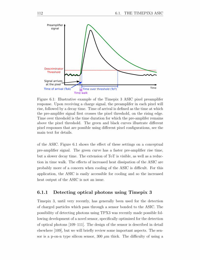
112 6.1. THE TIMEPIX3 ASIC
Preamplifiersignal
DescriminatorThreshold
Signal arrivesat the pixel
Time over threshold (ToT)Time of arrival (ToA)
Time walk
Time
Figure 6.1: Illustrative example of the Timepix 3 ASIC pixel preampliferresponse. Upon receiving a charge signal, the preamplifer in each pixel willrise, followed by a decay time. Time of arrival is defined as the time at whichthe pre-amplifer signal first crosses the pixel threshold, on the rising edge.Time over threshold is the time duration for which the pre-amplifer remainsabove the pixel threshold. The green and black curves illustrate differentpixel responses that are possible using different pixel configurations, see themain text for details.
of the ASIC. Figure 6.1 shows the effect of these settings on a conceptual
pre-amplifier signal. The green curve has a faster pre-amplifier rise time,
but a slower decay time. The extension of ToT is visible, as well as a reduc-
tion in time walk. The effects of increased heat dissipation of the ASIC are
probably more of a concern when cooling of the ASIC is difficult. For this
application, the ASIC is easily accessible for cooling and so the increased
heat output of the ASIC is not an issue.
6.1.1 Detecting optical photons using Timepix 3
Timepix 3, until very recently, has generally been used for the detection
of charged particles which pass through a sensor bonded to the ASIC. The
possibility of detecting photons using TPX3 was recently made possible fol-
lowing development of a novel sensor, specifically optimised for the detection
of optical photons [109–111]. The design of the sensor is described in detail
elsewhere [109], but we will briefly review some important aspects. The sen-
sor is a p-on-n type silicon sensor, 300 µm thick. The difficulty of using a
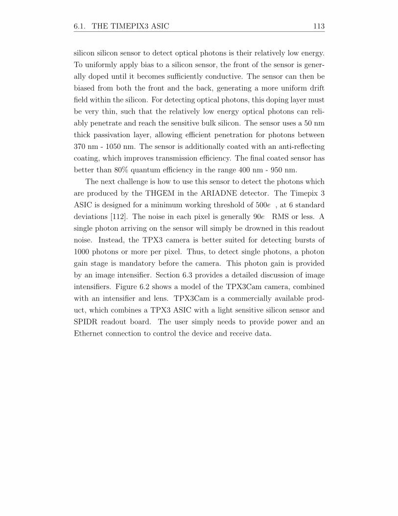
6.1. THE TIMEPIX3 ASIC 113
silicon silicon sensor to detect optical photons is their relatively low energy.
To uniformly apply bias to a silicon sensor, the front of the sensor is gener-
ally doped until it becomes sufficiently conductive. The sensor can then be
biased from both the front and the back, generating a more uniform drift
field within the silicon. For detecting optical photons, this doping layer must
be very thin, such that the relatively low energy optical photons can reli-
ably penetrate and reach the sensitive bulk silicon. The sensor uses a 50 nm
thick passivation layer, allowing efficient penetration for photons between
370 nm - 1050 nm. The sensor is additionally coated with an anti-reflecting
coating, which improves transmission efficiency. The final coated sensor has
better than 80% quantum efficiency in the range 400 nm - 950 nm.
The next challenge is how to use this sensor to detect the photons which
are produced by the THGEM in the ARIADNE detector. The Timepix 3
ASIC is designed for a minimum working threshold of 500e, at 6 standard
deviations [112]. The noise in each pixel is generally 90e RMS or less. A
single photon arriving on the sensor will simply be drowned in this readout
noise. Instead, the TPX3 camera is better suited for detecting bursts of
1000 photons or more per pixel. Thus, to detect single photons, a photon
gain stage is mandatory before the camera. This photon gain is provided
by an image intensifier. Section 6.3 provides a detailed discussion of image
intensifiers. Figure 6.2 shows a model of the TPX3Cam camera, combined
with an intensifier and lens. TPX3Cam is a commercially available prod-
uct, which combines a TPX3 ASIC with a light sensitive silicon sensor and
SPIDR readout board. The user simply needs to provide power and an
Ethernet connection to control the device and receive data.
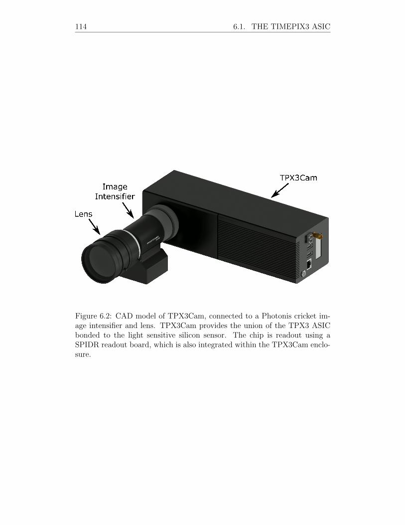
114 6.1. THE TIMEPIX3 ASIC
Figure 6.2: CAD model of TPX3Cam, connected to a Photonis cricket im-age intensifier and lens. TPX3Cam provides the union of the TPX3 ASICbonded to the light sensitive silicon sensor. The chip is readout using aSPIDR readout board, which is also integrated within the TPX3Cam enclo-sure.
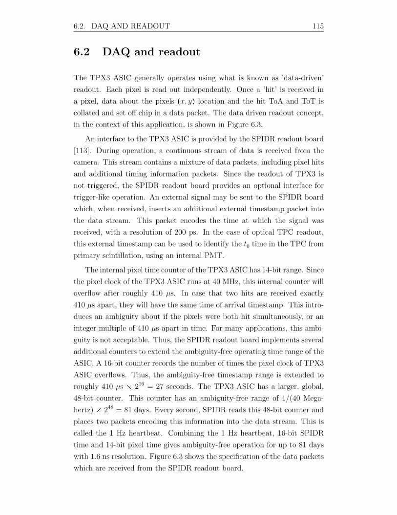
6.2. DAQ AND READOUT 115
6.2 DAQ and readout
The TPX3 ASIC generally operates using what is known as ’data-driven’
readout. Each pixel is read out independently. Once a ’hit’ is received in
a pixel, data about the pixels px, yq location and the hit ToA and ToT is
collated and set off chip in a data packet. The data driven readout concept,
in the context of this application, is shown in Figure 6.3.
An interface to the TPX3 ASIC is provided by the SPIDR readout board
[113]. During operation, a continuous stream of data is received from the
camera. This stream contains a mixture of data packets, including pixel hits
and additional timing information packets. Since the readout of TPX3 is
not triggered, the SPIDR readout board provides an optional interface for
trigger-like operation. An external signal may be sent to the SPIDR board
which, when received, inserts an additional external timestamp packet into
the data stream. This packet encodes the time at which the signal was
received, with a resolution of 200 ps. In the case of optical TPC readout,
this external timestamp can be used to identify the t0 time in the TPC from
primary scintillation, using an internal PMT.
The internal pixel time counter of the TPX3 ASIC has 14-bit range. Since
the pixel clock of the TPX3 ASIC runs at 40 MHz, this internal counter will
overflow after roughly 410 µs. In case that two hits are received exactly
410 µs apart, they will have the same time of arrival timestamp. This intro-
duces an ambiguity about if the pixels were both hit simultaneously, or an
integer multiple of 410 µs apart in time. For many applications, this ambi-
guity is not acceptable. Thus, the SPIDR readout board implements several
additional counters to extend the ambiguity-free operating time range of the
ASIC. A 16-bit counter records the number of times the pixel clock of TPX3
ASIC overflows. Thus, the ambiguity-free timestamp range is extended to
roughly 410 µs 216 = 27 seconds. The TPX3 ASIC has a larger, global,
48-bit counter. This counter has an ambiguity-free range of 1/(40 Mega-
hertz) 248 = 81 days. Every second, SPIDR reads this 48-bit counter and
places two packets encoding this information into the data stream. This is
called the 1 Hz heartbeat. Combining the 1 Hz heartbeat, 16-bit SPIDR
time and 14-bit pixel time gives ambiguity-free operation for up to 81 days
with 1.6 ns resolution. Figure 6.3 shows the specification of the data packets
which are received from the SPIDR readout board.
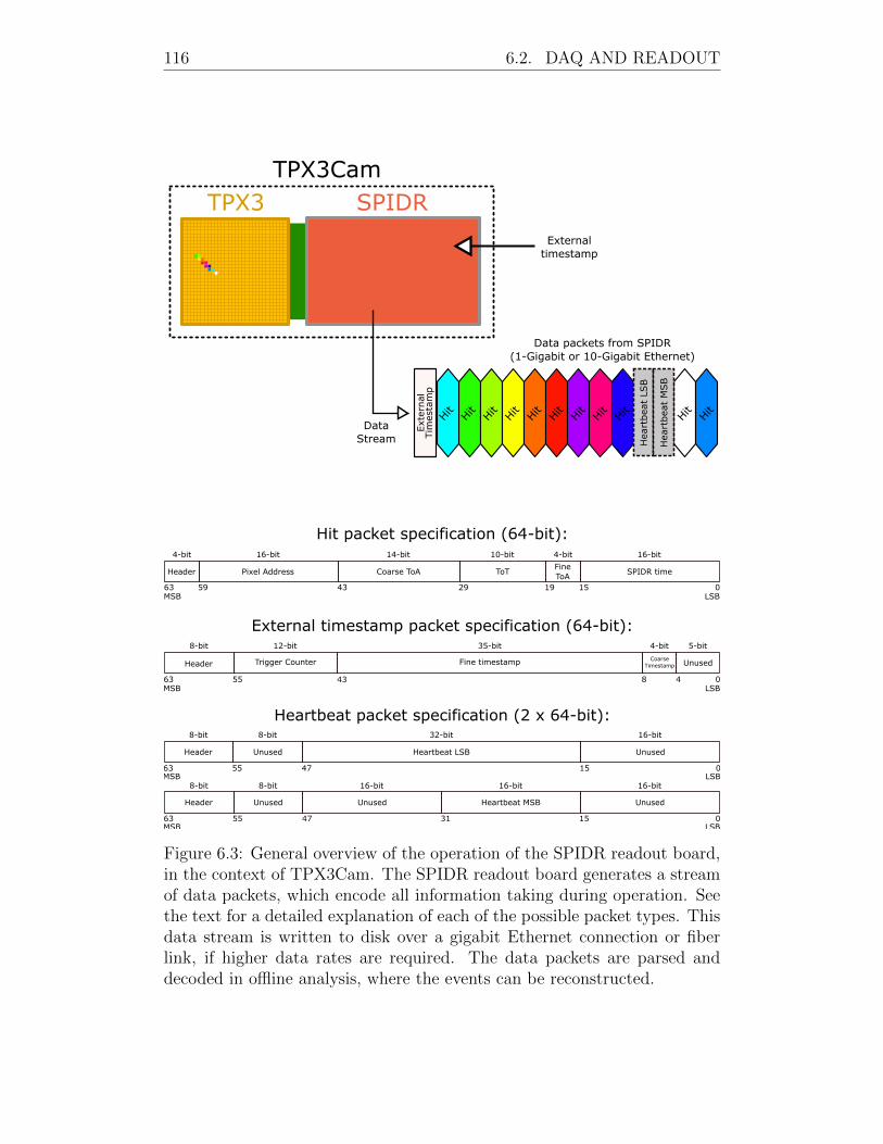
116 6.2. DAQ AND READOUT
TPX3 SPIDRTPX3Cam
DataStream
Data packets from SPIDR(1-Gigabit or 10-Gigabit Ethernet)
Hit packet specification (64-bit):
External timestamp packet specification (64-bit):
Heartbeat packet specification (2 x 64-bit):
Header
4-bit
Pixel Address
16-bit
Coarse ToA
14-bit 10-bit
ToT
4-bit
FineToA
SPIDR time
16-bit
LSBMSB151929435963 0
Header
8-bit
Unused
5-bit
LSBMSB5563 0
CoarseTimestamp
4-bit
Fine timestamp
35-bit
Trigger Counter
12-bit
43 48
Ext
ernal
Tim
esta
mp
Hit
Hit
Hit
Hit
Hit
Hit
Hit
Hit
Hit
Hit
Hit
Hea
rtbea
t LS
B
Hea
rtbea
t M
SB
Header
8-bit
Unused
LSBMSB63 0
Heartbeat LSB
16-bit
Unused
8-bit
1555 47
32-bit
Header
8-bit
Unused
LSBMSB63 0
Heartbeat MSB
16-bit
Unused
8-bit
1555 47 31
16-bit16-bit
Unused
External timestamp
Figure 6.3: General overview of the operation of the SPIDR readout board,in the context of TPX3Cam. The SPIDR readout board generates a streamof data packets, which encode all information taking during operation. Seethe text for a detailed explanation of each of the possible packet types. Thisdata stream is written to disk over a gigabit Ethernet connection or fiberlink, if higher data rates are required. The data packets are parsed anddecoded in offline analysis, where the events can be reconstructed.
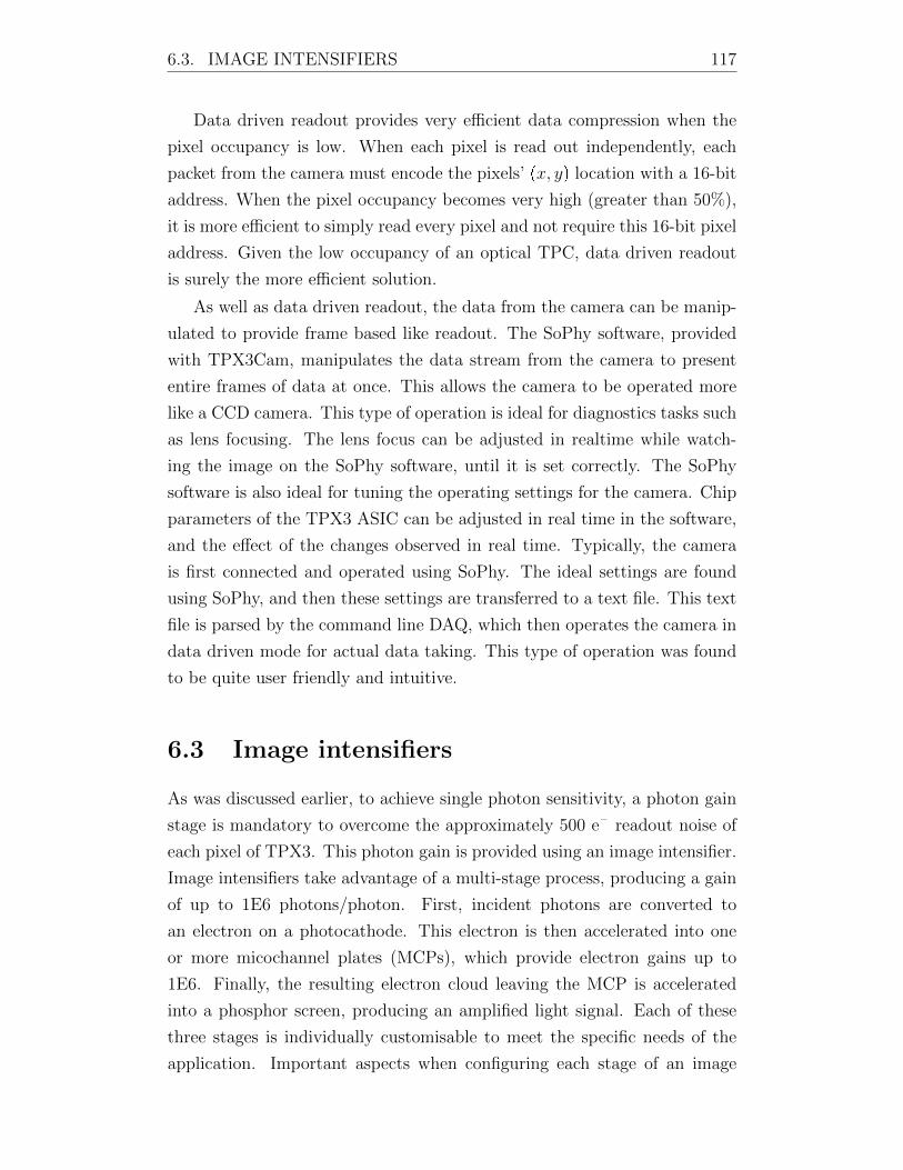
6.3. IMAGE INTENSIFIERS 117
Data driven readout provides very efficient data compression when the
pixel occupancy is low. When each pixel is read out independently, each
packet from the camera must encode the pixels’ px, yq location with a 16-bit
address. When the pixel occupancy becomes very high (greater than 50%),
it is more efficient to simply read every pixel and not require this 16-bit pixel
address. Given the low occupancy of an optical TPC, data driven readout
is surely the more efficient solution.
As well as data driven readout, the data from the camera can be manip-
ulated to provide frame based like readout. The SoPhy software, provided
with TPX3Cam, manipulates the data stream from the camera to present
entire frames of data at once. This allows the camera to be operated more
like a CCD camera. This type of operation is ideal for diagnostics tasks such
as lens focusing. The lens focus can be adjusted in realtime while watch-
ing the image on the SoPhy software, until it is set correctly. The SoPhy
software is also ideal for tuning the operating settings for the camera. Chip
parameters of the TPX3 ASIC can be adjusted in real time in the software,
and the effect of the changes observed in real time. Typically, the camera
is first connected and operated using SoPhy. The ideal settings are found
using SoPhy, and then these settings are transferred to a text file. This text
file is parsed by the command line DAQ, which then operates the camera in
data driven mode for actual data taking. This type of operation was found
to be quite user friendly and intuitive.
6.3 Image intensifiers
As was discussed earlier, to achieve single photon sensitivity, a photon gain
stage is mandatory to overcome the approximately 500 e– readout noise of
each pixel of TPX3. This photon gain is provided using an image intensifier.
Image intensifiers take advantage of a multi-stage process, producing a gain
of up to 1E6 photons/photon. First, incident photons are converted to
an electron on a photocathode. This electron is then accelerated into one
or more micochannel plates (MCPs), which provide electron gains up to
1E6. Finally, the resulting electron cloud leaving the MCP is accelerated
into a phosphor screen, producing an amplified light signal. Each of these
three stages is individually customisable to meet the specific needs of the
application. Important aspects when configuring each stage of an image
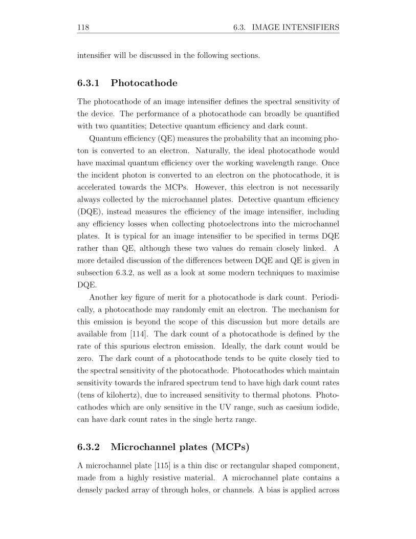
118 6.3. IMAGE INTENSIFIERS
intensifier will be discussed in the following sections.
6.3.1 Photocathode
The photocathode of an image intensifier defines the spectral sensitivity of
the device. The performance of a photocathode can broadly be quantified
with two quantities; Detective quantum efficiency and dark count.
Quantum efficiency (QE) measures the probability that an incoming pho-
ton is converted to an electron. Naturally, the ideal photocathode would
have maximal quantum efficiency over the working wavelength range. Once
the incident photon is converted to an electron on the photocathode, it is
accelerated towards the MCPs. However, this electron is not necessarily
always collected by the microchannel plates. Detective quantum efficiency
(DQE), instead measures the efficiency of the image intensifier, including
any efficiency losses when collecting photoelectrons into the microchannel
plates. It is typical for an image intensifier to be specified in terms DQE
rather than QE, although these two values do remain closely linked. A
more detailed discussion of the differences between DQE and QE is given in
subsection 6.3.2, as well as a look at some modern techniques to maximise
DQE.
Another key figure of merit for a photocathode is dark count. Periodi-
cally, a photocathode may randomly emit an electron. The mechanism for
this emission is beyond the scope of this discussion but more details are
available from [114]. The dark count of a photocathode is defined by the
rate of this spurious electron emission. Ideally, the dark count would be
zero. The dark count of a photocathode tends to be quite closely tied to
the spectral sensitivity of the photocathode. Photocathodes which maintain
sensitivity towards the infrared spectrum tend to have high dark count rates
(tens of kilohertz), due to increased sensitivity to thermal photons. Photo-
cathodes which are only sensitive in the UV range, such as caesium iodide,
can have dark count rates in the single hertz range.
6.3.2 Microchannel plates (MCPs)
A microchannel plate [115] is a thin disc or rectangular shaped component,
made from a highly resistive material. A microchannel plate contains a
densely packed array of through holes, or channels. A bias is applied across
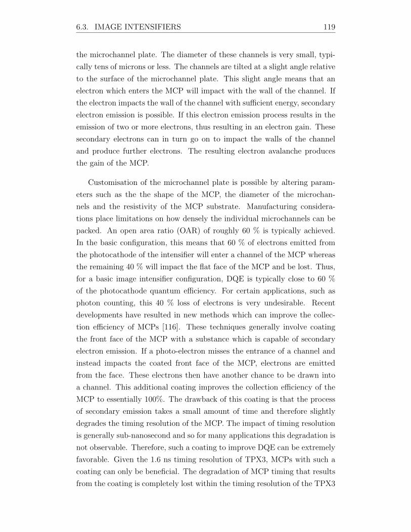
6.3. IMAGE INTENSIFIERS 119
the microchannel plate. The diameter of these channels is very small, typi-
cally tens of microns or less. The channels are tilted at a slight angle relative
to the surface of the microchannel plate. This slight angle means that an
electron which enters the MCP will impact with the wall of the channel. If
the electron impacts the wall of the channel with sufficient energy, secondary
electron emission is possible. If this electron emission process results in the
emission of two or more electrons, thus resulting in an electron gain. These
secondary electrons can in turn go on to impact the walls of the channel
and produce further electrons. The resulting electron avalanche produces
the gain of the MCP.
Customisation of the microchannel plate is possible by altering param-
eters such as the the shape of the MCP, the diameter of the microchan-
nels and the resistivity of the MCP substrate. Manufacturing considera-
tions place limitations on how densely the individual microchannels can be
packed. An open area ratio (OAR) of roughly 60 % is typically achieved.
In the basic configuration, this means that 60 % of electrons emitted from
the photocathode of the intensifier will enter a channel of the MCP whereas
the remaining 40 % will impact the flat face of the MCP and be lost. Thus,
for a basic image intensifier configuration, DQE is typically close to 60 %
of the photocathode quantum efficiency. For certain applications, such as
photon counting, this 40 % loss of electrons is very undesirable. Recent
developments have resulted in new methods which can improve the collec-
tion efficiency of MCPs [116]. These techniques generally involve coating
the front face of the MCP with a substance which is capable of secondary
electron emission. If a photo-electron misses the entrance of a channel and
instead impacts the coated front face of the MCP, electrons are emitted
from the face. These electrons then have another chance to be drawn into
a channel. This additional coating improves the collection efficiency of the
MCP to essentially 100%. The drawback of this coating is that the process
of secondary emission takes a small amount of time and therefore slightly
degrades the timing resolution of the MCP. The impact of timing resolution
is generally sub-nanosecond and so for many applications this degradation is
not observable. Therefore, such a coating to improve DQE can be extremely
favorable. Given the 1.6 ns timing resolution of TPX3, MCPs with such a
coating can only be beneficial. The degradation of MCP timing that results
from the coating is completely lost within the timing resolution of the TPX3
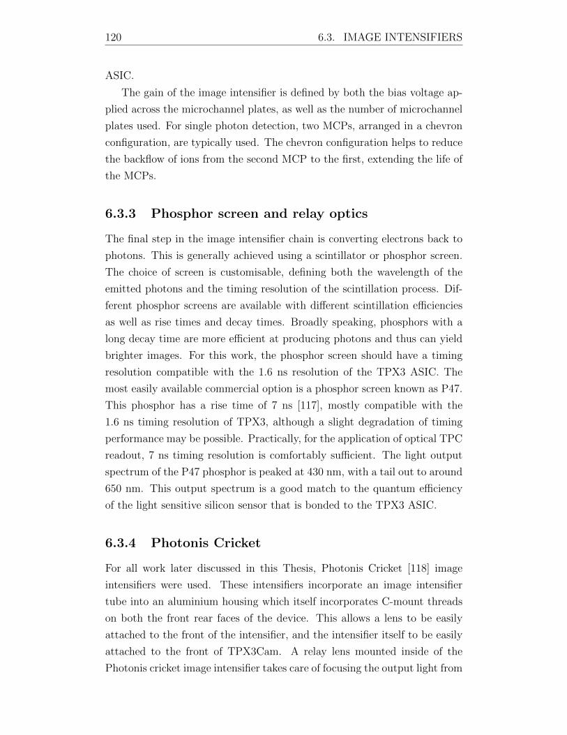
120 6.3. IMAGE INTENSIFIERS
ASIC.
The gain of the image intensifier is defined by both the bias voltage ap-
plied across the microchannel plates, as well as the number of microchannel
plates used. For single photon detection, two MCPs, arranged in a chevron
configuration, are typically used. The chevron configuration helps to reduce
the backflow of ions from the second MCP to the first, extending the life of
the MCPs.
6.3.3 Phosphor screen and relay optics
The final step in the image intensifier chain is converting electrons back to
photons. This is generally achieved using a scintillator or phosphor screen.
The choice of screen is customisable, defining both the wavelength of the
emitted photons and the timing resolution of the scintillation process. Dif-
ferent phosphor screens are available with different scintillation efficiencies
as well as rise times and decay times. Broadly speaking, phosphors with a
long decay time are more efficient at producing photons and thus can yield
brighter images. For this work, the phosphor screen should have a timing
resolution compatible with the 1.6 ns resolution of the TPX3 ASIC. The
most easily available commercial option is a phosphor screen known as P47.
This phosphor has a rise time of 7 ns [117], mostly compatible with the
1.6 ns timing resolution of TPX3, although a slight degradation of timing
performance may be possible. Practically, for the application of optical TPC
readout, 7 ns timing resolution is comfortably sufficient. The light output
spectrum of the P47 phosphor is peaked at 430 nm, with a tail out to around
650 nm. This output spectrum is a good match to the quantum efficiency
of the light sensitive silicon sensor that is bonded to the TPX3 ASIC.
6.3.4 Photonis Cricket
For all work later discussed in this Thesis, Photonis Cricket [118] image
intensifiers were used. These intensifiers incorporate an image intensifier
tube into an aluminium housing which itself incorporates C-mount threads
on both the front rear faces of the device. This allows a lens to be easily
attached to the front of the intensifier, and the intensifier itself to be easily
attached to the front of TPX3Cam. A relay lens mounted inside of the
Photonis cricket image intensifier takes care of focusing the output light from
6.3. IMAGE INTENSIFIERS 121
the phosphor screen of the intensifier onto the silicon sensor of TPX3Cam.
A focus wheel is provided, allowing fine adjustment of the focal point of the
relay optics.
The Photonis cricket intensifier has a built in power supply with over
current protection. In case that the intensifier is exposed to bright light,
the voltage across the MCPs is reduced to protect both the MCP and the
phosphor screen. The cricket is powered using a basic, low voltage, micro-
usb cable. The internal power supply converts the usb voltage into the high
voltage required by the intensifier. The cricket additionally has a LEMO
connector, which can be used to regulate the gain of the intensifier by ap-
plying an external voltage. When no voltage is applied to this connector, the
gain of the MCP is maximum. Up to 5V can be applied to this connector,
reducing the gain of the intensifier by at least 100 times. For this work,
the intensifier was always used at maximum gain. The Photonis Cricket
was found to be very user friendly and provided essentially plug and play
capability.
Chapter 7
Performance of optical TPX3
readout in 100 mbar CF4 gas
This section is an expanded discussion surrounding the work published in
[119].
After returning from CERN, the ARIADNE detector was unavailable due
to a period of maintenance and upgrade. The first attempt at Timepix based
optical readout was therefore performed using a smaller secondary TPC. The
ARIADNE demonstrator is a 40 liter TPC, which has in the past been used
for tests using CCD and EMCCD cameras [95, 120]. The smaller size of the
demonstrator TPC makes it more practical for certain R&D activities; The
smaller detector volume makes exchanging gas mixtures possible in a much
shorter time frame.
7.0.1 Intensifier configuration
A Photonis cricket intensifier was used for these tests. The intensifier had
a Photonis Hi-QE Red photocathode. This photocathode has a quantum
efficiency of 20% at 620 nm, the peak scintillation wavelength of CF4 of
620 nm. One drawback of the Hi-QE Red photocathode is the relatively high
dark count. The dark count rate of the photocathode is in the range 30-60
kHz. The intensifier has two MCPs, arranged in a chevron configuration
with a total electron gain of 85 000 and an output brightness of 1.8 cd/m2.
The output screen is a P47 phosphor. Figure 7.1 shows a photograph of the
camera, with the image intensifier and lens attached. A lens cap is installed
122
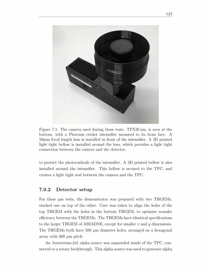
123
Figure 7.1: The camera used during these tests. TPX3Cam, is seen at thebottom, with a Photonis cricket intensifier mounted to its front face. A50mm focal length lens is installed in front of the intensifier. A 3D printedlight tight bellow is installed around the lens, which provides a light tightconnection between the camera and the detector.
to protect the photocathode of the intensifier. A 3D printed bellow is also
installed around the intensifier. This bellow is secured to the TPC, and
creates a light tight seal between the camera and the TPC.
7.0.2 Detector setup
For these gas tests, the demonstrator was prepared with two THGEMs,
stacked one on top of the other. Care was taken to align the holes of the
top THGEM with the holes in the bottom THGEM, to optimise transfer
efficiency between the THGEMs. The THGEMs have identical specifications
to the larger THGEM of ARIADNE, except for smaller x and y dimensions.
The THGEMs both have 500 µm diameter holes, arranged on a hexagonal
array with 800 µm pitch.
An Americium-241 alpha source was suspended inside of the TPC, con-
nected to a rotary feedthrough. This alpha source was used to generate alpha
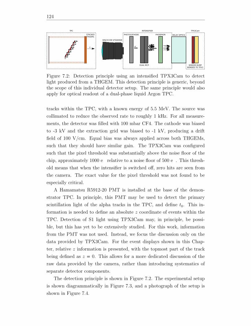
124
PHOTOCATHODE
DUAL MCP
e-
PHOSPHOR
INTENSIFIER
STACKEDTHGEMs
γ
TPC
e-
TPX3Cam
SENSOR BUMP BONDED TO TPX3
RELAY OPTICS
SPACECOM VF50095M
Figure 7.2: Detection principle using an intensified TPX3Cam to detectlight produced from a THGEM. This detection principle is generic, beyondthe scope of this individual detector setup. The same principle would alsoapply for optical readout of a dual-phase liquid Argon TPC.
tracks within the TPC, with a known energy of 5.5 MeV. The source was
collimated to reduce the observed rate to roughly 1 kHz. For all measure-
ments, the detector was filled with 100 mbar CF4. The cathode was biased
to -3 kV and the extraction grid was biased to -1 kV, producing a drift
field of 100 V/cm. Equal bias was always applied across both THGEMs,
such that they should have similar gain. The TPX3Cam was configured
such that the pixel threshold was substantially above the noise floor of the
chip, approximately 1000 e relative to a noise floor of 500 e. This thresh-
old means that when the intensifier is switched off, zero hits are seen from
the camera. The exact value for the pixel threshold was not found to be
especially critical.
A Hamamatsu R5912-20 PMT is installed at the base of the demon-
strator TPC. In principle, this PMT may be used to detect the primary
scintillation light of the alpha tracks in the TPC, and define t0. This in-
formation is needed to define an absolute z coordinate of events within the
TPC. Detection of S1 light using TPX3Cam may, in principle, be possi-
ble, but this has yet to be extensively studied. For this work, information
from the PMT was not used. Instead, we focus the discussion only on the
data provided by TPX3Cam. For the event displays shown in this Chap-
ter, relative z information is presented, with the topmost part of the track
being defined as z 0. This allows for a more dedicated discussion of the
raw data provided by the camera, rather than introducing systematics of
separate detector components.
The detection principle is shown in Figure 7.2. The experimental setup
is shown diagrammatically in Figure 7.3, and a photograph of the setup is
shown in Figure 7.4.
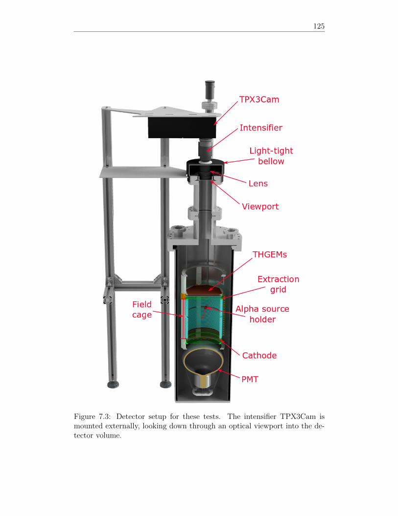
125
Figure 7.3: Detector setup for these tests. The intensifier TPX3Cam ismounted externally, looking down through an optical viewport into the de-tector volume.
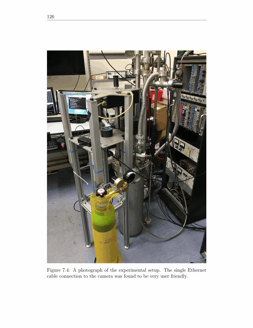
126
Figure 7.4: A photograph of the experimental setup. The single Ethernetcable connection to the camera was found to be very user friendly.
127
7.0.3 Results
As discussed in 6.2, we can consider two types of data readout. Firstly,
there is readout using SoPhy. SoPhy manipulates the data stream from
TPX3Cam, emulating a camera with a traditional frame based readout.
By integrating all hits within a specified time window, a single image is
produced with a simulated exposure time. This type of readout is ideal
for basic diagnostic tasks, such as focusing the lens of the camera. This
software was used to initially asses the sensitivity of the camera to the light
produced in the TPC, and get a rough feel for the performance of the device.
Figures 7.5 and 7.6 shows event displays taken using SoPhy, for two different
exposure settings. Two separate views are seen, one is time over threshold
(intensity) and the other is time of arrival. From these initial observations
in SoPhy, it was possible to draw several initial conclusions. First, each
track is seen to have a clear Bragg peak. This give a promising outlook
for the calorimetric performance of the camera. Secondly, each alpha track
is clearly resolved from one another in time, shown by each track having a
different colour in ToA mode. Moreover, when we adjust the colour scale to
focus on a single alpha track, changing timing information along the length
of the track is visible. Since the drift velocity in a TPC is know, this timing
information along the length of the track can be used to perform a full 3D
track reconstruction in (x,y,z). Considering the extremely fast drift velocity
of 10 cm/µs in 100 mbar CF4, compared to 0.16 cm/µs in Liquid Argon,
this was a critical success. It was clear early on during experimentation in
SoPhy that the timing resolution of the camera was more than sufficient for
the application of optical TPC readout.
In the event displays, a halo of hits can be seen around each image. This
halo is caused by the field of view of the camera being wider than required.
Reflections from the stainless steel nipple, leading up from the THGEM to
the camera, are seen by the camera. This lens gives the camera a larger field
of view than is required for these measurements. These reflections would
not be present when using properly configured optics. These tests were
deliberately performed with this excessive field of view, using the Spacecom
VF50095M lens, so that results may be easily interpreted in the context of
ARIADNE, where this lens is used by the EMCCD cameras.
Once the camera had been reasonably configured using SoPhy, data was
taken using the data driven command line DAQ. This results in the creation
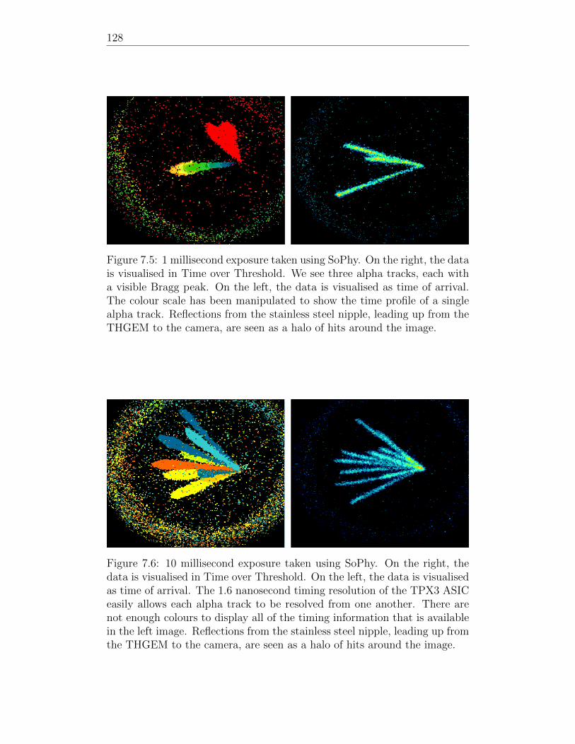
128
Figure 7.5: 1 millisecond exposure taken using SoPhy. On the right, the datais visualised in Time over Threshold. We see three alpha tracks, each witha visible Bragg peak. On the left, the data is visualised as time of arrival.The colour scale has been manipulated to show the time profile of a singlealpha track. Reflections from the stainless steel nipple, leading up from theTHGEM to the camera, are seen as a halo of hits around the image.
Figure 7.6: 10 millisecond exposure taken using SoPhy. On the right, thedata is visualised in Time over Threshold. On the left, the data is visualisedas time of arrival. The 1.6 nanosecond timing resolution of the TPX3 ASICeasily allows each alpha track to be resolved from one another. There arenot enough colours to display all of the timing information that is availablein the left image. Reflections from the stainless steel nipple, leading up fromthe THGEM to the camera, are seen as a halo of hits around the image.
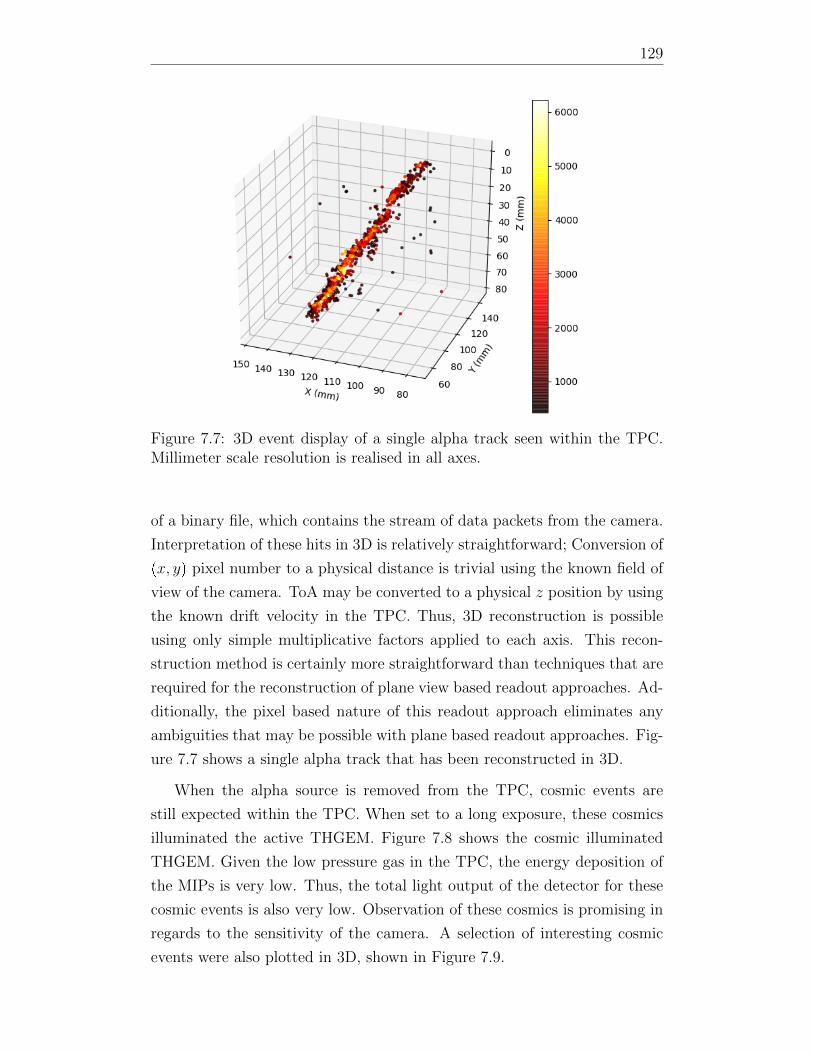
129
Figure 7.7: 3D event display of a single alpha track seen within the TPC.Millimeter scale resolution is realised in all axes.
of a binary file, which contains the stream of data packets from the camera.
Interpretation of these hits in 3D is relatively straightforward; Conversion of
px, yq pixel number to a physical distance is trivial using the known field of
view of the camera. ToA may be converted to a physical z position by using
the known drift velocity in the TPC. Thus, 3D reconstruction is possible
using only simple multiplicative factors applied to each axis. This recon-
struction method is certainly more straightforward than techniques that are
required for the reconstruction of plane view based readout approaches. Ad-
ditionally, the pixel based nature of this readout approach eliminates any
ambiguities that may be possible with plane based readout approaches. Fig-
ure 7.7 shows a single alpha track that has been reconstructed in 3D.
When the alpha source is removed from the TPC, cosmic events are
still expected within the TPC. When set to a long exposure, these cosmics
illuminated the active THGEM. Figure 7.8 shows the cosmic illuminated
THGEM. Given the low pressure gas in the TPC, the energy deposition of
the MIPs is very low. Thus, the total light output of the detector for these
cosmic events is also very low. Observation of these cosmics is promising in
regards to the sensitivity of the camera. A selection of interesting cosmic
events were also plotted in 3D, shown in Figure 7.9.
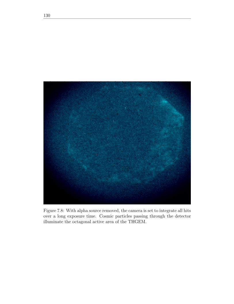
130
Figure 7.8: With alpha source removed, the camera is set to integrate all hitsover a long exposure time. Cosmic particles passing through the detectorilluminate the octagonal active area of the THGEM.
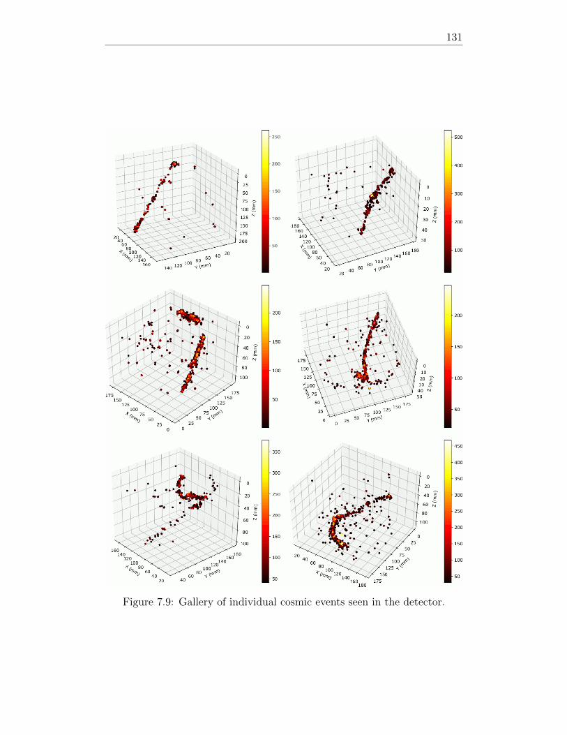
131
Figure 7.9: Gallery of individual cosmic events seen in the detector.
132
7.0.4 THGEM Bias scan
The response of the camera to changing THGEM bias was studied. For
a single THGEM, the light production in a THGEM can be decomposed
into a linear and exponential components. With inccreasing bias across the
THGEM, the light production of the THGEM also increases. This means
that more photons should reach the camera. This should, in turn, lead to
an increasing number of hits seen by the camera. If we plot the camera
hit rate versus THGEM bias, we can measure light production. Figure 7.10
shows the hit rate of the camera as a function of THGEM bias. In this
Figure, a single exponential function has been used to fit the data. The
theoretical model predicted in Section 3 does not fit the data well. This is
most likely due to this setup having a double THGEM setup, whereas the
proposed function is only appropriate for a single THGEM. Nevertheless, a
single exponential function provides a decent description of the data.
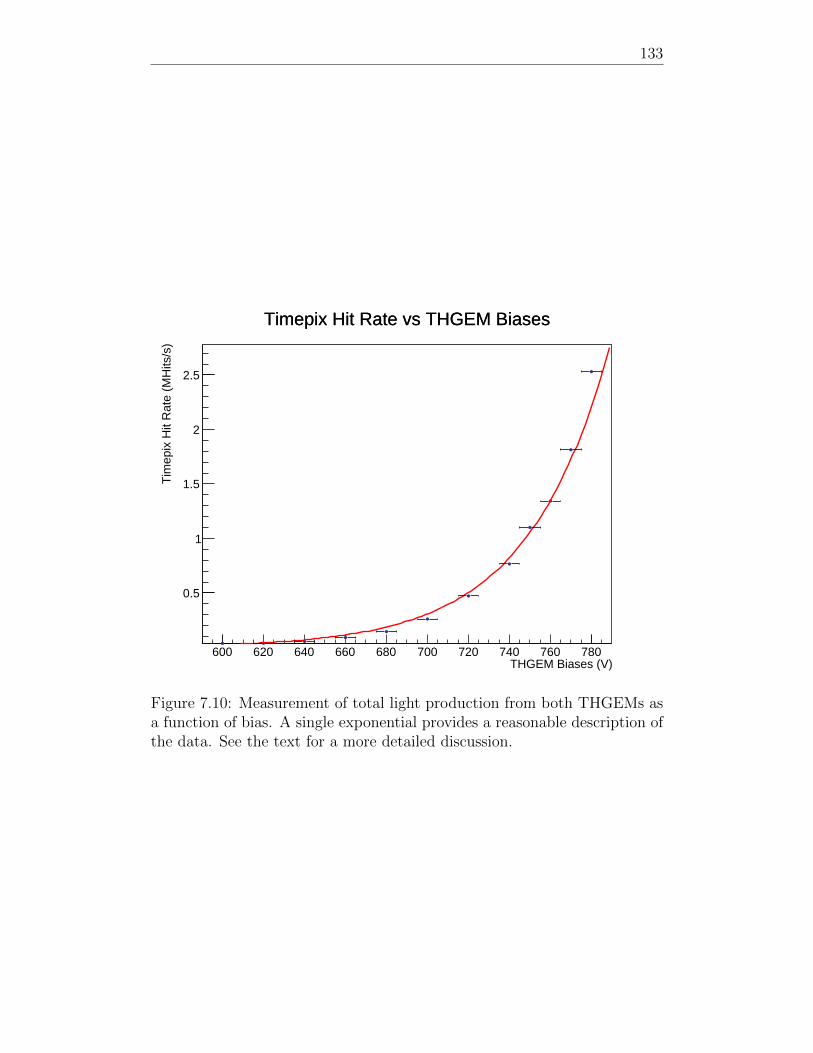
133
600 620 640 660 680 700 720 740 760 780THGEM Biases (V)
0.5
1
1.5
2
2.5
Tim
epix
Hit
Rat
e (M
Hits
/s)
Timepix Hit Rate vs THGEM BiasesTimepix Hit Rate vs THGEM Biases
Figure 7.10: Measurement of total light production from both THGEMs asa function of bias. A single exponential provides a reasonable description ofthe data. See the text for a more detailed discussion.
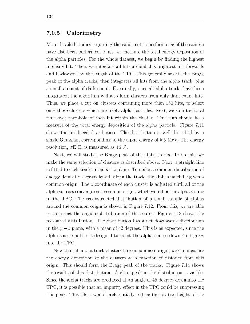
134
7.0.5 Calorimetry
More detailed studies regarding the calorimetric performance of the camera
have also been performed. First, we measure the total energy deposition of
the alpha particles. For the whole dataset, we begin by finding the highest
intensity hit. Then, we integrate all hits around this brightest hit, forwards
and backwards by the length of the TPC. This generally selects the Bragg
peak of the alpha tracks, then integrates all hits from the alpha track, plus
a small amount of dark count. Eventually, once all alpha tracks have been
integrated, the algorithm will also form clusters from only dark count hits.
Thus, we place a cut on clusters containing more than 160 hits, to select
only those clusters which are likely alpha particles. Next, we sum the total
time over threshold of each hit within the cluster. This sum should be a
measure of the total energy deposition of the alpha particle. Figure 7.11
shows the produced distribution. The distribution is well described by a
single Gaussian, corresponding to the alpha energy of 5.5 MeV. The energy
resolution, σEE, is measured as 16 %.
Next, we will study the Bragg peak of the alpha tracks. To do this, we
make the same selection of clusters as described above. Next, a straight line
is fitted to each track in the y z plane. To make a common distribution of
energy deposition versus length along the track, the alphas much be given a
common origin. The z coordinate of each cluster is adjusted until all of the
alpha sources converge on a common origin, which would be the alpha source
in the TPC. The reconstructed distribution of a small sample of alphas
around the common origin is shown in Figure 7.12. From this, we are able
to construct the angular distribution of the source. Figure 7.13 shows the
measured distribution. The distribution has a net downwards distribution
in the y z plane, with a mean of 42 degrees. This is as expected, since the
alpha source holder is designed to point the alpha source down 45 degrees
into the TPC.
Now that all alpha track clusters have a common origin, we can measure
the energy deposition of the clusters as a function of distance from this
origin. This should form the Bragg peak of the tracks. Figure 7.14 shows
the results of this distribution. A clear peak in the distribution is visible.
Since the alpha tracks are produced at an angle of 45 degrees down into the
TPC, it is possible that an impurity effect in the TPC could be suppressing
this peak. This effect would preferentially reduce the relative height of the
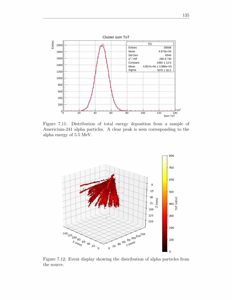
135
h1Entries 39598Mean 4.873e+04Std Dev 8344
/ ndf 2χ 290.9 / 90Constant 12.6± 1992 Mean 3.986e+01± 4.857e+04 Sigma 30.2± 7876
0 20 40 60 80 100 120 140
310×
Sum ToT
0
200
400
600
800
1000
1200
1400
1600
1800
2000
Ent
ries
h1Entries 39598Mean 4.873e+04Std Dev 8344
/ ndf 2χ 290.9 / 90Constant 12.6± 1992 Mean 3.986e+01± 4.857e+04 Sigma 30.2± 7876
Cluster sum ToT
Figure 7.11: Distribution of total energy deposition from a sample ofAmericium-241 alpha particles. A clear peak is seen corresponding to thealpha energy of 5.5 MeV.
Figure 7.12: Event display showing the distribution of alpha particles fromthe source.
136
peak, since electrons from the Bragg peak of the track have to drift further
in the TPC. Future work will attempt to quantify this impurity effect. If
this impurity effect is present and corrected for, the alpha energy resolution
shown in Figure 7.11 may also be improved.
7.0.6 Discussion
The initial performance of TPX3Cam in these gas tests was very promis-
ing. The most critical benefit is that full px, y, z, Eq tracking is now possible
using a single device. Alongside this however, TPX3 also delivered many
additional benefits. The native 3D data format provided to be very con-
venient. The simplicity of 3D reconstruction using a single multiplicative
factor on each axis greatly simplified analysis efforts. Moreover, the zero
suppressed nature of the data provided very clean events in 3D. This raw
data format was ideal for analysis tasks such as straight line fitting and
clustering. In the past, using EMCCDs, initial pre-filtering was required to
remove background pixels from the raw data, which inevitably introduced
inefficiencies.
The zero-suppressed nature of the raw data was additionally found to
produce very low data rates from the camera. Each hit from the camera is
defined using 64 bits. The alpha tracks are generally formed by 1000 hits or
less. Thus, each track is fully defined with Op10 kilobytesq. Given the source
rate of 1 kHz, the total hit rate from the camera is roughly 1 Mhits/s. This
is far from the maximum bandwidth of 80 MHits/s that is possible using the
SPIDR readout board. It was clear that the camera would have no readout
difficulty, even in high pileup environments.
The triggerless nature of the readout was also a novel component of this
camera. The decoupling of the camera from the trigger system meant that
any inefficiencies in trigger selection can not introduce bias into the raw
data. The camera streams all data from the TPC, and comparison of the
data to the trigger timestamps is done offline in analysis. In case that a
trigger bias does exist, this can be understood and corrected offline. The
triggering configuration never effects the raw data stream from the camera,
and thus the raw data can never become unintentionally biased.
Before these tests were performed, it was unclear if the timing resolution
of the TPX3 ASIC would be sufficient for high resolution z axis reconstruc-
tion in gas TPCs, where the drift velocity is much faster than Liquid Argon.
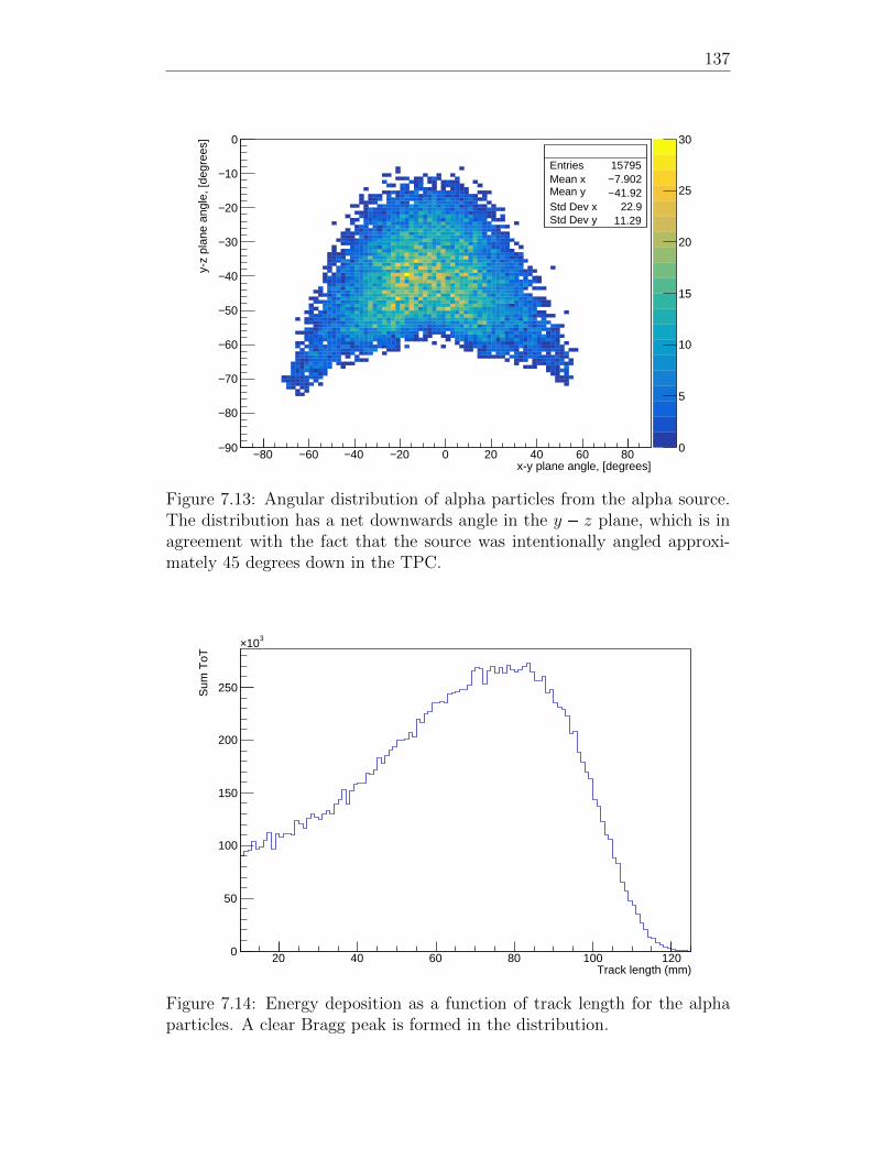
137
80− 60− 40− 20− 0 20 40 60 80x-y plane angle, [degrees]
90−
80−
70−
60−
50−
40−
30−
20−
10−
0
y-z
plan
e an
gle,
[deg
rees
]
Entries 15795Mean x 7.902− Mean y 41.92− Std Dev x 22.9Std Dev y 11.29
0
5
10
15
20
25
30
Entries 15795Mean x 7.902− Mean y 41.92− Std Dev x 22.9Std Dev y 11.29
Figure 7.13: Angular distribution of alpha particles from the alpha source.The distribution has a net downwards angle in the y z plane, which is inagreement with the fact that the source was intentionally angled approxi-mately 45 degrees down in the TPC.
20 40 60 80 100 120Track length (mm)
0
50
100
150
200
250
310×
Sum
ToT
Figure 7.14: Energy deposition as a function of track length for the alphaparticles. A clear Bragg peak is formed in the distribution.

138
In fact, this work found that the timing resolution was easily sufficient for
millimeter scale resolution in the z axis. It may be conceivable to read-
out high pressure gas TPCs using this technology, provided sufficient light
production is possible.
Chapter 8
Performance of optical TPX3
readout in Liquid Argon
Following the successful demonstration in gas, a TPX3 camera was installed
onto the ARIADNE detector to perform a Liquid Argon demonstration.
For this demonstration, a Photonis cricket image intensifier was used, as
described in Section 6.3.4. The intensifier has a Photonis Hi-QE Green pho-
tocathode, with a quantum efficiency of 30 % at 430 nm, the peak emission
wavelength of TPB. The dark count rate of this photocathode is 50 Hz,
orders of magnitude less than that of the photocathode used in the gas
demonstration. For these measurements, a trigger timestamp, generated by
the internal PMTs, was supplied to the camera. This allowed the absolute
z position of the tracks in the TPC to be determined by measuring the time
difference between S1 and S2 signals. Figure 8.1 shows the camera installed
onto the ARIADNE detector.
139
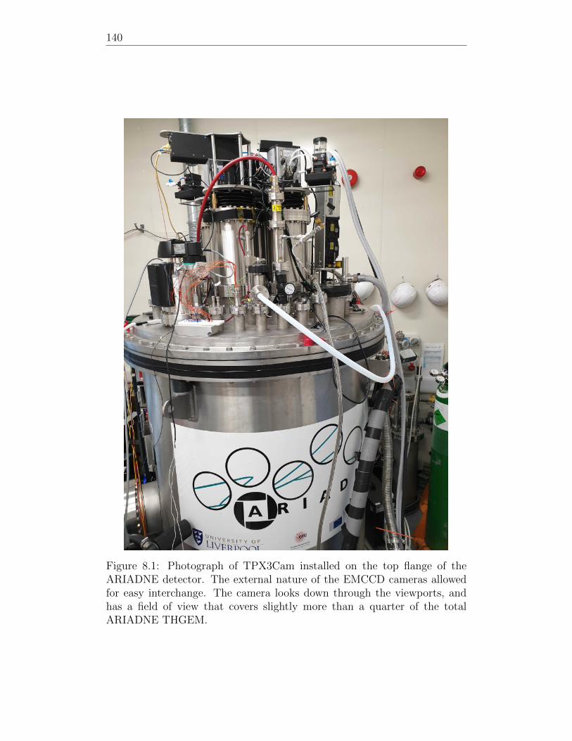
140
Figure 8.1: Photograph of TPX3Cam installed on the top flange of theARIADNE detector. The external nature of the EMCCD cameras allowedfor easy interchange. The camera looks down through the viewports, andhas a field of view that covers slightly more than a quarter of the totalARIADNE THGEM.
8.1. GALLERY 141
8.1 Gallery
The performance of the camera was first assessed using the diagnostic soft-
ware SoPhy. Figures 8.2 and 8.3 show several screenshots taking using the
SoPhy software, in both time over threshold and time of arrival modes. The
brightness of the cosmic muons is seen to decrease with depth in the TPC,
due to losses to electronegative impurities. In fact, a detailed measurement
of this effect allows for a determination of electron lifetime. This is discussed
further in Section 8.3. Several point-like events are visible in the galleries,
which are background Gamma interactions, believed to be caused by 39Ar.
Data was also taken using the full Timepix3 DAQ, which provides simul-
taneous ToT and ToA. Figures 8.4 through 8.6 present a gallery of sample
events, reconstructed in 3D. The absolute z position of each event was de-
termined by comparison with the PMT trigger timestamp, t0. By measuring
the delay in time between the PMT t0 timestamp and the time of arrival
timestamp of the muon track signals, the z depth of the track in the TPC
may be determined. This time difference is converted to a physical distance
using the known drift velocity in the TPC. px, yq pixel number was converted
to mm using the known field of view of the camera, as determined from the
earlier gas tests. The z position was converted from the time to distance
using the known drift velocity in the TPC. The first four events show cos-
mic muons with a range of different delta rays. The last two events are two
stopping muon candidates. In both stopping muon events, a Bragg peak
at the end of the stopping muon track is visible, along with the produced
Michel Electron.
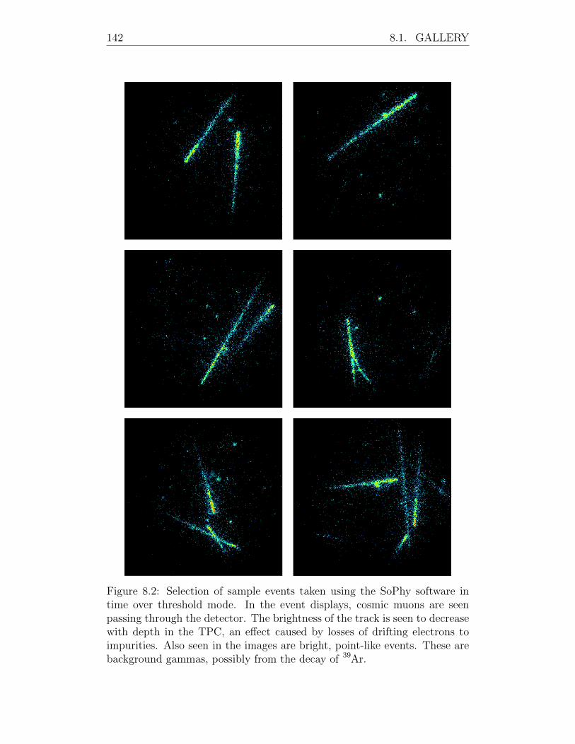
142 8.1. GALLERY
Figure 8.2: Selection of sample events taken using the SoPhy software intime over threshold mode. In the event displays, cosmic muons are seenpassing through the detector. The brightness of the track is seen to decreasewith depth in the TPC, an effect caused by losses of drifting electrons toimpurities. Also seen in the images are bright, point-like events. These arebackground gammas, possibly from the decay of 39Ar.
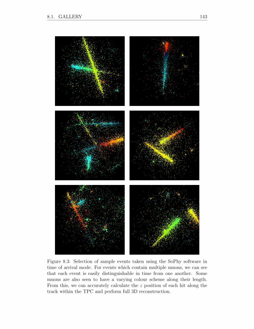
8.1. GALLERY 143
Figure 8.3: Selection of sample events taken using the SoPhy software intime of arrival mode. For events which contain multiple muons, we can seethat each event is easily distinguishable in time from one another. Somemuons are also seen to have a varying colour scheme along their length.From this, we can accurately calculate the z position of each hit along thetrack within the TPC and perform full 3D reconstruction.
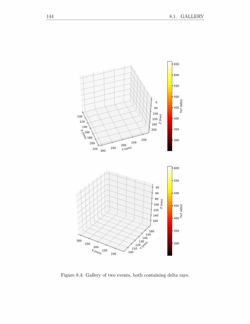
144 8.1. GALLERY
X (mm
)
100120
140160
180200
220 Y (mm)
100150
200250
300
Z (m
m)
0
50100150200250
300
350
400
450
500
550
600
650
ToT
(ADU
)
X (mm) 100150
200250
300
Y (mm)
100110
120130
140150
160
Z (m
m)
40
60
80100120140160
300
350
400
450
500
550
600
ToT
(ADU
)
Figure 8.4: Gallery of two events, both containing delta rays.
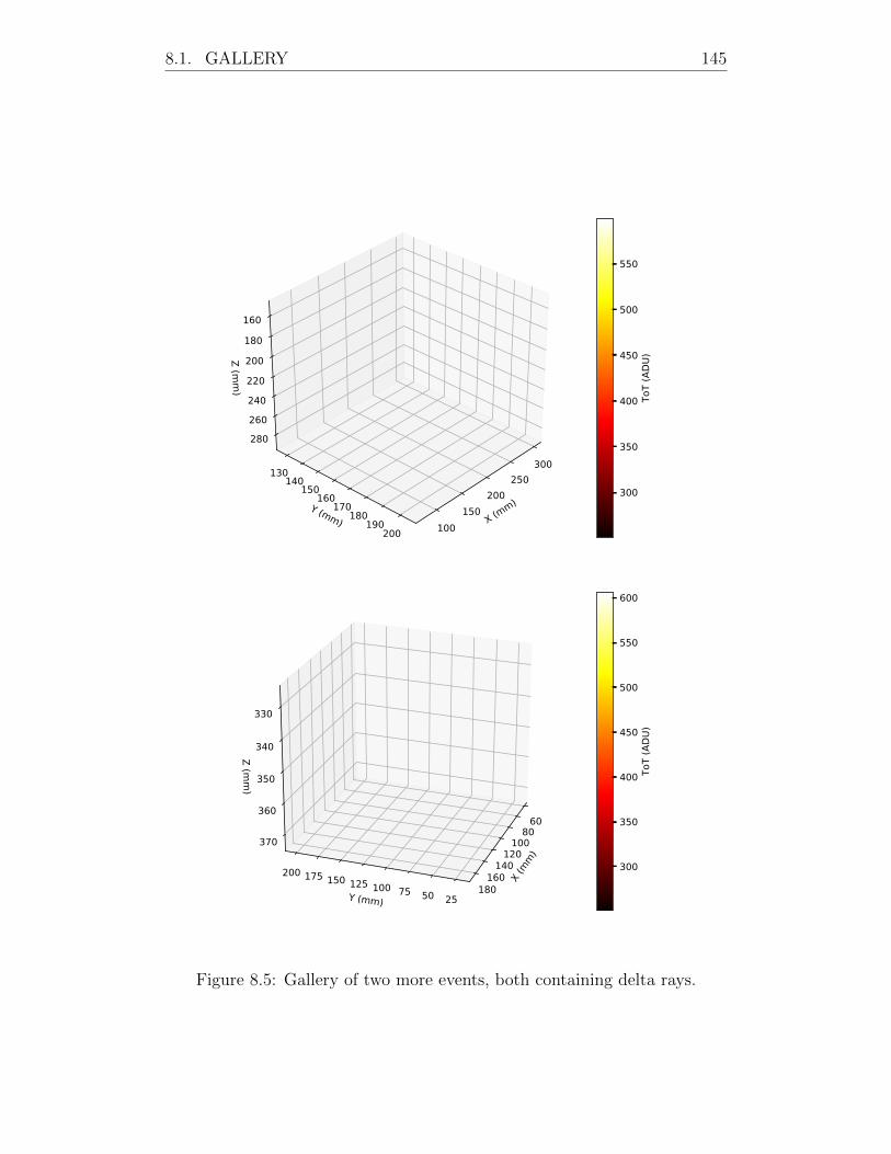
8.1. GALLERY 145
X (mm)
100150
200250
300
Y (mm)
130140
150160
170180
190200
Z (mm
)
160
180
200220240260280
300
350
400
450
500
550
ToT
(ADU
)
X (mm)
6080
100120
140160
180Y (mm) 255075100125150175200
Z (mm
)
330
340
350
360
370
300
350
400
450
500
550
600
ToT
(ADU
)
Figure 8.5: Gallery of two more events, both containing delta rays.
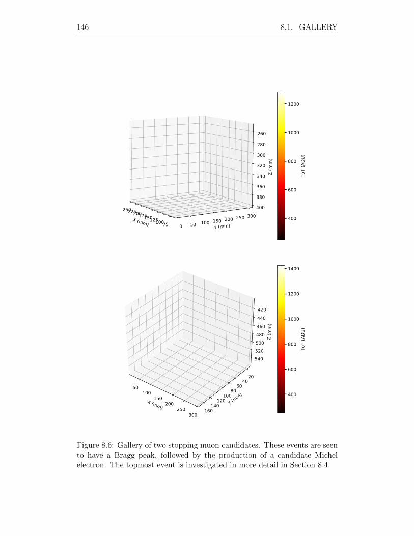
146 8.1. GALLERY
X (mm) 75100125150175200225250
Y (mm)0 50 100 150 200 250 300
Z (m
m)
260
280
300
320
340
360
380
400
400
600
800
1000
1200
ToT
(ADU
)
X (mm)
50100
150200
250300
Y (mm)
2040
6080
100120
140160
Z (m
m)
420440460480500520540
400
600
800
1000
1200
1400
ToT
(ADU
)
Figure 8.6: Gallery of two stopping muon candidates. These events are seento have a Bragg peak, followed by the production of a candidate Michelelectron. The topmost event is investigated in more detail in Section 8.4.
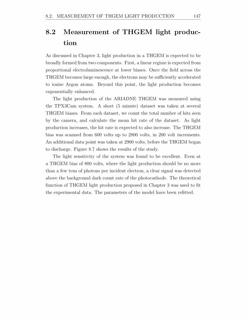
8.2. MEASUREMENT OF THGEM LIGHT PRODUCTION 147
8.2 Measurement of THGEM light produc-
tion
As discussed in Chapter 3, light production in a THGEM is expected to be
broadly formed from two components. First, a linear regime is expected from
proportional electroluminescence at lower biases. Once the field across the
THGEM becomes large enough, the electrons may be sufficiently accelerated
to ionise Argon atoms. Beyond this point, the light production becomes
exponentially enhanced.
The light production of the ARIADNE THGEM was measured using
the TPX3Cam system. A short (5 minute) dataset was taken at several
THGEM biases. From each dataset, we count the total number of hits seen
by the camera, and calculate the mean hit rate of the dataset. As light
production increases, the hit rate is expected to also increase. The THGEM
bias was scanned from 600 volts up to 2800 volts, in 200 volt increments.
An additional data point was taken at 2900 volts, before the THGEM began
to discharge. Figure 8.7 shows the results of the study.
The light sensitivity of the system was found to be excellent. Even at
a THGEM bias of 800 volts, where the light production should be no more
than a few tens of photons per incident electron, a clear signal was detected
above the background dark count rate of the photocathode. The theoretical
function of THGEM light production proposed in Chapter 3 was used to fit
the experimental data. The parameters of the model have been refitted.
148 8.2. MEASUREMENT OF THGEM LIGHT PRODUCTION
500 1000 1500 2000 2500 3000THGEM Potential Difference [V]
5000
10000
15000
20000
25000
Hit
rate
, [H
its/s
]
/ ndf 2χ 25.38 / 9p0 05− 8.703e± 0.003317 p1 0.03727± 0.8263 p2 32.97±355.9 − p3 0.0001776± 0.0006468
/ ndf 2χ 25.38 / 9p0 05− 8.703e± 0.003317 p1 0.03727± 0.8263 p2 32.97±355.9 − p3 0.0001776± 0.0006468
Figure 8.7: Measured light production of the ARIADNE THGEM as afunction of bias. The data is well described by a function of the formp1xp1 p3exppp0xqq p2.
8.3. MEASURING ELECTRON LIFETIME 149
8.3 Measuring electron lifetime
As electron drift time increases, the probability that the electron may en-
counter an impurity and be captured also increases. This results in the in-
tensity of MIPs being observed to reduce with increasing depth in the TPC.
Since throughgoing MIPs should have a generally uniform energy deposition
along their path length, they can be used as kind of a standard candle. By
measuring the track intensity versus depth in the TPC, the electron lifetime
may be determined.
In this study, a selection was made on MIPs which pass through the
THGEM. For these MIPs, we measure the track intensity as a function of
drift time, or depth in the TPC. This process is repeated for many MIPs
until an average distribution is formed. An exponential is fitted to this
distribution to determine electron lifetime. The method for event selection
is as follows;
1. Raw data is composed of both hits from TPX3Cam and trigger times-
tamp signals from the PMT. Trigger timestamp signals are assumed
to correspond to S1 (t0).
2. For each PMT trigger timestamp t0, collect all hits between t0 and
t0 550 µs (maximum ARIADNE drift length).
3. Cut those events which contain less than 1000 hits. This cut broadly
selects track-like events.
4. Perform a robust linear fit 1 in both x-z and y-z planes. The R-Squared
value must be ¡ 0.8 in both planes. Combine these two 2D linear fits
to determine the 3D entry/exit points of the track in the TPC.
5. Make a selection of only those tracks which pass through the THGEM.
6. For all hits in the run, fill a histogram of hit intensity (ToT) versus
drift time (t0 ToA).
This process was performed for two different datasets, taken five days
apart, during the liquid argon purification process. Figure 8.8 shows the
measured electron lifetime in the earlier dataset while Figure 8.9 shows the
1https://www.gnu.org/software/gsl/doc/html/lls.html#
robust-linear-regression
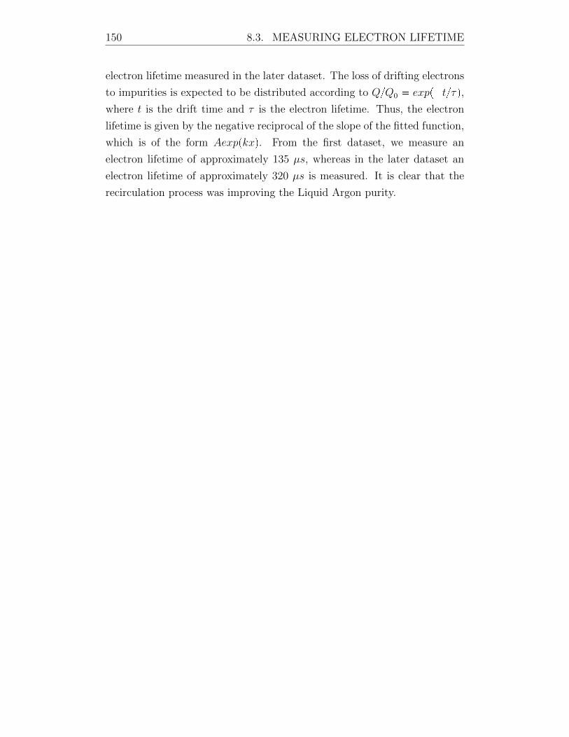
150 8.3. MEASURING ELECTRON LIFETIME
electron lifetime measured in the later dataset. The loss of drifting electrons
to impurities is expected to be distributed according to QQ0 expptτq,where t is the drift time and τ is the electron lifetime. Thus, the electron
lifetime is given by the negative reciprocal of the slope of the fitted function,
which is of the form Aexppkxq. From the first dataset, we measure an
electron lifetime of approximately 135 µs, whereas in the later dataset an
electron lifetime of approximately 320 µs is measured. It is clear that the
recirculation process was improving the Liquid Argon purity.
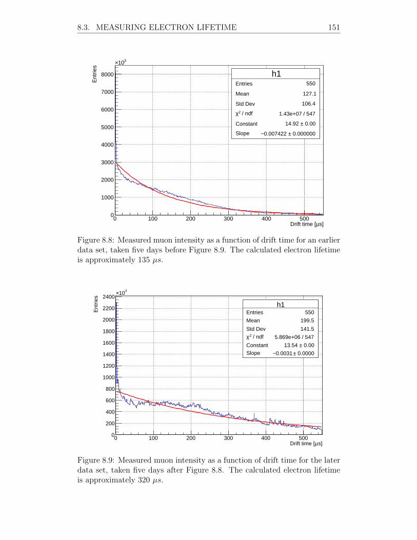
8.3. MEASURING ELECTRON LIFETIME 151
h1Entries 550
Mean 127.1
Std Dev 106.4
/ ndf 2χ 1.43e+07 / 547
Constant 0.00± 14.92
Slope 0.000000±0.007422 −
0 100 200 300 400 500s]µDrift time [
0
1000
2000
3000
4000
5000
6000
7000
8000
310×
Ent
ries
h1Entries 550
Mean 127.1
Std Dev 106.4
/ ndf 2χ 1.43e+07 / 547
Constant 0.00± 14.92
Slope 0.000000±0.007422 −
Figure 8.8: Measured muon intensity as a function of drift time for an earlierdata set, taken five days before Figure 8.9. The calculated electron lifetimeis approximately 135 µs.
h1Entries 550
Mean 199.5
Std Dev 141.5 / ndf 2χ 5.869e+06 / 547
Constant 0.00± 13.54 Slope 0.0000±0.0031 −
0 100 200 300 400 500s]µDrift time [
0
200
400
600
800
1000
1200
1400
1600
1800
2000
2200
2400310×
Ent
ries
h1Entries 550
Mean 199.5
Std Dev 141.5 / ndf 2χ 5.869e+06 / 547
Constant 0.00± 13.54 Slope 0.0000±0.0031 −
Figure 8.9: Measured muon intensity as a function of drift time for the laterdata set, taken five days after Figure 8.8. The calculated electron lifetimeis approximately 320 µs.
152 8.4. ENERGY DEPOSITION OF THROUGHGOING MIPS
8.4 Energy deposition of throughgoing MIPs
The energy loss of throughgoing MIPs can be measured in several ways. Typ-
ical methods involve measuring the mean energy loss and the most probable
energy loss. The distribution formed from taking a sample of the energy loss
along many single segments of a minimum ionising track should generally be
distributed according to a Landau distribution. From this distribution we
could measure two quantities. First, we could measure the mean energy loss,
below a certain cutoff energy. Or, we could fit a Landau function to the dis-
tribution and measure the most probable value (MPV) of this distribution.
Both methods have their own merits and caveats, but here we will focus
on the later technique. The MPV energy loss for highly energetic muons is
approximately 1.6 MeV/cm [121]. Using a short (1 hour) sample of cosmic
data in ARIADNE, we can measure the energy deposition of throughgoing
cosmic muons. For this analysis, event selection is as follows;
1. Raw data is composed of both hits from TPX3Cam and trigger times-
tamp signals from the PMT. Trigger timestamp signals are assumed
to correspond to S1 (t0).
2. For each PMT trigger timestamp t0, collect all hits between t0 and
t0 550 µs (maximum ARIADNE drift length). Hits with ToT 20
ADU are cut.
3. Cut those events which contain less than 1000 hits. This cut broadly
selects track-like events.
4. A purity correction of τ 320 µs is applied to the data. This is done
by adjusting the ToT value of hits according to their drift length by
QQ0 expptτq where Q is the measured ToT value, Q0 is the
corrected ToT value, t is the drift time and τ is the electron lifetime.
5. Perform a robust linear fit 2 in both x-z and y-z planes. The R-Squared
value must be ¡ 0.8 in both planes. Combine these two 2D linear fits
to determine the 3D entry/exit points of the track in the TPC.
6. Cut hits that are further than 20mm from the fitted 3D line.
2https://www.gnu.org/software/gsl/doc/html/lls.html#
robust-linear-regression
8.4. ENERGY DEPOSITION OF THROUGHGOING MIPS 153
7. For all remaining hits, find the closest point on the fitted line to the
hit.
8. Calculate the distance from the track starting point to the closest point
on the fitted line.
9. Fill a histogram bin with the ToT value of this hit. The bin number
to be filled is the distance from the start of the track to the calculated
closest point on the fitted line. The resulting histogram is a histogram
of energy deposition as a function of track length.
10. Taking each bin of the previous histogram, plot a histogram of energy
deposition per 1 mm step in track length. This is a histogram of energy
deposition per 1 mm step size in the TPC, and should be distributed
according to a Landau distribution for a MIP.
Figures 8.10 and 8.11 show two sample distributions from the data set,
with the associated Landau fit.
By taking the mean MPV values for these fitted distributions across
the dataset, we are able to build an energy calibration. Figure 8.12 shows
the average MPV from well fitted tracks. By using the previously found
x dEdXy
MPVof 1.6 MeV/cm through a 1 mm thickness of Liquid Argon, we
can approximate a very coarse energy calibration of 3470 680 ADU/MeV.
A slice width of 1 mm was chosen to maximise the number of available
entries for fitting MPV distributions, examples of which are seen in Figures
8.10 and 8.11. The slice width of 1 mm takes maximal advantage of the
1 mm/pixel tracking resolution in the detector. This calibration will easily
be improved in future work, using longer datasets with improved electron
lifetime.
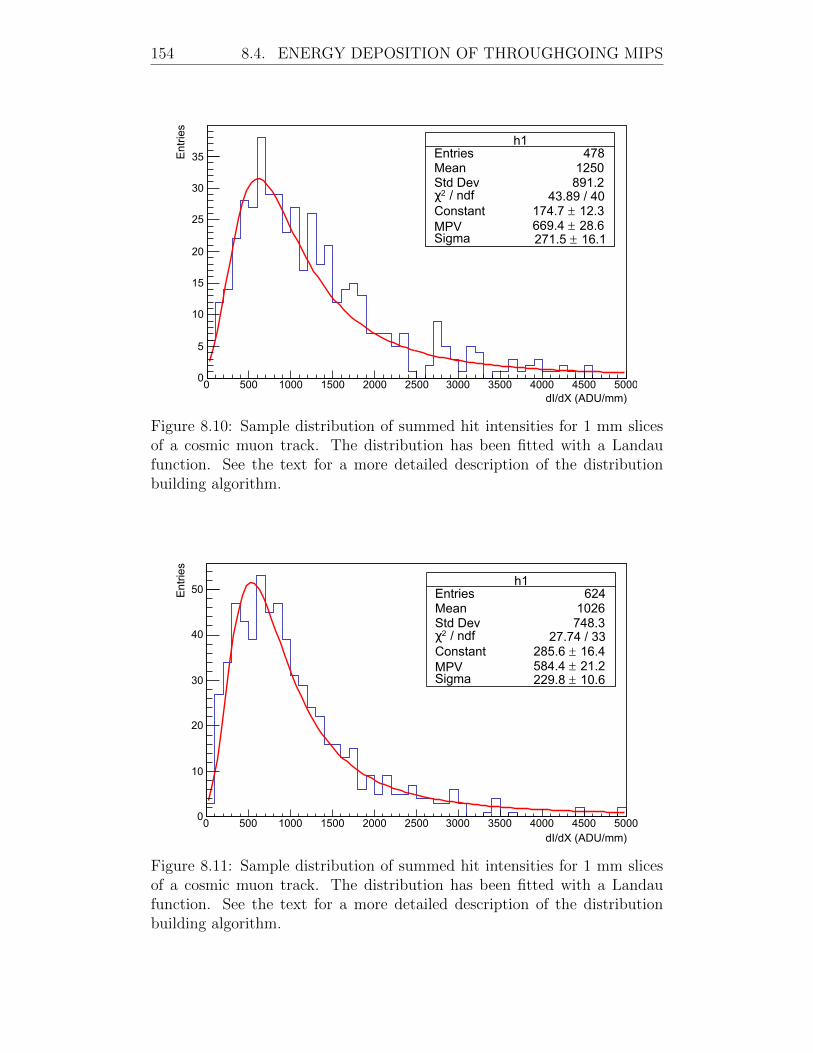
154 8.4. ENERGY DEPOSITION OF THROUGHGOING MIPS
h1Entries 478Mean 1250Std Dev 891.2
/ ndf 2χ 43.89 / 40Constant 12.3174.7 MPV 28.6669.4 Sigma 16.1271.5
0 500 1000 1500 2000 2500 3000 3500 4000 4500 50000
5
10
15
20
25
30
35
h1Entries 478Mean 1250Std Dev 891.2
/ ndf 2χ 43.89 / 40Constant 12.3174.7 MPV 28.6669.4 Sigma 16.1271.5
dI/dX (ADU/mm)
DU/mm)E
ntrie
s
Figure 8.10: Sample distribution of summed hit intensities for 1 mm slicesof a cosmic muon track. The distribution has been fitted with a Landaufunction. See the text for a more detailed description of the distributionbuilding algorithm.
h1Entries 624Mean 1026Std Dev 748.3
/ ndf 2χ 27.74 / 33Constant 16.4285.6 MPV 21.2584.4 Sigma 10.6229.8
0 500 1000 1500 2000 2500 3000 3500 4000 4500 50000
10
20
30
40
50h1
Entries 624Mean 1026Std Dev 748.3
/ ndf 2χ 27.74 / 33Constant 16.4285.6 MPV 21.2584.4 Sigma 10.6229.8
Ent
ries
dI/dX (ADU/mm)
Figure 8.11: Sample distribution of summed hit intensities for 1 mm slicesof a cosmic muon track. The distribution has been fitted with a Landaufunction. See the text for a more detailed description of the distributionbuilding algorithm.
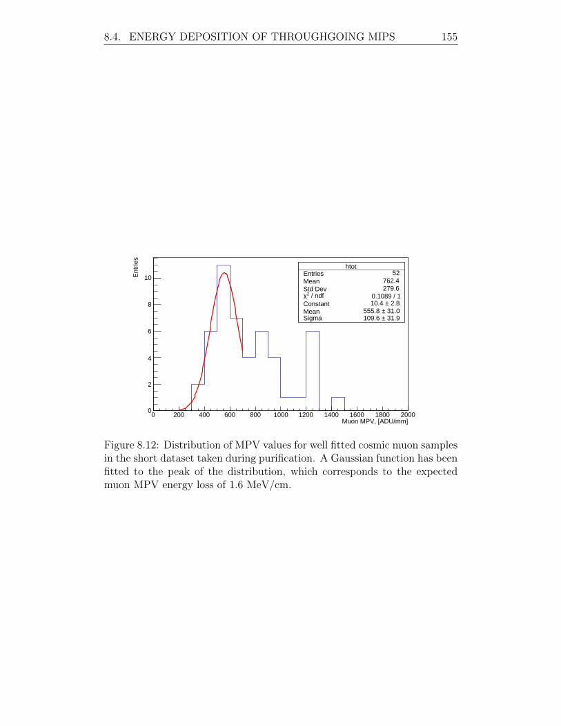
8.4. ENERGY DEPOSITION OF THROUGHGOING MIPS 155
htotEntries 52Mean 762.4Std Dev 279.6
/ ndf 2χ 0.1089 / 1Constant 2.8± 10.4 Mean 31.0± 555.8 Sigma 31.9± 109.6
0 200 400 600 800 1000 1200 1400 1600 1800 2000Muon MPV, [ADU/mm]
0
2
4
6
8
10Ent
ries
htotEntries 52Mean 762.4Std Dev 279.6
/ ndf 2χ 0.1089 / 1Constant 2.8± 10.4 Mean 31.0± 555.8 Sigma 31.9± 109.6
Figure 8.12: Distribution of MPV values for well fitted cosmic muon samplesin the short dataset taken during purification. A Gaussian function has beenfitted to the peak of the distribution, which corresponds to the expectedmuon MPV energy loss of 1.6 MeV/cm.
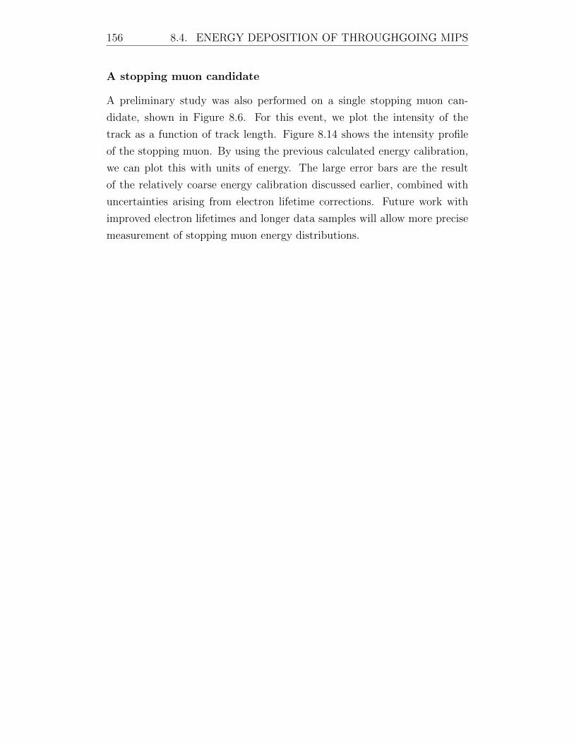
156 8.4. ENERGY DEPOSITION OF THROUGHGOING MIPS
A stopping muon candidate
A preliminary study was also performed on a single stopping muon can-
didate, shown in Figure 8.6. For this event, we plot the intensity of the
track as a function of track length. Figure 8.14 shows the intensity profile
of the stopping muon. By using the previous calculated energy calibration,
we can plot this with units of energy. The large error bars are the result
of the relatively coarse energy calibration discussed earlier, combined with
uncertainties arising from electron lifetime corrections. Future work with
improved electron lifetimes and longer data samples will allow more precise
measurement of stopping muon energy distributions.
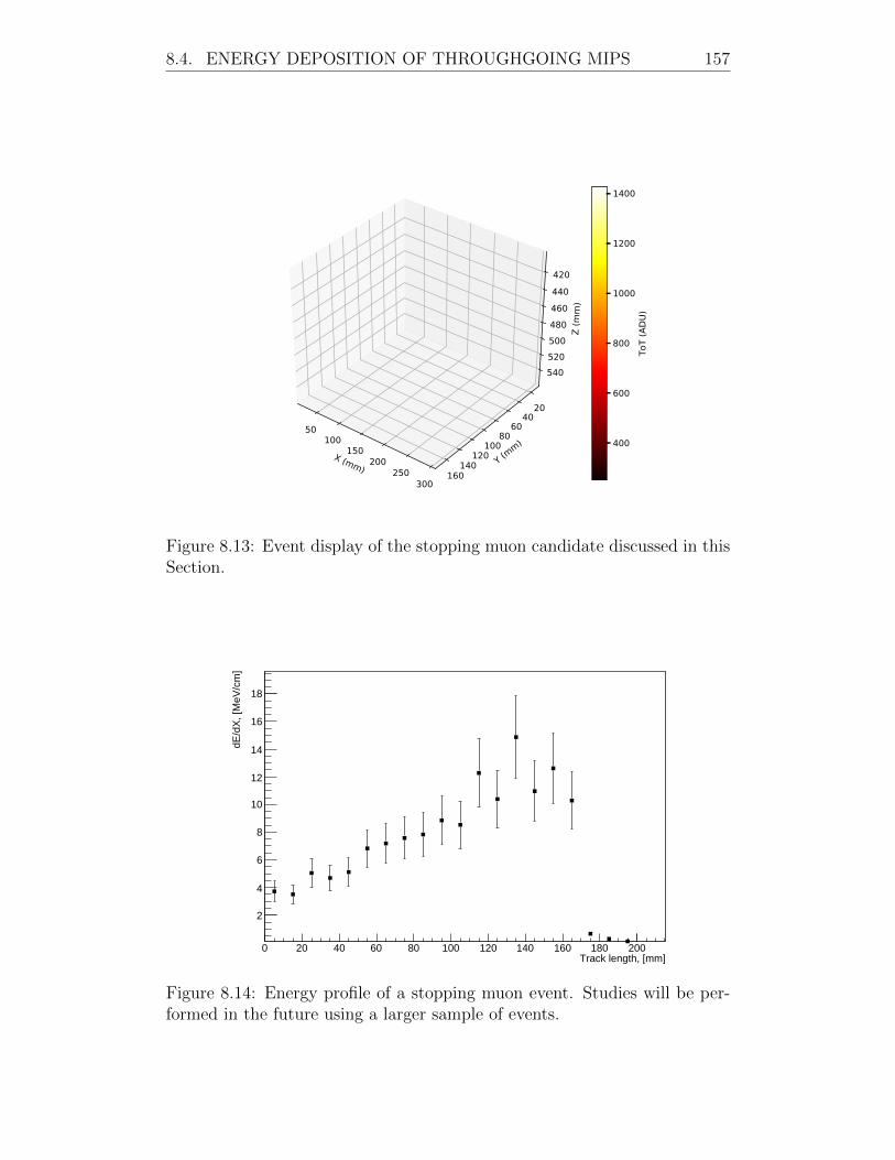
8.4. ENERGY DEPOSITION OF THROUGHGOING MIPS 157
X (mm)
50100
150200
250300
Y (mm)
2040
6080
100120
140160
Z (m
m)
420440460480500520540
400
600
800
1000
1200
1400
ToT
(ADU
)
Figure 8.13: Event display of the stopping muon candidate discussed in thisSection.
0 20 40 60 80 100 120 140 160 180 200Track length, [mm]
2
4
6
8
10
12
14
16
18
dE/d
X, [
MeV
/cm
]
Figure 8.14: Energy profile of a stopping muon event. Studies will be per-formed in the future using a larger sample of events.
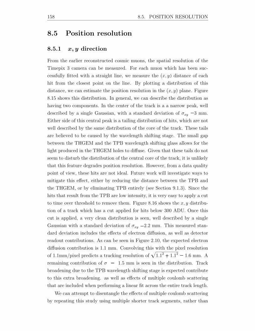
158 8.5. POSITION RESOLUTION
8.5 Position resolution
8.5.1 x, y direction
From the earlier reconstructed cosmic muons, the spatial resolution of the
Timepix 3 camera can be measured. For each muon which has been suc-
cessfully fitted with a straight line, we measure the px, yq distance of each
hit from the closest point on the line. By plotting a distribution of this
distance, we can estimate the position resolution in the px, yq plane. Figure
8.15 shows this distribution. In general, we can describe the distribution as
having two components. In the center of the track is a a narrow peak, well
described by a single Gaussian, with a standard deviation of σxy 3 mm.
Either side of this central peak is a tailing distribution of hits, which are not
well described by the same distribution of the core of the track. These tails
are believed to be caused by the wavelength shifting stage. The small gap
between the THGEM and the TPB wavelength shifting glass allows for the
light produced in the THGEM holes to diffuse. Given that these tails do not
seem to disturb the distribution of the central core of the track, it is unlikely
that this feature degrades position resolution. However, from a data quality
point of view, these hits are not ideal. Future work will investigate ways to
mitigate this effect, either by reducing the distance between the TPB and
the THGEM, or by eliminating TPB entirely (see Section 9.1.3). Since the
hits that result from the TPB are low intensity, it is very easy to apply a cut
to time over threshold to remove them. Figure 8.16 shows the x, y distribu-
tion of a track which has a cut applied for hits below 300 ADU. Once this
cut is applied, a very clean distribution is seen, well described by a single
Gaussian with a standard deviation of σxy 2.2 mm. This measured stan-
dard deviation includes the effects of electron diffusion, as well as detector
readout contributions. As can be seen in Figure 2.10, the expected electron
diffusion contribution is 1.1 mm. Convolving this with the pixel resolution
of 1.1mm/pixel predicts a tracking resolution ofa
1.12 1.12 1.6 mm. A
remaining contribution of σ 1.5 mm is seen in the distribution. Track
broadening due to the TPB wavelength shifting stage is expected contribute
to this extra broadening. as well as effects of multiple coulomb scattering
that are included when performing a linear fit across the entire track length.
We can attempt to disentangle the effects of multiple coulomb scattering
by repeating this study using multiple shorter track segments, rather than
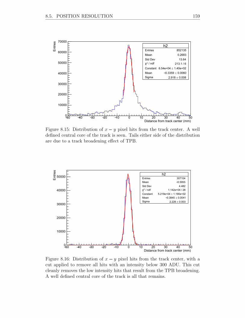
8.5. POSITION RESOLUTION 159
h2Entries 852135
Mean 0.2683
Std Dev 13.64
/ ndf 2χ 213.1 / 6
Constant 1.40e+026.54e+04
Mean 0.00600.3359 −
Sigma 0.0082.918
50− 40− 30− 20− 10− 0 10 20 30 40 500
10000
20000
30000
40000
50000
60000
70000
h2Entries 852135
Mean 0.2683
Std Dev 13.64
/ ndf 2χ 213.1 / 6
Constant 1.40e+026.54e+04
Mean 0.00600.3359 −
Sigma 0.0082.918
Ent
ries
Distance from track center (mm)
Figure 8.15: Distribution of x y pixel hits from the track center. A welldefined central core of the track is seen. Tails either side of the distributionare due to a track broadening effect of TPB.
h2Entries 307104
Mean 0.5955−
Std Dev 4.482
/ ndf 2χ 1.142e+04 / 28
Constant 1.190e+025.219e+04
Mean 0.00410.3845 −Sigma 0.0032.226
50− 40− 30− 20− 10− 0 10 20 30 40 500
10000
20000
30000
40000
50000h2
Entries 307104
Mean 0.5955−
Std Dev 4.482
/ ndf 2χ 1.142e+04 / 28
Constant 1.190e+025.219e+04
Mean 0.00410.3845 −Sigma 0.0032.226
Distance from track center (mm)
Ent
ries
Figure 8.16: Distribution of x y pixel hits from the track center, with acut applied to remove all hits with an intensity below 300 ADU. This cutcleanly removes the low intensity hits that result from the TPB broadening.A well defined central core of the track is all that remains.
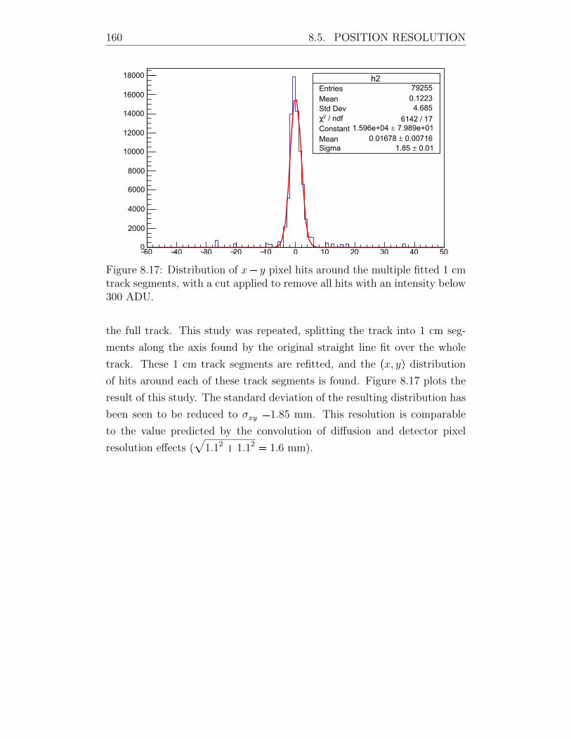
160 8.5. POSITION RESOLUTION
h2Entries 79255
Mean 0.1223Std Dev 4.685
/ ndf 2χ 6142 / 17Constant 7.989e+011.596e+04
Mean 0.007160.01678 Sigma 0.011.85
50− 40− 30− 20− 10− 0 10 20 30 40 500
2000
4000
6000
8000
10000
12000
14000
16000
18000 h2Entries 79255
Mean 0.1223Std Dev 4.685
/ ndf 2χ 6142 / 17Constant 7.989e+011.596e+04
Mean 0.007160.01678 Sigma 0.011.85
Figure 8.17: Distribution of x y pixel hits around the multiple fitted 1 cmtrack segments, with a cut applied to remove all hits with an intensity below300 ADU.
the full track. This study was repeated, splitting the track into 1 cm seg-
ments along the axis found by the original straight line fit over the whole
track. These 1 cm track segments are refitted, and the px, yq distribution
of hits around each of these track segments is found. Figure 8.17 plots the
result of this study. The standard deviation of the resulting distribution has
been seen to be reduced to σxy 1.85 mm. This resolution is comparable
to the value predicted by the convolution of diffusion and detector pixel
resolution effects (a
1.12 1.12 1.6 mm).
8.6. DISCUSSION 161
8.5.2 z direction
In the z direction, we will discuss the resolution in units of time. For clean
throughgoing MIPs, Figures 8.18 and 8.19 present the timing distribution
of hits, relative to the track center. Both are well described by a single
Gaussian, with a standard deviation of approximately 1 µs. These results
can be interpreted in mm using a conversion of 1.648 mm/µs. Applying a
ToT cut to remove the effect of the TPB broadening, as was done in the
x, y plane, does not make any noticeable change to the resolution in the z
axis. This is to be expected, since the TPB broadening effect should only
be a spatial effect in the x, y plane, and not affect timing, which ultimately
dictates the z position resolution. It is worthwhile to note that z position
resolution should not change with varying field of view of the camera. If a
larger detector area is covered per camera, the x, y resolution will be reduced.
However, the z resolution is dictated by the timing resolution of the TPX3
ASIC and should remain excellent.
8.6 Discussion
Performance of the TPX3 based cameras in Liquid Argon was generally
found to be excellent. The timestamping capability of TPX3Cam was found
to provide extremely precise z axis resolution. Now, a single camera is
capable of performing readout of all px, y, z, Eq. When compared to the
EMCCD cameras, TPX3Cam combined with an intensifier seemed to offer
comparable or even greater sensitivity.
Correlation of the camera with a PMT using the external timestamping
signal feature was tested thoroughly. The connection appeared robust, with
no obvious timing problems being seen. The effect of track broadening by
TPB was closely studied. Once suitable cuts are selected, it seems that this
effect had a negligible impact on tracking resolution. In the future, options
will be explored to reduce or even eliminate this TPB component.
At the time of writing, the ARIADNE detector continues to be purified.
Currently, the electron lifetime is in the region of 350 microseconds. Once a
suitable electron lifetime is achieved, perhaps closer to several milliseconds,
more detailed analyses will be performed. Longer datasets will be taken with
improved electron lifetime, providing greater statistics while simultaneously
reducing the magnitude of systematic uncertainties introduced by purity

162 8.6. DISCUSSION
Hit distance from track center (microseconds)
Ent
ries
h2Entries 2005Mean 1.419−Std Dev 1.196
/ ndf 2χ 96.25 / 18Constant 11.9351.2 Mean 0.0251.451 −Sigma 0.0271.084
10− 8− 6− 4− 2− 0 2 4 6 8 100
50
100
150
200
250
300
350
400h2
Entries 2005Mean 1.419−Std Dev 1.196
/ ndf 2χ 96.25 / 18Constant 11.9351.2 Mean 0.0251.451 −Sigma 0.0271.084
Figure 8.18: Distribution of hit timings in the z axis, relative to the centerof the fitted track. The distribution is well described by a Gaussian, with astandard deviation of only 1 microsecond.
h2Entries 3203Mean 1.247−Std Dev 1.236
/ ndf 2χ 79.83 / 24Constant 13.0545.7 Mean 0.0211.279 −Sigma 0.0181.142
10− 8− 6− 4− 2− 0 2 4 6 8 100
100
200
300
400
500
600
h2Entries 3203Mean 1.247−Std Dev 1.236
/ ndf 2χ 79.83 / 24Constant 13.0545.7 Mean 0.0211.279 −Sigma 0.0181.142
Hit distance from track center (microseconds)
Ent
ries
Figure 8.19: Distribution of hit timings in the z axis for a second exampletrack, relative to the center of the fitted track. The distribution is also welldescribed by a Gaussian.

8.6. DISCUSSION 163
corrections. This should allow for a much more robust energy calibration of
the system. It is expected that a more complete sample of stopping muons
will also be obtained, allowing more detailed studies to be performed. The
intensity profile of stopping muons can be analysed in much greater detail,
and perhaps the energy distribution of the resulting Michel electrons can
also be measured.
Chapter 9
Future developments
9.1 Technological advances
Several profitable technological developments may be realised in the near
future. Three flavours of improvements are particularly interesting. Devel-
opments of new versions of the Timepix ASIC should provide compelling cost
reductions and performance improvements. Improvements in image intensi-
fier photocathode quantum efficiency presents the opportunity for improved
light collection. Recent image intensifier advancements have also presented
an intriguing opportunity for potential direct imaging of VUV scintillation
light, without use of a wavelength shifter. Finally, some interesting pos-
sibilities are emerging for THGEM designs which have been tailored for
electroluminescence light production.
9.1.1 Timepix 4
The Medipix4 Collaboration is currently developing the Timepix4 (TPX4)
ASIC [122]. The exact specification of TPX4 is not yet formally defined
although the main design goals are a larger ASIC (close to 512 512 pixels)
and improved resolution of both ToT and ToA. Given that the 1.6 ns timing
resolution of TPX3 was already ample for optical readout of both gas and
liquid TPCs, the improvements to ToA resolution are not especially interest-
ing. The improvement of ToT resolution should enhance calorimetric per-
formance. The improved 12-bit resolution of TPX4 is now only marginally
less than the 14-bit resolution proposed by two-phase charge readout tech-
nologies. The larger size of the TPX4 ASIC means that a larger detector
164
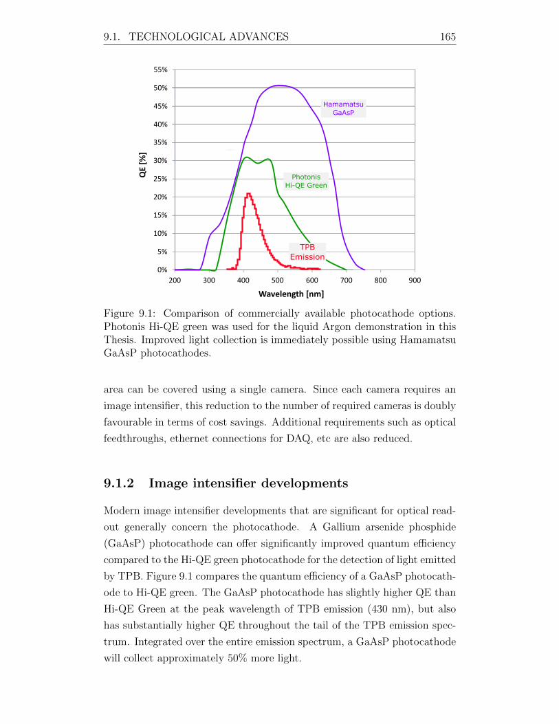
9.1. TECHNOLOGICAL ADVANCES 165
0%
5%
10%
15%
20%
25%
30%
35%
200 300 400 500 600 700 800 900
QE
[%]
Wavelength [nm]
PhotonisHi-QE Green
40%
45%
50%
55%
TPBEmission
HamamatsuGaAsP
Figure 9.1: Comparison of commercially available photocathode options.Photonis Hi-QE green was used for the liquid Argon demonstration in thisThesis. Improved light collection is immediately possible using HamamatsuGaAsP photocathodes.
area can be covered using a single camera. Since each camera requires an
image intensifier, this reduction to the number of required cameras is doubly
favourable in terms of cost savings. Additional requirements such as optical
feedthroughs, ethernet connections for DAQ, etc are also reduced.
9.1.2 Image intensifier developments
Modern image intensifier developments that are significant for optical read-
out generally concern the photocathode. A Gallium arsenide phosphide
(GaAsP) photocathode can offer significantly improved quantum efficiency
compared to the Hi-QE green photocathode for the detection of light emitted
by TPB. Figure 9.1 compares the quantum efficiency of a GaAsP photocath-
ode to Hi-QE green. The GaAsP photocathode has slightly higher QE than
Hi-QE Green at the peak wavelength of TPB emission (430 nm), but also
has substantially higher QE throughout the tail of the TPB emission spec-
trum. Integrated over the entire emission spectrum, a GaAsP photocathode
will collect approximately 50% more light.
166 9.1. TECHNOLOGICAL ADVANCES
9.1.3 Direct VUV imaging
An exciting possibility may result in the elimination of the TPB wavelength
shifter all together. Certain photocathodes exhibit good quantum efficiency
in the VUV, making direct detection of the VUV scintillation light from
Argon (or Xenon) a possibility. Although TPB is frequently used, it is not
without problems. The coating process requires careful consideration to en-
sure that the coating has both a well defined thickness that this thickness
is uniform over the whole surface. It is conceivable that variations in TPB
coating thickness would induce variations in detector response. Addition-
ally, TPB coatings have been shown to degrade under UV exposure [123].
Losses can be as high as 40 % with a single day of exposure to ambient
light. Considerations to protect TPB coatings from ambient light can result
in added expense and complication. TPB has been shown to have a clear
aging effect when exposed to ambient light [124]. Beyond these initial man-
ufacturing concerns, TPB may also result in subtle yet important changes
to detector performance. Considering its widespread application, the emis-
sion time spectrum of TPB has not been studied in much detail. Recent
studies have discovered the existence of a long lived triplet states in TPB
[125]. The existence of these states has been suggested as an explanation for
often observed ’intermediate’ decay components, which have no basis in the
known emission spectrum of pure Argon. This highlights the care that must
be taken when introducing an additional step in a detection process. Unless
a complete and thorough understanding of the process is known, subtleties
can present themselves. Given this, perhaps the elimination of the TPB
wavelength shifting step is pragmatic.
Direct VUV optical readout requires both an image intensifier that is
sensitive to 128nm as well as suitable optics. Cesium iodode (CsI) coated
MCPs have historically been produced with quantum efficiencies generally in
the region of 20 % to 30 % [126–131]. The performance of CsI photocathodes
has been found to be stable over at least six years of operation [132]. Photek
Limited, a manufacturer of image intensifiers based in the UK, has recently
developed CsI coated MCPs with detection efficiencies in the range of 20 %
to 35 % at 128 nm, measured behind a magnesium fluoride input window.
In order to be transparent to 128 nm photons, an intensifier should use
an input window made from Magnesium Fluoride (MgF2). The transmission
of MgF2 at 128 nm is around 65 %, and close to 90 % at 178 nm.
9.1. TECHNOLOGICAL ADVANCES 167
An MgF2 imaging lens is required on the detector side, focusing the
VUV photons onto the input window of the intensifier. This lens should
have around 65 % transparency at 128 nm, reducing detection efficiency
from 20-35 % to 13-23 %. Although this detection efficiency, at first glace,
seems inferior to the roughly 30 % DQE currently achieved with Hi-QE
green photocathode, the elimination of the TPB wavelength shifting step
should realise substantial improvements in light collection efficiency. We
can express the total light collection efficiency of the optical readout setup
as
η ηWLSΩλDQE (9.1)
where ηWLS represents the efficiency of the wavelength shifting process, Ω
represents the solid angle from the TPB to the lens and λDQE represents the
detective efficiency of readout device (either optical or VUV). Given that
the solid angle is the same for both optical or VUV readout, we can express
the relative detection efficiency between the two approaches as
ηVUV
ηOptical
λVUV
ηWLSλOptical
(9.2)
We know that λOptical is 30% for the Photonis cricket and we will assume
λVUV of 18%, based from the average of photocathodes that were produced
by Photek, discussed earlier. Thus,
ηVUV
ηOptical
0.6
ηWLS
(9.3)
Thus, ηVUV is greater than ηOptical for any ηWLS less than 60%. Even if we
assume that all light production happens at the top of the THGEM hole,
and that any light produced that hits the TPB is converted to useful light,
ηWLS reaches a theoretical maximum of 50%, given that half of the light
produced in any hole goes downwards, away from the TPB. Thus, direct
VUV imaging seems promising for improved detection efficiency.
In reality, ηWLS is not going to be 50%. A more realistic value may be
predicted by assuming all light production happens in the middle of the hole
thickness, which yields ηWLS of only 6%.
Separating the imaging lens and intensifier input window allows some
flexibility for lens R&D. Different lenses can be exchanged without disturb-
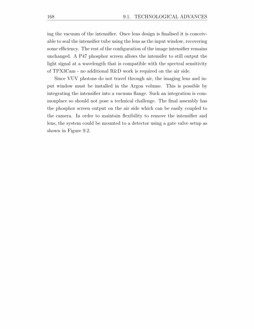
168 9.1. TECHNOLOGICAL ADVANCES
ing the vacuum of the intensifier. Once lens design is finalised it is conceiv-
able to seal the intensifier tube using the lens as the input window, recovering
some efficiency. The rest of the configuration of the image intensifier remains
unchanged. A P47 phosphor screen allows the intensifer to still output the
light signal at a wavelength that is compatible with the spectral sensitivity
of TPX3Cam - no additional R&D work is required on the air side.
Since VUV photons do not travel through air, the imaging lens and in-
put window must be installed in the Argon volume. This is possible by
integrating the intensifier into a vacuum flange. Such an integration is com-
monplace so should not pose a technical challenge. The final assembly has
the phosphor screen output on the air side which can be easily coupled to
the camera. In order to maintain flexibility to remove the intensifier and
lens, the system could be mounted to a detector using a gate valve setup as
shown in Figure 9.2.
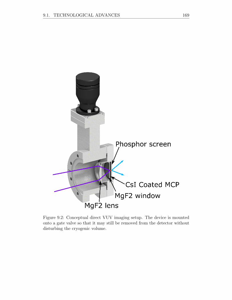
9.1. TECHNOLOGICAL ADVANCES 169
Figure 9.2: Conceptual direct VUV imaging setup. The device is mountedonto a gate valve so that it may still be removed from the detector withoutdisturbing the cryogenic volume.
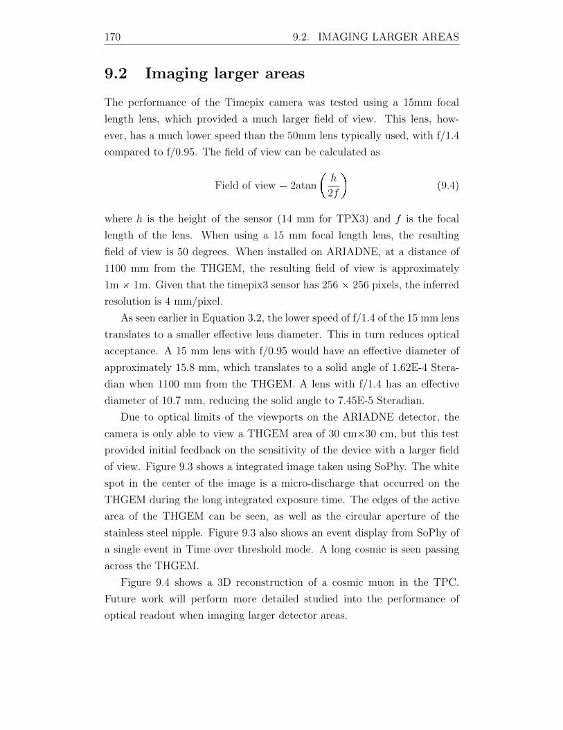
170 9.2. IMAGING LARGER AREAS
9.2 Imaging larger areas
The performance of the Timepix camera was tested using a 15mm focal
length lens, which provided a much larger field of view. This lens, how-
ever, has a much lower speed than the 50mm lens typically used, with f/1.4
compared to f/0.95. The field of view can be calculated as
Field of view 2atan
h
2f
(9.4)
where h is the height of the sensor (14 mm for TPX3) and f is the focal
length of the lens. When using a 15 mm focal length lens, the resulting
field of view is 50 degrees. When installed on ARIADNE, at a distance of
1100 mm from the THGEM, the resulting field of view is approximately
1m 1m. Given that the timepix3 sensor has 256 256 pixels, the inferred
resolution is 4 mm/pixel.
As seen earlier in Equation 3.2, the lower speed of f/1.4 of the 15 mm lens
translates to a smaller effective lens diameter. This in turn reduces optical
acceptance. A 15 mm lens with f/0.95 would have an effective diameter of
approximately 15.8 mm, which translates to a solid angle of 1.62E-4 Stera-
dian when 1100 mm from the THGEM. A lens with f/1.4 has an effective
diameter of 10.7 mm, reducing the solid angle to 7.45E-5 Steradian.
Due to optical limits of the viewports on the ARIADNE detector, the
camera is only able to view a THGEM area of 30 cm30 cm, but this test
provided initial feedback on the sensitivity of the device with a larger field
of view. Figure 9.3 shows a integrated image taken using SoPhy. The white
spot in the center of the image is a micro-discharge that occurred on the
THGEM during the long integrated exposure time. The edges of the active
area of the THGEM can be seen, as well as the circular aperture of the
stainless steel nipple. Figure 9.3 also shows an event display from SoPhy of
a single event in Time over threshold mode. A long cosmic is seen passing
across the THGEM.
Figure 9.4 shows a 3D reconstruction of a cosmic muon in the TPC.
Future work will perform more detailed studied into the performance of
optical readout when imaging larger detector areas.
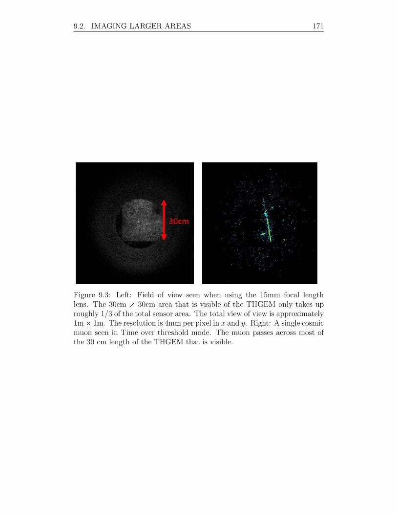
9.2. IMAGING LARGER AREAS 171
Figure 9.3: Left: Field of view seen when using the 15mm focal lengthlens. The 30cm 30cm area that is visible of the THGEM only takes uproughly 1/3 of the total sensor area. The total view of view is approximately1m 1m. The resolution is 4mm per pixel in x and y. Right: A single cosmicmuon seen in Time over threshold mode. The muon passes across most ofthe 30 cm length of the THGEM that is visible.
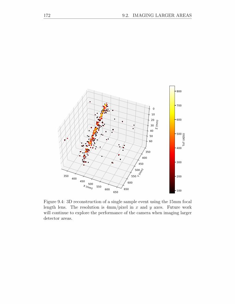
172 9.2. IMAGING LARGER AREAS
X (mm)
350400
450500
550600
650
Y (mm)
350
400
450
500
550
600
650
Z (m
m)
0
10
20
30405060
100
200
300
400
500
600
700
800
ToT
(ADU
)
Figure 9.4: 3D reconstruction of a single sample event using the 15mm focallength lens. The resolution is 4mm/pixel in x and y axes. Future workwill continue to explore the performance of the camera when imaging largerdetector areas.
Chapter 10
Conclusion
In Chapter 1, the current state of neutrino physics is briefly discussed, pro-
viding a motivation for the construction and use of Liquid Argon TPCs as a
tool for future discoveries. In Chapter 2, the operation aspects of dual-phase
Liquid Argon TPCs are discussed in detail.
In Chapter 3, the concept of optical readout of a dual-phase Liquid Argon
TPC is introduced. A model of THGEM light production is presented.
The rate of light production in a THGEM is compared to that of charge
production.
Chapter 4 introduces the ARIADNE detector. The ARIADNE detector
is discussed from design phase, through to construction and finally opera-
tion ongoing at the time of writing. Key design aspects are explained in
detail and possible future improvements are also discussed. The design and
manufacture of the ARIADNE 100 kV high voltage feedthrough is explained.
In Chapter 5, the deployment of the ARIADNE detector to the CERN
T9 beamline is presented. Results from beamline operation highlighted the
excellent sensitivity of EMCCD cameras, as well as excellent x, y resolution.
Subsequent analysis of the data taken at the beamline showed that z di-
mension reconstruction using EMCCDs can be challenging. This limitation
motivated R&D activities, culminating in the development of a novel camera
technology. This new camera technology was introduced and characterised
in Chapters 6, 7 and 8. Full px, y, z, Eq readout is now possible using a single
device.
Many benefits were found during testing;
• Externally mounted cameras provided easy access for upgrade, repair
and calibration throughout the life of an experiment.
173
174
• Sensitivity to the linear electroluminescence light produced by the
THGEM was demonstrated. Operation of the THGEM at low field
may help to ease problems related to ion backflow.
• Millimeter scale resolution in x, y and z axes was demonstrated.
• The zero-suppressed and natively 3D data format allows for simple
data manipulation during analysis. 3D reconstruction of events is triv-
ial. In Chapter 7, the readout of a gas TPC with a high event rate
(1 kHz) was demonstrated. This demonstrates the flexibility of the
technology for applications beyond dual-phase Liquid Argon TPCs.
Future developments are certain to continue to improve the performance
of optical readout. In particular, development of direct VUV imaging tech-
nologies are particularly exciting, discussed in Section 9.1.3. In future work,
the potential application of optical readout in the context of future kiloton
scale LArTPCs will be explored. In Section 9.2, we saw that preliminary
testing using a 1m 1m field of view, on initial impressions, seems to retain
good sensitivity.
In the future, the Timepix 4 ASIC with its larger sensor size may allow
the readout of increased readout areas, closer to 1.5m 1.5m per camera.
Future work will investigate the applicability of optical readout to larger
detector areas. Considering the proposed 720 m2 readout area per DUNE
module, a 1.5m 1.5m field of view per camera could allow detector readout
using only 320 cameras with 2-3 millimeter scale resolution in all axes.
Bibliography
[1] DUNE Collaboration et al. “Long-Baseline Neutrino Facility (LBNF)
and Deep Underground Neutrino Experiment (DUNE) Conceptual
Design Report Volume 2: The Physics Program for DUNE at LBNF”.
In: 2 (Dec. 2015). arXiv: 1512.06148. url: http://arxiv.org/abs/
1512.06148.
[2] Adam Roberts et al. “ARIADNE, a Photographic Two-Phase LAr
TPC”. In: Proceedings of The European Physical Society Conference
on High Energy Physics — PoS(EPS-HEP2017). Trieste, Italy: Sissa
Medialab, Jan. 2018, p. 802. doi: 10.22323/1.314.0802. url:
https://pos.sissa.it/314/802.
[3] Simeon Bird et al. “Did LIGO Detect Dark Matter?” In: Physical
Review Letters 116.20 (May 2016), p. 201301. issn: 0031-9007. doi:
10.1103/PhysRevLett.116.201301. arXiv: arXiv:1603.00464v2.
url: https://link.aps.org/doi/10.1103/PhysRevLett.116.
201301.
[4] Carlo Giunti and Chung W. Kim. Fundamentals of Neutrino Physics
and Astrophysics. Oxford University Press, Mar. 2007. isbn: 9780198508717.
doi: 10.1093/acprof:oso/9780198508717.001.0001. url: http:
//www.oxfordscholarship.com/view/10.1093/acprof:oso/
9780198508717.001.0001/acprof-9780198508717.
[5] M. Tanabashi et al. “Review of Particle Physics”. In: Physical Review
D 98.3 (2018), p. 30001. issn: 24700029. doi: 10.1103/PhysRevD.
98.030001. url: https://doi.org/10.1103/PhysRevD.98.030001.
[6] F. P. An et al. “Search for a Light Sterile Neutrino at Daya Bay”.
In: Journal of Physics: Conference Series 888.1 (July 2014), pp. 1–7.
issn: 17426596. doi: 10.1103/PhysRevLett.113.141802. arXiv:
175
176 BIBLIOGRAPHY
1407.7259. url: http://arxiv.org/abs/1407.7259%20http:
//dx.doi.org/10.1103/PhysRevLett.113.141802.
[7] M. A. Acero. “Measurement of the neutrino oscillation parameters
by NOvA”. In: Journal of Physics: Conference Series 1219.1 (May
2019), p. 012021. issn: 1742-6588. doi: 10.1088/1742-6596/1219/
1/012021. url: https://iopscience.iop.org/article/10.1088/
1742-6596/1219/1/012021.
[8] K. Abe et al. “Measurement of neutrino and antineutrino oscilla-
tions by the T2K experiment including a new additional sample of
nu e interactions at the far detector”. In: Physical Review D 96.9
(July 2017), pp. 1–50. issn: 24700029. doi: 10.1103/PhysRevD.96.
092006. arXiv: 1707.01048. url: http://dx.doi.org/10.1103/
PhysRevD.96.092006.
[9] K. Abe et al. “Updated T2K measurements of muon neutrino and an-
tineutrino disappearance using 1.5e21 protons on target”. In: Physical
Review D 96.1 (Apr. 2017), pp. 1–8. issn: 24700029. doi: 10.1103/
PhysRevD.96.011102. arXiv: 1704.06409. url: http://dx.doi.
org/10.1103/PhysRevD.96.011102.
[10] Super-Kamiokande Collaboration et al. “Atmospheric Neutrino Os-
cillation Analysis With Improved Event Reconstruction in Super-
Kamiokande IV”. In: Progress of Theoretical and Experimental Physics
2019.5 (Jan. 2019), pp. 1–42. issn: 20503911. doi: 10.1093/ptep/
ptz015. arXiv: 1901.03230. url: http://dx.doi.org/10.1093/
ptep/ptz015.
[11] Paul Langacker. “Grand unified theories and proton decay”. In: Physics
Reports 72.4 (June 1981), pp. 185–385. issn: 03701573. doi: 10 .
1016/0370-1573(81)90059-4. url: https://linkinghub.elsevie
r.com/retrieve/pii/0370157381900594.
[12] Goran Senjanovic. “Proton decay and grand unification”. In: AIP
Conference Proceedings 1200 (Dec. 2009), pp. 131–141. issn: 0094243X.
doi: 10.1063/1.3327552. arXiv: 0912.5375. url: http://dx.doi.
org/10.1063/1.3327552.
BIBLIOGRAPHY 177
[13] The Super-Kamiokande Collaboration et al. “Search for Proton De-
cay into Muon plus Neutral Kaon in Super-Kamiokande I, II, and
III”. In: (May 2012), pp. 1–15. doi: 10.1103/PhysRevD.86.012006.
arXiv: 1205.6538. url: http://dx.doi.org/10.1103/PhysRevD.
86.012006.
[14] The Super-Kamiokande Collaboration et al. “Search for Proton De-
cay via p nu K+ using 260 kiloton year data of Super-Kamiokande”.
In: Physical Review D 90.7 (Aug. 2014), p. 072005. issn: 1550-7998.
doi: 10 . 1103 / PhysRevD . 90 . 072005. arXiv: 1408 . 1195. url:
https://link.aps.org/doi/10.1103/PhysRevD.90.072005.
[15] V. Alan Kostelecky and Matthew Mewes. “Neutrinos with Lorentz-
violating operators of arbitrary dimension”. In: Physical Review D
- Particles, Fields, Gravitation and Cosmology 85.9 (2012), pp. 1–
35. issn: 15507998. doi: 10.1103/PhysRevD.85.096005. arXiv:
1112.6395.
[16] C. E. Aalseth et al. “DarkSide-20k: A 20 tonne two-phase LAr TPC
for direct dark matter detection at LNGS”. In: European Physical
Journal Plus 133.3 (2018). issn: 21905444. doi: 10.1140/epjp/
i2018-11973-4. arXiv: arXiv:1707.08145v1.
[17] J. Calvo et al. “Commissioning of the ArDM experiment at the Can-
franc underground laboratory: first steps towards a tonne-scale liq-
uid argon time projection chamber for Dark Matter searches”. In:
Journal of Cosmology and Astroparticle Physics 2017.03 (Mar. 2017),
pp. 003–003. issn: 1475-7516. doi: 10.1088/1475-7516/2017/03/
003. url: http://stacks.iop.org/1475-7516/2017/i=03/a=003?
key=crossref.866228893f85dbc8e67d1c4d8c018448.
[18] Andre Rubbia. “ArDM: a ton-scale liquid Argon experiment for direct
detection of Dark Matter in the Universe”. In: Journal of Physics:
Conference Series 39.1 (May 2006), pp. 129–132. issn: 1742-6588.
doi: 10.1088/1742-6596/39/1/028. url: http://stacks.iop.
org/1742-6596/39/i=1/a=028?key=crossref.dd9b7c9c6dae25c
6813dd731d3cb135c.
[19] A. Marchionni et al. “ArDM: A ton-scale LAr detector for direct Dark
Matter searches”. In: Journal of Physics: Conference Series 308.1
(2011). issn: 17426596. doi: 10.1088/1742-6596/308/1/012006.
178 BIBLIOGRAPHY
[20] R. Acciarri et al. “The WArP Experiment”. In: Journal of Physics:
Conference Series 308.1 (2011). issn: 17426596. doi: 10.1088/1742-
6596/308/1/012005.
[21] C. Amsler. “Search for WIMPs in liquid argon”. In: (May 2011),
p. 13. arXiv: 1105.4524. url: http://arxiv.org/abs/1105.4524.
[22] Marc Schumann. “Dark Matter Search with liquid Noble Gases”. In:
(June 2012). arXiv: 1206.2169. url: http://arxiv.org/abs/1206.
2169.
[23] B. J. Mount et al. “LUX-ZEPLIN (LZ) Technical Design Report”.
In: (Mar. 2017). arXiv: 1703.09144. url: http://arxiv.org/abs/
1703.09144.
[24] C. Rubbia. “The Liquid Argon Time Projection Chamber: A New
Concept for Neutrino Detectors”. In: CERN-EP/77-08 (1977).
[25] T. Heindl et al. “Table-top setup for investigating the scintillation
properties of liquid argon”. In: Journal of Instrumentation 6.02 (Feb.
2011), P02011–P02011. issn: 1748-0221. doi: 10.1088/1748-0221/
6/02/P02011. url: http://stacks.iop.org/1748-0221/6/i=02/
a=P02011?key=crossref.8c7308d67c4adb8426ffba2b2ae6399a.
[26] R. Saldanha et al. “Cosmogenic production of $ˆ39$Ar and $ˆ37$Ar
in argon”. In: (2019). arXiv: 1902.09072. url: http://arxiv.org/
abs/1902.09072.
[27] R. M. Sternheimer, S. M. Seltzer, and M. J. Berger. “Density effect
for the ionization loss of charged particles in various substances”. In:
Physical Review B 26.11 (Dec. 1982), pp. 6067–6076. issn: 0163-1829.
doi: 10.1103/PhysRevB.26.6067. url: https://link.aps.org/
doi/10.1103/PhysRevB.26.6067.
[28] Gerald R. Lynch and Orin I. Dahl. “Approximations to multiple
Coulomb scattering”. In: Nuclear Inst. and Methods in Physics Re-
search, B 58.1 (1991), pp. 6–10. issn: 0168583X. doi: 10.1016/0168-
583X(91)95671-Y.
[29] M. Antonello et al. “Muon momentum measurement in ICARUS-
T600 LAr-TPC via multiple scattering in few-GeV range”. In: Jour-
nal of Instrumentation 12.4 (2017). issn: 17480221. doi: 10.1088/
1748-0221/12/04/P04010.
BIBLIOGRAPHY 179
[30] P. Abratenko et al. “Determination of muon momentum in the Micro-
BooNE LArTPC using an improved model of multiple Coulomb scat-
tering”. In: Journal of Instrumentation 12.10 (2017). issn: 17480221.
doi: 10.1088/1748- 0221/12/10/P10010. arXiv: arXiv:1703.
06187v3.
[31] T. Takahashi et al. “The W-value of liquid argon”. In: Physics Letters
A 44.2 (May 1973), pp. 123–124. issn: 03759601. doi: 10.1016/0375-
9601(73)90814- 1. url: https://linkinghub.elsevier.com/
retrieve/pii/0375960173908141.
[32] H Tawara et al. “Measurements of the W values in argon, nitrogen,
and methane for 0.93 to 5.3 MeV alpha particles”. In: Nuclear Inst.
and Methods in Physics Research, B 29.3 (Dec. 1987), pp. 447–455.
issn: 0168583X. doi: 10.1016/0168-583X(87)90055-3. url: https
://linkinghub.elsevier.com/retrieve/pii/0168583X87900553.
[33] T. Doke et al. “Estimation of Fano factors in liquid argon, krypton,
xenon and xenon-doped liquid argon”. In: Nuclear Instruments and
Methods 134.2 (Apr. 1976), pp. 353–357. issn: 0029554X. doi: 10.
1016/0029-554X(76)90292-5. url: https://linkinghub.elsevie
r.com/retrieve/pii/0029554X76902925.
[34] S. Amoruso et al. “Study of electron recombination in liquid argon
with the ICARUS TPC”. In: Nuclear Instruments and Methods in
Physics Research, Section A: Accelerators, Spectrometers, Detectors
and Associated Equipment 523.3 (2004), pp. 275–286. issn: 01689002.
doi: 10.1016/j.nima.2003.11.423.
[35] R. Acciarri et al. “A study of electron recombination using highly
ionizing particles in the ArgoNeuT Liquid Argon TPC”. In: Journal
of Instrumentation 8.8 (2013). issn: 17480221. doi: 10.1088/1748-
0221/8/08/P08005. arXiv: arXiv:1306.1712v1.
[36] L. Onsager. “Initial recombination of ions”. In: Physical Review 54.8
(1938), pp. 554–557. issn: 0031899X. doi: 10.1103/PhysRev.54.
554.
[37] Ulrich Sowada, John M. Warman, and Matthijs P. De Haas. “Hot-
electron thermalization in solid and liquid argon, krypton, and xenon”.
In: Physical Review B 25.5 (1982), pp. 3434–3437. issn: 01631829.
doi: 10.1103/PhysRevB.25.3434.
180 BIBLIOGRAPHY
[38] Mariusz Wojcik and M. Tachiya. “Electron thermalization and electron-
ion recombination in liquid argon”. In: Chemical Physics Letters 379.1-
2 (2003), pp. 20–27. issn: 00092614. doi: 10.1016/j.cplett.2003.
08.006.
[39] O. K. Rice. “The Thermodynamic Properties of Liquid Argon”. In:
The Journal of Chemical Physics 14.5 (May 1946), pp. 324–338. issn:
0021-9606. doi: 10.1063/1.1724140. url: http://aip.scitation.
org/doi/10.1063/1.1724140.
[40] R. T. Scalettar et al. “Critical test of geminate recombination in
liquid argon”. In: Physical Review A 25.4 (Apr. 1982), pp. 2419–2422.
issn: 0556-2791. doi: 10.1103/PhysRevA.25.2419. url: https:
//link.aps.org/doi/10.1103/PhysRevA.25.2419.
[41] George Jaffe. “Zur Theorie der Ionisation in Kolonnen”. In: Annalen
der Physik 347.12 (1913), pp. 303–344. issn: 00033804. doi: 10 .
1002/andp.19133471205. url: http://doi.wiley.com/10.1002/
andp.19133471205.
[42] H. A. Kramers. “On a modification of jaffe’s theory of column-ionization”.
In: Physica 18.10 (1952), pp. 665–675. issn: 00318914. doi: 10.1016/
S0031-8914(52)80255-1.
[43] D. A. Imel J. Thomas. “Recombination of electron-ion pairs in liquid
argon and liquid xenon”. In: Physical Review A 36.2 (1987), pp. 614–
616. issn: 1050-2947. doi: 10.1103/PhysRevA.36.614.
[44] Yichen Li et al. “Measurement of Longitudinal Electron Diffusion in
Liquid Argon”. In: Yichen Li (2015). doi: 10.1016/j.nima.2016.
01.094. arXiv: 1508.07059. url: http://dx.doi.org/10.1016/j.
nima.2016.01.094.
[45] T. Heindl et al. “The scintillation of liquid argon”. In: Epl 91.6 (2010),
pp. 14–17. issn: 02955075. doi: 10.1209/0295-5075/91/62002.
[46] S Kubota, M. Hishida, and J. Raun. “Evidence for a triplet state of
the self-trapped exciton states in liquid argon, krypton and xenon”.
In: Journal of Physics C: Solid State Physics 11.12 (1978), pp. 2645–
2651. issn: 00223719. doi: 10.1088/0022-3719/11/12/024.
BIBLIOGRAPHY 181
[47] Robert S. Mulliken. “Potential curves of diatomic rare-gas molecules
and their ions, with particular reference to Xe2”. In: The Journal of
Chemical Physics 52.10 (1970), pp. 5170–5180. issn: 00219606. doi:
10.1063/1.1672756.
[48] C.K. Rhodes. Excimer Lasers. Springer Science & Business Media,
2013, p. 12.
[49] Masakatsu Umehara. “Theory for self-trapped holes in rare-gas solids.
I. Formalism and result for solid argon”. In: Physical Review B 33.6
(1986), pp. 4237–4244. issn: 01631829. doi: 10.1103/PhysRevB.33.
4237.
[50] D. C. Lorents. “The physics of electron beam excited rare gases
at high densities”. In: Physica B+C 82.1 (1976), pp. 19–26. issn:
03784363. doi: 10.1016/0378-4363(76)90265-5.
[51] Masayo Suzuki, Jian zhi Ruan(Gen), and Shinzou Kubota. “Time
dependence of the recombination luminescence from high-pressure
argon, krypton and xenon excited by alpha particles”. In: Nuclear In-
struments and Methods 192.2-3 (1982), pp. 565–574. issn: 0029554X.
doi: 10.1016/0029-554X(82)90874-6.
[52] Marlo Martin. “Exciton self-trapping in rare-gas crystals”. In: The
Journal of Chemical Physics 54.8 (Apr. 1971), pp. 3289–3299. issn:
00219606. doi: 10.1063/1.1675342. url: http://aip.scitation.
org/doi/10.1063/1.1675342.
[53] A. Bondar et al. “Study of infrared scintillations in gaseous and liquid
argon - Part I: methodology and time measurements”. In: Journal of
Instrumentation 7.6 (Apr. 2012). issn: 17480221. doi: 10 . 1088 /
1748-0221/7/06/P06015. arXiv: 1204.0180. url: http://dx.doi.
org/10.1088/1748-0221/7/06/P06015.
[54] A. Bondar et al. “Study of infrared scintillations in gaseous and liquid
argon - Part II: light yield and possible applications”. In: Journal of
Instrumentation 7.06 (Apr. 2012), P06015–P06015. issn: 1748-0221.
doi: 10.1088/1748-0221/7/06/P06014. arXiv: 1204.0580. url:
http://dx.doi.org/10.1088/1748-0221/7/06/P06014.
182 BIBLIOGRAPHY
[55] K. Mavrokoridis et al. “Argon purification studies and a novel liq-
uid argon re-circulation system”. In: Journal of Instrumentation 6.8
(2011). issn: 17480221. doi: 10.1088/1748-0221/6/08/P08003.
arXiv: arXiv:1106.5226v1.
[56] R. Acciarri et al. “Effects of Nitrogen and Oxygen contamination in
liquid Argon”. In: Nuclear Physics B - Proceedings Supplements 197.1
(2009), pp. 70–73. issn: 09205632. doi: 10.1016/j.nuclphysbps.
2009.10.037.
[57] Christie Chiu. Liquid Argon scintillation light quenching due to Ni-
trogen impurities : measurements performed for the MicroBooNE ver-
tical slice test. Tech. rep. Batavia, IL (United States): Fermi National
Accelerator Laboratory (FNAL), Jan. 2013. doi: 10.2172/1155184.
url: http://www.osti.gov/servlets/purl/1155184/.
[58] B. J.P. Jones et al. “The effects of dissolved methane upon liquid
argon scintillation light”. In: Journal of Instrumentation 8.12 (2013).
issn: 17480221. doi: 10.1088/1748-0221/8/12/P12015.
[59] Adolph Fick. “V. On liquid diffusion”. In: The London, Edinburgh,
and Dublin Philosophical Magazine and Journal of Science 10.63
(July 1855), pp. 30–39. issn: 1941-5982. doi: 10.1080/14786445508641925.
url: https : / / www . tandfonline . com / doi / full / 10 . 1080 /
14786445508641925.
[60] Adolf Fick. “Ueber Diffusion”. In: Annalen der Physik und Chemie
170.1 (1855), pp. 59–86. issn: 00033804. doi: 10.1002/andp.18551700105.
url: http://doi.wiley.com/10.1002/andp.18551700105.
[61] W. Walkowiak. “Drift velocity of free electrons in liquid argon”.
In: Nuclear Instruments and Methods in Physics Research, Section
A: Accelerators, Spectrometers, Detectors and Associated Equipment
449.1 (2000), pp. 288–294. issn: 01689002. doi: 10.1016/S0168-
9002(99)01301-7.
[62] S. Amoruso et al. “Analysis of the liquid argon purity in the ICARUS
T600 TPC”. In: Nuclear Instruments and Methods in Physics Re-
search, Section A: Accelerators, Spectrometers, Detectors and As-
sociated Equipment 516.1 (2004), pp. 68–79. issn: 01689002. doi:
10.1016/j.nima.2003.07.043.
BIBLIOGRAPHY 183
[63] A. Herzenberg. “Attachment of Slow Electrons to Oxygen Molecules”.
In: The Journal of Chemical Physics 51.11 (Dec. 1969), pp. 4942–
4950. issn: 0021-9606. doi: 10.1063/1.1671887. url: http://aip.
scitation.org/doi/10.1063/1.1671887.
[64] George Bakale, Ulrich Sowada, and Werner F. Schmidt. “Effect of an
electric field on electron attachment to sulfur hexafluoride, nitrous
oxide, and molecular oxygen in liquid argon and xenon”. In: The
Journal of Physical Chemistry 80.23 (2005), pp. 2556–2559. issn:
0022-3654. doi: 10.1021/j100564a006.
[65] A. Bettini et al. “A study of the factors affecting the electron lifetime
in ultra-pure liquid argon”. In: Nuclear Instruments and Methods
in Physics Research Section A: Accelerators, Spectrometers, Detec-
tors and Associated Equipment 305.1 (July 1991), pp. 177–186. issn:
01689002. doi: 10.1016/0168- 9002(91)90532- U. url: https:
//linkinghub.elsevier.com/retrieve/pii/016890029190532U.
[66] S. van der Laan, R. E. M. Neubert, and H. A. J. Meijer. “A single gas
chromatograph for accurate atmospheric mixing ratio measurements
of CO2, CH4, N2O, SF6 and CO”. In: Atmospheric Measurement
Techniques Discussions 2.3 (May 2009), pp. 1321–1349. issn: 1867-
8610. doi: 10.5194/amtd-2-1321-2009. url: http://www.atmos-
meas-tech-discuss.net/2/1321/2009/.
[67] Yichen Li et al. “A 20-Liter Test Stand with Gas Purification for
Liquid Argon Research”. In: Yichen Li (2016). doi: 10.1088/1748-
0221/11/06/T06001. arXiv: arXiv:1602.01884v2. url: https:
//arxiv.org/abs/1602.01884.
[68] M. Adamowski et al. “The liquid argon purity demonstrator”. In:
Journal of Instrumentation 9.7 (2014). issn: 17480221. doi: 10 .
1088/1748-0221/9/07/P07005.
[69] R. Andrews et al. “A system to test the effect of materials on elec-
tron drift lifetime in liquid argon and the effect of water”. In: Nu-
clear Instruments and Methods in Physics Research Section A: Ac-
celerators, Spectrometers, Detectors and Associated Equipment 608.2
(Sept. 2009), pp. 251–258. issn: 01689002. doi: 10.1016/j.nima.
2009.07.024. url: https://linkinghub.elsevier.com/retrieve
/pii/S0168900209014624.
184 BIBLIOGRAPHY
[70] B Baibussinov et al. “Free electron lifetime achievements in Liq-
uid Argon Imaging TPC”. In: Jinst 5 (Oct. 2009), P03005. issn:
17480221. doi: 10.1088/1748-0221/5/03/P03005. arXiv: 0910.
5087. url: http://dx.doi.org/10.1088/1748- 0221/5/03/
P03005.
[71] J. Asaadi et al. “A pixelated charge readout for Liquid Argon Time
Projection Chambers”. In: Journal of Instrumentation 13.02 (Feb.
2018), pp. C02008–C02008. issn: 1748-0221. doi: 10.1088/1748-
0221/13/02/C02008. arXiv: arXiv:1801.08884v1. url: http://
stacks.iop.org/1748-0221/13/i=02/a=C02008?key=crossref.
17f0d52079ce024fa11ea9b0d83f7c84.
[72] S. Amerio et al. “Design, construction and tests of the ICARUS
T600 detector”. In: Nuclear Instruments and Methods in Physics Re-
search Section A: Accelerators, Spectrometers, Detectors and Asso-
ciated Equipment 527.3 (July 2004), pp. 329–410. issn: 01689002.
doi: 10.1016/j.nima.2004.02.044. url: https://linkinghub.
elsevier.com/retrieve/pii/S0168900204004966.
[73] R. Acciarri et al. “Design and construction of the MicroBooNE detec-
tor”. In: Journal of Instrumentation 12.2 (Dec. 2017). issn: 17480221.
doi: 10.1088/1748-0221/12/02/P02017. arXiv: 1612.05824. url:
http://dx.doi.org/10.1088/1748-0221/12/02/P02017.
[74] R. Acciarri et al. “A Proposal for a Three Detector Short-Baseline
Neutrino Oscillation Program in the Fermilab Booster Neutrino Beam”.
In: (Mar. 2015). arXiv: 1503.01520. url: http://arxiv.org/abs/
1503.01520.
[75] B. Abi et al. “The Single-Phase ProtoDUNE Technical Design Re-
port”. In: (June 2017). arXiv: 1706.07081. url: http://arxiv.
org/abs/1706.07081.
[76] A. Bondar et al. “Electron emission properties of two-phase argon and
argon-nitrogen avalanche detectors”. In: Journal of Instrumentation
4.09 (Sept. 2009), P09013–P09013. issn: 1748-0221. doi: 10.1088/
1748-0221/4/09/P09013. url: http://stacks.iop.org/1748-
0221/4/i=09/a=P09013?key=crossref.e226346bd9965b4a9f065c
fd285a7e24.
BIBLIOGRAPHY 185
[77] A.F. Borghesani et al. “Electron transmission through the Ar liquid-
vapor interface”. In: Physics Letters A 149.9 (Oct. 1990), pp. 481–484.
issn: 03759601. doi: 10.1016/0375-9601(90)90221-9. url: https:
//linkinghub.elsevier.com/retrieve/pii/0375960190902219.
[78] E M Gushchin, A A Kruglov, and I M Obodovskii. “Emission of
”hot” electrons from liquid and solid argon and xenon”. In: Sov. Phys.
JETP 55 (1982), p. 860.
[79] R CHECHIK et al. “Thick GEM-like hole multipliers: properties
and possible applications”. In: Nuclear Instruments and Methods in
Physics Research Section A: Accelerators, Spectrometers, Detectors
and Associated Equipment 535.1-2 (Dec. 2004), pp. 303–308. issn:
01689002. doi: 10.1016/S0168-9002(04)01666-3. url: https:
//linkinghub.elsevier.com/retrieve/pii/S0168900204016663.
[80] A. Breskin et al. “A concise review on THGEM detectors”. In: Nu-
clear Instruments and Methods in Physics Research Section A: Ac-
celerators, Spectrometers, Detectors and Associated Equipment 598.1
(Jan. 2009), pp. 107–111. issn: 01689002. doi: 10.1016/j.nima.
2008.08.062. url: https://linkinghub.elsevier.com/retrieve
/pii/S0168900208012047.
[81] F Sauli. “GEM: A new concept for electron amplification in gas detec-
tors”. In: Nuclear Instruments and Methods in Physics Research Sec-
tion A: Accelerators, Spectrometers, Detectors and Associated Equip-
ment 386.2-3 (Feb. 1997), pp. 531–534. issn: 01689002. doi: 10.
1016 / S0168 - 9002(96 ) 01172 - 2. url: https : / / linkinghub .
elsevier.com/retrieve/pii/S0168900296011722.
[82] L. Arazi et al. “Liquid Hole Multipliers: Bubble-assisted electrolumi-
nescence in liquid xenon”. In: Journal of Instrumentation 10.8 (2015).
issn: 17480221. doi: 10.1088/1748-0221/10/08/P08015.
[83] “Recent advances in bubble-assisted Liquid Hole-Multipliers in liquid
xenon”. In: Journal of Instrumentation 13.12 (2018). issn: 1748-0221.
doi: 10.1088/1748-0221/13/12/P12008.
[84] DUNE Collaboration et al. “The DUNE Far Detector Interim Design
Report, Volume 3: Dual-Phase Module”. In: 3 (2018). arXiv: 1807.
10340. url: http://arxiv.org/abs/1807.10340.
186 BIBLIOGRAPHY
[85] T H Dey and T J Lewis. “Ion mobility and liquid motion in liquefied
argon”. In: Journal of Physics D: Applied Physics 1.8 (Aug. 1968),
p. 309. issn: 00223727. doi: 10.1088/0022-3727/1/8/309. url:
http://stacks.iop.org/0022-3727/1/i=8/a=309?key=crossref
.12e45c7a66da8f931afed77df39e0595.
[86] A Buzulutskov et al. “Revealing neutral bremsstrahlung in two-phase
argon electroluminescence”. In: Astroparticle Physics 103 (Mar. 2018),
pp. 29–40. issn: 09276505. doi: 10.1016/j.astropartphys.2018.
06.005. arXiv: 1803.05329. url: http://dx.doi.org/10.1016/j.
astropartphys.2018.06.005.
[87] A Bondar et al. “Neutral bremsstrahlung in two-phase argon elec-
troluminescence: further studies and possible applications”. In: Nu-
clear Instruments and Methods in Physics Research Section A: Ac-
celerators, Spectrometers, Detectors and Associated Equipment (May
2019), p. 162432. issn: 01689002. doi: 10.1016/j.nima.2019.
162432. arXiv: 1905.05502. url: http://arxiv.org/abs/1905.
05502.
[88] S F Biagi. “Monte Carlo simulation of electron drift and diffusion in
counting gases under the influence of electric and magnetic fields”.
In: Nuclear Instruments and Methods in Physics Research, Section
A: Accelerators, Spectrometers, Detectors and Associated Equipment
421.1-2 (1999), pp. 234–240. issn: 01689002. doi: 10.1016/S0168-
9002(98)01233-9.
[89] R Veenhof. “Garfield, a drift chamber simulation program”. In: Conf.
Proc. C9306149.November (1993), pp. 66–71.
[90] F. Bay et al. “Evidence of electric breakdown induced by bubbles in
liquid argon”. In: January (2014), pp. 8–9. arXiv: 1401.2777. url:
http://arxiv.org/abs/1401.2777.
[91] R. Acciarri et al. “Liquid argon dielectric breakdown studies with
the MicroBooNE purification system”. In: Journal of Instrumentation
9.11 (2014), pp. 0–13. issn: 17480221. doi: 10.1088/1748-0221/9/
11/P11001. arXiv: arXiv:1408.0264v1.
[92] J. Gerhold, M. Hubmann, and E. Telser. “Gap size effect on liquid
helium breakdown”. In: Cryogenics 34.7 (1994), pp. 579–586. issn:
00112275. doi: 10.1016/0011-2275(94)90183-X.
BIBLIOGRAPHY 187
[93] M. Auger et al. “A method to suppress dielectric breakdowns in liq-
uid argon ionization detectors for cathode to ground distances of
several millimeters”. In: Journal of Instrumentation 9.7 (2014). issn:
17480221. doi: 10.1088/1748-0221/9/07/P07023. arXiv: arXiv:
1406.3929v1.
[94] B. Rebel et al. “High voltage in noble liquids for high energy physics”.
In: Journal of Instrumentation 9.8 (2014). issn: 17480221. doi: 10.
1088/1748-0221/9/08/T08004. arXiv: arXiv:1403.3613v2.
[95] K. Mavrokoridis et al. “First Demonstration of Imaging Cosmic Muons
in a Two-Phase Liquid Argon TPC using an EMCCD Camera and a
THGEM”. In: Journal of Instrumentation 10.10 (July 2015), P10004–
P10004. issn: 1748-0221. doi: 10.1088/1748-0221/10/10/P10004.
arXiv: 1507.06586.
[96] V. M. Gehman et al. “Fluorescence Efficiency and Visible Re-emission
Spectrum of Tetraphenyl Butadiene Films at Extreme Ultraviolet
Wavelengths”. In: Nuclear Instruments and Methods in Physics Re-
search, Section A: Accelerators, Spectrometers, Detectors and Asso-
ciated Equipment 654.1 (Apr. 2011), pp. 116–121. issn: 01689002.
doi: 10 . 1016 / j . nima . 2011 . 06 . 088. arXiv: 1104 . 3259. url:
http://dx.doi.org/10.1016/j.nima.2011.06.088.
[97] T. Caldwell, S. Seibert, and S. Jaditz. “Characterization of the R5912-
02 MOD photomultiplier tube at cryogenic temperatures”. In: Jour-
nal of Instrumentation 8.9 (2013). issn: 17480221. doi: 10.1088/
1748-0221/8/09/C09004.
[98] T. Briese et al. “Testing of cryogenic photomultiplier tubes for the
MicroBooNE experiment”. In: Journal of Instrumentation 8.7 (2013).
issn: 17480221. doi: 10.1088/1748- 0221/8/07/T07005. arXiv:
arXiv:1304.0821v4.
[99] Tanner Kaptanoglu. “Characterization of the Hamamatsu 8” R5912-
MOD Photomultiplier tube”. In: Nuclear Instruments and Methods in
Physics Research, Section A: Accelerators, Spectrometers, Detectors
and Associated Equipment 889 (2018), pp. 69–77. issn: 01689002.
doi: 10.1016/j.nima.2018.01.086. arXiv: arXiv:1710.03334v1.
188 BIBLIOGRAPHY
[100] D. Belver et al. “Cryogenic R5912-20Mod photomultiplier tube char-
acterization for the ProtoDUNE dual phase detector”. In: Journal of
Instrumentation 13.10 (2018). issn: 17480221. doi: 10.1088/1748-
0221/13/10/T10006. arXiv: arXiv:1806.04571v4.
[101] M. Adamowski et al. “The liquid argon purity demonstrator”. In:
Journal of Instrumentation 9.7 (2014). issn: 17480221. doi: 10 .
1088/1748-0221/9/07/P07005. arXiv: arXiv:1403.7236v1.
[102] Mitchell Soderberg. “MicroBooNE: A New Liquid Argon Time Pro-
jection Chamber Experiment”. In: AIP Conference Proceedings 1189
(Oct. 2009), pp. 83–87. issn: 0094243X. doi: 10.1063/1.3274193.
arXiv: 0910.3497.
[103] B.J.P. Jones et al. “Summary of the second workshop on liquid ar-
gon time projection chamber research and development in the United
States”. In: Journal of Instrumentation 10.07 (2015), T07006–T07006.
issn: 1748-0221. doi: 10.1088/1748-0221/10/07/T07006.
[104] M.J. Carvalho and G. Klein. “Luminescence decay in condensed ar-
gon under high energy excitation”. In: Journal of Luminescence 18-
19.PART 1 (Jan. 1979), pp. 487–490. issn: 00222313. doi: 10.1016/
0022-2313(79)90167-4. url: https://linkinghub.elsevier.
com/retrieve/pii/0022231379901674.
[105] Akira Hitachi et al. “Effect of ionization density on the time de-
pendence of luminescence from liquid argon and xenon”. In: Physical
Review B 27.9 (1983), pp. 5279–5285. issn: 01631829. doi: 10.1103/
PhysRevB.27.5279.
[106] Cern east area documentation. url: http://sba.web.cern.ch/
sba/BeamsAndAreas/East/East.htm.
[107] L. Durieu, M. Martini, and A. S. Muller. “Optics studies for the T9
beam line in the CERN PS East Area secondary beam facility”. In:
Proceedings of the IEEE Particle Accelerator Conference 2 (2001),
pp. 1547–1549.
[108] T. Poikela et al. “Timepix3: A 65K channel hybrid pixel readout
chip with simultaneous ToA/ToT and sparse readout”. In: Journal
of Instrumentation 9.5 (2014). issn: 17480221. doi: 10.1088/1748-
0221/9/05/C05013.
BIBLIOGRAPHY 189
[109] M. Fisher-Levine and A. Nomerotski. “TimepixCam: A fast opti-
cal imager with time-stamping”. In: Journal of Instrumentation 11.3
(2016). issn: 17480221. doi: 10.1088/1748-0221/11/03/C03016.
[110] Andrei Nomerotski et al. “Characterization of TimepixCam, a fast
imager for the time-stamping of optical photons”. In: Journal of In-
strumentation 12.1 (2017). issn: 17480221. doi: 10.1088/1748-
0221/12/01/C01017.
[111] Andrei Nomerotski. “Imaging and time stamping of photons with
nanosecond resolution in Timepix based optical cameras”. In: Nuclear
Instruments and Methods in Physics Research, Section A: Accelera-
tors, Spectrometers, Detectors and Associated Equipment 937 (2019),
pp. 26–30. issn: 01689002. doi: 10.1016/j.nima.2019.05.034.
arXiv: arXiv:1902.01357v3.
[112] M De Gaspari et al. “Design of the analog front-end for the Timepix3
and Smallpix hybrid pixel detectors in 130 nm CMOS technology”.
In: Journal of Instrumentation 9.01 (Jan. 2014), pp. C01037–C01037.
issn: 1748-0221. doi: 10.1088/1748- 0221/9/01/C01037. url:
http://stacks.iop.org/1748-0221/9/i=01/a=C01037?key=
crossref.76466b2e78780b9f274e9e85a6250254.
[113] B. Van Der Heijden et al. “SPIDR, a general-purpose readout system
for pixel ASICs”. In: Journal of Instrumentation 12.2 (2017). issn:
17480221. doi: 10.1088/1748-0221/12/02/C02040.
[114] Hamamatsu Photonics K K. “4: CHARACTERISTICS OF Charac-
teristics of Photocathodes”. In: Hamamatsu PMT Handbook (2007).
[115] Joseph Ladislas Wiza. “TP209 MCP Reprint.pdf”. In: Nuclear In-
struments and Methods 162 (1979), pp. 587–601. url: https://
www.photonis.com/uploads/literature/library/TP209_MCP_
Reprint.pdf.
[116] D. A. Orlov et al. “High collection efficiency MCPs for photon count-
ing detectors”. In: Journal of Instrumentation 13.1 (2018). issn:
17480221. doi: 10.1088/1748-0221/13/01/C01047.
[117] B. Winter et al. “A fast microchannel plate-scintillator detector for
velocity map imaging and imaging mass spectrometry”. In: Review
190 BIBLIOGRAPHY
of Scientific Instruments 85.2 (2014). issn: 00346748. doi: 10.1063/
1.4866647.
[118] Photonis Cricket image intensifier. url: https://www.photonis.
com/product/cricket (visited on 09/23/2019).
[119] A. Roberts et al. “First demonstration of 3D optical readout of a TPC
using a single photon sensitive Timepix3 based camera”. In: (2018).
arXiv: 1810.09955. url: http://arxiv.org/abs/1810.09955.
[120] K. Mavrokoridis et al. “Optical readout of a two phase liquid argon
TPC using CCD camera and THGEMs”. In: Journal of Instrumen-
tation 9.2 (2014). issn: 17480221. doi: 10.1088/1748-0221/9/02/
P02006. arXiv: arXiv:1401.0525v2.
[121] Microboone. “Detector calibration using through going and stopping
muons in the MicroBooNE LArTPC”. In: MICROBOONE-NOTE-
1048-PUB (2018), pp. 1–24.
[122] M. Campbell et al. “Towards a new generation of pixel detector
readout chips”. In: Journal of Instrumentation 11.1 (2016). issn:
17480221. doi: 10.1088/1748-0221/11/01/C01007.
[123] C. S. Chiu et al. “Environmental effects on TPB wavelength-shifting
coatings”. In: Journal of Instrumentation 7.7 (2012). issn: 17480221.
doi: 10 . 1088 / 1748 - 0221 / 7 / 07 / P07007. arXiv: arXiv : 1204 .
5762v1.
[124] R. Acciarri et al. “Aging studies on thin tetra-phenyl butadiene films”.
In: Journal of Instrumentation 8.10 (Oct. 2013), pp. C10002–C10002.
issn: 1748-0221. doi: 10.1088/1748- 0221/8/10/C10002. url:
http://stacks.iop.org/1748-0221/8/i=10/a=C10002?key=
crossref.969f6c6b901f0085be50d45e4d30f617.
[125] E. Segreto. “Evidence of delayed light emission of tetraphenyl-butadiene
excited by liquid-argon scintillation light”. In: Physical Review C 91.3
(Mar. 2015), p. 035503. issn: 0556-2813. doi: 10.1103/PhysRevC.
91.035503. url: https://link.aps.org/doi/10.1103/PhysRevC.
91.035503.
BIBLIOGRAPHY 191
[126] M. A. Barstow, G. W. Fraser, and S. R. Milward. “Imaging Mi-
crochannel Plate Detectors For XUV Sky Survey Experiments”. In:
X-Ray Instrumentation in Astronomy 0597.July 1986 (2013), p. 352.
doi: 10.1117/12.966601.
[127] A.S. Tremsin. “The dependence of quantum efficiency of alkali halide
photocathodes on the radiation incidence angle”. In: Proc. SPIE 3765
(1999), pp. 1–11. issn: 0277786X. doi: 10.1117/12.366524. url:
http://dx.doi.org/10.1117/12.366524.
[128] D. G. Simons et al. “UV and XUV quantum detection efficiencies of
CsI-coated microchannel plates”. In: Nuclear Inst. and Methods in
Physics Research, A 261.3 (1987), pp. 579–586. issn: 01689002. doi:
10.1016/0168-9002(87)90371-8.
[129] Anton S Tremsin and Oswald H W Siegmund. “visible light rejection
of alkali halide”. In: UV, Optical, and IR Space Telescopes and In-
struments. Vol. 4013. July 2000. 2003, pp. 411–420. doi: 10.1117/
12.394023.
[130] Zhe Liu et al. “The properties of opaque CsI photocathode”. In:
November 2018. 2018, p. 55. doi: 10.1117/12.2505107.
[131] Ryoji Enomoto, Takayuki Sumiyoshi, and Yoshio Fujita. “Test of
various photocathodes”. In: Nuclear Inst. and Methods in Physics
Research, A 343.1 (1994), pp. 117–120. issn: 01689002. doi: 10 .
1016/0168-9002(94)90540-1.
[132] M. Alexeev et al. “Long term experience with CsI photocathodes
in gas photon detectors”. In: Journal of Instrumentation 9.1 (2014).
issn: 17480221. doi: 10.1088/1748-0221/9/01/P01006.

Appendices
192
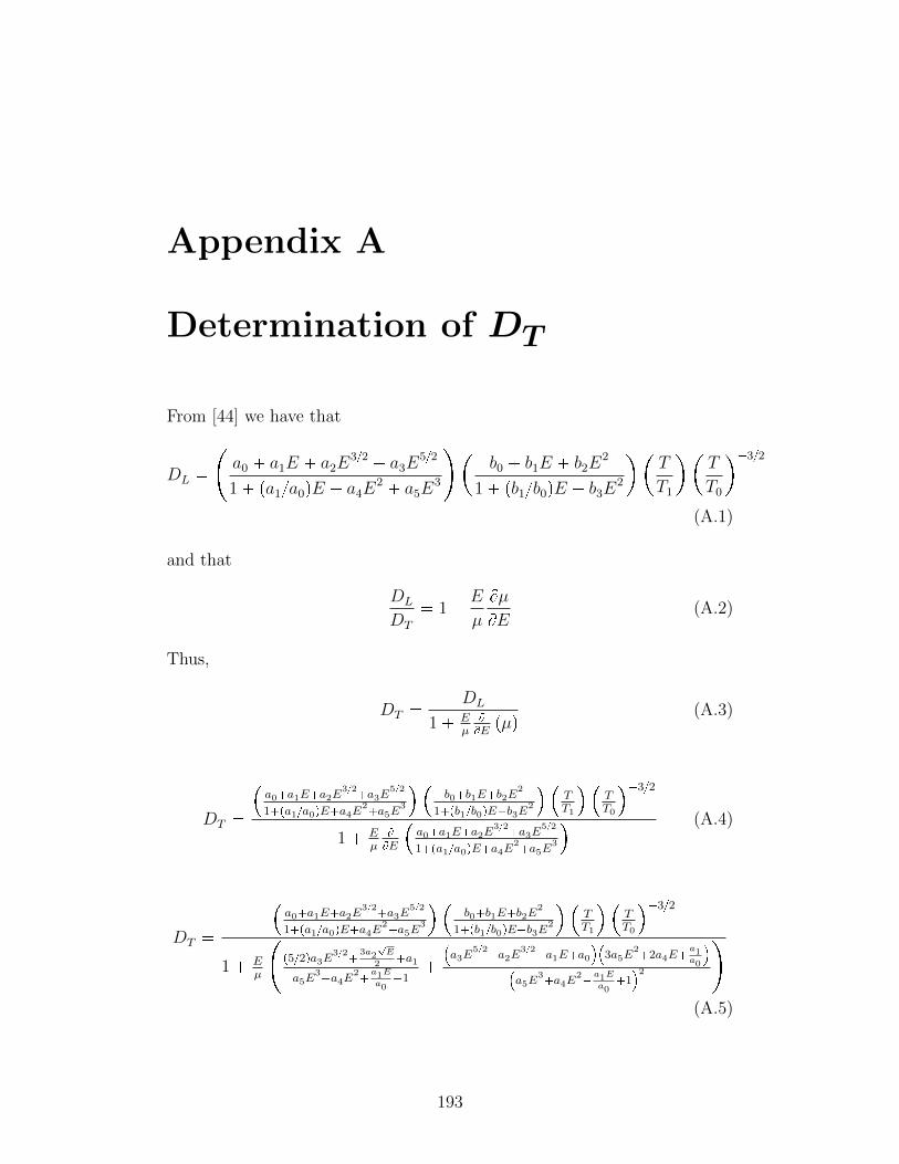
Appendix A
Determination of DT
From [44] we have that
DL a0 a1E a2E
32 a3E52
1 pa1a0qE a4E2 a5E
3
b0 b1E b2E
2
1 pb1b0qE b3E2
T
T1
T
T0
32
(A.1)
and that
DL
DT
1 E
µ
BµBE (A.2)
Thus,
DT DL
1 Eµ
BBEpµq (A.3)
DT
a0a1Ea2E
32a3E
52
1pa1a0qEa4E2a5E
3
b0b1Eb2E
2
1pb1b0qEb3E2
TT1
TT0
32
1 Eµ
BBE
a0a1Ea2E
32a3E
52
1pa1a0qEa4E2a5E
3
(A.4)
DT
a0a1Ea2E
32a3E
52
1pa1a0qEa4E2a5E
3
b0b1Eb2E
2
1pb1b0qEb3E2
TT1
TT0
32
1 Eµ
p52qa3E
32
3a2?E
2a1
a5E3a4E
2
a1E
a01
a3E
52a2E
32a1Ea0
3a5E
22a4E
a1a0
a5E
3a4E
2
a1E
a01
2
(A.5)
193
Copyright © 2022 FDOKUMEN