This is a repository copy of First results on ProtoDUNE-SP liquid argon time projection chamber performance from a beam test at the CERN Neutrino Platform.

White Rose Research Online URL for this paper:http://eprints.whiterose.ac.uk/168493/

Version: Submitted Version

Article:

Collaboration, DUNE, Abi, B, Abud, AA et al. (990 more authors) (Submitted: 2020) First results on ProtoDUNE-SP liquid argon time projection chamber performance from a beam test at the CERN Neutrino Platform. arXiv. (Submitted)

© 2020 The Author(s). For reuse permissions, please contact the Author(s).

eprints@whiterose.ac.ukhttps://eprints.whiterose.ac.uk/

Reuse

Items deposited in White Rose Research Online are protected by copyright, with all rights reserved unless indicated otherwise. They may be downloaded and/or printed for private study, or other acts as permitted by national copyright laws. The publisher or other rights holders may allow further reproduction and re-use of the full text version. This is indicated by the licence information on the White Rose Research Online record for the item.

Takedown

If you consider content in White Rose Research Online to be in breach of UK law, please notify us by emailing eprints@whiterose.ac.uk including the URL of the record and the reason for the withdrawal request.

FERMILAB-PUB-20-059-AD-ESH-LBNF-ND-SCD

CERN-EP-2020-125

First results on ProtoDUNE-SP liquid argon time

projection chamber performance from a beam test at the

CERN Neutrino Platform

The DUNE CollaborationB. Abi,142 A. Abed Abud,21,118 R. Acciarri,61 M. A. Acero,8 G. Adamov,65 M. Adamowski,61

D. Adams,17 P. Adrien,21 M. Adinolfi,16 Z. Ahmad,182 J. Ahmed,185 T. Alion,171 S. Alonso

Monsalve,21 C. Alt,53 J. Anderson,4 C. Andreopoulos,159,118 M. P. Andrews,61 F. Andrianala,2

S. Andringa,114 A. Ankowski,160 M. Antonova,77 S. Antusch,10 A. Aranda-Fernandez,39

A. Ariga,11 L. O. Arnold,42 M. A. Arroyave,52 J. Asaadi,175 A. Aurisano,37 V. Aushev,113

D. Autiero,90 F. Azfar,142 H. Back,143 J. J. Back,185 C. Backhouse,180 P. Baesso,16 L. Bagby,61

R. Bajou,145 S. Balasubramanian,189 P. Baldi,26 B. Bambah,75 F. Barao,114,92 G. Barenboim,77

G. J. Barker,185 W. Barkhouse,136 C. Barnes,125 G. Barr,142 J. Barranco Monarca,70

N. Barros,114,55 J. L. Barrow,173,61 A. Bashyal,141 V. Basque,123 F. Bay,135 J. L. Bazo Alba,152

J. F. Beacom,140 E. Bechetoille,90 B. Behera,41 L. Bellantoni,61 G. Bellettini,150 V. Bellini,33,80

O. Beltramello,21 D. Belver,22 N. Benekos,21 F. Bento Neves,114 J. Berger,151 S. Berkman,61

P. Bernardini,82,162 R. M. Berner,11 H. Berns,25 S. Bertolucci,79,14 M. Betancourt,61

Y. Bezawada,25 M. Bhattacharjee,96 B. Bhuyan,96 S. Biagi,88 J. Bian,26 M. Biassoni,83

K. Biery,61 B. Bilki,12,100 M. Bishai,17 A. Bitadze,123 A. Blake,116 B. Blanco Siffert,60

F. D. M. Blaszczyk,61 G. C. Blazey,137 E. Blucher,35 J. Boissevain,119 S. Bolognesi,20

T. Bolton,110 M. Bonesini,83,127 M. Bongrand,115 F. Bonini,17 A. Booth,171 C. Booth,164

S. Bordoni,21 A. Borkum,171 T. Boschi,51 N. Bostan,100 P. Bour,44 S. B. Boyd,185 D. Boyden,137

J. Bracinik,13 D. Braga,61 D. Brailsford,116 A. Brandt,175 J. Bremer,21 C. Brew,159

E. Brianne,123 S. J. Brice,61 C. Brizzolari,83,127 C. Bromberg,126 G. Brooijmans,42 J. Brooke,16

A. Bross,61 G. Brunetti,86 N. Buchanan,41 H. Budd,156 D. Caiulo,90 P. Calafiura,117

J. Calcutt,126 M. Calin,18 S. Calvez,41 E. Calvo,22 L. Camilleri,42 A. Caminata,81

M. Campanelli,180 D. Caratelli,61 G. Carini,17 B. Carlus,90 P. Carniti,83 I. Caro Terrazas,41

H. Carranza,175 A. Castillo,163 C. Castromonte,99 C. Cattadori,83 F. Cavalier,115 F. Cavanna,61

S. Centro,144 G. Cerati,61 A. Cervelli,79 A. Cervera Villanueva,77 M. Chalifour,21 C. Chang,28

E. Chardonnet,145 N. Charitonidis,21 A. Chatterjee,151 S. Chattopadhyay,182 P. Chatzidaki,21

J. Chaves,147 H. Chen,17 M. Chen,26 Y. Chen,11 D. Cherdack,74 C. Chi,42 S. Childress,61

A. Chiriacescu,18 K. Cho,108 S. Choubey,71 A. Christensen,41 D. Christian,61

G. Christodoulou,21 E. Church,143 P. Clarke,54 T. E. Coan,168 A. G. Cocco,85

J. A. B. Coelho,115 E. Conley,50 J. M. Conrad,124 M. Convery,160 L. Corwin,165 P. Cotte,20

L. Cremaldi,131 L. Cremonesi,180 J. I. Crespo-Anadón,22 E. Cristaldo,6 R. Cross,116

arX

iv:2

007.

0672

2v3

[ph

ysic

s.in

s-de

t] 2

3 Ju

l 202

0

C. Cuesta,22 Y. Cui,28 D. Cussans,16 M. Dabrowski,17 H. da Motta,19 L. Da Silva Peres,60

C. David,61,191 Q. David,90 G. S. Davies,131 S. Davini,81 J. Dawson,145 K. De,175 R. M. De

Almeida,63 P. Debbins,100 I. De Bonis,47 M. P. Decowski,135,1 A. de Gouvêa,138 P. C. De

Holanda,32 I. L. De Icaza Astiz,171 A. Deisting,157 P. De Jong,135,1 A. Delbart,20 D. Delepine,70

M. Delgado,3 A. Dell’Acqua,21 P. De Lurgio,4 J. R. T. de Mello Neto,60 D. M. DeMuth,181

S. Dennis,31 C. Densham,159 G. Deptuch,61 A. De Roeck,21 V. De Romeri,77 J. J. De Vries,31

R. Dharmapalan,73 M. Dias,179 F. Diaz,152 J. S. Díaz,98 S. Di Domizio,81,64 L. Di Giulio,21

P. Ding,61 L. Di Noto,81,64 C. Distefano,88 R. Diurba,130 M. Diwan,17 Z. Djurcic,4 N. Dokania,169

M. J. Dolinski,49 L. Domine,160 D. Douglas,126 F. Drielsma,160 D. Duchesneau,47 K. Duffy,61

P. Dunne,95 T. Durkin,159 H. Duyang,167 O. Dvornikov,73 D. A. Dwyer,117 A. S. Dyshkant,137

M. Eads,137 D. Edmunds,126 J. Eisch,101 S. Emery,20 A. Ereditato,11 C. O. Escobar,61

L. Escudero Sanchez,31 J. J. Evans,123 E. Ewart,98 A. C. Ezeribe,164 C. Fabre,21 K. Fahey,61

A. Falcone,83,127 C. Farnese,144 Y. Farzan,91 J. Felix,70 E. Fernandez-Martinez,122

P. Fernandez Menendez,77 F. Ferraro,81,64 L. Fields,61 A. Filkins,187 F. Filthaut,135,155

R. S. Fitzpatrick,125 W. Flanagan,46 B. Fleming,189 R. Flight,156 J. Fowler,50 W. Fox,98

J. Franc,44 K. Francis,137 D. Franco,189 J. Freeman,61 J. Freestone,123 J. Fried,17

A. Friedland,160 S. Fuess,61 I. Furic,62 A. P. Furmanski,130 A. Gago,152 H. Gallagher,178

A. Gallego-Ros,22 N. Gallice,84,128 V. Galymov,90 E. Gamberini,21 T. Gamble,164 R. Gandhi,71

R. Gandrajula,126 S. Gao,17 D. Garcia-Gamez,68 M. Á. García-Peris,77 S. Gardiner,61

D. Gastler,15 G. Ge,42 B. Gelli,32 A. Gendotti,53 S. Gent,166 Z. Ghorbani-Moghaddam,81

D. Gibin,144 I. Gil-Botella,22 C. Girerd,90 A. K. Giri,97 D. Gnani,117 O. Gogota,113 M. Gold,133

S. Gollapinni,119 K. Gollwitzer,61 R. A. Gomes,57 L. V. Gomez Bermeo,163 L. S. Gomez

Fajardo,163 F. Gonnella,13 J. A. Gonzalez-Cuevas,6 M. C. Goodman,4 O. Goodwin,123

S. Goswami,149 C. Gotti,83 E. Goudzovski,13 C. Grace,117 M. Graham,160 E. Gramellini,189

R. Gran,129 E. Granados,70 A. Grant,48 C. Grant,15 D. Gratieri,63 P. Green,123 S. Green,31

L. Greenler,188 M. Greenwood,141 J. Greer,16 W. C. Griffith,171 M. Groh,98 J. Grudzinski,4

K. Grzelak,184 W. Gu,17 V. Guarino,4 R. Guenette,72 A. Guglielmi,86 B. Guo,167

K. K. Guthikonda,109 R. Gutierrez,3 P. Guzowski,123 M. M. Guzzo,32 S. Gwon,36 K. Haaf,61

A. Habig,129 A. Hackenburg,189 H. Hadavand,175 R. Haenni,11 A. Hahn,61 J. Haigh,185

J. Haiston,165 T. Hamernik,61 P. Hamilton,95 J. Han,151 K. Harder,159 D. A. Harris,61,191

J. Hartnell,171 T. Hasegawa,107 R. Hatcher,61 E. Hazen,15 A. Heavey,61 K. M. Heeger,189

J. Heise,161 K. Hennessy,118 S. Henry,156 M. A. Hernandez Morquecho,70 K. Herner,61

L. Hertel,26 A. S. Hesam,21 J. Hewes,37 A. Higuera,74 T. Hill,93 S. J. Hillier,13 A. Himmel,61

J. Hoff,61 C. Hohl,10 A. Holin,180 E. Hoppe,143 G. A. Horton-Smith,110 M. Hostert,51

A. Hourlier,124 B. Howard,61 R. Howell,156 J. Hrivnak,21 J. Huang,176 J. Huang,25 J. Hugon,120

G. Iles,95 N. Ilic,177 A. M. Iliescu,79 R. Illingworth,61 A. Ioannisian,190 R. Itay,160 A. Izmaylov,77

E. James,61 B. Jargowsky,26 F. Jediny,44 C. Jesùs-Valls,76 X. Ji,17 L. Jiang,183 S. Jiménez,22

A. Jipa,18 A. Joglekar,28 C. Johnson,41 R. Johnson,37 B. Jones,175 S. Jones,180 C. K. Jung,169

T. Junk,61 Y. Jwa,42 M. Kabirnezhad,142 A. Kaboth,159 I. Kadenko,113 F. Kamiya,59

G. Karagiorgi,42 A. Karcher,117 M. Karolak,20 Y. Karyotakis,47 S. Kasai,112 S. P. Kasetti,120

L. Kashur,41 N. Kazaryan,190 E. Kearns,15 P. Keener,147 K. J. Kelly,61 E. Kemp,32

C. Kendziora,61 W. Ketchum,61 S. H. Kettell,17 M. Khabibullin,89 A. Khotjantsev,89

A. Khvedelidze,65 D. Kim,21 B. King,61 B. Kirby,17 M. Kirby,61 J. Klein,147 K. Koehler,188

L. W. Koerner,74 S. Kohn,24,117 P. P. Koller,11 M. Kordosky,187 T. Kosc,90 U. Kose,21

V. A. Kostelecký,98 K. Kothekar,16 F. Krennrich,101 I. Kreslo,11 Y. Kudenko,89

V. A. Kudryavtsev,164 S. Kulagin,89 J. Kumar,73 R. Kumar,154 C. Kuruppu,167 V. Kus,44

T. Kutter,120 B. Lacarelle,21 A. Lambert,117 K. Lande,147 C. E. Lane,49 K. Lang,176

T. Langford,189 P. Lasorak,171 D. Last,147 C. Lastoria,22 A. Laundrie,188 A. Lawrence,117

I. Lazanu,18 R. LaZur,41 T. Le,178 J. Learned,73 P. LeBrun,90 G. Lehmann Miotto,21

R. Lehnert,98 M. A. Leigui de Oliveira,59 M. Leitner,117 M. Leyton,76 L. Li,26 S. Li,17 S. W. Li,160

T. Li,54 Y. Li,17 H. Liao,110 C. S. Lin,117 S. Lin,120 A. Lister,188 B. R. Littlejohn,94 J. Liu,26

T. Liu,35 S. Lockwitz,61 T. Loew,117 M. Lokajicek,43 I. Lomidze,65 K. Long,95 K. Loo,106

D. Lorca,11 T. Lord,185 J. M. LoSecco,139 W. C. Louis,119 K.B. Luk,24,117 X. Luo,29 N. Lurkin,13

T. Lux,76 V. P. Luzio,59 D. MacFarland,160 A. A. Machado,32 P. Machado,61 C. T. Macias,98

J. R. Macier,61 A. Maddalena,67 P. Madigan,24,117 S. Magill,4 K. Mahn,126 A. Maio,114,55

J. A. Maloney,45 G. Mandrioli,79 J. Maneira,114,55 L. Manenti,180 S. Manly,156 A. Mann,178

K. Manolopoulos,159 M. Manrique Plata,98 A. Marchionni,61 W. Marciano,17 D. Marfatia,73

C. Mariani,183 J. Maricic,73 F. Marinho,58 A. D. Marino,40 M. Marshak,130 C. Marshall,117

J. Marshall,185 J. Marteau,90 J. Martin-Albo,77 N. Martinez,110 D.A. Martinez Caicedo ,165

S. Martynenko,169 K. Mason,178 A. Mastbaum,158 M. Masud,77 S. Matsuno,73 J. Matthews,120

C. Mauger,147 N. Mauri,79,14 K. Mavrokoridis,118 R. Mazza,83 A. Mazzacane,61 E. Mazzucato,20

E. McCluskey,61 N. McConkey,123 K. S. McFarland,156 C. McGrew,169 A. McNab,123

A. Mefodiev,89 P. Mehta,104 P. Melas,7 M. Mellinato,83,127 O. Mena,77 S. Menary,191

H. Mendez,153 A. Menegolli,87,146 G. Meng,86 M. D. Messier,98 W. Metcalf,120 M. Mewes,98

H. Meyer,186 T. Miao,61 G. Michna,166 T. Miedema,135,155 J. Migenda,164 R. Milincic,73

W. Miller,130 J. Mills,178 C. Milne,93 O. Mineev,89 O. G. Miranda,38 S. Miryala,17 C. S. Mishra,61

S. R. Mishra,167 A. Mislivec,130 D. Mladenov,21 I. Mocioiu,148 K. Moffat,51 N. Moggi,79,14

R. Mohanta,75 T. A. Mohayai,61 N. Mokhov,61 J. Molina,6 L. Molina Bueno,53 A. Montanari,79

C. Montanari,87,146 D. Montanari,61 L. M. Montano Zetina,38 J. Moon,124 M. Mooney,41

A. Moor,31 D. Moreno,3 B. Morgan,185 C. Morris,74 C. Mossey,61 E. Motuk,180 C. A. Moura,59

J. Mousseau,125 W. Mu,61 L. Mualem,30 J. Mueller,41 M. Muether,186 S. Mufson,98 F. Muheim,54

A. Muir,48 M. Mulhearn,25 H. Muramatsu,130 S. Murphy,53 J. Musser,98 J. Nachtman,100

S. Nagu,121 M. Nalbandyan,190 R. Nandakumar,159 D. Naples,151 S. Narita,102

D. Navas-Nicolás,22 N. Nayak,26 M. Nebot-Guinot,54 L. Necib,30 K. Negishi,102 J. K. Nelson,187

J. Nesbit,188 M. Nessi,21 D. Newbold,159 M. Newcomer,147 D. Newhart,61 R. Nichol,180

E. Niner,61 K. Nishimura,73 A. Norman,61 A. Norrick,61 R. Northrop,35 P. Novella,77

J. A. Nowak,116 M. Oberling,4 A. Olivares Del Campo,51 A. Olivier,156 Y. Onel,100

Y. Onishchuk,113 J. Ott,26 L. Pagani,25 S. Pakvasa,73 O. Palamara,61 S. Palestini,21

J. M. Paley,61 M. Pallavicini,81,64 C. Palomares,22 E. Pantic,25 V. Paolone,151

V. Papadimitriou,61 R. Papaleo,88 A. Papanestis,159 S. Paramesvaran,16 S. Parke,61

Z. Parsa,17 M. Parvu,18 S. Pascoli,51 L. Pasqualini,79,14 J. Pasternak,95 J. Pater,123

C. Patrick,180 L. Patrizii,79 R. B. Patterson,30 S. J. Patton,117 T. Patzak,145 A. Paudel,110

B. Paulos,188 L. Paulucci,59 Z. Pavlovic,61 G. Pawloski,130 D. Payne,118 V. Pec,164

S. J. M. Peeters,171 Y. Penichot,20 E. Pennacchio,90 A. Penzo,100 O. L. G. Peres,32 J. Perry,54

D. Pershey,50 G. Pessina,83 G. Petrillo,160 C. Petta,33,80 R. Petti,167 F. Piastra,11

L. Pickering,126 F. Pietropaolo,21,86 J. Pillow,185 J. Pinzino,177 R. Plunkett,61 R. Poling,130

X. Pons,21 N. Poonthottathil,101 S. Pordes,61 M. Potekhin,17 R. Potenza,33,80

B. V. K. S. Potukuchi,103 J. Pozimski,95 M. Pozzato,79,14 S. Prakash,32 T. Prakash,117

S. Prince,72 G. Prior,114 D. Pugnere,90 K. Qi,169 X. Qian,17 J. L. Raaf,61 R. Raboanary,2

V. Radeka,17 J. Rademacker,16 B. Radics,53 A. Rafique,4 E. Raguzin,17 M. Rai,185

M. Rajaoalisoa,37 I. Rakhno,61 H. T. Rakotondramanana,2 L. Rakotondravohitra,2

Y. A. Ramachers,185 R. Rameika,61 M. A. Ramirez Delgado,70 B. Ramson,61 A. Rappoldi,87,146

G. Raselli,87,146 P. Ratoff,116 S. Ravat,21 H. Razafinime,2 J. S. Real,69 B. Rebel,188,61

D. Redondo,22 M. Reggiani-Guzzo,32 T. Rehak,49 J. Reichenbacher,165 S. D. Reitzner,61

A. Renshaw,74 S. Rescia,17 F. Resnati,21 A. Reynolds,142 G. Riccobene,88 L. C. J. Rice,151

K. Rielage,119 A. Rigamonti,21 Y. Rigaut,53 D. Rivera,147 L. Rochester,160 M. Roda,118

P. Rodrigues,142 M. J. Rodriguez Alonso,21 J. Rodriguez Rondon,165 A. J. Roeth,50

H. Rogers,41 S. Rosauro-Alcaraz,122 M. Rosenthal,21 M. Rossella,87,146 J. Rout,104 S. Roy,71

A. Rubbia,53 C. Rubbia,66 B. Russell,117 J. Russell,160 D. Ruterbories,156 R. Saakyan,180

S. Sacerdoti,145 T. Safford,126 N. Sahu,97 P. Sala,84,21 G. Salukvadze,21 N. Samios,17

M. C. Sanchez,101 D. A. Sanders,131 D. Sankey,159 S. Santana,153 M. Santos-Maldonado,153

N. Saoulidou,7 P. Sapienza,88 C. Sarasty,37 I. Sarcevic,5 G. Savage,61 V. Savinov,151

A. Scaramelli,87 A. Scarff,164 A. Scarpelli,17 H. Schellman,141,61 P. Schlabach,61 D. Schmitz,35

K. Scholberg,50 A. Schukraft,61 E. Segreto,32 E. Seltskaya,21 J. Sensenig,147 I. Seong,26

A. Sergi,13 F. Sergiampietri,169 D. Sgalaberna,53 M. H. Shaevitz,42 S. Shafaq,104 M. Shamma,28

H. R. Sharma,103 R. Sharma,17 T. Shaw,61 C. Shepherd-Themistocleous,159 S. Shin,105

D. Shooltz,126 R. Shrock,169 L. Simard,115 N. Simos,17 J. Sinclair,11 G. Sinev,50 J. Singh,121

J. Singh,121 V. Singh,23,9 R. Sipos,21 F. W. Sippach,42 G. Sirri,79 A. Sitraka,165 K. Siyeon,36

D. Smargianaki,169 A. Smith,50 A. Smith,31 E. Smith,98 P. Smith,98 J. Smolik,44 M. Smy,26

P. Snopok,94 M. Soares Nunes,32 H. Sobel,26 M. Soderberg,172 C. J. Solano Salinas,99

S. Söldner-Rembold,123 N. Solomey,186 V. Solovov,114 W. E. Sondheim,119 M. Sorel,77

J. Soto-Oton,22 A. Sousa,37 K. Soustruznik,34 F. Spagliardi,142 M. Spanu,17 J. Spitz,125

N. J. C. Spooner,164 K. Spurgeon,172 R. Staley,13 M. Stancari,61 L. Stanco,86 D. Stefan,21

H. M. Steiner,117 J. Stewart,17 B. Stillwell,35 J. Stock,165 F. Stocker,21 T. Stokes,120 M. Strait,130

T. Strauss,61 S. Striganov,61 A. Stuart,39 R. Sulej,132,61 D. Summers,131 A. Surdo,82 V. Susic,10

L. Suter,61 C. M. Sutera,33,80 R. Svoboda,25 B. Szczerbinska,174 A. M. Szelc,123 R. Talaga,4 H.

A. Tanaka,160 B. Tapia Oregui,176 A. Tapper,95 S. Tariq,61 E. Tatar,93 R. Tayloe,98

A. M. Teklu,169 M. Tenti,79 K. Terao,160 C. A. Ternes,77 F. Terranova,83,127 G. Testera,81

A. Thea,159 J. L. Thompson,164 C. Thorn,17 S. C. Timm,61 A. Tonazzo,145 M. Torti,83,127

M. Tortola,77 F. Tortorici,33,80 D. Totani,61 M. Toups,61 C. Touramanis,118 J. Trevor,30

W. H. Trzaska,106 Y. T. Tsai,160 Z. Tsamalaidze,65 K. V. Tsang,160 N. Tsverava,65 S. Tufanli,21

C. Tull,117 E. Tyley,164 M. Tzanov,120 M. A. Uchida,31 J. Urheim,98 T. Usher,160 M. R. Vagins,111

P. Vahle,187 G. A. Valdiviesso,56 E. Valencia,187 Z. Vallari,30 J. W. F. Valle,77 S. Vallecorsa,21

R. Van Berg,147 R. G. Van de Water,119 D. Vanegas Forero,32 F. Varanini,86 D. Vargas,76

G. Varner,73 J. Vasel,98 G. Vasseur,20 K. Vaziri,61 S. Ventura,86 A. Verdugo,22 S. Vergani,31

M. A. Vermeulen,135 M. Verzocchi,61 H. Vieira de Souza,32 C. Vignoli,67 C. Vilela,169 B. Viren,17

T. Vrba,44 T. Wachala,134 A. V. Waldron,95 M. Wallbank,37 H. Wang,27 J. Wang,25 Y. Wang,27

Y. Wang,169 K. Warburton,101 D. Warner,41 M. Wascko,95 D. Waters,180 A. Watson,13

P. Weatherly,49 A. Weber,159,142 M. Weber,11 H. Wei,17 A. Weinstein,101 D. Wenman,188

M. Wetstein,101 M. R. While,165 A. White,175 L. H. Whitehead,31 D. Whittington,172

M. J. Wilking,169 C. Wilkinson,11 Z. Williams,175 F. Wilson,159 R. J. Wilson,41 J. Wolcott,178

T. Wongjirad,178 K. Wood,169 L. Wood,143 E. Worcester,17 M. Worcester,17 C. Wret,156 W. Wu,61

W. Wu,26 Y. Xiao,26 G. Yang,169 T. Yang,61 N. Yershov,89 K. Yonehara,61 T. Young,136 B. Yu,17

H. W. Yu,17 H. Z. Yu,170 J. Yu,175 Z. Y. Yu,78 R. Zaki,191 J. Zalesak,43 L. Zambelli,47

B. Zamorano,68 A. Zani,21,84 L. Zazueta,187 G. P. Zeller,61 J. Zennamo,61 K. Zeug,188

C. Zhang,17 M. Zhao,17 E. Zhivun,17 G. Zhu,140 E. D. Zimmerman,40 M. Zito,20 S. Zucchelli,79,14

J. Zuklin,43 V. Zutshi,137 and R. Zwaska61

1University of Amsterdam, NL-1098 XG Amsterdam, The Netherlands2University of Antananarivo, Antananarivo 101, Madagascar3Universidad Antonio Nariño, Bogotá, Colombia4Argonne National Laboratory, Argonne, IL 60439, USA5University of Arizona, Tucson, AZ 85721, USA6Universidad Nacional de Asunción, San Lorenzo, Paraguay7University of Athens, Zografou GR 157 84, Greece8Universidad del Atlántico, Atlántico, Colombia9Banaras Hindu University, Varanasi - 221 005, India

10University of Basel, CH-4056 Basel, Switzerland11University of Bern, CH-3012 Bern, Switzerland12Beykent University, Istanbul, Turkey13University of Birmingham, Birmingham B15 2TT, United Kingdom14Università del Bologna, 40127 Bologna, Italy15Boston University, Boston, MA 02215, USA16University of Bristol, Bristol BS8 1TL, United Kingdom17Brookhaven National Laboratory, Upton, NY 11973, USA18University of Bucharest, Bucharest, Romania19Centro Brasileiro de Pesquisas Físicas, Rio de Janeiro, RJ 22290-180, Brazil20CEA/Saclay, IRFU Institut de Recherche sur les Lois Fondamentales de l’Univers, F-91191 Gif-sur-Yvette

CEDEX, France21CERN, The European Organization for Nuclear Research, 1211 Meyrin, Switzerland22CIEMAT, Centro de Investigaciones Energéticas, Medioambientales y Tecnológicas, E-28040 Madrid,

Spain23Central University of South Bihar, Gaya – 824236, India24University of California Berkeley, Berkeley, CA 94720, USA25University of California Davis, Davis, CA 95616, USA26University of California Irvine, Irvine, CA 92697, USA27University of California Los Angeles, Los Angeles, CA 90095, USA28University of California Riverside, Riverside CA 92521, USA29University of California Santa Barbara, Santa Barbara, California 93106 USA30California Institute of Technology, Pasadena, CA 91125, USA31University of Cambridge, Cambridge CB3 0HE, United Kingdom32Universidade Estadual de Campinas, Campinas - SP, 13083-970, Brazil33Università di Catania, 2 - 95131 Catania, Italy

34Institute of Particle and Nuclear Physics of the Faculty of Mathematics and Physics of the Charles University,

180 00 Prague 8, Czech Republic35University of Chicago, Chicago, IL 60637, USA36Chung-Ang University, Seoul 06974, South Korea37University of Cincinnati, Cincinnati, OH 45221, USA38Centro de Investigación y de Estudios Avanzados del Instituto Politécnico Nacional (Cinvestav), Mexico

City, Mexico39Universidad de Colima, Colima, Mexico40University of Colorado Boulder, Boulder, CO 80309, USA41Colorado State University, Fort Collins, CO 80523, USA42Columbia University, New York, NY 10027, USA43Institute of Physics, Czech Academy of Sciences, 182 00 Prague 8, Czech Republic44Czech Technical University, 115 19 Prague 1, Czech Republic45Dakota State University, Madison, SD 57042, USA46University of Dallas, Irving, TX 75062-4736, USA47Laboratoire d’Annecy-le-Vieux de Physique des Particules, CNRS/IN2P3 and Université Savoie Mont

Blanc, 74941 Annecy-le-Vieux, France48Daresbury Laboratory, Cheshire WA4 4AD, United Kingdom49Drexel University, Philadelphia, PA 19104, USA50Duke University, Durham, NC 27708, USA51Durham University, Durham DH1 3LE, United Kingdom52Universidad EIA, Antioquia, Colombia53ETH Zurich, Zurich, Switzerland54University of Edinburgh, Edinburgh EH8 9YL, United Kingdom55Faculdade de Ciências da Universidade de Lisboa - FCUL, 1749-016 Lisboa, Portugal56Universidade Federal de Alfenas, Poços de Caldas - MG, 37715-400, Brazil57Universidade Federal de Goias, Goiania, GO 74690-900, Brazil58Universidade Federal de São Carlos, Araras - SP, 13604-900, Brazil59Universidade Federal do ABC, Santo André - SP, 09210-580 Brazil60Universidade Federal do Rio de Janeiro, Rio de Janeiro - RJ, 21941-901, Brazil61Fermi National Accelerator Laboratory, Batavia, IL 60510, USA62University of Florida, Gainesville, FL 32611-8440, USA63Fluminense Federal University, 9 Icaraí Niterói - RJ, 24220-900, Brazil64Università degli Studi di Genova, Genova, Italy65Georgian Technical University, Tbilisi, Georgia66Gran Sasso Science Institute, L’Aquila, Italy67Laboratori Nazionali del Gran Sasso, L’Aquila AQ, Italy68University of Granada & CAFPE, 18002 Granada, Spain69University Grenoble Alpes, CNRS, Grenoble INP, LPSC-IN2P3, 38000 Grenoble, France70Universidad de Guanajuato, Guanajuato, C.P. 37000, Mexico71Harish-Chandra Research Institute, Jhunsi, Allahabad 211 019, India72Harvard University, Cambridge, MA 02138, USA73University of Hawaii, Honolulu, HI 96822, USA74University of Houston, Houston, TX 77204, USA

75University of Hyderabad, Gachibowli, Hyderabad - 500 046, India76Institut de Fìsica d’Altes Energies, Barcelona, Spain77Instituto de Fisica Corpuscular, 46980 Paterna, Valencia, Spain78Institute of High Energy Physics, 100049 Beijing, China79Istituto Nazionale di Fisica Nucleare Sezione di Bologna, 40127 Bologna BO, Italy80Istituto Nazionale di Fisica Nucleare Sezione di Catania, I-95123 Catania, Italy81Istituto Nazionale di Fisica Nucleare Sezione di Genova, 16146 Genova GE, Italy82Istituto Nazionale di Fisica Nucleare Sezione di Lecce, 73100 - Lecce, Italy83Istituto Nazionale di Fisica Nucleare Sezione di Milano Bicocca, 3 - I-20126 Milano, Italy84Istituto Nazionale di Fisica Nucleare Sezione di Milano, 20133 Milano, Italy85Istituto Nazionale di Fisica Nucleare Sezione di Napoli, I-80126 Napoli, Italy86Istituto Nazionale di Fisica Nucleare Sezione di Padova, 35131 Padova, Italy87Istituto Nazionale di Fisica Nucleare Sezione di Pavia, I-27100 Pavia, Italy88Istituto Nazionale di Fisica Nucleare Laboratori Nazionali del Sud, 95123 Catania, Italy89Institute for Nuclear Research of the Russian Academy of Sciences, Moscow 117312, Russia90Institut de Physique des 2 Infinis de Lyon, 69622 Villeurbanne, France91Institute for Research in Fundamental Sciences, Tehran, Iran92Instituto Superior Técnico - IST, Universidade de Lisboa, Portugal93Idaho State University, Pocatello, ID 83209, USA94Illinois Institute of Technology, Chicago, IL 60616, USA95Imperial College of Science Technology and Medicine, London SW7 2BZ, United Kingdom96Indian Institute of Technology Guwahati, Guwahati, 781 039, India97Indian Institute of Technology Hyderabad, Hyderabad, 502285, India98Indiana University, Bloomington, IN 47405, USA99Universidad Nacional de Ingeniería, Lima 25, Perú

100University of Iowa, Iowa City, IA 52242, USA101Iowa State University, Ames, Iowa 50011, USA102Iwate University, Morioka, Iwate 020-8551, Japan103University of Jammu, Jammu-180006, India104Jawaharlal Nehru University, New Delhi 110067, India105Jeonbuk National University, Jeonrabuk-do 54896, South Korea106University of Jyvaskyla, FI-40014, Finland107High Energy Accelerator Research Organization (KEK), Ibaraki, 305-0801, Japan108Korea Institute of Science and Technology Information, Daejeon, 34141, South Korea109K L University, Vaddeswaram, Andhra Pradesh 522502, India110Kansas State University, Manhattan, KS 66506, USA111Kavli Institute for the Physics and Mathematics of the Universe, Kashiwa, Chiba 277-8583, Japan112National Institute of Technology, Kure College, Hiroshima, 737-8506, Japan113Kyiv National University, 01601 Kyiv, Ukraine114Laboratório de Instrumentação e Física Experimental de Partículas, 1649-003 Lisboa and 3004-516

Coimbra, Portugal115Laboratoire de l’Accélérateur Linéaire, 91440 Orsay, France116Lancaster University, Lancaster LA1 4YB, United Kingdom117Lawrence Berkeley National Laboratory, Berkeley, CA 94720, USA

118University of Liverpool, L69 7ZE, Liverpool, United Kingdom119Los Alamos National Laboratory, Los Alamos, NM 87545, USA120Louisiana State University, Baton Rouge, LA 70803, USA121University of Lucknow, Uttar Pradesh 226007, India122Madrid Autonoma University and IFT UAM/CSIC, 28049 Madrid, Spain123University of Manchester, Manchester M13 9PL, United Kingdom124Massachusetts Institute of Technology, Cambridge, MA 02139, USA125University of Michigan, Ann Arbor, MI 48109, USA126Michigan State University, East Lansing, MI 48824, USA127Università del Milano-Bicocca, 20126 Milano, Italy128Università degli Studi di Milano, I-20133 Milano, Italy129University of Minnesota Duluth, Duluth, MN 55812, USA130University of Minnesota Twin Cities, Minneapolis, MN 55455, USA131University of Mississippi, University, MS 38677 USA132National Centre for Nuclear Research, A. Soltana 7, 05 400 Otwock, Poland133University of New Mexico, Albuquerque, NM 87131, USA134H. Niewodniczański Institute of Nuclear Physics, Polish Academy of Sciences, Cracow, Poland135Nikhef National Institute of Subatomic Physics, 1098 XG Amsterdam, Netherlands136University of North Dakota, Grand Forks, ND 58202-8357, USA137Northern Illinois University, DeKalb, Illinois 60115, USA138Northwestern University, Evanston, Il 60208, USA139University of Notre Dame, Notre Dame, IN 46556, USA140Ohio State University, Columbus, OH 43210, USA141Oregon State University, Corvallis, OR 97331, USA142University of Oxford, Oxford, OX1 3RH, United Kingdom143Pacific Northwest National Laboratory, Richland, WA 99352, USA144Universtà degli Studi di Padova, I-35131 Padova, Italy145Université de Paris, CNRS, Astroparticule et Cosmologie, F-75006, Paris, France146Università degli Studi di Pavia, 27100 Pavia PV, Italy147University of Pennsylvania, Philadelphia, PA 19104, USA148Pennsylvania State University, University Park, PA 16802, USA149Physical Research Laboratory, Ahmedabad 380 009, India150Università di Pisa, I-56127 Pisa, Italy151University of Pittsburgh, Pittsburgh, PA 15260, USA152Pontificia Universidad Católica del Perú, Lima, Perú153University of Puerto Rico, Mayaguez 00681, Puerto Rico, USA154Punjab Agricultural University, Ludhiana 141004, India155Radboud University, NL-6525 AJ Nijmegen, Netherlands156University of Rochester, Rochester, NY 14627, USA157Royal Holloway College London, TW20 0EX, United Kingdom158Rutgers University, Piscataway, NJ, 08854, USA159STFC Rutherford Appleton Laboratory, Didcot OX11 0QX, United Kingdom160SLAC National Accelerator Laboratory, Menlo Park, CA 94025, USA161Sanford Underground Research Facility, Lead, SD, 57754, USA

162Università del Salento, 73100 Lecce, Italy163Universidad Sergio Arboleda, 11022 Bogotá, Colombia164University of Sheffield, Sheffield S3 7RH, United Kingdom165South Dakota School of Mines and Technology, Rapid City, SD 57701, USA166South Dakota State University, Brookings, SD 57007, USA167University of South Carolina, Columbia, SC 29208, USA168Southern Methodist University, Dallas, TX 75275, USA169Stony Brook University, SUNY, Stony Brook, New York 11794, USA170Sun Yat-Sen University, 510275 Guangzhou, China171University of Sussex, Brighton, BN1 9RH, United Kingdom172Syracuse University, Syracuse, NY 13244, USA173University of Tennessee at Knoxville, TN, 37996, USA174Texas A&M University - Corpus Christi, Corpus Christi, TX 78412, USA175University of Texas at Arlington, Arlington, TX 76019, USA176University of Texas at Austin, Austin, TX 78712, USA177University of Toronto, Toronto, Ontario M5S 1A1, Canada178Tufts University, Medford, MA 02155, USA179Universidade Federal de São Paulo, 09913-030, São Paulo, Brazil180University College London, London, WC1E 6BT, United Kingdom181Valley City State University, Valley City, ND 58072, USA182Variable Energy Cyclotron Centre, 700 064 West Bengal, India183Virginia Tech, Blacksburg, VA 24060, USA184University of Warsaw, 00-927 Warsaw, Poland185University of Warwick, Coventry CV4 7AL, United Kingdom186Wichita State University, Wichita, KS 67260, USA187William and Mary, Williamsburg, VA 23187, USA188University of Wisconsin Madison, Madison, WI 53706, USA189Yale University, New Haven, CT 06520, USA190Yerevan Institute for Theoretical Physics and Modeling, Yerevan 0036, Armenia191York University, Toronto M3J 1P3, Canada

E-mail: F. Cavanna (cavanna@fnal.gov), T. Junk (trj@fnal.gov), T. Yang

(tjyang@fnal.gov)

Abstract: The ProtoDUNE-SP detector is a single-phase liquid argon time projection chamber

with an active volume of 7.2 × 6.0 × 6.9 m3. It is installed at the CERN Neutrino Platform in a

specially-constructed beam that delivers charged pions, kaons, protons, muons and electrons with

momenta in the range 0.3 GeV/c to 7 GeV/c. Beam line instrumentation provides accurate mo-

mentum measurements and particle identification. The ProtoDUNE-SP detector is a prototype for

the first far detector module of the Deep Underground Neutrino Experiment, and it incorporates

full-size components as designed for that module. This paper describes the beam line, the time

projection chamber, the photon detectors, the cosmic-ray tagger, the signal processing and particle

reconstruction. It presents the first results on ProtoDUNE-SP’s performance, including noise and

gain measurements, dE/dx calibration for muons, protons, pions and electrons, drift electron life-

time measurements, and photon detector noise, signal sensitivity and time resolution measurements.

The measured values meet or exceed the specifications for the DUNE far detector, in several cases

by large margins. ProtoDUNE-SP’s successful operation starting in 2018 and its production of large

samples of high-quality data demonstrate the effectiveness of the single-phase far detector design.

Keywords: Noble liquid detectors (scintillation, ionization, single-phase), Time projection cham-

bers, Large detector systems for particle and astroparticle physics

ArXiv ePrint: 1234.56789

Contents

1 Introduction 1

2 The ProtoDUNE-SP detector 3

2.1 Cryostat 3

2.2 Time projection chamber 5

2.3 Beam plug 8

2.4 Cold electronics 9

2.5 Photon detectors 9

2.6 Cosmic-ray tagger 10

2.7 Data acquisition, timing and trigger system 11

3 CERN beam line instrumentation 14

3.1 Beam line instrumentation components 14

3.2 Beam line simulation and optimization 15

3.3 Beam line event reconstruction and particle identification 16

3.3.1 Momentum spectrometer technique/calculation 16

3.3.2 Particle identification logic 16

4 TPC characterization 17

4.1 TPC data preparation and noise suppression 17

4.1.1 Pedestal evaluation 18

4.1.2 Initial charge waveforms 18

4.1.3 Sticky code identification 19

4.1.4 ADC code mitigation 20

4.1.5 Timing mitigation 21

4.1.6 Tail removal 22

4.1.7 Correlated noise removal 23

4.2 Charge calibration 24

4.3 TPC noise level 25

4.4 Signal processing 28

4.5 Event Reconstruction 31

4.5.1 Hit finding 31

4.5.2 Pattern recognition with Pandora 33

4.6 Signal to noise performance 35

5 Photon detector characterization 37

5.1 The photon detector system 37

5.1.1 Light collectors 38

5.1.2 Photosensors 39

5.1.3 Readout DAQ and triggering 40

– i –

5.1.4 Photon detector calibration and monitoring system 41

5.2 Photosensor performance 42

5.2.1 Single photoelectron sensitivity 43

5.2.2 Signal to noise in photosensors in passive ganging configurations 45

5.2.3 Light calibration 46

5.2.4 Afterpulses and crosstalk 47

5.2.5 Response stability over time 48

5.3 Photon detector performance 48

5.3.1 Efficiency 52

5.3.2 Comparisons of cosmic-ray muons to simulation 56

5.3.3 Time resolution 57

6 TPC response 59

6.1 Space charge effects in ProtoDUNE-SP 59

6.2 Drift electron lifetime 66

6.3 Calibration based on cosmic-ray muons 70

6.3.1 Charge calibration 70

6.3.2 Energy scale calibration 72

6.4 Calorimetric energy reconstruction and particle identification 76

6.4.1 Identification and calorimetric energy reconstruction of 1 GeV/c beam pions

and muons 76

6.4.2 Identification and calorimetric energy reconstruction of 1 GeV/c beam protons 79

6.4.3 dE/dx for 1 GeV/c electrons 80

6.4.4 Particle Identification: Protons and Muons 82

7 Photon detector response 83

7.1 Calorimetric energy reconstruction from scintillation light and energy resolution 83

7.1.1 Beam electrons and EM showers 84

8 Conclusions 88

1 Introduction

The neutrino detectors at the far site of the Deep Underground Neutrino Experiment (DUNE) [1]

are planned to be built inside four cryostats, each of which will contain 17.5 kt of liquid argon (LAr).

The first detector to be constructed is planned to be a single-phase time projection chamber (TPC),

similar to, but a factor of 25 more massive than the pioneering T600 detector built by the ICARUS

collaboration [2]. The ProtoDUNE single-phase apparatus (ProtoDUNE-SP) [3], assembled and

tested at the CERN Neutrino Platform (the NP04 experiment at CERN) [4], is designed to act as

a test bed and full-scale prototype for the elements of the first far detector module of DUNE [5].

ProtoDUNE-SP contains 770 tonnes of LAr, 420 of which are in the active volume of the TPC.

– 1 –

It is currently the largest liquid argon time projection chamber (LArTPC) ever constructed. It is

designed to meet the challenges of mechanics, electronics, high voltage, cryogenics, LAr purity,

data acquisition, data storage, event reconstruction and analysis. Installation of the ProtoDUNE-SP

detector was completed in early July 2018, the filling of the cryostat with argon was completed by

mid-September 2018, and data-taking with the full apparatus started in October 2018.

In addition to its role as a demonstration prototype and engineering test bed, the ProtoDUNE-

SP TPC was exposed to a tagged and momentum-analyzed particle beam with momentum settings

ranging from 0.3 GeV/c to 7 GeV/c. This beam enabled the acquisition of large samples of data

on the behavior of charged pions, kaons, protons, muons and positive electrons (positrons) in LAr.

The beam was set to deliver only positively-charged particles for the data samples used in this

paper, although future runs will also include negatively-charged particle beams. These data serve as

templates for understanding how these particles will appear when produced in neutrino interactions

in DUNE, and they will be an important reference in the analysis of interactions in DUNE. These

data also provide a real-world test bed for the development of algorithms for pattern recognition,

event reconstruction and analysis, and they will be used to measure the cross sections of interactions

of charged particles in LAr.

The ProtoDUNE-SP apparatus is designed to satisfy the stringent new requirements and achieve

the improved levels of performance required by DUNE [6]. The membrane cryostat and its

associated cryogenic system are the largest LAr systems ever constructed. The argon purification

system is the largest constructed to date. As compared to previous devices, such as ICARUS [2],

ArgoNeuT [7], LongBo [8], MicroBooNE [9], and the 35-ton prototype [10] which had shorter

maximum drift distances, the 3.6 m drift distance in ProtoDUNE-SP makes higher demands on

argon purity. The long drift distance also requires higher voltages in the HV system used to provide

the drift field, and the stored energy which may be released in a discharge is also higher than in

previous devices. To allow for higher voltages and to reduce the chance of discharges, ProtoDUNE-

SP incorporates specially-chosen materials for the cathode and the field cage structure, and new

shapes for the field rings. The sense-wire assemblies, known as Anode Plane Assemblies (APAs),

contain three planes of readout wires on both faces and are of a novel design and construction. To

improve the signal-to-noise ratio, the sense wire readout amplifiers and analog-to-digital converters

(ADCs) are placed inside the LAr close to the wires. Furthermore, the data acquisition system

accommodates a higher data rate and larger event sizes than previous LArTPC systems.

ProtoDUNE-SP includes a novel photon-detector design which embeds the photon detectors

within the APAs in order to collect scintillation light from ionized LAr. Due to the small available

area, the photon detectors are required to be highly efficient for detecting single photons. The

performance of the photon detectors in ProtoDUNE-SP is a primary topic of this paper.

Cosmic-ray interactions with the detector cause a buildup of positive ions that drift very slowly

towards the cathode. The accumulated space charge is proportional to the rate of incident cosmic

rays and it depends strongly on the drift distance. The space charge alters the electric field in

the detector, changing both its strength and its direction, causing distortions in both the measured

positions of particles traversing the detector and their apparent ionization densities. However, the

effects of space charge buildup are expected to be largely absent in the DUNE Far Detector due to

its low cosmic-ray rate, a consequence of its deep underground location. In the analyses presented

in this paper, corrections for the effects of space charge are applied where appropriate in order for

– 2 –

the results of these studies to be generally applicable.

The ProtoDUNE-SP Technical Design Report [3] contains a detailed description of the de-

sign. A description of the apparatus as built, plus a description of the installation, testing and

commissioning is given in [11].

This paper is organized as follows. Section 2 describes different components of the ProtoDUNE-

SP detector. Section 3 describes details of the CERN beam line instrumentation. Sections 4-7

summarize results on TPC characterization, photon detector characterization, TPC response, and

photon detector response. Section 8 concludes the paper.

2 The ProtoDUNE-SP detector

The ProtoDUNE-SP apparatus, shown in figure 2, is described by a right-handed coordinate system

in which the y axis is vertical (positive pointing up) and the z axis is horizontal and points

approximately along the beam direction. The x axis is also horizontal and points along the nominal

electric field direction and is perpendicular to the wire planes1.

2.1 Cryostat

The TPC is installed in a membrane cryostat [12] with internal dimensions of 8.5 m in both the x

and z directions, and 7.9 m in y. The cryostat is filled to a height of about 7.3 m and its pressure is

maintained to 1050 mbar (absolute). The TPC is suspended by the detector support system, which

is a network of steel beams held in place by nine penetrations in the roof of the cryostat.

A detailed description of the design, construction, leak-checking, testing and validation of

the cryostat is given in [11]. The cryogenics control system is also described there. We give a

summary here of the argon purification system system that has played a crucial role in the detector

performance achieved.

The argon received from the supplier has contaminants of water, oxygen and nitrogen at the

parts per million level each. Water and oxygen will capture drifting electrons and the concentration

of these contaminants needs to be reduced by a factor of at least 104 and maintained at this level

to allow operation of the TPC. Purification of argon in the liquid phase, as required for the mass

of argon involved here, is reported in [13]. The present system builds on purification systems

developed for ICARUS and most recently at Fermilab [14] and [9], including the use of the same

filter materials. The main features of the system are indicated in figure 1. There are three circulation

loops. In one, liquid leaves the cryostat via a penetration in the side. It is pumped as liquid through

a set of filters, and it is reintroduced to the cryostat at the bottom. The pump can drive about 7 t/hr

giving a volume turnover time of about 4.5 days. In the second loop, argon gas from the purge pipes

with which each signal penetration is equipped is purified directly while warm and it is recondensed

to join the liquid flow out of the cryostat. In the third loop, the main boil-off from the argon is

recondensed directly and it then joins the liquid flow out of the cryostat. When the argon is first

circulated, the contamination level falls following a perfect mixing model with a time constant of

1Throughout this paper, the charge and energy deposited per unit track length are conventionally referred to as dQ/dx

and dE/dx respectively. The dx in these expressions is not oriented along the detector coordinate x but rather it is a

differential step along the track path.

– 3 –

the turnover time until a steady state is reached in which the rate of contamination from leaks and

outgassing from impurities balances the clean-up rate. In the NP04 cryostat, thanks to the rate of

recirculation and the avoidance of leaks, this state is equivalent to an oxygen contamination [15]

of a few parts per trillion resulting in essentially full-strength signals from the furthest parts of the

TPC.

Figure 1: A schematic of the argon purification system at NP04.

Instrumentation for monitoring the state of the argon is distributed outside the TPC near the

inner walls of the cryostat. Three purity monitors, formerly used with the ICARUS T600 detector [2],

were refurbished with new gold photocathodes and quartz fibers. They are deployed in ProtoDUNE-

SP, each at a different height. They monitor and give fast feedback on the drift electron lifetime

in the liquid argon. Two vertical columns of resistance temperature detectors (RTDs) measure

the temperature gradient of the liquid argon. Computational fluid dynamics (CFD) calculations

have been performed that predict the temperature distribution and the internal flow pattern of the

argon [16]. The temperature is predicted to vary by 15 mK total over the height of the liquid. The

RTDs have been cross calibrated in situ to better than 2 mK and their measurements agree with

the predictions within ±3.7 mK. A set of cameras and LED lights in the liquid and in the ullage

provides monitoring of the mechanical state of the apparatus during filling and operation.

– 4 –

2.2 Time projection chamber

Figure 2 shows a view of the TPC with its major components labeled and a photo of one of the

two drift volumes. The active region of the TPC encloses a volume 6.0 m high, 6.9 m along the z

direction, and 7.2 m in the x direction. The TPC is divided into two separate half-volumes with a

solid, planar cathode at x = 0 in the yz plane, with three APAs 3.6 m from the cathode on either

side.

The cathode plane of the TPC is formed from six cathode plane assemblies (CPAs). Each CPA

is 1.15 m wide and 6.1 m high, and consists of three vertically stacked cathode panels. The stored

electrical energy in the TPC when fully charged presents a challenge. If the cathode were electrically

conducting, an electrical breakdown can discharge it rapidly, endangering the front-end electronics.

Instead, the cathode is constructed out of resistive materials which give it a very long discharge time

constant, reducing the risk. The CPA panels are constructed from FR4, a fire-retardant fiberglass-

epoxy composite material. These panels are laminated on both sides with a commercial Kapton

film with a resistivity of ∼3.5 MΩ/sq. The cathode plane is biased at -180 kV to provide a 500 V/cm

drift field. A field cage with 60 voltage steps on each side of the cathode ensures the uniformity

of the nominal drift field between the cathode plane and the sense planes. The electric field differs

from the nominal prediction due to space-charge effects, which are described in section 6.1.

A sketch of an APA is shown in figure 3. Each APA has a rectangular stainless steel frame

6.1 m high, 2.3 m wide, and 76 mm thick. There are four layers (planes) of wires bonded on each

side of the frame. The wire planes and their wire orientations are (from outside in) the Grid (G)

layer (vertical), the U layer (+35.7 from vertical), the V layer (-35.7 from vertical), and the X layer

(vertical). A bronze wire mesh with 85% optical transparency is bonded directly over each side of

the APA frame to provide a grounded shield plane for the four wire planes mentioned above. Each

successive wire plane is built 4.75 mm above the previous layer, including the wire mesh. The wires

are terminated on wire boards which are stacked on the short ends the APA. The G and X layers

have the same wire pitch of 4.79 mm, but are staggered by half a wire pitch in relative position. The

U and V wires have a pitch of 4.67 mm. Wires on the two induction planes are helically wrapped

around the frame from the head, to the sides, and then to the foot. Wires are held in place with FR-4

boards with teeth cut in them as they wrap around the sides. The wire angle is chosen such that the

wires do not wrap more than one revolution to avoid creating ambiguities in track reconstruction.

Four wire support combs made out of 0.5 mm-thick G10 (a fiberglass-epoxy composite material)

are installed on each side of each APA uniformly spaced along the y direction, in order to hold

the long wires in place, helping to counteract gravitational, electrostatic, and fluid-flow forces that

would otherwise cause portions of the wires to be displaced from their nominal positions. Each

wire plane is electrically biased at a different potential such that the primary ionization electrons

created in the drift volume pass through the G, U and V planes without being captured, and finally

are collected on the X wires. Therefore, the X plane wires are also referred to as the collection

wires, and the U, V plane wires as the first and second induction plane wires. The grid plane wires

serve as an electrostatic discharge (ESD) protective shield and are not read out. The nominal wire-

plane bias voltages, to ensure electron collection only on collection-plane wires, are VG = −665 V,

VU = −370 V, VV = 0 V, VX = +820 V.

The G plane on the lowest-z APA on the x < 0 side of the detector was unintentionally not

– 5 –

Figure 2: Top: a view of the TPC with its major components labeled; bottom: a photo of one of

the two drift volumes, where three APAs are on the left side and the cathode is on the right side.

connected to its voltage supply. The break in connectivity was determined to be inside the cryostat

– 6 –

Figure 3: Sketch of a ProtoDUNE-SP APA, showing portions of the U (green), V (magenta), the

induction layers; and X (blue), the collection layer, to accentuate their angular relationships to the

frame and to each other. The induction layers are connected electrically across both sides of the

APA. The grid layer (G) wires (not shown), run vertically, parallel to the X layer wires. Separate

sets of G and X wires are strung on the two sides of the APA. From ref. [3].

and it could not be repaired for the duration of the run. Groups of four G plane wires are connected

to a 3.9 nF capacitor with the other terminal grounded. Without a voltage supply, drifting ionization

electrons will charge up the G-plane from its initial state to a potential that repels electrons and

prevents further charge collection. This charging process takes approximately 100 hours [5], and

the average charge measured by this APA is reduced during the charge-up time.

Electron diverters are installed in the two vertical gaps between the APAs on the negative-x

side of the cathode, but not between the APAs on the positive-x side. These diverters consist of

two vertical electrode strips, an inner electrode and an outer electrode, mounted on an insulating

board that protrudes approximately 25 mm into the drift volume beyond the G plane wires. Voltages

applied to the diverter electrodes modify the local drift field so that electrons drift away from the gaps

between the APAs and into the active area. A diagram showing the field lines and equipotentials

in the vicinity of the electron diverters when they are working as designed is given in ref. [3].

– 7 –

High currents were drawn from the electron diverters’ power supplies when they were energized,

due to one or more electrical shorts in the cold volume. The electron diverters were therefore left

unpowered. A resistive path to ground on each one ensured that the actual voltage on the outer

electrode was close to zero, which was not the intended voltage. The grounded diverter electrodes

collected charge near the gaps, and also distorted nearby drift paths.

2.3 Beam plug

The test beam enters the detector at mid-height and about 30 cm away from the cathode, on the

negative x side. It points down 11 from the horizontal, and towards the APA on the negative x side,

10 to the right of the z direction. In order to minimize the energy loss of beam particles prior to

their entry in the TPC due to the materials in the cryostat, the 40 cm of inactive liquid argon in front

of the TPC, and the field cage, a “beam plug” [3] is installed on the low-z, negative-x side of the

end-wall field cage, as shown in figure 4. This beam plug is constructed from a series of alternating

fiberglass and stainless steel rings to form a cylinder, and capped at entrance and exit ends with low

mass fiberglass plates. The stainless steel rings are connected to three sets of resistors to regulate

the voltage from the field cage to the grounded cryostat membrane. The beam plug extends through

an opening in the field cage about 5 cm inside the field cage boundary. The inside face of the beam

plug is covered with a mini field cage made from 0.8 mm thick printed circuit board to reduce the

drift field distortion introduced by this opening. The beam plug is filled with nitrogen at a nominal

pressure of 1.3 bar (absolute pressure) to balance the hydrostatic pressure of the liquid argon at this

height and also to maintain high dielectric strength to avoid HV breakdown. Besides, the cryostat

warm structure and the insulation are also modified to reduce the beam interaction with passive

materials.

~50cm

Nitrogen Line &

Electrical Ground

Glass-Epoxy

Ring Section

Secondary Beam

Plug SupportHV Connection

Profile #5

Mounting FlangeGrading

Resistors (18x)

Grading Rings (7x)

Ground Potential

Beam

Figure 4: Drawing of the beam plug (left) and an image of the beam plug installed inside the

cryostat (right).

– 8 –

2.4 Cold electronics

The U, V and X wire planes on both sides of an APA are read out by 20 front-end motherboards

(FEMBs) installed close to the wire boards on top of each APA. The FEMBs amplify, shape, digitize,

and transmit all 15,360 TPC channels’ signals to the warm interface electronics through cold data

cables, which are up to 7 m in length. Each FEMB contains one analog motherboard, which is

assembled with eight 16-channel analog front-end (FE) ASICs [17], to provide amplification and

pulse shaping, and eight 16-channel Analog to Digital Converter (ADC) ASICs for a total of 128

channels readout per FEMB.

Each FE ASIC channel has a dual-stage charge amplifier circuit with a programmable gain

selectable from 4.7, 7.8, 14 and 25 mV/fC, and a 5th-order anti-aliasing shaper with a programmable

time constant with peaking times of 0.5, 1, 2, and 3 µs. The FE ASIC also has an option to enable

AC coupling and a baseline adjustment for operation at either 200 mV for the unipolar pulses on

the collection wires or 900 mV for the bipolar pulses on the induction wires. Under normal running

conditions the ASIC gain is set at 14 mV/fC and the peaking time is set at 2 µs for all channels.

On October 11, 2018, the internal ASIC baseline was changed to 900 mV for both induction and

collection channels in order to mitigate ASIC saturation with large input charge. Each FE ASIC also

has an adjustable pre-amplifier leakage current selectable from 100, 500, 1000, and 5000 pA. The

default leakage current is 500 pA. The estimated power dissipation of a FE ASIC is about 5.5 mW

per channel at 1.8 V. Each FE ASIC contains a programmable pulse generator with a 6-bit DAC for

electronics calibration, which is connected to each channel individually via an injection capacitor.

The ADC ASIC has 16 independent 12-bit digitizers performing at speeds up to 2 megasamples

per second (MS/s).

A commercial Altera Cyclone IV FPGA, assembled on a mezzanine card that is attached to

the analog motherboard, provides clock and control signals to the FE and ADC ASICs. The FPGA

also serializes the 16 data streams from the ADCs into four 1.25 Gbps links for transmission to the

warm interface electronics over the cold data cables. The FPGA can also provide a calibration pulse

to each FE ASIC channel via the same injection capacitor used for the internal FE ASIC DAC, as

a cross-check for the electronics calibration. The production, commissioning and performance of

the cold electronics components are described in [18].

The number of TPC channels that do not respond to charge signals from cosmic-ray muons

evolved over the course of the data-taking period. Twenty-nine channels never showed any sensitivity

to signals, from September 2018 to January 2020. An additional seven became solidly unresponsive

during the run, making the total unresponsive channel count 36 in January 2020. Approximately

30 additional channels were found to be intermittently unresponsive during the run. During initial

cold-box testing before installation, 34 channels were identified as non-responsive; this includes the

29 initially dead channels and five intermittent ones that happened to be non-responsive during the

test.

2.5 Photon detectors

Liquid argon is a prolific emitter of scintillation light. Approximately 2.4×104 vacuum ultraviolet

(VUV) photons are created per MeV of energy deposited by ionization in LAr at the nominal electric

– 9 –

field of 500 V/cm. Photon detectors are installed in ProtoDUNE-SP in order to detect a fraction

of these photons to measure interaction times and to get an independent measurement of deposited

energy. These photon detectors, however, cannot be placed outside of the field cage because it

blocks the scintillation light, and so the photon detectors are integrated in the APAs, occupying the

space between the two mesh planes. Ten bar-shaped photon detectors with dimensions of 8.6 cm

(height) 2.2 m (length) and 0.6 cm (thickness) are embedded at equally spaced heights within each

APA. A number of different designs of photon-detector technologies are implemented within this

size constraint. In each design, silicon photomultipliers [19] are used to convert the light to electrical

signals, which are brought out of the cryostat on copper cables. Most of the photon detectors sense

the light that reaches the ends of the bars – the exception is the so-called ARAPUCA design, which

collects light at several positions along the bar. More details on the photon detector system are

provided in section 5.

2.6 Cosmic-ray tagger

The CRT is a system of scintillation counters that covers almost the entire upstream and downstream

faces of the TPC. It was installed in order to provide triggers to read out the detector for a set of

cosmic-ray muons that pass through with known timing and direction, parallel to the TPC readout

planes. Since the ProtoDUNE-SP detector is on the surface, it is exposed to 20 kHz of cosmic-ray

muons. Most of these muons are not tagged before entry into the TPC. Both untagged muons

and muons tagged by the CRT are exploited to provide important calibration data and performance

indicators.

The CRT uses scintillation counters recycled from the outer veto of the Double Chooz exper-

iment [20]. It is constructed in four large assemblies, two mounted upstream and two mounted

downstream of the cryostat. Each assembly covers an area approximately 6.8 m high and 3.65 m

wide. The CRT uses 32 modules containing 64 scintillating strips each. The strips are 5 cm wide

and 365 cm long. The strips in each module are parallel to each other, and thus a module provides a

one-dimensional spatial measurement for each track at a given position along z. In order to enable

two-dimensional sensitivity in x and y, four modules are placed together into eight assemblies with

two modules being rotated by 90 degrees to create an assembly of 3.65 m by 3.65 m in size, as

shown in figure 5. Four of these units are placed to cover the upstream (front) face of the detector

and the other four placed against the downstream (back) face. Hamamatsu M64 multi-anode pho-

tomultiplier tubes detect the scintillation light and the resulting electrical pulses are digitized by

ADCs and recorded by the data acquisition system along with timestamps with 20 ns resolution.

A digitized pulse and its timestamp are called a “one-dimensional hit”. Two-dimensional hits are

reconstructed when two one-dimensional hits are recorded in overlapping CRT modules within a

coincidence window of 80 ns. A cosmic-ray muon track is reconstructed in the CRT by drawing a

line from hits in the front modules to hits in the back modules within a coincidence window dictated

by the estimated time of flight to travel from the front modules to the back modules.

Half of the 32 upstream CRT modules cover the upstream face of the detector and the other half

of the CRT modules cover the downstream face of the detector as seen in figure 6. The upstream

CRT modules are offset due to the beam pipe, which enters the cryostat at an angle. Because of this,

eight CRT modules cover the area near the cathode along the x direction, but 9.5 m upstream from

– 10 –

Figure 5: Drawing of CRT modules overlaid (left) and an image of CRT modules installed

downstream (right). Two CRT modules measure the x coordinate and two CRT modules are rotated

to measure the y coordinate.

the front face of the TPC. The other eight upstream CRT modules sit to the left of the beam pipe

with an offset of 2.5 m upstream from the from face of the TPC. The downstream CRT modules are

centered with respect to the center of the TPC in x and sit 10 m downstream from the front face of

the TPC.

2.7 Data acquisition, timing and trigger system

The ProtoDUNE-SP data acquisition system (DAQ) is responsible for reading the data from the

TPC, the photon detector and the CRT. It also reduces the data volume using online triggering and

compression techniques and formats the data into trigger records2 for storage and offline processing.

The TPC has two candidate readout solutions under test in ProtoDUNE-SP: RCE (ATCA-based) [21]

and FELIX (PCIe-based) [22]. Both of these systems ran simultaneously. For the beam runs, five

out of the six APAs were read out using RCEs and one APA was read out using FELIX. After the

beam runs, four APAs were converted from RCE readout to FELIX readout. Fermilab’s artDAQ [23]

is used as the data-flow software.

The ProtoDUNE-SP timing system provides a 50 MHz clock multiplexed on an 8b10b encoded

data stream that is broadcast to all endpoints. The timing system interfaces to the CERN SPS beam

presence signals and can be used to switch modes for data taking with and without beam. The

timing system data stream also provides the trigger distribution. The timing system is partitionable,

a feature that allows parts of the experiment to run independently. A clock synchronized to the

2The word “event” is customarily used for a triggered detector readout in many high-energy physics experiments. Due

to the need to refer to interactions as events and the presence of multiple interactions per detector readout, we standardize

on “trigger record” as the name of a unit of data produced by the DAQ.

– 11 –

Figure 6: Installation of the Cosmic Ray Tagger (CRT): (top) 3D view with staggered upstream

modules visible in front of the cryostat, (bottom-left) side view, (bottom-right) top view, with

positions of the staggered upstream modules and downstream parallel modules indicated by labels.

Global Positioning System provides 64-bit timestamps that are used to mark the trigger and data

times irrespective of file name, run, or trigger record numbers.

A hardware triggering system was designed in order to perform event selection in ProtoDUNE-

SP. The core element of this system is the Central Trigger Board (CTB) which is a custom printed

circuit board (PCB) in charge of processing the status of the auxiliary detectors to aid in making

prompt readout decisions. The readout decisions are ultimately made by the timing system which

communicates with the CTB through various commands. The CTB hosts a MicroZed, which is a

commercial PCB with an onboard System-On-a-Chip (SoC). The SoC contains both Programmable

Logic (PL) and a Processing System (PS) and serves as an interface between the auxiliary detectors

(photon detectors, beam instrumentation, and CRT) and the DAQ through the timing system. The

CTB has 32 individual CRT pixel inputs (a pixel being a unit of two overlapping panels), 24 optical

inputs for the photon detection system, and seven inputs for beam instrumentation signals, all of

which are translated into digital pulses and forwarded to the PL for further processing.

The CTB triggering firmware operating in the PL is organized into a two-level hierarchy of

low-level and high-level triggers (LLTs and HLTs) which are configurable at run-time by the DAQ

system. LLTs are defined for inputs from a single subsystem while HLTs can be defined using

the various LLTs and can therefore span any or a combination of the subsystems. Several trigger

conditions can be set up; each one is uniquely identified by a bitmask and is embedded into a trigger

– 12 –

word issued to the DAQ. An overview of the CTB trigger scheme and its interface with the DAQ is

depicted in figure 7.

Figure 7: CTB trigger hierarchy.

Additionally, multiple trigger conditions can be satisfied during a single triggered detector

readout. To distinguish between these, the CTB timestamps all LLTs and HLTs generated with the

50 MHz system clock. This (64-bit) timestamp is also included in the trigger word along with the

bitmask.

In the HLT, trigger conditions can be configured to require coincidences or anti-coincidences

between the various LLTs. Only when all the required conditions for an HLT are satisfied is a

trigger command passed to the timing system. The timing system is then responsible for validating

or vetoing3 the issued trigger. If accepted, the timing system forwards the readout decision to

the DAQ software and to the individual readout systems (i.e. TPC, photon detectors, and CRT).

However, for accountability4, the CTB sends a data word directly to the DAQ to be stored regardless

of whether or not the trigger is validated by the timing system.

All HLTs can be classified as beam-on or beam-off triggers. The former relies mostly on

the beam instrumentation inputs and requires the conditions to be satisfied during a beam spill

while the latter requires that the conditions are satisfied outside the beam spill. The most common

examples of beam-on triggers include those aimed at tagging electron, proton and kaon events.

By requiring different signal combinations from the beam instrumentation inputs, one can identify

specific particles for a relevant energy range, which will be discussed in section 3.

3In case a trigger has already been issued by the timing system.4If beam pile-up occurs, the timing system vetoes any additional beam triggers if it has issued one in the last 10 ms.

However, the CTB still reports multiple beam triggers in this case.

– 13 –

The most common examples of beam-off triggers are those arising from cosmic-ray activity.

Several of these triggers are in place to select events with specific topologies, requiring CRT pixels

from specific regions to register hits in coincidence with pixels from another region. For example,

by requiring that at least one upstream CRT pixel is hit in coincidence with a downstream CRT

pixel, one can select throughgoing muon candidates. Another trigger is set up for cathode-crossing

muon candidates, which is achieved by requiring coincidence hits on CRT pixels on opposing drift

volumes and sides of the cryostat. In addition to the logic-specific triggers, an aperiodic random

trigger is provided to read out the detector without regard to trigger conditions.

For each triggered readout of the detector, the TPC data consists of 6000 consecutive samples

of each ADC, which are digitized at a rate of 2 MHz, for a total of 3 ms of time. Each time period

of 500 ns between ADC samples is called a “tick." The data readout starts 250 µs (500 ticks) before

the trigger time in order to collect charge deposited by particles that arrive earlier than the trigger

but cause charge to arrive at the anodes during time periods that overlap those of triggered events.

Corresponding data from the photon detectors and the CRT are saved in the output data stream for

analysis. Compressed raw data trigger records have a typical size of 60 MB, and trigger rates of

40 Hz were reliably sustained by the data acquisition system. A typical physics run lasts several

hours.

3 CERN beam line instrumentation

The ProtoDUNE-SP TPC is located in the CERN North Area in a tertiary extension branch of

the H4 beam line. The 400 GeV/c primary proton beam is extracted from the CERN Super

Proton Synchrotron (SPS) and is directed towards a beryllium target, producing a mixed hadron

beam with a momentum of 80 GeV/c. This secondary beam is then transported to impinge on a

secondary target, producing a tertiary, very low energy (VLE) beam in the 0.3 - 7 GeV/c momentum

range. The H4-VLE beam line then accepts, momentum-selects and transports these particles to

the ProtoDUNE-SP detector. The secondary target material can be changed between copper and

tungsten. The latter is chosen for momenta below 4 GeV/c in order to increase the hadron content

of the beam. However, the copper target was unintentionally used for the 2 GeV/c run instead of

the tungsten target.

3.1 Beam line instrumentation components

The H4-VLE beam line is instrumented with three types of detectors that provide particle identifi-

cation and a trigger for the TPC. There are eight profile monitors (“XBPF”), three trigger counters

(“XBTF”) and two threshold Cherenkov counters (“XCET”). There are also three bending magnets

that direct the beam toward the ProtoDUNE-SP detector. The second of these magnets is also used

as part of a momentum spectrometer. The relative positions of each of these features can be seen in

figure 8. A description of the beam line design has been reported elsewhere [24], while an in-depth

discussion of the instrumentation can be found in [25].

The XBPFs, described in detail in [26], are scintillating fiber detectors, each containing

192 square fibers, approximately 1 mm thick. The fibers are arranged in a planar configuration

and cover an area of approximately 20 × 20 cm2. Each device contains a single plane of fibers

– 14 –

ProtoDU

NE

-SP

Time of Flight

Momentum Spectrometer Beam line Trigger

28.575 m

XBTF XBPF

XCET

XBPF XBTF

XBTF XBPF

Figure 8: A schematic diagram showing the relative positions of the trigger counters (XBTFs),

bending magnets (triangles), profile montiors (XBPFs) and Cherenkov detectors (XCETs) in the

H4-VLE beam line. Combining data from different pieces of instrumentation can be used for

triggering, reconstructing momentum and measuring time of flight.

and therefore measures one spatial coordinate. Pairs of these detectors, rotated by 90° with respect

to each other, are placed at several points along the beam line. This arrangement allows the

beam position to be tracked on a particle-by-particle basis. The XBPF data is also used in the

reconstruction of a particle’s momentum, discussed in section 3.3.1. Hits in the last two sets of

XBPF devices are used to measure the trajectories of the beam particles that are then extrapolated

to the face of the ProtoDUNE-SP TPC. The XBTFs are designed in a similar way. However, instead

of each fiber being read out separately, they are gathered into two bundles and therefore offer no

position resolution. Instead, the signals from upstream and downstream planes, which are separated

by 28.575 m, are connected to a time-to-digital converter (FMC-TDC [27]). The TDC signals from

these two planes provide a particle’s time of flight (TOF). The resolution of this measurement has

been measured to be approximately 900 ps [25].

Coincident signals from the middle and downstream XBTFs act as a “general trigger.” These

general triggers are sent to the CTB serving as conditions for HLTs as described in section 2.7.

During data taking across the momentum regime of interest, the measured efficiencies of the XBPFs

with respect to these triggers are greater than 95% for all chambers [25].

The two Cherenkov counters used in the H4-VLE are of similar design [28, 29], although one

is able to sustain a higher radiator gas pressure. The internal pressures of the two devices were

tuned to tag different particle species at various momenta. A combination of the TOF and the

two Cherenkov signals (high and low pressure), offers particle identification for analysis across the

whole momentum spectrum of interest. During the beam run, signals from these devices were sent

to the CTB to form HLTs tagged as various beam particle species.

3.2 Beam line simulation and optimization

The beam transported in the H4-VLE beam line is produced by the collision of the secondary

mixed hadron beam of 80 GeV/c with the secondary fixed target. To limit the contributions from

the decays of unstable low-energy hadrons such as pions and kaons, a beam line length of less

than 50 m is required. Low-energy beam particles need to be sufficiently separated from the high-

– 15 –

energy background in this distance, and enough space for the beam line instrumentation is required.

Detailed simulation studies were carried out in order to meet these specifications.

The performance of the initial layout was calculated with the beam optics code Transport [30]

and refined by a comprehensiveMAD-X [31] (andMAD-X-PTC [32]) simulation [33]. The Monte Carlo

simulations use two frameworks, G4beamline [34] and FLUKA [35, 36]. Different target lengths

and materials were investigated to satisfy the experimental needs of rate and beam composition.

The target choice (either copper or tungsten) and the different field strengths of the beam line’s

dipoles and quadrupoles are incorporated into the G4beamline and FLUKAmodels. Based on these

studies, estimates of the beam rates, compositions and background rates at the experiment location

are obtained. The background suppression was improved by optimizing the shielding using the

FLUKA simulation [25].

3.3 Beam line event reconstruction and particle identification

Information from the three types of beam line instruments (discussed in section 3.1) is combined

in order to perform particle identification on an event-by-event basis. A search window in time of

500 ns is defined around each general trigger; timestamps associated with data packets from each

device are then matched within this interval.

3.3.1 Momentum spectrometer technique/calculation

The three XBPF detectors surrounding the middle bending magnet provide a measurement of each

particle’s momentum. This is illustrated in figure 9 [28]. The lateral position of the particle at each

XBPF detector (χ1, χ2, χ3) is provided by the index of the activated fibers in the profile monitors.

These measurements, along with the known distances between the monitors (L1, L2, L3) and the

measured magnetic field are used with equations 3.1 and 3.2 to determine a particle’s bending angle

θ and momentum p.

cos θ =M[∆L tan θ0 + ∆χ cos θ0] + L1∆L

√[M2+ L2

1][(∆L tan θ0 + ∆χ cos θ0)2 + ∆L2]

(3.1)

p =299.7924

θ×

∫ Lmag

0

(Bdl) (3.2)

Here, M ≡ α + χ1, α = χ3L2−χ2L3

L3−L2cos θ0, ∆L ≡ L3 − L2, and ∆χ ≡ χ2 − χ3. θ0 is the nominal

bending angle of the beam and is equal to 120.003 mrad [25].

3.3.2 Particle identification logic

The beam line is designed to provide particle identification (PID) for the various particle types (p,

µ, π, e, K) comprising the beam. Depending on the beam momentum settings, different conditions

are applied to the data from the beam line instrumentation to extract the particle types. These

conditions are listed in table 1. This technique is demonstrated for selected runs at various beam

momenta in figures 10(a) – 10(d). Figure 11 shows the measured momentum and TOF distribution

throughout the selected runs. The red curves show expected TOF for several particle types (e, µ, π,

– 16 –

the measured Δp/p

mm and 0.8 mm we obtain a Δp/p of 1.1%, 2.5% and 3.9%

Δp/p deteriorates

Figure 9: A schematic diagram showing the method by which momentum is reconstructed for a

given beam particle (red), as discussed in the text. Taken from [28]. The direction of the x axis is

opposite to the convention used in this paper.

K , p and d) given the particle’s momentum, its mass, and assuming a distance of 28.575 m between

the TOF monitors.

4 TPC characterization

The large quantities of high-quality data collected by ProtoDUNE-SP enable many studies of the

performance of the TPC. This section describes the offline data preparation and noise suppression,

charge calibration, noise measurement, signal processing, event reconstruction, signal-to-noise

performance, and a measurement of the electron lifetime.

4.1 TPC data preparation and noise suppression

The ProtoDUNE-SP detector is typically triggered at a rate of 1-40 Hz where each trigger record

includes synchronized contiguous samples from all TPC channels, typically with a length of 3 ms

corresponding to 6000 ticks (ADC samples). Trigger records are processed independently of

one another, beginning with data preparation which converts the ADC waveform (ADC count for

each tick) for each channel to a charge waveform. The data preparation comprises evaluation

of pedestals, charge calibration, mitigation of readout issues, tail removal and noise suppression.

These operations are necessary in order to optimize the performance of subsequent stages of event

reconstruction. The data preparation steps are described in detail in the following subsections.

– 17 –

Table 1: A summary of beam line instrumentation logic used in the identification of particle types.

Each cell reflects how a particular type of instrumentation is used at a given reference momentum.

When time of flight is used, the values of the lower and upper cuts are given in nanoseconds. In

the case of the high-pressure Cherenkov (XCET-H) and the low-pressure Cherenkov (XCET-L),

zero and one represent the absence and presence of a signal respectively. When a given piece of

instrumentation is not involved in a logic decision at a given momenta, a dash is used.

Momentum (GeV/c)

1 2 3 6 - 7

e

TOF (ns) 0, 105 0, 105 – –

XCET-L 1 1 1 1

XCET-H – – 1 1

µ / πTOF (ns) 0, 110 0, 103 – –

XCET-L 0 0 0 1

XCET-H – – 1 1

K

TOF (ns) – – – –

XCET-L – – 0 0

XCET-H – – 0 1

p

TOF (ns) 110, 160 103, 160 – –

XCET-L 0 0 0 0

XCET-H – – 0 0

4.1.1 Pedestal evaluation

Voltage offsets are introduced at the inputs to the amplifier and ADC for each channel to keep

the signals in the appropriate range for each of these devices. These offsets and the gains of both

devices vary from channel to channel and so there are channel-to-channel variations in the ADC

pedestal, i.e. the mean ADC count that would be observed in the absence of signal. In addition, the

pedestal is observed to have significant variation from one trigger record to another, presumably

due to low-frequency (compared to the 3 ms readout window) noise pickup before the amplifier. To

cope with this, the pedestal is evaluated independently for each channel and each trigger record.

The pedestal is evaluated by histogramming the ADC count for all (typically 6000) ticks and

fitting the observed peak with a Gaussian whose mean is used as the pedestal. The RMS of the

fit Gaussian provides an initial estimate of the noise in the channel and is typically around four

to six ADC counts. Due to the sticky-code issues described in section 4.1.3, these ADC count

distributions are sometimes observed to have spikes at the offending sticky codes which can bias

the pedestal estimate. To reduce this bias, the peak bin is excluded from the fit if it holds more than

20% of the samples.

4.1.2 Initial charge waveforms

Initial charge waveforms are obtained for each channel by subtracting the pedestal from each of the

ADC counts and multiplying this difference by the gain assigned to the channel. These gains may

– 18 –

Time of Flight [ns]80 100 120 140 160

Rela

tive F

requency

0.0

0.2

0.4

0.6

0.8

1.0e

π / µp

DUNE:ProtoDUNE-SP Beam Line Data (1 GeV/c)

(a) Nominal beam momentum = 1 GeV/c. Verti-cal lines represent the time of flight cuts used forelectrons (blue), and muons/pions (red).

Time of Flight [ns]85 90 95 100 105 110 115

Rela

tive F

requency

0.0

0.2

0.4

0.6

0.8

1.0e

π / µp

DUNE:ProtoDUNE-SP Beam Line Data (2 GeV/c)

(b) Nominal beam momentum = 2 GeV/c. Verti-cal lines represent the time of flight cuts used forelectrons (blue), and muons/pions (red).

Time of Flight [ns]85 90 95 100 105 110

Rela

tive F

requency

0.0

0.2

0.4

0.6

0.8

1.0e

π / µp/K

DUNE:ProtoDUNE-SP Beam Line Data (3 GeV/c)

(c) Nominal beam momentum = 3 GeV/c.

Time of Flight [ns]85 90 95 100 105

Rela

tive F

requency

0.0

0.2

0.4

0.6

0.8

1.0π / µe /

K

p

DUNE:ProtoDUNE-SP Beam Line Data (6 GeV/c)

(d) Nominal beam momentum = 6 GeV/c.

Figure 10: Time of flight distributions for different reference momenta, separated by particle using

the PID techniques listed in table 1. The distributions are normalized such that the maximum height

is equal to 1.

be set to 1.0 to obtain a charge waveform in units of ADC counts or they may be taken from a charge

calibration. The standard ProtoDUNE-SP reconstruction makes use of the calibration discussed in

section 4.2.

Figure 12(a) shows an example event display consisting of waveforms on wires in the collection

plane of APA 3 shown side by side in a two-dimension color plot. Pedestal subtraction and charge

calibration have been applied. APA 3 instruments the upstream drift volume on the side of the

cathode on which the beam enters.

4.1.3 Sticky code identification

A few percent of ADC ASIC channels suffer from an issue known as “sticky code,” in which certain

ADC values would be preferentially produced by the ADC independent of the input voltage causing

the readout channel to appear to “stick” at a particular value. The flaw in this ADC design is a

failure of transistor matching at the transition from digitizing the six most significant bits to the six

least significant bits. The sticky codes therefore tend to prefer values of zero or 63 plus a multiple

of 64, though other sticky codes have been observed in the data as well. Sticky codes were observed

– 19 –

10

210

310

410

Momentum [GeV/c]0 2 4 6 8

Tim

e o

f F

light [n

s]

80

100

120

140

DUNE:ProtoDUNE-SP Beam Line Data (1-7 GeV/c)

e

µ

π

K p

d

Figure 11: The distribution of particles’ time of flight against reconstructed momentum from

several runs at various beam reference momenta. The red curves are predictions for e, µ, π, K , p

and deuterons (d) in order of increasing time of flight.

in test-bench measurements in advance of installation, where the dynamic range of the ADC was

tested with a calibrated source of charge.

The pedestal histograms and a few waveforms for all channels were scanned by eye to obtain an

initial list of sticky codes and this list is extended when other problematic channels are uncovered.

A total of 498 codes in 312 channels (of 15360) have been identified as sticky and are mitigated as

described in the following section.

Approximately 70 channels are flagged as bad due to very high fractions of sticky codes or

population of multiple widely-separated sticky values. Another 35 are flagged as noisy due to serious

but less-severe sticky-code issues. The solidly unresponsive channels mentioned in section 2.4 are

also flagged as bad. A total of 133 channels are flagged as bad or noisy. The data for these channels

are prepared like any others, but downstream processing such as deconvolution or track finding may

choose to ignore these channels or treat them in a special manner.

4.1.4 ADC code mitigation

For channels that have known sticky codes, if the ADC value on a particular sample is at one of the

sticky values, it is replaced with a value interpolated from the nearest-neighboring non-sticky codes.

If the two neighbors on either side exhibit a significant jump (20 ADC counts), the interpolation

uses a quadratic fit. Otherwise, linear interpolation is used.

– 20 –

(a) After pedestal subtraction and calibration. (b) After ADC sticky code and timing mitigation.

(c) After tail removal. (d) After correlated noise removal.

Figure 12: Example event displays for a collection plane showing background reduction in suc-

cessive stages of data processing. The horizontal axis is the tick and vertical axis is the channel

number. The color scale represents the charge for each channel averaged over five ticks with the

range chosen to make the noise visible. Signals from charged tracks appear mostly in black and are

off scale, well above the noise level. Horizontal dashed lines indicate the boundaries between the

ten FEMBs used to read out the channels for this plane. The second from the bottom is FEMB 302

referenced in the text.

Figure 13 shows an example charge waveform before and after mitigation. This is from

FEMB 302 where sticky codes are particularly prevalent. A sticky code has been identified and the

waveform is significantly improved after mitigation. Sticky codes very close to the pedestal are not

flagged.

4.1.5 Timing mitigation

One of the 120 FEMBs (FEMB 302) does not receive the master timing signal used to clock the

ADCs. The ADCs on that FEMB make use of a backup clock that resides on the FEMB. Although

the master and FEMB clocks both nominally run at 2 MHz, reconstructed signals show that the

FEMB clock runs 0.07% slower than the master clock. The charge waveforms for FEMB 302 are

– 21 –

0 50 100 150 200 250 300 350 400 450 500

Tick

960

980

1000

1020

1040 A

DC

co

un

t

DUNE:ProtoDUNE-SP

0 50 100 150 200 250 300 350 400 450 500

Tick

40−

20−

0

20

40

Sig

na

l [A

DC

co

un

t]

DUNE:ProtoDUNE-SP

Figure 13: Example of a raw ADC waveform with sticky codes (top) and the corresponding

waveform after pedestal subtraction and ADC sticky code mitigation (bottom). The dashed lines in

the top plot show the six-bit boundaries.

corrected to match the sampling rate and offset for the other channels. The charge for each sample

is replaced with a linear interpolation of the original charges of two samples nearest in time.

Figure 12(b) shows an event display made from mitigated waveforms for the same data with

the same scale and binning as figure 12(a). Both sticky-code and timing mitigations are added. The

shift in the FEMB 302 timing and reduction in noise are discernible. Channels flagged as bad or

noisy are zeroed and appear white in the display.

4.1.6 Tail removal

In each TPC channel, the amplifier and ADC are AC-coupled using a high-pass RC filter with a

time constant of approximately τRC =1.1 ms (2200 ticks) for collection-plane channels and 3.3 ms

(6600 ticks) for induction-plane channels. The typical signal from a charged track will be much

faster, 10-20 µs (20-40 ticks) and this AC coupling implies the observed signal will be followed by

a long tail of opposite sign whose area cancels that of the initial signal. The tails are much smaller

and are neglected in induction-plane channels, where the signals are bipolar and thus integrate to

zero.

The decay time is comparable to the mean time between cosmic-ray signals, about 1500 ticks,

and it is a significant fraction of the data readout time used to evaluate the pedestal, typically

6000 ticks. Variations in cosmic arrival time and charge deposit per channel (in particular due to

varying angle of incidence) imply that all signals are superimposed on a fluctuating background of

accumulated tails from preceding signals, many of which arrive before the readout window starts.

Tails from these fluctuations are clearly visible in collection-plane waveforms and event displays.

Large charge deposits in figure 12(b) are followed by blue regions indicating negative tails. Some

other regions are positive (orange) because the initial pedestal estimate is biased by the negative

– 22 –

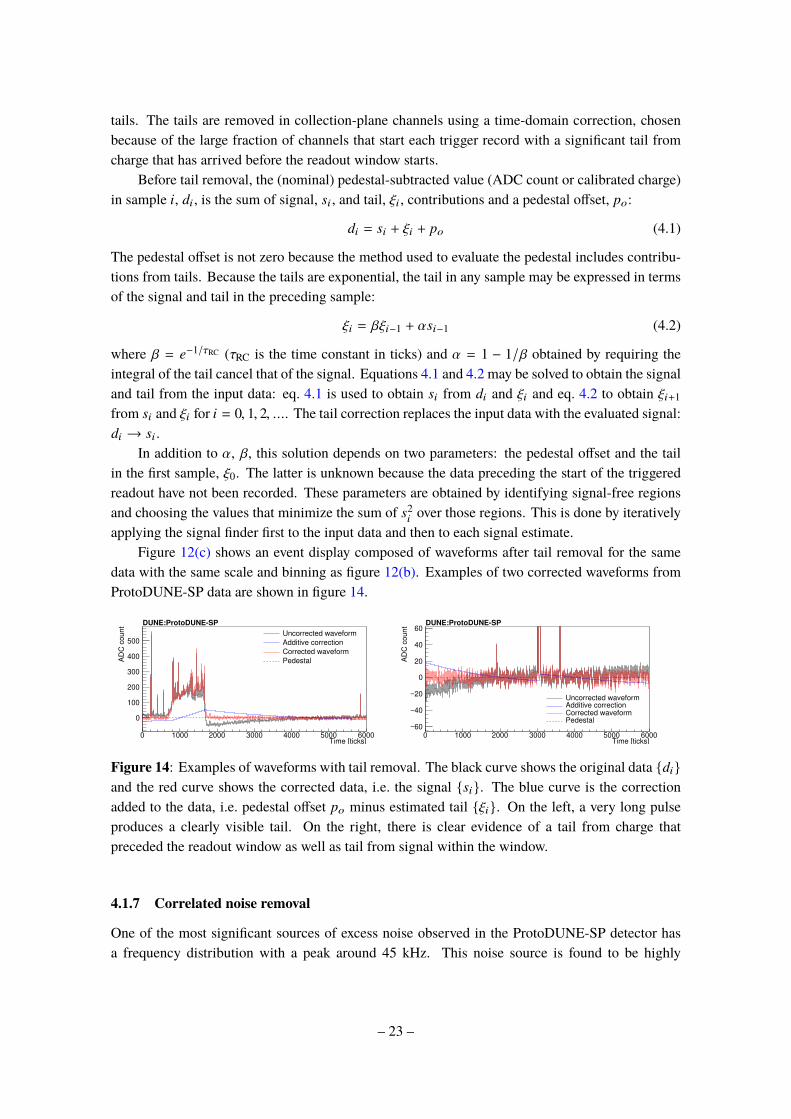
tails. The tails are removed in collection-plane channels using a time-domain correction, chosen

because of the large fraction of channels that start each trigger record with a significant tail from

charge that has arrived before the readout window starts.

Before tail removal, the (nominal) pedestal-subtracted value (ADC count or calibrated charge)

in sample i, di, is the sum of signal, si, and tail, ξi, contributions and a pedestal offset, po:

di = si + ξi + po (4.1)

The pedestal offset is not zero because the method used to evaluate the pedestal includes contribu-

tions from tails. Because the tails are exponential, the tail in any sample may be expressed in terms

of the signal and tail in the preceding sample:

ξi = βξi−1 + αsi−1 (4.2)

where β = e−1/τRC (τRC is the time constant in ticks) and α = 1 − 1/β obtained by requiring the

integral of the tail cancel that of the signal. Equations 4.1 and 4.2 may be solved to obtain the signal

and tail from the input data: eq. 4.1 is used to obtain si from di and ξi and eq. 4.2 to obtain ξi+1

from si and ξi for i = 0, 1, 2, .... The tail correction replaces the input data with the evaluated signal:

di → si.

In addition to α, β, this solution depends on two parameters: the pedestal offset and the tail

in the first sample, ξ0. The latter is unknown because the data preceding the start of the triggered

readout have not been recorded. These parameters are obtained by identifying signal-free regions

and choosing the values that minimize the sum of s2i

over those regions. This is done by iteratively

applying the signal finder first to the input data and then to each signal estimate.

Figure 12(c) shows an event display composed of waveforms after tail removal for the same

data with the same scale and binning as figure 12(b). Examples of two corrected waveforms from

ProtoDUNE-SP data are shown in figure 14.

0 1000 2000 3000 4000 5000 6000Time [ticks]

0

100

200

300

400

500

AD

C c

ou

nt

Uncorrected waveform

Additive correction

Corrected waveform

Pedestal

DUNE:ProtoDUNE-SP

0 1000 2000 3000 4000 5000 6000Time [ticks]

60−

40−

20−

0

20

40

60

AD

C c

ou

nt

Uncorrected waveformAdditive correctionCorrected waveformPedestal

DUNE:ProtoDUNE-SP

Figure 14: Examples of waveforms with tail removal. The black curve shows the original data diand the red curve shows the corrected data, i.e. the signal si. The blue curve is the correction

added to the data, i.e. pedestal offset po minus estimated tail ξi. On the left, a very long pulse

produces a clearly visible tail. On the right, there is clear evidence of a tail from charge that

preceded the readout window as well as tail from signal within the window.

4.1.7 Correlated noise removal

One of the most significant sources of excess noise observed in the ProtoDUNE-SP detector has

a frequency distribution with a peak around 45 kHz. This noise source is found to be highly

– 23 –

correlated among a group of channels that share the same low-voltage regulator in the same FEMB.

Following Ref. [37], a mitigation method is developed by dividing channels into groups. Each

FEMB amplifies and digitizes 128 channels: 40 adjacent U-plane channels, 40 adjacent V-plane

channels, and 48 adjacent collection-plane channels. The U-plane channels form a group, as do

the V-plane channels and the collection-plane channels. For each of the three groups, a correction

waveform is constructed based on the median value of samples from the group at every time tick and

it is subtracted from each channel’s waveform in that group. However, if the majority of waveforms

contain signals of ionization electrons, it is necessary to protect this time region to avoid signal

suppression. A region of interest (ROI) is defined as the ADC counts above an expected threshold

as well as 8 (20) ticks before (after). As an example, event displays consisting of waveforms before

and after the correlated noise removal (CNR) are shown in figure 12(c) and 12(d), respectively.

The correlated noise is visible as vertical bands in figure 12(c), and it is suppressed in figure 12(d).

Some sources of correlated noise remain in some portions of the detector, specifically those for

which the spatial correlation does not coincide with FEMB boundaries.

4.2 Charge calibration

The ProtoDUNE-SP electronics provide the capability to inject a known charge in short-duration

(< 1µs) pulses into each of the amplifiers connected to the TPC wires. The level of that charge is

controlled by a six-bit voltage digital-to-analog converter (DAC) and is nearly linear with Q = SQs

where S is the DAC setting (0, 1, ..., 63) and the step charge Qs = 3.43 fC = 21.4 ke, which is

comparable to the charge deposition of a minimum ionizing particle traveling parallel to the wire

plane and perpendicular to that plane’s wire direction.

A charge calibration is carried out so that ADC counts read out for each channel may be

converted to collected charge. The calibration is expressed as a gain for each channel normalized

such that the product of the gain and the integral of the ADC signal over the pulse in a collection

channel gives the charge in the pulse, i.e. Q = gA. The evaluation of charge for the bipolar TPC

signals in induction channels is more complicated but also proportional to the gain derived here.

Special runs were taken with injected voltage regularly alternating between ground and the

DAC level (one setting for each run) producing charge pulses of alternating sign. Fifty trigger

records with typically 12 pulses of each sign are processed for each channel at each DAC setting.

For each channel, the pedestal is evaluated for each event and a distribution of approximately 600

pedestal-subtracted areas in units of (ADC count)-ticks is obtained for each charge sign. The mean

of these signal area measurements are plotted as a function of DAC setting using data from many

runs, and a line constrained to pass through the origin is fit to DAC settings 1-7. The step charge

divided by the slope of this line provides the calibrated gain for each channel.

Figure 15 shows the uncalibrated area vs. DAC setting and the fit for a typical collection

channel. The response is fairly linear over the DAC setting range (-5, 20) with saturation setting

in outside this range. Typical track charge deposits are one to four times the step charge and

this saturation is only an issue for very heavily ionizing tracks. The gain for this channel is

g = (21.4 ke)/(909.4 (ADC count)-tick) = 23.5 e/((ADC count)-tick).

Figure 16 shows the residuals for the same data, i.e. the measured area minus that expected for

the fitted gain ∆A = A− SQs/g. These results are typical—most of the measured areas for positive

– 24 –

30− 20− 10− 0 10 20 30

Pulser DAC setting

10000−

5000−

0

5000

10000

15000

20000

25000tick]

×A

rea [(A

DC

count)

0.14±Slope: 909.41

DUNE:ProtoDUNE-SP

Figure 15: Measured pulse area vs. DAC setting for a typical collection channel. The red line

shows the fit used to extract the gain.

smaller (S ≤ 7,Q . 160 ke) pulses are within 1% of their fitted values. The systematic shift for

higher values is also typical and presumably reflects non-linearity in the DAC.

All 15,360 ProtoDUNE channels were calibrated in this manner, and those gains are applied

early (before the mitigation and noise removal) in the typical processing of data from the detector.

Figure 17 shows the distribution of these gains for all channels. Channels flagged as bad or

especially noisy in an independent hand scan are shown separately. The gains for the remaining

good channels are contained in a narrow peak with an RMS of 5.1% reflecting channel-to-channel

response variation in the ADCs and gain and shaping time variations in the amplifiers.

4.3 TPC noise level

One very important goal for ProtoDUNE-SP is to demonstrate that noise levels are well below

signals from charged tracks; this is found to be the case for nearly all of the channels in the detector.

The noise is evaluated both for single ADC samples (sample noise) and for a contiguous range of

50 samples (integrated noise). The latter range is chosen to be sufficient to obtain the area of the

signal from a charged track in the detector traveling in the yz plane. Tracks with other angles with

respect to the electric field will leave longer pulses on the sense wires.

The noise is measured after initial data preparation. As discussed in section 4.1, the pedestal

is evaluated for each trigger record, and the charge calibration is applied to the ADC count minus

pedestal to obtain the initial charge measurement for each channel. Sticky codes are mitigated and

the AC-coupling tails are removed in the collection channels. The noise is evaluated both at this

– 25 –

30− 20− 10− 0 10 20 30

Pulser DAC setting

300−

200−

100−

0

100

200

300tick]

×A

rea [(A

DC

count)

∆

DUNE:ProtoDUNE-SP

Figure 16: Measurement residuals (data - fit) for the same data as the preceding figure (black) plus

the same for data taken in the following months (colors). The dashed lines indicate deviations of

±1%.

point and after applying the CNR. The noise is expressed in units of collected electrons. To set

the scale, the bulk of the observed distribution of signal areas in each of the channels starts (as

expected) at about 30 ke.

The high rate of cosmic-ray signals—an average of one every 1500 ticks (0.75 ms) for the TPC-

side collection-plane channels—complicates the measurement of the noise. To avoid contamination

from these and radioactive (e.g. 39Ar) signals, a signal finder is applied and the noise is defined to be

the RMS ADC value outside the signal regions. For the integrated noise measurement, integration

regions start every 50 ticks (i.e. at ticks 0, 50, 100, ...) and regions are discarded if they have any

overlap with signal regions.

The signal finder used for this study makes use of a variable sample threshold and retains a

region of (-30, +50) ticks around any tick with signal magnitude above that threshold. The threshold

is evaluated independently for each channel every trigger record. The threshold starts at 300 e and,

if it is below five times the sample noise, is increased until it reaches that level. This allows efficient

removal of signals in quiet channels while retaining the noise in those that are noisier.

Visual inspection of raw waveforms were performed to identify bad channels in the detector,

mostly those with no signal or exceptionally high noise typically from sticky ADC codes. The

number of such channels is 90, i.e. 0.6% of the channels in the detector. These are excluded from

the noise summary plots below.

Figure 18 shows the distributions of sample and integrated noise levels before and after corre-

lated noise removal for trigger records 1-1000 of run 5240 taken October 12, 2018. The collection-

– 26 –

0.015 0.02 0.025 0.03 0.035

Gain [ke/(ADC count)/tick]

0

200

400

600

800

1000

1200

Nu

mb

er

of

ch

an

ne

ls

Good: count: 15227

mean: 0.0234

RMS/mean: 0.051

Bad: count: 133

DUNE:ProtoDUNE-SP

Figure 17: Distribution of fitted gains for good (blue) and bad/noisy (red) channels. The legend

indicates the number of channels in each category and gives the mean (23.4 e/(ADC count)/tick))

and RMS/mean (5.1%) for the good channels.

plane and induction-plane channels are shown separately and, as expected, the noise levels are higher

for the induction-plane channels as the wires are longer. For the collection channels, the sample

noise is around 100 e before correlated noise removal falling to 80 e after the channel correlations

are removed. The corresponding values for the integrated noise are 1200 e and 900 e.

For charge deposits much faster than the nominal 2 µs shaping time of the amplifier, the area

A of the resulting signal pulse is proportional to the height h and shaping time τ: A = Khτ. The

shape is well understood [37] and has been verified with fits of the ProtoDUNE-SP pulser signals.

Numerical integration gives K = 1.269/tick = 2.538/µs. For such fast signals, the charge may

be deduced directly from the pulse height and its standard deviation is called the ENC (equivalent

noise charge) [37]. The ProtoDUNE-SP signals are slower than this but the ENC is a standard

metric and is presented here to allow comparison with results from other detectors.

The ratio of ENC to sample noise defined here is A/h = Kτ. The actual shaping time varies

from channel to channel but has central value around 2.2 µs which gives a ratio of ENC to sample

noise of 5.58. With this factor and the above values for the sampling noise, the mean ENC for the

collection channels is 530 e before correlated noise removal and 430 e after. The corresponding

numbers for the induction channels are 620 e and 500 e. These noise values are similar to the 500-

600 e values obtained from bench measurements with a prototype FEMB at LN2 temperature [3].

Figure 19 shows the noise frequency power spectra for data collected at the same time as

those used for figure 18. For each channel, a signal finder with a dynamic threshold of five times

the sample RMS in the non-signal region is used to identify signal samples. A discrete Fourier

– 27 –

0 0.05 0.1 0.15 0.2 0.25 0.3 0.35

Noise [ke/tick]

0

200

400

600

800

1000

1200

1400

1600

1800

2000N

um

ber

of channels

DUNE:ProtoDUNE-SP

Sample noise w/o CNR

Run 5240

= 94 e⟩σ⟨Collection:

= 111 e⟩σ⟨Induction:

0 0.5 1 1.5 2 2.5 3 3.5 4 4.5 5

Noise [ke/(50 tick)]

0

200

400

600

800

1000

Num

ber

of channels

DUNE:ProtoDUNE-SP

Integrated noise w/o CNR

Run 5240

= 1216 e⟩σ⟨Collection:

= 1664 e⟩σ⟨Induction:

0 0.05 0.1 0.15 0.2 0.25 0.3 0.35

Noise [ke/tick]

0

500

1000

1500

2000

2500

3000

Num

ber

of channels

DUNE:ProtoDUNE-SP

Sample noise with CNR

Run 5240

= 82 e⟩σ⟨Collection:

= 92 e⟩σ⟨Induction:

0 0.5 1 1.5 2 2.5 3 3.5 4 4.5 5

Noise [ke/(50 tick)]

0

500

1000

1500

2000

2500

Num

ber

of channels

DUNE:ProtoDUNE-SP

Integrated noise with CNR

Run 5240

= 889 e⟩σ⟨Collection:

= 1057 e⟩σ⟨Induction:

Figure 18: TPC sample (left) and 50-sample integrated (right) noise distributions before (top)

and after (bottom) correlated noise removal. Each plot has one entry for each channel excluding

bad channels with overflows shown in the last bin. Collection and induction channels are shown

separately.

transform is performed on non-overlapping blocks of 1000 contiguous samples selected from the

non-signal regions. The power spectra for good channels are averaged separately for each of the

four wire types: TPC-side collection, cryostat-sided collection and the two induction orientations,

U and V. These are normalized so that the sum over power terms or histogram entries is equal to

the RMS charge per sample, i.e. the sample noise shown on the left side of figure 18.

As expected for effective removal of signals from the TPC, the power distributions are very

similar for the TPC-side and cryostat-side collection channels. The induction wire distributions

have similar shapes. The small spike around 300 kHz is due to pickup noise in one of the APAs.

The CNR effectively suppresses both that and the excess noise below 100 kHz.

4.4 Signal processing

The recorded waveform on each TPC readout channel is a linear transformation of the current on

the connected wire as a function of time. This transformation includes the effect of induced currents

due to drifting and collecting charge, as well as the response of the front-end electronics. The goal

of the signal-processing stage of the offline data processing chain is to produce distributions of

charge arrival times and positions given the input waveforms. These charge arrival distributions are

– 28 –

0 200 400 600 800 1000

Frequency [kHz]

0

500

1000

1500

2000

/(20 k

Hz)]

2P

ow

er/

tick/c

hannel [e

= 93 eΣW/o CNR:

= 82 eΣWith CNR:

DUNE:ProtoDUNE-SP

C wires

Run 5240

0 200 400 600 800 1000

Frequency [kHz]

0

500

1000

1500

2000

/(20 k

Hz)]

2P

ow

er/

tick/c

hannel [e

= 111 eΣW/o CNR:

= 92 eΣWith CNR:

DUNE:ProtoDUNE-SP

U wires

Run 5240

0 200 400 600 800 1000

Frequency [kHz]

0

500

1000

1500

2000

/(20 k

Hz)]

2P

ow

er/

tick/c

hannel [e

= 97 eΣW/o CNR:

= 83 eΣWith CNR:

DUNE:ProtoDUNE-SP

Z wires

Run 5240

0 200 400 600 800 1000

Frequency [kHz]

0

500

1000

1500

2000

/(20 k

Hz)]

2P

ow

er/

tick/c

hannel [e

= 113 eΣW/o CNR:

= 94 eΣWith CNR:

DUNE:ProtoDUNE-SP

V wires

Run 5240

Figure 19: Noise frequency power spectra before and after CNR. Each plot is evaluated from

1000-sample blocks in non-signal regions. Upper and lower left respectively show the cryostat- and

TPC-side collection planes. The induction planes are on the right: top is U and and bottom is V.

The first bin in each plot includes only the zero frequency component. The others are sums over

20 kHz bins.

used in subsequent reconstruction steps, such as hit finding. Because the response is linear in the

arriving charge distribution, a deconvolution technique forms the core of the signal processing.

A charge moving in the vicinity of an electrode can induce electric current. Shockley-Ramo’s

theorem [38] states that the instantaneous electric current i on a particular electrode (wire) which

is held at constant voltage, is given by

i = e∇φ · ®ve, (4.3)

where e is the charge in motion, and ®ve is the charge velocity at a given location. The so-called

weighting potential φ of a selected electrode at a given location is determined by virtually removing

the charge and setting the potential of the selected electrode to unity while grounding all other

conductors.

The field response is defined to be the induced current on different wires due to a moving

point charge. The field response is an essential input to the signal processing procedure as will be

discussed below. For ProtoDUNE-SP, the field response is calculated with Garfield [39], a TPC drift

simulation code, in a 2D scheme as illustrated in figure 20(a). During the field response simulation,

a point charge is positioned at different positions in a horizontal plane 10 cm away from the grid

– 29 –

plane and the drift path is recorded from the simulation as shown in figure 20(b). The electron

drift velocity can be determined from the electric field [40, 41], while the precomputed weighting

potential for a U-plane wire is also shown in figure 20(b). With the drift path and the weighting

potential, the field response of the point charge on the sense wire can be calculated according to

eq. (4.3). This procedure is repeated for a series of point charges that spans a region of 21 wires with

the wire of interest at the center. In order to sample the rapidly-changing field response functions

adequately, point charges are simulated drifting in from positions on a grid with a spacing of one

tenth of the wire pitch. After convolving the electronics response, the total response as a function

of time and wire pitch is presented in figure 21, where a “Log10” color scale is defined for the sake

of visibility:

i in “Log10” =

log10(i · 105), if i > 1 × 10−5,

0, if − 1 × 10−5 ≤ i ≤ 1 × 10−5,

−log10(−1 · i · 105), if i < −1 × 10−5.

(4.4)

As shown in figure 20(b), the weighting potential of the first induction (U) plane is significantly

different from zero over a region of a few wires even with the presence of the grid plane. As a result,

the current induced on a sense wire contains contributions not only from charges passing between

the wire and its immediate neighbors, but also from moving charges that are farther away. A region

that is 10 cm in front of the grid plane and ±10 wires around the wire of interest in the simulation

is sufficient to envelope the field response.

In order to deconvolve the ionization electron distribution from the measured signal, it is natural

to mathematically describe this long-range effect as follows:

M(wi1, tj1) =∫

wi2

∫

tj2

∫

tj3

Q(wi2, tj2) · F(wi2 − wi1, tj3 − tj2) · E(tj1 − tj3) · dtj3 · dtj2 · dtwi2

=

∫

wi2

∫

tj2

Q(wi2, tj2) · R(wi2 − wi1, tj1 − tj2) · dtj2 · dtwi2

(4.5)

where measured signal M(wi1, tj1) on the wi1th wire and time tj1 is a convolution of i) the ionization

charge distribution as a function of the position in wire number and the drift time: Q(wi2, tj2), ii)

the field response that describes the induced current on the wires when the ionization charge

move: F(wi2 − wi1, tj3 − tj2), and iii) the electronics response that amplify and shape the induced

current on the wire: E(tj1 − tj3). For simplicity, one can firstly convolve the field response and

the electronics response into the overall response function: R(wi2 − wi1, tj1 − tj2), in which the

fine-grained position-dependent field response function is averaged within one wire pitch.

Because of the long-range induction effect, instead of a 1D deconvolution involving only the

time dimension, a two-dimensional (2D) deconvolution involving both the time and wire dimensions

is performed to extract the ionization electron distribution. In practice, the FFT algorithm is

used to convert the data from the discrete 2D time and wire domain to a discrete 2D frequency

domain [42, 43]. To avoid amplifying high-frequency noise in the deconvolution, two Wiener-

inspired filters are applied separately in both dimensions. In addition, to further reduce the noise

contamination and improve the charge resolution, a technique for identifying the signal regions

of interest (SROI) is adopted and adjusted accordingly. The application of SROIs are particularly

– 30 –

M 0 V

(a)

x [c

m]

z [cm]

(b)

Figure 20: (a) Illustration of the 2D ProtoDUNE-SP TPC scheme for the Garfield simulation,

where ±10 wires (large black dots) are considered for each wire plane and the electrons drift

simulation starts 10 cm away from the grid plane. The inset shows the spacing of the starting points

of the simulated electrons; (b) Garfield simulation of electron drift paths (yellow lines) in a 2D

ProtoDUNE-SP TPC scheme and the equal weighting potential lines (green) for a given wire in

the first induction plane, where the latter is shown in percentage from 1% to 45%. A long-range

induction effect is noticed as the weighting potential has significant strength several wire spacings

away from any particular wire.

important to process the induction plane signals. As an example, a raw waveform that has been

de-noised as described in section 4.1 and the corresponding extracted charge distribution after the

deconvolution are shown in figure 22(a) and figure 22(b), respectively.

4.5 Event Reconstruction

There are two distinct steps in the ProtoDUNE-SP event reconstruction chain to go from the

deconvolved waveforms to fully reconstructed interactions: hit finding and pattern recognition.

These steps are described in sections 4.5.1 and 4.5.2, respectively.

4.5.1 Hit finding

The hit finding algorithm fits peaks in the wire waveforms, where a hit represents a charge deposition

on a single wire at a given time. Each hit corresponds to a fitted peak. Ideally, after the deconvolution

process described in section 4.4, the signals on all wires, regardless of whether they are induction-

plane wires or collection-plane wires, will be waveforms containing possibly overlapping Gaussian-

shaped peaks. The algorithm searches for candidate hits in the waveform and fits them to a

Gaussian shape to produce the hits. Situations can occur in which charge deposits do not form

a simple Gaussian shape, for example when a particle trajectory is close to being in the plane

– 31 –

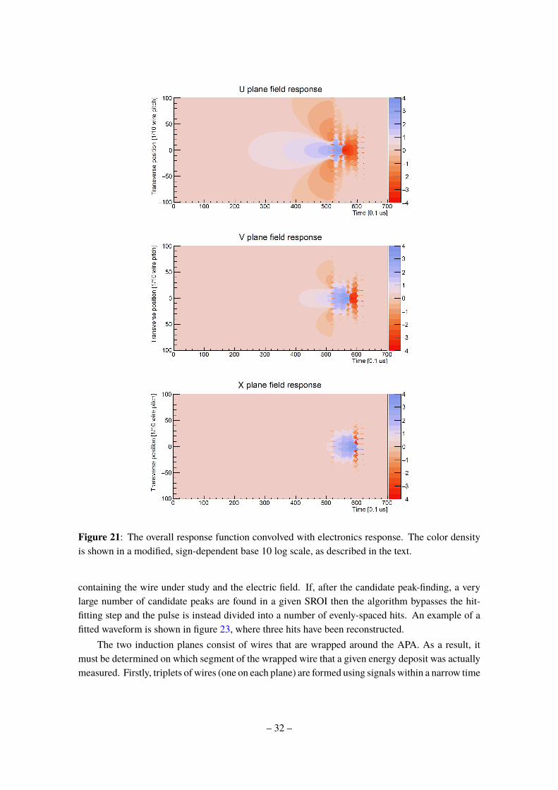
X

Figure 21: The overall response function convolved with electronics response. The color density

is shown in a modified, sign-dependent base 10 log scale, as described in the text.

containing the wire under study and the electric field. If, after the candidate peak-finding, a very

large number of candidate peaks are found in a given SROI then the algorithm bypasses the hit-

fitting step and the pulse is instead divided into a number of evenly-spaced hits. An example of a

fitted waveform is shown in figure 23, where three hits have been reconstructed.

The two induction planes consist of wires that are wrapped around the APA. As a result, it

must be determined on which segment of the wrapped wire that a given energy deposit was actually

measured. Firstly, triplets of wires (one on each plane) are formed using signals within a narrow time

– 32 –

0 25 50 75 100 125 150 175 200U Wire No.

0

100

200

300

400

500

600

Tim

e [

s]

15

10

5

0

5

10

15DUNE:ProtoDUNE-SP

(a) After Noise Filtering

0 25 50 75 100 125 150 175 200U Wire No.

0

100

200

300

400

500

600

Tim

e [

s]

300

200

100

0

100

200

300DUNE:ProtoDUNE-SP

(b) After Deconvolution

Figure 22: An interaction vertex from the 7-GeV charged particle beam data (run 5152, event

89) measured on the induction U plane: (a) Raw waveform in ADC counts after noise filtering;

(b) Ionization charge in number of electrons, scaled by 200, extracted with the 2D deconvolution

technique.

4600 4650 4700s]µTime Tick [0.5

0

10

20

30

40

50

Charg

e/tic

k [200 e

]

Deconvolved waveform

Fitted Gaussian hits

DUNE:ProtoDUNE-SP

Figure 23: An example of a reconstructed waveform on a single wire from ProtoDUNE-SP data.

window. Often, for a given collection wire, only a single pair of induction wires are matched, thus

the hits are disambiguated at this stage. Otherwise, there can be multiple induction wires consistent

in time with the collection wire. In this case, the algorithm aims to minimise the difference in

charge between the collection wire and the candidate induction wires in a deterministic manner.

A full description of the method is given in Ref. [6]. Simulation studies show that this technique

assigns more than 99% of hits to their correct wire segments.

4.5.2 Pattern recognition with Pandora

Pattern recognition in ProtoDUNE-SP is performed using the Pandora software package [44], which

executes multiple algorithms to build up the overall picture of interactions in the detector. Pandora

has been used successfully in other liquid argon time projection chambers (LArTPCs) such as

MicroBooNE [45]. New features have been developed for ProtoDUNE-SP since it differs from

– 33 –

MicroBooNE with its multiple TPCs and drift volumes in addition to the need for a testbeam

particle specific reconstruction chain.

Pandora contains chains of reconstruction algorithms that focus on specific topologies, but they

all follow a common pattern. The first step involves two-dimensional clustering of the reconstructed

hits in each of the three detector readout planes separately. Dedicated algorithms then match sets

of 2D clusters between the three views. If matching ambiguities are discovered, information from

all three views is used in order to motivate changes to the original 2D clustering. Once consistent

matches between 2D clusters have been made, three-dimensional hits are constructed and particle

interaction hierarchies are created.

In the Pandora ProtoDUNE-SP reconstruction, all of the clusters are reconstructed first under

the cosmic-ray hypothesis using a set of algorithms designed to reconstruct track-like particles.

Cosmic-ray candidates are subsequently identified and removed so that beam-particle analysis can

proceed. One important feature of the cosmic-ray reconstruction step is the “stitching” of tracks

across the boundaries between neighboring drift volumes bounded by a CPA or an APA. The

stitching procedure is applied when two 3D clusters have been reconstructed in neighbouring drift

volumes that have consistent direction vectors and an equal but opposite shift in the drift direction

from the CPA or APA. When the clusters are shifted by this amount, a single collinear cluster

with a known absolute position along the drift direction and time t0 relative to the trigger time

is produced. Figure 24 shows the reconstructed t0 distribution for data and simulation for those

cosmic-ray muon tracks that have been stitched at the cathode or anode. Cosmic-ray muons that

cross the cathode have t0 values between -2500 µs and 500 µs, and those that cross the anode have

−250 µs < t0 < 2750 µs. Tracks satisfying one or more of the following criteria are identified as

“clear” cosmic-ray candidates:

• The particle enters through the top of the detector and exits through the bottom.

• The measured t0 for stitched tracks is inconsistent with a particle coming from the beam.

• Any of the reconstructed hits appear to be located outside of the detector when assuming

t0 = 0, which indicates that the object is inconsistent with the timing of the beam.

The hits from these clear cosmic-ray candidates are removed from the trigger record before the

Pandora reconstruction chain continues to further process the data. These tracks, and in particular

those with a measured t0, form a critical component of the various detector calibrations detailed in

section 6.

Once the energy deposits from the clear cosmic rays have been removed, the reconstruction

continues with a 3D slicing algorithm that divides the detector into spatial regions containing all of

the hits from a single parent particle interaction. These 3D slices could contain beam particles or

cosmic rays that were not clear enough to be removed in the first-pass cosmic-ray removal process.

Two parallel reconstruction chains are applied to these slices - one is the aforementioned cosmic-ray

reconstruction, and the other is a test-beam specific reconstruction.

The test-beam specific reconstruction consists of a more complex chain of algorithms capable

of reconstructing the intricate hierarchies of particles seen in hadronic interactions that can produce

numerous track-like and shower-like topologies. Included in this reconstruction chain is a dedicated

– 34 –

3000− 2000− 1000− 0 1000 2000 3000

s]µ [0Reconstructed t

0.00

0.01

0.02

0.03

0.04

0.05

Fra

ctio

n o

f e

ve

nts

Simulation

Data

DUNE:ProtoDUNE-SP

Figure 24: The Pandora reconstructed t0 distribution for cosmic-ray muons that cross either the

cathode or anode in data (black points) and simulation (red).

search for the primary interaction vertex of the test-beam particle. As well as being used to inform

the clustering, the vertex is essential for constructing the correct particle hierarchy.

Once the slices have been reconstructed under both hypotheses, cosmic-ray and test-beam, a

boosted decision tree (BDT) algorithm is used to determine which, if any, of the slices are consistent

with being of test-beam origin. The input variables to the BDT primarily use topological information

to measure the consistency of the interaction with the test-beam particle hypothesis. The output

from the reconstruction is in the form of a particle hierarchy, where links are made between parent

and child particles to give the flow of an interaction from the initial beam particle. Figure 25

shows an example of a fully reconstructed particle hierarchy for a simulated beam interaction,

where the incoming beam π+ is shown as the magenta track. A suite of tools have been produced

for ProtoDUNE-SP analysers to easily access this hierarchical information in order to perform the

analyses.

The charge deposition per unit length, dQ/dx is reconstructed for track-like objects such as

muons, charged pions, kaons, protons and the beginnings of electromagnetic showers. The charge

Q is taken as the area of the Gaussian fit to the individual hit. The segment length dx is calculated

as the wire spacing divided by the cosine of the angle between the track direction and the direction

normal to the wire direction in the wire plane. The raw dQ/dx is further calibrated to remove

nonuniform detector effects and converted to energy loss dE/dx for energy measurement and

particle identification. This procedure is described in section 6.3.

4.6 Signal to noise performance

The measurement of the signal-to-noise ratio (S/N) for the ProtoDUNE-SP detector is carried out

using a selected cosmic-ray muon sample in Run 5432 taken on Oct. 20, 2018. Muon tracks crossing

– 35 –

Beam π+

<latexit sha1_base64="lrM6zOIadMZqc/YrGNuhJjWYmMo=">AAAB/HicbVDLSsNAFJ3UV62vaJduBosgCCWpgi5L3bisYB/QxDKZTtqhkwczN2II7a+4caGIWz/EnX/jtM1CWw8MHM65h3vneLHgCizr2yisrW9sbhW3Szu7e/sH5uFRW0WJpKxFIxHJrkcUEzxkLeAgWDeWjASeYB1vfDPzO49MKh6F95DGzA3IMOQ+pwS01DfLDrAnkEHW0KHJ1In5w3nfrFhVaw68SuycVFCOZt/8cgYRTQIWAhVEqZ5txeBmRAKngk1KTqJYTOiYDFlP05AETLnZ/PgJPtXKAPuR1C8EPFd/JzISKJUGnp4MCIzUsjcT//N6CfjXbsbDOAEW0sUiPxEYIjxrAg+4ZBREqgmhkutbMR0RSSjovkq6BHv5y6ukXavaF9Xa3WWl3sjrKKJjdILOkI2uUB3doiZqIYpS9Ixe0ZsxNV6Md+NjMVow8kwZ/YHx+QMnmpUW</latexit>

Figure 25: A reconstructed, simulated test-beam interaction showing the incoming beam π+ track

in magenta and a number of secondary particles created at the interaction vertex. The different

colors represent different reconstructed particles.

the LArTPC at shallow angles with respect to the anode plane and large angles with respect to the

direction of the wires in the planes are considered for the S/N characterization. To ensure good

track quality, track length is required to be at least 1 m. The electron drift lifetime of the sample

was approximately 24 ms as independently measured by the purity monitor.

The signal on each wire in a plane is defined to be the maximum pulse height of the raw

waveform after subtracting the pedestal. The noise value is defined to be the standard deviation

of a Gaussian function fit to the distribution of ADC values in signal-free regions of a channel’s

waveform. The signal size depends on the angle of the track with respect to the wire and also with

respect to the electric field. We standardize the signal on a wire to be that from tracks that are

perpendicular to the wire and also perpendicular to the electric field. We define two angles θxz (the

angle made by the projection of a track on the xz plane with the z direction) and θyz (the angle made

by the projection of a track on the yz plane with the z direction). The two angles are illustrated in

figure 26. To minimize the influence of angular dependence of S/N, we select muon tracks that have

minimum component in both drift and wire direction. Angle cuts of θxz and θyz within 20 are

applied. A correction is applied to the raw waveform signal to standardize the strength, adjusting

for angular effects.

The angle-corrected S/N distributions are shown in figure 27. No electron drift lifetime

corrections are applied to the angle-corrected S/N calculations. The most probable values (MPVs)

of the S/N distributions after the noise mitigation are 40.3, 15.1, and 18.6 for the collection plane,

the U plane, and the V plane, respectively. The actual performance of the S/N for the three planes

is much better than the expectation in the ProtoDUNE-SP technical design report [3] - 9.0 for the

three planes. The angle-corrected S/N results with and without the noise filters, together with the

– 36 –

y

z

x

θxz

θyz

Track D

irectio

n

Figure 26: The definitions of the track direction angles θxz and θyz

estimation using the averaged values of the S/N distributions, are summarized in table 2.

The differences in the average S/N values for the three planes is explained using the Shockley-

Ramo theorem, discussed in section 4.4. The three planes have similar weighting fields but different

local drift velocities. Among the three planes, the collection plane has the largest local drift velocity

and hence the best S/N performance. The S/N performance is slightly better for the V plane with

respect to the U plane. This is because the local drift velocity at the V plane is higher than that of

the U plane due to larger bias voltage, while the weighting fields are the same for both.

Table 2: Summary table of the angle-corrected S/N performance before and after the noise mit-

igation for the ProtoDUNE-SP detector. No electron drift lifetime corrections are applied. The

most-probable value (MPV) and the average value for each plane are listed.

Plane

Peak signal-to-noise ratio

Raw Data After noise filtering

MPV Average MPV Average

Collection 30.9 38.3 40.3 48.7

U 12.1 15.6 15.1 18.2

V 14.9 18.7 18.6 21.2

5 Photon detector characterization

5.1 The photon detector system

The ProtoDUNE-SP photon detector system (PDS) comprises 60 optical modules embedded within

the six APA frames of the TPC. These modules view the LAr volume from each anode side opposite

the central cathode. Three different photon collection technologies proposed for DUNE’s far

detector modules [3] are implemented in ProtoDUNE-SP’s PD system. In each technology, incident

– 37 –

0 50 100 150Angle-Corrected Signal-to-Noise Ratio

0.0

0.2

0.4

0.6

0.8

1.0

Re

lative

Fre

qu

en

cy

U Plane, Raw

V Plane, Raw

Collection Plane, Raw

U Plane, Noise-filtered

V Plane, Noise-filtered

Collection Plane, Noise-filtered

DUNE:ProtoDUNE-SP Cosmics Data

Figure 27: Angle-corrected S/N distributions before and after the noise filtering of the three planes

using the cosmic-ray muons for the characterization. The histograms are normalized such that the

maximum frequency is one.

LAr scintillation photons, which have wavelengths around 128 nm, are converted into longer-

wavelength photons using photofluorescent compounds as wavelength shifters (WLS). Visible light

is trapped within the modules, a portion of which is eventually incident on an array of silicon

photomultiplier photosensors (SiPMs) [19].

5.1.1 Light collectors

Each APA contains ten support structures located behind the wire planes for the PDS modules.

Each module is a long, thin bar oriented along the z axis. The spacing between modules in y

is approximately 60 cm, as illustrated in figure 28. Of the 60 modules, two are based on the

ARAPUCA photon detector technology [46], 29 are dip-coated light guides [47, 48], and 29 are

double-shift light guides [49]. All light-guide modules have the same dimensions. The optical

area of a module is 207.4 × 8.2 cm2 in size, and the light is read out on one end of the bar. The

ARAPUCA modules are segmented longitudinally (along the z direction) into 12 cells, each with its

own readout. The first eight cells each have an optical area of 9.8× 7.9 cm2 and the remaining four

cells are double-area cells, each with an optical area of 19.6 × 7.9 cm2. One ARAPUCA module

is located in the top half of the upstream APA in the beam-side drift volume. A second is located

in the middle of the APA in the center of the opposite drift volume. The two light-guide designs

fill the remaining modules in alternating positions in the APAs. One example of each module

– 38 –

type is highlighted in figure 28, together with the photo-sensor arrays equipping the module. The

installation of the modules within an APA behind the wire planes and a grounding mesh is also

visible in figure 28.

PD Module Designs

Dip-Coated Light Guides

Double-Shift Light Guides

ARAPUCA (Light Trap)

Figure 28: Picture of a ProtoDUNE-SP APA during assembly. Labels indicate the three types of

PDS modules inserted into the APA frame (left). Pictures of the three technologies (right) with

details of the photo-sensor arrays equipping the modules (insets). From left to right, they are a

dip-coated light-guide module, a double-shift light-guide module, and an ARAPUCA module.

The two light-guide designs convert incident VUV photons into the visible range using tetra-

phenyl butadiene (TPB) (emission peak ∼430 nm), while the ARAPUCA design uses p-terphenyl

(PTP) (emission peak ∼340 nm). In the dip-coated acrylic light guide, wavelength-shifted photons

are confined inside by total internal reflection and they are guided toward the end of the bar that is

in optical contact with a photosensor array. The double-shift light guide contains an internal light

guide doped with the second WLS (490 nm emission) to facilitate trapping of double-converted

photons within the module and guide them toward the photosensors at the end of the bar. The

ARAPUCA uses a dichroic filter window (400 nm cutoff) to reflect photons from a second WLS

(TPB) inside the cell underneath the window and prevent them from exiting before they are absorbed

or detected by the photosensors distributed inside the cell.

5.1.2 Photosensors

Three silicon photosensor models, each with an active area of 6× 6 mm2, are employed throughout

the photon detection system. They were selected among those that were available commercially or

that were newly developed during the PDS material procurement phase: the SensL SiPM MicroFC-

– 39 –

60035-SMT (35 µm pixel size) and two types of Hamamatsu MPPC S13360-6050 (50 µm pixel size)

- the CQ-type (Quartz windowed for Cryogenic application) and the VE-type (VErtical through-

silicon via). Arrays of photosensors of the same model are passively ganged together in parallel

forming large-area single channels for voltage supply and signal readout. The arrays formed by

three SensL SiPMs are indicated in the following as 3-S-SiPM, those formed by 3 Hamamatsu

MPPCs (VE-type) indicated as 3-H-MPPC and those with 12 Hamamatsu MPPC (CQ-type) as

12-H-MPPC. Each of the light-guide modules is read out by four channels with three photosensors

each, either 3-S-SiPM or 3-H-MPPC, arranged in a strip of 12 photosensors in total at one end of

the module. Each cell of each ARAPUCA module is read out by one 12-H-MPPC channel made

of 12 Hamamatsu MPPCs distributed in the plane opposite to the cell optical window, for a total of

144 photosensors in the ARAPUCA module (12 cells). The numbers of channels of the different

types and their distribution in the PDS modules are summarized in table 3. A 12-H-MPPC array

and a strip made by four 3-S-SiPM are shown in figure 28.

Table 3: Numbers of each type of PDS module installed in ProtoDUNE-SP, and the numbers of

sensors per channel and channels per module

Ph. sensors Type Channels Dip-coated Double-shift ARAPUCA Total channels

per channel of channel per module modules modules modules in PDS

3 3-S-SiPM 4 21 22 - 172

3 3-H-MPPC 4 8 7 - 60

12 12-H-MPPC 12 - - 2 24

The ratio of the photosensor area to the light collector surface area for the light-guide modules

(0.26%) is lower than that of the ARAPUCA cells (4.2% and 2.1% for the cells with double area).

5.1.3 Readout DAQ and triggering

Unamplified signals from the photosensors in the LAr are transmitted outside the cryostat on copper

cables. A dedicated, custom module was built for receiving and processing silicon photosensor

signals for the trigger and DAQ. The module is called the SiPM Signal Processor (SSP). A self-

contained, 1U SSP module reads out 12 independent PDS channels. Each channel has a voltage

amplifier and a 14-bit, 150 megasamples per second ADC that digitizes the (current) output signal

from photosensors into analog-to-digital units. The front-end amplifiers are configured to be fully-

differential with high common-mode noise rejection. Each amplifier has on its input a termination

resistor that matches the 100 Ω characteristic impedance of the signal cable. The least-significant

ADC bit corresponds to 66 nA in this configuration. The digitized data are stored in pipelines

in the SSP, corresponding to as much as 13.3 µs per trigger. The processing is performed by

FPGA (Field-Programmable Gate Array). The FPGA implements an independent data processor

for each channel. The processing incorporates a leading-edge discriminator and a constant fraction

discriminator for sub-clock timing resolution. A block diagram of the system is shown in Fig. 29.

Each channel is individually triggerable. Triggers can come from a periodic trigger, an internal

trigger based on the leading-edge discriminator local to the individual channel, or an external

global trigger distributed by the timing system as the general triggers issued by the beam line

– 40 –

Figure 29: Block diagram of the ProtoDUNE-SP photon-detector readout module (SSP) with

interfaces to Trigger and DAQ systems.

instrumentation (sections 3.1,3.3). If a trigger is present, the channel will produce a data packet

consisting of a header and a waveform (a sequence of values in ADU) of predefined length. An

artDAQ process in the PD DAQ system (SSP boardreader) generates a fragment when the timing

system produces a trigger. This fragment contains all packets received from the SSP with timestamps

in a window ±2.5 ms from the timestamp of the trigger. Each SSP fragment contain 12 packets,

one for each channel, with identical timestamps corresponding to the trigger time, and an arbitrary

number of additional packets generated for channels that have discriminators that fired.

5.1.4 Photon detector calibration and monitoring system

The PDS incorporates a pulsed UV-light monitoring and calibration system to determine the

photosensors’ gains, linearities, and timing resolution, and to monitor the stability of the system

response over time.

The system hardware consists of both warm and cold components. Figure 30 (left) shows a

schematic of the ProtoDUNE-SP PD calibration and monitoring system. Diffusers mounted on

the cathode-plane assembly panels serve as point light sources that illuminate the APA with the

PDS modules on the opposite side of the drift volume. The location of the diffusers on the CPA

panel is indicated by magenta discs. Also shown are the quartz fibers from the top of the CPA to

the diffusers. The other CPA side holds a second set of five diffusers to calibrate the PDS in the

opposite APA array.

The active system component is a 1U rack mount Light Calibration Module (LCM) sitting

outside the cryostat. The LCM generates light pulses that propagate through the quartz fiber-

optic cable to the diffusers at the CPA. The LCM consists of an FPGA-based control logic unit

coupled to an internal LED Pulser Module (LPM) and an additional bulk power supply. The LPM

– 41 –

Figure 30: The ProtoDUNE-SP photon-detector calibration and monitoring system installation

on the CPA panels (left). The inset shows the actual lower left diffuser at time of installation.

Waveforms in a LED calibration run displayed in persistence trace mode (right) showing recorded

single and multi-photon signals. Each time tick (tt) represents 6.67 ns.

utilizes multiple digital outputs from the control board to control the pulse characteristics, and it

incorporates DACs to control the LPM pulse amplitude.

The calibration system produces UV light flashes with predefined pulse amplitude, pulse

width, repetition rate, and total number of pulses. A typical photosensor response to low amplitude,

shortest duration calibration pulses is shown in figure 30 (right) where many recorded waveforms

are overlaid with the color indicating the frequency, as in an oscilloscope persistence trace mode.

The UV light flashes can be produced in pairs with a fixed time difference between the two pulses

to study timing properties of the photon system.

5.2 Photosensor performance

Silicon photomultipliers convert light flashes into analog electrical pulses. When a photon hits

and is absorbed in a microcell of the avalanche photodiode matrix, an electron is lifted into the

conduction band. If the bias voltage exceeds the breakdown voltage, this photoelectron creates an

avalanche multiplication, with amplification (gain) typically in the 106 range, which leads to a rising

current signal. Silicon photomultipliers are implemented as photosensors in the ProtoDUNE-SP

PDS modules because of their compact design, low operating voltage and sensitivity to single

photons. To overcome the limitation due to their small sensitive area (6 × 6 mm2) and to limit

the number of channels, arrays of photosensors are passively ganged together in parallel forming

a large-area single channel for voltage supply and signal readout. The capacitance of the array

however increases with the number of photosensors connected in the array, and correspondingly

its recovery time. Therefore, the signal amplitude decreases and the intrinsic noise increases.

Operating at cryogenic temperature helps reduce the dark count rate. On the other hand, correlated

noise — afterpulses in the same pixel and optical crosstalk in neighboring pixels, both generated

– 42 –

by the primary photoelectron event — is expected to grow at high signal gain settings. The adopted

multiplicity of the arrays in the ProtoDUNE-SP PDS design (three per channel in the 3-S-SiPM

and 3-H-MPPC for the electron bars and twelve per channel in the 12-H-MPPC for the ARAPUCA

cells) and the working parameters for operation (bias voltage and gain) were determined with

the requirement of acceptable signal-to-noise ratio allowing for sensitivity to single photoelectron

discrimination with minimal secondary effects.

Fifteen channels out of a total of 256 show anomalous readings. There are two that appear

to be disconnected. They fail their continuity checks and they have been unresponsive since the

earliest tests after cabling. There are two that appear to respond anomalously to light signals. Their

gains are similar to the others, but are somewhat higher, and their peak signal amplitudes are much

higher than those of similar channels. The remaining 11 pass their continuity checks but they do

not respond to light signals. These anomalous channels (all of the 3-S-SiPM type) have not been

investigated further. No channels have changed state since detector operation began.

The photosensor response is characterized using dedicated calibration runs that have fast, low-

amplitude LED flash triggers. Data are collected at several different bias voltage settings. These

calibration runs are periodically repeated in time.

5.2.1 Single photoelectron sensitivity

0 500 1000 1500 2000Time [tt]

10−

0

10

Am

plit

ude [A

DU

]

DUNE:ProtoDUNE-SP 3-S-SiPM

0 500 1000 1500 2000Time [tt]

10−

0

10

Am

plit

ude [A

DU

]

DUNE:ProtoDUNE-SP 12-H-MPPC

Figure 31: Sample waveforms of single photon signal from a 3-S-SiPM channel (left) and 12-H-

MPPC channel (right) (three and twelve sensors passively ganged in parallel, respectively). Noise

filtered waveforms (red histogram) are superimposed, from noise-removal algorithms applied in

data processing.

Signal extraction and noise evaluation are performed for each recorded waveform. The wave-

form consists of 2000 samples of the photosensor output (in ADC units - ADU) at discrete, evenly

spaced points in time ("time ticks" - tt). The sampling interval is 6.67 ns and the duration of the

waveform is 13.3 µs. The trigger time, either from the global trigger or from the SSP internal

trigger, is at a fixed time relative to the start of the waveform. Typical recorded waveforms are

shown in figure 31.

The mean of the pedestal distribution, determined from a pre-sample portion of the waveform

before the trigger, gives the baseline value and the spread (σN ) is an estimate of the noise in the

– 43 –

recorded event. After baseline subtraction, the charge of the signal (in ADU × tt units, proportional

to number of electrons or fC, where 1 ADU × tt = 2750 electrons) is evaluated by integration

of the portion of the waveform starting from the trigger time and extending over a 7 µs (1050

tt) time window. De-noising algorithms that preserve the signal rise time and integral [50] are

applied to more precisely evaluate the maximum amplitude in the same window corresponding to

the photoelectron current of the signal (in ADU or µA).

During detector assembly, the photosensors for each of the three- and twelve-unit channels were

pre-selected based on minimal difference in their nominal breakdown voltage (at warm temperature)

from that listed in data sheets. After this selection, the spread in breakdown voltages among the

sensors in the same 12-H-MPPC channel is typically ∆Vmaxbd

≤ 300 mV. All sensors in a channel

are biased at the same common voltage VB, and the pre-selection thus enables the photosensors in

the channels to all operate in relatively similar working conditions.

Typical charge (signal integral) and current (signal amplitude) distributions under pulsed LED

illumination and with a nominal operating VB setting are shown in figure 32 for a 12-H-MPPC

channel (top row) and for a 3-S-SiPM channel (bottom row).

0 1000 2000 3000 4000 5000 tt]×Charge [ADU

0

200

400

600

800

1000

1200

En

trie

s /

bin

12-H-MPPCDUNE:ProtoDUNE-SP

0 10 20 30 40 50Max Amplitude [ADU]

0

200

400

600

800

1000

En

trie

s /

bin

12-H-MPPCDUNE:ProtoDUNE-SP

0 2 4 6 8 10

310×

tt]×Charge [ADU

0

200

400

600

800

1000

1200

1400

En

trie

s /

bin

3-S-SiPMDUNE:ProtoDUNE-SP

0 20 40 60 80Max Amplitude [ADU]

0

200

400

600

800

1000

En

trie

s /

bin

3-S-SiPMDUNE:ProtoDUNE-SP

Figure 32: Charge (left) and current (right) distribution for typical 12-H-MPPC channel (VB = 48 V)

(top) and 3-S-SiPM channel (VB = 26 V) (bottom) under low amplitude pulsed LED illumination.

A fit of the charge distributions with a multi-Gaussian function giving peak positions and widths is

shown in red.

The multi-peak structure corresponds to detection of 0, 1, 2, . . . photoelectron-induced avalanches.

The clear peak separation confirms good sensitivity to single PE detection for both the three-sensor

– 44 –

and the twelve-sensor channels. The spread around the peaks in the charge spectra (left panels)

is partly due to over-voltage difference among sensors in the array. The asymmetric distribu-

tions around the peaks in the signal amplitude spectra (top right panel) may be due to secondary

avalanches from afterpulses and crosstalk in the sensors more visible in the H-MPPC due to the

faster recharge time. The 1-PE charge directly measures the overall gain of the photosensor array

at the applied bias voltage. The gain gi thus provides the charge per avalanche issued by the i−th

channel.

The gain as a function of bias voltage is shown in figure 33 for some of the 12-H-MPPC

channels and 3-S-SiPM channels. The gain response to varying VB is very uniform channel by

channel, as indicated by the slopes of the lines in figure 33. On the other hand, the intercept with

the horizontal axis, that defines the actual breakdown voltage Vbd of the multi-sensor channel at

LAr temperature, shows a relatively large spread, particularly for the 12-H-MPPC channels.

At the reference bias setting adopted for PDS operation (VB = 48 V for the 12-H-MPPC,

VB = 26 V for the 3-S-SiPM - in either case within the range suggested by the different manufacturers)

the two types of photosensors are operated at different over-voltages VoV = (VB − Vbd) in the range

(3.3 - 4.2) V for the 12-H-MPPC channels and (5.0 - 5.5) V for the 3-S-SiPM channels. Gains are

correspondingly higher, by a factor ∼ 2, for the 3-S-SiPM channels as indicated in figure 33.

44 46 48 50Bias voltage [V]

0

1

2

3

]6

10

× G

ain

[

DUNE:ProtoDUNE-SP 12-H-MPPC

20 22 24 26Bias voltage [V]

0

2

4

6

]6

10

×G

ain

[

DUNE:ProtoDUNE-SP 3-S-SiPM

Figure 33: Gain as a function of applied bias voltage for 12-H-MPPC channels (left), and for

3-S-SiPM channels (right). Linearity of individual channel response is shown by the linear fit

(red line) across the points at different bias voltage setting. The intercept of the fit line provides a

direct evaluation of the breakdown voltage at LAr temperature for each 12-H-MPPC and 3-S-SiPM

photosensor.

5.2.2 Signal to noise in photosensors in passive ganging configurations

The signal-to-noise ratio (SNR) is a good performance metric for the characterization of the

photosensor component of the PDS during normal operating conditions. The SNR of the individual

channel (three or twelve photosensors in parallel) at the reference bias voltage setting is here defined

as:

SNR =µ1

σ0

(5.1)

– 45 –

where, referring for example to figure 32 (left panels), the signal µ1 is the mean value from the

Gaussian fit of the one-PE peak (the minimal detectable signal), and the noise is evaluated from the

Gaussian spread, σ0 of the zero-PE peak. The SNR for all channels of the three types are shown

in figure 34. For the 12-H-MPPC channels of the ARAPUCA modules, the SNR values are around

6, while for the 3-S-SiPM channels of the double-shift and dip-coated bar modules the SNR is in

the range 10 to 12. The signal-to-noise ratio, as defined in equation 5.1, is directly proportional to

the gain and the higher SNR shown by the 3-S-SiPM channels is primarily due to their higher VoV

setting adopted for operation.

0 50 100 150

Channel

0

5

10

15

20

SN

R

DUNE:ProtoDUNE-SP 3-S-SiPM

0 10 20 30 40 50Channel

0

5

10

15

20

SN

R

DUNE:ProtoDUNE-SP 3-H-MPPC

0 5 10 15 20 25Channel

0

5

10

15

20

SN

R

DUNE:ProtoDUNE-SP 12-H-MPPC

Figure 34: Signal-to-Noise Ratio (SNR) for the 3-S-SiPM channels (left), for the 3-H-MPPC

channels (center), and for the 12-H-MPPC channels (right).

5.2.3 Light calibration

Calibration of the light response is necessary to convert the charge signal from the photosensors

into the corresponding number of photons detected. The detector calibration LED pulser is flashed

synchronously with the data acquisition. Calibration runs at varying intensities of the flasher are

needed in order to produce a suitable illumination in each PDS element. For each channel, the

digitized waveform recorded in coincidence with the short LED pulse is baseline subtracted and

the photosensor charge output is measured by waveform integration over a predefined time window

(see section 5.1). Typical charge distributions with multi-peak structure from a LED calibration

run are shown in figure 32 (left panels, top for a 12-H-MPPC channel and bottom for a 3-S-SiPM

channel).

Among the possible different calibration methods, the one adopted here relies on the statistical

features of photon counting measurements under stable pulsed, low illumination conditions. The

number of detected photons (n) per light flash follows the Poisson distribution with λ, the expected

mean number of photons detected per flash, whose value is directly related to the probability of

detecting 0-photons in that flash:

P(n) = λne−λ

n!with P(0) = e−λ → λ = − ln P(0) (5.2)

The probability P(0) can be estimated by the relative frequency of detecting zero photoelectrons in

many LED trials, and from this the mean number of photons detected per flash is inferred:

λ = − ln

(N0

NTot

)(5.3)

– 46 –

where N0 is the observed number of counts under the zero-PE peak (1st peak in the charge distribution

of figure 32 - left panels) and NTot is the number of LED flashes in the calibration run.

The mean number of photons per flash, λ, depends on the illumination level (LED flash

amplitude). The illumination is maintained constant during the run and low enough to have

sufficient probability of 0-photon detected. In addition to this, the measured rate is corrected for the

accidental background rate of environmental photons, which are not correlated to the LED flash,

that may be detected in the trigger window. The background rate is measured in the portion of the

recorded waveforms before the LED trigger.

0 1 2 3 4 5 6 [V]oVV

0

1

2

3

4

5

]6

10

× C

ha

rge

[e

/ ndf 2χ 0.9038 / 5

Prob 0.9699

p0 0.05813±0.01003 − p1 0.01547± 0.5308

/ ndf 2χ 0.9038 / 5

Prob 0.9699

p0 0.05813±0.01003 − p1 0.01547± 0.5308

/ ndf 2χ 0.2771 / 4

Prob 0.9912p0 0.03156± 0.01073 p1 0.5093± 0.8627 p2 0.07006± 0.5335

/ ndf 2χ 0.2771 / 4

Prob 0.9912p0 0.03156± 0.01073 p1 0.5093± 0.8627 p2 0.07006± 0.5335

Gain

Calibration factor

12-H-MPPCDUNE:ProtoDUNE-SP

0 2 4 6 [V]oVV

0

2

4

6

8

]6

10

× C

ha

rge

[e

/ ndf 2χ 0.01447 / 5

Prob 1p0 0.1859±0.00537 − p1 0.0388± 0.8227

/ ndf 2χ 0.01447 / 5

Prob 1p0 0.1859±0.00537 − p1 0.0388± 0.8227

/ ndf 2χ 1.465 / 4Prob 0.8328p0 0.2529± 0.07685 p1 0.3996± 0.5232 p2 0.2684± 0.778

/ ndf 2χ 1.465 / 4Prob 0.8328p0 0.2529± 0.07685 p1 0.3996± 0.5232 p2 0.2684± 0.778

Gain

Calibration factor

3-S-SiPMDUNE:ProtoDUNE-SP

Figure 35: Charge signal per detected photon (blue points) and charge signal per avalanche (black

points) as a function of applied over-voltage VoV for a typical 12-H-MPPC channel (left), and 3-

S-SiPM channel (right). The difference is due to the correlated noise contribution, mainly from

afterpulse and crosstalk in neighboring microcells of the photosensor. The vertical dotted line at

the operation over-voltage set point indicates the gain gi and the calibration factor ci used in data

analysis for the i-th channel shown in the figure.

The photosensor response to λ detected photons, estimated by equation (5.3), is the mean

charge output per flash 〈Q〉 in the calibration run (average of the distribution shown in figure 32

- left panels). The calibration factor for the i-th PDS channel is thus determined by the ratio

ci = 〈Q〉i/λi and represents the output charge per photon detected by the individual photosensor

channel.

The charge issued when an incident photon is detected is expected to be, on average, larger than

the single-avalanche induced charge. The comparison of the charge per photon detected (calibration

factor ci - blue line) and charge per avalanche (gain gi - red line) as a function of the applied over-

voltage VoV is shown in figure 35 for a typical 12-H-MPPC channel (left), and 3-S-SiPM channel

(right). The difference is due to the correlated noise contribution to the signal formation in the

photosensor. This is found to grow exponentially with increasing voltage.

5.2.4 Afterpulses and crosstalk

A common feature of Si-photosensors is the generation of avalanche pulses subsequent to a primary

event. The avalanche of a single microcell in a device has a finite probability of inducing an

– 47 –

avalanche in neighboring microcells (optical crosstalk), or/and of re-triggering itself before the

microcell is fully recovered (afterpulse).

0 50 100 150

Channel

1.0

1.2

1.4

1.6

1.8

2.0

<A

va

lan

ch

e>

/Ph

DUNE:ProtoDUNE-SP 3-S-SiPM

0 10 20 30 40 50Channel

1.0

1.2

1.4

1.6

1.8

2.0

/ P

h⟩

Ava

lan

ch

e

⟨

3-H-MPPCDUNE:ProtoDUNE-SP

0 5 10 15 20 25Channel

1.0

1.2

1.4

1.6

1.8

2.0

/ P

h⟩

Ava

lan

ch

e

⟨

DUNE:ProtoDUNE-SP 12-H-MPPC

Figure 36: Afterpulse and crosstalk contribution to the photosensor signal expressed by the average

number of avalanches generated per detected photon for the 3-S-SiPM channels (left), for the 3-H-

MPPC channels (center), and for the 12-H-MPPC channels (right).

The rate of these secondary pulses increases at higher gain settings. The correlated noise

due to these effects is a well-known limiting factor for a precise photon counting with silicon

photosensors. The measurement of the charge per photon detected (the calibration factor ci, defined

in section 5.2.3) and the charge per avalanche (the gain gi, defined in section 5.2.1) allows the

calculation of the crosstalk and afterpulse probability for each photosensor by the ratio ci/gi in

units of [Ava/Ph], average number of avalanches per photon detected. This ratio is sensitive to

the over-voltage on the photon detector and can be used to monitor for changes in the operating

characteristics of the photosensor as a measure of the stability of the PD system. Figure 36 shows the

measured avalanche/photon value for each channel in the PDS. An average of ∼1.3 Ava/Ph is found

for the 3-S-SiPM channels and the 12-H-MPPC, while a larger factor ∼1.6 Ava/Ph characterizes the

3-H-MPPC channels.

5.2.5 Response stability over time

The sensor gain, the calibration factor and the size of the afterpulse and crosstalk component of the

signal can be used as a system monitor. Any drift in these parameters is an indication of instability

in the system. The calibration data taken at various times during operation provide measurements

that indicate the system stability as a function of time. Figure 37 shows the value of the gain for

typical 12-H-MPPC channels and 3-S-SiPM channels over the course of several months. Within

the uncertainties of the measurements, neither the gain nor the other parameters were found to be

drifting over time for any of the sensors used in the ProtoDUNE-SP photon detector system.

5.3 Photon detector performance

The PD modules (ARAPUCA and light-guide bars) are exposed to scintillation light from ionization

events in the drift volume. A fraction of the emitted photons impinge upon the optical surface of any

given PDS module, and a charge signal is issued, proportional to the number of photons detected

by the photosensors of the module. The detection efficiency ǫD of a PDS module is defined here as

the ratio of detected photons to impinging photons. Test-beam data from particles of known type,

– 48 –

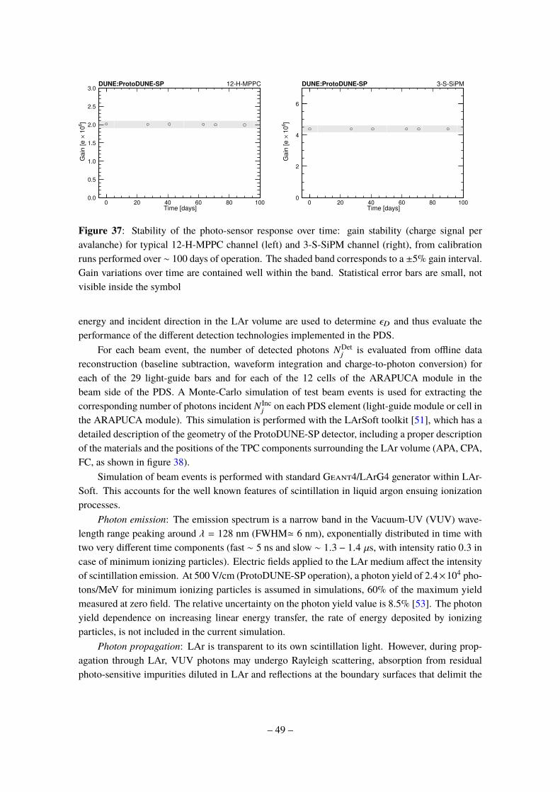
0 20 40 60 80 100 Time [days]

0.0

0.5

1.0

1.5

2.0

2.5

3.0

]6

10

× G

ain

[e

DUNE:ProtoDUNE-SP 12-H-MPPC

0 20 40 60 80 100 Time [days]

0

2

4

6

]6

10

× G

ain

[e

DUNE:ProtoDUNE-SP 3-S-SiPM

Figure 37: Stability of the photo-sensor response over time: gain stability (charge signal per

avalanche) for typical 12-H-MPPC channel (left) and 3-S-SiPM channel (right), from calibration

runs performed over ∼ 100 days of operation. The shaded band corresponds to a ±5% gain interval.

Gain variations over time are contained well within the band. Statistical error bars are small, not

visible inside the symbol

energy and incident direction in the LAr volume are used to determine ǫD and thus evaluate the

performance of the different detection technologies implemented in the PDS.

For each beam event, the number of detected photons NDetj

is evaluated from offline data

reconstruction (baseline subtraction, waveform integration and charge-to-photon conversion) for

each of the 29 light-guide bars and for each of the 12 cells of the ARAPUCA module in the

beam side of the PDS. A Monte-Carlo simulation of test beam events is used for extracting the

corresponding number of photons incident N Incj

on each PDS element (light-guide module or cell in

the ARAPUCA module). This simulation is performed with the LArSoft toolkit [51], which has a

detailed description of the geometry of the ProtoDUNE-SP detector, including a proper description

of the materials and the positions of the TPC components surrounding the LAr volume (APA, CPA,

FC, as shown in figure 38).

Simulation of beam events is performed with standard Geant4/LArG4 generator within LAr-

Soft. This accounts for the well known features of scintillation in liquid argon ensuing ionization

processes.

Photon emission: The emission spectrum is a narrow band in the Vacuum-UV (VUV) wave-

length range peaking around λ = 128 nm (FWHM≃ 6 nm), exponentially distributed in time with

two very different time components (fast ∼ 5 ns and slow ∼ 1.3 − 1.4 µs, with intensity ratio 0.3 in

case of minimum ionizing particles). Electric fields applied to the LAr medium affect the intensity

of scintillation emission. At 500 V/cm (ProtoDUNE-SP operation), a photon yield of 2.4×104 pho-

tons/MeV for minimum ionizing particles is assumed in simulations, 60% of the maximum yield

measured at zero field. The relative uncertainty on the photon yield value is 8.5% [53]. The photon

yield dependence on increasing linear energy transfer, the rate of energy deposited by ionizing

particles, is not included in the current simulation.

Photon propagation: LAr is transparent to its own scintillation light. However, during prop-

agation through LAr, VUV photons may undergo Rayleigh scattering, absorption from residual

photo-sensitive impurities diluted in LAr and reflections at the boundary surfaces that delimit the

– 49 –

ARAP

UCA

dip-coated LGdouble-sh

ift LG

APA3 APA2

APA1

Central C

athode

(Muon) Beam Entry Point

Figure 38: 3D event display made with the Wire-Cell BEE display [52] showing data from a

7 GeV/c beam muon crossing the whole TPC volume, fully reconstructed by the LArTPC. Only

tracks inside a predefined sub-volume (red box) are shown. The beam muon track enters near the

cathode and propagates along the beam direction about 10 downward and 11 toward the anode

plane. Ten bars are located in each APA frame. The dip-coated bars are indicated in blue, the

double-shift bars in green and the segmented ARAPUCA bar in orange.

LAr volume. In the MC simulation, the Rayleigh scattering length, the reflectivities of materials for

VUV photons, and the absorption length as a function of the impurity concentration are parameters

that are fixed at their best estimates from existing data. Tracking each of the large number of VUV

photons emitted in an event using Geant4 is computationally expensive, so a pre-computed optical

library is used to look up the probability that a photon produced at a particular location in the liquid

argon volume is detected by a specific PDS channel. In order to create the optical library, the liquid

argon volume is segmented into small sub-volumes (voxels) of size ∼ 6 × 6 × 6 cm3. For each

voxel, a large number (of order 5 × 105) of VUV photons is sampled with an isotropic angular

distribution. All photons are tracked using Geant4, recording how many reach the sensitive area

of each optical detector. In the simulation used to create the optical library, the Rayleigh scattering

length for VUV photons in liquid argon is assumed to be 90 cm, according to the most recent

experimental determination [54, 55]. Due to the high level of purity during the beam run (Oxygen

equivalent impurity concentration < 100 ppt), absorption by impurities is assumed to be negligible.

Light reflection at VUV wavelength is low for perfectly polished metal surfaces (20% or less) and

effectively null for any other material. The actual reflectance of the (extruded, non polished) Al

– 50 –

profiles of the field cage surrounding the LAr drift volume is unknown and therefore it is set to zero

in the current simulations. Once the library is created, ProtoDUNE-SP detector simulation jobs

retrieve information from the library when the trajectory of a ionizing particle in the LAr volume

is simulated by Geant4, converting the number of emitted photons from energy deposited in each

voxel directly into the number of photons impinging upon the area of each PD module coming from

this given voxel. The uncertainty on the rate at which photons arrive at the detector after photon

transport is dominated by the uncertainty on the Rayleigh scattering length. Neglecting reflections

at the LAr volume boundaries is expected to be a subdominant effect. A relative uncertainty of

5% is assigned to the number of photons incident on the detector surface by varying the Rayleigh

length by 20% around the nominal value in the simulation. The uncertainty on the possible bias

due to the photon library parameterization is not included in the total uncertainty.

Figure 39: Schematic diagram illustrating photons impinging on a TPC wire plane (left) where the

wire pitch p, the wire gauge d, and the incident photon angle (γ) are defined. On the right, the map

of transmission – color scale from 0 to 1 – through the set of parallel planes (TPC wire planes and

the mesh) as a function of the polar angles θ, φ of the incident photon direction (the planes lie on

the (y, z) plane, θ = γ when φ = ±π/2).

Photon transmission at the anode plane: The optical surfaces of the PD modules lie immediately

behind the four wire planes of the TPC and a fifth (grounding) plane made by the woven metallic

mesh stretched across the APA frame (see section 2.2). A correction is applied to account for the light

transmission through this series of parallel planes, which is not included in the detector simulation

in LArSoft. The geometrical transparency of the mesh (percentage ratio of opening to total area,

function of wire gauge and pitch) is 85% The transparency is reduced to 75% when the TPC wire

planes above the mesh plane are also considered. This corresponds to the transmission upper value

for orthogonal incident light. Transmission at any angle is then obtained based on a geometrical

model5, as illustrated in figure 39. A stand-alone simplified MC simulation is then performed

to evaluate the transmission of light from beam events. Optical photon emission is sampled

over straight trajectories crossing the LAr volume along the beam direction, nearly representing

5A simplified geometrical model is used in which VUV photons intercepting a wire of the mesh are absorbed

(no reflection). The transmission coefficient shows a dependence on the polar angle of incidence (θ) almost flat with

T=0.75-0.7 for photons incoming with θ < 45 and then decreasing above that angle. Only a small modulation in the

azimuthal angle φ is expected across the whole range due to the geometrical orientation of the wires and mesh planes

(φ = ±35.7, 0, 90) and the gauge per pitch ratios (d/p).

– 51 –

beam muon tracks, or sampled according to a spatial parametrization of electromagnetic showers,

representing the longitudinal and transverse energy deposition from incident beam electrons. After

photon propagation to the APAs, the angular distribution of incident photons on each PD module

is folded with the transmission map to obtain the transmission coefficients for beam muons and

beam electrons. These were found in the 65-71% range, mildly depending on the position of the PD

module. The relative uncertainty on the transmission coefficients is evaluated to be 7% (one-sided)

to account for the simplified assumptions in the model (no reflection). The transmission coefficients

for each module so determined are then used to scale down the number of photons arriving at the

APA from the Geant4 MC simulation of the beam events into the actual number of photons N Incj

incident on the surface of the PD module behind the APA.

5.3.1 Efficiency

Runs with beam momentum settings from 2 to 7 GeV/c are considered for the efficiency study.

The muon and electron samples for the runs at different momenta are selected using the PID

information from the beam instrumentation and the recorded light signals passing quality cuts are

fully reconstructed (O(10k events/sample) for each run). Correspondingly, Monte Carlo runs were

generated with muons or electrons entering the TPC volume from the beam-plug with the same

momentum (nominal value and spread) and direction to reproduce the features of the H4-VLE beam

line (see section 3). The MC samples were generated with the same number of triggers as were

collected in the corresponding data samples. For each run the MC distribution of the number of

photons in the event impinging upon the j-th PDS element (light-guide module or ARAPUCA

cell) and the distribution from real data sample of photons detected by the same module/cell are

extracted.

Muon data: for each of the 12 cells of the ARAPUCA module located in APA 3 of the PDS

beam side, the mean value 〈NDetj

〉 of the detected photon distribution from the muon data samples

with beam momenta of 2, 3, 6 and 7 GeV/c (open circles of assigned color) are displayed in figure

40 (top-left), the mean values 〈N Incj

〉 of the photons incident on the cell surface from the MC muon

event samples is shown in the (center-left) panel. Statistical errors are small (few per-mille relative

to the mean values, not visible inside the symbols), systematic uncertainties not shown in the figure

are discussed later in this section. The detection efficiency ǫj = 〈NDetj

〉/〈N Incj

〉 given by the ratio of

the two mean values in the (bottom-left) panel, for each cell at all momenta. Cells in the ARAPUCA

module corresponding to channels j = 1, . . . , 12 are ordered along the z axis with the upstream

cell#1 at the beam entry point (z = 0) into the LArTPC volume. Muons at all incident momenta are

energetic enough to cross the entire LAr volume and exit from the downstream side (see figure 38).

The number of detected photons increases from cell to cell along z due to the increasing visibility

of the muon track from the cells deeper into the LAr volume. In every cell the number of detected

photons is observed to increase with incident muon beam momentum (open circles of different

color in figure 40) due to the increase in the energy loss along the track for more energetic muons.

Cells in the ARAPUCA module are of two types: the last four cells (channels j = 9, . . . , 12) have

double size but equal number of photosensors than the first eight. The high step in the number of

collected photons N Incj

at j = 9 - figure 40 (center) - reflects the double geometrical acceptance of

these cells. A smaller step is observed in the detected photons NDetj

(top). This is due to the halved

– 52 –

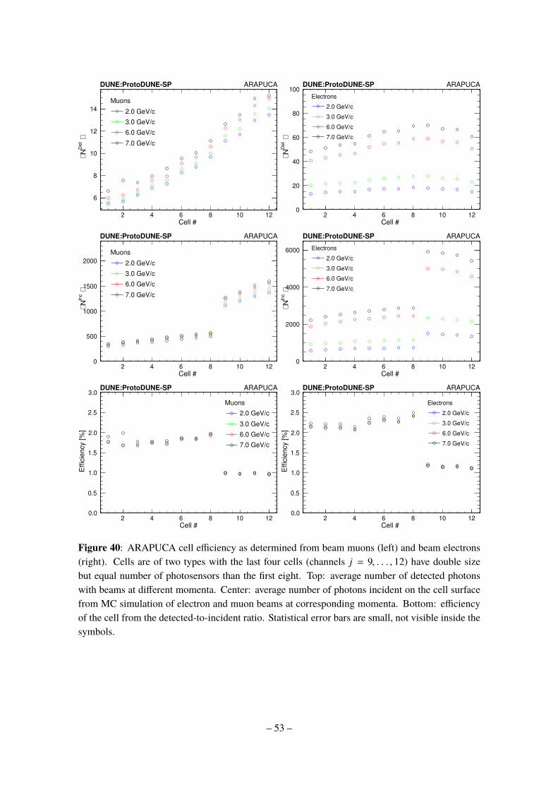
2 4 6 8 10 12Cell #

6

8

10

12

14

⟩ D

et

N⟨

Muons

2.0 GeV/c

3.0 GeV/c

6.0 GeV/c

7.0 GeV/c

DUNE:ProtoDUNE-SP ARAPUCA

2 4 6 8 10 12Cell #

0

20

40

60

80

100

⟩ D

et

N⟨

Electrons

2.0 GeV/c

3.0 GeV/c

6.0 GeV/c

7.0 GeV/c

DUNE:ProtoDUNE-SP ARAPUCA

2 4 6 8 10 12Cell #

0

500

1000

1500

2000

⟩ In

c N⟨

Muons

2.0 GeV/c

3.0 GeV/c

6.0 GeV/c

7.0 GeV/c

DUNE:ProtoDUNE-SP ARAPUCA

2 4 6 8 10 12Cell #

0

2000

4000

6000

⟩ In

c N⟨

Electrons

2.0 GeV/c

3.0 GeV/c

6.0 GeV/c

7.0 GeV/c

DUNE:ProtoDUNE-SP ARAPUCA

2 4 6 8 10 12 Cell #

0.0

0.5

1.0

1.5

2.0

2.5

3.0

Effic

iency [%

]

Muons

2.0 GeV/c

3.0 GeV/c

6.0 GeV/c

7.0 GeV/c

DUNE:ProtoDUNE-SP ARAPUCA

2 4 6 8 10 12Cell #

0.0

0.5

1.0

1.5

2.0

2.5

3.0

Effic

iency [%

]

Electrons

2.0 GeV/c

3.0 GeV/c

6.0 GeV/c

7.0 GeV/c

DUNE:ProtoDUNE-SP ARAPUCA

Figure 40: ARAPUCA cell efficiency as determined from beam muons (left) and beam electrons

(right). Cells are of two types with the last four cells (channels j = 9, . . . , 12) have double size

but equal number of photosensors than the first eight. Top: average number of detected photons

with beams at different momenta. Center: average number of photons incident on the cell surface

from MC simulation of electron and muon beams at corresponding momenta. Bottom: efficiency

of the cell from the detected-to-incident ratio. Statistical error bars are small, not visible inside the

symbols.

– 53 –

photocathode coverage partly mitigated by the light trapping in the ARAPUCA cell.

For each light-guide module in the PDS beam side the number of detected photons and incident

photons were evaluated in the same manner from the same beam muon samples (data and MC runs

with beam momenta of 2, 3, 6 and 7 GeV/c). The efficiency from the ratio of the detected to incident

photons is shown in figure 41 (left) for the 15 double-shift light-guide modules in APA3, 2 and 1

and in figure 42 (left) for the 14 dip-coated light-guide modules. Statistical error bars are small,

not visible inside the symbols. The locations of APAs 1, 2, and 3 in the ProtoDUNE-SP detector

are shown in figure 38. The efficiency of light-guide modules is expected to be proportional to the

number of suitably placed photosensors, and inversely correlated with the length of the optically

active surface of a module with fixed width due to the attenuation of internally reflected optical

photons. As a crude characterization, the smallness of the ratio of number of photosensors to

optically active surface area of the light-guide modules relative to the ARAPUCA cells underlies

the corresponding ratios of efficiencies. A factor of two can be gained by instrumenting both ends

of the light guides, but improvement beyond that would require modification to the module design

to enable effective deployment of additional photosensors.

5 10 15 Module #

0.0

0.1

0.2

0.3

0.4

0.5

0.6

Eff

icie

ncy [

%]

Muons

3GeV/c

6GeV/c

7GeV/c

DUNE:ProtoDUNE-SP Double-Shift Light Guide

5 10 15 Module #

0.0

0.1

0.2

0.3

0.4

0.5

0.6

Eff

icie

ncy [

%]

Electrons

3GeV/c

6GeV/c

7GeV/c

DUNE:ProtoDUNE-SP Double-Shift Light Guide

Figure 41: Efficiency measurements of 15 double-shift light-guide modules (PDS beam side), as

determined from beam muons (left) and beam electrons (right) data at different momenta (only

modules j = 1, .., 10 in APA3, and 2 at the shorter distance from the shower and higher photon

counting are displayed).

Electron data: electrons with beam momenta of 2, 3, 6 and 7 GeV/c provide data samples for

a second independent set of efficiency measurements. Electrons deposit all their incident energy

in showers localized in a limited portion of the LAr volume, unlike muons on long, throughgoing

tracks. Electromagnetic showers develop in front of APA3, where the ARAPUCA module is

positioned nearly at the height of the entering beam (see figure 67 with a 3D display of 7 GeV/c

beam electron event). Light detected in the ARAPUCA cells, the MC estimate of the light arriving

on the cells’ optical surfaces and the corresponding detector efficiency are shown in the right-panels

of figure 40 (top), (center) and (bottom) respectively. For any given beam energy (open circle

colors in the plots), the distribution of the detected photons by the cells along the bar exhibits

a shower-like longitudinal profile, an indication of the position reconstruction capability of the

segmented ARAPUCA module. The number of detected photons is also clearly correlated with the

– 54 –

5 10 15 Module #

0.0

0.1

0.2

0.3

0.4

Eff

icie

ncy [

%]

Muons

3GeV/c

6GeV/c

7GeV/c

DUNE:ProtoDUNE-SP Dip-Coated Light Guide

5 10 15 Module #

0.0

0.1

0.2

0.3

0.4

Eff

icie

ncy [

%]

Electrons

3GeV/c

6GeV/c

7GeV/c

DUNE:ProtoDUNE-SP Dip-Coated Light Guide

Figure 42: Efficiency measurements of 14 dip-coated light-guide modules (PDS beam side), as

determined from beam muons (left) and beam electrons (right) data at different momenta (only

modules j = 1, .., 9 in APA3, and 2 at the shorter distance from the shower and higher photon

counting are displayed).

shower energy. The calorimetric energy reconstruction from scintillation light signals is discussed

in section 7.1.

The response of the light-guide modules (beam side) to beam electrons were also used for

efficiency measurements with beam momenta of 3, 6 and 7 GeV/c, excluding electron data at

2 GeV/c with the modules in APA1 at the farthest distance from the shower and low photon

counting. Results are shown in figure 41 (right) for the ten double-shift light-guide modules in

APA3 and APA2 and in figure 42 (right) for the nine dip-coated light-guide modules.

Efficiency: the photon detection efficiency was evaluated through 8 independent measurements

using muon data and electron data at four different beam momenta, for each element of the PDS (12

cells in one ARAPUCA module, 15 double-shift light-guide modules and 14 dip-coated light-guide

modules of the PDS beam side). By comparing the results, efficiency estimated from the electron

data is found in all elements systematically higher than from the muon data, regardless of the energy

of the particle [see figures 40 (bottom), 41 and 42]. The systematic difference may be due to bias

in the MC simulation at the photon emission stage (e.g., an unaccounted deviation in scintillation

yield for GeV-scale electrons and muons with respect to minimum-ionizing particles) and at the

propagation stage (e.g., a difference due to the computational method used to approximate the

number of photons reaching the PD optical window from localized volumes (EM showers) and

long tracks (muons)). The mean value from all available measurements 〈ǫj〉 for the j-th element

is taken as the best estimate of the efficiency of that element, and the standard deviation sj that

measures the dispersion around the mean is taken as an estimate of the systematic uncertainty

on the efficiency. The statistical uncertainty, evaluated from the standard errors of the mean

numbers of detected and incident photons in the data and MC samples of muons and electrons at

different energies, is negligible. Comparing modules or cells of the same type, relative variations

in efficiency are within ±6% for the ARAPUCA cells, ±20% for the double-shift modules and

greater than ±25% for the dip-coated modules. The median efficiency value with its statistical and

systematic uncertainty from each group of detectors (ǫA, ǫA2, ǫDS, ǫDC) is selected to characterize

– 55 –

Table 4: Efficiencies of the detector technologies in the ProtoDUNE-SP PD system: median value

among detectors of the same type, determined from the average of independent measurements with

beam muons and electrons at different energies. The error is from systematic uncertainty, with

negligible statistical uncertainty. The number of detectors of different types examined correspond

to the fraction of PDS elements in the beam side upstream APAs (# 3 and 2), selected to determine

the median efficiency reported in the efficiency column.

No of PDS elements examined Detector Type Efficiency

8 ARAPUCA cell ǫA = (2.00 ± 0.25) %

4 ARAPUCA cell (double area) ǫA2 = (1.06 ± 0.09) %

10 Double-shift module ǫDS = (0.21 ± 0.03) %

9 Dip-coated module ǫDC = (0.08 ± 0.02) %

the different technologies implemented in the ProtoDUNE-SP PD system. These value are reported

in table 4. The overall relative uncertainty on the efficiency for all detector types is thus found to

be 8.5% . σǫ/ǫ . 13.5%, as determined from the set of measurements described above. This

appears compatible with the systematic error expected from uncertainty in the parameters of the

photon emission and propagation used in the MC generation.

5.3.2 Comparisons of cosmic-ray muons to simulation

The analysis of photon signals from cosmic-ray muons provides a check on the validity of the

photon simulation used to determine efficiency. Throughgoing cosmic-ray muons, or those which

enter through the upstream face and exit through the downstream face of the cryostat, are isolated

in the scintillation medium using CRT triggered events that have been matched to reconstructed

tracks in the TPC. A trigger from this sub-detector involves a four-fold coincidence of the x- and

y-measuring planes of the CRT over the span of 60 ns producing events that are very likely to contain

a throughgoing cosmic-ray muon. Two strategies were employed, both using an event definition

described by the sum of all detected photons in the twelve cells of the non-beam side ARAPUCA

module during a 13.33 µs externally tagged PDS trigger. Before either analysis, the sum of photons

per event collected at the detector surface in the simulation were scaled by a fixed amount in order

to eliminate a systematic normalization difference with data.

The first analysis, a comparison of the average light response as a function of transverse

distance, was employed to observe some of the bulk effects of the medium. Here, the transverse

distance is defined as the length of the segment between the reconstructed particle path and the

center point of the ARAPUCA module as they occupy the same position along the z axis. Since

the ARAPUCA module is in the central APA (APA6), this variable is exclusively a function of the

particle position in x and y as it bisects the detector in the z direction, exploiting the symmetry

of the detector. The results of this analysis, shown in the left plot of figure 43, suggest that the

measured data favor simulation with Rayleigh scattering length hypothesis of 90 cm as opposed

to a Rayleigh scattering length of 60 cm in the scintillation medium. A second analysis compares

each data track to a simulated track generated with matching position and trajectory in a medium

with Rayleigh scattering length set at 90 cm. Results, which are shown in the right-hand plot of

– 56 –

0.8 0.9 1.0 1.1 1.2

Data/Simulation

0

50

100

150

200

Tra

nsvers

e D

ista

nce [cm

] =60cmRL

=90cmRL

DUNE:ProtoDUNE-SP Cosmics

0

50

100

150

200

Tra

nsvers

e D

ista

nce [cm

]

0 1 2 3 4 5

Data/Simulation

0

1000

2000

3000

Events

DUNE:ProtoDUNE-SP Cosmics

Figure 43: The left-hand panel shows the ratio of the observed to the predicted PE yields as a

function of transverse distance, assuming two different values of the Rayleigh scattering length in

the simulation. The data agree more with simulation that employs a Rayleigh scattering length (LR)

of 90 cm as opposed to the 60 cm prediction. On the right, an event-by-event comparison is shown

for roughly 43,000 events taken over four months with a simulated Rayleigh scattering length of

90 cm. The dashed vertical lines in both plots represents where data and simulation agree. The

solid vertical lines in the right-hand plot represent the bounds of the plot on the left.

figure 43, demonstrate excellent agreement with simulation as a function of the transverse distance

from the ARAPUCA to the reconstructed track. In comparisons of data to simulation, one standard

deviation in the difference between the reconstructed simulated light and the measured reconstructed

light is about 18.6%. These two comparisons show that photons are successfully reconstructed in

ProtoDUNE-SP and that the simulation of the optical properties of scintillation medium is in a good

agreement with the measurements.

5.3.3 Time resolution

The timing performance of the PD system intrinsically depends upon a combination of factors, from

the intrinsic time resolution of the photosensor, to the electronics response of the readout board

and signal digitization, to the features of the light propagation, wave-length shifting and photon

collection by the PD modules. The overall timing performance is evaluated here in two different

applications: time resolution of two consecutive light signals and time matching between light

signal and TPC signal.

Resolving successive light signals in time is of importance in physics reconstruction of cor-

related events, such as stopping muon with decay to Michel electron, or kaon decays, or nucleus

de-excitation into gammas after neutrino interaction. Some of these correlations may be observed

with light signals in LAr depending on the PD timing performance. To explore this, data were taken

with an external trigger from the LCM (Light Calibration Module) producing two consecutive LED

– 57 –

flashes with a fixed time difference among them and from the common trigger time. The time dif-

ference between the pulses was set in the few µs range typical of the muon decay at rest, and much

larger than the pulse width. In figure 44 (left) a recorded waveform from the LCM trigger is shown

with the two generated consecutive LED pulses as detected by an ARAPUCA cell/12-M-MPPC

channel and digitized by the SSP readout board. The rise time of each of the two signals from the

common trigger was measured in the events collected with the LCM trigger and the distribution of

their time difference ∆t = (t2 − t1) is shown in figure 44 (right). The time resolution to observe two

separate light pulses is σ∆t ≃ 14 ns. Time jitter in the LCM pulse formation is small (sub-ns range)

and the dominant factor is from digitization (6.67 ns sampling period).

0 2 4 6 8 10 12

s]µTime [

1520

1540

1560

1580

1600

1620

1640

1660

1680

AD

C C

ount/T

ick

DUNE:ProtoDUNE-SP

Constant 7.5± 190.3

Mean 0.000± 3.333

Sigma 0.00032± 0.01376

3 3.1 3.2 3.3 3.4 3.5 3.6

s]µ t [∆

0

20

40

60

80

100

120

140

160

180

200

Events

/Tic

k

Constant 7.5± 190.3

Mean 0.000± 3.333

Sigma 0.00032± 0.01376

DUNE:ProtoDUNE-SP

Figure 44: PDS timing measurements: Double pulse light signal using the photon detector calibra-

tion system (left); Resolution in the time difference measurement between correlated light signals

(right).

3000− 2000− 1000− 0 1000 2000 3000

s)µ track time (0t

3000−

2000−

1000−

0

1000

2000

3000

s)

µP

hoto

n d

ete

cto

r tr

ack tim

e (

DUNE:ProtoDUNE-SP

flash-matched tracks

tracks not matched to flash

Figure 45: PDS Timing Measurements: Correlation between the TPC track t0 time and the PDS

flash time. Non-matched tracks (red points) are mostly from CPA-crossing vertical muons (large

negative t0) whose flash was not recorded by the PDS at the opposite end of the drift distance.

An efficient light flash-to-track matching in LArTPC is important for a correct event recon-

struction, background rejection (especially for LArTPC’s operated on the surface) and low-energy

underground physics.

– 58 –

An average of approximately 70 cosmic-ray tracks are observed overlaying each beam event

during TPC readout window. The cosmic-ray tracks arrive at random times relative to the beam

trigger. For some of these tracks, such as those that cross the cathode plane or cross one of the

anode planes, their actual time of entering the LArTPC volume (t0 time) can be reconstructed offline

from the TPC data by using the 3D track reconstruction algorithms and the geometrical features of

these CPA or APA crossing tracks. With the ProtoDUNE-SP TPC at its nominal electric field of

500 V/cm, the full drift time is 2.2 ms. Additional 2.5 ms (0.3 ms) are also recorded before (after)

the drift time period, for a total of 5 ms TPC readout window per recorded event. Cathode or anode

crossing muons have t0 time distributed over the entire recorded window and reconstructed with a

precision of about 20 µs.

PDS detected light flashes corresponding to the t0-determined TPC tracks are efficiently found

in the packets received from the SSP and contained in the PD fragment of the event. Matching

is performed in time inside the TPC readout range, looking for the closest flash timestamp to the

t0 time of the track, within a given coincidence window. In the case of CPA/APA-crossing tracks

the matching efficiency depends on the SSP discriminator threshold for the packet recording and

to the width of the coincidence window. An example of flash-to-track matching is given in figure

45, showing the bisector correlation of PDS flash time and TPC track t0 time, for a 4500 APA/CPA

crossing track sample. Tracks not matched to a flash are mostly the shorter CPA-crossing tracks

whose flash was below threshold.

6 TPC response

The high-quality ProtoDUNE-SP data will be used to measure particle-argon interaction cross

sections. Figure 46 shows various candidate events in the collection plane from ProtoDUNE-SP

data after the noise mitigation described in section 4.1 and electronics gain calibration described in

section 4.2. The color scale is in the unit of 1000 ionization electrons (ke).

It is essential to understand the charge response of wires in a LArTPC for calorimetry. In

order to measure the particle energy loss per unit length (dE/dx), it is important to correct for

nonuniformities in the detector response and determine the energy scale to convert charge to energy.

This section describes the procedure and results of the calibration of the charge and energy loss per

unit length of the ProtoDUNE-SP LArTPC. Section 6.1 discusses the calibration of space charge

effects caused by the ion accumulation in the TPC. Section 6.2 describes the measurement of drift

electron lifetime using TPC tracks and CRT information. Section 6.3 discusses the procedure to

correct for remaining nonuniformities in the detector response and determine the energy scale.

Section 6.4 shows the calibrated energy loss per unit length of different beam particles, including 1

GeV/c protons, muons, pions and electrons.

6.1 Space charge effects in ProtoDUNE-SP

As a detector located on the surface, ProtoDUNE-SP experiences a large flux of cosmic rays that

results in a substantial amount of ionization produced in the detector per unit time. Along with the

production of ionization electrons, argon ions are also produced in the detector by these cosmic

rays. Because argon ions have drift velocities on the order of several millimeters per second at

– 59 –

50 75 100 125 150 175 200Wire Number

4500

4600

4700

4800

4900

Tick

20 cm

DUNE:ProtoDUNE-SP Run 5826 Event 83959

2.5

0.0

2.5

5.0

7.5

10.0

Char

ge/ti

ck/c

hann

el (k

e)

(a) A 0.5 GeV/c electron candidate.

0 100 200 300 400Wire Number

3750400042504500475050005250

Tick

50 cm

DUNE:ProtoDUNE-SP Run 5770 Event 59001

2.5

0.0

2.5

5.0

7.5

10.0

Char

ge/ti

ck/c

hann

el (k

e)

(b) A 6 GeV/c electron candidate.

0 50 100 150 200 250 300Wire Number

3800

4000

4200

4400

4600

4800

5000

5200

Tick

30 cm

DUNE:ProtoDUNE-SP Run 5458 Event 21389

2

0

2

4

6

8

10

Char

ge/ti

ck/c

hann

el (k

e)

(c) A 1 GeV/c pion candidate.

0 100 200 300 400Wire Number

3500

3750

4000

4250

4500

4750

5000

Tick

50 cm

DUNE:ProtoDUNE-SP Run 5772 Event 15132

2

0

2

4

6

8

10

Char

ge/ti

ck/c

hann

el (k

e)

(d) A 6 GeV/c pion candidate.

60 80 100 120 140 160 180 200Wire Number

4500

4600

4700

4800

4900

5000

Tick

20 cm

DUNE:ProtoDUNE-SP Run 5387 Event 89663

2.5

0.0

2.5

5.0

7.5

10.0

Char

ge/ti

ck/c

hann

el (k

e)

(e) A 1 GeV/c stopping proton candidate.

0 100 200 300 400Wire Number

4000

4500

5000

Tick

50 cm

DUNE:ProtoDUNE-SP Run 5779 Event 12360

2.5

0.0

2.5

5.0

7.5

10.0

Char

ge/ti

ck/c

hann

el (k

e)

(f) A 2 GeV/c pion charge exchange candidate.

0 50 100 150 200 250 300Wire Number

4000

4200

4400

4600

4800

5000

5200

5400

Tick

30 cm

DUNE:ProtoDUNE-SP Run 5770 Event 29859

2

0

2

4

6

8

10

Char

ge/ti

ck/c

hann

el (k

e)

(g) A 6 GeV/c kaon candidate.

0 200 400 600 800 1000 1200 1400Wire Number

0

1000

2000

3000

4000

5000

6000

Tick

140 cm

DUNE:ProtoDUNE-SP Run 5770 Event 50648

2

0

2

4

6

8

10

Char

ge/ti

ck/c

hann

el (k

e)

(h) Large cosmic air shower candidate producingmany parallel muons.

Figure 46: Various candidate events from ProtoDUNE-SP data, with beam particles entering from

the left. The x axis shows the wire number. The y axis shows the time tick in the unit of 0.5 µs.

The color scale represents the charge deposition. The beam particle starts approximately at wire

number 90 and tick number 4800.

– 60 –

∼ 500 V/cm in liquid argon, 2–4 × 105 times slower than ionization electrons at the same electric

field, a considerable amount of positive space charge is expected in the detector as these argon

ions build up on a timescale of roughly ten minutes. A steady flux of cosmic rays ensures that

the positive ions are constantly replenished in the detector, leading to persistent distortions of the

electric field in the TPC.

These electric field distortions alter ionization electron drift paths in the detector, leading to

ionization charge being reconstructed at different positions in the detector than where the charge

originated from. The electric field distortions also impact the amount of prompt electron-ion

recombination experienced at the points of energy deposition in the detector. Both of these effects

can bias reconstructed particle energies and trajectories, and by modifying reconstructed dE/dx

along a particle track (or at the beginning of an electromagnetic shower), can lead to complications

in particle identification in a LArTPC detector. As a result, space charge effects should be carefully

characterized at any large LArTPC detector operating at or near the surface, and calibrated out when

reconstructing particle trajectories, energies and dE/dx. The observation of transverse ionization

charge migration during drift in early ProtoDUNE-SP data-taking, shown in figure 47, is consistent

with a large positive space charge density in the center of the TPC pulling ionization charge inward

toward the middle of the detector during drift toward the anode planes. This observation highlights

the fact that significant space charge effects are present at ProtoDUNE-SP and need to be addressed

when calibrating the detector. In contrast to the case of ProtoDUNE-SP, space charge effects are

expected to be negligible at the single-phase DUNE far detector due to the very low cosmic-ray rate

deep underground.

400− 300− 200− 100− 0 100 200 300 400

[cm]recoX

0

100

200

300

400

500

600

[cm

]re

co

Y

DUNE:ProtoDUNE-SP

0 100 200 300 400 500 600 700

[cm]recoZ

400−

300−

200−

100−

0

100

200

300

400

[cm

]re

co

X

DUNE:ProtoDUNE-SP

Figure 47: Projections of reconstructed and t0-tagged cosmic-ray track end points in the xy plane

(left) and zx plane (right) in ProtoDUNE-SP data; the selected tracks are t0-tagged by requiring

that they cross the cathode plane (x = 0), as described in section 4.5.2. In the absence of space

charge effects, the track end points should be reconstructed along the boundary of the TPC active

volume (dashed lines). The gaps between the APAs can also be observed in the zx plane projection

(vertical streaks in the middle of the image).

Figure 48 shows the magnitude of spatial offsets at four faces of the ProtoDUNE-SP TPC (top,

– 61 –

bottom, front or upstream with respect to the beam direction, back or downstream with respect to

the beam direction); specifically, spatial distortions in the direction normal to each detector face are

shown. These spatial distortions are estimated using the ends of reconstructed tracks that have been

t0-tagged in order to know their position in x, the ionization drift coordinate. The transverse spatial

distortion is determined by measuring the distance between the end of the track and the location of

the detector face in the direction orthogonal to the detector face being considered. As illustrated

in figure 48, spatial distortions as large as 40 cm are observed in ProtoDUNE-SP data, largest near

the faces of the TPC and furthest from the anode planes; the latter observation can be understood

as a result of charge originating further away from the anode experiencing space charge effects for

a longer time, yielding a larger impact on drift path in the detector.

0 100 200 300 400 500 600 700

recoZ

300−

200−

100−

0

100

200

300reco

X

0

5

10

15

20

25

30

35

40

Y [cm]∆Data: Top Face

DUNE:ProtoDUNE-SP

0 100 200 300 400 500 600 700

recoZ

300−

200−

100−

0

100

200

300reco

X

40−

35−

30−

25−

20−

15−

10−

5−

0

Y [cm]∆Data: Bottom Face

DUNE:ProtoDUNE-SP

300− 200− 100− 0 100 200 300

recoX

0

100

200

300

400

500

600

reco

Y

40−

35−

30−

25−

20−

15−

10−

5−

0

Z [cm]∆Data: Upstream Face

DUNE:ProtoDUNE-SP

300− 200− 100− 0 100 200 300

recoX

0

100

200

300

400

500

600

reco

Y

0

5

10

15

20

25

30

35

40

Z [cm]∆Data: Downstream Face

DUNE:ProtoDUNE-SP

Figure 48: Spatial distortions normal to the top detector face (upper left), bottom detector face

(upper right), upstream detector face (lower left), and downstream detector face (lower right) in

ProtoDUNE-SP data. The color axis represents the additive correction (in cm) one must apply to

the start/end point of a track passing through the given detector face in order to correct its position

to the true entry/exit point at the side of the detector.

A dedicated simulation of space charge effects was developed for ProtoDUNE-SP, using a

software package originally developed for MicroBooNE [56, 57]. The analysis shown in figure 48

is for data; the same analysis applied to Monte Carlo simulated events is shown in figure 49.

– 62 –

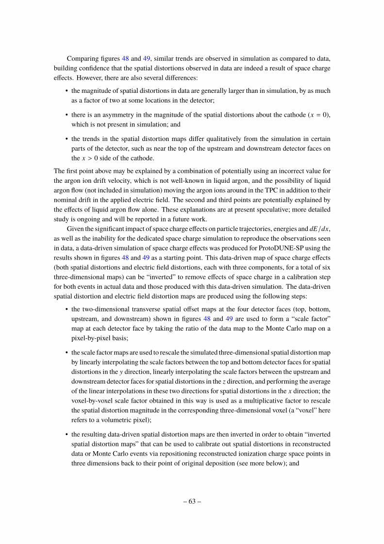
Comparing figures 48 and 49, similar trends are observed in simulation as compared to data,

building confidence that the spatial distortions observed in data are indeed a result of space charge

effects. However, there are also several differences:

• the magnitude of spatial distortions in data are generally larger than in simulation, by as much

as a factor of two at some locations in the detector;

• there is an asymmetry in the magnitude of the spatial distortions about the cathode (x = 0),

which is not present in simulation; and

• the trends in the spatial distortion maps differ qualitatively from the simulation in certain

parts of the detector, such as near the top of the upstream and downstream detector faces on

the x > 0 side of the cathode.

The first point above may be explained by a combination of potentially using an incorrect value for

the argon ion drift velocity, which is not well-known in liquid argon, and the possibility of liquid

argon flow (not included in simulation) moving the argon ions around in the TPC in addition to their

nominal drift in the applied electric field. The second and third points are potentially explained by

the effects of liquid argon flow alone. These explanations are at present speculative; more detailed

study is ongoing and will be reported in a future work.

Given the significant impact of space charge effects on particle trajectories, energies and dE/dx,

as well as the inability for the dedicated space charge simulation to reproduce the observations seen

in data, a data-driven simulation of space charge effects was produced for ProtoDUNE-SP using the

results shown in figures 48 and 49 as a starting point. This data-driven map of space charge effects

(both spatial distortions and electric field distortions, each with three components, for a total of six

three-dimensional maps) can be “inverted” to remove effects of space charge in a calibration step

for both events in actual data and those produced with this data-driven simulation. The data-driven

spatial distortion and electric field distortion maps are produced using the following steps:

• the two-dimensional transverse spatial offset maps at the four detector faces (top, bottom,

upstream, and downstream) shown in figures 48 and 49 are used to form a “scale factor”

map at each detector face by taking the ratio of the data map to the Monte Carlo map on a

pixel-by-pixel basis;

• the scale factor maps are used to rescale the simulated three-dimensional spatial distortion map

by linearly interpolating the scale factors between the top and bottom detector faces for spatial

distortions in the y direction, linearly interpolating the scale factors between the upstream and

downstream detector faces for spatial distortions in the z direction, and performing the average

of the linear interpolations in these two directions for spatial distortions in the x direction; the

voxel-by-voxel scale factor obtained in this way is used as a multiplicative factor to rescale

the spatial distortion magnitude in the corresponding three-dimensional voxel (a “voxel” here

refers to a volumetric pixel);

• the resulting data-driven spatial distortion maps are then inverted in order to obtain “inverted

spatial distortion maps” that can be used to calibrate out spatial distortions in reconstructed

data or Monte Carlo events via repositioning reconstructed ionization charge space points in

three dimensions back to their point of original deposition (see more below); and

– 63 –

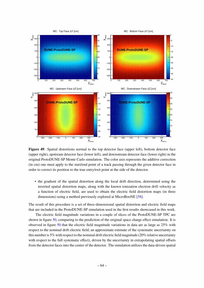
0 100 200 300 400 500 600 700

recoZ

300−

200−

100−

0

100

200

300reco

X

0

5

10

15

20

25

30

35

40

Y [cm]∆MC: Top Face

DUNE:ProtoDUNE-SP

0 100 200 300 400 500 600 700

recoZ

300−

200−

100−

0

100

200

300reco

X

40−

35−

30−

25−

20−

15−

10−

5−

0

Y [cm]∆MC: Bottom Face

DUNE:ProtoDUNE-SP

300− 200− 100− 0 100 200 300

recoX

0

100

200

300

400

500

600

reco

Y

40−

35−

30−

25−

20−

15−

10−

5−

0

Z [cm]∆MC: Upstream Face

DUNE:ProtoDUNE-SP

300− 200− 100− 0 100 200 300

recoX

0

100

200

300

400

500

600

reco

Y

0

5

10

15

20

25

30

35

40

Z [cm]∆MC: Downstream Face

DUNE:ProtoDUNE-SP

Figure 49: Spatial distortions normal to the top detector face (upper left), bottom detector face

(upper right), upstream detector face (lower left), and downstream detector face (lower right) in the

original ProtoDUNE-SP Monte Carlo simulation. The color axis represents the additive correction

(in cm) one must apply to the start/end point of a track passing through the given detector face in

order to correct its position to the true entry/exit point at the side of the detector.

• the gradient of the spatial distortion along the local drift direction, determined using the

inverted spatial distortion maps, along with the known ionization electron drift velocity as

a function of electric field, are used to obtain the electric field distortion maps (in three

dimensions) using a method previously explored at MicroBooNE [58].

The result of this procedure is a set of three-dimensional spatial distortion and electric field maps

that are included in the ProtoDUNE-SP simulation used in the first results showcased in this work.

The electric field magnitude variations in a couple of slices of the ProtoDUNE-SP TPC are

shown in figure 50, comparing to the prediction of the original space charge effect simulation. It is

observed in figure 50 that the electric field magnitude variations in data are as large as 25% with

respect to the nominal drift electric field; an approximate estimate of the systematic uncertainty on

this number is 5% with respect to the nominal drift electric field magnitude (20% relative uncertainty

with respect to the full systematic effect), driven by the uncertainty in extrapolating spatial offsets

from the detector faces into the center of the detector. The simulation utilizes the data-driven spatial

– 64 –

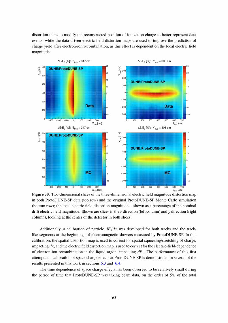
distortion maps to modify the reconstructed position of ionization charge to better represent data

events, while the data-driven electric field distortion maps are used to improve the prediction of

charge yield after electron-ion recombination, as this effect is dependent on the local electric field

magnitude.

300− 200− 100− 0 100 200 300

[cm]trueX

0

100

200

300

400

500

600

[cm

]tr

ue

Y

10−

5−

0

5

10

15

20

25

= 347 cmtrueZ [%]: 0EE/∆

DUNE:ProtoDUNE-SP

Data

0 100 200 300 400 500 600 700

[cm]trueZ

300−

200−

100−

0

100

200

300 [cm

]tr

ue

X

10−

5−

0

5

10

15

20

25

= 305 cmtrueY [%]: 0EE/∆

DUNE:ProtoDUNE-SP

Data

300− 200− 100− 0 100 200 300

[cm]trueX

0

100

200

300

400

500

600

[cm

]tr

ue

Y

10−

5−

0

5

10

15

20

25

= 347 cmtrueZ [%]: 0EE/∆

DUNE:ProtoDUNE-SP

MC

0 100 200 300 400 500 600 700

[cm]trueZ

300−

200−

100−

0

100

200

300 [cm

]tr

ue

X

10−

5−

0

5

10

15

20

25

= 305 cmtrueY [%]: 0EE/∆

DUNE:ProtoDUNE-SP

MC

Figure 50: Two-dimensional slices of the three-dimensional electric field magnitude distortion map

in both ProtoDUNE-SP data (top row) and the original ProtoDUNE-SP Monte Carlo simulation

(bottom row); the local electric field distortion magnitude is shown as a percentage of the nominal

drift electric field magnitude. Shown are slices in the z direction (left column) and y direction (right

column), looking at the center of the detector in both slices.

Additionally, a calibration of particle dE/dx was developed for both tracks and the track-

like segments at the beginnings of electromagnetic showers measured by ProtoDUNE-SP. In this

calibration, the spatial distortion map is used to correct for spatial squeezing/stretching of charge,

impacting dx, and the electric field distortion map is used to correct for the electric-field-dependence

of electron-ion recombination in the liquid argon, impacting dE . The performance of this first

attempt at a calibration of space charge effects at ProtoDUNE-SP is demonstrated in several of the

results presented in this work in sections 6.3 and 6.4.

The time dependence of space charge effects has been observed to be relatively small during

the period of time that ProtoDUNE-SP was taking beam data, on the order of 5% of the total

– 65 –

spatial distortion magnitude. A detailed study of the time dependence of space charge effects at

ProtoDUNE-SP will be presented in a future work.

6.2 Drift electron lifetime

The liquid argon of the ProtoDUNE-SP detector contains impurities, such as water and oxygen, that

can capture the ionized electrons as they drift towards the APA. Although the negative ions formed

by the attached electrons still drift to the APA, they drift much more slowly than the unattached

electrons and contribute negligibly to the signals measured on the APAs. The charge measured by

the APAs then becomes reduced due to the impurities capturing the electrons, lowering and biasing

the amount of charge measured on the wire planes. This effect is modeled as an exponential decay

as a function of time:

Q(t) = Q0 exp (−(thit − t0)/τ) , (6.1)

where Q(t) is the charge measured on a wire, Q0 is the initial charge created by the ionization of

the argon accounting for recombination, t0 is the time at which the ionization took place, thit is the

time the drifting charge arrived the APA, and τ is the drift electron lifetime. A larger value of τ

corresponds to higher liquid argon purity, as fewer drifting electrons will attach to impurities as

they drift to the APA.

Purity monitors located inside the cryostat, but outside the field cage, measure the drift electron

lifetimes for the argon inside their drift volumes, and thus are not expected to measure exactly the

drift electron lifetime in the TPC. Furtheremore, the electric field strength in the purity monitors is

lower than the electric field strength inside the TPC. Since the rate of drift electron attachment to

impurities depends on the electric field strength, the measured lifetimes in the purity monitors are

expected to further differ from that in the TPC. In situ measurements of the drift electron lifetime

from signals in the TPC therefore are needed in order to calibrate the results of charge-based

analyses.

The drift electron lifetime inside the TPC is measured by fitting the dQ/dx of collection plane

hits from cosmic-ray tracks as a function of drift times. A sample of cosmic-ray tracks that pass

through the front and back faces of the TPC and the CRT are selected. CRT data are used to

calibrate track positions and to provide timestamps for TPC tracks.

The electron lifetime measurement starts by matching a CRT track to a TPC track using the

positions of X and Y from both tracks. The timestamp from the CRT hits serve as the t0 for the TPC

track. The dQ/dx of a hit is defined to be the hit charge (Q) obtained from the area of a Gaussian

fit to the deconvolved signal divided by the step length from the previous collection plane hit to the

current collection plane hit.

To avoid the space charge effect distortions on the location of a TPC hit, the CRT track is

used to determine the hit’s position in X and Y as a function of Z, which is found through which

collection plane wire the hit occurred. The track’s position is then fed into the electric field

calibration map from figure 50. This field map corrects the dQ/dx by a scale factor based on

electric field deviations from the space charge effect. The electric field distortions from the space

charge effect were observed to cause at most a 1.75% difference in dQ/dx along the drift distance.

These calibrated measurements of dQcalibrated/dx are fitted to a Landau function convolved with a

Gaussian to find the most probable value (MPV) for 100 µs bin in time. An example of such a fit is

– 66 –

shown in figure 51. The function that describes the drift electron lifetime then can be quantified by

evaluating dQMPV/dx as such:

dQ(t)MPV

dx=

dQ0,MPV

dxexp(−(thit − tCRT)/τ) (6.2)

where adjustments in the timing are made based on the timestamp provided by the CRT.

/ ndf 2χ 70.58 / 61

Width 0.41± 11.14

MPV 0.5± 246.2

Area 5.555e+02± 3.016e+04

GSigma 0.847± 7.877

0 200 400 600 800 1000tick/cm]×dQ/dx [(ADC count)

0

100

200

300

400

500

Nu

mb

er

of

Hits

/ ndf 2χ 70.58 / 61

Width 0.41± 11.14

MPV 0.5± 246.2

Area 5.555e+02± 3.016e+04

GSigma 0.847± 7.877

/ ndf 2χ 70.58 / 61

Width 0.41± 11.14

MPV 0.5± 246.2

Area 5.555e+02± 3.016e+04

GSigma 0.847± 7.877

DUNE:ProtoDUNE-SP <1.8 mshit

1.7<t

Figure 51: Distribution of dQ/dx for a slice of 100 µs for a lower purity run in early November

2018.

Data was taken using the CRT once it became operational on November 1st, 2018 and runs

were taken with the CRT during beam data-taking from November 1st, 2018 to November 11th,

2018, the last day of beam. Fits to the MPV of the dQ/dx distributions as functions of hit time

are shown starting the first day in November and for the final day of beam data-taking in figure 52.

During the end of October 2018, the pumps that circulate and purify the liquid argon were not

operating due to an external electrical issue. The pumps resumed recirculating and purifying on

November 1st and typically take approximately a week to return the TPC back to its previous state

of liquid argon purity. Because of this circumstance, these drift electron lifetime measurements

show the structure of charge attenuation for a lower purity run and a higher purity run during purity

recovery, respectively.

While the drift electron lifetime can represent the purity, another useful metric is the ratio of

dQ/dx at the anode and cathode or Qc

Qa. This is calculated as follows:

Qc

Qa

= e−tfull drift

τ (6.3)

where tfull drift is the time it takes to drift from the cathode to the anode, which was measured to be

2.3 ms. Runs were taken with the CRT operating for the last week of beam data-taking. The Qc/Qa

was measured for each day possible and occurred during a rise in purity in the detector.

– 67 –

0.5 1.0 1.5 2.0Hit Time [ms]

150

200

250

300

350

tick/c

m]

×d

Q/d

x [

(AD

C c

ou

nt)

/ ndf 2χ 13.59 / 15

Constant 0.8618± 288

Lifetime [ms] -

e 0.2586± 10.39

/ ndf 2χ 13.59 / 15

Constant 0.8618± 288

Lifetime [ms] -

e 0.2586± 10.39

DUNE:ProtoDUNE-SP Date: 1/11/2018

0.5 1.0 1.5 2.0Hit Time [ms]

150

200

250

300

350

tick/c

m]

×d

Q/d

x [

(AD

C c

ou

nt)

/ ndf 2χ 14.39 / 15

Constant 0.6341± 281.6

Lifetime [ms] -

e 14.32± 88.95

/ ndf 2χ 14.39 / 15

Constant 0.6341± 281.6

Lifetime [ms] -

e 14.32± 88.95

DUNE:ProtoDUNE-SP Date: 11/11/2018

Figure 52: Plot the MPV of the dQ/dx distribution as a function of the hit time, fit to an exponential

decay function on November 1st, 2018 during a period of lower purity (top) and on November 11th,

2018 during a period of higher purity (bottom). Only statistical errors are included.

The systematic uncertainties determined for this measurement are from the uncertainty in the

SCE calibration and impacts diffusion have on the hits as a function of drift time. The SCE effect

uncertainty is estimated by evaluating the electron lifetime using a different SCE calibration map

measured using cosmic muons that cross the cathode and both anodes of the TPC. The difference

between the lifetime value obtained using this alternate map and the lifetime value obtained using

the SCE calibration discussed in section 6.1 is defined to be 1σ of the SCE systematic uncertainty.

– 68 –

The uncertainty due to diffusion is estimated by turning diffusion off in the Monte Carlo simulation

of the ProtoDUNE-SP detector, with a lifetime set at 35 ms. The difference in the electron lifetime

values extracted with and without diffusion in the Monte Carlo simulation is taken to be the 1σ

variation due to the diffusion systematic, and is denoted σdiff . The fractional change in the lifetime

due to diffusion is σdiff

τ= 0.143, which corresponds to a difference in Qc/Qa by 0.7%, assuming

an electron lifetime of 35 ms. This value of the fractional uncertainty in the lifetime is assumed for

all dates investigated.

Towards the beginning of data-taking Qc/Qa was measured as low as 0.801±0.026, which is

equivalent to an electron lifetime of 10.4±1.5 ms, as seen in figure 53. Toward the end of data-

taking, higher purity was achieved with a Qc/Qa of 0.9745±0.0063 on November 11th of 2018, a

value close to a 100 ms drift electron lifetime.

201801/11

201802/11

201803/11

201804/11

201805/11

201806/11

201807/11

201808/11

201809/11

201810/11

201811/11

0.4

0.6

0.8

1.0

a/Q

cQ

DUNE:ProtoDUNE-SP

3 ms

10 ms

30 ms

100 ms

Figure 53: Plot of Qc/Qa during November 2018 as measured with TPC tracks calibrated with CRT

data. Due to the run plan on November 6th, 2018, there was not enough data to make a precision

measurement of Qc/Qa on that day. Error bars include the statistical uncertainty, the uncertainty

from calibrating the SCE, and the uncertainty from diffusion’s impact on the measurement.

These electron lifetimes also approximate the amount of impurity in the detector as expressed in

units of oxygen equivalent concentration. Measurements indicate that at approximately 500 V/cm,

the impurity can be described as follows:

NO2=

1

kaτ=

300 ppt ms

τ(6.4)

with NO2being the concentration equivalent if all impurities were from oxygen and ka being the

attachment constant for oxygen [15]. Considering the inverse relationship between the drift electron

lifetime and the amount of oxygen equivalent impurity, the estimate predicts the impurity never went

above 40 ppt equivalent of oxygen in the week of data-taking. At the end of beam data-taking on

– 69 –

November 11th, 2018, the impurity in the detector can be estimated to be approximately 3.4±0.7 ppt

oxygen equivalent.

6.3 Calibration based on cosmic-ray muons

The goal of detector calibration is to convert the measured charge in units of ADC counts to

energy in units of MeV, which provides important information for particle identification and energy

measurements. In order to get reliable calorimetric information, a two-step calibration procedure is

employed following the same method developed by the MicroBooNE collaboration [59]. In the first

step, the detector response is equalized using throughgoing cosmic-ray muons. In the second step,

the absolute energy scale is determined using stopping cosmic-ray muons. In both steps muons that

cross the cathode are used because their t0 can be reconstructed (section 4.5.2). The two steps are

described in the following sections.The two steps are described in the following sections, using the

results for Run 5770 that was taken on Nov. 3, 2018 as an example.

6.3.1 Charge calibration

The charge deposition per unit length (dQ/dx) in a LArTPC is affected by a number of factors

including electronics gain variations, space charge effects, attenuation (due to electronegative

impurities like O2 and H2O), diffusion, and other effects. Some effects are calibrated out using

measurements described in previous sections such as electronics gains (section 4.2) and space

charge effects (section 6.1). Calibrating the electron lifetime in situ via cathode-crossing muons

is complicated by the very complex space charge effects. Using the CRT allowed a much more

precise calibration, but that system was not operable until late in the run and therefore those more

precise lifetime measurements were not available for runs taken before then. The effect of diffusion

has not been measured yet. In the equalization step, cathode-crossing cosmic-ray muons are used

to calibrate the residual nonuniformity in the dQ/dx values throughout the TPC after the gain and

space charge effect calibrations. The following requirements are applied for track selection:

• Fiducial volume requirements: The fiducial volume FV1 is defined as a rectangular prism

shaped as follows: the boundary from the anode planes is 10 cm, the boundary from the

upstream and downstream ends is 40 cm, and the boundary from the top and bottom of the

TPC is 40 cm. In order for a track to be selected, its start point and its end point must be

outside FV1.

• Angular requirements: The reconstruction capability of LArTPCs is limited for tracks that

are parallel to the APA wires or contained in a plane containing a wire and the electric field

direction. Figure 54 shows the dQ/dx distribution as a function of θxz and θyz , the two

angles are illustrated in figure 26. To get a sample of well reconstructed tracks, tracks with

65 < |θxz | < 115 or 70 < |θyz | < 110 are removed, as indicated by the dashed lines in

figure 54.

Tracks passing the above selection criteria are used for dQ/dx calibration. Corrections are obtained

in the yz plane and as a function of the drift distance.

– 70 –

0

50

100

150

200

250

300

350

400

tic

k/c

m]

×dQ

/dx [(A

DC

count)

200− 100− 0 100 200 [deg]

XZθ

200−

100−

0

100

200

[deg]

YZ

θx>0 Cosmics dataDUNE:ProtoDUNE-SP

(a) x > 0

0

50

100

150

200

250

300

350

400

tic

k/c

m]

×dQ

/dx [(A

DC

count)

200− 100− 0 100 200 [deg]

XZθ

200−

100−

0

100

200

[deg]

YZ

θ

x<0 Cosmics dataDUNE:ProtoDUNE-SP

(b) x < 0

Figure 54: Average dQ/dx distributions for ProtoDUNE-SP Run 5770 as functions of θxz and θyzin the collection plane. The color scale represents average dQ/dx for a track. The regions inside the

dashed lines show the track incident angles excluded for the collection plane. 106764 throughgoing

cosmic ray muon tracks were used in making the plots, which constitutes 24.8% of the total number

of cathode-crossing tracks in Run 5770.

• YZ correction factors: dQ/dx values in the yz plane are affected by many factors including

non-uniform wire response caused by nearby dead channels or disconnected wires, detector

features such as the electron diverters and the wire support combs, and transverse diffusion.

Figures 55(a) and 55(b) show the dQ/dx distribution in the yz plane separately for the x > 0

drift volume and the x < 0 drift volume. The vertical stripes in the x < 0 plot show places

where charge has been collected or distorted by the grounded electron diverters. The first

APA on the left in figure 55(b) has a lower-than average dQ/dx because of the partially-

charged disconnected G plane. The wire support combs also distort the dQ/dx averages [5],

but only by around 5%, and only in very localized positions that are narrower than the bin

sizes in the figure. To correct for these non-uniformities we divide the yz plane in the two

ProtoDUNE-SP drift volumes into a number of 5×5 cm2 bins. Considering the dQ/dx values

of all the hits lying in a particular bin, the median dQ/dx value is calculated and denoted

(dQ/dx)localYZ

. Further, the median dQ/dx value is calculated considering the hits throughout

a drift volume, which is denoted (dQ/dx)global

YZ. The YZ correction factor is then defined as

C(y, z) =(dQ/dx)global

YZ

(dQ/dx)localYZ

. (6.5)

Figures 56(a) and 56(b) show the YZ correction factors for ProtoDUNE-SP Run 5770.

• X correction factors: The dQ/dx values along the drift direction are affected by factors

such as attenuation due to electronegative impurities and longitudinal diffusion. Figure 57(a)

shows the dQ/dx distribution as a function of x. The total drift volume is divided into 5 cm

bins in the x coordinate. The dQ/dx values are first corrected using YZ correction factors

based on the y and z coordinates of the hit. After the YZ correction, the median dQ/dx

value (dQ/dx)localX

is calculated for each bin. The median dQ/dx value for the whole TPC is

– 71 –

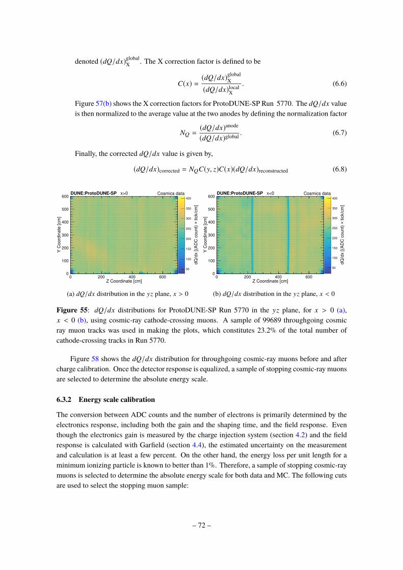
denoted (dQ/dx)global

X. The X correction factor is defined to be

C(x) =(dQ/dx)global

X

(dQ/dx)localX

. (6.6)

Figure 57(b) shows the X correction factors for ProtoDUNE-SP Run 5770. The dQ/dx value

is then normalized to the average value at the two anodes by defining the normalization factor

NQ =(dQ/dx)anode

(dQ/dx)global. (6.7)

Finally, the corrected dQ/dx value is given by,

(dQ/dx)corrected = NQC(y, z)C(x)(dQ/dx)reconstructed (6.8)

50

100

150

200

250

300

350

400 tic

k/c

m]

×dQ

/dx [(A

DC

count)

0 200 400 600Z Coordinate [cm]

0

100

200

300

400

500

600

Y C

oord

inate

[cm

]

DUNE:ProtoDUNE-SP x>0 Cosmics data

(a) dQ/dx distribution in the yz plane, x > 0

50

100

150

200

250

300

350

400

tic

k/c

m]

×dQ

/dx [(A

DC

count)

0 200 400 600Z Coordinate [cm]

0

100

200

300

400

500

600

Y C

oord

inate

[cm

]

DUNE:ProtoDUNE-SP x<0 Cosmics data

(b) dQ/dx distribution in the yz plane, x < 0

Figure 55: dQ/dx distributions for ProtoDUNE-SP Run 5770 in the yz plane, for x > 0 (a),

x < 0 (b), using cosmic-ray cathode-crossing muons. A sample of 99689 throughgoing cosmic

ray muon tracks was used in making the plots, which constitutes 23.2% of the total number of

cathode-crossing tracks in Run 5770.

Figure 58 shows the dQ/dx distribution for throughgoing cosmic-ray muons before and after

charge calibration. Once the detector response is equalized, a sample of stopping cosmic-ray muons

are selected to determine the absolute energy scale.

6.3.2 Energy scale calibration

The conversion between ADC counts and the number of electrons is primarily determined by the

electronics response, including both the gain and the shaping time, and the field response. Even

though the electronics gain is measured by the charge injection system (section 4.2) and the field

response is calculated with Garfield (section 4.4), the estimated uncertainty on the measurement

and calculation is at least a few percent. On the other hand, the energy loss per unit length for a

minimum ionizing particle is known to better than 1%. Therefore, a sample of stopping cosmic-ray

muons is selected to determine the absolute energy scale for both data and MC. The following cuts

are used to select the stopping muon sample:

– 72 –

0.8

1.0

1.2

1.4

1.6

1.8

2.0

YZ

corr

ection facto

rs

0 200 400 600Z Coordinate [cm]

0

100

200

300

400

500

600

Y C

oord

inate

[cm

]DUNE:ProtoDUNE-SP x>0 Cosmics data

(a) YZ correction factors, x > 0

0.8

1.0

1.2

1.4

1.6

1.8

2.0

YZ

corr

ection facto

rs

0 200 400 600Z Coordinate [cm]

0

100

200

300

400

500

600

Y C

oord

inate

[cm

]

DUNE:ProtoDUNE-SP x<0 Cosmics data

(b) YZ correction factors, x < 0

Figure 56: YZ correction factors for ProtoDUNE-SP Run 5770 in the yz plane, for x > 0 (a),

x < 0 (b), using cosmic-ray cathode-crossing muons.

200− 0 200X coordinate [cm]

270

280

290

300

310

tic

k/c

m]

×dQ

/dx [(A

DC

count)

DUNE:ProtoDUNE-SP Cosmics data

(a) dQ/dx vs drift dimension x

200− 0 200X coordinate [cm]

0.95

1.00

1.05

1.10

X c

orr

ection facto

rsDUNE:ProtoDUNE-SP Cosmics data

(b) X correction factors vs drift dimension x

Figure 57: dQ/dx distribution and X correction factors as a function of drift dimension x for

ProtoDUNE-SP Run 5770 (a) dQ/dx distribution and (b) X correction factors

0 200 400 600 800 1000 tick/cm]×dQ/dx [(ADC count)

0

50

100

150

)3

num

ber

of hits (

10

Calibrated dQ/dx

Uncalibrated dQ/dx

DUNE:ProtoDUNE-SP Cosmics data

Figure 58: dQ/dx distribution for throughgoing cosmic-ray muons before and after calibration

• Fiducial volume cuts: Cathode-crossing tracks which start outside FV1 and end inside a

– 73 –

smaller volume FV2 are used. The FV2 volume is a rectangular prism inside FV1 shaped as

follows: the boundary from the anode planes is 30 cm, the boundary from the upstream and

downstream ends is 50 cm, and the boundary from the top and bottom of the TPC is 50 cm.

• Angular cuts: Tracks with 65< |θxz | <115 and tracks with 70 < |θyz | <110 are

removed.

• Removing broken tracks: Some muons are reconstructed as two or more tracks, which

mimic a stopping muon. If the end points of the two tracks are within 30 cm and the angle

between them is less than 14, both tracks are removed. Additionally, any track which starts

or stops within 5 cm of an APA boundary are removed.

• Removing tracks with early and late hits: Tracks that are cut off by the 6000-tick TPC

readout window boundaries may mimic a stopping muon. If any hit associated with a track

has a peak time less than 250 ticks or greater than 5900 ticks, the track is removed.

• Removing tracks with Michel hits attached: The presence of an Michel electron can

confuse the reconstruction of the muon end point so muons that decay into Michel electrons

are removed. The Michel activities are identified by looking for isolated hits close to muon

end point. The number of hits within ±5 wires and ±50 ticks from the last hit of the muon

track and not belonging to the muon track or any other track longer than 100 cm is counted.

If the count is greater than 0, such tracks are removed.

After applying the above selection cuts, a highly pure sample of stopping muons remains.

Defining the purity as the number of true stopping muons divided by the total number of candidate

stopping muons in our sample, a purity of 99.74% is achieved based on Monte Carlo study. The

dQ/dx values are corrected as described in the previous section. The most probable dE/dx value

as a function of residual range for stopping muon tracks in LAr is accurately predicted by Landau-

Vavilov theory [60]. From the calibrated dQ/dx values (in ADC/cm) along the muon track in

its MIP region (120 to 200 cm from stopping point), the dE/dx (in MeV/cm) values are fitted

using the modified Box model [61] function to correct for the recombination effect with the charge

calibration constant Ccal (ADC×tick/cm → e/cm) as a free parameter in the χ2 minimization. Ccal is

effectively a scaling factor that accounts for the electronics gain, ADC conversion and other residual

effects that are not explicitly calibrated out. The energy loss from the stopping muon sample and a

comparison with the theoretical prediction in figure 59 show the result of the calibration procedure

for ProtoDUNE-SP Run 5770 and the corresponding Monte Carlo sample.(

dE

dx

)

calibrated

=

(

exp

(( dQdx

)calibrated

Ccal

β′Wion

ρE

)

− α) (ρE

β′

), (6.9)

where

Ccal = Calibration constant used to convert ADC values to number of electrons,

Wion = 23.6 × 10−6 MeV/electron (the work function of argon),

E = E field based on the measured space charge map,

ρ = 1.38 g/cm3 (liquid argon density at a pressure of 124.106 kPa),

α = 0.93, and

β′ = 0.212 (kV/cm)(g/cm2)/MeV.

– 74 –

α and β′ are the Modified Box model parameters which were measured by the ArgoNeuT

experiment at an electric field strength of 0.481 kV/cm [61].

The calibration constant Ccal is normalized so that the unit (“ADC×tick”) corresponds to 200

electrons. In the case where the detector response is perfectly modeled (e.g. in the simulation), the

calibration constant Ccal should be exactly 1/200 = 5×10−3 ADC×tick/e. The calibration constants

derived for the collection plane by fitting the stopping muon samples to the predicted dE/dx curve

are shown in table 5. The uncertainties are statistical only. The difference between data and MC

calibration constants is caused by the uncertainties on the gain measurement and the simulation of

detector response.

Table 5: Calibration constants for the collection plane in MC and data.

Data MC

Fitted value of Ccal (5.4 ± 0.1) ×10−3 ADC×tick/e (5.03 ± 0.01) ×10−3 ADC×tick/e

0

20

40

60

80

100

120

0 50 100 150 200Residual Range [cm]

0

1

2

3

4

5

dE

/dx [M

eV

/cm

]

DUNE:ProtoDUNE-SP Cosmics data

Expectation

(a) Data

0

10

20

30

40

50

60

70

80

90

0 50 100 150 200Residual Range [cm]

0

1

2

3

4

5

dE

/dx [M

eV

/cm

]

DUNE:ProtoDUNE-SP Cosmics MC

Expectation

(b) MC

0 2 4 6 8 10dE/dx [MeV/cm]

0.0

0.2

0.4

0.6

0.8

1.0

Rela

tive F

requency

DATA

MC

DUNE:ProtoDUNE-SP Cosmics

(c) dE/dx comparison

Figure 59: Stopping muon dE/dx distributions for the ProtoDUNE-SP cosmic-ray data and MC.

The black curves in (a) and (b) are the predicted most probable values (using the Landau-Vavilov

function) of dE/dx versus residual range and (c) is the dE/dx distribution for the stopping muon

sample. The histograms in (c) are normalized such that the maximum frequency is one.

– 75 –

6.4 Calorimetric energy reconstruction and particle identification

The calibration constants derived from cosmic-ray muons are applied to beam particles. The

following sections discuss the dE/dx distributions for beam muons and pions (section 6.4.1), beam

protons (section 6.4.2) and beam electrons (section 6.4.3). The identification of MIP particles

(muons) and non-MIP particles (protons) is discussed in section 6.4.2.

6.4.1 Identification and calorimetric energy reconstruction of 1 GeV/c beam pions and

muons

Measurements of charged pion interactions with argon nuclei are an important physics goal of

the ProtoDUNE-SP experiment. Accurate measurement of these interactions allows a more precise

understanding of neutrino interactions producing final-state pions, a key study channel of the DUNE

experiment. Reconstructing these final state pions and any particles produced by their secondary

interactions is important for estimations of neutrino energy. This section describes the results

obtained from ProtoDUNE-SP Run 5387 taken on Oct. 18, 2018 corresponding to approximately

12 hours of exposure to a 1 GeV/c beam. The electron drift lifetime of this run was approximately

14 ms as measured by the purity monitor.

Selection of events with reconstructed beam pions: The beam line instrumentation as described

in section 3 can be used to find events where the beam line has delivered a pion to the TPC. For the

1 GeV beam energy runs considered here, the beam line PID conditions for pions and muons can

be found in table 1. At a beam momentum of 1 GeV/c the measured TOF of pions and muons is

indistinguishable so the PID will select both pions and muons. Events are first removed for periods

of unstable HV or one or more inactive TPC readout boards. The Pandora pattern recognition

framework, described in section 4.5.2 is used to reconstruct the particle trajectories in the TPC as

well as identify a reconstructed particle as a likely candidate for the beam line track. To remove

events where a track has been incorrectly identified as the primary beam particle, quality cuts are

placed on the distance and angle between the end of the beam line particle’s reconstructed trajectory

and the start of the assigned reconstructed TPC beam particle track. These cuts remove backgrounds

that are not aligned with the measured beam line track such as cosmic rays and secondary particles

produced by the beam particle interacting upstream of the TPC. The cuts used for data are as follows:

• Beam quality cuts: angle

The cosine of the angle between the beam line track and reconstructed TPC track is required

to be > 0.93.

• Beam quality cuts: position

0 cm ≤ (XStartTPC

− XEndBeam

) ≤ 10 cm,

-5 cm ≤ (YStartTPC

− YEndBeam

) ≤ 10 cm,

30 cm ≤ (ZStartTPC

− ZEndBeam

) ≤ 35 cm,

where XStartTPC

is the start position in X of the reconstructed candidate beam track in the TPC

before SCE corrections. XEndBeam

is the projected X location of the intersection of the track

from the beam line instrumentation with the TPC. The cuts are not centered around zero due

the SCE shifting the start points of the reconstructed TPC tracks.

– 76 –

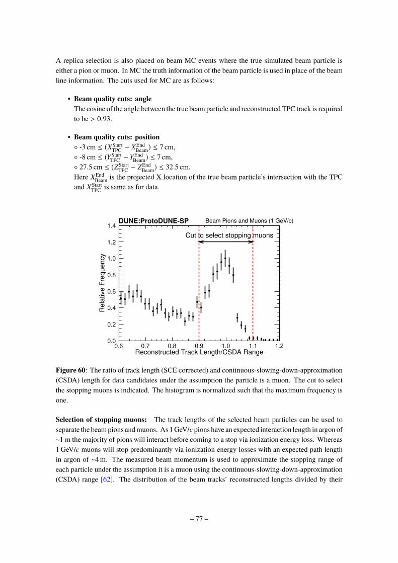
A replica selection is also placed on beam MC events where the true simulated beam particle is

either a pion or muon. In MC the truth information of the beam particle is used in place of the beam

line information. The cuts used for MC are as follows:

• Beam quality cuts: angle

The cosine of the angle between the true beam particle and reconstructed TPC track is required

to be > 0.93.

• Beam quality cuts: position

-3 cm ≤ (XStartTPC

− XEndBeam

) ≤ 7 cm,

-8 cm ≤ (YStartTPC

− YEndBeam

) ≤ 7 cm,

27.5 cm ≤ (ZStartTPC

− ZEndBeam

) ≤ 32.5 cm.

Here XEndBeam

is the projected X location of the true beam particle’s intersection with the TPC

and XStartTPC

is same as for data.

0.6 0.7 0.8 0.9 1.0 1.1 1.2Reconstructed Track Length/CSDA Range

0.0

0.2

0.4

0.6

0.8

1.0

1.2

1.4

Rela

tive F

requency

DUNE:ProtoDUNE-SP

Cut to select stopping muons

Beam Pions and Muons (1 GeV/c)

Figure 60: The ratio of track length (SCE corrected) and continuous-slowing-down-approximation

(CSDA) length for data candidates under the assumption the particle is a muon. The cut to select

the stopping muons is indicated. The histogram is normalized such that the maximum frequency is

one.

Selection of stopping muons: The track lengths of the selected beam particles can be used to

separate the beam pions and muons. As 1 GeV/c pions have an expected interaction length in argon of

~1 m the majority of pions will interact before coming to a stop via ionization energy loss. Whereas

1 GeV/c muons will stop predominantly via ionization energy losses with an expected path length

in argon of ~4 m. The measured beam momentum is used to approximate the stopping range of

each particle under the assumption it is a muon using the continuous-slowing-down-approximation

(CSDA) range [62]. The distribution of the beam tracks’ reconstructed lengths divided by their

– 77 –

calculated CSDA ranges is shown in figure 60. Requiring the ratio

0.9 <Track Length

CSDA Stopping Range< 1.1, (6.10)

selects a subsample of stopping particles, predominantly muons. A replica selection cut is placed

on the MC sample using the the simulated momentum for the true beam particle in each event as

input to the ratio calculation.

0 2 4 6 8 10dE/dX [MeV/cm]

0.0

0.2

0.4

0.6

0.8

1.0

Re

lative

Fre

qu

en

cy

DUNE:ProtoDUNE-SP

MC (SCE)

Data

Pions (1 GeV/c)

(a)

0 2 4 6 8 10dE/dX [MeV/cm]

0.0

0.2

0.4

0.6

0.8

1.0

Re

lative

Fre

qu

en

cy

DUNE:ProtoDUNE-SP

MC (SCE)

Data

Beam Stopping Muons (1 GeV/c)

(b)

Figure 61: Pion (a) and stopping muon (b) dE/dx distributions for the ProtoDUNE-SP beam

data after applying the calibration derived using cosmic-ray muons. The distribution for replica

selections on a beam Monte Carlo sample with space charge effect simulated is also shown. The

histograms are normalized such that the maximum frequency is one.

Calorimetric energy information of beam pions The charge signal calibration produced from

stopping cosmic-ray muons collected during the same run period described in section 6.3 is applied

to the selected beam tracks to calculate the true deposited energy as a function of distance (dE/dx)

along their trajectory. Figure 61(a) shows the distribution of dE/dx values of all hits on the

collection plane from the selected beam pion candidates. That is, all candidates that are not selected

by the stopping muon cut (eq. 6.10) described above. The selected particles are MIPs. The MPVs

of the calibrated data and MC samples agree to better than 1%.

Calorimetric energy information of beam stopping muons Figure 61(b) shows the distribution

of calibrated dE/dx values of all hits on the collection plane from the beam muon candidates

selected by the stopping particle cut (eq. 6.10). As with the pions, the MPVs of the data and MC

samples agree to better than 1%. The distribution of the dE/dx vs residual range for the selected

stopping muons is shown for data in figure 62(a) and for MC in figure 62(b). A clear Bragg peak is

seen at low residual range, as expected. The measured distribution displays good agreement with

the theoretical MPV curve for a stopping muon in argon, in both the minimum ionization region

and Bragg peak region of residual range.

– 78 –

0 50 100 150 200Residual Range [cm]

0

2

4

6

8

10

dE

/dX

[M

eV

/cm

]

0

50

100

150

200

250

DUNE:ProtoDUNE-SP

Expectation

Stopping Beam Muons - Data (1 GeV/c)

(a)

0

20

40

60

80

100

120

Stopping Beam Muons - MC (1 GeV/c)

0 50 100 150 200Residual Range [cm]

0

2

4

6

8

10

dE

/dX

[M

eV

/cm

]

DUNE:ProtoDUNE-SP

Expectation

Stopping Beam Muons - MC (1 GeV/c)

(b)

Figure 62: dE/dx vs residual range for selected stopping muons in the 1 GeV/c beam after applying

the calibration derived using cosmic-ray muons, in data (a) and MC (b). The expected most probable

value of dE/dx is plotted as a function of residual range for both.

6.4.2 Identification and calorimetric energy reconstruction of 1 GeV/c beam protons

To understand the detector response to protons interacting in a LArTPC, an analysis procedure,

including the selection of beam protons, detector calibration and calorimetric analysis, has been

developed. This section describes the results obtained from ProtoDUNE-SP Run 5387.

Stopping protons are used for the detector characterization in terms of calorimetry and particle

identification. Protons are selected using the same beam-TPC matching criteria described in

section 6.4.1. For the 1 GeV/c beam momentum runs considered here, the beam line PID conditions

for protons can be found in table 1.

The measured beam momentum is used to approximate the stopping range under the assumption

it is a proton using the CSDA range. Figure 63 shows the distribution of the reconstructed proton

tracks, divided by their expected CSDA ranges. The distribution peaks at 0.88, which is dominated

by the stopping protons. The peak position is less than one because of the energy loss upstream

and the SCE. The tail on the left of the distribution is due to the interacting protons, since their

drift distances inside the LAr are shorter than those of the stopping protons. The ratio cut, 0.74 ≤(reconstructed proton track length/CSDA range) ≤ 1.09, is used to select the stopping protons.

After the proton event selection, the data-driven corrections, described in section 6.1, are

applied to correct for both the spatial and the E-field distortions due to the SCE. After these

corrections, the dQ/dx values (ADC/cm) of the stopping protons are converted to the corresponding

dE/dx values (MeV/cm) using the calibration constants described in section 6.3. The same analysis

procedure is applied to a Monte Carlo sample.

Figures 64(a) and 64(b) show the energy loss versus the residual range of the stopping proton

candidates for data and MC, respectively. The data and MC after the calibration procedure show

good agreement with the expected MPVs. The distributions of dE/dx in the data and the MC are

shown in figure 64(c). The MPVs of the dE/dx distributions between data and MC agree to better

than 1%.

– 79 –

0.0 0.2 0.4 0.6 0.8 1.0 1.2 1.4Reconstructed Track Length/CSDA Range

0.0

0.2

0.4

0.6

0.8

1.0

1.2

1.4

Rela

tive F

requency

Cut to select stopping protons

DUNE:ProtoDUNE-SP Protons (1 GeV/c)

Figure 63: The distribution of the reconstructed proton track length divided by the associated

CSDA range. The histogram is normalized such that the maximum frequency is one. The incident

beam momentum is 1 GeV/c. The cut to select the stopping protons is indicated.

6.4.3 dE/dx for 1 GeV/c electrons

It is important to understand the LArTPC response to electromagnetic showers since DUNE will

measure electrons coming from oscillated neutrinos, produced via charged current interactions.

Accurate measurement of the calorimetric response of electrons in the ProtoDUNE-SP TPC allows

a more precise understanding of e/γ separation and estimation of electron neutrino energy. The

dE/dx for a photon-induced shower is expected to be twice the dE/dx of a single electron at the

beginning of the shower, due to the photon conversion into an electron-positron pair. This has been

verified in a LArTPC by the ArgoNeuT collaboration [63]. To successfully select νe charged-current

interactions in DUNE, a dE/dx metric can be used to remove electromagnetic-like background from

interactions such as neutral-current π0 production where the photons from π0 decay can mimic an

electron shower.

Electrons are selected in Run 5809 taken on Nov. 8, 2018 using the same beam-TPC matching

criteria described in section 6.4.1. For the 1 GeV/c beam momentum runs considered here, the

beam line PID conditions for electrons can be found in table 1.

The reconstruction of electron-induced showers in the detector follows the same procedure as in

track-like events. Signal processing (including deconvolution and noise removal) is followed by hit

finding and 2D cluster formation. The reconstruction framework Pandora [44] is used to reconstruct

3D showers. The position and the direction of the shower are used to define the beginning of the

shower, which is before the electromagnetic cascade develops. To ensure that the electron candidate

has not developed a cascade shower before entering the active TPC volume, a completeness cut was

required. The completeness is defined as the reconstructed shower energy divided by the incoming

electron’s momentum. Based on MC studies we expect to have losses due to energy loss upstream

and due to signal processing thresholds. If the completeness is at least 80%, the event is selected.

– 80 –

0

100

200

300

400

500

600

700

0 20 40 60 80 100 120Residual Range [cm]

0

5

10

15

20

25

30

dE

/dx [M

eV

/cm

]

Expectation

DUNE:ProtoDUNE-SP Proton Data (1 GeV/c)

(a)

0

100

200

300

400

500

0 20 40 60 80 100 120Residual Range [cm]

0

5

10

15

20

25

30

dE

/dx [

Me

V/c

m]

Expectation

DUNE:ProtoDUNE-SP Proton MC (1 GeV/c)

(b)

0 5 10 15dE/dx [MeV/cm]

0.0

0.2

0.4

0.6

0.8

1.0

1.2

Re

lative

Fre

qu

en

cy

Data

MC

DUNE:ProtoDUNE-SP Protons (1 GeV/c)

(c)

Figure 64: Stopping proton dE/dx versus residual range distributions for the ProtoDUNE-SP beam

data (a) and MC (b), the expected most probable values are shown in red. The dE/dx distributions

after the SCE corrections of data and MC are shown in (c). The histograms in (c) are normalized

such that the maximum frequency is one.

To measure dE/dx, first, the charge deposition per unit length dQ/dx is measured on a single

wire at the collection plane. To calculate the effective pitch dx between hits, the direction of

the shower is used to measure the actual distance that the electron traverses in the TPC between

adjacent wires. Then, following the discussion in section 6.1 the SCE corrections are applied.

The conversion from dQ/dx to dE/dx uses the calibration constants described in section 6.3. To

measure dE/dx at the beginning of the shower, only hits within 4 cm along the direction of the

shower and 1 cm perpendicular to the shower are considered and the median dE/dx is computed.

The same analysis procedure is applied to the Monte Carlo sample.

The dE/dx distributions for 1 GeV/c electron candidates are shown in figure 65. The dE/dx

distributions in figure 65 follow the expected Gaussian-convolved Landau distribution with the

dE/dx peak value corresponding to one single ionizing particle. This results demonstrates an

understanding of the dE/dx metric for electrons that would be a valuable input for future analyses.

Electrons are selected using the same beam-TPC matching criteria described in section 6.4.1. For

the 1 GeV/c beam momentum runs considered here, the beam line PID conditions for electrons can

– 81 –

0 2 4 6 8 10dE/dx [MeV/cm]

0.0

0.2

0.4

0.6

0.8

1.0

Rela

tive F

requency

Data

MC

DUNE:ProtoDUNE-SP Positrons (1 GeV/c)

Figure 65: dE/dx at the beginning of the shower. The histograms are normalized such that the

maximum frequency is one.

be found in table 1.

The dE/dx distributions for various particle all show a good agreement between data and MC

in the peak. However, the resolution of dE/dx is slightly overestimated in the MC. This could be

due to the imperfect modeling of physics processes and/or detector effects.

6.4.4 Particle Identification: Protons and Muons

Robust particle identification (PID) is of fundamental importance for the physics goals of ProtoDUNE-

SP and the future DUNE experiment. The calorimetric-based PID method in a LArTPC uses the

reconstructed energy deposits as a function of residual range for the stopping particles. Event selec-

tions of the stopping muons and the stopping protons are described in section 6.3.2 and section 6.4.2,

respectively. The stopping protons and muons are shown in figure 66(a). The highly-ionized protons

are clearly separated from the muons over the entire range from their stopping points.

Based on the obtained calorimetry information, a likelihood-based parameter, ζ , is adopted

to quantify the PID performance of the ProtoDUNE-SP detector. The method is to compare the

particle species with respect to the stopping proton hypothesis. The parameter ζ is defined to be:

ζ =1

nDoF

∑

j

[dEj

dx j(Data) − dEj

dx j(MC Proton)

]2

√δ2

dEj

dx j(Data) + δ2 dEj

dx j(MC Proton)

, (6.11)

where j is the j-th hit of a track and nDoF is the number of degrees of freedom.

Figure 66(b) shows the ζ distributions of the stopping protons and the stopping muons. The

protons and the muons are well-separated. The PID performance for pions is expected to be similar

to that of muons.

– 82 –

0 20 40 60 80 100 120Residual Range [cm]

5

10

15

dE

/dx [M

eV

/cm

]

0

20

40

60

80

100

120

140

160

Proton Expectation

Muon Expectation

DUNE:ProtoDUNE-SP Data

(a)

0 50 100 150 200

ζ

0.0

0.2

0.4

0.6

0.8

1.0

1.2

Rela

tive F

requency

Proton Data

Muon Data

Proton MC

Muon MC

DUNE:ProtoDUNE-SP

(b)

Figure 66: (a) dE/dx versus residual range after the SCE corrections for the stopping protons

(upper band) and the muons (lower band). The solid lines represent the expected most probable

values for the protons (red) and the muons (blue). (b) The ζ distributions of the stopping protons

and muons. The histograms are normalized such that the maximum frequency is one.

7 Photon detector response

Homogeneous calorimeters are instrumented targets where the kinetic energy (E) of incident parti-

cles is absorbed and transformed into a detectable signal. The deposited energy is typically detected

in the form of charge or light. When the energy is large enough, a shower of secondary particles

is produced (through electromagnetic or strong processes) with progressively reduced energy. If

the shower is fully contained and the output signal is efficiently collected, the calorimetric energy

resolution is expected to be good, improving with energy as 1/√

E . Calorimeters can also provide

information on shower position, direction and size as well as arrival time t0 of the particle.

A LArTPC is a sophisticated version of a homogeneous calorimeter, with additional imaging

and particle identification capabilities. Energy deposition in the liquid argon target yields free

charge from ionization and it also yields fast scintillation light. The best energy resolution would be

obtained by collecting both the charge and the light signals, which are anticorrelated by the random-

ness of the recombination processes. With detectors based on LArTPC technology, calorimetry

typically relies only on the charge signal collection, while the use of the light signal is limited to

t0 determination and triggering purposes. A first attempt to extend the use of scintillation light

for calorimetry was recently performed in a low energy range with a small sized LArTPC [64].

Operating protoDUNE-SP on the H4-VLE charged particle test beam offers the opportunity to di-

rectly probe with light the calorimetric response of liquid argon to fully contained EM and hadronic

showers in the sub- to few-GeV energy range.

7.1 Calorimetric energy reconstruction from scintillation light and energy resolution

As described in section 5.1, in ProtoDUNE-SP the photon detection system comprises a series of

optical modules positioned inside the APA frames, behind the TPC wire planes and the grounded

mesh. The active liquid argon volume is only on one side of the APA’s, on the side facing the central

– 83 –

cathode. The total photo-sensitive area is ∼ 1.5% of the boundary surface of the LAr volume.

The relatively modest optical coverage and the one-sided geometry of the PD system, compared

for example to the 4π coverage of scintillation or Cherenkov detectors, are expected to limit the

light yield and the uniformity of the calorimetric response along the drift direction. In this section,

beam electrons and data from the ARAPUCA module in the beam side of the PDS are utilized to

investigate the light yield and resolution of the ProtoDUNE-SP PD system.

Figure 67: 3D event display of a real 7 GeV beam electron in the TPC volume [only tracks inside a

predefined sub-volume (red box) are shown]. The beam electron enters near the cathode and an EM

shower develops in LAr along the beam direction, about 10 downward and 11 toward the anode

plane, where the PDS beam side modules are located inside the APA frames. Scintillation photons

from energy deposits along the shower are detected by the ARAPUCA module.

7.1.1 Beam electrons and EM showers

In a sequence of beam runs, data were collected with incident positive electrons (e+) with energies

of 0.3, 0.5, 1, 2, 3, 6 and 7 GeV, providing a large sample of EM showers developing in the LAr

volume. The beam is delivered with a typical momentum spread of ±5% around the nominal

setting. The beam line instrumentation (see section 3.3.1) provides an event-by-event particle

identification and momentum measurement with a precision of ∆p/p ≃ 2.5% [25]. Light signal

from the single beam side ARAPUCA module is used for this calorimetric response study. The

ARAPUCA module is positioned inside the upstream APA3 frame, nearly at the same height y of

the entering beam and oriented along the z axis. In figure 67 a 3D display of a 7 GeV electron

event from the ProtoDUNE-SP data sample is shown as reconstructed by the TPC. The EM shower

develops immediately downstream of the beam entry point in the LArTPC volume in front of the

ARAPUCA module, at ∼3 m distance in the x (drift) direction, and propagates longitudinally along

the beam direction, about 10 downward and 11 toward the anode plane. Scintillation light is

– 84 –

emitted isotropically from every location at which ionization occurs along the shower. The total

photo-sensitive area of the ARAPUCA module is ∼ 0.5 × 10−3 of the surface surrounding the

LArTPC active volume (beam side). Summing over the twelve cells in the ARAPUCA module,

0.3

0.5

1.0

2.0

3.0

6.0

7.0

0 1 2 3 4 5 6 7 8

[GeV]e-beamE

0 100 200 300 400 500 600 700 800 900

Ph-detectedN

81

02

17

37

81

711

511

87

99

84

51

08

69

62

05

Nu

mb

er o

f eve

nts

pe

r be

am

mo

me

ntu

m v

alu

eN

om

ina

l b

ea

m m

om

en

tum

[G

eV

/c]

ProtoDUNE - SP Electrons ARAPUCADUNE:ProtoDUNE - SP

Figure 68: Distributions of the incident beam electron energies (left) and corresponding detected

photon spectra (right) for the collected seven nominal beam energies (Gaussian fit superimposed -

red line). Fit parameters are used in figure 69. The photon spectra are relative to the sum of photons

detected by the 12 cells of the ARAPUCA PD module.

the total number of photons detected NPh =∑

NDetj

is evaluated event by event, for each beam run.

Monte Carlo events, already used for the efficiency study, are also available, generated as described

in section 5.3 with incident electrons as in the beam runs (same energy distributions and direction).

Scintillation light from the EM shower development in LAr is propagated to the photo-detector(s)

and the total number of photons incident on the surface of the ARAPUCA module is evaluated for

each event of the MC simulated momentum run. In figure 68, the energy distribution (left) of the

incident electrons from the beam spectrometer of the CERN H4-VLE beam line for each beam run

and the corresponding calorimetric response from the ARAPUCA detector (right) expressed by the

number of detected photons are shown. A Gaussian fit of both distributions (red lines in figure 68)

gives the average electron energy 〈Ee〉 and the corresponding average photon counting 〈NPh〉, and

their spreads (σE, σN ), for each run. The average number of detected photons as a function of the

beam energy is shown in figure 69. This relationship gives the calorimetric energy response from

light data. Correspondingly, the response as obtained from the MC simulation, expressed by the

– 85 –

average number of detectable photons (incident at the detector surface) from EM showers at given

electron beam energy, is presented in figure 70 (left).

To a first approximation, the average light response is a linear function of the energy over the

entire range of tested beam energies as shown in figure 69 (left) with the result of the linear fit.

The slope of the fit p1 gives the light yield Ylight = 102.1 photons/GeV. The quoted Ylight is relative

to a diffuse light source (EM shower) at a distance of about 3 m (see figure 67). The non-zero

(negative) intercept (p0 = −8.4 photons from the fit) corresponds to an incident energy offset of

−82 ± 14 MeV from the nominal value for all beam energies. From the CERN H4-VLE beam line

MC simulations (section 3.2 and 3.3) beam electrons are expected to release 10-20 MeV in the

material in the portion of the beam line downstream the spectrometer and additional ∼ 20-30 MeV

while crossing the materials inside the cryostat from the end of the beam pipe and the active volume

of the TPC (cryostat insulation and membrane, beam tube and a thin LAr layer in between). The

observed energy offset from the linear fit of the light response provides direct evidence, though in

slight excess, of the expected energy loss of beam electrons before entering the LArTPC. A slight

deviation from linearity is observed in the light response at higher incident energies, both in the

data (figure 69 - left) and in the Monte Carlo (figure 70 - left). This is due to the light response

dependence on source-to-detector distance. At higher energies, the longitudinal shower profile

extends deeper in the LAr volume along the beam direction and closer to the ARAPUCA module,

with some increase of visibility. Based on the reconstruction of the shower profile at the different

incident electron energies (see figure 40 - top-right), a geometry correction to the cells’ acceptance

has been calculated and a normalization factor applied to the data at different energies. Most of the

nonlinearity was then removed. The intercept of the linear fit after correction indicates an energy

offset of -56 ± 14 MeV, in better agreement with the expected beam electron energy loss in the

materials before entering the TPC - details of this study can be found in [65].

0 2 4 6 8 [GeV]

beam⟩

e E⟨

0

200

400

600

800

dete

cte

d⟩

Ph

N⟨

0

p 1.4±8.4 −

1p 1.5± 102.1

0

p 1.4±8.4 −

1p 1.5± 102.1

/ ndf 2χ 3.14 / 5Prob 0.68

/ ndf 2χ 3.14 / 5Prob 0.68

Electrons

Detected photons

Linear Fit

DUNE:ProtoDUNE-SP ARAPUCA

0 2 4 6 8 [GeV]

beam⟩

e E⟨

0.0

0.1

0.2

0.3

0.4

dete

cte

d⟩

Ph

N⟨/Nσ

0k 0.003± 0.062 1k 0.008± 0.099 2k 0.009± 0.057

0k 0.003± 0.062 1k 0.008± 0.099 2k 0.009± 0.057

/ ndf 2χ 5.13 / 4

Prob 0.27

/ ndf 2χ 5.13 / 4

Prob 0.27

Electrons

Detected photons

Fit function Eq.(7.1)

DUNE:ProtoDUNE-SP ARAPUCA

Figure 69: Number of detected photons (Gaussian fit mean value, from fig.68 right) as a function

of incident electron energy (Gaussian fit mean value, from fig.68 - left) (left panel). Reconstructed

energy resolution from the detected photon distributions (Gaussian fit standard deviation to the

mean ratio) (right panel). A line of slope p1 and intercept p0 is fit to the data in the left-hand plot,

and the function in equation (7.1) is fit to the data in the right-hand plot.

Based on the linearity of the light response, the relative calorimetric energy resolution σE/Ee

– 86 –

is obtained from the σN/NPh ratio of the light response (figure 69 - right). The energy resolution,

as for a homogeneous calorimeter, can be expressed in a general form [66] depending on three

different contributions:σE

E= k0 ⊕

k1√E

⊕ k2

E(7.1)

where the symbol ⊕ indicates a quadratic sum and E is in GeV. The terms on the right-hand side

are referred to below as the “constant term”, the “stochastic term” and the “noise term”. The

relative weight of the three terms depends on the energy of the incident particle. The stochastic

term contribution to the energy resolution comes from the statistical fluctuations in the number of

photons detected. The relatively large value (k1 = 9.9%) - when compared to typical homogeneous

calorimeters - is ascribed to the limited photo-sensitive coverage of the ARAPUCA module. The

noise term comes from the electronic noise of the readout chain. Its value (k2 = 0.057 GeV) is

exactly as expected from the measured signal-to-noise-ratio of the ARAPUCA readout (section

5.2.2). The constant term is large (k0 = 6.2%) and due to different contributions. The main one

comes from the incident beam electron energy spread (figure 68 - left), depending on the actual

beam line configuration (collimators aperture at different momentum setting). The mean value

of the relative energy spread σE/Ee = (5.8 ± 0.4)%. An additional contribution comes from

fluctuations in the energy loss in the materials before electrons enter the TPC. Since the energy loss

occurs downstream of the momentum spectrometer, this energy degradation and its fluctuation do

not appear in the incident beam energy spectra and it is evaluated by simulations (∼ 2%). Other

contributions to the resolution, such as non-uniformity on the detector illumination, channel to

channel response variation and possible shower leakage across the cathode, have been investigated

and shown to be negligible [65]. The light yield and resolution response obtained from a single

0 2 4 6 8 [GeV]

beam⟩

e E⟨

0

10

20

30

40

310×

incid

ent

⟩ P

h N⟨

0

q 78±693 −

1q 86± 6051

0

q 78±693 −

1q 86± 6051

/ ndf 2χ 8.37 / 5

Prob 0.14

/ ndf 2χ 8.37 / 5

Prob 0.14

Electrons

Simulation

DUNE:ProtoDUNE-SP ARAPUCA

0 2 4 6 8 [GeV]

beam⟩

e E⟨

0.6

0.8

1.0

1.2

1.4

sim

ula

ted

⟩ P

h N⟨

/

dete

cte

d⟩

Ph

N⟨

Electrons

DUNE:ProtoDUNE-SP ARAPUCA

Figure 70: Monte Carlo simulation of light response to EM showers: average number of incident

photons at the ARAPUCA bar surface from simulation vs average electron beam energy (left) and

Data/MC comparison (right) by the ratio of average number of photons detected to the corresponding

number of photons from MC simulation, at the different beam energies.

ARAPUCA module is adequate. An extrapolation of the performance to a PDS system consisting

entirely of ARAPUCA modules, obtained by scaling the detected photon response of the light

guide bars with the ratio of the ARAPUCA-to-light guide efficiencies (presented in section 5.3.1),

indicates that it can perform calorimetric energy reconstruction with an expected light yield of

– 87 –

1.9 photons/MeV. This performance exceeds the specifications of the DUNE Far Detector [5] by

almost a factor of four.

A comparison of electron data and the corresponding MC simulation can be used to validate the

simulation of the light propagation and collection. The average number of photons incident on the

surface of the ARAPUCA module from the MC (shown in figure 70 - left) is scaled by a normalization

factor η, an average value over the ARAPUCA cells’ efficiency shown in section 5.3.1, to give the

simulated detected photons 〈NPh〉simulated = η 〈NPh〉incident. The ratio 〈NPh〉detected/〈NPh〉simulated is

shown as a function of incident beam energy in figure 70 (right). A systematic deviation, between

5 and ≤ 10%, is found for electrons with energies between 0.3 GeV and 1 GeV. This deviation

is attributed to the statistical limitations on the visibility values of the photon library used in the

Monte Carlo for converting the energy deposited along the EM shower into the number of photons

impinging upon the ARAPUCA module.

8 Conclusions

This paper summarizes the first results on the performance of the ProtoDUNE-SP LArTPC using

large samples of data from a test-beam run at the CERN Neutrino Platform. The dedicated H4-VLE

beam line delivers electrons, pions, protons and kaons in the 0.3 – 7 GeV/c momentum range,

which are crucial to the study of detector performance and the measurement of particle-argon cross

sections. In table 6 the detector’s high-level performance parameters from studies and findings

presented in this report are shown and they are compared with the corresponding DUNE SP Far

Detector design specifications. For each of the categories shown, the ProtoDUNE-SP performance

meets or exceeds the DUNE specification, in several cases by a large margin. This successful

performance demonstrates the effectiveness of the single-phase detector design and the execution

of the fabrication, assembly, installation, commissioning, and operations phases [11].

Table 6: ProtoDUNE-SP performance for main parameters and corresponding DUNE specifica-

tions.

Detector parameter ProtoDUNE-SP performance DUNE specification

Average drift electric field 500 V/cm 250 V/cm (min)

500 V/cm (nominal)

LAr e-lifetime > 20 ms > 3 ms

TPC+CE

Noise (C) 550 e, (I) 650 e ENC (raw) < 1000 e ENC

Signal-to-noise 〈SNR〉 (C) 48.7, (I) 21.2 (w/CNR)

CE dead channels 0.2% < 1%

PDS light yield 1.9 photons/MeV > 0.5 photons/MeV

(@ 3.3 m distance) (@ cathode distance - 3.6 m)

PDS time resolution 14 ns < 100 ns

The electric field in the TPC drift volume was stable at the nominal level of 500 V/cm with

– 88 –

>99.5% of uptime during the data taking periods with beam and cosmics.

A drift electron lifetime in LAr in excess of 20 ms has been achieved and it was sustained for

an extended period of data-taking. It reached approximately (89 ± 22) ms for the last day of beam

data-taking. This corresponds to a concentration of impurity in the liquid argon of 3.4±0.7 ppt

oxygen equivalent. The DUNE Far Detector specification is for the impurity concentration to be

less than 100 ppt O2 equivalent.

The TPC and cold electronics show excellent signal-to-noise performance. The signal-to-noise

ratios corresponding to the most-probable-value ionization of a minimum ionizing particle are 40.3,

15.1 and 18.6, for collection, U and V wires, respectively, after noise filtering and signal processing.

The number of solidly unresponsive TPC channels was initially 29 out of 15360 and rose to

36 over the course of a year and five months of operations. Approximately 105 additional channels

are noisy or have other issues with the electronics so that they were not included in the analyses

presented in this report.

Three different photon detection technologies were implemented in the PDS and characterized

with muon and electron beam data. The ARAPUCA technology showed 2% efficiency, the highest

among the three, with a light response to EM energy deposit linear over the entire range of beam

energies. A PDS system consisting entirely of ARAPUCA modules, with an expected light yield

of 1.9 photons/MeV, will exceeds the specifications of the DUNE Far Detector.

Space-charge effects were predicted to be prominent in ProtoDUNE-SP. Spatial distortions in

the apparent positions of tracks of up to 40 cm are observed in the data, based on the points of entry

and exit into the TPC. Changes in the magnitude of the electric field by up to 25% are inferred from

the spatial distortion measurements. Data-based, three-dimensional maps of spatial offsets and

electric field strengths are made and are used to correct the observed data positions and ionization

strengths for use in precision analyses.

The measured resolutions of the calibrated TPC and photon detector responses to protons,

muons, electrons, and charged pions are similar to or better than those in the simulations that are

used to predict the performance of the first DUNE far detector module.

The data collected by ProtoDUNE-SP during beam runs and cosmic-ray runs will allow detailed

studies of detector characteristics such as fluid flow, and they will also allow the measurement of

argon-hadron cross sections. The results of these studies and measurements will be reported in

future publications.

Acknowledgments

The ProtoDUNE-SP detector was constructed and operated on the CERN Neutrino Platform. We

gratefully acknowledge the support of the CERN management, and the CERN EP, BE, TE, EN and

IT Departments for NP04/ProtoDUNE-SP. This document was prepared by the DUNE collaboration

using the resources of the Fermi National Accelerator Laboratory (Fermilab), a U.S. Department

of Energy, Office of Science, HEP User Facility. Fermilab is managed by Fermi Research Alliance,

LLC (FRA), acting under Contract No. DE-AC02-07CH11359. This work was supported by

CNPq, FAPERJ, FAPEG and FAPESP, Brazil; CFI, IPP and NSERC, Canada; CERN; MŠMT,

Czech Republic; ERDF, H2020-EU and MSCA, European Union; CNRS/IN2P3 and CEA, France;

– 89 –

INFN, Italy; FCT, Portugal; NRF, South Korea; CAM, Fundación “La Caixa” and MICINN, Spain;

SERI and SNSF, Switzerland; TÜBİTAK, Turkey; The Royal Society and UKRI/STFC, United

Kingdom; DOE and NSF, United States of America. This research used resources of the National

Energy Research Scientific Computing Center (NERSC), a U.S. Department of Energy Office of

Science User Facility operated under Contract No. DE-AC02-05CH11231.

References

[1] DUNE collaboration, S. Jones et al., Deep Underground Neutrino Experiment (DUNE), Far Detector

Technical Design Report, Volume 1 Introduction to DUNE, 2002.02967.

[2] ICARUS collaboration, S. Amerio et al., Design, construction and tests of the ICARUS T600 detector,Nucl. Instrum. Meth. A527 (2004) 329–410.

[3] DUNE collaboration, B. Abi et al., The Single-Phase ProtoDUNE Technical Design Report,1706.07081.

[4] F. Pietropaolo, Review of Liquid-Argon Detectors Development at the CERN Neutrino Platform, J.

Phys. Conf. Ser. 888 (2017) 012038.

[5] DUNE collaboration, S. Jones et al., Deep Underground Neutrino Experiment (DUNE), Far Detector

Technical Design Report, Volume IV Far Detector Single-phase Technology, 2002.03010.

[6] DUNE collaboration, B. Abi et al., Deep Underground Neutrino Experiment (DUNE), Far Detector

Technical Design Report, Volume II DUNE Physics, 2002.03005.

[7] C. Anderson et al., The ArgoNeuT Detector in the NuMI Low-Energy beam line at Fermilab, JINST 7

(2012) P10019, [1205.6747].

[8] C. Bromberg et al., Design and Operation of LongBo: a 2 m Long Drift Liquid Argon TPC, JINST 10

(2015) P07015, [1504.00398].

[9] MicroBooNE collaboration, R. Acciarri et al., Design and Construction of the MicroBooNE

Detector, JINST 12 (2017) P02017, [1612.05824].

[10] D. Adams et al., Design and performance of a 35-ton liquid argon time projection chamber as a

prototype for future very large detectors, JINST 15 (2020) P03035, [1912.08739].

[11] DUNE collaboration, Design, construction and operation of the ProtoDUNE-SP liquid argon TPC. In

preparation., 2020.

[12] D. Montanari et al., Development of membrane cryostats for large liquid argon neutrino detectors,IOP Conf. Ser. Mater. Sci. Eng. 101 (2015) 012049.

[13] P. Benetti et al., Argon purification in the liquid phase, Nucl. Instrum. Meth. A 333 (1993) 567–570.

[14] M. Adamowski et al., The Liquid Argon Purity Demonstrator, JINST 9 (2014) P07005, [1403.7236].

[15] A. Bettini, A. Braggiotti, F. Casagrande, P. Casoli, P. Cennini, S. Centro et al., A study of the factors

affecting the electron lifetime in ultra-pure liquid argon, Nuclear Instruments and Methods in Physics

Research Section A: Accelerators, Spectrometers, Detectors and Associated Equipment 305 (1991)177–186.

[16] G. J. Michna, S. P. Gent, D. Pederson, and C. Streff, “CFD Analysis of the Fluid, Heat, and ImpurityFlows in ProtoDUNE Single Phase Detector.” DUNE-Doc-17481-v1 (2019), unpublished.

– 90 –

[17] G. De Geronimo et al., Front-end ASIC for a Liquid Argon TPC, IEEE Transactions on Nuclear

Science 58 (2011) 1376–1385.

[18] D. Adams et al., The ProtoDUNE-SP LArTPC Electronics Production, Commissioning, and

Performance, JINST 15 (2020) P06017, [2002.01782].

[19] F. Acerbi and S. Gundacker, Understanding and simulating SiPMs, Nucl. Instrum. Meth. A926 (2019)16–35.

[20] E. M. Conover, Muon-induced backgrounds in the Double Chooz neutrino oscillation experiment.PhD thesis, The University of Chicago, 2014.

[21] R. Herbst et al., Design of the SLAC RCE Platform: A general purpose ATCA based data acquisition

system, in Proceedings, 21st Symposium on Room-Temperature Semiconductor X-ray and Gamma-ray

Detectors (RTSD 2014): Seattle, WA, USA, November 8-15, 2014, p. 7431254, 2016. DOI.

[22] J. Anderson et al., FELIX: a PCIe based high-throughput approach for interfacing front-end and

trigger electronics in the ATLAS Upgrade framework, JINST 11 (2016) C12023.

[23] K. Biery, C. Green, J. Kowalkowski, M. Paterno and R. Rechenmacher, artdaq: An Event-Building,

Filtering, and Processing Framework, IEEE Trans. Nucl. Sci. 60 (2013) 3764 – 3771.

[24] N. Charitonidis and I. Efthymiopoulos, Low energy tertiary beam line design for the cern neutrino

platform project, Phys. Rev. Accel. Beams 20 (Nov, 2017) 111001.

[25] A. C. Booth, N. Charitonidis, P. Chatzidaki, Y. Karyotakis, E. Nowak, I. Ortega-Ruiz et al., Particle

production, transport, and identification in the regime of 1 − 7 GeV/c, Phys. Rev. Accel. Beams 22

(Jun, 2019) 061003.

[26] I. Ortega, Accurate profile measurement of the low intensity secondary beams in the CERN

Experimental Areas. PhD thesis, Ecole Polytechnique Federale de Lausanne (EPFL), Lausanne, 2018.10.5075/epfl-thesis-8278.

[27] “FMC Time to Digital Converter | FMC TDC 1ns 5cha.”https://ohwr.org/project/fmc-tdc/wikis/home.

[28] N. Charitonidis, I. Efthymiopoulos and Y. Karyotakis, Beam performance and instrumentation

studies for the ProtoDUNE-DP experiment of CENF, Tech. Rep. CERN-ACC-NOTE-2016-0052. 27,CERN, Geneva, Jul, 2016.

[29] N. Charitonidis, Y. Karyotakis and L. Gatignon, Estimation of the R134a gas refractive index for use

as a Cherenkov radiator, using a high energy charged particle beam, Nuclear Instruments and

Methods in Physics Research Section B: Beam Interactions with Materials and Atoms 410 (2017) 134– 138.

[30] D. Carey, K. Brown and F. Rothacker, "third-order transport: A computer program for designing

charged particle beam transport systems", technical report, Stanford Linear Accelerator Center,Menlo Park, CA (US), 1995. 10.2172/97260.

[31] “Methodical Accelerator Design CERN.” http://mad.web.cern.ch/mad/.

[32] P. K. Skowronski, F. Schmidt and E. Forest, Advances in MAD X using PTC, Conf. Proc. C070625

(2007) 3381.

[33] P. Chatzidaki, Optics optimization of tertiary particle beamlines and efficiency measurement of

prototype scintillating fiber detectors. Diploma thesis, Natl. Tech. U., Athens, Oct, 2018.

[34] T. J. Roberts, K. B. Beard, D. Huang, S. Ahmed, D. M. Kaplan and L. K. Spentzouris, G4Beamline

Particle Tracking in Matter-dominated Beam Lines, Conf. Proc. C0806233 (2008) WEPP120.

– 91 –

[35] T. Böhlen, F. Cerutti, M. Chin, A. Fassò, A. Ferrari, P. Ortega et al., The FLUKA Code:

Developments and Challenges for High Energy and Medical Applications, Nuclear Data Sheets 120

(2014) 211 – 214.

[36] A. Ferrari, P. R. Sala, A. Fassò and J. Ranft, FLUKA: A multi-particle transport code (program

version 2005). CERN Yellow Reports: Monographs. CERN, Geneva, 2005,10.5170/CERN-2005-010.

[37] MicroBooNE collaboration, R. Acciarri et al., Noise Characterization and Filtering in the

MicroBooNE Liquid Argon TPC, JINST 12 (2017) P08003, [1705.07341].

[38] S. Ramo, Currents induced by electron motion, Proc. Ire. 27 (1939) 584–585.

[39] R. Veenhof, GARFIELD, recent developments, Nucl. Instrum. Meth. A 419 (1998) 726.

[40] Y. Li et al., Measurement of Longitudinal Electron Diffusion in Liquid Argon, Nucl. Instrum. Meth.

A816 (2016) 160–170, [1508.07059].

[41] C. Zhang, “Summary of Liquid Argon Properties.” http://lar.bnl.gov/properties/.

[42] MicroBooNE collaboration, C. Adams et al., Ionization electron signal processing in single phase

LArTPCs. Part I. Algorithm Description and quantitative evaluation with MicroBooNE simulation,JINST 13 (2018) P07006, [1802.08709].

[43] MicroBooNE collaboration, C. Adams et al., Ionization electron signal processing in single phase

LArTPCs. Part II. Data/simulation comparison and performance in MicroBooNE, JINST 13 (2018)P07007, [1804.02583].

[44] J. S. Marshall and M. A. Thomson, The Pandora Software Development Kit for Pattern Recognition,Eur. Phys. J. C75 (2015) 439, [1506.05348].

[45] MicroBooNE collaboration, R. Acciarri et al., The Pandora multi-algorithm approach to automated

pattern recognition of cosmic-ray muon and neutrino events in the MicroBooNE detector, Eur. Phys.

J. C78 (2018) 82, [1708.03135].

[46] A. A. Machado and E. Segreto, ARAPUCA a new device for liquid argon scintillation light detection,JINST 11 (2016) C02004.

[47] Z. Moss, J. Moon, L. Bugel, J. M. Conrad, K. Sachdev, M. Toups et al., A Factor of Four Increase in

Attenuation Length of Dipped Lightguides for Liquid Argon TPCs Through Improved Coating,1604.03103.

[48] L. Bugel, J. M. Conrad, C. Ignarra, B. J. P. Jones, T. Katori, T. Smidt et al., Demonstration of a

Lightguide Detector for Liquid Argon TPCs, Nucl. Instrum. Meth. A640 (2011) 69–75, [1101.3013].

[49] B. Howard, S. Mufson, D. Whittington, B. Adams, B. Baugh, J. R. Jordan et al., A Novel Use of Light

Guides and Wavelength Shifting Plates for the Detection of Scintillation Photons in Large Liquid

Argon Detectors, Nucl. Instrum. Meth. A907 (2018) 9–21, [1710.11233].

[50] L. Condat, A Direct Algorithm for 1D Total Variation Denoising, IEEE Signal Processing Letters 20

(2013) 1054–1057.

[51] E. D. Church, LArSoft: A Software Package for Liquid Argon Time Projection Drift Chambers,1311.6774.

[52] C. Zhang, “Wire-Cell BEE event display.” https://www.phy.bnl.gov/twister/bee.

[53] T. Doke, A. Hitachi, J. Kikuchi, K. Masuda, H. Okada and E. Shibamura, Absolute Scintillation Yields

in Liquid Argon and Xenon for Various Particles, Jap. J. Appl. Phys. 41 (2002) 1538–1545.

– 92 –

[54] M. Babicz et al., Experimental study of the propagation of scintillation light in Liquid Argon, Nucl.

Instrum. Meth. A936 (2019) 178–179.

[55] M. Babicz et al., Light Propagation in Liquid Argon, 2002.09346.

[56] M. Mooney, The MicroBooNE Experiment and the Impact of Space Charge Effects, in Proceedings,

Meeting of the APS Division of Particles and Fields (DPF 2015): Ann Arbor, Michigan, USA, 4-8

Aug 2015, 2015. 1511.01563.

[57] MicroBooNE Collaboration, “Measurement of Space Charge Effects in MicroBooNE.”http://microboone.fnal.gov/public-notes/ (see MICROBOONE-NOTE-1018-PUB).

[58] MicroBooNE collaboration, C. Adams et al., A Method to Determine the Electric Field of Liquid

Argon Time Projection Chambers Using a UV Laser System and its Application in MicroBooNE,1910.01430.

[59] MicroBooNE collaboration, C. Adams et al., Calibration of the charge and energy loss per unit

length of the MicroBooNE liquid argon time projection chamber using muons and protons, JINST 15

(2020) P03022, [1907.11736].

[60] Particle Data Group collaboration, M. Tanabashi, K. Hagiwara, K. Hikasa, K. Nakamura,Y. Sumino, F. Takahashi et al., Review of particle physics, Phys. Rev. D 98 (Aug, 2018) 030001.

[61] ArgoNeuT collaboration, R. Acciarri et al., A Study of Electron Recombination Using Highly

Ionizing Particles in the ArgoNeuT Liquid Argon TPC, JINST 8 (2013) P08005, [1306.1712].

[62] “Muon Stopping Power and Range Tables 10 MeV - 100TeV.”http://pdg.lbl.gov/2019/AtomicNuclearProperties/adndt.pdf.

[63] ArgoNeuT Collaboration collaboration, R. Acciarri, C. Adams, J. Asaadi, B. Baller, T. Bolton,C. Bromberg et al., First observation of low energy electron neutrinos in a liquid argon time

projection chamber, Phys. Rev. D 95 (Apr, 2017) 072005.

[64] LArIAT collaboration, W. Foreman et al., Calorimetry for low-energy electrons using charge and

light in liquid argon, Phys. Rev. D101 (2020) 012010, [1909.07920].

[65] D. Totani and F. Cavanna, First Calorimetric Energy Reconstruction of Beam Events with ARAPUCA

Light Detector in ProtoDUNE-SP, JINST 15 (2020) C03033.

[66] C. W. Fabjan and F. Gianotti, Calorimetry for particle physics, Rev. Mod. Phys. 75 (2003) 1243–1286.

– 93 –