Are the twin or triple deficits hypotheses applicable to post ...
44
Şen, Hüseyin; Kaya, Ayşe Working Paper Are the twin or triple deficits hypotheses applicable to post-communist countries? BOFIT Discussion Papers, No. 3/2016 Provided in Cooperation with: Bank of Finland, Helsinki Suggested Citation: Şen, Hüseyin; Kaya, Ayşe (2016) : Are the twin or triple deficits hypotheses applicable to post-communist countries?, BOFIT Discussion Papers, No. 3/2016, ISBN 978-952-323-091-0, Bank of Finland, Institute for Economies in Transition (BOFIT), Helsinki, https://nbn-resolving.de/urn:NBN:fi:bof-201602251031 This Version is available at: http://hdl.handle.net/10419/212846 Standard-Nutzungsbedingungen: Die Dokumente auf EconStor dürfen zu eigenen wissenschaftlichen Zwecken und zum Privatgebrauch gespeichert und kopiert werden. Sie dürfen die Dokumente nicht für öffentliche oder kommerzielle Zwecke vervielfältigen, öffentlich ausstellen, öffentlich zugänglich machen, vertreiben oder anderweitig nutzen. Sofern die Verfasser die Dokumente unter Open-Content-Lizenzen (insbesondere CC-Lizenzen) zur Verfügung gestellt haben sollten, gelten abweichend von diesen Nutzungsbedingungen die in der dort genannten Lizenz gewährten Nutzungsrechte. Terms of use: Documents in EconStor may be saved and copied for your personal and scholarly purposes. You are not to copy documents for public or commercial purposes, to exhibit the documents publicly, to make them publicly available on the internet, or to distribute or otherwise use the documents in public. If the documents have been made available under an Open Content Licence (especially Creative Commons Licences), you may exercise further usage rights as specified in the indicated licence.
-
Upload
khangminh22 -
Category
Documents
-
view
4 -
download
0
Transcript of Are the twin or triple deficits hypotheses applicable to post ...

Şen, Hüseyin; Kaya, Ayşe
Working Paper
Are the twin or triple deficits hypotheses applicable topost-communist countries?
BOFIT Discussion Papers, No. 3/2016
Provided in Cooperation with:Bank of Finland, Helsinki
Suggested Citation: Şen, Hüseyin; Kaya, Ayşe (2016) : Are the twin or triple deficits hypothesesapplicable to post-communist countries?, BOFIT Discussion Papers, No. 3/2016, ISBN978-952-323-091-0, Bank of Finland, Institute for Economies in Transition (BOFIT), Helsinki,https://nbn-resolving.de/urn:NBN:fi:bof-201602251031
This Version is available at:http://hdl.handle.net/10419/212846
Standard-Nutzungsbedingungen:
Die Dokumente auf EconStor dürfen zu eigenen wissenschaftlichenZwecken und zum Privatgebrauch gespeichert und kopiert werden.
Sie dürfen die Dokumente nicht für öffentliche oder kommerzielleZwecke vervielfältigen, öffentlich ausstellen, öffentlich zugänglichmachen, vertreiben oder anderweitig nutzen.
Sofern die Verfasser die Dokumente unter Open-Content-Lizenzen(insbesondere CC-Lizenzen) zur Verfügung gestellt haben sollten,gelten abweichend von diesen Nutzungsbedingungen die in der dortgenannten Lizenz gewährten Nutzungsrechte.
Terms of use:
Documents in EconStor may be saved and copied for yourpersonal and scholarly purposes.
You are not to copy documents for public or commercialpurposes, to exhibit the documents publicly, to make thempublicly available on the internet, or to distribute or otherwiseuse the documents in public.
If the documents have been made available under an OpenContent Licence (especially Creative Commons Licences), youmay exercise further usage rights as specified in the indicatedlicence.

BOFIT Discussion Papers 3 • 2016
Hüseyin Şen and Ayşe Kaya
Are the twin or triple deficits hypotheses applicable to post-communist countries?
Bank of Finland, BOFIT Institute for Economies in Transition

BOFIT Discussion Papers Editor-in-Chief Zuzana Fungáčová BOFIT Discussion Papers 3/2016 18.2.2016 Hüseyin Şen and Ayşe Kaya: Are the twin or triple deficits hypotheses applicable to post-communist countries? ISBN 978-952-323-091-0, online ISSN 1456-5889, online This paper can be downloaded without charge from http://www.bof.fi/bofit. Suomen Pankki Helsinki 2016
BOFIT- Institute for Economies in Transition Bank of Finland
BOFIT Discussion Papers 3/ 2016
3
Contents
Abstract ................................................................................................................................. 4
1 Introduction .................................................................................................................... 5
2 Macroeconomic backgrounds of six post-communist countries .................................... 6
3 Theoretical and empirical backgrounds to the study .................................................... 10
3.1 Theoretical background ......................................................................................... 10
3.2 Empirical background ........................................................................................... 13
4 Data set, variables, and methodology ........................................................................... 15
4.1 Data set and variables ............................................................................................ 15
4.2 Methodology: bootstrap panel Granger causality test ........................................... 16
5 Empirical results and discussion .................................................................................. 18
6 Concluding remarks ..................................................................................................... 23
References ........................................................................................................................... 26
Appendices .......................................................................................................................... 30
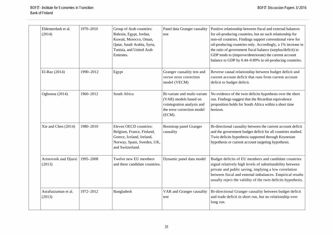
Appendix A Selected empirical studies on twin and triple deficits hypotheses .......... 30
Appendix B Cross-sectional dependence and slope homogeneity tests ...................... 38
Appendix C Other results from bootstrap panel Granger causality analysis ............... 41

Hüseyin Şen and Ayşe Kaya Are the twin or triple deficits hypotheses applicable to post-communist countries?
4
Hüseyin Şen and Ayşe Kaya
Are the twin or triple deficits hypotheses applicable to post-communist countries?
Abstract This study empirically examines the validity of the twin and triple deficits hypotheses using bootstrap panel Granger causality analysis and an annual panel data set of six post-com-munist countries (Russia, Poland, Ukraine, Romania, the Czech Republic, and Hungary) from 1994 to 2012. Our findings, based on panel data analysis under cross-sectional dependence and country-specific heterogeneity, support neither the twin deficits hypothesis nor its ex-tended version, the triple deficits hypothesis, for any of the countries considered. In other words, we find no Granger-causal relationship between budget deficits and trade (or current account) deficits or among budget deficits, private savings-investment deficits, and trade deficits.
JEL codes: E60, F30, F32, H62. Keywords: macroeconomic policy, fiscal policy, twin deficits, triple deficits, post-com-munist countries, transition economies, bootstrap panel granger causality test.
Hüseyin Şen, orcid.org/0000-0002-9833-824X, (corresponding author). Yıldırım Beyazıt University, Faculty of Political Sciences, Public Finance Department, Cinnah Caddesi, No:16, 06690 Çankaya, Ankara/Turkey. E-mail: [email protected], Phone: +90 312 466 75 33, ext. 3567.
Ayşe Kaya, orcid.org/0000-0002-7025-1775. İzmir Kâtip Çelebi University, Faculty of Economics and Ad-ministrative Sciences, Public Finance Department, Çiğli Ana Yerleşkesi, 35600, İzmir/Turkey. E-mail: [email protected].
Hüseyin Şen conducted much of this study as a visiting researcher at the Bank of Finland. The views expressed here are those of the authors and do not necessarily reflect the views of the Bank of Finland. We thank the Bank of Finland, and Laura Solanko, Zuzana Fungacova and Tia Kurtti of BOFIT in particular, for their generous assistance. We are also extremely grateful to László Kónya from the University of La Trobe, School of Economics, for making available his TSP codes.

BOFIT- Institute for Economies in Transition Bank of Finland
BOFIT Discussion Papers 3/ 2016
5
1 Introduction The twin deficit hypothesis proposes that budget deficits and trade (or current account) def-icits of an economy are intertwined. Deterioration in the budget balance results eventually in a corresponding deterioration of the trade (or current account) balance of an economy. Whether in the context of the recent Eurozone crisis or US Congressional wrangling over the debt ceiling, this unresolved postulate is invoked repeatedly in framing macroeconomic policy discussions.
The twin deficits hypothesis gained popularity in the US in the early 1980s at a time when large chronic current account deficits were accompanied by widening US budget def-icits. In 1984, Martin Feldstein, during his chairmanship of President Ronald Reagan’s Council of Economic Advisers (Frankel, 2006) termed the co-existence and tandem move-ment of budget deficits and trade (or current account deficits) “twin deficits.” According to Feldstein (1992), side-by-side depictions of budget and trade deficits produced an image of inseparable “Siamese twins.”
In the US case, the twin deficits hypothesis re-emerges in wide political discussion whenever the US is experiencing worsening trade deficits. Some of this may be ascribed to its populist appeal. As Gregory Mankiw noted in a December 2005 speech during his stint as head of George W. Bush’s economics team: “From the perspective of the Beltway mer-cantilists, the trade deficit is a huge national problem. They look at the trade deficit simply as lost jobs for Americans.” (Mankiw, 2006: 680). Trade deficits can be problematic for most nations, of course, so it is hardly surprising that the twin-deficits linkage has found its way into macroeconomic policy conversations around the world.
In recent years, a “triple deficits” hypothesis that includes the private savings-in-vestment gap has emerged. Simply put, the triple deficits hypothesis proposes a linkage among government budget balance, savings-investment balance, and foreign trade (or cur-rent account) balance of an economy. Accordingly, government budget deficit along with savings-investment deficit (i.e. the economy-wide resource gap) induces trade (or current account) deficits. “Triple deficits” refers to the case where the domestic imbalance (simul-taneous budget and private savings-investment deficits) is accompanied by an external im-balance (trade or current account deficits). To the best of our knowledge, Szakolczai (2006) may be credited for introducing the term “triple deficits” into wide use.
The relationship of budget deficits, private savings-investment deficits, and trade (or current account) deficits is a natural topic of interest for academics and policymakers. Understanding possible causal relationships among these variables is a pre-condition for de-signing robust macroeconomic policies and creating policies that promote macroeconomic stability and economic growth. It is also generally accepted that large and persistent deficits threaten macroeconomic stability and growth. Indeed, as the experiences of many countries
Hüseyin Şen and Ayşe Kaya Are the twin or triple deficits hypotheses applicable to post-communist countries?
6
have shown, large and persistent budget deficits cause serious problems for future genera-tions by leaving them with a repayment burden. Similarly, large and persistent budget and trade deficits are problematic for countries when they drain their currency reserves, cause them to take on excessive debt, or set the stage for an economic crisis.
Perhaps the largest perceived threat of dual budget and trade (or current account) deficits, however, is their ability to induce macroeconomic imbalances that damage the long-run economic development trend of a country. This concern was prominent among policy-makers in European transition economies two decades ago, when their countries faced huge initial distortions and there was great potential to run sizable trade and budget deficits for many years.
In the following analysis, we consider the validity of the twin deficits hypothesis and its cousin the triple deficits hypothesis in the context of six European transition econo-mies (Russia, Poland, Ukraine, Romania, the Czech Republic, and Hungary). To the best of our knowledge, this is the first analysis attempting to examine the double and triple deficits hypotheses for these transition economies. We also employ bootstrap panel Granger causal-ity analysis, a recent technique proposed by Kónya (2006) that allows for simultaneous anal-ysis of Granger causality between two or three variables. The bootstrap panel Granger cau-sality approach is based on a seemingly unrelated regression (SUR) estimation that considers cross-sectional dependence across countries. In practice, it means we can test Granger cau-sality for each country by taking into account the possible contemporaneous correlation across countries. The approach is also based on a Wald test with country-specific bootstrap critical values, so it does not require a joint hypothesis for all members of the panel.
The rest of the study is divided into four parts. Section 2 briefly outlines the mac-roeconomic developments of the countries in our sample. Section 3 introduces the theoretical motivation and previous empirical findings on the twin and triple deficits hypotheses. Sec-tion 4 describes the data set, variables and methodology of the study, while Section 5 reports empirical results and discussion. Section 6 presents concluding remarks.
2 Macroeconomic backgrounds of six post-communist countries In the aftermath of the collapse of the Soviet Union, a number of formerly socialist countries embarked on the long and painful transition process to market-based economies similar to their Western counterparts. The speed of the transition process has varied considerably across our six sample transition countries. In Poland and Russia, the process was quite rapid, and nearly as fast in Czechoslovakia. Hungary, a relatively more liberalized country, had less need for rapid change, so progress was slower. Romania and Ukraine faced resistance to reforms from pressure and interest groups. Nevertheless, all of these countries eventually

BOFIT- Institute for Economies in Transition Bank of Finland
BOFIT Discussion Papers 3/ 2016
7
implemented reforms, ranging from macroeconomic stabilization to designing new market institutions and establishing new legal infrastructures. The core of reforms to increase effi-ciency and stimulate growth comprised macroeconomic stabilization, price and foreign trade liberalization, restructuring and privatizing state owned enterprises, and fundamental redefinition of the state’s role (IMF, 2000).
During the first decade of transition, most countries struggled with high inflation and recession, which were to some extent side effects of price liberalization and the sudden collapse of economic linkages. Output fell dramatically in nearly all Eastern European tran-sition countries. At the same time, the lifting price controls and liberalization of trade left industrial firms, in particular, facing serious liquidity problems and falling demand. In addi-tion to poor economic performance, transition countries neglected critical reform areas such as governance, restructuring and privatizing state-owned enterprises, setting up open labor markets, and developing viable competition policies. Some of the political timidity in mov-ing ahead with institution-building reflected opposition pressure and interest groups that rightfully or not feared change.
In any case, virtually all Eastern European countries performed poorly in their first decade of transition. Policies tended to focus on the low-hanging fruit of industrial growth revival, rather than the harder-to-reach challenge of correcting macroeconomic imbalances. Thus, monetary and fiscal policies in these countries created large demand for inadequate goods and services. With persistent excess demand, these countries encountered serious mac-roeconomic problems, including output gaps, unsustainable external debt, and high inflation.
Given the lack of monetary policy tools, transition countries initially adopted pegged exchange rate regimes. As time went on, they migrated to intermediate exchange rate regimes and eventually managed floats that recognized the potential destabilizing effects of international capital inflows and minimized negative effects on exports. In the initial one or two years of transition, all of our sample countries adopted conventional fixed pegs. In subsequent years, they migrated to export-oriented exchange rate regimes, such as crawling pegs, crawling bands or managed floats without pre-announced exchange rate trajectories. Although none of these arrangements provides a stable exchange rate regime, our four sam-ple countries that joined the EU (Hungary, Poland, Romania, and the Czech Republic) all eventually adopted independent floating regimes. Russia, in contrast, employed a managed float throughout most of the observation period. Ukraine has tried several exchange rate regimes, including fixed peg and independent float.
Russia’s 1998 financial crisis negatively affected all our sample countries, most notably in the form of a collapse in Russian imports. Ukraine was hit hardest, due to its close trade ties with Russia. All sample countries devalued their currencies or abandoned their existing exchange rate regime following large ruble devaluations and all experienced subse-quent declines in growth.
Hüseyin Şen and Ayşe Kaya Are the twin or triple deficits hypotheses applicable to post-communist countries?
8
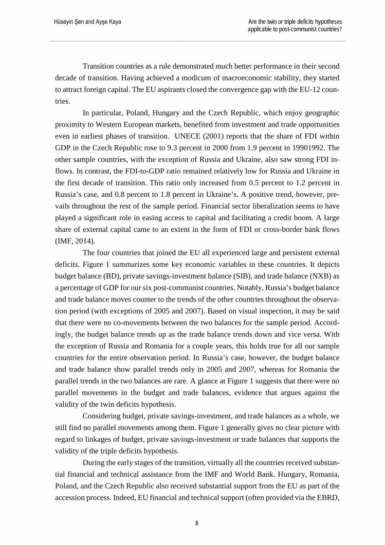
Transition countries as a rule demonstrated much better performance in their second decade of transition. Having achieved a modicum of macroeconomic stability, they started to attract foreign capital. The EU aspirants closed the convergence gap with the EU-12 coun-tries.
In particular, Poland, Hungary and the Czech Republic, which enjoy geographic proximity to Western European markets, benefited from investment and trade opportunities even in earliest phases of transition. UNECE (2001) reports that the share of FDI within GDP in the Czech Republic rose to 9.3 percent in 2000 from 1.9 percent in 19901992. The other sample countries, with the exception of Russia and Ukraine, also saw strong FDI in-flows. In contrast, the FDI-to-GDP ratio remained relatively low for Russia and Ukraine in the first decade of transition. This ratio only increased from 0.5 percent to 1.2 percent in Russia’s case, and 0.8 percent to 1.8 percent in Ukraine’s. A positive trend, however, pre-vails throughout the rest of the sample period. Financial sector liberalization seems to have played a significant role in easing access to capital and facilitating a credit boom. A large share of external capital came to an extent in the form of FDI or cross-border bank flows (IMF, 2014).
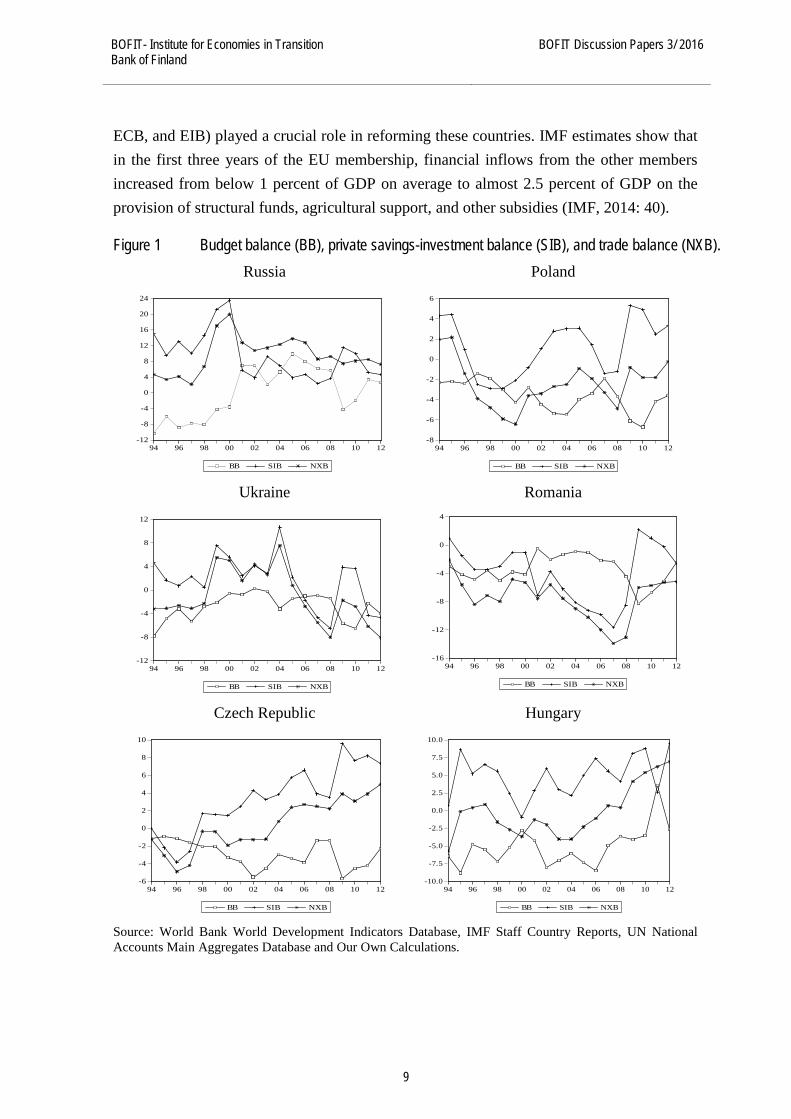
The four countries that joined the EU all experienced large and persistent external deficits. Figure 1 summarizes some key economic variables in these countries. It depicts budget balance (BD), private savings-investment balance (SIB), and trade balance (NXB) as a percentage of GDP for our six post-communist countries. Notably, Russia’s budget balance and trade balance moves counter to the trends of the other countries throughout the observa-tion period (with exceptions of 2005 and 2007). Based on visual inspection, it may be said that there were no co-movements between the two balances for the sample period. Accord-ingly, the budget balance trends up as the trade balance trends down and vice versa. With the exception of Russia and Romania for a couple years, this holds true for all our sample countries for the entire observation period. In Russia’s case, however, the budget balance and trade balance show parallel trends only in 2005 and 2007, whereas for Romania the parallel trends in the two balances are rare. A glance at Figure 1 suggests that there were no parallel movements in the budget and trade balances, evidence that argues against the validity of the twin deficits hypothesis.
Considering budget, private savings-investment, and trade balances as a whole, we still find no parallel movements among them. Figure 1 generally gives no clear picture with regard to linkages of budget, private savings-investment or trade balances that supports the validity of the triple deficits hypothesis.
During the early stages of the transition, virtually all the countries received substan-tial financial and technical assistance from the IMF and World Bank. Hungary, Romania, Poland, and the Czech Republic also received substantial support from the EU as part of the accession process. Indeed, EU financial and technical support (often provided via the EBRD,
BOFIT- Institute for Economies in Transition Bank of Finland
BOFIT Discussion Papers 3/ 2016
9
ECB, and EIB) played a crucial role in reforming these countries. IMF estimates show that in the first three years of the EU membership, financial inflows from the other members increased from below 1 percent of GDP on average to almost 2.5 percent of GDP on the provision of structural funds, agricultural support, and other subsidies (IMF, 2014: 40). Figure 1 Budget balance (BB), private savings-investment balance (SIB), and trade balance (NXB).
Russia Poland
Ukraine Romania
Czech Republic Hungary
Source: World Bank World Development Indicators Database, IMF Staff Country Reports, UN National Accounts Main Aggregates Database and Our Own Calculations.
-12
-8
-4
0
4
8
12
16
20
24
94 96 98 00 02 04 06 08 10 12
BB SIB NXB
-8
-6
-4
-2
0
2
4
6
94 96 98 00 02 04 06 08 10 12
BB SIB NXB
-12
-8
-4
0
4
8
12
94 96 98 00 02 04 06 08 10 12
BB SIB NXB
-6
-4
-2
0
2
4
6
8
10
94 96 98 00 02 04 06 08 10 12
BB SIB NXB
-10.0
-7.5
-5.0
-2.5
0.0
2.5
5.0
7.5
10.0
94 96 98 00 02 04 06 08 10 12
BB SIB NXB
-16
-12
-8
-4
0
4
94 96 98 00 02 04 06 08 10 12
BB SIB NXB
Hüseyin Şen and Ayşe Kaya Are the twin or triple deficits hypotheses applicable to post-communist countries?
10
Although these new EU members posted varied macroeconomic performances over their first two decades of transition (due e.g. to different initial conditions, policies during transi-tion, and impacts of global crises), they all successfully completed their transition processes (IMF, 2014). All faced high budget and trade deficits, high external debt, and sharp output declines along the way.
3 Theoretical and empirical backgrounds to the study 3.1 Theoretical background The literature offers two explanations of the twin deficits hypothesis. The Keynesian view, sometimes characterized as the “conventional” approach to twin deficits, argues that a wors-ening budget balance fuels a worsening trade (or current account) balance. The Ricardian view, in contrast, sees no systematic association between budget and trade (or current account) bal-ances.1
The twin deficits hypothesis implies a close relationship between budget deficits and trade (or current account) deficits in an economy. Even as discussion continues as to whether the twin deficits hypothesis is even valid, the past decade has witnessed the rollout of a “triple deficits” hypothesis. This new hypothesis claims a linkage of government budget balance, private savings-investment balance, and trade (current account) balance. Under the Keynesian approach, an increase in the government budget deficit increases interest rates because domestic funds are insufficient to cover profitable investment opportunities and gov-ernment borrowing. With the attraction of foreign capital inflows, the domestic currency appreciates, putting domestic goods at a competitive disadvantage against foreign goods and driving the current account balance into deficit.
This view has spawned two corollaries: the “Keynesian income-spending” and “Feldstein chain” approaches. The Keynesian income-spending approach takes the simple Keynesian model of the national income and establishes a direct link between budget deficits and trade (or current account) deficits. The Feldstein chain approach proposes an indirect association between budget deficits and external deficits, whereby, under the assumption of an open economy with flexible exchange rate regime and free movements of capital, budget deficits put an upward pressure on domestic interest rates through the deficit financing mech-anism. An increase in interest rates attracts foreign capital to the home country, creating a net inflow of foreign capital. Appreciation in the domestic currency, in turn, hurts the interna-tional competitiveness of the home country by making its goods and services more costly
1 Ricardian view refers to the Ricardian equivalence hypothesis, developed for our purposes in the seminal works of Barro (1974, 1989). This view sometimes referred to in the literature as the “neo-classical” view.
BOFIT- Institute for Economies in Transition Bank of Finland
BOFIT Discussion Papers 3/ 2016
11
than imported goods and services. Thus, increased budget deficits eventually result in in-creased trade (or current account) deficits. In stylized form, the Feldstein chain could be describe as: Budget deficit ↑→ Government’s deficit financing requirement ↑→ Domestic interest rates ↑→ Foreign capital inflows ↑→ Real value of domestic currency against foreign currencies (appreciation in exchange rate) ↑→ X↓M↑ →NX↓.2
The Ricardian approach, in contrast, asserts that increased budget deficits (regard-less of whether they stem from tax cuts, higher spending or both) cause forward-looking economic agents to increase their savings in anticipation that the government will increase taxes in the future to meet rising deficits and pay off accumulated debt. These economic agents respond to budget deficits by accumulating wealth further rather than increasing their spend-ing. Thus, a reduction in public savings (i.e. increase in budget deficits) is balanced by a cor-responding increase in private savings. As a result, the trade (or current account) deficit does not respond to changes in budget deficits.3
The simple Keynesian model of the national income identity for an open economy is the starting point of our theoretical analysis of the twin and triple deficits hypotheses. For an open economy, GDP for the period “t” is expressed as follows:4 GDP = C + I + G + X –M (1)
Where
GDP : Gross domestic product
C : Consumption
I : Investment
G : Government spending
X –M : Net export (NX)
Equation (1) represents the national income from the perspective of total expenditure. National income can also be expressed in terms of total income as in Equation (2). By definition, nations dispose of their income (GDP) for the period “t” as consumption (C), savings (S), or taxes (T). Accordingly, GDP = C + S + T (2)
As total expenditure in the economy equals total income, we obtain Equation (3).
2 ↑, ↓, and → stand for increase, decrease, and represent causal direction, respectively. Additionally, where, by turns, “X”, “M”, and “NX” represent export, import, and net export. 3 See Barro (1974, 1989) for details. 4 See Bernheim (1988), Vamvoukas (1997), and Fidrmuc (2003) for similar derivations.

Hüseyin Şen and Ayşe Kaya Are the twin or triple deficits hypotheses applicable to post-communist countries?
12
C + I + G + X –M = C + S + T (3)
After cancelling out “C” and making necessary arrangements in Equation (3), we obtain Equation (4). (T – G) + (S – I) = (X – M) (4)
Breaking down total savings in an economy (S) into private (Sp) and government (Sg) sav-ings yields Equation (5). (T – G) + (Sp + Sg – I) = NX (5)
Since private savings are the part of disposable income saved rather than consumed, we obtain Equation (6).
Sp = GDP –T–C (6)
On the other hand, government savings are equal to the difference between government rev-enues and government expenditures, such that: Sg = T –G (7)
Using the decomposed forms of Sp and Sg [Equations (5) and (6)] and then substituting into Equation (5), we re-write Equation (5) in the following form: (T –G) + (GDP –T–C) + (T –G) – I) = NX (8)
After making necessary arrangements in Equation (8), we obtain Equations (9) and (10). (T –G) + (GDP –C–G) – I = NX (9)
(T –G) + (Sp –I) = NX (10)
Equation (10) indicates that the trade balance (NX) equals the sum of the government budget balance (T-G) and of the excess of private savings over domestic investment (Sp – I). Equa-tion (10) implies that if private savings roughly equals domestic investment (Sp ≅ I)5, the budget balance of an economy is equal to its trade balance.6 This means (at least arithmeti-cally) that budget balance moves together with trade (or current account) balance in same
5 This also implies that domestic investment is financed entirely by private savings. 6 Obviously, Equation [10] could also be written in terms of current account balance. By definition, the national income identity can be expressed in terms of the gross national product as follows: GNP = C + I + G + X –M + NFI,

BOFIT- Institute for Economies in Transition Bank of Finland
BOFIT Discussion Papers 3/ 2016
13
direction by about the same amount, and thereby we can imply that the two balances are twinned or directly interrelated. In this case, a deterioration of budget balance leads to dete-rioration in the trade (or current account) balance. If private savings do not equal the invest-ment balance, i.e. the shortfall of domestic saving as compared with domestic investments (Sp < I) and budget balance is negative (T < G), we are faced with triple deficits, where the sum of the two domestic deficits is equal to the trade deficit. From the policy perspective, this implies that if budget deficits exist along with a private savings-investment gap, triple deficits are un-avoidable.
Equation (10) by itself says nothing about the causes and interconnections of the deficits. The commonly accepted view is that budget deficits are the fundamental cause of twin or triple deficits and that the cure is to reduce budget deficits [see e.g. Feldstein (1992), Ahmed and Ansari (1994), Khalid and Guan (1999), IMF (2011), Tang (2014)]. Here, twin or triple deficits are seen as a consequence of government overspending and all three deficits should cease to exist when the government cuts spending. 3.2 Empirical background To our knowledge, Milne (1977) produced the earliest study of the relationship between fiscal deficits and trade deficits. Examining 38 countries, she concludes that fiscal deficits are an important factor in determining trade deficits. Several subsequent studies, including Bernheim (1988), Miller and Russek (1989), Abell (1990), and Latif-Zaman and DaCosta (1990), concentrated exclusively on the US in examining the validity of the twin deficits hy-pothesis. The empirical findings of these studies generated results in favor of the validity of the twin deficits hypothesis.
In 1990, notably a time of recession, work on the twin deficit hypothesis again ex-panded to other countries. This new wave of studies even considered the validity of the hy-pothesis for country groups (e.g. OECD and the EU). Studies deserving mention include Ahmed and Ansari (1994) for Canada, Magazzino (2012) for Italy, Bostancı and Tunç (2002) and Kıran (2011) for Turkey, Kim and Kim (2006) for South Korea, Baharumshah and Lau (2007) for Thailand, Sobrino (2013) for Peru, Mudassar et al. (2013) for Pakistan, Marin-heiro (2008) and El-Baz (2014) for Egypt, Ogbonna (2014) for South Africa, Salvatore (2006) for the G-7 countries, Baharumshah et al. (2006) for the ASEAN-4 countries, Afonso et al. (2013) and Trachanas and Katrakilidis (2013) for five EU countries, and Xie and Chen (2014) for OECD countries.7
where NFI stands for net factor incomes from abroad. Substituting GNP for GDP, and following the same process from Equation [1] to Equation [10], the sum of last two items, (X –M) plus NFI, gives the current account balance. Here, the equation takes the form (T – G) + (Sp – I) = CAB. 7 Details of all these studies are reported in Appendix A.

Hüseyin Şen and Ayşe Kaya Are the twin or triple deficits hypotheses applicable to post-communist countries?
14
The empirical findings of the studies are mixed on support for the twin deficits hypothesis. Studies confirming the validity of the hypothesis include Rosensweig and Tall-man (1993), Ahmed and Ansari (1994) for Canada, Bostancı and Tunç (2002) for Turkey, Baharumshah and Lau (2007) for Thailand, Holmes (2010) for the US, and Vamvoukas (2010) for Greece. Studies finding no supporting evidence include Dewald and Ulan (1990) and Rahman and Mishra (1992) for the US, Kaufmann et al. (2002) for Austria, Abbas et al. (2010) for 124 countries, Kıran (2011) for Turkey, Sobrino (2013) for Peru, Ogbonna (2014) for South Africa. Overall, about all that can be said is that these studies point to a very weak link or no linkage at all between budget deficits and trade (or current account) deficits, sup-porting our proposition based on the Ricardian equivalence hypothesis.
Notably, a few studies, including Kim and Kim (2006), Magazzino (2012), Mudas-sar et al. (2013) for Pakistan, El-Baz (2014) for Egypt, find a reverse relationship between government budget deficits and the trade (or current account) balance. This suggests a uni-directional causality running from trade or current account deficits to budget deficits. Most studies reveal short-run, rather than long-run, relationship.
Some studies indicate bi-directional causality. For example, the studies of Anoruo and Ramchander (1998) for five Asian countries, Islam (1998) for Brazil, Baharumshah et al. (2006) for Malaysia and the Philippines, Lau et al. (2010) for the Philippines, Kalou and Paleologou (2012) for Greece, Asrafuzzaman et al. (2013) for Bangladesh, and Xie and Chen (2014) for eleven OECD countries find bi-directional Granger causality between budget def-icits and trade (or current account) deficits, especially over the short run.
Other studies find highly disparate results that change according to the statistical techniques used, the length and timing of the observation period, as well as country-specific features. For instance, Miller and Russek (1989) find different results for the same sample countries, whereas Khalid and Guan (1999) assert that the twin deficits hypothesis is only valid for developing countries. Ratha (2012) argues that, while the Keynesian proposition holds in the short run, the Ricardian equivalence proposition is present in the long run. A relatively recent study by Eldemerdash et al. (2014) found different results for Arab coun-tries that produce oil and those that do not. Their findings suggest a positive relationship between fiscal and external balances for oil-producing countries, but no similar relationship between two non-oil countries.
Among the most interesting of all the studies here is that of Kim and Roubini (2008), who argue that in the case of the US, cuts in budget deficits increase current account deficits, resulting in twin divergences. In other words, budget deficit shocks in the US case tend to improve the current account and depreciate the real exchange rate in the short run.
Perhaps due to a lack of data, academic economists and other researchers have ne-glected the twin deficits hypothesis in case of the post-communist countries. Indeed, there are only a handful of studies analyzing the twin deficits hypothesis for these countries. To
BOFIT- Institute for Economies in Transition Bank of Finland
BOFIT Discussion Papers 3/ 2016
15
our knowledge, with the exception of a few single-country studies, the big-picture works are limited to the studies of Fidrmuc (2003), Gurgul and Lach (2012), Aristovnik and Djurić (2013), Tosun et al. (2014), and Gabrisch (2015). In all cases except Fidrmuc (2003), these studies yield results that favor the Ricardian view.
As for the triple deficits hypothesis, the existing literature in this matter is indeed scarce. To our knowledge, the relevant studies are Szakolczai (2006), Akıncı and Yılmaz (2012), Şen et al. (2014), and Tang (2014). All offer evidence favoring the validity of the triple deficits hypothesis, but all are also single-country studies.8 Moreover, the study of Szakolczai (2006) is not empirical.
To sum up, many studies have attempted to establish a nexus between the budget balance and the trade (or current account) balance, but no clear consensus has emerged. While some studies such as Latif-Zaman and DaCosta (1990), Baharumshah and Lau (2007), and Xie and Chen (2014) assert that budget deficits and current account deficits are “twins”, “identical twins”, or even “reverse twins” [Anoruo and Ramchander (1998), Kim and Kim (2006), El-Baz (2014)], others such as Enders and Lee (1990), and Kim and Roubini (2008), find they less twins than distant cousins. Some even claim they were “separated at birth” [IMF (2011)].
Despite a vast number of studies attempting to test the validity of the twin deficits hypothesis for advanced and developing countries, the empirical findings have produced no clear-cut results. Hence, further empirical studies focusing on different economies with mod-ern econometric techniques, as in the case of this study, may help in better understanding the nature and underlying mechanisms of the twin and triple deficits issue.
4 Data set, variables, and methodology 4.1 Data set and variables We employ annual data on budget balance, private savings-investment balance, and trade balance to construct our three variables used in bootstrap panel Granger causality analysis. Our data set is restricted by the availability of comparable data, especially at the onset of transition; we limit the scope of our data to the period 1994 to 2012 and six of the larger post-communist economies (Russia, Poland, Ukraine, Romania, the Czech Republic, and Hungary).
All the data related to the variables have been directly taken from the relevant sources in proportion to GDP. The data on budget balance (cash surplus/deficit basis and at general government level) are taken from the World Bank World Development Indicators Database. The data for Poland and Russia 1994–2000, Ukraine 1994–1998, Romania 1994–2001, and Hungary 1994 are extracted from the respective IMF country reports. As can be
8 See Appendix A for details.
Hüseyin Şen and Ayşe Kaya Are the twin or triple deficits hypotheses applicable to post-communist countries?
16
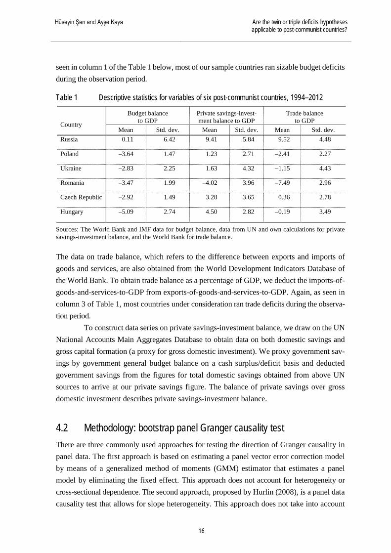
seen in column 1 of the Table 1 below, most of our sample countries ran sizable budget deficits during the observation period. Table 1 Descriptive statistics for variables of six post-communist countries, 1994–2012
Country
Budget balance to GDP
Private savings-invest-ment balance to GDP
Trade balance to GDP
Mean Std. dev. Mean Std. dev. Mean Std. dev. Russia 0.11 6.42 9.41 5.84 9.52 4.48
Poland –3.64 1.47 1.23 2.71 –2.41 2.27
Ukraine –2.83 2.25 1.63 4.32 –1.15 4.43
Romania –3.47 1.99 –4.02 3.96 –7.49 2.96
Czech Republic –2.92 1.49 3.28 3.65 0.36 2.78
Hungary –5.09 2.74 4.50 2.82 –0.19 3.49
Sources: The World Bank and IMF data for budget balance, data from UN and own calculations for private savings-investment balance, and the World Bank for trade balance. The data on trade balance, which refers to the difference between exports and imports of goods and services, are also obtained from the World Development Indicators Database of the World Bank. To obtain trade balance as a percentage of GDP, we deduct the imports-of-goods-and-services-to-GDP from exports-of-goods-and-services-to-GDP. Again, as seen in column 3 of Table 1, most countries under consideration ran trade deficits during the observa-tion period.
To construct data series on private savings-investment balance, we draw on the UN National Accounts Main Aggregates Database to obtain data on both domestic savings and gross capital formation (a proxy for gross domestic investment). We proxy government sav-ings by government general budget balance on a cash surplus/deficit basis and deducted government savings from the figures for total domestic savings obtained from above UN sources to arrive at our private savings figure. The balance of private savings over gross domestic investment describes private savings-investment balance. 4.2 Methodology: bootstrap panel Granger causality test There are three commonly used approaches for testing the direction of Granger causality in panel data. The first approach is based on estimating a panel vector error correction model by means of a generalized method of moments (GMM) estimator that estimates a panel model by eliminating the fixed effect. This approach does not account for heterogeneity or cross-sectional dependence. The second approach, proposed by Hurlin (2008), is a panel data causality test that allows for slope heterogeneity. This approach does not take into account
BOFIT- Institute for Economies in Transition Bank of Finland
BOFIT Discussion Papers 3/ 2016
17
cross-sectional dependence, which, if it exists, creates substantial biases and size distortions. The third approach, proposed by Kónya (2006), allows both heterogeneity and cross-sectional dependence to be taken into account.
This study employs the approach proposed by Konya (2006), which has three ad-vantages over the first two approaches. First, this approach is based on a SUR estimation that allows us take into account cross-sectional dependence across countries. Second, it does not require the joint hypothesis for all members of the panel because it is based on a Wald test with country-specific bootstrap critical values. Finally, it requires no pre-testing for panel unit roots or co-integrating relationships. A general drawback of the unit root test is its low testing power, which can lead to incorrect judgments with regard to co-integrating relation-ships.
Here, we take into account the possible existence of direct relationship between budget deficits and trade deficits, and/or among budget deficits, private savings-investment deficits, and trade deficits. For this purpose, we employ the bootstrap Granger causality ap-proach developed by Kónya (2006), based on bi-variate [budget balance (BB) and private sav-ings-investment balance (SIB)] and tri-variate [(BB), (SIB), and trade balance (NXB)] finite-order vector autoregressive models. In our opinion, the bootstrap panel causality approach is superior to the first two techniques mentioned above in terms of accounting for cross-sectional dependency and country-specific heterogeneity. In detecting Granger causal relation-ships, the bootstrap panel causality approach is based on seemingly unrelated regressions (SUR) estimation of the set of equations and Wald statistics with country-specific bootstrap critical values. Notably, Kónya (2006) indicated that this approach does not require any pre-testing for the panel unit root and cointegration. Since country-specific bootstrap critical values are used, the model variables need not be stationary. The variables can be used in level form regardless of their unit root and cointegration properties.
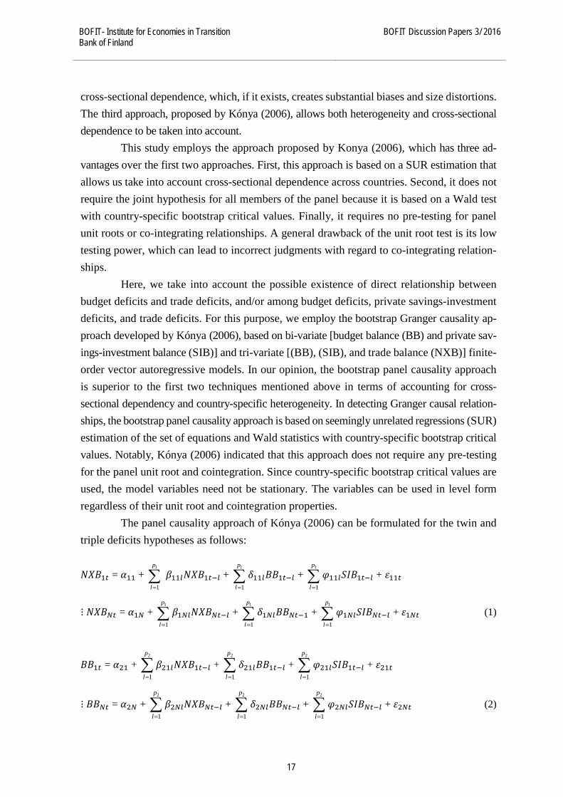
The panel causality approach of Kónya (2006) can be formulated for the twin and triple deficits hypotheses as follows:
𝑁𝑁𝑁𝑁𝑁𝑁1𝑡𝑡 = 𝛼𝛼11 + 1
1
p
l=∑ 𝛽𝛽11𝑙𝑙𝑁𝑁𝑁𝑁𝑁𝑁1𝑡𝑡−𝑙𝑙 +
1
1
p
l=∑ 𝛿𝛿11𝑙𝑙𝑁𝑁𝑁𝑁1𝑡𝑡−𝑙𝑙 +
1
1
p
l=∑ 𝜑𝜑11𝑙𝑙𝑆𝑆𝑆𝑆𝑁𝑁1𝑡𝑡−𝑙𝑙 + 𝜀𝜀11𝑡𝑡
⋮ 𝑁𝑁𝑁𝑁𝑁𝑁𝑁𝑁𝑡𝑡 = 𝛼𝛼1𝑁𝑁 + 1
1
p
l=∑ 𝛽𝛽1𝑁𝑁𝑙𝑙𝑁𝑁𝑁𝑁𝑁𝑁𝑁𝑁𝑡𝑡−𝑙𝑙 +
1
1
p
l=∑ 𝛿𝛿1𝑁𝑁𝑙𝑙𝑁𝑁𝑁𝑁𝑁𝑁𝑡𝑡−1 +
1
1
p
l=∑ 𝜑𝜑1𝑁𝑁𝑙𝑙𝑆𝑆𝑆𝑆𝑁𝑁𝑁𝑁𝑡𝑡−𝑙𝑙 + 𝜀𝜀1𝑁𝑁𝑡𝑡 (1)
𝑁𝑁𝑁𝑁1𝑡𝑡 = 𝛼𝛼21 + 2
1
p
l=∑ 𝛽𝛽21𝑙𝑙𝑁𝑁𝑁𝑁𝑁𝑁1𝑡𝑡−𝑙𝑙 +
2
1
p
l=∑ 𝛿𝛿21𝑙𝑙𝑁𝑁𝑁𝑁1𝑡𝑡−𝑙𝑙 +
2
1
p
l=∑ 𝜑𝜑21𝑙𝑙𝑆𝑆𝑆𝑆𝑁𝑁1𝑡𝑡−𝑙𝑙 + 𝜀𝜀21𝑡𝑡
⋮ 𝑁𝑁𝑁𝑁𝑁𝑁𝑡𝑡 = 𝛼𝛼2𝑁𝑁 + 2
1
p
l=∑ 𝛽𝛽2𝑁𝑁𝑙𝑙𝑁𝑁𝑁𝑁𝑁𝑁𝑁𝑁𝑡𝑡−𝑙𝑙 +
2
1
p
l=∑ 𝛿𝛿2𝑁𝑁𝑙𝑙𝑁𝑁𝑁𝑁𝑁𝑁𝑡𝑡−𝑙𝑙 +
2
1
p
l=∑ 𝜑𝜑2𝑁𝑁𝑙𝑙𝑆𝑆𝑆𝑆𝑁𝑁𝑁𝑁𝑡𝑡−𝑙𝑙 + 𝜀𝜀2𝑁𝑁𝑡𝑡 (2)
Hüseyin Şen and Ayşe Kaya Are the twin or triple deficits hypotheses applicable to post-communist countries?
18
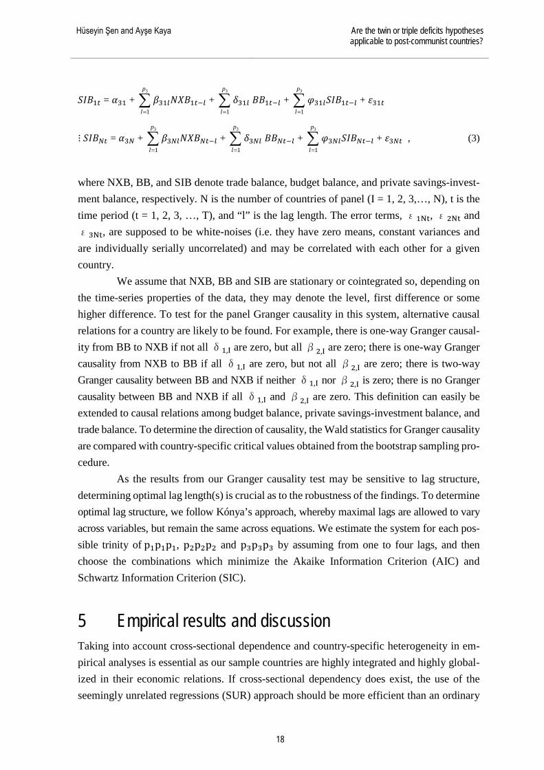
𝑆𝑆𝑆𝑆𝑁𝑁1𝑡𝑡 = 𝛼𝛼31 + 3
1
p
l=∑ 𝛽𝛽31𝑙𝑙𝑁𝑁𝑁𝑁𝑁𝑁1𝑡𝑡−𝑙𝑙 +
3
1
p
l=∑ 𝛿𝛿31𝑙𝑙 𝑁𝑁𝑁𝑁1𝑡𝑡−𝑙𝑙 +
3
1
p
l=∑ 𝜑𝜑31𝑙𝑙𝑆𝑆𝑆𝑆𝑁𝑁1𝑡𝑡−𝑙𝑙 + 𝜀𝜀31𝑡𝑡
⋮ 𝑆𝑆𝑆𝑆𝑁𝑁𝑁𝑁𝑡𝑡 = 𝛼𝛼3𝑁𝑁 + 3
1
p
l=∑ 𝛽𝛽3𝑁𝑁𝑙𝑙𝑁𝑁𝑁𝑁𝑁𝑁𝑁𝑁𝑡𝑡−𝑙𝑙 +
3
1
p
l=∑ 𝛿𝛿3𝑁𝑁𝑙𝑙 𝑁𝑁𝑁𝑁𝑁𝑁𝑡𝑡−𝑙𝑙 +
3
1
p
l=∑ 𝜑𝜑3𝑁𝑁𝑙𝑙𝑆𝑆𝑆𝑆𝑁𝑁𝑁𝑁𝑡𝑡−𝑙𝑙 + 𝜀𝜀3𝑁𝑁𝑡𝑡 , (3)
where NXB, BB, and SIB denote trade balance, budget balance, and private savings-invest-ment balance, respectively. N is the number of countries of panel (I = 1, 2, 3,…, N), t is the time period (t = 1, 2, 3, …, T), and “l” is the lag length. The error terms, ε1Nt, ε2Nt and ε3Nt, are supposed to be white-noises (i.e. they have zero means, constant variances and are individually serially uncorrelated) and may be correlated with each other for a given country.
We assume that NXB, BB and SIB are stationary or cointegrated so, depending on the time-series properties of the data, they may denote the level, first difference or some higher difference. To test for the panel Granger causality in this system, alternative causal relations for a country are likely to be found. For example, there is one-way Granger causal-ity from BB to NXB if not all δ1,I are zero, but all β2,I are zero; there is one-way Granger causality from NXB to BB if all δ1,I are zero, but not all β2,I are zero; there is two-way Granger causality between BB and NXB if neither δ1,I nor β2,I is zero; there is no Granger causality between BB and NXB if all δ1,I and β2,I are zero. This definition can easily be extended to causal relations among budget balance, private savings-investment balance, and trade balance. To determine the direction of causality, the Wald statistics for Granger causality are compared with country-specific critical values obtained from the bootstrap sampling pro-cedure.
As the results from our Granger causality test may be sensitive to lag structure, determining optimal lag length(s) is crucial as to the robustness of the findings. To determine optimal lag structure, we follow Kónya’s approach, whereby maximal lags are allowed to vary across variables, but remain the same across equations. We estimate the system for each pos-sible trinity of p1p1p1, p2p2p2 and p3p3p3 by assuming from one to four lags, and then choose the combinations which minimize the Akaike Information Criterion (AIC) and Schwartz Information Criterion (SIC).
5 Empirical results and discussion Taking into account cross-sectional dependence and country-specific heterogeneity in em-pirical analyses is essential as our sample countries are highly integrated and highly global-ized in their economic relations. If cross-sectional dependency does exist, the use of the seemingly unrelated regressions (SUR) approach should be more efficient than an ordinary
BOFIT- Institute for Economies in Transition Bank of Finland
BOFIT Discussion Papers 3/ 2016
19
least-squares (OLS) approach in estimating panel data causality. Moreover, the causality re-sults obtained from the SUR estimator developed by Zellner (1962) should be more reliable than those obtained from county-specific OLS estimations. The Monte Carlo experiment by Pesaran (2006) emphasizes the importance of testing for the cross-sectional dependence in a panel data study. It also illustrates the substantial bias and size distortions that arise when cross-sectional dependence is ignored.
A further issue to decide is whether to treat slope coefficients as homogenous to impose the causality restriction on the estimated parameters. The causality from one variable to another variable by imposing the joint restriction for the panel is the strong null hypothesis and the homogeneity assumption for the parameters is unable to capture heterogeneity due to country-specific characteristics.
Thus, we start our empirical analysis with testing for cross-sectional dependency, followed by slope homogeneity across countries. We then select the appropriate panel cau-sality method for determining the direction of causality between budget balance, private sav-ings-investment balance, and trade balance in our six post-communist countries.
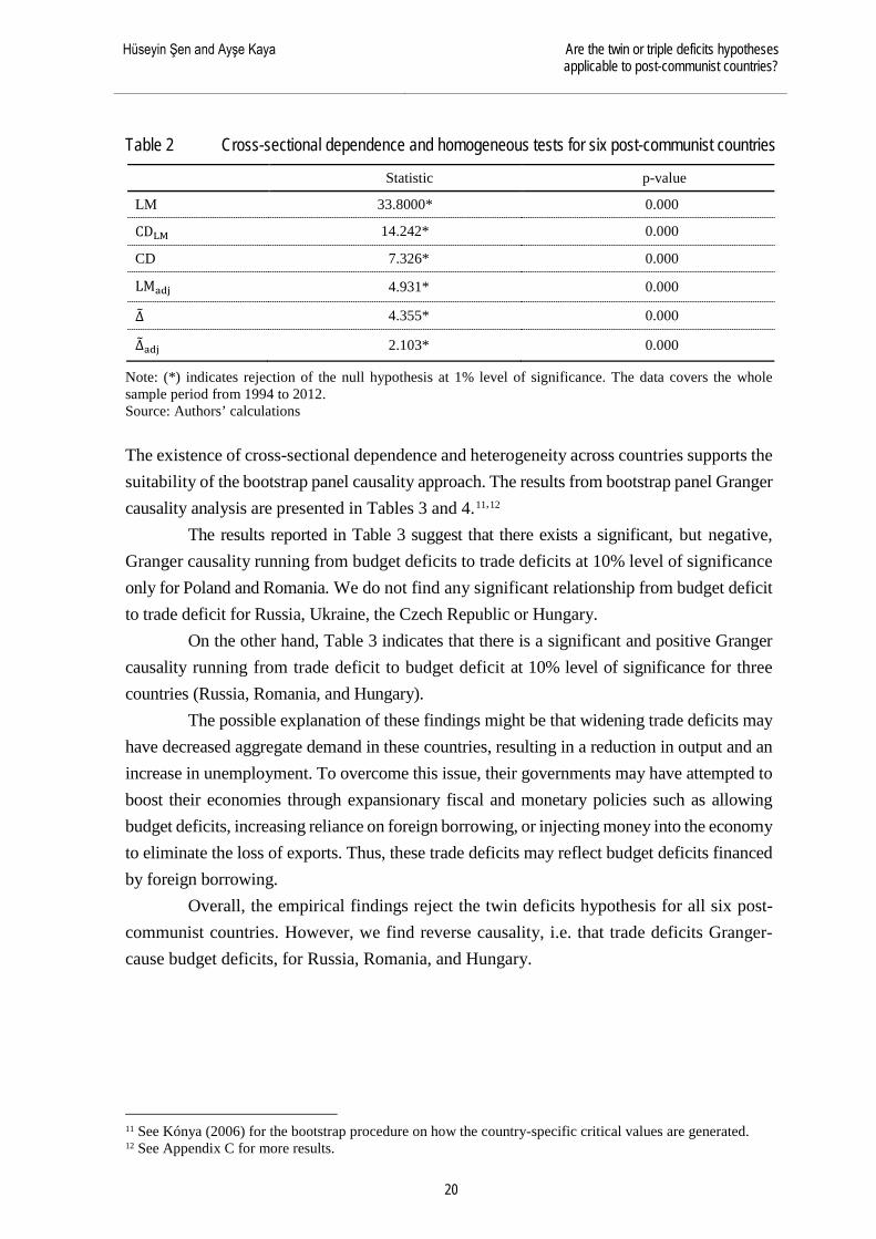
To investigate the existence of cross-sectional dependence, we implement four tests: the LM, CDlm, CD and LMadj tests.9 The test results are presented below in Table 2. As shown from the table, the null hypothesis of no cross-sectional dependence across the coun-tries is strongly rejected at 1% level of significance, implying that the SUR method is more appropriate than country-by-country OLS estimation. The findings in Table 2 indicate that a shock in one sample country is transmitted to the other countries under consideration. The same table also reports the results of two slope homogeneity tests (∆� , ∆�𝑎𝑎𝑎𝑎𝑎𝑎).10 The test findings of both tests reject the null hypothesis of slope homogeneity for each group of countries, thus supporting country-specific heterogeneity. The rejection of slope homogeneity implies that the panel causality analysis imposing homogeneity restriction on the variable of interest results in misleading inferences.
9 See Appendix B for a detailed description of the cross-sectional dependence tests. 10 See Appendix B for details of the slope homogeneity tests.
Hüseyin Şen and Ayşe Kaya Are the twin or triple deficits hypotheses applicable to post-communist countries?
20
Table 2 Cross-sectional dependence and homogeneous tests for six post-communist countries
Statistic p-value
LM 33.8000* 0.000
CDLM 14.242* 0.000
CD 7.326* 0.000
LMadj 4.931* 0.000
∆� 4.355* 0.000
∆�adj 2.103* 0.000
Note: (*) indicates rejection of the null hypothesis at 1% level of significance. The data covers the whole sample period from 1994 to 2012. Source: Authors’ calculations The existence of cross-sectional dependence and heterogeneity across countries supports the suitability of the bootstrap panel causality approach. The results from bootstrap panel Granger causality analysis are presented in Tables 3 and 4.11,12
The results reported in Table 3 suggest that there exists a significant, but negative, Granger causality running from budget deficits to trade deficits at 10% level of significance only for Poland and Romania. We do not find any significant relationship from budget deficit to trade deficit for Russia, Ukraine, the Czech Republic or Hungary.
On the other hand, Table 3 indicates that there is a significant and positive Granger causality running from trade deficit to budget deficit at 10% level of significance for three countries (Russia, Romania, and Hungary).
The possible explanation of these findings might be that widening trade deficits may have decreased aggregate demand in these countries, resulting in a reduction in output and an increase in unemployment. To overcome this issue, their governments may have attempted to boost their economies through expansionary fiscal and monetary policies such as allowing budget deficits, increasing reliance on foreign borrowing, or injecting money into the economy to eliminate the loss of exports. Thus, these trade deficits may reflect budget deficits financed by foreign borrowing.
Overall, the empirical findings reject the twin deficits hypothesis for all six post-communist countries. However, we find reverse causality, i.e. that trade deficits Granger-cause budget deficits, for Russia, Romania, and Hungary.
11 See Kónya (2006) for the bootstrap procedure on how the country-specific critical values are generated. 12 See Appendix C for more results.

BOFIT- Institute for Economies in Transition Bank of Finland
BOFIT Discussion Papers 3/ 2016
21
Table 3 Panel Granger causality between budget balance (BB) and trade balance (NXB)
Country
Estimated coefficient
Wald test
Bootstrap critical values Granger causality
Yes/No 10% 5% 1%
𝐇𝐇𝟎𝟎 : Budget deficits do not cause trade deficits
Russia –0.01338 0.42347 7.47146 10.48650 18.09132 No
Poland –0.40196 8.43258*** 6.15855 10.14831 19.55460 Yes
Ukraine 0.23545 0.97061 6.65941 9.95018 16.42223 No
Romania –0.92404 20.20951*** 7.25294 11.68645 22.02894 Yes
Czech Republic
–0.13205 0.42753 6.50894 9.31977 18.09772 No
Hungary 0.15658 1.90532 5.93777 9.32404 17.52335 No
𝐇𝐇𝟎𝟎 : Trade deficits do not cause budget deficits
Russia 0.76100 11.36284*** 6.98460 10.02295 17.03960 Yes
Poland 0.17234 3.26816 7.34377 10.49350 20.58291 No
Ukraine 0.21855 6.33932 6.90682 9.83193 21.95872 No
Romania 0.16497 6.87736*** 6.84733 10.70928 16.54435 Yes
Czech Republic
–0.023962 0.35011 7.60660 11.41818 20.16391 No
Hungary 0.63851 9.06185*** 7.46853 10.96797 18.97539 Yes
Note: The data covers the whole sample period from 1994 to 2012. (***) indicates statistical significance at 10%. Source: Authors’ calculations The results of our tri-variate model where NXB is the independent variable, BB and SIB are the dependent variables are reported in Table 4. As the table shows, the bootstrap critical values considerably higher than the chi-square critical values usually applied with the Wald test, and that they vary considerably from country to country. The Granger causality test results for the null hypothesis show that BB and SIB do not Granger cause NXB as indicated in the Wald test column of Table 4. In other words, the null hypothesis of non-causality is accepted for all the countries under consideration. We do not find empirical support for the validity of triple deficits hypothesis for these countries.

Hüseyin Şen and Ayşe Kaya Are the twin or triple deficits hypotheses applicable to post-communist countries?
22
Table 4 Panel Granger causality from budget balance (BB) and private savings-investment balance (SIB) to trade balance (NXB)
Country
Estimated coefficient
Wald test
Bootstrap critical values
Granger causality
Yes/No
10% 5% 1%
𝐇𝐇𝟎𝟎 : Budget deficits and savings-investment deficits do not cause trade deficits
Russia –17.78857 0.81986 9.40823 16.11821 54.14434 No
Poland 93.97035 3.83792 6.48852 8.13023 12.97103 No
Ukraine 14.07559 4.66484 8.36666 10.91874 18.57224 No
Romania 225.71975 3.48975 11.06174 13.79216 23.27718 No
Czech Republic
–24.59393 0.10745 7.73098 9.13379 17.55371 No
Hungary –160.52930 4.81681 5.23574 8.89057 20.13321 No
Note: The data cover the whole sample period from 1994 to 2012. Source: Authors’ calculations Overall, Table 5 summarizes our results of the direction of panel Granger causality among the three variables for all the countries examined. As can be seen from the table, the empir-ical results do not support the validity of the twin or triple deficits hypotheses for any of our sample countries. Specifically, their budget deficits do not Granger-cause trade deficits and the existence of dual domestic deficits (budget plus savings-investment deficits) does not lead to external deficits.

BOFIT- Institute for Economies in Transition Bank of Finland
BOFIT Discussion Papers 3/ 2016
23
Table 5 Direction of panel Granger causality for post-communist countries Possible direction of Granger causality Country Granger causality exists
BB ⟶ NXB
Poland and Romania Yes Significant and negative
Russia, Ukraine, Czech Republic, and Hungary No Insignificant
NXB ⟶ BB Russia, Romania, and Hungary Yes Significant and positive
Poland, Ukraine, and Czech Republic No Insignificant
BB ⟶ SIB
Poland and Romania Yes Significant and negative
Russia, Ukraine, Czech Republic, and Hungary
No Insignificant
SIB ⟶ BB Russia, Ukraine, and Hungary Yes Significant and positive
Poland, Romania, and Czech Republic No Insignificant
SIB ⟶ NXB
Poland and Romania Yes Significant and positive
Russia, Ukraine, Czech Republic, and Hungary
No Insignificant
NXB ⟶ SIB
Poland and Romania Yes Significant and negative
Russia, Ukraine, Czech Republic, and Hungary
No Insignificant
BB, SIB ⟶ NXB Russia, Poland, Ukraine, Romania, Czech Republic, and Hungary No Insignificant
Notes: BB, SIB, NX denote budget balance, private savings-investment balance, and trade balance, respec-tively. “→” represents Granger causal direction. Source: Authors’ summary
6 Concluding remarks In this study, we tested for evidence of the twin and triple deficits hypotheses in six post-communist countries (Russia, Poland, Ukraine, Romania, the Czech Republic, and Hungary) over the period 1994–2012. We first examined the existence of possible Granger causalities between budget and trade balance, and then tri-variate Granger causalities among the budget balance, private savings-investment balance, and trade balance. Our analysis was based on the bootstrap panel Granger causality technique, which allows us to capture cross-sectional de-pendence and heterogeneity across countries.
We find no evidence in favor of the twin/triple deficits hypothesis for the countries considered. This means that there is no Granger causality running from budget deficits to trade deficits, and no Granger causality was found running from budget deficits and private

Hüseyin Şen and Ayşe Kaya Are the twin or triple deficits hypotheses applicable to post-communist countries?
24
savings-investment deficits to trade deficits. Based on these findings, we conclude that the Ricardian equivalence proposition of the twin and triple deficits hypotheses holds for these six post-communist countries over the observation period.
Overall, it appears that budget deficits and trade deficits are causally independent var-iables in our sample. It is worth mentioning that our findings are broadly parallel to the empir-ical findings of several earlier studies, including Dewald and Ulan (1990) and Rahmann and Mishra (1992) for the US, Kaufmann et al. (2002) for Austria, Abbas et al. (2010) for 124 coun-tries, Kıran (2011) for Turkey, and Ogbonna (2014) for South Africa. Further, our findings are consistent with all but a limited number of studies on post-communist transitions countries, specifically Gurgul and Lach (2012), Aristovnik and Djurić (2013), and Gabrisch (2015).
There may be several explanations for these findings. First, the existence of an out-put gap may be a factor. With some minor exceptions, all sample countries in the first decade of the transition displayed actual output levels in proportion to potential GDP well below their potential levels. This suggests the existence of an output gap. If so, increases in aggregate demand following expansionary fiscal policies may have been masked by increases in do-mestically produced goods and services, rather than through imports. The second plausible explanation may be a substantial exogenous increase in investment. These investment booms might have been generated through foreign technical assistance, technological innovation, successful market-oriented reforms, or a combination of all three. Successfully implemented free-market reforms, in particular, would have conferred the economic benefits of growth, en-hanced trade competitiveness, and inflows of much-needed foreign capital. Third, there was the external assistance these countries received at the earlier stages of transition from interna-tional financial organizations such as the IMF, World Bank, as well as bilateral donors. More-over, the countries that have already joined the EU all received substantial financial and tech-nical supports from the EU throughout their accession processes. Finally, Russia and Ukraine are commodity-exporting countries13 and so their export earnings and demand de-pend mostly on external factors. Over the observation period, there were several currency devaluations that effectively restrained imports to Russia and Ukraine.
This study broadly relates to possible explanations for the divergent results among the many empirical papers. The different findings may largely arise from the differences in methodology and data. In some previous studies, the possibility of structural breaks was ignored in the series. In others, the variables considered were treated as integrated of order “one”, referring to the existence of a unit root. Further, analysis of data sets that focus on a short period of time may not yield reliable evidence. Lack of longer-term data for countries, as in the case of this study, limits the possibility for clear-cut, differentiated results. Not to put a fine point on
13 Both are resource-rich countries, with iron and steel playing particularly large export roles. For Russia, of course, oil and oil- related products are dominant export products.
BOFIT- Institute for Economies in Transition Bank of Finland
BOFIT Discussion Papers 3/ 2016
25
it, but differences in econometric techniques, data measures, samples employed, etc. yield dif-ferent results. To overcome such differences, future studies should concentrate on compari-son of various estimation techniques on a common data set. The same holds for country-specific features. Country-specific features such as exchange rate regime differences, deficit financing strategies, economy structure, institutional arrangements, etc. similarly affect the findings of various papers.
All in all, based on our empirical findings, it could be argued that if the Ricardian proposition holds true, fiscal policy is limited in its ability to influence trade (or current account) deficits. From a policy standpoint, such an evidence implies that the causes of large and persistent external deficits must be sought somewhere else than the budget side of the economy. Behind this, there might be several reasons, such as the structure of foreign trade, the exchange rate regime pursued, and the international competitiveness of the particular country in question, the degree of capital mobility, and the Feldstein-Horioka puzzle. Nev-ertheless, it is obvious that the case for the twin or triple deficits hypotheses is more likely to be seen in countries with economies that are highly integrated with international markets, open to capital movements, and experience intensive international competitiveness.

Hüseyin Şen and Ayşe Kaya Are the twin or triple deficits hypotheses applicable to post-communist countries?
26
References Abbas, M. S. A., Bouhga-Hagbe, J., Fatás, A. J., Mauro, P., and Velloso, R. C. (2010), “Fis-
cal Policy and Current Account,” IMF Working Paper, WP/10/121, 31.
Abell, J. (1990), “Twin Deficits during the 1980s: An Empirical Investigation,” Journal of Mac-roeconomics, 12 (1), 81–96.
Afonso, A., Rault, C., and Estay, C. (2013), “Budgetary and External Imbalances Relationship: A Panel Data Diagnostic,” Journal of Quantitative Economics, 11 (1 and 2 com-bined), 84–110.
Ahmed, S. M. and Ansari, M. I. (1994), “A Tale of Two Deficits: An Empirical Investigation for Canada,” International Trade Journal, 8 (4), 483–503.
Ahmad, A. H., Aworinde, O. B. and Martin, C. (2015), “Threshold Cointegration and the Short-Run Dynamics of Twin Deficits Hypothesis in African Countries” Journal of Eco-nomic Asymmetries, 12, 80–91.
Akıncı, M. and Yılmaz, Ö. (2012), “Validity of the Triple Deficit Hypothesis in Turkey: Bounds Test Approach,” Istanbul Stock Exchange Review, 13 (50), 1–28.
Aristovnik, A. and Djurić, S. (2013), “Twin Deficits and the Feldstein-Horioka Puzzle: A Com-parison of the EU Member States and Candidate Countries,” Actual Problems of Eco-nomics, 143 (5), 205–214.
Anoruo, E. and Ramchander, S. (1998), “Current Account and Fiscal Deficits: Evidence from Five Developing Economies of Asia,” Journal of Asian Economics, 9 (3), 487–501.
Asrafuzzaman, A., Roy, A., and Gupta, S. D. (2013), “An Empirical Investigation of Budget and Trade Deficits: The Case of Bangladesh,” International Journal of Economics and Financial Issues, 3 (3), 570–579.
Baharumshah, A. Z., Lau, E. and Khalid, A. M. (2006), “Testing Twin Deficits Hypothesis using VARs and Variance Decomposition,” Journal of the Asia Pacific Economy, 11 (3), 331–354.
Baharumshah, A. Z. and Lau, E. (2007), “Dynamics of Fiscal and Current Account Deficits in Thailand: An Empirical Investigation,” Journal of Economic Studies, 34 (6), 454–475.
Barro, R. J. (1974), “Are Government Bonds Net Wealth?” Journal of Political Economy, 82 (6), 1095–1117.
Barro, R. J. (1989), “The Ricardian Approach to Budget Deficits,” Journal of Economic Per-spectives, 3 (2), 37–54.
Bernheim, B. D. (1988), “Budget Deficits and the Balance of Trade,” in Lawrence H. Sum-mers (ed.), Tax Policy and the Economy, MIT Press: Cambridge, 1–32.
Bostancı, E. and Tunç, G. İ. (2002), “Turkish Twin Deficits: An Error Correction Model of Trade Balance,” METU ERC Working Papers in Economics, No. 01/06, May 2002.
Breusch, T. and Pagan, A. (1980), “The Lagrange Multiplier Test and Its Application to Model Specifications in Econometrics,” Reviews of Economics Studies, 47, 239–253.
Dewald, W. G. and Ulan, M. (1990), “The Twin-Deficit Illusion,” Cato Journal, 9 (3), 689–707.

BOFIT- Institute for Economies in Transition Bank of Finland
BOFIT Discussion Papers 3/ 2016
27
Eldemerdash, H., Metcalf, H. and Maioli, S. (2014), “Twin Deficits: New Evidence from a De-veloping (Oil vs. Non-Oil) Countries’ Perspective,” Empirical Economics, 47, 825–851.
El-Baz, O. (2014), “Empirical Investigation of the Twin Deficits Hypothesis: The Egyptian Case (1990–2012),” Munich Personal RePEc Archive, MPRA Paper No. 53428, 25.
Enders, W. and Lee, B-S. (1990), “Current Account and Budget Deficits: Twins or Distant Cous-ins?” Review of Economics and Statistics, 72 (3), 373–381.
Feldstein, M. (1992), “The Budget and Trade Deficits Aren’t Really Twins,” Challenge, 35 (2), 60–63.
Fidrmuc, J. (2003), “The Feldstein-Horioka Puzzle and Twin Deficits in Selected Countries,” Economics of Planning, 36 (2), 135–152.
Frankel, J. A. (2006), “Twin Deficits and Twin Decades,” in Richard W. Kopcke, Geoffrey M. B. Tootell, and Robert K. Triest (eds.), The Macroeconomics of Fiscal Policy, MIT Press: Cambridge, Massachusetts, London, England, 321–335.
Gabrisch, H. (2015), “On the Twin Deficits Hypothesis and the Import Intensity in Transition Countries,” International Economics and Economic Policy, 12 (2), 205–220.
Gurgul, H. and Lach, L. (2012), “Two Deficits and Economic Growth: Case of CEE Countries in Transition,” Managerial Economics, 12, 79–108.
Holmes, M. J. (2010), “A Reassessment of the Twin Deficits Relationship,” Applied Economics Letters, 17, 1209–1212.
Hurlin, C. (2008), “Testing for Granger Non Causality in Heterogeneous Panels,” mimeo, De-partment of Economics: University of Orleans.
IMF (2000), “Transition: Experiences and Policy Issues,” in World Economic Outlook: Focus on Transition Economies, October 2000, Chapter 3, International Monetary Fund: Wash-ington D.C., 84–137.
IMF (2011), “Separated at Birth? The Twin Budget and Trade Balances,” in World Economic Outlook: Slowing Growth, Rising Risks, September 2011, Chapter 4, International Mon-etary Fund: Washington DC., 135–160.
IMF (2014), “25 Years of Transition Post-Communist Europe and the IMF,” Special Report: Regional Economic Issues, International Monetary Fund, 62.
Islam, M. F. (1998), “Brazil’s Twin Deficits: An Empirical Investigation,” Atlantic Eco-nomic Journal, 26 (2), 121–128.
Kaufmann, S., Scharler, J., and Winckler, G. (2002), “The Austrian Current Account: Driven by Twin Deficits and by Intertemporal Expenditure Allocation?” Empirical Economics, 27, 529–542.
Kiran, B. (2011), “On the Twin Deficits Hypothesis: Evidence from Turkey,” Applied Econ-ometrics and International Development, 11–1, 59–66.
Kim, C-H. and Kim, D. (2006), “Does Korea Have Twin Deficits?” Applied Economics Letters, 13, 675–680.
Kim, S. and Roubini, N. (2008), “Twin Deficit or Twin Divergence? Fiscal Policy, Current Ac-count, and Real Exchange Rate in the U.S.,” Journal of International Economics, 74, 362–383.
Hüseyin Şen and Ayşe Kaya Are the twin or triple deficits hypotheses applicable to post-communist countries?
28
Kalou, S. and Paleologou, S-M. (2012), “The Twin Deficits Hypothesis: Revisiting an EMU Country,” Journal of Policy Modeling, 34, 230–241.
Khalid, A. M. and Guan, T. W. (1999), “Causality Tests of Budget and Current Account Deficits: Cross-Country Comparisons,” Empirical Economics, 24, 389–402.
Kónya, L. (2006), “Exports and Growth: Granger Causality Analysis on OECD Countries with a Panel Data Approach,” Economic Modelling, 23, 978–992.
Latif-Zaman, N. and DaCosta, M. N. (1990), “The Budget Deficits and the Trade Deficit: Insights Into This Relationship,” Eastern Economic Journal, 16 (4), 349–354.
Lau, E., Mansor, S. A., and Puah, C-H. (2010), “Revival of the Twin Deficits in Asian Crisis-affected Countries,” Economic Issues, 15 (1), 29–53.
Magazzino, C. (2012), “The Twin Deficits Phenomenon: Evidence from Italy,” Journal of Eco-nomic Cooperation and Development, 33 (3), 65–80.
Mankiw, N. G. (2006), “Reflections on the Trade Deficit and Fiscal Policy,” Journal of Policy Modeling, 28, 679–682.
Marinheiro, C. F. (2008), “Ricardian Equivalence, Twin Deficits, and the Feldstein-Horioka Puzzle in Egypt,” Journal of Policy Modeling, 30 (6), 1041–1056.
Miller, S. and Russek, F. S. (1989), “Are the Twin Deficits Really Related?” Contemporary Economic Policy, 7 (4), 91–115.
Milne, E. (1977), “The Fiscal Approach to the Balance of Payments,” Economic Notes, 6, 889–908.
Mudassar, K., Fakher, A., Ali, S. and Sarwar, F. (2013), “Validation of Twin Deficits Hypothe-sis: A Case Study of Pakistan,” Universal Journal of Management and Social Sci-ences, 3 (10), 33–47.
Normandin, M. (1999), “Budget Deficit Persistence and the Twin Deficits Hypothesis,” Journal of International Economics, 49, 171–193.
Ogbonna, B. C. (2014), “Investigating for Twin Deficits Hypothesis in South Africa,” Develop-ing Country Studies, 4 (10), 142–162.
Pesaran, M.H. (2004), “General Diagnostic Tests for Cross Section Dependence in Panels,” CE-Sifo Working Paper No. 1229 (IZA Discussion Paper No. 1240).
Pesaran, M. H. (2006), “Estimation and Inference in Large Heterogeneous Panel with a Mul-tifactor Error Structure,” Econometrica, 74 (4), 967–1012.
Pesaran, M. H., Ullah, A., and Yamagata, T. (2008), “A Bias-Adjusted LM Test of Error Crosssection Independence,” Econometrics Journal, 11 (1), 105–127.
Pesaran, M. H. and Yamagata, T. (2008), “Testing Slope Homogeneity in Large Panels,” Journal of Econometrics, 142 (1), 50–93.
Rahman, M. and Mishra, B. (1992), “Cointegration of US Budget and Current Account Deficits: Twins or Strangers?” Journal of Economics and Finance, 16 (2), 119–127.
Ratha, A. (2012), “Twin Deficits or Distant Cousins?: Evidence from India,” South Asia Eco-nomic Journal, 13 (1), 51–68.
Rosensweig, J. A. and Tallman, E. W. (1993), “Fiscal Policy and Trade Adjustment: Are the Deficits Really Twins?,” Economic Inquary, XXXI, 580–594.
BOFIT- Institute for Economies in Transition Bank of Finland
BOFIT Discussion Papers 3/ 2016
29
Salvatore, D. (2006), “Twin Deficits in the G-7 Countries and Global Structural Imbal-ances,” Journal of Policy Modeling, 28, 701–712.
Swamy, P. A.V. B. (1970), “Efficient Inference in a Random Coefficient Regression Model,” Econometrica, 38 (2), 311–323.
Saleh, A. S., Nair, M. and Agagewatte, T. (2005), “The Twin Deficits Problem in Sri Lanka: An Econometric Analysis,” South Asia Economic Journal, 6 (2), 221–239.
Sobrino, C. R. (2013), “The Twin Deficits Hypothesis and Reverse Causality: A Short-Run Analysis of Peru,” Journal of Economics, Finance and Administrative Science, 18 (34), 9–15.
Szakolczai, G. (2006), “The Triple Deficit of Hungary,” Hungarian Statistical Review, 10, 41.
Şen, A., Şentürk, M., Sancar, C., and Akbaş, Y. E. (2014), “Empirical Findings on Triplet Def-icits Hypothesis: The Case of Turkey,” Journal of Economic Cooperation and Develop-ment, 35 (1), 81–102.
Şen, H., Kaya, A., and Alpaslan, B. (2015), “Education, Health, and Economic Growth Nexus: A Bootstrap Panel Granger Causality Analysis for Developing Countries,” Econom-ics Discussion Paper Series, EDP-1502, University of Manchester, Manchester, UK.
Tang, T. C. (2014), “Fiscal Deficit, Trade Deficit, and Financial Account Deficit: Triple Deficits Hypothesis with the U.S. Experience,” Monash Economics Working Papers from Monash University, Department of Economics, No. 06–14, 13.
Trachanas, E. and Katrakilidis, C. (2013), “The Dynamic Linkages of Fiscal and Current Ac-count Deficits: New Evidence from Five Highly Indebted European Countries Account-ing for Regime Shifts and Asymmetries,” Economic Modelling, 31, 502–510.
Tosun, U., İyidoğan-Varol, P., and Telatar, E. (2014), “The Twin Deficits in Selected Central and Eastern European Economies: Bounds Testing Approach with Causality Analysis,” Romanian Journal of Economic Forecasting, 17 (2), 141–160.
UNECE (2001), “Economic Growth and Foreign Direct Investment in the Transition Econ-omies,” in Economic Survey of Europe, Report by The United Nations Economic Commissions for Europe, No. 1, Chapter 5, pp. 185–225.
Vamvoukas, G. A. (1997), “Have Large Budget Deficits Caused Increasing Trade Deficits? Ev-idence from a Developing Country,” Atlantic Economic Journal, 25 (1), 80–90.
Vamvoukas, G. A. (2010), “The Twin Deficits Phenomenon: Evidence from Greece,” Applied Economics, 31, 1093–1100.
Xie, Z. and Chen, S-W. (2014), “Untangling the Causal Relationship between Government Budget and Current Account Deficits in OECD Countries: Evidence from Bootstrap Panel Granger Causality,” International Review of Economics and Finance, 31, 95–104.
Zellner, A. (1962), “An Efficient Method of Estimating Seemingly Unrelated Regressions and Tests for Aggregation Bias,” Journal of the American Statistical Association, 57, 348–368

Hüseyin Şen and Ayşe Kaya Are the twin or triple deficits hypotheses applicable to post-communist countries?
30
Appendix A Selected empirical studies on twin and triple deficits hypotheses*, 1988–2015
Empirical study Period and country specification
Method or/and model Empirical findings Period Country
Trip
le d
efic
its
hypo
thes
is
Tang (2014) 1960:Q1–2013:Q1 US Autoregressive distributed lag (ARLD) model
US data supports triple-deficits link, i.e. fiscal, current account, and capital and financial account balances move together over the long run.
Şen et al. (2014) 1980–2010 Turkey Dolado-Lütkepohl Granger causality analysis and VAR model
Triple deficits hypothesis valid for Turkey.
Akıncı and Yılmaz (2012)
1975–2010 Turkey Bounds testing approach
Budget and saving deficits positively and significantly affect current account deficits over the short and long run. Triple deficits hypothesis valid for Turkey.
←
Tw
in d
efic
its h
ypot
hesi
s
Gabrisch (2015) 1995: Q1–2010:Q4 Three post-transition countries: Poland, Czech Republic, and Hungary.
Cointegration and VECM for Poland; Granger causality test for the Czech Republic and Hungary
Twin deficits hypothesis rejected.
Ahmad et al. (2015) 1980–2009 Nine African countries: Botswana, Cameroon, Egypt, Morocco, Nigeria, Tanzania, Ethiopia, Kenya, and Uganda.
Threshold cointegration technique Positive cointegrating relationship between fiscal balance and current account balance for six of the nine countries considered (Botswana, Cameroon, Egypt, Morocco, Nigeria, and Tanzania). For Ethiopia, Kenya, and Uganda, a negative cointegrating relationship is found between the fiscal balance and current account balance.
BOFIT- Institute for Economies in Transition Bank of Finland
BOFIT Discussion Papers 3/ 2016
31
Eldemerdash et al. (2014)
1970–2010 Group of Arab countries: Bahrain, Egypt, Jordan, Kuwait, Morocco, Oman, Qatar, Saudi Arabia, Syria, Tunisia, and United Arab Emirates.
Panel data Granger causality test
Positive relationship between fiscal and external balances for oil-producing countries, but no such relationship for non-oil countries. Findings support conventional view for oil-producing countries only. Accordingly, a 1% increase in the ratio of government fiscal balance (surplus/deficit) to GDP tends to (improve/deteriorate) the current account balance to GDP by 0.44–0.89% in oil-producing countries.
El-Baz (2014) 1990–2012 Egypt Granger causality test and vector error correction model (VECM)
Reverse causal relationship between budget deficit and current account deficit that runs from current account deficit to budget deficit.
Ogbonna (2014) 1960–2012 South Africa Bi-variate and multi-variate (VAR) models based on cointegration analysis and the error correction model (ECM).
No evidence of the twin deficits hypothesis over the short run. Findings suggest that the Ricardian equivalence proposition holds for South Africa within a short time horizon.
Xie and Chen (2014) 1980–2010 Eleven OECD countries: Belgium, France, Finland, Greece, Iceland, Ireland, Norway, Spain, Sweden, UK, and Switzerland.
Bootstrap panel Granger causality
Bi-directional causality between the current account deficit and the government budget deficit for all countries studied. Twin deficits hypothesis supported through Keynesian hypothesis or current account targeting hypothesis.
Aristovnik and Djurić (2013)
1995–2008 Twelve new EU members and three candidate countries.
Dynamic panel data model Budget deficits of EU members and candidate countries signal relatively high levels of substitutability between private and public saving, implying a low correlation between fiscal and external imbalances. Empirical results usually reject the validity of the twin deficits hypothesis.
Asrafuzzaman et al. (2013)
1972–2012 Bangladesh VAR and Granger causality test
Bi-directional Granger causality between budget deficit and trade deficit in short run, but no relationship over long run.
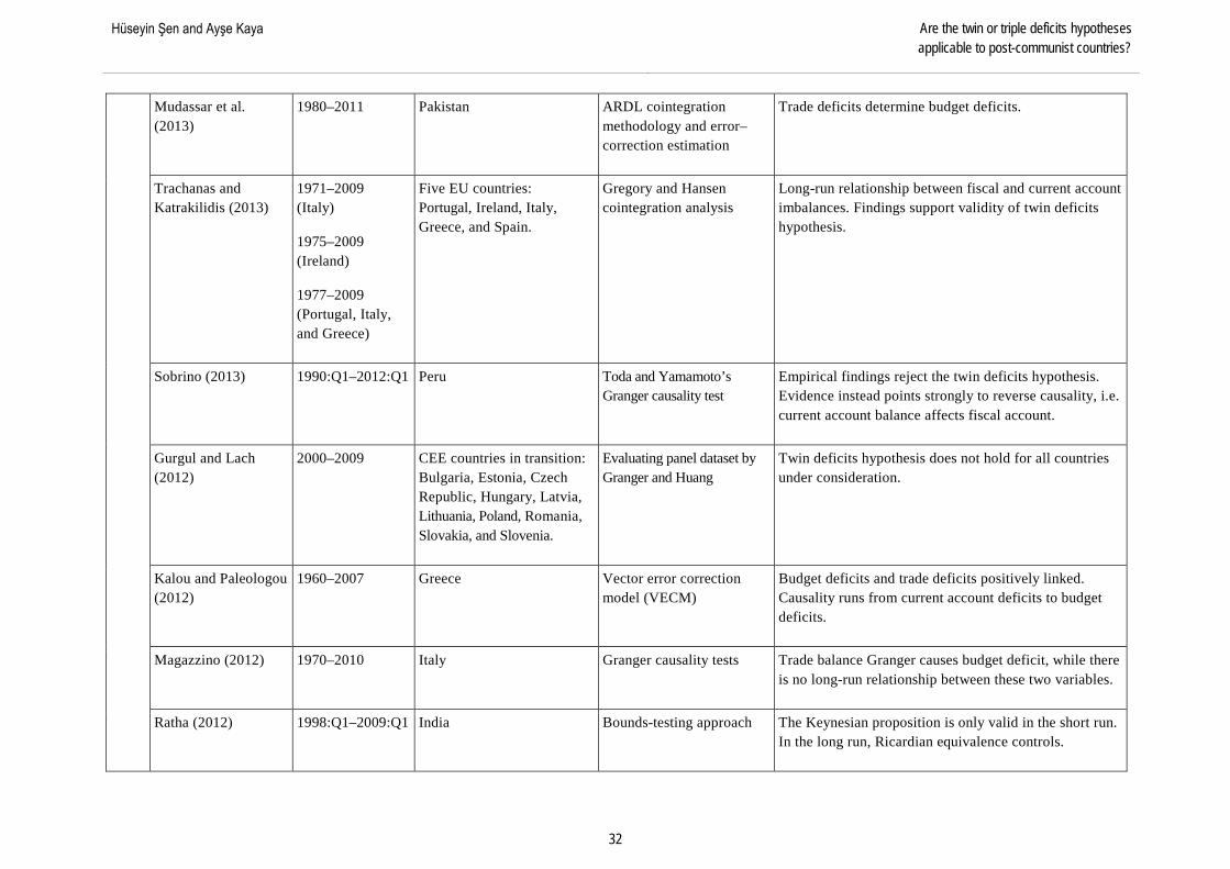
Hüseyin Şen and Ayşe Kaya Are the twin or triple deficits hypotheses applicable to post-communist countries?
32
Mudassar et al. (2013)
1980–2011 Pakistan ARDL cointegration methodology and error–correction estimation
Trade deficits determine budget deficits.
Trachanas and Katrakilidis (2013)
1971–2009 (Italy)
1975–2009 (Ireland)
1977–2009 (Portugal, Italy, and Greece)
Five EU countries: Portugal, Ireland, Italy, Greece, and Spain.
Gregory and Hansen cointegration analysis
Long-run relationship between fiscal and current account imbalances. Findings support validity of twin deficits hypothesis.
Sobrino (2013) 1990:Q1–2012:Q1 Peru Toda and Yamamoto’s Granger causality test
Empirical findings reject the twin deficits hypothesis. Evidence instead points strongly to reverse causality, i.e. current account balance affects fiscal account.
Gurgul and Lach (2012)
2000–2009 CEE countries in transition: Bulgaria, Estonia, Czech Republic, Hungary, Latvia, Lithuania, Poland, Romania, Slovakia, and Slovenia.
Evaluating panel dataset by Granger and Huang
Twin deficits hypothesis does not hold for all countries under consideration.
Kalou and Paleologou (2012)
1960–2007 Greece Vector error correction model (VECM)
Budget deficits and trade deficits positively linked. Causality runs from current account deficits to budget deficits.
Magazzino (2012) 1970–2010 Italy Granger causality tests Trade balance Granger causes budget deficit, while there is no long-run relationship between these two variables.
Ratha (2012) 1998:Q1–2009:Q1 India Bounds-testing approach The Keynesian proposition is only valid in the short run. In the long run, Ricardian equivalence controls.

BOFIT- Institute for Economies in Transition Bank of Finland
BOFIT Discussion Papers 3/ 2016
33
Abbas et al. (2010) 1985–2007 124 countries Panel regressions and panel VARs
The association between fiscal balance and current account balance is limited. Accordingly, an improvement in the fiscal balance of 1% of GDP is found to improve the current account balance by 0.2–0.3 percentage point of GDP. The association between the two is as strong in emerging and low-income economies as in advanced countries; significantly stronger in country-years where output is above potential than in cases where below potential.
Kıran (2011) 1975–2009 Turkey Fractional cointegration approach
Weak evidence for validity of twin deficit hypothesis. In other word; little evidence to suggest the presence of fractional cointegration relationship between the budget deficit and trade deficit.
Lau et al. (2010) 1976:Q1–1997:Q2 (Pre-crisis period)
and 1997:Q3–2008:Q1 (Post-crisis period)
Five countries hit by the Asian crisis: Malaysia, Indonesia, Korea, Philippines, and Thailand.
Standard time series estimation
Causality runs from budget deficit to current account deficit for Malaysia, the Philippines (pre-crisis), and Thailand, which fits well with the Keynesian view. For Indonesia and Korea, causality runs in the opposite direction. A bi-directional causality exists for the Philippines in the post-crisis era.
Vamvoukas (2010) 1948–1993 Greece Cointegration analysis, error-correction model, and Granger tri-variate causality.
Empirical findings support Keynesian proposition in short and long run. Empirical evidence shows one-way causality from budget deficit to trade deficit.
Holmes (2010) 1960:Q1–2007:Q4 US Nonparametric cointegration analysis
Budget and current account deficits appear to be stationarity around nonlinear trends, but can be regarded as twin deficits insofar as they share a common nonlinear deterministic time trend.

Hüseyin Şen and Ayşe Kaya Are the twin or triple deficits hypotheses applicable to post-communist countries?
34
Kim and Roubini (2008)
1973:Q1–2004:Q1 US Recursive VAR models Empirical results suggest that twin divergence, rather than twin deficits, i.e. government deficit shocks improve the current account and depreciate the real exchange rate in the short run.
Marinheiro (2008) 1974–2002 Egypt VAR model Weak long-run relationship between budget deficit and current account deficit. The Ricardian equivalence proposition of twin deficits valid, but reverse Granger causality runs from current account to budget deficits.
Baharumshah and Lau (2007)
1976:1–2001:4 Thailand Granger causality test Causal relationship between twin deficits runs from fiscal deficit to current account deficit; supports the validity of the twin deficits hypothesis.
Salvatore (2006) 1973–2005 G-7 countries: US, UK, France, Italy, Canada, Japan, and Germany.
Regression analysis Strong empirical evidence showing direct relationship between budget and current account deficits of all of the seven largest, most important industrial countries. The relationship is lagged, however, with budget deficits leading to current account deficits after one or more years.
Kim and Kim (2006) 1970–2003 South Korea Toda and Yamamoto’s modified Wald test
Unidirectional causal relation running from current account deficit to budget deficit.
Baharumshah et al. (2006)
1974:Q1–2000:Q4 (Thailand, Indonesia, and Philippines)
1974:Q1–2000:Q4 (Malaysia)
ASEAN-4 countries: Thailand, Indonesia, Malaysia, and Philippines.
VAR model Keynesian view fits for Thailand over short run. For Indonesia, reverse Granger causality running from current account deficit to budget deficit. For Malaysia and Philippines, bi-directional causality between current account and budget deficit is found.

BOFIT- Institute for Economies in Transition Bank of Finland
BOFIT Discussion Papers 3/ 2016
35
Saleh (2005) 1970–2003 Sri Lanka Autoregressive distributed lag (ARDL) model and the bounds test for cointegration
Empirical findings support the Keynesian view, i.e. there is a long-run relationship between current account imbalances and budget deficit. Empirical results also show that the direction of causality runs from budget deficit to current account deficit.
Bostancı and Tunç (2002)
1987–2001 Turkey Cointegration and error-correction model (ECM)
Long-run relationship between the budget deficits and trade deficits. Worsening budget balance negatively affects the trade balance in the short run.
Kaufmann et al. (2002)
1976:Q1–1998:Q4 Austria Vector error correction model (VECM)
Twin deficits hypothesis not valid.
Normandin (1999) 1950:Q1–1992:Q3 Canada and US Overlapping generations model
Evidence from Canadian and the US economies suggest that, although the birth rates are low, the large persistence of budget deficits yields responses that are numerically large and statistically positive.
Khalid and Guan (1999)
1950–1994 (Developed countries)
1955–1993 (Developing countries)
Five developed countries: US, UK, France, Canada, and Australia.
Five developing countries: India, Indonesia, Pakistan, Egypt, and Mexico.
Cointegration techniques Secular relationship between budget deficit and current account deficit in four of five developing countries surveyed; no developed country exhibits similar relationship.
Islam (1998) 1973:Q1–1991:Q4 Brazil Granger causality test Bilateral causality between the trade and budget deficit imbalances.
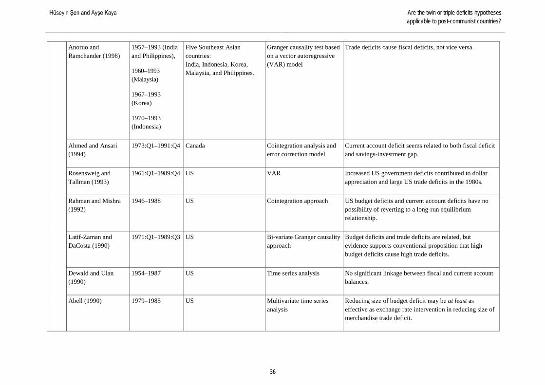
Hüseyin Şen and Ayşe Kaya Are the twin or triple deficits hypotheses applicable to post-communist countries?
36
Anoruo and Ramchander (1998)
1957–1993 (India and Philippines),
1960–1993 (Malaysia)
1967–1993 (Korea)
1970–1993 (Indonesia)
Five Southeast Asian countries: India, Indonesia, Korea, Malaysia, and Philippines.
Granger causality test based on a vector autoregressive (VAR) model
Trade deficits cause fiscal deficits, not vice versa.
Ahmed and Ansari (1994)
1973:Q1–1991:Q4 Canada Cointegration analysis and error correction model
Current account deficit seems related to both fiscal deficit and savings-investment gap.
Rosensweig and Tallman (1993)
1961:Q1–1989:Q4 US VAR Increased US government deficits contributed to dollar appreciation and large US trade deficits in the 1980s.
Rahman and Mishra (1992)
1946–1988 US Cointegration approach US budget deficits and current account deficits have no possibility of reverting to a long-run equilibrium relationship.
Latif-Zaman and DaCosta (1990)
1971:Q1–1989:Q3 US Bi-variate Granger causality approach
Budget deficits and trade deficits are related, but evidence supports conventional proposition that high budget deficits cause high trade deficits.
Dewald and Ulan (1990)
1954–1987 US Time series analysis No significant linkage between fiscal and current account balances.
Abell (1990) 1979–1985 US Multivariate time series analysis
Reducing size of budget deficit may be at least as effective as exchange rate intervention in reducing size of merchandise trade deficit.
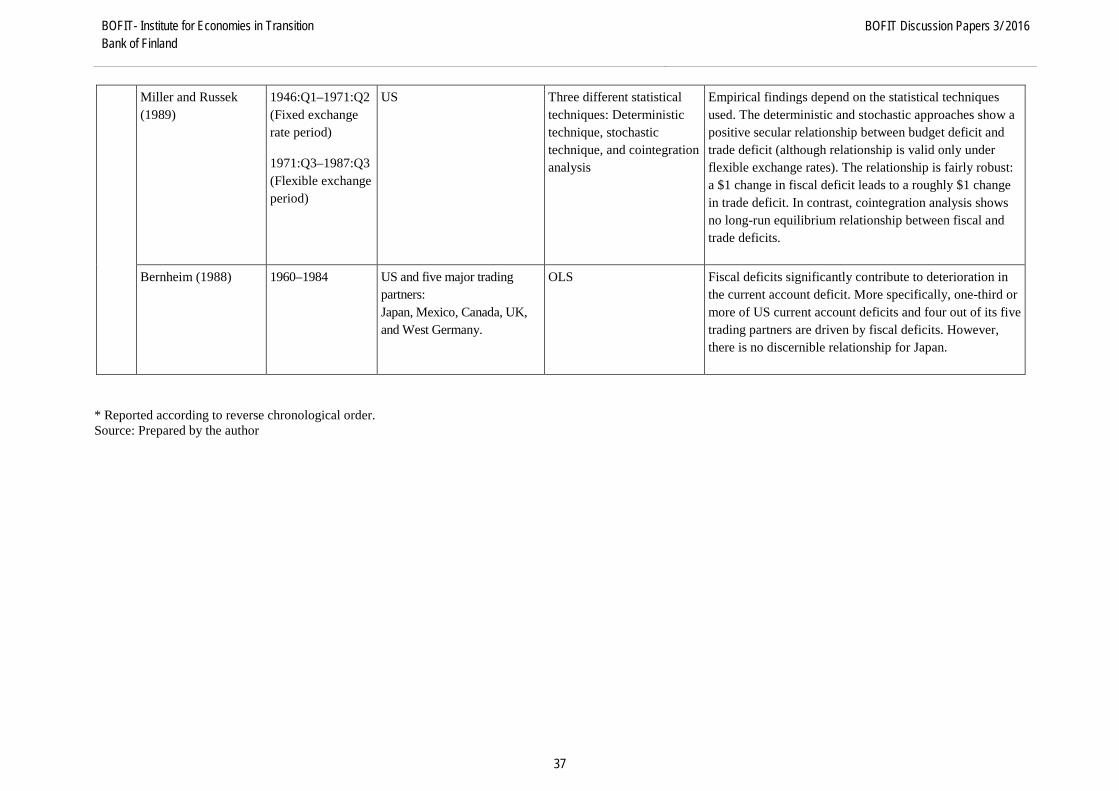
BOFIT- Institute for Economies in Transition Bank of Finland
BOFIT Discussion Papers 3/ 2016
37
Miller and Russek (1989)
1946:Q1–1971:Q2 (Fixed exchange rate period)
1971:Q3–1987:Q3 (Flexible exchange period)
US Three different statistical techniques: Deterministic technique, stochastic technique, and cointegration analysis
Empirical findings depend on the statistical techniques used. The deterministic and stochastic approaches show a positive secular relationship between budget deficit and trade deficit (although relationship is valid only under flexible exchange rates). The relationship is fairly robust: a $1 change in fiscal deficit leads to a roughly $1 change in trade deficit. In contrast, cointegration analysis shows no long-run equilibrium relationship between fiscal and trade deficits.
Bernheim (1988) 1960–1984 US and five major trading partners: Japan, Mexico, Canada, UK, and West Germany.
OLS Fiscal deficits significantly contribute to deterioration in the current account deficit. More specifically, one-third or more of US current account deficits and four out of its five trading partners are driven by fiscal deficits. However, there is no discernible relationship for Japan.
* Reported according to reverse chronological order. Source: Prepared by the author

Hüseyin Şen and Ayşe Kaya Are the twin or triple deficits hypotheses applicable to post-communist countries?
38
Appendix B Cross-sectional dependence and slope homogeneity tests14 Three tests are available to investigate the existence of cross-sectional dependence: the La-grange multiplier test statistic of Breusch and Pagan (1980) for cross-sectional dependence, and the cross-sectional dependence test statistics of Pesaran (2004), which are based either on Lagrange multiplier or pair-wise correlation coefficients.
The Lagrange Multiplier (LM) test developed by Breusch and Pagan (1980) re-quires estimation of the following panel data model: Yit = αI + βiXit + µit (1)
for I = 1,2, 3, …, N; t = 1,2, 3, …, T ,
where I is the cross section dimension; t is the time dimension; Xit is kx1 vector of explana-tory variables, and αI and βI are the individual intercepts and slope coefficients allowed to differ across states.
In the LM test, the null hypothesis of no cross-sectional dependence H0 : Cov (μit,μjt) = 0 for all t and I ≠ j is tested against the alternative hypothesis of cross-sectional dependence H1 : Cov (μit,μjt) ≠ 0 for at least one pair of i≠ j.
For testing the null hypothesis, the LM test statistic for cross-sectional dependence of Breusch and Pagan (CDBP) is given as:
CDBP = T1
1
N
i
−
=∑
1
N
j i= +∑ 𝜌𝜌�𝑖𝑖𝑎𝑎2 , (2)
where ρ�ij2 is the estimated correlation coefficient among the residuals obtained from indi-
vidual OLS estimation of Equation (1). Under the null hypothesis, the LM statistic has an asymptotic chi-square distribution with N (N-1)/2 degrees of freedom.
Pesaran (2004) indicates, however, that the CDBP test has a drawback when N is large, implying that it is not applicable when N→∞. To overcome this problem, the following LM statistic for cross-sectional dependence (CDLM) was developed by Pesaran (2004). The CDLM statistic is given as:
CDLM = � 1𝑁𝑁(𝑁𝑁−1)
1
1
N
i
−
=∑
1
N
j i= +∑ (𝑇𝑇𝜌𝜌�𝑖𝑖𝑎𝑎2 -1) (3)
Under the null hypothesis of no cross-sectional dependence with T→∞ and then N→∞, CDLM asymptotically follows a normal distribution.
Unfortunately, the CDLM test is likely to indicate size substantial distortions when N is large relative to T. Pesaran (2004) therefore proposes an alternative test for cross-sectional
14 These definitional equations heavily borrow from Şen et al. (2015).

BOFIT- Institute for Economies in Transition Bank of Finland
BOFIT Discussion Papers 3/ 2016
39
dependence (CD) that can be used where N is large and T is small. The CD statistic is calcu-lated as follows:
CD = � 2𝑇𝑇𝑁𝑁(𝑁𝑁−1)
1
1
N
i
−
=∑
1
N
j i= +∑ 𝜌𝜌�𝑖𝑖𝑎𝑎 (4)
Pesaran (2004) states that under the null hypothesis of no cross-sectional dependence with T → ∞ and N → ∞ in any order, the CD test is asymptotically normally distributed. Pesaran et al. (2008) qualify this by noting that when the population average pair-wise correlation is zero, the CD test has less power. Therefore, they propose a bias-adjusted LM test that uses the exact mean and variance of the LM statistic. The bias-adjusted LM statistic is calculated as follows:
CDadj = � 2𝑇𝑇𝑁𝑁(𝑁𝑁−1)
1
1
N
i
−
=∑
1
N
j i= +∑ 𝜌𝜌�𝑖𝑖𝑎𝑎
(𝑇𝑇−𝑘𝑘)𝜌𝜌�𝑖𝑖𝑖𝑖2 −𝑢𝑢𝑇𝑇𝑖𝑖𝑖𝑖
�𝑣𝑣𝑇𝑇𝑖𝑖𝑖𝑖2
, (5)
where uTij and vTij2 are the exact mean and variance of (T-k) ρ�ij2 , which are provided by
Pesaran et al. (2008). Under the null hypothesis of no cross-sectional dependence with T → ∞ first followed by N → ∞, the results of the CDadj test follow an asymptotic standard normal distribution.
The standard F-test is the most widely used way to test the null hypothesis of slope homogeneity H0 : βI = β for all I against the hypothesis of heterogeneity H1 : βI ≠ βj for a non-zero fraction of pair-wise slopes for i≠j. This requires that the explanatory variables are strictly exogenous and the error variances are homoscedastic. To relax the assumption of homoscedasticity in the F-test, Swamy (1970) developed a slope homogeneity test that examines the dispersion of individual slope estimates from a suitable pooled estimator.
Pesaran and Yamagata (2008) state that both the F-test and Swamy’s test require panel data models where N is relatively small compared to T. Therefore, they propose a standardized version of Swamy’s test (hereafter, ∆� test) for testing slope homogeneity in large panels. The ∆ test is valid when (N, T) → ∞ without any restrictions on the relative expansion rates of N and T when the error terms are normally distributed. Swamy’s statistic can then be modified as:
�̃�𝑆= 1
N
i=∑ ��̂�𝛽𝑖𝑖 − �̂�𝛽𝑊𝑊𝑊𝑊𝑊𝑊�
′ 𝑋𝑋𝑖𝑖
′𝑀𝑀𝜏𝜏𝑋𝑋𝑖𝑖𝜎𝜎�𝑖𝑖2 ��̂�𝛽𝑖𝑖 − �̂�𝛽𝑊𝑊𝑊𝑊𝑊𝑊� , (6)
where β�I is the pooled OLS estimator; β�WFE is the weighted fixed effect pooled estimator of the Equation (1); Mτ is an identity matrix of order T and σ�i
2 is the estimator of σi2.

Hüseyin Şen and Ayşe Kaya Are the twin or triple deficits hypotheses applicable to post-communist countries?
40
Pesaran and Yamagata (2008) further develop the following standardized disper-sion statistic: ∆� = √𝑁𝑁 �𝑁𝑁
−1�̃�𝑆−𝑘𝑘√2𝑘𝑘
� (7)
Under the null hypothesis with the condition of (N, T) → ∞ and so long as √N/T → ∞, and when the error terms are normally distributed, the ∆� test has an asymptotic standard normal distribution.
The small sample properties of the ∆� test can be improved when there are normally distributed errors by using the following mean and variance bias adjusted version: ∆�𝑎𝑎𝑎𝑎𝑎𝑎 = √𝑁𝑁 �𝑁𝑁
−1�̃�𝑆−𝑊𝑊(𝑍𝑍�𝑖𝑖𝑖𝑖)�𝑣𝑣𝑎𝑎𝑣𝑣(𝑍𝑍�𝑖𝑖𝑖𝑖)
� , (8)
where the mean E�Z�it� = k, and var�Z�it� = 2k(T-k-1)/(T+1).

BOFIT- Institute for Economies in Transition Bank of Finland
BOFIT Discussion Papers 3/ 2016
41
Appendix C Other results from bootstrap panel Granger causality analysis Table 1 reports the results of panel Granger causality between budget balance and private savings-investment balance.
Table 1 Panel Granger causality between budget balance (BB) and private savings-investment balance (SIB)
Country Estimated coefficient Wald Test
Bootstrap critical values Granger causality
Yes/No 10% 5% 1%
𝐇𝐇𝟎𝟎 : Budget deficits do not cause private savings-investment deficits
Russia –0.24031 4.15272 6.48159 9.26189 19.68549 No
Poland –0.80707 17.96319*** 6.17857 8.89016 17.64496 Yes
Ukraine 0.40719 2.12450 6.51380 10.25422 23.42109 No
Romania –0.92178 11.22914*** 8.89024 12.52762 20.61716 Yes
Czech Republic
–0.042763 0.16017 6.48803 9.43279 18.42607 No
Hungary 0.19414 2.21743 6.67243 9.46650 16.73213 No
𝐇𝐇𝟎𝟎 : Private savings-investment deficits do not cause budget deficits
Russia 0.79907 13.062135*** 6.26030 9.34477 19.20222 Yes
Poland 0.20153 3.35927 7.18930 10.81216 20.25727 No
Ukraine 0.23854 6.64324*** 5.57397 8.87024 16.31503 Yes
Romania 0.19820 6.41192 7.13433 10.90076 18.40454 No
Czech Republic
–0.061918 0.19565 8.18093 12.10320 24.55806 No
Hungary 0.77034 8.88738*** 5.56864 8.39067 14.68569 Yes
Notes: The data cover the whole sample period from 1994 to 2012. (***) indicates statistical significance at 10%. Source: Authors’ calculations Notably, there is a significant and negative Granger causality running from budget deficits to the private savings-investment deficits of Poland and Romania. Moreover, only three (Rus-sia, Ukraine, and Hungary) of our six countries exhibit significant and positive Granger cau-sality running from private savings-investment deficits to budget deficits. With the exception of the Czech Republic, the null hypothesis of no Granger causality from budget deficits to pri-vate savings-investment deficits or vice versa cannot be rejected.
Table 2 indicates significant and positive Granger causality running from private savings-investment deficits to trade deficits for Poland and Romania, but not the other four

Hüseyin Şen and Ayşe Kaya Are the twin or triple deficits hypotheses applicable to post-communist countries?
42
countries. On the other hand, our findings suggest the causal direction from trade deficits to private savings-investment deficits is valid for Russia, Ukraine, the Czech Republic, and Hungary, implying that the null hypothesis stands for these countries (i.e. there is no Granger causality in this direction). For Poland and Romania, however, there is significant, but negative, Granger causality running from trade deficits to private savings-investment deficits. Table 2 Panel Granger causality between private savings-investment balance (SIB) and trade balance (NXB)
Country Estimated coefficient Wald Test
Bootstrap critical values Granger causality
Yes/No 10% 5% 1%
𝐇𝐇𝟎𝟎 : Private savings-investment deficits do not cause trade deficits
Russia 0.022719 0.54678 6.73325 10.92829 20.78984 No
Poland 0.51413 8.65959*** 6.41573 8.45763 17.97478 Yes
Ukraine –0.23934 0.56873 6.37846 9.64867 15.51802 No
Romania 0.92680 21.10031*** 7.90944 11.82749 23.57803 Yes
Czech Republic
0.19803 0.55238 6.28098 10.14065 20.84300 No
Hungary –0.16903 0.91966 5.86125 8.56126 19.48040 No
𝐇𝐇𝟎𝟎 : Trade deficits do not cause private savings-investment deficits
Russia –0.34668 3.76326 6.70739 9.25943 20.20941 No
Poland –0.94011 22.18209*** 6.75525 10.10809 17.50172 Yes
Ukraine 0.43689 1.64086 7.59905 10.83030 21.06846 No
Romania –0.74606 11.84858*** 7.34579 11.34655 21.12873 Yes
Czech Republic
–0.12811 0.97950 6.41807 9.87203 20.66651 No
Hungary 0.22865 2.14292 6.04718 9.81700 19.71584 No
Notes: The data covers the whole sample period from 1994 to 2012. (***) indicates statistical significance at 10%. Source: Authors’ calculations

BOFIT Discussion Papers A series devoted to academic studies by BOFIT economists and guest researchers. The focus is on works relevant for economic policy and economic developments in transition / emerging economies.
BOFIT Discussion Papers http://www.bof.fi/bofit_en • email: [email protected]
ISSN 1456-4564 (print) // ISSN 1456-5889 (online)
2015 No 1 Qing He, Liping Lu and Steven Ongena: Who gains from credit granted between firms? Evidence from inter-corporate loan announcements Made in China No 2 Ke Pang and Pierre L. Siklos: Macroeconomic consequences of the real-financial nexus: Imbalances and spillovers between China and the U.S. No 3 V.V. Mironov, A.V. Petronevich: Discovering the signs of Dutch disease in Russia No 4 Joshua Aizenman: The internationalization of the RMB, capital market openness, and financial reforms in China No 5 Yu-Fu Chen, Michael Funke and Kunyu Tao: Financial market reform – A new driver for China’s economic growth? No 6 Jarko Fidrmuc and Iikka Korhonen: Meta-analysis of Chinese business cycle correlation No 7 Jarko Fidrmuc, Zuzana Fungáčová and Laurent Weill: Does bank liquidity creation contribute to economic growth? Evidence from Russia No 8 Elena Deryugina, Olga Kovalenko, Irina Pantina and Alexey Ponomarenko: Disentangling loan demand and supply shocks in Russia No 9 Michael Funke, Petar Mihaylovski and Haibin Zhu: Monetary policy transmission in China: A DSGE model with parallel shadow banking and interest rate control No 10 Riikka Nuutilainen: Contemporary monetary policy in China: A move towards price-based policy? No 11 Iftekhar Hasan, Nada Kobeissi, Haizhi Wang and Mingming Zhou: Banking structure, marketization and small business development: Regional evidence from China No 12 Linlin Niu, Xiu Xua and Ying Chen: An adaptive approach to forecasting three key macroeconomic variables for transitional China No 13 Heiner Mikosch and Stefan Neuwirth: Real-time forecasting with a MIDAS VAR No 14 Alexander Libman and Björn Vollan: Anti-Western conspiracy thinking and expectations of collusion: Evidence from Russia and China No 15 Mikhail Stolbov: Causality between credit depth and economic growth: Evidence from 24 OECD countries No 16 Kefei You: What drives China’s outward FDI? A regional analysis No 17 José R. Sánchez-Fung: Estimating the impact of monetary policy on inequality in China No 18 Christian Hattendorff: Economic concentration and finance: Evidence from Russian regions No 19 Alexey Porshakov, Elena Deryugina, Alexey Ponomarenko and Andrey Sinyakov: Nowcasting and short-term forecasting of Russian GDP with a dynamic factor model No 20 Qing He, Iikka Korhonen, Junjie Guo and Fangge Liu: The geographic distribution of international currencies and RMB internationalization No 21 Haining Wang, Zhiming Cheng and Russell Smyth: Does consuming more make you happier? Evidence from Chinese panel data No 22 Mikhail Mamonov and Andrei Vernikov: Bank ownership and cost efficiency in Russia, revisited No 23 Rui Mao and Yang Yao: Fixed exchange rate regimes, real undervaluation and economic growth No 24 Elena Deryugina, Alexey Ponomarenko, Andrey Sinyakov and Constantine Sorokin: Evaluating underlying inflation measures for Russia No 25 Christian Dreger, Jarko Fidrmuc, Konstantin Kholodilin and Dirk Ulbricht: The Ruble between the hammer and the anvil: Oil prices and economic sanctions No 26 Zuzana Fungáčová, Riikka Nuutilainen and Laurent Weill: Reserve requirements and the bank lending channel in China No 27 Simo Leppänen, Laura Solanko and Riitta Kosonen: Could climate change affect government expenditures? Early evidence from the Russian regions No 28 Mariarosaria Comunale: Current account and REER misalignments in Central Eastern EU countries: an update using the macroeconomic balance approach No 29 John Fernald, Eric Hsu and Mark M. Spiegel: Is China fudging its figures? Evidence from trading partner data No 30 Jyri Kinnunen and Minna Martikainen: Expected returns and idiosyncratic risk: Industry-level evidence from Russia No 31 John P. Bonin and Dana Louie: Did foreign banks “cut and run” or stay committed to Emerging Europe during the crises? No 32 Anna Krupkina and Alexey Ponomarenko: Deposit dollarization in emerging markets: modelling the hysteresis effect No 33 Paul-Olivier Klein and Laurent Weill: Is it worth issuing bonds in China? Evidence from stock market reactions
2016 No 1 Guonan Ma and Wang Yao: Can the Chinese bond market facilitate a globalizing renminbi? No 2 Iikka Korhonen and Riikka Nuutilainen: A monetary policy rule for Russia, or is it rules? No 3 Hüseyin Şen and Ayşe Kaya: Are the twin or triple deficits hypotheses applicable to post-communist countries?