Are fluctuations in natural gas consumption per capita transitory? Evidence from time series and...

lable at ScienceDirect

Energy xxx (2014) 1e13

Contents lists avai

Energy

journal homepage: www.elsevier .com/locate/energy

Are fluctuations in natural gas consumption per capita transitory?Evidence from time series and panel unit root tests

Muhammad Shahbaz a, Naceur Khraief b, c, d, *, Mantu Kumar Mahalik e, Khair Uz Zaman f

a Department of Management Sciences, COMSATS Institute of Information Technology, Lahore, Pakistanb Faculty of Economic Science and Management of Sousse, University of Sousse, Tunisiac University of Nice Sophia Antipolis, Franced GREDEG (Research Group on Law Economics and Management), Francee Amritapuri Campus, Amrita Vishwa Vidyapeetham University, Indiaf COMSATS Institute of Information Technology, Vehari Campus, Vehari, Pakistan

a r t i c l e i n f o

Article history:Received 13 May 2014Received in revised form26 September 2014Accepted 29 September 2014Available online xxx

Keywords:Natural gasUnivariate unit root testsThe first and second generation panel dataunit root tests

* Corresponding author. University of Sousse, FacuManagement, Erriadh City 4023, Sousse, Tunisia. Tel.:73 301 888.

E-mail addresses: [email protected] (M. Sh(N. Khraief), [email protected] (M.K. Mahalik(K.U. Zaman).

http://dx.doi.org/10.1016/j.energy.2014.09.0800360-5442/© 2014 Elsevier Ltd. All rights reserved.

Please cite this article in press as: ShahbazMand panel unit root tests, Energy (2014), htt

a b s t r a c t

The stationary properties of natural gas consumption are essential for predicting the impacts of exog-enous shocks on energy demand, which can help modeling the energy-growth nexus. Then, this paperproposes to investigate the panel unit root proprieties of natural gas energy consumption of 48 countriesover the period of 1971e2010. We apply the Harvey et al. [69] linearity test in order to determine thetype of the unit root tests (the Kruse (2010) nonlinear unit root or LM (Lagrange Multiplier) linear unitroot tests). Our results show that the stationarity of natural gas consumption cannot be rejected for morethan 60% of countries.

In order to provide corroborating evidence, we employed not only the first and second generationpanel unit root tests, but also the recent LM panel unit root test developed by Im et al. [28]. This testallows for structural breaks both in intercept and slope. The empirical findings support evidence in favorof stationarity of natural gas consumption for all panels. These results announce that any shock to naturalgas consumption has a transitory impact for almost all countries implying that energy consumption willturn back to its time trend.

© 2014 Elsevier Ltd. All rights reserved.

1. Introduction

Given the expanding size of economic activities, urbanization,industrialization and the resultant demand for energy use, therehas been an increasing tendency in the ‘energy economics litera-ture’ to test the unit root properties of energy consumption series ataggregate and disaggregate levels for managing energyeenviron-ment and energyegrowth relationships. Supporting the wisdomof this trend, the vast majority of empirical literature on thetopic applied various approaches and yielded mixed results[1,5e7,13,21,25,32,34,43,47,49,52,58,59,72]. Moreover, theseempirical investigations behind energy consumption stationarityare largely motivated by several factors. First, if energy

lty of Economic Sciences andþ216 73 301 808; fax: þ216

ahbaz), [email protected]), [email protected]

, et al., Are fluctuations in natup://dx.doi.org/10.1016/j.energ

consumption is stationary at level then shocks to energy con-sumption will have temporary effects over time and such designedeconomic policies will have transitory impact. For instance, if en-ergy consumption is stationary, shocks to energy consumption willbe fleeting or temporary following major structural changes inenergy consumption, the demand for energy consumption willreturn to its original equilibrium within a short period of time. Inthis case, disruptions in energy consumption demand will haveonly a transitory impact on economic activity. In such an environ-ment, the policymakers should not design any adverse policymechanism breaking the sound relationship between energy con-sumption and economic growth. Second, if energy consumptioncontains a unit root then shocks to energy consumption will havepermanent or long-term effects. In such environment, shocks toenergy consumption will have permanent effects on the level ofenergy demand. Hence disruptions in energy consumption willhave a permanent effect on economic activity and therefore thedesigned policies will be more effective. In addition, the extent towhich the energy sector is linked with others sectors of the econ-omy is also of larger significance as permanent shocks to energy

ral gas consumption per capita transitory? Evidence from time seriesy.2014.09.080

Delta:1_given name

Delta:1_surname

Delta:1_given name

Delta:1_surname

mailto:[email protected]




www.sciencedirect.com/science/journal/03605442

http://www.elsevier.com/locate/energy

http://dx.doi.org/10.1016/j.energy.2014.09.080



Table 1Survey of literature for stationary properties.

Authors Time period Unit root tests Conclusions

Lee and Chang [34] 1954e2003 Zevot and Andrew [63] structural break test I(1)Narayan and Smyth [72] 1954e2003 Zevot and Andrew [63] test I(1)Al-Iriani [1] 1979e2000 Univariate and IPS panel tests I(0)Soytas and Sari [61] 1971e2000 Carrion-i-Silvestre multiple test [12] I(0)Zachariadis and Pashouritdou [62] 1973e2008 LM structural break test I(0)Narayan and Smyth [46,72] 1971e2003 Panel seemingly unrelated regressions ADF I(1)Chen and Lee [13] 1973e2008 Long memory test Miscellaneous resultsHsu et al. [25] 1971e2003 Panel unit root test Mixed resultsNarayan et al. [49] 1973e2007 Lee and Strazicich [36] two structural breaks test I(0)Mishra et al. [43] 1980e2005 LLC, IPS and Maddala and Wu panel tests and CIPS test Miscellaneous resultsNarayan et al. [48] 1973e2007 Lee and Strazicich [36] univariate unit root tests

with up to two structural breaksI(0)

Apergis et al. [4] 1980e2007 LM structural break test I(0)Apergis et al. [5] 1982e2007 LM structural break test I(0)Aslan [6] 1960e2008 LM structural break test Miscellaneous resultsAslan and Kum [7] 1970e2006 LM structural break test I(0)Ozturk and Aslan [52] 1970e2006 Lee and Strazicich [36] two structural break test I(0)Hasanov and Telatar [24] 1980e2006 Non-Linear Test by Kapitaneous et al. (2003) Miscellaneous resultsKum [31] 1971e2007 Lee and Strazicich [35,36]; one structural break test I(0)Golpe et al. [21] 1973:1e2010:3 Non-linear specification of an unobserved components model Evidence of persistenceKula et al. [30] 1960e2005 LM structural break test I(0)Apergis and Tsoumas [3] 1989e2009 Fractional integration with structural breaks Mixed resultsMaslyuk and Dharmaratna [40] 1966e2009 Zevot and Andrew [63] and Clemente et al. [16]

univariate unit root tests with structural breaksMixed evidence of stationarity

Narayan and Popp [47,73] 1980e2006 Pesaran [53] panel unit root test without structural break I(1)Congregado et al. [17] 1973e2010 Non-linear specification of an unobserved components model Evidence of persistenceShahbaz et al. [59] 1971e2010 Lee and Strazicich [35,36] univariate unit root tests


Shahbaz et al. [58] 1965e2010 LM unit root test with one break and two breaks crash model I(0)Lean and Smyth [32] 1978e2010 Lee and Strazicich [35,36] univariate unit root tests


Lean and Smyth [33] 1965e2011 LM panel unit root test [55] with no structural breaks andLM unit root test [35] with one and two structural breaks.

I(0)

Bolat et al. [11] 1960e2009 KwiatkowskiePhillipseSchmidteShin (KPSS) unit root test I(0)Bolat et al.[10] 1971e2010 LM test with two breaks I(0)Barros et al. [8] 1973e2010 LM test with two breaks I(1)Meng et al. [41] 1960e2010 LM and RALS-LM unit root tests I(0)Barros et al. [9] 1994e2011 LM test with two breaks Evidence of persistenceOzcan [51] 1980e2009 [28,35,36] I(0)

1 The use of a relatively large of countries has the advantage that it is possible touse both a panel and structural breaks [60].

M. Shahbaz et al. / Energy xxx (2014) 1e132

consumption may well be transmitted to other sectors of theeconomy as well as to macroeconomic aggregates.

However, the distinction between temporary and permanentshocks to energy consumption has several implications for policy-makers, financial investors and producers. For policymakers, theforecasting of energy demand is important because it plays a vitalrole in formulating energy policies. It is tempting to argue thatefficient and timely energy supply for economic growth can bepossible after knowing the reliable forecasts of energy consumptionin future. For instance, if energy consumption is stationary, then thepast behavior of energy consumption enables policymakers in theforecasting process. On other hand, if energy consumption is non-stationary, then the past behavior of this variable can't be used informulating the forecasts of future demand and one would need tolook at other variables explaining energy consumption to generateforecasts of energy demand into the future [5,6,43,58,60].Furthermore, the issue of whether energy consumption is station-ary has important implications for modeling purpose. If unidirec-tional causality runs from energy consumption to real output, itshows that reducing energy consumption could lead to a fall inincome; however, if causation runs in the opposite direction thisprovides strong justification for implementing energy consumptionpolicies because economic growth is not dependent on energyconsumption [43]. Second, the unit root properties of energy priceshave important practical implications for financial investors. Ifenergy prices are mean reverting, it reveals that the price level willreturn to its trend path over time and that enables investors to

Please cite this article in press as: ShahbazM, et al., Are fluctuations in natand panel unit root tests, Energy (2014), http://dx.doi.org/10.1016/j.energ

forecast future movements in energy prices based on its pastbehavior, but if energy prices follow a randomwalk process, shocksto energy prices will be permanent and also will be difficult toforecast. Finally, the understanding of temporary and permanentshocks to energy consumption is important for producers toknowing the behavior of energy prices as they use energy as one ofthe inputs in the process of production [43].

Table 1 provides summary of existing studies investigatingwhether fluctuations in energy consumption are permanent ortransitory. These studies have applied various approaches to testthe stationary properties of energy consumption and providedconflicting results. Recently, Apergis et al. [4] investigated the sta-tionary process of natural gas consumption in 50 US states usingseveral panel unit root tests [27,38,39,22]. It is further important tonote that the findings of single country can't be generalized to othereconomies of the world due to the presence of structural breaksand the application of differential methodologies. Keeping thislimitation in mind, to date, there has been no empirical attempt ofexamining the stationary properties of natural gas consumptionacross numerous countries.1 We address this gap in the literatureand make an empirical attempt in investigating the unit rootproperties of natural gas consumption by applying the recentLagrange Multiplier (LM) panel unit root test developed by Im et al.

ural gas consumption per capita transitory? Evidence from time seriesy.2014.09.080

2 Availability of data has restricted our analysis to 48 countries.

M. Shahbaz et al. / Energy xxx (2014) 1e13 3

[28] with testing structural breaks in both the intercept and slope.The empirical findings of this study should enable the policymakersin designing the appropriate policy for macroeconomic stabiliza-tion as it is commonly believed that the policymakers are mainlyconcerned about the consistent and robustness of the results acrosseconomies.

Natural gas as part of non-renewable energy or fossil fuels isessential the way we live. Similarly, its production is also vital theway we produce and demand in the economy. Hence, natural gasproduction grew by 1.9%. The US (4.7%) once again recorded thelargest volumetric increase and remained the world's largest pro-ducer. Norway (12.6%), Qatar (7.8%), and Saudi Arabia (11.1%) alsosaw significant production increases, while Russia (�2.7%) had theworlds' largest decline in volumetric terms (The BP Statistical Re-view of World Energy, 2013) [77]. Given the rising production ofnatural gas across the noted sample countries in the world, it ap-pears to be an important input in the production of macroeconomicactivities. Rather, the sustainable natural gas production, securityand quality are also important in the country's development,prosperity and welfare. In this sense, it is necessary to look at thesignificance of natural gas production in achieving sustainableeconomic growth. Thus, the possibility of sustainable economicgrowth can be achieved if both the growth and natural gas pro-duction are cointegrated and moving together at the constant ratein the long run. In this line, the understanding of time seriesproperties of natural gas production is also found to be importantbecause of the effect of disruptions in natural gas production oneconomic activity. For instance, if natural gas production contains aunit root, gas shocks will have permanent effects on the level ofnatural gas supplied. Hence disruptions in natural gas productionwill have a permanent effect on economic activity. However ifnatural gas production is stationary, shocks to gas production willbe temporary following major structural changes in natural gasproduction, the supply of gas will return to its original equilibriumwith the passage of time in the short run. In this case, disruptions innatural gas production will have only a transitory impact on eco-nomic activity. From this time series perspective, we believe theimportance of natural gas production on economic activity as po-tential input and further the understanding of sustainable eco-nomic growth depending upon the nature of shocks to natural gasproduction. If shocks to natural gas production permanent, then thesustainable economic growth will be hampered because the speedat which economic growth is expected to increase, the intensity andadequacy of natural gas production are far behind mainly due tostructural shocks to gas supply. Moreover, this indicates that acountry's welfare and prosperity would necessarily be affected dueto the disproportionate relationship between natural gas produc-tion and economic growth. In this context, it can be suggested thatthe energy policy designed for country's development needs toensure quality, security and sustainable natural gas production forsustaining economic growth in the long run.

Non-renewable energy is comprised of coal, crude oil and nat-ural gas. Natural gas is not only an important foundation fuelamong fossil fuels but also helping the process of heating andelectricity generation. For instance, natural gas is the cleanest-burning fossil fuel, with 30% less carbon than oil and as much as60% less carbon than coal for Canada. Burning natural gas in place ofother fuels can reduce emissions and contribute to cleaner airquality. As noted by BP Energy Outlook (2012) [66], natural gas isexpected to be the fastest growing of the fossil fuels-with demandrising at an average of 1.9% a year. Non-OECD countries are ex-pected to generate 78% of demand growth. Liquefied Natural Gas(LNG) exports are expected to grow more than twice as fast as gasconsumption, at an average of 3.9% per year, and accounting for 29%of the growth in global gas supply to 2035. Although world natural

Please cite this article in press as: ShahbazM, et al., Are fluctuations in natuand panel unit root tests, Energy (2014), http://dx.doi.org/10.1016/j.energ

gas consumption grew by 2.2%, below the historical average of 2.7%,globally it accounted for 23.9% of primary energy consumptionbehind oil and coal. According to World Energy Outlook (WEO,2011) [76], global gas demand was estimated at 3427 billion cubicmeters (bcm) in 2012, up 2% from 2011 levels. Gas demand hasincreased by around 800 bcm over the last decade, or 2.8% per year.For comparison, 50 billion cubic meters (bcm) of natural gas isroughly equivalent to 7% of the US's consumption in 2012. TheUnited States, Russia, Iran and China are world's largest consumersof gas. The largest producers are Russia, the United States, Canadaand Iran. Since there has been continued significant worldwideenergy demand is expected to double between 2005 and 2050, thenatural gas will play a key role in the global energy mix and thusensure the required supply of fuel which is assumed to be sus-tainable in the future as it is by far the cleanest and cheaplyavailable fuel, with the lowest CO2 emissions. Such versatility ofnatural gas makes it an important foundation fuel among otherfossil fuels (coal and oil) and that could be another importantreason for researchers to study the stationarity of natural gasconsumption across economies.

The aim of this paper is to investigate the stationary propertiesof natural gas consumption per capita using data of 48 high, middleand low income countries for 1971e2010 period.2 To examine thestationary properties of natural gas consumption per capita, thefirst and second generation panel unit root tests along with therecent Lagrange Multiplier (LM) panel unit root test capturingstructural breaks in both the intercept and slope have beenemployed.

The contributions of this paper are twofold. First, after testingthe cross-section correlation between units, we provide evidence ofstationarity of natural gas consumption for more than 40 countriespanel by applying panel unit root tests which allow dependenceacross different units in the panel; the so called “second genera-tion” panel unit root tests. Such issue has been neglected by theprevious studies on energy consumption stationarity [4,5,13,25,46](Narayan et al., 2008; [65,73]). Then, in presence of cross sectiondependence, this requests to be accounted for by using the secondgeneration tests and gain the high power proprieties of these tests.The second contribution is that we consider a structural breakpanel unit root test approach. For robustness check, the panel unitroot test of Im et al. [28] is performed. Using the ILT [28] test withstructural breaks we find robust evidence supporting the statio-narity of natural gas consumption for all the panels (high incomegroup countries, middle income countries and low income coun-tries panel) which corroborate the findings of both the first andsecond generation panel data unit root tests, leading us to concludethe importance of accounting for inter-dependence and structuralbreaks when testing for unit root in natural gas consumption in allgroups of countries. Thus, our results suggest that policies toencourage natural gas use will have temporary positive shocks.

The remainder of the paper is organized as follows: Section 2describes methodology and data. Section 3 presents results andSection 4 concludes the paper.

2. Methodology

2.1. Univariate unit root tests

The first stepwe take into account the possibility of nonlinearityof energy consumption series by testing the null hypothesis of timeseries linearity against a nonlinear alternative. Therefore, we usethe Harvey et al. [69] test which has better size control and offers



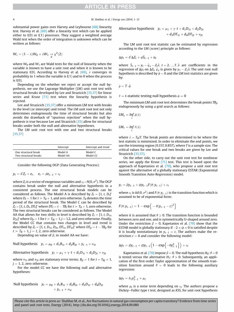
substantial power gains over Harvey and Leybourne [68] linearitytest. Harvey et al. [69] offer a linearity test which can be appliedeither to I(0) or I(1) processes. They suggest a weighted averageWald test when the order of integration is unknown which can bewritten as follows:

Wl ¼ ð1� lÞW0 þ lW1 /dc2ð2Þ

where W0 and W1 are Wald tests for the null of linearity when thevariable is known to have a unit root and when it is known to bestationary I(0). According to Harvey et al. [69], l converges inprobability to 1 when the variable is I(1) and to 0 when the processis I(0).

Depending on the whether we reject or accept the null hy-pothesis, we use the Lagrange Multiplier (LM) unit root test withstructural breaks developed by Lee and Strazicich [35,37] for linearseries and Kruse [71] test when the linearity hypothesis isrejected.

Lee and Strazicich [35,37] offer a minimum LM test with breaksin the level (or intercept) and trend. The LM unit root test not onlydetermines endogenously the time of structural breaks but alsoavoids the drawback of “spurious rejection” when the null hy-pothesis is true because Lee and Strazicich [35] allow for structuralbreaks under both the null and alternative hypotheses.

The LM unit root test with one and two structural breaks[35,37]

Intercept Intercept and trend

One structural break Model A Model CTwo structural breaks Model AA Model CC

Consider the following DGP (Data Generating Process):

yt ¼ d0Zt þ et ; et ¼ bet�1 þ 3t

where Zt is a vector of exogenous variables and 3t ~N(0, s2). The DGPcontains break under the null and alternative hypothesis in aconsistent process. The one structural break models can beconsidered as follows. The Model A is described by Zt ¼ [1, t, Dt]0

where Dt ¼ 1 for t_ TB þ 1, and zero otherwise. TB denotes the timeperiod of the structural break. The Model C can be described byZt ¼ [1, t, Dt, DTt]0 where DTt ¼ t � TBt for t_ TB þ 1, zero otherwise.The two structural breaks can be considered as follows. The ModelAA that allows for two shifts in level is described by Zt ¼ [1, t, D1t,D2t]0 whereDjt¼ 1 for t_ TBjþ 1, j¼ 1,2, and zero otherwise. Finally,the Model CC that contains two changes in level and trend isdescribed by Zt ¼ [1, t, D1t, D2t, DT1t, DT2t]0 where DTjt ¼ t � TBjt fort _ TB þ 1, j ¼ 1, 2, zero otherwise.

Depending on value of b, in model AA we have:

Null hypothesis yt ¼ m0 þ d1B1t þ d2B2t þ yt�1 þ v1t

Alternative hypothesis yt ¼ m1 þ g$t þ d1D1t þ d2D2t þ v2t

where v1t and v2t are stationary error terms; Bjt ¼ 1 for t ¼ TBj þ 1,j ¼ 1, 2, zero otherwise.

For the model CC we have the following null and alternativehypotheses:

Null hypothesis yt ¼ m0 þ d1B1t þ d2B2t þ d3D1t þ d4D2t

þ yt�1 þ v1t


Alternative hypothesis yt ¼ m1 þ g$t þ d1D1t þ d2D2t

þ d3DT1t þ d4DT2t þ v2t

The LM unit root test statistic can be estimated by regressionaccording to the LM (score) principle as follows:

Dyt ¼ d0DZt þ f~St�1 þ ut

where ~St�1 ¼ yt � ~jx � Zt~d; t ¼ 2; :::; T ;~d are coefficients in theregression of Dyt on DZt, ~jx is given by y1 � Z1~d. The unit root nullhypothesis is described by f¼ 0 and the LM test statistics are givenby:

~r ¼ T$~f

~t ¼ tstatistic testing null hypothesis f ¼ 0

The minimum LM unit root test determines the break points TBjtendogenously by using a grid search as follows:

LMr ¼ Infl

~rðlÞ

LMt ¼ Infl

~tðlÞ

where l ¼ TB/T. The break points are determined to be where thetest statistic is minimized. In order to eliminate the end points, weuse the trimming region (0.15T, 0.85T), where T is a sample size. Thecritical values for one break and two breaks are given by Lee andStrazicich [35,37].

On the other side, to carry out the unit root test for nonlinearseries, we apply the Kruse [71] test. This test is based upon theapproach of Kapetanios et al. [70], who propose a unit root testagainst the alternative of a globally stationary ESTAR (ExponentialSmooth Transition Auto-Regression) model.

yt ¼ byt�1 þ∅yt�1Fðq; yt�1Þ þ 3t

where 3t is iidð0; s2Þ and Fðq; yt�1Þ is the transition functionwhich isassumed to be of exponential form:

Fðq; yt�1Þ ¼ 1� expn� qðyt�1 � cÞ2

owhere it is assumed that q � 0. The transition function is boundedbetween zero and one, and is symmetrically U-shaped around zero.Under the restriction b ¼ 0, Kapetanios et al. [70] show that theESTAR model is globally stationary if �2 < ∅ < 0 is satisfied despiteit is locally nonstationary in yt�1 ¼ c. The authors make the re-striction c ¼ 0 and consider the following model:

Dyt ¼ byt�1 þ∅yt�1

�1� exp

n�qy2t�1

o�þ 3t

Kapetanios et al. [70] impose b¼ 0. The null hypothesis H0: q¼ 0is tested versus the alternative H1: q > 0. Subsequently, an appli-cation of the first-order Taylor approximation of the smooth tran-sition function around q ¼ 0 leads to the following auxiliaryregression:

Dyt ¼ d1y3t�1 þ mt

where mt is a noise term depending on 3t. The authors propose aDickeyeFuller type t test, designed as KSS, for unit root hypothesis


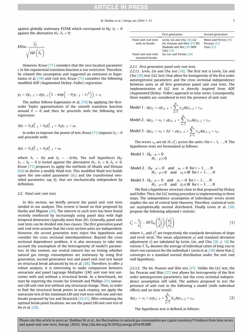
First generation Second generation

Panel unit root testswith no breaks

Levin, Lin and Chu [38] LLC Moon and Perron [44]Im, Pesaran and Shin [27] IPS Pesaran [53]Maddala and Wu [39] MW Choi [15]Choi [14]

Panel unit root withstructural breaks

Im, Lee and Tieslau [28]


against globally stationary ESTAR which correspond to H0: d1 ¼ 0against the alternative H1: d1 < 0:

KSS≡cd1ffiffiffiffiffiffiffiffiffiffiffiffiffiffiffiffiffiffiffiffidvar�cd1�

s

However, Kruse [71] considers that the zero location parameterc in the exponential transition function is too restrictive. Therefore,he relaxed this assumption and suggested an extension to Kape-tanios et al. [70] unit root test. Kruse [71] considers the followingmodified ADF (Augmented DickeyeFuller) regression:

yt ¼ byt�1 þ∅yt�1

�1� exp

n� qðyt�1 � cÞ2

o�þ 3t

The author follows Kapetanios et al. [70] by applying the first-order Taylor approximation of the smooth transition functionaround q ¼ 0 and then he proceeds with the following testregression:

Dyt ¼ d1y3t�1 þ d2y

2t�1 þ d3yt�1 þ mt

In order to improve the power of test, Kruse [71] imposes d3 ¼ 0and proceeds with:

Dyt ¼ d1y3t�1 þ d2y

2t�1 þ mt

where d1 ¼ q∅ and d2 ¼ �2cq∅. The null hypothesis H0:d1 ¼ d2 ¼ 0 is tested against the alternative H1: d1 < 0, d2 s 0.Kruse [71] proposes to apply the methods of Abadir and Distaso[64] to derive a modify Wald test. This modified Wald test buildsupon the one-sided parameter (d1) and the transformed two-sided parameter, say d2

⊥, that are stochastically independent bydefinition.

2.2. Panel unit root tests

In this section, we briefly present the panel unit root testsneeded in our analysis. This review is based on that proposed byHurlin and Mignon [26]. The interest in such tests has been foundrecently reinforced by increasingly using panel data with hightemporal dimension (typically more than 20). Generally, panel unitroot tests can be divided into two classes. The first generation panelunit root tests assume that the cross section units are independent.However, the second generation tests reject this hypothesis andconsider the cross sectional interdependence. Beyond the crosssectional dependence problem, it is also necessary to take intoaccount the assumption of the heterogeneity of model's parame-ters. In this context, our central interest lies on testing whethernatural gas energy consumptions are stationary by using firstgeneration, second generation test and panel unit root test basedon structural break advanced by Im et al. [28]. Therefore, to offer arobust analysis, it is interesting to make comparison betweenunivariate and panel Lagrange Multiplier (LM) unit root test out-comes with and without a structural break. As a benchmark, westart by reporting the results for Schmidt and Phillips [55] univar-iate LM unit root test without any structural change. Then, in orderto find the structural break points in each country, we apply theunivariate test of the minimum LM unit root tests with one and twobreaks proposed by Lee and Strazicich [35,37]. After estimating theoptimal break-point locations, we use the panel LM unit root test ofIm et al. [28].


2.2.1. First generation panel unit root tests2.2.1.1. Levin, Lin and Chu test [38]. The first test is Levin, Lin andChu [38] test (LLC test) that allow for homogeneity of the first orderautoregressive parameters and the cross sectional independencebetween units as all first generation panel unit root tests. Theimplementation of LLC test is directly inspired from ADF(Augmented DickeyeFuller) approach in time series. Consequently,three models are considered to test the presence of unit root:

Model 1 : Dyi;t ¼ ryi;t�1 þXpi

j¼1

gi;jDyi;t�j þ 3i;t

Model 2 : Dyi;t ¼ ai þ ryi;t�1 þXpi

s¼1

gi;sDyi;t�j þ 3i;t

Model 3 : Dyi;t ¼ ai þ bit þ ryi;t�1 þXpi

j¼1

gi;jDyi;t�j þ 3i;t

The errors 3i,t are iid ð0; s23i Þ across the units i for i ¼ 1, …, N. Thehypotheses tests are formulated as follows:

Model 1 : H0 : r ¼ 0H1 : r<0

Model 2 : H0 : r ¼ 0 and ai ¼ 0 for i ¼ 1;…;NH1 : r<0 and ai2IR for i ¼ 1;…;N

Model 3 : H0 : r ¼ 0 and bi ¼ 0 for i ¼ 1;…;NH1 : r<0 and bi2IR for i ¼ 1;…;N

We find a hypotheses structure close to that proposed by Dickeyand Fuller. Then, the LLC testing procedure is implementing in threesteps. The independence assumption of individuals' errors termsimplies the use of central limit theorem. Therefore, statistical testsare asymptotically normal distributed. Finally Levin et al. [38]propose the following adjusted t statistic:

t*r ¼ trs*T

� NTbSN bsbrbs2

~3

! m*T

s*T

!(1)

where bsbr and bs2~3are respectively the standards deviations of slope

and error term. The mean adjustment mT* and standard deviation

adjustment sT* are tabulated by Levin, Lin, and Chu [38, p. 14] forvarious T. bSN denotes the average of individual ratios of long-run toshort-run variances for the individual i. Levin et al. [38] show that tr*

converges to a standard normal distribution under the unit rootnull hypothesis.

2.2.1.2. The Im, Pesaran and Shin test [27]. Unlike the LLC test, theIm, Pesaran and Shin [27] test allows for heterogeneity of the firstorder autoregressive parameters, but the cross sectional indepen-dence assumption still valid. The authors proposed to test thepresence of unit root in the following a model (with individualeffects and no time trend):

Dyi;t ¼ ai þ riyi;t�1 þXpi

j¼1

bi;jDyi;t�j þ 3i;t (2)

The hypothesis test is defined as follows:



H0 : ri ¼ 0 for i ¼ 1;…;N

H1 :

�ri <0 for i ¼ 1;…;N1ri ¼ 0 for i ¼ N1 þ 1;N1 þ 2;…;N

Under the alternative hypothesis, the individual series yi,t couldbe divided into subgroups. More specifically, there areN1 stationaryseries and N � N1 series which admit unit roots. To perform thistest, the authors propose two statistics. The first one is the stan-dardized statistics Ztbar(p; b), centered and reduced respectively bythe mean and standard deviation of the limiting distribution ofindividual Augmented DickeyeFuller statistics:

Ztbarðp; bÞ ¼ffiffiffiffiN

p½tbarNT � EðtiT Þ�ffiffiffiffiffiffiffiffiffiffiffiffiffi

VðtiT Þp (3)

with tbarNT ¼ 1=NXNi¼1

tiT

where tiT designates the t-statistic associatedwith the unit root nullhypothesis (ri ¼ 0). In a model with individual effects and no timetrend, the limiting distribution moments are defined byE(tiT) ¼ �1.533 and V(tiT) ¼ 0.706 [45]. The statistic Ztbar(p;b)sequentially converge to the standard normal distribution whenT/∞ followed byN/∞. However, ifN is small then IPS test showsize distortions.3 It is for that reason that Im et al. [27] have pro-posed (under the null hypothesis ri¼ 0) an alternative standardizedstatistic Wtbar(p; b) that have better small sample performance:

Wtbarðp; bÞ ¼ffiffiffiffiN

p htbarNT � N�1PN

i¼1EðtiT ðri;0Þjri ¼ 0Þi

ffiffiffiffiffiffiffiffiffiffiffiffiffiffiffiffiffiffiffiffiffiffiffiffiffiffiffiffiffiffiffiffiffiffiffiffiffiffiffiffiffiffiffiffiffiffiffiffiffiffiffiffiffiffiffiffiffiffiffiN�1

PNi¼1VðtiT ðri;0Þjri ¼ 0Þ

q (4)

The authors simulated the values of E(tiT(ri,0)jri ¼ 0) andV(tiT(ri,0)jri ¼ 0) for different values of periods T and lag orders p.However, if N is relative large to T the IPS test shows size distortions(the null hypothesis will be rejected too often).

2.2.1.3. The Maddala and Wu [39] and Choi [14] tests.Maddala andWu [39] and Choi [14] suggested the use of Fisher [19]type test which is based on the idea of combining the p-values pifrom unit root test-statistics for each cross-sectional unit i. MaddalaandWu [39] affirm that when the test-statistics are continuous, thepi are independent uniform (0, 1) variables. Therefore, �2 ln(pi)follows the chi-squared distribution with two degrees of freedom.So, for a set of independent statistics, Maddala and Wu [39] haveproposed the following statistics:

PMW ¼ �2XNi¼1

lnðpiÞ (5)

has a c2 distribution with 2N degrees of freedom as T / ∞ and Nfixed. The statistic proposed by Choi [14] defined as:

ZMW ¼ffiffiffiffiN

p �N�1PMW � E½ � 2 lnðpiÞ�

ffiffiffiffiffiffiffiffiffiffiffiffiffiffiffiffiffiffiffiffiffiffiffiffiffiffiffiffiV ½ � 2 lnðpiÞ�

p (6)

Under the null hypothesis as Ti /∞ and N/∞, ZMW / N(0, 1).

2.2.2. Second generation panel unit root testsThree second generation tests will be now discussed. These tests

allow for cross sectional dependence to define a new statistic tests.

3 Similarly to LLC test.


More specifically, we present three tests [15,44,53] to test thepresence of unit root.

2.2.2.1. Moon and Perron (MP) [44] test. Moon and Perron [44] arebased on factor model to test the presence of a unit root in crosssectional dependent panel. The authors assume an AR(1) modeland the presence of common factors in the error term:

yi;t ¼ ð1� liÞmi þ liyi;t þ ui;t (7)

ui;t ¼ d0iFt þ ei;t

For i ¼ 1, …, N and t ¼ 1, …, T. Ft is a (k � 1) vector of commonsfactors, di is the coefficients vector corresponding to the commonfactors and ei,t is an idiosyncratic error term which is cross-sectionally uncorrelated and follows an infinite MA (MovingAverage) process. So, we have ei;t ¼

P∞j¼0gi;jL

j3i;t�j with 3i,t ~ iid(0,1). The common factors follow an infinite MA, Ft ¼

P∞j¼0∅jLjhi;t�j

with hi,t ~ iid(0, Ik) Moon and Perron [44] are testing the followingunit root null hypothesis H0: li ¼ 1 for i ¼ 1, …, N against theheterogenous alternative hypothesis H1: li < 1 for some i. After, tostudy the local power proprieties of this test, the authors examinethe following local alternative hypothesis:

li ¼ 1� qiffiffiffiffiN

pT

(8)

where qi is a random variable with mean mq. Then, the hypothesestest become H0

0: m0 ¼ 0 against the local alternative hypothesis H10:

m0 > 0. Moreover, the authors proposed for each ei,t the followingshort run and long run variances: s2ei ¼

P∞j¼0g

2i;j and

u2ei ¼ ðP∞

j¼0gi;jÞ2. The sum of positive autocovariance of idiosyn-cratic error term is defined as 4ei ¼

P∞l¼1P∞

j¼0gi;jgi;jþl. The non-zeroaverages of these parameters can be written as follows:

s2e ¼ 1N

XNi¼1

s2ei ; u2e ¼ 1

N

XNi¼1

u2ei and 42

e ¼ 1N

XNi¼1

42ei (9)

The testing method suggested by Moon and Perron [44] issummarized as follows. First, the authors proposed a pooled Or-dinary Least Squares (OLS) estimation of the first order autore-gressive coefficient. Next, they use this estimator to build up anestimate of the error terms bui;t ¼ yi;t � blyi;t�1 via the principalcomponent analysis and then attain an estimate of the (N � k)matrix D̂ ¼ ðbd1;…; bdNÞ. Finally, in order to remove the commonfactor effects from the original data (de-factoring the data), thematrix D̂ is used to construct the following projection matrix:QD̂ ¼ IN � D̂ðD̂0

D̂Þ�1D̂0. Then, the modified pooled estimator pro-

posed by Moon and Perron [44] is:

bl* ¼ trYt�1QD̂Y

0t�� NT4e

trYt�1QD̂Y

0t�1

� (10)

where tr($) is the trace operator and Yt ¼ (y1,t, …, yN,t). From thisconsistent estimator, Moon and Perron [44] suggested the use of thefollowing two t-statistics, denoted as ta

* and tb*, for testing the ho-

mogenous unit root hypothesis against heterogenous alternative:

t*a ¼ffiffiffiffiN

pT�bl* � 1

�ffiffiffiffiffiffiffi2b44

ebu4e

s /T ;N/∞

Nð0;1Þ (11)


Table 3Descriptive statistics.

Countries Mean Std. dev. Skewness Kurtosis JarqueeBera(prob. > c2)


t*b ¼ffiffiffiffiN

pT�bl* � 1

� ffiffiffiffiffiffiffiffiffiffiffiffiffiffiffiffiffiffiffiffiffiffiffiffiffiffiffiffiffiffiffi1

NT2trYt�1QD̂

rY 0t�1� bueb42

e

!/

T ;N/∞Nð0;1Þ

(12)
High income
countries406.2609 255.7349 0.0757 1.7608 0.000

Middle incomecountries

333.6083 196.5695 0.0333 1.8082 0.000

Low incomecountries

128.0857 75.8450 0.0548 1.7934 0.000

2.2.2.2. The Choi [15] test. For testing the presence of unit root, Choi[15] proposes to transform the observed series yi,t in order toeliminate the cross-sectional correlations and controlling fordeterministic trends. Consequently, Choi [15] discusses thefollowing error component model:

yit ¼ ai þ qt þ yi;t (13)

yi;t ¼Xpi

j¼1

di;jyi;t�1 þ 3i;t

where 3i,t is iidð0; s23i Þ. Firstly, to test the presence of unit root in theindividual component, it is necessary to orthogonalize the series yi,tthe cross-sectional dependence. Therefore, Choi [15] proposes toisolate yi,t by eliminating the individual and time effects ai and qt.The result is a new variable fzi;tgTt¼2. From this variable, it is thennecessary to perform a unit root test without constant and trendsince the entire deterministic components have been removed:

Dzi;t ¼ rizi;t�1 þXpi�1

j¼1

bi;jDzi;t�j þ ui;t (14)

Finally Choi [15] suggests combining the p-value pi of Dick-eyeFuller unit root t-statistics in each cross-sectional unit and us-ing the following three statistics:

Pm ¼ � 1ffiffiffiffiN

pXNi¼1

½lnðpiÞ þ 1�/T ;N/∞

Nð0;1Þ (15)

Z ¼ � 1ffiffiffiffiN

pXNi¼1

F�1ðpiÞ/T ;N/∞

Nð0;1Þ (16)

L* ¼ � 1ffiffiffiffiffiffiffiffiffiffiffiffiffiffiffip2N

�3

q XNi¼1

N ln�

pi1� pi

�/T ;N/∞

Nð0;1Þ (17)

where F is the standard cumulative normal distribution function.

Table 2Countries in the sample by income.

Country/income Number

High income countriesAustralia, Austria, Canada, Czech Republic, Finland,

France, Germany, Greece, Hungary, Italy, Japan,New Zealand, Norway, Poland, Portugal,Republic of Ireland, Slovakia, South Korea, Spain,Sweden, Switzerland, United States and UnitedKingdom

23

Middle income countriesAlgeria, Argentina, Brazil, Bulgaria, Chile, China,

Colombia, Ecuador, Iran, Malaysia, Mexico, Peru,Romania, South Africa, Taiwan, Thailand, Turkeyand Venezuela

18

Low income countriesBangladesh, Egypt, India, Indonesia, Pakistan,

Philippines and Vietnam7

Total countries 48


2.2.2.3. The Pesaran [53] test. Under the assumption of no serialcorrelation in the residuals, Pesaran [53] keeps the same IPS teststructure except that he considers an unobserved common factor ftwith an individual specific factor loading coefficient gi:

ui;t ¼ giqt þ 3i;t (18)

where 3i;t � iidð0; s2i Þ and E(3i,t4 ) < ∞. To test of the presence of unitroot, Pesaran [53] proposes to augment the DickeyeFuller orAugmented DickeyeFuller model by introducing a cross sectionaverage of lagged levels and first-differences of the individual seriesas follows:

Dyi;t ¼ ai þ riyi;t�1 þ ci

"ð1=NÞ

XNi¼1

yi;t�1

#

þ di

"ð1=NÞ

XNi¼1

Dyi;t

#þ 3i;t

(19)

The t-statistic of the OLS estimate of ri is denoted as ti(N, T)which is referred to CADF (Cross Sectionally Augmented Dick-eyeFuller) statistic for i. Based on the average of individual statis-tics, it is possible to build the following panel root t-statistic definedas Cross Sectional Augmented IPS:

CIPSðN; TÞ ¼ 1N

XNi¼1

tiðN; TÞ (20)

2.2.3. Panel unit root tests with structural break (third generationpanel unit root tests)

The first and second generation panel unit root tests may sufferfrom significant loss of power if the data contains structural breaks.In this case, it is complicated to distinguish between unit root andstationary processes with structural breaks. Today, the panel dataunit root tests which allow for structural breaks have receivedconsiderable attention among econometricians. In this section wediscuss the Lagrange Multiplier (LM)-based4 unit-root test devel-oped by Im et al. [28].

2.2.3.1. Im, Lee and Tieslau [28] structural break unit root test.In order to test the presence of unit root in the presence of struc-tural break, Im et al. [28] consider a data panel model with N cross-sectional units and T periods per unit and assume that structuralbreak happened at the time TB,i for unit i:

Yi;t ¼ g0iZi;t þ ui;t (21)

ui;t ¼ diui;t�1 þ 3i;t

4 The LM unit root test can be described by the following model: yt ¼ d0Zt þ utwith ut ¼ but�1 þ 3t.. Lee and Strazicich [35,37] develop versions of univariate LMunit-root test with one and two structural breaks (Models: A, AA, C and CC).


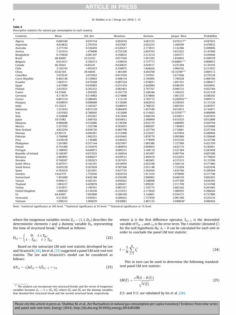
Table 4Descriptive statistics for natural gas consumption in each country.

Countries Mean Std. dev. Skewness Kurtosis JarqueeBera Probability

Algeria 0.066340 0.035754 0.891810 3.681533 6.076317** 0.047923Argentina 4.834832 2.701010 0.037687 2.052253 1.506509 0.470832Australia 3.277194 0.336459 �0.545617 2.173815 3.122286 0.209896Austria 7.161914 1.479000 �0.755330 2.895703 3.821622 0.147960Bangladesh 0.176650 0.081347 0.358632 2.313214 1.643571 0.439646Brazil 48.45605 23.22252 0.017594 1.951393 1.834693 0.399578Bulgaria 0.633411 0.184313 1.038918 5.737773 19.68801*** 0.000053Canada 66.25641 14.85241 �0.630635 2.024517 4.237284 0.120195Chile 3.192193 1.601653 0.358875 1.844426 3.084192 0.213932China 43.02184 39.44045 1.481449 4.456700 18.16789*** 0.000113Colombia 5.633535 2.672052 �0.012556 1.747021 2.617646 0.270138Czech Republic 0.462146 0.129603 0.498154 2.705095 1.799328 0.406706Ecuador 1.062511 0.679268 �0.007524 1.934831 1.891351 0.388417Egypt 2.415986 0.630483 �0.251419 2.442084 0.940195 0.624941Finland 2.832921 0.392332 0.065463 2.797767 0.096733 0.952784France 14.27649 1.956305 �0.191778 2.249344 1.184332 0.553128Germany 4.173679 0.514982 �0.274088 3.579866 1.061235 0.588242Greece 0.801314 0.288445 1.112118 3.783715 9.269056*** 0.009711Hungary 0.038055 0.008680 0.110286 4.602014 4.358503 0.113126India 15.19223 5.345567 0.640019 2.788525 2.805363 0.245937Indonesia 1.331653 0.872129 0.084459 1.457549 4.012815 0.134471Iran 1.619362 0.786045 1.612668 6.119422 33.55597*** 0.000000Italy 9.326898 1.023267 0.413944 3.946334 2.634911 0.267816Japan 18.51082 1.649742 0.034012 2.506069 0.414325 0.812888Malaysia 0.986688 0.552886 0.138396 2.032155 1.688896 0.429794Mexico 5.357592 1.352708 0.503055 2.806507 1.749493 0.416968New Zealand 4.822254 0.838726 �0.483798 2.167794 2.714681 0.257344Norway 23.99119 4.696381 �0.315498 2.235437 1.637854 0.440904Pakistan 3.796998 1.902252 �0.010445 1.878770 2.095990 0.350640Peru 2.639228 1.138488 0.249263 1.774999 2.915256 0.232788Philippines 1.241085 0.557144 0.027607 1.983386 1.727589 0.421559Poland 0.741480 0.163076 �0.468954 2.094663 2.832176 0.242661Portugal 2.188993 0.644072 0.609215 3.168110 2.521384 0.283458Republic of Ireland 0.168387 0.027635 �0.166934 2.301997 0.997794 0.607200Romania 2.985893 0.846657 �0.039512 2.445610 0.522655 0.770029Slovakia 0.740287 0.302623 0.267433 1.482401 4.315315 0.115596South Africa 0.287911 0.162181 0.618959 2.922348 2.564116 0.277466South Korea 0.695220 0.267828 0.507506 2.951148 1.721058 0.422938Spain 6.783419 1.623501 0.427735 2.392026 1.835766 0.399364Sweden 14.62379 1.752036 0.024724 1.911419 1.979090 0.371746Switzerland 7.491609 0.842188 �0.256209 2.960962 0.440159 0.802455Taiwan 0.999211 0.202101 0.050422 2.548098 0.357309 0.836395Thailand 1.065237 0.429078 0.209437 1.899287 2.311709 0.314788Turkey 5.353917 3.199761 0.087527 1.743775 2.681242 0.261683United Kingdom 1.004563 0.134330 �0.337815 2.173029 1.900595 0.386626Us 64.43097 7.093890 0.280109 3.136601 0.554172 0.757989Venezuela 9.212935 5.939431 0.206422 1.727839 2.981390 0.225216Vietnam 1.998252 1.984639 0.830882 2.487125 5.040838* 0.080426

Note: *statistical significance at 10% level. **Statistical significance at 5% level. ***Statistical significance at 1% level.


where the exogenous variables vector Zi,t ¼ (1, t, Di,t) describes thedeterministic elements t and a dummy variable Di,t representingthe time of structural break,5 defined as follows:

Di;t ¼�

0; t < TB;it � TB;i; t � TB;i

(22)

Based on the univariate LM unit root statistic developed by Leeand Strazicich [28], Im et al. [35] suggested a panel LM unit root teststatistic. The Lee and Strazicich's model can be considered asfollows:

DYi;t ¼ g0iDZi;t þ di~Si;t�1 þ 3i;t (23)

5 The analysis can incorporate two structural breaks and the vector of exogenousvariables becomes Zit ¼ (1, t, Di,t

1 , Di,t2 ) where Di,t

1 and Di,t2 are the dummy variables

that denoted first structural break and the second structural beak, respectively.


where D is the first difference operator, ~Si;t�1 is the detrendedvariable of Yi,t�1 and 3i,t is the error term. The t-statistic (denoted ti

*)for the null hypothesis H0: di ¼ 0 can be calculated for each unit inorder to conclude the panel LM test statistic:

t ¼ 1N

XNi¼1

t*i (24)

This in turn can be used to determine the following standard-ized panel LM test statistic:

LMt� ¼ ffiffiffiffi

Np

t � Et��ffiffiffiffiffiffiffiffiffiffi

Vt�q (25)

EðtÞ and VðtÞ are tabulated by Im et al. [28].


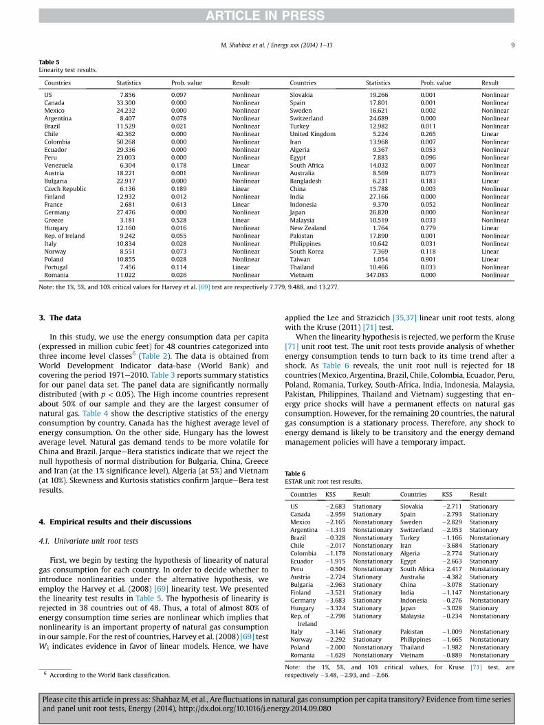
Table 5Linearity test results.

Countries Statistics Prob. value Result Countries Statistics Prob. value Result

US 7.856 0.097 Nonlinear Slovakia 19.266 0.001 NonlinearCanada 33.300 0.000 Nonlinear Spain 17.801 0.001 NonlinearMexico 24.232 0.000 Nonlinear Sweden 16.621 0.002 NonlinearArgentina 8.407 0.078 Nonlinear Switzerland 24.689 0.000 NonlinearBrazil 11.529 0.021 Nonlinear Turkey 12.982 0.011 NonlinearChile 42.362 0.000 Nonlinear United Kingdom 5.224 0.265 LinearColombia 50.268 0.000 Nonlinear Iran 13.968 0.007 NonlinearEcuador 29.336 0.000 Nonlinear Algeria 9.367 0.053 NonlinearPeru 23.003 0.000 Nonlinear Egypt 7.883 0.096 NonlinearVenezuela 6.304 0.178 Linear South Africa 14.032 0.007 NonlinearAustria 18.221 0.001 Nonlinear Australia 8.569 0.073 NonlinearBulgaria 22.917 0.000 Nonlinear Bangladesh 6.231 0.183 LinearCzech Republic 6.136 0.189 Linear China 15.788 0.003 NonlinearFinland 12.932 0.012 Nonlinear India 27.166 0.000 NonlinearFrance 2.681 0.613 Linear Indonesia 9.370 0.052 NonlinearGermany 27.476 0.000 Nonlinear Japan 26.820 0.000 NonlinearGreece 3.181 0.528 Linear Malaysia 10.519 0.033 NonlinearHungary 12.160 0.016 Nonlinear New Zealand 1.764 0.779 LinearRep. of Ireland 9.242 0.055 Nonlinear Pakistan 17.890 0.001 NonlinearItaly 10.834 0.028 Nonlinear Philippines 10.642 0.031 NonlinearNorway 8.551 0.073 Nonlinear South Korea 7.369 0.118 LinearPoland 10.855 0.028 Nonlinear Taiwan 1.054 0.901 LinearPortugal 7.456 0.114 Linear Thailand 10.466 0.033 NonlinearRomania 11.022 0.026 Nonlinear Vietnam 347.083 0.000 Nonlinear

Note: the 1%, 5%, and 10% critical values for Harvey et al. [69] test are respectively 7.779, 9.488, and 13.277.

Table 6ESTAR unit root test results.

Countries KSS Result Countries KSS Result


3. The data

In this study, we use the energy consumption data per capita(expressed in million cubic feet) for 48 countries categorized intothree income level classes6 (Table 2). The data is obtained fromWorld Development Indicator data-base (World Bank) andcovering the period 1971e2010. Table 3 reports summary statisticsfor our panel data set. The panel data are significantly normallydistributed (with p < 0.05). The High income countries representabout 50% of our sample and they are the largest consumer ofnatural gas. Table 4 show the descriptive statistics of the energyconsumption by country. Canada has the highest average level ofenergy consumption. On the other side, Hungary has the lowestaverage level. Natural gas demand tends to be more volatile forChina and Brazil. JarqueeBera statistics indicate that we reject thenull hypothesis of normal distribution for Bulgaria, China, Greeceand Iran (at the 1% significance level), Algeria (at 5%) and Vietnam(at 10%). Skewness and Kurtosis statistics confirm JarqueeBera testresults.

US �2.683 Stationary Slovakia �2.711 StationaryCanada �2.959 Stationary Spain �2.793 StationaryMexico �2.165 Nonstationary Sweden �2.829 StationaryArgentina �1.319 Nonstationary Switzerland �2.953 StationaryBrazil �0.328 Nonstationary Turkey �1.166 NonstationaryChile �2.017 Nonstationary Iran �3.684 StationaryColombia �1.178 Nonstationary Algeria �2.774 StationaryEcuador �1.915 Nonstationary Egypt �2.663 StationaryPeru �0.504 Nonstationary South Africa �2.417 NonstationaryAustria �2.724 Stationary Australia �4.382 StationaryBulgaria �2.963 Stationary China �3.078 StationaryFinland �3.521 Stationary India �1.147 NonstationaryGermany �3.683 Stationary Indonesia �0.276 NonstationaryHungary �3.324 Stationary Japan �3.028 StationaryRep. of

Ireland�2.798 Stationary Malaysia �0.234 Nonstationary

Italy �3.146 Stationary Pakistan �1.009 NonstationaryNorway �2.292 Stationary Philippines �1.665 NonstationaryPoland �2.000 Nonstationary Thailand �1.982 Nonstationary

4. Empirical results and their discussions

4.1. Univariate unit root tests

First, we begin by testing the hypothesis of linearity of naturalgas consumption for each country. In order to decide whether tointroduce nonlinearities under the alternative hypothesis, weemploy the Harvey et al. (2008) [69] linearity test. We presentedthe linearity test results in Table 5. The hypothesis of linearity isrejected in 38 countries out of 48. Thus, a total of almost 80% ofenergy consumption time series are nonlinear which implies thatnonlinearity is an important property of natural gas consumptionin our sample. For the rest of countries, Harvey et al. (2008) [69] testWl indicates evidence in favor of linear models. Hence, we have

6 According to the World Bank classification.


applied the Lee and Strazicich [35,37] linear unit root tests, alongwith the Kruse (2011) [71] test.

When the linearity hypothesis is rejected, we perform the Kruse[71] unit root test. The unit root tests provide analysis of whetherenergy consumption tends to turn back to its time trend after ashock. As Table 6 reveals, the unit root null is rejected for 18countries (Mexico, Argentina, Brazil, Chile, Colombia, Ecuador, Peru,Poland, Romania, Turkey, South-Africa, India, Indonesia, Malaysia,Pakistan, Philippines, Thailand and Vietnam) suggesting that en-ergy price shocks will have a permanent effects on natural gasconsumption. However, for the remaining 20 countries, the naturalgas consumption is a stationary process. Therefore, any shock toenergy demand is likely to be transitory and the energy demandmanagement policies will have a temporary impact.

Romania �1.629 Nonstationary Vietnam �0.889 Nonstationary

Note: the 1%, 5%, and 10% critical values, for Kruse [71] test, arerespectively �3.48, �2.93, and �2.66.


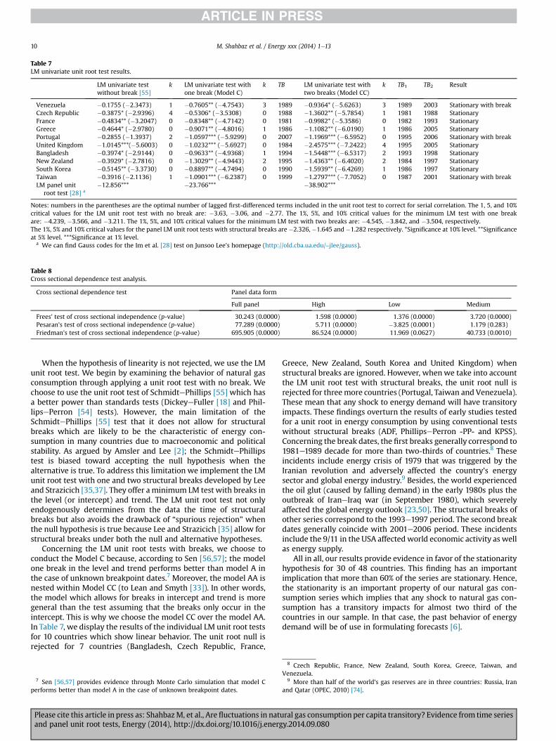
Table 7LM univariate unit root test results.

LM univariate testwithout break [55]

k LM univariate test withone break (Model C)

k TB LM univariate test withtwo breaks (Model CC)

k TB1 TB2 Result

Venezuela �0.1755 (�2.3473) 1 �0.7605** (�4.7543) 3 1989 �0.9364* (�5.6263) 3 1989 2003 Stationary with breakCzech Republic �0.3875* (�2.9396) 4 �0.5306* (�3.5308) 0 1988 �1.3602** (�5.7854) 1 1981 1988 StationaryFrance �0.4834** (�3.2047) 0 �0.8348** (�4.7142) 0 1981 �0.9982* (�5.3586) 0 1982 1993 StationaryGreece �0.4644* (�2.9780) 0 �0.9071** (�4.8016) 1 1986 �1.1082** (�6.0190) 1 1986 2005 StationaryPortugal �0.2855 (�1.3937) 2 �1.0597*** (�5.9299) 0 2007 �1.1969*** (�6.5952) 0 1995 2006 Stationary with breakUnited Kingdom �1.0145***(�5.6003) 0 �1.0232*** (�5.6927) 0 1984 �2.4575*** (�7.2422) 4 1995 2005 StationaryBangladesh �0.3974* (�2.9144) 0 �0.9633** (�4.9368) 1 1994 �1.5448*** (�6.5317) 2 1993 1998 StationaryNew Zealand �0.3929* (�2.7816) 0 �1.3029** (�4.9443) 2 1995 �1.4363** (�6.4020) 2 1984 1997 StationarySouth Korea �0.5145** (�3.3730) 0 �0.8897** (�4.7494) 0 1990 �1.5939** (�6.4269) 1 1986 1997 StationaryTaiwan �0.3916 (�2.1136) 1 �1.0901*** (�6.2387) 0 1999 �1.2797*** (�7.7052) 0 1987 2001 Stationary with breakLM panel unit

root test [28] a�12.856*** �23.766*** �38.902***

Notes: numbers in the parentheses are the optimal number of lagged first-differenced terms included in the unit root test to correct for serial correlation. The 1, 5, and 10%critical values for the LM unit root test with no break are: �3.63, �3.06, and �2.77. The 1%, 5%, and 10% critical values for the minimum LM test with one breakare: �4.239, �3.566, and �3.211. The 1%, 5%, and 10% critical values for the minimum LM test with two breaks are: �4.545, �3.842, and �3.504, respectively.The 1%, 5% and 10% critical values for the panel LM unit root tests with structural breaks are �2.326, �1.645 and �1.282 respectively. *Significance at 10% level. **Significanceat 5% level. ***Significance at 1% level.

a We can find Gauss codes for the Im et al. [28] test on Junsoo Lee's homepage (http://old.cba.ua.edu/~jlee/gauss).

Table 8Cross sectional dependence test analysis.

Cross sectional dependence test Panel data form

Full panel High Low Medium

Frees' test of cross sectional independence (p-value) 30.243 (0.0000) 1.598 (0.0000) 1.376 (0.0000) 3.720 (0.0000)Pesaran's test of cross sectional independence (p-value) 77.289 (0.0000) 5.711 (0.0000) �3.825 (0.0001) 1.179 (0.283)Friedman's test of cross sectional independence (p-value) 695.905 (0.0000) 86.524 (0.0000) 11.969 (0.0627) 40.733 (0.0010)


When the hypothesis of linearity is not rejected, we use the LMunit root test. We begin by examining the behavior of natural gasconsumption through applying a unit root test with no break. Wechoose to use the unit root test of SchmidtePhillips [55] which hasa better power than standards tests (DickeyeFuller [18] and Phil-lipsePerron [54] tests). However, the main limitation of theSchmidtePhillips [55] test that it does not allow for structuralbreaks which are likely to be the characteristic of energy con-sumption in many countries due to macroeconomic and politicalstability. As argued by Amsler and Lee [2]; the SchmidtePhillipstest is biased toward accepting the null hypothesis when thealternative is true. To address this limitation we implement the LMunit root test with one and two structural breaks developed by Leeand Strazicich [35,37]. They offer a minimum LM test with breaks inthe level (or intercept) and trend. The LM unit root test not onlyendogenously determines from the data the time of structuralbreaks but also avoids the drawback of “spurious rejection” whenthe null hypothesis is true because Lee and Strazicich [35] allow forstructural breaks under both the null and alternative hypotheses.

Concerning the LM unit root tests with breaks, we choose toconduct the Model C because, according to Sen [56,57]; the modelone break in the level and trend performs better than model A inthe case of unknown breakpoint dates.7 Moreover, the model AA isnested within Model CC (to Lean and Smyth [33]). In other words,the model which allows for breaks in intercept and trend is moregeneral than the test assuming that the breaks only occur in theintercept. This is why we choose the model CC over the model AA.In Table 7, we display the results of the individual LM unit root testsfor 10 countries which show linear behavior. The unit root null isrejected for 7 countries (Bangladesh, Czech Republic, France,

7 Sen [56,57] provides evidence through Monte Carlo simulation that model Cperforms better than model A in the case of unknown breakpoint dates.


Greece, New Zealand, South Korea and United Kingdom) whenstructural breaks are ignored. However, whenwe take into accountthe LM unit root test with structural breaks, the unit root null isrejected for threemore countries (Portugal, Taiwan and Venezuela).These mean that any shock to energy demand will have transitoryimpacts. These findings overturn the results of early studies testedfor a unit root in energy consumption by using conventional testswithout structural breaks (ADF, PhillipsePerron -PP- and KPSS).Concerning the break dates, the first breaks generally correspond to1981e1989 decade for more than two-thirds of countries.8 Theseincidents include energy crisis of 1979 that was triggered by theIranian revolution and adversely affected the country's energysector and global energy industry.9 Besides, the world experiencedthe oil glut (caused by falling demand) in the early 1980s plus theoutbreak of IraneIraq war (in September 1980), which severelyaffected the global energy outlook [23,50]. The structural breaks ofother series correspond to the 1993e1997 period. The second breakdates generally coincide with 2001e2006 period. These incidentsinclude the 9/11 in the USA affected world economic activity as wellas energy supply.

All in all, our results provide evidence in favor of the stationarityhypothesis for 30 of 48 countries. This finding has an importantimplication that more than 60% of the series are stationary. Hence,the stationarity is an important property of our natural gas con-sumption series which implies that any shock to natural gas con-sumption has a transitory impacts for almost two third of thecountries in our sample. In that case, the past behavior of energydemand will be of use in formulating forecasts [6].

8 Czech Republic, France, New Zealand, South Korea, Greece, Taiwan, andVenezuela.

9 More than half of the world's gas reserves are in three countries: Russia, Iranand Qatar (OPEC, 2010) [74].


http://old.cba.ua.edu/%7Ejlee/gauss

Table 9Panel data unit root analysis.a

Types of test statistic Test statistic 1% CV 5 % CV 10 % CV

First generation of panel unit root tests: full panelLLC test statistic �8.3744 �2.3263 �1.6449 �1.2816IPS test statistic �11.5931 �2.3263 �1.6449 �1.2816MW test statistic 290.9159 133.4756 122.1077 116.3152Choi test statistic 14.0668 2.3263 1.6449 1.2816

Second-generation panel unit root tests: full panelMoon Perron1 statistic

(ta_bar statistic)�2.8608 �2.3263 �1.6449 �1.2816

Moon Perron2 statistic(tb_bar statistic)

�2.4549 �2.3263 �1.6449 �1.2816

Pesaran test [53] statistic �6.084 �2.7260 �2.6077 �2.5441Choi test statistic (Pm) 13.3044 2.3263 1.6449 1.2816Choi test statistic (Z) �9.6374 �2.3263 �1.6449 �1.2816Choi test statistic (Lstar) �10.3160 �2.3263 �1.6449 �1.2816

First generation of panel unit root tests: high income panelLLC test statistic �11.0250 �2.3263 �1.6449 �1.2816IPS test statistic �11.8060 �2.3263 �1.6449 �1.2816MW test statistic 103.068 71.2014 62.8296 58.6405Choi test statistic 10.7137 2.3263 1.6449 1.2816

Second-generation panel unit root tests: high income panelMoon Perron1 statistic

(ta_bar statistic)�8.1245 �2.3263 �1.6449 �1.2816


�5.7333 �2.3263 �1.6449 �1.2816

Pesaran test [53] �7.773 �2.8749 �2.7148 �2.6298Choi test statistic (Pm) 14.4759 2.3263 1.6449 1.2816Choi test statistic (Z) �8.4181 �2.3263 �1.6449 �1.2816Choi test statistic (Lstar) �10.0702 �2.3263 �1.6449 �1.2816

First generation of panel unit root tests: low income panelLLC test statistic �1.4327 �2.3263 �1.6449 �1.2816IPS test statistic �1.6069 �2.3263 �1.6449 �1.2816MW test statistic 33.8849 29.1412 23.6847 21.0641Choi test statistic 3.7579 2.3263 1.6449 1.2816

Second-generation panel unit root tests: low income panelMoon Perron1 statistic

(ta_bar statistic)�5.2348 �2.3263 �1.6449 �1.2816


�4.3906 �2.3263 �1.6449 �1.2816

Pesaran test [53] �2.243 �3.0705 �2.8353 �2.7264Choi test statistic (Pm) 3.5782 2.3263 1.6449 1.2816Choi test statistic (Z) �1.6218 �2.3263 �1.6449 �1.2816Choi test statistic (Lstar) �2.1255 �2.3263 �1.6449 �1.2816LLC test statistic �8.1364 �2.3263 �1.6449 �1.2816IPS test statistic �8.5498 �2.3263 �1.6449 �1.2816MW test statistic 78.040 56.0609 48.6023 44.9031Choi test statistic 8.5170 2.3263 1.6449 1.2816

Second-generation panel unit root tests: middle income panelMoon Perron1 statistic

(ta_bar statistic)�9.1880 �2.3263 �1.6449 �1.2816


�3.3473 �2.3263 �1.6449 �1.2816

Pesaran test [53] �4.318 �2.9330 �2.7534 �2.6676Choi test statistic (Pm) 4.9544 2.3263 1.6449 1.2816Choi test statistic (Z) �3.9529 �2.3263 �1.6449 �1.2816Choi test statistic (Lstar) �4.1222 �2.3263 �1.6449 �1.2816

a We can find Matlab codes for the panel unit root test on Christophe Hurlin'shomepage (http://www.univ-orleans.fr/deg/masters/ESA/CH/churlin_R.htm).

Table 10Panel unit root test which allow for structural breaks [28].

Panels No break One break Two breaks

Full panel �44.195*** �51.699*** �105.419***High income panel �29.581*** �37.055*** �47.990***Middle income panel �24.044*** �41.075*** �44.554***Low income panel �8.738*** �21.171*** �26.743***

Note: the 1%, 5% and 10% critical values for the panel LM unit root tests withstructural breaks are �2.326, �1.645 and �1.282 respectively. *Significance at 10%level. **Significance at 5% level. ***Significance at 1% level.


4.2. Panel data unit root tests

To make the analysis robust, the results of panel data unit roottests should be compared with those obtained with univariate unitroot tests. In order to check the degree of integration of our series,we have thus carried out a panel data unit root tests for thefollowing panels: the full countries panel (48 countries), high


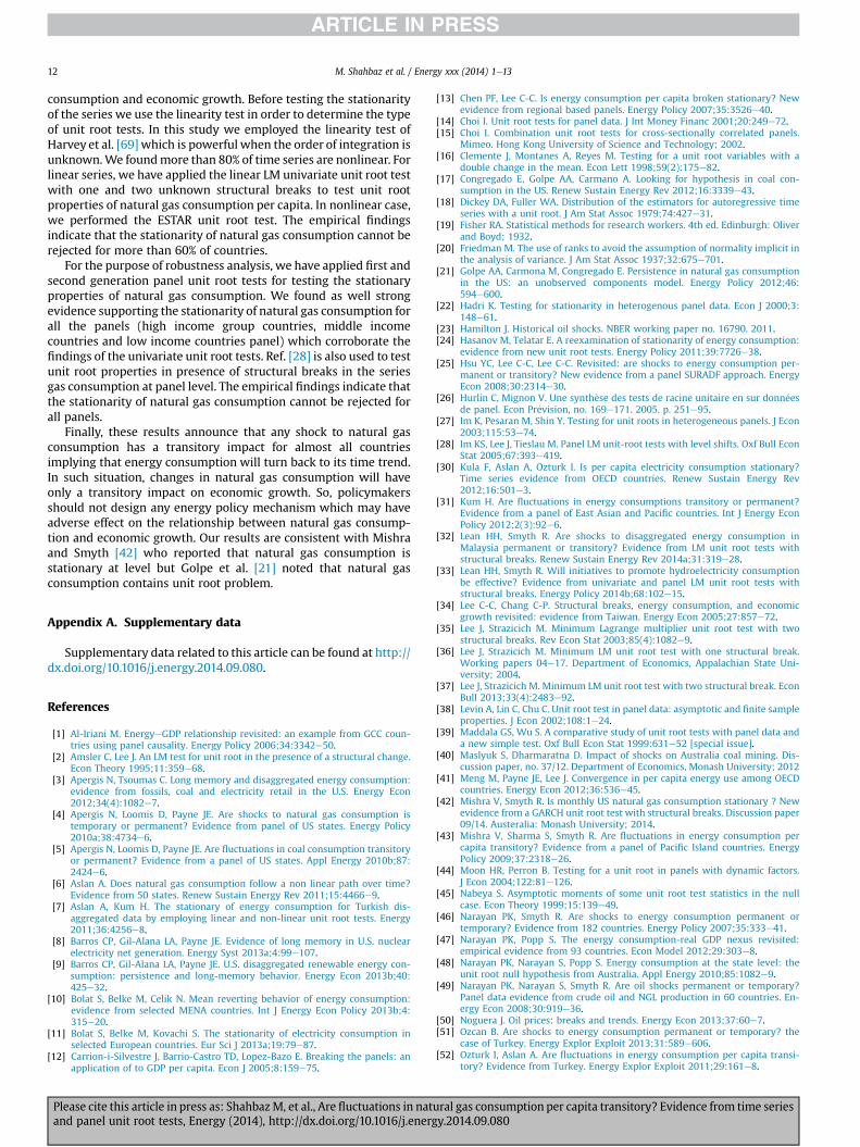
income countries panel (23 countries), middle income countriespanel (18 countries) and low income countries panel (7 countries).However, before examining the order of integration of our series wehave to test the assumption of cross sectional dependence in panelswhich can arise due to a multiplicity of factors such as unobservedor/and omitted common factors, spatial correlations, economicdistance and common unobserved shocks. Three tests for crosssection dependence have been used in our study namely, Pesaran's[75] cross sectional dependence test, Friedman's [20] statistic andthe test statistic proposed by Frees [67]. Table 8 reveals that the nullhypothesis of no cross-sectional dependence is largely rejected at1% and 10% respectively leading us to conclude the dependence inour data. This finding highlights the importance of taking into ac-count cross-section dependence when investigating the energyconsumption stationarity.

Despite the presence of cross-sectional dependence weemployed a series of panel unit root tests that assume crosssectional independence (the so called first generation panel dataunit root tests) and cross-sectional dependence (second generationpanel data unit root tests). All unit root tests with no exceptionsuppose no-stationarity under the null hypothesis. However, thesetests do not allow for structural breaks. For this reason wecompleted our analysis by employing the Lagrange Multiplier (LM)panel unit root test with level breaks [28]. The null hypothesis ofthe LM panel test is that all series contain unit roots, with thealternative that some of the series in the panel are stationary.

The results of panel unit root tests reported in Table 9 indicatethat null hypothesis of unit root test in natural gas consumption percapita series is rejected by both first and second generation tests forthe full panel, high income countries panel, middle income coun-tries and low income countries. The results from the Im, Lee andTieslau [28] test (Table 10), allowing for structural breaks, corrob-orate the findings of both the first and second generation panel dataunit root tests. The unit root is rejected for each panel in the oneand two breaks. The LM panel test provides as well strong evidencein favor of stationarity of natural gas demand. This leads us toconclude that the energy consumption is stationary in each of thefour panels. These findings imply that exogenous shocks have atemporary effect in energy demand for thewhole countries sample.

Finally, for comparison purposes, we applied panel LM unit roottest of Im et al. [28] for linear time series. The results are reported atthe bottom of Table 7 where we found evidence in support of sta-tionarity for the panel of countries that follow a linear behavior.This finding indicates that natural gas consumption for thesecountries will return back to its trend path over time and it mightbe possible to forecast future projections in reference to past energyconsumption.

5. Concluding remarks and policy implications

The empirical investigation of unit root properties of natural gasconsumption is helpful inmodeling energy-growth nexus as well asdetecting the direction of causality between natural gas


http://www.univ-orleans.fr/deg/masters/ESA/CH/churlin_R.htm


consumption and economic growth. Before testing the stationarityof the series we use the linearity test in order to determine the typeof unit root tests. In this study we employed the linearity test ofHarvey et al. [69] which is powerful when the order of integration isunknown.We foundmore than 80% of time series are nonlinear. Forlinear series, we have applied the linear LM univariate unit root testwith one and two unknown structural breaks to test unit rootproperties of natural gas consumption per capita. In nonlinear case,we performed the ESTAR unit root test. The empirical findingsindicate that the stationarity of natural gas consumption cannot berejected for more than 60% of countries.

For the purpose of robustness analysis, we have applied first andsecond generation panel unit root tests for testing the stationaryproperties of natural gas consumption. We found as well strongevidence supporting the stationarity of natural gas consumption forall the panels (high income group countries, middle incomecountries and low income countries panel) which corroborate thefindings of the univariate unit root tests. Ref. [28] is also used to testunit root properties in presence of structural breaks in the seriesgas consumption at panel level. The empirical findings indicate thatthe stationarity of natural gas consumption cannot be rejected forall panels.

Finally, these results announce that any shock to natural gasconsumption has a transitory impact for almost all countriesimplying that energy consumption will turn back to its time trend.In such situation, changes in natural gas consumption will haveonly a transitory impact on economic growth. So, policymakersshould not design any energy policy mechanism which may haveadverse effect on the relationship between natural gas consump-tion and economic growth. Our results are consistent with Mishraand Smyth [42] who reported that natural gas consumption isstationary at level but Golpe et al. [21] noted that natural gasconsumption contains unit root problem.

Appendix A. Supplementary data

Supplementary data related to this article can be found at http://dx.doi.org/10.1016/j.energy.2014.09.080.

References

[1] Al-Iriani M. EnergyeGDP relationship revisited: an example from GCC coun-tries using panel causality. Energy Policy 2006;34:3342e50.

[2] Amsler C, Lee J. An LM test for unit root in the presence of a structural change.Econ Theory 1995;11:359e68.

[3] Apergis N, Tsoumas C. Long memory and disaggregated energy consumption:evidence from fossils, coal and electricity retail in the U.S. Energy Econ2012;34(4):1082e7.

[4] Apergis N, Loomis D, Payne JE. Are shocks to natural gas consumption istemporary or permanent? Evidence from panel of US states. Energy Policy2010a;38:4734e6.

[5] Apergis N, Loomis D, Payne JE. Are fluctuations in coal consumption transitoryor permanent? Evidence from a panel of US states. Appl Energy 2010b;87:2424e6.

[6] Aslan A. Does natural gas consumption follow a non linear path over time?Evidence from 50 states. Renew Sustain Energy Rev 2011;15:4466e9.

[7] Aslan A, Kum H. The stationary of energy consumption for Turkish dis-aggregated data by employing linear and non-linear unit root tests. Energy2011;36:4256e8.

[8] Barros CP, Gil-Alana LA, Payne JE. Evidence of long memory in U.S. nuclearelectricity net generation. Energy Syst 2013a;4:99e107.

[9] Barros CP, Gil-Alana LA, Payne JE. U.S. disaggregated renewable energy con-sumption: persistence and long-memory behavior. Energy Econ 2013b;40:425e32.

[10] Bolat S, Belke M, Celik N. Mean reverting behavior of energy consumption:evidence from selected MENA countries. Int J Energy Econ Policy 2013b;4:315e20.

[11] Bolat S, Belke M, Kovachi S. The stationarity of electricity consumption inselected European countries. Eur Sci J 2013a;19:79e87.

[12] Carrion-i-Silvestre J, Barrio-Castro TD, Lopez-Bazo E. Breaking the panels: anapplication of to GDP per capita. Econ J 2005;8:159e75.


[13] Chen PF, Lee C-C. Is energy consumption per capita broken stationary? Newevidence from regional based panels. Energy Policy 2007;35:3526e40.

[14] Choi I. Unit root tests for panel data. J Int Money Financ 2001;20:249e72.[15] Choi I. Combination unit root tests for cross-sectionally correlated panels.

Mimeo. Hong Kong University of Science and Technology; 2002.[16] Clemente J, Montanes A, Reyes M. Testing for a unit root variables with a

double change in the mean. Econ Lett 1998;59(2):175e82.[17] Congregado E, Golpe AA, Carmano A. Looking for hypothesis in coal con-

sumption in the US. Renew Sustain Energy Rev 2012;16:3339e43.[18] Dickey DA, Fuller WA. Distribution of the estimators for autoregressive time

series with a unit root. J Am Stat Assoc 1979;74:427e31.[19] Fisher RA. Statistical methods for research workers. 4th ed. Edinburgh: Oliver

and Boyd; 1932.[20] Friedman M. The use of ranks to avoid the assumption of normality implicit in

the analysis of variance. J Am Stat Assoc 1937;32:675e701.[21] Golpe AA, Carmona M, Congregado E. Persistence in natural gas consumption

in the US: an unobserved components model. Energy Policy 2012;46:594e600.

[22] Hadri K. Testing for stationarity in heterogenous panel data. Econ J 2000;3:148e61.

[23] Hamilton J. Historical oil shocks. NBER working paper no. 16790. 2011.[24] Hasanov M, Telatar E. A reexamination of stationarity of energy consumption:

evidence from new unit root tests. Energy Policy 2011;39:7726e38.[25] Hsu YC, Lee C-C, Lee C-C. Revisited: are shocks to energy consumption per-

manent or transitory? New evidence from a panel SURADF approach. EnergyEcon 2008;30:2314e30.

[26] Hurlin C, Mignon V. Une synth�ese des tests de racine unitaire en sur donn�eesde panel. Econ Pr�evision, no. 169e171. 2005. p. 251e95.

[27] Im K, Pesaran M, Shin Y. Testing for unit roots in heterogeneous panels. J Econ2003;115:53e74.

[28] Im KS, Lee J, Tieslau M. Panel LM unit-root tests with level shifts. Oxf Bull EconStat 2005;67:393e419.

[30] Kula F, Aslan A, Ozturk I. Is per capita electricity consumption stationary?Time series evidence from OECD countries. Renew Sustain Energy Rev2012;16:501e3.

[31] Kum H. Are fluctuations in energy consumptions transitory or permanent?Evidence from a panel of East Asian and Pacific countries. Int J Energy EconPolicy 2012;2(3):92e6.

[32] Lean HH, Smyth R. Are shocks to disaggregated energy consumption inMalaysia permanent or transitory? Evidence from LM unit root tests withstructural breaks. Renew Sustain Energy Rev 2014a;31:319e28.

[33] Lean HH, Smyth R. Will initiatives to promote hydroelectricity consumptionbe effective? Evidence from univariate and panel LM unit root tests withstructural breaks. Energy Policy 2014b;68:102e15.

[34] Lee C-C, Chang C-P. Structural breaks, energy consumption, and economicgrowth revisited: evidence from Taiwan. Energy Econ 2005;27:857e72.

[35] Lee J, Strazicich M. Minimum Lagrange multiplier unit root test with twostructural breaks. Rev Econ Stat 2003;85(4):1082e9.

[36] Lee J, Strazicich M. Minimum LM unit root test with one structural break.Working papers 04e17. Department of Economics, Appalachian State Uni-versity; 2004.

[37] Lee J, Strazicich M. Minimum LM unit root test with two structural break. EconBull 2013;33(4):2483e92.

[38] Levin A, Lin C, Chu C. Unit root test in panel data: asymptotic and finite sampleproperties. J Econ 2002;108:1e24.

[39] Maddala GS, Wu S. A comparative study of unit root tests with panel data anda new simple test. Oxf Bull Econ Stat 1999:631e52 [special issue].

[40] Maslyuk S, Dharmaratna D. Impact of shocks on Australia coal mining. Dis-cussion paper, no. 37/12. Department of Economics, Monash University; 2012

[41] Meng M, Payne JE, Lee J. Convergence in per capita energy use among OECDcountries. Energy Econ 2012;36:536e45.

[42] Mishra V, Smyth R. Is monthly US natural gas consumption stationary ? Newevidence from a GARCH unit root test with structural breaks. Discussion paper09/14. Austeralia: Monash University; 2014.

[43] Mishra V, Sharma S, Smyth R. Are fluctuations in energy consumption percapita transitory? Evidence from a panel of Pacific Island countries. EnergyPolicy 2009;37:2318e26.

[44] Moon HR, Perron B. Testing for a unit root in panels with dynamic factors.J Econ 2004;122:81e126.

[45] Nabeya S. Asymptotic moments of some unit root test statistics in the nullcase. Econ Theory 1999;15:139e49.

[46] Narayan PK, Smyth R. Are shocks to energy consumption permanent ortemporary? Evidence from 182 countries. Energy Policy 2007;35:333e41.

[47] Narayan PK, Popp S. The energy consumption-real GDP nexus revisited:empirical evidence from 93 countries. Econ Model 2012;29:303e8.

[48] Narayan PK, Narayan S, Popp S. Energy consumption at the state level: theunit root null hypothesis from Australia. Appl Energy 2010;85:1082e9.

[49] Narayan PK, Narayan S, Smyth R. Are oil shocks permanent or temporary?Panel data evidence from crude oil and NGL production in 60 countries. En-ergy Econ 2008;30:919e36.

[50] Noguera J. Oil prices: breaks and trends. Energy Econ 2013;37:60e7.[51] Ozcan B. Are shocks to energy consumption permanent or temporary? the

case of Turkey. Energy Explor Exploit 2013;31:589e606.[52] Ozturk I, Aslan A. Are fluctuations in energy consumption per capita transi-

tory? Evidence from Turkey. Energy Explor Exploit 2011;29:161e8.




http://refhub.elsevier.com/S0360-5442(14)01147-5/sref1







































































































































































[53] Pesaran H. A simple panel unit root test in the presence of cross sectiondependence. J Appl Econ 2007;22(2):265e312.

[54] Phillips PCB, Perron P. Testing for a unit root in time series regression. Bio-metrika 1988;75:335e46.

[55] Schmidt P, Phillips PCB. LM tests for a unit root in the presence of deter-ministic trends. Oxf Bull Econ Stat 1992;54:257e87.

[56] Sen A. On unit root tests when the alternative is a trend break stationaryprocess. J Bus Econ Stat 2003a;21:174e84.

[57] Sen A. Some aspects of the unit root testing methodology with application toreal per-capita GDP. Manuscript. Cincinnati, OH: Xavier University; 2003b.

[58] Shahbaz M, Tiwari AV, Farrok AJ, Ozturk I. Are fluctuations in coal con-sumption per capita temporary? Evidence from developed and developingcountries. Renew Sustain Energy Rev 2014;33:96e101.

[59] Shahbaz M, Tiwari AV, Ozturk I, Farrok AJ. Are fluctuations in electricityconsumption per capita transitory? Evidence from developed and developingeconomies. Renew Sustain Energy Rev 2013;28:551e4.

[60] Smyth R. Are fluctuations in energy variables permanent or temporary? Asurvey of the literature on the integration properties of energy consumptionand production. Appl Energy 2013;104:371e8.

[61] Soytas U, Sari R. Can China contribute more to the fight against globalwarming? J Policy Model 2006;28:837e46.

[62] Zachariadis T, Pashouritdou N. An empirical analysis of electricity consump-tion in Cyprus. Energy Econ 2007;29:183e98.

[63] Zevot E, Andrews D. Further evidence of the great crash, the oil price shockand the unit root hypothesis. J Bus Econ Stat 1992;10:251e70.

[64] Abadir KM, Distaso W. Testing joint hypotheses when one of the alternativesis one-sided. Journal of Econometrics 2007;140:695e718.


[65] Agnolucci P, Venn A. Industrial energy intensities in the UK: is there adeterministic or stochastic difference among sectors? Applied Economics2011;43:1447e62.

[66] BP. BP. Energy outlook. 2012. London: UK.[67] Frees EW. Assessing cross-sectional correlations in panel data. Journal of

Econometrics 1995;69:393e414.[68] Harvey DI, Leybourne SJ. Testing for time series linearity. Econometrics

Journal 2007;10:149e65.[69] Harvey DI, Leybourne SJ, Xiao B. A powerful test for linearity when the order

of integration is unknown. Studies in Nonlinear Dynamics & Econometrics2008:12. Article 2.

[70] Kapetanios G, Shin Y, Snell A. Testing for a unit root in the nonlinear STARframework. Journal of Econometrics 2003;112:359e79.

[71] Kruse R. A new unit root test against ESTAR based on a class of modifiedstatistics. Statistical Papers 2011;52:71e85.

[72] Narayan PK, Smyth R. Electricity consumption, employment and real incomein Australia: evidence from multivariate Granger causality tests. Energy Policy2005;33:1109e16.

[73] Narayan PK, Popp S. The energy consumption-real GDP nexus revisited:empirical evidence from 93 countries. Economic Modeling 2012;29:303e8.

[74] OPEC Annual Statistical Bulletin. 2010. www.opec.org.[75] Pesaran MH. General diagnostic tests for cross section dependence in panels.

University of Cambridge; 2004. Faculty of Economics, Cambridge WorkingPapers in Economics No. 0435.

[76] World Energy Outlook. 2011. www.worldenergyoutlook.org.[77] BP. BP. Statistical review of world energy. June 2013. London: UK.




































































http://www.opec.org




http://www.worldenergyoutlook.org


Are fluctuations in natural gas consumption per capita transitory? Evidence from time series and...

Documents

Transcript of Are fluctuations in natural gas consumption per capita transitory? Evidence from time series and...