Insect olfaction as an information filter for chemo-analytical ...
Upload
maduracollegeCategory
view
2download
0
Copyright © 2014 by Modern Scientific Press Company, Florida, USA
International Journal of Modern Mathematical Sciences, 2014, 9(3): 173-197
International Journal of Modern Mathematical Sciences
Journal homepage:www.ModernScientificPress.com/Journals/ijmms.aspx
ISSN:2166-286X
Florida, USA
Article
Approximate Analytical Solution of Chemo Attractant Gradient
Sensing Based on Receptor-regulated Membrane Phospholipid
Signaling Dynamics
K. M. Dharmalingam*, S. Kalaiselvi and V. Ananthaswamy
Department of Mathematics, The Madura College, Madurai-625011, Tamil Nadu, India
* Author to whom correspondence should be addressed: Email: [email protected]
Article history: Received 5 January 2014, Accepted 3 March 2014, Published 10 March 2014.
Abstract: In this paper the analytical solution of steady state non-linear boundary value
problem in phosphoinositide dynamics is discussed. The analytical expression of the
receptor desensitization and the reaction-diffusion process of the phosphoinositide can be
obtained using Homotopy perturbation method (HPM) for various values of the relevant
parameters. In this study, the analytical results have been compared with perturbation
method and which showed that, the present approach has less computational aspect and are
applicable for solving other non-linear boundary value problem.
Keywords: Cell migration; Chemotaxix; Phosophoinositides; Non-linear reaction-diffusion
equations; Homotopy perturbation method; Numerical simulation.
Mathematics Subject Classification (2000): Mathematical modeling and non-linear
differential equation.
1. Introduction
Cellular migration is a coordinated process that resultsfrom the interaction of specific cell
surface receptorswith ligands of the extracellular matrix ~ECM. Usingwell-controlled, stable, ligand
substrates, a number ofligand properties have been shown to affect activation ofcellmotility, including,
for example, ligand surface concentration, strength of ligand–receptor adhesion, degreeof receptor

Int. J. Modern Math. Sci. 2014, 9(3): 173-197
Copyright © 2014 by Modern Scientific Press Company, Florida, USA
174
occupancy by the ligand, and ligand affinity[1].The general consensus that, the synthesis of PtdIns is
constitutive and which is the centre of major regulatory mechanisms on the subsequent generationof
the polyphosphoinositides[2]. Actin reorganization is a bidirectional process that orchestratescomplex
cellular events such as, cell migration, neurite extension and bud growth in yeast.The WASP family of
scaffoldingproteins, WASP, N-WASP and WAVE, participate in theseprocesses by relaying signals
from Rho-family GTPases to the actin remodeling machinery [3].Precise regulation of protein-protein
interaction is criticalfor determining the wiring of cellular signaling pathways [4].
Receptors are responsible for transmitting information about theexternal environment to the
cell internum, and therefore theirmechanism of activation and action must be well characterizedbefore
the details of the intracellular networks can be analyzedand modeled mathematically (signaling
network).Two-dimensional molecular gradients in cell membranesare also relevant in signal
transduction. Most signalingpathways involve specific membrane-associated intermediatesthat are
produced or activated through recruitment ofsignaling enzymes to the plasma membrane. Gradients in
thedensity of specific membrane lipids or activated lipidanchoredproteins may form on the nanometer
scale if therates of the reactions that produce them are rapid enough tobe limited by lateral diffusion
and gradients on longer length scales can form whenthe extracellular stimulus is spatially confined or
otherwiseorganized [5].
A fundamental problem of directional sensingis its exquisite sensitivity. Even in the presence
of relativelyshallow chemoattractant gradients, cell projections are extendedprecisely in the region
exposed to the highest chemoattractant concentration. This reflects the existence of a mechanism
foramplifying the external signal.A key problem in directional sensing is the elucidationof the
mechanism underlying the formation of ahighly polarized distribution of actin polymers in responseto
a mild gradient. Indeed, chemoattractant gradients imposed in the extracellular space are often
quitesmall ~1%–2% concentration change over the length of the cell.If a chemo-attractant gradient is
imposed on the cells,GFP–PH migrates within 5–10 s to the leading edge ofthe cell, and persistently
maintains this polarized distribution.This stands in sharp contrast to the results obtainedin response to a
uniform chemo-attractant concentration profile [6].Systems biology modeling of signal transduction
pathwaystraditionally employs ordinary differential equations,deterministic models based on the
assumptions of spatial homogeneity. Cell signaling is an essential, ubiquitous process thatliving
systems use to respond to the environment [7]. Distinguishing modes of Eukaryotic gradient sensing is
developed by Skupsky et.al. [8]. During directional gradient sensing, eukaryotic cells suchas
Dictyostelium and neutrophils exhibit extraordinarysensitivity to external chemical gradients.Shannon
K Hughes-Alford et.al. discussed quantitative analysis of gradient sensing [9]. Noritaka Masaki et.al.
proposed single cell level analysis of PDE expression in Dictyostelium [10].

Int. J. Modern Math. Sci. 2014, 9(3): 173-197
Copyright © 2014 by Modern Scientific Press Company, Florida, USA
175
The analytical expression of Ligand bound sensitive receptors, membrane phosphoinositicides,
stored phosphoinositicides and cytosolic inosilol phosphates are presented. These concentrations are
derived using Homotopy perturbation method.
2. Mathematical Formulation of the Problem
To simulate the experiments, it is assumed that before the cell is subjected to a chemoattractant
perturbation ),0( t it is in a homogeneous steady state, ),0,,,( 10 ippr s corresponding to a
uniform chemoattractant concentration, say, l . At ,0t the cell is perturbated by exposing it to a
new chemoattractant concentration profile, .)(l The reduced equations are
2
102
2101010,01
10
10
1
1
r
R
DrKekek
KelKt
r rdta
dl
(1)
2
2
2
2
10
p
R
Dpkcipkpprk
t
p p
pprsf (2)
2
2
2
2
10
sp
pprsfs p
R
Dpkcipkpprk
t
ps (3)
2
2
2
2
10
i
R
Dikcipkpprks
t
i iiirsf (4)
Here, ipspr DDDD and,, denote the lateral diffusivities of ,and,,10 IPPR s and R denotes the cell
radius. The factor s , denoting membrane length per unit cell area, is required since synthesis and
removal rates of P are based on the length of the plasma membrane. Since the cell is circular,
concentrations and fluxes must be equal at 20 and . Thus, we require the periodic boundary
conditions
0,),2(),0(
),,2(),0(
t
txtxtxtx
(5)
where .,,,10 ipprx s The initial conditions for the reduced equations are
iippppp
KelK
KelKrrt ts
dl
dl ,,,1
1;0
10
10
1010
(6)
They reflect the assumptions that:
(1) The total amount of phosphoinositide in the membrane and the endoplasmic reticulum is
conserved, so that the average phosphoinositide concentration, denoted tp is constant.
(2) Information concerning the chemoattractant concentration profile imposed at 0t , namely,
l , is transmitted to the receptors instantaneously. Thus, 10r changes during this rapid
process, but iandpp s ,, remain unchanged.

Int. J. Modern Math. Sci. 2014, 9(3): 173-197
Copyright © 2014 by Modern Scientific Press Company, Florida, USA
176
By introducing the dimensionless variables
10
10
10r
r ,
tp
p ,
t
ss
p
p , ι
tsp
i ,
1416.3*2
,
tr spk
t
1
(7)
and dimensionless parameters
tr spk
k01
01 ,
10
,
,r
e ta
ta , lK
l ,
10K
ed
d , tr
rr
spk
CD 2
(8)
tr
tf
fspk
prk 2
10
, tr
tp
pspk
pc ,
tr
p
pspk
k ,
tr
p
pspk
CD 2
(9)
tr
sp
pspk
CD
s
2
,
tr
tii
spk
spc ,
tr
ii
spk
k ,
tr
ii
spk
CD 2
, lK
l
(10)
tp
p ,
t
ss
p
p , ι-
tsp
i
(11)
Where C denotes the circumference of the cell. Thus we get the dimensionless equations of (1)-(6) are
as follows:
2
1
2
111 )1(
XXk
Xr (12)
2
2
2
243423
2
2122
XXkkXXXXXk
Xp
(13)
3X 2
3
2
243423
2
212
XXkkXXXXXk
sp
(14)
2
4
2
465423
2
2124
XXkkXXXXXk
Xr
(15)
with initial conditions
34232211 and1,,,0 uXuXuXuX
(16)
And the periodic boundary conditions
,0,),1(),0(
),,1(),0(
xxxx (17)
where
.,,,10 ipprx s (18)
Here
,,, 32101 sXXX 4X = ι (19)
iippf
d
takkkkkk
65432
,01
1 ,,,,,/11
(20)

Int. J. Modern Math. Sci. 2014, 9(3): 173-197
Copyright © 2014 by Modern Scientific Press Company, Florida, USA
177
321 ,,)(/11
/11uuu
d
d
ι- (21)
By considering 02
4
2
2
3
2
2
2
2
2
1
2
XXXX (22)
Then the equations (12)-(15) becomes
)1( 111 Xk
X
(23)
243423
2
2122 XkkXXXXXk
X
(24)
3X 243423
2
212 XkkXXXXXk
(25)
465423
2
2124 XkkXXXXXk
X
(26)
with the initial conditions
34232211 and1,,,0 uXuXuXuX
(27)
3. Solution of the Problem Using Homotopy Perturbation Method
Linear and non-linear phenomena are of fundamental importance in various fields of science
and engineering. Most models of real – life problems are still very difficult to solve. Therefore,
approximate analytical solutions such as Homotopy perturbation method (HPM) [11-24] were
introduced. This method is the most effective and convenient ones for both linear and non-linear
equations. Perturbation method is based on assuming a small parameter. The majority of non-linear
problems, especially those having strong non-linearity, have no small parameters at all and the
approximate solutions obtained by the perturbation methods, in most cases, are valid only for small
values of the small parameter. Generally, the perturbation solutions are uniformly valid as long as a
scientific system parameter is small. However, we cannot rely fully on the approximations, because
there is no criterion on which the small parameter should exists. Thus, it is essential to check the
validity of the approximations numerically and/or experimentally. To overcome these difficulties,
HPM have been proposed recently.
Recently, many authors have applied the Homotopy perturbation method (HPM) to solve the
non-linear problem in physics and engineering sciences [11-14]. This method is also used to solve
some of the non-linear problem in physical sciences [15-17]. This method is a combination of
Homotopy in topology and classic perturbation techniques. Ji-Huan He used to solve the Lighthill
equation [15], the Duffing equation [16] and the Blasius equation [17-18]. The HPM is unique in its

Int. J. Modern Math. Sci. 2014, 9(3): 173-197
Copyright © 2014 by Modern Scientific Press Company, Florida, USA
178
applicability, accuracy and efficiency. The HPM uses the imbedding parameter p as a small parameter,
and only a few iterations are needed to search for an asymptotic solution. Using this method [19-24],
we can obtain solution of the eqns. (23) - (27) are as follows:
1)1()( 11 eutX (28)
1
)(
4
3
21232
6
)(
6
43
4
3
2
41
)2(2
4
32122
14
2
4
2
3122
4
22
4
3222
4
6
5
3232
6
52
644
3
6
5
3
6
2
4
53
3
4
2
3221
4
3
4
322
6464
41
1
4
4
6
44
)()1()1(2)()(
)(
)()1()1(
)(
)1()1(
)()1()()1(2
)(
)()1(
)(
k
ek
kuuukk
k
ek
ku
k
ku
kk
ek
kuuuk
kkk
ekuuk
k
ek
kuuk
k
k
kuukk
k
kve
kkk
ekk
ku
kk
kk
k
kuked
k
ke
k
kutX
kkkk
kk
k
k
k
k
kk
(29)
1
)(
4
3
21232
6
)(
6
43
4
3
2
41
)2(2
4
3
2122
14
2
4
2
3122
4
22
4
3
222
4
6
5
3232
6
52
644
3
6
5
3
6
2
4
53
3
4
2
322
1
4
3
4
3
2
3
6464
41
1
4
4
6
44
)()1()1(2)()(
)(
)()1()1(
)(
)1()1(
)()1()()1(2
)(
)()1(
1)(
k
ek
kuuukk
k
ek
ku
k
ku
kk
ek
kuuuk
kkk
ekuuk
k
ek
kuuk
k
k
kuukk
k
kve
kkk
ekk
ku
kk
kk
k
kuked
k
ke
k
ku
tX
kkkk
kk
k
k
k
k
kk
(30)
Int. J. Modern Math. Sci. 2014, 9(3): 173-197
Copyright © 2014 by Modern Scientific Press Company, Florida, USA
179
)(
)()1()1(2
)2(
)()1)(1(
)(
)(
)1()1(
)2(
)()1(
)()()()1(2)(
)1()(
4164
)(
4
3
21232
416
)2(2
4
3
2122
4
3
6
5
3
16
2
4
2
3122
46
22
4
3
222
4
)(
6
5
3
4
3
2
4
6
5
3232
6
5
4
3
2
46
2
64
53
6
2
4
2
322
2
6
5
6
5
34
4114
6
1
4
66
4
66
kkkk
ek
kuuukk
kkk
ek
kuuuk
k
etkk
ku
kkk
ekuuk
kk
ek
kuuk
k
ek
ku
k
ku
k
k
kuukk
k
kk
ku
kk
e
kk
kk
kk
kuked
k
ke
k
kutX
kkkk
k
k
k
kk
k
kk
(31)
where 1d and 2d are defined in the Appendix B.
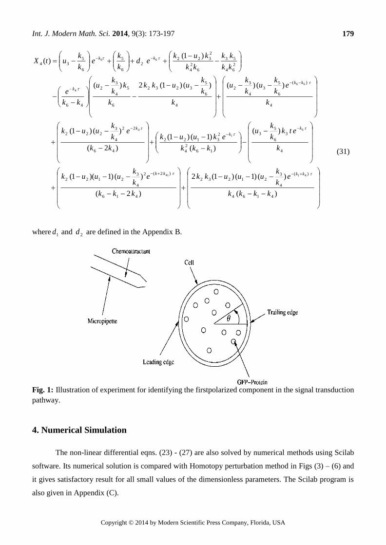
Fig. 1: Illustration of experiment for identifying the firstpolarized component in the signal transduction
pathway.
4. Numerical Simulation
The non-linear differential eqns. (23) - (27) are also solved by numerical methods using Scilab
software. Its numerical solution is compared with Homotopy perturbation method in Figs (3) – (6) and
it gives satisfactory result for all small values of the dimensionless parameters. The Scilab program is
also given in Appendix (C).

Int. J. Modern Math. Sci. 2014, 9(3): 173-197
Copyright © 2014 by Modern Scientific Press Company, Florida, USA
180
Fig. 2: The phosphoinositide cycle (a) and the model scheme (b). In the model scheme, R10 denotes
active receptors; P, I, and Ps denote the pools of membrane phosphoinositicides, cytosolic inosilol and
its phosphates, and phosphoinositicides in the endoplasmic reticulum, respectively.
5. Results and Discussions
Eqns.(28-31) are the new approximate analytical expressions for the ligand –bound sensitive
receptors, membrane phosphoinositicides, stored phosphoinositicides and cytosolic inosilol
phosphates. Figs 3,4 shows the evolution of the solutions when the chemoattractant concentration is
increased from 1000to5.0 . The dimensionless concentration of ligand-bound sensitive
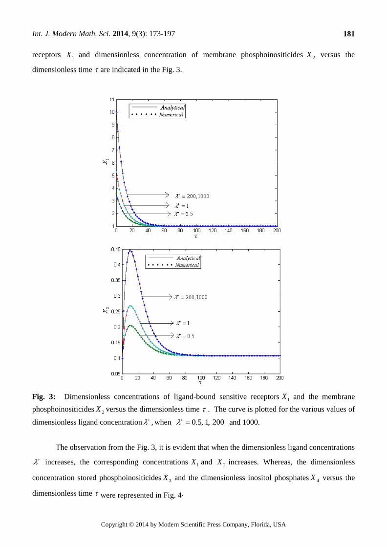
Int. J. Modern Math. Sci. 2014, 9(3): 173-197
Copyright © 2014 by Modern Scientific Press Company, Florida, USA
181
receptors 1X and dimensionless concentration of membrane phosphoinositicides 2X versus the
dimensionless time are indicated in the Fig. 3.
Fig. 3: Dimensionless concentrations of ligand-bound sensitive receptors 1X and the membrane
phosphoinositicides 2X versus the dimensionless time . The curve is plotted for the various values of
dimensionless ligand concentration , when 200,1,5.0 1000.and
The observation from the Fig. 3, it is evident that when the dimensionless ligand concentrations
increases, the corresponding concentrations 1X and 2X increases. Whereas, the dimensionless
concentration stored phosphoinositicides 3X and the dimensionless inositol phosphates 4X versus the
dimensionless time were represented in Fig. 4.

Int. J. Modern Math. Sci. 2014, 9(3): 173-197
Copyright © 2014 by Modern Scientific Press Company, Florida, USA
182
Fig. 4: Dimensionless concentration stored phosphoinositicides 3X and the cytosolic inosilol
phosphates 4X versus the dimensionless time . The curve is plotted for the various values of
dimensionless ligand concentration , when 1000.and200,1,5.0
From the Fig. 4, it is inferred that, when the dimensionless ligand concentration increases,
there was a correspond decrease in the concentration of 3X, and the concentrations of 4X increases
respectively. The ligand bound receptors concentration and membrane phosphoinositicides
concentration is plotted in Fig.5 is a particular case when 2001 and .

Int. J. Modern Math. Sci. 2014, 9(3): 173-197
Copyright © 2014 by Modern Scientific Press Company, Florida, USA
183
Fig. 5: Dimensionless concentrations of ligand-bound sensitive receptors 1X and the membrane
phosphoinositicides 2X versus the dimensionless time . The curve is plotted for the various values of
dimensionless ligand concentration , when 200.and1
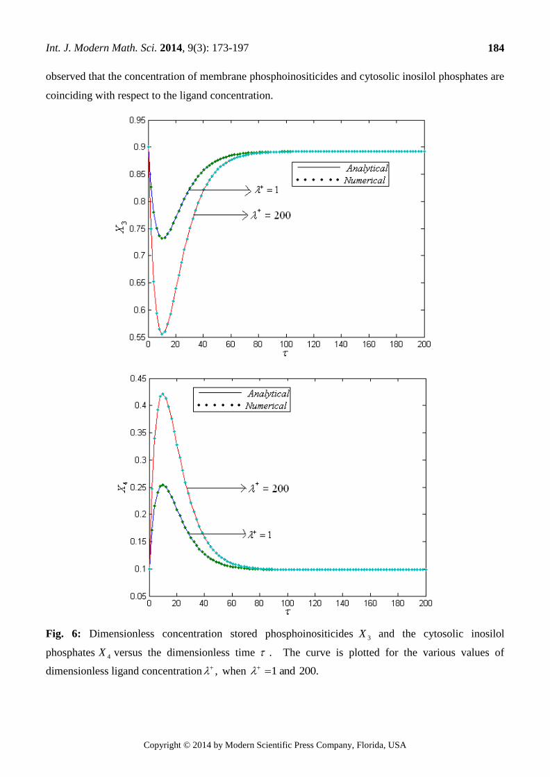
In Fig.6 the concentrations of stored phosphoinositicides and concentrations of cytosolic
inosilol phosphates are varying according to the Ligand concentration. From Fig.7and Fig.8 it is
Int. J. Modern Math. Sci. 2014, 9(3): 173-197
Copyright © 2014 by Modern Scientific Press Company, Florida, USA
184
observed that the concentration of membrane phosphoinositicides and cytosolic inosilol phosphates are
coinciding with respect to the ligand concentration.
Fig. 6: Dimensionless concentration stored phosphoinositicides 3X and the cytosolic inosilol
phosphates 4X versus the dimensionless time . The curve is plotted for the various values of
dimensionless ligand concentration , when 200.and1

Int. J. Modern Math. Sci. 2014, 9(3): 173-197
Copyright © 2014 by Modern Scientific Press Company, Florida, USA
185
Fig. 7: Dimensionless concentrations of ligand-bound sensitive receptors 1X , the membrane
phosphoinositicides 2X , the stored phosphoinositicides 3X and the cytosolicinosilol
phosphates 4X versus the dimensionless time . The curve is plotted for the various values of
dimensionless ligand concentration , when 1.and5.0

Int. J. Modern Math. Sci. 2014, 9(3): 173-197
Copyright © 2014 by Modern Scientific Press Company, Florida, USA
186
Fig. 8: Dimensionless concentrations of ligand-bound sensitive receptors 1X , the
phosphoinositides 2X , the stored phosphoinositicides 3X and the inositol phosphates 4X versus the
dimensionless time . The curve is plotted for the various values of dimensionless ligand
concentration , when 1000.and200

Int. J. Modern Math. Sci. 2014, 9(3): 173-197
Copyright © 2014 by Modern Scientific Press Company, Florida, USA
187
6. Conclusions
It has been observed and concluded that, a reaction-diffusion model based on the kinetics of the
phosphoinositicides cycle captures and explains many of the phosphoinositicides dynamics associated
with directional sensing in cell migration. The analytical expressions of the dimensionless
concentrations of ligand-bound sensitive receptors, membrane phosphoinositicides, stored
phosphoinositicides in endoplasmic reticulum and inosilol phosphates for all the small values of the
corresponding dimensionless parameters. The analytical results are compared to the numerical
simulations. The HPM is an extremely simple compared to other method and it is also a promising
method to solve other non-linear equations. This method can be easily extended to find the solution of
all other non-linear equations.
Acknowledgement
The authors are thankful to Shri. S. Natanagopal, Secretary, Madura College Board, Madurai
and Dr. R. Murali, The Principal for their constant encouragement.
References
[1] JanesS. Tjia and Prabhas V. Moghe, Cell Migration on Cell-Internalizable Ligand Microdepots:
A Phenomenological Model, Annals of Biomedical Engineering, 30(2002):851–866.
[2] Samer J. Nuwayhid, Martha Vega, Paul D. Walden, Marie E. Monaco1,Regulation of de novo
phosphatidylinositol synthesisThe WRP component of the WAVE-1complex attenuates Rac-
mediated signaling, Journal of lipid research, 47 (2006): 1449-1456.
[3] Scott H. Soderling, Kathleen L. Binns, Gary A. Wayman, Stephen M. Davee, Siew Hwa Ong,
Tony Pawson, John D. ScottThe WRP component of the WAVE-1complex attenuates Rac-
mediated signaling, Nature cell Biology,4 (2003): 970-975.
[4] Nathan A. Sallee, Brian J. Yeh, and Wendell A. Lim, Engineering Modular ProteinInteraction
Switches bySequence Overlap, Biophysical Journal, 86 (2004): 589–598.
[5] Jason M. Haugh and Ian C. Schneider, Spatial Analysis of 39 Phosphoinositide Signaling in
Living Fibroblasts: I. Uniform Stimulation Model and Bounds on Dimensionless Groups,Bio
Physical Journal, 86 (2004): 589-598.
[6] Atulnarang, K. K. Subramanian,and D. A. Lauffenburger, A Mathematical Model for
Chemoattractant Gradient Sensing Based on Receptor-Regulated Membrane
PhospholipidSignaling Dynamics, Annals of Biomedical Engineering, 29 (2001): 677-691.

Int. J. Modern Math. Sci. 2014, 9(3): 173-197
Copyright © 2014 by Modern Scientific Press Company, Florida, USA
188
[7] Krishnan Radhakrishnan, A´da´mHala´sz, Dion Vlachos, Jeremy S Edwards, Quantitative
understanding of cell signaling: the importance ofmembrane organization, Current Opinion in
Biotechnology, 21(2010):677–682.
[8] R.Skupsky, W. Losert, R.J. Nossal, Distinguishing Modes of Eukaryotic gradient sensing,
Biophysical Journal, 89(2005): 2806-2823.
[9] S. K Hughes-Alford, D. A Lauffenburger, Quantitative analysis of gradient sensing: towards
building predictive models of chemotaxis in cancer, current opinion in cell Biology, 24(2012):
284-291.
[10] N. Masaki, K. Fujimoto, M. Honda-Kitahara, E. Hada and S. Sawai, Robustness of Self-
Organizing Chemoattractant Field Arising from Precise Pulse Induction of its Breakdown
Enzyme: A Single-Cell Level Analysis of PDE Expression in Dictyostelium, Biophysical
Journal, 104(2013): 1191-1202.
[11] Q.K. Ghori, M. Ahmed, and A. M. Siddiqui, Application of Homotopy perturbation method to
squeezing flow of a Newtonian fluid, Int. J. Nonlinear Sci. Numer. Simulat, 8(2007): 179-184.
[12] T. Ozis, and A. Yildirim, A Comparative study of He’s Homotopy perturbation method for
determining frequency-amplitude relation of a nonlinear oscillator with discontinuities,Int. J.
Nonlinear Sci. Numer. Simulat, 8 (2007): 243-248.
[13] S. J. Li, and Y. X. Liu, An Improved approach to nonlinear dynamical systemidentification
using PID neural networks, Int. J. Nonlinear Sci. Numer. Simulat, 7 (2006): 177-182.
[14] M. M. Mousa, S.F. Ragab, and Z. Nturforsch, Application of the Homotopy perturbationmethod
to linear and nonlinear Schrödinger equations,. Zeitschrift für Naturforschung, 63(2008): 140-
144.
[15] J.H. He, Homotopy perturbation technique, Comp Meth. Appl. Mech. Eng, 178(1999): 257-262.
[16] J. H. He, Homotopy perturbation method: a new nonlinear analytical technique, Appl.Math.
Comput, 135(2003): 73-79.
[17] J. H. He., A simple perturbation approach to Blasius equation, Appl. Math. Comput, 140(2003):
217-222.
[18] P.D. Ariel, Alternative approaches to construction of Homotopy perturbation Algorithms, Non-
linear. Sci. Letts. A., 1(2010): 43-52.
[19] V. Ananthaswamy, SP. Ganesan and L. Rajendran, Approximated analytical solution ofnon-
linear boundary value problem in steady state flow of a liquid film: Homotopy perturbation
method, International Journal of Applied Sciences and Engineering Research(IJASER), 5
(2)(2013):569- 577.

Int. J. Modern Math. Sci. 2014, 9(3): 173-197
Copyright © 2014 by Modern Scientific Press Company, Florida, USA
189
[20] A. Meena and L Rajendran, Mathematical modeling of amperometric and potentiometric
biosensors and system of non-linear equations –Homotopy perturbation approach, J. Electroanal
Chem, 644(2010): 50-59.
[21] S. Anitha, A. Subbiah, S. Subramaniam and L. Rajendran, Analytical solution of amperometric
enzymatic reactions based on Homotopy perturbation method, Electrochimica Acta, 56(2011):
3345-3352.
[22] V. Ananthaswamy and L. Rajendran, Analytical solution of two-point non-linear boundary value
problems in a porous catalyst particles, International Journal of Mathematical Archive, 3
(3)(2012): 810-821.
[23] V. Ananthaswamy and L. Rajendran, Analytical solutions of some two-point non-linear elliptic
boundary value problems, Applied Mathematics, 3(2012): 1044-1058.
[24] V. Ananthaswamy and L. Rajendran, Analytical solution of non-isothermal diffusion-reaction
processes and effectiveness factors, ISRN Physical Chemistry, Article ID 487240, 2012: 1-14.

Int. J. Modern Math. Sci. 2014, 9(3): 173-197
Copyright © 2014 by Modern Scientific Press Company, Florida, USA
190
Appendix A
Basic concept of Homotopy perturbation method [11-24]
To explain this method, let us consider the following function:
r ,0)()( rfuDo (A. 1)
with the boundary conditions of
r ,0) ,(
n
uuBo (A. 2)
where oD is a general differential operator, oB is a boundary operator, )(rf is a known analytical
function and is the boundary of the domain . In general, the operator oD can be divided into a
linear part L and a non-linear part N . Eq. (A.1) can therefore be written as
0)()()( rfuNuL (A. 3)
By the Homotopy technique, we construct a Homotopy ]1,0[:),( prv that satisfies
.0)]()([)]()()[1(),( 0 rfvDpuLvLppvH o (A. 4)
.0)]()([)()()(),( 00 rfvNpupLuLvLpvH (A. 5)
wherep [0, 1] is an embedding parameter, and 0u is an initial approximation of Eq. (A. 1) that
satisfies the boundary conditions. From Eq. (A.4) and Eq. (A.5), we have
0)()()0,( 0 uLvLvH (A. 6)
0)()()1,( rfvDvH o (A. 7)
When p=0, Eq. (A.4) and Eq. (A.5) become linear equations. When p =1, they become non-linear
equations. The process of changing p from zero to unity is that of 0)()( 0 uLvL to 0)()( rfvDo .
We first use the embedding parameter p as a “small parameter” and assume that the solutions of Eq.
(A.4) and Eq. (A.5) can be written as a power series in p :
...2
2
10 vppvvv (A. 8)
Setting 1p results in the approximate solution of Eq. (A.1):
...lim 2101
vvvvup
(A. 9)
This is the basic idea of the HPM.

Int. J. Modern Math. Sci. 2014, 9(3): 173-197
Copyright © 2014 by Modern Scientific Press Company, Florida, USA
191
Appendix B
Solution of the boundary value problem eqns. (23) - (27) using Homotopy perturbation method.
In this Appendix, we indicate how eqns. (28) - (31) are derived in this paper. Solving eqns. (23) and
(27) we get the solution is
1)1( 11 euX (B.1)
To find the solution of the eqns. (24) – (27), we construct the Homotopy as follows:
0)1( 3423
2
212242
3242
kXXXXXkXk
dt
dxpkXk
dt
dXp (B.2)
0)1( 3423
2
212243
3243
kXXXXXkXk
dt
dXpkXk
dt
dXp (B.3)
0)1( 5423
2
212464
5464
kXXXXXkXk
dt
dXpkXk
dt
dXp (B.4)
The analytical solutions of (B.2), (B.3) and (B.4) is
..........210 22
2
21202 XpXpXX (B.5)
.........210 32
2
31303 XppXXX (B.6)
.........210 42
2
41404 XppXXX (B.7)
Substituting the eqns. (B.5), (B.6) and (B.7) in (B.2), (B.3) and (B.4) respectively we get
0
.....).....)((
.....)(.....)(
.....)(.....)(
.....)(.....)(
)1(
342
2
414022
2
2120
32
2
3130
2
22
2
212012
22
2
21204
22
2
2120
322
2
21204
22
2
2120
210210
210210
210
210
210
210
kXpXpXXpXpX
XpXpXXpXpXXk
XpXpXkdt
XpXpXd
p
kXpXpXkdt
XpXpXdp
(B.8)
0
.....).....)((
.....)(.....)(
.....)(.....)(
.....)(.....)(
)1(
342
2
414022
2
2120
32
2
3130
2
22
2
212012
22
2
21204
32
2
3130
322
2
21204
32
2
3130
210210
210210
210
210
210
210
kXpXpXXpXpX
XpXpXXpXpXXk
XpXpXkdt
XpXpXd
p
kxpXpXkdt
XpXpXdp
(B.9)

Int. J. Modern Math. Sci. 2014, 9(3): 173-197
Copyright © 2014 by Modern Scientific Press Company, Florida, USA
192
0
.....).....)((
.....)(.....)(
.....)(.....)(
.....)(.....)(
)1(
542
2
414022
2
2120
32
2
3130
2
22
2
212012
42
2
41406
42
2
4140
542
2
41406
42
2
4140
210210
210210
210
210
210
210
kXpXpXXpXpX
XpXpXXpXpXXk
XpXpXkdt
XpXpXd
p
kXpXpXkdt
XpXpXdp
(B.10)
Comparing the coefficients of like powers of p in (B.8), (B.9) and (B.10) we get
0: 3204
200
0 kXk
dt
Xdp (B.11)
0: 3
300 kdt
Xdp (B.12)
0: 5406
400
0 kXk
dt
dXp (B.13)
402030
2
0212214211 : XXXXXkXk
dt
dXp (B.14)
402030
2
0212214
311 : XXXxXkXkdt
dXp (B.15)
402030
2
0212216411 : xxxxxkxk
dt
dxp (B.16)
The initial approximations are as follows
340230220110 )0(and1)0(,)0(,)0( uXuXuXuX (B.17)
,0)0()0()0()0( 4321 iiii XXXX ......3,2,1i (B.18)
Solving the eqns. (B.11) - (B.16) and using the initial conditions (B.17) and (B.18) we obtain the
following results:

Int. J. Modern Math. Sci. 2014, 9(3): 173-197
Copyright © 2014 by Modern Scientific Press Company, Florida, USA
193
(B.19)4
3
4
3220
4
k
ke
k
kuX
k
1
)(
4
321232
6
)(
6
43
4
32
41
)2(2
4
32122
644
3
6
53
1424
23122
4
22
4
3222
4
6
53232
6
52
624
53
34
2322
121
64
6441
6
1
4
44
)()1()1(2
)()(
)(
)()1()1(
)(
)(
)(
)1()1()()1(
)()1(2)1(
k
ek
kuuukk
k
ek
ku
k
ku
kk
ek
kuuuk
kkk
ekk
ku
kkk
ekuuk
k
ek
kuuk
k
k
kuukk
k
kvet
kk
kk
k
kukedX
kk
kkkk
k
k
k
kk
(B.20)
Where
1
4
321232
6
6
43
4
32
41
2
4
32122
644
3
6
53
1424
23122
4
2
4
3222
34
2322
624
531
)()1()1(2
)()(
)(
)()1()1(
)(
)(
)(
)1()1()()1(
)1(
k
k
kuuukk
k
k
ku
k
ku
kk
k
kuuuk
kkk
kk
ku
kkk
kuuk
k
k
kuuk
k
kuk
kk
kkd
(B.21)
Since ,032 d
dX
d
dX we get
23 1 XX
(B.22)

Int. J. Modern Math. Sci. 2014, 9(3): 173-197
Copyright © 2014 by Modern Scientific Press Company, Florida, USA
194
(B.23)6
5
6
5340
6
k
ke
k
kuX
k
(B.24)
)()(
)(
)()1()1(2
)2(
)()1)(1(
)(
)(
)1()1(
)2(
)()1(
)()1(2)()1(
4
)(
6
53
4
32
4164
)(
4
321232
416
)2(2
4
32122
4
3
6
53
1624
23122
46
22
4
3222
4
6
53232
6
5
4
32
46264
53
624
2322
241
6641
14
6
1
4
46
k
ek
ku
k
ku
kkkk
ek
kuuukk
kkk
ek
kuuuk
k
ekk
ku
kkk
ekuuk
kk
ek
kuuk
k
k
kuukk
k
kk
ku
kk
e
kk
kk
kk
kukedX
kkkk
kk
k
k
k
kk
where
4
6
53
4
32
4164
4
321232
416
2
4
32122
4
3
6
53
1624
23122
46
2
4
3222
4
6
53232
6
5
4
32
46624
2322
264
532
)()(
)(
)()1()1(2
)2(
)()1)(1(
)(
)(
)1()1(
)2(
)()1(
)()1(2)(1)1(
6
k
k
ku
k
ku
kkkk
k
kuuukk
kkk
k
kuuuk
k
etkk
ku
kkk
kuuk
kk
k
kuuk
k
k
kuukk
k
kk
ku
kkkk
kuk
kk
kkd
tk
(B.25)
According to the HPM, we can conclude that
)(lim10 21202
12 XXtXX
p
(B.26)

Int. J. Modern Math. Sci. 2014, 9(3): 173-197
Copyright © 2014 by Modern Scientific Press Company, Florida, USA
195
1 23 XX (B.27)
)(lim10 41404
14 XXtXX
p
(B.28)
After putting the eqns. (B.19) and (B.20) into an eqn. (B.26) and (B.23) and (B.24) into an eqn.
(B.28), we obtain the solutions in the text eqns. (29) and (31).
Appendix C
Scilab program to find the solutions of the Equations (23)-(27)
function
options= odeset('RelTol',1e-6,'Stats','on');
%initial conditions
x0 = [10.08174387; .1; .9; .1];
tspan = [0,200];
tic
[t,x] = ode45(@TestFunction,tspan,x0,options);
toc
figure
hold on
%plot(t, x(:,1))
%plot(t, x(:,2))
plot(t, x(:,3))
%plot(t, x(:,4))
legend('x','y','z')
ylabel('x')
xlabel('t')
return
function [dx_dt]= TestFunction(t,x)
k1=.09523809524;k2=1.1;k3=.01;k4=.1;k5=.01;k6=.11;
dx_dt(1)=k1*(1-x(1));
dx_dt(2)=k2*x(1)*x(2)^2*x(3)-x(2)*x(4)+k3-k4*x(2);
dx_dt(3)=-(k2*x(1)*x(2)^2*x(3)-x(2)*x(4)+k3-k4*x(2));
dx_dt(4)=k2*x(1)*x(2)^2*x(3)-x(2)*x(4)+k5-k6*x(4);
dx_dt = dx_dt';
return

Int. J. Modern Math. Sci. 2014, 9(3): 173-197
Copyright © 2014 by Modern Scientific Press Company, Florida, USA
196
Appendix D
Nomenclature
Symbols Meaning
ija Rate constants for association of aE or dE with ijR
la Rate constants for association of ijR with L
ic Basal synthesis rate of synthesis of inosital phosphates
c Circumference of the cell
iD Lateral diffusivity of inosital phosphates
pD Lateral diffusivity of phoshoinositides in plasma membrane
spD Lateral diffusivity of phoshoinositides in endoplasmic
reticulum
rD Lateral diffusivity of receptors
tae , Total concentration of activating (dephosphorylating ) enzyme
de Concentration of deactivating (phosphorylating ) enzyme
i Concentration of inositol phosphates
fk Rate constant for receptor-mediated phoshoinositide formation
ik Rate constant for basal degradation of inositolphosphates
pk Rate constant for basal degradation of phosphoinositides
rk Rate constant for removal of phosphoinositides
ijk Rate constants for sensitization/ desensitization
ijK Dissociation constants for binding of aE or dE to ijR
lK Dissociation constant for ligand binding
l Concentration of ligand
p Concentration of membrane phosphoinositides
sp Concentration of phosphoinositides on endoplasmic reticulum
lp Average concentration of phosphoinositides in the cell
ijr Concentration of receptors with i ligand-bound and j
phosphorylated sites
*ij
r Concentration of complexes between aE or dE and ijR
fpr , Rate of formation of membrane phosphoinositides
rpr , Rate of removal of membrane phosphoinositides
dpr , Degradation rate of membrane phosphoinositides
dir , Degradation rate of inositol phosphates
R Radius of the cell
s Membrane length per unit cell area

Int. J. Modern Math. Sci. 2014, 9(3): 173-197
Copyright © 2014 by Modern Scientific Press Company, Florida, USA
197
p Dimensionless rate of basal synthesis of phosphoinositides
i Dimensionless rate of basal synthesis of inositol phosphates
i Dimensionless angular diffusivity of inositol phosphates
p Dimensionless angular diffusivity of phosphoinositides in
plasma membrane
sp Dimensionless angular diffusivity of phosphoinositides in
endoplasmic reticulum
r Dimensionless angular diffusivity of receptors
Ι Dimensionless concentration of inositol phosphates
ta, Dimensionless concentration of activating enzyme
d Dimensionless concentration of deactivating enzyme
f Dimensionless rate constant for formation of
phosphoinositides
i Dimensionless rate constant for degradation of inositol
phosphates
p Dimensionless rate constant for degradation of
phosphoinositides
Dimensionless ligand concentration
Dimensionless concentration of phosphoinositides
s Dimensionless concentration stored phosphoinositicides
10 Dimensionless concentration of ligand-bound sensitive
receptors
Relative gradient of chemoattractant
Dimensionless time
Angular coordinate scaled between 0 and 1
Copyright © 2022 FDOKUMEN


![Interfacial interactions between poly[L-lysine]-based branched polypeptides and phospholipid model membranes](https://static.fdokumen.com/doc/165x107/633df5f7df741406dc0b4c83/interfacial-interactions-between-polyl-lysine-based-branched-polypeptides-and.jpg)