Applications of Multinomial Dose-Response Models in Developmental Toxicity Risk Assessment

Risk Analysis, Vol. 14, No. 4, 1994

Applications of Multinomial Dose-Response Models in Developmental Toxicity Risk Assessment

D. Krewski'f and Y. Zhu'

Received February 2, 1994

Reproductive and developmental anomalies induced by toxic chemicals may be identified using laboratory experiments with small mammalian species such as rats, mice, and rabbits. In this paper, dose-response models for correlated multinomial data arising in studies of developmental toxicity are discussed. These models provide a joint characterization of dose-response relationships for both embryolethality and teratogenicity. Generalized estimating equations are used for model fitting, incorporating overdispersion relative to the multinomial variation due to correlation among littermates. The fitted dose-response models are used to estimate benchmark doses in a series of experiments conducted by the U.S. National Toxicology Program. Joint analysis of prenatal death and fetal malformation using an extended Dirichlet-trinomial covariance function to characterize overdispersion appears to have statistical and computational advantages over separate analysis of these two end points. Benchmark doses based on overall toxicity are below the minimum of those for prenatal death and fetal malformation and may, thus, be preferred for risk assessment purposes.

KEY WORDS: Benchmark dose; correlated multinomial response; dose-response; developmental toxicity; estimating equations; embryolethality; teratogenicity.

1. INTRODUCTION

An important component of developmental toxicity risk assessment is modeling of the dose-response relationship induced by a test agent. However, dose-response models for developmental toxicity data may differ from those used to describe other toxicological data in several respects.

First, multivariate binary responses of animals within the same litter may demonstrate some degree of extramultinomial variation as a consequence of intralitter correlation. Such litter effects are due to the fact that observations on the same mother (including embryolethality and malformations among live offspring) tend to be more alike than observations from different mothers.

Second, the number of animals per litter is a random variable that may be affected by the test agent. And third, since developmental toxicity studies provide direct information on both embryolethality and fetal malformations, a joint analysis of these two related endpoints is desirable.

Dose-response models for developmental toxicity data can be used to estimate benchmark doses (BMDs) for risk assessment.('-') The BMD is defined as the dose inducing a specified increase in risk such as 5% within the experimentally measurable response range and provides a measure of potency of developmental toxicants. The BMD has certain advantages in comparison with traditional methods used in risk assessment based on the no-observed adverse-effect level (NOAEL) and lowest- observed adverse-effect level ((LOAEL). Specifically, ~- the BMD provides an indication of the potential risk associated with exposures near the NOAEL, taking into account both the experimental error and the shape of the dose-response curve. The U.S. Environmental Protection

I Health Protection Branch, Health and Welfare Canada, Ottawa, On- tano, Canada K1A OL2. Department of Mathematics and Statistics, Carleton University, Ot- tawa, Ontario, Canada KlS SB6.

613 0272-4332/94DBM)-o613S~.WlO 1994 Society for Risk Analysis

614 Krewski and Zhu

Agencycs) has recently recommended the BMDs as an alternative or adjunct to the methods based on the NOAEL and LOAEL.

The purpose of this paper is to discuss conditional simultaneous dose-response modeling for correlated trinomial count data (i.e., embryolethality and fetal malformations) and to use these models to estimate BMDs for developmental toxicants. Generalized estimating equations (GEES) are used for model fitting in conjunction with an extended Dirichlet-multinomial covariance function, hence allowing for a flexible treatment of overdispersion. BMDs obtained from joint (trinomial) dose-response models are also compared with those obtained from separate (binomial) dose-response models. Our experience in estimating BMDs for a series of developmental toxicants tested under the U.S. National Toxicology Program is also reported.

Statistical model assumptions are discussed in Sec- tion 2. In Section 2.1, a hierarchical probability structure which embraces existing methods is introduced to provided a probabilistic basis for joint and separate inference on endpoints arising in developmental toxicity studies. The extended Dirichlet-trinomial covariance function used to characterize the correlation among littermates is specified in Section 2.2. Weibull dose-response models are described in Section 2.3. Marginal models for implant number and litter size are outlined in Section 2.4. In Section 3, generalized estimating equations are presented for both joint and separate modeling. The estimation of BMDs is described in Section 4. In Section 5, these methods are applied to a series of experiments conducted under the U.S. National Toxicolog- ical Program. Our conclusions are presented in Section 6.

2. STATISTICAL MODELS

2.1. Multinomial Outcomes

In developmental toxicity studies, female animals are exposed to one of several doses of the test agent, and the toxic effects on each fetus examined. Data from such experiments can be conveniently summarized in the form of multinomial counts. Observations for each female typically includes the total number of implants m, the total number of prenatal deaths r (including both resorbed implants and dead pups), the number of live offspring s, and the number of malformed live offspring y . Given the total number of implants m, the response (y,r,s - y ) is a trinomial random variate. Modeling (y,r,s

- y ) is equivalent to modeling (y,r) or (y,s) due to the constraint s = m - r. Further mutually exclusive clas- sification of the three categories may occur (such as the disaggregation of resorptions and stillbirths), thereby yielding multinomial responses of higher dimension. The methods discussed below can be easily generalized to the case of higher-dimensional multinomial response data.

The incidences of fetal malformation yls and prenatal death rlm are of particular interest, measuring teratogenicity and embryolethality, respectively. Although other parameters such as fetal weight are also of impor- tantcet6) our focus in this paper is on simultaneous modeling of the dose-response relationships and subsequent estimation of BMDs for fetal malformation and prenatal death based on the trinomial observations (y,r,s - y). Following Fleiss, (’1 we use the terms “incidence,” “rate,” and “probability” interchangeably throughout this article.

The joint probability P(y,r,m) or P(y,s,m) of ob- serving m implants, among which there are s live fetuses, y malformed live fetuses, and r prenatal deaths, may be factored as

PCy,r,m) = P@,r I m)P(m) where the probability P(m) represents the marginal distribution of the implant number rn. Since the test agent is normally administered to the mother after mating, the random variable m is an ancillary statistic containing no information about the dose-response relationship for developmental toxicity. Therefore, joint inference for yls and rlm is naturally based on the conditional distribution P(y,r I m), which is further factored as

P(yJ I m) = pot I ~,m)P(r I m) (1) Here the conditional probability P(y I s,m) characterizes the fetal malformation rate, conditional on the number of implants m and the number of live births s; the probability P(r I m) reflects the prenatal death rate. Equation (1) postulates a conditional litter-specific joint model for embryolethality and teratogenicity and forms the basis for statistical inference in this article.

Chen er U L ( ~ ) suggested a Dirichlet-trinomial distribution for P(y, r I m). Although a likelihood-ratio test for treatment effects was proposed, formal dose-response modeling was not undertaken. Under the Diri- chlet-trinomial distribution, the factorization in (1) yields beta-binomial distributions for P o I s, m) and P(r I m). The latter component is the result of collapsing the malformed (y) and normal live births (s - y ) into one cat- egory, and the former is the result of further conditioning on the collapsed total s. In general, Dirichlet-multino-

Multinomial Dose-Response Models for Developmental Toxicity 615

mial distributions of arbitrary dimension can be factored in a similar fashion through collapsing and conditioning. Under the factorization in (l), PO, I s, m) may be used as the basis for separate inference on y/s. However, separate inference suffers from information loss since the two submodels both contain information on the dose- response relationship for developmental toxicity.

Specification of a fully parametric model such as the Dirichlet-trinomial distribution can be avoided using non-likelihood-based methods for statistical inference. Recently, Ryan@) considered joint dose-response modeling based on PO,,r I m) using quasi-likelihood methods. The doseresponse models were marginal (i.e., independent of m), and a simplified characterization of overdispersion was used for computational convenience. In contrast, we use joint Weibull doseresponse models conditional on m and use GEEs for model fitting incorporating an extended Dirichlet-trinomial covariance function specific to each dose group.

Rai and Van Ry~in(~) employed the population-average (marginal) model

PO,,s) = s.PO,,s,m)n(m) = PO, I s)P(s) (2) as a basis for inference. By using a binomial distribution for PO, I s), however, they assumed that littermates re- spond independently conditional on s. Further, by as- suming a Poisson distribution for p ( ~ ) , it is not possible to accommodate overdispersion or underdispersion of litter size s relative to the Poisson distribution reported by other investigators.(loJ1)

Although we focus primarily on joint analyses of prenatal death and fetal malformation, separate analyses on each of these endpoints have been conducted previ- ously. For example, a number of in~estigatord~”’~) have used a beta-binomial distribution for PO, I s) in analyzing malformation rate yls. Other extended binomial distributions(16J‘) have also been suggested for PO, I s). Since s is not an ancillary statistic, conditioning on s results in loss of information. As discussed later, separate inference may be more sensitive to extreme observations than joint inference. Nonetheless, we present some results on separate modeling of the malformation rate yls, prenatal death rate r/m, and overall toxicity 0, + r)/m based on PO, I s), P(r I m), and PO, + r I m), respectively, for purposes of comparison with joint modeling.

2.2. Overdispersion

Developmental toxicity data often demonstrate positive intralitter correlation, resulting in overdispersion

relative to multinomial variation. We propose the following mean and covariance functions to characterize overdispersion associated with PO,,r I m). Letting z = ( y,r)r, we assume

and

cov(z I m) = m(l+(m-1)+)(1-?r2) x

) (4) ( -?r1lrz =2

=1[1-=1(1-~2)1 -=1nz

where E ( y I s) = sr1, and + represents the intralitter correlation. When + > 0, the covariance function in (4) is that of Dirichlet-trinomial distribution. In the limiting case + = 0, it reduces to that of the trinomial distribution. When

Pi * i = 1,2,3; m22 m-l-p,’

with = 1 - p, - k, the covariance function corresponds to that of an extended Dirichlet-trinomial distribution.(lO) Here, we permit -(m -l)-l < + < 0 to allow for underdispersion. Although intralitter correlation could be modeled as a function of dose$1am) we postu- late a unique value of + for each dose group to allow for possible dose dependency. In addition to allowing for underdispersion, the extended Dirichlet-trinomial covariance function in (4) is more flexible than that used by Ryan,(2) which involves a single constant across dose groups and dams to inflate the trinomial covariance. However, because of the upper bound + 5 1, it may not be able to describe extremely large overdispersion using

Since EO,/sIs,m) = ?r, and E(r/rnlm) = T ~ , we use the parameterization (al, m2, 4) in joint dose- response modeling. Notice that under the factorization in (l), the variance of the conditional distribution Pot I s,m) is

VarO, I s,m) = s~r~(l-~r,)[l+(~-l)p]

where the intralitter correlation coefficient among live fetuses p 2 -(s - l)-l satisfies the relationship + = p(1 - TJ(~ -paz)-l. Therefore, separate modeling of y /s based on PO, I s,m) involves the natural parametri- zation (n,,p). The extended beta-binomial variance for P(r I m) and PO, + r I m) can be easily obtained as special cases of (4). Separate modeling of r/m and O, + r)/m thus involves the parametrizations ( ~ ~ 4 ) and (1 -(1 - q)(l - ITJ,+), respectively.

(4).

616 Krewski and Zhu

2.3. Dose-Response Models

The main objective of this paper is to model jointly the dependency of T, and T, on dose d. In this regard, consider the Weibull dose-response models

rl(d I m) = 1 - exp[-(a,+c,rn+b,dri)] (5)

and

~ , ( d I m) = 1 - exp[-(a,+c,m+b,&)] (6) for fetal malformation and prenatal death. This implies a model for overall toxicity 0, + r)/m given by

n3(d I m) = 1 - (1 - Tl(d I m))(l - T*(d I 4 ) (7)

Kodell et al.(') also used Weibull models to describe the dose-response relationship for PO, I s) and included a threshold dose below which developmental toxicity is assumed not to occur. Such a threshold dose is not employed here since the threshold, being outside the ob- servable response range, will not be well determined and will have little impact on predictions of risk within the experimentally measurable response range. An interaction term based on the product of dose d and the implant number m may, however, be useful in achieving a better model fit in practice.

The constraints a, + cpz 2 0 and b, 2 0 are required to ensure 0 s Ti s 1. Although m > 0 in practice, the models theoretically permit m = 0, leading to the further constraints a, 2 0. Notice that 1 - exp[-(a, + ciA)] is the population-average probability of an anomaly occur- ing spontaneously in the absence of exposure to the test agent, where A denotes the average number of implants per dam. The dependence of models (5) and (6) on m is in line with the conditional model in (1) and accounts for variability across litters. For model fitting purposes, the two sets of parameters 0, = (a, b , c,, yi)* (i = 1,2) involved in r , and n2, respectively, are considered to be functionally independent.

The Weibull parameter y, determines the shape of the dose-response curve. For y, < 1 the curve is concave; for y, > 1 the curve is convex when d < [(l - r;l)b;l]wi and concave when d > [(l - No- tice the inflection point is a strictly increasing function of yi and, with dose scaled to lie in the range [0,1], approaches 1 as yi --t m. These properties suggest that the Weibull model may not be suitable for use with certain data. Although models of a form other than that of (5) and (6) may be useful in such cases, the Weibull model is relatively flexible and is used in the applications in Section 5.

In separate modeling, dose-response models can be specified as in (5) and (6) in conjunction with a variance

function corresponding to PO, I s,m), P(r I m), or PO, + r I m). However, a special case arises when modeling yls based on PCy I s) instead of PCy I s,m). Substi- tuting s for m in (5), we obtain a simplified version

n;(d I s) = 1 - exp[-(a,+c,s+b,rtvi)] (8)

of the model proposed by Kodell et ul.(l) without a threshold or interaction term between litter size and dose. The difference between ~ ; ( d I s) and r , (d I m) is that the former is a marginal model with respect to m, whereas the latter is conditional. An advantage of the latter model is that ~ , ( d I m) can be used in conjunction with r2(d I m) to recover the marginal probability p,(d I m) = ~ , ( d I m)[l - r2(d I m)] of a malformation, given the implant number m and the probability of either fetal death or malformation in (7). In contrast, ~ ; ( d I s) cannot be interpreted in a conditional fashion given m.

In the applications in Section 5, the term binomial model refers to separating modeling of rlm, of 0, + r)/m, and particularly of yls using T; in (8). The term trinomial model refers to the joint models r,, T ~ , and r3 in (9, (6), and (7).

2.4. Litter Size and Implant Number

Although specification of P(s) reflects the marginal distribution of prenatal death, a conditional model for P(r I rn) is more relevant in characterizing embryolethality due to the constraint r + s = m. Our results on marginal modeling of s conducted in Section 5 support this preference. A reasonable marginal model for P(m), on the other hand, will cast additional light on the population-average dose effect. For instance, replacing m by its marginal mean X = E(m) in n,(d I m) and ~ , ( d I rn) gives an approximation to the population-average mean response.

The same modeling techniques can be applied to both litter size s and implant number m. To account for possible overdispersion or underdispersion in s relative to Poisson variation, we assume an extended negative- binomial variance function

VX(S) = A(1 4- KA) (9)

where A = E(s), and K > 0 or K < 0 characterizes overdispersion or underdispersion, respectively. Note that a positive value of K corresponds to a negative- binomial distribution within the exponential family, whereas a negative value of K implies a distribution outside the exponential family. The dose effect on s may be modeled using link function(9)


3. GENERALIZED ESTIMATING EQUATIONS

Both Williams(1z) and Ryan(*) used quasi-likelihood rather than maximum-likelihood methods for model fitting. Recent developments in the use of generalized estimating equations(21) have stimulated application of these methods to correlated binary regression models.(3.22923) The GEE approach allows for relaxed distri- butional assumptions and is often computationally simpler than maximum likelihood. The GEES are equivalent to quasi-likelihood equations when the corresponding quasi-likelihood exists and to likelihood equations when the underlying distribution is in the natural exponential family. Even when the covariance function is misspecified, GEEs can still yield consistent and asymp- totically normal estimates, although efficiency will de- crease. As such, they are widely applicable in practice. In this section, we briefly describe GEES for fitting the conditional joint dose-response models (5) and (6).

3.1. Joint Estimation

Let ( y ip sip m,) be the counts observed from thejth dam (j = 1 ,..., ni) in the ith dose group (i = 1, ..., t). Also, let + = (+l,..., +,), where +i denotes the intralitter correlation coefficient in the ith dose group. We assume that observations from different dams, which constitute the experimental units, are statistically independent.

Letting V, = C~V(Z,~ I m,) as given in (4), it follows that the contribution of each experimental unit to the joint GEEs for OT = (Of, 82 with 9 fixed is

where D = 8p/8OT. The GEEs for 8, and 8, are then given by

and

respectively.

To estimate the correlation parameters +i ( i = 1, ..., t), we use the moment equations

based on the fact that

EeZ, = E((~,-p~)'Vi'(z,-p,)) = 2

Here, n = En,, p is the dimension of 8, and the correc- tion factor (1 - p / h ) is used to adjust for the simultaneous estimation of 8. Since the equations in (11) and (12) do not involve 8, and 8,, respectively, the estimates 61, 6,, and 4 are obtained by iteratively solving Eqs. (ll), (12) and (13) until convergence.

The asymptotic normality of these parameter estimates as each ni + 00 follows from a slight modification of the argument used by Moore.(24) The asymptotic covariance matrix for iT = (@, 69 is given by

1 ni -1

Cov(8) = (z r-lj-1 z D y i l D i j )

Since Cov (6) is block diagonal, 6, and 6, are asymp- totically independent.

The asymptotic covariance for 4 can be calculated in a similar fashion.(11) In computing the asymptotic covariance in our applications reported in Section 5, Var(6) is replaced by its sample version of z, in the interest of However, the variance of $i

can be approximated by

ni

var(+i) = X i-1 [~-2(1-~/(2n))12/

based on (13) only. Note that the moment estimates 4 are biased under

incorrect specification of the variance function. In this event, variance estimators for the estimates of the dose- response model parameters are inconsistent. Improved methods of estimating these dispersion parameters are under investigation.(")

3.2. Separate Estimation

Since derivation of the estimating equations for binomial models is straightforward, the GEES associated with r/m and 0, + r)/m are omitted. The GEEs for fitting IT;(^ I s) based on PO, I s) are obtained by replacing r1

618 Krewski and Zhu

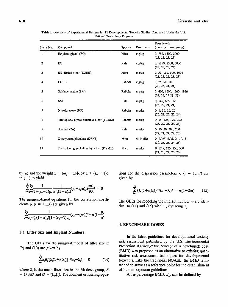
Table I. Overview of Experimental Designs for 11 Developmental Toxicity Studies Conducted Under the U.S. National Toxicology Program

Study No. Compound Dose levels

Species Dose units (darns per dose group)

1

2

3

4

5

6

7

8

9

10

11

Ethylene glycol (EG)

EG

EG diethyl ether (EGDE)

EGDE

Sulfamethezine (SM)

SM

Nitrofurazone (NF)

Triethylene glycol dimethyl ether (TGDM)

Analine (2A)

Diethylhexalphthalate (DEHP)

Diethylene glycol dimethyl ether (DYME)

Mice

Rats

Mice

Rabbits

Rabbits

Rats

Rabbits

Rabbits

Rats

Mice

Mice

0, 750, 1500, 3000 (25, 24, 23, 23)

0,1250,2500,5000 (28, 28, 29, 27)

0, 50, 150,500, 1000 (23, 24, 22, 23, 23)

0, 25, 50, 100 (26, 22, 24, 24)

0, 600, 1200, 1500, 1800 (24, 26, 25 28, 23)

0, 545, 685, 865 (26, 22, 24, 24)

0, 5, 10, 15, 20 (25, 23, 27, 22, 24)

0, 75, 125, 175, 250 (25, 22, 25, 23, 23)

0, 10, 30, 100, 200 (22, 21, 24, 22, 25)

0, 0.025, 0.05, 0.1, 0.15 (30, 26, 26, 24, 25)

0, 62.5, 125, 250, 500 (21, 20, 24, 23, 23)

by IT; and the weight 1 + (mu - l)~$~ by 1 + (sij - l)pi in (11) to yield

The moment-based equations for the correlation coefficients pi (i = l,...,t) are given by

tions for the dispersion parameters K~ (i = l , . . .~ ) are given by

ni

2 {hi( 1 + K~A~)}-~(S~- hi)z = ni(l-2/n) (15) 1’1

The GEEs for modeling the implant number m are iden- tical to (14) and (15) with mu replacing sij.

4. BENCHMARK DOSES

3.3. Litter Size and Implant Numbers

The GEEs for the marginal model of litter size in (9) and (10) are given by

where Si is the mean litter size in the ith dose group, Bi = ahi/agT and 5’ = ({&). The moment estimating equa-

In the latest guidelines for developmental toxicity risk assessment published by the U.S. Environmental Protection Agency,@) the concept of a benchmark dose (BMD) was proposed as an alternative to existing quantitative risk assessment techniques for developmental toxicants. Like the traditional NOAEL, the BMD is intended to serve as a reference point for the establishment of human exposure guidelines.

An a-percentage BMD, d,, can be defined by


1. EG (mice) 2. EG (rats) 3. EGDE (mice) I

6 0 0

0 0

0 0

0 500 1500 2500 0 1000 2000 3000 4000 5000

4. EGDE (rabbits)

Dose

5. SM (rabbits)

I 0 200 400 600 800 1000

6. SM (rats)

0 500 to00 1500

Dose

Fig. 1. Trinomial dose-response models for 11 developmental toxicity studies. (3 Litter-specific response rate; (x) average response rate across titter; (-) fitted Weibull model evaluated at A = E(m).

620 Krewski and Zhu

7. NF (rabbits) 8. TGDM (rabbits) 9. 2A (rats)

- l* zo d 0 iL 0 0 5 10 15 20

0 50 100 150 200 250

Dose

1 50

10. DEHP (mice) 11. DYME (mice)

I

r p - 1- bO

d 0 1

0

00 005 010 015

0 0 ii//i 0 100 200 300 400 500

100 150 200

Dose Fig. 1. Continued.


Table II. Estimates of the Parameters of Trinomial Dose-Response Models Fitted to 11 Developmental Toxicity Studies (Standard Error in Parentheses)

Fetal malformations Prenatal death Correlation

1

2

3

4

5

6

7

8

9

10

11

ob

ob

ob

0.0238 (0.0599) 0.0476 (0.0415) 0.0582 (0.0598) 0.0332 (0.0373)

0.0645 (0.0846) 0.0107 (0.0255)

ob

ob

0.8828 (0.1419) 1.2300 (0.2211) 1.8015 (0.3186) 0.6949 (0.1534) 0.0267 (0.0359) 0.1841 (0.0508) 0.0582 (0.0497) 1.2475 (0.2821) 0.3434 (0.0746) 1.8447 (0.5324) 2.8728 (0.5494)

0.0002 (0.0003) 0.0009 (0.0006) 0.0001 (0.0001) 0.0048 (0.0071) 0.0003 (0.0042) -0.0014 (0.0044) .oooo3

(0.0038) -0.0002 (0.0087) 0.0004 (0.0026) 0.0009 (0.0008) 0.0001 (0.0001)

1.4585 (0.2020) 2.2227 (0.2808) 3.1621 (0.4925) 3.5045 (1.3148) 1.6318 (4.6881) 6.1933 (2.7396) 8.1369

(18.586) 2.5771 (0.5652) 5.4956 (3.1036) 2.6984 (0.4267) 3.5642 (0.3088)

0.1632 (0.0938)

ob

0.1976 (0.0892) 0.1175 (0.0800) 0.2076 (0.0686)

0.1333 (0.0573) 0.0869 (0.0613) 0.1318 (0.0956) 0.1616 (0.0555) 0.1793 (0.0879) 0.1509 (0.0537)

0.1150 (0.0595) 0.1866 (0.0700) 0.3193 (0.0826) 0.2681 (0.0901) 0.2860 (0.0852)

o.oO01 (0.0250) 0.2544 (0.0875) 0.6331 (0.1367) 0.1600 (0.0520) 1.8849 (0.2834) 0.6318 (0.0999)

-0.0037 (0.0066) 0.0039 (0.0010) -0.0092 (0.0066) 0.0021 (0.0087)

(0.0071) - 0.006 1

-0.0067 (0.0040)

(0,0064) 0.0016

-0.0022 (0.0098)

(0.0051) -0.0057 (0.0065)

(0.0037)

-0.0093

-0.0066

1.6232 (1.6059) 3.2977 (2.0754) 2.3189 (1.1 663) 3.4013 (3.5433) 6.1546 (3.0667) 1.7262

(2057.4) 9.9674

(11.787) 3.0837 (0.9806) 2.7503 (2.0573) 3.1926 (0.5337) 3.0454 (0.7759)

0.0164 (0.0400) 0.0838 (0.0737) -0.0325 (0.0392) 0.2012 (0.1179)

(0.0229)

0.0272 (0.0219) 0.1102 (0.0526)

0.0377 (0.0254)

(0.0258)

-0.0093

-0.0061

-0.0278 (0.0107) -0.0417 (0.0134)

0.3379 (0.0890) 0.4324 (0.086 1) 0.2633= (0.1172) 0.6009 (0.2310) 0.1978 (0.0845)

0.2355 (0.1194) 0.2927 (0.1152) 0.3647 (0.1381) 0.2225 (0.1109)

(0.2102) 0.4107

0.2051 (0.0663)

Highest dose scaled to unity. * Set to boundary value of zero.

Excluding boundary value of unity.

= a r(da)-T(O) 1-r(0)

where r(d) represents an appropriate doseresponse model for a particular endpoint. Under the Weibull models used here, we have

where the subscript for the parameters b and X is sup- pressed for simplicity. The asymptotic variance of the estimator, a,, is given by

Var(&J = y- 'd~Cy,C, (16)

where V, is the asymptotic covariance matrix of the estimates (by yy and

C, = (bl, y-'log[-b-'log(l - a)])'

The BMD associated with overall toxicity based on our trinomial model is obtained as the solution to

b,@ + b,@ = -lOg(l - a)

Using a first-order Taylor series approximation to this equation, the asymptotic variance of the estimator 2, of d, is given by

Var(2.J = [blyI@ + b 2 y 2 ~ z - 1 ] - z C ~ z C z (17)

where V, is the asymptotic covariance matrix of the estimates (b,, f,, b2, 93' and

C, = (a1, b,d$logd,, dgz, b,d$logdJT

An estimate of Var (2J is obtained by replacing all unknown parameters by their estimates. The specification and the estimation of the covariance function directly affect the estimates of the covariance matrices V, and V, and, hence, the precision of the estimated BMD.

Krewski and Zhu

0 0

8 0 0

0 0

o o 0

0 0 8

0 0 0 0

8 0 l o o 0 0

0 0 0

8 0

0

0

0

1 I I I I I

1.0 0.2 0.4 0.6 0.8 1 .o Scaled Dose

Fig. 2. Standardized intralitter correlation coefficients as a function of scaled dose (excluding two boundary values of unity).

The rates of fetal malformation, prenatal death, and overall toxicity are shown in Fig. 1 for each litter, along with fitted trinomial dose-response curves. In some cases, a dose-response relationship is not evident for either fetal malformation or prenatal death. For example, the incidence of malformations in studies 5 and 7 and the incidence of prenatal death in study 6 do not seem to be elevated within the range of doses used in these experiments. Examination of the litter-specific response rates within the same group reveals convex (study 4), sigmoidal (malformations in study 1 l), and irregular (study 5 ) dose-response relationships. There can also be large variation in response due to either unknown bio- logical factors or uncontrolled laboratory error. In study 7, for example, the incidence of prenatal death at 15 mg/ kg falls to 0.098 from 0.142 at 10 mg/kg. The pattern of malformation rates in study 1 (increasing markedly from the second to the third dose level, but less so at lower and higher dose levels) is also noteworthy: our discussion in Section 2.3 suggests that the Weibull model may be unable to provide a good description of this type of data.

5. APPLICATIONS 5.2. Model Fitting

5.1. Developmental Toxicity Data

Application of the modeling techniques discussed in the preceding sections is illustrated using data from 11 laboratory experiments conducted under the U.S. Na- tional Toxicology Program (Table I). These developmental toxicity studies typically involve groups of 20- 30 female animals exposed to one of four or five doses, including an unexposed control. In study 1, for example, ethylene glycol (EG) was administered at dose levels of 0, 750, 1500, and 3000 mg/kg, with 25, 24, 23, and 23 animals in each dose group, respectively. These 11 experiments were selected from among 48 experiments provided to us by the National Toxicology Program because the data exhibited a clearly increasing dose-response relationship for fetal malformations or prenatal death and are, thus, candidates for dose-response modeling.

The teratogenic effects observed in these 11 studies included various gross, visceral, and skeletal malformations. In this analysis, we regard any type of malformation as the teratogenic endpoint of interest for simplicity of presentation. Since many teratogens induce multiple malformations, an assessment of any type of malformation is normally done in the analysis of developmental toxicity data, in addition to the analysis of specific malformations.

5.2.1 Dose-Response Modeling

Parameter estimates of the trinomial models fitted to these 11 data sets are given in Table 11. For computational convenience, the highest dose was scaled to unity in each case prior to model fitting, consequently, all doses lie in the range [0,1]. In studies 5 and 7, the estimated regression coefficients 6, indicate the lack of an increasing dose-response relationship. For the re- maining nine studies, the incidence of fetal malformations is clearly dose related. With the exception of study 6 (6, = 0.0001 f 0.0396, .j1* = 1.73 & 2057), the incidence of prenatal death also appears to be dose related.

Although the dependence of models (5) and (6) on implant number m is intended to describe litter-to-litter variation in addition to that reflected by the covariance function (4), the fact that the estimates i1 and c, are generally not significantly different from zero suggests that such dependence may not be necessary.

The fitted dose-response curves shown in Fig. 1 are evaluated at the expected implant number i. The Wei- bull model is generally sufficiently flexible to describe the litter-specific average response rates observed at the


Table m. Estimates of the Parameters in the Marginal Model for Litter Size. (Standard Error in Parentheses)

Link function Dispersion parameter Study No. 50 51 K1 K2 K3 K4 K5

1

2

3

4

5

6

7

8

9

10

11

2.4765 (0.0334)

2.6054 (0.0191)

2.4590 (0.0318)

2.0089 (0.0666)

1.9349 (0.0675) 2.4274 (0.0689)

2.0500 (0.0612)

2.1266 (0.0599)

2.1518 (0.0409)

2.5348 (0.0420)

2.6126 10.0304)

-0.2033 (0.0689)

-0.2464 (0.0670)

(0.0935)

(0.1283)

-0.0867 (0.1093)

-0.2777

-0.3414

-0.0069 (0.0911).

-0.2020 (0.1157)

-0.5452 (0.1287)

-0.0253 (0.0682)

(0.1464)

(0.0853)

-1.1141

-0.5797

-0.0423 (0.0119)

-0.0618 (0.0035)

-0.0405 (0.0111) 0.0629 (0.0531)

(0.0461) 0.0518 (0.0629)

0.0032 (0.0521)

-0.0045 (0.0489)

0.0285 (0.0530)

0.0059 (0.0242)

(0.0077)

-0.0035

-0.0426

-0.0449 (0.0098)

(0.0076)

-0.0228 (0.0305) 0.0759

-0.0536

(0.0515)

0.0693 (0.0625) 0.0134 (0.0323)

0.0460 (0.0411)

0.0116 (0.0489)

0.0038 (0.0446) -0.0246 (0.0222) 0.0050 (0.0373)

0.0490 (0.0576)

(0.0303)

0.0182 (0.0517)

0.1679 (0.0696)

0.0020 (0.0398)

(0.0139)

0.0923 (0.0575)

0.1375 (0.0776)

-0.0108

-0.0350

-0.0489 (0.0242) 0.0228 (0.0249)

(0.01 16) -0.0452

-0.0278 (0.0213)

0.0808 (0.0575) -0.0166 (0.0444) 0.1357 (0.0784)

0.0897 (0.0626)

(0.0227)

0.0924 (0.0613)

0.0702 (0.0723)

-0.0244

-0.0032

(0.0301)

0.4266 (0.1249)

(0.0153) -0.0413

0.1341 (0.0823)

0.1204 (0.0912)

0.1372 (0.1011)

0.2804 (0.1288)

-0.0581 (0.0194)

0.5512 (0.2018) 0.0655 (0.0488)

Highest dose scaled to unity.

experimental doses. In study 1, however, the Weibull model underestimates both the average malformation rate and the overall toxicity at the second highest dose level due to the functional limitations of the model discussed in Section 2.3. Also, notice that precise estimates of the Weibull parameters y, may not be available when there is a considerable increase in response at only the highest dose level.

5.2.2. Overdispersion

The largest and smallest estimates of the correlation parameters 4 observed in each study (excluding the boundary value of unity achieved in dose groups 1 and 3 in study 3) are given in Table 11. A poor fit of the dose-response model to the average litter-specific rates can lead to inflated estimates of the +i as in study 3. Outlying observations, especially at lower dose levels, may also inflate the moment estimates of 4,.

Many of the estimated values of 4 are significantly greater than zero, particularly at the higher doses in these studies. To examine the effect of dose on overdispersion,

the standardized intralitter correlation coefficients (the ratio of 4 to its standard error) for the 11 studies are plotted together in Fig. 2. Since the highest dose in each of these studies has been scaled to unity, the values of

at dose levels of similar ordering in different studies are somewhat comparable. Values greater than about 2 indicate significant overdispersion; values less than -2 indicate underdispersion. These data suggest that the magnitude of the intralitter correlation coefficient in the trinomial model tends to increase with dose.

5.2.3. Litter Size and Implant Number

Estimates of the model parameters in the marginal models for s and rn are given in Tables I11 and IV, respectively, along with estimates of the dispersion parameters K. Two features of the model for litter size are apparent in Table 111. First, with the exception of study 6 in which e, = -0.0069 k 0.0911, litter size is clearly dose-related, in agreement with previous evidence of embryolethality revealed by the trinomial model. Sec-

624 Krewski and Zhu

Table N. Estimates of the Parameters in the Marginal Model for Implant Number (Standard Error in Parentheses)

Link function Dispersion parameter Study No. t tl Ki K2 K3 4 KS

1

2

3

4

5

6

7

8

9

10

11

2.5766 (0.0276)

2.6447 (0.0162)

2.5193 (0.0248)

2.0949 (0.0523)

2.0531 (0.0608)

2.4761 (0.0656)

2.1155 (0.0508)

2.2085 (0.0484)

2.2064 (0.0336)

2.5469 (0.0255)

2.6044 (0.0250)

-0.0819 (0.0473)

-0.0805 (0.0444)

-0.0257 (0.0499)

-0.0322 (0.0917)

0.0868 (0.0897)

(0.0848)

(0.0885)

(0.0854)

0.1299 (0.0604)

-0.0051

-0.0447

-0.1421

-0.0494 (0.0409)

-0.0902

-0.0481 (0.0058)

-0.0616 (0.0026)

-0.0523 (0.0066)

0.0167 (0.0358)

0.0021 (0.0354)

0.0489 (0.0585)

0.0344 (0.0323)

-0.0144 (0.0379)

0.0149 (0.0472)

(0.0082)

-0.0462

-0.0429

-0.0428 (0.0122)

-0.0566 (0.0039)

-0.0314 (0.0231) 0.0115

(0.0206)

0.0061 (0.0395)

-0.0152 (0.0148)

0.0410 (0.0364)

-0.0518 (0.0169)

-0.0358 (0.0246)

(0.0183) -0.0359

-0.0075

-0.0030 (0.0294)

(0.0308)

(0.0303)

0.0807 (0.0455)

0.0041 (0.0351)

(0.0140)

0.0646 (0.0458)

-0.0137 (0.0358)

-0.0113

-0.0185

-0.0389

-0.0620 (0.0135)

(0.0117)

-0.0467 (0.0099)

-0.0412

-0.0536 (0.0073)

-0.0264 (0.0153)

-0.0579 (0.0110)

0.0124 (0.0345)

0.0260 (0.0379)

(0.0166)

0.0256 (0.0450)

-0.0268

-0.0569 (0.0202)

-0.0705 (0.0074)

0.0492 (0.0476)

-0.0567 (0.0399) (0.0056) (0.0319)

-0.0389 (0.0109)

-0.0065 (0.0293)

0.0193 (0.0525)

0.0026 (0.0323)

-0.0448 (0.0211)

-0.0613 (0.0079)

(0.0052) -0.0643

Highest dose scaled to unity.

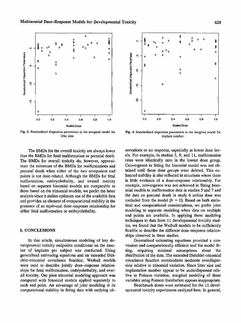
ond, the estimated values of K are often less than zero (only four standardized estimates of K in Fig. 3 are greater than 2), indicating that underdispersion is likely to occur relative to Poisson variation. This finding agrees with that in two previous reports.(loJ1) We also find that overdispersion tends to occur at higher doses which induce excessive prenatal deaths in some dams. Overall, Fig. 3 suggests a positive correlation between the value of K and dose.

A similar analysis of the implantation number rn was also conducted. Based on the estimates of t1 given in Table IV, implant number does not appear to be dose related. (Recall that implantation takes place before exposure in developmental toxicity studies.) In fact, re- moving dose from the model had little impact on model fitting. Figure 4 indicates that the Poisson distribution will not provide a good description of the variability in implant number among dams since underdispersion is clearly evident. This is due primarily to the natural bounds on implant number implied by the fact that a female rat or mouse would typically have about 6 to 18 implants.

10.0053)

5.3. Benchmark Doses

Benchmark doses corresponding to a 5 % excess risk level for malformations, prenatal death and overall toxicity based on both trinomial and binomial models are given in Table V. In general, the BMDs derived from the trinomial model are comparable with those from the binomial models. However, since the trinomial model utilizes all of the available information, it is expected to yield more precise estimates of the BMDs than the binomial models. This increased precision is reflected in the fact that the estimated standard errors associated with the trinomial model tend to be less than those associated with binomial models, although not uniformly so. The exceptions are due largely to the direct dependence of the approximate standard errors in (16) and (17) on the estimated parameter values and the impact of influential observations in experiments of moderate size. Note that for fetal malformations, the standard errors associated with the trinomial model are marginal with respect to s, whereas those associated with the binomial model are conditional on s.


I

00

0 0

0

0

0 0

O O

0

0.0 0.2 0.4 0.6 0.8 1 .o

Scaled Dose

Fig. 3. Standardized dispersion parameters in the marginal model for litter size.

The BMDs for the overall toxicity are always lower than the BMDs for fetal malformation or prenatal death. The BMDs for overall toxicity do, however, approximate the minimum of the BMDs for malformations and prenatal death when either of the two component end points is not dose-related. Although the BMDs for fetal malformation, embryolethality, and overall toxicity based on separate binomial models are comparable to those based on the trinomial models, we prefer the latter analysis since it makes optimum use of the available data and provides an element of computational stability in the presence of an equivocal dose-response relationship for either fetal malformation or embryolethality.

6. CONCLUSIONS

In this article, simultaneous modeling of key developmental toxicity endpoints conditional on the number of implants per subject was conducted. Using generalized estimating equations and an extended Diri- chlet-trinomial covariance function, Weibull models were used to describe jointly dose-response relationships for fetal malformation, embryolethality, and overall toxicity. Our joint trinomial modeling approach was compared with binomial models applied separately to each end point. An advantage of joint modeling is its computational stability in fitting data with outlying ob-

- 4 1 00 O

O 0 0

0 0 0 0 0

0

0

0

0

z o o 0

0 0

0

I I I I I I

0.0 0.2 0.4 0.6 0.8 1 .o

Scaled Dose

Fig. 4. Standardized dispersion parameters in the marginal model for implant number.

servations or no response, especially at lower dose levels. For example, in studies 3, 9, and 11, malformation rates were identically zero in the lowest dose group. Convergence in fitting the binomial model was not obtained until these dose groups were deleted. This en- hanced stability is also reflected in situations where there is little evidence of a dose-response relationship. For example, convergence was not achieved in fitting binomial models to malformation data in studies 5 and 7 and the data on prenatal death in study 6 unless dose was excluded from the model (b = 0). Based on both statistical and computational considerations, we prefer joint modeling to separate modeling when data on multiple end points are available. In applying these modeling techniques to data from 11 developmental toxicity studies, we found that the Weibull models to be sufficiently flexible to describe the different dose-response relationships observed in these studies.

Generalized estimating equations provided a con- venient and computationally efficient tool for model fitting, requiring minimal assumptions about the distribution of the data. The extended Dirichlet-trinomial covariance function accomodates moderate overdispersion relative to trinomial variation. Since litter size and implantation number appear to be underdispersed relative to Poisson variation, marginal modeling of these variables using Poisson distribution appears inappropriate.

Benchmark doses were estimated for the 11 developmental toxicity experiments analyzed here. In general,

626 Krewski and Zhu

Table V. Benchmark Doses (5%) Based on Trinomial and Binomial Dose-Response Models (Standard Error in Parentheses)

Fetal malformation Prenatal death Overall toxicity Study No. Unit Trinomial Binomial Trinomial Binomial Trinomial Binomial

1

2

3

4

5

6

7

8

9

10

11

426.37 (91.57)

1197.26 (164.99)

324.50 (50.25)

47.54 (13.19)

2685.23 (4484.16)

703.73 (63.95)

19.69 (2.15)

72.47 (16.27)

141.51 (27.82)

0.0398 (0.0058)

161.61 (12.32)

461.64 (81.86)

1182.41 (212.71)

371.16b (52.35)

44.57 (7.96) -

717.12 (68.86) -

74.94 (14.57)

149.57b (50.03)

0.0426 (0.0062)

157.6gb (13.17)

1823.88 (1030.92)

3379.83 (860.34)

454.48 (173.80)

61.50 (32.73)

1361.48 (182.67)

46121.0 (2 x 1oR)

17.03 (3.29)

110.67 (26.70)

132.24 (41.88)

0.0485 (0.0082)

219.22 (44.93)

1886.49 (1128.98)

3402.77 (636.07)

487.52 (186.25)

58.32 (37.29)

1380.13 (191.15) 4

12.16 (3.29)

113.19 (29.30)

100.35 (46.46)

0.0508 (0.0081)

218.87 (41.15)

401.01 (1 10.50)

1180.34 (164.33)

284.78 (59.65)

43.00 (14.78)

1284.73 (226.02)

703.64 (76.82)

16.56 (3.33)

66.27 (13.82)

114.97 (30.17)

0.0343 (0.0046)

146.59 (14.80)

404.12 (1 21.16)

1134.84 (220.36)

323.05 (55.65)

42.12 (15.22)

1326.82 (216.00)

73 1.48 (80.07)

15.58 (3.19)

66.10 (14.75)

106.69 (30.65)

0.0362 (0.0060)

144.22 (16.60)

a The binomial model could not be fit due to the lack of a dose-response relationship. The binomial model could not be fit until the second dose group of all zero rates was deleted.

the joint trinomial model would lead to more precise estimates of the BMDs than did separate binomial models. The BMDs based on overall toxicity were always below the minimum of the BMDs for fetal malformation and prenatal death, indicating the importance of consid- ering overall toxicity in risk assessment applications.

ACKNOWLEDGMENTS

This research was supported in part by Grant A8664 from the Natural Sciences and Engineering Re- search Council of Canada to D. Krewski. This paper was presented in part at the Annual Meeting of the Society for Risk Analysis in Baltimore, December 8-11, 1991, and at a Workshop on Quantitative Methods in Devel- opmental Toxicity sponsored by Health and Welfare Canada and the U.S. National Academy of Sciences in Ottawa, May 20-21, 1992. We are grateful to Dr. B. Schwez for providing the data analyzed in Section 5 and to Dr. D. Mattison for helpful comments. The referees’

constructive comments have improved the original presentation of this article.

REFERENCES

1.

2.

3.

4.

5.

6.

R. L. Kodell, R. B. Howe, J. J. Chen, and D. W. Gaylor, “Math- ematical Modeling of Reproductive and Developmental Toxic Ef- fects for Quantitative Risk Assessment,” Risk Anal. 11, 583-590

L. Ryan, “Quantitative Risk Assessment for Developmental Tox- icity,’’ Biometrics 48, 163-174 (1992). L. Ryan, “The Use of Generalized Estimating Equations for Risk Assessment in Developmental Toxicity,” Risk Anal. 12, 439-447 (1992). K. S. Crump, “A New Method for Determining Allowable Daily Intakes,” Fund. AppZ. Toxicol. 4, 854-871 (1984). Environmental Protection Agency, “Guidelines for Developmen- tal Toxicity Risk Assessment,” Fed. Register 56, 63797-63826

P. J. Catalan0 and L. Ryan, “Bivariate Latent Variable Models for Clustered Discrete and Continuous Outcomes,” J. Am. Stat.

(1991).

(1991).

Assoc. 87, 651658 (1992).

ed.) (Wiley, New York, 1981). 7. J. L. Fleiss, Statistical Methods for Rates and Proportions (2nd

Multinomial Dos+Response Models for Developmental Toxicity 627

8. J. J. Chen, R. L. Kodell, R. B. Howe, and D. W. Gaylor, “Anal- ysis of Trinomial Responses from Reproductive and Developmen- tal Toxicity Experiments,” Bwmetrics 47, 1049-1058 (1991).

9. K. Rai and J. Van Ryzin, “A Dose-Response Model for Terato- logical Experiments Involving Quanta1 Responses,” Biometrics 41, 825-839 (1985).

10. D. A. Williams, “Dose-Response Models for Teratological Ex- periments,” Biometrics 43, 1013-1016 (1987).

11. Y. Zhu, D. Krewski, and W. H. Ross, “Dose-Response Models for Correlated Multinomial Data from Developmental Toxicity Studies” (submitted for publication).

12. D. A. Williams, “The Analysis of Binary Responses from Toxi- cological Experiments Involving Reproduction and Teratogenic- ity,” Biometrics 31, 949-952 (1975).

13. D. A. Williams, “Extra-binomial Variation in Logistic Linear Models,” Appl. Stat. 31, la148 (1982).

14. L. L. Kupper, C. Portier, M. D. Hogan, and E. Yamamoto, “The Impact of Litter Effects on Dose-Response Modeling in Teratol- ogy,” Biometrics 42, 85-98 (1986).

15. J. J. Chen and R. L. Kodell, “Quantitative Risk Assessment for Teratological Effects,” J. Am. Stat. Assoc. 84, 966-971 (1989).

16. P. M. E. Altham, “Two Generalizations of the Binomial Distri- bution,’’ AppL Stat. 27, 162-167 (1978).

17. L. L. Kupper and J. K. Haseman, “The Use of a Correlated Bi- nomial Model for the Analysis of Certain Toxicological Experi- ments,” Biometriw 34, 69-76 (1978).

18. D. F. Moore, “Modelling the Extraneous Variation in the Pres- ence of Extra-Binomial Variaton,” Appl. Stat. 36, 8-14 (1987).

19. R. L. Prentice, “Binary Regression Using an Extended Beta-Bi- nomial Distribution, with Discussion of Correlation Induced by Covariate Measurement Errors,” J. Am. Stat. Assoc. 81, 321-327 (1986).

20. D. A. Williams, “Estimation Bias Using the Beta-Binomial Dis- tribution in Teratology,” Biometrics 44, 305-309 (1988).

21. K.-Y. Liang and S. Zeger, “Longitudinal Data Analysis Using Generalized Linear Models,” Biometrikn 73, 13-22 (1986).

22. R. L. Prentice, “Correlated Binary Regression with Covariate Specific to Each Binary Observation,” Biometrics 44, 1033-1048 (1988).

23. R. L. Prentice and L. P. Zhao, “Estimating Equations for Para- meters in Means and Covariances of Multivariate Discrete and Continuous Responses,” Biornetrics 47, 825-839 (1991).

24. D. F. Moore, “Asymptotic Properties of Moment Estimators for Overdispersed Counts and Proportions,” Eiometriku 73,583-588 (1986).

25. D. F. Moore and A. Tsiatis, “Robust Estimation of the Variance in Moment Methods for Extra-Binomial and Extra-Poisson Vari- ation,’’ Biometrics 47, 383401 (1991).

Applications of Multinomial Dose-Response Models in Developmental Toxicity Risk Assessment

Documents

Transcript of Applications of Multinomial Dose-Response Models in Developmental Toxicity Risk Assessment