
When do students intend to return? Determinants of students' return intentions using a multinomial...
40
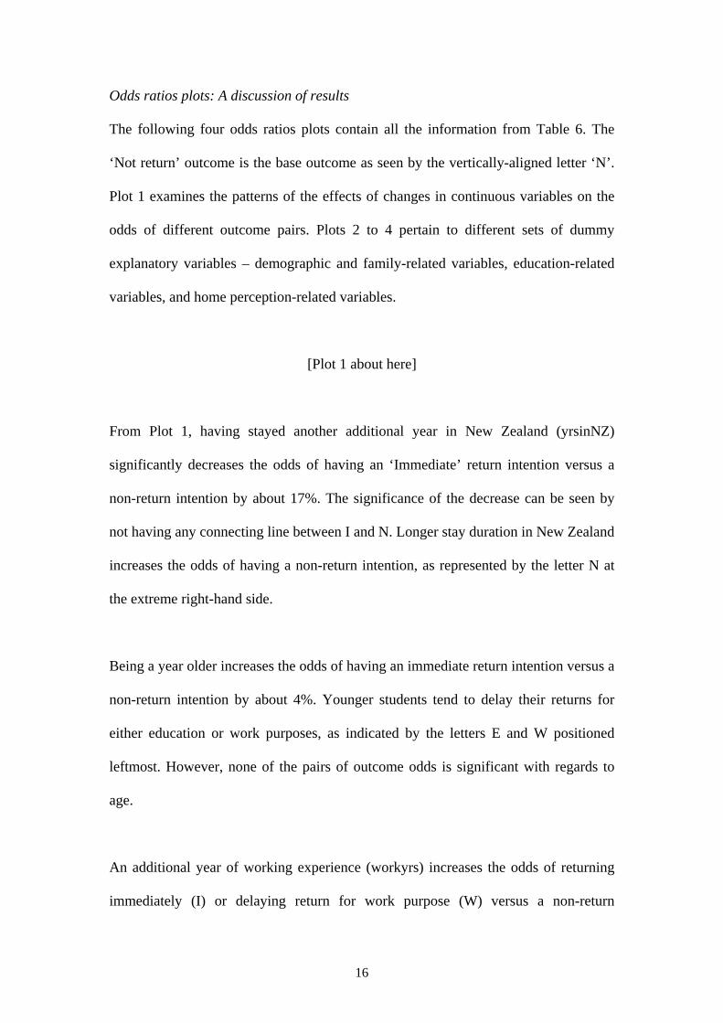
ISSN 1178-2293 (Online) University of Otago Economics Discussion Papers No. 0906 June 2009 When do students intend to return? Determinants of students’ return intentions using a multinomial logit model Jan-Jan, SOON ♣ Department of Economics University of Otago P.O.Box 56 Dunedin 9054 New Zealand Email: [email protected] Tel: 64-3-4797387 Fax: 64-3-4798174 ♣ I would like to express my gratitude to Robert Alexander and Murat Genç for their invaluable comments and insightful suggestions.
Transcript of When do students intend to return? Determinants of students' return intentions using a multinomial...

ISSN 1178-2293 (Online)
University of Otago Economics Discussion Papers
No. 0906
June 2009
When do students intend to return?
Determinants of students’ return intentions using a
multinomial logit model
Jan-Jan, SOON♣
Department of Economics University of Otago P.O.Box 56 Dunedin 9054 New Zealand Email: [email protected] Tel: 64-3-4797387 Fax: 64-3-4798174
♣ I would like to express my gratitude to Robert Alexander and Murat Genç for their invaluable comments and insightful suggestions.

Abstract
Using a multinomial logit model, this paper looks at the determinants of when tertiary
level international students intend to return home upon completion of their studies in
New Zealand, be it not return, return immediately, return after some working stint, or
return after some further education. Good perceptions of home have a strong positive
impact on the probability of returning immediately, with perception of home lifestyle
having the strongest impact. Contrary to received wisdom, perception of wage does
not play a dominant role in determining when students intend to return home.
JEL Classification: C25, J61
Keywords: Students’ migration, multinomial logit model, return intention

1
1.0 Introduction
Adapting Stark’s (2005) analogy, let there now be two orchestras in the world: a
mediocre orchestra (MO), and an excellent orchestra (EO). Suppose that an orchestra
player from the MO will have a chance to be admitted into the EO to learn more about
musicianship. Upon joining the EO, he has broader opportunities to learn from master
musicians, and more performance opportunities to hone his new-found skills.
Although the MO and the EO pay are similar, there are fewer learning and performing
opportunities available to him back at the MO. He now contemplates either not
returning at all or delaying his return to the MO.
This analogy strikes a chord with the questions addressed in this paper. This paper
looks at the return time frame of international students, that is, whether the students
intend to return immediately to their home countries after finishing their studies
abroad, to delay their return for some education or work purposes, or not to return at
all. The paper aims to identify the determinants of such intended return time frames.
Most students studying abroad intend not to return at all or to delay their return home
for work purposes. This is the main conclusion of this paper. This paper contributes to
the empirical literature by looking at when students intend to return home upon
completion of their current studies in New Zealand. Except for a handful of
qualitative studies (Baruch, Budhwar, & Khatri, 2007; Glaser, 1978), the students’
non-return literature lacks quantitative studies addressing the question of when
students return.

2
This paper differs from other studies in the students’ non-return literature which
typically look at whether or not students intend to return (Li, Findlay, Jowett, &
Skeldon, 1996) or at the intensity of their return intentions (Gungor & Tansel, 2008;
Zweig, 1997). In particular, this paper looks at when students intend to return home
upon completion of studies abroad, i.e., return immediately, delay their return for
work purposes, delay their return for educational purposes, or not return at all. Using a
multinomial logit model, the paper identifies the key determinants affecting such
intentions.
While most studies using discrete choice models interpret only the coefficient signs
and statistical significance, this study goes further to provide more comprehensive
interpretations, including those of different measures of marginal effects, changes in
outcome probabilities when variables of interest alter, and a graphical presentation of
the odds between outcome probabilities. This paper addresses the intricacies of a non-
linear model of when students intend to return.
The paper is organized as follows. The next section describes the dependent and
explanatory variables. Section 2 sets up the multinomial logit model, followed by two
specification tests. Section 3 discusses the main results in terms of discrete change
and odds ratios of outcomes. The following section looks at the robustness of the
model. The final section concludes.

3
1.1 Data
Individual level data are used in this study. These data are obtained through an online
questionnaire survey distributed via the two participating universities (Otago and
Canterbury) international offices. The survey was conducted between March and May
2007. There were 512 respondents from Otago and 269 from Canterbury, with
response rates of 20.17% and 11.7%. The lower response rate from Canterbury may
be due to the questionnaire’s being sent out just once instead of three times at Otago.
After excluding students who were bonded to return home, the final usable sample
totals 623 respondents.
The total number of the target population for this study is 20,515 international
students. Cavana et al (2001, p. 278) and Krejcie & Morgan (1970), suggest that a
sample size of 377 respondents is needed for a population size of 20,000. Hence, the
current study’s sample size of 623 respondents is adequate for the population of
international students considered. Soon (2008) gives further details of the survey used
to obtain the study’s sample.
1.2 Descriptive statistics
Table 1 shows the breakdown of the six outcome categories. These six outcome
categories are the alternatives available for the respondents in the survey
questionnaire used in data collection. The six alternatives are: whether a student
intends not to return at all (Not return), return immediately (Immediate), return after
an internship engagement (Internship), return after obtaining another degree (Degree),

4
return after gaining some working experience (Job) which is of a more short term
nature, or return after establishing a career (Career) which is of a more long term
nature. These alternatives eventually make up the multinomial (polychotomous)
dependent variable in this paper.
[Table 1 about here]
Due to some of the outcome categories having relatively few observations (e.g.,
Internship, Degree, and Career), the outcome categories are pooled into four
categories to make up the 4-outcomes dependent variable. The ‘Internship’ and
‘Degree’ categories are combined into one as ‘Education’, while the ‘Job’ and
‘Career’ categories as ‘Work’. For ease of interpretation, the four outcomes are
referred to as ‘Not return’ (n=284), ‘Immediate’ (n=115), ‘Education’
(n=48+31=79), and ‘Work’ (n=34+111=145). The ‘Education’ and ‘Work’
outcomes denote a delayed return intention. The pooling of the outcomes is formally
tested in Section 2.1.
Table 2 shows the breakdown of the explanatory variables by each of the four
outcomes. There are three sets of explanatory variables: personal and socio-economic
variables, education-related variables, and perception-related variables. Appendix A
supplies a brief description of both the dependent and explanatory variables.
[Table 2 about here]
5
Table 2 shows that about 45% of the students (respondents) have no intention to
return, 18% intend to return immediately, and the rest intend to delay their return,
either for education or work purposes. These are the actual sample proportions of the
students selecting one of the four outcomes. Those who intend to return immediately
are, on average, older (mean age = 26.2) than those who intend otherwise. Likewise
for those with the most work experience (mean years of work experience = 2.2).
Only about a quarter (26.5%) of those who initially intend to return (i.e. the
‘initialreturn’ variable) would return immediately, with a majority
(18.6+35.1=53.7%) of them intending to delay their return. More than half of the
students whose family supports their non-return intention do not intend to return
(55%). Half of the doctoral students (50.7%) have no intention to return. Likewise
50.7% of those who have been foreign-educated (i.e., the ‘hselsewhr’ variable) prior
to their current degree in New Zealand. Also, 56.8% of the health-science students
have no intention to return.
The perception-related variables are perceptions of six different aspects of the
students’ home countries. A third of those who have favourable perceptions on the
home working environment (goodHwenv; 33.1%), opportunities for knowledge use
(goodHoppk; 35.1%), and lifestyle (goodHlife; 33.3%), intend to return immediately.
However, 37.7% of those who have good perceptions of home wages, do not intend to
return.
6
2.0 Multinomial logit model specification
The multinomial logit (MNL) model is typically used when there is no clear-cut
ordering of the outcomes. The MNL model can be derived from random utility
maximization (RUM) theory. According to RUM theory, an individual (a decision-
maker) is assumed to choose the alternative that yields him the highest utility. His
utility can be described by a utility function. This function depends on the
characteristics of the individual. The utility function has a deterministic and a
stochastic component. The stochastic component is only relevant to the researcher, as
each individual is assumed to know perfectly the utility of each alternative (Manski,
1977).
Let the utility for a student i faced with J alternatives and choosing alternative m be:
immiimU ε+= βX (1)
The probability of choosing alternative m over other alternatives is when
( ) ( )ijimi UUPmYP >== mj ≠∀ (2)
In order to obtain the MNL model, the error term ε in equation (1) is assumed to be
independent and identically distributed (iid) with a Weibull (or type I extreme-value)
distribution (McFadden, 1974, p. 111), as follows:
( ) ( )[ ]εε −−= expexpF (3)

7
This type of error distribution results in the MNL model, where, given a set of
individual-specific characteristics iX , the probability of student i choosing alternative
m is:
( ) ( )( )∑
=
== J
jji
miii
exp
expmYP
1
|βX
βXX with 01 =β and mj ≠∀ (4)
The arbitrarily chosen 1β is set to zero (i.e. the base outcome category in the MNL
model) for the purpose of model identification. The coefficients of the remaining
outcome categories are interpreted relative to the base category. Equation (4) shows
that the outcome probabilities vary with changes in the explanatory variables in a non-
linear fashion.
The paper fits an MNL model with a 4-outcome dependent variable, such that,
1 if a ‘Not Return’ intention is stated
Y = 2 if an ‘Immediate’ intention is stated
3 if an ‘Education’ intention is stated
4 if a ‘Work’ intention is stated (5)
The ‘Not return’ outcome is chosen as the base outcome category because of its
intuitive nature. It serves as the reference point for all other outcome categories. This
outcome category is the only one which denotes a non-return intention, while the
other three outcome categories pertain to an intention to return, be it either an
immediate or a delayed return. The ‘Not return’ category also has the highest number
of observations.

8
2.1 Specification Test I: Pooling of outcomes
This section looks at how the outcomes can be pooled. A pair of outcomes can be
pooled if it is indistinguishable with respect to X . A pair of outcomes is
indistinguishable with respect to X if X does not significantly affect the odds of
outcome m versus outcome n (Anderson, 1984, p. 2).
Prior to the preferred 4-outcome model, 6-outcome and 3-outcome MNL models have
been fitted. The paper does not report the basic estimation results of the latter two
models. The pooling of outcomes tests are applied on all three specifications to
determine if any pairs of outcomes could be pooled further. The pooling of outcomes
can give a more parsimonious specification, which is especially critical in MNL
models where the parameters proliferate with the number of outcomes and
explanatory variables.
Table 3 shows three results panels. Each panel corresponds to a different specification
of the dependent variable. The Wald test and likelihood ratio (LR) test are used to test
for the hypothesis that a pair of outcomes can be combined. The pooling of outcomes
in MNL models was developed by Cramer & Ridder (1991), whereas the LR test for
such pooling was developed by Caudill (2000).
[Table 3 about here]
Insignificant tests indicate that two outcomes are indistinguishable. However, there
are some mixed results from the two types of test. For example, in the 6-outcome
9
specification, the insignificant Wald test suggests that the Career-Internship pair of
outcomes may be combined, while the significant (at 10% level) LR test suggests not.
In the 4-outcome specification, there are also competing results. The insignificant
Wald test suggests the pooling of the Education-Work pair, while the significant LR
test suggests otherwise. Since there are some mixed results from the tests, this paper
adopts a middle ground with the 4-outcome specification. The 4-outcome
specification is more parsimonious than the 6-outcome specification. At the same
time, it can discern more information than the 3-outcome specification. A 3-outcome
specification may obscure important information as to whether students prefer a
delayed return for education or for work purposes.
2.2 Specification Test II: Independence of irrelevant alternatives (IIA)
The Hausman-McFadden (HM) (1984) and Small-Hsiao (SH) (1985) tests are used to
test for the violation of the IIA property. Table 4 shows the results of the tests. Both
tests compare the estimated coefficients from the full model to those from a restricted
model that omits one of the alternatives. The null hypothesis to be tested is that the
odds between a pair of alternatives are independent of other alternatives.
[Table 4 about here]
The HM test shows negative chi-squared test statistics. Such negative test statistics are
common (Long & Freese, 2006, p. 244-5) and indicate that the IIA property is not
violated (Hausman & McFadden 1984, p. 1226). The results are further supported by

10
the SH test, where all the test statistics are insignificant, giving further evidence that
the IIA property holds.
The tests results suggest no IIA problem, indicating that the MNL model suits the data
in hand. The tests also indicate that the unobserved factors can be assumed to be
independent across alternatives, implying that the alternatives are dissimilar
(Amemiya, 1985, p. 298). Here, the tests results suggest that the students do not view
the four alternatives as close substitutes. Since the IIA property is not violated, the
four alternatives may be considered as dissimilar and distinct from one another.
Since no test can be conclusive, the best advice is to use an MNL model when the
alternatives are dissimilar (Amemiya, 1981, p. 1517) or when the alternatives can be
plausibly assumed to be distinct and weighed independently in the eyes of the
decision-maker (McFadden 1974, p. 113).
Having justified the use of a 4-outcome model and checked for the IIA assumption,
the next two sections discuss the main results from the MNL model. Note that, in
discussing the results from nonlinear discrete choice models such as the MNL model,
the coefficient estimates are rarely of interest in themselves, apart from the coefficient
sign and significance level.

11
3.0 Results discussion I: Discrete changes analysis
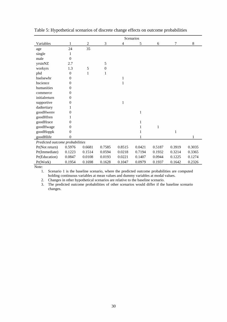
This section discusses the results in terms of discrete changes. Table 5 is an
alternative way to look at how a discrete change in a variable impacts the outcome
probabilities. A scenario depicts a hypothetical student with a certain set of
characteristics. Scenario 1 is the baseline scenario on which all subsequent
hypothetical scenarios are based. The baseline scenario is set at the mean values of
continuous variables and at the modal values of dummy variables. A student with the
set of characteristics in Scenario 1 observes the highest probability in having a non-
return intention, where Pr(Not return)=0.5976. The outcome probabilities of Scenario
1 serve as the benchmark probabilities, to which the outcome probabilities of other
scenarios are compared.
Scenario 2 depicts a hypothetical middle-aged female doctoral student who has been
working prior to coming to New Zealand for her (i.e., as indicated by the modal value
of male=0 from the baseline scenario) current study. All her other characteristics are
the same as in the baseline scenario. Her probability of having a non-return intention
has increased about 12% from the baseline probability of 0.5976 to the current
probability of 0.6681.
[Table 5 about here]
Scenario 3 depicts a 24 year old (the mean age of the sample) female doctoral student
with no working experience, and who has been staying in New Zealand for five years.
This scenario is typical of undergraduate honours students who continue directly with

12
their doctoral studies. Her probability of having a non-return intention has increased
about 27% from the baseline probability of 0.5976 to the current probability of
0.7585.
Scenario 4 depicts a female health science undergraduate who has studied abroad
before (hselsewhr=1), and whose family is supportive of her non-return intention. Her
probability of having a non-return intention has increased about 42% from the
baseline probability of 0.5976 to the current probability of 0.8515. A 42% increase in
Pr(Not return) is non-trivial, pointing out the important combined effect of changes in
those three variables (i.e., ‘hselsewhr’, ‘hscience’, and ‘supportive’).
Scenarios 2 to 4 show the factors (i.e., the variables or students’ characteristics) which
are important in increasing the probability of having a non-return intention. By
contrast, Scenario 5 depicts the factors that are important in affecting the intention to
return immediately. The hypothetical student in Scenario 5 has only good perceptions
of her home country. Her probability of intending to return immediately is now
0.7194, about six times higher than the baseline probability of 0.1223. The evidence
here lends support to the hypothesis that good perceptions of different aspects of
home have a large positive impact on return intentions.
The last three scenarios 6 to 8 dissect the impact of selected home perception
variables separately. Contrary to the received wisdom from the literature, good
perceptions of wage competitiveness at home (goodHwage) do not have as large an
impact as that of good perceptions of knowledge use opportunities at home
(goodHoppk) and good perceptions of home lifestyle (goodHlife). For example, a
13
good perception of home wage only increases the Pr(Y=Immediate) from 0.1223 to
0.1932, corresponding to an increase of about 58% in Pr(Y=Immediate). A good
perception on home lifestyle, on the other hand, increases the Pr(Y=Immediate) from
0.1223 to 0.3365, an increase of about 175% in Pr(Y=Immediate). This increase is
about three times as large as that caused by the good home wage perception. The
evidence here suggests that other aspects may be more important than wages in
affecting return intentions.
3.1 Results discussion II: Odds ratios analysis
In addition to discrete changes, we can also examine the odds ratios between
outcomes. An odds ratios analysis differs from a discrete change analysis in two ways.
First, discrete changes depend on the amount of change and the set of explanatory
variables examined. Second, discrete changes give only the level of outcome
probabilities, but not the odds of how likely one outcome is compared to another.
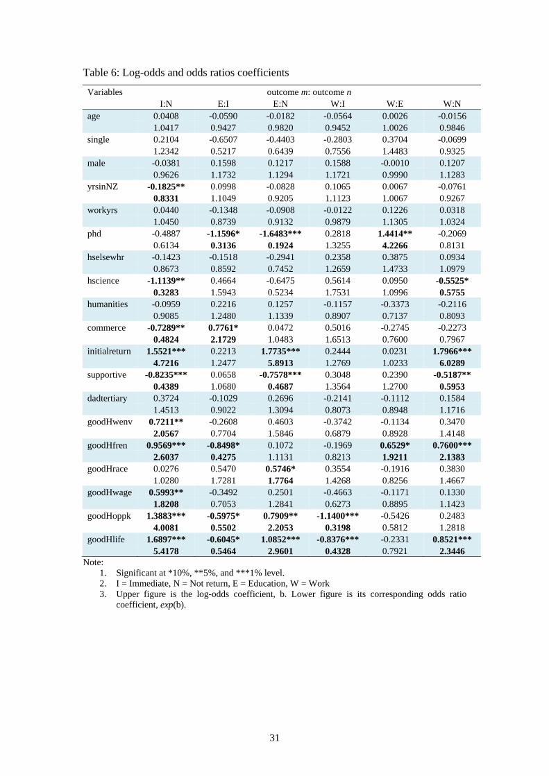
Table 6 shows the odds ratios for six pairs of outcomes. In the 4-outcome MNL
model, there are 12 pairs of outcomes. The odds ratios of the remaining six pairs of
outcomes can be easily computed from Table 6. For example, the log-odds coefficient
of age for the ‘Immediate: Not return’ outcome pair is 0.0408 with its corresponding
odds ratios coefficient of exp(0.0408)=1.0417. If the odds are inverted, then the log-
odds coefficient of age for the ‘Not return: Immediate’ outcome pair becomes -0.0408
with its corresponding odds ratios coefficient of exp(-0.0408)=0.96. The statistical
significance remains unchanged for the inverted odds.

14
[Table 6 about here]
For each additional year of residence in New Zealand, the odds of intending to return
immediately versus that of not returning decrease by a factor of 0.8331, or more
intuitively, decrease by about 17%, ceteris paribus. Alternatively, one can look at the
inverted odds. For each additional year of residence in New Zealand, the odds of
having no return intention versus that of to return immediately are about 1.2 times
greater, ceteris paribus, or equivalently, increase about 20%.
Even from the brief interpretation above, one can see the large number of
comparisons between outcomes. This makes it difficult to present interpretations in a
systematic manner. Furthermore, it is difficult to see if there are any patterns between
the odds and the variables just by eyeballing the table. A graphical presentation may
help delineate any existing patterns. An odds ratios plot holds the same tabular
information, in addition to drawing out patterns.
Odds ratios plots: An explanation
The odds ratios plot, originated by Long (1987), shows the patterns of the effects of
changes in the explanatory variables on the odds of different outcome pairs. The odds
ratio plot can keep track of the coefficient sign, the coefficient magnitude, and the
statistical significance as in its tabular counterpart. At the same time, it is superior to
the tabular form because it can extract patterns obscured in the table.
There are two scales on an odds ratio plot. The lower scale shows the log-odds
coefficients, while the upper scale shows its corresponding odds ratios coefficients.

15
Positive log-odds coefficients translate into odds ratios coefficients of more than one,
while odds ratios between zero and one are the counterparts of negative log-odds
coefficients.
A letter inside the plot denotes an outcome, so in order to avoid ambiguity, it is
advisable to use a different letter for each outcome. A letter lying straight along the
same vertical line denotes the selected base outcome. If a letter is to the right of
another letter, increases in an explanatory variable make the outcome to the right
more likely to occur. The horizontal position of a letter thus reflects the coefficient
sign.
The distance between a pair of letters (outcomes) indicates the magnitude of effects of
a change in an explanatory variable. The wider the distance, the larger the effects are.
The magnitude of effects can be read from either scale. The magnitude of effects is
typically measured relative to the base outcome. It is best to read the more accurate
magnitude from Table 6.
A connecting line between any two letters means that the odds of the two outcomes
are statistically insignificant with respect to the variable. The odds of a pair of
outcomes are statistically significant with respect to the variable when there is no
connecting line between the two letters. Note that there is no meaning to the vertical
distances between the letters. The vertical distances are to make the connecting lines
easily seen.
16
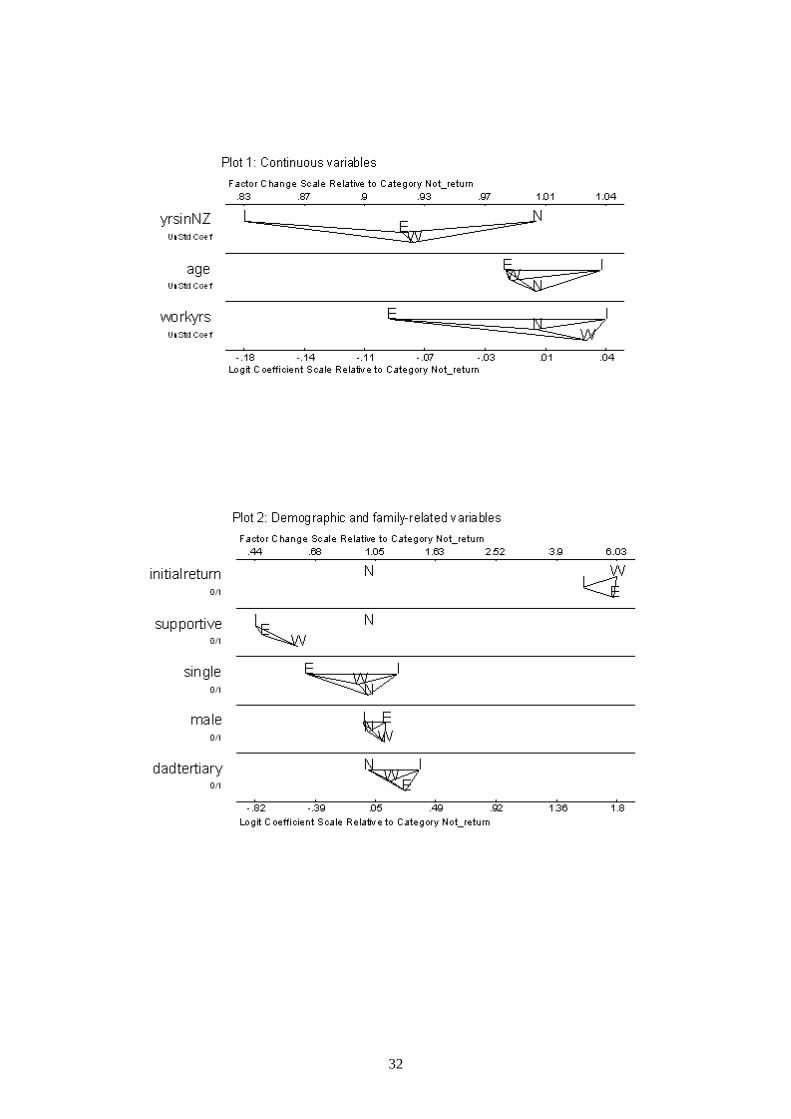
Odds ratios plots: A discussion of results
The following four odds ratios plots contain all the information from Table 6. The
‘Not return’ outcome is the base outcome as seen by the vertically-aligned letter ‘N’.
Plot 1 examines the patterns of the effects of changes in continuous variables on the
odds of different outcome pairs. Plots 2 to 4 pertain to different sets of dummy
explanatory variables – demographic and family-related variables, education-related
variables, and home perception-related variables.
[Plot 1 about here]
From Plot 1, having stayed another additional year in New Zealand (yrsinNZ)
significantly decreases the odds of having an ‘Immediate’ return intention versus a
non-return intention by about 17%. The significance of the decrease can be seen by
not having any connecting line between I and N. Longer stay duration in New Zealand
increases the odds of having a non-return intention, as represented by the letter N at
the extreme right-hand side.
Being a year older increases the odds of having an immediate return intention versus a
non-return intention by about 4%. Younger students tend to delay their returns for
either education or work purposes, as indicated by the letters E and W positioned
leftmost. However, none of the pairs of outcome odds is significant with regards to
age.
An additional year of working experience (workyrs) increases the odds of returning
immediately (I) or delaying return for work purpose (W) versus a non-return

17
intention. However, changes in age or in working experience are statistically
insignificant on the odds of all outcome pairs, as shown by the lines connecting each
of the outcomes.
[Plot 2 about here]
In Plot 2, for a student who initially intends to return (initialreturn), the odds of having
an immediate return intention versus a non-return intention are about 4.7 times
significantly higher than a student who has no such initial intention. The plot also
shows that a student who initially intends to return is significantly likelier to either
return immediately, or delay his return for work or education purposes than not return
at all. This is indicated by the cluster of I, W, and E on the right of N. However, there
is no statistical significance differentiating among the three I, W, and E intention
outcomes. A change in the ‘initialreturn’ variable has a large impact on the odds, as
indicated by the wide horizontal distance between N and other outcomes at the right-
hand cluster.
Due to the large odds magnitude exhibited by the initial intention variable, there may
be concern that this variable may be essentially measuring the same thing as the
dependent variable and should be excluded from the model. A restricted version
model is estimated (unreported here) without this variable and we found nontrivial
changes in coefficients magnitudes and signs. The correlation coefficient between the
‘initialreturn’ variable and the dependent variable is a relatively low 0.45. We further
performed a restriction test on the ‘initialreturn’ variable and found it to be

18
statistically significant at the 1% level. This suggests the inclusion of this variable in
the model.
In contrast to the ‘initialreturn’ variable, a change in the ‘supportive’ variable has a
somewhat smaller mirror image effect on the odds. A student whose family supports
his non-return intention increases his odds of a non-return intention versus other
return intentions. This is shown by the letter N on the far most right and the other
three outcomes clustered to the left. The odds of having an immediate return intention
versus a non-return intention significantly decrease by about 56% for a student with
such a supportive family.
The effects of the other three variables – being single, being a male, and coming from
a good socio-economic background (dadtertiary) – on the odds, are insignificant.
Besides being insignificant, the effects of these three variables have lower impacts, as
compared to those of the ‘initialreturn’ and ‘supportive’ variables. Lower impacts of
the effects can be seen from the smaller horizontal distances between two outcomes at
different ends.
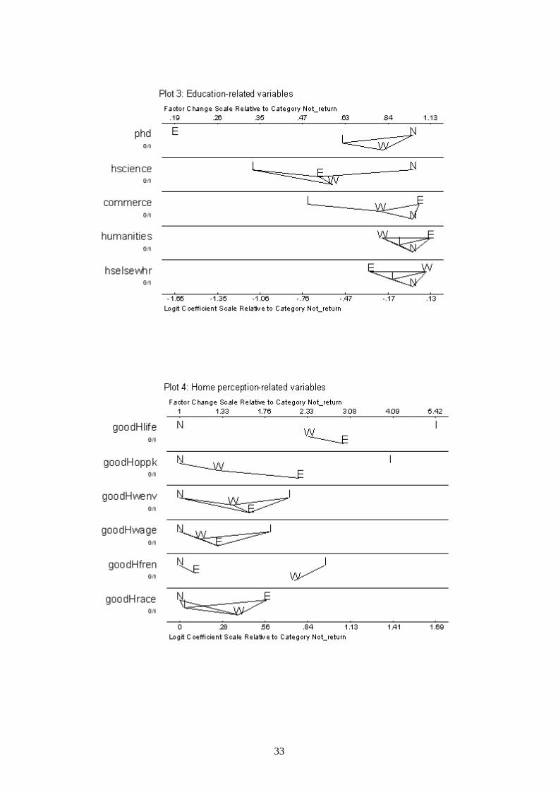
[Plot 3 about here]
Plot 3 shows that a doctoral student is most likely to have a non-return intention than
other return intentions. The odds of a doctoral student intending to delay return for
work purposes (W) versus that for education purposes (E) are about 4.2 times
significantly higher than a non-doctoral student. The E on the extreme left-hand side
indicates that doctoral students tend least to delay return for education purposes, as

19
compared to the other three return intentions clustered on the right-hand side. This
may be due to the nature of a doctoral study as a terminal degree.
Being a health science student (hscience), as compared to that of a science student,
significantly decreases his odds of having an immediate return intention versus a non-
return intention by about 67%. Or conversely, his odds of having a non-return
intention to that of returning immediately is about 3 times higher, ceteris paribus.
Simply put, he is more likely to have a non-return intention. This is indicated by the
letter N at the far end right.
Also, health science or commerce students, as compared to science students, are less
likely to intend to return immediately. This is indicated by the letter I at the far left
end. Being a student from the humanities discipline as compared to a science student,
does not have any impact on any pairs of odds. Whether or not a student has studied
abroad (hselsewhr) before also does not have any impact on any pairs of odds.
[Plot 4 about here]
Among the home perception-related variables shown in Plot 4, perceptions on home
lifestyle (goodHlife) have the largest impact on the odds of outcomes, as indicated by
its largest horizontal distance. For a student who prefers his home lifestyle, his odds
of having an immediate return intention versus a non-return intention are about 5.4
times significantly higher than a student who perceives otherwise. At the same time,
his odds of delaying his return for education and work purposes versus a non-return

20
intention are about 2.9 times and 2.3 times significantly higher than a student who
does not prefer the home lifestyle.
For a student who has good perceptions on knowledge use in his home country
(goodHoppk), his odds of having an immediate return intention versus a non-return
intention are about four times significantly higher than a student who perceives
otherwise. At the same time, his odds of delaying return for education purpose versus
a non-return intention are about 2.2 times significantly higher than otherwise.
However, the odds of the ‘Work-Not return’ pair are insignificant.
Plot 4 has a general pattern where all outcomes are on the right of N. This pattern
implies that, students who have good perceptions of their home countries, would
either intend to return immediately or to delay their return, rather than not returning at
all. Also note the similar patterns for four of the variables – goodHwenv, goodHwage,
goodHoppk, and goodHlife – where students with favourable perceptions of those
home aspects are most likely to return immediately, followed by delaying their return
for education purposes, and delaying their return for work purposes. A non-return
intention is the least of what they have in mind.
Contrary to the received wisdom from the literature, good perceptions on the wage
aspect in one’s home country (goodHwage) have one of the smallest impacts on the
odds, among the perception-related variables. The three perception variables that have
the largest impact are goodHlife, goodHoppk, and goodHfren, in that order.
Perceptions on race equality at home also do not have any significant impact on any
pairs of odds.

21
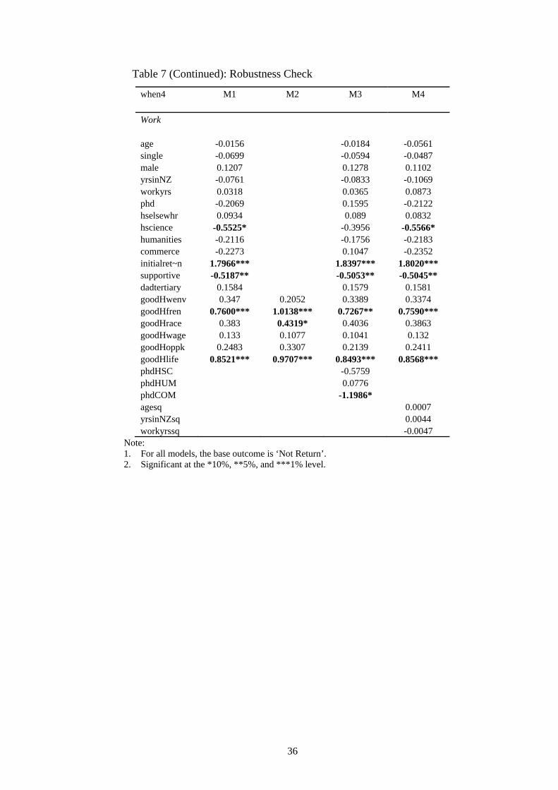
4.0 Robustness check
A robustness check gives an idea about the confidence one can place in the primary
model’s results. This section checks for the robustness of the paper’s primary model,
which is the MNL model with 4 outcome categories. The estimation results of three
different model specifications are compared with the results of the primary model for
substantial changes in key variables, either in the forms of different coefficient signs
or statistical significance.
Model M1 from Table 7 is the paper’s primary model. The estimated coefficients in
M1 are the log-odds coefficients. All coefficients signs and statistical significance in
the three result panels (Immediate, Education, Work) of models M1 to M4 are
interpreted relative to the base outcome – ‘Not return’.
[Table 7 about here]
Model M2 includes only the set of perception-related variables as its explanatory
variables. The coefficient signs of the significant variables are the same between M1
and M2, with some slight differences in the statistical significance of some of the
perception variables in each panel. While there is a danger of omitting important
variables in M2, this specification demonstrates the robustness of the conclusions that
can be drawn from perception-related variables.
Three interaction terms are added in the M3 specification. The doctoral level of study
is interacted with the disciplines of study. Only one of the interaction terms –

22
‘phdCOM’ in the ‘Work’ results panel – is significant at the 10% level. The signs and
significance of most key variables remains unchanged, with the exceptions of the
statistical significance of two disciplines of study variables: health science and
commerce. The primary model excluded interaction terms as there are no strong
theoretical reasons for their inclusion.
M4 takes on a different functional form in which it includes the squared terms of the
three continuous variables age, years of residence in New Zealand, and years of
working experience. None of the squared terms is significant and the results from M4
are essentially the same as the primary model M1. The statistical insignificance also
suggests no nonlinearity in the three continuous variables, that is, the outcome
probabilities do not exhibit reversing trends as these variables increase in values. The
primary model does not use any squared terms as there is no strong evidence for their
inclusion in the literature.
The robustness checks performed using M2 to M4 suggest that the results from the
primary model M1 are reasonably robust to changes in subsets of explanatory
variables (M2) and functional form (M3, M4). The discussion in this section suggests
that one can have considerable confidence in the primary model’s results.

23
5.0 Conclusions
As expected, a student with good perceptions of all the aspects of his home country
would be more likely to intend to return immediately after finishing his studies.
However, not all of the perceived aspects have the same effect on the outcome
probabilities or on the odds of the outcomes. Preference over one’s home lifestyle has
the largest positive impacts on a student’s intention to return immediately. Indeed, it
appears that the students want to return to familiar lifestyle, culture, and way of life.
Lifestyle preference, good opportunities for skills utilization, close-knit social ties,
good working environment at home are all more important than just high wages
offered by the home country. The first four factors are found to exert the largest
impact between choosing to return immediately or not to return at all. Therefore,
home governments seeking to attract return migration of scholars may need to re-
examine the return schemes to emphasize other aspects than just the pecuniary
compensation aspect. Failure to do so may result in lukewarm success of such
repatriation schemes.
Initial return intentions also have a large impact on the probabilities and the odds of
current return intentions. Students who initially intend to return tend either to return
immediately or delay their return, rather than not to return at all. A future extension of
the paper may look at whether there are changes in the initial return intentions and if
there are, what factors determine such changes.

24
Disciplines of study, especially the health science and commerce disciplines, have
positive impacts on a student’s intention not to return and negative impacts on a
student’s intention to return immediately. This may be due to these two disciplines
being unsuitable and irrelevant at the home country. For example, a student from the
health science discipline may be trained with technologies that are not available at his
home country, hence his inclination of not returning. The impacts of the disciplines of
study on delayed return intentions are generally not significant.
The factors examined here do not have any specifically large impacts on the
probability of a delayed return, be it a delay for education or work purposes. The
factors generally affect the most the intention of not returning. This may be an
indication that the permanent brain drain phenomenon is more pertinent than the less
damaging case of brain circulation.
One could question the use of intentions rather than observed behaviour as there may
be a divergence between intentions and actual subsequent behaviour. However,
divergence may simply reflect the dependence of behaviour on events not yet realized
at the time of survey (Manski, 1990, p. 940). That means, if there are no unexpected
events occurring between the time a person is asked of his intention and the time of
actual behaviour, then a person’s intention is the best prediction of his future
behaviour.
The paper contributes to the recent empirical students’ migration literature by looking
at the issue of the students’ intended return timeframe, instead of the more typical
question of whether or not they intend to return, or the intensity of their return

25
intention. The question of when students intend to return is crucial as it may translate
into either a permanent or a temporary brain drain issue for the home country.

26
Table 1: Outcome categories breakdown
When return n % Not return 284 45.59 Immediate 115 18.46 Internship 31 4.98 Degree 48 7.70 Job 111 17.82 Career 34 5.46 Total 623 100.00

27
Table 2: Descriptive statistics
4-outcome dependent variable Explanatory Variables
Not return Y=1
Immediate Y=2
Education Y=3
Work Y=4
Total
Continuous variables age 24.3 26.2 22.8 24.5 - yrsinNZ 3.0 2.1 2.9 2.6 - workyrs 1.1 2.2 0.5 1.4 - Dummy variables Demographic and socio-economic variables single 257 (45.9) 100 (17.9) 74 (13.2) 129 (23.0) 560 (89.9) male 134 (45.0) 52 (17.5) 38 (12.8) 74 (24.8) 298 (47.8) initialreturn 48 (19.8) 64 (26.5) 45 (18.6) 85 (35.1) 242 (38.8) supportive 166 (55.0) 42 (13.9) 30 (9.9) 64 (21.2) 302 (48.5) dadtertiary 182 (44.9) 76 (18.8) 54 (13.3) 93 (23.0) 405 (65.0) Education-related variables phd 78 (50.7) 34 (22.1) 5 (3.3) 37 (24.0) 154 (24.7) hselsewhr 142 (50.7) 36 (12.9) 35 (12.5) 67 (23.9) 280 (44.9) science* 105 (44.7) 48 (20.4) 25 (10.6) 57 (24.3) 235 (37.7) hscience 63 (56.8) 11 (9.9) 11 (9.9) 26 (23.4) 111 (17.8) humanities 52 (40.9) 32 (25.2) 18 (14.2) 25 (19.7) 127 (20.4) commerce 64 (42.7) 24 (16.0) 25 (16.7) 37 (24.7) 150 (24.1) Perception-related variables goodHwenv 42 (29.6) 47 (33.1) 22 (15.5) 31 (21.8) 142 (22.8) goodHfren 179 (38.7) 102 (22.0) 60 (13.0) 122 (26.4) 463 (74.3) goodHrace 85 (37.6) 38 (16.8) 39 (17.3) 64 (28.3) 226 (36.3) goodHwage 87 (37.7) 67 (29.0) 29 (12.6) 48 (20.8) 231 (37.1) goodHoppk 46 (26.9) 60 (35.1) 30 (17.5) 35 (20.5) 171 (27.5) goodHlife 36 (21.4) 56 (33.3) 30 (17.9) 46 (27.4) 168 (27.0) Total 284 (45.6) 115 (18.4) 79 (12.7) 145 (23.3) 623 (100.00)
Note: 1. n(%) 2. Mean figures (in years) for continuous variables. 3. A 4-outcome dependent variable, Y = 1, 2, 3, 4. 4. Row totals pertain to each explanatory variable, while column totals pertain to each outcome. 5. *The ‘Science’ discipline is the base group among the four disciplines of study.

28
Table 3: Tests for pooling of outcomes
Wald test LR test Outcome pairs chi2 df chi2 df 6-outcome specification Career-Job 17.44 19 19.45 19 Career-Degree 22.53 19 26.68 19 Career-Internship 21.74 19 28.23* 19 Career-Immediate 39.08*** 19 52.42*** 19 Career-Not retun 42.97*** 19 49.57*** 19 Job- Degree 17.09 19 19.51 19 Job-Internship 15.80 19 23.68 19 Job-Immediate 38.71*** 19 45.41*** 19 Job-Not return 83.32*** 19 102.84*** 19 Degree-Internship 16.20 19 18.82 19 Degree-Immediate 28.92* 19 36.11*** 19 Degree-Not return 75.34*** 19 93.80*** 19 Internship-Immediate 28.46* 19 44.57*** 19 Internship-Not return 42.84*** 19 53.73*** 19 Immediate-Not return 128.60*** 19 203.70*** 19 4-outcome specification Immediate-Education 39.76*** 19 52.71*** 19 Immediate-Work 50.26*** 19 60.67*** 19 Immediate-Not return 129.24*** 19 203.68*** 19 Education-Work 22.22 19 27.81* 19 Education-Not return 88.56*** 19 115.01*** 19 Work-Not return 92.13*** 19 116.30*** 19 3-outcome specification Immediate-Delayed 54.81*** 19 66.76*** 19 Immediate-Not return 129.73*** 19 204.11*** 19 Delayed-Not return 113.31*** 19 156.70*** 19
Note: 1. Significant at the *10%, **5%, and ***1% level. 2. H0: A pair of outcomes can be pooled as one. 3. An insignificant test indicates indistinguishability between a pair of
outcomes, suggesting pooling of the outcomes. A significant test suggests against pooling.
4. The 4-outcome specification pools the Degree-Internship pair as Education and Job-Career pair as Work.
5. The 3-outcome specification pools the Education-Work pair as Delayed.

29
Table 4: IIA tests
Omitted chi2 df P>chi2 evidence HM test Immediate -16.738 40 - - Education -5.599 40 - - Work -28.383 40 - - Not return -7.516 40 - - SH test Immediate 39.333 40 0.500 for H0 Education 33.538 40 0.755 for H0 Work 44.050 40 0.304 for H0 Not return 37.905 40 0.565 for H0
30
Table 5: Hypothetical scenarios of discrete change effects on outcome probabilities
Scenarios Variables 1 2 3 4 5 6 7 8 age 24 35 single 1 male 0 yrsinNZ 2.7 5 workyrs 1.3 5 0 phd 0 1 1 hselsewhr 0 1 hscience 0 1 humanities 0 commerce 0 initialreturn 0 supportive 0 1 dadtertiary 1 goodHwenv 0 1 goodHfren 1 goodHrace 0 1 goodHwage 0 1 1 goodHoppk 0 1 1 goodHlife 0 1 1 Predicted outcome probabilities Pr(Not return) 0.5976 0.6681 0.7585 0.8515 0.0421 0.5187 0.3919 0.3035 Pr(Immediate) 0.1223 0.1514 0.0594 0.0218 0.7194 0.1932 0.3214 0.3365 Pr(Education) 0.0847 0.0108 0.0193 0.0221 0.1407 0.0944 0.1225 0.1274 Pr(Work) 0.1954 0.1698 0.1628 0.1047 0.0979 0.1937 0.1642 0.2326
Note: 1. Scenario 1 is the baseline scenario, where the predicted outcome probabilities are computed
holding continuous variables at mean values and dummy variables at modal values. 2. Changes in other hypothetical scenarios are relative to the baseline scenario. 3. The predicted outcome probabilities of other scenarios would differ if the baseline scenario
changes.
31
Table 6: Log-odds and odds ratios coefficients
Variables outcome m: outcome n I:N E:I E:N W:I W:E W:N age 0.0408 -0.0590 -0.0182 -0.0564 0.0026 -0.0156 1.0417 0.9427 0.9820 0.9452 1.0026 0.9846 single 0.2104 -0.6507 -0.4403 -0.2803 0.3704 -0.0699 1.2342 0.5217 0.6439 0.7556 1.4483 0.9325 male -0.0381 0.1598 0.1217 0.1588 -0.0010 0.1207 0.9626 1.1732 1.1294 1.1721 0.9990 1.1283 yrsinNZ -0.1825** 0.0998 -0.0828 0.1065 0.0067 -0.0761 0.8331 1.1049 0.9205 1.1123 1.0067 0.9267 workyrs 0.0440 -0.1348 -0.0908 -0.0122 0.1226 0.0318 1.0450 0.8739 0.9132 0.9879 1.1305 1.0324 phd -0.4887 -1.1596* -1.6483*** 0.2818 1.4414** -0.2069 0.6134 0.3136 0.1924 1.3255 4.2266 0.8131 hselsewhr -0.1423 -0.1518 -0.2941 0.2358 0.3875 0.0934 0.8673 0.8592 0.7452 1.2659 1.4733 1.0979 hscience -1.1139** 0.4664 -0.6475 0.5614 0.0950 -0.5525* 0.3283 1.5943 0.5234 1.7531 1.0996 0.5755 humanities -0.0959 0.2216 0.1257 -0.1157 -0.3373 -0.2116 0.9085 1.2480 1.1339 0.8907 0.7137 0.8093 commerce -0.7289** 0.7761* 0.0472 0.5016 -0.2745 -0.2273 0.4824 2.1729 1.0483 1.6513 0.7600 0.7967 initialreturn 1.5521*** 0.2213 1.7735*** 0.2444 0.0231 1.7966*** 4.7216 1.2477 5.8913 1.2769 1.0233 6.0289 supportive -0.8235*** 0.0658 -0.7578*** 0.3048 0.2390 -0.5187** 0.4389 1.0680 0.4687 1.3564 1.2700 0.5953 dadtertiary 0.3724 -0.1029 0.2696 -0.2141 -0.1112 0.1584 1.4513 0.9022 1.3094 0.8073 0.8948 1.1716 goodHwenv 0.7211** -0.2608 0.4603 -0.3742 -0.1134 0.3470 2.0567 0.7704 1.5846 0.6879 0.8928 1.4148 goodHfren 0.9569*** -0.8498* 0.1072 -0.1969 0.6529* 0.7600*** 2.6037 0.4275 1.1131 0.8213 1.9211 2.1383 goodHrace 0.0276 0.5470 0.5746* 0.3554 -0.1916 0.3830 1.0280 1.7281 1.7764 1.4268 0.8256 1.4667 goodHwage 0.5993** -0.3492 0.2501 -0.4663 -0.1171 0.1330 1.8208 0.7053 1.2841 0.6273 0.8895 1.1423 goodHoppk 1.3883*** -0.5975* 0.7909** -1.1400*** -0.5426 0.2483 4.0081 0.5502 2.2053 0.3198 0.5812 1.2818 goodHlife 1.6897*** -0.6045* 1.0852*** -0.8376*** -0.2331 0.8521*** 5.4178 0.5464 2.9601 0.4328 0.7921 2.3446
Note: 1. Significant at *10%, **5%, and ***1% level. 2. I = Immediate, N = Not return, E = Education, W = Work 3. Upper figure is the log-odds coefficient, b. Lower figure is its corresponding odds ratio
coefficient, exp(b).
32
33

34
Table 7: Robustness Check
when4 M1 M2 M3 M4 Immediate
age 0.0408 0.0415 0.1296 single 0.2104 0.253 0.1627 male -0.0381 -0.024 -0.0665 yrsinNZ -0.1825** -0.1822** -0.3902** workyrs 0.044 0.0502 -0.0475 phd -0.4887 -0.1688 -0.4202 hselsewhr -0.1423 -0.1387 -0.108 hscience -1.1139** -1.0330* -1.0998** humanities -0.0959 0.0288 -0.1009 commerce -0.7289** -0.4583 -0.7043* initialret~n 1.5521*** 1.5708*** 1.5462*** supportive -0.8235*** -0.8195*** -0.8275*** dadtertiary 0.3724 0.374 0.3912 goodHwenv 0.7211** 0.5415* 0.7066** 0.7663** goodHfren 0.9569*** 1.3031*** 0.9496** 0.9833*** goodHrace 0.0276 -0.1514 0.0328 0.0405 goodHwage 0.5993** 0.8315*** 0.5782* 0.5868** goodHoppk 1.3883*** 1.3252*** 1.3677*** 1.4155*** goodHlife 1.6897*** 1.6530*** 1.6844*** 1.6866*** phdHSC -0.2421 phdHUM -0.3737 phdCOM -0.9432 agesq -0.0015 yrsinNZsq 0.0281 workyrssq 0.0065

35
Table 7 (Continued): Robustness Check
when4 M1 M2 M3 M4 Education
age -0.0181 -0.0243 0.1092 single -0.4403 -0.4618 -0.5143 male 0.1217 0.1147 0.1028 yrsinNZ -0.0828 -0.0869 -0.2674 workyrs -0.0908 -0.0886 -0.2022 phd -1.6483*** -1.7059** -1.5542*** hselsewhr -0.2941 -0.292 -0.2587 hscience -0.6475 -0.644 -0.6307 humanities 0.1257 0.1063 0.1218 commerce 0.0472 0.2168 0.0582 initialret~n 1.7735*** 1.8064*** 1.7726*** supportive -0.7578*** -0.7564*** -0.7657*** dadtertiary 0.2696 0.2599 0.2972 goodHwenv 0.4603 0.3145 0.4469 0.4909 goodHfren 0.1072 0.3995 0.0942 0.1232 goodHrace 0.5746* 0.6238** 0.5945* 0.6003* goodHwage 0.2501 0.171 0.2426 0.233 goodHoppk 0.7909** 0.9483*** 0.7638** 0.8171** goodHlife 1.0852*** 1.2020*** 1.0876*** 1.0870*** phdHSC 0.4915 phdHUM 0.8228 phdCOM -0.525 agesq -0.0025 yrsinNZsq 0.0228 workyrssq 0.0105
36
Table 7 (Continued): Robustness Check
when4 M1 M2 M3 M4 Work
age -0.0156 -0.0184 -0.0561 single -0.0699 -0.0594 -0.0487 male 0.1207 0.1278 0.1102 yrsinNZ -0.0761 -0.0833 -0.1069 workyrs 0.0318 0.0365 0.0873 phd -0.2069 0.1595 -0.2122 hselsewhr 0.0934 0.089 0.0832 hscience -0.5525* -0.3956 -0.5566* humanities -0.2116 -0.1756 -0.2183 commerce -0.2273 0.1047 -0.2352 initialret~n 1.7966*** 1.8397*** 1.8020*** supportive -0.5187** -0.5053** -0.5045** dadtertiary 0.1584 0.1579 0.1581 goodHwenv 0.347 0.2052 0.3389 0.3374 goodHfren 0.7600*** 1.0138*** 0.7267** 0.7590*** goodHrace 0.383 0.4319* 0.4036 0.3863 goodHwage 0.133 0.1077 0.1041 0.132 goodHoppk 0.2483 0.3307 0.2139 0.2411 goodHlife 0.8521*** 0.9707*** 0.8493*** 0.8568*** phdHSC -0.5759 phdHUM 0.0776 phdCOM -1.1986* agesq 0.0007 yrsinNZsq 0.0044 workyrssq -0.0047
Note: 1. For all models, the base outcome is ‘Not Return’. 2. Significant at the *10%, **5%, and ***1% level.

37
Appendix A: Variables’ description
Variable description Variable name Multinomial dependent variable when4 Intend not to return (Y=1; Not return) Intend to return immediately (Y=2; Immediate) Intend to return after some education stints (Y=3; Education) Intend to return after some working stints (Y=4; Work) Explanatory variables Continuous variables (in years) Age age Residence years/stay duration in New Zealand yrsinNZ Years of working experience at home country prior to current degree in New Zealand workyrs Categorical variables (binary dummies) Marital status single Gender male Level of study phd Have had studied abroad before hselsewhr Science-related discipline (reference group) science Health science-related discipline hscience Humanities-related discipline humanities Commerce-related discipline commerce Initial intention on returning prior to leaving home initialreturn Family support on non-return intention supportive Father's education level dadtertiary Good home country perception on wage competitiveness goodHwage Good home country perception on opportunities for knowledge use goodHoppk Good home country perception on working environment goodHwenv Good home country perception on lifestyle goodHlife Good home country perception on family bond and friends network goodHfren Good home country perception on race equality goodHrace
Note: Sample size, n = 623

38
References
Amemiya, T. (1981). Qualitative Response Models: A Survey. Journal of Economic Literature, 19(4), 1483-1536.
Amemiya, T. (1985). Advanced Econometrics. Oxford: Basil Blackwell. Anderson, J. A. (1984). Regression and Ordered Categorical Variables. Journal of the
Royal Statistical Society. Series B (Methodological), 46(1), 1-30. Baruch, Y., Budhwar, P. S., & Khatri, N. (2007). Brain drain: Inclination to stay
abroad after studies. Journal of World Business, 42(1), 99-112. Caudill, S. (2000). Pooling choices or categories in multinomial logit models.
Statistical Papers, 41(3), 353-358. Cavana, R. Y., Delahaye, B. L., & Sekaran, U. (2001). Applied business research:
Qualitative and quantitative methods. Sdyney: John Wiley & Sons. Cramer, J. S., & Ridder, G. (1991). Pooling states in the multinomial logit model.
Journal of Econometrics, 47(2-3), 267-272. Glaser, W. A. (1978). The brain drain: Emigration and return. Oxford: Pergamon
Press. Gungor, N. D., & Tansel, A. (2008). Brain drain from Turkey: an investigation of
students' return intentions. Applied Economics, 40, 3069-3087. Hausman, J., & McFadden, D. (1984). Specification Tests for the Multinomial Logit
Model. Econometrica, 52(5), 1219-1240. Krejcie, R. V., & Morgan, D. W. (1970). Determining sample size for research
activities. Educational and Psychological Measurement, 30, 607-610. Li, F. L. N., Findlay, A. M., Jowett, A. J., & Skeldon, R. (1996). Migrating to learn
and learning to migrate: A study of the experiences and intentions of international student migrants. International Journal of Population Geography, 2, 51-67.
Long, J. S. (1987). A graphical method for the interpretation of multinomial logit analysis. Sociological Methods Research, 15(4), 420-446.
Long, J. S., & Freese, J. (2006). Regression models for categorical dependent variables using Stata. Texas: Stata Press.
Manski, C. F. (1977). The structure of random utility models. Theory and Decision, 8, 229-254.
Manski, C. F. (1990). The Use of Intentions Data to Predict Behavior: A Best-Case Analysis. Journal of the American Statistical Association, 85(412), 934-940.
McFadden, D. (1974). Conditional logit analysis of qualitative choice behavior. In P. Zarembka (Ed.), Frontiers of Econometrics. New York: Academic Press.
Small, K. A., & Hsiao, C. (1985). Multinomial Logit Specification Tests. International Economic Review, 26(3), 619-627.
Soon, J.-J. (2008). The determinants of international students' return intention, Economics Discussion Papers 0806: Department of Economics, University of Otago.
Stark, O. (2005). The new economics of the brain drain. World Economics, 6(2), 137-140.
Zweig, D. (1997). To return or not to return? Politics vs. economics in. Studies in Comparative International Development, 32(1), 92-125.