www.elsevier.com/locate/forpol

Forest Policy and Economics 7 (2005) 1–24

Tropical deforestation: a multinomial logistic model and some

country-specific policy prescriptions

Krushna Mahapatraa, Shashi Kantb,*

aDepartment of Natural and Environmental Sciences, Mid Sweden University, Ostersund 831 25, SwedenbUniversity of Toronto, 33 Willcocks Street, Toronto, ON, Canada, M5S 3B3

Received 29 October 2002; received in revised form 21 May 2003; accepted 3 June 2003

Abstract

Three problems-one-way effect hypothesis, data and estimation problems-in the existing econometric models of global

deforestation are addressed, robustness of the results is tested and country-specific policy prescriptions, for five countries, are

suggested. A theoretical deforestation model is proposed by incorporating two-way effects of all explanatory variables, and

hypothesizing that the net effect of a variable may vary across regions. Deforestation is used as qualitative variable to address

the data problem. Multinomial logistic model is used to deal with estimation problems, and the results of multinomial logistic

are found to be more informative and robust compared to the results of binary logistic and ordinary least square (OLS) methods.

Growth in population, forest areas, agriculture and road construction are the main causes of deforestation in high deforesting

countries, but debt service growth, in addition to agriculture and road construction, are the main causes in medium deforesting

countries.

D 2003 Elsevier B.V. All rights reserved.

Keywords: Discrete variables; Multinomial Logistic regression; Interactive dummy variables; Multiple-choice models; Tropical deforestation

1. Introduction

Tropical forests are valued for the direct economic

benefits and for the host of intangible benefits

bestowed on society. Tropical wood products con-

tribute approximately US $ 100 billion annually,

about 0.5% of global gross domestic product (World

Commission on Forests and Sustainable Develop-

ment, 1998). During the 1990s, over 150 Non-wood

1389-9341/$ - see front matter D 2003 Elsevier B.V. All rights reserved.

doi:10.1016/S1389-9341(03)00064-9

* Corresponding author. Tel.: +1-416-978-6196; fax: +1-416-

978-3834.

E-mail addresses: krushna.mahapatra@utoronto.ca

(K. Mahapatra), Shashi.kant@utoronto.ca (S. Kant).

Forest Products (NWFP) were traded in international

markets, the estimated value of which ranged

between US$5 and US$10 billion per annum, in

addition to the value of NWFP traded in local

markets (Prebble, 1999). These forests occupying a

mere 13.54% of total land area (FAO, 1997) contain

approximately 70% of all species (WRI, 1996). In

addition, most of the 500 million people living in or

at the edge of these forests are fully dependent on

the forests not only for their livelihood, but also for

their cultural and spiritual values (Roper and Rob-

erts, 1999). Despite their continuing beneficial con-

tributions to mankind disappearance of tropical

forests is unabated. The Food and Agricultural

K. Mahapatra, S. Kant / Forest Policy and Economics 7 (2005) 1–242

Organization (FAO) has estimated the average annual

rates of tropical deforestation to be 14.63 and 12.91

Mha for the periods 1980–1990 and 1990–1995,

respectively. Myers (1994) has estimated that the

average annual deforestation in humid tropics was

approximately 13.2 Mha during late 1980s. Due to

its long-term dangerous consequences such as global

warming, biodiversity loss and soil degradation,

every section of the society is concerned about

tropical deforestation.

Since the early 1980s, Policy makers have

responded with several bilateral and multi-lateral

initiatives such as Tropical Forestry Action Plan,

International Tropical Timber Organization and For-

est Principles. Social scientists have focused their

attention on the analyses of the phenomenon of

tropical deforestation. As a consequence, there has

been a flood of tropical deforestation models in the

last decade. Kaimowitz and Angelson (1998) cate-

gorized economic models of deforestation, on the

basis of scale, into micro (household), meso

(regional) and macro (national) levels; and on the

basis of methodology, into analytical, simulation and

regression models. However, macro-level models,

especially the cross-national empirical models are

the most popular tools, and constitute the single

largest category of deforestation studies at present

(Kaimowitz and Angelson, 1998). The macro-level

models are critical for macro-level policies and

institutional arrangements, but most of these suffer

from many econometric problems. First, the main

and totally unaddressed problem of these models is

related to one-way hypothesis of the effect of causal

variables on deforestation. Second, two other prob-

lems, which have been discussed, but not addressed

adequately in literature, are data and estimation

problems. Data problem arises due to quality of

data, and the statistical results derived from these

models can be dismissed as not being based on a

strong enough data (Kummer and Sham 1994).

Estimation problems have many sources such as

mis-specification of the model, limited degrees of

freedom, multi-collinearity and heteroscedasticity

(Kaimowitz and Angelson, 1998). Some studies have

attempted to address the second set of problems. For

example, Rudel and Roper (1997a) attempted to

address the data problem, and Kant and Redantz

(1997) dealt with some of the estimation problems.

However, no study has attempted to address all three

problems together.

In this article, our main objective is to demonstrate

that even with the available deforestation data useful

and consistent policy conclusions can be made pro-

vided, analysis is based on sound economic reasoning

and appropriate econometric techniques have been

used for the analysis. The focus of the article is on

the problems of hypothesis, data and estimation.

However, a test for the robustness of estimation

results to variation in the data on deforestation rates

and an attempt to prioritize the importance of causal

variables of deforestation to suggest country-specific

policy interventions are two other key features of the

article.

To put this in perspective, an overview of three

problems of deforestation models is provided in

Section 2. A theoretical deforestation model that

encompasses two-way effects of each causal

(explanatory) variable is presented in Section 3. In

Section 4, it is proposed that the dependent variable

of deforestation should be treated as a discrete or a

qualitative variable to deal with the subjective

accuracy of deforestation data. Three econometric

methods of model estimation—multinomial logistic,

binomial logistic and ordinary least squares

(OLS)—are discussed in Section 5. Data and data

sources for deforestation and explanatory variables

are given in Section 6. Estimated results of defor-

estation model obtained from multinomial logistic,

binomial logistics and OLS are compared, and the

stability of the results, with respect to some varia-

tions in deforestation data, is presented in Section

7. The results of most appropriate method-multi-

nomial logistic—are discussed in Section 8. Coun-

try specific policy priorities are then identified in

Section 9. Finally, article is concluded with some

observations about deforestation models and their

use.

2. Problems of deforestation models

2.1. Hypothesis problem

A causal variable may have both-positive and

negative-effects on deforestation through different

mechanisms, and the positive effect may outweigh

K. Mahapatra, S. Kant / Forest Policy and Economics 7 (2005) 1–24 3

the negative effect in one situation, and negative

effect may outweigh the positive effect in another

situation. Hence, the net effect of the same inde-

pendent variable may vary across different situa-

tions. For illustration, take the example of effect of

higher income on deforestation. Some authors have

hypothesized that higher income increases demand

for agricultural and forest products, which in turn

put greater pressure on forests, leading to defores-

tation (Kant and Redantz, 1997; Capistrano, 1990).

Others have hypothesized that higher income cre-

ates more off-farm employment away from the

agricultural frontier and develop awareness for

conservation of forests, and hence reduces defores-

tation (Angelson, 1999). But, both of these effects

may be operating simultaneously, and the domi-

nance of one effect over the other effect cannot be

determined a-priori. However, the majority of defor-

estation models have hypothesized ‘one-way effect’

causal mechanism and tested the posited hypothesis

(Rudel and Roper, 1997a,b; Kant and Redantz,

1997; Didia, 1997; Deacon, 1994) using one-tailed

t-test. Other deforestation models have used two-

tailed t-test (Rudel, 1989; Inman, 1993; Shafik,

1994). The two-tailed t-test recognizes the net effect

phenomenon, but the authors have not used it to

explore the different effects of a causal variable

across countries/regions. In this article, we propose

a deforestation model incorporating both positive

and negative effects of all independent variables

included in the model.

2.2. Data problem

Data problems are rooted in the definition of

deforestation and the varying methods of obtaining

data. Definitions of deforestation have been catego-

rized into ‘broad’ and ‘narrow’ types (Wunder,

2000). The broad version includes forestland use

conversion and forest degradation or reduction in

forest quality (density and structure, ecological

services, biomass stocks, species diversity etc.) while

the narrow version focuses only on change in forest-

land use. The FAO uses the narrow version and

defines deforestation as a ‘change in land use with

depletion of crown cover to less than 10%’ (FAO,

1993). The problem with this definition is that a loss

of crown density from a higher level such as 90% to

a level just above 10% will be considered as degra-

dation and not deforestation (Saxena et al., 1997).

Degradation and deforestation tend to be intertwined

phenomena in the sense that the former often pre-

cedes the latter (Wunder, 2000). However, technical

and financial constraints of developing countries are

the limiting factors in measuring forest degradation

and it does not seem to be avoidable in the near

future. Hence, present studies, including this study,

have to be focused on the narrow definition of

deforestation.

Even with the same definition of deforestation,

the estimation of deforestation (or forest area) differs

in different data sources including that of FAO. This

difference is mainly due to non-uniformity of the

categories of forest included and methods of data

collection. The FAO Production Yearbooks include

all forest and woodland, whether it is open or

closed, coniferous or broad-leaved (Kimsey, 1991),

while Forest Resource Assessment (FRA) data sets

of 1990 (FAO, 1993), FAO (1997) (revised estimate

of FRA, 1990; FAO, 1997) and 2000; (FAO, 2001)

include only tropical closed and broad-leaved forests

in estimating the forest loss. The FAO Production

Yearbook compiles data on land use, especially

forest area, based on national governments’ response

to annual questionnaires without any empirical basis.

National governments’ often have incentives to over

report the actual forest area (Shafik, 1994). Hence,

this data source is not reliable. FRA, 1990 is based

on inventories (either manual or based on remote

sensing data) of forest area from different countries.

Number of inventories varies from one to three

across countries. An ‘ecological deforestation model’

has been used to circumvent the problems of the

lack of two or more inventories from a country and

variation in years for which two inventories were

available for different countries. This model corre-

lates forest cover change in time with other varia-

bles including population density and population

growth for the corresponding period, initial forest

cover and the ecological zone (the model parameters

are different for different ecological zones at sub-

national level) under consideration (FAO, 1993).

The deforestation estimates for each ecological zone

at a sub-national level is aggregated at national level

to find the total deforestation. FRA, 1990 estimates

have been criticized for using population variable as

K. Mahapatra, S. Kant / Forest Policy and Economics 7 (2005) 1–244

independent variable in the ‘ecological deforestation

model’ that generates the deforestation data. Palo

(1999), however, claims that such criticisms are

exaggerated. He asserts that the population variable

plays a minor role in the model where lagged forest

cover and ecological zone variables (model param-

eters are different for different ecological zones)

explained more than 90% of the variation. The

forest area information in FRA, 2000 is based on

expert opinion and satellite imageries. Due to differ-

ent methodologies used in the FRA, 1990 and FRA,

2000, the two deforestation estimates should not be

compared (Matthews, 2001). Hence, all deforestation

data sources are questionable, and we propose in

Section 4, that deforestation should be used as a

discrete and not continuous variable.

2.3. Estimation problem

One of the main estimation problems of deforesta-

tion models is the combined use of direct and under-

lying causes as explanatory variables, which results in

mis-specification of the model and erroneous results.

For instance, suppose, Y is extent of deforestation, is

an average annual growth in area under cropland, the

direct cause of deforestation, and is an average annual

growth in population, the underlying cause of defor-

estation. Mathematical expression, when these two

causes are used together as explanatory variables of

deforestation is:

Y ¼ bo þ b1X1 þ b2X2 þ e ð1Þ

In such specification, the ceteris paribus effect of

population growth on deforestation is given by b2,

which is the case in studies such as Allen and Barnes

(1985), Bawa and Dayanandan (1997) and Tole

(1998). Change in cropland area, however, is a direct

cause of deforestation and a function of population

growth, which is an indirect or underlying cause of

deforestation. Mathematically,

X1 ¼ ao þ a1X2 þ e1 ð2Þ

Or

Y ¼ b0 þ b1aoð Þ þ b2 þ b1a1ð ÞX2 þ eþ b1e1ð Þ ð3Þ

Hence, the actual effect of X2 on deforestation is

b2+ 1a1, but the estimation of Eq. (1) gives only b2.

Kant and Redantz (1997) have used the two-stage

least square estimation procedure to address this

problem. However, in their study the effect of an

underlying cause on deforestation is determined

through its effects on different direct causes. The

direct causes are treated as independent of each other

while using some of the same underlying causes for

explaining direct causes, i.e. there is a problem of

simultaneity.

Two other estimation problems of deforestation

models are the correction for heteroscedasticity

and the incorporation of variations in the effect

of explanatory variables on deforestation across

regions. Heteroscedasticity is most common in

cross-sectional studies, and it may lead to an

explanatory variable to be insignificant (because

of low t-values), while it is not so. Most defor-

estation models have ignored this aspect, except a

few such as Capistrano (1990) and Kant and

Redantz (1997). Similarly, several studies, exclud-

ing Kant and Redantz (1997), have used only

dummy variables, and not interactive regional

dummy variables, which means the effect of

explanatory variables on deforestation is the same

across regions, which is not realistic (Kaimowitz

and Angelson, 1998). Other overlooked dimension

of methodological problems might be the assump-

tion of linearity in the relationship between the

deforestation and its explanatory variables. Some

evidence to this issue is provided by the results

indicating the presence of ‘Environment Kuznets

Curve’ phenomenon related to the relationship

between extent of deforestation and level of

national income (Cropper and Griffiths, 1994).

Solutions to these problems are discussed in

Section 5.

3. A model of tropical deforestation

Deforestation is a complex process where differ-

ent causal factors have their roots in different

sectors. While it seems that direct causes such as

agriculture/pasture expansion and forest products

consumption/export are driving deforestation (Sha-

fik, 1994), it is the underlying causes such as

K. Mahapatra, S. Kant / Forest Policy and Economics 7 (2005) 1–24 5

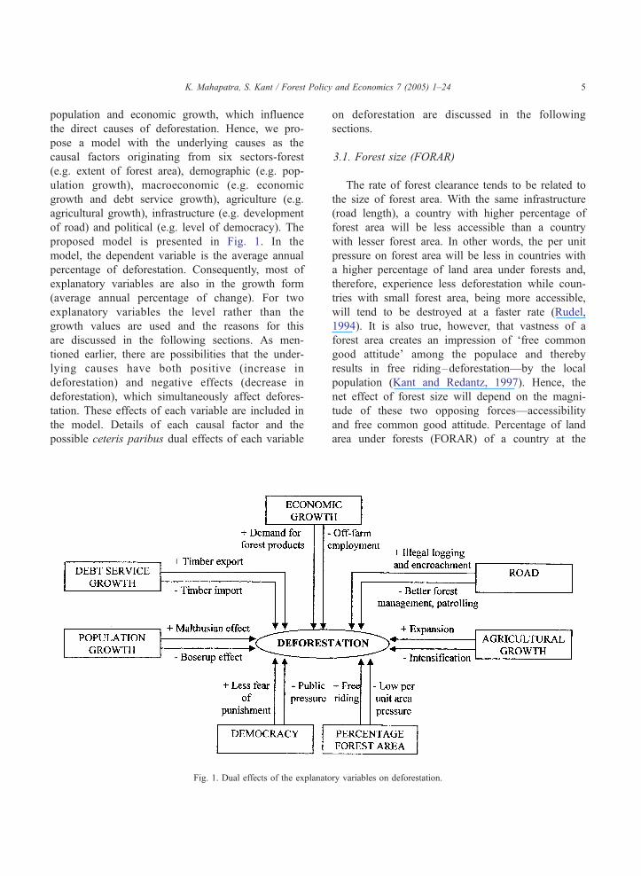
population and economic growth, which influence

the direct causes of deforestation. Hence, we pro-

pose a model with the underlying causes as the

causal factors originating from six sectors-forest

(e.g. extent of forest area), demographic (e.g. pop-

ulation growth), macroeconomic (e.g. economic

growth and debt service growth), agriculture (e.g.

agricultural growth), infrastructure (e.g. development

of road) and political (e.g. level of democracy). The

proposed model is presented in Fig. 1. In the

model, the dependent variable is the average annual

percentage of deforestation. Consequently, most of

explanatory variables are also in the growth form

(average annual percentage of change). For two

explanatory variables the level rather than the

growth values are used and the reasons for this

are discussed in the following sections. As men-

tioned earlier, there are possibilities that the under-

lying causes have both positive (increase in

deforestation) and negative effects (decrease in

deforestation), which simultaneously affect defores-

tation. These effects of each variable are included in

the model. Details of each causal factor and the

possible ceteris paribus dual effects of each variable

Fig. 1. Dual effects of the explanato

on deforestation are discussed in the following

sections.

3.1. Forest size (FORAR)

The rate of forest clearance tends to be related to

the size of forest area. With the same infrastructure

(road length), a country with higher percentage of

forest area will be less accessible than a country

with lesser forest area. In other words, the per unit

pressure on forest area will be less in countries with

a higher percentage of land area under forests and,

therefore, experience less deforestation while coun-

tries with small forest area, being more accessible,

will tend to be destroyed at a faster rate (Rudel,

1994). It is also true, however, that vastness of a

forest area creates an impression of ‘free common

good attitude’ among the populace and thereby

results in free riding–deforestation—by the local

population (Kant and Redantz, 1997). Hence, the

net effect of forest size will depend on the magni-

tude of these two opposing forces—accessibility

and free common good attitude. Percentage of land

area under forests (FORAR) of a country at the

ry variables on deforestation.

K. Mahapatra, S. Kant / Forest Policy and Economics 7 (2005) 1–246

beginning of the period is an ideal indicator of the

forest size of a country1. There cannot be a growth

variable for this factor because average annual rate

of change in forest area is the average annual rate

of deforestation, the dependent variable.

3.2. Population growth (POPGR)

Population growth is widely cited as the main

cause of tropical deforestation. Two centuries ago,

Malthus argued that increasing human population

will put severe pressure on natural resources such

as land and forests (Palo, 1994), and the UN

Environment Conference in Stockholm held in

1972 reinforced this view (Sayer, 1995). In economic

terms, decreased real wage rates and forest conver-

sion costs due to increased labor supply and higher

prices of agriculture land and agricultural products

due to increased demand of both, create economic

incentives to expand agriculture into forest areas

leading to deforestation (Wunder, 2000). This per-

spective has been supported by the positive correla-

tions found between population growth and

deforestation (Palo et al., 1996; Rudel and Roper,

1996; Southgate, 1994). However, according to

Boserup arguments, more people mean more crea-

tivity and ideas leading to development of new

technologies to cope with resource scarcity, and

higher labor absorption capacity in the agricultural

sector (Bilsborrow and Geores, 1994). In addition, a

rising population accelerates migration of rural peo-

ple to urban areas, plummeting pressure on forest

areas (Bilsborrow and Geores, 1994). The demand

for shelter in urban areas is met either by construct-

ing high-rise buildings or by developing new town-

ships in fallow lands around the existing city. These

viewpoints have been strengthened by the results

from deforestation studies that show negative (Bur-

gess, 1991) or no effect (Allen and Barnes, 1985;

Palo, 1994) of population growth on deforestation.

1 In data analysis this variable does not discriminate countries

based on the extent of total forest cover. For example, a large

country (India) with large forest area has the same importance in the

analysis as that of a small country (Nepal) with small forest area. In

other words, this variable accounts for the size of the country and

reduces the chances of heteroscedasticity.

Hence, as per the Neo-Malthusian proposition, at

constant agricultural growth (ceteris paribus condi-

tion in our model), a rise in population growth will

increase deforestation because of the demand of land

for shelter and illegal logging for income generation,

but not for food production. In contrast, an increase

in population growth will have a negative or no

effect on deforestation due to labor-intensive agri-

culture (Boserup hypothesis), more skills and tech-

nology and out-migration from rural areas.

3.3. Economic growth (GDPGR)

The dominant economic view is that low levels of

income and a lack of access to capital, force people to

be risk averse and adopt a high discount rate in

utilizing natural resources such as forests that leads

to deforestation (Lumely, 1997). Resource scarcities

due to deforestation make farmers poorer, and push

them further into new areas expanding deforestation.

This phenomenon is known as ‘immiserization

theory’, which goes back to Myrdal (1957), but it

was also highlighted in the Brundtland Commission

on Environment and Development (1987) that says:

‘those who are poor and hungry will often destroy

their immediate environment in order to survive. They

will cut down forests; their livestock will overgraze

lands; and they will overuse marginal lands’. Eco-

nomic growth creates ample off-farm employment

opportunities away from the frontiers that divert the

farmers from clearing the forests (Angelson, 1999).

Besides, availability of capital helps in better forest

management and creates awareness among citizens for

forest preservation (Capistrano, 1990). Hence, an

increase in income due to economic growth is

expected to reduce deforestation, and Rudel and

Roper (1997a) provide empirical evidence to support

this argument.

In contrast, the rising economic growth can also

have detrimental effects on deforestation. The

amount of local capital available for investment

in forest regions (for logging) increases with eco-

nomic growth leading to deforestation (Rudel and

Roper, 1996). Following loggers, peasants and land

speculators encroach the cleared forestland to

enforce their property rights. Pressures of these

groups on the surrounding forests along with the

unsustainable logging practice of loggers exacerbate

K. Mahapatra, S. Kant / Forest Policy and Economics 7 (2005) 1–24 7

the extent of deforestation. This is known as the

‘frontier theory’ of deforestation. Economic growth

also increases demand for agricultural and forest

products, both for domestic consumption and

export (Kant and Redantz, 1997). Expansion of

agricultural area and logging is necessary to meet

these increased demands, thus deforestation

increases.

Because growth in agriculture is taken as an

independent variable to study the effect of the agri-

cultural sector on deforestation, the growth rate of

Gross Domestic Product excluding the contribution of

agriculture (GDPGR) is used as an explanatory vari-

able to capture the effect of economic growth on

tropical deforestation.

3.4. Debt service growth (DEBTGR)

External debt is considered as one of the under-

lying factors driving tropical forest conversion (World

Bank, 1990). A basic hypothesis is that high external

debt service obligations push countries to make

myopic decisions in order to increase export of

primary products ignoring long-term natural resources

concerns (Leonard, 1985; Kahn and McDonanld,

1994). Such decisions may include economic incen-

tives, in terms of reduced timber prices, taxes and

other inputs at low prices, to increase production and

export of timber. Similarly, agriculture and re-settle-

ment policies may promote expansion of agricultural

areas into forest areas to increase foreign exchange

earnings from exports of agriculture products. Capital

scarcity also leads to low or no investment in forest

research and management. All these policies will

result into increased deforestation. However, develop-

ing countries in general depend on credit for almost

everything they import, and some countries may use

debt for importing timber and other forest-based

products such as pulp, paper and furniture. Similarly,

some countries may use the debt for alternate energy

sectors (reducing fuel wood consumption), improved

machines for wood processing (reducing wood

waste), forestry activities (e.g. research on sustainable

forest management) and plantations. All these activ-

ities will reduce the burden on forests, and thus,

deforestation.

Total debt service irrespective of the size of

economy (GNP) may not be an appropriate variable

to capture the effect of debt service on deforestation.

Because, if the debt service rises at the same rate as

growth in the economy, its pressure on natural resour-

ces may remain unaltered. Hence, we choose growth

rate of total debt service as a percentage of GNP

(DEBTGR) as an indicator of the pressure of debt

service on forest resources.

3.5. Agricultural growth (AGGR)

Two significant sources of agricultural growth

are the expansion of agricultural areas and intensi-

fication of agricultural practices. The two sources of

the expansion of agriculture into forest areas are

commercial agriculture and shifting cultivation.

Commercial agriculture such as sugarcane, tea,

coffee, cocoa, palm oil, rubber and coca production

in the nineteenth and twentieth centuries was

accomplished by clearing primary forests (Barra-

clough and Ghimire, 1995). This expansion has

resulted in the displacement of peasants from their

land to forested areas. World Bank (1992) asserts

that new settlement for agriculture accounts for 60%

of tropical deforestation. As well, cattle ranching

have been a major source of deforestation, partic-

ularly in Central and South America (Wunder,

2000). Approximately 85% of the deforestation in

the Brazilian Amazon is caused by some 5000

ranch-owners (Sponsel et al., 1996). Additionally,

slash-and-burn agriculture primarily for self-provi-

sioning by forest dwellers, migrants or peasants, is

frequently blamed for deforestation. In some South-

east Asian countries, shifting cultivation accounts

for up to 50% of natural forest conversion and 70%

in tropical West Africa/semiarid Africa (Rowe et al.,

1992). Hence, expansion of agriculture increases

deforestation. But, increased agricultural production

can also be achieved by agricultural intensification

such as increased use of fertilizer, pesticides, irri-

gation facility and new hybrid varieties (Bilsborrow

and Geores, 1994). Similarly, improved technology

often makes it possible to develop marginal lands

for crop production, and thus reducing the pressure

on forestland for extension of agriculture. Therefore,

intensification decreases deforestation and the net

effect of agricultural growth will depend upon

combined effect of expansion and intensification

of agriculture.

K. Mahapatra, S. Kant / Forest Policy and Economics 7 (2005) 1–248

3.6. Road development (ROAD)

Road construction increases deforestation both

directly and indirectly. The direct cause is the con-

version of forest area for road construction and the

movement of machinery. Indirectly, increased acces-

sibility reduces transportation costs, raises land prices

(speculation), and makes feasible the extraction of

forest and production of cattle and agricultural prod-

ucts in fringe areas around the road (Schneider,

1995). All these factors attract developers and peas-

ants to forested hinterlands to exploit the natural

resources. This leads to deforestation (Rudel and

Roper, 1997a; Tole, 1998). Road construction, how-

ever, may reduce deforestation by better forest man-

agement and patrolling in areas that could otherwise

be illegally logged if there is the availability of other

means of transportation (such as waterways). Further,

road construction around townships located away

from forest areas will not have much detrimental

effect in increasing deforestation.

In this study, paved roads length as a percentage

of the country’s total road length (ROAD) which is

used as an explanatory variable. Average annual

growth rate would be the appropriate variable to find

the effect of road on tropical deforestation (see

Section 6 and footnote 10).

3.7. Level of democracy (DEMOCRACY)

In democratic societies there are checks and

balances in the form of public protests, pressure

from environmental groups, media and by opposition

parties in legislative assembly (Didia, 1997).

Undemocratic or autocratic governments lack these

pressures and therefore, are expected to facilitate

high deforestation. Conserving forests to yield a

stream of benefits in future years rather than con-

suming them immediately is an act of investment

and given the volatile or predatory political environ-

ment, such investments will be low (Deacon, 1994).

In contrast, it is not uncommon in democratic

societies to have illegal logging and deforestation

due to a nexus between officials in power and timber

barons. There is less fear of getting punishment due

to prolonged judicial procedures. In addition, elected

governments are subjected to local pressures and are

reluctant to enforce forest protection (Shafik, 1994).

However, undemocratic countries such as those

plagued with civil wars might have lesser deforesta-

tion if rebels would be using forest as their hideouts.

Time series data on a democracy index for different

countries is available in Gurr and Jaggers (1999). The

values range from 0 to 10 with 0 representing no

democracy and 10 a very high level of democracy.

Since the level of democracy does not change each

year and remains stable over several years until drastic

changes occur, it is not ideal to use a growth variable.

Therefore, average democracy index (DEMOC-

RACY) is used as an explanatory variable.

3.8. Deforestation model

Based on the above description about the effect

of various independent variables on deforestation,

the tropical deforestation model can be specified

as,

DEF ¼ f ðFORAR; POPGR;GDPGR;DEBTGR;AGGR;ROAD;DEMOCRACYÞ þ e

The hypothesis is that explanatory variables can

have both positive and negative effects on deforesta-

tion, the net effect of which cannot be predicted in

advance, but will be determined from the estimation

results.

4. Deforestation as a discrete (qualitative) variable

Studies on deforestation have used numerous

measures of deforestation such as percentage of

land area under forest cover, absolute forest area

decline, percentage decline in forest area, wood

production and expansion of agricultural land.

But, ‘percentage change in forest cover’ is directly

comparable across countries and does not discrim-

inate between countries on the basis of their forest

area (Tole 1998). Consequently, average annual rate

of deforestation (in percentage) is used as the

dependent variable in this article. The data on this

is available from FAO datasets, and a scatter

diagram of the rate of deforestation of different

countries is given in Fig. 2. Nevertheless, as dis-

cussed in Section 2.2, this dataset can only be used

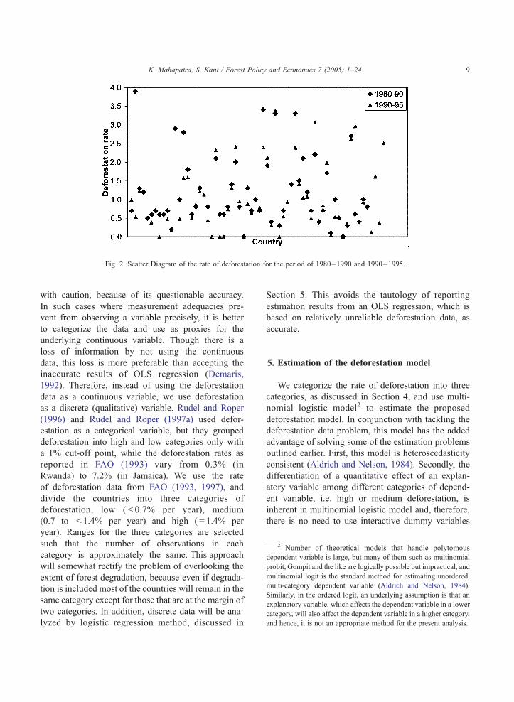
Fig. 2. Scatter Diagram of the rate of deforestation for the period of 1980–1990 and 1990–1995.

2 Number of theoretical models that handle polytomous

dependent variable is large, but many of them such as multinomial

probit, Gompit and the like are logically possible but impractical, and

multinomial logit is the standard method for estimating unordered,

multi-category dependent variable (Aldrich and Nelson, 1984).

Similarly, in the ordered logit, an underlying assumption is that an

explanatory variable, which affects the dependent variable in a lower

category, will also affect the dependent variable in a higher category,

and hence, it is not an appropriate method for the present analysis.

K. Mahapatra, S. Kant / Forest Policy and Economics 7 (2005) 1–24 9

with caution, because of its questionable accuracy.

In such cases where measurement adequacies pre-

vent from observing a variable precisely, it is better

to categorize the data and use as proxies for the

underlying continuous variable. Though there is a

loss of information by not using the continuous

data, this loss is more preferable than accepting the

inaccurate results of OLS regression (Demaris,

1992). Therefore, instead of using the deforestation

data as a continuous variable, we use deforestation

as a discrete (qualitative) variable. Rudel and Roper

(1996) and Rudel and Roper (1997a) used defor-

estation as a categorical variable, but they grouped

deforestation into high and low categories only with

a 1% cut-off point, while the deforestation rates as

reported in FAO (1993) vary from 0.3% (in

Rwanda) to 7.2% (in Jamaica). We use the rate

of deforestation data from FAO (1993, 1997), and

divide the countries into three categories of

deforestation, low ( < 0.7% per year), medium

(0.7 to < 1.4% per year) and high ( = 1.4% per

year). Ranges for the three categories are selected

such that the number of observations in each

category is approximately the same. This approach

will somewhat rectify the problem of overlooking the

extent of forest degradation, because even if degrada-

tion is included most of the countries will remain in the

same category except for those that are at the margin of

two categories. In addition, discrete data will be ana-

lyzed by logistic regression method, discussed in

Section 5. This avoids the tautology of reporting

estimation results from an OLS regression, which is

based on relatively unreliable deforestation data, as

accurate.

5. Estimation of the deforestation model

We categorize the rate of deforestation into three

categories, as discussed in Section 4, and use multi-

nomial logistic model2 to estimate the proposed

deforestation model. In conjunction with tackling the

deforestation data problem, this model has the added

advantage of solving some of the estimation problems

outlined earlier. First, this model is heteroscedasticity

consistent (Aldrich and Nelson, 1984). Secondly, the

differentiation of a quantitative effect of an explan-

atory variable among different categories of depend-

ent variable, i.e. high or medium deforestation, is

inherent in multinomial logistic model and, therefore,

there is no need to use interactive dummy variables

6 There are three types of tests associated with the logistic

regression models. First is the global test for the significance of the

predictor set. The null hypothesis is that all k( j� 1) coefficients

included in the ‘j� 1’ equations are simultaneously zero. The test is

a model chi-squared statistics equal to � 2 log(L0)� [� 2 log(L1)]

with k( j� 1) degrees of freedom, where L0 is the likelihood

function with intercept only, and L1 is the likelihood function with

all the parameter estimates. The second test, the LR test (likelihood

ratio test), is the global test for the impact of one predictor on the

dependent variable in general. The null hypothesis is that all ‘j� 1’

coefficients associated with a particular predictor are simultaneously

zero. In other words, the global test for the variable Xk tests the null

hypothesis that b1k = b2k = ��� = b( j� 1)k = 0. That is, Xk has no effect

on any of the ‘j� 1’ logits. The test is a chi-square test based on the

difference in chi-square statistics between the full model, with all

predictors, and the reduced model, with all predictors except Xk..

The test has ‘j� 1’ degrees of freedom; if it is significant, then Xk

has a significant impact on the endogenous variable. The third test is

K. Mahapatra, S. Kant / Forest Policy and Economics 7 (2005) 1–2410

for categories of deforestation. However, regional

dummy variables will be required to estimate the

effect of regional differences (due to unique character

of a particular region) on deforestation3. Thirdly,

multinomial logistic model is non-linear in nature

(Aldrich and Nelson, 1984). In addition, our theoret-

ical deforestation model is based on underlying causes

of deforestation and, therefore, bias in the parameter

estimation due to simultaneous use of direct and

underlying causes in the same equation is avoided.

The multinomial logistic deforestation model with ‘j’

categories4 of dependent variable can be expressed as:

lnpðcategoryiÞpðcategoryjÞ

" #¼ bi0 þ bi1X1 þ bi2X2

þ : : : þ bi10X10 þ ei ðModel1Þ

Where, j = 3 (High, Medium and Low deforestation);

ith category =High or Medium deforestation; and jth

category = Low deforestation, and X1 to X7 are

explanatory variables as given in the deforestation

model and X8 to X10 are three dummy variables,

IDASIA and IDLAT are regional dummy variables

for countries representing Asia and Latin America,

respectively, and IDPERIOD is the dummy to test

the temporal stability of the model by differentiating

the data between the two periods 1980–1990 and

1990–1995. As there are three categories of the

dependent variable, deforestation, there will be two

non-redundant logits, High/Low and Medium/Low

(hereafter Med/Low)5. For the base line category

(low deforestation), the coefficients are assumed to

be zero (Norusis, 1999).

We also want to examine the suitability of

multinomial logistic method with respect to the

two econometric methods—binary logistics and

ordinary least squares (OLS) method—used in pre-

3 However, we do not include interactive regional dummy

variables due to sample size limitation.4 For j, categories of dependent variable, the jth category is

treated as a baseline category.5 The redundant logit High/Medium is the ratio of High/Low

and Med/Low logits. With some minor calculations, the parameter

estimate of a variable in the High/Medium logit will be the

difference in the parameter estimate of the variable in Med/low

Logit from High/Low logit.

vious studies. Hence, we also estimate the proposed

deforestation model using binary logistic and OLS

methods.

The data on rate of deforestation is divided into

two categories—High and Low for binary logistic.

The cut off point (0.8% rate of deforestation) is

selected so that there are an equal number of obser-

vations in both categories. The mathematical form of

binary logistic deforestation model, as given below, is

same as that of multinomial logistic model, but there

will be only one logit.

lnpðHighÞpðLowÞ

� �¼ bi0 þ bi1X1 þ bi2X2

þ : : : þ bi10X10 þ ei ðModel2Þ

All statistical tests6 and interpretation of results for

binary logistic model are similar to that of multi-

nomial logistic model.

used to determine which logits are significantly affected by Xk. For

large sample sizes, the test that a coefficient is zero can be based on

the Wald statistics, which has a chi-square distribution (Norusis,

1999). A Wald test calculate a Z-statistic which is

Z ¼b j�1ð Þk

S:E: b j�1ð Þk

� �The value is then squared yielding a Wald statistics with chi-square

distribution. The test is based on the null hypothesis that the

coefficient estimate b( j� 1)k is equal to zero in ( j� 1)th logit.

Therefore, the test has 1 (number of restrictions) degree of freedom.

K. Mahapatra, S. Kant / Forest Policy and Economics 7 (2005) 1–24 11

In the case of OLS method, deforestation is treated

as a continuous variable, and the mathematical form

of the model without interactive dummies (as has been

the case in most of the cross-country regression

studies) is given next;

Y ¼ b0 þ b1X1 þ b2X2 þ : : : þ b10X10 þ e

ðModel3Þ

Where, Y is the rate of deforestation, and Xk are the

explanatory variables as in multinomial logistic

model.

However, Model 3 cannot capture the variation in

the effects of the causal variables across different

categories of deforestation, i.e. high and medium.

Therefore, another model (Model 4) that includes all

the variables of Model 3 and interactive dummy

variables for categories of deforestation (the products

of the two dummy variables, HIGH and MED, with

all other explanatory variables such as HIGH*-

POPGR and MED*POPGR) is estimated by OLS

method.7

The coefficient estimate of an explanatory variable

in a given logit, i.e. High/Low, in the multinomial

logistic model, is the difference of coefficients of the

variable in explaining the probability of high defor-

estation (bik) and the probability of low deforestation

(bjk). But, the coefficient estimates of the baseline

category (bjk) are treated as zero (Norusis (1999).

Similarly, the coefficient estimates of the interactive

dummies in OLS model are also the difference in the

effect of variables in a particular category (e.g. High)

from the baseline category (Low).8 Therefore, the

coefficient estimates of a variable in High/Low and

Med/low logits of Model 1 can be interpreted in the

7 In OLS regression the significance of additional variables can

be tested by F-test, which is given as:

F ¼R2new model � R2

old model

� �=df ¼ No: of new regressorsð Þ

1� R2new model

� �df ¼ No:ofparametersinthenew modelð Þ=

8 A significant t-value for a coefficient estimate of an

interactive dummy variable (e.g. HIGH*POPGR) indicates that

the variable (POPGR) has significantly different effect in a

particular category (High) from the baseline category (Low). An

insignificant interactive dummy variable coefficient indicates that it

does not have different effects in different categories.

same way as the coefficient estimates of interactive

dummies for high and medium categories of defor-

estation, respectively.

6. Data and data sources

Our focus is on tropical forests and not on all

categories of woodland. Hence, Forest Resource

Assessment (FRA) dataset of the FAO is the best

available source for deforestation data. As the FRA,

2000 report is not yet widely debated and serious

concerns have been raised about the reported figures

(Matthews, 2001), we preferred to use the compa-

rable dataset of FRA, 1990 (FAO 1993) for the

deforestation data of 1980–1990 period, and SOFO

(State of the World’s forest) 1997 (FAO 1997) for

1990–1995 period. However, the former reports that

the natural forest area is a loss, while the latter

reports that the total forest area (including planta-

tions) is a loss. Hence, the rate of natural forest loss

for the 1990–1995 period is calculated by using the

figures of natural forest area for the year 1995

(SOFO, 1997), the total forest areas in 1990

(SOFO, 1997) and the plantation area in 1990

(FRA 1990).9

Among the independent variables, data on

GDPGR and DEBTGR are calculated. For GDPGR,

time series data from 1980 to 1995 on value added

in agriculture (national currency) is deducted from

the corresponding time series data on GDP (national

currency) at constant prices (1990 = 100). Then two

exponential trend lines are incorporated in the calcu-

lated time series data for 1980–1990 and 1990–

1995 periods, respectively to estimate the average

annual growth rate in GDP excluding the contribu-

tion of agriculture for those periods. Data on total

GDP and value added in agriculture are available in

9 For few countries (Rwanda, Burundi, Kenya, Niger,

Mauritania and India for the for the period 1990–1995), the

calculated rates of loss of natural forest area are negative i.e. an

increase in forest area in 1995. It may be because of an upward

revision of the natural forest area estimates in SOFO 1997 for

those countries. Since, it is unlikely to have increase in natural

forest area in these countries the negative estimates are treated as

zero.

Table 1

Details of the data used for the estimation of deforestation model

Sector Variables Explanation Unit Source

Forest DEF Average annual rate of deforestation Percent FAO, 1993

from 1980–1990 and 1990–1995 FAO, 1997

FORAR Percentage of land area of a country Percent FAO, 1993

under forests in 1980 and 1990 FAO, 1997

Demographic POPGR Average annual growth rate of Percent FAO, 1993

population from 1980–1990 and 1990–1995 FAO, 1997

Macro-economic GDPGR* Average annual growth rate of GDP Percent World Bank, 1999

(excluding agriculture) during 1980–1990 and 1990–1995

DEBTGR* Average annual growth rate of Total Debt Percent World Bank, 1999

service as a percentage of GNP during

1980–1990 and 1990–1995

Agriculture AGGR Average annual growth rate of agricultural Percent World Bank, 1997

sector during 1980–1990 and 1990–1995

Infrastructure ROAD Percentage paved road of a country Percent World Bank, 1999

for the years 1990 and 1995

Political DEMOCRACY Average DEMOCRACY index of a country Integer Gurr and Jaggers, 1999

during 1980–1990 and 1990–1995

Note: *Values of these variables are calculated.

11 Countries included in the final analysis are: Angola,

Bangladesh, Benin, Bhutan, Bolivia, Botswana, Brazil, Burkina

Faso, Burundi, Cambodia, Cameroon, Central African Republic,

Chad, Colombia, Congo, Costa Rica, Cote d’Ivoire, Dominican

Republic, Ecuador, El Salvador, Gabon, Gambia, Ghana, Guate-

mala, Guinea, Guinea-Bissau, Guyana, Haiti, Honduras, India,

K. Mahapatra, S. Kant / Forest Policy and Economics 7 (2005) 1–2412

World Bank (1999). Similarly, DEBTGR for differ-

ent countries for the periods 1980–1990 and 1990–

1995 are calculated by incorporating exponential

trend lines in the available time series data for those

periods.

The data for paved roads is not available for the

period of 1980–1990.10 Hence, the effect of road as a

level (ROAD) vis-a-vis growth variable (ROADGR)

will be tested for the period 1990–1995 for which

time series data is available. If results of the variable

in both forms will be similar, road as a level variable

will be used as a proxy for road as growth variable in

the final model.

We began our preliminary analysis with 90 tropical

countries included in the FRA 1990. However, due to

non-availability of data on some of the explanatory

variables for 26 countries, only 64 countries, compris-

ing of 33 African, 13 Asian and 18 Latin American

countries, are included in the final analysis. Data for

these countries are collected for the periods 1980–

10 Average annual change in each variable for two different

periods, i.e., 1980–1990 and 1990–1995 are used in the model.

Therefore, for each country there will be two observations. For

the ROAD variable, data prior to 1990 are not available.

Therefore, percentage paved road in a country during 1990 and

1995 will be used as ROAD variable for two periods,

respectively.

1990 and 1990–1995, but for some countries, data for

all the variables are not available for both the periods,

which reduced the number of effective observations to

117.11 The list of all the variables with their explan-

ations, units of measurement and sources are given in

Table 1 and descriptive statistics in Table 2.

7. Comparative discussion of results from three

econometric methods

First, the effects of road on deforestation as a

growth variable (ROADGR) and as a level variable

Indonesia, Kenya, Liberia, Madagascar, Malawi, Malaysia, Mali,

Mauritania, Mexico, Mozambique, Nepal, Nicaragua, Niger,

Nigeria, Pakistan, Panama, Papua New Guinea, Paraguay, Peru,

Philippines, Rwanda, Senegal, Sierra Leone, Somalia, Sri-Lanka,

Tanzania, Thailand, Togo, Trinidad and Tobago, Uganda, Ven-

ezuela, Vietnam, Zambia and Zimbabwe. For the period of 1980–

1990, Guinea, Tanzania, Bhutan, Cambodia, Vietnam, Haiti and

Nicaragua, and for the period 1990–1995, Liberia, Somalia, Sri

Lanka and Bolivia are excluded.

Table 2

Descriptive statistics for the variables of the deforestation model (N= 117)

DEF FORAR POPGR GDPGR DEBTGR AGGR ROAD DEMOCRACY

Mean 1.11 33.85 2.65 2.77 1.82 2.34 21.38 3.47

Min. 0.00 0.47 0.90 �12.95 �55.11 �10.80 0.17 0.00

Max. 3.90 95.48 4.20 10.29 37.45 12.20 75.00 10.00

S.D. 0.91 21.84 0.65 3.65 12.47 2.89 15.77 3.55

K. Mahapatra, S. Kant / Forest Policy and Economics 7 (2005) 1–24 13

(ROAD) are compared. Since, the data on

ROADGR is available only for 1990–1995 period,

two multinomial logistic regressions were estimated

for this period by including ROAD and ROADGR

variables, respectively, along with all other explan-

atory variables. The results of LR test indicate that

ROAD is significant at a 10% level of signifi-

cance,12 but ROADGR is not. The results of the

Wald test indicate that ROAD is significant, at 10%

level, in one of the logits (Med/Low), but

ROADGR is not significant in any of the logits.

Nevertheless, the signs of coefficients are positive

for both variables. The variation in significance

could be due to insufficient degrees of freedom

(N�K = 46) of the model. The direction of causal

effect of road being the same when used as a

growth or level variable, the level variable (ROAD)

is used for the full model (for the combined periods

of 1980–1990 and 1990–1995).

Second, temporal stability was tested for all

four models, i.e. multinomial, binary, and two

models of OLS, by estimating these models

including the dummy variable IDPERIOD. The

results of LR and Wald tests for multinomial and

binomial models and t-test13 for OLS models

12 A 10% level of significance is selected to test the

significance of the results. Bendel and Afifi (1977) quoted in

Menard (1995) even pointed out that it is beneficial to accept a 15 to

20 % of level of significance, which increases the risk of rejecting

the null hypothesis when it is true (finding a relationship that is not

really there), but decreases the risk of failing to reject the null

hypothesis when it is false (not finding a relationship that is really

there).13 At 5% level of significance, heteroscedasticity was found

in all the OLS regressions. The t-statistics of different variables

are the consistent t-values after White’s correction for hetero-

scedasticity.

indicate that the dummy variable (IDPERIOD) is

not significant in any of the models. This suggests

that there is temporal stability in the relationship

between deforestation and its causal factors. Hence,

the dummy variable IDPERIOD is dropped and all

models are estimated again with the full set of

data, 117 observations (N = 117 in all succeeding

models), and results are discussed in the following

sections.

7.1. Multinomial logistic model (Model 1)

The results of the model are given in Table 3. The

chi-square statistics for the overall model (calculated

value 71.036>critical value of 25.989 for 18 degrees

of freedom and 10% significance-level) indicates that

the model is significant. The LR test for significance

of a predictor shows that all variables except GDPGR

and DEMOCRACYare significant at 10% level in the

overall model. The Wald test for significance of

coefficient estimates in different logit suggests that

the variables FORAR, POPGR, AGGR, ROAD, IDA-

SIA and IDLAT are significant at 10% significance

level in High/Low logit, while DEBTGR, AGGR,

ROAD and IDASIA variables are significant in

Med/low logit.

7.2. Multinomial logistic model (Model 1) vs. binary

logistic model (Model 2)

Similar to multinomial logistic model, the overall

binary logistic model is also significant at a 10%

significance level (calculated chi-square statistics

51.194>the critical chi-square value of 14.683, for

nine degrees of freedom and 10% significance level).

Results of LR test indicate that all variables have a

similar pattern of significance in both the models,

except for DEBTGR, which is significant in multi-

Table 3

Results of multinomial logistic regression (N= 117)

Variable Likelihood Wald test

Ratio testHigh/Low Med/Low

Chi-squareb Wald Exp (b) b Wald Exp ()

INTERCEPT 13.592* �6.670 10.695* �4.084 4.893*

FORAR 4.315+ �0.0299 3.696* 0.971 �0.00375 0.082 0.996

POPGR 7.116* 1.420 6.194* 4.138 0.791 2.345 2.206

GDPGR 2.660 �0.178 2.016 0.837 0.02285 0.055 1.023

DEBTGR 7.564* 0.01199 0.212 1.012 0.06147 6.508* 1.063

AGGR 7.801* 0.263 2.855* 1.301 0.311 5.947* 1.365

ROAD 7.991* 0.04206 4.348* 1.043 0.05161 5.848* 1.053

DEMOCRACY 1.085 0.03812 0.146 1.039 0.09467 1.055 1.099

IDASIA 25.352* 3.745 10.298* 42.326 �2.039 2.907* 0.130

IDLAT 29.171* 4.511 16.522* 91.018 0.08741 0.008 1.091

Note: *Significant at 10% level of significance. The critical values at 10% level of significance are 2.705 for 1 degree of freedom (Wald test)

and 4.605 for 2 degrees of freedom (LR test).+Significant at 11.6% level of significance (significance of this result is discussed in Section 8).

K. Mahapatra, S. Kant / Forest Policy and Economics 7 (2005) 1–2414

nomial logistic, but not in binary logistic. The signs of

the coefficients and the results of the Wald test for the

significance of different predictors in High/Low and

Med/Low logits of multinomial logistic model, and

the High/Low logit of binary logistic model are

presented in Table 4.

The signs of all variables in High/Low logit of

multinomial logistic are the same as in High/Low logit

of binary logistic. But, the signs of variables GDPGR

and IDASIA in Med/Low logit of multinomial logistic

are opposite to the signs of these variables in a single

Table 4

Signs and significance of parameter estimates in multinomial and binary

Variable Multinomial logistic

High/Low

FORAR �Sig. (0.055)

POPGR +Sig. (0.013)

GDPGR �N.S. (0.156)

DEBTGR +N.S. (0.645)

AGGR +Sig. (0.091)

ROAD +Sig. (0.037)

DEMOCRACY +N.S. (0.703)

IDASIA +Sig. (0.001)

IDLAT +Sig. (0.000)

Note: Values in brackets are the P-values for the parameter estimates.

Sig. means significant and N.S. means not significant at 10% level of sig

High/Low logit of binary logistic model. The varia-

bles AGGR, ROAD and IDASIA are significant and

the variables GDPGR and DEMOCRACY are insig-

nificant in binary and both logits of multinomial

logistic model. POPGR is significant in binary logistic

indicating that it is a causal factor of deforestation in

high deforesting countries. However, the POPGR

variable is significant only in one logit—High/

Low—of the multinomial logistic regression. This

suggests that POPGR is the causal factor for a group

of countries and not for all those countries that were

logistic models (N = 117)

Binary logistic

Med/Low High/Low

�N.S. (0.774) �N.S. (0.274)

+N.S. (0.126) +Sig. (0.000)

+N.S. (0.815) �N.S. (0.115)

+Sig. (0.011) +N.S. (0.350)

+Sig. (0.015) +Sig. (0.020)

+Sig. (0.016) +Sig. (0.004)

+N.S. (0.304) +N.S. (0.973)

�Sig. (0.088) +Sig. (0.001)

+N.S. (0.927) +Sig. (0.001)

nificance.

Table 5

Sign and significance of parameter estimates in multinomial logistic and OLS regression without interactive dummies (N = 117)

Variable Multinomial logistic OLS (without

High/Low Med/Lowinteractive dummies)

FORAR �Sig. (0.055) �N.S. (0.774) �Sig. (1.75)

POPGR +Sig. (0.013) +N.S. (0.126) +Sig. (3.50)

GDPGR �N.S. (0.156) +N.S. (0.815) �N.S. (0.44)

DEBTGR +N.S. (0.645) +Sig. (0.011) +N.S. (1.28)

AGGR +Sig. (0.091) +Sig. (0.015) +N.S. (1.48)

ROAD +Sig. (0.037) +Sig. (0.016) +N.S. (0.56)

DEMOCRACY +N.S. (0.703) +N.S. (0.304) �N.S. (0.03)

IDASIA +Sig. (0.001) �Sig. (0.088) +Sig. (3.46)

IDLAT +Sig. (0.000) +N.S. (0.927) +Sig. (5.93)

Note: For multinomial logistic model numbers in brackets are the P-values for the parameter estimates, and for OLS model the numbers are the

t-values.

Sig. means significant and N.S. means not significant at 10% level of significance. The critical t-value (for t-test in OLS regression) at 10% level

of significance is 1.671 for 60 degrees of freedom and 1.658 for 120 degrees of freedom. In our case, the OLS regression has 108 (N�K=108)

degrees of freedom.

K. Mahapatra, S. Kant / Forest Policy and Economics 7 (2005) 1–24 15

treated as high category in binary logistic regres-

sion.14 The significance pattern of IDLAT is the same

as that of POPGR. The significance of the IDLAT

variable in High/Low logit of binary logistic regres-

sion indicates that Latin American countries have a

greater probability of having high deforestation than

the African countries (base category). The insignif-

icant coefficient of IDLAT in Med/Low logit of

multinomial logistic regression, however, suggests

that not all countries that were included in the high

deforesting category in binary logistic model have a

greater probability of high deforestation. Similarly,

DEBTGR is significant in Med/Low logit of multi-

nomial logistic model, but not in binary logistic. That

is, debt service is a significant factor of deforestation

in medium deforesting countries, which otherwise is

not decipherable from the binary logistic model.

These differences clearly demonstrate that the varia-

tion in the signs and significance of variables across

three categories (high, medium and low deforestation)

of countries is suppressed in binary logistic model,

14 In binary logistic model, the countries of medium

category from multinomial logistic model are redistributed among

the high and low categories. POPGR does not have any effect in

those countries of the high category in binary logistic regression

that are treated as medium category in multinomial logistic

regression.

and multinomial logistic regression should be used to

capture that.

7.3. Multinomial logistic model vs. OLS regression

models (Model 3 and 4)

The OLS model without interactive dummy varia-

bles15 (Model 3) is significant at 1% significance level

(F-value of 5.80 at 9, 107 degrees of freedom).

Results of signs and significance of parameter esti-

mates, however, indicate how best a model is infor-

mative. Table 5 presents sign and significance of the

parameter estimates in multinomial logistic and OLS

model without interactive dummies. A comparison

between multinomial logistic with that of OLS model

without interactive dummies shows that all the vari-

ables have same sign pattern except GDPGR,

DEMOCRACY and IDASIA. The signs of GDPGR

and IDASIA variables in OLS model are at least

similar to the sign of these variables in High/Low

logit. However, the sign of DEMOCRACYvariable in

OLS model is different from those in two logits. Tests

of significance for those variables, for which the sign

pattern is the same, indicate that while AGGR and

ROAD are significant in both logits, they are not in

OLS model. Similarly, DEBTGR is significant in at

15 Diagnostic tests (eigen values and conditioning index) show

absence of multi-collinearity in all OLS regressions.

K. Mahapatra, S. Kant / Forest Policy and Economics 7 (2005) 1–2416

least one logit, but not in OLS model. While POPGR

and FORAR are significant in OLS model, it is true

for only one logit (High/Low). It is possible that the

variation in sign and significance of the variables in

the OLS model from the multinomial logistic model

are due to exclusion of interactive dummies in OLS

model. Therefore, the OLS model is re-estimated after

including the interactive dummies, as explained in

Section 5.

Model 4 (OLS with interactive dummies) is sig-

nificant at 1% level of significance (F-value of 27.92

at 29, 87 degrees of freedom). The F-test for the

significance of the additional variables shows that

they have significant effect on the dependent variable.

The sign and significance of the variables in multi-

nomial logistic and Model 4 are given in Table 6. A

comparison of coefficient signs of variables in High/

Low logit with those of the interactive dummy vari-

ables of high deforestation category in OLS indicate

that FORAR, POPGR, DEBTGR, IDASIA and

IDLAT variables have the same sign pattern in the

two models. However, other variables have opposite

signs. The tests of significance for variables for which

the sign patterns are same indicate that the variable

POPGR is significant in High/Low logit, but not

significant at 10% level of significance in OLS model.

Similarly, a comparison between the coefficient signs

of variables in Med/Low logit and the interactive

dummy variables of medium deforestation category

Table 6

Sign and significance of parameter estimates in multinomial logistic and

Variable Multinomial logistic

High/Low Med/Low

FORAR �Sig. (0.055) �N.S. (0.774)

POPGR +Sig. (0.013) +N.S. (0.126)

GDPGR �N.S. (0.156) +N.S. (0.815)

DEBTGR +N.S. (0.645) +Sig. (0.011)

AGGR +Sig. (0.091) +Sig. (0.015)

ROAD +Sig. (0.037) +Sig. (0.016)

DEMOCRACY +N.S. (0.703) +N.S. (0.304)

IDASIA +Sig. (0.001) �Sig. (0.088)

IDLAT +Sig. (0.000) +N.S. (0.927)

Note: For multinomial logistic model numbers in brackets are the P-values

t-values.

Sig. means significant and N.S. means not significant at 10% level of sign

60 degrees of freedom and 1.658 for 120 degrees of freedom. In our case

Dummy for High describes the HIGH*explanatory variables and dummy

in Model 4 indicate that POPGR, AGGR, ROAD and

IDLAT have similar signs, while for other variables

the signs are different in the two models. The tests of

significance of the variables, for which the sign

pattern is the same, indicate that AGGR and ROAD

variables are significant in Med/Low logit, but not the

corresponding variables in OLS regression.

Maximum–Likelihood (ML) estimation procedure,

which is used to estimate the logistic regression

models, is a visible alternative to OLS in nearly all

situations to which the latter applies. Asymptotically

(for a sample size of around N�K = 100) the ML

estimates exhibit the properties of unbiasedness, effi-

ciency and normality, similar to that of OLS estimates

(Aldrich and Nelson, 1984). In these circumstances, it

is not possible to argue superiority of one model (say

multinomial logit) over the other model (OLS with

interactive dummy variables). However, stability of

results with respect to variation in deforestation data

may provide an important guiding factor for the

preference of one of these models.

7.4. Stability of the results of multinomial logistic

model and OLS model with interactive dummy

variables

The basic reason behind using deforestation as a

qualitative variable is the questionable accuracy of

deforestation data. Hence, we test the stability of the

OLS regression with interactive dummies (N=117)

OLS (with interactive dummies)

Dummy for High Dummy for Medium

�Sig. (3.80) +N.S. (1.15)

+N.S. (1.11) +N.S. (1.61)

+N.S. (1.23) �N.S. (0.99)

+N.S. (1.02) �N.S. (0.37)

�Sig. (2.10) +N.S. (0.13)

�Sig. (2.72) +N.S. (0.63)

�N.S. (1.06) �N.S. (0.54)

+Sig. (3.20) +N.S. (1.23)

+Sig. (2.24) +Sig. (2.20)

for the parameter estimates, and for OLS model the numbers are the

ificance. The critical t-value at 10% level of significance is 1.671 for

, the OLS regression has 88 (N�K=88) degrees of freedom.

for Medium describes MED*explanatory variables.

Table 7

Sign and significance of parameter estimates in OLS with interactive dummies after random changes in the rates of deforestation (N=117)

Variable Before change in rate of deforestation After change in rate of deforestation

Base Dummy for Dummy for Base Dummy for Dummy for

category High Medium category High Medium

INTERCEPT +N.S. (0.10) +Sig. (3.30) +N.S. (0.09) +N.S. (0.22) +Sig. (3.23) - N.S. .(0.07)

FORAR +Sig. (2.10) �Sig. (3.80) +N.S.(1.15) +Sig. (2.44) �Sig. (3.96) + N.S. (0.97)

POPGR +N.S. (1.07) +N.S. (1.11) +N.S. (1.61) +N.S. (0.97) +N.S. (1.15) + Sig. (1.69)

GDPGR +N.S. (1.11) +N.S. (1.23) �N.S. (0.99) +Sig. (1.65) +N.S. (1.15) - N.S.(1.39)

DEBTGR �N.S. (0.25) +N.S. (1.02) �N.S.(0.37) �N.S. (0.25) +N.S. (1.26) + N.S. (0.07)

AGGR +N.S. (0.23) �Sig.(2.10) +N.S. (0.13) �N.S. (0.25) �Sig. (1.90) + N.S. (0.40)

ROAD +N.S. (0.69) �Sig. (2.72) +N.S. (0.63) +N.S. 0.38) �Sig. (2.46) + N.S. (0.95)

DEMOCRACY +N.S. (0.14) �N.S. (1.06) �N.S.(0.54) �N.S.(0.54) �N.S. (0.83) - N.S. (0.09)

IDASIA �N.S. (0.93) +Sig. (3.20) +N.S(1.23) �N.S. (1.44) +Sig. (3.33) + Sig. (1.63)

IDLAT �N.S.(1.02) +Sig. (2.24) +Sig.(2.20) �N.S. (1.16) +Sig. (2.37) + Sig. (2.34)

Note: The numbers in the brackets are the t-values.

Sig. means significant and N.S. means not significant at 10% level of significance. The critical t-value at 10% level of significance is 1.671 for

60 degrees of freedom and 1.658 for 120 degrees of freedom. In our case, the OLS regression has 88 (N�K=88) degrees of freedom.

K. Mahapatra, S. Kant / Forest Policy and Economics 7 (2005) 1–24 17

results of multinomial logistic and OLS models for

variations in deforestation data. First the stability of

OLS results is tested by random variation in defores-

tation data (as a continuous variable). Second, the

stability of multinomial logistic regression results is

tested by varying the cutoff points for three categories

(High, Medium and Low) of deforestation. A common

understanding is that deforestation data is under

reported by national agencies. Hence, the rates of

deforestation for different countries are increased ran-

domly by 0 to 7%,16 and the multinomial logistic

model and OLS model with interactive dummies are

re-estimated.17 Since the qualitative categorization of

countries remains unchanged, results from multino-

mial logistic are the same as before, but the sign and

significance of the variables in the OLS model are

changed. Table 7 gives the comparative picture of the

sign and significance of the variables for OLS models,

both before and after changes in the rates of defores-

tation. The signs of coefficient estimates of the varia-

16 The upper limit of the change in deforestation (7%) is

selected such that there is no change in the categorization of

countries in three categories (High, Medium, and Low) of

deforestation.17 Random numbers, from 1 to 7, are generated for all 117

observations, and deforestation rate is increased by respective

random percentage point for each observation. Random numbers are

generated four times and hence, deforestation rates are varied for

four times. The results with respect to sign and significance of the

variables remained same every time.

bles DEBTGR (in medium deforestation category),

AGGR (base category) and DEMOCRACY (base

category) have changed in the re-estimated OLS

model. In addition, the variables POPGR and IDASIA

in medium deforestation category become significant

while they were not in the original OLS model. These

results indicate that results of OLS regression are not

stable with respect to change in deforestation data.

The stability of multinomial regression is tested by

changing (decreasing and increasing) the cut-off

points by 7%, (the same rate by which the rates of

deforestation are changed in the OLS model), and re-

estimating the multinomial logistic model18. A com-

parative picture of the signs and significance of

coefficient is given in Table 8. The results reveal that

the signs and significance remain unchanged for a 7%

decrease in the cut-off points, and the signs and

significance are almost the same as that of the original

model for a 7% increase in the cut off points with two

exceptions. The POPGR variable, which is insignif-

18 The lower cut-off point in medium category of deforestation

is 0.7% per year, and in high deforestation category it is 1.4% per

year. The number of observations in low category is 44, in medium

40, and in high 33. After 7% decrease, the cut-off points for medium

and high categories are 0.651and 1.302, respectively, and the

number of observations are 43, 40 and 34 for low, medium and high

categories, respectively. Similarly, after 7% increase, the new cut-off

points are 0.749 and 1.498 for medium and high categories,

respectively, and number of observation are 54, 33 and 30 in low,

medium and high deforestation categories, respectively.

Table 8

Sign and significance of coefficient estimates in original multinomial logistic regression model vs. those from new models after change in the

cut-off points (N=117)

Variable Original model After 7% decrease in the After 7% increase in the

cut-off points cut-off points

High/Low Med/Low High/Low Med/Low High/Low Med/Low

FORAR �Sig. (0.055) �N.S. (0.774) �Sig. (0.066) �N.S. (0.721) �Sig. (0.089) �N.S. (0.565)

POPGR +Sig. (0.013) +N.S. (0.126) +Sig. (0.009) +N.S. (0.153) +Sig. (0.002) +Sig. (0.004)

GDPGR �N.S. (0.156) +N.S. (0.815) �N.S. (0.157) +N.S. (0.781) �N.S. (0.187) +N.S. (0.121)

DEBTGR +N.S. (0.645) +Sig. (0.011) +N.S. (0.638) +Sig. (0.010) +N.S. (0.505) +Sig. (0.079)

AGGR +Sig. (0.091) +Sig. (0.015) +Sig. (0.098) +Sig. (0.014) +N.S. (0.126) +Sig. (0.008)

ROAD +Sig. (0.037) +Sig. (0.016) +Sig. (0.032) +Sig. (0.017) +Sig. (0.039) +Sig. (0.003)

DEMOCRACY +N.S. (0.703) +N.S. (0.304) +N.S. (0.622) +N.S. (0.337) +N.S. (0.774) +N.S. (0.421)

IDASIA +Sig. (0.001) �Sig.(0.088) +Sig. (0.002) �Sig. (0.093) +Sig. (0.000) +N.S. (0.838)

IDLAT +Sig. (0.000) +N.S. (0.927) +Sig. (0.000) +N.S. (0.876) +Sig. (0.000) +N.S. (0.223)

Note: Numbers in brackets are the P-values for the parameter estimates.

Sig. means significant and N.S. means not significant at 10% level of significance.

K. Mahapatra, S. Kant / Forest Policy and Economics 7 (2005) 1–2418

icant in Med/Low logit of the original model,

becomes significant in the new model. Similarly, the

coefficient estimate of the IDASIA variable is signifi-

cant and has a negative sign in the Med/Low logit of

the original model; but the coefficient estimate

becomes positive, though insignificant in the new

model. These variations could be due to major

changes in the number of observations in the low

(from 44 to 54) and medium (from 40 to 33) defor-

estation categories. Hence, the results of multinomial

logistic model are relatively stable compared to OLS

model, and less subject to changes due to deforesta-

tion data problems. Therefore, the results of multi-

nomial logistic model are discussed next in detail.

8. Discussion of results from multinomial logistic

model

The results of multinomial logistic model are given

in Table 3, and some aspects were discussed in

Section 7.1. One interesting feature of these results

is that the variable FORAR though not significant in

the Likelihood Ratio test, is significant in Wald test19

19 There are some disadvantages of using Wald test over

Likelihood Ratio test. For large coefficients, the estimated standard

error becomes too large resulting in failure to reject the null

hypothesis that the coefficient is zero, when in fact it should not be.

This means a variable significant in Likelihood Ratio test might not

be in case of Wald test (Menard, 1995; Norusis, 1999). But, in our

case the results are reverse.

for High/Low logit. But, the significance level in

Likelihood Ratio test is at 11.6%, which is not far

away from the 10% level of significance that we

have chosen for our analysis. Therefore, the effect

of the variable FORAR is considered as significant,

at least in the High/Low logit. Based on the

results, the equations for the two non-redundant

logits, High/Low (L1) and Med/Low (L2), are given

below:

L1 ¼ lnp Highð Þp Lowð Þ

� �¼ �6:670� 0:0299*FORAR

þ 1:420*POPGR

� 0:178*GDPGR

þ 0:01199*DEBTGR

þ 0:263*AGGR

þ 0:04206*ROAD

þ 0:03812*DEMOCRACY

þ 3:745*IDASIA

þ 4:511*IDLAT

p Medð Þ� �

2 ¼ lnp Lowð Þ ¼ �4:086� 0:00375*FORAR

þ 0:791*POPGR

L

þ 0:02285*GDPGR

þ 0:06147*DEBTGR

þ 0:311*AGGR

þ 0:05161*ROAD

þ 0:09467*DEMOCRACY

� 2:039*IDASIA

þ 0:08741*IDLAT

K. Mahapatra, S. Kant / Forest Policy and Economics 7 (2005) 1–24 19

The coefficients of explanatory variables in these

equations can be interpreted as the change in the

log odds associated with a one-unit change in the

explanatory variable. A positive or negative coef-

ficient of a variable increases or decreases the log

odds, when other predictors are constant. For

example, the coefficient of 1.420 for POPGR, in

High/Low logit, suggests that when population

growth changes by one unit (1% per year), the

values of other variables remaining the same, the

log odds of a country being in the category of

high deforestation increase by a factor of 1.420.

However, it is easier to think of odds rather than

log odds in interpreting the parameter estimates.

The base of natural logarithm (approximately

2.718) raised to the power equal to the magnitude

of the coefficient denotes the factor by which the

odds (rather than log odds) change when the

independent variable increases by one unit. For

example, in High/Low logit, when population

growth increases by 1%, the odds in favor of a

country being in high deforestation increase by a

factor of 4.138 (e1.420). Similar is the case for

other variables, which are given in the column of

Exp (h) of Table 3. These results with respect to

each variable are discussed in the following para-

graphs.

The coefficient of FORAR has a negative sign in

both logits, but it is significant in the High/Low logit

and insignificant in the Med/Low logit. Hence, in high

deforestation countries the effect of per unit forest

area pressure dominates the effect of free common

good attitude, and the odds in favor of high defor-

estation decreases by a factor of 0.971 with 1% rise in

the percentage of land area under forests. However, in

medium deforestation countries, the effect of per unit

forest area pressure is somewhat neutralized by the

effect of free common good attitude and therefore, the

parameter estimate is negative, but not significant.

The odds in favor of medium deforestation remain

almost constant (a factor of 0.996) with 1% increase

in the percentage of land area under forests.

Population growth (POPGR) has a positive sign in

both the logits, but it is significant in High/Low logit

and insignificant in Med/Low logit. Results suggest

that an increase in population growth by 1% increases

the likelihood by a factor of 4.138 of a country being

in high deforestation category than in low deforesta-

tion. This result strengthens the dominance of Mal-

thusian proposition over the Boserup proposition and

out-migration phenomenon in high deforestation

countries. The positive and insignificant parameter

estimate in Med/Low logit denotes that population

growth increases the likelihood of a country being in

medium category than in low deforestation category,

but not significantly. The odds in favor of medium

deforestation increase by a factor of 2.206 with 1%

rise in the rate of population growth. This indicates

the stronger effects of Boserup hypothesis and out-

migration phenomenon, which neutralizes the Mal-

thusian effect, in medium deforestation countries as

compared to high deforestation countries. Since the

significance level of this parameter estimate is at

12.6% against the chosen 10%, it cannot be ruled

out that with rise in population, the harmful effects on

deforestation will dominate the neutralizing effects,

and therefore, deforestation.

The coefficient of GDPGR is negative in High/

Low logit, and positive in Med/Low logit, but insig-

nificant in both logits. These opposite signs indicate

that an increase in economic growth decreases the

probability of a country being in the category of high

deforestation, but increases the probability of a coun-

try being in medium deforestation category. This

means, the beneficial effects of economic growth on

deforestation are greater, but somewhat neutralized by

the detrimental effects in high deforestation countries,

while detrimental effects are stronger than the bene-

ficial effects in medium deforestation countries. One

possible explanation for this phenomenon can be

provided by the percolation of beneficial effects of

economic growth. It seems that in high deforesting

countries, people with low level of income reap some

of the benefits of economic growth and involve

themselves with environment friendly activities away

K. Mahapatra, S. Kant / Forest Policy and Economics 7 (2005) 1–2420

from forests. However, in medium deforesting coun-

tries, the benefits may be concentrated in the hands of

wealthy people, and the poor farmers continue to

contribute to forest destruction.

The coefficient of debt service (DEBTGR) is

positive in both logits, but significant in Med/Low

logit and insignificant in High/Low logit. This

means that the contributions of forest sector to debt

service are dominating over the contributions of

debt to reduce the pressure on forests in medium

deforestation countries, while in high deforestation

countries these two effects are almost neutralized.

Statistics on forest products trade (FAO, 1997; page

63 and 192–195) somewhat corroborate these

results. Tropical Latin American countries in general

are both exporters as well as importers with former

greater than the latter. Export of forest products is

quite higher than import in almost all tropical

African countries except some in West Sahelian

Africa (Mauritania, Niger, Senegal). Majority of

tropical Asian countries import a substantial amount

of forest products except for Malaysia and Indone-

sia. Most of the high deforesting countries are from

Latin America with fewer representations from Asia

and Africa, where forest product export is slightly

greater than import. In fact some of the countries

are involved in the business of importing from one

country and exporting to another without doing any

harm to their own forest resource. Therefore, the

effect on deforestation in these countries is not

significant. Most of the countries in medium defor-

estation category, however, are from Africa where

export is far higher than import. Therefore, the

effect of debt service is significant in this category.

These countries are the poorest in the world with

debt piling on every year. With no other alternatives

available, they use forest product export as a means

of meeting their debt obligation.

The coefficients of agriculture growth (AGGR)

and road (ROAD) variables are positive and signifi-

cant in both the logits. The effects of both variables

are similar in both categories of deforestation. With

1% rise in agricultural growth, the likelihood of a

country being in the category of high deforestation

increases by a factor of 1.301, and being in medium

deforestation by a factor of 1.365. Similarly, the

odds in favor of high and medium deforestation

increase by a factor of 1.043 and 1.053, respec-

tively, for a 1% rise in length of paved road. Hence,

in both categories of countries, the expansion effect

of agricultural growth is dominating over its inten-

sification effect, and accessibility effect of roads, for

logging and encroachment, is dominating over better

management effect.

The coefficients level of democracy (DEMOC-

RACY) variable are positive, but insignificant in both

the logits. These results contradict the results reported

by Didia (1997) and Deacon (1994), who concluded

that democratic societies would be having low defor-

estation. Countries such as Ecuador, Trinidad and

Tobago, Nicaragua, Costa Rica and Thailand are

democratic in nature, but have high deforestation,

while most of the African countries considered

undemocratic such as Burundi, Cameroon, Congo,

Somalia and Rwanda have low deforestation rate.

These results support an argument that democracy

does not have any significant effect on forest

conservation.

The coefficient estimates of IDASIA and IDLAT

variables are positive and significant in High/Low

logit. This means, being in Latin America or Asia

rather than in Africa increases the probability of

observing a country in the category of high defores-

tation with respect to low deforestation. The high EXP

(b) values of IDASIA and IDLAT variables denotes

that apart form the variables included in the model,

there are some other causal variables that cause high

deforestation in Asian and Latin American countries.

The coefficient of IDASIA is negative and significant

in Med/Low logit, implying that a country being in

Asia (rather than in Africa) increases the likelihood of

low deforestation. The coefficient of IDLAT has a

positive sign, but insignificant in Med/Low logit

suggesting that being in Latin America does not

increase the likelihood of observing a country having

medium deforestation.

9. Country-specific policy priorities

The results obtained from the previous analyses

can be further refined to find and prioritize the

country-specific importance of causal variables of

deforestation, so that country-specific policy interven-

tions can be suggested. For illustration, we selected

five countries each, for which the predicted probabi-

Table 9

Percentage change in probabilities of various countries being in high or medium deforestation categories with a 10% ceteris paribus increase in

causal variables

FORAR POPGR GDPGR DEBTGR AGGR ROAD DEMOCRACY

High

Ecuador �4.16 6.60 �0.86 �0.06 0.37 0.14 �0.83

Guatemala �3.35 5.90 �0.33 �0.86 0.22 0.27 �0.17

Honduras �3.54 6.32 �1.33 �0.04 0.18 0.15 �0.51

Pakistan �0.06 1.87 �0.91 �0.14 0.06 0.05 �0.26

Paraguay �3.15 6.78 �1.06 �0.70 0.58 0.20 �0.03

Medium

Benin 0.04 1.92 0.23 0.50 1.58 1.10 0.98

Gambia 0.02 2.46 0.41 1.46 0.18 2.29 1.11

Madagascar 0.15 2.45 0.06 1.67 1.19 1.22 1.42

Mali 0.08 2.66 0.37 1.68 1.68 1.10 1.33

Nigeria 0.08 2.36 0.10 1.77 1.76 2.63 0.44

K. Mahapatra, S. Kant / Forest Policy and Economics 7 (2005) 1–24 21

lities20 are highest in the observed category, from high

and medium deforestation categories. For all selected

10 countries, a 10% increase from the current level is

made in each causal variable, and the respective

predicted probabilities and the percentage changes in

predicted probabilities with respect to the ceteris

paribus, a 10% change in each variable are estimated

for the period of 1990–1995. The variable that

changes the probability the most is the number one

causal factor to be addressed, followed by the factor

that makes the second highest change in the proba-

bility. Table 9 outlines such changes in predicted

probabilities for all the 10 selected countries.21

20 Predicted probabilities for each country to be in high,

medium and low category are calculated by the formula pi ¼eLi

1þPj�1

i¼1

eLi

Where, i = 1,2 =High and Medium deforestation and j = 3

(total number of categories of dependent variable). A country is

classified to a particular category of deforestation for which the

estimated probability is the highest. The predicted categorization is

then compared with the observed categorization.21 The predicted probability for high and medium category

changes in a direction according to the coefficient sign of the variable

in L1 and L2, respectively. For instance, an increase in GDPGR

decreases/increases the predicted probability of high/medium

deforestation as it has a negative and positive sign in L1 and L2respectively. However, when the coefficient estimate has same sign

in both the logits the change in the predicted probability for a

category depends on the numeric values of the coefficient estimate in

L1 and L2. For example, DEBTGR has positive sign in both L1 and

L2, but the coefficient estimate in L2 has a higher numeric value than

in L1. Therefore, changes in the probability of high deforestation will

be in the opposite direction of the changes in DEBTGR. Similar is

the case for DEMOCRACY in the high deforestation category and

FORAR in the medium deforestation category.

In 1990–1995 period, for example, Pakistan is in

the high deforestation category and the predicted

probability of high deforestation is 0.908. A ceteris

paribus 10% rise in POPGR from the current level

(i.e. from 2.80 to 3.08) results in a predicted proba-

bility of high deforestation of 0.925, which is a 1.87%

rise from the base of 0.908. For other variables, the

changes are � 0.91% for GDPGR, � 0.14% for

DEBTGR, 0.06% for AGGR, � 0.06% for FORAR,

0.05% for ROAD and � 0.26% for DEMOCRACY.

On the basis of these probability changes, the four

most important causal variables with decreasing

importance are POPGR, GDPGR, DEMOCRACY

and DEBTGR. Hence, in Pakistan policy measures

directed towards a reduction in population growth

should get the highest priority, and these should be

followed by policies that increase economic growth

and the process of democratization. In other four

countries of high deforestation category, policies

related to increase in the percentage forest area should

be given the second highest priority after policies

directed towards a check in population growth. Sim-

ilarly, in the case of five countries of the medium

deforestation category, policies directed towards pop-

ulation control should be given top priority in all

countries except Nigeria where top priority should be

on policies related to road construction.

10. Conclusions

We have demonstrated that even with the avail-

able deforestation, data useful and consistent policy

K. Mahapatra, S. Kant / Forest Policy and Economics 7 (2005) 1–2422

conclusions can be made, provided analysis is

based on sound economic reasoning and appropri-

ate econometric techniques. The results of the

study establish that multinomial logistic model is

a better option in solving the problem of

deforestation data compared to OLS and binary

logistic model. Results of OLS model are some-

what less stable with minor variation in data, while

binomial logistic model obscures the effects of

explanatory variables among categories of defores-

tation. The results of multinomial logistic model

also confirmed our hypothesis that the effect of

causal variables on deforestation may vary across

different situations. The results also indicate that

population growth, forest area, agriculture and road

construction are the main causes of deforestation in

high deforesting countries, while debt service, agri-

culture and road construction are main causes in

medium deforesting countries. The significant

parameter estimates of IDLAT and IDASIA sug-

gests that apart from the variables that describe the

high deforestation in a group of countries, there are

some other factors that describe the high defores-

tation rate in Latin American and Asian countries

particularly. However, these results provide a

macro-picture of high and medium deforestation

countries. But, country-specific importance of

causal variables and policy priorities for control

of deforestation can be derived from the results of

multinomial logistic model.

The results of the model have some limitations

also. First, there is always some loss of informa-

tion due to conversion of deforestation data into a

qualitative variable. Second, the model is based on

an assumption that the causal variables are exog-

enous and independent of each other, and

deforestation does not affect these variables. Third,

the results of the model are sensitive to selection

of cut-off points. Finally, there is no perfect

substitution for deficiency of data problem in an

econometric model. Availability of accurate defor-

estation data will definitely improve the scope and

reliability of such analysis in future. But, policy

decisions cannot be postponed due to non-avail-

ability of accurate deforestation data, and the given

model can be used effectively for identification of

country-specific policy priorities for controlling

deforestation.

Acknowledgments

We would like to express our sincere thanks to

Drs Jagdish C Nautiyal, David K. Foot, and two

anonymous referees for their valuable suggestions

on the previous drafts of this article. Research

support from the Connaught fund of the Univer-

sity of Toronto, the Social Science and Humanities

Research Council of Canada (SSHRC) and the

Natural Sciences and Engineering Research Coun-

cil of Canada (NSERC) are also gratefully

acknowledged.

References

Aldrich, J.H., Nelson F.E., 1984. Linear Probability, Logit and

Probit models, Sage University Paper Series on Quantitative

Applications in the Social Sciences, Beverly Hills, California.

Allen, J.C., Barnes, D.F., 1985. The causes of deforestation in

developing countries. Annals of the Association of American

Geographers 75, 163–184.

Angelson, A., 1999. Agricultural expansion and deforestation:

modeling the impact of population, market forces and property

rights. Journal of Development Economics 58, 185–218.

Barraclough, S.L., Ghimire, K.B., 1995. Forests and Livelihoods.

Macmillan Press Ltd, UNRISD.

Bawa, K.S., Dayanandan, S., 1997. Socio-economic factors and

tropical deforestation. Nature 386, 562–563.

Bendel, R.B., Afifi, A.A., 1977. Comparison of stopping rules in

forward regression. Journal of the American Statistical Associa-

tion 72, 46–53.

Bilsborrow, R., Geores, M., 1994. Population, land-use and the

environment in developing countries: what can we learn

from cross-sectional data? In: Brown, K., Pearce, D.W.

(Eds.), The Causes of Tropical Deforestation. UCL Press,

London.

Brundtland Commission on Environment and Development, 1987.

Our Common Future, Oxford University Press, Oxford.

Burgess, J.C., 1991. Economic Analysis of Frontier Agricultural

Expansion and Tropical Deforestation, MS Thesis, University

College, London.

Capistrano, A.D., 1990. Macroeconomic Influences on Tropical

Forest Depletion: a Cross-Country Analysis, Ph.D. Dissertation,

Department of Food and Resource Economics, University of

Florida, Gainsville.

Cropper, M., Griffiths, C., 1994. The interaction of population

growth and environmental quality. American Economic Review

84, 250–254.

Deacon, R.T., 1994. Deforestation and the rule of law in a cross-

section of countries. Land Economics 70, 414–430.

Demaris, A., 1992. Logit modeling: practical applications, Sage

University Paper series on Quantitative Applications in the

Social Sciences, Newbury park, California.

K. Mahapatra, S. Kant / Forest Policy and Economics 7 (2005) 1–24 23

Didia, D.O., 1997. Democracy, political instability and tropical

deforestation. Global Environmental Change 7, 63–76.

FAO, 1993. Tropical Forest Resource Assessment 1990. Forestry

Paper No. 112, FAO, Rome, Italy.

FAO, 1997. State of the World. FAO, s Forests 1997, Rome, Italy.

FAO, 2001. Forest Resource Assessment 2000, Online: http://

www.fao.org/forestry/fo/fra. FAO, Rome, Italy.

Gurr, T.R., Jaggers K., 1999. Regime Characteristics, 1800–

1998, Polity 98 Project, Center for International Develop-

ment and Conflict Management, University of Maryland,

College Park.

Inman, K., 1993. Fuelling expansion in the third world: population,

development, debt and the global decline of forests. Society and

Natural Resources 6, 17–39.

Kahn, J.R., McDonanld, J.A., 1994. International debt and defo-

restation. In: Brown, K., Pearce, D.W. (Eds.), The Causes of

Tropical Deforestation. UCL Press, London.

Kaimowitz, D., Angelson, A., 1998. Economic Models of Tropical

Deforestation: A Review. Center for International Forestry

Research, Jakarta, Indonesia.

Kant, S., Redantz, A., 1997. An econometric model of tropical

deforestation. Journal of Forest Economics 3, 51–86.

Kimsey, M., 1991. An Analysis of Spatial and Temporal Variation

in Tropical Deforestation, Ph.D. dissertation, Department of

Geography, University of Georgia, Athens.

Kummer, D.M., Sham, C.H., 1994. The causes of tropical defores-

tation: a quantitative analysis and case study from the philip-

pines. In: Brown, K., Pearce, D.W. (Eds.), The Causes of

Tropical Deforestation. UCL Press, London.

Leonard, H.J., 1985. Divesting Nature’s Capital. The Political

Economy of Environmental Abuse in the Third World. Holmes

and Meier, New York.

Lumely, S., 1997. The environment and the ethics of dis-

counting: an empirical analysis. Ecological Economics 20,

71–82.

Matthews, E., 2001. ‘Understanding the Forest Resources

Assessment 2000’, Forest Briefing No. 1, Online: http://

www.wri.org/pdf/fra2000.pdf, World Resources Institute,

Washington DC.

Menard, S., 1995. Applied Logistic Regression Analysis, Sage Uni-

versity Paper series on Quantitative Applications in the Social

Sciences, Newbury Park, California.

Myers, N., 1994. Tropical deforestation: rates and patterns. In:

Brown, K., Pearce, D.W. (Eds.), The Causes of Tropical Defor-

estation. UCL Press, London.

Myrdal, G., 1957. Economic Theory and Under-Developed

Regions. G. Duckworth, London.

Norusis, M.J., 1999. SPSS Regression Models 10.0. SPSS Inc,

Chicago, Illinois.

Palo, M., 1994. Population and deforestation. In: Brown, K.,

Pearce, D.W. (Eds.), The Causes of Tropical Deforestation.

UCL Press, London.

Palo, M., Mery, G., Lehto, E., 1996. Latin American deforestation

and sustainability prospects. In: Palo, M., Mery, G. (Eds.), Sus-

tainable Forestry Challenges for Developing Countries. Kluwer

Academic Publishers, Dordrecht.

Palo, M., 1999. No end to deforestation? In: Palo, M., Uusivuori, J.

(Eds.), World Forests, Society and Environment. Kluwer Aca-

demic Publishers, Dordrecht.

Prebble, C., 1999. ‘Fruits of the Forests’, ITTO Tropical Forest

Update, Online: http://www.itto.or.jp/newsletter/v9n1/

index.html, International Tropical Timber Organization, Yoko-

hama, Japan.

Roper, J., Roberts R.W., 1999. Deforestation: Tropical Forests in

Decline, CFAN Discussion Paper, Online: www.rcfa-cfan.org/

English/issues.12.html.

Rowe, R., Sharma, N.P., Browder, J., 1992. Deforestation: prob-

lems, causes and concerns. In: Sharma, N.P. (Ed.), Managing

the Worlds Forests: Working for Balance Between Conserva-

tion and Development. Kendall/Hunt Publications Company,

Iowa.

Rudel, T.K., 1989. Population, development and tropical deforesta-

tion: a cross-national study. Rural Sociology 54, 327–338.

Rudel, T.K., 1994. Population, development and tropical defor-

estation: a cross-national study. In: Brown, K., Pearce, D.W.

(Eds.), The Causes of Tropical Deforestation. UCL Press,

London.

Rudel, T.K., Roper, J., 1996. Regional patterns and historical trends

in tropical deforestation 1976–1990: a qualitative comparative

analysis. Ambio 25, 160–166.

Rudel, T.K., Roper, J., 1997a. The path to rain forest destruction:

cross-national patterns of tropical deforestation 1975–1990.

World Development 25, 53–65.

Rudel, T.K., Roper, J., 1997b. Forest fragmentation in the humid

tropics: a cross-national analysis. Singapore Journal of Tropical

Geography 18, 99–109.

Saxena, A.K., Nautiyal, J.C., Foot, D.K., 1997. Analyzing

deforestation and exploring the policies for its amelioration:

a case study in India. Journal of Forest Economics 3,

253–289.

Sayer, J.A., 1995. Science and International Nature Conservation.

Center for International Forestry Research, Indonesia Occa-

sional Paper No. 4.

Schneider, R.R., 1995. Government and the Economy on the Ama-

zon Frontier, World Bank Environment Paper No. 11, Washing-

ton DC.

Shafik, N., 1994. Macroeconomic causes of deforestation: barking

up the wrong tree? In: Brown, K., Pearce, D.W. (Eds.), The

Causes of Tropical Deforestation. UCL Press, London.

Southgate, D., 1994. Tropical deforestation and agricultural deve-

lopment in Latin America. In: Brown, K., Pearce, D.W.

(Eds.), The Causes of Tropical Deforestation. UCL Press,

London.

Sponsel, L.E., Bailey, R.C., Headland, T.N., 1996. Anthropological

perspectives on the causes, consequences and solutions of defor-

estation. In: Sponsel, L.E., Headland, T.N., Bailey, R.C. (Eds.),

Tropical Deforestation: The Human Dimension. Columbia Uni-

versity Press, New York.

Tole, L., 1998. Sources of deforestation in tropical developing

countries. Environmental Management 22, 19–33.

World Bank, 1990. World Development Report, World Bank,

Washington DC.

World Bank, 1992. World Development Report, World Bank,

Washington DC.

K. Mahapatra, S. Kant / Forest Policy and Economics 7 (2005) 1–2424

World Bank, 1997. World Development Indicators, World Bank,

New York.

World Bank, 1999. CD-ROM on World Development Indicators,

World Bank, New York.

World Commission on Forests and Sustainable Development, 1998.

Our Forests. . .Our Future, March Report, WCFSD Secretariat,

Winnipeg.

WRI, 1996. World Resources: A Guide to the Global Environment

1996–1997, World Resources Institute, Oxford University

Press, Oxford.

Wunder, S., 2000. The Economics of Deforestation: The Example

of Ecuador. St. Martin Press Inc, New York.