i

Geo-information Science and Remote Sensing

Thesis Report GIRS-2019-12

Spatial Analysis of Causes of Deforestation in Indonesia

Tombayu Amadeo Hidayat

3 A

pril 2

019

The figure in the thesis cover is courtesy of Hugo Ahlenius (2006) http://www.grida.no/resources/8324

i

Spatial Analysis of Causes of Deforestation in Indonesia

Tombayu Amadeo Hidayat

Registration number 94 04 03 838 010

Supervisor:

dr. Veronique De Sy

A thesis submitted in partial fulfilment of the degree of Master of Science

at Wageningen University and Research Centre,

The Netherlands.

3 April 2019

Wageningen, The Netherlands

Thesis code number: GRS-80436 Thesis Report: GIRS-2019-12 Wageningen University and Research Centre Laboratory of Geo-Information Science and Remote Sensing

ii

It seems to me, that when it’s time to die, -and that will come to all of us-, there will be a certain pleasure in thinking that you had utilized your life well, that you had learn as much as you could, gathered in as much as possible of the universe, and enjoyed it. ―Isaac Asimov

iii

Abstract

As one of the countries with the largest forest cover in the world, Indonesia is facing a

severe problem of deforestation. The enormous land use change in the country has

serious impact in the global greenhouse emission, making REDD+ a significant initiative

for Indonesia. To ensure effective REDD+ intervention measures, identifying and

analysing drivers of deforestation in the country are of a great importance. In this study,

we conduct spatial analysis of drivers of deforestation to assess the link between the

direct and indirect drivers of deforestation. Random forest algorithm was employed to

identify the major indirect drivers of deforestation in the country. Utilizing a number of

direct and potential indirect driver data in 139 sample units, we found that the majority

of the deforestation in the country is related to palm oil and is greatly influenced by their

distance to palm oil mills and roads. Smallholder agriculture-driven deforestations tend

to occur near roads and rivers. While biophysical properties of the area can influence the

deforestation pattern to a certain extent, it is deemed as insignificant determinant of

deforestation, alongside the socioeconomic variables. We conclude that different direct

driver has specific underlying driver linked to it. Its effect can be studied by firstly

distinguishing the proximate cause of the deforestation rather than analysing the

deforestation as a whole. This implies the need of comprehensive direct driver data as a

prequisite. This study demonstrated a way to link the direct and indirect drivers, and can

possibly be extended to greater scale and detail to produce detailed information

regarding drivers of deforestation. This knowledge can further contribute to countries in setting up effective and accurate REDD+ strategies.

Keywords: deforestation, direct driver, indirect driver, palm oil, REDD+, random forest, Indonesia

iv

Acknowledgement

Alhamdulillah. This thesis –or I might say journey– has been a fruitful one. I am thankful that I have chosen this topic from the very beginning, and most importantly, that I have enjoyed every single phase of this journey. 6 months felt so fast! I want to thank my supervisor Niki De Sy, who has been very dedicated and patient in supervising me during this thesis journey. I feel like this is the first time I did a real collaborative research, where you don’t feel alone because you always have someone to discuss and consult with. I will truly remember your guidance and dedication. Thank you! Mama and Papa, my main source of inspiration. Alasanku untuk selalu berjuang. Distance can be painful at times, but I am thankful that the world has allow us to always connect. I love you both. Ajeng, you may say that you don’t want to be included here, but here you are. How can I not mention you here? Cheers!

v

Contents

Abstract ........................................................................................................................................................... iii

Acknowledgement ....................................................................................................................................... iv

Contents ............................................................................................................................................................ v

List of Figures .............................................................................................................................................. vii

List of Tables ............................................................................................................................................... viii

1. Introduction............................................................................................................................................... 1

1.1 Forest and deforestation .............................................................................................................. 1

1.2 REDD+ ................................................................................................................................................. 1

1.3 Drivers of deforestation ............................................................................................................... 2

1.4 Drivers of deforestation in Indonesia ..................................................................................... 3

2. Problem definition and objectives .................................................................................................... 5

3. Methodology .............................................................................................................................................. 7

3.1 Data sources ...................................................................................................................................... 7

3.1.1 Direct drivers ..................................................................................................................................... 7

3.1.2 Indirect drivers ................................................................................................................................. 9

3.2 Methods ........................................................................................................................................... 11

3.2.1 Theoretical framework .............................................................................................................. 11

3.2.2 Pre-processing ................................................................................................................................ 12

3.2.3 Sampling ............................................................................................................................................. 14

3.2.4 Random forest model ................................................................................................................. 15

3.2.5 Result assessment ......................................................................................................................... 16

3.3 Software ........................................................................................................................................... 17

4. Results ...................................................................................................................................................... 19

4.1 Statistical properties of the variables .................................................................................. 19

4.2 Model construction ..................................................................................................................... 21

4.3 Direct driver models ................................................................................................................... 25

4.3.1 Variable importance .................................................................................................................... 25

4.3.2 Partial dependence ....................................................................................................................... 26

5. Discussions ............................................................................................................................................. 29

5.1 Overview ......................................................................................................................................... 29

5.2 Palm oil as a driver of deforestation ..................................................................................... 29

vi

5.3 Role of smallholder agriculture .............................................................................................. 30

5.4 Direct and indirect drivers of deforestation in Indonesia ........................................... 31

5.5 Implications for REDD+ ............................................................................................................. 32

5.6 Limitations and recommendations ....................................................................................... 32

5.6.1 Potential bias in variable importance and partial dependence plot ............... 32

5.6.2 Socioeconomic variables ........................................................................................................... 33

5.6.3 Categorical variables and other potential drivers ..................................................... 33

6. Conclusions ............................................................................................................................................. 35

References .................................................................................................................................................... 37

Annex A: Variable Importance Plot ..................................................................................................... 43

Annex B: Partial Dependence Plot ....................................................................................................... 45

vii

List of Figures

Figure 3.1 The distribution of the sample units ................................................................................. 8

Figure 3.2 Flowchart illustrating the pipeline of the research ................................................... 13

Figure 3.3 Illustration of the sampling mechanism in the existing sampling unit ............. 14

Figure 4.1 Histogram of the point-sampled socioeconomic variables .................................... 21

Figure 4.2 Variable importance plot for model 1 ............................................................................ 23

Figure 4.3 Partial dependence plot of precipitation ....................................................................... 24

Figure 4.4 Heat map of variable importance ..................................................................................... 26

viii

List of Tables

Table 3.1 Direct driver categories, modified from De Sy et al. (2015) ...................................... 8

Table 3.2 List of the considered indirect drivers. .............................................................................. 9

Table 3.3 Overview of the point- and polygon-based sampling result ................................... 15

Table 4.1 Statistical properties of the sampled indirect drivers ............................................... 20

Table 4.2 Variable combinations of each random forest model. ............................................... 24

Table 4.3 Overview of model accuracy ................................................................................................ 25

1

1. Introduction

1.1 Forest and deforestation

It is well known that forests play significant roles in the ecosystem. Currently, forests

cover around 30.6% of the Earth’s surface and contain 80% of the planet’s biomass (FAO,

2015; Pan et al., 2013). In the tropics, the tropical rainforests host over 80% of the world’s

biodiversity whilst covering just over 7% of the world’s land (Malhi and Wright, 2004).

Forests also act as major carbon sinks, absorbing billions of tons of greenhouse gases

(GHG) each year (Canadell and Raupach, 2008). As such, forests hold important role in

the global climate due to its role in the global carbon cycle.

Despite the significant roles, forests are now widely regarded as the most endangered

habitat on the Earth. More and more forests are being cleared to make way for

agricultural lands and settlements (FAO, 2015). This practice is called deforestation, i.e.,

clearing forest lands into non-forest. It is estimated that deforestation accounts for 18%

of global GHG emission (Angelsen et al., 2009). Therefore, deforestation is a prominent

on-going problem, particularly in regard to the climate change (Achard et al., 2014a;

Hansen et al., 2013b).

Deforestation historically occurred in temperate forests of Europe, North America, and

Asia up until the 20th century (FAO, 2012). Nowadays, deforestations are shifting into the

tropical countries. Currently, among the countries with the highest deforestation rate is

Indonesia, alongside with Brazil (FAO, 2015). Forests hold an essential role in the

development in these countries. In Indonesia alone, forest is a major source of livelihood

for around 6 to 30 million of people (Sunderlin et al., 2000). As a consequence, forests

have continually been exploited, leading to the loss of 21 MHa of forests area between

1990-2005 (Hansen et al., 2009). Inevitably, this enormous area loss has significant

implications in the climate change issue (Margono et al., 2014).

1.2 REDD+

To tackle deforestation and therefore mitigating climate change, the parties of United

Nations Framework Convention on Climate Change (UNFCCC) has developed REDD+:

reduce emissions from deforestation and forest degradation, and foster conservation,

sustainable management of forests, and enhancement of forest carbon stocks (UNFCCC,

2007). The ultimate objective of REDD+ aligns with the Paris Agreement, which central

aim is to keep the rising global temperature below 2°C. REDD+ is a set of guidelines to set

up efforts to ultimately mitigate climate change. These guidelines are aimed to a group of

developing countries located in subtropical or tropical area, where land use change is a

prominent source of GHG emissions. REDD+ is thus considered as a significant initiative

for Indonesia.

The early phase of REDD+ focuses on the participating countries to formulate their

national strategy, action plan, policies, measures, and capacity building activities (Minang

et al., 2014). This phase is called as the readiness phase, where the countries are prepared

2

before the actual REDD+ activities, national strategies and policies are implemented.

Currently, most of the participating countries are within this phase (UNFCCC, 2018).

The UNFCCC calls for the participating countries to address drivers of deforestation and

forest degradation in the formulation of their national strategies (UNFCCC, 2009). This is

because the drivers are “unique to countries’ national circumstances, capacities and

capabilities” (UNFCCC, 2014). Moreover, drivers of deforestation also hold an important

role in monitoring, reporting, and verification (MRV) of the REDD+ activities (Grassi et

al., 2008). Ultimately, the MRV system needs to be driver-specific as different drivers

would need different monitoring and evaluation method (Achard et al., 2014b; Salvini et

al., 2014). Specifically addressing these drivers is an important component of a good MRV

system, ensuring effective and accurate REDD+ activities (UNFCCC, 2009).

Indonesia has already submitted their national strategy back in 2012 (Indonesian REDD+

Task Force, 2012), and is currently on the readiness phase leading up to the

implementation phase. It is then becoming a major importance to specify the drivers of

deforestation in the country. A good system of monitoring is crucial so that the REDD+

intervention measures would be effective (Salvini et al., 2014).

1.3 Drivers of deforestation

In addressing deforestation drivers, there are two critical aspects to underline. The first

is the distinction of the direct and indirect drivers of deforestation, and the second is that

deforestation drivers can vary regionally.

Deforestation is not merely caused by the proximate (direct) drivers, but also by the

underlying (indirect) drivers (Geist and Lambin, 2001; Kissinger et al., 2012; Rautner et

al., 2013). Proximate drivers are those circumstances that affect the occurrence of

deforestation directly (Geist and Lambin, 2001). This is commonly related to human

activities that directly affect the loss of forest, such as the opening of new agricultural

lands or establishment of roads/infrastructures.

In contrast, the underlying drivers push the occurrence of deforestation indirectly. Such

drivers are formed by multiple factors and processes, such as economic, demographic

and governance (Rademaekers et al., 2010; Salvini et al., 2014). For example, population

growth is widely deemed as the primary underlying cause of deforestation (Geist and

Lambin, 2001). The increasing population size may increase the need of agricultural land

to be cultivated, thus putting the forests into deforestation risk (Kaimowitz and Angelsen,

1998).

Regional variation of deforestation drivers is primarily influenced by different local

circumstances. Geist and Lambin (2002) identified clear regional pattern of causes of

deforestation influenced by economic factors and national policies. Currently, small-

holder farmers still constitute as the main direct driver of deforestation in Africa, while

in Latin America, cattle ranching and soybean farming are more prominent (Rudel et al.,

2009). The increasing demand of these commodities pushes the countries to increase

their production, thus there are needs to open new lands (Rautner et al., 2013).

3

1.4 Drivers of deforestation in Indonesia

In Indonesia (and Southeast Asia in general), agricultural expansion is the most

important driver of deforestation, followed by infrastructure expansion (Rademaekers et

al., 2010). In the island of Sumatra, approximately 70% of the forests have been lost due

to the establishment of palm oil plantations (Rautner et al., 2013). Borneo has also seen

high deforestation rate due to timber extraction and the establishment of rubber and

palm oil fields. Currently, only half of its original forest remain, a third of these were lost

in just the last three decades (Gaveau, 2017).

Some of the main direct and indirect drivers of deforestation in Indonesia are highlighted

by Indrarto et al. (2012) in CIFOR’s Indonesia country profile. According to the report,

agriculture establishment constitutes the main direct driver of deforestation in

Indonesia. The increasing price and the rising global demand of palm oil stimulates the

expansion of the agriculture. Indonesia is the world’s largest producer of palm oil

(Indrarto et al., 2012). According to Sawit Watch (2009), the area of palm oil estates

increased for about five-fold in the span of merely ten years (1989-1998).

The future demand for palm oil is not expected to slow down, because it has the lowest

production cost, highest yield per area and is very versatile (Corley, 2009). Furthermore,

the current trend of biofuel would need palm oil as the raw material. Corley (2009)

estimated that around 12 Mha of palm oil plantations would need to be established

worldwide, to meet the world’s demand. Various plans have been established for this, and

in Indonesia, the island of Papua is likely to be the next target (AFP, 2008; Indrarto et al.,

2012). Klute (2008) described Papua as the ‘last forest frontier’ of Indonesia, so it is of

great importance to protect Papua’s forest.

On the other hand, mining, although not as significant as estate crops, also acts among the

major driver because many small-scale mining are operating illegally (Indrarto et al.,

2012). Illegal logging is also among the most significant deforestation causes (Indrarto et

al., 2012). Loggings cause tree density to decrease. Such sparse and degraded lands are

easy to clear, thus leading to land conversion into farm or agricultural lands, for example.

Forest fire is also a common cause of deforestation. Some occurred naturally, but many

others are intentionally burned mostly for swidden agriculture (Applegate et al., 2001).

Among the highlighted indirect drivers of deforestation in Indonesia are economic

development and population growth (Indrarto et al., 2012). The fast-growing economy of

Indonesia sees the increasing population of the middle-class, which in turn escalates the

development (Rademaekers et al., 2010). A study shows that a 1% increase in population

is followed by 0.3% shrinkage of forest cover (Sunderlin and Resosudarmo, 1997).

Increasing population densities also constitutes as the main indirect driver of

deforestation and has a similar effect to economic growth (Laurance, 2007).

Other indirect stimulating factors include the demand for various commodities (e.g.,

timber, palm oil, and pulp). Huge demand for timber pushes Indonesia to export around

33 million m3 of timber annually to the USA, Europe, Japan and China combined (Indrarto

et al., 2012). Pulp and paper industry is also among the prominent forest-related

industries (Palmer, 2001).

4

5

2. Problem definition and objectives

Some prior studies have identified the major direct drivers of deforestation. However,

most of them are more focused on the global and regional scale (Geist and Lambin, 2002;

Kissinger et al., 2012; Rademaekers et al., 2010). De Sy (2016) addressed the importance

of incorporating national circumstances in studying deforestation drivers because spatial

dynamics play a significant role in determining the drivers of deforestation in a different

area. For example, each island in Indonesia has its own specific circumstances. Thus,

deforestation in different regions of the country can be driven by varying drivers

(Indrarto et al., 2012).

Kissinger et al. (2012) emphasized the need to also address the underlying deforestation

driver by “looking beyond the forest sector”. Solely focusing on the proximate driver

would be less effective in reducing deforestation and forest degradation because direct

and indirect drivers are interrelated. Effective intervention measures thus can be

achieved by identifying the link between the direct and indirect deforestation drivers.

While this is important, quantitative assessment on this issue is still uncommon (De Sy,

2016). Researchers also experienced difficulties in identifying the clear links between the

direct and indirect drivers due to the complex and multifaceted trait of the indirect

drivers (Angelsen, 2008; Kissinger et al., 2012).

All in all, this research aims to explore the relationship between the direct and indirect

deforestation drivers using spatial analysis. The area scope would be constrained to

Indonesia. The objectives of this research are outlined as follows:

• Assess the link between the direct and indirect driver of deforestation in

Indonesia in a spatially explicit manner.

• Identify the indirect drivers of deforestation in Indonesia for deforestation in

general and for specific direct drivers.

6

7

3. Methodology

3.1 Data sources

To explore the spatial relationship between the drivers of deforestation, it is important

that the data covering both types of drivers are available. Among the initial steps of this

research is to gather such data from various sources. As this research aims to explore the

spatial dimension of the drivers, those data need to have location attributes so spatial

analysis can be made.

The data used in this research are classified into two main categories, i.e., direct drivers

and indirect drivers. The indirect drivers would be further divided into several sub-

categories.

3.1.1 Direct drivers

A previously conducted research by De Sy et al. (2015) has identified the main direct

drivers of deforestation. The study makes use of the forest land use change data from the

2010 Global Remote Sensing Survey (RSS) of the United Nations Food and Agricultural

Organisation (FAO & JRC, 2012). The data is a systematic 10 km x 10 km sample units,

which are then segmented into polygons. Each polygon–if there is any deforestation–is

assigned with a follow-up land use (Table 3.1) as a proxy of the direct driver of

deforestation. This follow-up land use was determined by visual interpretation of high-

resolution imagery (De Sy et al., 2015). The dataset provides information for two periods

of time: 1990-2000 and 2000-2005. A total of 139 sample units were used to sample the

entire area of Indonesia (Figure 3.1).

Table 3.1 lists the categorization of the follow-up land use classes used in this study (De

Sy et al., 2015; Hosonuma et al., 2012). Several land use classes were not considered, such

as mixed agriculture, pasture, and mining because these follow-up land uses were either

not present or making a very small presence in the current study area. Out of the whole

dataset, the deforested area was mainly followed by agriculture (53%) and other land use

(42%). Built-up lands take a portion of about 4% of the follow-up land use, while water

takes about 1%.

It is important to note that some sample units do not have land use information for the

2000-2005 period due to either cloud obscuration, poor satellite coverage or low-quality

images (FAO & JRC, 2012). To ensure consistency in the analysis, such sample units are

omitted. Only regions with complete information for the whole period are kept, resulting

in 110 sample units throughout the country. From those, a total of 100 sample units have

a portion of its region deforested, and only 62 sample units have a portion of its area

classified as forest region.

8

Figure 3.1 The distribution of the sample units, with each black square indicates a sample unit of 10 x 10 km.

Table 3.1 Direct driver categories, modified from De Sy et al. (2015). Note that not all of the land uses listed here are present in the study area.

Category Follow-up land use Description

Agriculture

Commercial crop Land under cultivation for crops, characterised by medium (2-20 ha) to

large (>20 ha) field sizes.

Small-holder crop Land under cultivation for crops, characterised by very small (<0.5 ha)

to small field sizes (0.5-2 ha).

Tree crop Miscellaneous tree crops (e.g., coffee, palm trees), orchards and groves.

Built-up

Urban & settlements Urban, settlements and other residential areas.

Roads and built-up Roads, built-up areas and other transport, industrial and commercial

infrastructures.

Other

Bare land Barren land (exposed soil, sand, or rocks).

Other wooded land

Land not classified as forest, spanning more than 0.5 ha; with trees

higher than 5 m and canopy cover of 5-10%, or trees able to reach these

thresholds in situ, or with a combined cover of shrubs, bushes, and trees

above 10%. It does not include land that is predominantly under

agricultural or urban land use.

Grass and

herbaceous

Land covered with (natural) herbaceous vegetation or grasses.

Wetlands

Areas of natural vegetation growing in shallow water or seasonally

flooded environments. This category includes Marshes, swamps and

bogs.

Water Natural Natural water source (river, lake, etc.).

Artificial Man-made water bodies (e.g. reservoirs).

Unknown land use All land that cannot be classified (e.g., due to low-resolution imagery).

9

3.1.2 Indirect drivers

This research incorporates different indirect drivers as outlined in Table 3.2. These were

chosen based on its significance in the reviewed studies, mainly as outlined in Geist and

Lambin (2002) and Kaimowitz et al. (2002).

Table 3.2 List of the considered indirect drivers.

Category Data Source Format/

Resolution Year

Zonation Oil palm concession zones GFW Vector 2018 Wood fibre concession zones GFW Vector 2018 Logging concession zones GFW Vector 2018 Plantation GFW Vector 2018

Distance/ proximity

Road networks Meijer et al. (2018)

Vector 2018

Piers BIG Vector Ports BIG Vector Oil palm concession zones GFW Vector Wood fibre concession zones GFW Vector Logging concession zones GFW Vector River BIG Vector Oil palm mills GFW Vector

Biophysical Elevation SRTM Raster/90 m 2000 Slope SRTM Raster/90 m Temperature WorldClim Raster/900 m Precipitation WorldClim Raster/900 m

Socioeconomic

Population, GDP, HDI, Employment

World Bank Table 1990-2013

Zonation

Concession zones refer to areas allocated by the government or other official bodies in

cultivating a particular commodity. Including such factors is an attempt to incorporate

policy factors, because several studies have linked concession zones with higher

deforestation rate (Abood et al., 2015; Busch et al., 2015). Concession zones for oil palm

(Global Forest Watch, 2018b), wood fibre (Global Forest Watch, 2018d) and loggings

(Global Forest Watch, 2018a) are gathered from Global Forest Watch’s open data portal

(GFW), which were initially compiled from government agencies, non-governmental

organization (NGOs) and other bodies. Oil palm concession refers to industrial-scale oil

palm plantations, wood fibre concession area concerns the area where fast-growing tree

plantations for the production of timber and wood pulp are established, and logging

concession zones refer to the area where forest exploitation is permitted through

selective logging.

Tree plantation data by Transparent World and published by GFW is also considered

(Global Forest Watch, 2018c). Seen from above, it is difficult to distinguish between

natural forest and plantation forest. Assisted by high-resolution imagery, the dataset was

made by discriminating the two types of forest through visual interpretation.

10

Distance/proximity factors

Distance to certain features have proved to be a determinant factor in the occurrence of

deforestation (Barber et al., 2014; Kaimowitz et al., 2002; Zhang et al., 2016). Proximity

factors relate to the distance of forest to a certain feature that may drive deforestation.

This involves features such as infrastructures, transportation hubs, river, or concession

areas as listed in Table 3.2.

Special attention is paid into transportation networks due to its significant effect in

pushing deforestation (Barber et al., 2014; Miyamoto, 2006). A study by Barber et al.

(2014) revealed that in the Amazon, around 95% of deforestation happened within 5.5

km from roads or 1 km from navigable rivers. Considering the importance, road networks

and rivers are thus included among the factors considered. This also includes other

related transportation hubs such as piers and ports. The main source of the road network

data is gathered from the Global Road Inventory Project (GRIP) by Meijer et al. (2018).

This data covers the road network for most parts of the country.

The oil palm mills dataset are also gathered from GFW (FoodReg and WRI, 2018).

Distances from palm oil, wood fibre and logging concession zones were also calculated

because deforestation tends to occur near a previously deforested area (Bray et al., 2008).

Biophysical parameters

Findings of Nakakaawa et al. (2011) and Zhang et al. (2016) found that deforestation can

be correlated with specific biophysical specifications. Biophysical parameters usually

determine the land suitability for a plantation or agricultural field to be established

(Zhang et al., 2016). Flatlands located in lower altitude are usually considered in

plantation establishment. Thus, deforestation is more likely to occur in the same land

characteristics. Biophysical parameters considered in this study concerns topographic

and climatic variables.

The Shuttle Radar Topography Mission (SRTM) is used as the primary source of elevation

data (Jarvis et al., 2008). Using the same dataset, the slope is also calculated. The climatic

variables are sourced from the WorldClim, consisting of annual mean temperature and

annual precipitation (Fick and Hijmans, 2017).

Socioeconomic variables

Romijn et al. (2013) observed higher deforestation probability linked with developed

socioeconomic conditions such as higher GDP and population. They are the main

underlying factors that drive the landscape change in a particular area by putting

pressure into land use change. The increasing population in a certain region, for example,

cause the demand for food to increase thus stimulating more forest to be converted into

farms because more land is needed.

In this study, an attempt to take these parameters into account is made through the

Indonesia Database for Policy and Economic Research (INDO-DAPOER) (World Bank

Group, 2018). INDO-DAPOER is a dataset that covers a number of economic and social

indicator, compiled from various sources such as governmental institutions, and

statistical bureau. A total of 220 parameters are provided, spanning across four main

categories: fiscal, economic, social and demographic. From the range of variables, only

11

four parameters are considered in this study: population, GDP (Gross Domestic Product),

HDI (Human Development Index) and employment. These variables are picked by

considering its completeness and relevance of the data.

3.2 Methods

3.2.1 Theoretical framework

Several researches have previously studied the spatial link between deforestation and its

drivers. Literature reviews were conducted to study different methods for assessing this

relationship. Most studies used either regression or classification method to explore the

link of such issues.

Logistic regression was used by Kaimowitz et al. (2002) to study the deforestation in

Santa Cruz, Bolivia. The study used factors such as access to roads and markets,

biophysical conditions and area classification (e.g., indigenous, concession, protected).

This research uses the polygon approach: by dividing the study area into predetermined

classifications based on those factors. These polygons are selected carefully so that the

resulting areas are not overly large since the incorporated variables are regarded

homogeneous in the polygons. Thus, for each polygon, the potential explanatory variable

is computed. It is then fitted to a model as a logistic model weighted by the polygon area.

The result of the regression is assessed from its coefficient, t-value and significance,

revealing different factors that have the most influence on the deforestation of the area.

Another study by Apan et al. (2017) employed correlation and logistic regression analysis

to explore the relationship between forest cover and its predictor variables in the

Philippines. Similar to Kaimowitz et al. (2002), they utilized binary logistic regression

approach to estimate whether deforestation would occur or not. Factors considered

include topographic, land use, land cover, population and proximity to several features

(i.e., roads, river, forest canopy, and cropping areas). In contrast to Kaimowitz et al.

(2002), pixel-based sampling was used rather than polygon-based.

However, they found out that their spatial predictor was not effective in predicting forest

loss. A suggestion was to use as many spatial predictors as possible as outlined by Geist

and Lambin (2002), also incorporating demographic, policy and cultural factors. The

nation-wide analysis was also considered inefficient; reducing the spatial extent was

suggested to come up with better results, so the considered factors can be site-specific.

Zhang et al. (2016) utilized a machine learning technique, i.e., random forest, to

determine the factors influencing tree cover gain/loss in Li River Basin, China. They

incorporate factors similar to previous researches, such as initial landscape, biophysical

and proximity. Tree cover loss was then modeled for each county covering the basin and

for each period. Special attention was given to the variable importance feature. This

feature of random forest enables significance assessment of the incorporated factors to

the model; thus, the most influential factor can be determined. Using the partial

dependence plot, individual assessment of the factors in relation to the model result can

also be assessed.

12

Considering the advantages/disadvantages of the reviewed methods, as well as the

objectives aimed at this research, random forest is deemed as the most suitable method.

Different factors and data can be easily incorporated using this method. Besides, the

factor importance and the partial dependent plot would provide a way to answer the

second research question. The overview of the data processing steps is illustrated in

Figure 3.2.

3.2.2 Pre-processing

During the pre-processing step, each of the data is initially transformed/assigned the

same projection system, i.e., WGS 84/World Equidistant Cylindrical (EPSG: 4087).

Zonation

Incorporating zonation into model-ready variable was done through rasterizing the data.

The initial format of data is mostly vector. While converting the data into a raster format,

the values assigned are binary. For example, a pixel is assigned value one if it fell inside a

logging concession zone and assigned 0 otherwise.

Distance/proximity

Proximity variable was gathered from the distance raster. The values of each cell in such

raster represent the closest distance of a particular pixel into a certain feature. The

calculated distance is Euclidean distance: the distance from the centre of a cell into the

centre of the nearest source feature cell. A total of eight distance raster were calculated,

each representing different features as listed in Table 3.2.

Socioeconomic

The initial format of the socioeconomic variable was a table, thus it needs to be converted

into geo-data, i.e., data with location information. Because the data was presented in

district level, with the name of the corresponding region presented, georeferencing can

be made. District boundary vector was gathered from the Indonesian Ministry of Home

Affair. The link between the boundary vector and the table was then made through the

district name, so the district boundary files are now attached with the socioeconomic data from INDO-DAPOER. Finally, the data was converted into raster format.

Biophysical

Every biophysical data was presented in a raster format. Except for the slope, every data

was already ready to use. The slope was calculated from the digital elevation model, i.e.

SRTM. Here, the slope was presented in degrees and was calculated considering its eight

neighbouring cells using the basic algorithm of Burrough and McDonnel (1998).

13

Figure 3.2 Flowchart illustrating the pipeline of the research. The research starts with gathering the data, pre-processing them, modelling, and analysis.

14

3.2.3 Sampling

Implementation of random forest requires the input to be presented in a data frame. With

each data is now assembled in geo-data, a mechanism to sample the values from the sample units was developed, similar to Zhang et al. (2016).

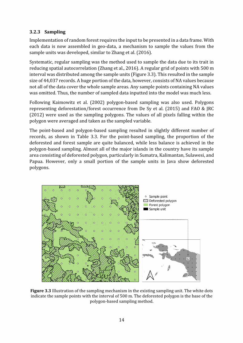
Systematic, regular sampling was the method used to sample the data due to its trait in

reducing spatial autocorrelation (Zhang et al., 2016). A regular grid of points with 500 m

interval was distributed among the sample units (Figure 3.3). This resulted in the sample

size of 44,037 records. A huge portion of the data, however, consists of NA values because

not all of the data cover the whole sample areas. Any sample points containing NA values was omitted. Thus, the number of sampled data inputted into the model was much less.

Following Kaimowitz et al. (2002) polygon-based sampling was also used. Polygons

representing deforestation/forest occurrence from De Sy et al. (2015) and FAO & JRC

(2012) were used as the sampling polygons. The values of all pixels falling within the

polygon were averaged and taken as the sampled variable.

The point-based and polygon-based sampling resulted in slightly different number of

records, as shown in Table 3.3. For the point-based sampling, the proportion of the

deforested and forest sample are quite balanced, while less balance is achieved in the

polygon-based sampling. Almost all of the major islands in the country have its sample

area consisting of deforested polygon, particularly in Sumatra, Kalimantan, Sulawesi, and

Papua. However, only a small portion of the sample units in Java show deforested polygons.

Figure 3.3 Illustration of the sampling mechanism in the existing sampling unit. The white dots indicate the sample points with the interval of 500 m. The deforested polygon is the base of the

polygon-based sampling method.

15

Table 3.3 Overview of the sampling result. Different sampling methods return different number of records. In agriculture direct driver, only smallholders and tree crops were dominant; there was not enough sample of commercial agriculture to be considered in the models.

Category # of features

Point Polygon

All 4621 4199

Deforested 2361 2482

Non-deforested 2260 1717

Agriculture 1311 1360

Smallholder 358 409

Tree crops 955 950

Other 1085 1079

Built-up 56 100

Water 11 26

3.2.4 Random forest model

Random forest model was developed by Breiman (2001). It is a machine learning

technique that constructs an ensemble of decision trees to conduct classification or

prediction (regression). Random forest employs the bagging method. This algorithm is

sensitive to the number of variables chosen to split the nodes (mtry) and the number of

decision trees constructed in the model (ntree).

In the first step, the algorithm constructs multiple decision trees ntree (Liaw and Wiener,

2002). At the nodes of each decision tree, the algorithm use a portion of the predictors

(mtry) by randomly sampling them. The result of every tree is then averaged, and the

prediction is inferred from them.

In this research, the models would be constructed with the main aim to predict whether

deforestation happened or not. Thus, the dependent variable is the deforestation

occurrence. It is categorical and binary; there is only two possible value on the dependent

variable, i.e., whether deforestation occurs or do not occur. The model will be constructed

such that the binary value is determined by the value of other independent variables,

which corresponds mostly to the indirect driver data. The number of the trees (ntree) is

500 by default, and the number of randomized variables is equal to the square root of the number of available variables.

The models were constructed multiple times to accommodate 1) different sampling

method (i.e., regular vs. polygon-based); 2) different variable combination and 3) detailed

assessment of different direct drivers. To reach the latter, a base model needed to be

constructed. Such models would built from the most effective indirect driver

combination. Some measures were conducted to come up with this base model, such as

variable reduction, detection of false predictor and accuracy analysis. Because not all of

the considered indirect drivers might be useful, measures to detect the significance of all

of the indirect drivers were also conducted so the ineffective indirect drivers can be

16

omitted. It is also important to detect potential false predictors. Finally, the models were

judged from its accuracy so that the most accurate model can be picked out.

Due to the randomization trait of random forest, each of the constructed model would

produce a slightly different classification result and accuracy. To achieve a more

consistent and reliable result, the averaged outcome of 50 runs of the model is used.

3.2.5 Result assessment

Assessment of the model can be made through the accuracy, and the out-of-bag (OOB)

estimate error rate. During the construction of the model, the initial dataset is partitioned

into 70:30 proportion of training and testing data. Accuracy shows the percentage of the validation dataset that was correctly predicted.

Each constructed tree in random forest also only utilizes around two-thirds of the

observations. The remaining data is not used to fit the tree; thus, it is called out-of-bag.

The result of the model is compared to the OOB, such that the test error can be estimated (Breiman and Cutler, 2003; James et al., 2013).

2.2.6 Variable Importance

This feature of random forest is useful to assess which variables (i.e., indirect drivers)

have the most significant role in classification. During the randomized selection of

variables in constructing the nodes, some variables are left out. The tree is constructed

without considering the left-out variables. After running the model, the trees are rerun

by also considering the left-out variable to produce another classification result. The

result are then compared with the original classification results, typically resulting in a

margin: the proportion of votes for its true class minus the maximum of the proportion

of votes for each of the other classes (Breiman and Cutler, 2003). The importance was

measured by averaging the lowering of the margin across all cases when a particular

variable is permuted. The larger the margin means, the more important a variable is. If

that particular variable is left out, the classification accuracy will greatly decrease.

Feature importance can also be measured through the Gini index, i.e. the measure of the

purity of a node. A smaller value indicates that a node is pure; the result of a single

dominant observation (James et al., 2013). Therefore, a split on the classification tree will

decrease the gini. Averaging all of the decreases in the forest caused by a particular

variable thus produce the Gini measure. Although it is known to be not as reliable as the

former measure, this feature may still be useful in assessing the importance of a variable

(Breiman and Cutler, 2003).

2.2.7 Partial Dependence

Partial dependence plot is method to show the effect of a feature into the outcome of a

machine learning model (Friedman, 2001). In this research, this plot can show the effect

of a particular indirect driver in predicting deforestation occurrence. Partial dependence

plot is visualized in a 2-axes graph. The x-axis depicts the independent variable of

interest. In the case of classification, the y-axis shows the marginal effect of a variable on

the class probability (Breiman et al., 2011). A positive value suggests that the particular

17

value of the independent variable is more likely to corresponds with the positive class of

the dependent variable, and vice versa.

3.3 Software

Most of the data processing and analysis were conducted within R (R Core Team, 2018).

R is a programming language which provides an environment for statistical computing

and graphics. Pre-processing, spatial data handling, and data visualization were

implemented in R using relevant packages. Implementation of random forest was done

through the ‘randomForest’ and ‘caret’ package (Kuhn, 2008; Liaw and Wiener, 2002). In

addition to model implementation, those packages were also utilised to review the model,

such as getting the model accuracy as well as assessing the variables in detail. These

assessments were visualised using package ‘ggplot’ (Wickham, 2016).

18

19

4. Results

4.1 Statistical properties of the indirect drivers

Table 4.1 presents the statistical overview of the indirect drivers. These statistics are only

computed for continuous indirect drivers (i.e., proximity, socioeconomic and

biophysical); categorical indirect drivers (i.e., zonation) is left out. In general, no

significant difference is observed between different sampling methods. Notable

differences are only observed in indirect drivers with high standard deviation, such as

distance to palm oil mills and GDP.

The average distance to both roads and rivers suggests that most of the deforestation

happened within 3-5 km proximity from these features. A similar pattern is also observed

in distance to concession zones: deforestation is more common in forests closer to

concession zones (Table 4.1). However, different observation is noticed in the distance to

palm oil mills and piers. For the point-based sample, the average distance to those

variables suggests that deforestation is more common in forests further away from palm

oil mills and piers, although the standard deviation themselves are relatively high.

As suggested by its high standard deviation, the socioeconomic variables tend to have

high variations. The histograms (Figure 4.1) show that the value tend to spread out, thus

confirming this finding. Notable gaps and patches are evident particularly in GDP and

HDI. The only socioeconomic variable with low standard deviation is the HDI. Different

sampling methods show the same average HDI of 70, either for forest or deforested area.

Different observations for different sampling methods were also observed. For GDP,

polygon-based sample shows deforested area is correlated with higher GDP (2642 bil.

compared to 2884 bil. on the forested area), while the point-based sample shows the

opposite (2515 bil. compared to 2450 bil. on the forested area).

Average precipitation suggests that deforestations are commonly occurring in areas

where the precipitation rate is higher (around 2700 mm/year compared to 2550-2600

mm/year for forested area). The standard deviation of this variable is also relatively low

(around 370-400 mm/year), suggesting that there is less variation. Looking at the

elevation, point-based sample suggests that deforestation tend to occur in higher

altitudes (121 m for forest, 160 m for deforested), while polygon-based sampling shows

the opposite (204 m for forest, 188 m for deforested). There is no significant difference

noted between forest/deforested region in temperature and slope. The average

temperature for both forest and deforested area is circa 26°C, and the slope is around 3-

5° steep.

20

Table 4.1 Statistical properties of the (a) point-based sampled and (b) polygon-based sampled

indirect drivers. These overviews seem to agree with the initial assumption, except for some

(greyed-out) variables. The deforested region was initially assumed to be associated with higher

socioeconomical properties and closer to the human-made structures.

(a)

Category Variable Mean Standard Deviation

Forest Deforested Forest Deforested

Distance

Concession logging (km) 81.2 66.8 77.7 55.7 Concession palm oil (km) 36.1 16.3 50.3 30.1 Concession wood fibre (km) 83.4 39.1 204.2 74.3 Palm oil mills (km) 89.4 97.5 165.6 211.7 Piers (km) 53.6 65.7 45.9 61.0 Ports (km) 79.4 62.5 47.9 43.8 River (km) 7.6 5.3 5.3 3.8 Roads (km) 7.7 3.1 8.3 4.9

Socioeconomic

GDP (IDR billion) 2884.5 2642.2 2398.5 2929.6 Population 423,737 319,552 276,052 220,539 HDI 70 70 3 4 People employed 168,308 135,398 98,571 85,964

Biophysical

Precipitation (mm/year) 2,569 2,703 373 390 Temperature (°C) 26.3 26.1 15 19 Elevation (m) 121 160 279 389 Slope (°) 3 3 5 6

(b)

Category Variable Mean Standard Deviation

Forest Deforested Forest Deforested

Distance

Concession logging (km) 74.0 63.4 78.3 56.6 Concession palm oil (km) 36.8 17.9 47.6 33.9 Concession wood fibre (km) 82.1 42.4 183.6 89.9 Palm oil mills (km) 123.1 104.5 243.5 230.1 Piers (km) 60.8 65.0 54.5 56.6 Ports (km) 79.7 64.1 49.1 47.2 River (km) 7.1 5.0 4.8 3.9 Roads (km) 8.5 3.3 8.5 5.3

Socioeconomic

GDP (IDR billion) 2450.6 2515.2 2099.3 2624.8 Population 367,692 324,067 266,800 218,305 HDI 70 70 3 5 People employed 148,700 138,314 96,265 86,465

Biophysical

Precipitation (mm/year) 2,631 2,725 451 402 Temperature (°C) 25.9 26 21 21 Elevation (m) 204 188 386 416 Slope (°) 5 4 7 6

21

Figure 4.1 Histogram of the point-sampled socioeconomic variables. Discrete distributions are observed, especially in GDP and population.

4.2 Model construction

The base model was determined by trying out different combination of indirect drivers

(Table 4.2). In total, three different combinations were tested to come up with the base

model. These combinations were determined according to the significance of each

indirect driver. Potential false predictor was also left out.

The model was initially constructed by incorporating all of the indirect drivers listed in

Table 3.2. Using these 20 indirect drivers, the significance of each considered indirect

driver is assessed from its average decrease of accuracy when the particular indirect

driver is removed from the model. As can be seen in Figure 4.2, both sampling methods

agree that the zonation indirect drivers are among the least significant predictors in the

model. This is followed by the socioeconomic indirect drivers, putting both categories

among the candidate of the removed indirect drivers.

A detailed assessment of precipitation suggests its role as a potential false predictor, as

identified from Figure 4.3. This partial dependence plot suggests that deforestation seem

to happen within a specific precipitation rate of 2700 mm. Downward spike around 2500

mm precipitation rate also suggest another specific value for forest area. While these

22

values coincide with the average precipitation rate indicated in Table 4.1, the overall

shape of the curve shows no variation; indicating strong evidence of false predictor.

The base model is thus constructed by removing these categories of indirect drivers:

zonation, socioeconomic and precipitation (Table 4.2). Each combination is tested on

both point-based and the polygon-based sample. Accuracy is used to judge the model

rather than the OOB error estimate, because between different models, there are only

minor differences on the OOB error estimate.

Overall, the models return good results with low error rate and high accuracy. As depicted

in Table 4.3, point-based models always return higher accuracy and lower OOB error

estimate. Around 2% difference of error estimate is observed between the two different

sampling methods, while the accuracy returns about 3% discrepancy. Excluding zonation

and precipitation saw an increase of accuracy by 0.08% in the point-based model but a

decrease of 0.33% for the polygon-based model. Further removal of the socioeconomic

variable was able to recover the accuracy by 0.14% in the polygon-based model. A slight

increase of 0.02% is also observed in the point-based model. All things considered, Model

3 is thus selected as the base model. Although accuracy-wise the polygon-based model

does not return the best accuracy, including false predictor is deemed to produce biased

result.

Using model 3 as the base model, four different direct driver-specific models were

constructed: 1) agriculture, 2) other drivers, 3) smallholder agriculture and 4) tree crop

agriculture. The last two models are constructed to assess the indirect drivers of

agricultural-driven deforestation in detail. The accuracy of these models is listed in Table

4.3. In all cases, the models are able to reach relatively high accuracy. It appears that the

effect of different sampling method is reduced here with both sampling method returning

similar accuracy; even the polygon-based model is more accurate than its counterpart. In

contrast to its base models, notable differences can be observed on the OOB error

estimate between the different direct driver models.

23

Figure 4.2 Variable importance plot for model 1 applied to (a) point-based sample and (b) polygon-based sample.

24

Figure 4.3 Partial dependence plot of precipitation.

Table 4.2 Variable combinations of each random forest model.

Variables Model 1 2 3 (Base) Agri Small Treecrop Other

Driver Agriculture

Smallholder

Tree crop Other

Zonation Concession logging

Concession palm oil Concession wood fibre Plantation

Distance Roads

River Ports Piers Palm oil mills Concession logging Concession palm oil Concession wood fibre

Socioeconomic Population

GDP HDI Employment

Biophysical Elevation

Slope Precipitation Temperature

25

Table 4.3 Overview of model accuracy. Because there are not many variations on the OOB error estimate between the model, the accuracy is used as the main judgement of the model.

Model OOB Accuracy (%)

Point Polygon Point Polygon 1 5.92% 7.66% 95.12% 92.56%

2 5.94% 7.64% 95.20% 92.23%

3 (Base) 5.96% 7.64% 95.22% 92.37%

Agriculture 3.72% 4.39% 96.21% 95.18%

Smallholder 5.37% 5.30% 93.57% 96.41%

Tree Crop 2.99% 4.11% 97.91% 97.33%

Others 6.23% 6.75% 94.59% 92.78%

4.3 Direct driver models

4.3.1 Variable importance

The overview of variable importance for the direct driver-specific models is visualised in

the heatmap in Figure 4.4. A detailed depiction of these are also visualised in variable

importance plot in Annex A. Between different direct drivers, variations of the order of

the most significant indirect drivers are spotted, indicating that specific circumstances

are only revealed when analysing the direct drivers in detail. In general, all of the models

agree that distance to palm oil mills is always among the most important, and slope is

always the least important. Other important variables include distance to roads and

elevation. It can be seen that in the base model, the mean decrease accuracy tends to be

in a higher value, while splitting the direct drivers into specific categories result in lower mean decrease accuracy.

In agriculture-driven deforestation, different magnitude of mean decrease accuracy is

identified between different sampling methods, but the composition of the top-5 indirect

driver stays the same. It includes elevation, distance to piers, palm oil mills, river, and

roads. Looking into specific agricultural direct drivers, smallholder agricultures seem to

be related to the presence of roads and river. On the other hand, tree crop agriculture is

most prominently related to the distance to palm oil mills, followed by distance to roads

and logging concession zones.

Both sampling methods agree that other direct drivers are associated with the distance

to palm oil mills. Compared to other models, biophysical parameters (i.e., elevation and

temperature) seem to take more importance in this model. Other significant indirect drivers include distance to logging concession zones and distance to ports.

26

Figure 4.4 Heat map of variable importance of (a) point-based model and (b) polygon-based model. The heatmap is coloured based on the mean decrease on accuracy when a particular variable is removed. A higher value corresponds to a more important variable.

4.3.2 Partial dependence

The partial dependence plots (PDP) of the most significant indirect drivers are presented

in Annex B. When interpreting the PDP, we are interested mainly with the trend of the

graph and the value of the x- and y-axis (Friedman, 2001; Sharma, 2017). In this research,

the y-axis shows how the likelihood of deforestation is changing with the change in the

given indirect driver (shown in the x-axis). Positive y-axis value means for that particular

value on the x-axis, the model is likely to predict deforestation. Negative value indicates

the opposite. If the y-axis value is zero, that particular indirect driver has no effect in the prediction outcome.

Clear trends are observed in the PDP of distance to road and distance to river. These PDPs

suggest that deforestation is more likely to occur nearby roads or rivers. The farther a

forest is from roads or river, the less likely deforestation to occur. Breaking up the data

into specific direct driver revealed that distance to roads and rivers have the strongest effect in predicting deforestation in the tree crop and other direct driver.

Different breakpoints (i.e. where the line crosses the x-axis) are observed between

different direct driver models, suggesting different effect of roads and rivers to specific

27

direct drivers. This might indicate the distance where the presence of a certain feature

loses its effect in constituting deforestation. For roads, it is observed that smallholder

agriculture and tree crop agriculture have lower breakpoint (< 5000 m) compared to

other direct driver. Higher breakpoints are observed in the distance to river, ranging from

5000-7500 m, with smallholder agriculture has the lowest breakpoint (around 5000 m).

For both roads and rivers, it is also noted that the peak probability is achieved circa 1000-

1500 m. This might suggest that deforestation does not necessarily occur right beside the

road/river, but at a certain distance from it.

Although analysis of the variable importance plots previously signified the importance of

distance to palm oil mills, the pattern indicated in its PDP is not as obvious as expected.

Relative to the base, agriculture and smallholder model, distance to palm oil mills is only

apparent in deforestation driven by tree crop agriculture (in 0-30 km) and other driver

(> 25 km).

The PDP of both distance to ports and distance to piers suggest that they have a mixing

effect on the deforestation occurrence. The effect of distance to port in predicting

deforestation is apparent within 0-25 km distance, while the effect of piers is notable

within 50-60 km distance. For both indirect drivers, the effect is strongest in the tree crop

and other driver model. Smallholder-driven deforestation is only slightly affected by the

distance to pier.

In the biophysical variables, specific pattern is again only revealed in the direct driver-

specific models. The base, agriculture and other direct driver model initially show no

significant pattern; the pattern is only revealed when looking into specific categories of

agriculture. Smallholder-driven deforestation is more likely to occur in higher elevation

(> 500 m) and in temperature range of 20-24°C. Tree crop-driven deforestation is more likely to happen in lower altitudes (100-250 m) and warmer temperature (25-26°C).

28

29

5. Discussions

5.1 Overview

This research assessed the link between the direct and indirect drivers of deforestation.

Models were initially constructed using two different sampling methods, i.e., point and

polygon-based sample. These two methods result in different accuracy and in general, the

point-based sample was able to deliver the higher accuracy. This might be addressed to

the trait of the sampling methods. In handling large areas, polygon-based sampling would

average the value of the whole area, thus generalizing the variables. In contrast, point-

based sampling is able to sample the extremes: higher/lower value would not be

dissolved. Despite this, similar trend and pattern are still observed in the variable

importance and partial dependence plot. Between the two different sampling methods,

the composition of the most important variable, as well as its marginal effect are still comparable.

All in all, initial assessment at the direct driver data suggests that most deforestation in

Indonesia is directly driven by agricultural and other direct drivers. Contrasting order of

importance of the indirect drivers are apparent when comparing the variable importance

plot of different models, suggesting that general deforestation model (i.e. base model) do

not always reflect the pattern shown in the driver-specific model. Apparently, these

hidden patterns are only revealed by constructing the model based on the specific direct driver. Some of the most important findings are described below.

5.2 Palm oil as a driver of deforestation

Though it does not always rank as the most important variable, the consistent

significance of distance to palm oil mill in each of the constructed model signifies the role

of palm oil in constituting deforestation. This finding seems to confirm the long-growing

perception of palm oil as a cause of deforestation in Indonesia. Koh and Wilcove (2008)

estimated that at least 56% of palm oil expansion in Indonesia is established in a formerly

natural forests-lands. A regional analysis in Southeast Asia found that at least 45% of the

palm oil plantations in the region were originally forests (Vijay et al., 2016). This role is

also underlined by Indrarto et al. (2012) in CIFOR’s Indonesia country report, where a

five-fold increase of palm oil estate area in the 90s was observed: from 1,652,301 ha in

1989 to 8,204,524 ha in 1998 (Sawit Watch, 2009).

The significance of distance to palm oil mills is particularly apparent in the tree crop and

other driver model. In both models, this variable ranks as the most important variable

with a clear gap of mean decrease accuracy value with the other variables. This provides

a compelling evidence that the tree crops in Indonesia is dominated by palm oil. While in

the data the scale of plantation is not distinguished, this palm oil-related deforestation is

most likely be dominated by large scale plantations. In their study, Lee et al. (2014), found

that in Indonesia, deforestation leading to palm oil establishment are mostly driven by

large-scale palm oil industry (89.2%), in contrast to smallholder (10.7%).

30

Distance to palm oil mills also acts as an important variable in the other driver models.

Looking at the data into detail, most of the other direct drivers here refer to other wooded

lands, mainly consisting of degraded forest and shrubs. The strong presence of distance

to palm oil mills in the other driver model suggests that these abandoned lands are eventually turned into palm oil plantations in the following years.

Several explanations can be attributed to this. First, it might be related to the

establishment of new moratoriums. While the demand for palm oil keeps on increasing,

the establishment of new moratoriums in 2010 prohibits local governments for granting

new concession licenses (Busch et al., 2015). This makes it harder for farmers to clear

new forests. However, this moratorium was often criticised, one of them for not covering

the secondary (degraded) forest (Murdiyarso et al., 2011). Exploiting existing degraded

forest or cleared land might be seen as the most reasonable option; thus providing a

strong explanation of this finding (Sheil et al., 2009).

Second, it is possible that this other land use is merely a step in the land use change

process. Boucher et al. (2011) outlined that forest logging is often followed by the

establishment of palm oil plantations. This is further confirmed by Romijn et al. (2013)

whose study found out that around 25% of open and degraded lands are eventually

converted into commercial agriculture. This is related to the third explanation, the result

of misused concession licenses for establishing plantations (Romijn et al., 2013). Many

companies used this license merely to clear the forest, sell the timbers, and then abandon

the lands. These wastelands, as referred by WWF Indonesia (2008), are then abandoned, covered by shrubs before eventually converted into palm oil plantations.

It is interesting to note the biophysical pattern found on the tree crop driver. The peaks

shown on the PDP of temperature and elevation correspond with some biophysical

suitability of palm oil. During their study in mapping palm oil suitability across Indonesia,

Pirker et al. (2016) used similar parameters, such as by setting the optimum

temperatures between 24-28 °C. Gingold et al. (2012) described altitudes below 500 m

as ‘highly suitable’ for palm oil plantations. While such biophysical variables are not the

most determinant variable in characterising palm oil plantations (thus relating it to

deforestation), it can be useful to a certain extent (Vijay et al., 2016).

Vijay et al. (2016) emphasised the need to “not relying solely on biophysical

requirements” to characterise palm oil expansion. They suggested to include proximity

to infrastructures to come up with better characterisation. These transportation

infrastructures (i.e., roads) rank amongst the important variables in the tree crop model,

thus confirming Vijay’s hypothesis.

5.3 Role of smallholder agriculture

The composition of the variable importance in smallholder model suggests that the

circumstances are more complex than in the tree crop agriculture, where palm oil is the

lone dominant direct driver. Here, distance to roads and rivers, as well as elevation play

a much greater role than palm oil mills. This is expected, as the categorization of

smallholder agriculture on the data does not include palm oil plantation. Hence, other

circumstances play a greater role here.

31

Lee et al. (2014) outlined that expansion of smallholder agricultures in Indonesia cover

various commodities such as rubber plantation, rice fields or rattan garden. The

biophysical variables attributed to smallholder agriculture tend to spread out and does

not specifically point out on a specific value, unlike the ones observed in the tree crops

model. The temperature ranges from 16-24 °C, and it tends to present in higher elevation

(500-2000 m). This suggests that the variety of commodities can be very diverse. Rice

might be preferred in the lowlands, while in the highlands cash crops (e.g., coffee and tea)

is also common (FAO, 2005). Perennial crops such as rubber tree are quite versatile, and

it has been associated with shifting agriculture practice, i.e., slash and burn system

especially in the highlands (FAO, 2005).

5.4 Direct and indirect drivers of deforestation in Indonesia

Constructing specific direct driver models produced different level of importance of

indirect drivers. For each direct driver, different indirect driver tends to also have

different marginal effect. These variations suggest that there are some links that are

specifically related between each direct and indirect driver.

The first link is notable from the transportation networks. In general, Miyamoto (2006)

outlined the strong role of road networks in determining deforestation is because roads

provide accessibility, thus reducing transportation cost and time of logistics. The role of

roads as a driver of deforestation is not new, and numerous studies have previously

emphasised the role (Barber et al., 2014; Miyamoto, 2006; Zhang et al., 2016). However,

it is interesting to note that in this research, the marginal effect of distance to roads is

only most apparent in the palm oil-related direct drivers (i.e., tree crops and other direct

drivers), and not in the smallholder direct driver. A possible explanation of this might be

related to the ability of large-scale palm oil industry to establish their own ‘unofficial’

road networks.

In their study, Barber et al. (2014) outlined that in addition to major roads, the presence

of ‘unofficial’ road networks can amplify the risk of deforestation. These roads were built

without official supervision and incentives from the government (Arima et al., 2005;

Brandão and Souza, 2006). In Indonesia, these roads are frequently established near

areas with vulnerable forests and agriculture activities (Sloan et al., 2018). In contrast to

smallholder agricultures that utilize existing ‘official’ road networks, large-scale

plantations might possibly establish their own road network, thus explaining the

significant marginal effect of distance to roads in tree crop and other direct driver.

Another link can be found in the role of distance to river. The role of river as a predictor

of deforestation has been underestimated in previous studies (Barber et al., 2014;

Laurance et al., 2002). However, this finding suggests that distance to rivers is

particularly important in predicting deforestations driven by smallholder agricultures.

This might be attributed to the farming system in Indonesia. Most of the farm system in

Indonesia is rain-fed agricultures, i.e., they rely on rain to irrigate the field. Additionally,

a relatively big portion (31.5%) of them uses irrigation system; utilizing natural

freshwater sources such as rivers and lakes to irrigate the crops (Devendra, 2016).

32

According to the CIA’s World Factbook, Indonesia has over 67 km2 of irrigated farmlands,

the 6th highest in the world (Central Intelligence Agency, 2009).

There is not enough evidence on the common use of navigable river as a mean of

transportation and logistics of agricultures, especially in Indonesia. In Indonesia, rivers

are only a common means of transporting extracted woods after deforestation (Bauch et

al., 2007; McCarthy, 2002).

5.5 Implications for REDD+

Detailed information regarding drivers of deforestation is vital for REDD+ activities to

succeed. While addressing these drivers are beyond the scope of this study, the methods

presented in this research have demonstrated an approach to analyse the link between

direct and indirect drivers of deforestation in Indonesia. Merely analysing deforestation

as a general model is deemed inadequate, because our results show that specific link to

indirect drivers are only revealed in the direct driver-specific models. This implies the need of detailed direct driver data as a prerequisite.

Prior studies have utilized land uses following deforestation as a proxy of direct driver

data (De Sy et al., 2015; Hosonuma et al., 2012). The present study has demonstrated the

usability of such proximate direct driver in linking them with indirect driver data. This

opens up a way to potentially analyse the link between direct and indirect drivers in

greater scale and greater detail. To achieve this, one may use detailed forest cover change

(Hansen et al., 2013a) or temporal land cover data (Bontemps et al., 2013; Jun et al.,

2014). The advances in earth observation system has also open up ways to detect forest

disturbance in near real-time, thus providing even more detailed data (Popkin, 2016;

Verbesselt et al., 2010). Detailed information on the link between direct and indirect

drivers can therefore help the countries in setting up their national strategies to

effectively address the drivers of deforestation.

5.6 Limitations and recommendations

5.6.1 Potential bias in variable importance and partial dependence plot

Random forest has been popularly used in geospatial domain. However, one should

consider some limitations in the method, especially during the interpretation of the

variable importance (Okun and Priisalu, 2007). Strobl et al. (2007) pointed out that the

algorithm’s variable importance measures can be unreliable when “potential predictor

variables vary in their scale of measurement or their number of categories”. Gislason et

al. (2006) also outlined the insensitivity of this method when dealing with noise and

overtraining. The false predictor role of precipitation in this research demonstrated this potential bias.

This research attempted to overcome this issue by making comparisons of the results to

preceding studies. While some of our results produce sensible outcomes, this might

explain the insignificant role of several variables throughout different models. Critical

assessment is thus a necessity in interpreting the results. Several studies have developed

improved random forest algorithm to tackle this issue, therefore future studies might be

33

directed into implementing such improved algorithms (Strobl et al., 2007; Zhang and Lu,

2012).

Molnar (2018) outlined several disadvantages of Partial Dependence Plot (PDP) to be

considered when interpreting such plots. First, PDPs do not show distribution. For

example, there might be some regions of the graph with actually no data that is

represented as straight line in the plot. This might lead to false conclusions. Second, PDPs

assume the independence of the assessed variable (i.e., indirect driver). This plot assumes

that one indirect driver is not correlated with another indirect driver. In reality, this is

mostly not the case. For example, population and economic growth often have positive correlation (Geist and Lambin, 2001).

5.6.2 Socioeconomic variables

Prior studies have indicated the importance of socioeconomic variables in modelling

deforestation, such as by incorporating GDP, population and employment rate (Kissinger

et al., 2012; Romijn et al., 2013; Vijay et al., 2016). An attempt to incorporate these

variables was made by using data from World Bank Group (2018). However, the

socioeconomic variables always rank low in the variable importance plot. There are

several possible explanations.

First, it is possible that the socioeconomic variables are simply not of importance in the

model. The effect of these variables in influencing deforestation might be too complex for

random forest to model, as the effect of socioeconomic variables in deforestation is not

very straightforward.

Second, this might be attributed to the quality of the data. Presenting the data in district

level means assuming that every area of a district is homogeneous, having the same value.

In reality, this is not always the case; the different neighbourhood of a city, for instance,

would always have different population densities. The same case applies to other

socioeconomic variables such as HDI or GDP. In spatial analysis, one way to present

continuous data is through raster. With each pixel representing a snippet of an area, a

specific value can be attributed to them. Currently, such gridded socioeconomic data is

rare; even if there is any, they are often presented in poor resolution, and the range of the

available socioeconomic variable is limited such as the population estimate grid

produced by NASA SEDAC (Socioeconomic Data and Application Center).

5.6.3 Categorical variables and other potential drivers

Seen from the variable importance across the models, in general, categorical (i.e., binary)

variables are not good predictors of deforestation. Initially, these variables were expected

to be able to represent the concession zones, as one of the policy factors governing

deforestation. The considered concession zones in this research are the main industrial

causes of deforestation in Indonesia, i.e. palm oil, wood fibre and logging (Abood et al.,

2015). In fact, between these three industries, palm oil is actually the direct driver with

the least impact in terms of forest loss between 2000-2010. Fibre plantation and logging

have greater disturbance, responsible for 1.9 Mha and 1.8 Mha of forest loss, respectively.

Excluding these variables means that they are not represented well in the model. As a

result, detailed assessment of the drivers was only able to be conducted on palm oil,

34

because the distance to palm oil mills seems to be very decisive in constructing the model.

In future studies, it is suggested to include also variables related to the other drivers.

Continuous, rather than categorical variable would be recommended. Potential features

may include, for example, distance to pulp factories or logging mills.

35

6. Conclusions

The present study was conducted to assess the link between direct and indirect drivers

of deforestation in Indonesia. Random forest-based spatial analysis of deforestation

drivers revealed that factors affecting different direct drivers could vary. In general, tree

crop driven deforestation is dominated by palm oil; particularly in large scale tree

plantations and is linked with the presence of palm oil mills and roads. In contrast to the

tree crop direct driver, the smallholder direct driver does not point out to a specific crop

type; it is rather a complex driver and may be associated with different categories of

agriculture, such as cash crops, perennial plants or swidden agriculture. In addition to

roads, smallholder agriculture is linked with the distance to river as its underlying driver

of deforestation.

Although some results have indicated specific biophysical characteristics for specific

direct drivers of deforestation, biophysical variables are less determinant compared to

the distance variables. The significance of socioeconomic variables as underlying driver

of deforestation was also not observed in this study.

The method proposed in this study can possibly be extended to greater level of detail,

such as to be implemented in nation-wide monitoring. This implies the need of detailed

direct driver data, so that the deforestation can be distinguished. Future studies might be

directed into producing and including continuous socioeconomic variables. Including

more factors concerning other potential indirect drivers (i.e., logging and wood fibre)

would also be useful. Due to the lack of data, this study has not been able to analyse in

detail regarding smallholder agricultures. Given its dominant role, one can conduct

detailed spatial analysis specifically in this type of agriculture to reveal the hidden

circumstances, e.g., the specific types of crops that cause deforestation.

Nevertheless, this study demonstrated the utilization of spatial analysis in analysing

deforestation. Proximity and spatial distribution are among the spatial properties of

forest clearing, and spatial analysis can be a useful instrument in studying deforestation.

The findings made in this study can contribute to countries in setting up effective and

efficient REDD+ strategies.

36

37

References

Abood, S.A., Lee, J.S.H., Burivalova, Z., Garcia‐Ulloa, J., Koh, L.P., 2015. Relative contributions of the logging, fiber, oil palm, and mining industries to forest loss in Indonesia. Conservation Letters 8, 58-67.

Achard, F., Beuchle, R., Mayaux, P., Stibig, H.J., Bodart, C., Brink, A., Carboni, S., Desclée, B., Donnay, F., Eva, H.D., Lupi, A., Raši, R., Seliger, R., Simonetti, D., 2014a. Determination of tropical deforestation rates and related carbon losses from 1990 to 2010. Global Change Biology 20, 2540-2554.

Achard, F., Boschetti, L., Brown, S., Brady, M., DeFries, R., Grassi, G., Herold, M., Mollicone, D., Mora, B., Pandey, D., 2014b. A sourcebook of methods and procedures for monitoring and reporting anthropogenic greenhouse gas emissions and removals associated with deforestation, gains and losses of carbon stocks in forests remaining forests, and forestation. GOFC-GOLD.

AFP, 2008. Indonesia looks to Papua to expand palm oil plantations: officials. AFP.

Angelsen, A., 2008. How do we set the reference levels for REDD payments?, Moving ahead with REDD: issues, options and implications, pp. 53-64.

Angelsen, A., Brown, S., Loisel, C., 2009. Reducing emissions from deforestation and forest degradation (REDD): an options assessment report.

Apan, A., Suarez, L.A., Maraseni, T., Castillo, J.A., 2017. The rate, extent and spatial predictors of forest loss (2000–2012) in the terrestrial protected areas of the Philippines. Applied geography 81, 32-42.

Applegate, G., Chokkalingam, U., Suyanto, S., 2001. The underlying causes and impacts of fires in south-east Asia. Center for International Forestry Research, International Center for Agroforestry Research, United States Agency for International Development, US Forest Service: Bogor, Indonesia.

Arima, E.Y., Walker, R.T., Perz, S.G., Caldas, M., 2005. Loggers and forest fragmentation: Behavioral models of road building in the Amazon basin. Annals of the Association of American Geographers 95, 525-541.

Barber, C.P., Cochrane, M.A., Souza Jr, C.M., Laurance, W.F., 2014. Roads, deforestation, and the mitigating effect of protected areas in the Amazon. Biological conservation 177, 203-209.

Bauch, S.C., Amacher, G.S., Merry, F.D., 2007. Costs of harvesting, transportation and milling in the Brazilian Amazon: Estimation and policy implications. Forest Policy and Economics 9, 903-915.

Bontemps, S., Defourny, P., Radoux, J., Van Bogaert, E., Lamarche, C., Achard, F., Mayaux, P., Boettcher, M., Brockmann, C., Kirches, G., 2013. Consistent global land cover maps for climate modelling communities: current achievements of the ESA’s land cover CCI, Proceedings of the ESA Living Planet Symposium, Edimburgh, pp. 9-13.

Boucher, D., Elias, P., Lininger, K., May-Tobin, C., Roquemore, S., Saxon, E., 2011. The root of the problem: what's driving tropical deforestation today? The root of the problem: what's driving tropical deforestation today?

Brandão, A., Souza, C., 2006. Mapping unofficial roads with Landsat images: a new tool to improve the monitoring of the Brazilian Amazon rainforest. International Journal of Remote Sensing 27, 177-189.

38

Bray, D.B., Duran, E., Ramos, V.H., Mas, J.-F., Velazquez, A., McNab, R.B., Barry, D., Radachowsky, J., 2008. Tropical deforestation, community forests, and protected areas in the Maya Forest. Ecology and Society 13.

Breiman, L., 2001. Random forests. Machine learning 45, 5-32.

Breiman, L., Cutler, A., 2003. Setting up, using, and understanding random forests V4. 0. University of California, Department of Statistics.

Breiman, L., Cutler, A., Liaw, A., Wiener, M., 2011. Package randomForest. Software available at: http://stat-www.berkeley.edu/users/breiman/RandomForests.

Burrough, P.A., McDonnel, R.A., 1998. Principles of Geographical Information Systems.

Busch, J., Ferretti-Gallon, K., Engelmann, J., Wright, M., Austin, K.G., Stolle, F., Turubanova, S., Potapov, P.V., Margono, B., Hansen, M.C., 2015. Reductions in emissions from deforestation from Indonesia’s moratorium on new oil palm, timber, and logging concessions. Proceedings of the National Academy of Sciences 112, 1328-1333.

Canadell, J.G., Raupach, M.R., 2008. Managing forests for climate change mitigation. science 320, 1456-1457.

Central Intelligence Agency, 2009. The CIA world factbook 2010. Skyhorse Publishing Inc.

Corley, R., 2009. How much palm oil do we need? Environmental Science & Policy 12, 134-139.

De Sy, V., 2016. Remote sensing of land use and carbon losses following tropical deforestation.

De Sy, V., Herold, M., Achard, F., Beuchle, R., Clevers, J.G.P.W., Lindquist, E., Verchot, L., 2015. Land use patterns and related carbon losses following deforestation in South America. Environmental Research Letters 10.

Devendra, C., 2016. Rainfed agriculture: its importance and potential in global food security.

FAO, 2005. Fertilizer use by crop in Indonesia, Rome, Italy.

FAO, 2012. State of the World's Forests Report, Rome.

FAO, 2015. Global Forest Resources Assessment.

FAO & JRC, 2012. Global forest land-use change 1990-2005. FAO, Rome (Italy).

Fick, S.E., Hijmans, R.J., 2017. WorldClim 2: new 1‐km spatial resolution climate surfaces for global land areas. International journal of climatology 37, 4302-4315.

FoodReg and WRI, 2018. Palm oil mills.

Friedman, J.H., 2001. Greedy function approximation: a gradient boosting machine. Annals of statistics, 1189-1232.

Gaveau, D.L., 2017. What a difference 4 decades make: Deforestation in Borneo since 1973. CIFOR.

Geist, H.J., Lambin, E.F., 2001. What drives tropical deforestation. LUCC Report series 4, 116.

Geist, H.J., Lambin, E.F., 2002. Proximate Causes and Underlying Driving Forces of Tropical Deforestation. BioScience 52, 143-150.

Gingold, B., Rosenbarger, A., Muliastra, Y., Stolle, F., Sudana, I.M., Manessa, M., Murdimanto, A., Tiangga, S., Madusari, C., Douard, P., 2012. How to identify degraded land for sustainable palm oil in Indonesia. Washington, DC: World Resources Institute.

39

Gislason, P.O., Benediktsson, J.A., Sveinsson, J.R., 2006. Random forests for land cover classification. Pattern Recognition Letters 27, 294-300.

Global Forest Watch, 2018a. Managed forest concessions.

Global Forest Watch, 2018b. Palm oil concession.

Global Forest Watch, 2018c. Tree plantations, in: Watch, G.F. (Ed.).

Global Forest Watch, 2018d. Wood fibre concessions.

Grassi, G., Monni, S., Federici, S., Achard, F., Mollicone, D., 2008. Applying the conservativeness principle to REDD to deal with the uncertainties of the estimates. Environmental Research Letters 3, 035005.

Hansen, M.C., Potapov, P.V., Moore, R., Hancher, M., Turubanova, S., Tyukavina, A., Thau, D., Stehman, S., Goetz, S., Loveland, T.R., 2013a. High-resolution global maps of 21st-century forest cover change. science 342, 850-853.

Hansen, M.C., Potapov, P.V., Moore, R., Hancher, M., Turubanova, S.A., Tyukavina, A., Thau, D., Stehman, S.V., Goetz, S.J., Loveland, T.R., Kommareddy, A., Egorov, A., Chini, L., Justice, C.O., Townshend, J.R.G., 2013b. High-resolution global maps of 21st-century forest cover change. Science 342, 850-853.

Hansen, M.C., Stehman, S.V., Potapov, P.V., Arunarwati, B., Stolle, F., Pittman, K., 2009. Quantifying changes in the rates of forest clearing in Indonesia from 1990 to 2005 using remotely sensed data sets. Environmental Research Letters 4.

Hosonuma, N., Herold, M., De Sy, V., De Fries, R.S., Brockhaus, M., Verchot, L., Angelsen, A., Romijn, E., 2012. An assessment of deforestation and forest degradation drivers in developing countries. Environmental Research Letters 7.

Indonesian REDD+ Task Force, 2012. REDD+ National Strategy, Jakarta.

Indrarto, G.B., Murharjanti, P., Khatarina, J., Pulungan, I., Ivalerina, F., Rahman, J., Prana, M.N., Resosudarmo, I.A.P., Muharrom, E., 2012. The context of REDD+ in Indonesia: drivers, agents and institutions. Cifor.

James, G., Witten, D., Hastie, T., Tibshirani, R., 2013. An introduction to statistical learning. Springer.

Jarvis, A., Reuter, H.I., Nelson, A., Guevara, E., 2008. Hole-filled SRTM for the globe Version 4.

Jun, C., Ban, Y., Li, S., 2014. China: Open access to Earth land-cover map. Nature 514, 434.

Kaimowitz, D., Angelsen, A., 1998. Economic models of tropical deforestation: a review. Cifor.

Kaimowitz, D., Mendez, P., Puntodewo, A., Vanclay, J.K., 2002. Spatial regression analysis of deforestation in Santa Cruz, Bolivia.

Kissinger, G., Herold, M., De Sy, V., 2012. Drivers of deforestation and forest degradation: a synthesis report for REDD+ policymakers. Lexeme Consulting.

Klute, M., 2008. Forests in Papua: Data and Facts, Forest Conference of West Papua in Witten, Germany.

Koh, L.P., Wilcove, D.S., 2008. Is oil palm agriculture really destroying tropical biodiversity? Conservation letters 1, 60-64.

Kuhn, M., 2008. Building predictive models in R using the caret package. Journal of statistical software 28, 1-26.

Laurance, W.F., 2007. Forest destruction in tropical Asia. Current Science, 1544-1550.

40

Laurance, W.F., Albernaz, A.K., Schroth, G., Fearnside, P.M., Bergen, S., Venticinque, E.M., Da Costa, C., 2002. Predictors of deforestation in the Brazilian Amazon. Journal of biogeography 29, 737-748.

Lee, J.S.H., Abood, S., Ghazoul, J., Barus, B., Obidzinski, K., Koh, L.P., 2014. Environmental impacts of large‐scale oil palm enterprises exceed that of smallholdings in Indonesia. Conservation letters 7, 25-33.

Liaw, A., Wiener, M., 2002. Classification and regression by randomForest. R news 2, 18-22.

Malhi, Y., Wright, J., 2004. Spatial patterns and recent trends in the climate of tropical rainforest regions. Philosophical Transactions of the Royal Society of London B: Biological Sciences 359, 311-329.

Margono, B.A., Potapov, P.V., Turubanova, S., Stolle, F., Hansen, M.C., 2014. Primary forest cover loss in Indonesia over 2000–2012. Nature Climate Change 4, 730.

McCarthy, J.F., 2002. Turning in circles: district governance, illegal logging, and environmental decline in Sumatra, Indonesia. Society &Natural Resources 15, 867-886.

Meijer, J., Huijbregts, M.A., Schotten, K., Schipper, A., 2018. Global patterns of current and future road infrastructure. Environmental Research Letters.

Minang, P.A., Van Noordwijk, M., Duguma, L.A., Alemagi, D., Do, T.H., Bernard, F., Agung, P., Robiglio, V., Catacutan, D., Suyanto, S., Armas, A., Silva Aguad, C., Feudjio, M., Galudra, G., Maryani, R., White, D., Widayati, A., Kahurani, E., Namirembe, S., Leimona, B., 2014. REDD+ Readiness progress across countries: time for reconsideration. Climate Policy 14, 685-708.

Miyamoto, M., 2006. Forest conversion to rubber around Sumatran villages in Indonesia: Comparing the impacts of road construction, transmigration projects and population. Forest Policy and Economics 9, 1-12.

Molnar, C., 2018. Interpretable machine learning: A guide for making black box models explainable. Christoph Molnar, Leanpub.

Murdiyarso, D., Dewi, S., Lawrence, D., Seymour, F., 2011. Indonesia’s forest moratorium: A stepping stone to better forest governance? Cifor.

Nakakaawa, C.A., Vedeld, P.O., Aune, J.B., 2011. Spatial and temporal land use and carbon stock changes in Uganda: implications for a future REDD strategy. Mitigation and Adaptation Strategies for Global Change 16, 25-62.

Okun, O., Priisalu, H., 2007. Random forest for gene expression based cancer classification: overlooked issues, Iberian Conference on Pattern Recognition and Image Analysis. Springer, pp. 483-490.

Palmer, C., 2001. The extent and causes of illegal logging: An analysis of a major cause of tropical deforestation in Indonesia.

Pan, Y., Birdsey, R.A., Phillips, O.L., Jackson, R.B., 2013. The structure, distribution, and biomass of the world's forests. Annual Review of Ecology, Evolution, and Systematics 44, 593-622.

Pirker, J., Mosnier, A., Kraxner, F., Havlík, P., Obersteiner, M., 2016. What are the limits to oil palm expansion? Global Environmental Change 40, 73-81.

Popkin, G., 2016. Satellite alerts track deforestation in real time. Nature News 530, 392.

R Core Team, 2018. R: A language and environment for statistical computing. R Foundation for Statistical Computing.

41

Rademaekers, K., Eichler, L., Berg, J., Obersteiner, M., Havlik, P., 2010. Study on the evolution of some deforestation drivers and their potential impacts on the costs of an avoiding deforestation scheme. Prepared for the European Commission by ECORYS and IIASA. Rotterdam, Netherlands.

Rautner, M., Leggett, M., Davis, F., 2013. The little book of big deforestation drivers. Global Canopy Programme: Oxford.

Romijn, E., Ainembabazi, J.H., Wijaya, A., Herold, M., Angelsen, A., Verchot, L., Murdiyarso, D., 2013. Exploring different forest definitions and their impact on developing REDD+ reference emission levels: A case study for Indonesia. Environmental Science & Policy 33, 246-259.

Rudel, T.K., Defries, R., Asner, G.P., Laurance, W.F., 2009. Changing drivers of deforestation and new opportunities for conservation. Conservation Biology 23, 1396-1405.

Salvini, G., Herold, M., De Sy, V., Kissinger, G., Brockhaus, M., Skutsch, M., 2014. How countries link REDD+ interventions to drivers in their readiness plans: Implications for monitoring systems. Environmental Research Letters 9.

Sawit Watch, 2009. Peta Investigasi Sawit Watch, Bogor.

Sharma, V., 2017. Quick Introduction to Partial Dependence Plots.

Sheil, D., Casson, A., Meijaard, E., Van Noordwijk, M., Gaskell, J., Sunderland-Groves, J., Wertz, K., Kanninen, M., 2009. The impacts and opportunities of oil palm in Southeast Asia: What do we know and what do we need to know? Center for International Forestry Research Bogor, Indonesia.

Sloan, S., Campbell, M.J., Alamgir, M., Collier-Baker, E., Nowak, M.G., Usher, G., Laurance, W.F., 2018. Infrastructure development and contested forest governance threaten the Leuser Ecosystem, Indonesia. Land Use Policy 77, 298-309.

Strobl, C., Boulesteix, A.-L., Zeileis, A., Hothorn, T., 2007. Bias in random forest variable importance measures: Illustrations, sources and a solution. BMC bioinformatics 8, 25.

Sunderlin, W.D., Resosudarmo, I.A.P., 1997. Laju dan penyebab deforestasi di Indonesia: penelaahan kerancuan dan penyelesaiannya. CIFOR, Bogor, Indonesia.

Sunderlin, W.D., Resosudarmo, I.A.P., Rianto, E., Angelsen, A., 2000. The effect of Indonesia's economic crisis on small farmers and natural forest cover in the outer islands. CIFOR Bogor, Indonesia.

UNFCCC, 2007. Bali Action Plan, Decision 1/CP. 13, COP13, Bali, Indonesia.

UNFCCC, 2009. Methodological guidance for activities relating to reducing emissions from deforestation and forest degradation and the role of conservation, sustainable management of forests and enhancement of forest carbon stocks in developing countries. Decision.

UNFCCC, 2014. Report of the Conference of the Parties on its nineteenth session, held in Warsaw from 11 to 23 November 2013. United Nations Framework Convention on Climate Change Bonn.

UNFCCC, 2018. REDD+ Fact Sheet.

Verbesselt, J., Hyndman, R., Newnham, G., Culvenor, D., 2010. Detecting trend and seasonal changes in satellite image time series. Remote Sensing of Environment 114, 106-115.

42

Vijay, V., Pimm, S.L., Jenkins, C.N., Smith, S.J., 2016. The impacts of oil palm on recent deforestation and biodiversity loss. PloS one 11, e0159668.

Wickham, H., 2016. ggplot2: elegant graphics for data analysis. Springer.

World Bank Group, 2018. INDO-DAPOER.

WWF Indonesia, 2008. Deforestation, forest degradation, biodiversity loss and CO2 emissions in Riau, Sumatra, Indonesia. One Indonesian Province’s Forest and Peat Soil Carbon loss over a Quarter Cebtury and its Plans for the Future.

Zhang, G., Lu, Y., 2012. Bias-corrected random forests in regression. Journal of Applied Statistics 39, 151-160.

Zhang, Y., Li, J., Qin, Q., 2016. Identification of Factors Influencing Locations of Tree Cover Loss and Gain and Their Spatio-Temporally-Variant Importance in the Li River Basin, China. Remote Sensing 8, 201.

43

Annex A: Variable importance plot

The variable importance plots of each of the constructed model is presented here. It can

be noted that different direct drivers have different order of importance of indirect

drivers. For example, in the general (base) model, distance to roads does not seem to have

high importance value. The importance is only revealed in the direct driver specific

model, that roads are of high importance in the agriculture (i.e. smallholder and tree crops) but not in the other direct driver.

Base model

Agriculture

44

Smallholder agriculture

Tree crop

Other drivers

45

Annex B: Partial dependence plot

Elevation

The influence of elevation as indirect driver in constituting deforestation is almost zero in the base, agriculture and other direct driver model. The

effect is only apparent in specific direct drivers: smallholder agriculture and tree crops agriculture. Smallholder-driven deforestation tend to occur in

higher altitudes (500-2000 m) and tree crops-driven deforestation is only apparent in lower altitudes (~150 m).

47

Temperature

Temperature seem to constitute deforestation in all direct drivers. Only the range between different direct drivers is different: in almost all direct

drivers, 26.5°C is the most common temperature where deforestation occur. Only in smallholder agriculture-driven deforestation the range of

temperature tend to spread out, between 16-26°C.

48

Distance to Roads

The effect of distance to roads as indirect driver of deforestation shows almost a negative linear relationship in all direct drivers. The probability of

deforestation decreases the further a forest is from roads. This effect is most apparent in the tree crop driven deforestation. The breakpoints suggest

that this underlying driver has effect around 0-5 km.

49

Distance to Piers

Distance to piers have mixing effects in different direct drivers. This indirect driver is most apparent in tree crop and other direct driver-related deforestation. The model is more likely to predict deforestation in the farther distances (> 50 km), except for the other direct driver, where the peak is observed in the distance around 25 km.

50

Distance to Ports

Distance to ports have similar effect to distance to piers. While it seems to have no effect in constituting smallholder driven-deforestation, its influence is very apparent in the tree crop and other direct drivers (between 0-50 km).

51

Distance to River

Similar to distance to roads, distance to river also have negative linear relationship with the probability of deforestation. The effect is more or less of the same magnitude for every direct driver. The effect of this indirect driver is apparent within 5-7.5 km radius from river.

52

Distance to Palm Oil Mills

While the variable importance plot for different direct driver signified the high importance of distance to palm oil mills, the PDPs of this indirect driver are not showing striking pattern. However, these plots agree that the effect of distance to palm oil mills is only apparent in the tree crop agriculture and other direct drivers.

53

Distance to Logging Concession Zones

As suggested by the peak, these plots suggest that deforestation is more likely to happen in forests nearby the logging concession zone (between 0-75 km). There is less probability of deforestation in farther distance. Every direct driver shows similar pattern, suggesting that the effect is almost identical for different direct drivers.

54

Distance to Wood Fibre Concession Zones

Distance wood fibre concession zones have minor influence in constituting deforestation agriculture and smallholder-driven

deforestation, and seem to have the strongest effect in the other driver model. In contrast, it has no effect in constituting deforestation in tree crop-driven deforestation.