APLICATION OF FRACTIONAL ALGORITMS IN THE CONTROL OF AN HELICOPTER SYSTEM

J. Coelho1, R. Matos Neto1, C. Lebres1, H. Fachada1, N. M. Fonseca Ferreira1

E. J. Solteiro Pires2, J. A. Tenreiro Machado3

1Polytechnic Institute of Coimbra, Institute of Engineering of Coimbra,

Dept. of Electrical Engineering, Quinta da Nora, Apartado 10057 3031-601 Coimbra Codex, Portugal,

2University of Trás-os Montes e Alto-Douro, Dept. of Engineering Quinta de Prados, Apartado 202, 5000 Vila Real, Portugal

3 Polytechnic Institute of Porto, Institute of Engineering of Porto, Rua Dr Ant. Bernardino de Almeida, 4200���072 Porto, Portugal

e-mail: joaobcoelho@hotmail.com, e-mail: rofdolfonneto@gmail.com, e-mail:clebres@isec.pt 1e-mail: nunomig@isec.pt, 2e-mail: epires@utad.pt, 3email: jtm@isep.ipp.pt

Abstract: This paper compares the application of fractional and integer order controllers for a laboratory helicopter twin rotor MIMO system using the MatLab package.

Keywords: Helicopter, Mathematic Model, Position Control, Fractional Control.

1. INTRODUCTION In this study we consider the dynamics of the helicopter system with two degrees of freedom (2-DOF) [1, 2]. The simulation and the real-time experiments in closed loop are performed and several comparisons are presented. Figure 1 shows a laboratory model of the Twin Rotor.

Figure 1 - Two views of the twin rotor MIMO System. At both ends of a beam, there are two propellers driven by DC motors, the beam is joined to its base though with an articulation. The articulated joint allows the beam to rotate so that its ends move on spherical surfaces. A counter-weight fixed to the beam determines a stable equilibrium position. The rotors are positioned perpendicularly to each other, so that the movements in the vertical and horizontal planes are only affected by the thrust one propeller. The controls of the system consist in the supply voltages of the motors. The measured signals are the two position angles that determine the position of the beam in space and the angular velocities of the rotors. The positions are measured using incremental encoders, and the angular

velocities are reconstructed by a simple differentiation and a second-order filtering of the measured position angles. This paper presents several control techniques for a lab helicopter model. It is adopted the Twin Rotor Mimo System (Feedback – TRMS) and are compared integer and fractional order control algorithms. The paper is organize as follow. Section two, provides an overview of the system model. Section three shows the conventional integer and the fractional order algorithms. Section four presents the simulations results. Finally, section five outlines some conclusions. 2. MATHEMATICAL MODEL First, we consider the rotation of the beam in a vertical plane that is around the horizontal axis. The helicopter has 2-DOF, the rotation of the helicopter body with respect to the horizontal axis and the rotation around the vertical axis, which are measured by two sensors. Each axis has one potentiometer for measuring the angle. The helicopter can move the horizontal axis, in the range �170º <�h< 170º, and the vertical axis, within �60º <�h< 60º, in pitch. The inputs are the voltages Uh and Uv affecting the main and tail rotor. The output command must match the capabilities of the hardware board that is capable to outputing [0, 5] Volt signal. This signal is shifted in the amplifier to create �2.5 Volt capability required to command the drive motor in both directions. When no control signals are applied, the helicopter will tend to position at �h = � 60º.

Table I – List of symbols

Protection

Beam of two degres of freedom Counter Balance

Protection

Tail Rotor

Variable Description Units [SI]

�hHorizontal position (azimuth position) of the model beam

[rad]

�hAngular velocity (azimuth velocity) of the model beam

[rad/s]

UhHorizontal DC-motor voltage control input

[V]

GhLinear transfer function of tail rotor DC-motor

H Non-linear part of DC- motor with tail rotor

[rad/s]

�h Rotational speed of tail rotor [rad/s]

Main Rotor Optical Encoders

FhNon-linear function (quadratic) of aerodynamic force from tail rotor

[N]

lhEffective arm of aerodynamic force from tail rotor

[m]

JhNon-linear function of moment of inertia with respect to vertical axis

[Kg.m2]

Mh Horizontal turning torque [N.m] Kh Horizontal angular momentum [N.m.s]

fhMoment of friction force in vertical axis

[N.m]

�vVertical position (Pitch position) of the model beam

[rad]

�vAngular velocity (Pitch velocity) of the model beam.

[rad/s]

UvVertical DC-motor voltage control input

[V]

GvLinear transfer function of main rotor DC-motor

v Non-linear part of DC-motor with main rotor

[rad/s]

�vRotational speed of main rotor [rad/s]

FvNon-linear function (quadratic) of aerodynamic force from main rotor

[N]

lvArm of aerodynamic force from main rotor

[m]

JvMoment of inertia with respect to horizontal axis

[Kg.m2]

Mv Vertical turning moment [N.m] Kv Vertical angular momentum [N.m.s]

fvMoment of friction force in horizontal axis

[N.m]

f Vertical turning moment from counterbalance

[N.m]

JhvVertical angular momentum from tail rotor

[N.m.s]

JvhHorizontal angular momentum from tail rotor

[N.m.s]

gvhNon-linear function (quadratic) of reaction turning

[N.m]

ghvNon-linear function (quadratic) of reaction turning

[N.m]

t Time [s] L Laplace Operator z Transform variable

The physical model is developed under some simplifying assumptions. It is assumed that friction is of the viscous type and that the propeller air subsystem can be described in accordance with the postulates of flow theory. First, we consider the rotation of the beam in the vertical plane, around the horizontal axis. Having in mind that the driving torques are produced by the propellers, the rotation can be described in principle as the motion of a pendulum. From the Newton second law of motion we obtain:

2

2

dtdJM v

vv�

�

(1)

�

�4

1iviv MM (2)

�

�8

1iviv JJ (3)

Figure 2 – The twin rotor mimo system. To determine the moments of gravity applied to the beam, making it rotate around the horizontal axis, we consider the situation of in figure 3, and:

� vvv CBAgM �� sincos1 ��� (4a)

ttstrt lmmmA �

�

��� ���

2 (4b)

mmsmrm lmmmB �

�

��� ���

2 (4c)

cbcbbb lmlmC ��

2 (4d)

Table II – The parameters of the Helicopter.

Variable Value Units [SI] mmr 0.228 [kg] mm 0.0145 [kg] mtr 0.206 [kg] mt 0.10166 [kg] mcb 0.068 [kg] mb 0.022 [kg] mms 0.225 [kg] mts 0165 [kg] lm 0.24 [m] lt 0.25 [m] lb 0.26 [m] lcb 0.13 [m] rms 0.155 [m] rts 0.10 [m]

where rms is the radius of the main shield and rts is the radius of the tail shield. Also:

� �mvmv FlM ��2 (5) where Fv(�m) denotes the dependence of the propulsive force on the angular velocity of the rotor.

� � vvhv CBAM �� cossin2

3 ����� (6)

dtd h

h�

��

(7)

To determine the moments of propulsive forces applied to the beam consider the situation given in figure 3.

Vertical Axis of rotation

�h

Mhl

Fh(�m)Tail Rotor

lm

lt

x

y

Figure 3 – Gravity forces in the TRMS, corresponding to the return torque, which determines the equilibrium position of the system. Finaly:

vvv KM ���4 (8) Figure 4 – Propulsive force moment and friction moment in the TRMS.

dtd vh

v�

�� (9)

where �v is the angular velocity around the horizontal axis and Kv is a constant. According to figure 4 we can determine components of the moment of inertia relative to the horizontal axis. Notice, that this moment is independent of the position of the beam.

21 mmrv lmJ � (10a)

3

2

2m

mvlmJ �

(10b)

23 cbcbv lmJ � (10c)

3

2

4b

bvlmJ �

(10d)

25 ttrv lmJ � (10e)

3

2

6t

tvlmJ �

(10f)

227 2 mmsms

msv lmrmJ ��

(10g)

228 ttststsv lmrmJ �� (10h)

mcbg lb

lcb

mtg

mtsg +

mtrg

lt

lm Main Rotor

Horizontal Axis

mmsg +

mmrg

Tail Rotor

mmg

mbg

�v

y

x Similarly, we can describe the motion of the beam around the vertical axis, having in mind that the driving torques are produced by the rotors and that the moment of inertia depends on the pitch angle of the beam. The horizontal motion of the beam (around the vertical axis) can be described as a rotational motion of a solid mass:

2

2

dtdJM h

hh�

�

(11a)

�

�2

1ihih MM

(11b)

�

�8

1ihih JJ

(11c)

To determine the moments of forces applied to the beam and making it rotate around the vertical axis, consider the situation shown in Figure 5.

Vertical Axis

Main Rotor

Horizontal Axis

�v

Mv4+Mv2

Fv

�m

y

x

vthth wFlM �cos)(.1 � (12)

where Fh(�t) denotes the dependence of propulsive force on the angular velocity of the tail rotor which should be determined experimentally, and:

Figure 5 - Moments of forces in horizontal plane.

hhh KM ���2 (13)FEDJ vvh ��� �� 22 sincos (14)

Figure 6 – The MIMO Block Diagram of the Twin Rotor

�hFhGh h Fh lh(� v) � 1/Jh �

fh

Mh Kh �h(t)

�h

Motor-DC with tail rotor ghv

Jhv

Jvh

gvh

�v FvGv v Fv

lv

Motor-DC with primary rotor

Uh

Uv � 1/Jv � Mv Kv

�v(t) fv

�v

f

+

++

+

++

+

+

+

+ +

22

3 cbcbbb lml

mD �� (15)

22

33 ttstrt

mmsmrm lmm

mlmm

mE �

���

�����

���

���� (16)

22

2 tsts

msms rm

rmF �� (17)

The helicopter motion can be describe by the equations:

vJ

HGvKvmvFml

dtvdS ����

�)(�

(18a)

�vCBAgG �� sincos)( ��� (18b)

� � vh CBAH �2sin21 2 ����

(18c)

vv

dtd

���

(18d)

v

ttrvv J

JS ����

(18e)

h

hhvthth

JKFl

dtdS ��

��� cos)(

(18f)

dtd h

h�

��

(18g)

h

vmtmrhh J

JS

�� cos���

(18h)

The angular velocities are a function of the DC motors, yielding:

� �vvvmr

vv uuTdt

du���

1 (19a)

)( vvvm uP�� (19b)

� �hhhtr

hh uuTdt

du���

1 (19c)

)( hhht uP�� (19d)

Finally, the mathematical model becomes a set of six non-linear equations, namely:

�Tvh UU�U (20)

�Tvvvvhhhh uSuS ���X (21)

�Tmvvthh ���� ���Y (22) where U is the input, X is the state and Y is the output vector. 3. TWIN ROTOR MIMO CONTROLLERS

3.1. INTEGER ORDER ALGORITHMS The PID controllers are the most commonly used control algorithms in industry. Among the various existent schemes for tuning PID controllers, the Ziegler-Nichols (Z-N) method is the most popular and is still extensively used for the determination of the PID parameters. It is well known that the compensated systems, with controllers tuned by this method, have generally a step response with a high percent overshoot. Moreover, the Z-N heuristics are only suitable for plants with monotonic step response [5-7]. The transfer function of the PID controller is:

� � � �� � ��

����

����� sT

sTK

sEsUsG d

ic

11

(23)

where E(s) is the error signal and U(s) is the controller’s output. The parameters K, Ti, and Td are the proportional gain, the integral time constant and the derivative time constant of the controller, respectively. The design of the PID controller consist on the determination of the optimum PID gains (K, Ti, Td) that minimize J, the integral of the square error (ISE), defined as:

� � � � � � � � �� ���

����0

22 dtttttJ vdvhdh ���� � (24)

where �i(t) is the step response of the closed-loop system with the PID controller and �id(t) is the desired step response. The control architecture can be resumed in the block diagram of Figure 7, with the two independent controllers.

Figure 7 –Twin Rotor Mimo Block PID Control Diagram.

3.2. FRACTIONAL ORDER ALGORITHMS

In this section we present the FO algorithms inserted at the position loops. The mathematical definition of a derivative of fractional order � has been the subject of several different approaches. For example, we can mention the Laplace and the Grünwald-Letnikov definitions���

D�[x(t)] = L��{s� X(s)} (25a)

� � � � � � �� � � � � �

���

�

���

�

���!�!��!�

� �

��" 10 11

111

k

k

h� khtx

kkhlimtxD (25b)

�where ! is the gamma function and h is the time increment. In our case, for implementing FO algorithms of the

type C(s) = KP + sT

Ki

I +KD s�,�1 < � < 1, we adopt a 4th-

order discrete-time Pade approximation (ai, bi, c i, di # $, k = 4):

� �k

kkk

kk

bzbzbazaza

KzC���

���%

�

�

.....

110

110

PhPh

(26a)

� �k

kkk

kk

dzdzdczczc

KzC���

���%

�

�

...

..1

10

110

PvPv (26a)

where KPh and KPv are the position main and tail gains, respectively.

4. CONTROLLER PERFORMANCES This section analyzes the system performance; furthermore, we compare the response of classical PID and PID� controllers. For the PID integer ��order case we adopt:

Table I �&he PID gains. Parameters Main Tail

KP 14.5 10.0 KI 10.7 3.7 KD 7.0 8.0

For the PID� factional�order case we adopt:

Table II� ��&he PID� control gains.

Parameters Main TailKP 14.5 10.0 KI 10.7 3.7 KD 7.0 8.0 �� 0.7 0.7

In order to study the system dynamics we apply separately, rectangular pulses, at the tail and main rotor, that is, we perturb the reference with {'�h, '�v} = {12º, 0} and {'�h, '�v} = {0º, 12º}. These perturbations have a duration of 15 seconds. In the first experimental test, to choose the sample time of the system we consider three different values of samples(� Figure 8 and tables III and IV show the analysis of the time response characteristics, for the tail and the rotor perturbations. Figure 9 illustrate the quadratic error response for the trajectory perturbation. Figures 11 and 12 demonstrate for different sampling times the required voltages Uv and Uh to execute the same task. After this analysis we observe that the h = 0.01 s is the more adequated value, because it requires a smaller control actions and leads to smaller errors. The second group of experiment shows the effect of changing of the � parameters of both the main and the tail rotors. Figures 13 and 14 present this results and reveal that the range of the � parameters [0.6, 1] produce smaller errors, and need less energy to perform the task. Therefore, for the PID� we adopt �h����v���0.7. In order to compare the PID and PID�, we repeat the experiments, by introducing an perturbation corresponding to two different loads, and we analyze the results. The PID� controller reveals better performance, namely is faster and produces small errors than the PID.

G c2 ( s )

G p ( s )

( t ) ev( t ) �v(t)�

�

Rotor Controller

uv( t )

G c1 ( s ) � ( t ) eh ( t ) hr

�h(t)

�

�

�Tail Controller

uh( t )

Helicopter Model

40 45 50 55 60 65 70-10

-5

0

5

10

15

20

Time [s]

v�

[Deg

]

Referenceh=0.01sh=0.02sh=0.03s

40 45 50 55 60 65 70

-5

-4

-3

-2

-1

0

1

2

3

4

5

Time [s]

�v

[Deg

]

h=0.01sh=0.02sh=0.03s

40 45 50 55 60 65 70-3

-2

-1

0

1

2

3

Time[s]

�h

[Deg

]

h=0.01sh=0.02sh=0.03s

40 45 50 55 60 65 70-15

-10

-5

0

5

10

15

�

Time [s]

h[D

eg]

Referenceh=0.01sh=0.02sh=0.03s

Figure 8�� Time response of �v and �h using the PID� controllers, for a pulse perturbation at the �hr and �vr position reference '�h = 12º for different sampling times h = {0.01, 0.02, 0.03}.

35 40 45 50 55 60 65 700

5

10

15

)

Time [s]

v

h=0.01sh=0.02sh=0.03s

35 40 45 50 55 60 65 700

5

10

15

Time [s]

)h

h=0.01sh=0.02sh=0.03s

Figure 9�� Time response of quadratic error *h,v for trajectory perturbation, at �v and �h using the PID� controllers, for a pulse perturbation at the �hr and �vr position references '�h = 12º and '�v = 12º for different sampling times h = {0.01, 0.02, 0.03}.

40 45 50 55 60 65 70-3

-2

-1

0

1

2

3

Uv

Time [s]

h=0.01sh=0.02sh=0.03s

40 45 50 55 60 65 70-3

-2

-1

0

1

2

3

Uh

Time [s]

h=0.01sh=0.02sh=0.03s

40 45 50 55 60 65 70-3

-2

-1

0

1

2

3

Uv

Time [s]

h=0.01sh=0.02sh=0.03s

40 45 50 55 60 65 70-2.5

-2

-1.5

-1

-0.5

0

0.5

1

1.5

2

2.5

Uh

Time [s]

h=0.01sh=0.02sh=0.03s

Figure 10�� Time response of Uh and Uv using the PID� controllers, for a pulse perturbation at the �hr position reference '�h = 12º and '�v = 12º for different sampling times h = {0.01, 0.02, 0.03}.

0 0.5 1 1.5 2 2.50

50

100

150

200

250

300

Uv [V]

Rel

ativ

e Fr

eque

nce

h=0.01s

-2.5 -2 -1.5 -1 -0.5 0 0.5 1 1.5 2 2.50

50

100

150

200

250

300

Uh [V]

Rel

ativ

e Fr

eque

nce

h=0.01s

0 0.5 1 1.5 2 2.50

50

100

150

200

250

300

350

Uv [V]

Rel

ativ

e Fr

eque

nce

h=0.02s

-2.5 -2 -1.5 -1 -0.5 0 0.5 1 1.5 2 2.50

50

100

150

200

250

300

Uh [V]

Rel

ativ

e Fr

eque

nce

h=0.02s

0.5 1 1.5 2 2.50

50

100

150

200

250

300

Uv [V]

Rel

ativ

e Fr

eque

nce

h=0.03s

-2.5 -2 -1.5 -1 -0.5 0 0.5 1 1.5 2 2.50

50

100

150

200

250

300

Uh [V]

Rel

ativ

e Fr

eque

nce

h=0.03s

Figure 11�� Rotor and tail voltage statistical distribution using the PID� controllers, for a pulse perturbation '�v = 12º at the �vr position reference for different sampling times h = {0.01, 0.02, 0.03}.

0 0.5 1 1.50

50

100

150

200

250

300

Uv [V]

Rel

ativ

e Fr

eque

nce

h=0.01s

-2.5 -2 -1.5 -1 -0.5 0 0.5 1 1.5 2 2.50

50

100

150

200

250

300

Uh [V]

Rel

ativ

e Fr

eque

nce

h=0.01s

1 1.1 1.2 1.3 1.4 1.5 1.6 1.7 1.8 1.9 20

50

100

150

200

250

300

Uv [V]

Rel

ativ

e Fr

eque

nce

h=0.02s

-2.5 -2 -1.5 -1 -0.5 0 0.5 1 1.5 2 2.50

50

100

150

200

250

300

Uh [V]

Rel

ativ

e Fr

eque

nce

h=0.02s

0.5 0.6 0.7 0.8 0.9 1 1.1 1.2 1.3 1.4 1.50

50

100

150

200

250

300

Uv [V]

Rel

ativ

e Fr

eque

nce

h=0.03s

-2.5 -2 -1.5 -1 -0.5 0 0.5 1 1.5 2 2.50

50

100

150

200

250

300

Uh [V]

Rel

ativ

e Fr

eque

nce

h=0.03s

Figure 12�� Rotor and tail voltage statistical distribution using the PID� controllers, for a pulse perturbation '�h = 12º at the �hr position reference for different sampling times h = {0.01, 0.02, 0.03}.

0.6 0.65 0.7 0.75 0.8 0.85 0.9 0.95 1

0.6

0.7

0.8

0.9

10

0.2

0.4

0.6

0.8

1

h�

v�

E [Deg]

0.6 0.65 0.7 0.75 0.8 0.85 0.9 0.95 1

0.6

0.7

0.8

0.9

11

1.2

1.4

1.6

1.8

2

h�

v�

Uv

0.60.7

0.80.9

1

0.6

0.7

0.8

0.9

10

0.2

0.4

0.6

0.8

h�v�

Uv

Figure 13�� The quadratic error *h,v, the main and tail rotor mean voltages Uv and Uh using the PID� controllers, for a pulse perturbation at the �hr position reference '�h = 12º for different values of �h and �v in the PID� controllers.

0.6 0.65 0.7 0.75 0.8 0.85 0.9 0.95 10.6

0.7

0.8

0.9

10

2

4

6

8

10

h�

v�

E [Deg]

0.60.7

0.80.9

1

0.6

0.70.8

0.9

10.5

1

1.5

2

h�v�

Uv

0.60.7

0.80.9

1

0.60.7

0.80.9

10

0.2

0.4

0.6

0.8

h�v�

Uv

Figure 14�� The quadratic error *h,v, the rotor and tail rotor mean voltages Uv and Uh using the PID� controllers, for a pulse perturbation at the �vr position reference '�v = 12º for different value of �h and �v in the PID� controllers.

40 45 50 55 60 65 70 75

-2

0

2

4

6

8

10

12

14

Time [s]

v[D

eg]

�

ReferenceFOIO

40 45 50 55 60 65 70 75-5

-4

-3

-2

-1

0

1

2

3

4

5

Time [s]

h[D

eg]

�

FOIO

40 45 50 55 60 65 70 75-3

-2

-1

0

1

2

3

�

Time [s]

v[D

eg]

FOIO

40 45 50 55 60 65 70 75

-2

0

2

4

6

8

10

12

14

�

Time[s]

h[D

eg]

ReferenceFOIO

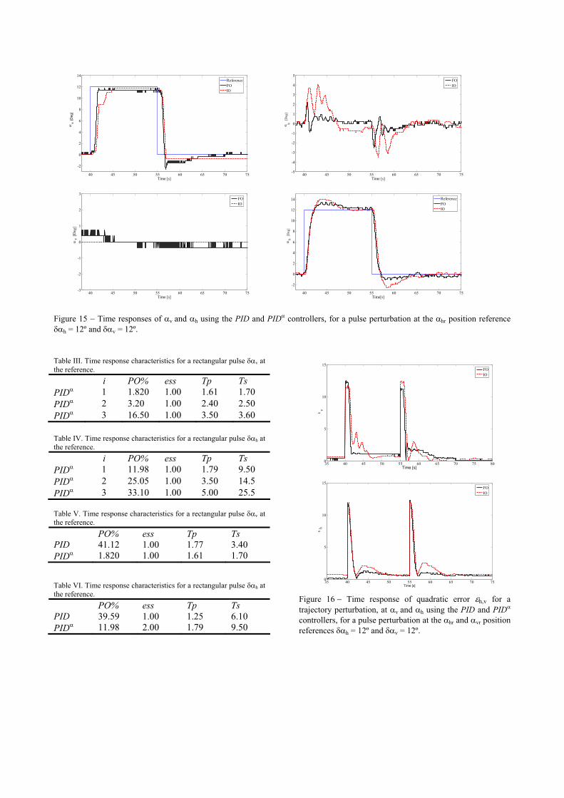
Figure 15 � Time responses of �v and �h using the PID and PID� controllers, for a pulse perturbation at the �hr position reference '�h = 12º and '�v = 12º. Table III. Time response characteristics for a rectangular pulse '�v at the reference. i PO% ess Tp Ts PID� 1 1.820 1.00 1.61 1.70 PID� 2 3.20 1.00 2.40 2.50 PID� 3 16.50 1.00 3.50 3.60 Table IV. Time response characteristics for a rectangular pulse '�h at the reference. i PO% ess Tp Ts PID� 1 11.98 1.00 1.79 9.50 PID� 2 25.05 1.00 3.50 14.5 PID� 3 33.10 1.00 5.00 25.5 Table V. Time response characteristics for a rectangular pulse '�v at the reference. PO% ess Tp Ts PID 41.12 1.00 1.77 3.40 PID� 1.820 1.00 1.61 1.70 Table VI. Time response characteristics for a rectangular pulse '�h at the reference. PO% ess Tp Ts PID 39.59 1.00 1.25 6.10 PID� 11.98 2.00 1.79 9.50

35 40 45 50 55 60 65 70 75 800

5

10

15

*

Time [s]

v

FOIO

35 40 45 50 55 60 65 70 750

5

10

15

Time [s]

*h

FOIO

Figure 16�� Time response of quadratic error *h,v for a trajectory perturbation, at �v and �h using the PID and PID� controllers, for a pulse perturbation at the �hr and �vr position references '�h = 12º and '�v = 12º.

40 45 50 55 60 65 70 75-3

-2

-1

0

1

2

3

Time [s]

Uv

FOIO

Figure 17 � Time response of Uh using the PID and the PID� controllers, for a pulse perturbation at the �hr position reference '�h = 12º.

40 45 50 55 60 65 70 750

0.5

1

1.5

2

2.5

Time [s]

Uh

FOIO

Figure 18 � Time response of Uv using the PID and the PID� controllers, for a pulse perturbation at the �vr position reference '�v = 12º.

0 0.5 1 1.5 2 2.50

200

400

600

800

1000

1200

Uv [V]

Rel

ativ

e Fr

eque

nce

PID

-2.5 -2 -1.5 -1 -0.5 0 0.5 1 1.5 2 2.50

50

100

150

200

250

300

Uh [V]

Rel

ativ

e Fr

eque

nce

PID

Figure 19�� Rotor and tail voltage statistical distributions using the PID, for a pulse perturbation at the position reference '�v = 12º for sampling time h = 0.01s.

0 0.5 1 1.5 2 2.50

50

100

150

200

250

300

350

400

Uv [V]

Rel

ativ

e Fr

eque

nce

PID

-2.5 -2 -1.5 -1 -0.5 0 0.5 1 1.5 2 2.50

50

100

150

200

250

300

350

400

Uh [V]

Rel

ativ

e Fr

eque

nce

PID

Figure 20�� Rotor and tail voltage statistical distributions using the PID, for a pulse perturbation at the position reference '�h = 12º for sampling time h = 0.01s. Table VII. Statistical analysis for a rectangular pulse '�v at the reference. Vv(Mean) Vh(Mean) +v +hPID 1.3353 -0.06 0.4802 0.5800 PID� 1.3200 -0.03 0.5000 0.7491 Table VIII. Statistical analysis for a rectangular pulse '�h at the reference. Vv(Mean) Vh(Mean) +v +hPID 1.300 0.338 0.5900 0.5470 PID� 0.834 0.420 0.0660 0.8386 In the next group of experiments we introduce two different loads at the ends of the beam, under the DC motor, near the main rotor. The two external loads have mass M1 = 0.0149 Kg and M2 = 0.0298 Kg. The maxim use weight capability of the main rotor is 0.150 Kg (tested in the lab with a dynamometer). Figure 21 and 22 show the time responses of �v and Uv for these perturbations.

18 20 22 24 26 28 30 32 34 36 38 40

-14

-12

-10

-8

-6

-4

-2

0

2

Time [s]

v�

IO (M2)

IO (M1)FO (M2)

FO (M1)

Figure 21 � Time response of �v using the PID and the PID� for a external perturbation at the �hr position reference for M1 = 0.0149 Kg and M2 = 0.0298 Kg.

20 25 30 350

0.5

1

1.5

2

2.5

Time [s]

Uv

FO (M1)

IO (M1)

18 20 22 24 26 28 30 32 34 36 38 400.4

0.6

0.8

1

1.2

1.4

1.6

1.8

2

2.2

2.4

Time [s]

Uv

IO (M2)

FO (M2)

Figure 22 � Time response of Uv using the PID and the PID� for a external perturbation at the �hr position reference for M1 = 0.0149 Kg and M2 = 0.0298 Kg We observe that before the external perturbation the consumption of the PID� controller is a reduced amount of energy than the PID to perform the same task. Nevertheless, after the introduction of one perturbation at h = 20 seconds, the main controller needs to compensate the perturbation and in the case of PID� controller requires more energy than the PID.

5. CONCLUSIONS In this paper a two rotor MIMO helicopter system is studied and experimented. The mathematical model of TRMS is derived, and its dynamical characteristics, such as equilibrium position, propeller thrust and gravity compensation are analyzed. For this system are compared integer and fractional order algorithms. The results of the PID� controller reveal better performances than the classical controller. The performances are evaluated by introducing a small perturbation at the reference and an external load perturbation. The results demonstrate a good performance for the PID�� controller. REFERENCES [1] J. Gordon Leishman, Principles of Helicopter Aerodynamics,

Second Edition, Cambridge University Press.

[2] Martin D. Maisel, Demo J. Giulianetti and Daniel C. Dugan, The History of the XV-15 Tilt Rotor Research Aircraft From Concept to Flight, National Aeronautics and Space

Administration Office of Policy and Plans NASA History Division Washington, D.C.2000.

[3] Feedback Instruments Ltd. Manual: 33-007-1C Ed04, 2002.

[4] M. López Martínez, F.R. Rubio (2004), Approximate Feedback Linearization of a Laboratory Helicopter, Sixth Portuguese Conference on Automatic Control, pp.43-45, Faro, Portugal

[5] Islam, B.U.; Ahmed, N.; Bhatti, D.L.; Khan, S., Controller design using fuzzy logic for a twin rotor MIMO system, Multi Topic Conference, 2003. INMIC2003. 7th Internationa,lVolume , Issue , 8-9 Dec. 2003 Page(s): 264 – 268.

[6] Przemys�aw Gorczyca, Krystyn Hajduk, Tracking Control Algorithms For A Laboratory Aerodynamical System, Int. J. Appl. Math. Comput. Sci., 2004, Vol. 14, No. 4, 469–475.

[7] Rahideh, A, Shaheed, M H, Proceedings of the I MECH E Part I Journal of Systems & Control Engineering, Volume 221, Number 1, January 2007 , pp. 89-101(13)

[8] Amaral, T.G.; Crisostomo, M.M.; Pires, V.F., Helicopter motion control using adaptive neuro-fuzzy inference controller, IEEE IECON 02 Volume: 3 , 5-8 Nov. 2002 , Page(s): 2090 -2095 vol.3

[9] Åström, K., Hang, C., Persson, P. and Ho,W. (1992). Towards intelligent PID control, Automática 28(1): 1–9.

[10] Åström, K. J. and Hägglund, T. (1995). PID controller-Theory, Design and Tuning, second edn, Instrument Society of America, 67 Alexander Drive, POBox 12277, Research Triangle Park, North Carolina 27709, USA.

[11] Åström, K. J. and Wittenmark, B. (1984). Computer Controlled Systems, theory and Design, Prentice-Hall, Englewood Cliffs.

[12] Siler, W. and Ying, H. (1989). Fuzzy control theory: The linear case, Fuzzy Sets and Systems 33: 275–290.

[13] Tso, S. K. and Fung, Y. H. (1997). Methodological development of fuzzy-logic controllers from multivariable linear control, IEEE Trans. Systems Man & Cybernetics 27(3): 566–572.

[13] Podlubny, Fractional Differential Equations, Academic Press, San Diego, 1999.

[14] K. S. Miller and B. Ross, An Introduction to the Fractional Calculus and Fractional Differential Equations, Wiley & Sons, New York, 1993.

[15] R. Hilfer, Applications of Fractional Calculus in Physics, World Scientific, Singapore, 2000.

[16] A. Oustaloup, La Commande CRONE: Commande Robuste d'Ordre Non Entier, Editions Hermès, Paris, 1991.

[17] Machado, J. A. T., Discrete-Time Fractional-Order Controllers, FCAA J. of Fractional Calculus & Applied Analysis Vol. 4; pp. 47–66, 2001.