APPLICATION OF ATOMISTIC SCALE SIMULATIONS TO ...

APPLICATION OF ATOMISTIC SCALE SIMULATIONS TO ZIRCONIUM HYDRIDE AND

CARBON-BASED MATERIALS

By

LINYUAN SHI

A DISSERTATION PRESENTED TO THE GRADUATE SCHOOL

OF THE UNIVERSITY OF FLORIDA IN PARTIAL FULFILLMENT

OF THE REQUIREMENTS FOR THE DEGREE OF

DOCTOR OF PHILOSOPHY

UNIVERSITY OF FLORIDA

2021

To my family and friends

4

ACKNOWLEDGMENTS

Although, it is necessarily incomplete to thank people as an acknowledgement, I would

first like to express my sincerest appreciation to my advisor, Prof. Simon R. Phillpot for his

generous support, kindness, and broad knowledge. His serious scientific attitude, rigorous

academic spirit, and excelsior working style have deeply infected and inspired me. His style of

gradual progression towards any problem helps me get through a lot of difficulties in my

graduate journey. I couldn’t have asked for a better advisor than him. Besides my advisor, I

would like to thank Dr. Tonks for his meaningful mentoring and active collaboration. I would

also like to thank the rest of the members of my committee Dr. Spearot and Dr. Sankar for their

insightful suggestions and encouragements.

I would like to extend my thanks to Marina for three years’ collaboration and support.

Moreover, I would like to take this opportunity to thank the past and present members of

FLAMES group, for the insightful discussions and warm friendship. In particular, I would thank

to Dr. Fullarton for her mentoring, kindness, caring attitude and delicious cakes. She gave me

lots of help and instructed me how to use Demeter and HiperGator when I just joined FLAMES

group. I would like to thank Dr. Ragasa for discussions on interesting research ideas and Dr.

Pandey for his optimistic personality, humble attitude and many helps about VASP calculations.

I would also like to thank Ximeng for organizing Hotpot gatherings and other group members for

their meaningful suggestions on my research that created my papers.

Last but not the least, I am forever thankful to my parents for their unconditional support

and endless love. My parents have always supported me every decision and allow me to freely

purse my dreams and life goals. Their constant support is invaluable and precious for me. This

dissertation is dedicated to them for their sacrifices.

5

TABLE OF CONTENTS

page

ACKNOWLEDGMENTS ...............................................................................................................4

LIST OF TABLES ...........................................................................................................................7

LIST OF FIGURES .........................................................................................................................8

LIST OF ABBREVIATIONS ........................................................................................................11

ABSTRACT ...................................................................................................................................12

CHAPTER

1 INTRODUCTION ..................................................................................................................14

1.1 Overview ......................................................................................................................14

1.2 Zirconium-Hydride System .........................................................................................16 1.3 Ablative Materials ........................................................................................................17

2 SIMULATION METHODOLOGY .......................................................................................21

2.1 Overview ......................................................................................................................21 2.2 Density Functional Theory ..........................................................................................22

2.3 Molecular Dynamics ....................................................................................................25 2.3.1 Integration Method ...........................................................................................25

2.3.2 Interatomic Potentials .......................................................................................27 2.3.3 Thermostat ........................................................................................................31

2.3.4 Ensembles .........................................................................................................32

3 NANOINDENTATION OF ZRH2 BY MOLECULAR DYNAMICS SIMULATION ........34

3.1 Background ..................................................................................................................34

3.2 Methods and Simulation Setup ....................................................................................35 3.2.1 Interatomic Potential .........................................................................................35 3.2.2 Simulation Setup...............................................................................................37 3.2.3 Theory and Analysis Method ...........................................................................41

3.3 Analysis of Loading and Unloading ............................................................................44

3.3.1 The Effect of Indenter Speed and Active Layer Thickness ..............................45 3.3.2 Hertz Law and Hardness ...................................................................................47

3.4 Atomic-level Mechanisms ...........................................................................................51 3.4.1 Nanoindentation on the (100) Surface ..............................................................51

3.4.2 Nanoindentation on (110) Surface ....................................................................60 3.5 Summary ......................................................................................................................63

4 GENERATION AND CHARACTERIZATION OF AN IMPROVED CARBON

FIBER MODEL ......................................................................................................................65

6

4.1 Background ..................................................................................................................65 4.2 Simulation and Characterization Methods ...................................................................68

4.2.1 A Brief Introduction to kMC-MD Model .........................................................68 4.2.2 CF Generation Procedure .................................................................................69 4.2.3 Controlling the Shape of CF .............................................................................71 4.2.4 Structural Characterization of Generated CF ...................................................72 4.2.5 Discontinuous CF Model ..................................................................................74

4.3 Microstructure of CF....................................................................................................76 4.3.1 Vacancy Formation Energy ..............................................................................76 4.3.2 Initial Configurations and Snapshots of CF Models ........................................80 4.3.3 Shapes, Densities, and Pores ............................................................................82 4.3.4 Hybridization State of Carbon ..........................................................................85

4.3.5 XRD Analysis ...................................................................................................88

4.3.6 Mechanical Properties ......................................................................................91 4.4 Summary ......................................................................................................................99

5 GENERATION AND CHARACTERIZATION OF AMORPHOUS CARBON USING

A LIQUID QUENCH METHOD .........................................................................................102

5.1 Background ................................................................................................................102 5.2 Computational Methods .............................................................................................103

5.3 Characterization of Amorphous Carbon ....................................................................104 5.4 Summary ....................................................................................................................114

6 SIMULATON OF THE INITIAL STAGE OF HIGH-TEMPERATURE OXIDATION

OF CARBON FIBER AND AMORPHOUS CARBON CHAR ..........................................115

6.1 Background ................................................................................................................115 6.2 Computational Methods .............................................................................................118

6.2.1 Generation of the Carbon Fiber Structure ......................................................118 6.2.2 Generation of the Amorphous Carbon Char Structures..................................119 6.2.3 Overall Simulation Settings ............................................................................121

6.2.4 Reaction Parameter Analysis ..........................................................................123 6.2.5 Oxygen Adsorption on Surface ......................................................................127

6.3 Results and Discussion ..............................................................................................130

6.3.1 Analysis of the Oxidation of Carbon Fiber ....................................................130 6.3.2 Oxidation of Amorphous Carbon ...................................................................138

6.4 Summary ....................................................................................................................145

7 SUMMARY AND CONCLUSION .....................................................................................147

LIST OF REFERENCES .............................................................................................................151

BIOGRAPHICAL SKETCH .......................................................................................................165

7

LIST OF TABLES

Table page

3-1 Lattice parameter, elastic constants, and moduli of cubic fluorite ZrH2 calculated by

DFT and COMB3 potential. ..............................................................................................37

3-2 Young’s modulus, Poisson’s ratio, and reduced Young’s modulus of δ-ZrH2 in the

[100] and [110] orientations obtained from the COMB3 potential. ..................................43

3-3 The fitted reduced Young’s modulus of δ-ZrH2 obtained from the load vs. force

curves of various thickness of active layers in the [100] and [110] orientations. ..............49

4-1 Densities, number of atoms and system size of the initial system used in the

generation of CFs as well as the corresponding CF type.. .................................................80

4-2 Average crystallite size of fiber cores and thin fibers for various initial densities. ...........91

4-3 The tensile moduli of continuous and discontinuous fiber core and thin fibers

predicted from the tensile simulation .................................................................................95

5-1 The comparison of final sp2 and sp3 content of amorphous carbon structures using

ReaxFF and REBO potentials for various densities from this work and

Ranganathan’s work[141]. ...............................................................................................107

5-2 List of values of peak (P) and its positions (R) of pair correlation functions of

amorphous carbon structures for various densities using REBO and ReaxFF

potentials ..........................................................................................................................113

6-1 Reaction rate fitting model ...............................................................................................125

6-2 The activation energy of reactions fitted from model 1 to model 6 and the prediction

error of each model for the oxidation of CFs. ..................................................................137

6-3 The activation energy of reactions fitted from model 1 to model 6 and the prediction

error of each model for the oxidation of amorphous carbon char. ...................................144

8

LIST OF FIGURES

Figure page

1-1 Illustration of the phenomenology of porous ablative materials[20] .................................19

3-1 Sketch of the simulation system for nanoindentation on ZrH2. .........................................39

3-2 The unit cell and conventional cell of ẟ-ZrH2 ....................................................................41

3-3 The force vs. indentation depth curves with different settings. .........................................47

3-4 Force vs. ℎ3/2 for active layers of different thickness .......................................................49

3-5 Hardness vs. indentation depth with active layers of different thickness ..........................51

3-6 Dimensionless load vs. indentation depth and hardness vs. indentation depth. ................51

3-7 The indentation force vs. depth curves and simulation snapshots at different depth. .......54

3-8 The snapshots of the final dislocations after unloading with different indentation

depth. ..................................................................................................................................55

3-9 Snapshots of the dislocations before and after the yielding point for the

nanoindentation on the (100) surface. ................................................................................57

3-10 Selected snapshots of δ-ZrH2 at different indentation depths from a 3D perspective .......59

3-11 Selected snapshots of δ-ZrH2 at an indentation depth of 20Å and 25Å from a 3D

perspective during nanoindentation simulations for the [100] orientation. .......................59

3-12 The selected snapshots of δ-ZrH2 at different indentation depths from a 3D

perspective during nanoindentation simulations for the [110] orientation ........................62

3-13 Cross section of δ-ZrH2 at an indentation depth of 25Å during simulations for the

[110] orientation.................................................................................................................63

4-1 Top view of the initial system packed with ladder structures. ...........................................69

4-2 Top view of initial and final structures of thin fiber ..........................................................72

4-3 Illustrations of surface mesh method on thin fiber volume calculation. ............................74

4-4 Illustrions of discontinuous fiber model ............................................................................76

4-5 The lattice of graphite crystal ............................................................................................78

4-6 Single vacancy formation energy of graphite ....................................................................79

https://uflorida-my.sharepoint.com/personal/sly1993_ufl_edu/Documents/Research/Dissertation/Dissertation_V5.docx#_Toc64294699

https://uflorida-my.sharepoint.com/personal/sly1993_ufl_edu/Documents/Research/Dissertation/Dissertation_V5.docx#_Toc64294699

9

4-7 Averaged vacancy formation energy when 1, 2 or 3 carbon atoms are removed from

the lattice ............................................................................................................................79

4-8 Atomistic snapshots of fiber core and thin fiber microstructures after bond formation

cycles and ReaxFF relaxation with various initial densities from 1.2 g/cm3 to 2.0

g/cm3 ..................................................................................................................................81

4-9 The initial and final densities of fiber core and thin fibers after NPT relaxation with

ReaxFF potential ................................................................................................................83

4-10 Pore size distribution of fiber cores and thin fibers for various initial densities

ranging from 1.2-2.0 g/cm3 ................................................................................................84

4-11 Total volume fraction of pores of fiber microstructures for various initial densities

ranging from 1.2-2.0 g/cm3 after bond formation (dash lines) and NPT relaxations

(solid lines).........................................................................................................................85

4-12 Evolution of carbon sp and sp2 hybridization content for fiber cores with various

initial densities ...................................................................................................................87

4-13 Virtual XRD patterns of fiber core microstructures ..........................................................89

4-14 The changes of gap width of fiber core microstructure during pre-relaxation and

tensile simulation ...............................................................................................................94

4-15 Stress-strain curved predicted in tensile simulation of CF sample for various initial

densities and the snapshots of 1.8 g/cm3 samples at yield points ......................................96

4-16 The transverse moduli of fiber core models ......................................................................99

5-1 Snapshots of amorphous carbon at various densities from 0.5 g/cm3 to 3.2 g/cm3

using the REBO potential ................................................................................................106

5-2 Atomistic snapshots of amorphous carbon at various density from 0.5 g/cm3 to 2.0

g/cm3 using the ReaxFF potential. ...................................................................................106

5-3 The final hybridization content for amorphous carbon structure for various densities

using REBO and ReaxFF potentials, respectively. ..........................................................108

5-4 The carbon hybridization content for various densities during the liquid quench

process using the REBO potential. ..................................................................................109

5-5 The carbon hybridization content for various densities during the liquid quench

process using ReaxFF potential .......................................................................................110

5-6 Structural characterization of amorphous carbon structures of various densities using

REBO and ReaxFF potentials. .........................................................................................112

10

5-7 The pore size distributions of amorphous carbon structures for various densities

using REBO and ReaxFF potentials, respectively. ..........................................................113

6-1 The snapshots of generated amorphous carbon char .......................................................120

6-2 The snapshots of fiber and char models after oxygen insertion .......................................123

6-3 The predictive curve of species fitted to model 6 and the data obtained from the MD

simulation from the oxidation simulation of CF under 3500K. .......................................127

6-4 The snapshots of oxygen adsorption on the surfaces of fiber and amorphous char ........129

6-5 The average lifetime (blue bar) and occurrences (orange line) of O, O2, CO, CO2, C2O and Os at from 1000 K to 4500 K during the oxidation simulation of CF ...............132

6-6 The lifetime distribution of atomic oxygen at different temperatures from 1000 K to

4500 K and fitted by the gaussian kernel density estimation (blue line) .........................134

6-7 The concentration of O, O2, CO, CO2, Os and (Os+O) as function of time during the

oxidation simulation.........................................................................................................135

6-8 Logarithm of the reaction rate against the inverse temperature for different reactions

for the oxidation of CF .....................................................................................................137

6-9 The predicted concentration of O, Os and CO for CF as function of time by model 4

for the oxidation of CF .....................................................................................................138

6-10 The average lifetime (blue bar) and occurrences (orange line) of O, O2, CO, CO2, C2O and Os at from 1000 K to 4500 K during the oxidation simulation of amorphous

carbon char .......................................................................................................................140

6-11 The concentration of O, O2, CO, CO2, Os and (Os+O) as function of time during the

oxidation simulation.........................................................................................................142

6-12 Logarithm of the reaction rate against the inverse temperature for different reactions

for the oxidation of amorphous carbon char ....................................................................144

6-13 The predicted concentration of O, Os and CO for CF as function of time by model 4

for the oxidation of amorphous carbon char ....................................................................145

11

LIST OF ABBREVIATIONS

CF Carbon Fiber

COMB Charge-Optimized Many Body

DFT Density Functional Theory

GGA Generalized Gradient Approximation

kMC Kinetic Monte Carlo

LDA Local Density Approximation

LJ Lenard-Jones

MD Molecular Dynamics

ReaxFF Reactive Force Field

12

Abstract of Dissertation Presented to the Graduate School

of the University of Florida in Partial Fulfillment of the

Requirements for the Degree of Doctor of Philosophy

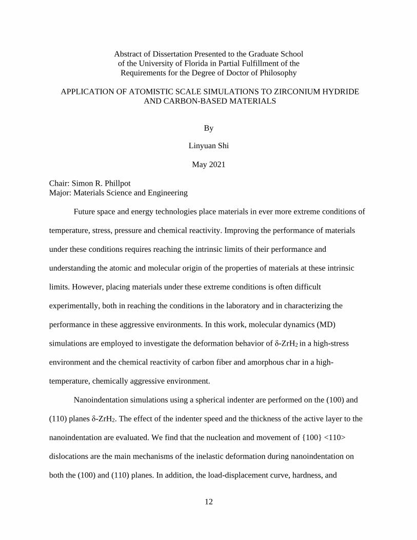
APPLICATION OF ATOMISTIC SCALE SIMULATIONS TO ZIRCONIUM HYDRIDE

AND CARBON-BASED MATERIALS

By

Linyuan Shi

May 2021

Chair: Simon R. Phillpot

Major: Materials Science and Engineering

Future space and energy technologies place materials in ever more extreme conditions of

temperature, stress, pressure and chemical reactivity. Improving the performance of materials

under these conditions requires reaching the intrinsic limits of their performance and

understanding the atomic and molecular origin of the properties of materials at these intrinsic

limits. However, placing materials under these extreme conditions is often difficult

experimentally, both in reaching the conditions in the laboratory and in characterizing the

performance in these aggressive environments. In this work, molecular dynamics (MD)

simulations are employed to investigate the deformation behavior of ẟ-ZrH2 in a high-stress

environment and the chemical reactivity of carbon fiber and amorphous char in a high-

temperature, chemically aggressive environment.

Nanoindentation simulations using a spherical indenter are performed on the (100) and

(110) planes ẟ-ZrH2. The effect of the indenter speed and the thickness of the active layer to the

nanoindentation are evaluated. We find that the nucleation and movement of {100} <110>

dislocations are the main mechanisms of the inelastic deformation during nanoindentation on

both the (100) and (110) planes. In addition, the load-displacement curve, hardness, and

13

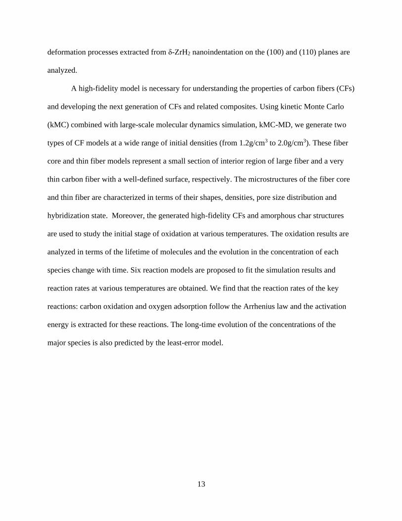
deformation processes extracted from δ-ZrH2 nanoindentation on the (100) and (110) planes are

analyzed.

A high-fidelity model is necessary for understanding the properties of carbon fibers (CFs)

and developing the next generation of CFs and related composites. Using kinetic Monte Carlo

(kMC) combined with large-scale molecular dynamics simulation, kMC-MD, we generate two

types of CF models at a wide range of initial densities (from 1.2g/cm3 to 2.0g/cm3). These fiber

core and thin fiber models represent a small section of interior region of large fiber and a very

thin carbon fiber with a well-defined surface, respectively. The microstructures of the fiber core

and thin fiber are characterized in terms of their shapes, densities, pore size distribution and

hybridization state. Moreover, the generated high-fidelity CFs and amorphous char structures

are used to study the initial stage of oxidation at various temperatures. The oxidation results are

analyzed in terms of the lifetime of molecules and the evolution in the concentration of each

species change with time. Six reaction models are proposed to fit the simulation results and

reaction rates at various temperatures are obtained. We find that the reaction rates of the key

reactions: carbon oxidation and oxygen adsorption follow the Arrhenius law and the activation

energy is extracted for these reactions. The long-time evolution of the concentrations of the

major species is also predicted by the least-error model.

14

CHAPTER 1

INTRODUCTION

1.1 Overview

Future space and energy technologies place increasing demands on the materials

performance through severe conditions, such as high temperature, high stress and pressure,

chemically highly reactive environments, and high radiation environments. For example, next-

generation nuclear reactors require materials to function in highly corrosive resistance for a long

period of time without failure.[1] Space vehicles requires outer surface coating materials capable

of withstanding higher temperatures and preventing overheating of the vehicle and its payload,

including astronauts. These environments require reaching ever closer to the intrinsic limit of

materials performance and better understanding the atomic and molecular origin of failure of

materials at this intrinsic limit. However, it is often difficult to reproduce these extreme

conditions in experiment; moreover, it can also be difficult to instrument experiments for such

aggressive conditions. Over the last few decades, advancements in computer technology have

reached an impressive level.[2] With the help of the increasing computer power, physics-based

computational modeling has been widely used as a complementary approach for industry and

academia to predict the properties of materials and to probe physical systems. Such modeling is

now a fundamental tool for all disciplines, including Materials Science.[3] Computational

models now have the ability to elucidate the key physical mechanisms from atomic to

macroscopic dimensions that materials are subject to in these extreme environment affect

materials. These behaviors can even result in failure of the material. An understanding of these

processes is a prerequisite for ultimately enabling the atomic or molecular structure of materials

to be manipulated or adjusted in a predicable manner to create new material and microstructures

with extraordinary tolerance to harsh environments. In this work, Molecular Dynamics (MD)

15

simulation is used to investigate zirconium hydride and carbon-based fiber systems and to

develop an understanding of the kinetic processes within these systems within the harsh

environments of high temperature and high stress (ZrH2) and high temperature and high

chemical reactivity (carbon fiber).

MD is a classical computation approach to study the temporal evolution of systems of

large numbers of atoms.[4] By analyzing the trajectories of atoms and assessing numerous time-

dependent observables of the complex system, MD can predict the mechanical, thermodynamic

and chemical properties of materials as function of time. Compared with first principles-based

methods, such as density functional theory, MD is capable of simulating much larger, and

complex dynamic systems at the atomic scale, albeit typically with the sacrifice of the materials

fidelity of the simulation. Moreover, the mechanisms and key parameters that can be extracted

from MD simulations can serve as a foundation for mesoscale and macroscale computational

methods such as phase field and finite element methods.

In this work, MD is used to generate high-fidelity models, predict structural properties of

crystal and amorphous structures, compute mechanical properties such as elastic constants, and

characterize complex chemistry, such as reaction rates and the evolution of species as a function

of time in the simulation. Specifically, MD is used to (1) evaluate the mechanical properties of

the zirconium hydride system, to investigate the dislocation mechanism of the nanoindentation of

ZrH2, and (2) to generate the high-fidelity models, characterize the structural properties and

simulate the initial stage of the oxidation processes of carbon fiber (CF) and amorphous carbon

systems.

16

1.2 Zirconium-Hydride System

Zirconium alloys such as Zircaloy have been commonly used as fuel cladding in the light

water reactors as they exhibit high temperature corrosion resistance and low thermal neutron

capture cross-section.[5] Despite the high temperature corrosion resistance, Zr alloys experience

a slow corrosion process in which they are oxidized by the coolant water on the outer surface of

the fuel cladding. Hydrogen (H2) is produced in this slow oxidation process and then diffuses

into the zirconium alloy component. The total hydrogen concentration in the cladding gradually

increases from the initial average value of ~3 wt parts per million (wppm) to high values as 600-

700 wppm in this process. [6] Zirconium hydride precipitates in the Zircaloy cladding once the

hydrogen concentration exceeds the solubility limit. The presence of zirconium hydride

significantly degrades the performance of cladding, lowers its ductility and embrittles the

material. Moreover, the inhomogeneous distribution of the zirconium hydride stresses the

degradation of the material. The detrimental effects of zirconium hydride and the associated

microstructure changes impact the safety and long-term reliability of the cladding. It is critical to

understand the mechanisms of the deformation and fracture in zirconium hydride to ensure the

safe application of these alloys for cladding applications.

Zirconium hydride has been extensively studied and simulated at the atomistic scale[7–

12] and it forms various phases, depending on the ratio between the Zr and H atoms in the lattice.

The properties of the Zr-H system, such as unstable stacking energy, surface energy and interface

energy, have been extensively studied via first principles methods. The effect of hydrogen on the

crack growth in 𝛼- zirconium has been modeled by molecular dynamics. [13] These simulations

show that zirconium hydride is a brittle phase in the zirconium matrix that results the reduction

of the ductility of zirconium alloys. However, little work[14,15] has been carried out to

17

investigate and understand the plastic deformation of zirconium hydride, which is not

straightforward to probe experimentally. Therefore, understanding and accurately modeling the

deformation behaviors of the Zr-H especially for the common 𝛿- ZrH2 phase is critical to

improve the performance of the fuel cladding. MD simulations can help us to develop a better

understanding of and to predict the deformation behaviors of nuclear fuel cladding from the

atomistic view. Therefore, the mechanical properties and the deformation behavior of 𝛿- ZrH2 is

studied in this dissertation.

1.3 Ablative Materials

Ablative materials are widely used as an important part of thermal protection system

(TPS) in spacecraft[16–18]. Specifically, they act maintain the integrity of the vehicles and the

safety of payload inside the spacecraft, including astronauts, from the excessive heating during

the atmospheric entry process. Specifically, the ablative materials can absorb heat through

endothermic pyrolysis of the substrate. Phenolic Impregnated Carbon Ablator (PICA)[19], a

carbon reinforced composites with a phenolic resin matrix, is a typical carbon-based ablative

material. Because of the sacrificial nature of the PICA, minimizing the thickness of the ablator

will reduce the weight of the space vehicle and improve its performance. The post-analysis of the

Stardust flight data[17] showed that the actual recession depth of the TPS was 20-60% lower

than predicted. Therefore, it is essential to understand the mechanism in the pyrolysis and

improve the accuracy of prediction.

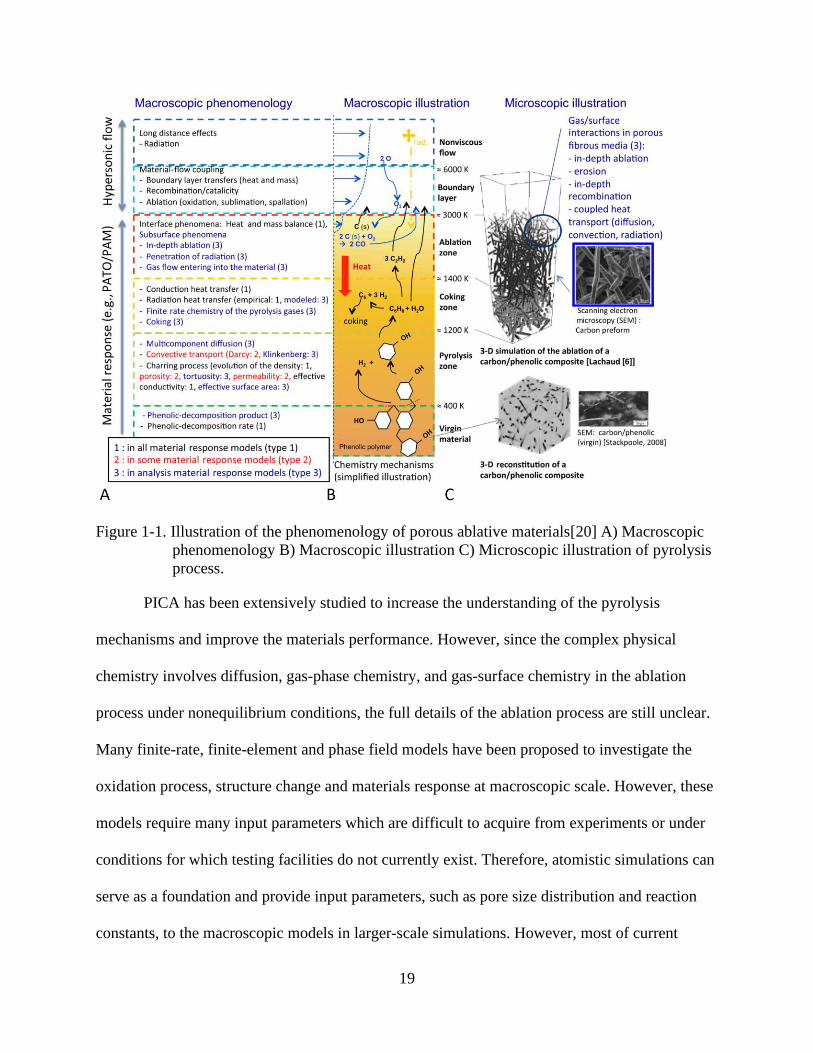
Figure 1-1 A. and B. illustrates the general gas-chemistry phenomena that occur in the

materials response of PICA during the atmospheric entry. Virgin materials experience thermal

degradation and surface recession, captured by the solid pyrolysis, gas transport and ablation

chemistry. The phenolic resin thermally decomposes and carbonizes into a low-density

18

turbostratic graphite in the pyrolysis zone. During the decomposition process, the resin loses

mass and releases the pyrolysis gas, which is a mixture of water, hydrogen and

hydrocarbons.[20] Phenol and hydrogen are the principle products in the pyrolysis The pyrolysis

gases transport and diffuse into the surfaces through the porous microstructures in the coking and

ablation zones. A char can be produced in the pyrolysis gas mixture with possible coking effects

by the homogenous and heterogenous reactions. Meanwhile, the char can be oxidized to CO and

re-transformed into the pyrolysis gas. In the ablation zone, materials are removed, and the

surface recedes due to the ablation. Depending on the conditions of atmospheric entry, the

ablation can be caused by the mechanical erosion, phase changes and heterogeneous reactions.

Figure 1-1 C. shows the structure evolution of the carbon fiber and the matrix in the ablation

from the microscopic view. During the entry process, the resin is gradually charred, and the

carbon fiber is pitted and attacked by the pyrolysis gas. The resin matrix at outer surface is

eliminated and transformed into the gas mixture and only carbon fiber is left near the surface,

where the carbon atoms in the fiber can be oxidized to CO.

19

Figure 1-1. Illustration of the phenomenology of porous ablative materials[20] A) Macroscopic

phenomenology B) Macroscopic illustration C) Microscopic illustration of pyrolysis

process.

PICA has been extensively studied to increase the understanding of the pyrolysis

mechanisms and improve the materials performance. However, since the complex physical

chemistry involves diffusion, gas-phase chemistry, and gas-surface chemistry in the ablation

process under nonequilibrium conditions, the full details of the ablation process are still unclear.

Many finite-rate, finite-element and phase field models have been proposed to investigate the

oxidation process, structure change and materials response at macroscopic scale. However, these

models require many input parameters which are difficult to acquire from experiments or under

conditions for which testing facilities do not currently exist. Therefore, atomistic simulations can

serve as a foundation and provide input parameters, such as pore size distribution and reaction

constants, to the macroscopic models in larger-scale simulations. However, most of current

20

atomistic simulations focus on the simulation of the pyrolysis of resin by DFT and MD methods.

Although fiber and char are important in the ablation process of PICA, because of their

complicated microstructure, little work has been done on the properties of them at atomistic

scale. Moreover, the complicated characterization process and lengthy pre- and post- data

processing increases the difficulty of analyzing the simulations. In this dissertation, high-fidelity

carbon fiber and char models are generated at atomistic scale to address the issue of the

representation of the microstructure. With the help of Ovito software[21] and python scripts,

advanced characterization methods are employed to characterize the structural properties and

investigate the oxidation process of carbon fiber and char. The proposed high-fidelity models can

be used to investigate the composites of polymer and carbon/char. Moreover, the mechanisms

and parameters obtained from the simulations of fiber and char in this work can be utilized by

mesoscale models to predict the ablation behavior of PICA.

21

CHAPTER 2

SIMULATION METHODOLOGY

2.1 Overview

Atomic scale simulations provide fundamental insights and understanding of materials

behavior and properties across length scales from Angstroms to hundreds of nanometers. In

general, compared with experiments, simulation and modeling analysis is cheap and timesaving;

therefore, simulation analysis of materials is widely favored by both academia and industry. Ab-

initio methods, such as Density Functional Theory (DFT), and classical methods, such as

Molecular Dynamics (MD), are widely employed in atomic scale simulations. Ab-initio methods

use quantum-mechanical models to describe the interaction between particles including nuclei

and electrons, while empirical potentials use analytic functional forms to describe interactions

between atoms. Ab-initio method can be used to investigate the optical, electronic, and magnetic

properties of materials. However, the size of the material systems that can be investigated by ab-

initio method is limited to a maximum of only about 500 atoms because of the complexity of the

quantum mechanical description. Unlike the ab-initio methods, classical methods are capable of

modeling dynamical processes in relatively large systems, millions of atoms or more, over a time

span from picoseconds to nanoseconds. These larger system sizes and long times are possible

because the contribution of electrons to the interaction is ignored at the cost of materials fidelity.

In this dissertation, density functional theory (DFT) and molecular dynamics (MD) are

both employed to investigate the microstructure, dynamics, and physical and chemical

phenomenon in zirconium hydride and carbon-based systems including carbon fibers (CFs) and

char. The following sections gives a brief introduction of each method employed in this work

and their key concepts.

22

2.2 Density Functional Theory

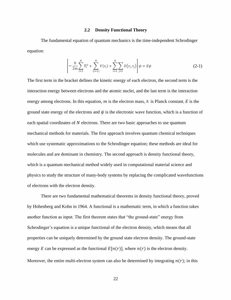
The fundamental equation of quantum mechanics is the time-independent Schrodinger

equation:

[−ℏ

2𝑚∑ 𝛻𝑖

2

𝑁

𝑖=1

+ ∑ 𝑉(𝑟𝑖)

𝑁

{𝑖=1}

+ ∑ ∑ 𝑈(𝑟𝑖 , 𝑟𝑗)

𝑗<𝑖

𝑁

𝑖=1

] 𝜓 = 𝐸𝜓 (2-1)

The first term in the bracket defines the kinetic energy of each electron, the second term is the

interaction energy between electrons and the atomic nuclei, and the last term is the interaction

energy among electrons. In this equation, 𝑚 is the electron mass, ℏ is Planck constant, 𝐸 is the

ground state energy of the electrons and 𝜓 is the electronic wave function, which is a function of

each spatial coordinates of 𝑁 electrons. There are two basic approaches to use quantum

mechanical methods for materials. The first approach involves quantum chemical techniques

which use systematic approximations to the Schrodinger equation; these methods are ideal for

molecules and are dominant in chemistry. The second approach is density functional theory,

which is a quantum mechanical method widely used in computational material science and

physics to study the structure of many-body systems by replacing the complicated wavefunctions

of electrons with the electron density.

There are two fundamental mathematical theorems in density functional theory, proved

by Hohenberg and Kohn in 1964. A functional is a mathematic term, in which a function takes

another function as input. The first theorem states that “the ground-state” energy from

Schrodinger’s equation is a unique functional of the electron density, which means that all

properties can be uniquely determined by the ground state electron density. The ground-state

energy 𝐸 can be expressed as the functional 𝐸[𝑛(𝑟)], where 𝑛(𝑟) is the electron density.

Moreover, the entire multi-electron system can also be determined by integrating 𝑛(𝑟); in this

23

way the Hamiltonian of the system (including the kinetic energy of the electrons, the interaction

potential energy between the electrons, and the interaction between the external potential field

and the electrons) are also defined. Thereby, all ground state properties of the system are

determined, including total energy, ground state wave function, nth excited energy level, and

indirectly obtainable properties, such as the elastic behavior.

The second theorem is that the electron density that minimizes the energy of the overall

functional is the true electron density corresponding to the full solution of the Schrodinger

equation. This theorem implies that the true electron density is the ground state electron density,

from which the ground state energy can be obtained. In other words, if the true functional form

were known, the relevant electron density could be approached by varying the electron density

until the functional was minimized. The biggest improvement of approaches based on the

Hohenberg-Kohn theorems over the Schrodinger Equation is that the energy can be written in the

functional form of density instead of trying to solve the complicated electronic many-body wave

function.

Although the first Hohenberg-Kohn theorem proves the ground state energy is a unique

functional of electron density, it still cannot be applied in real calculations since the functional

form 𝐸[𝑛(𝑟)] is unknown. One year later, with the proposition of Kohn-Sham equation, DFT

began to be applied in real calculations. The Kohn-Sham equation is expressed as:

[−ℏ

2m∇2 + 𝑉(𝑟) + 𝑉𝐻(𝑟) + 𝑉𝑋𝐶(𝑟)] 𝜓 = 휀𝑖𝜓 (2-2)

where 휀𝑖 is the orbital energy of the corresponding Kohn-Sham orbital and 𝑉(𝑟), 𝑉𝐻(𝑟) and

𝑉𝑋𝐶(𝑟) are three potentials. 𝑉(𝑟) defines the interaction between the collection of nuclei and an

electron which also appeared in the Schrodinger Equation, Eq. 2-1. 𝑉𝐻(𝑟) is the Hartree

potential, which describes the Coulomb repulsion between one electron considered in Eq. 2-2

24

and total electron density. It should be noted that 𝑉𝐻(𝑟) includes the unphysical self-interaction

since the electron considered in the Eq. 2-1 is also the part of the total electron density. This self-

interaction is corrected in 𝑉𝑋𝐶(𝑟), which also defines the exchange and correlation contributions

to the single electron.

The Kohn-Sham equation simplifies the N electron many-body problem into the problem

of solving a single-particle Schrodinger-like equation. The Kohn-Sham equation can be solved

by the algorithm briefly described as following: first, make an initial guess of the electron

density. The single-particle wave function can be obtained by using this trial electron density.

Then the electron density can be calculated by the Kohn-Sham single particle wave function:

𝑛(𝑟) = 2∑𝜓∗𝜓 (2-3)

where 𝜓∗ is the complex conjugate of 𝜓. After this step, the calculated electron density 𝑛(𝑟) is

compared with the initial guess of the electron density. If appropriate, previously defined

convergence criteria are not reached, the initial guess of electron density is updated in some way

and the new wave function is be computed again. This iteration process continues until the

convergence criteria are satisfied.

Since the true form of the exchange-correlation functional is not given by the Hohenberg-

Kohn theorem, Kohn and Sham proposed the local density approximation (LDA) at the same

time as the Kohn-Sham equation. LDA uses a piece-wise uniform electron density function to

define the non-uniform exchange-correlation functional. Although the functional form of LDA is

relatively simple, LDA has achieved great success in the field of electronic structure

computation. In practice, however, it also has a number of failings: most notably, it typically

provides an overestimate of the cohesive energy and underestimate of the lattice parameter.

Another slightly more sophisticated functional, known as generalized gradient approximation

25

(GGA), was proposed after LDA, aiming to be more accurate for calculation. Two widely used

GGA functional are the Perdew-Burke-Ernzerhof functional (PBE) and Perdew-Wang functional

(PW91).

2.3 Molecular Dynamics

Molecular dynamics is a material calculation method by solving Newton’s Equation of

motion:

𝒇𝑖 = 𝒎𝑖

𝑑𝒓𝑖

𝑑𝑡= −

𝜕𝑈

𝜕𝒓𝑖 (2-4)

where 𝒇𝑖 is the force acting on the atom 𝑖, 𝑚𝑖 is the mass, 𝒓𝑖 is the position of atom 𝑖 and 𝑈 is

the potential energy of the system. Through the integration of the equations of motion of the

molecules and atoms, the behavior of the system over time can be investigated from a dynamical

perspective.

2.3.1 Integration Method

Since the form of the potential energy 𝑈(𝒓1, 𝒓2, … , 𝒓𝑁) is complicated and the number of

atoms can be large (up to 106 ~ 108), Newton’s equation (Eq. 2-4) cannot be integrated in time

analytically. With the development of computer technology, we can integrate Newton’s equation

of motion using numerical methods. The position and velocity at the next time step are predicted

by Taylor series expansion of the position at the current time step:

𝒓𝒊(𝑡 + ∆𝑡) = 𝒓𝒊(𝑡) + 𝒗𝒊(𝑡)∆𝑡 +1

2∆𝑡2𝒂(𝑡) +

∆𝑡3

3!

𝑑𝒓𝑖

𝑑𝑡3+ 𝑂(∆𝑡4) (2-5)

Similarly:

𝒓𝒊(𝑡 − ∆𝑡) = 𝒓𝒊(𝑡) − 𝒗𝒊(𝑡)∆𝑡 +1

2∆𝑡2𝒂(𝑡) −

∆𝑡3

3!

𝑑𝒓𝑖

𝑑𝑡3+ 𝑂(∆𝑡4) (2-6)

where 𝒂 is the acceleration of atom 𝑖 at time 𝑡. Adding equation 2-5 and 2-6 together:

𝒓(𝑡 + ∆𝑡) + 𝒓(𝑡 − ∆𝑡) = 2𝒓(𝑡) + ∆𝑡2𝒂(𝑡) + 𝑂(∆𝑡4) (2-7)

26

Move 𝒓(𝑡 − ∆𝑡) to the right side and discard the higher order quadratic term 𝑂(∆𝑡4) yields:

𝒓(𝑡 + ∆𝑡) = 2𝒓(𝑡) − 𝒓(𝑡 − ∆𝑡) + ∆𝑡2𝒂(𝑡) (2-8)

the error of the estimation to the position at next time step is 𝑂(∆𝑡4), where ∆𝑡 is the time step of

the simulation. Therefore, in general, decreasing time step increases the accuracy of the

simulation at the expense of increased computation cost. For metallic materials, the time step is

typically about 1fs. The velocity at time 𝑡 can be obtained by:

𝐯(t) =𝒓(𝑡 + ∆𝑡) − 𝒓(𝑡 − ∆𝑡)

2∆𝑡 (2-9)

and the error of 𝑣(𝑡) is Δ𝑡2. Based on this method, Swope et al.[22,23] proposed an improved

method for the time discretization of Newton’s equations, named the Verlet algorithm. There are

several equivalent variants of the Verlet method. One frequently used form is the so-called

leapfrog scheme where the velocity is calculated at 𝑡 +1

2Δ𝑡 to improve the accuracy of the

calculation. The velocity 𝒗(𝑡 +1

2Δ𝑡) is computed from the velocity 𝒗(𝑡 −

1

2Δ𝑡) and the force

𝑭(𝑡) is computed at time 𝑡:

𝒗 (𝑡 +1

2∆𝑡) = 𝒗 (𝑡 −

1

2Δ𝑡) +

𝑭

𝑚Δ𝑡 (2-10)

The position 𝒓(𝑡 + Δ𝑡) is determined as:

𝒓(𝑡 + ∆𝑡) = 𝒓(𝑡) + 𝒗 (𝑡 +1

2∆𝑡) Δ𝑡 (2-11)

which involves the position 𝒓 at time 𝑡 and the velocity 𝒗 (𝑡 +1

2∆𝑡). It should be noted that the

velocity and position are computed at different times, which reduces the rounding errors. We can

compute the force, velocity, and position of atom by above equations. In general, the rest of the

dynamical properties of this system can be deduced by these three variables. For example, the

pressure of this system can be calculated by:

27

𝑃 =𝑁𝑘𝐵𝑇

𝑉+

1

3𝑉∑ 𝒓𝒊 ⋅ 𝑭𝒊

𝑖

(2-12)

where 𝑃 is pressure, 𝑘𝐵 is Boltzmann constant, 𝑁 is the number of atoms, 𝑇 is the temperature of

system and 𝑉 is the volume of the simulation system. Specially, the temperature 𝑇 of the system

can be calculated by:

𝑇 = ∑𝑚𝑖𝑣𝑖

2

𝑘𝐵𝑁𝑓𝑖

(2-13)

where 𝑁𝑓 is the number of degrees of freedom of the system.

2.3.2 Interatomic Potentials

The time-dependent self-consistent field approach introduced by Dirac shows that the

motion of nuclei is associated to equation 2-14:

𝑚��(𝑡) = −∇𝐑𝑈𝑒𝐸ℎ𝑟(𝑹) (2-14)

where 𝑈𝑒𝐸ℎ𝑟(𝑹) is Ehrenfest potential. Ehrenfest determined that the potential energy 𝑈𝑒

𝐸ℎ𝑟(𝑹)

on a single hypersurface is the potential energy 𝑈0(𝑹) of the stationary electronic Schrodinger

equation for the ground state, where 𝑹 is the coordinates of the nuclei. Since 𝑈𝑒𝐸ℎ𝑟(𝑹) is a

function of coordinates, the classical approach can be derived if we can solve the stationary

electronic Schrodinger equation for a given coordinates configuration. First, the function

𝑈𝑒𝐸ℎ𝑟(𝑹) at a number of points can be evaluated and we then can get data points (𝑹, 𝑈𝑒

𝐸ℎ𝑟(𝑹)).

Second, the global potential energy hypersurface can be approximately reconstructed from these

data points. Therefore, an approximate potential hypersurface can be estimated as an analytical

many-body potential form with a truncation:

𝑈𝑒𝐸ℎ𝑟(𝑹) ≈ 𝑈𝑒

𝑎𝑝𝑝𝑟(𝑹) = ∑ 𝑈1𝑖 (𝑹𝒊) + ∑ 𝑈2𝑖,𝑗 (𝑹𝒊, 𝑹𝒋) + ∑ 𝑈3𝑖,𝑗,𝑘 (𝑹𝒊, 𝑹𝒋, 𝑹𝒌) … (2-15)

28

When the interaction potential is determined, the motion of the nuclei can be evaluated by

replacing 𝑈𝑒𝐸ℎ𝑟(𝑹) with 𝑈𝑒

𝑎𝑝𝑝𝑟(𝑹). Since it’s a drastic approximation from 𝑈𝑒𝐸ℎ𝑟(𝑹) to

𝑈𝑒𝑎𝑝𝑝𝑟(𝑹), the analytic form and its parameters of 𝑈𝑒

𝑎𝑝𝑝𝑟(𝑹) plays a decisive role on the

accuracy of the potential hypersurface and the subsequent estimation of the nuclei motion.

Moreover, quantum mechanical effects are ignored in this approach. However, this method has

been proven successful especially for the calculation of macroscopic properties. The construction

of potential 𝑈𝑒𝑎𝑝𝑝𝑟(𝑹) is a challenging and requires much intuition, hard work and skill.

However, with the development of machine learning, scientists can now train a neural network to

fit a potential automatically with the data acquired form DFT, quantum Monte-Carlo or ab-initio

MD computations. In this dissertation, a simple Lennard-Jones 9-3 potential, a Dreiding

potential, a Reactive Force Field (ReaxFF) and a Charge-Optimized Many Body (COMB)

potential are used. The Lennard-Jones potential is used during the simulation of the

graphitization process of the generation of CF model. The classical Dreiding potential is used to

describe the interactions between ladder units in the CF. The ReaxFF potential is used to model

the oxidation of CF and char, which can describe the bonded system of various elements within a

unified framework. The COMB potential is used to describe the Zr-H system which consists of

both metallic and ionic bonding.

2.3.2.1 Lennard-Jones potential

Lennard-Jones (LJ) potential is a simple intermolecular potential which models the

repulsive and attractive forces. The related potential function is expressed as:

𝑈(𝑹) = 𝛼휀 [(𝜎

𝑹)

𝑛

− (𝜎

𝑹)

𝑚

] , 𝑚 < 𝑛 (2-16)

where 𝛼 is given as 1

𝑛−𝑚(

𝑛𝑛

𝑚𝑚)

1

𝑛−𝑚. 𝜎 and 휀 are the parameters of the potential. The energy scale

휀 controls the strength of the repulsive and attractive forces. The value 𝜎 determines the distance

29

at which the particle-particle potential is a minimum; this corresponds to the bond length of a

diatomic molecule. Here, a variant of LJ potential with 𝑛 = 9, 𝑚 = 3, denoted the LJ 9-3

potential, is used in the graphitization process of thin fiber to constrain ladder units within a

specific region. LJ 9-3 can be expressed as:

𝑈(𝑹) = 휀 [(𝜎

𝑹)

9

− (𝜎

𝑹)

3

] , ||𝑹|| < 𝑟𝑐 (2-17)

where 𝑟𝑐 is the cutoff distance where the particle and wall no longer interact with each other.

2.3.2.2 Dreiding potential

The Drieiding potential[24] is a simple generic force field capable of predicting structures

and dynamics of organic and inorganic molecules. The potential energy 𝑈 for a molecule is

expressed as the nonbonded interaction 𝑈𝑛𝑏 that depends on the distance between atoms and the

valence-bonded interaction 𝑈𝑣𝑎𝑙 that depends on the bond connections of the structure.

𝑈 = 𝑈𝑣𝑎𝑙 + 𝑈𝑛𝑏 (2-18)

Bond stretch 𝑈𝐵(two-body), bond-angle bend 𝑈𝐴 (three-body), dihedral angle torsion 𝑈𝑇(four-

body) and inversion terms 𝑈𝐼(four-body) are considered as the valence interactions in this

potential:

𝑈𝑣𝑎𝑙 = 𝑈𝐵 + 𝑈𝐴 + 𝑈𝑇 + 𝑈𝐼 (2-19)

Van der Waals interactions 𝑈𝑣𝑑𝑤 , electrostatic interactions 𝑈𝑄 and the hydrogen bonds terms

𝑈ℎ𝑏 are considered as the non-bonded interactions:

𝑈𝑛𝑏 = 𝑈𝑣𝑑𝑤 + 𝑈𝑄 + 𝑈ℎ𝑏 (2-20)

In this dissertation, the Dreiding potential is used to describe the interaction between atoms of

ladder units during the graphitization process.

30

2.3.2.3 ReaxFF potential

The reactive force field (ReaxFF) for hydrocarbons was first introduced in 2001; it is a

bond-order dependent potential to describe bonded, non-bonded interactions and polarizable

charge within a unified framework[25]. The ReaxFF potential has been parameterized to

describe combinations of many elements across the periodic table, including first row elements

(C, H, O, N), metals and semiconductors. ReaxFF uses bond order to explicitly define bonds

between atoms; this enables the smooth bond formation and bond breaking. This reactive force

field can be briefly described by equation 2-21:

𝑈𝑠𝑦𝑠𝑡𝑒𝑚 = 𝑈𝑏𝑜𝑛𝑑 + 𝑈𝑜𝑣𝑒𝑟 + 𝑈𝑎𝑛𝑔𝑙𝑒 + 𝑈𝑡𝑜𝑟𝑠 + 𝑈𝐶𝑜𝑢𝑙𝑜𝑚𝑏 + 𝑈𝑣𝑑𝑊 (2-21)

where 𝑈𝑏𝑜𝑛𝑑, 𝑈𝑜𝑣𝑒𝑟, 𝑈𝑎𝑛𝑔𝑙𝑒, 𝑈𝑡𝑜𝑟𝑠, 𝑈𝐶𝑜𝑢𝑙𝑜𝑚𝑏 and 𝑈𝑣𝑑𝑊 are bond energy, the energy contribution

of over-coordinated atoms, the valence angle energy, torsion angle energy, Coulomb electrostatic

interactions, and van der Waals energy. Electronegativity equalization method[26] is used to

distribute charges based on the differences in the atomic electronegativities by ReaxFF potential.

One advantage of the ReaxFF potential is the capability to model chemical reaction at a similar

level of accuracy as quantum mechanics computation, but with a lower computation cost. This

enables researchers to study complicated systems than are accessible using quantum-mechanical

methods. However, compared with traditional fixed-charge potentials, such as the Embedded

Atom Method (EAM) potential, ReaxFF is much more computationally expensive: 50~100x

slower. The ReaxFF potential is used here to model the generation and oxidation of char and CF.

2.3.2.4 COMB potential

Similar to ReaxFF potential, the Charge-Optimized Many-Body (COMB) potential is

also a bond order potential, which is able to model dissociation and creation of chemical bonds.

Both ReaxFF and COMB potentials allow the ionic charge to evolve according to the local

31

atomic configuration. However, unlike the ReaxFF potential, which is mainly fitted for systems

where atoms have similar electronegativity, the COMB potential aims to model systems where

atoms of different types with large electronegativity differences. The charges of the atoms are

adjusted by the COMB potential during chemical reactions simulations. The total energy

described by the third generation COMB potential (COMB3) has the following form:

𝑈𝑡𝑜𝑡 = 𝑈𝑠𝑒𝑙𝑓 + 𝑈𝑐𝑜𝑢𝑙 + 𝑈𝑝𝑜𝑙𝑎𝑟 + 𝑈𝑠ℎ𝑜𝑟𝑡 + 𝑈𝑐𝑜𝑟𝑟 + 𝑈𝑣𝑑𝑊 (2-22)

where 𝑈𝑠𝑒𝑙𝑓, 𝑈𝑐𝑜𝑢𝑙 and 𝑈𝑝𝑜𝑙𝑎𝑟 are a self-energy term, a Coulomb term and a term describing

dipole interactions. These total three terms describe the electrostatic energy of the system.

𝑈𝑠ℎ𝑜𝑟𝑡, 𝑈𝑐𝑜𝑟𝑟 and 𝑈𝑣𝑑𝑊 are terms for describing short-range interactions, energy correction and

non-bonded van der Waals interactions, respectively. The COMB potential is approximately as

computationally expensive as the with ReaxFF potential. Since there is a large electronegativity

difference between Zr and H, the COMB potential is selected to simulation the nanoindentation

process of ZrH2.

2.3.3 Thermostat

The total energy is a constant value in time if the system is mechanically and thermally

isolated. In simulations under such conditions, the microcanonical ensemble, the temperature and

stress fluctuate. However, in most of simulations, the temperature or the energy of the simulation

system needs to be adjusted over time for two reasons. First, the temperature of the system needs

to be controlled so as to investigate the physical or chemical properties of the material such as

thermal conductivity or elastic constants at a specific temperature. Second, the temperature needs

to be adjusted to a desired value as a part of the initial preparation of the simulation system. As

shown in equation 2-13, temperature is the macroscopic representation of the thermal motion of

32

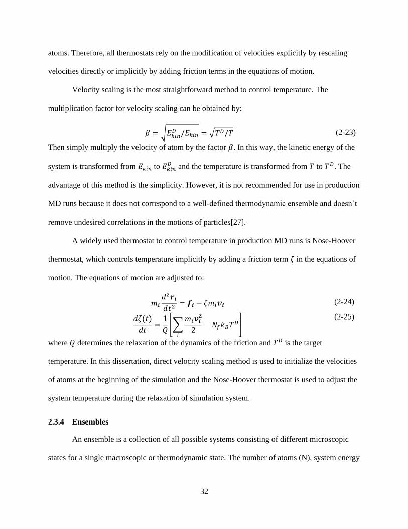
atoms. Therefore, all thermostats rely on the modification of velocities explicitly by rescaling

velocities directly or implicitly by adding friction terms in the equations of motion.

Velocity scaling is the most straightforward method to control temperature. The

multiplication factor for velocity scaling can be obtained by:

𝛽 = √𝐸𝑘𝑖𝑛𝐷 /𝐸𝑘𝑖𝑛 = √𝑇𝐷/𝑇 (2-23)

Then simply multiply the velocity of atom by the factor 𝛽. In this way, the kinetic energy of the

system is transformed from 𝐸𝑘𝑖𝑛 to 𝐸𝑘𝑖𝑛𝐷 and the temperature is transformed from 𝑇 to 𝑇𝐷. The

advantage of this method is the simplicity. However, it is not recommended for use in production

MD runs because it does not correspond to a well-defined thermodynamic ensemble and doesn’t

remove undesired correlations in the motions of particles[27].

A widely used thermostat to control temperature in production MD runs is Nose-Hoover

thermostat, which controls temperature implicitly by adding a friction term 휁 in the equations of

motion. The equations of motion are adjusted to:

𝑚𝑖

𝑑2𝒓𝑖

𝑑𝑡2= 𝒇𝒊 − 휁𝑚𝑖𝒗𝒊 (2-24)

𝑑휁(𝑡)

𝑑𝑡=

1

𝑄[∑

𝑚𝑖𝒗𝒊𝟐

2𝑖

− 𝑁𝑓𝑘𝐵𝑇𝐷] (2-25)

where 𝑄 determines the relaxation of the dynamics of the friction and 𝑇𝐷 is the target

temperature. In this dissertation, direct velocity scaling method is used to initialize the velocities

of atoms at the beginning of the simulation and the Nose-Hoover thermostat is used to adjust the

system temperature during the relaxation of simulation system.

2.3.4 Ensembles

An ensemble is a collection of all possible systems consisting of different microscopic

states for a single macroscopic or thermodynamic state. The number of atoms (N), system energy

33

(E), temperature (T), volume (V) and pressure (P) defines the thermodynamic state variables in

molecular dynamics. Various combinations of state variables can be controlled to produce

certain ensembles. The isobaric-isothermal ensemble (NPT), canonical ensemble (NVT) and

microcanonical ensemble (NVE) are common ensembles in MD. Since the temperature and

pressure is defined in the NPT ensemble, this ensemble is used to relax the system or achieve

specific temperature and pressure in the simulation. The volume and temperature are fixed in the

NVT ensemble. Therefore, it is used in the oxidation simulation of CF and char to prevent

dimensional changes of the simulation cell. In the NVE ensemble, the system energy is

conserved and there is no control of the temperature and pressure of the system.

34

CHAPTER 3

NANOINDENTATION OF ZRH2 BY MOLECULAR DYNAMICS SIMULATION*

2.4 Background

Pressurized water reactors (PWRs) and boiling water reactors (BWRs) are widely used as

commercial nuclear reactors around the world[28]. Because of their low thermal neutron

absorption, high corrosion resistance and excellent mechanical properties, zirconium-based

alloys such as Zircaloy[29] and ZIRLO[30] are used as fuel cladding to establish the first barrier

in preventing fission products from entering into the primary cooling circuit[31,32]. However,

excessive hydrogen generated in the reaction between water and zirconium precipitates as

zirconium hydride in the cladding; this can lead to reduction of the fracture toughness and

ductility of the clad, ultimately resulting in mechanical failure [33]. Therefore, understanding the

deformation behavior of zirconium hydrides will be helpful in improving the design and the

performance of the cladding. Many density functional theory (DFT) calculations have been

conducted to investigate the ground state properties of the Zr-H system, including the lattice

parameter, elastic constants, surface energy, and vacancy and interstitial formation energies [34–

36]. Although previous Molecular Dynamics (MD) simulations have focused on the investigation

of the hydrogen diffusion in Zr[37], deformation processes in the polycrystalline Zr[38],

nanoindentation of the Zr[39] and ZrO2/Zr[40], there has been little simulation work on the

deformation process in ZrHx.

Nanoindentation has been widely used in experiments to characterize the Young’s

modulus, yield stress, fracture toughness and deformation process of zirconium hydride at the

* The work described in this chapter has been published in L. Shi, M. L. Fullarton, and S. R. Phillpot.

"Nanoindentation of ZrH2 by molecular dynamics simulation." Journal of Nuclear Materials 540 (2020): 152391.

doi: 10.1016/j.jnucmat.2020.152391.

35

microscale[41–43]. However, it is still very challenging to observe the nucleation and

propagation of dislocations at the atomic scale. Nanoindentation by MD simulation has been

widely used to characterize the deformation processes at the atomic scale. For example, Li et al.

used nanoindentation simulation to identify the defect nucleation process resulting in hardening

in gold and gold alloys[44]. Fu et al. performed nanoindentation simulation on VN(001) films,

from which they identified the formation mechanism of dislocation loops and the initial plastic

deformation during the indentation[45]. Sun et al. used nanoindentation simulation to explore the

formation mechanism of the prismatic loops in the 3C-SiC single crystal[46]. Wang et al.

investigated the “double cross” splitting mechanism of single-crystal diamond using

nanoindentation simulation[47]. In this work we perform MD simulations of nanoindentation on

𝛿-ZrH2 with a spherical indenter to characterize the formation mechanism of dislocations at the

atomic level. In section 2.5, the methods employed in the work, the simulation setup, the

structure, and the slip system of ZrH2 are introduced. In Section 2.6, the influence of the indenter

speed and the influence of the thickness of the active layer during the nanoindentation are

analyzed. In Section 2.7, the effects of indentation on the <100> and <110> surface orientations

are discussed. The conclusions are in Section 2.8

2.5 Methods and Simulation Setup

2.5.1 Interatomic Potential

There are MEAM[37], EAM/ALLOY[48] and COMB3[49,50] interatomic potentials for

the Zr-H binary system. The MEAM and EAM/ALLOY potentials were specifically fitted for the

simulation of diffusion of hydrogen atoms in hcp 𝛼-Zr. As a result, they cannot be expected to

give a good description of the hydride. Indeed, both the MEAM and EAM/ALLOY potentials

predict the ZrHx structure to be mechanically unstable, which is contradicted by experiment. By

contrast, the COMB3 potential was fitted for Zr-H binary compounds and predicts a stable -

36

ZrH2 structure at 0 K and room temperature. Zhang et al. showed that the COMB3 potential is

capable of describing the homogenous hydride formation path in 𝛼-Zr and predicts a formation

energy for -ZrH1.0-2.0 which in good agreement with DFT results[51]. The stacking fault energy

(SFE) of α-Zr and the ζ hydride were also investigated by Zhang et al. For α-Zr, the stable and

unstable SFE were found to be 104 and 134mJ/m2 with the COMB potential. The same

properties calculated by DFT calculations[52] were 227 and 285 mJ/m2 respectively. For ζ-

hydride, a negative stable SFE was predicted by both the COMB potential (-51mJ/ m2) and DFT

calculations (-95mJ/ m2). Although the COMB potential underestimates the absolute values of

SFEs compared with DFT calculations, the shape of SFE curve is similar with that from previous

DFT calculations. We thus expect that the dislocation-related plastic processes predicted by

COMB will be consistent with those that would be obtained from ab initio DFT if such

simulations were possible on such large systems. While ZrH1.5-1.7 is most often observed as the

cubic ẟ-phase, the ground state of stoichiometric ZrH2 is actually the ε-phase, a tetragonally (c/a

=0.878) distorted fluorite structure. It was found that COMB3 could not describe both the -ZrH2

and -ZrH2 simultaneously; it was therefore parameterized to the -phase only, with the intent

that -phase compositions be approximated as the -phase. Therefore, in this work the

nanoindentation simulations on the stoichiometric composition use the cubic structure ẟ-ZrH2.

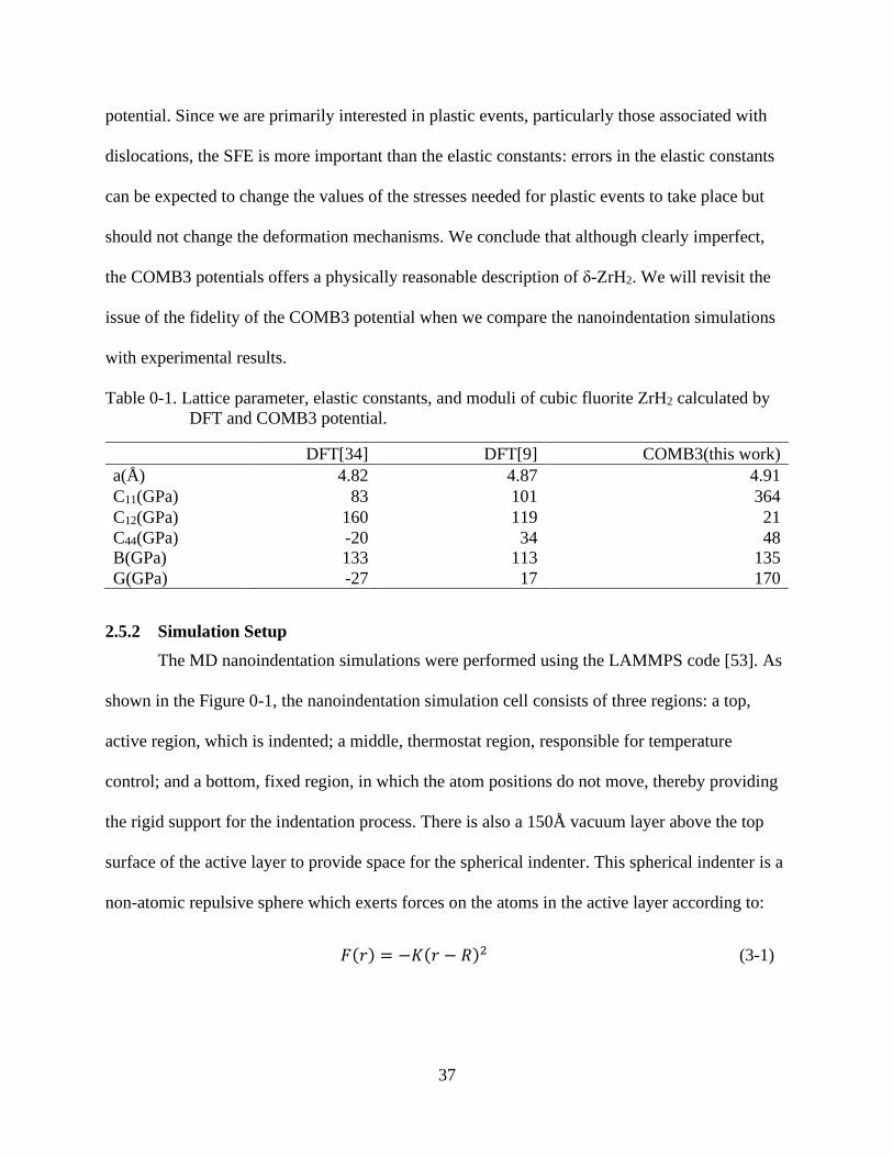
Table 0-1 lists the lattice parameter and elastic moduli of ẟ-ZrH2 calculated by COMB3

potential. The lattice parameter and bulk modulus, B, agree well with DFT values. However, the

individual elastic constants contributing to B = (1/3) (C11 + 2C12) do not agree well with the DFT

values. DFT calculations yield low, or in one case negative, values for C44 and the shear

constant, G=1/2(C11-C12), indicating the zero-temperature instability of stoichiometric -ZrH2.

Mechanical stability is ensured in MD simulations of δ-ZrH2 by the parameterization of COMB3

37

potential. Since we are primarily interested in plastic events, particularly those associated with

dislocations, the SFE is more important than the elastic constants: errors in the elastic constants

can be expected to change the values of the stresses needed for plastic events to take place but

should not change the deformation mechanisms. We conclude that although clearly imperfect,

the COMB3 potentials offers a physically reasonable description of ẟ-ZrH2. We will revisit the

issue of the fidelity of the COMB3 potential when we compare the nanoindentation simulations

with experimental results.

Table 0-1. Lattice parameter, elastic constants, and moduli of cubic fluorite ZrH2 calculated by

DFT and COMB3 potential.

DFT[34] DFT[9] COMB3(this work)

a(Å) 4.82 4.87 4.91

C11(GPa) 83 101 364

C12(GPa) 160 119 21

C44(GPa) -20 34 48

B(GPa) 133 113 135

G(GPa) -27 17 170

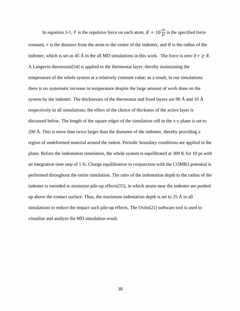
2.5.2 Simulation Setup

The MD nanoindentation simulations were performed using the LAMMPS code [53]. As

shown in the Figure 0-1, the nanoindentation simulation cell consists of three regions: a top,

active region, which is indented; a middle, thermostat region, responsible for temperature

control; and a bottom, fixed region, in which the atom positions do not move, thereby providing

the rigid support for the indentation process. There is also a 150Å vacuum layer above the top

surface of the active layer to provide space for the spherical indenter. This spherical indenter is a

non-atomic repulsive sphere which exerts forces on the atoms in the active layer according to:

𝐹(𝑟) = −𝐾(𝑟 − 𝑅)2 (3-1)

38

In equation 3-1, 𝐹 is the repulsive force on each atom, 𝐾 = 10𝑒𝑉

Å3 is the specified force

constant, 𝑟 is the distance from the atom to the center of the indenter, and 𝑅 is the radius of the

indenter, which is set as 45 Å in the all MD simulations in this work. The force is zero if 𝑟 ≥ 𝑅.

A Langevin thermostat[54] is applied to the thermostat layer, thereby maintaining the

temperature of the whole system at a relatively constant value; as a result, in our simulations

there is no systematic increase in temperature despite the large amount of work done on the

system by the indenter. The thicknesses of the thermostat and fixed layers are 90 Å and 10 Å

respectively in all simulations; the effect of the choice of thickness of the active layer is

discussed below. The length of the square edges of the simulation cell in the x-y plane is set to

200 Å. This is more than twice larger than the diameter of the indenter, thereby providing a

region of undeformed material around the indent. Periodic boundary conditions are applied in the

plane. Before the indentation simulation, the whole system is equilibrated at 300 K for 10 ps with

an integration time step of 1 fs. Charge equilibration in conjunction with the COMB3 potential is

performed throughout the entire simulation. The ratio of the indentation depth to the radius of the

indenter is intended to minimize pile-up effects[55], in which atoms near the indenter are pushed

up above the contact surface. Thus, the maximum indentation depth is set to 25 Å in all

simulations to reduce the impact such pile-up effects. The Ovito[21] software tool is used to

visualize and analyze the MD simulation result.

39

Figure 0-1. Sketch of the simulation system. Active layer, thermostat layer and fixed layer are

colored as green, orange, and blue, respectively. Only Zr atoms are shown in this

figure.

There are three zirconium hydride ZrHx phases reported in past investigations in

zircalloy: the metastable 𝛾-phase (fct, c/a>1), the 𝛿-phase with face centered cubic(fcc) structure,

and the 휀-phase with face centered tetragonal structure (fct, c/a<1) [56]. The 𝛾, 𝛿 and 휀 phases

have similar crystal structures and decreasing c/a ratio with increasing hydrogen concentration.

DFT calculations show the energy difference between the fcc structured -ZrH2 and ε-ZrH2 to be

only +7meV/atom[35] and thus fct ε-ZrH2 is more stable. For ε-ZrH2, c/a = 0.878[52], whereas

for -ZrH2 c/a = 1. Although this fcc structure is predicted by DFT calculation unstable due to

the negative G and C44 values in Table 0-1, the mechanical stability is ensured by the COMB3

potential by meeting the following stability conditions for cubic systems:

40

𝐶11 > 0, 𝐶44 > 0, 𝐶11 > |𝐶12|, (𝐶11 + 2𝐶12) > 0 (3-2)

The energy difference between fct ε-ZrH2 and δ-ZrH2 is +13meV/atom for the COMB

potential and is -7meV/atom in DFT calculations; as a result, the fct ε-ZrH2 transforms to fcc 𝛿-

ZrH2 after energy minimization using the COMB potential. We note that kT at room temperature

is 25 meV/atom; thus, all of these energy differences are very small. For this reason, and because

-ZrH2 is the most widely observed phase in fuel cladding, the fluorite fcc structure, -ZrH2, is

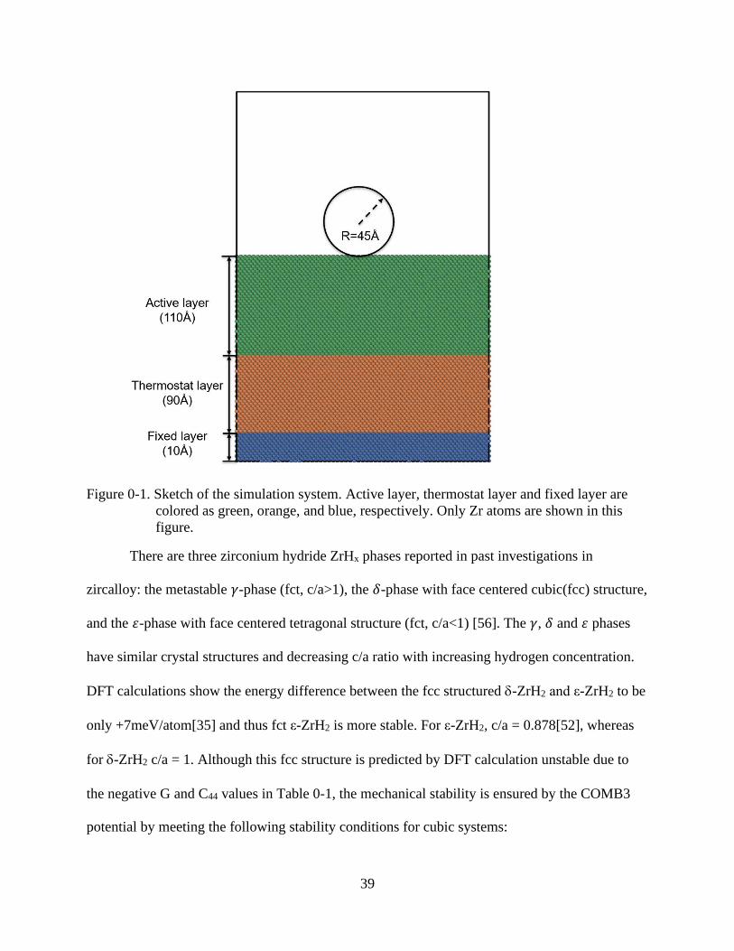
used in the simulation in place of ε-ZrH2. The [100] and [110] orientations are chosen in our

simulations to investigate the anisotropy of δ-ZrH2. For convenience in the simulation, a body

centered tetragonal unit cell, shown in Figure 0-2 A., is used, oriented along the [110], [110] and

[100] lattice directions. The relationship between the conventional cubic unit cell and the body

centered tetragonal unit cell is illustrated by a supercell of 𝛿-ZrH2 in Figure 0-2 B. This bct unit

cell contains both (100) and (110) planes. Indentation at different orientations is achieved by

choosing different planes of this bct unit cell. Nanoindentation on the (100) and (110) planes will

be studied in this work.

-ZrH2 has a fluorite-like structure where Zr atoms occupy the Bravais lattice sites of fcc

cubic sublattice and H occupies all the tetrahedral interstitial sites. Experiments on fluorite

structured CaF2[57] show that it has a {100}<011> primary slip system. There are three

orthogonal {100} plane in the fluorite structure. Each plane has two orthogonal <110> slip

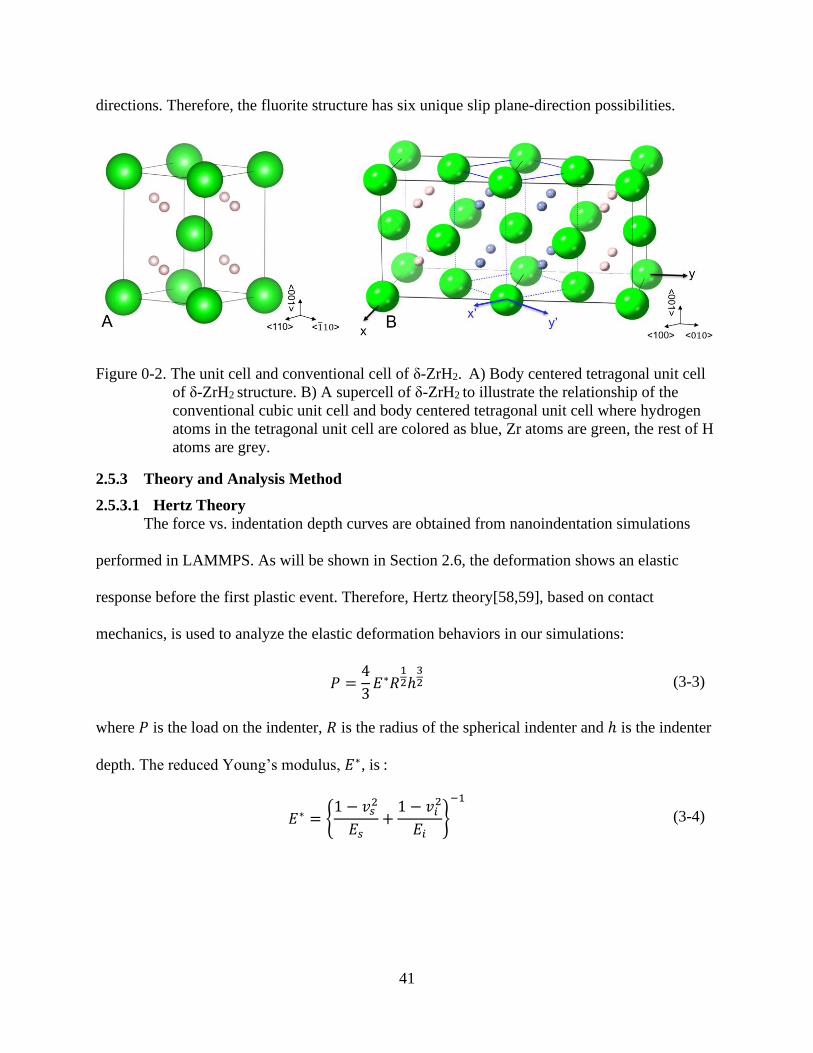
41

directions. Therefore, the fluorite structure has six unique slip plane-direction possibilities.

Figure 0-2. The unit cell and conventional cell of ẟ-ZrH2. A) Body centered tetragonal unit cell

of ẟ-ZrH2 structure. B) A supercell of ẟ-ZrH2 to illustrate the relationship of the

conventional cubic unit cell and body centered tetragonal unit cell where hydrogen

atoms in the tetragonal unit cell are colored as blue, Zr atoms are green, the rest of H

atoms are grey.

2.5.3 Theory and Analysis Method

2.5.3.1 Hertz Theory

The force vs. indentation depth curves are obtained from nanoindentation simulations

performed in LAMMPS. As will be shown in Section 2.6, the deformation shows an elastic

response before the first plastic event. Therefore, Hertz theory[58,59], based on contact

mechanics, is used to analyze the elastic deformation behaviors in our simulations:

𝑃 =4

3𝐸∗𝑅

12ℎ

32 (3-3)

where 𝑃 is the load on the indenter, 𝑅 is the radius of the spherical indenter and ℎ is the indenter

depth. The reduced Young’s modulus, 𝐸∗, is :

𝐸∗ = {1 − 𝑣𝑠

2

𝐸𝑠+

1 − 𝑣𝑖2

𝐸𝑖}

−1

(3-4)

42

where 𝐸𝑠 and s and 𝐸𝑖 and 𝑣𝑖 are Young’s moduli and Poisson ratios of the sample and

indenter, respectively. In this work, the force-field indenter is treated as an ideal hard indenter

with 𝐸𝑖 = ∞ and 𝑣𝑖 = 0. Thus 𝐸∗ =𝐸𝑠

1−𝑣𝑠2.

The hardness, 𝐻, can also be extracted from nanoindentation simulations and compared

with the prediction of Hertz Law:

𝐻 =𝑃

𝐴 (3-5)

where 𝐴 is the contact area between the indenter and the surface of the sample. The contact area

𝐴 is given by

𝐴 = 𝜋ℎ(2𝑅 − ℎ) (3-6)

where ℎ is the indentation depth and 𝑅 is the radius of the spherical indenter. In this work, we

calculate Young’s modulus and Poisson’s ratio for the (100) and (110) surfaces independently by

Hertz Law. The values of Young’s modulus, Poisson’s ratio, and reduced Young’s modulus

computed by the elastic constants are shown in Table 0-2 and are used in contact mechanics

calculations for the (100) and (110) surfaces. For isotropic materials, the Poisson’s ratio should

be within the bounds -1 to 0.5. However, because of the anisotropy of ZrH2, the Poisson’s ratio is

different in various directions, and can be negative or larger than 0.5 at the specific direction. It

is worth noting that the Poisson’s ratio on the (110) surface is larger than 0.5, which is measured

at the measurement direction [011] and stretched direction [011]. Cubic materials can have

positive values larger than 0.5 along diagonal direction of the face of the conventional cubic unit

cell; examples include RbBr (0.64), KI (0.61) and ReO3 (0.59); or negative values such as Li (-

0.52), CuAlNi (-0.65). [60–63]. Therefore, it is not unphysical that ZrH2 has a Poisson’s ratio

larger than 0.5 at direction [011]. For comparison, the Poisson’s ratio 𝑣0 in the [100] direction

43

was determined in a previous DFT calculation[34] to be 0.397, whereas COMB yields 0.055.

The difference between COMB and DFT results of Poisson’s ratios is a direct result of the

overestimation of C11 and underestimation of C12, which will be discussed in the Section 2.6.2.

The relationship between loads from two different indentation scenarios with different indenter

radii and depth for the same material can be expressed as

𝑃1

𝑃2= √

𝑅1

𝑅2(

ℎ1

ℎ2)

32 (3-7)

where 𝑃1 and 𝑃2 are the loads, ℎ1 and ℎ2 are indentation depths. To connect the simulations to

experiment, the experimental results, which are on 𝜇𝑁 scale, will be scaled to the 𝑛𝑁-scale

simulations according to equation 3-7.

Table 0-2. Young’s modulus, Poisson’s ratio, and reduced Young’s modulus of δ-ZrH2 in the

[100] and [110] orientations obtained from the COMB3 potential.

Orientation 𝐸𝑠(Gpa) 𝑣𝑠 𝐸∗(Gpa)

[100] 361 0.055 362

[110] 167 0.592 257

2.5.3.2 Local atomic symmetry analysis

The Central Symmetry Parameter (CSP)[64], widely used to characterize the symmetry

breaking in an atom’s local environment, can indicate the degree of disorder in the region of the

deformation, especially for bcc and fcc structures. Therefore, we characterize the local degree of

disorder during indentation by the CSP value. Because Zr atoms are located on the fcc sublattice

in 𝛿-ZrH2, the CSP value is also useful to characterize the local disorder of Zr atoms in this

work. The CSP for any given atom is defined by

𝐶𝑆𝑃 = ∑ |𝑹𝒊 + 𝑹𝒊+

𝑵𝟐

|2

𝑁2

𝑖=1

(3-8)

44

where 𝑁 is the number of the nearest neighbors of one atom, 𝑹𝒊 and 𝑹𝒊+

𝑵

𝟐

are the vectors from

the central atom to a pair of nearest neighbor atoms which has the smallest value of |𝑹𝒊 + 𝑹𝒊+

𝑵

𝟐

|.

As a result, The CSP is zero for an atom located on a lattice site in a perfect symmetric crystal

structure such as bcc or fcc. If there is a vacancy or an interstitial atom in the lattice, then the

CSP value of the atoms in the vicinity of the defect will be not zero. Also, the CSP value of the

atoms located in an inhomogeneously distorted lattice will be non-zero. Therefore, the CSP value

represents the degree of symmetry breaking in the lattice. Because the fcc structure has 12

nearest atoms, the value of 𝑁 is set to 12.

2.6 Analysis of Loading and Unloading

Nanoindentation is a well-established technique to investigate the time-dependent

deformation behavior and mechanical properties of materials. Nanoindentation by MD

simulation makes it possible to characterize the nucleation and growth of dislocations at an

atomic scale. During the loading process, the force applied on the indenter gradually increases as

the indenter moves deeper into the sample. The load vs. displacement curve should match the

solution of elastic contact mechanics developed by Hertz[65] before any sudden drop in the load

curve. The point where the sudden load drop occurs is often referred as the yield point in the

nanoindentation; One phenomenon that is sometimes observed in experiments is a sudden

displacement burst of the indenter, represented as a plateau in the load vs. displacement curve;

this is often referred to as pop-in behavior. If the force follows a 3/2 power rule with indenter

depth before the yield point, according to the equation 3-3 the loading is considered as elastic.

The load and unload force vs. depth curve will be identical in the elastic region. Both

experiments[66–68] and MD simulations[45,46,69] observed the nucleation of the dislocations at

the yield point, which associates the elastic-plastic transition with pop-in. However,

45

nanoindentation experiments on aluminum [70] also show that it is possible for there to be some

plasticity or nucleation of the dislocation before the pop-in during indentation, i.e., while the

material still displays elastic-like behavior. The indentation simulation could also be affected by

factors such as the speed of the indenter and the size of the thin film. Therefore, we will discuss

the influences of these factors, Hertz law and hardness in this section. The relations between

yield point and dislocations will be discussed in section 2.7.

2.6.1 The Effect of Indenter Speed and Active Layer Thickness

The system dimensions in these MD simulations are of the order of 100Å. We anticipate

that the indentation simulation result may be influenced by factors such as the thickness of the

active layers and the speed of the indenter. In order to investigate the influence of these factors,

we varied both the velocity of indenter and the thickness of the layers. Although the loading rates

of 25-50 ms-1 in the simulations are much faster than experiments, which ranges from nm s-1 to 1

mm s-1 [71], they are similar to the indentation rates in other MD simulations. [40,44,45,72].

Although this indentation speed is high, all of the processes seen in the simulation are at speeds

below the sound speed 2517 ms-1[36] and are thus, to a large extent, capturing the same physics

as would be captured by very slow speed simulations. It can be clearly seen in Figure 0-3 A. that

the load-displacement curves are essentially the same at the two speeds. Therefore, to improve

the simulation efficiency, 50 ms-1 is selected as the velocity of the indenter for the following

simulations.

To investigate the influence of the thickness of the active layer, we simulated several

nanoindentations with thicknesses of the active layer ranging from 30Å to 130Å on both the

(100) and (110) planes. Figure 0-3 B. and C. shows that the thickness of the active layer affects

the load vs. displacement curve. It can be clearly seen in Figure 0-3 B. that with an increase of

46

the thickness of the active layer, the load is slightly lower, especially for small thicknesses.

When the active layer thickness is small, the so-called substrate effect[73] is obvious. The

influence due to stiffness of the presence of the fixed layer cannot be neglected. When the total

thickness is larger, the substrate effect is weaker. Therefore, the influence of the thickness of the

different active layers can be ascribed to substrate effects. For the indentation on the (100) plane

this thickness is ~90 Å; for the indentation on the (110) plane it is a little larger, ~110 Å. For all

thicknesses, however, the indentation curves have the same general shape. Figure 0-3 B. shows

that the force and indentation depth for the first plastic event on the (100) plane does increase

with increasing thickness; however, the difference between the 90 Å and 110 Å thicknesses is

small, indicating that the asymptotic regime has been reached. These change in the load-

displacement curve’s shape with active layer’s thickness is most likely caused by the rigidity of

the lower fixed layer. The deferred plastic event on thicker active layers indicates that the

simulation cell shows more elastic behavior than with smaller thickness active layers. For a

thicker active layer, the dislocations have more space to grow before interacting with the atoms

in the fixed layer. In addition, it seems that this rigid layer prevents their transmission and results

in a stress in the system that tends to impede further plasticity events. For indentation on the

(110) plane, because no noticeable force drop is found in the load-displacement curve, we don’t

find a similarly impeded plastic deformation (see Figure 0-3 C.). As for the dislocations

themselves, their structures appear to be independent of the thickness of the active layer.

Therefore, the nanoindentation simulations with thickness 110Å and 130Å are selected for

dislocation analysis in the following sections for the (100) and (110) planes, respectively. Similar

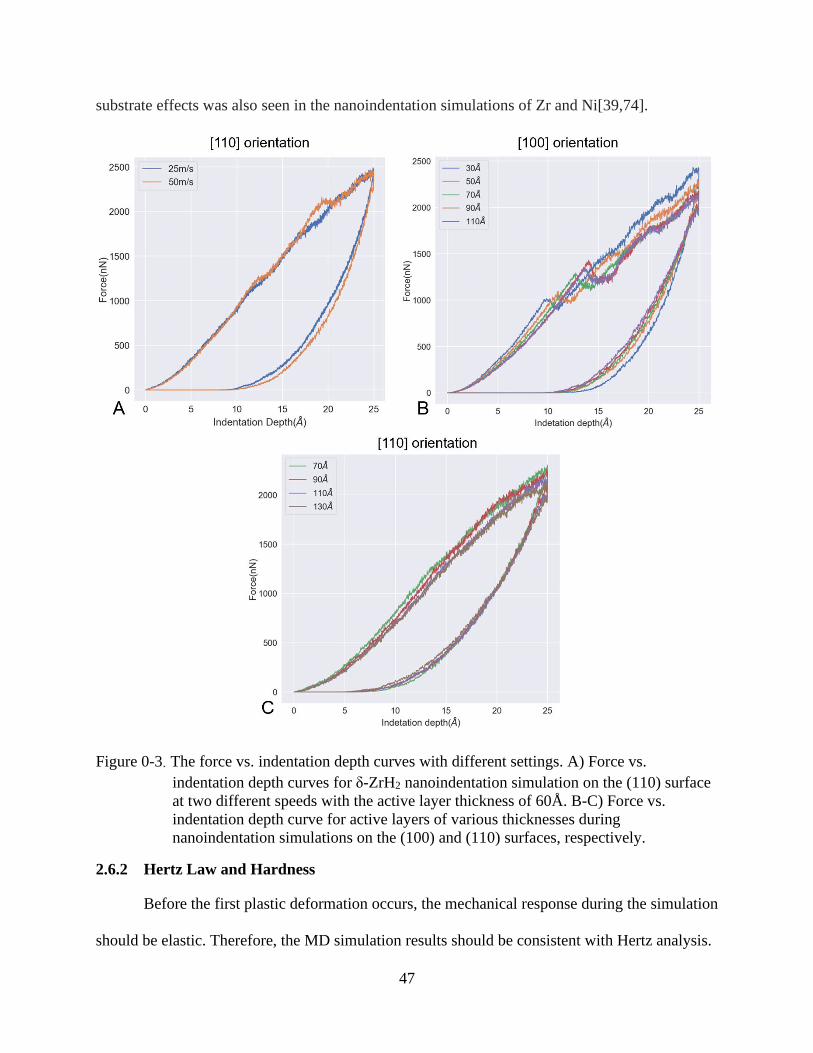
47

substrate effects was also seen in the nanoindentation simulations of Zr and Ni[39,74].

Figure 0-3. The force vs. indentation depth curves with different settings. A) Force vs.

indentation depth curves for δ-ZrH2 nanoindentation simulation on the (110) surface

at two different speeds with the active layer thickness of 60Å. B-C) Force vs.

indentation depth curve for active layers of various thicknesses during

nanoindentation simulations on the (100) and (110) surfaces, respectively.

2.6.2 Hertz Law and Hardness

Before the first plastic deformation occurs, the mechanical response during the simulation

should be elastic. Therefore, the MD simulation results should be consistent with Hertz analysis.

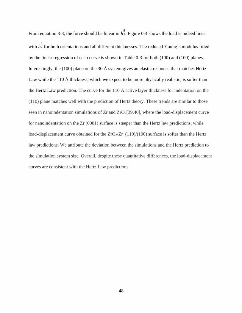
48

From equation 3-3, the force should be linear in ℎ3

2. Figure 0-4 shows the load is indeed linear

with ℎ3

2 for both orientations and all different thicknesses. The reduced Young’s modulus fitted

by the linear regression of each curve is shown in Table 0-3 for both (100) and (100) planes.

Interestingly, the (100) plane on the 30 Å system gives an elastic response that matches Hertz

Law while the 110 Å thickness, which we expect to be more physically realistic, is softer than

the Hertz Law prediction. The curve for the 110 Å active layer thickness for indentation on the

(110) plane matches well with the prediction of Hertz theory. These trends are similar to those

seen in nanoindentation simulations of Zr and ZrO2[39,40], where the load-displacement curve

for nanoindentation on the Zr (0001) surface is steeper than the Hertz law predictions, while

load-displacement curve obtained for the ZrO2/Zr (110)/(100) surface is softer than the Hertz

law predictions. We attribute the deviation between the simulations and the Hertz prediction to

the simulation system size. Overall, despite these quantitative differences, the load-displacement

curves are consistent with the Hertz Law predictions.

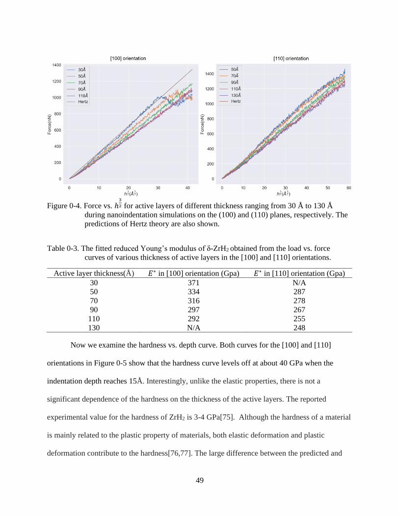
49

Figure 0-4. Force vs. ℎ3

2 for active layers of different thickness ranging from 30 Å to 130 Å

during nanoindentation simulations on the (100) and (110) planes, respectively. The

predictions of Hertz theory are also shown.

Table 0-3. The fitted reduced Young’s modulus of δ-ZrH2 obtained from the load vs. force

curves of various thickness of active layers in the [100] and [110] orientations.

Active layer thickness(Å) 𝐸∗ in [100] orientation (Gpa) 𝐸∗ in [110] orientation (Gpa)

30 371 N/A

50 334 287

70 316 278

90 297 267

110 292 255

130 N/A 248

Now we examine the hardness vs. depth curve. Both curves for the [100] and [110]

orientations in Figure 0-5 show that the hardness curve levels off at about 40 GPa when the

indentation depth reaches 15Å. Interestingly, unlike the elastic properties, there is not a

significant dependence of the hardness on the thickness of the active layers. The reported

experimental value for the hardness of ZrH2 is 3-4 GPa[75]. Although the hardness of a material

is mainly related to the plastic property of materials, both elastic deformation and plastic

deformation contribute to the hardness[76,77]. The large difference between the predicted and

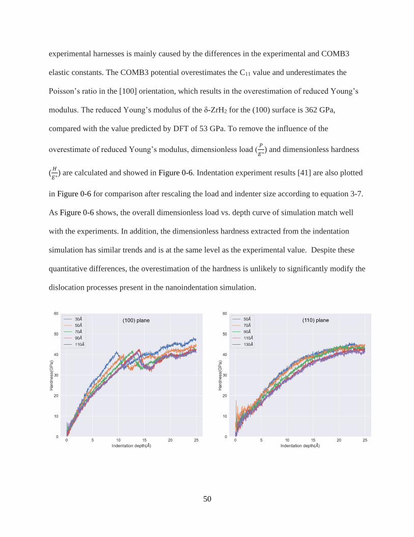
50

experimental harnesses is mainly caused by the differences in the experimental and COMB3

elastic constants. The COMB3 potential overestimates the C11 value and underestimates the

Poisson’s ratio in the [100] orientation, which results in the overestimation of reduced Young’s

modulus. The reduced Young’s modulus of the δ-ZrH2 for the (100) surface is 362 GPa,

compared with the value predicted by DFT of 53 GPa. To remove the influence of the

overestimate of reduced Young’s modulus, dimensionless load (𝑃

𝐸∗) and dimensionless hardness

(𝐻

𝐸∗) are calculated and showed in Figure 0-6. Indentation experiment results [41] are also plotted

in Figure 0-6 for comparison after rescaling the load and indenter size according to equation 3-7.

As Figure 0-6 shows, the overall dimensionless load vs. depth curve of simulation match well

with the experiments. In addition, the dimensionless hardness extracted from the indentation

simulation has similar trends and is at the same level as the experimental value. Despite these

quantitative differences, the overestimation of the hardness is unlikely to significantly modify the

dislocation processes present in the nanoindentation simulation.

51

Figure 0-5. Hardness vs. indentation depth with active layers of different thickness ranging from

30Å to 130Å during nanoindentation simulation on the (100) and (110) planes,

respectively.

Figure 0-6. A) Dimensionless load vs. indentation depth B) Dimensionless hardness vs.

indentation depth for (100) plane extracted from simulations and experiment.

2.7 Atomic-level Mechanisms

2.7.1 Nanoindentation on the (100) Surface

Figure 0-7 A. shows the load-displacement curve for the nanoindentation simulation on

the (100) δ-ZrH2 plane. The first load drop occurs at an indentation of 13.6 Å, which represents

the yield point. Figure 0-7 B. shows the sum of CSP values of the atoms vs. indentation depth of

nanoindentation on the (100) δ-ZrH2 plane. Figure 0-7 C.-F. show atomic-level processes that

take place during indentation. Only the Zr atoms are shown, colored by their CSP value, showing

only those with CSP values larger than 3, i.e., those in environments significantly different from

perfect fcc. We thus only see atoms at the surface (red atoms) and those atoms that are part of the

structure developed during the plastic deformation. As the depth of the indent increases, the

amount of disorder in the system increases and the total sum of the CSP values increases. The

CSP value begins to significantly increase after only 5Å of indentation, Figure 0-7 B. After the

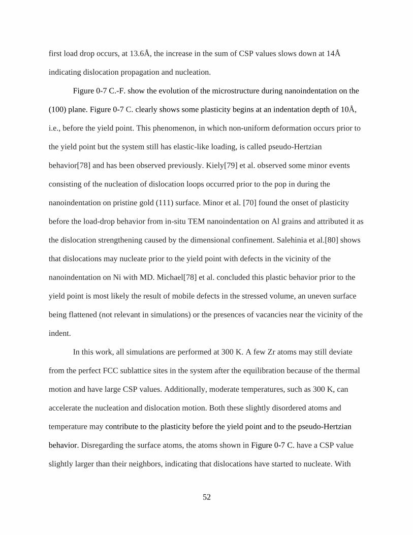
52

first load drop occurs, at 13.6Å, the increase in the sum of CSP values slows down at 14Å

indicating dislocation propagation and nucleation.

Figure 0-7 C.-F. show the evolution of the microstructure during nanoindentation on the

(100) plane. Figure 0-7 C. clearly shows some plasticity begins at an indentation depth of 10Å,

i.e., before the yield point. This phenomenon, in which non-uniform deformation occurs prior to

the yield point but the system still has elastic-like loading, is called pseudo-Hertzian

behavior[78] and has been observed previously. Kiely[79] et al. observed some minor events

consisting of the nucleation of dislocation loops occurred prior to the pop in during the

nanoindentation on pristine gold (111) surface. Minor et al. [70] found the onset of plasticity

before the load-drop behavior from in-situ TEM nanoindentation on Al grains and attributed it as

the dislocation strengthening caused by the dimensional confinement. Salehinia et al.[80] shows

that dislocations may nucleate prior to the yield point with defects in the vicinity of the

nanoindentation on Ni with MD. Michael[78] et al. concluded this plastic behavior prior to the

yield point is most likely the result of mobile defects in the stressed volume, an uneven surface

being flattened (not relevant in simulations) or the presences of vacancies near the vicinity of the

indent.

In this work, all simulations are performed at 300 K. A few Zr atoms may still deviate

from the perfect FCC sublattice sites in the system after the equilibration because of the thermal

motion and have large CSP values. Additionally, moderate temperatures, such as 300 K, can

accelerate the nucleation and dislocation motion. Both these slightly disordered atoms and

temperature may contribute to the plasticity before the yield point and to the pseudo-Hertzian

behavior. Disregarding the surface atoms, the atoms shown in Figure 0-7 C. have a CSP value

slightly larger than their neighbors, indicating that dislocations have started to nucleate. With

53

increased indentation depth, the dislocations gradually grow and move to the periodic edge of the

simulation cell. Figure 0-7 D.-F. show that four distinct dislocations grow along <110>

directions. Because the x-axis and y-axis both belong to <110> direction family, these

dislocations are symmetric in the x-y plane. Thus, all of these dislocations are of the {100}

<110> type.

To further investigate the pseudo-Hertzian behavior, nanoindentations on the (100) δ-

ZrH2 plane with indentation depths of 3Å, 6Å, 10Å and14Å were simulated. As shown in Figure

0-8 A., the load-displacement curve during the loading and unloading process for indentation

depth 3Å are almost identical indicating that no plasticity occurred during the simulation. For

indentation depth 6Å, which is slightly over the nucleation point of 5Å, the force on indenter

during unloading is slight smaller than during loading. When increasing the total indentation

depth, the difference of the force between loading and unloading increases and the enclosed area

of the load-displacement curve increases. Figure 0-8 B.-D. shows the final microstructure of the

δ-ZrH2 when the indenter finished the unloading process and was no longer in contact with the δ-

ZrH2 (100) surface. For the total indentation depth 3Å, Figure 0-9 B., no dislocation is found

after unloading, which indicates δ-ZrH2 has an elastic response during the whole nanoindentation

process. However, for the total indentation depths of 6Å and 10Å, obvious dislocations are

observed after unloading, as shown in the Figure 0-8 C. and D., which indicate the plasticity

occurs during the nanoindentation and is irreversible.

54

Figure 0-7. The indentation force vs. depth curves and simulation snapshots at different depth.

A) The load-displacement curve of the nanoindentation simulation on the (100) δ-

ZrH2 plane. B) The sum of CSP values of the atoms vs. indentation depth of

nanoindentation on the (100) δ-ZrH2 plane. (Only atoms of which CSP > 3 are

counted) C-F) The snapshots of microstructure evolution at different indentation

depth during nanoindentation simulation on the (100) δ-ZrH2 plane.

The load vs. depth curve for the [100] orientation in. Figure 0-7 A shows that the first

drop in load occurs at an indentation depth of 13.6Å. Originally, Zr atoms sit on an fcc sublattice

in the δ-ZrH2 and thus have 12 coordination neighbors. During nanoindentation there is a highly

deformed region, with 13-16 coordinated atoms, near the indenter, just beneath the surface at the

indentation depth of 13.6 Å, colored as red in Figure 0-9 A. and B. The xz-(100) and xz-(010)

sliced planes at the center of the indenter are presented in Figure 0-9 G.-I. The atoms indicated in

the circle at the xz-(010) plane in Figure 0-9 B. show that the atoms of the highly deformed

region move to a closed packed structure with ABAB stacking in the (010) direction. A similar

transformation was also observed in nanoindentation simulations of ZrO2 by Lu et al.[40]. In

55

contrast to the ZrO2 simulation, in which O atoms were shoved from the Zr atoms, the hydrogen

sublattice does not change during the indentation of δ-ZrH2 from depth 5 Å to 13.6 Å, except in

the highly deformed region, presumably because H atoms are very small in comparison to O

atoms, which are larger than Zr atoms. Figure 0-9 C. shows the H atoms still in a simple cubic

sublattice with only minor distortions at depth 13.6 Å. Thus, although the Zr sublattice is

distorted and transformed from fcc to ABAB stacking, the H atoms still have enough space to

remain in their original tetrahedral interstitial sites.

Figure 0-8. The snapshots of the final dislocations after unloading with different indentation

depth. A) The load-displacement curve of the nanoindentation simulation on the

(100) δ-ZrH2 plane with indentation depths of 3Å, 6Å, 10Å, 14Å and 25Å. B-D)

Snapshots of the final microstructure after unloading from indentation depths of 3Å,

6Å and 10 Å, respectively. (Only Zr atoms of which CSP > 3 are shown).

The empirical covalent radii of H and O are 37 pm and 73 pm, respectively. Based on the

lattice parameters of δ-ZrH2 and ZrO2, the ratio of the size of the H/O sitting in the tetrahedral

vacancy sites to the size of tetrahedron vacancy in ZrH2 and ZrO2 fcc lattice are 4.3% and 29.8%

respectively, calculated by the equation 4𝑟3

3𝑉𝑡𝑒𝑡𝑟𝑎, where 𝑟 is the radius of H/O atom and 𝑉𝑡𝑒𝑡𝑟𝑎 is

56

the size of the tetragonal site. In addition, because H atoms are small, the lattice parameter of δ-

ZrH2 is mainly determined by the size of the Zr atoms, while the lattice parameter of ZrO2 is

mainly determined by the size of oxygen atoms. As a result, oxygen atoms occupy a larger space

in the fcc lattice than the hydrogen atoms, accounting for the smaller distortion see in the H

sublattice comparted to the O sublattice during nanoindentation simulations.

The first load drop stops at an indentation depth of 14.3Å, Figure 0-7 A., at which the Zr

atoms in the highly deformed region become so disordered that they can no longer maintain

ABAB closed packing. Comparing Figure 0-9 D. with Figure 0-9 A., the highly deformed region

shrank from a rectangle to a triangle in the (100) plane. The atoms within the triangle in Figure

0-9 B. have lower coordination numbers and are more disordered. Comparing Figure 0-9 E. to

Figure 0-9 B., a different perspective of the same process as in panels A. and D., the atoms

within the indicated triangle in E. also become more disordered. The total number of atoms

within the highly deformed region decreases, which is manifested as an inflection point in the

total CSP value vs. indentation depth curve at depth 14.3 Å, as shown in Figure 0-7 B.

Comparison of Figure 0-9 C. with F. shows that at an indentation of 14.3 Å the H atoms also

cannot maintain a simple cubic lattice and become disordered.

57

Figure 0-9. Snapshots of the dislocations before and after the yielding point for the

nanoindentation on the (100) surface. A-B) (100) and (010) sliced planes of δ-ZrH2

at an indenter depth of 13.6Å during simulation for the [001] orientation C) Thin

slice of the H (100) plane in δ-ZrH2 at 13.6Å, where H atoms are colored yellow and

Zr atoms are hidden. D-E) (100) and (010) sliced planes of δ-ZrH2 at a depth of 14.3

Å during simulation for the [001] orientation F) Thin slice of the H (010) plane in δ-

ZrH2 at 14.3Å, where H atoms are colored yellow and Zr atoms are hidden. G-I) The

slice direction and which part we show for above figures. Atoms with CSP value < 3

and H atoms have been hidden in the (100) and (010) planes of δ-ZrH2.

Figure 0-10 shows snapshots of δ-ZrH2 at different indentation depths from three

orientations. As shown in Figure 0-10 A.-C., four {100} <110> dislocations grow obliquely

downwards beneath the xy-(001) surface. In addition, another dislocation grows under the lowest

point of the contact area due to the compressive force directly from the indenter. This plastic

deformation occurs in the highly deformed region, where all five dislocations start to nucleate,

causing the dramatic load drop at the indentation of 13.6Å. At an indentation depth of 14.3Å,

58

another four {100} <110> dislocations are nucleated, releasing the internal stress inside the bulk

ZrH2, making the load largely constant up to 16Å. These dislocations are indicated by the yellow

circles in Figure 0-10 E. and red arrows in Figure 0-10 F. These dislocations grow just beneath

and parallel to the surface of δ-ZrH2. In order to better illustrate these dislocations, the

propagation directions of these fully formed {100} <110> dislocations are indicated by red

arrows in Figure 0-11. The force continues to increase until 20Å, at which there is a small

plateau in the load; at this load small {100} <110> dislocations begin to nucleate as shown in the

yellow circles in Figure 0-10 I. and Figure 0-11, releasing some of the internal stress during

deformation. In conclusion, before the first load drop, four {100} <110> dislocations grow

obliquely under the surface. After the first load drop, another four {100} <110> dislocations

begin to grow just beneath and parallel to the surface of the bulk δ-ZrH2. There are also some

small dislocations nucleated, as shown in the yellow circle of Figure 0-11, which are not

reflected as a load drop or plateau in the load-displacement curve during the nanoindentation.

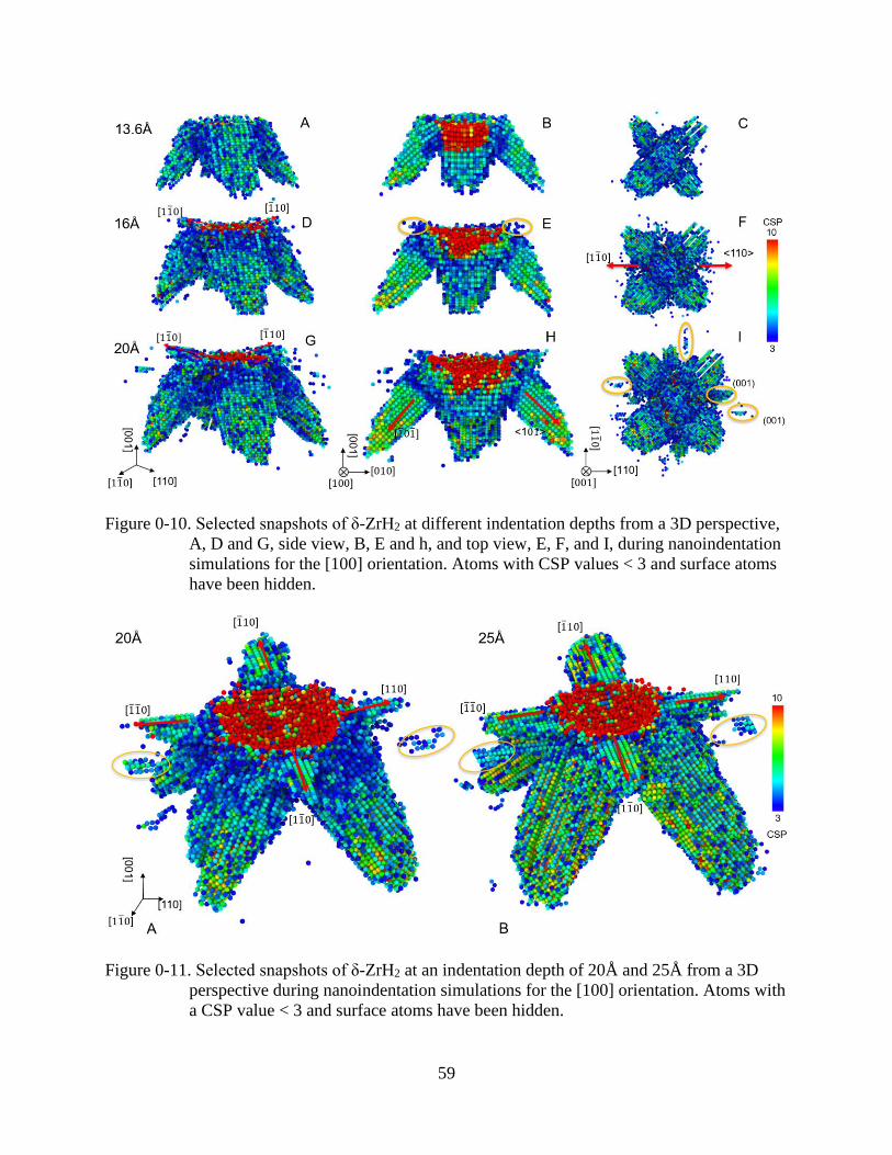
59

Figure 0-10. Selected snapshots of δ-ZrH2 at different indentation depths from a 3D perspective,

A, D and G, side view, B, E and h, and top view, E, F, and I, during nanoindentation

simulations for the [100] orientation. Atoms with CSP values < 3 and surface atoms

have been hidden.

Figure 0-11. Selected snapshots of δ-ZrH2 at an indentation depth of 20Å and 25Å from a 3D

perspective during nanoindentation simulations for the [100] orientation. Atoms with

a CSP value < 3 and surface atoms have been hidden.

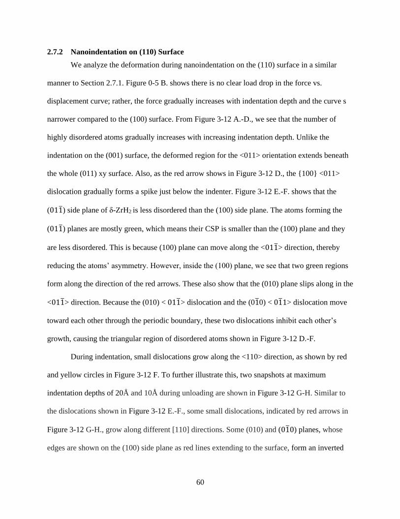
60

2.7.2 Nanoindentation on (110) Surface

We analyze the deformation during nanoindentation on the (110) surface in a similar

manner to Section 2.7.1. Figure 0-5 B. shows there is no clear load drop in the force vs.

displacement curve; rather, the force gradually increases with indentation depth and the curve s

narrower compared to the (100) surface. From Figure 3-12 A.-D., we see that the number of

highly disordered atoms gradually increases with increasing indentation depth. Unlike the

indentation on the (001) surface, the deformed region for the <011> orientation extends beneath

the whole (011) xy surface. Also, as the red arrow shows in Figure 3-12 D., the {100} <011>

dislocation gradually forms a spike just below the indenter. Figure 3-12 E.-F. shows that the

(011) side plane of δ-ZrH2 is less disordered than the (100) side plane. The atoms forming the

(011) planes are mostly green, which means their CSP is smaller than the (100) plane and they

are less disordered. This is because (100) plane can move along the <011> direction, thereby

reducing the atoms’ asymmetry. However, inside the (100) plane, we see that two green regions

form along the direction of the red arrows. These also show that the (010) plane slips along in the

<011> direction. Because the (010) < 011> dislocation and the (010) < 011> dislocation move

toward each other through the periodic boundary, these two dislocations inhibit each other’s

growth, causing the triangular region of disordered atoms shown in Figure 3-12 D.-F.

During indentation, small dislocations grow along the <110> direction, as shown by red

and yellow circles in Figure 3-12 F. To further illustrate this, two snapshots at maximum

indentation depths of 20Å and 10Å during unloading are shown in Figure 3-12 G-H. Similar to

the dislocations shown in Figure 3-12 E.-F., some small dislocations, indicated by red arrows in

Figure 3-12 G-H., grow along different [110] directions. Some (010) and (010) planes, whose

edges are shown on the (100) side plane as red lines extending to the surface, form an inverted

61

triangle shape. These planes slip from one side of the < 011> direction, overcoming the

resistance force dislocations on the (001) plane, cross the center of the (100) side plane and

become the red lines on the [100] plane. Thus, Figure 3-12 E.-H. show one (010) < 011> and

one (010) < 011> dislocation growing on the (100) side plane and moving towards each other.

Compared with Figure 3-12 E. and F., most of the disordered atoms in Figure 3-12 G. and H. are

colored green, indicating weak disorder. During the unloading process, some dislocations recede

and the degree of disorder at the upper corners on the (100) side plane reduces. However, the

maximum depth of the center spike-shaped dislocation remains the same during the process.

The cross-sectional views of the (110) and (100) planes are shown in Figure 0-13 A. and

B. It can be clearly seen in Figure 0-13 A. that there is a distinct M-shape hollow surrounding the

center spike dislocation. Because the atoms with a CSP value smaller than 3 are hidden, this

hollow represents atoms with very low disorder; i.e., they are close to being on symmetric lattice

sites. Atoms just beneath the indenter could either slip along the <011> direction parallel to the

page or along the <011> direction following the movement of the indenter. Therefore, several

different {100}[100] dislocations grow from these atoms, which significantly decreases the

amount of disorder and produces the hollow in Figure 0-13 A. and B. Another point of interest in

Figure 0-13 B. is that some Zr atoms, shown in the highly deformed region and marked by a

yellow circle, change structure to AAA closed packing, whereas atoms in the spike dislocation

region, marked by a red circle, remain in an fcc structure. As in the case of the [100] orientation,

most hydrogen atoms remain in the simple cubic sublattice with only a few H atoms very close

to the indenter becoming disordered.

62

Figure 0-12. The selected snapshots of δ-ZrH2 at different indentation depths from a 3D

perspective during nanoindentation simulations for the [110] orientation. Atoms

with a CSP value < 3 have been hidden.

63

Figure 0-13. Cross section of δ-ZrH2 at an indentation depth of 25Å during simulations for the

[110] orientation. Atoms with a CSP value < 3 have been hidden.

2.8 Summary

Molecular dynamics simulations of nanoindentation on the (100) and (110) planes of ẟ-

ZrH2 at 300 K are performed to investigate the deformation behavior and mechanisms using the

COMB3 potential. It is found that the indenter speed doesn’t have a significant influence on the

indentation results. When the thickness of the active layer is small, the substrate effect is clear.

The substrate effect becomes weaker with an increasing thickness of the active layer. The MD

simulation results agree well with Hertz Law predictions in elastic region. While the calculated

harnesses from the indentation of the (100) and (110) surfaces of δ-ZrH2 are higher than the

experimental values, the dimensionless load, (𝑃

𝐸∗), and hardness, (𝐻

𝐸∗), matches well with

experiment. Yield behaviors are observed on the (100) surface but not on the (110) surface. In

the highly deformed region, the Zr atom sublattice changes from an fcc structure to ABAB close

packing during nanoindentation until the first load drop, while the H atom sublattice remains a

64

simple cubic lattice due to the small atom size. The Zr and H atoms in the highly deformed

region become totally disordered after the load drop for nanoindentation on the (100) plane. We

find the dominant dislocation in the nanoindentation for both the (100) and (110) surfaces are

{100} <110> dislocations. The newly nucleated dislocations grow parallel with the surface after

yielding for indentation on the (100) surface with the increase of the depth. Small dislocations

are also observed to nucleate and grow along the <110> directions with the increase of the

indentation depth. In summary, we have clarified the deformation mechanism of δ-ZrH2 under

nanoindentation and described the factors that may influence the deformation, which not only

strengthens the understanding of how zirconium hydrides result in zircaloy cladding failure but

should also be helpful for developing the next generation of cladding.

65

CHAPTER 4

GENERATION AND CHARACTERIZATION OF AN IMPROVED CARBON FIBER

MODEL†

3.1 Background

Carbon fibers (CFs) have been developed for more than half a century because of their

low density, high elastic moduli, and good thermochemical stability[81]. One powerful property

of carbon fibers is that their thermo-physical and mechanical properties span a wide range and

can be easily modified for the desired applications[82,83]. Therefore, carbon fiber composites,

particularly those with polymeric matrices, have been widely used in, construction, automobile

parts, aircraft, space craft, and for sports equipment [84–86]. Carbon fiber composites such as the

phenolic-impregnated carbon ablator (PICA)[87], are uses in thermal protection systems in

spacecrafts due to their light weight and high temperature resistance.

The processing of CFs requires a series of steps, starting with the spinning of the

precursor, such as rayon, pitch or Polyacrylonitrile (PAN), followed by stabilization in air and

carbonization in an inert environment, both of which involve complex chemical reactions and

physical transformations[81]. The choice of the precursor and processing treatments controls the

microstructure of CFs, including crystallite size, alignment of crystallites, pore size distribution

and the degree of graphitization, which together largely determine the density, modulus, strength,

and thermal conductivity. For instance, improvement of the tensile modulus of PAN-based

carbon fiber can be achieved by increasing the alignment of the crystallites through increasing

the carbonization temperature, albeit at the expense of the tensile and compressive strength[88].

† The work described in this chapter has been published in L. Shi, M. Sessim, M. R. Tonks, and S. R. Phillpot.

"Generation and characterization of an improved carbon fiber model by molecular dynamics." Carbon 172, 232-244

(2021). doi: 10.1016/j.carbon.2020.11.011

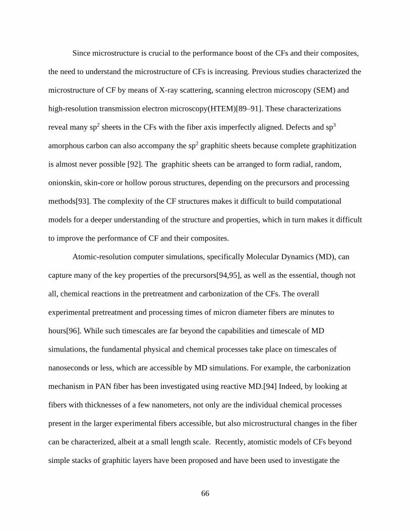
66

Since microstructure is crucial to the performance boost of the CFs and their composites,

the need to understand the microstructure of CFs is increasing. Previous studies characterized the

microstructure of CF by means of X-ray scattering, scanning electron microscopy (SEM) and

high-resolution transmission electron microscopy(HTEM)[89–91]. These characterizations

reveal many sp2 sheets in the CFs with the fiber axis imperfectly aligned. Defects and sp3

amorphous carbon can also accompany the sp2 graphitic sheets because complete graphitization

is almost never possible [92]. The graphitic sheets can be arranged to form radial, random,

onionskin, skin-core or hollow porous structures, depending on the precursors and processing

methods[93]. The complexity of the CF structures makes it difficult to build computational

models for a deeper understanding of the structure and properties, which in turn makes it difficult

to improve the performance of CF and their composites.

Atomic-resolution computer simulations, specifically Molecular Dynamics (MD), can

capture many of the key properties of the precursors[94,95], as well as the essential, though not

all, chemical reactions in the pretreatment and carbonization of the CFs. The overall

experimental pretreatment and processing times of micron diameter fibers are minutes to

hours[96]. While such timescales are far beyond the capabilities and timescale of MD

simulations, the fundamental physical and chemical processes take place on timescales of

nanoseconds or less, which are accessible by MD simulations. For example, the carbonization

mechanism in PAN fiber has been investigated using reactive MD.[94] Indeed, by looking at

fibers with thicknesses of a few nanometers, not only are the individual chemical processes

present in the larger experimental fibers accessible, but also microstructural changes in the fiber

can be characterized, albeit at a small length scale. Recently, atomistic models of CFs beyond

simple stacks of graphitic layers have been proposed and have been used to investigate the

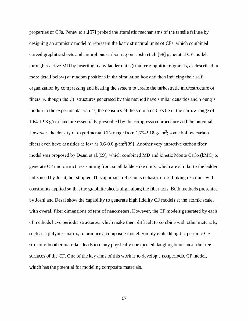
67

properties of CFs. Penev et al.[97] probed the atomistic mechanisms of the tensile failure by

designing an atomistic model to represent the basic structural units of CFs, which combined

curved graphitic sheets and amorphous carbon region. Joshi et al. [98] generated CF models

through reactive MD by inserting many ladder units (smaller graphitic fragments, as described in

more detail below) at random positions in the simulation box and then inducing their self-

organization by compressing and heating the system to create the turbostratic microstructure of

fibers. Although the CF structures generated by this method have similar densities and Young’s

moduli to the experimental values, the densities of the simulated CFs lie in the narrow range of

1.64-1.93 g/cm3 and are essentially prescribed by the compression procedure and the potential.

However, the density of experimental CFs range from 1.75-2.18 g/cm3; some hollow carbon

fibers even have densities as low as 0.6-0.8 g/cm3[89]. Another very attractive carbon fiber

model was proposed by Desai et al.[99], which combined MD and kinetic Monte Carlo (kMC) to

generate CF microstructures starting from small ladder-like units, which are similar to the ladder

units used by Joshi, but simpler. This approach relies on stochastic cross-linking reactions with

constraints applied so that the graphitic sheets align along the fiber axis. Both methods presented

by Joshi and Desai show the capability to generate high fidelity CF models at the atomic scale,

with overall fiber dimensions of tens of nanometers. However, the CF models generated by each

of methods have periodic structures, which make them difficult to combine with other materials,

such as a polymer matrix, to produce a composite model. Simply embedding the periodic CF

structure in other materials leads to many physically unexpected dangling bonds near the free

surfaces of the CF. One of the key aims of this work is to develop a nonperiodic CF model,

which has the potential for modeling composite materials.

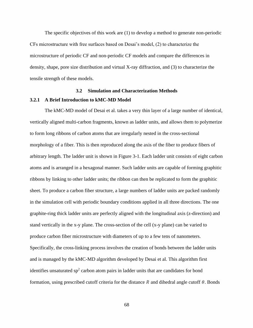
68

The specific objectives of this work are (1) to develop a method to generate non-periodic

CFs microstructure with free surfaces based on Desai’s model, (2) to characterize the

microstructure of periodic CF and non-periodic CF models and compare the differences in

density, shape, pore size distribution and virtual X-ray diffraction, and (3) to characterize the

tensile strength of these models.

3.2 Simulation and Characterization Methods

3.2.1 A Brief Introduction to kMC-MD Model

The kMC-MD model of Desai et al. takes a very thin layer of a large number of identical,

vertically aligned multi-carbon fragments, known as ladder units, and allows them to polymerize

to form long ribbons of carbon atoms that are irregularly nested in the cross-sectional

morphology of a fiber. This is then reproduced along the axis of the fiber to produce fibers of

arbitrary length. The ladder unit is shown in Figure 3-1. Each ladder unit consists of eight carbon

atoms and is arranged in a hexagonal manner. Such ladder units are capable of forming graphitic

ribbons by linking to other ladder units; the ribbon can then be replicated to form the graphitic

sheet. To produce a carbon fiber structure, a large numbers of ladder units are packed randomly

in the simulation cell with periodic boundary conditions applied in all three directions. The one

graphite-ring thick ladder units are perfectly aligned with the longitudinal axis (z-direction) and

stand vertically in the x-y plane. The cross-section of the cell (x-y plane) can be varied to

produce carbon fiber microstructure with diameters of up to a few tens of nanometers.

Specifically, the cross-linking process involves the creation of bonds between the ladder units

and is managed by the kMC-MD algorithm developed by Desai et al. This algorithm first

identifies unsaturated sp2 carbon atom pairs in ladder units that are candidates for bond

formation, using prescribed cutoff criteria for the distance 𝑅 and dihedral angle cutoff 휃. Bonds

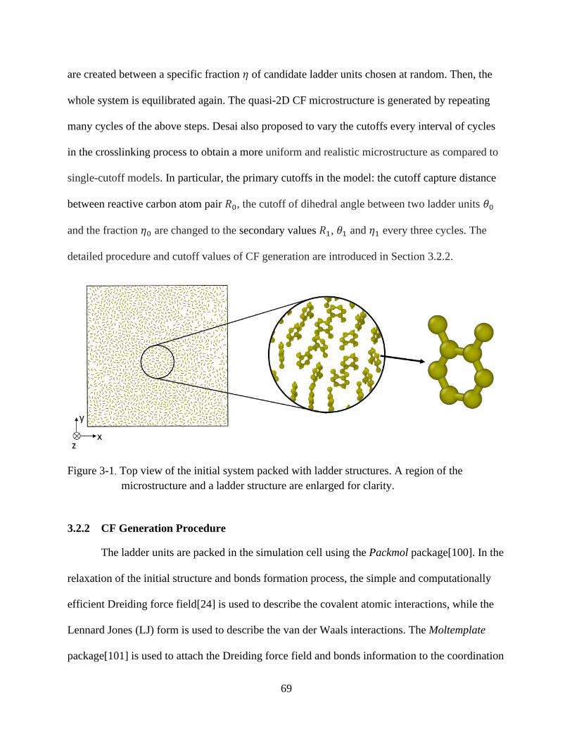
69

are created between a specific fraction 휂 of candidate ladder units chosen at random. Then, the

whole system is equilibrated again. The quasi-2D CF microstructure is generated by repeating

many cycles of the above steps. Desai also proposed to vary the cutoffs every interval of cycles

in the crosslinking process to obtain a more uniform and realistic microstructure as compared to

single-cutoff models. In particular, the primary cutoffs in the model: the cutoff capture distance

between reactive carbon atom pair 𝑅0, the cutoff of dihedral angle between two ladder units 휃0

and the fraction 휂0 are changed to the secondary values 𝑅1, 휃1 and 휂1 every three cycles. The

detailed procedure and cutoff values of CF generation are introduced in Section 3.2.2.

Figure 3-1. Top view of the initial system packed with ladder structures. A region of the

microstructure and a ladder structure are enlarged for clarity.

3.2.2 CF Generation Procedure

The ladder units are packed in the simulation cell using the Packmol package[100]. In the

relaxation of the initial structure and bonds formation process, the simple and computationally

efficient Dreiding force field[24] is used to describe the covalent atomic interactions, while the

Lennard Jones (LJ) form is used to describe the van der Waals interactions. The Moltemplate

package[101] is used to attach the Dreiding force field and bonds information to the coordination

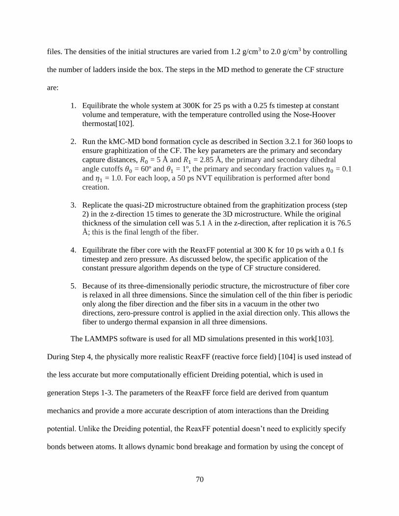
70

files. The densities of the initial structures are varied from 1.2 g/cm3 to 2.0 g/cm3 by controlling

the number of ladders inside the box. The steps in the MD method to generate the CF structure

are:

1. Equilibrate the whole system at 300K for 25 ps with a 0.25 fs timestep at constant

volume and temperature, with the temperature controlled using the Nose-Hoover

thermostat[102].

2. Run the kMC-MD bond formation cycle as described in Section 3.2.1 for 360 loops to

ensure graphitization of the CF. The key parameters are the primary and secondary

capture distances, 𝑅0 = 5 Å and 𝑅1 = 2.85 Å, the primary and secondary dihedral

angle cutoffs 휃0 = 60º and 휃1 = 1º, the primary and secondary fraction values 휂0 = 0.1

and 휂1 = 1.0. For each loop, a 50 ps NVT equilibration is performed after bond

creation.

3. Replicate the quasi-2D microstructure obtained from the graphitization process (step

2) in the z-direction 15 times to generate the 3D microstructure. While the original

thickness of the simulation cell was 5.1 Å in the z-direction, after replication it is 76.5

Å; this is the final length of the fiber.

4. Equilibrate the fiber core with the ReaxFF potential at 300 K for 10 ps with a 0.1 fs

timestep and zero pressure. As discussed below, the specific application of the

constant pressure algorithm depends on the type of CF structure considered.

5. Because of its three-dimensionally periodic structure, the microstructure of fiber core

is relaxed in all three dimensions. Since the simulation cell of the thin fiber is periodic

only along the fiber direction and the fiber sits in a vacuum in the other two

directions, zero-pressure control is applied in the axial direction only. This allows the

fiber to undergo thermal expansion in all three dimensions.

The LAMMPS software is used for all MD simulations presented in this work[103].

During Step 4, the physically more realistic ReaxFF (reactive force field) [104] is used instead of

the less accurate but more computationally efficient Dreiding potential, which is used in

generation Steps 1-3. The parameters of the ReaxFF force field are derived from quantum

mechanics and provide a more accurate description of atom interactions than the Dreiding

potential. Unlike the Dreiding potential, the ReaxFF potential doesn’t need to explicitly specify

bonds between atoms. It allows dynamic bond breakage and formation by using the concept of

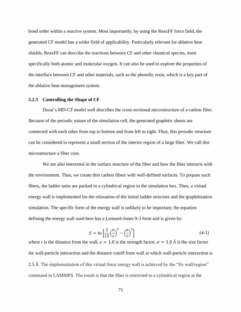
71

bond order within a reactive system. Most importantly, by using the ReaxFF force field, the

generated CF model has a wider field of applicability. Particularly relevant for ablative heat

shields, ReaxFF can describe the reactions between CF and other chemical species, most

specifically both atomic and molecular oxygen. It can also be used to explore the properties of

the interface between CF and other materials, such as the phenolic resin, which is a key part of

the ablative heat management system.

3.2.3 Controlling the Shape of CF

Desai’s MD-CF model well describes the cross-sectional microstructure of a carbon fiber.

Because of the periodic nature of the simulation cell, the generated graphitic sheets are

connected with each other from top to bottom and from left to right. Thus, this periodic structure

can be considered to represent a small section of the interior region of a large fiber. We call this

microstructure a fiber core.

We are also interested in the surface structure of the fiber and how the fiber interacts with

the environment. Thus, we create thin carbon fibers with well-defined surfaces. To prepare such

fibers, the ladder units are packed in a cylindrical region in the simulation box. Then, a virtual

energy wall is implemented for the relaxation of the initial ladder structure and the graphitization

simulation. The specific form of the energy wall is unlikely to be important; the equation

defining the energy wall used here has a Lennard-Jones 9-3 form and is given by:

𝐸 = 4𝜖 [2

15(

𝜎

𝑟)

9

− (𝜎

𝑟)

3

] (4-1)

where r is the distance from the wall, 𝜖 = 1.0 is the strength factor, 𝜎 = 1.0 Å is the size factor

for wall-particle interaction and the distance cutoff from wall at which wall-particle interaction is

2.5 Å. The implementation of this virtual force energy wall is achieved by the “fix wall/region”

command in LAMMPS. The result is that the fiber is restricted to a cylindrical region at the

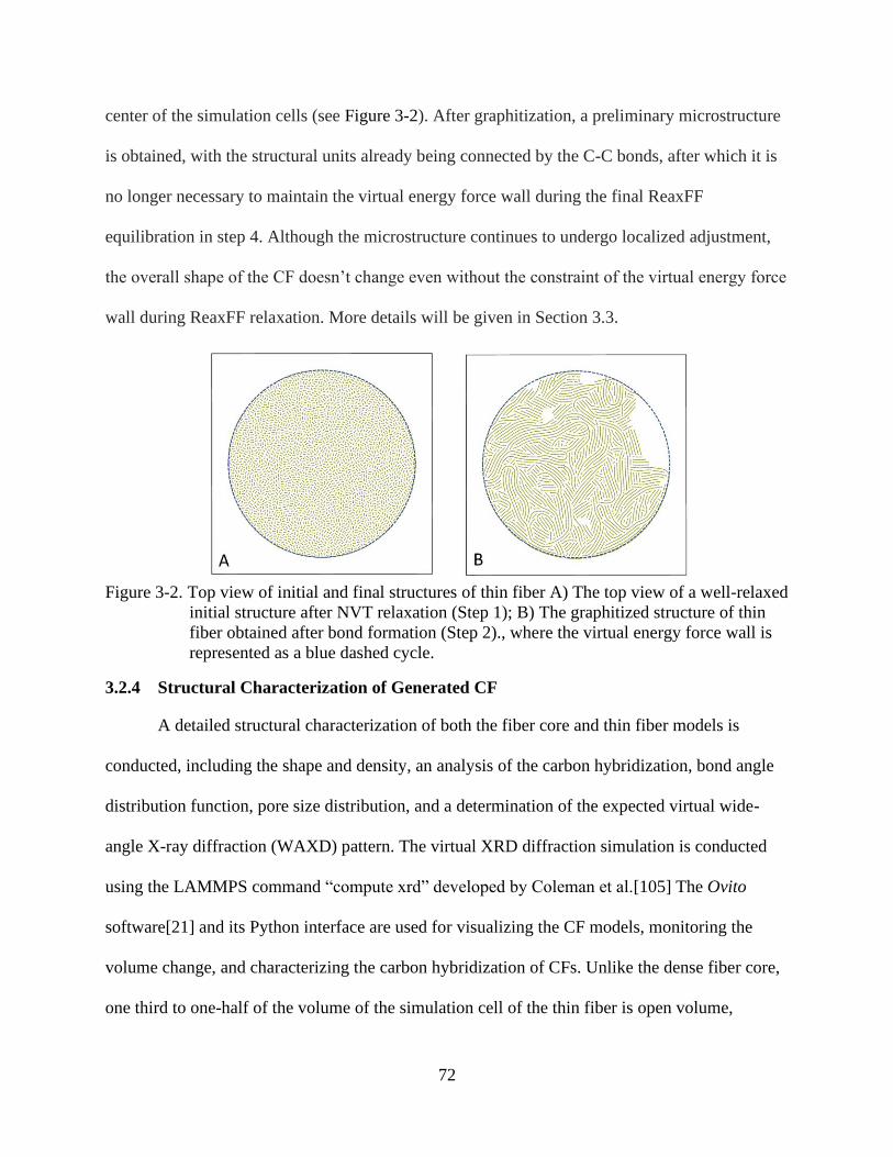
72

center of the simulation cells (see Figure 3-2). After graphitization, a preliminary microstructure

is obtained, with the structural units already being connected by the C-C bonds, after which it is

no longer necessary to maintain the virtual energy force wall during the final ReaxFF

equilibration in step 4. Although the microstructure continues to undergo localized adjustment,

the overall shape of the CF doesn’t change even without the constraint of the virtual energy force

wall during ReaxFF relaxation. More details will be given in Section 3.3.

Figure 3-2. Top view of initial and final structures of thin fiber A) The top view of a well-relaxed

initial structure after NVT relaxation (Step 1); B) The graphitized structure of thin

fiber obtained after bond formation (Step 2)., where the virtual energy force wall is

represented as a blue dashed cycle.

3.2.4 Structural Characterization of Generated CF

A detailed structural characterization of both the fiber core and thin fiber models is

conducted, including the shape and density, an analysis of the carbon hybridization, bond angle

distribution function, pore size distribution, and a determination of the expected virtual wide-

angle X-ray diffraction (WAXD) pattern. The virtual XRD diffraction simulation is conducted

using the LAMMPS command “compute xrd” developed by Coleman et al.[105] The Ovito

software[21] and its Python interface are used for visualizing the CF models, monitoring the

volume change, and characterizing the carbon hybridization of CFs. Unlike the dense fiber core,

one third to one-half of the volume of the simulation cell of the thin fiber is open volume,

73

external to the fiber surface. This enables the thin fiber to develop a three-dimensional irregular

shape during the ReaxFF equilibration in generation step 4. The surface irregularity makes the

calculation of the volume of the fiber more difficult; thus, to accurately compute the volume of

thin fiber, the “Construct Surface Mesh” modifier of Ovito is used to construct a polyhedral

surface mesh around the carbon atoms (see Figure 3-3); the actual volume of the fiber is then

determined from the enclosed area. To construct a surface mesh, a virtual probe sphere is used to

identify the accessible open region where the sphere does not touch any atom. In this work the

radius of the virtual probe sphere to identify the open area is chosen to be 12 Å; this avoids

counting small internal cavities or pores inside CF as open regions. A pore size distribution

(PSD) calculation code[106], suitable for the thin and fiber core model was developed, building

on the code of Joshi et al[107], in which the pore size is defined as the maximum distance

between two point within the pore. However, our code also filters out the open area outside the

thin fiber, thereby capturing the internal porosity. In addition, the efficiency is also improved by

replacing the for loops with graph networks[108] using the Boost graph library[109] during the

atom bins connectivity check.

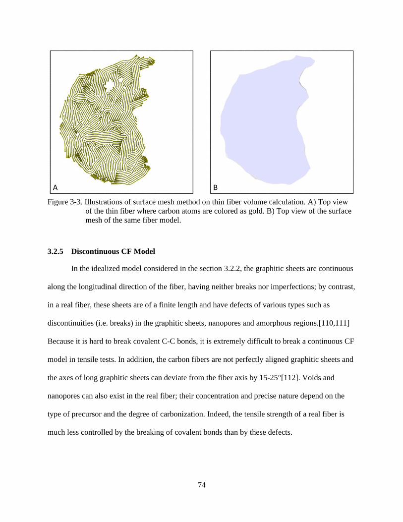
74

Figure 3-3. Illustrations of surface mesh method on thin fiber volume calculation. A) Top view

of the thin fiber where carbon atoms are colored as gold. B) Top view of the surface

mesh of the same fiber model.

3.2.5 Discontinuous CF Model

In the idealized model considered in the section 3.2.2, the graphitic sheets are continuous

along the longitudinal direction of the fiber, having neither breaks nor imperfections; by contrast,

in a real fiber, these sheets are of a finite length and have defects of various types such as

discontinuities (i.e. breaks) in the graphitic sheets, nanopores and amorphous regions.[110,111]

Because it is hard to break covalent C-C bonds, it is extremely difficult to break a continuous CF

model in tensile tests. In addition, the carbon fibers are not perfectly aligned graphitic sheets and

the axes of long graphitic sheets can deviate from the fiber axis by 15-25°[112]. Voids and

nanopores can also exist in the real fiber; their concentration and precise nature depend on the

type of precursor and the degree of carbonization. Indeed, the tensile strength of a real fiber is

much less controlled by the breaking of covalent bonds than by these defects.

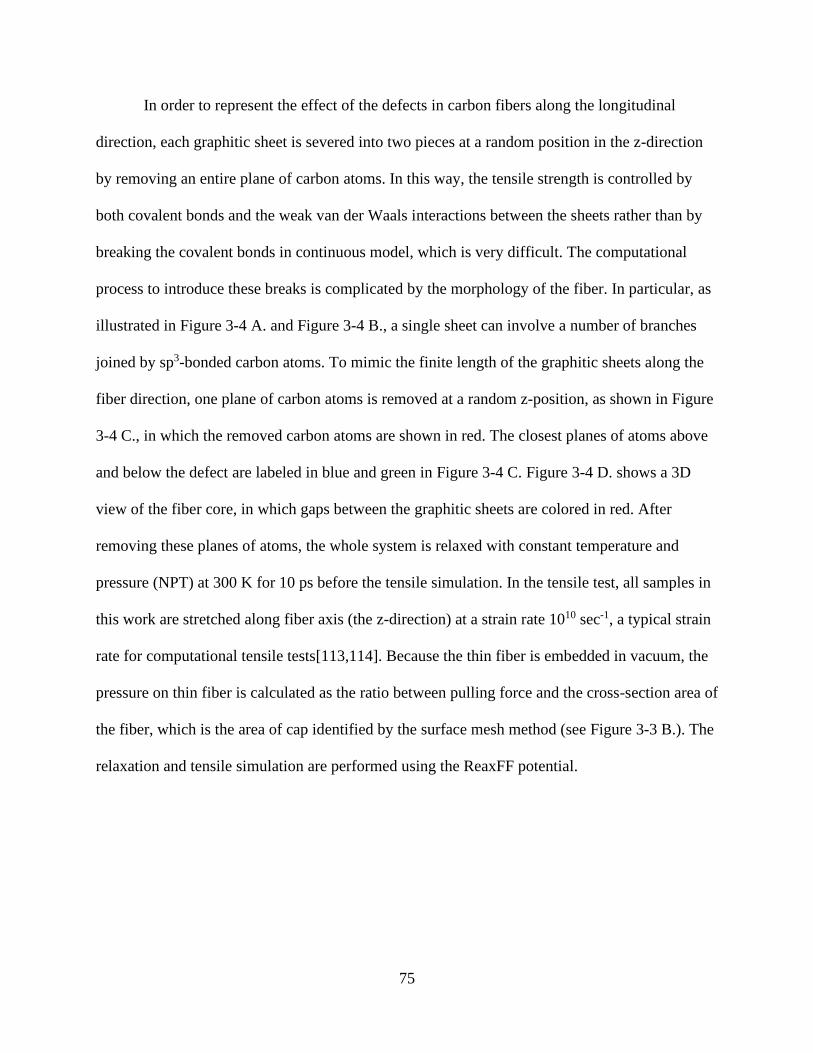
75

In order to represent the effect of the defects in carbon fibers along the longitudinal

direction, each graphitic sheet is severed into two pieces at a random position in the z-direction

by removing an entire plane of carbon atoms. In this way, the tensile strength is controlled by

both covalent bonds and the weak van der Waals interactions between the sheets rather than by

breaking the covalent bonds in continuous model, which is very difficult. The computational

process to introduce these breaks is complicated by the morphology of the fiber. In particular, as

illustrated in Figure 3-4 A. and Figure 3-4 B., a single sheet can involve a number of branches

joined by sp3-bonded carbon atoms. To mimic the finite length of the graphitic sheets along the

fiber direction, one plane of carbon atoms is removed at a random z-position, as shown in Figure

3-4 C., in which the removed carbon atoms are shown in red. The closest planes of atoms above

and below the defect are labeled in blue and green in Figure 3-4 C. Figure 3-4 D. shows a 3D

view of the fiber core, in which gaps between the graphitic sheets are colored in red. After

removing these planes of atoms, the whole system is relaxed with constant temperature and

pressure (NPT) at 300 K for 10 ps before the tensile simulation. In the tensile test, all samples in

this work are stretched along fiber axis (the z-direction) at a strain rate 1010 sec-1, a typical strain

rate for computational tensile tests[113,114]. Because the thin fiber is embedded in vacuum, the

pressure on thin fiber is calculated as the ratio between pulling force and the cross-section area of

the fiber, which is the area of cap identified by the surface mesh method (see Figure 3-3 B.). The

relaxation and tensile simulation are performed using the ReaxFF potential.

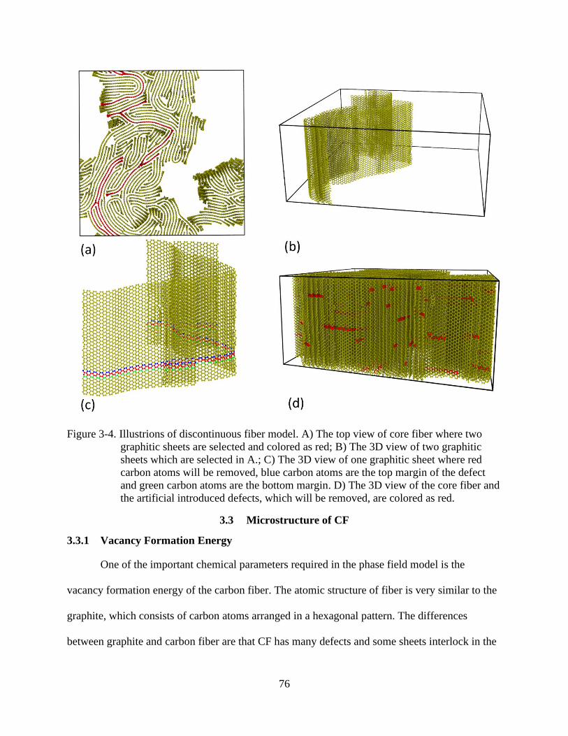
76

Figure 3-4. Illustrions of discontinuous fiber model. A) The top view of core fiber where two

graphitic sheets are selected and colored as red; B) The 3D view of two graphitic

sheets which are selected in A.; C) The 3D view of one graphitic sheet where red

carbon atoms will be removed, blue carbon atoms are the top margin of the defect

and green carbon atoms are the bottom margin. D) The 3D view of the core fiber and

the artificial introduced defects, which will be removed, are colored as red.

3.3 Microstructure of CF

3.3.1 Vacancy Formation Energy

One of the important chemical parameters required in the phase field model is the

vacancy formation energy of the carbon fiber. The atomic structure of fiber is very similar to the

graphite, which consists of carbon atoms arranged in a hexagonal pattern. The differences

between graphite and carbon fiber are that CF has many defects and some sheets interlock in the

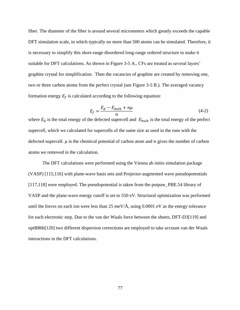
77

fiber. The diameter of the fiber is around several micrometers which greatly exceeds the capable

DFT simulation scale, in which typically no more than 500 atoms can be simulated. Therefore, it

is necessary to simplify this short-range disordered long-range ordered structure to make it

suitable for DFT calculations. As shown in Figure 3-5 A., CFs are treated as several layers’

graphite crystal for simplification. Then the vacancies of graphite are created by removing one,

two or three carbon atoms from the perfect crystal (see Figure 3-5 B.). The averaged vacancy

formation energy 𝐸𝑓 is calculated according to the following equation:

𝐸𝑓 =𝐸𝑑 − 𝐸𝑏𝑢𝑙𝑘 + 𝑛𝜇

𝑛 (4-2)

where 𝐸𝑑 is the total energy of the defected supercell and 𝐸𝑏𝑢𝑙𝑘 is the total energy of the perfect

supercell, which we calculated for supercells of the same size as used in the runs with the

defected supercell. 𝜇 is the chemical potential of carbon atom and 𝑛 gives the number of carbon

atoms we removed in the calculation.

The DFT calculations were performed using the Vienna ab initio simulation package

(VASP) [115,116] with plane-wave basis sets and Projector-augmented wave pseudopotentials

[117,118] were employed. The pseudopotential is taken from the potpaw_PBE.54 library of

VASP and the plane-wave energy cutoff is set to 550 eV. Structural optimization was performed

until the forces on each ion were less than 25 meV/Å, using 0.0001 eV as the energy tolerance

for each electronic step. Due to the van der Waals force between the sheets, DFT-D3[119] and

optB86b[120] two different dispersion corrections are employed to take account van der Waals

interactions in the DFT calculations.

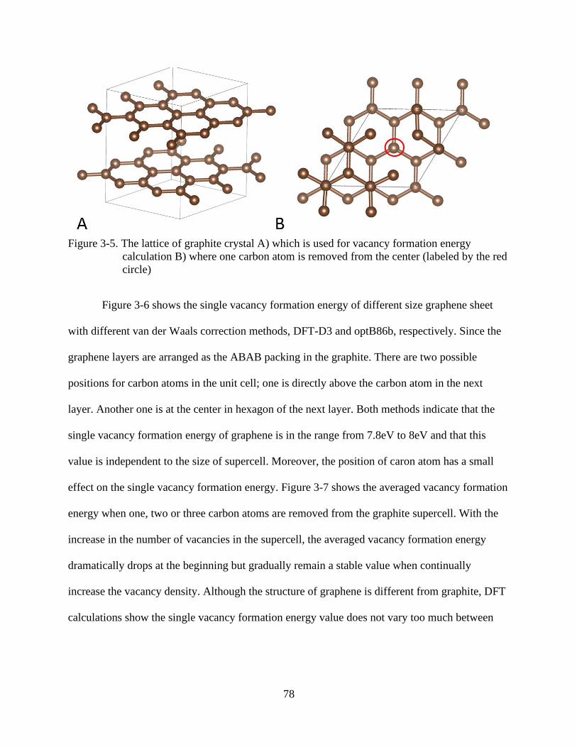
78

Figure 3-5. The lattice of graphite crystal A) which is used for vacancy formation energy

calculation B) where one carbon atom is removed from the center (labeled by the red

circle)

Figure 3-6 shows the single vacancy formation energy of different size graphene sheet

with different van der Waals correction methods, DFT-D3 and optB86b, respectively. Since the

graphene layers are arranged as the ABAB packing in the graphite. There are two possible

positions for carbon atoms in the unit cell; one is directly above the carbon atom in the next

layer. Another one is at the center in hexagon of the next layer. Both methods indicate that the

single vacancy formation energy of graphene is in the range from 7.8eV to 8eV and that this

value is independent to the size of supercell. Moreover, the position of caron atom has a small

effect on the single vacancy formation energy. Figure 3-7 shows the averaged vacancy formation

energy when one, two or three carbon atoms are removed from the graphite supercell. With the

increase in the number of vacancies in the supercell, the averaged vacancy formation energy

dramatically drops at the beginning but gradually remain a stable value when continually

increase the vacancy density. Although the structure of graphene is different from graphite, DFT

calculations show the single vacancy formation energy value does not vary too much between

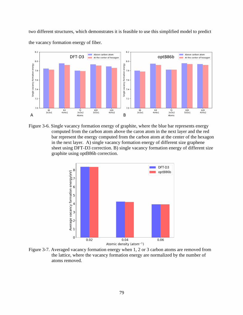
79

two different structures, which demonstrates it is feasible to use this simplified model to predict

the vacancy formation energy of fiber.

Figure 3-6. Single vacancy formation energy of graphite, where the blue bar represents energy

computed from the carbon atom above the caron atom in the next layer and the red

bar represent the energy computed from the carbon atom at the center of the hexagon

in the next layer. A) single vacancy formation energy of different size graphene

sheet using DFT-D3 correction. B) single vacancy formation energy of different size

graphite using optB86b correction.

Figure 3-7. Averaged vacancy formation energy when 1, 2 or 3 carbon atoms are removed from

the lattice, where the vacancy formation energy are normalized by the number of

atoms removed.

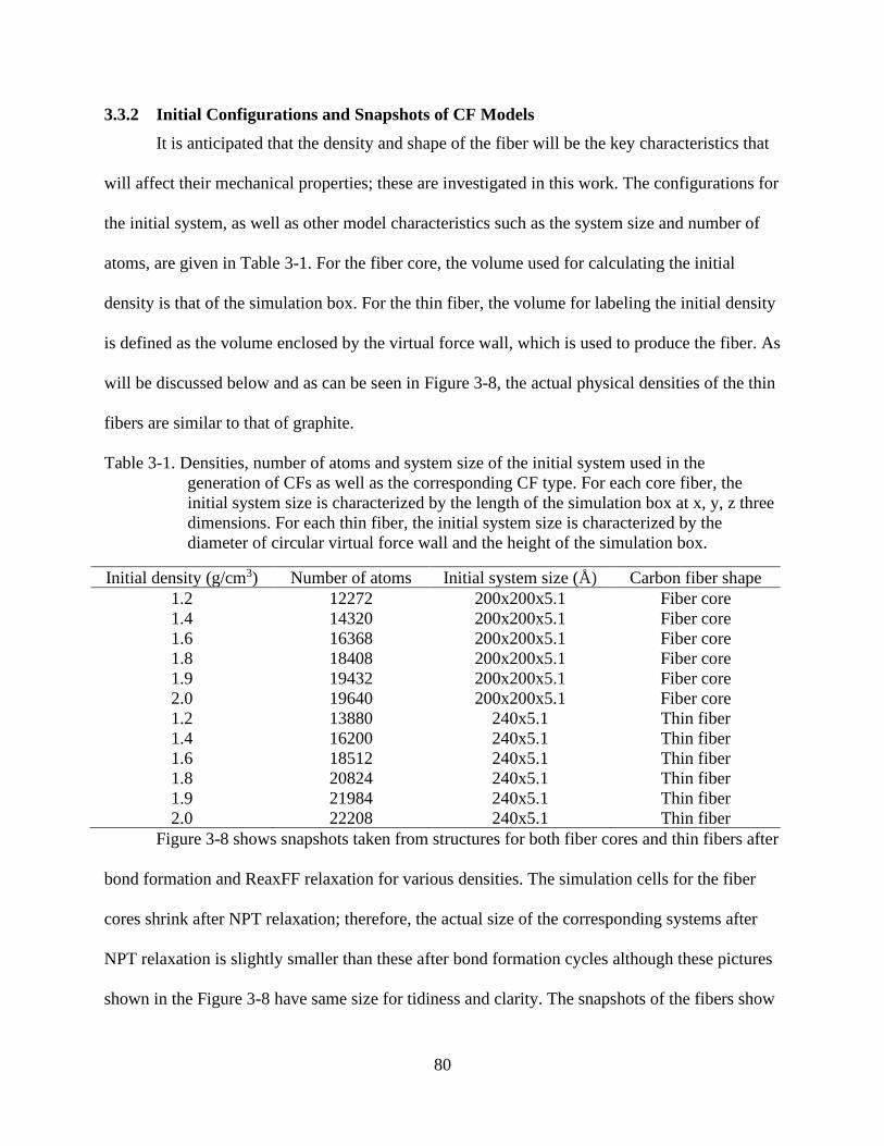
80

3.3.2 Initial Configurations and Snapshots of CF Models

It is anticipated that the density and shape of the fiber will be the key characteristics that

will affect their mechanical properties; these are investigated in this work. The configurations for

the initial system, as well as other model characteristics such as the system size and number of

atoms, are given in Table 3-1. For the fiber core, the volume used for calculating the initial

density is that of the simulation box. For the thin fiber, the volume for labeling the initial density

is defined as the volume enclosed by the virtual force wall, which is used to produce the fiber. As

will be discussed below and as can be seen in Figure 3-8, the actual physical densities of the thin

fibers are similar to that of graphite.

Table 3-1. Densities, number of atoms and system size of the initial system used in the

generation of CFs as well as the corresponding CF type. For each core fiber, the

initial system size is characterized by the length of the simulation box at x, y, z three

dimensions. For each thin fiber, the initial system size is characterized by the

diameter of circular virtual force wall and the height of the simulation box.

Initial density (g/cm3) Number of atoms Initial system size (Å) Carbon fiber shape

1.2 12272 200x200x5.1 Fiber core

1.4 14320 200x200x5.1 Fiber core

1.6 16368 200x200x5.1 Fiber core

1.8 18408 200x200x5.1 Fiber core

1.9 19432 200x200x5.1 Fiber core

2.0 19640 200x200x5.1 Fiber core

1.2 13880 240x5.1 Thin fiber

1.4 16200 240x5.1 Thin fiber

1.6 18512 240x5.1 Thin fiber

1.8 20824 240x5.1 Thin fiber

1.9 21984 240x5.1 Thin fiber

2.0 22208 240x5.1 Thin fiber

Figure 3-8 shows snapshots taken from structures for both fiber cores and thin fibers after

bond formation and ReaxFF relaxation for various densities. The simulation cells for the fiber

cores shrink after NPT relaxation; therefore, the actual size of the corresponding systems after

NPT relaxation is slightly smaller than these after bond formation cycles although these pictures

shown in the Figure 3-8 have same size for tidiness and clarity. The snapshots of the fibers show

81

that, with increasing initial density, the initial structure of both the fiber core and the thin fiber

have more uniform structures and fewer and smaller pores. Comparing the microstructures

generated after bond formation, both corresponding core fiber and thin fiber samples keep

approximately the structure periodicity along the z axis and have similar shapes after ReaxFF

relaxations.

1.2 g/cm3 1.4 g/cm3 1.6 g/cm3 1.8 g/cm3 1.9 g/cm3 2.0 g/cm3

Co

re f

iber

After bond formation cycles

After ReaxFF relaxation

Th

in f

iber

After bond formation cycles

After ReaxFF relaxation

Figure 3-8. Atomistic snapshots of fiber core and thin fiber microstructures after bond formation

cycles and ReaxFF relaxation with various initial densities from 1.2 g/cm3 to 2.0

g/cm3. All snapshots are top views of CF microstructures and all carbon atoms are

colored as green.

82

3.3.3 Shapes, Densities, and Pores

An important structural feature that influences CF properties is the presence of pores

inside the fiber. Therefore, in this section we analyze the final density, the size and distribution

of pores, and the shape of the CFs.

Figure 3-9 compares the initial and final densities of fiber cores and thin fibers. As shown

in Figure 6, all fiber core and thin fiber structures lie above the green dash line, indicating that

they are all densified after the generation process. The final structures of the fiber cores are

denser by 0.1-0.2 g/cm3 after the generation process. By contrast, all of the thin fibers have

essentially the same final densities (in the range 2.16-2.19 g/cm3) after step 4. Some of the fiber

cores have final densities in the experimental range of 1.75-2.0 g/cm3 for PAN fibers[112],

while others are lower. However, thin fiber models have similar final density regardless of the

initial densities. These values are similar to the density range of 1.9-2.2 g/cm3 of pitch-based

carbon fiber[96] and close to graphite’s density of 2.236 g/cm3 [112].

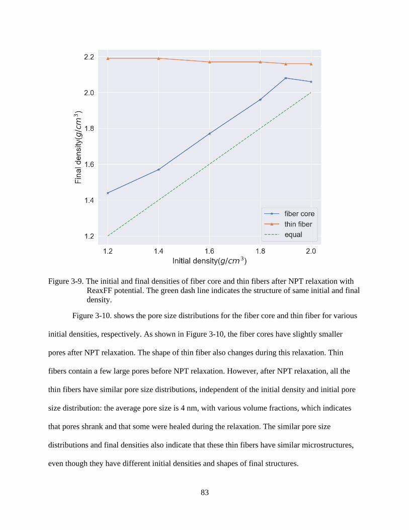
83

Figure 3-9. The initial and final densities of fiber core and thin fibers after NPT relaxation with

ReaxFF potential. The green dash line indicates the structure of same initial and final

density.

Figure 3-10. shows the pore size distributions for the fiber core and thin fiber for various

initial densities, respectively. As shown in Figure 3-10, the fiber cores have slightly smaller

pores after NPT relaxation. The shape of thin fiber also changes during this relaxation. Thin

fibers contain a few large pores before NPT relaxation. However, after NPT relaxation, all the

thin fibers have similar pore size distributions, independent of the initial density and initial pore

size distribution: the average pore size is 4 nm, with various volume fractions, which indicates

that pores shrank and that some were healed during the relaxation. The similar pore size

distributions and final densities also indicate that these thin fibers have similar microstructures,

even though they have different initial densities and shapes of final structures.

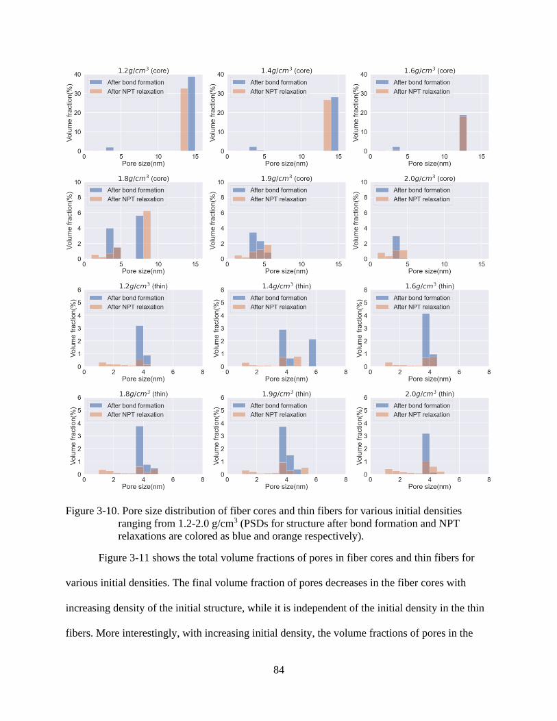
84

Figure 3-10. Pore size distribution of fiber cores and thin fibers for various initial densities

ranging from 1.2-2.0 g/cm3 (PSDs for structure after bond formation and NPT

relaxations are colored as blue and orange respectively).

Figure 3-11 shows the total volume fractions of pores in fiber cores and thin fibers for

various initial densities. The final volume fraction of pores decreases in the fiber cores with

increasing density of the initial structure, while it is independent of the initial density in the thin

fibers. More interestingly, with increasing initial density, the volume fractions of pores in the

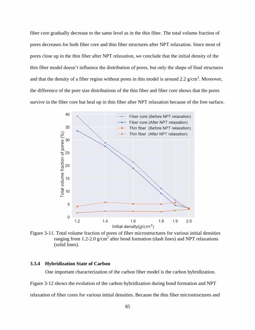
85

fiber core gradually decrease to the same level as in the thin fiber. The total volume fraction of

pores decreases for both fiber core and thin fiber structures after NPT relaxation. Since most of

pores close up in the thin fiber after NPT relaxation, we conclude that the initial density of the

thin fiber model doesn’t influence the distribution of pores, but only the shape of final structures

and that the density of a fiber region without pores in this model is around 2.2 g/cm3. Moreover,

the difference of the pore size distributions of the thin fiber and fiber core shows that the pores

survive in the fiber core but heal up in thin fiber after NPT relaxation because of the free surface.

Figure 3-11. Total volume fraction of pores of fiber microstructures for various initial densities

ranging from 1.2-2.0 g/cm3 after bond formation (dash lines) and NPT relaxations

(solid lines).

3.3.4 Hybridization State of Carbon

One important characterization of the carbon fiber model is the carbon hybridization.

Figure 3-12 shows the evolution of the carbon hybridization during bond formation and NPT

relaxation of fiber cores for various initial densities. Because the thin fiber microstructures and

86

the fiber cores undergo similar evolutions, here we only show and analyze the hybridization

changes for fiber core samples. Beginning with the initial structures described in the Section

3.3.2, the unsaturated sp hybridized carbon atoms from different ladder units bonded with each

other forming sp2 bonds, or in a few cases sp3 bonds, hybridized. The sharp decrease of the sp

population and increase of sp2 population in Figure 3-12 A. and B. show that most of the reactive

sp carbon atoms link with each other in the first 500ps, especially for high initial density

structures such as 1.9 and 2.0 g/cm3. For high initial density structures, the average distance

between unsaturated carbon atoms is smaller, which results in the distance cutoff requirement

being easier to meet so that C-C bonds are easier to created and hybridization is increased.

Therefore, the slopes of sp and sp2 population at initial stage of bond formation are steeper for

high initial density structures. The higher initial density also results in the ladder units not having

enough space to adjust their position during the graphitization process, which lowers the

probability of bond creation. For these two reasons, the 2.0 g/cm3 sample has a very sharp

increase in the number of sp2 bonds at the beginning of the bond formation. Compared with

microstructures of other initial densities, both fiber core and thin fiber structures at 2.0 g/cm3

shows a uniform, almost pore-free microstructure, as shown in Figure 3-8. This is a result of the

ladder unit having little space in which to reorient, resulting in a lower population of sp2

hybridization after bond formation. Except for the 2.0 g/cm3 initial structure, which has a

relatively higher sp population, all other structures reach similar sp and sp2 populations after

bond formation. Figure 3-12 C. and D. show the sp and sp2 population change during NPT

relaxations for fiber cores of various densities. Since the bond creation is explicitly managed by

the kMC-MD algorithm, there is no sp3 population generated during the graphitization process.

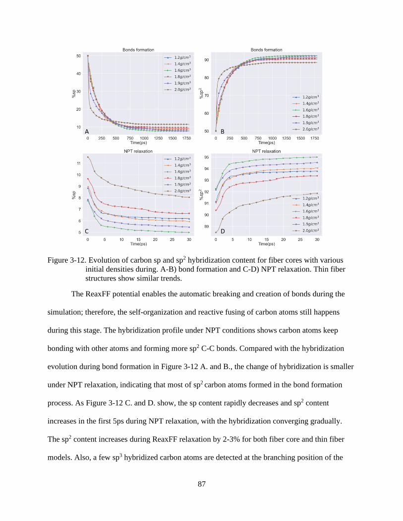
87

Figure 3-12. Evolution of carbon sp and sp2 hybridization content for fiber cores with various

initial densities during. A-B) bond formation and C-D) NPT relaxation. Thin fiber

structures show similar trends.

The ReaxFF potential enables the automatic breaking and creation of bonds during the

simulation; therefore, the self-organization and reactive fusing of carbon atoms still happens

during this stage. The hybridization profile under NPT conditions shows carbon atoms keep

bonding with other atoms and forming more sp2 C-C bonds. Compared with the hybridization

evolution during bond formation in Figure 3-12 A. and B., the change of hybridization is smaller

under NPT relaxation, indicating that most of sp2 carbon atoms formed in the bond formation

process. As Figure 3-12 C. and D. show, the sp content rapidly decreases and sp2 content

increases in the first 5ps during NPT relaxation, with the hybridization converging gradually.

The sp2 content increases during ReaxFF relaxation by 2-3% for both fiber core and thin fiber

models. Also, a few sp3 hybridized carbon atoms are detected at the branching position of the

88

graphitic sheets during ReaxFF relaxations. All samples, other than the 2.0 g/cm3 sample, have

similar sp3 hybridization percentages: about 0.03%. The sp3 concentration in the 2.0 g/cm3

sample is 0.1%, which is still a very small amount compared with the concentration of sp and sp2

boned atoms. As discussed above, the high initial density of these samples prevents the

microstructure from evolving due to minimal amount of space available for ladder units to adjust

their positions. Low initial density also makes the distance between unsaturated carbon atoms

larger than the cutoff and decreases the percentage of sp2 bonds formed. As a result, the sp2

hybridization reaches a maximum for an initial density of 1.6 g/cm3.

3.3.5 XRD Analysis

The structures of the simulated carbon fiber models can be analyzed through their XRD

patterns; this also enables a direct comparison of key microstructural features, such as interplanar

spacing, with experimental results. Again, we only analyze the XRD patterns of the fiber cores

because the thin fiber models show similar behavior. The indexing notation we used in Figure

3-13 follows that in Ref. [121], in which the (100) planes are stacked in the zigzag direction and

the (110) planes are stacked in the armchair direction of the basal planes of the graphitic sheets.

Figure 3-13 A. shows the calculated virtual XRD profile of fiber core structures of

various initial densities, which are presented as stacked curves for clearer representation. All

structures, regardless of initial density, have peaks of almost the same intensities at identical

positions, except the 2.0 g/cm3 structure which has a slightly broad and less intense peak at 2휃 =

27°. Figure 3-13 A. thus shows that the initial density doesn’t have a strong influence on the

structure. Figure 3-13 B. shows the XRD patterns taken from the 1.2 g/cm3 core fiber model

before and after NPT relaxations. The first peak occurs near 2휃 = 27° and corresponds to the

interplanar spacing (d002) in graphite and can be attributed to the graphitic region in the carbon

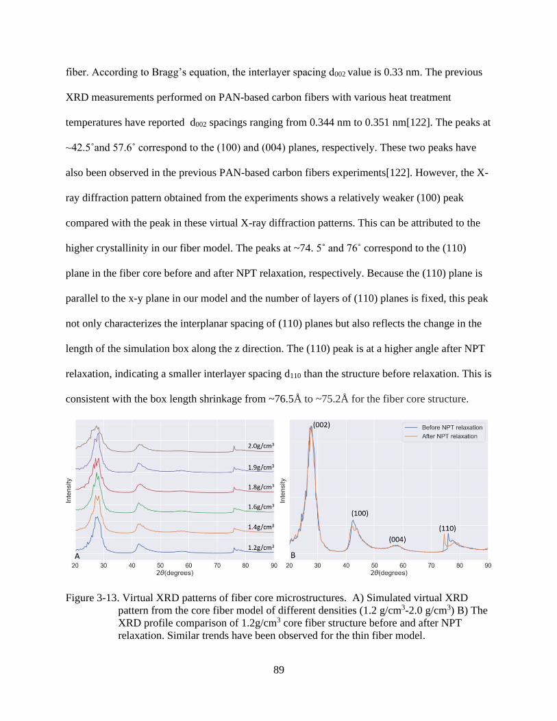
89

fiber. According to Bragg’s equation, the interlayer spacing d002 value is 0.33 nm. The previous

XRD measurements performed on PAN-based carbon fibers with various heat treatment

temperatures have reported d002 spacings ranging from 0.344 nm to 0.351 nm[122]. The peaks at

~42.5˚and 57.6˚ correspond to the (100) and (004) planes, respectively. These two peaks have

also been observed in the previous PAN-based carbon fibers experiments[122]. However, the X-

ray diffraction pattern obtained from the experiments shows a relatively weaker (100) peak

compared with the peak in these virtual X-ray diffraction patterns. This can be attributed to the

higher crystallinity in our fiber model. The peaks at ~74. 5˚ and 76˚ correspond to the (110)

plane in the fiber core before and after NPT relaxation, respectively. Because the (110) plane is

parallel to the x-y plane in our model and the number of layers of (110) planes is fixed, this peak

not only characterizes the interplanar spacing of (110) planes but also reflects the change in the

length of the simulation box along the z direction. The (110) peak is at a higher angle after NPT

relaxation, indicating a smaller interlayer spacing d110 than the structure before relaxation. This is

consistent with the box length shrinkage from ~76.5Å to ~75.2Å for the fiber core structure.

Figure 3-13. Virtual XRD patterns of fiber core microstructures. A) Simulated virtual XRD

pattern from the core fiber model of different densities (1.2 g/cm3-2.0 g/cm3) B) The

XRD profile comparison of 1.2g/cm3 core fiber structure before and after NPT

relaxation. Similar trends have been observed for the thin fiber model.

90

Both the highly ordered graphitic sheets shown in the atomistic snapshots in Figure 3-8

and the sharp XRD peaks in Figure 3-13 result directly from the presence of graphitic crystallites

in the fiber core and thin fiber models. The average size of these crystallites can be estimated

from the X-ray diffraction pattern using Scherrer equation:

𝐿(ℎ𝑘𝑙) =𝐾𝜆

𝐵(2휃) ⋅ 𝑐𝑜𝑠휃 (4-2)

where 𝜆=0.154 nm is the wavelength of the X-rays, 휃 is the diffraction peak 𝐵(2휃) of the (ℎ𝑘𝑙)

plane, 𝐵(2휃) is the full width at the half maximum (FWHM) of the diffraction peak and 𝐾 is

shape factor which varies with the type of crystal structure. Two values are often used to

describe the size of microstructure. The crystallite thickness (𝐿𝑐), which is the average size

perpendicular to the graphitic sheets, is calculated from the (002) diffraction peak. The crystallite

correlation length (𝐿𝑎) along graphitic sheets can be subdivided into 𝐿𝑎∥ parallel with the fiber

axis and 𝐿𝑎⊥ perpendicular to the fiber axis. 𝐿𝑎∥ and 𝐿𝑎⊥ are associated with (100) and (110)

planes, respectively, and can be determined from the corresponding peaks in the diffraction

pattern. The shape factor 𝐾 is 0.89 and 1.84 for 𝐿𝑐 and 𝐿𝑎, respectively[123]. Since the graphitic

sheets in CF models are highly aligned along the fiber axis, the 𝐿𝑎∥ of CF models are determined

by the length of the simulation cell.

Previous experimental studies[123–125] have reported the 𝐿𝑐 for PAN-based carbon fiber

varies over the range 1.6-7.8 nm. Although the experimental values of 𝐿𝑐 vary widely because of

the different processing treatments, the values thus obtained for both core fiber and thin fiber

structures after NPT relaxation show that the generated microstructures have relatively small and

similar crystallite size and correlation length, which lie within the range of the experimental

values. Both core and thin fiber shows a lower 𝐿𝑐 value for microstructures of 2.0 g/cm3 initial

density compared with samples of other initial densities. Similar to the analysis in the Section

91

3.3.4, the high initial density hampered the combination and growth of graphic crystallites,

which caused the low average graphite crystallite size compared with low initial-density

microstructures. The obtained 𝐿𝑎⊥ value is ~13-16nm nm using Scherrer equation, which is

higher than the experimental value, ranging from 5-8.4 nm[125]. Similarly, an 𝐿𝑎⊥ value of ~16

nm is also reported in Desai’s simulation. This overestimation of 𝐿𝑎⊥ can be attributed to the

perfect alignment of fibers along the fiber axis in the model. In a real carbon fiber, the long

chains are not straight and deviate from the fiber axis. The probability of higher random

crosslinking between chains in experiments can also prevent the formation of long graphitic

sheets. Overall, we conclude that the generated microstructures have diffraction patterns that are

similar to each other and are similar in many respects to those of PAN-based CFs. Moreover, the

fiber core and thin fiber have similar diffraction patterns, indicating that the shape does not

influence the characteristics of the generated microstructures. The shift of (110) peaks in the

XRD profiles shows the decrease of interplane spacing of (110) plane after NPT relaxation.

Table 3-2. Average crystallite size of fiber cores and thin fibers for various initial densities.

Initial density(g/cm3) 1.2 1.4 1.6 1.8 1.9 2.0

𝐿𝑐(nm) (Fiber core) 2.29 2.16 2.45 2.84 2.26 1.55

𝐿𝑐(nm) (Thin fiber) 2.09 2.56 2.35 2.13 2.06 1.67

3.3.6 Mechanical Properties

In this section, we investigate the mechanical behavior of the CF using the discontinuous

carbon fiber model. Of course, this CF model is still much simpler than real CFs. Previous study

shows that the high strength PAN-based fiber is composed of carbon micro crystallites[126].

These turbostratic graphitic crystallites are poorly oriented but lie preferentially parallel to the

92

fiber axis. The simulated crystallites of models are still highly parallel to the fiber axis.

Moreover, crystallites in realistic fibers can twist, interweave, and fold with other crystallites,

and are accompanied by dislocations, micro voids and amorphous non graphitic carbon

regions[127,128]. XRD and Raman spectroscopy reported that an amorphous region exist in the

in CF, in which carbon atoms are mainly sp2 hybridized and form cross-linked, non-aligned

sheets[129]. Using the Mori-Tanaka’s mean stress method, Ishikawa et al. reported that the

torsional modulus is impacted by the volume of the amorphous [130,131]. Thus, a realistic

carbon fiber is much more complicated and much more disordered than the simulated models.

Due to the nature of the simulation method and the replication along the fiber direction, there are

no misoriented graphitic sheets along the z-direction. The graphitic region is characterized using

the criteria proposed by Joshi[98]: (1) The energy of a carbon atom is ~30 meV/atom, and (2) the

carbon atoms are in the sp2 hybridization state. We find only a few carbon atoms at the edge of

the graphite sheet that do not meet this criterion; these have high energy due to their

undercoordination. Since all of these microstructural defects and amorphous regions in CF are

likely to reduce the mechanical integrity of the experimental systems, the current CF models can

be expected to be stronger than real CFs. Therefore, one line of carbon atoms is removed at a

random position in each graphitic sheet in the discontinuous model to mimic the presence of

defects along the fiber axis. However, this is offset by the very short lengths of the graphitic

sheets in the computational models, 76.5 Å, which is substantially less than the experimental

values at order of micrometers[132], and likely to make the computational models much more

susceptible to the pullout mechanism, described below, than their experimental counterparts.

We observed that some of the artificial breaks in the model graphitic sheets heal during

the structural equilibration: this increases the mechanical integrity of the system. In order to

93

quantify the healing of the broken sheets, we tracked the change of the average width of the

breaks between the upper and lower parts of what was originally a single sheet. To investigate

the influence of the break width, we removed one, two or three layers of carbon atoms in each

sheet. Interestingly, we found the fiber model is independent of the width of breaks: as shown in

Figure 3-14 A., the breaks healed to the same average width. Although wider breaks need more

time to heal, all sample healed within 2 ps and the structure remained stable throughout the rest

of the simulation. Moreover, it showed that there are still some breaks after re-healing, although

the gap width is substantially lowered, and partial breaks disappear. Figure 3-14 B. shows the

width distribution of breaks of different initial width for 1.8g/cm3 fiber core after the healing

processes. Since three distributions with different initial gap width in Figure 3-14 A. show

similar patterns, it is evident that the initial width has a weak influence on the final width

distribution. No matter what the initial widths of the breaks are, the breaks partially heal to same

final width, which corresponds well with the finding in the Figure 3-14 A. that the average break

width is nearly independent to the initial width after re-healing. Moreover, Figure 3-14 B. shows

some gaps are healed and have width less than 1.8Å, the bond cutoff in the ReaxFF potential,

indicating that some covalent bonds are recreated between carbon atoms at the edge of the gap.

Therefore, in the tensile simulation, bond breaking still determines the tensile strength but is

greatly weakened by the relatively low density of such strong bonds. Figure 3-14 C. shows that

the break width increases linearly with tensile strain, which can be attributed to the linear

deformation of the simulation cell as function of time in the loading process. Figure 3-14 D.

shows the stress-strain curves of 1.8 g/cm3 fiber core models with different initial break widths.

As shown in Figure 3-14 A., since the width of the average break is almost the same after the re-

healing process, samples should have similar defects features. The three almost identical and

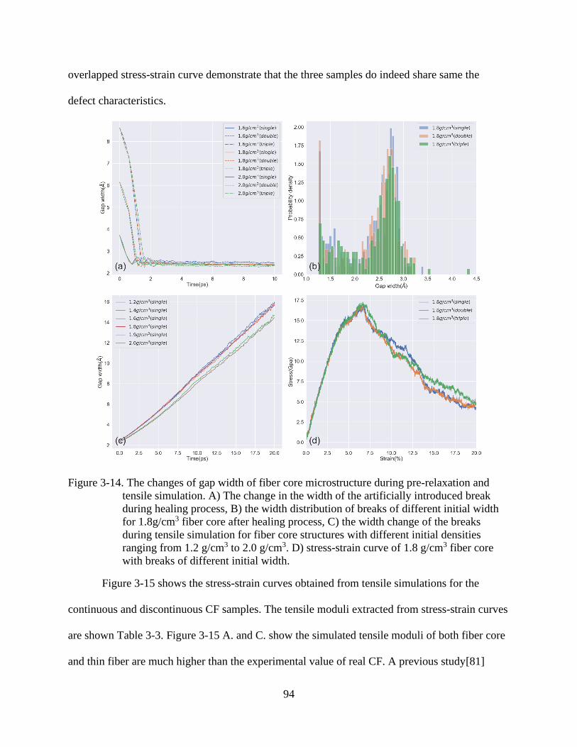
94

overlapped stress-strain curve demonstrate that the three samples do indeed share same the

defect characteristics.

Figure 3-14. The changes of gap width of fiber core microstructure during pre-relaxation and

tensile simulation. A) The change in the width of the artificially introduced break

during healing process, B) the width distribution of breaks of different initial width

for 1.8g/cm3 fiber core after healing process, C) the width change of the breaks

during tensile simulation for fiber core structures with different initial densities

ranging from 1.2 g/cm3 to 2.0 g/cm3. D) stress-strain curve of 1.8 g/cm3 fiber core

with breaks of different initial width.

Figure 3-15 shows the stress-strain curves obtained from tensile simulations for the

continuous and discontinuous CF samples. The tensile moduli extracted from stress-strain curves

are shown Table 3-3. Figure 3-15 A. and C. show the simulated tensile moduli of both fiber core

and thin fiber are much higher than the experimental value of real CF. A previous study[81]

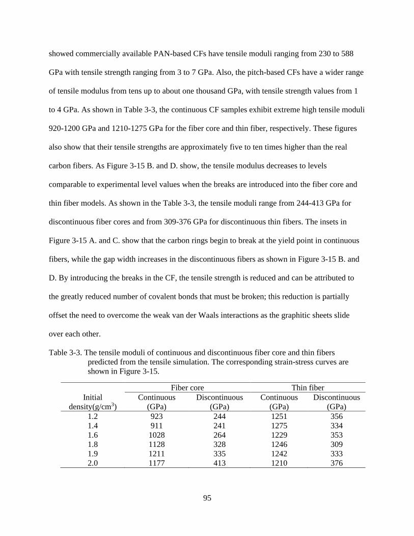
95

showed commercially available PAN-based CFs have tensile moduli ranging from 230 to 588

GPa with tensile strength ranging from 3 to 7 GPa. Also, the pitch-based CFs have a wider range

of tensile modulus from tens up to about one thousand GPa, with tensile strength values from 1

to 4 GPa. As shown in Table 3-3, the continuous CF samples exhibit extreme high tensile moduli

920-1200 GPa and 1210-1275 GPa for the fiber core and thin fiber, respectively. These figures

also show that their tensile strengths are approximately five to ten times higher than the real

carbon fibers. As Figure 3-15 B. and D. show, the tensile modulus decreases to levels

comparable to experimental level values when the breaks are introduced into the fiber core and

thin fiber models. As shown in the Table 3-3, the tensile moduli range from 244-413 GPa for

discontinuous fiber cores and from 309-376 GPa for discontinuous thin fibers. The insets in

Figure 3-15 A. and C. show that the carbon rings begin to break at the yield point in continuous

fibers, while the gap width increases in the discontinuous fibers as shown in Figure 3-15 B. and

D. By introducing the breaks in the CF, the tensile strength is reduced and can be attributed to

the greatly reduced number of covalent bonds that must be broken; this reduction is partially

offset the need to overcome the weak van der Waals interactions as the graphitic sheets slide

over each other.

Table 3-3. The tensile moduli of continuous and discontinuous fiber core and thin fibers

predicted from the tensile simulation. The corresponding strain-stress curves are

shown in Figure 3-15.

Fiber core Thin fiber

Initial

density(g/cm3)

Continuous

(GPa)

Discontinuous

(GPa)

Continuous

(GPa)

Discontinuous

(GPa)

1.2 923 244 1251 356

1.4 911 241 1275 334

1.6 1028 264 1229 353

1.8 1128 328 1246 309

1.9 1211 335 1242 333

2.0 1177 413 1210 376

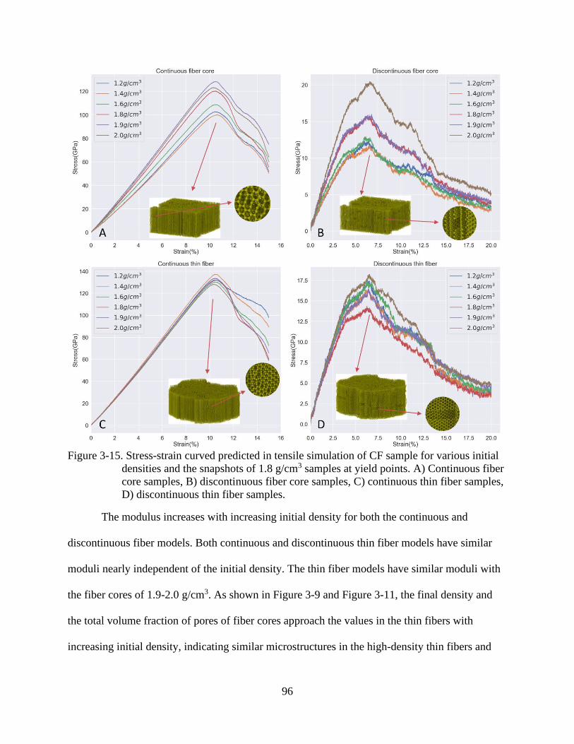
96

Figure 3-15. Stress-strain curved predicted in tensile simulation of CF sample for various initial

densities and the snapshots of 1.8 g/cm3 samples at yield points. A) Continuous fiber

core samples, B) discontinuous fiber core samples, C) continuous thin fiber samples,

D) discontinuous thin fiber samples.

The modulus increases with increasing initial density for both the continuous and

discontinuous fiber models. Both continuous and discontinuous thin fiber models have similar

moduli nearly independent of the initial density. The thin fiber models have similar moduli with

the fiber cores of 1.9-2.0 g/cm3. As shown in Figure 3-9 and Figure 3-11, the final density and

the total volume fraction of pores of fiber cores approach the values in the thin fibers with

increasing initial density, indicating similar microstructures in the high-density thin fibers and

97

fiber cores. Moreover, unlike the fiber core, the thin fiber is non-periodic in the x-y plane.

Because the graphitic sheets at the outer surface of the thin fiber only interact with one side of

other graphitic sheets via van der Waals force, pullout of these fibers is easier than in the

interior[133]. Due to the periodic conditions, all the graphitic sheets in fiber core interact with

two sides of other sheets via van der Waals interactions, which makes the system stronger.

Therefore, although thin fibers have similar densities as the fiber core, the tensile modulus is still

slightly lower. It is worth noting that the tensile strength of the discontinuous carbon fiber model

is still 2-5 times larger than the experimental value. As discussed at the beginning of this section,

the strength of real fibers is further reduced by the misorientation, defects, amorphous regions,

and micro-voids along the longitudinal direction, which are not captured in this model.

Moreover, the high level of alignment along the axis in our fiber model increases the tensile

strength.

The transverse moduli of CFs are also computed by conducting tensile simulations in

direction normal to the fiber direction. Since there is empty space surrounding the thin fiber, we

only compute the transverse modulus of fiber core model. The transverse modulus of CFs has

been experimentally evaluated by tensile compression tests[134], showing that the transverse

moduli of pitch based and PAN based CFs range from 1 to 4 GPa, while the moduli of some high

strength PAN based CFs can be up to 9 GPa.

Figure 3-16 A. shows that the transverse moduli of fiber cores range from 0.2 GPa to 4.5

GPa, which agrees well with experimental result. Since the transverse modulus can be influenced

by the alignment direction of graphitic sheets, the modulus along both the X and Y direction is

calculated. As the density increases, the modulus generally increases. For the low-density carbon

fibers, there are large pores in the fiber core structure which decrease the contact area between

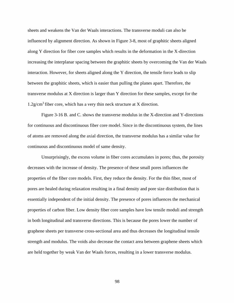
98

sheets and weakens the Van der Waals interactions. The transverse moduli can also be

influenced by alignment direction. As shown in Figure 3-8, most of graphitic sheets aligned

along Y direction for fiber core samples which results in the deformation in the X-direction

increasing the interplanar spacing between the graphitic sheets by overcoming the Van der Waals

interaction. However, for sheets aligned along the Y direction, the tensile force leads to slip

between the graphitic sheets, which is easier than pulling the planes apart. Therefore, the

transverse modulus at X direction is larger than Y direction for these samples, except for the

1.2g/cm3 fiber core, which has a very thin neck structure at X direction.

Figure 3-16 B. and C. shows the transverse modulus in the X-direction and Y-directions

for continuous and discontinuous fiber core model. Since in the discontinuous system, the lines

of atoms are removed along the axial direction, the transverse modulus has a similar value for

continuous and discontinuous model of same density.

Unsurprisingly, the excess volume in fiber cores accumulates in pores; thus, the porosity

decreases with the increase of density. The presence of these small pores influences the

properties of the fiber core models. First, they reduce the density. For the thin fiber, most of

pores are healed during relaxation resulting in a final density and pore size distribution that is

essentially independent of the initial density. The presence of pores influences the mechanical

properties of carbon fiber. Low density fiber core samples have low tensile moduli and strength

in both longitudinal and transverse directions. This is because the pores lower the number of

graphene sheets per transverse cross-sectional area and thus decreases the longitudinal tensile

strength and modulus. The voids also decrease the contact area between graphene sheets which

are held together by weak Van der Waals forces, resulting in a lower transverse modulus.

99

Figure 3-16. The transverse moduli of fiber core models A) The transverse moduli at X and Y

direction of fiber core of different densities ranging from 1.2-2.0 g/cm3 B-C) The

transverse moduli at X direction and Y direction of continuous and discontinuous

fiber cores of different densities ranging from 1.2-2.0 g/cm3.

3.4 Summary

We have modeled carbon fiber using a kMC-MD algorithm and ReaxFF reactive force

field. The microstructures are generated from initial eight-atom ladder units by creating bonds

between unsaturated carbon atoms of different units based on the kMC-MD algorithm. Then the

generated 2D microstructure is replicated in the z-direction to form fully 3D microstructures and

relaxed by the physically sophisticated ReaxFF reactive force field. Fiber core and thin fiber CF

models are generated by controlling the CF shape via a virtual force wall. These fiber core and

thin fiber models represent a small section of the interior region of thick fiber and a very thin

carbon fiber with a well-defined surface. Extensive characterization of structural features

including initial packing densities, final densities of structures, pore size distribution,

hybridization state, XRD analysis yielded results similar to experimental results in the literature.

Moreover, the mechanical properties of this CF model were investigated, and a discontinuous CF

model was proposed by removing one layer of carbon atoms at random position of each graphitic

sheet; this resulted in a reduction in the tensile modulus to levels comparable to real carbon

fibers. Our key findings are:

100

1. By controlling the initial packing density, the generated fiber core models can have a

large range of the final density from 1.45-2.10 g/cm3. For initial densities up to 1.9 g/cm3,

the final density of fiber increases with the increase of the initial density. The final

density of 2.0 g/cm3 fiber core is slightly lower than the 1.9g/cm3 fiber core. Since the

free surface annihilate most of pores in thin fiber model, the final density of thin fiber

model is independent to the initial packing density and the densities of all thin fiber

samples are densified to the 2.16-2.19 g/cm3 after generation process.

2. The pore size distribution analysis shows the volume fractions of pores decreased in fiber

core with the increase of the density of the initial structure while it is independent to the

initial density in thin fiber.

3. Both core fiber and thin fiber models show similar evolution of hybridization state during

the generation process. The percentage of sp hybridization decreases to below 10% while

it of sp2 hybridization increases to above 90% in the generation. No more than 0.1% sp3

hybridized carbon atoms are observed in both fiber core and thin fibers.

4. XRD analysis results show the crystallite thickness 𝐿𝑐 and crystallite correlation length

𝐿𝑎 obtained from both fiber core and thin fiber models are consistent with experimental

values in the literature, although the average crystallite thickness and correlation length

among fiber models is relatively smaller than experimental values.

5. By introducing physically reasonable discontinuities in the structures the z-direction, the

Young’s modulus of discontinuous fiber core and thins fiber models are in the range of

200-400 GPa, which lies in the modulus range of PAN fiber. However, the tensile

strength of discontinuous model is still 2-5 times larger than the experiment value due to

the high level of alignment and the absence of other structural imperfection in the model.

101

It should be noted that the discontinuous model reaches the axial tensile moduli

comparable with experimental results. However, covalent bonds and the complex

morphologies still dominate the tensile modulus in real fiber. The transverse modulus of

both continuous and discontinuous fiber core models is in the range of 0.2-5 GPa which

agrees well with the experimental value of transverse modulus of PAN and pitched based

CFs.

6. The high-density fiber core has a similar microstructure to the thin fiber because they

have similar final densities. The method presented here is a good first step to the

construction of a highly realistic carbon fiber model. The thin fiber model is an ideal

platform in which to investigate the surface chemical reactions between carbon fibers and

reactive gases, most particularly atomic and molecular oxygen. Since carbon fibers are

also frequently embedded in polymer or metal matrix to form composites, the thin fiber

model also provides an opportunity to investigate the interfacial properties with a matrix

such as resin.

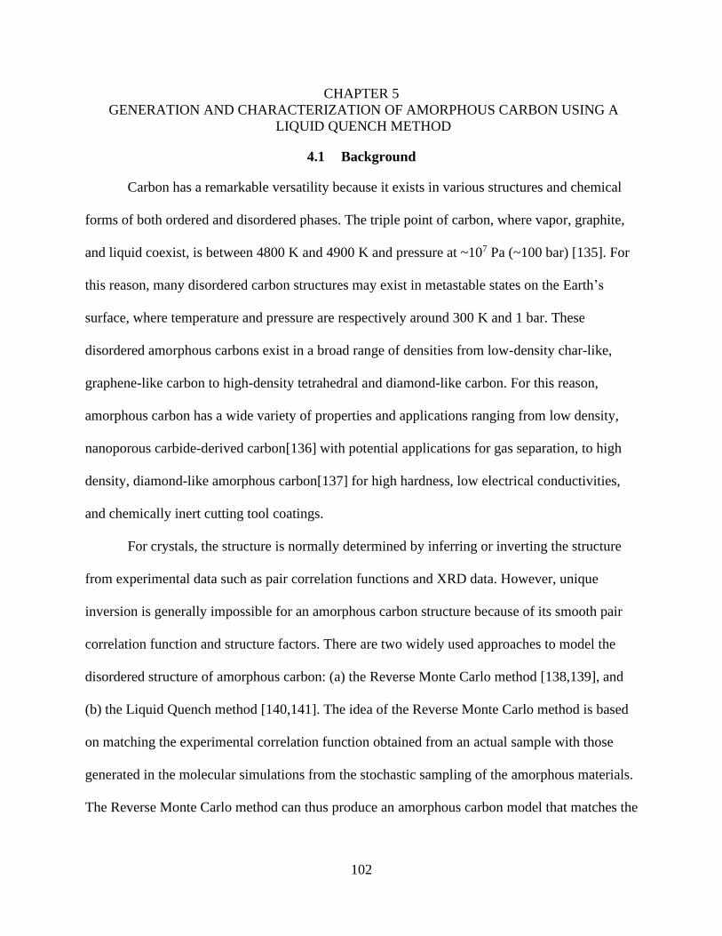
102

CHAPTER 5

GENERATION AND CHARACTERIZATION OF AMORPHOUS CARBON USING A

LIQUID QUENCH METHOD

4.1 Background

Carbon has a remarkable versatility because it exists in various structures and chemical

forms of both ordered and disordered phases. The triple point of carbon, where vapor, graphite,

and liquid coexist, is between 4800 K and 4900 K and pressure at ~107 Pa (~100 bar) [135]. For

this reason, many disordered carbon structures may exist in metastable states on the Earth’s

surface, where temperature and pressure are respectively around 300 K and 1 bar. These

disordered amorphous carbons exist in a broad range of densities from low-density char-like,

graphene-like carbon to high-density tetrahedral and diamond-like carbon. For this reason,

amorphous carbon has a wide variety of properties and applications ranging from low density,

nanoporous carbide-derived carbon[136] with potential applications for gas separation, to high

density, diamond-like amorphous carbon[137] for high hardness, low electrical conductivities,

and chemically inert cutting tool coatings.

For crystals, the structure is normally determined by inferring or inverting the structure

from experimental data such as pair correlation functions and XRD data. However, unique

inversion is generally impossible for an amorphous carbon structure because of its smooth pair

correlation function and structure factors. There are two widely used approaches to model the

disordered structure of amorphous carbon: (a) the Reverse Monte Carlo method [138,139], and

(b) the Liquid Quench method [140,141]. The idea of the Reverse Monte Carlo method is based

on matching the experimental correlation function obtained from an actual sample with those

generated in the molecular simulations from the stochastic sampling of the amorphous materials.

The Reverse Monte Carlo method can thus produce an amorphous carbon model that matches the

103

experimental result (normally the pair correlation result). It is computationally inexpensive and

easy to implement. However, since the relationship between the amorphous structure and the pair

correlation is not uniquely one to one, Reverse Monte Carlo can produce models with incorrect

coordination or chemical order[142]. Therefore, more constraints like multiple scattering data

and bond angle distribution are introduced to resolve this issue.

A quite different method for generating amorphous carbon is to try to mimic or capture

the chemistry of the formation process of amorphous carbon, namely, liquid quench method. In

this method, carbon is quenched from a high temperature liquid to a low temperature solid,

which forms as an amorphous carbon structure. In contrast to the Reverse Monte Carlo method,

the liquid quench method dose not rely on experimental data and can generate some novel

amorphous system that have not been studied experimentally. In this chapter, we focus on using

the liquid quench route developed by Ranganathan[141] to generate and characterize amorphous

carbon structures. We further compare the amorphous structures generated by REBO and

ReaxFF potentials. These results show a reliable way to generate amorphous carbon structures

with a wide range of densities and reveal their important structural features.

4.2 Computational Methods

The amorphous carbon structure investigated in this study is generated by the liquid

quench method that is described in Ranganathan’s work[141]. Liquid quench methods are widely

used to generated and model amorphous carbon[143], monatomic metallic glasses[144] and

carbide-derived carbons[145]. REBO[146] and ReaxFF[104] potentials are used in this work.

Both REBO and ReaxFF are reactive potentials that uses the bond order to automatically manage

the dynamic bond breaking and formation. The parameters of both REBO and ReaxFF potentials

are derived from quantum mechanics and therefore these two potentials can be applied to the

104

novel systems that have not yet been studied in the experiments. Compared with the REBO

potential, the ReaxFF potential has more complex forms of the potential parameters and higher

accuracy but slower computation speed. The overall steps in the liquid quench method are

1. Begin with 𝑁 carbon atoms arranged at the random position in the simulation cell.

2. Equilibrate the system at 10000 K for 15 ps.

3. Quench the system to 3000 K with a constant quench rate 𝑄.

4. Anneal the system at 3000 K for 140 ps.

5. Quench the system to 300 K with the same constant quench rate Q in step 3.

6. Equilibrate the system at 300 K for 10 ps.

In this work, the number of carbon atoms 𝑁 is set to 1200 and the constant quench rate 𝑄 is 50

K/ps. The size of the simulation cell varies with the different densities. The canonical ensemble

with constant volume and a damping constant of 70 fs is used in the simulation. The timestep is

set to 0.07 fs and the volume of simulation cell is fixed during the whole simulation. All

simulations in this chapter are performed using LAMMPS software[103] with “USER-REAXC”

package. Using the REBO potential, amorphous carbon structures with densities from 0.5 g/cm3

to 3.2 g/cm3 are generated; using the ReaxFF potential, amorphous carbon structures with

densities from 0.5 g/cm3 to 2.0 g/cm3 are generated. The amorphous carbon structures are

characterized by structural visualization and detailed analysis including hybridization content,

pair correlation function, bond-angle distribution, ring-size distribution, and pore size

distribution. Ovito[21] and its python interface is used for the visualization and pair correlation

analysis. Issacs[147] and Zeo++[148] software are used for computing the ring-size distribution

and pore sized distribution, respectively.

4.3 Characterization of Amorphous Carbon

In this section, we investigate the structural properties of the amorphous carbon at the

range of densities from 0.5g/cm3 to 3.2g/cm3. Figure 4-1 and Figure 4-2 show snapshots of the

105

final amorphous carbon structure at various densities using REBO and ReaxFF potentials,

respectively. Both REBO and ReaxFF 0.5g/cm3 and 1.0g/cm3 structures are observed to be

highly porous. As the density is increased, the simulation cell gradually fills with the carbon

atoms, thereby generating less and less porous amorphous structures. At 3.2g/cm3 and 2.0g/cm3

for REBO and ReaxFF potentials, the structure is predominantly graphitic, with graphene sheets

parallels stack to each other with additional interplanar bonds. Suarez-Martinez[143] observed

the spontaneously evolution of a graphene-sheet like structure under high temperature annealing

at 2.24g/cm3 and Ranganathan[141] observed the formation of parallel graphitic sheet like

amorphous structure at 2.5g/cm3 using ReaxFF potential by liquid quench method. The 2.0g/cm3

structure using ReaxFF potential shows a similar, but not as well-developed, graphene-like

structure. It is expected to be form clearer a graphene-sheet like structure when the density is

increased to 2.5g/cm3. Ranganathan also observed that a rigid network of tetrahedrally-

coordinated structure, where most of atoms are sp3 hybridized, was generated at 3.2g/cm3 using

the ReaxFF potential. However, we observe that a highly parallelly stacked graphitic sheet like

structure generated using REBO potential at 3.2g/cm3. This structure is similar to that generated

at 2.5g/cm3 using the ReaxFF potential in Ranganathan’s work. The tetrahedrally-coordinated

structure is not observed in the 3.2g/cm3 amorphous carbon structure using REBO potential. We

attribute this difference as arising from the tendency of the REBO potential to generate

graphene-sheet like structured while ReaxFF tends to generate tetrahedrally diamond-like

structures at the high density of 3.2g/cm3.

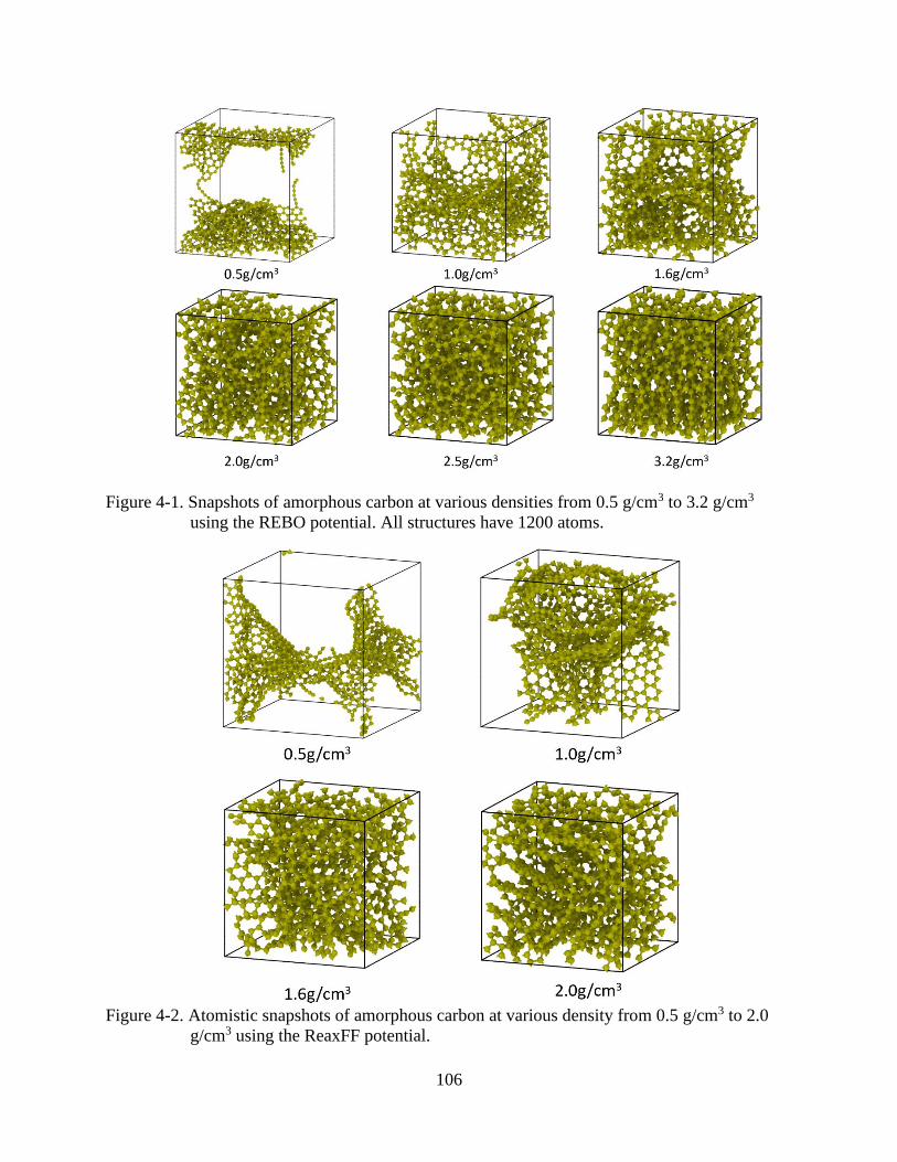
106

Figure 4-1. Snapshots of amorphous carbon at various densities from 0.5 g/cm3 to 3.2 g/cm3

using the REBO potential. All structures have 1200 atoms.

Figure 4-2. Atomistic snapshots of amorphous carbon at various density from 0.5 g/cm3 to 2.0

g/cm3 using the ReaxFF potential.

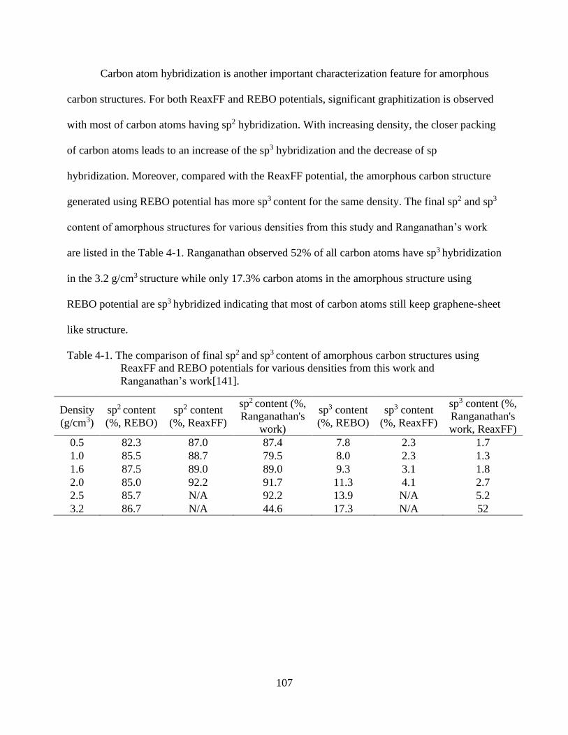
107

Carbon atom hybridization is another important characterization feature for amorphous

carbon structures. For both ReaxFF and REBO potentials, significant graphitization is observed

with most of carbon atoms having sp2 hybridization. With increasing density, the closer packing

of carbon atoms leads to an increase of the sp3 hybridization and the decrease of sp

hybridization. Moreover, compared with the ReaxFF potential, the amorphous carbon structure

generated using REBO potential has more sp3 content for the same density. The final sp2 and sp3

content of amorphous structures for various densities from this study and Ranganathan’s work

are listed in the Table 4-1. Ranganathan observed 52% of all carbon atoms have sp3 hybridization

in the 3.2 g/cm3 structure while only 17.3% carbon atoms in the amorphous structure using

REBO potential are sp3 hybridized indicating that most of carbon atoms still keep graphene-sheet

like structure.

Table 4-1. The comparison of final sp2 and sp3 content of amorphous carbon structures using

ReaxFF and REBO potentials for various densities from this work and

Ranganathan’s work[141].

Density

(g/cm3)

sp2 content

(%, REBO)

sp2 content

(%, ReaxFF)

sp2 content (%,

Ranganathan's

work)

sp3 content

(%, REBO)

sp3 content

(%, ReaxFF)

sp3 content (%,

Ranganathan's

work, ReaxFF)

0.5 82.3 87.0 87.4 7.8 2.3 1.7

1.0 85.5 88.7 79.5 8.0 2.3 1.3

1.6 87.5 89.0 89.0 9.3 3.1 1.8

2.0 85.0 92.2 91.7 11.3 4.1 2.7

2.5 85.7 N/A 92.2 13.9 N/A 5.2

3.2 86.7 N/A 44.6 17.3 N/A 52

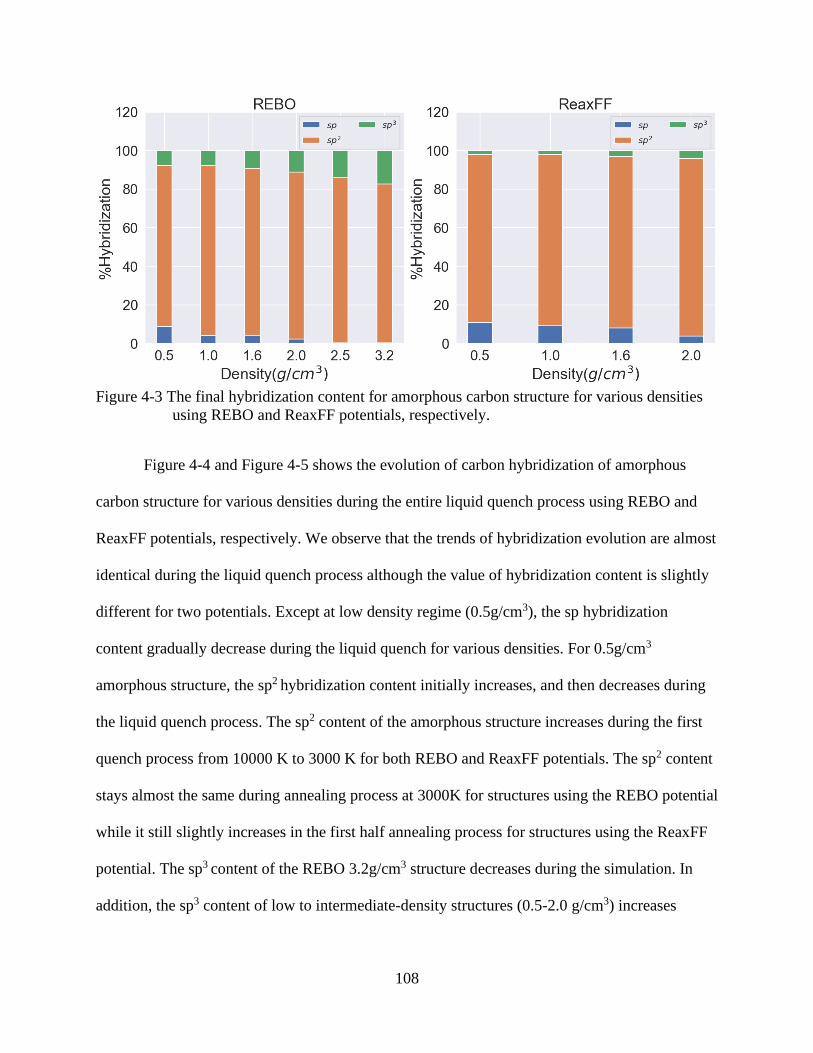
108

Figure 4-3 The final hybridization content for amorphous carbon structure for various densities

using REBO and ReaxFF potentials, respectively.

Figure 4-4 and Figure 4-5 shows the evolution of carbon hybridization of amorphous

carbon structure for various densities during the entire liquid quench process using REBO and

ReaxFF potentials, respectively. We observe that the trends of hybridization evolution are almost

identical during the liquid quench process although the value of hybridization content is slightly

different for two potentials. Except at low density regime (0.5g/cm3), the sp hybridization

content gradually decrease during the liquid quench for various densities. For 0.5g/cm3

amorphous structure, the sp2 hybridization content initially increases, and then decreases during

the liquid quench process. The sp2 content of the amorphous structure increases during the first

quench process from 10000 K to 3000 K for both REBO and ReaxFF potentials. The sp2 content

stays almost the same during annealing process at 3000K for structures using the REBO potential

while it still slightly increases in the first half annealing process for structures using the ReaxFF

potential. The sp3 content of the REBO 3.2g/cm3 structure decreases during the simulation. In

addition, the sp3 content of low to intermediate-density structures (0.5-2.0 g/cm3) increases

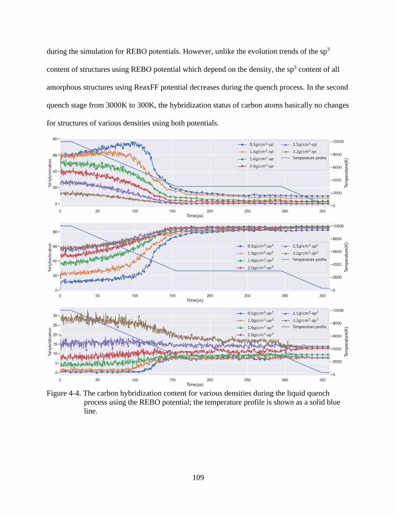
109

during the simulation for REBO potentials. However, unlike the evolution trends of the sp3

content of structures using REBO potential which depend on the density, the sp3 content of all

amorphous structures using ReaxFF potential decreases during the quench process. In the second

quench stage from 3000K to 300K, the hybridization status of carbon atoms basically no changes

for structures of various densities using both potentials.

Figure 4-4. The carbon hybridization content for various densities during the liquid quench

process using the REBO potential; the temperature profile is shown as a solid blue

line.

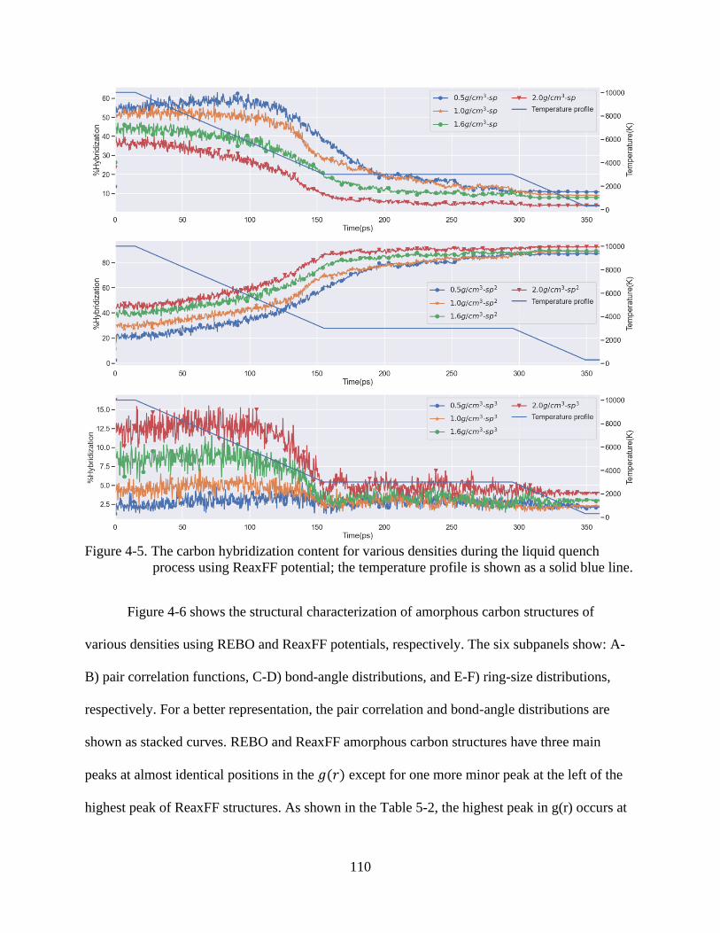
110

Figure 4-5. The carbon hybridization content for various densities during the liquid quench

process using ReaxFF potential; the temperature profile is shown as a solid blue line.

Figure 4-6 shows the structural characterization of amorphous carbon structures of

various densities using REBO and ReaxFF potentials, respectively. The six subpanels show: A-

B) pair correlation functions, C-D) bond-angle distributions, and E-F) ring-size distributions,

respectively. For a better representation, the pair correlation and bond-angle distributions are

shown as stacked curves. REBO and ReaxFF amorphous carbon structures have three main

peaks at almost identical positions in the 𝑔(𝑟) except for one more minor peak at the left of the

highest peak of ReaxFF structures. As shown in the Table 5-2, the highest peak in g(r) occurs at

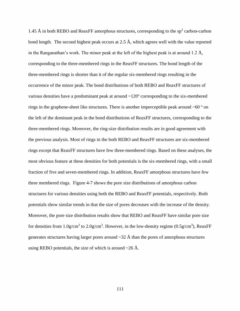
111

1.45 Å in both REBO and ReaxFF amorphous structures, corresponding to the sp2 carbon-carbon

bond length. The second highest peak occurs at 2.5 Å, which agrees well with the value reported

in the Ranganathan’s work. The minor peak at the left of the highest peak is at around 1.2 Å,

corresponding to the three-membered rings in the ReaxFF structures. The bond length of the

three-membered rings is shorter than it of the regular six-membered rings resulting in the

occurrence of the minor peak. The bond distributions of both REBO and ReaxFF structures of

various densities have a predominant peak at around ~120º corresponding to the six-membered

rings in the graphene-sheet like structures. There is another imperceptible peak around ~60 º on

the left of the dominant peak in the bond distributions of ReaxFF structures, corresponding to the

three-membered rings. Moreover, the ring-size distribution results are in good agreement with

the previous analysis. Most of rings in the both REBO and ReaxFF structures are six-membered

rings except that ReaxFF structures have few three-membered rings. Based on these analyses, the

most obvious feature at these densities for both potentials is the six-membered rings, with a small

fraction of five and seven-membered rings. In addition, ReaxFF amorphous structures have few

three membered rings. Figure 4-7 shows the pore size distributions of amorphous carbon

structures for various densities using both the REBO and ReaxFF potentials, respectively. Both

potentials show similar trends in that the size of pores decreases with the increase of the density.

Moreover, the pore size distribution results show that REBO and ReaxFF have similar pore size

for densities from 1.0g/cm3 to 2.0g/cm3. However, in the low-density regime (0.5g/cm3), ReaxFF

generates structures having larger pores around ~32 Å than the pores of amorphous structures

using REBO potentials, the size of which is around ~26 Å.

112

Figure 4-6. Structural characterization of amorphous carbon structures of various densities using

REBO and ReaxFF potentials A-B) Pair correlation functions C-D) bond-angle

distribution E-F) ring-size distribution. The pair correlation and bond-angle

distribution functions are shown as stacked curves for a better representation.

113

Figure 4-7. The pore size distributions of amorphous carbon structures for various densities using

REBO and ReaxFF potentials, respectively.

Table 4-2. List of values of peak (P) and its positions (R) of pair correlation functions of

amorphous carbon structures for various densities using REBO and ReaxFF

potentials

Density(g/cm3) R1(Å) P1 R2(Å) P2 R3(Å) P3

RE

BO

0.5 1.42 40.52 2.42 12.80 3.74 5.57

1.0 1.43 21.51 2.47 6.57 3.77 3.01

1.6 1.44 11.96 2.47 4.29 3.68 1.77

2.0 1.45 9.48 2.47 3.34 3.71 1.48

2.5 1.44 7.09 2.47 2.79 3.66 1.43

3.2 1.42 6.33 2.50 2.73 3.73 1.41

Rea

xF

F

0.5 1.45 68.87 2.52 13.09 3.82 5.72

1.0 1.45 36.47 2.49 6.34 3.76 3.07

1.6 1.46 21.89 2.50 4.42 3.83 1.89

2.0 1.46 16.53 2.52 3.14 3.81 1.85

114

4.4 Summary

In this chapter, we generate amorphous carbon structures for a wide range of densities by

liquid quench method using REBO and ReaxFF potentials. The structural features of the

amorphous structures are characterized by analyses of the structure visualization, hybridization,

pair correlation function, bond-angle distribution, ring-size distribution, and pore size

distributions. Our results show that, by controlling the number of atoms and the volume of the

simulation cell, the liquid quench method is able to generate amorphous structures from low

density 0.5 g/cm3, which is typical of mesoporous char-like carbon, to a high density 3.2g/cm3,

which is similar to nonporous dense stacked graphene-sheet-like carbon. The analyses suggest

that both REBO and ReaxFF potentials generate similar amorphous carbon structures in which

most of carbon atoms are in sp2 hybridization. However, there are some minor differences

between structures using REBO and ReaxFF potential. Amorphous structures using the REBO

potential have more sp3 hybridization content than structures using the ReaxFF potential at the

same density. Moreover, three-membered rings are observed in ReaxFF structures, while they

are not observed in the amorphous structures using REBO potential. ReaxFF and REBO

structures have similar pore size distributions for most densities, while ReaxFF structure has

larger pores than REBO structure at 0.5g/cm3. The amorphous carbon structure at the highest

density (3.2g/cm3) using REBO potential still has close stacked graphene-sheet-like structure,

whereas Ranganathan[141] observed a diamond-like amorphous carbon structure at the same

density due to the different tendencies of ReaxFF and REBO potentials. The oxidation behavior

of the low-density structure will be investigated and discussed in the chapter 6.

115

CHAPTER 6

SIMULATON OF THE INITIAL STAGE OF HIGH-TEMPERATURE OXIDATION OF

CARBON FIBER AND AMORPHOUS CARBON CHAR

5.1 Background

Space vehicles experience extreme heating rates when entering a planetary atmosphere at

a hypersonic speed. The temperature in the shock layer can be over the 10000 K and the vehicle

can experience a heat flux as high as 1 kW/cm2.[149]. Therefore, a Thermal Protection System

(TPS) is required to maintain the integrity of the spacecraft and to protect it from the high

temperature. In some systems, such as the US space shuttle and SpaceX’s Crew Dragon capsule,

thermal insulation is used. As an alternative, particularly for single use vehicles, ablative

materials are used for thermal protection. While thermal insulation systems rely on the low

thermal conductivity of the insulator to limit heat transport to the spacecraft, ablative heat shields

rely on the consumption of heat in energetically expensive chemical reactions by low thermal

conductivity ablative materials. Phenolic Impregnated Carbon Ablator (PICA) is a typical

ablative material developed by NASA AMES research center that offers low thermal

conductivity and efficient ablation properties[150] and has been proven successfully used in

previous missions including Stardust Sample Return Capsule[17], Mars Science

Laboratory[151], Origins Spectral Interpretation Resource Identification Security - Regolith

Explorer (OSIRIS-REX)[152] and Mars 2020[153]. PICA is designed as a carbon fiber (CF)

insulator with a phenolic resin binder. The high temperature of the shock layer created by the

vehicle in the entry process not only make PICA oxidize and/or pyrolyze to gaseous products

and absorbs a large amount of heat in the ablation, but also dissociates the ambient atmospheric

gases. Atomic oxygen is the most reactive species which diffuses through the boundary layer and

reacts with the PICA for Earth and Mars entry, although molecular oxygen and atomic nitrogen

116

is also important.[154] The gases produced by the pyrolysis drive the chemical-reactive shock

layer gas away from the spacecraft, providing additional thermal protection[18]. Moreover, the

porous carbonaceous char oxidized from the fiber continually absorbs heat and reduces the

conduction of heat into the interior of the PICA material; however, it can decompose through

sublimation or be removed by spallation[155]. Thus, the pyrolysis process and the oxidation of

carbon are central to the ablation of PICA and other carbon based TPS materials. However, since

the gas-phase and gas-surface chemistry within the boundary layer in the ablation process is

complicated, it is challenging to modeling the oxidation of CF and char under nonequilibrium

and hypersonic conditions.

Poovathingal et al.[156] developed a finite-rate model for carbon surface oxidation using

data from molecular beam experiments [157] to predict the reaction rates of O, CO, and CO2 at

various temperatures. Lachaud et al.[20,158] developed a multiscale model to investigate the

oxidation of a carbon preform and oxidation of a char layer in the ablation process. In addition to

macroscopic models, Molecular Dynamics (MD) simulation has also been employed to

investigate the pyrolysis of resin. The initial stage of the carbonization of phenolic resin was

investigated by Jiang et al.[159] using reactive MD. They identified H2O is the first reaction

product and observed other small species such as H2, CO, and C2H2. Bauschlicher and Qi et al.

[160,161] simulated and compared the pyrolysis of phenolic resin with reactive force field

(ReaxFF) simulations and density-functional tight-binding (DFTB), and density functional

theory (DFT) modeling methods. They also identified the reaction paths associated with the

production of CO, H2, and H2O. Desai et al. [162] used carbon nanotube and graphene layers to

represent the CF and investigated its effect on the pyrolysis of resin and found that they have

essentially no effect on the pyrolysis process. MD simulations by Poovathingal et al.[163]

117

showed that there is no carbon removal from pristine highly oriented pyrolytic graphite even

when ion irradiated with the 5eV atomic oxygen. both these irradiation results and graphene

layer and nanotube results are consistent with the high energy barrier for the removal of carbon

from a perfect graphene layer. Poovathingal et al.[163] also found that the pre-existing defects in

the CF reduces the energy barrier and leads to increased carbon removal, followed by the rapid

growth of an etch pit. The real fiber has a much complicated structure than the pristine graphite,

with graphitic sheets arranged to form radial, random, onionskin, skin-core or hollow porous

structures depending on the precursors and processing methods[93]. Since CFs also have many

pores, defects and sp-coordinated dangling bonds, carbon atom removal in the oxidation process

is likely much easier than seen in the previous MD simulations. However, there has been little

work on modeling the oxidation process of CF and char during the pyrolysis at the atomic scale

due to their complex structure. Recently, several new atomic CF models have been proposed and

have made it possible to perform reactive MD oxidation simulations. Desai et al.[99] developed a

molecular model to generate CF microstructure from small ladder-like molecules by combining

kinetic Monte Carlo (kMC) and MD techniques. Desai’s model was improved upon by Shi et.

al[164] using a virtual energy wall to create a CF with a well-defined surface. Ranganathan et

al.[141] developed and characterized amorphous carbon at a wide range of densities from 0.5

g/cm3 to 3.2 g/cm3 using a liquid quench method. These new, high fidelity, CF and amorphous

carbon models provide an opportunity to model the oxidation process and to investigate the

reaction process during pyrolysis at the atomic scale.

The present work focuses on modeling the reaction processes between atomic oxygen and

CF/char at high temperature and characterizes the key kinetic properties, including reaction rates

and reaction products. This article is organized as follows: Sections 5.2.1 and 0 briefly introduce

118

the generation method of the CF and amorphous carbon char model. Section 5.2.3 details the

overall setting of the MD simulation initialization and characterization methodology. Section

5.2.4 shows the prediction model of oxidation based on MD simulation. Section 5.2.5 discusses

how to characterize the adsorbed oxygen atom on the surface of CF and amorphous carbon.

Sections 5.3 presents the simulation results and predictions of the oxidation process of CF and

char. Section 5.4 contains our conclusions.

5.2 Computational Methods

5.2.1 Generation of the Carbon Fiber Structure

The high-fidelity CF microstructure is generated by the combined kMC and MD method

developed by Desai et al.[99] and refined in our previous work[164]. This kMC-MD model

lends itself well to model CFs that have complex cross-sectional structures. We have used this

method to generate two types of CF models, fiber cores and thin fibers, at a wide range of

densities. A fiber core can represent a small cross-section of the interior region of a thick fiber.

Compared with other high-fidelity CF models[97,107], the advantage of this kMC-MD method is

that it can generate a CF microstructure with a well-defined surface, an capability that is

exploited in the thin fibers.

The full synthesis method is described elsewhere[164], but briefly summarized here for

completeness. The overall steps in the generation process are (1) pack aligned eight-carbon atom

ladder units at random positions in a simulation cell that is very thin along the z-axis, (2)

equilibrate the whole system at 300 K for 25 ps, (3) run the kMC-MD bond formation circle for

360 iteration loops to ensure the graphitization of the CF, (4) replicate the quasi-2D

microstructure along the z-axis to generate a full 3D structure, and (5) equilibrate the thin fiber

structure at 300 K for 10 ps at zero pressure. For the generation of a thin fiber, during the initial

119

generation of the microstructure, the structural units are constrained to a cylindrical region by a

virtual energy wall; this results in a well-defined surface. All key parameters in the generation

process are the same as in our previous work[164] except the initial system size. In order to

capture more oxidation reactions, the current CF model is larger than it in the previous work. In

this work, 61,704 carbon atoms are packed in a thin cylindrical region with a 1.92 g/cm3 initial

density. The initial diameter of the fiber is 400 Å, as imposed by the virtual energy wall. In step

4 above, the quasi 2D structure is replicated 10 times to generate full 3D structure; the system

thus contains 617,040 carbon atoms after replication.

5.2.2 Generation of the Amorphous Carbon Char Structures

The amorphous char structure used in this study is generated using the liquid quench

method developed by Raghavan et al.[141] The overall steps are (1) place 𝑁 carbon atoms at

random positions in the fully periodic simulation cell a constant volume and heat to 10000 K, (2)

equilibrate the system at 10000 K for 15 ps, (3) quench the system to 3000 K at a quench rate of

50 K/ps (4) anneal the system at 3000 K for 140 ps, (5) quench the system to 300K, again at 50

K/ps, and (6) anneal the system at 300K with constant volume (NVT) and zero pressure (NPT)

for 10ps respectively. This model mimics a gas phase under high temperature equilibration

followed by quenching and annealing to form an amorphous carbon microstructure. The time

step is 0.07 fs in the generation process, as in Raghavan’s work. More details about this method

and the characterization of the amorphous structure can be found in Raghavan’s paper. [5] Since

Lachaud et al.[158] modeled the ablation process of the PICA by a macroscopic approach and

found the density of the char layer after the ablation to be 0.2-0.3 g/cm3, the initial density of this

amorphous carbon char is set to 0.3 g/cm3 with 150,000 carbon atoms in the system. Moreover,

we find that not all carbon atoms condense into the amorphous carbon char structure; there are

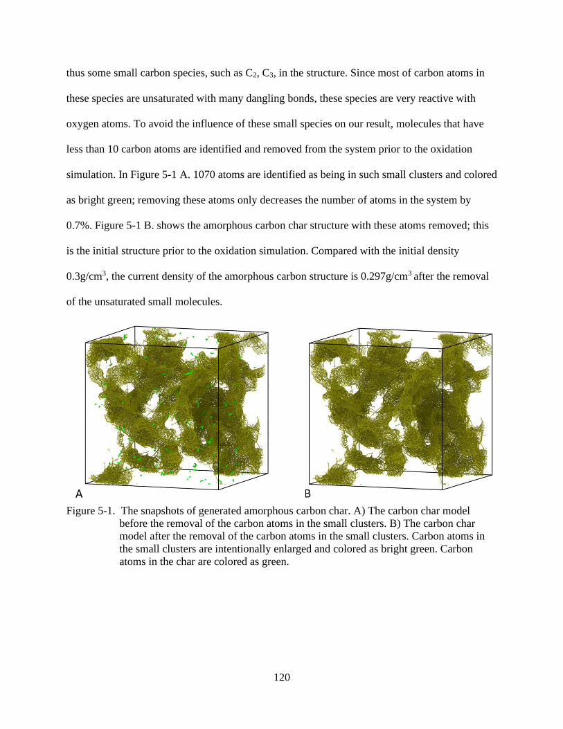
120

thus some small carbon species, such as C2, C3, in the structure. Since most of carbon atoms in

these species are unsaturated with many dangling bonds, these species are very reactive with

oxygen atoms. To avoid the influence of these small species on our result, molecules that have

less than 10 carbon atoms are identified and removed from the system prior to the oxidation

simulation. In Figure 5-1 A. 1070 atoms are identified as being in such small clusters and colored

as bright green; removing these atoms only decreases the number of atoms in the system by

0.7%. Figure 5-1 B. shows the amorphous carbon char structure with these atoms removed; this

is the initial structure prior to the oxidation simulation. Compared with the initial density

0.3g/cm3, the current density of the amorphous carbon structure is 0.297g/cm3 after the removal

of the unsaturated small molecules.

Figure 5-1. The snapshots of generated amorphous carbon char. A) The carbon char model

before the removal of the carbon atoms in the small clusters. B) The carbon char

model after the removal of the carbon atoms in the small clusters. Carbon atoms in

the small clusters are intentionally enlarged and colored as bright green. Carbon

atoms in the char are colored as green.

121

5.2.3 Overall Simulation Settings

The LAMMPS software[53] is used for all microstructure generation and oxidation

simulations presented in this work. During the relaxation of the initial structure and bond

formation process (steps 1-3) of the generation of CF, the computationally efficient Dreiding

force field[24] is employed to describe the covalent atomic interactions, while the Lennard Jones

(LJ) potential is employed to describe the van der Waals interactions. The Moltemplate

package[101] is used to attach the Dreiding force field and bonding information to the

coordination files. In step 5 of the generation of the CF model and in all subsequent steps and the

oxidation simulations, the more physically realistic ReaxFF (reactive force field)[104] is used;

this force field has been successfully used to model various novel carbon-like structures,

including graphene[165] and carbon nanotubes[113]. Moreover, ReaxFF allows dynamic bond

breakage and formation by using the concept of the bond order within a reactive system.

The Ovito software[21] and its Python interface are used to visualize the simulations and

to analyze the results of the oxidation simulation. The Packmol package[100] is used for

insertion of structural units in the CF generation process and insertion of oxygen atoms in the

oxidation models. In order to make the oxidation of the CF and char simulation comparable, the

initial concentration of oxygen atom is set to 0.5 mol/L in both models. It should be noted that to

increase the chance of reaction and accelerate the oxidation simulation process, the oxygen

concentration in this work is much higher than in the atmosphere and mesosphere. Since, as we

shall see, the oxidation process primarily involves the oxidation of single carbon atoms to form

CO, this high pressure does not introduce chemical reactions not present at low pressures; it

merely, increases the reaction rate without changing the overall kinetics. The “Construct Surface

Mesh” capability in Ovito is used to construct the polyhedral surface mesh around carbon atoms

122

for analysis. Although the shape is irregular, the actual occupied volume of generated CF and

char models can be accurately obtained from the enclosed area using this method. Figure 5-2 A.

and B. show the generated CF and amorphous char models with the surface meshes colored as

translucent red. To initialize the oxidation simulations, 7893 (for CF) and 2548 (for char) oxygen

atoms are packed to in the empty space of the simulation cell, as shown in Figure 5-2 C. and D.

Since the ReaxFF potential uses bond order to determine if two atoms are bond with each other,

the minimal distance tolerance between one oxygen atom and the other atoms is set to 2 Å to

avoid unnecessary bond formation during the packing process and energy minimization. After

oxygen atoms insertion, the oxidation of CF and amorphous char systems are simulated by the

following steps: (1) Relax the initial system by energy minimization with the conjugate gradient

algorithm, (2) equilibrate the system at the zero pressure and at 300K for 10ps, and (3) rescale

the temperature to the target temperature 𝑇 with the canonical ensemble (NVT) for 90 ps to

simulate the initial stage of the oxidation process. To investigate the influence of the temperature

on the oxidation process, the target temperature 𝑇 in each simulation is set to a temperature

between 1000 K to 4000 K in 500 K intervals. Moreover, we find that the simulation cell of CF

model slightly shrinks after equilibration in the steps 1 and 2, slightly increasing the initial

oxygen concentration in the CF simulation to 0.53 mol/L. In addition, although the simulation

cell of the amorphous carbon char doesn’t shrink during the equilibration, we observe that many

oxygen atoms are adsorbed onto the surface of the amorphous char due to the large surface area.

Therefore, the initial free oxygen concentration in the amorphous carbon char model decreases to

0.46 mol/L after equilibration. Periodic boundary conditions are applied, and the time step is 0.1

fs in the oxidation simulation. The analysis of the species is performed with a 1.8 Å cutoff for all

atom pairs to determine if bond forms between atoms. The molecular species present are

123

inventoried every 10 fs. These data provide detailed information for the analysis of the initial

stage of the oxidation.

Figure 5-2. The snapshots of fiber and char models after oxygen insertion. A) 3D view of the

generated CF model with the surface mesh. The simulation cell is hidden for a better

view. B) 3D view of the generated amorphous carbon char model with the surface

mesh. C-D) The oxidation models of CF and amorphous carbon char after oxygen

atoms insertion. The carbon atoms are colored as green. The surface mesh area is

colored as translucent bright green in A-B. Oxygen atoms are colored as red in C-D.

5.2.4 Reaction Parameter Analysis

The dynamic snapshots of MD simulation contain detailed information of the trajectory

of all atoms. Therefore, every atom that makes up each molecule can be tracked. By tracing the

path of each atom through its various bonding environments, the lifetime of each species can be

124

identified and counted separately. Since the true lifetime of any gaseous species that is present at

the end of the simulation cannot be determined, they are not considered in the lifetime

calculations.

The CF-oxygen and char-oxygen reaction mechanism is fairly complicated. It is beyond

the scope of this paper to take account all the factors that influence the initial stage of oxidation

of CF and char. A necessary and sufficient oxidation mechanism is described here based on

Schwartzentruber’s model[156], where he uses finite-rate gas–surface reaction models to predict

macroscopic behavior of CF oxidation such as mass loss rates and rate parameters. As shown in

Table 5-1, we consider several possible reaction mechanisms and analyze six oxidation models.

The complexity of each model is determined by the number of specific chemical reactions that

are included in the analysis. In all of these models, we assume that all reactions are first order

elementary reactions and that the rate is only related to the instantaneous concentration of

reactants. Based on Schwartzentruber’s model and our findings in Section 5.2.5, oxygen atoms

can be adsorbed and desorbed on the empty sites of the surface of CF and carbon char. Reactions

1 and 2 in Table 1 account for the reversible oxygen adsorption/desorption mechanism, where

(s), O and Os are an empty site on the carbon matrix, atomic oxygen and surface-adsorbed

oxygen atoms respectively. Reactions 3 and 4 describe the reaction of carbon atoms in CF/char

with the atomic and adsorbed oxygen atom to generate CO respectively. Although the initial

large separation of atomic oxygen atoms means that there is little formation of oxygen molecules

during the equilibration, it is possible for oxygen molecules to be generated during the oxidation

simulation at high temperature. This mechanism is described in reaction 5. Reaction 6 is the

dissociative adsorption of the 𝑂2, where one of the O atoms from the O2 molecules adsorbs on an

empty carbon site. Reaction 7 describes the possible dissociative adsorption of CO2, where one

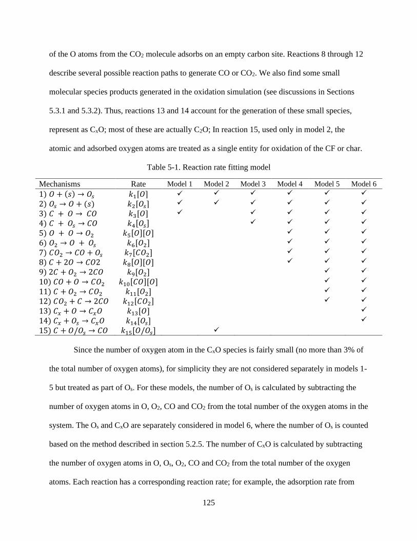
125

of the O atoms from the CO2 molecule adsorbs on an empty carbon site. Reactions 8 through 12

describe several possible reaction paths to generate CO or CO2. We also find some small

molecular species products generated in the oxidation simulation (see discussions in Sections

5.3.1 and 5.3.2). Thus, reactions 13 and 14 account for the generation of these small species,

represent as CxO; most of these are actually C2O; In reaction 15, used only in model 2, the

atomic and adsorbed oxygen atoms are treated as a single entity for oxidation of the CF or char.

Table 5-1. Reaction rate fitting model

Mechanisms Rate Model 1 Model 2 Model 3 Model 4 Model 5 Model 6

1) 𝑂 + (𝑠) → 𝑂𝑠 𝑘1[𝑂] ✓ ✓ ✓ ✓ ✓ ✓

2) 𝑂𝑠 → 𝑂 + (𝑠) 𝑘2[𝑂𝑠] ✓ ✓ ✓ ✓ ✓ ✓

3) 𝐶 + 𝑂 → 𝐶𝑂 𝑘3[𝑂] ✓ ✓ ✓ ✓ ✓

4) 𝐶 + 𝑂𝑠 → 𝐶𝑂 𝑘4[𝑂𝑠] ✓ ✓ ✓ ✓

5) 𝑂 + 𝑂 → 𝑂2 𝑘5[𝑂][𝑂] ✓ ✓ ✓

6) 𝑂2 → 𝑂 + 𝑂𝑠 𝑘6[𝑂2] ✓ ✓ ✓

7) 𝐶𝑂2 → 𝐶𝑂 + 𝑂𝑠 𝑘7[𝐶𝑂2] ✓ ✓ ✓

8) 𝐶 + 2𝑂 → 𝐶𝑂2 𝑘8[𝑂][𝑂] ✓ ✓ ✓

9) 2𝐶 + 𝑂2 → 2𝐶𝑂 𝑘9[𝑂2] ✓ ✓

10) 𝐶𝑂 + 𝑂 → 𝐶𝑂2 𝑘10[𝐶𝑂][𝑂] ✓ ✓

11) 𝐶 + 𝑂2 → 𝐶𝑂2 𝑘11[𝑂2] ✓ ✓

12) 𝐶𝑂2 + 𝐶 → 2𝐶𝑂 𝑘12[𝐶𝑂2] ✓ ✓

13) 𝐶𝑥 + 𝑂 → 𝐶𝑥𝑂 𝑘13[𝑂] ✓

14) 𝐶𝑥 + 𝑂𝑠 → 𝐶𝑥𝑂 𝑘14[𝑂𝑠] ✓

15) 𝐶 + 𝑂/𝑂𝑠 → 𝐶𝑂 𝑘15[𝑂/𝑂𝑠] ✓

Since the number of oxygen atom in the CxO species is fairly small (no more than 3% of

the total number of oxygen atoms), for simplicity they are not considered separately in models 1-

5 but treated as part of Os. For these models, the number of Os is calculated by subtracting the

number of oxygen atoms in O, O2, CO and CO2 from the total number of the oxygen atoms in the

system. The Os and CxO are separately considered in model 6, where the number of Os is counted

based on the method described in section 5.2.5. The number of CxO is calculated by subtracting

the number of oxygen atoms in O, Os, O2, CO and CO2 from the total number of the oxygen

atoms. Each reaction has a corresponding reaction rate; for example, the adsorption rate from

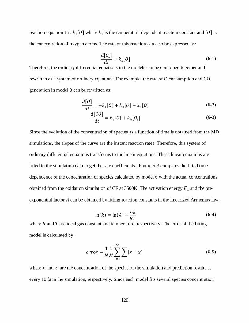
126

reaction equation 1 is 𝑘1[𝑂] where 𝑘1 is the temperature-dependent reaction constant and [𝑂] is

the concentration of oxygen atoms. The rate of this reaction can also be expressed as:

𝑑[𝑂𝑠]

𝑑𝑡= 𝑘1[𝑂] (6-1)

Therefore, the ordinary differential equations in the models can be combined together and

rewritten as a system of ordinary equations. For example, the rate of O consumption and CO

generation in model 3 can be rewritten as:

𝑑[𝑂]

𝑑𝑡= −𝑘1[𝑂] + 𝑘2[𝑂] − 𝑘3[𝑂] (6-2)

𝑑[𝐶𝑂]

𝑑𝑡= 𝑘3[𝑂] + 𝑘4[𝑂𝑠] (6-3)

Since the evolution of the concentration of species as a function of time is obtained from the MD

simulations, the slopes of the curve are the instant reaction rates. Therefore, this system of

ordinary differential equations transforms to the linear equations. These linear equations are

fitted to the simulation data to get the rate coefficients. Figure 5-3 compares the fitted time

dependence of the concentration of species calculated by model 6 with the actual concentrations

obtained from the oxidation simulation of CF at 3500K. The activation energy 𝐸𝑎 and the pre-

exponential factor 𝐴 can be obtained by fitting reaction constants in the linearized Arrhenius law:

ln(𝑘) = ln(𝐴) −𝐸𝑎

𝑅𝑇 (6-4)

where 𝑅 and 𝑇 are ideal gas constant and temperature, respectively. The error of the fitting

model is calculated by:

𝑒𝑟𝑟𝑜𝑟 =1

𝑁

1

𝑀∑ ∑|𝑥 − 𝑥′|

𝑀

𝑖=1

(6-5)

where 𝑥 and 𝑥′ are the concentration of the species of the simulation and prediction results at

every 10 fs in the simulation, respectively. Since each model fits several species concentration

127

curves as the function of time for different temperatures, the error is averaged by the number of

the fitting curves 𝑀 and the number of the simulations at various temperatures 𝑁. The error

analysis and comparison between models will be discussed in Section 5.3.

Figure 5-3. The predictive curve of species fitted to model 6 (red curves) and the data obtained

from the MD simulation (blue curve) from the oxidation simulation of CF under

3500K.

5.2.5 Oxygen Adsorption on Surface

During the oxidation, the main products observed are CO, O2 and CO2. Therefore, the

primary processes of interest are the formation of CO, O2 and CO2 from the initial atomic

oxygen atmosphere. As shown in the Figure 5-4(a), the fraction of initial oxygen atoms in four

main gaseous species (𝑁𝑂 + 𝑁𝐶𝑂 + 2𝑁𝑂2+ 2𝑁𝐶𝑂2

)/𝑁𝑡𝑜𝑡𝑎𝑙 is not conserved during the whole

initial stage of the oxidation, where 𝑁𝑡𝑜𝑡𝑎𝑙 is the total number of oxygen atoms in the system.

However, since the total number of oxygen atoms 𝑁𝑡𝑜𝑡𝑎𝑙 in the simulation is fixed, this indicates

that additional processes are also taking place. We observed that almost all of the uncounted

128

oxygen atoms are adsorbed on the surface of the carbon fiber, as evidenced by Figure 5-4(c-d).

And the total number of oxygen atoms 𝑁𝑡𝑜𝑡𝑎𝑙 can be refined as following:

𝑁𝑡𝑜𝑡𝑎𝑙 = 𝑁𝑂 + 𝑁𝐶𝑂 + 2𝑁𝑂2+ 2𝑁𝐶𝑂2

+ 𝑁𝑂(𝑠) + 𝑁𝐶𝑥𝑂 (6-6)

where 𝑁𝑂, 𝑁𝐶𝑂, 𝑁𝑂2, 𝑁𝐶𝑂2

, 𝑁𝑂(𝑠) and 𝑁𝐶𝑥𝑂 are the number of O, CO, O2, CO2, Os and CxO,

respectively. Because the carbon fiber is composed of many independent graphitic sheets, each

sheet can be identified as an independent molecule Cm in the simulation, where m is the number

of carbon atoms in the sheet. The graphene sheets that adsorb oxygen atoms are identified as the

𝐶𝑚𝑂𝑛where n is the number of oxygen atoms in the molecule. Compared with the small

chemical species 𝐶𝑚′ 𝑂𝑛

′ , graphene sheet has a very large value for 𝑚 and a small value 𝑛.

Therefore, the molecule 𝐶𝑚𝑂𝑛 is identified as the graphene sheet with oxygen adsorption where

𝑚 − 𝑛 > 100 and oxygen atoms in this kind of 𝐶𝑚𝑂𝑛 are identified as atoms adsorbed on carbon

surface. It should be noted that the threshold value 100 that determines whether the molecule is

graphene sheet or other kind of species is somewhat arbitrary. We identified this value as

suitable work by trying the different values and comparing the filtered results. As shown in

Figure 5-4 B., after considering oxygen atom adsorption, the number of oxygen atoms accounted

for by the four gaseous species and on the surface of fiber is more than 97% of the total number

of oxygen atoms in the simulation at all temperatures. Moreover, we found that main species in

the left unaccounted molecules CxO is C2O with a very short lifetime due to the high reactivity.

A detailed discussion about the lifetime of C2O and other species will be presented in section

5.3.1. Figure 5-4 C-D. and Figure 5-4 E-F. show the direct evidence that oxygen atoms adsorbed

on the surface of the fiber and amorphous carbon at different simulation time, respectively. The

small molecules are intentionally hidden and only graphene sheets or amorphous carbon meeting

the above requirement are shown in these figures. Although the minimum distance between one

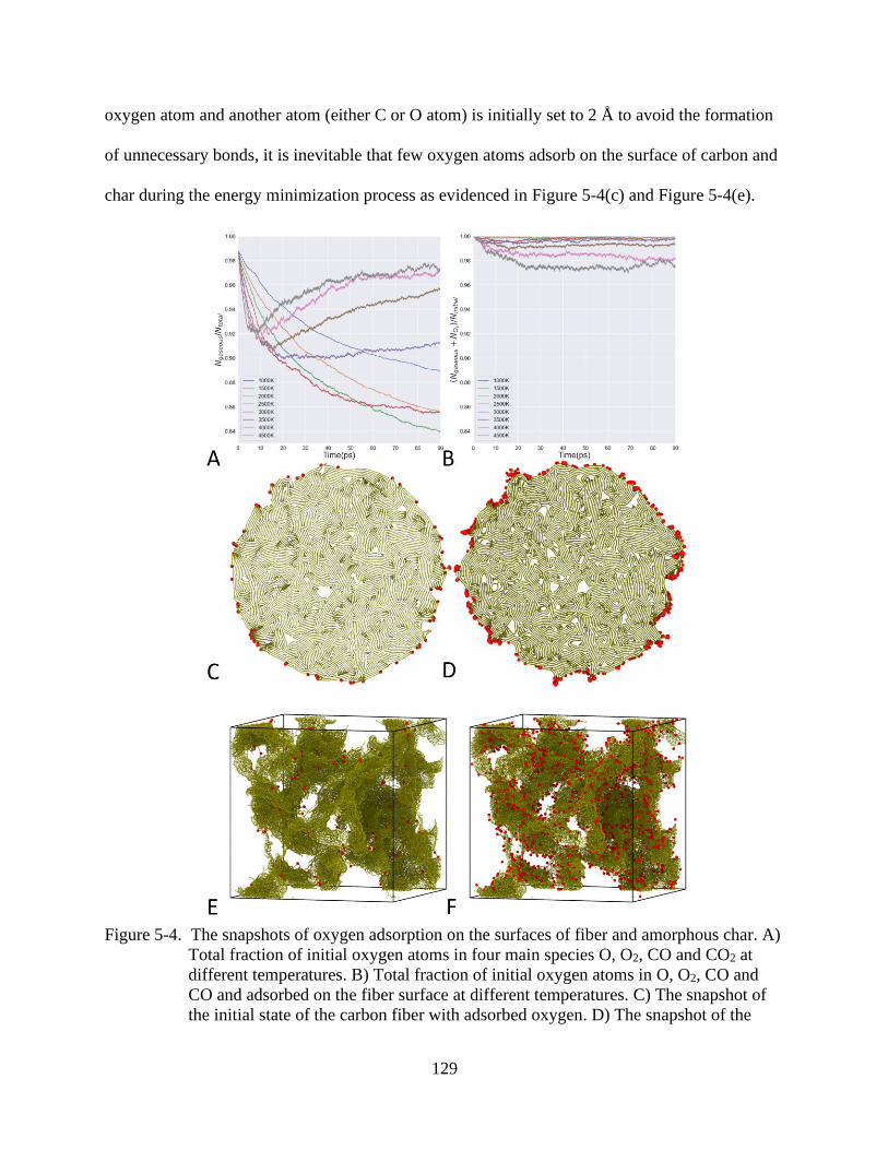
129

oxygen atom and another atom (either C or O atom) is initially set to 2 Å to avoid the formation

of unnecessary bonds, it is inevitable that few oxygen atoms adsorb on the surface of carbon and

char during the energy minimization process as evidenced in Figure 5-4(c) and Figure 5-4(e).

Figure 5-4. The snapshots of oxygen adsorption on the surfaces of fiber and amorphous char. A)

Total fraction of initial oxygen atoms in four main species O, O2, CO and CO2 at

different temperatures. B) Total fraction of initial oxygen atoms in O, O2, CO and

CO and adsorbed on the fiber surface at different temperatures. C) The snapshot of

the initial state of the carbon fiber with adsorbed oxygen. D) The snapshot of the

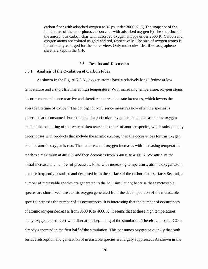
130

carbon fiber with adsorbed oxygen at 30 ps under 2000 K. E) The snapshot of the

initial state of the amorphous carbon char with adsorbed oxygen F) The snapshot of

the amorphous carbon char with adsorbed oxygen at 30ps under 2500 K. Carbon and

oxygen atoms are colored as gold and red, respectively. The size of oxygen atoms is

intentionally enlarged for the better view. Only molecules identified as graphene

sheet are kept in the C-F.

5.3 Results and Discussion

5.3.1 Analysis of the Oxidation of Carbon Fiber

As shown in the Figure 5-5 A., oxygen atoms have a relatively long lifetime at low

temperature and a short lifetime at high temperature. With increasing temperature, oxygen atoms

become more and more reactive and therefore the reaction rate increases, which lowers the

average lifetime of oxygen. The concept of occurrence measures how often the species is

generated and consumed. For example, if a particular oxygen atom appears as atomic oxygen

atom at the beginning of the system, then reacts to be part of another species, which subsequently

decomposes with products that include the atomic oxygen, then the occurrences for this oxygen

atom as atomic oxygen is two. The occurrence of oxygen increases with increasing temperature,

reaches a maximum at 4000 K and then decreases from 3500 K to 4500 K. We attribute the

initial increase to a number of processes. First, with increasing temperature, atomic oxygen atom

is more frequently adsorbed and desorbed from the surface of the carbon fiber surface. Second, a

number of metastable species are generated in the MD simulation; because these metastable

species are short lived, the atomic oxygen generated from the decomposition of the metastable

species increases the number of its occurrences. It is interesting that the number of occurrences

of atomic oxygen decreases from 3500 K to 4000 K. It seems that at these high temperatures

many oxygen atoms react with fiber at the beginning of the simulation. Therefore, most of CO is

already generated in the first half of the simulation. This consumes oxygen so quickly that both

surface adsorption and generation of metastable species are largely suppressed. As shown in the

131

Figure 5-5 B., the average lifetime of O2 is fairly short compared with that of the atomic oxygen.

However, unlike O, the average lifetime of O2 increases with the increase of temperature. The

number of occurrences for oxygen molecules also increases from 1000 K to 2500 K and then

decreases from 3000 K to 4500 K. The initial increase is due to the formation of molecules from

the highly reactive atomic oxygen; the decrease is due to the rapid generation of CO at high

temperature which decreases the possibility of formation of O2 since most of O are consumed for

CO formation. The lifetime of CO is long compared with other species (seeing Figure 5-5 C.)

and largely independent of temperature. The occurrence of CO increases with the increase of

temperature indicating that more CO involved with the reaction. As we discussed in section

5.2.5, the oxygen atoms in the four main gaseous species O, CO, O2, CO2 and adsorbed oxygens

Os account for more than 97% of the total oxygen atoms, the remaining 3% oxygen atoms mainly

are in small molecules, mainly in the dicarbon monoxide (C2O) molecules, which is extremely

reactive and short lived. Indeed, as shown in Figure 5-5 D. and E., the lifetime of CO2 and C2O

less than 3 ps, indicative of its highly reactivity. This short lifetime of C2O may be one reason

that it not observed in the experiment. The occurrence of C2O increases with increasing

temperature, indicating that this molecule is frequently generated and then decomposes at high

temperature. Figure 5-5 F. shows the average lifetime of Os decreases with the increasing

temperature from 2000 K to 4500 K, indicating increasing reactivity. Also, the increase of

number of occurrences of Os with increasing temperature shows that oxygen atoms are easier

adsorbed on the fiber surface at high temperature but also quickly desorbed.

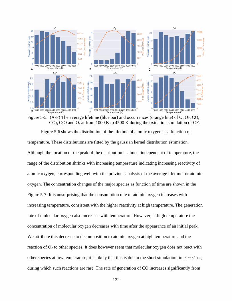
132

Figure 5-5. (A-F) The average lifetime (blue bar) and occurrences (orange line) of O, O2, CO,

CO2, C2O and Os at from 1000 K to 4500 K during the oxidation simulation of CF.

Figure 5-6 shows the distribution of the lifetime of atomic oxygen as a function of

temperature. These distributions are fitted by the gaussian kernel distribution estimation.

Although the location of the peak of the distribution is almost independent of temperature, the

range of the distribution shrinks with increasing temperature indicating increasing reactivity of

atomic oxygen, corresponding well with the previous analysis of the average lifetime for atomic

oxygen. The concentration changes of the major species as function of time are shown in the

Figure 5-7. It is unsurprising that the consumption rate of atomic oxygen increases with

increasing temperature, consistent with the higher reactivity at high temperature. The generation

rate of molecular oxygen also increases with temperature. However, at high temperature the

concentration of molecular oxygen decreases with time after the appearance of an initial peak.

We attribute this decrease to decomposition to atomic oxygen at high temperature and the

reaction of O2 to other species. It does however seem that molecular oxygen does not react with

other species at low temperature; it is likely that this is due to the short simulation time, ~0.1 ns,

during which such reactions are rare. The rate of generation of CO increases significantly from

133

1000 K to 4500 K. The concentration of CO at 4500 K saturates with time because the oxidation

process is now complete with essentially all of the initial oxygen having reacted to CO: there is

little O2, CO2, Os and CxO remaining. It is likely that if the simulations at lower temperature

were run for longer, they would also finally reach completion; indeed the 3500 K and 4000 K

simulations are both approaching complete reaction of O to CO. Similar to O2, the concentration

of CO2 at high temperature increases initially and then decreases indicating the decomposition

from CO2 to O and CO, which corresponds well with the analysis of average lifetime of CO2. As

shown in Figure 5-7, the concentration of Os also increases at first and then decreases. At low

temperature, the number of Os increases showing that oxygen atom tends to adsorb on the fiber

surface and not be reactive, which is also indicated by the nearly constant number of Os + O as

function of time; we discuss the long-time evolution below. At high temperature, Os is initially

adsorbed on the surface then reacts with other atoms or desorbs from the fiber surface, both of

which can lead to the decrease of the number of Os after the peak. The total number of Os + O

atoms decreases with increasing temperature, showing that oxygen atom tends to react with other

atoms and transform to other molecules at high temperature. Another interesting aspect is that

the highest concentrations of these intermediate molecules are not at the highest temperature; the

peaks of concentration for O2, CO2 and Os are 3500 K, 3000 K and 2000 K, respectively.

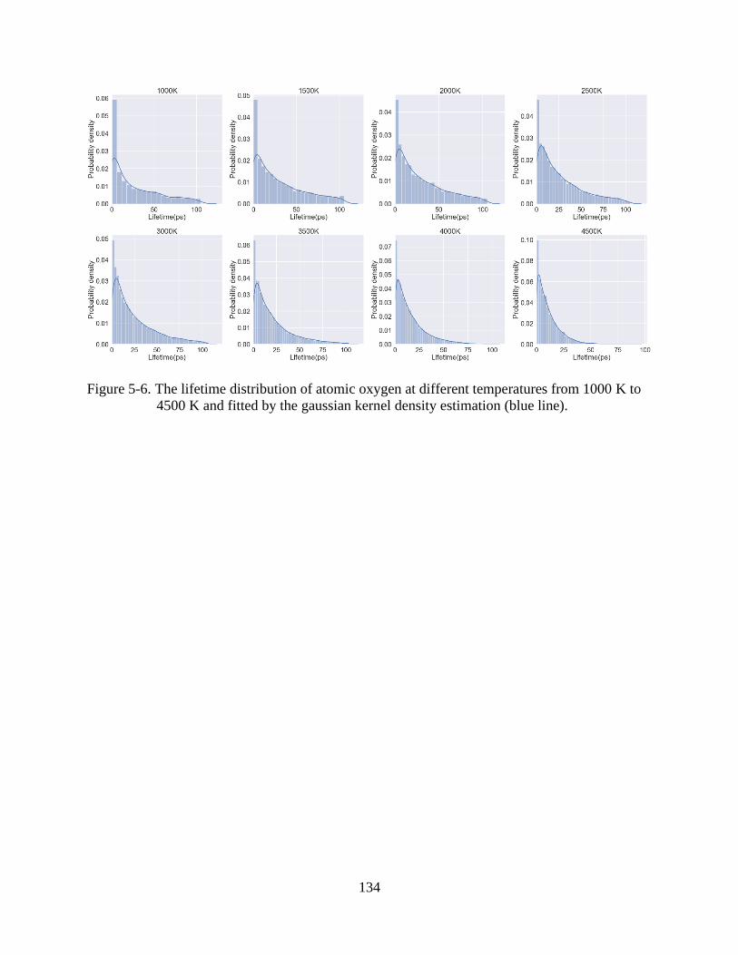
134

Figure 5-6. The lifetime distribution of atomic oxygen at different temperatures from 1000 K to

4500 K and fitted by the gaussian kernel density estimation (blue line).

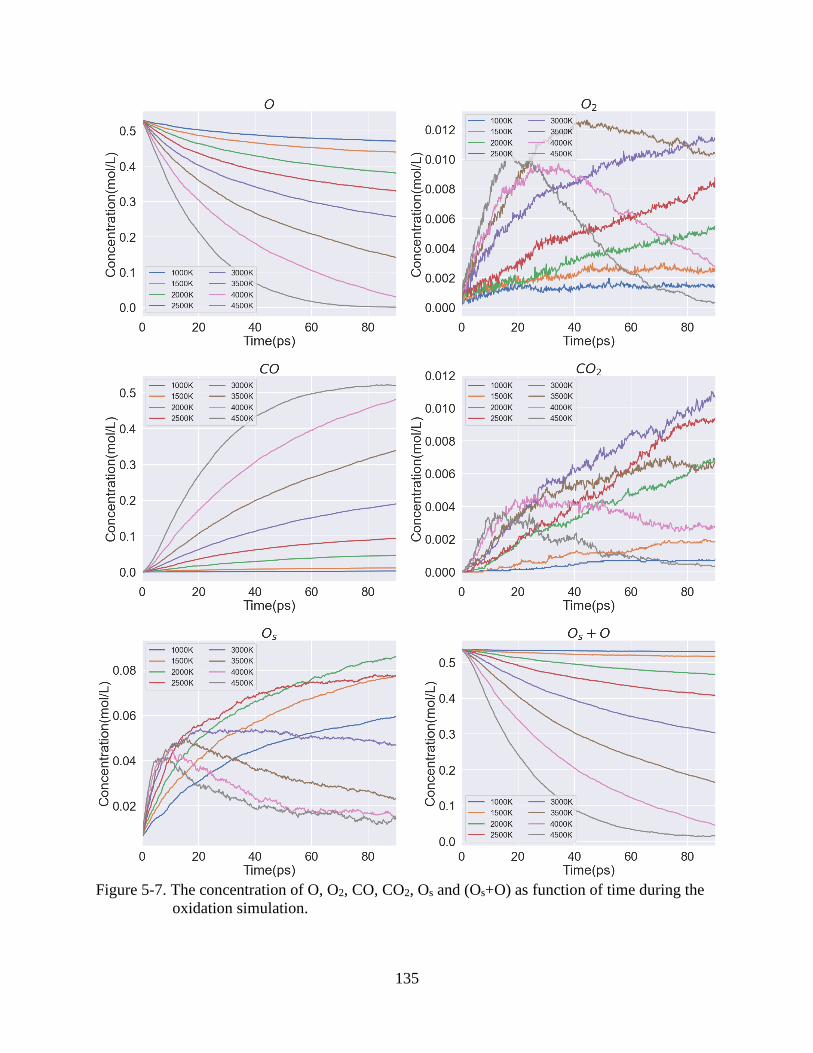
135

Figure 5-7. The concentration of O, O2, CO, CO2, Os and (Os+O) as function of time during the

oxidation simulation.

136

By fitting the six models, we obtain the reaction constants of each reaction equations at

different temperatures. By fitting the reaction constants at different temperatures, we find that the

computed reaction constants for all of the species that have substantial concentrations follow the

Arrhenius equation, as excepted. For species with very low concentrations, the data is too noisy

to perform a quantitative analysis. The reactions for which Arrhenius fits can be made, yield

estimates of the activation energy that are consistent among the various models, as shown in

Figure 5-8. It should be noted that the reaction rates at 4500 K are not included for Model 1, 2

and 4 because of the unideal fitting. We found that the three important reactions (a) 𝑂 + (𝑠) →

𝑂𝑠 (b) 𝐶 + 𝑂 → 𝐶𝑂 , and (c) 𝑂 + 𝑂 → 𝑂2 follow the Arrhenius equation. The activation energies

with the error bars for the three reactions are listed in Table 5-2. The activation energy for

oxygen adsorption is similar with that for the oxygen molecule generation and the activation

energy for carbon oxidation is around 57 kJ/mol. In addition, the error of each model, as defined

by Eq. 6-5, is shown in Table 5-2. Since Models 1-3 include largely the same reaction equations,

it is not surprising that they have similar errors. Compared with Models 1-3, Models 4-6 have

smaller errors due to the larger number of fitting parameters in the system of reaction equations.

It is interesting that adding more reaction equations in the model does not lead to a better fit

result and less error. Compared with the 12 reactions in Model 5, Model 4 uses 8 reactions to

describe the processes, and yet has a smaller error. Since Model 4 has the least error of Models

1-5, which don’t consider CxO, we use this model to predict the species change in a longer timer

scale up to 500 ps (see Figure 5-9). As is expected, the O is consumed much faster at high

temperature than at low temperature. In addition, almost all O transform to CO at 3500 K and

4000 K. For the rest of temperatures, the concentration of CO still increases more time is needed

137

to completely deplete the O. Except at the low temperature 1000 K, the concentration of Os

increases first and then gradually decreases. The highest peak of Os occurs at 2000 K.

Figure 5-8. Logarithm of the reaction rate against the inverse temperature for different reactions

A) 𝑂 + (𝑠) → 𝑂𝑠 B) 𝐶 + 𝑂 → 𝐶𝑂 C) 𝑂 + 𝑂 → 𝑂2 for the oxidation of CF.

Table 5-2. The activation energy of reactions fitted from model 1 to model 6 and the prediction

error of each model for the oxidation of CFs.

𝑂 + (𝑠) → 𝑂𝑠 (𝑘𝐽/𝑚𝑜𝑙) 𝐶 + 𝑂 → 𝐶𝑂 (𝑘𝐽/𝑚𝑜𝑙) 𝑂 + 𝑂 → 𝑂2 (𝑘𝐽/𝑚𝑜𝑙) Error

Model 1 17.12±2.60 58.87±7.05 N/A 0.15

Model 2 22.88±3.83 N/A N/A 0.14

Model 3 22.03±3.52 54.94±4.55 N/A 0.15

Model 4 19.68±3.54 58.60±4.18 20.64±2.45 0.04

Model 5 19.48±2.99 58.41±4.91 23.48±2.77 0.05

Model 6 21.94±3.72 53.13±5.68 25.10±2.92 0.03

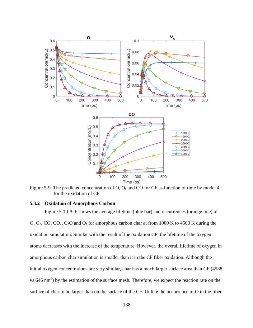
138

Figure 5-9. The predicted concentration of O, Os and CO for CF as function of time by model 4

for the oxidation of CF.

5.3.2 Oxidation of Amorphous Carbon

Figure 5-10 A-F shows the average lifetime (blue bar) and occurrences (orange line) of

O, O2, CO, CO2, C2O and Os for amorphous carbon char at from 1000 K to 4500 K during the

oxidation simulation. Similar with the result of the oxidation CF, the lifetime of the oxygen

atoms decreases with the increase of the temperature. However, the overall lifetime of oxygen in

amorphous carbon char simulation is smaller than it in the CF fiber oxidation. Although the

initial oxygen concentrations are very similar, char has a much larger surface area than CF (4588

vs 646 nm2) by the estimation of the surface mesh. Therefore, we expect the reaction rate on the

surface of char to be larger than on the surface of the CF. Unlike the occurrence of O in the fiber

139

oxidation, the occurrence of O remains in a similar level in the char oxidation. As shown in the

Figure 5-10 B., the average lifetime of O2 is also increases from 1000 K to 4000 K and then

decreases from 4000 K to 4500 K. Compared with CF oxidation simulation, O2 has a longer

lifetime and a much smaller occurrence in oxidation simulation. With the increase of the

temperature, the occurrence of CO increases in a similar manner as it does with the CF oxidation.

However, it is interesting that the lifetime of CO decreases from 1000 K to 2500K and increases

from 2500 K to 4500 K. It should be noted that the species counted in the lifetime calculation are

all consumed in the reactions and transformed to other species. We found that average lifetime of

CO that last at the end of the simulation is 56~72 ps at various temperature and the number is

much larger than the number of CO involved in the reactions. Therefore, most of CO are final

product. For the partial intermediate reactant CO, the best suitable reaction temperature is around

2500 K in the char oxidation simulation. At lower temperature, the reaction constant is too low

resulting in the higher lifetime. At higher temperature, the reaction that consumes CO need to

compete with other reactions which lowers the probability that CO react with other molecules

and increases the lifetime of CO. As shown in Figure 5-10 D. the lifetime of CO at the

temperature from 1000 K to 3500 K is fairly short and similar with the result in fiber simulation.

But unlike the fiber simulation, CO2 has a higher lifetime at 4000 and 4500 K. Moreover, the

occurrence of CO2 increases from 1000 K to 2000 K and decreases from 2000 K to 4500 K. The

peak indicates that the reactions that consume or produce CO2 mostly occur at 2000 K. Figure

5-10 E. shows the occurrence of C2O also increases from the 1000 to 4500K. Also, the average

lifetime of C2O in char oxidation is larger than it in CF oxidation. Figure 5-10 F. shows the

average lifetime of Os has its largest value, over 20 ps, at 2500 K. This lifetime value of Os in the

char simulation is larger than it in the CF simulation at the same temperature. Since the total

140

number of oxygen atoms in char oxidation is only about one-third of the number in the fiber

simulation, most of species undergo fewer reactions in the char oxidation than in the fiber

simulation at the same temperature. However, the occurrence of Os is higher in the char

simulation at low temperature because of its large surface area.

Figure 5-10. A-F) The average lifetime (blue bar) and occurrences (orange line) of O, O2, CO,

CO2, C2O and Os at from 1000 K to 4500 K during the oxidation simulation of

amorphous carbon char.

Figure 5-11 shows the change in the concentration of the major species as a function of

time in the amorphous carbon char oxidation. As in the case of the CF oxidation, the

consumption rate of atomic oxygen and the generation rate of CO increases with the increasing

temperature. However, due to the smaller system and larger surface area of char, the slope of O

and CO curves are steeper than these in CF oxidation indicating the higher reaction rate.

Moreover, the curves of O2 and CO2 are also similar with those in the CF simulation: they

increase with increasing temperature and then decrease at high temperature. Similar with the CF

oxidation, the curve of Os is also increase with temperature and then decreases, indicating similar

141

adsorption and desorption mechanisms. The total number of Os+O atoms decreases with time,

showing that atomic and adsorbed oxygen atoms react to form to other molecules. The Os+O

curve reaches almost zero at around 50ps in the char simulation at 4500 K. The completion time

of Os+O is shorter than it in CF simulation. In conclusion, the reaction mechanisms in the char

and fiber oxidation are similar. However, oxygen atoms tend to more readily adsorb on the

surface of char due to the larger surface area compared with carbon fiber.

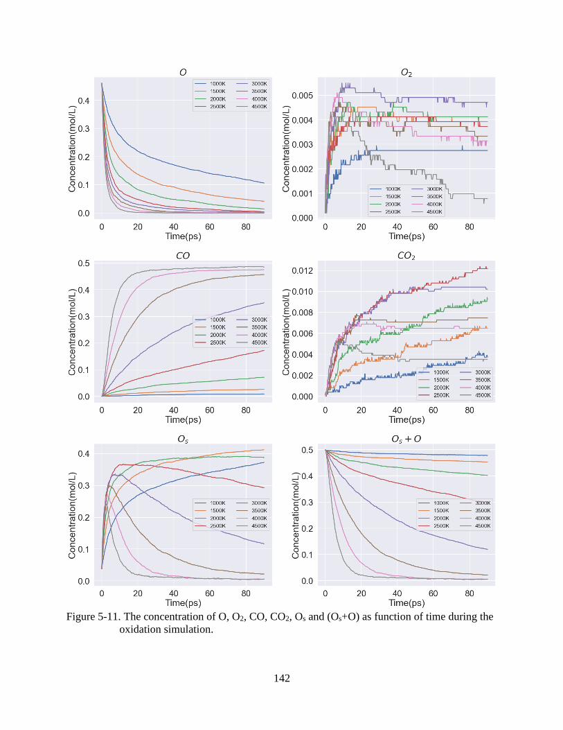
142

Figure 5-11. The concentration of O, O2, CO, CO2, Os and (Os+O) as function of time during the

oxidation simulation.

143

We use the same models to fit the oxidation curves for the oxidation of the amorphous

carbon char. Moreover, since the concentration of the O2 and CO2 is low in the amorphous

carbon char simulations, only O, CO and Os curves are used for fitting models. By fitting the

models 1-6, we find these models can get a good fitting for the temperature ranging from 2000 K

to 4500 K. Therefore, the unideal fitting results for simulations at 1000 K and 1500 K are

disregarded. We found only two reactions (a) 𝑂 + (𝑠) → 𝑂𝑠 (b) 𝐶 + 𝑂𝑠 → 𝐶𝑂 follow the

Arrhenius law (see Figure 5-12). The reason that the C + O reaction does not follow the

Arrhenius law is that, as shown in Figure 5-11, most oxygen atom are adsorbed on the surface of

char at the initial stage of the simulation. This leads the 𝐶 + 𝑂𝑠 → 𝐶𝑂 to be the dominant

reaction in the char oxidation. The activation energies of these two reactions and the fitting error

of models are listed in the Table 5-3. The average activation energy of 𝑂 + (𝑠) → 𝑂𝑠 among

model is 36kJ/mol which is larger than the value in the fiber oxidation. The average activation

energy of oxidation reaction 𝐶 + 𝑂𝑠 → 𝐶𝑂 is around 162 kJ/mol much larger than the activation

energy of 𝐶 + 𝑂 → 𝐶𝑂 in the fiber oxidation. Moreover, model 4 give relatively lower prediction

of the activation energy of the oxidation reaction around 137 kJ/mol. Since the oxygen is

adsorbed on the surface of char, desorption of CO from char surface also need to overcome the

energy barrier. That could contribute the higher oxidation energy in the char simulation.

Although the activation energy of reactions in char oxidation is higher, the pre-exponential factor

is also higher. Therefore, the reaction rate in the char oxidation is higher than the reaction rate in

the fiber oxidation. Model 4 also has the lowest fitting error among 6 models. Therefore, it is

also selected to predict the evolution of species up to 200 ps (see Figure 5-13). The trends of

prediction results are similar with the result of the oxidation of fiber. Also, the highest peak for

Os also occurs at 2000 K for the char oxidation simulations at the range from 2000 K to 4500K.

144

Figure 5-12. Logarithm of the reaction rate against the inverse temperature for different reactions

A) 𝑂 + (𝑠) → 𝑂𝑠 B) 𝐶 + 𝑂𝑠 → 𝐶𝑂 for the oxidation of amorphous carbon char.

Table 5-3. The activation energy of reactions fitted from model 1 to model 6 and the prediction

error of each model for the oxidation of amorphous carbon char.

𝑂 + (𝑠) → 𝑂𝑠 (𝑘𝐽/𝑚𝑜𝑙) 𝐶 + 𝑂𝑠 → 𝐶𝑂 (𝑘𝐽/𝑚𝑜𝑙) Error

Model 1 33.50±0.51 N/A 0.49

Model 2 31.32±1.32 N/A 0.21

Model 3 38.66±1.68 171.11±7.99 0.18

Model 4 32.13±2.33 137.00±14.00 0.05

Model 5 40.71±1.99 166.89±8.20 0.09

Model 6 40.56±2.14 174.66±7.34 0.07

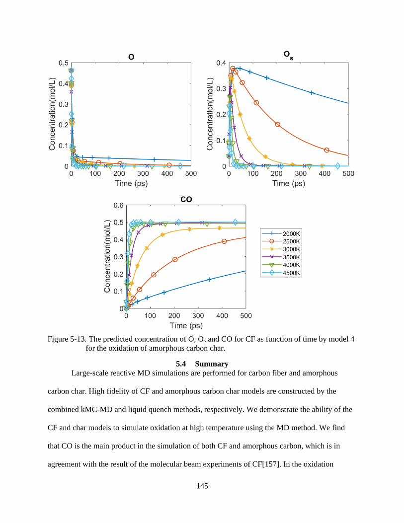
145

Figure 5-13. The predicted concentration of O, Os and CO for CF as function of time by model 4

for the oxidation of amorphous carbon char.

5.4 Summary

Large-scale reactive MD simulations are performed for carbon fiber and amorphous

carbon char. High fidelity of CF and amorphous carbon char models are constructed by the

combined kMC-MD and liquid quench methods, respectively. We demonstrate the ability of the

CF and char models to simulate oxidation at high temperature using the MD method. We find

that CO is the main product in the simulation of both CF and amorphous carbon, which is in

agreement with the result of the molecular beam experiments of CF[157]. In the oxidation

146

process, we found that atomic oxygen tends to adsorb on the surface of the carbon fiber and char.

Other species, most significantly O2, CO2 and CxO, are also found in the oxidation process but at

a much lower concentration than CO. The main species in the small molecules CxO is C2O,

which is highly reactive and has a short lifetime compared with other species. Six reaction

models are proposed. For CF oxidation simulation, the oxygen adsorption 𝑂 + (𝑠) → 𝑂𝑠, carbon

oxidation 𝐶 + 𝑂 → 𝐶𝑂 and oxygen formation 𝑂 + 𝑂 → 𝑂2 follows the Arrhenius law and have

activation energy 21 kJ/mol, 56 kJ/mol and 23 kJ/mol. For amorphous carbon oxidation

simulation, the oxygen adsorption 𝑂 + (𝑠) → 𝑂𝑠 and carbon oxidation 𝐶 + 𝑂 → 𝐶𝑂 follows the

Arrhenius law and have average activation energy 37 kJ/mol and 159 kJ/mol respectively.

Moreover, the longtime evolution of the concentration of each is also predicted for both CF and

amorphous char using the lowest error model.

Overall, we have demonstrated the great potential of these models for the simulation of

oxidation of carbon fiber and amorphous carbon. These models can provide insights into the

reaction mechanism that take place during the oxidation process. Because the oxidation process

is so complex, detailed analysis and advanced methods are needed in the post-processing of data.

For example, since the snapshot contains the trajectory of every atom, it is possible to separate

each individual reaction from the simulations. Then the rate of each reaction can be computed by

directly counting the number of individual reactions occurred in the simulation. Such an

approach was previously successfully applied in the analysis of hydrogen peroxide

decomposition[166]. However, unlike the hydrogen peroxide decomposition, separating

individual reactions in this work is substantially difficult since many individual reactions can

occur on the surface of CF/char at the same time.

147

CHAPTER 7

SUMMARY AND CONCLUSION

This dissertation has investigated the materials behavior under extreme conditions and

addressed three important problems. First, molecular dynamics is used to investigate mechanical

properties and deformation behavior of 𝛿- ZrH2 in the high-stress environment to increase the

understanding the dislocation mechanism, thereby helping the design of the next generation of

zirconium-based cladding. Second, the high-fidelity CF and amorphous carbon char models are

generated using kMC-MD and liquid quench method, respectively. Not only do the generation

methods make it possible to investigate more complicated CF/char-based composites, but also

the characterization of CF and amorphous char improves the understanding of the

microstructures, which can help to design the high-modulus carbon fiber. Last but not the least,

the oxidation process of CF and amorphous carbon char are simulated under high temperature

and the species evolution in the oxidation is studied.

In Chapter 3, the mechanical properties of ZrH2 are calculated and compared with the

DFT calculation results. We find the mechanical stability of ZrH2 is ensured by the COMB3

potential by meeting the stability conditions for cubic systems. The MD simulations of

nanoindentation are performed on the (100) and (110) planes to investigate the anisotropic

deformation behavior of ZrH2. By setting up the different initial conditions of simulation, such as

various indenter speeds and the thicknesses of the active layer, we find the speed of the indenter

doesn’t have a significant influence on the simulation results while the thickness of the active

layer does affect the behavior. The substrate effect becomes weaker with the increasing thickness

of active layer and the system size. Moreover, the force vs. indentation curve shows that

simulation results follow Hertz Law in the elastic region. The dimensionless load and hardness

agree well with the experimental results while the hardness calculated from the indentation is

148

overestimated by the COMB3 potential. The yield behavior is observed in the indentation

simulation on the (100) surface but not on the (110) surface. The phase change is also captured in

the simulation. The Zr atom sublattice changes from ABCABC (fcc) to hexagonal (ABAB) close

packing in the highly deformed region until the first load drop, while the H atom sublattice

remains simple cubic lattice due to the small atom size. The predominant dislocation identified in

the nanoindentation for both (100) and (110) surfaces are {100} <110> dislocations. Newly

nucleated dislocations parallel with the surface are observed for indentation on (100) surface and

the small dislocations are also observed for indentation on (110) surface with the indentation of

the indentation depth. In chapter 3, the factors that influence the deformation behavior have been

studied and the deformation mechanism of 𝛿-ZrH2 has been clarified.

In Chapter 4, the CF model is improved based on Desai’s kMC-MD model using the

ReaxFF force field. By combining the kinetic Monte Carlo method with large-scale MD, we

generate two types of CF models at a wide range of initial densities (from 1.2 g/cm3 to 2.0 g/cm3)

by controlling the CF shape with virtual force wall. These fiber core and thin fiber models

represent a small section of the interior region of large fiber and a very thin carbon fiber with a

well-defined surface, respectively. The generated fiber core models can have a large range of

final density from 1.45g-2.10 g/cm3 depending on the initial packing density. While the final

density of the thin fiber is independent of the initial packing density since free surface annihilate

most of pores. By extensively characterizing the structure features of the CF including the pore

size distribution, XRD analysis and hybridization state, the fidelity of both fiber core and thin

fiber models is ensured. In addition, the mechanical properties of CF are investigated by tensile

simulations. Discontinuous CF models are proposed by removing lines of carbon atoms at

random position in each graphene sheet to mimic the effect of the defects in the real CF along the

149

longitudinal direction, which reduces the tensile modulus to levels comparable to real CF.

Moreover, the axial tensile moduli of continuous and discontinuous fiber core model are in the

range of 0.2-5 GPa which is in good agreement with the experimental value for PAN and pitch-

based CFs. Compared with using graphite or carbon nanotube to model CF, the high-fidelity CF

model proposed in this work provides a better choice for simulation scientists to investigate the

properties of CF. Moreover, the proposed thin fiber model with the well-defined surface serves a

good foundation for modeling carbon-based composites or gas chemistry on CF surface.

In Chapter 5, amorphous carbon structures with a wide range of densities from 0.5g/cm3

to 3.2g/cm3 are generated using REBO and ReaxFF potentials by a liquid quench method. The

structural features of amorphous carbon structures are characterized by analyzing the

hybridization, pair correlation function, bond-angle distribution, and ring-size distribution. By

controlling the number of atoms and the volume of simulation cell, the liquid quench method is

able to generate amorphous structures from low density 0.5g/cm3, which is typical of

mesoporous char-like carbon to high density 3.2g/cm3, which is similar to nonporous dense

stacked graphene-sheet-like carbon. The characterization results show the generated carbon

structures by ReaxFF and REBO potentials have similar structural features from 0.5-2.5g/cm3.

By comparing Ranganathan’s result, ReaxFF tends to generate diamond-like carbon while REBO

tends to generate dense stacked graphene-sheet-like carbon.

In Chapter 6, oxidation simulation under high temperature from 1000K-4500K are

performed for CF and amorphous carbon using large-scale reactive molecular dynamics. We first

demonstrate that the CF and char models, which are generated by the methods described in

Chapters 4 and 5, have the ability to simulate oxidation process at various temperatures. CO is

found as the main product during the oxidation simulation for both CF and amorphous carbon

150

char, which matches well with the findings in Minton’s molecular beam experiment.[167] A

number of oxygen atoms are found to be adsorbed on the surface of CF and amorphous carbon

char. The average lifetime and lifetime distribution of O, CO, and other species, particularly O2,

CO2, CxO, are analyzed. By analyzing the evolution of the concentrations of the major species as

the function of time, the oxidation reaction mechanisms are investigated. Moreover, by fitting the

simulation results into six reaction models, we find several key reactions follow the Arrhenius

law and have similar activation energies among different models. In addition, the curves of

species change as function of time are predicted by the least-error model for CF and amorphous

carbon char. These models can provide goods insight on reactions mechanism in the oxidation

process during the ablation.

The plastic deformation behavior investigated in this dissertation gives us insights into

how dislocation structures grow under nanoindentation in a high-stress environment. Moreover,

this dissertation proposes an approach for modeling carbon-based amorphous microstructures

including CF and mesoporous char, and such approaches can be embedded into more

complicated models by combining with other metal or polymer systems. Our findings in the

oxidation simulation of CF and amorphous char elucidate the powerful application and potential

of these models for investigating structural properties of materials and non-equilibrium reactions

in the chemically aggressive environments which is difficult for experiments. The research

findings in this dissertation show that how models and simulations help research people

strengthen the understanding of the materials response under extreme conditions. Moreover,

these findings can be transferred to the mesoscale models, such as phase field model, served as

part of key parameters for a better prediction of the pyrolysis behavior of PICA.

151

LIST OF REFERENCES

[1] J. Wadsworth, G.W. Crabtree, R.J. Hemley, R. Falcone, I. Robertson, J. Stringer, P.

Tortorelli, G.T. Gray, M. Nicol, J. Lehr, S.W. Tozer, T. Fitzsimmons, J.S. Vetrano, C.L.

Ashton, S. Kitts, C. Landson, B. Campbell, G. Gruzalski, D. Stevens, Basic Research

Needs for Materials Under Extreme Environments. Report of the Basic Energy Sciences

Workshop on Materials Under Extreme Environments, June 11-13, 2007, Am. J. Nurs.

108 (2008) 24. http://www.osti.gov/servlets/purl/935440-WvJmE8/.

[2] C.E. Leiserson, N.C. Thompson, J.S. Emer, B.C. Kuszmaul, B.W. Lampson, D. Sanchez,

T.B. Schardl, There’s plenty of room at the top: What will drive computer performance

after Moore’s law?, Science (80-. ). 368 (2020). https://doi.org/10.1126/science.aam9744.

[3] G. Makov, C. Gattinoni, A. De Vita, Ab initio based multiscale modelling for materials

science, Model. Simul. Mater. Sci. Eng. 17 (2009). https://doi.org/10.1088/0965-

0393/17/8/084008.

[4] E. Paquet, H.L. Viktor, Molecular dynamics, monte carlo simulations, and langevin

dynamics: A computational review, Biomed Res. Int. 2015 (2015).

https://doi.org/10.1155/2015/183918.

[5] M. Ruda, D. Farkas, G. Bertolino, Twinning and phase transformations in Zr crack tips,

Comput. Mater. Sci. 49 (2010) 743–750.

https://doi.org/10.1016/j.commatsci.2010.06.017.

[6] A.T. Motta, L. Capolungo, L.Q. Chen, M.N. Cinbiz, M.R. Daymond, D.A. Koss, E.

Lacroix, G. Pastore, P.C.A. Simon, M.R. Tonks, B.D. Wirth, M.A. Zikry, Hydrogen in

zirconium alloys: A review, J. Nucl. Mater. 518 (2019) 440–460.

https://doi.org/10.1016/j.jnucmat.2019.02.042.

[7] M. Boujnah, H. Labrim, K. Allam, A. Belhaj, A. Benyoussef, A. El Kenz, B. Belhorma,

A. El Bouari, Magnetic and electronic properties of point defects in ZrO2, J. Supercond.

Nov. Magn. 26 (2013) 2429–2434. https://doi.org/10.1007/s10948-012-1826-4.

[8] P.F. Weck, E. Kim, V. Tikare, J.A. Mitchell, Mechanical properties of zirconium alloys

and zirconium hydrides predicted from density functional perturbation theory, Dalt. Trans.

44 (2015) 18769–18779. https://doi.org/10.1039/c5dt03403e.

[9] T. Chihi, M. Fatmi, A. Bouhemadou, Structural, mechanical and electronic properties of

transition metal hydrides MH 2 (M = Ti, Zr, Hf, Sc, Y, La, v and Cr), Solid State Sci. 14

(2012) 583–586. https://doi.org/10.1016/j.solidstatesciences.2012.02.010.

[10] A.L. Lloyd, R. Smith, M.J. Wootton, J. Andrews, J. Arul, H.P. Muruva, G. Vinod,

Modelling the effect of hydrogen on crack growth in zirconium, Nucl. Instruments

Methods Phys. Res. Sect. B Beam Interact. with Mater. Atoms. 455 (2019) 13–20.

https://doi.org/10.1016/j.nimb.2019.06.017.

152

[11] W. Zhu, R. Wang, G. Shu, P. Wu, H. Xiao, First-principles study of different polymorphs

of crystalline zirconium hydride, J. Phys. Chem. C. 114 (2010) 22361–22368.

https://doi.org/10.1021/jp109185n.

[12] M. Christensen, W. Wolf, C. Freeman, E. Wimmer, R.B. Adamson, L. Hallstadius, P.E.

Cantonwine, E. V. Mader, Diffusion of point defects, nucleation of dislocation loops, and

effect of hydrogen in hcp-Zr: Ab initio and classical simulations, J. Nucl. Mater. 460

(2015) 82–96. https://doi.org/10.1016/j.jnucmat.2015.02.013.

[13] A.L. Lloyd, R. Smith, M.J. Wootton, J. Andrews, J. Arul, H.P. Muruva, G. Vinod,

Modelling the effect of hydrogen on crack growth in zirconium, Nucl. Instruments

Methods Phys. Res. Sect. B Beam Interact. with Mater. Atoms. 455 (2019) 13–20.

https://doi.org/10.1016/j.nimb.2019.06.017.

[14] M. Kerr, M.R. Daymond, R.A. Holt, J.D. Almer, Strain evolution of zirconium hydride

embedded in a Zircaloy-2 matrix, J. Nucl. Mater. 380 (2008) 70–75.


[15] A.T.W. Barrow, A. Korinek, M.R. Daymond, Evaluating zirconium-zirconium hydride

interfacial strains by nano-beam electron diffraction, J. Nucl. Mater. 432 (2013) 366–370.


[16] C. Hong, J. Han, X. Zhang, H. David, W. Li, Y. Chen, S. Du, Novel phenolic impregnated

3-D Fine-woven pierced carbon fabric composites: Microstructure and ablation behavior,

Compos. Part B Eng. 43 (2012) 2389–2394.

https://doi.org/10.1016/j.compositesb.2011.12.001.

[17] M. Stackpoole, S. Sepka, I. Cozmuta, D. Kontinos, Post-flight evaluation of stardust

sample return capsule forebody heatshield material, 46th AIAA Aerosp. Sci. Meet. Exhib.

(2008) 1–7. https://doi.org/10.2514/6.2008-1202.

[18] M. Natali, J.M. Kenny, L. Torre, Science and technology of polymeric ablative materials

for thermal protection systems and propulsion devices: A review, Prog. Mater. Sci. 84

(2016) 192–275. https://doi.org/10.1016/j.pmatsci.2016.08.003.

[19] H. Tran, C. Johnson, D. Rasky, F. Hui, M.-T. Hsu, Y. Chen, Phenolic Impregnated

Carbon Ablators (PICA) for Discovery class missions, 31st Thermophys. Conf. (1996).

https://doi.org/10.2514/6.1996-1911.

[20] J. Lachaud, N.N. Mansour, Porous-Material Analysis Toolbox Based on OpenFOAM and

Applications, J. Thermophys. Heat Transf. 28 (2014) 191–202.

https://doi.org/10.2514/1.T4262.

[21] A. Stukowski, Visualization and analysis of atomistic simulation data with OVITO–the

Open Visualization Tool, Model. Simul. Mater. Sci. Eng. 18 (2010) 015012.

https://doi.org/10.1088/0965-0393/18/1/015012.

153

[22] W.C. Swope, H.C. Andersen, P.H. Berens, K.R. Wilson, A computer simulation method

for the calculation of equilibrium constants for the formation of physical clusters of

molecules: Application to small water clusters, J. Chem. Phys. 76 (1982) 637–649.

https://doi.org/10.1063/1.442716.

[23] R.W. Hockney, The potential calculation and some applications, Methods Comput. Phys.

9 (1970) 136.

[24] S.L. Mayo, B.D. Olafson, W.A. Goddard, DREIDING: a generic force field for molecular

simulations, J. Phys. Chem. 94 (1990) 8897–8909.

[25] A.C.T. Van Duin, S. Dasgupta, F. Lorant, W.A. Goddard, ReaxFF: A reactive force field

for hydrocarbons, J. Phys. Chem. A. 105 (2001) 9396–9409.

https://doi.org/10.1021/jp004368u.

[26] C.E. Wilmer, K.C. Kim, R.Q. Snurr, An extended charge equilibration method, J. Phys.

Chem. Lett. 3 (2012) 2506–2511. https://doi.org/10.1021/jz3008485.

[27] T.J. Barth, Numerical Simulation in Molecular Dynamics -- Griebel, Knapek, Zumbusch,

n.d.

[28] A.T. Motta, A. Couet, R.J. Comstock, Corrosion of Zirconium Alloys Used for Nuclear

Fuel Cladding, Annu. Rev. Mater. Res. 45 (2015) 311–343.

https://doi.org/10.1146/annurev-matsci-070214-020951.

[29] P. Chemelle, D.B. Knorr, J.B. Van Der Sande, R.M. Pelloux, M.A. Sande, P. Chemelle,

D.B. Knorr, J.B. Van Der Sande, R.M. Pelloux, Morphology and composition of second

phase particles in zircaloy-2, J. Nucl. Mater. 113 (1983) 58–64.

https://doi.org/https://doi.org/10.1016/0022-3115(83)90166-6.

[30] H.K. Yueh, R.L. Kesterson, R.J. Comstock, H.H. Shah, D.J. Colburn, M. Dahlback, L.

Hallstadius, Improved ZIRLOTM cladding performance through chemistry and process

modifications, in: Zircon. Nucl. Ind. Fourteenth Int. Symp., 2005.

[31] N.A.P. Kiran Kumar, J.A. Szpunar, EBSD studies on microstructure and crystallographic

orientation of δ-hydrides in Zircaloy-4, Zr-1% Nb and Zr-2.5% Nb, Mater. Sci. Eng. A.

528 (2011) 6366–6374. https://doi.org/10.1016/j.msea.2011.05.022.

[32] J.H. Kim, M.H. Lee, B.K. Choi, Y.H. Jeong, Effect of the hydrogen contents on the

circumferential mechanical properties of zirconium alloy claddings, J. Alloys Compd. 431

(2007) 155–161. https://doi.org/10.1016/j.jallcom.2006.05.074.

[33] Y.S. Kim, Temperature dependency of delayed hydride cracking velocity in Zr–2.5Nb

tubes, Mater. Sci. Eng. A. 468–470 (2007) 281–287.

https://doi.org/10.1016/J.MSEA.2006.09.123.

[34] P. Zhang, B. Wang, C. He, P. Zhang, First-principles study of ground state properties of

ZrH 2, Comput. Mater. Sci. 50 (2011) 1–6.

154

[35] C. Domain, R. Besson, A. Legris, Atomic-scale Ab-initio study of the Zr-H system: I.

Bulk properties, Acta Mater. 50 (2002) 3513–3526. https://doi.org/10.1016/S1359-

6454(02)00173-8.

[36] P.F. Weck, E. Kim, V. Tikare, J.A. Mitchell, Mechanical properties of zirconium alloys

and zirconium hydrides predicted from density functional perturbation theory, Dalt. Trans.

44 (2015) 18769–18779. https://doi.org/10.1039/c5dt03403e.

[37] R.K. Siripurapu, B. Szpunar, J.A. Szpunar, Molecular Dynamics Study of Hydrogen in α

-Zirconium, Int. J. Nucl. Energy. 2014 (2014) 1–6. https://doi.org/10.1155/2014/912369.

[38] Z. Lu, M.J. Noordhoek, A. Chernatynskiy, S.B. Sinnott, S.R. Phillpot, Deformation

processes in polycrystalline Zr by molecular dynamics simulations, J. Nucl. Mater. 462

(2015) 147–159. https://doi.org/10.1016/j.jnucmat.2015.03.048.

[39] Z. Lu, A. Chernatynskiy, M.J. Noordhoek, S.B. Sinnott, S.R. Phillpot, Nanoindentation of

Zr by molecular dynamics simulation, J. Nucl. Mater. 467 (2015) 742–757.


[40] Z. Lu, A. Chernatynskiy, M.J. Noordhoek, S.B. Sinnott, S.R. Phillpot, Nanoindentation of

ZrO2and ZrO2/Zr systems by molecular dynamics simulation, J. Nucl. Mater. 486 (2017)

250–266. https://doi.org/10.1016/j.jnucmat.2017.01.022.

[41] J. Xu, S.Q. Shi, Investigation of mechanical properties of ε-zirconium hydride using

micro- and nano-indentation techniques, J. Nucl. Mater. 327 (2004) 165–170.


[42] S. Suman, M.K. Khan, M. Pathak, R.N. Singh, Investigation of elevated-temperature

mechanical properties of δ-hydride precipitate in Zircaloy-4 fuel cladding tubes using

nanoindentation, J. Alloys Compd. 726 (2017) 107–113.

https://doi.org/10.1016/j.jallcom.2017.07.321.

[43] A. Rico, M.A. Martin-Rengel, J. Ruiz-Hervias, J. Rodriguez, F.J. Gomez-Sanchez,

Nanoindentation measurements of the mechanical properties of zirconium matrix and

hydrides in unirradiated pre-hydrided nuclear fuel cladding, J. Nucl. Mater. 452 (2014)

69–76. https://doi.org/10.1016/j.jnucmat.2014.04.045.

[44] Y. Li, A. Goyal, A. Chernatynskiy, J.S. Jayashankar, M.C. Kautzky, S.B. Sinnott, S.R.

Phillpot, Nanoindentation of gold and gold alloys by molecular dynamics simulation,

Mater. Sci. Eng. A. 651 (2016) 346–357. https://doi.org/10.1016/j.msea.2015.10.081.

[45] T. Fu, X. Peng, C. Wan, Z. Lin, X. Chen, N. Hu, Z. Wang, Molecular dynamics

simulation of plasticity in VN(001) crystals under nanoindentation with a spherical

indenter, Appl. Surf. Sci. (2017). https://doi.org/10.1016/j.apsusc.2016.09.130.

[46] S. Sun, X. Peng, H. Xiang, C. Huang, B. Yang, F. Gao, T. Fu, Molecular dynamics

simulation in single crystal 3C-SiC under nanoindentation: Formation of prismatic loops,

Ceram. Int. 43 (2017) 16313–16318. https://doi.org/10.1016/j.ceramint.2017.09.003.

155

[47] L. Wang, H. Ke, J. Ma, J. Liu, Investigation of the ‘double cross’ splitting mechanism of

single-crystal diamond under nanoindentation via molecular dynamics simulation, J. Mol.

Model. 23 (2017) 299. https://doi.org/10.1007/s00894-017-3467-9.

[48] M.I. Mendelev, G.J. Ackland, Development of an interatomic potential for the simulation

of phase transformations in zirconium, Philos. Mag. Lett. 87 (2007) 349–359.

https://doi.org/10.1080/09500830701191393.

[49] M.J. Noordhoek, T. Liang, T.W. Chiang, S.B. Sinnott, S.R. Phillpot, Mechanisms of Zr

surface corrosion determined via molecular dynamics simulations with charge-optimized

many-body (COMB) potentials, J. Nucl. Mater. 452 (2014) 285–295.


[50] T. Liang, T.R. Shan, Y.T. Cheng, B.D. Devine, M. Noordhoek, Y. Li, Z. Lu, S.R. Phillpot,

S.B. Sinnott, Classical atomistic simulations of surfaces and heterogeneous interfaces with

the charge-optimized many body (COMB) potentials, Mater. Sci. Eng. R Reports. 74

(2013) 255–279. https://doi.org/10.1016/j.mser.2013.07.001.

[51] Y. Zhang, X.M. Bai, J. Yu, M.R. Tonks, M.J. Noordhoek, S.R. Phillpot, Homogeneous

hydride formation path in α-Zr: Molecular dynamics simulations with the charge-

optimized many-body potential, Acta Mater. 111 (2016) 357–365.

https://doi.org/10.1016/j.actamat.2016.03.079.

[52] Y. Udagawa, M. Yamaguchi, H. Abe, N. Sekimura, T. Fuketa, Ab initio study on plane

defects in zirconium-hydrogen solid solution and zirconium hydride, Acta Mater. 58

(2010) 3927–3938. https://doi.org/10.1016/j.actamat.2010.03.034.

[53] S. Plimpton, Fast Parallel Algorithms for Short–Range Molecular Dynamics, J. Comput.

Phys. 117 (1995) 1–19. http://www.cs.sandia.gov/∼sjplimp/main.html (accessed June 11,

2018).

[54] N. Grønbech-Jensen, Complete set of stochastic Verlet-type thermostats for correct

Langevin simulations, Mol. Phys. 0 (2019) 1–25.

https://doi.org/10.1080/00268976.2019.1662506.

[55] T.H. Fang, C.I. Weng, J.G. Chang, Molecular dynamics analysis of temperature effects on

nanoindentation measurement, Mater. Sci. Eng. A. 357 (2003) 7–12.

https://doi.org/10.1016/S0921-5093(03)00219-3.

[56] A. Aladjem, Zirconium-hydrogen, in: Solid State Phenom., 1996: pp. 281–330.

[57] K. Niki, G. Mochimaru, H. Shindo, Participation of {1 0 0}<0 1 1> Slip System in Sliding

Friction at (0 0 1), (1 1 1) and (1 1 0) Surfaces of Fluorite (CaF2) Crystal, Tribol. Online.

7 (2012) 81–86. https://doi.org/10.2474/trol.7.81.

[58] K.L. Johnson, K.L. Johnson, Contact mechanics, Cambridge university press, 1987.

156

[59] A.C. Fischer-Cripps, E.F. Gloyna, W.H. Hart, Introduction to contact mechanics,

Springer, 2000.

[60] M.J.P. Musgrave, Crystal acoustics, Acoustical Society of America New York, 2003.

[61] A.G. Every, D.F. Nelson, K.-H. Hellwege, H. Landolt, R. Börnstein, O. Madelung,

Crystal and solid state physics, Springer, 1992.

[62] Z.A.D. Lethbridge, R.I. Walton, A.S.H. Marmier, C.W. Smith, K.E. Evans, Elastic

anisotropy and extreme Poisson’s ratios in single crystals, Acta Mater. 58 (2010) 6444–

6451.

[63] A.N. Norris, Poisson’s ratio in cubic materials, Proc. R. Soc. A Math. Phys. Eng. Sci. 462

(2006) 3385–3405.

[64] C.L. Kelchner, S.J. Plimpton, J.C. Hamilton, Dislocation nucleation and defect structure

during surface indentation, Phys. Rev. B. 58 (1998) 11085–11088.

https://doi.org/10.1103/PhysRevB.58.11085.

[65] L.M. Keer, History of Contact Mechanics, in: Q.J. Wang, Y.-W. Chung (Eds.), Encycl.

Tribol., Springer US, Boston, MA, 2013: pp. 1682–1684. https://doi.org/10.1007/978-0-

387-92897-5_486.

[66] C.A. Schuh, J.K. Mason, A.C. Lund, Quantitative insight into dislocation nucleation from

high-temperature nanoindentation experiments, Nat. Mater. 4 (2005) 617–621.

https://doi.org/10.1038/nmat1429.

[67] A. Montagne, V. Audurier, C. Tromas, Influence of pre-existing dislocations on the pop-in

phenomenon during nanoindentation in MgO, Acta Mater. 61 (2013) 4778–4786.

https://doi.org/10.1016/j.actamat.2013.05.004.

[68] S.R. Jian, C.H. Tasi, S.Y. Huang, C.W. Luo, Nanoindentation pop-in effects of Bi 2 Te 3

thermoelectric thin films, J. Alloys Compd. 622 (2015) 601–605.


[69] C. Huang, X. Peng, T. Fu, X. Chen, H. Xiang, Q. Li, N. Hu, Molecular dynamics

simulation of BCC Ta with coherent twin boundaries under nanoindentation, Mater. Sci.

Eng. A. 700 (2017) 609–616. https://doi.org/10.1016/j.msea.2017.06.048.

[70] A.M. Minor, S.A. Syed Asif, Z. Shan, E.A. Stach, E. Cyrankowski, T.J. Wyrobek, O.L.

Warren, A new view of the onset of plasticity during the nanoindentation of aluminium,

Nat. Mater. 5 (2006) 697–702. https://doi.org/10.1038/nmat1714.

[71] M. Piast, I. Kustrzeba-Wójcicka, M. Matusiewicz, T. Banaś, TRP Subunits of Anaphase-

Promoting Complex Mediate Binding to the Activator Protein CDH1, Acta Biochim. Pol.

52 (2005) 507–513. https://doi.org/10.1016/S.

157

[72] H. Xiang, H. Li, T. Fu, Y. Zhao, C. Huang, G. Zhang, X. Peng, Molecular dynamics

simulation of AlN thin films under nanoindentation, Ceram. Int. 43 (2017) 4068–4075.

https://doi.org/10.1016/j.ceramint.2016.11.218.

[73] T.Y. Tsui, G.M. Pharr, Substrate effects on nanoindentation mechanical property

measurement of soft films on hard substrates, J. Mater. Res. 14 (1999) 292–301.

https://doi.org/10.1557/JMR.1999.0042.

[74] A.K. Nair, E. Parker, P. Gaudreau, D. Farkas, R.D. Kriz, Size effects in indentation

response of thin films at the nanoscale: A molecular dynamics study, Int. J. Plast. 24

(2008) 2016–2031. https://doi.org/10.1016/j.ijplas.2008.01.007.

[75] M. Nedim Cinbiz, M. Balooch, X. Hu, A. Amroussia, K. Terrani, Nanoindentation study

of bulk zirconium hydrides at elevated temperatures, J. Alloys Compd. 726 (2017) 41–48.


[76] M.L. Oyen, Nanoindentation hardness of mineralized tissues, J. Biomech. 39 (2006)

2699–2702. https://doi.org/10.1016/j.jbiomech.2005.09.011.

[77] M.C. Chang, C.C. Ko, C.C. Liu, W.H. Douglas, R. DeLong, W.J. Seong, J. Hodges, K.N.

An, Elasticity of alveolar bone near dental implant-bone interfaces after one month’s

healing, J. Biomech. 36 (2003) 1209–1214. https://doi.org/10.1016/S0021-

9290(03)00113-1.

[78] M.R. Maughan, D.F. Bahr, Dislocation activity under nanoscale contacts prior to

discontinuous yield, Mater. Res. Lett. 3 (2014) 58–64.

https://doi.org/10.1080/21663831.2014.961663.

[79] J.D. Kiely, K.F. Jarausch, J.E. Houston, P.E. Russell, Initial stages of yield in

nanoindentation, J. Mater. Res. 14 (1999) 2219–2227.

https://doi.org/10.1557/JMR.1999.0298.

[80] I. Salehinia, V. Perez, D.F. Bahr, Effect of vacancies on incipient plasticity during contact

loading, Philos. Mag. 92 (2012) 550–570. https://doi.org/10.1080/14786435.2011.628635.

[81] B.A. Newcomb, Processing, structure, and properties of carbon fibers, Compos. Part A

Appl. Sci. Manuf. 91 (2016) 262–282. https://doi.org/10.1016/j.compositesa.2016.10.018.

[82] D.D. Edie, The effect of processing on the structure and properties of carbon fibers,

Carbon N. Y. 36 (1998) 345–362. https://doi.org/10.1016/S0008-6223(97)00185-1.

[83] L. Qiu, X.H. Zheng, J. Zhu, G.P. Su, D.W. Tang, The effect of grain size on the lattice

thermal conductivity of an individual polyacrylonitrile-based carbon fiber, Carbon N. Y.

51 (2013) 265–273. https://doi.org/10.1016/j.carbon.2012.08.052.

[84] A. Jacob, Carbon fibre and cars – 2013 in review, Reinf. Plast. 58 (2014) 18–19.

https://doi.org/10.1016/S0034-3617(14)70036-0.

158

[85] C. Soutis, Carbon fiber reinforced plastics in aircraft construction, Mater. Sci. Eng. A. 412

(2005) 171–176. https://doi.org/10.1016/j.msea.2005.08.064.

[86] J. Wang, Application of composite materials on sports equipments, Appl. Mech. Mater.

155–156 (2012) 903–906. https://doi.org/10.4028/www.scientific.net/AMM.155-156.903.

[87] B.K. Bessire, S.A. Lahankar, T.K. Minton, Pyrolysis of phenolic impregnated carbon

ablator (PICA), ACS Appl. Mater. Interfaces. 7 (2015) 1383–1395.

https://doi.org/10.1021/am507816f.

[88] X. Qin, Y. Lu, H. Xiao, Y. Hao, D. Pan, Improving preferred orientation and mechanical

properties of PAN-based carbon fibers by pretreating precursor fibers in nitrogen, Carbon

N. Y. 49 (2011) 4598–4600. https://doi.org/10.1016/j.carbon.2011.06.011.

[89] Y. Liu, S. Kumar, Recent progress in fabrication, structure, and properties of carbon

fibers, Polym. Rev. 52 (2012) 234–258. https://doi.org/10.1080/15583724.2012.705410.

[90] H.G. Chae, B.A. Newcomb, P. V. Gulgunje, Y. Liu, K.K. Gupta, M.G. Kamath, K.M.

Lyons, S. Ghoshal, C. Pramanik, L. Giannuzzi, K. Şahin, I. Chasiotis, S. Kumar, High

strength and high modulus carbon fibers, Carbon N. Y. 93 (2015) 81–87.

https://doi.org/10.1016/j.carbon.2015.05.016.

[91] T. Kobayashi, K. Sumiya, Y. Fujii, M. Fujie, T. Takahagi, K. Tashiro, Stress-induced

microstructural changes and crystallite modulus of carbon fiber as measured by X-ray

scattering, Carbon N. Y. 50 (2012) 1163–1169.


[92] A. Gupta, I.R. Harriso, New aspects in the oxidative stabilization of pan-based carbon

fibers, Carbon N. Y. 34 (1996) 1427–1445. https://doi.org/10.1016/S0008-

6223(96)00094-2.

[93] X. Huang, Fabrication and properties of carbon fibers, Materials (Basel). 2 (2009) 2369–

2403. https://doi.org/10.3390/ma2042369.

[94] B. Saha, G.C. Schatz, Carbonization in polyacrylonitrile (PAN) based carbon fibers

studied by reaxff molecular dynamics simulations, J. Phys. Chem. B. 116 (2012) 4684–

4692. https://doi.org/10.1021/jp300581b.

[95] H. Khayyam, M. Naebe, O. Zabihi, R. Zamani, S. Atkiss, B. Fox, Dynamic Prediction

Models and Optimization of Polyacrylonitrile (PAN) Stabilization Processes for

Production of Carbon Fiber, IEEE Trans. Ind. Informatics. 11 (2015) 887–896.

https://doi.org/10.1109/TII.2015.2434329.

[96] M.L. Minus, S. Kumar, The processing, properties, and structure of carbon fibers, J.

Miner. Met. Mater. Soc. 57 (2005) 52–58. https://doi.org/10.1007/s11837-005-0217-8.

[97] E.S. Penev, V.I. Artyukhov, B.I. Yakobson, Basic structural units in carbon fibers :

Atomistic models and tensile behavior, Carbon N. Y. 85 (2015) 72–78.

159

[98] K. Joshi, M.I. Arefev, L. V. Zhigilei, Generation and characterization of carbon fiber

microstructure in atomistic simulations, Carbon N. Y. (2019).


[99] S. Desai, C. Li, T. Shen, A. Strachan, Molecular modeling of the microstructure evolution

during carbon fiber processing, J. Chem. Phys. 147 (2017).

https://doi.org/10.1063/1.5000911.

[100] L. Martinez, R. Andrade, E.G. Birgin, J.M. Martinez, PACKMOL: a package for building

initial configurations for molecular dynamics simulations, J. Comput. Chem. 30 (2009)

2157–2164.

[101] A.I. Jewett, Z. Zhuang, J.-E. Shea, Moltemplate a coarse-grained model assembly tool,

Biophys. J. 104 (2013) 169a.

[102] S. Nosé, A unified formulation of the constant temperature molecular dynamics methods,

J. Chem. Phys. 81 (1984) 511–519. https://doi.org/10.1063/1.447334.

[103] S. Plimpton, Fast Parallel Algorithms for Short-Range Molecular Dynamics, J. Comput.

Phys. 117 (1995) 1–19. https://doi.org/10.1006/JCPH.1995.1039.

[104] K. Chenoweth, A.C.T. van Duin, W.A. Goddard, ReaxFF Reactive Force Field for

Molecular Dynamics Simulations of Hydrocarbon Oxidation, J. Phys. Chem. A. 112

(2008) 1040–1053. https://doi.org/10.1021/jp709896w.

[105] S.P. Coleman, D.E. Spearot, L. Capolungo, Virtual diffraction analysis of Ni [0 1 0]

symmetric tilt grain boundaries, Model. Simul. Mater. Sci. Eng. 21 (2013).

https://doi.org/10.1088/0965-0393/21/5/055020.

[106] Void analysis tool, (n.d.). https://github.com/phillpot-group/void_analyze.

[107] K. Joshi, M.I. Arefev, L. V. Zhigilei, Generation and characterization of carbon fiber

microstructure in atomistic simulations, Carbon N. Y. 152 (2019) 396–408.


[108] S. Bougueroua, R. Spezia, S. Pezzotti, S. Vial, F. Quessette, D. Barth, M.P. Gaigeot,

Graph theory for automatic structural recognition in molecular dynamics simulations, J.

Chem. Phys. 149 (2018). https://doi.org/10.1063/1.5045818.

[109] J. Siek, A. Lumsdaine, L.-Q. Lee, The boost graph library: user guide and reference

manual, Addison-Wesley, 2002.

[110] D.H. Wang, J.J. Hao, X.Q. Xing, G. Mo, Y. Gong, C.X. Lü, Z.H. Wu, Characterization of

the nanopore structures of PAN-based carbon fiber precursors by small angle X-ray

scattering, Chinese Phys. C. 35 (2011) 870–874. https://doi.org/10.1088/1674-

1137/35/9/016.

160

[111] O. Paris, D. Loidl, H. Peterlik, Texture of PAN- and pitch-based carbon fibers, Carbon N.

Y. 40 (2002) 551–555. https://doi.org/10.1016/S0008-6223(01)00139-7.

[112] P. Morgan, Carbon fibers and their composites, 2005. https://doi.org/10.1007/978-94-017-

9478-7_5.

[113] B.D. Jensen, K.E. Wise, G.M. Odegard, The effect of time step, thermostat, and strain rate

on ReaxFF simulations of mechanical failure in diamond, graphene, and carbon nanotube,

J. Comput. Chem. 36 (2015) 1587–1596. https://doi.org/10.1002/jcc.23970.

[114] J. Shi, C. Hu, J. Shen, K. Cai, J. Wang, Mechanical properties of bonded few-layered

graphene via uniaxial test: A molecular dynamics simulation study, Comput. Mater. Sci.

172 (2020) 109295. https://doi.org/10.1016/j.commatsci.2019.109295.

[115] G. Kresse, J. Hafner, Ab initio molecular dynamics for liquid metals, Phys. Rev. B. 47

(1993) 558–561. https://doi.org/10.1103/PhysRevB.47.558.

[116] G. Kresse, J. Furthmüller, Efficient iterative schemes for ab initio total-energy

calculations using a plane-wave basis set, Phys. Rev. B. 54 (1996) 11169–11186.


[117] P.E. Blöchl, Projector augmented-wave method, Phys. Rev. B. 50 (1994) 17953–17979.


[118] D. Joubert, From ultrasoft pseudopotentials to the projector augmented-wave method,

Phys. Rev. B - Condens. Matter Mater. Phys. 59 (1999) 1758–1775.


[119] S. Grimme, J. Antony, S. Ehrlich, H. Krieg, A consistent and accurate ab initio

parametrization of density functional dispersion correction (DFT-D) for the 94 elements

H-Pu, J. Chem. Phys. 132 (2010). https://doi.org/10.1063/1.3382344.

[120] J. Klime, D.R. Bowler, A. Michaelides, Van der Waals density functionals applied to

solids, Phys. Rev. B - Condens. Matter Mater. Phys. 83 (2011) 1–13.


[121] S. Kumar, D.P. Anderson, A.S. Crasto, J.M. Martin, Carbon fibre compressive strength

and its dependence on structure and morphology, J. Mater. Sci. (1993) 423–439.

https://doi.org/10.1016/S0140-6736(00)31479-9.

[122] F. Liu, Æ.H. Wang, Æ.L. Xue, Effect of microstructure on the mechanical properties of

PAN-based carbon fibers during high-temperature graphitization, J. Mater. Sci. (2008)

4316–4322. https://doi.org/10.1007/s10853-008-2633-y.

[123] Y. Wang, T. Yan, S. Wu, Y.J. Tong, A.J. Gao, L.H. Xu, Stretching deformation

mechanism of polyacrylonitrile-based Carbon Fiber structure at high temperatures, Fibers

Polym. 19 (2018) 751–759. https://doi.org/10.1007/s12221-018-7988-3.

161

[124] M.J. Yu, Y.J. Bai, C.G. Wang, Y. Xu, P.Z. Guo, A new method for the evaluation of

stabilization index of polyacrylonitrile fibers, Mater. Lett. 61 (2007) 2292–2294.

https://doi.org/10.1016/j.matlet.2006.08.071.

[125] N. Oya, D.J. Johnson, Longitudinal compressive behaviour and microstructure of PAN-

based carbon fibres, Carbon N. Y. 39 (2001) 635–645. https://doi.org/10.1016/S0008-

6223(00)00147-0.

[126] W. Li, D. Long, J. Miyawaki, W. Qiao, L. Ling, I. Mochida, S.H. Yoon, Structural

features of polyacrylonitrile-based carbon fibers, J. Mater. Sci. 47 (2012) 919–928.

https://doi.org/10.1007/s10853-011-5872-2.

[127] M. Guigon, A. Oberlin, Heat-treatment of high tensile strength PAN-based carbon fibres:

Microtexture, structure and mechanical properties, Compos. Sci. Technol. 27 (1986) 1–23.

https://doi.org/10.1016/0266-3538(86)90060-6.

[128] A.H. Wazir, L. Kakakhel, Preparation and characterization of pitch-based carbon fibers,

Xinxing Tan Cailiao/ New Carbon Mater. 24 (2009) 83–88.

https://doi.org/10.1016/S1872-5805(08)60039-6.

[129] F. Yang, G. Hu, H. He, M. Yi, Y. Ge, L. Ran, K. Peng, Effect of amorphous carbon on the

tensile behavior of polyacrylonitrile (PAN)-based carbon fibers, J. Mater. Sci. 54 (2019)

8800–8813. https://doi.org/10.1007/s10853-018-03256-z.

[130] M. Ishikawa, Y. Kogo, J. Koyanagi, F. Tanaka, T. Okabe, Torsional modulus and internal

friction of polyacrylonitrile- and pitch-based carbon fibers, J. Mater. Sci. 50 (2015) 7018–

7025. https://doi.org/10.1007/s10853-015-9254-z.

[131] T. Mori, K. Tanaka, Average stress in matrix and average elastic energy of materials with

misfitting inclusions, Acta Metall. 21 (1973) 571–574. https://doi.org/10.1016/0001-

6160(73)90064-3.

[132] N. Meek, D. Penumadu, O. Hosseinaei, D. Harper, S. Young, T. Rials, Synthesis and

characterization of lignin carbon fiber and composites, Compos. Sci. Technol. 137 (2016)

60–68. https://doi.org/10.1016/j.compscitech.2016.10.016.

[133] Y. Chandra, F. Scarpa, S. Adhikari, J. Zhang, E.I. Saavedra Flores, H.X. Peng, Pullout

strength of graphene and carbon nanotube/epoxy composites, Compos. Part B Eng. 102

(2016) 1–8. https://doi.org/10.1016/j.compositesb.2016.06.070.

[134] K. Naito, Y. Tanaka, J.M. Yang, Transverse compressive properties of polyacrylonitrile

(PAN)-based and pitch-based single carbon fibers, Carbon N. Y. 118 (2017) 168–183.


[135] A.G. Whittaker, The controversial carbon solid-liquid-vapour triple point [2], Nature.

(1978). https://doi.org/10.1038/276695a0.

162

[136] V. Presser, M. Heon, Y. Gogotsi, Carbide-Derived Carbons - From Porous Networks to

Nanotubes and Graphene, Adv. Funct. Mater. 21 (2011) 810–833.

https://doi.org/10.1002/adfm.201002094.

[137] K. Bewilogua, D. Hofmann, History of diamond-like carbon films - From first

experiments to worldwide applications, Surf. Coatings Technol. 242 (2014) 214–225.

https://doi.org/10.1016/j.surfcoat.2014.01.031.

[138] A.H. Farmahini, S.K. Bhatia, Hybrid Reverse Monte Carlo simulation of amorphous

carbon: Distinguishing between competing structures obtained using different modeling

protocols, Carbon N. Y. 83 (2015) 53–70. https://doi.org/10.1016/j.carbon.2014.11.013.

[139] B. Bhattarai, A. Pandey, D.A. Drabold, Evolution of amorphous carbon across densities:

An inferential study, Carbon N. Y. 131 (2018) 168–174.


[140] R. Ranganathan, S. Rokkam, T. Desai, P. Keblinski, P. Cross, R. Burnes, Modeling high-

temperature diffusion of gases in micro and mesoporous amorphous carbon, J. Chem.

Phys. 143 (2015) 84701. https://doi.org/10.1063/1.4928633.

[141] R. Ranganathan, S. Rokkam, T. Desai, P. Keblinski, Generation of amorphous carbon

models using liquid quench method: A reactive molecular dynamics study, Carbon N. Y.

113 (2017) 87–99. https://doi.org/10.1016/j.carbon.2016.11.024.

[142] G. Opletal, T.C. Petersen, A.S. Barnard, S.P. Russo, On reverse Monte Carlo constraints

and model reproduction, J. Comput. Chem. 38 (2017) 1547–1551.

https://doi.org/10.1002/jcc.24799.

[143] I. Suarez-Martinez, N.A. Marks, Effect of microstructure on the thermal conductivity of

disordered carbon, Appl. Phys. Lett. 99 (2011) 1–4. https://doi.org/10.1063/1.3607872.

[144] L. Zhong, J. Wang, H. Sheng, Z. Zhang, S.X. Mao, Formation of monatomic metallic

glasses through ultrafast liquid quenching, Nature. 512 (2014) 177–180.

https://doi.org/10.1038/nature13617.

[145] M. Thompson, B. Dyatkin, H.-W. Wang, C. Turner, X. Sang, R. Unocic, C. Iacovella, Y.

Gogotsi, A. van Duin, P. Cummings, An Atomistic Carbide-Derived Carbon Model

Generated Using ReaxFF-Based Quenched Molecular Dynamics, C. 3 (2017) 32.

https://doi.org/10.3390/c3040032.

[146] D.W. Brenner, O.A. Shenderova, J.A. Harrison, S.J. Stuart, B. Ni, S.B. Sinnott, A second-

generation reactive empirical bond order (REBO) potential energy expression for

hydrocarbons, J. Phys. Condens. Matter. 14 (2002) 783–802.

https://doi.org/10.1088/0953-8984/14/4/312.

[147] S. Le Roux, V. Petkov, ISAACS-interactive structure analysis of amorphous and

crystalline systems, J. Appl. Crystallogr. 43 (2010) 181–185.

https://doi.org/10.1107/S0021889809051929.

163

[148] T.F. Willems, C.H. Rycroft, M. Kazi, J.C. Meza, M. Haranczyk, Algorithms and tools for

high-throughput geometry-based analysis of crystalline porous materials, Microporous

Mesoporous Mater. 149 (2012) 134–141.

https://doi.org/10.1016/j.micromeso.2011.08.020.

[149] C. Park, Calculation of stagnation-point heating rates associated with stardust vehicle, J.

Spacecr. Rockets. 44 (2007) 24–32. https://doi.org/10.2514/1.15745.

[150] K.A. Trick, T.E. Saliba, Mechanisms of the Pyrolysis a Carbon / Phenolic of Phenolic

Composite Resin in, 33 (1995) 1509–1515. https://doi.org/http://dx.doi.org/10.1016/0008-

6223(95)00092-R.

[151] C. Szalai, E. Slimko, P. Hoffman, Mars science laboratory heatshield development,

implementation, and lessons learned, J. Spacecr. Rockets. 51 (2014) 1167–1173.

https://doi.org/10.2514/1.A32673.

[152] NASA, Final Environmental Assessment for the Origins, Spectral Interpretation, Resource

Identification, and Security-Regolith Explorer Mission, (2013).

[153] A.J. Wise, D.K. Prabhu, D.A. Saunders, C.O. Johnston, K.T. Edquist, Computational

aerothermodynamic environments for the mars 2020 entry capsule, 2018 Jt. Thermophys.

Heat Transf. Conf. (2018) 1–14. https://doi.org/10.2514/6.2018-3116.

[154] S. Poovathingal, E.C. Stern, I. Nompelis, T.E. Schwartzentruber, G. V. Candler,

Nonequilibrium flow through porous thermal protection materials, Part II: Oxidation and

pyrolysis, J. Comput. Phys. 1 (2018) 1–15. https://doi.org/10.1016/j.jcp.2018.02.043.

[155] E.W. Ungar, Ablation Thermal Protection Systems: Suitability of ablation systems to

thermal protection depends on complex physical and chemical processes, Science (80-. ).

158 (1967) 740–744.

[156] T.E. Schwartzentruber, V.J. Murray, T.K. Minton, G. V. Candler, S. Poovathingal, Finite-

Rate Oxidation Model for Carbon Surfaces from Molecular Beam Experiments, AIAA J.

55 (2017) 1644–1658. https://doi.org/10.2514/1.j055371.

[157] V.J. Murray, B.C. Marshall, P.J. Woodburn, T.K. Minton, Inelastic and Reactive

Scattering Dynamics of Hyperthermal O and O2 on Hot Vitreous Carbon Surfaces, J.

Phys. Chem. C. 119 (2015) 14780–14796. https://doi.org/10.1021/acs.jpcc.5b00924.

[158] J. Lachaud, I. Cozmuta, N.N. Mansour, Multiscale Approach to Ablation Modeling of

Phenolic Impregnated Carbon Ablators, J. Spacecr. Rockets. 47 (2010) 910–921.

https://doi.org/10.2514/1.42681.

[159] D.E. Jiang, A.C.T. Van Duin, W.A. Goddard, S. Dai, Simulating the initial stage of

phenolic resin carbonization via the ReaxFF reactive force field, J. Phys. Chem. A. 113

(2009) 6891–6894. https://doi.org/10.1021/jp902986u.

164

[160] T. Qi, C.W. Bauschlicher, J.W. Lawson, T.G. Desai, E.J. Reed, Comparison of ReaxFF,

DFTB, and DFT for Phenolic Pyrolysis. 1. Molecular Dynamics Simulations, J. Phys.

Chem. A. 117 (2013) 11115–11125. https://doi.org/10.1021/jp4081096.

[161] C.W. Bauschlicher, T. Qi, E.J. Reed, A. Lenfant, J.W. Lawson, T.G. Desai, Comparison

of ReaxFF, DFTB, and DFT for phenolic pyrolysis. 2. Elementary reaction paths, J. Phys.

Chem. A. 117 (2013) 11126–11135. https://doi.org/10.1021/jp408113w.

[162] T.G. Desai, J.W. Lawson, P. Keblinski, Modeling initial stage of phenolic pyrolysis:

Graphitic precursor formation and interfacial effects, Polymer (Guildf). 52 (2011) 577–

585. https://doi.org/10.1016/j.polymer.2010.11.018.

[163] S. Poovathingal, T.E. Schwartzentruber, S.G. Srinivasan, A.C.T. Van Duin, Large scale

computational chemistry modeling of the oxidation of highly oriented pyrolytic graphite,

J. Phys. Chem. A. 117 (2013) 2692–2703. https://doi.org/10.1021/jp3125999.

[164] L. Shi, M. Sessim, M.R. Tonks, S.R. Phillpot, Generation and characterization of an

improved carbon fiber model by molecular dynamics, Carbon N. Y. 173 (2021) 232–244.

https://doi.org/https://doi.org/10.1016/j.carbon.2020.11.011.

[165] M. Golkaram, A.C.T. van Duin, Revealing graphene oxide toxicity mechanisms: A

reactive molecular dynamics study, Mater. Discov. 1 (2015) 54–62.

https://doi.org/10.1016/j.md.2015.10.001.

[166] D. V. Ilyin, W.A. Goddard, J.J. Oppenheim, T. Cheng, First-principles–based reaction

kinetics from reactive molecular dynamics simulations: Application to hydrogen peroxide

decomposition, Proc. Natl. Acad. Sci. (2018) 201701383.

https://doi.org/10.1073/pnas.1701383115.

[167] V.J. Murray, P. Recio, A. Caracciolo, C. Miossec, P. Casavecchia, T.K. Minton,

Oxidation and nitridation of vitreous carbon at high temperatures, Carbon N. Y. (2020).


165

BIOGRAPHICAL SKETCH

Linyuan Shi was born and raised in Jiyuan, Henan Province, China. He received his

bachelor’s degree in Powder Materials Science from Central South University, Changsha in

2016. He selected modeling the cascade damage in the tungsten as the topic of his bachelor’s

thesis in that spring, where he was introduced to computational materials science. He joined the

Department of Materials Science and Engineering at University of Florida, in August 2016 and

began his Ph.D. under supervision of Prof. Simon R. Phillpot in January 2018. He received a

Master of Science in materials science and engineering in May 2018. He primarily worked on

NASA project for modeling the Phenolic Impregnated Carbon Ablator (PICA) by multiscale

approaches during his doctoral research. In May 2021, he graduated from UF with a Ph.D. in

materials science and engineering. In his free time, Linyuan enjoys photography, cooking and

coding.

APPLICATION OF ATOMISTIC SCALE SIMULATIONS TO ...

Documents

Transcript of APPLICATION OF ATOMISTIC SCALE SIMULATIONS TO ...