Application of a stochastic differential equation to the prediction of shoreline evolution

Ping Dong1 Xingzheng Wu2∗ 1 Division of Civil Engineering, School of Engineering, Physics and Mathematics, University of Dundee, Dundee DD1 4HN, United Kingdom 2 Department of Applied Mathematics, School of Applied Science, University of Science and Technology Beijing, 30 Xueyuan Road, Haidan District, Beijing, P. R. China. Post code: 100083.

Abstract Shoreline evolution due to longshore sediment transport is one of the most important problems

in coastal engineering and management. This paper describes a method to predict the probability distributions of long-term shoreline positions in which the evolution process is based on the standard one-line model with a stochastic differential equation (SDE). The time-dependent and spatially varying probability density function of the shoreline position leads to a Fokker-Planck equation model. The behaviour of the model is evaluated by applying it to two simple shoreline configurations: a single long jetty perpendicular to a straight shoreline and a rectangular beach nourishment case. The sensitivity of the model predictions to variations in the wave climate parameters is shown. The results indicate that the proposed model is robust and computationally efficient compared with the conventional Monte Carlo simulations.

Keywords: Probability density distribution; shoreline erosion; long-shore transport; wave distribution; Fokker-Planck equation

∗ Corresponding author. Tel.: +86 18611869118; Fax: +86 10 82610539. E-mail address: xingzhengwu@gmail.com

1

1 Introduction 1

Inshore sediment transport and shoreline evolution have long been serious concerns for coastal 2 scientists. There is an urgent need to develop models that can predict how the coastline 3 morphologies might change a few years hence because this knowledge is essential for coastline 4 management, environmental impact assessment, and the design of coastal structures. The 5 complexity of the coastline system and the extremely wide spatial and temporal ranges of 6 nonlinearly interacting wave, tide, and current phenomena are reflected in the complexity of the 7 shoreline change models. The ability to predict changes in coastal engineering is hampered by 8 rarely and poorly measured quantities and by the prohibitive computational demands of applying 9 deterministic dynamical equations for fluid flow and sediment transport over relatively short 10 periods of a single storm (de Vriend et al. 1993). Much research has therefore focused on simplified 11 models for long-shore transport. The simplest model is the one-contour line shoreline evolution 12 model, which is popular for investigating the long-term evolution of the plan shape of beaches. This 13 model has been extensively studied for some time and has proved useful in modelling the dynamics 14 of a wide range of coastal morphologies because it often catches the essence of complicated 15 interactions (Pelnard-Considère 1956; Hanson and Kraus 1989; Dean and Grant 1989). However, 16 quite often, discrepancies exist between the field data and the theoretical predictions (Baram et al. 17 2001; Davies et al. 2002; Pilkey and Cooper 2002), resulting in more or less intense environmental 18 fluctuations. In other words, the model parameters may not be exactly defined. When the variation 19 is smaller relative to the ‘real’ values, the dynamic response would be adequately obtained 20 deterministically. However, for coastlines that require precise locations, the variations or 21 uncertainties in the ‘real’ values of coastal profiles and the environmental conditions may be too 22 large to ignore. 23

The complex drag force that results from extremely wide spatial and temporal ranges of 24 nonlinearly interacting waves, tides and currents can cause the shoreline to move randomly and 25 exhibit considerable variability at various temporal and spatial scales, as discussed by Larson and 26

2

Kraus (1994), Stive et al. (2002) and Reeve (2004). Deterministic shoreline evolution models are 27 incapable of manifesting any variability in change rates that might occur in this morphology 28 (Cowell et al. 2006; Camfield and Morang 1996), which strongly suggests that the deterministic 29 change model is not sufficient to model the evolutionary dynamics of many morphologies. In many 30 cases, incorporating some type of variability or uncertainty into the change process of the coastline 31 is needed. For example, Walton (2007) discussed the importance of assumptions regarding the 32 spatial variability of both the shoreline diffusivity coefficient and the wave angle in predicting 33 shoreline evolution. A more rational theoretical framework is to treat the dynamical response of the 34 shoreline over time as a time-dependent stochastic system with probabilistic predictions of the 35 shoreline changes at any future time as the modelling goal. 36

In the past decade, various probabilistic models have been proposed for predicting shoreline 37 evolution. Some of these models dealt with the variability of hydrodynamic input parameters, such 38 as wave height and wave period (Vrijling and Mejer 1992; Southgate 1995; Ruggiero et al. 2006), 39 while others focused on the variability in model parameters (Cowell et al. 2006). As these models 40 are intended to offer an objective and quantitative method for analysing the behaviour of real 41 shoreline systems, they should contain an adequate description of the physical processes and be 42 computationally efficient for long-term simulation. Therefore, nearly all existing probabilistic 43 shoreline evolution models are based wholly or in part on the one-line model originally proposed by 44 Pelnard-Considère (1956). This type of one-line governing equation may be solved many times 45

numerically with specific initial conditions at time 0t by generating wave conditions from a 46

random-number generator (i.e., Monte Carlo sampling). The results are a bundle of trajectories in 47

phase space, all originating from the same point at 0t . Vrijling and Mejer (1992), in a notable 48

earlier probabilistic modelling study, performed both simple risk analysis by varying the longshore 49 transport rate and full Monte Carlo simulations of the shoreline positions. Dong and Chen (1999, 50 2000) extended their modelling approach to include random temporal variability and storm beach 51 profile changes due to cross-shore sediment transport to account for the influence of cross-shore 52

3

transport on the transient shoreline position to determine the true risks of shoreline erosion over the 53 long-term, but an explicit expression of probability density function of shoreline positions is 54 neglected. In studying the recession of a soft cliff, Hall et al. (2002) presented an episodic stochastic 55 cliff erosion model, which uses random sampling of the input parameters of the size and time of 56 cliff recession events from probability distributions (from a Monte Carlo simulation) to represent 57 the uncertainty in the recession process, in which the output is expressed as a probability 58 distribution. Ruggiero et al. (2006) used a one-line coastal evolution model in conjunction with a 59 wave transformation model to investigate the probabilities of decadal shoreline changes along the 60 Washington coast using 1121 combinations of wave height, period and direction. 61

Besides, Southgate (1995) addressed the effects of a full range of possible sequences of wave 62 conditions (wave chronology effects) on the seabed profiles or beach levels by running the 63 COSMOS-2D morphodynamic profile model developed at HR Wallingford. Cowell et al. (2006) 64 used the closure depth as a random input to predict the potential changes in shoreline, as generated 65 from 1000 simulations using a Shoreface Translation Model (Cowell et al. 1992, 1995). However, 66 Monte Carlo simulations can raise significant computational issues, particularly if the number of 67 random variables is large or an accurate determination of the tail distribution is required. Some 68 efforts have been made to simplify the problem and to produce approximate solutions without the 69 need for computationally intensive Monte Carlo simulations. Benassai et al. (2001) presented a 70 level II probabilistic model for predicting the lifetime of a beach nourishment project using the 71 beach planform model and applied the model to assess the effects of the project’s geometry and the 72 fill material on the probability of failure through a sensitivity analysis. Reeve and Spivack (2004) 73 developed a statistical-dynamical morphological method that directly solved for the statistical 74 moments of the shoreline position and presented the time-dependent ensemble averaged solutions 75 for a given wave climate. However, this method does not give direct information on the probability 76 distribution of the shoreline position. 77

4

When random quantities of the wave conditions are imposed as coefficients, which are defined 78 in terms of the probability distributions about their ‘real’ values, the quantities of concern for 79 describing the response of the coast, including the locations and changing rates, will fluctuate in a 80 stochastic way. The mean evolutionary dynamics are driven, using the deterministic model as a 81

platform when a probability distribution is available, to obtain the ‘real’ position at any time t with 82

a known initial position 0y at an initial time. Fortunately, this concept, which includes the 83

probabilities for describing the shoreline’s evolutionary position and the behaviour of the evolution 84 rate, can be stimulated in the same way solving a stochastic differential equation (SDE) in physics 85 (Soong 1973; Gardiner 2004). 86

The theory of SDEs can be traced back to the works by Einstein in 1905 and Smoluchowski in 87 1906 in their attempts to explain Brownian motion phenomena. Based on Gardiner’s comment 88 (2004), for all practical purposes, Einstein's effort marked the beginning of stochastic modelling of 89 natural phenomena. A few years after Einstein’s achievement, Langevin attacked the problem much 90 more directly and produced the first example of an SDE that attempted to model the dynamics of 91 such motion in terms of differential equations. In the modern physics literature, SDEs commonly 92 consist of Langevin equations. Itô (1951) formulated a rigorous theory of SDEs based on the 93 particular concepts of stochastic integrals and differentials and suggested that the input of the 94 general SDE could be represented by white Gaussian noise or Poisson noise, such that diffusion, 95 drift and jumps can occur (Gardiner 2004). Itô's calculus effectively provided a rigorous basis for 96 Langevin's approach to Brownian motion that, until that time, had been lacking. Applications of 97 SDEs in hydrology engineering, Bodo et al. (1987) summarized fundamentals such as Markov 98 processes, Itô’s calculus, and forward and backward Kolmogorov equations. Van der Berg et al. 99 (2005) introduced uncertainties to the biochemical oxygen demand model by adding white noise 100 processes. The modelling of random wave forces using a white stationary stochastic process to 101 define the Itô differential equation was investigated by Sobczyk (1991), Dostal and Kreuzer (2011) 102 and Vanem et al. (2012). 103

5

In this work, a SDE model of shoreline evolution is developed in which the physical process is 104 formulated based on the one-line type model and the random effects from wave height are 105 characterised by a Gaussian white noise process as a first approximation to the true distributions of 106 these effects. The SDE can then be solved by the Monte Carlo simulation method (Kloeden and 107 Platen 1992). Alternatively, its solutions can be described by the Fokker-Planck (FP) equation 108 (Risken 1984) as Markovian diffusion processes (Horsthemke and Lefever 1984). The latter 109 provides an easier explanation of the physical meaning of each term in the equation and will be 110 discussed here. The FP equation is a partial differential equation for the probability density and the 111

transition probability of these stochastic processes. The probability density function (PDF) ),( typ 112

for the shoreline position can then be obtained by solving the FP equation, thus shifting a random 113 shoreline evolution problem to the solution of a deterministic partial differential equation, which 114 greatly simplifies the analysis. 115

The paper is organised as follows. In Section 2, the basis of the deterministic one-line model is 116 provided briefly, and the shoreline evolution is formulated in a general SDE form as a Markov 117 stochastic diffusion process, which leads to a FP model to determine the PDF of shoreline position. 118 Section 3 presents the numerical implementation and solving procedure and its application to two 119 idealised cases: a long impermeable Jetty case and a rectangular beach fill case. The accuracy and 120 robustness of the model are evaluated by comparing them against results from Monte Carlo 121 simulations, while some features of the PDF of the shoreline position are given through a sensitivity 122 analysis. The derivation of the multi-dimensional SDE shoreline evolution model is also discussed. 123 Conclusions are given in Section 5. 124

2. Formulation of stochastic shoreline model 125

2.1 One-line model 126 The coastal literature contains many deterministic shoreline evolution models, among which 127

the one-line model is the simplest and most widely used in engineering analysis and design. The 128 theoretical basis for the model can be stated as follows. Under the actions of waves and currents, 129

6

beach profiles undergo continuous changes. Such changes can occur gradually, due to the 130 cumulative effect of the spatial gradients in the longshore transport rates, or rapidly, as the result of 131 large storms. Over a given time period, the time-dependent beach recession is the result of both 132 processes (Dong and Chen 1999, 2000). However, for many sandy beaches, although changes in the 133 beach profile during a storm are large, the beach has the tendency to recover during normal wave 134 conditions so that their influence on the long time-averaged position of the shoreline is small 135 compared with the cumulative effects of the longshore transport gradients. As will be shown in the 136 next section, this model provides a convenient framework to allow an analogous stochastic 137 treatment to be developed in a straightforward manner. 138

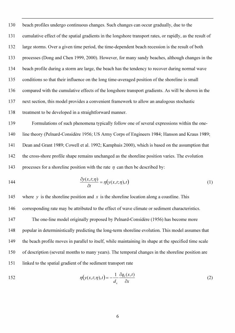
Formulations of such phenomena typically follow one of several expressions within the one-139 line theory (Pelnard-Considère 1956; US Army Corps of Engineers 1984; Hanson and Kraus 1989; 140 Dean and Grant 1989; Cowell et al. 1992; Kamphuis 2000), which is based on the assumption that 141 the cross-shore profile shape remains unchanged as the shoreline position varies. The evolution 142 processes for a shoreline position with the rate η can then be described by: 143

( )ttxyttxy ),;,();,( ηηη =

∂∂ (1) 144

where y is the shoreline position and x is the shoreline location along a coastline. This 145

corresponding rate may be attributed to the effect of wave climate or sediment characteristics. 146 The one-line model originally proposed by Pelnard-Considère (1956) has become more 147

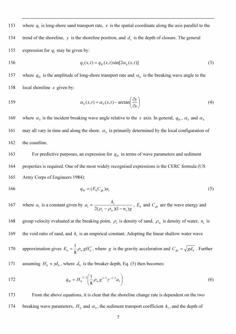
popular in deterministically predicting the long-term shoreline evolution. This model assumes that 148 the beach profile moves in parallel to itself, while maintaining its shape at the specified time scale 149 of description (several months to many years). The temporal changes in the shoreline position are 150 linked to the spatial gradient of the sediment transport rate 151

( ) xtxq

dttxy∂

∂−= ),(1),;,( l

cηη (2) 152

7

where lq is long-shore sand transport rate, x is the spatial coordinate along the axis parallel to the 153

trend of the shoreline, y is the shoreline position, and cd is the depth of closure. The general 154

expression for lq may be given by: 155

)],(2sin[),(),( bl0l txtxqtxq α= (3) 156

where l0q is the amplitude of long-shore transport rate and bα is the breaking wave angle to the 157

local shoreline x given by: 158

∂∂−= xytxtx arctan),(),( 0b αα (4) 159

where 0α is the incident breaking wave angle relative to the x axis. In general, l0q , 0α and bα 160

may all vary in time and along the shore. bα is primarily determined by the local configuration of 161

the coastline. 162

For predictive purposes, an expression for l0q in terms of wave parameters and sediment 163

properties is required. One of the most widely recognised expressions is the CERC formula (US 164 Army Corps of Engineers 1984): 165

1gbbl0 )( aCEq = (5) 166

where 1a is a constant given by gnka )1)((2 sws

11

−−=

ρρ, bE and gbC are the wave energy and 167

group velocity evaluated at the breaking point, sρ is density of sand, wρ is density of water, sn is 168

the void ratio of sand, and 1k is an empirical constant. Adopting the linear shallow water wave 169

approximation gives 2bwb 8

1 gHE ρ= , where g is the gravity acceleration and bgb gdC = . Further 170

assuming bb dH γ≈ , where bd is the breaker depth, Eq. (5) then becomes: 171

= −

12/12/3

w2/5

bl0 81 agHq γρ (6) 172

From the above equations, it is clear that the shoreline change rate is dependent on the two 173

breaking wave parameters, bH and 0α , the sediment transport coefficient 1k , and the depth of 174

8

closure cd . The breaking wave parameters can be calculated from the offshore wave height, period 175

and angle using a wave transformation model, such as SWAN, described by Booij et al. (1999) and 176 Ris et al. (1999). 177

The reliability of the CERC formula for predicting beach morphology has been discussed over 178 many years (Kamphuis 2000). Greer and Madsen (1978) were early reviewers who recommended 179 the formula to be used for the order estimate only. The focus of the discussions is the value of the 180

constant 1k . Schooness and Theron (1994) discussed the relation of the value of 1k with the grain 181

size. Most of the data available for calibrating the empirical one-line formulations is obtained from 182 field measurements. Field measurements in the dynamic surf zone are non-controllable and non-183 repeatable, which may lead to large uncertainties. Pilkey and Cooper (2002) stressed that 184 discrepancies often exist between field data and theoretical predictions due to more or less intense 185 environmental fluctuations. Kamphuis (2000) also criticised the overestimates that come from the 186

CERC expression and suggested the sediment transport rates are proportional to 2bH and 187

{ } 6.0b )],(2sin[ txα . In such situations, researchers should resort to SDEs or other probabilistic 188

models to explore the uncertainty of ‘real’ solutions. These approaches can reveal how both 189 variability and uncertainty in input conditions is transferred to a range of predicted shoreline 190 positions, which makes it possible to establish confidence limits and determine the statistical 191 distribution of the future shoreline position. 192

2.2 Formulation of the stochastic shoreline evolution model 193 Assuming that the evolutionary rate η is one of a collection of admissible change rates η , the 194

evolution uncertainty is thus introduced into the shoreline by the variability of the change rates. 195 This corresponding phenomenon may be attributed to the effect of wave climate differences or 196 sediment characteristics, such as the randomness in input parameters (breaking wave height, period 197

and angle) and uncertainties in the model parameters (sediment transport coefficient 1k and the 198

closure depth cd , etc.). The evolution rates and position variability may also be affected by the 199

9

boundary and initial conditions (e.g., initial shoreline position). With this assumption of a family of 200 admissible change rates and the associated probability distribution of the shoreline position at any 201

time, one thus obtains my , an expectation of the shoreline, with location x at time t . Hence, the 202

corresponding differential equation for mean change dynamics 203

( )ttxyttxy ),;,();,(

mm ηηη =∂

∂ (7) 204

is one of reasonable descriptions of shoreline changes. The following will discuss how the 205 expectation of the shoreline position via a derivative PDF of the shoreline position can be achieved. 206

For a long-term perspective, the morphological response to storms is analogous to ‘noise’ 207 around the long-term trend, which is caused by the fluctuating morphological forcing of the waves, 208 tides and surges. The time-varying uncertainties in shoreline position estimation can be typically a 209 combination of source accuracy (e.g., georeferencing), interpretation error (e.g., field mapping 210 techniques), and natural short-term variability consisting of both shore-term beach changes and 211 variations in water level prior to data collection (Ruggiero and List 2009). Additionally, the 212 geographical surface features are generally determined from remotely sensed data and field 213 measurements. The outcomes of these assessments can raise matching and omission errors, as 214 discussed by Fernandes da Silva and Cripps (2008). Thus, the initial shoreline position 0y is treated 215

as a random variable to account for the uncertainties caused by the short-term variations in either 216 the bed levels or water levels in extracting the initial shoreline position from chart or survey data. 217

Assuming the randomness of the longshore transport is entirely due to the randomness in the 218

breaking wave height means that the empirical coefficient 1k and the closure depth cd and 0α of 219

above one-line model are taken as constants in formulating the simple SDE model; these parameters 220 can also be treated as random, which will be discussed later. As the longshore transport rate is 221

explicitly dependent on 2/5bH , it is convenient to introduce another random parameter defined as 222

2/5bw HH = . 223

10

Therefore, the shoreline position 0y is a random variable at 0t that considers the uncertainties 224

in measurement and short-term variations. These uncertainties will change over time when the 225 shoreline position evolves over time following with an empirical expression (such as the one-line 226

model). In other words, ),( txy is one of a collection of stochastic variables dependent on time t ; 227

therefore, ),( txy is a stochastic process. Moreover, the evolutionary shoreline position can, most 228

rationally, be written in the form of differential equations with random initial conditions (Soong 229 1973; Gardiner 2004): 230

==

)()0,(),,(d

),(d

0

w

xyxyHxyt

txy η (8) 231

where η is an operator of the shoreline position evolving over time that is subject to random 232

breaking wave action for a prescribed random initial shoreline position 0y . This dynamic system 233

with the operator and random initial conditions describes the evolutionary shoreline position as a 234 stochastic process rather than a variable one (Sobczyk 1991; Vanem et al. 2012). 235

Stochastic equations associated with these random processes can be used for a wide class of 236 random excitations with finite correlation time, especially for excitations which can be represented 237 as a response of coastal dynamical systems to a white noise excitation where the Markov process 238 theory can be used (Sobczyk 1991). Substituting the longshore transport model to Eq. (8) gives 239

),(d),(d

w tyHttxy φ−= (9) 240

where ),( tyφ is defined by xdagty∂

∂= −)2sin(1

81),( b

c1

2/12/3w

αγρφ . 241

Before admitting key resources of uncertainty from wH into the above equation, it is worth 242

recalling the method of the description of the statistical characteristics of the wave height. The 243 distributions of the characteristic wave parameters are usually obtained either from measurements 244 or from hindcast waves based on wind data. The distributions of significant wave height have been 245 shown to be well modelled by a log-normal distribution (Jasper 1956; Guedes Soares et al. 1988) 246

11

and a Weibull distribution (Battjes 1972; Guedes Soares and Henriques 1996). Guedes, Soares and 247 Ferreira (1995) proposed a parametric model for the long-term data that adopts the Box-Cox 248 transformation (Box and Cox 1964) to transform the data set into a normal one and then fits the 249 transformed data to a normal distribution to reduce the introduction of additional uncertainties from 250 fitting the data with various parametric distributions. Other distributions have also been used to fit 251 significant wave height (Guedes Soare 2003). Although real data seldom perfectly support the 252 Gaussian assumption for the long-term trends of significant wave height, the theory associated with 253 the Gaussian process is very well understood (Gardiner 2004) and has a vast amount of available 254 tools (Asmussen and Glynn 2007; Rychilk et al. 1997), which led to the decision to adopt a 255 Gaussian white noise model as a first approximation to the random variations of wave excitation. 256 As stated by Sobczyk (1991) and Vanem et al. (2012), the noise forcing term confirms a zero-mean 257 Gaussian distribution, with an identical variance, and assumed independent in space and time. This 258 model may be relatively accurate when only small variability exists in the stationary excitation of 259 breaking wave heights where the physics sets in a limited period (Vanem 2010). We will return to 260 this issue later in the paper. 261

If the stochastic processes of wave excitation are assumed to act as Gaussian white noise 262

(Sobczyk 1991; Vanem et al. 2012), the random variations of wH can be split into two parts: 263

)(mw tWKH += (10) 264

where mK is the mean value of wH and )(tW is a Gaussian white noise process with a mean of 265

zero and a variance of D , which is defined as mvKCD = with 10 v ≤≤ C . In other words, the wave 266

height wH is independently distributed by Gaussian random variables for each t with mean mK 267

and variance D . The driving process )(tW appears to be the pathwise derivative of a Gaussian 268

white noise process, )(d tW , with { } 0)(dE =tW and [ ]{ } tDtW d2)(dE 2= . 269

This pragmatic choice of wave excitation with the Gaussian processes is also considered 270 reasonable because the long-term shoreline position distribution is not controlled by the tail 271

12

distribution of the wave parameter, as in the case of storm-induced erosion, but rather is controlled 272 by the cumulative longshore transport due to the overall wave climate. 273

After adopting Gaussian white noise in the wave height, the evolutionary shoreline position 274 will be characterised by a Markovian process (Horsthemke and Lefever 1984), which can be written 275 as 276

),0(~)();,()]([d),(d

m DNtWtytWKttxy φ+−= (11) 277

where ),0( DN denotes for a normal distribution with zero mean and variance D . 278

The decomposition of Eq. (11) can be recast in the standard form of the stochastic Itô equation 279 (see Soong 1973): 280

)(),(),(d),(d

m tWtyGKtyttxy

+−= φ (12) 281

where ),(),( tytyG φ= . Though ),( tyG and ),( tyφ behave as the same expression, maintaining the 282

initial symbol here can be a smart move when describing the individual contributions of the drift 283 term and the diffusion term. 284

A simple physical interpretation of the model is that the sediment flux consists of two 285 components, a mean flux and a random flux. The former is similar to the original, deterministic 286 one-line model and determines the average evolution rate (the first moment of the rate of change in 287 position), while the latter controls the variability in the evolution rate of the individual shoreline 288 position (the second moment of the rate of change in position). Furthermore, the diffusion Markov 289 process described by the Itô stochastic equations enables us to access the existing analytical and 290 numerical methods for many practical problems (Spencer and Bergman 1993). For instance, the 291 stochastic Itô equation can be performed by Monte Carlo simulations (Kloeden and Platen 1992) to 292 obtain the shoreline trajectories, which is out of great interest here. As discussed by Soong (1973) 293 and Gardiner (2004), the stochastic Itô equation is satisfied the following FP equation 294

[ ] [ ]),()),(),((21),(),(),(

2

2

m typtyDGtyGytypKtyyttyp T

∂∂+

∂∂=

∂∂ φ (13) 295

13

to obtain the expressions for the evolutionary PDF of the shoreline position that was carefully 296 derived in (Soong 1973), among numerous other places and was subsequently studied in many 297 references (Risken 1984; Gradiner 2004). The FP equation describes the evolution of the probability 298 distribution moving forward in time and therefore satisfies a conservation law, indicating that no 299 probability is lost in the system governed by SDEs and thus, the probability of the trivial event is 300 still 1 (Sura 2003). 301

To solve Eq. (13), the following initial condition and boundary conditions must be imposed 302

)(),( 00 yptyp = (14a) 303

( )( ) 0),(

21),(),(

0),(21),(),(

max

min

maxmmax

minmmin

=∂

∂−

=∂

∂−

=

=

yy

T

yy

T

ytypGDGtypKty

ytypGDGtypKty

φ

φ (14b) 304

where maxy and miny are the maximum and minimum shoreline positions, respectively, that the 305

individual section may attain in any given time period. Observe that the boundary condition in Eq. 306 (14), ),( typ , must satisfy the normalisation condition in any given time 307

∫ =max

min1d),(y

yytyp (15) 308

With such an approach, the statistical characteristics, such as the mean and standard deviation, 309 of the ‘real’ coastal positions can be obtained by 310

∫= max

mind),(),(m

y

yytyyptxy (16) 311

( )∫ −=max

mind),(),( 2

msy

yytypyytxy (17) 312

instead of a single deterministic value. This evaluation yields the mean evolutionary dynamics of 313 shoreline position when running this model for every time increment. Above all, the uncertainties in 314 the change rates are introduced into an entire stretch of coastline in space by applying these 315 evolutionary formulae to each individual section. 316

14

The theoretical upper and lower limits, maxy and miny , need to cover the reasonable 317

distribution range of non-negative probability densities of the shoreline position. The stronger 318

boundary conditions 0),( =±∞ tp are imposed, which implies that the values of y remain finite 319

with a probability of one. This result can be interpreted as having an absorbing barrier placed at 320 infinity for the probability flow. Obviously, this addition will increase the non-necessary computing 321 time due to the increased number of discrete grid points because most of the values are zero. 322 Generalising the previous remark, the rescaled absorbing barriers symmetrically placed at 323

ymyy y∆±= m for each cell can be imposed, i.e., 0),( max =typ and 0),( min =typ ; here, 324

ymyy y∆+= mmax and ymyy y∆−= mmin . my is the mean position and may change over time for 325

each cell along the shore. ym is a positive integer that can be between 100-500, depending on the 326

resolution, to describe the discrete value of the PDF in the cross-shore direction. Thus, maxy and 327

miny vary over cells and with time. 328

3. Numerical results and discussions 329

3.1 Solution procedures 330 The FP equation Eq. (13) is a deterministic nonlinear partial differential equation for which a 331

closed form solution would be intractable; thus, this equation must be solved numerically (Wehner 332 and Wolfer 1983; Spencer and Bergman 1993; Anderson 1995). In this model, a second-order 333 implicit finite difference scheme is used with derivative terms approximated by backward 334 difference in time and central difference in space. The general calculation steps for each time 335 increment are as follows: 336

Step 1. Determine the initial condition, )0,( jyp , )12,3,2,1( y +=∆= mjyjy j K ; here, ym is 337

an integer that defines the absorbing barriers, 12 y +m is total number of nodes in the cross-shore 338

direction and y∆ is the grid increment. This integer can be tentatively chosen based on a large 339

upper limit for y calculated by a deterministic computation before running this model. )0,( jyp 340

15

represents the initial distribution of the shoreline, and the mean of the initial shoreline can then be 341

calculated as )0(my . 342

Step 2. Calculate the shoreline position ),( ki txy based on the one-line model, Eq. (2). Here, ix 343

denotes the position of the thi cell ( K,2,1=i ) and kk tkt ∆= ( K,2,1,0=k ), where kt∆ is the time 344

increment. The mean shoreline position ),(m ki txy is then obtained according to Eq. (16), which is 345

used to update the local breaking angle and the long-shore transport rate. 346

Step 3. Calculate ),( kj tyφ and ),( kj tyG . 347

Step 4. Solve the FP equation (13) for ),( mj typ by the Thomas algorithm (Wang and 348

Anderson 1982), where mm tmt ∆= ( K,2,1,0=m ) and mt∆ is the time step for the FP equation. The 349

time step mt∆ can be chosen as either km tt ∆=∆ or km tt ∆=∆ λ , 1>λ . Both time steps must satisfy 350

the respective Courant stability criteria. 351

Step 5. Update ),(m txy i and ),(s txy i using ),( mj typ according to Eqs. (16) and (17). 352

Repeat steps 2 and 5 for the next time step. 353

3.2 Numerical simulations 354

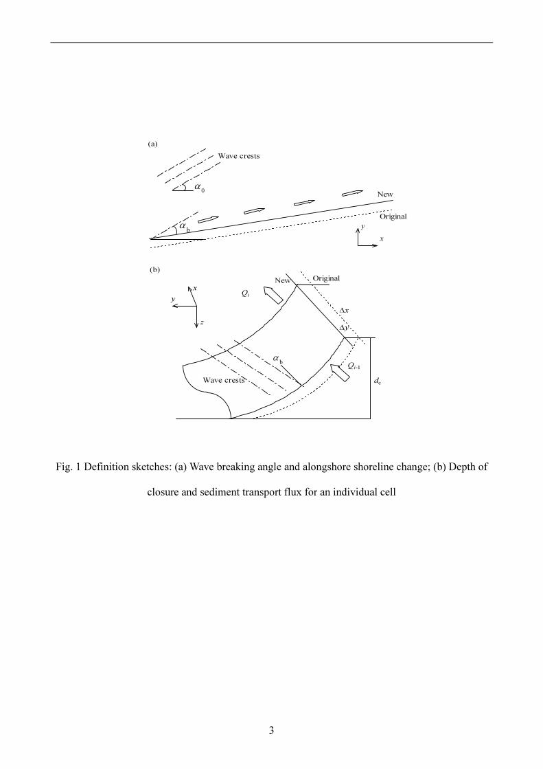
The first test case is a straight sandy shoreline ( )0,(m xy =0) with a long impermeable jetty 355

perpendicular to it at the immediate right of cell 100 with a littoral drift arriving from the left; no 356 by-passing of the jetty occurs. A diagrammatic definition of the main variables is given in Fig. 1. 357 The values used for the constant input variables are given in Table 1. The simulations are performed 358

with a cell width 25=∆x m and a time increment 1.0=∆ kt day. A one year simulation of the 359

shoreline evolution is performed for the boundary condition at 2500=x m, setting 360

btan),0(α=

∂∂

xty , which indicates that the shoreline has an orientation that allows for no sediment 361

transport because no material can pass the structure, i.e., the shoreline normal is in the direction of 362 the waves. The final boundary condition requires that the derivative goes to zero as the beach 363 becomes straight. 364

16

In all simulations, the following variables are used unless stated otherwise (as in the sensitivity 365

tests): mK is 0.375 and vC is 0.15; the mean of the initial shoreline 0y is zero with a standard 366

deviation of 2.5 m in a Gaussian distribution. Considering the maximum deposition distance and to 367

ensure the accuracy of the predictions of the PDFs, =∆y 0.5 m and ym =150 are used in the cross-368

shore direction. 369

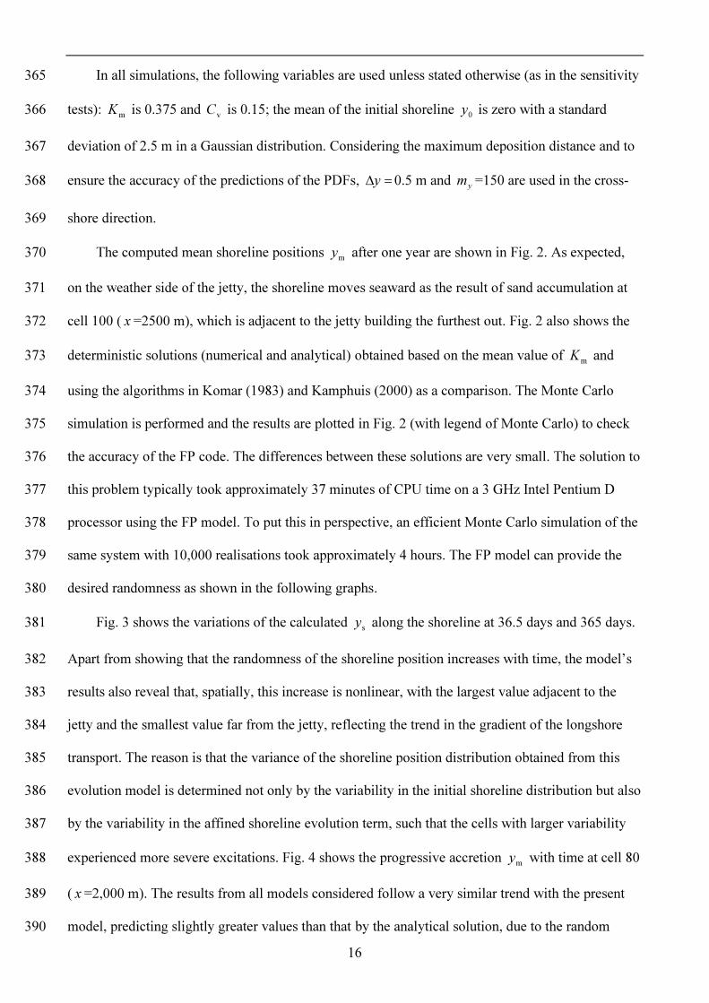
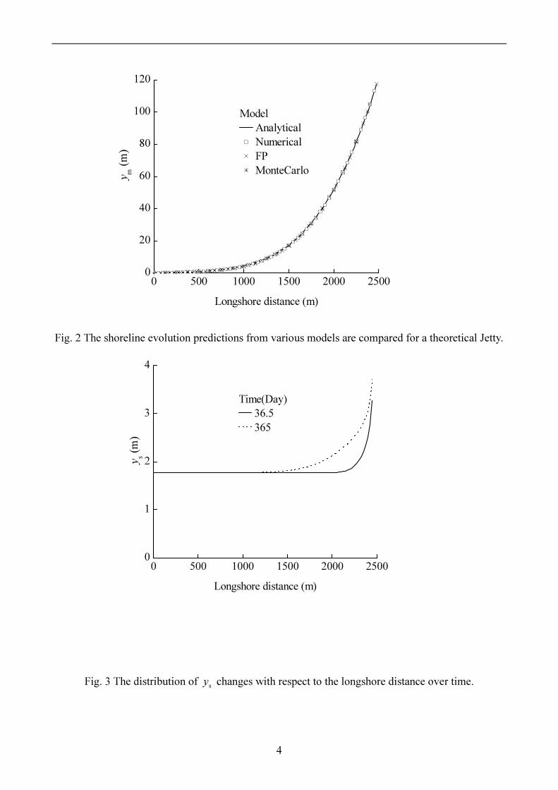
The computed mean shoreline positions my after one year are shown in Fig. 2. As expected, 370

on the weather side of the jetty, the shoreline moves seaward as the result of sand accumulation at 371

cell 100 ( x =2500 m), which is adjacent to the jetty building the furthest out. Fig. 2 also shows the 372

deterministic solutions (numerical and analytical) obtained based on the mean value of mK and 373

using the algorithms in Komar (1983) and Kamphuis (2000) as a comparison. The Monte Carlo 374 simulation is performed and the results are plotted in Fig. 2 (with legend of Monte Carlo) to check 375 the accuracy of the FP code. The differences between these solutions are very small. The solution to 376 this problem typically took approximately 37 minutes of CPU time on a 3 GHz Intel Pentium D 377 processor using the FP model. To put this in perspective, an efficient Monte Carlo simulation of the 378 same system with 10,000 realisations took approximately 4 hours. The FP model can provide the 379 desired randomness as shown in the following graphs. 380

Fig. 3 shows the variations of the calculated sy along the shoreline at 36.5 days and 365 days. 381

Apart from showing that the randomness of the shoreline position increases with time, the model’s 382 results also reveal that, spatially, this increase is nonlinear, with the largest value adjacent to the 383 jetty and the smallest value far from the jetty, reflecting the trend in the gradient of the longshore 384 transport. The reason is that the variance of the shoreline position distribution obtained from this 385 evolution model is determined not only by the variability in the initial shoreline distribution but also 386 by the variability in the affined shoreline evolution term, such that the cells with larger variability 387

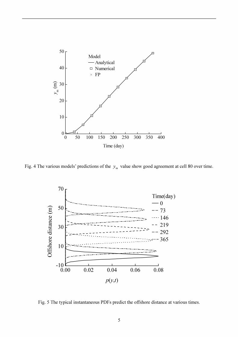
experienced more severe excitations. Fig. 4 shows the progressive accretion my with time at cell 80 388

( x =2,000 m). The results from all models considered follow a very similar trend with the present 389 model, predicting slightly greater values than that by the analytical solution, due to the random 390

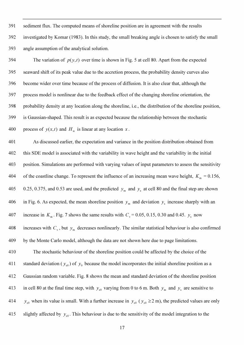
17

sediment flux. The computed means of shoreline position are in agreement with the results 391 investigated by Komar (1983). In this study, the small breaking angle is chosen to satisfy the small 392 angle assumption of the analytical solution. 393

The variation of ),( typ over time is shown in Fig. 5 at cell 80. Apart from the expected 394

seaward shift of its peak value due to the accretion process, the probability density curves also 395 become wider over time because of the process of diffusion. It is also clear that, although the 396 process model is nonlinear due to the feedback effect of the changing shoreline orientation, the 397 probability density at any location along the shoreline, i.e., the distribution of the shoreline position, 398 is Gaussian-shaped. This result is as expected because the relationship between the stochastic 399

process of ),( txy and wH is linear at any location x . 400

As discussed earlier, the expectation and variance in the position distribution obtained from 401 this SDE model is associated with the variability in wave height and the variability in the initial 402 position. Simulations are performed with varying values of input parameters to assess the sensitivity 403

of the coastline change. To represent the influence of an increasing mean wave height, mK = 0.156, 404

0.25, 0.375, and 0.53 are used, and the predicted my and sy at cell 80 and the final step are shown 405

in Fig. 6. As expected, the mean shoreline position my and deviation sy increase sharply with an 406

increase in mK . Fig. 7 shows the same results with vC = 0.05, 0.15, 0.30 and 0.45. sy now 407

increases with vC , but my decreases nonlinearly. The similar statistical behaviour is also confirmed 408

by the Monte Carlo model, although the data are not shown here due to page limitations. 409 The stochastic behaviour of the shoreline position could be affected by the choice of the 410

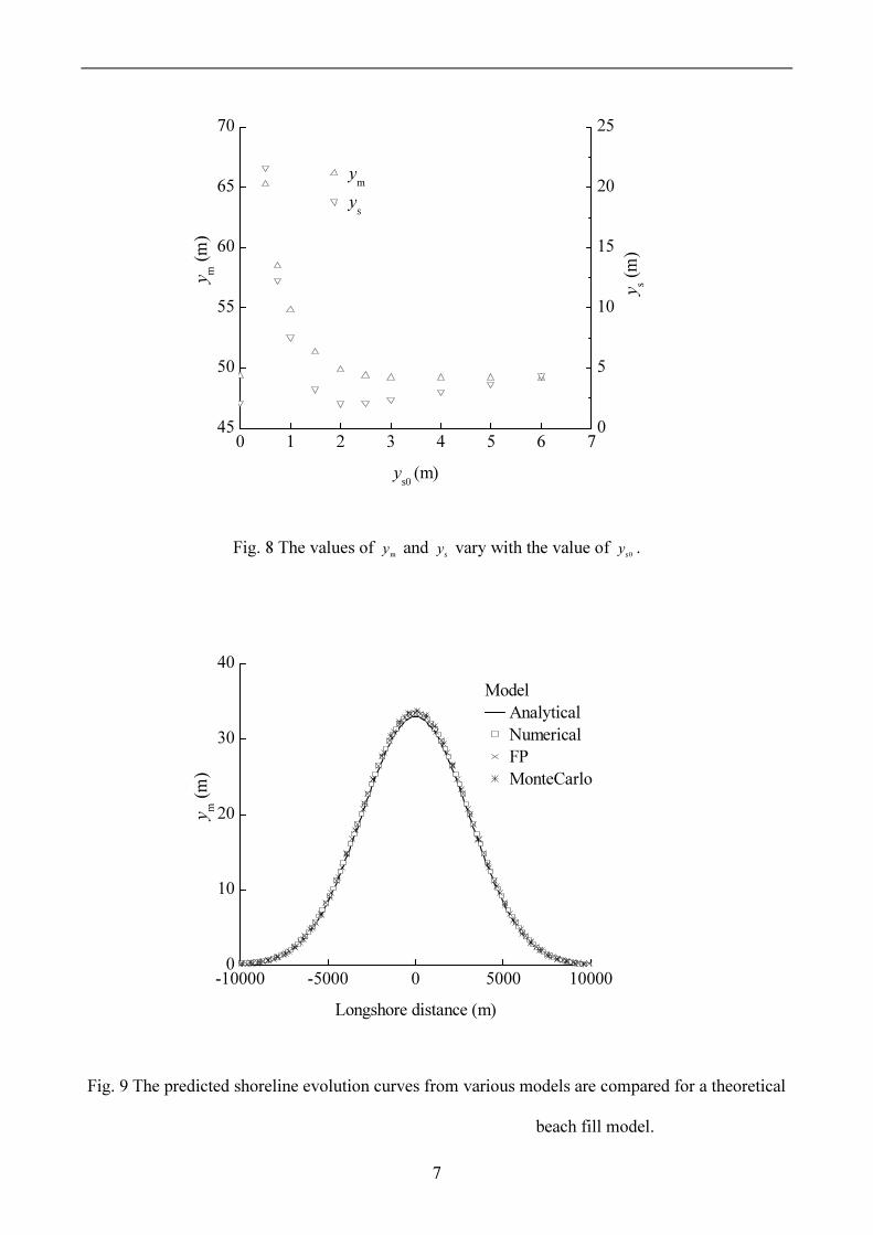
standard deviation ( 0sy ) of 0y because the model incorporates the initial shoreline position as a 411

Gaussian random variable. Fig. 8 shows the mean and standard deviation of the shoreline position 412

in cell 80 at the final time step, with 0sy varying from 0 to 6 m. Both my and sy are sensitive to 413

0sy when its value is small. With a further increase in 0sy ( ≥0sy 2 m), the predicted values are only 414

slightly affected by 0sy . This behaviour is due to the sensitivity of the model integration to the 415

18

numerical resolution of the initial PDF of the shoreline 0y . For a given discretisation, y∆ , the PDF 416

of 0y with a larger 0sy can be better resolved, resulting in a smoother PDF curve of 0y . When 0sy 417

is zero, shown in the left hand side of Fig. 8, the initial shoreline position is a fixed constant with no 418 fluctuations (i.e., without considering the influence of initial random input). Thus, the mean value 419 of the shoreline position is quite close to the result by analytical models, and the deviation of the 420 shoreline position is not quite as large as the results from the diffusion term based on the FP 421 equation. 422

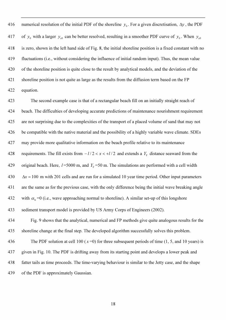
The second example case is that of a rectangular beach fill on an initially straight reach of 423 beach. The difficulties of developing accurate predictions of maintenance nourishment requirement 424 are not surprising due to the complexities of the transport of a placed volume of sand that may not 425 be compatible with the native material and the possibility of a highly variable wave climate. SDEs 426 may provide more qualitative information on the beach profile relative to its maintenance 427

requirements. The fill exists from 2/2/ lxl +<<− and extends a FY distance seaward from the 428

original beach. Here, l =5000 m, and FY =50 m. The simulations are performed with a cell width 429

100=∆x m with 201 cells and are run for a simulated 10 year time period. Other input parameters 430 are the same as for the previous case, with the only difference being the initial wave breaking angle 431

with bα =0 (i.e., wave approaching normal to shoreline). A similar set-up of this longshore 432

sediment transport model is provided by US Army Corps of Engineers (2002). 433 Fig. 9 shows that the analytical, numerical and FP methods give quite analogous results for the 434

shoreline change at the final step. The developed algorithm successfully solves this problem. 435

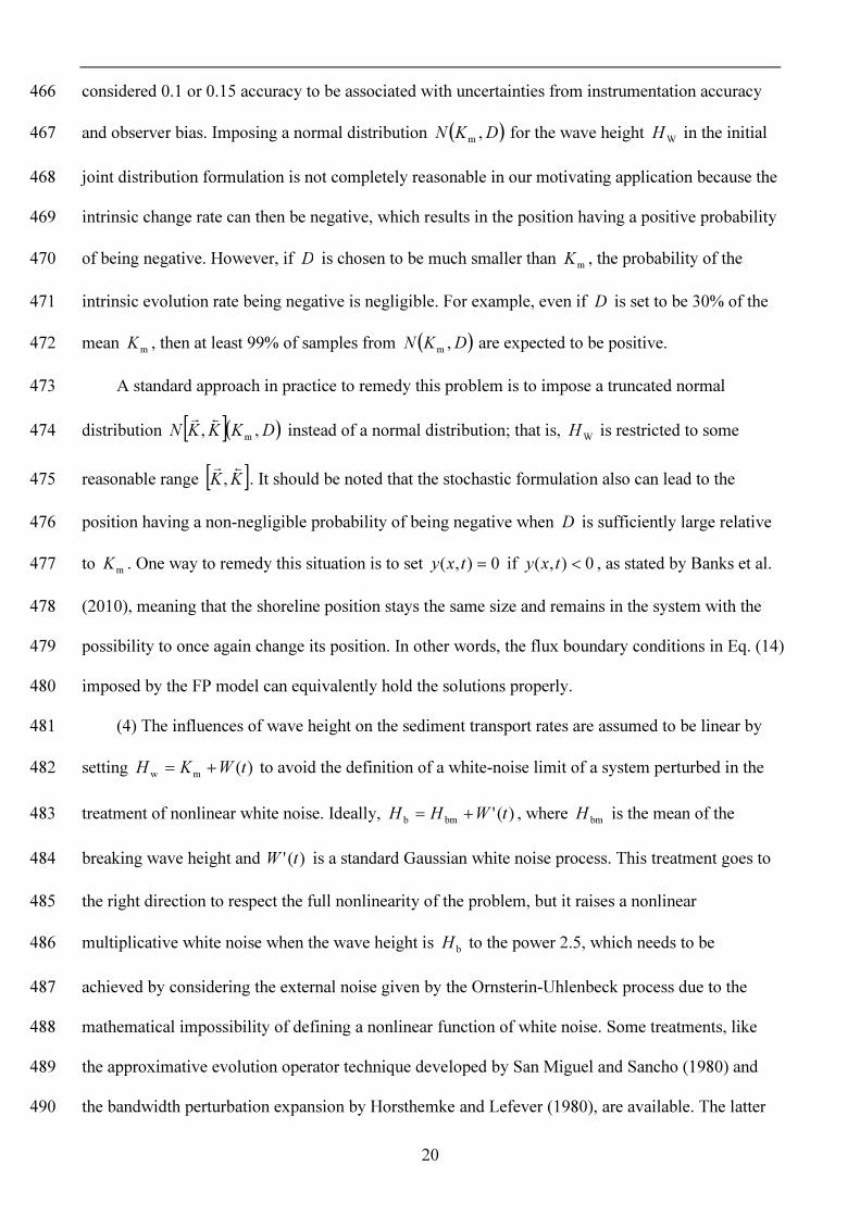
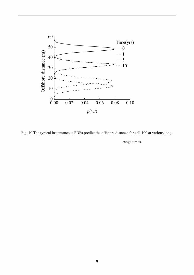
The PDF solution at cell 100 ( x =0) for three subsequent periods of time (1, 5, and 10 years) is 436 given in Fig. 10. The PDF is drifting away from its starting point and develops a lower peak and 437 fatter tails as time proceeds. The time-varying behaviour is similar to the Jetty case, and the shape 438 of the PDF is approximately Gaussian. 439

19

3.3 Discussion 440 (1) While the initial results presented here are encouraging and have demonstrated the ability 441

of the linear breaking wave height scheme to predict the uncertainty in the shoreline evolution in 442 response to uncertainties in the wave parameterisation, these results may not be immediately 443 applicable to all shoreline change model studies. One limitation inherent to the technique as 444 developed is the assumption of Gaussian statistics for the distribution of the random wave height 445 values. This assumption is made for pragmatic reasons in that it allows a simple parameterisation of 446 statistics in terms of the mean and covariance matrices and that the transformation of Gaussian 447 variables is conceptually simple. The effects of different types of distributions on the results of the 448 breaking wave height should be investigated before this model can be applied more widely; it is 449 worth pursuing the outcomes under random input of non-Gaussian distributions, although the 450 associated interpretation of SDEs might be difficult to follow by coastal engineers, as is the case in 451 one of the derivations described by Kontorvich (1995). 452

(2) Knowledge about the theoretical distribution of wave height parameters is limited; thus, 453 other distribution types are usually more attractive, especially for a long-term statistic of extremes. 454 The distributions of significant wave heights have been investigated by a log-normal distribution 455 (Jasper 1956; Guedes Soares et al. 1988). As suggested by Anderson et al. (2001), a Gaussian 456

distribution can be fitted to the logarithms of the values of sH . Hence, the logarithms of the sH 457

values as random variables assuming a Gaussian distribution from this point forward. In other 458

words, if sH is a log-normal random variable, the distribution function of ( )slog H is obviously a 459

normal distribution function. This transition will instantly provoke the antilogarithm or inverse 460

logarithm, such as ( )slog10 H , into the drift function of the stochastic shoreline evolution equation, 461 requiring the determination of its variability or noise intensity. 462

(3) The intensity of a white noise process to wave height, mvKCD = , is a measure of the 463

dispersion of the probability distribution data, which is related to the mean of the wave height. In 464

general, vC will not be larger than 0.5, even though it can be 1.0. Rosati and Kraus (1991) 465

20

considered 0.1 or 0.15 accuracy to be associated with uncertainties from instrumentation accuracy 466

and observer bias. Imposing a normal distribution ( )DKN ,m for the wave height WH in the initial 467

joint distribution formulation is not completely reasonable in our motivating application because the 468 intrinsic change rate can then be negative, which results in the position having a positive probability 469

of being negative. However, if D is chosen to be much smaller than mK , the probability of the 470

intrinsic evolution rate being negative is negligible. For example, even if D is set to be 30% of the 471

mean mK , then at least 99% of samples from ( )DKN ,m are expected to be positive. 472

A standard approach in practice to remedy this problem is to impose a truncated normal 473

distribution [ ]( )DKKKN ,, m

sr instead of a normal distribution; that is, WH is restricted to some 474

reasonable range [ ]KK sr

, . It should be noted that the stochastic formulation also can lead to the 475

position having a non-negligible probability of being negative when D is sufficiently large relative 476

to mK . One way to remedy this situation is to set 0),( =txy if 0),( <txy , as stated by Banks et al. 477

(2010), meaning that the shoreline position stays the same size and remains in the system with the 478 possibility to once again change its position. In other words, the flux boundary conditions in Eq. (14) 479 imposed by the FP model can equivalently hold the solutions properly. 480

(4) The influences of wave height on the sediment transport rates are assumed to be linear by 481

setting )(mw tWKH += to avoid the definition of a white-noise limit of a system perturbed in the 482

treatment of nonlinear white noise. Ideally, )('bmb tWHH += , where bmH is the mean of the 483

breaking wave height and )(' tW is a standard Gaussian white noise process. This treatment goes to 484

the right direction to respect the full nonlinearity of the problem, but it raises a nonlinear 485

multiplicative white noise when the wave height is bH to the power 2.5, which needs to be 486

achieved by considering the external noise given by the Ornsterin-Uhlenbeck process due to the 487 mathematical impossibility of defining a nonlinear function of white noise. Some treatments, like 488 the approximative evolution operator technique developed by San Miguel and Sancho (1980) and 489 the bandwidth perturbation expansion by Horsthemke and Lefever (1980), are available. The latter 490

21

treatment requires the SDE to be interpreted as a Stratonovic equation rather than an Itô one; 491 additionally, the white-noise limit has to be taken with circumspection by intricate derivation, 492 which will stray slightly from the main point of the introduction of a simple SDE to include 493 randomness in the shoreline change simulations. Furthermore, the multiplicative nonlinear external 494 noise should be studied to elucidate the influence of the white-noise description on the nonlinearity. 495 The reader should consult Horsthemke and Lefever (1984) and Gardiner (2004) for details. In the 496 current theoretical studies, this would make any theoretical comparisons in a reasonable way an 497 extremely formidable task. 498

(5) The parameter wave angle 0α appears here in a sine function; thus, it can mathematically 499

handle a random coefficient easily through linearisation of the equation. Actually, the parameter 500 value can be approximated by the first term of its Taylor series if the angle is small, and the SDE Eq. 501 (11) subject to fluctuations from the wave height and the initial breaking angle can be recast by 502

)()0(),()()(),()(),(d),(d

bmm tWtyKtWtytyKttxy ψϕαψϕαψω ++−= (18) 503

where c

12/12/3 1

161),( dagty −

= γρω , xxy

∂

∂∂−∂

=arctan22

)(0mα

αψ and 504

xxy

∂

∂∂−∂

=arctan2

)0(ψ , 0mα is the mean of the initial breaking angle. )(b tW can be 505

approximated by the independent Gaussian white noise fluctuation wave’s initial breaking angle. 506 The product of two white noise functions has been neglected in the above equation, similar to the 507 treatment by Unny and Karmeshu (1984). In this case, the corresponding FP equation can be given 508 by: 509

[ ] [ ]∑= ∂

∂+∂∂=

∂∂ 2

12

2

m ),()21),()(),(),(

i

Tiii typDytypKtyyt

typ ηηαψω (19) 510

22

where )(),(1 αψωη ty= and )0(),(m2 ψωη tyK= . By analogy to other parameters, such as 1k and 511

cd , there must exist an analogous FP equation to be solved when applying the independent 512

Gaussian white noise term in SDE. 513 It should be noted that the incident wave angle is assumed to be constant in working examples, 514

which may not be the case on a real coast, especially near a jetty or a barrier, which experience the 515 greatest wave exposure and the most severe sediment transport. A deliberate analysis needs to be 516 performed by incorporating a wave transformation model. 517

(6) All numerical models have some degree of model imperfection because no empirical 518 equation can exactly reproduce nature. In the present SDE model, storm-induced shoreline change 519 and subsequent beach recovering are assumed to “average out” over the long term, e.g., the 520 breaking wave data are calculated from averaged or statistical offshore wave data. So the emphasis 521 of this paper is on the long-term evolution of alongshore transport rather than on seasonal or storm-522 based evolution; thus, the forces resulting from wave conditions can only be considered as averages 523 of this force for the ensemble. Surely, if recorded data are available for a wave storm and are taken 524 as a certain input, predicting the probability density of the shoreline position for one extreme wave 525

storm by considering some other parameters as random coefficients, 1k or cd , is not difficult. 526

(7) Additive noise can be incorporated to represent the model error and can be derived from 527 other fluctuations sources without any inconvenience. Actually, the Liouville model can also solve 528 this multiplicative white noise problem (Kubo 1963; Gardiner 2004). A SDE model based on the 529 Liouville equation can be developed for the non-linear random dynamics systems in which the 530 erosion process is based on the one-line type model and the random effects are assumed to be 531 characterised by random variables, which also permit non-Gaussian distributions for the breaking 532 wave parameter. These results will be reported separately. 533

(8) The solving procedure of the FP equation is the same as the formation with a general 534 second-order parabolic partial differential equation. A second-order or higher-order implicit 535 difference approximation with the backward in time and central in space method can be used. The 536

23

accuracy of the numerical method will increase the accuracy with the exact probability density, i.e., 537 another analytical solution of the FP equation need to be addressed, although it is not of great 538 interest here. 539

(9) A simple CERC law is employed because it provides (general, non-unique) empirical fits to 540 field data sets and is popular in shoreline dynamic models. The ideas presented here are also 541 tractable with other forms of empirical laws, but these generalisations will not be pursued here. 542

4. Conclusions 543

Uncertainty is introduced into the coastal morphological processes for each cell along the 544 coastline by recasting an Itô SDE by considering the stochastic nature of forces and the initial 545 shoreline position. Accordingly, the FP model associated with the Itô SDE is formulated as an 546 explicit expression of the PDF of the shoreline positions. The mean evolutionary dynamics of the 547 time-dependent shoreline position, updated from their PDFs each time increment, is driven by a 548 mature deterministic framework. The numerical accuracy of the model has been confirmed by 549 comparison of the mean shoreline predicted by the present model with that from the deterministic 550 and Monte Carlo simulations approaches. The effect of the input parameters on the predicted 551 shoreline statistical properties is evaluated through a series of sensitivity analyses. The proposed 552 model is able to account for the effects of uncertainties in the breaking wave parameter and the 553 initial shoreline position and provides an efficient means of predicting the complete stochastic 554 characteristics of shoreline evolution without requiring a Monte Carlo sampling. 555

Compared to the conventional predictions based solely on deterministic solutions, the analyses 556 here provide a reasonable foundation by admitting uncertainty, and the confidence limits and 557 statistical characteristics of the future shoreline position can be established. The statistics of 558 coastline position are not stationary with respect to either space or time. The present work adopts a 559 simple representation of the breaking wave climate such that the random variability of the breaking 560 wave angle is neglected for the sake of simplicity. A detailed development and application to a few 561

24

real sites should be encouraged to further account for the spatial variation of the breaking wave 562 height parameters and the multi-dimensional sediment transport pathways. 563

Acknowledgements 564

This research is supported by the UK Engineering and Physical Science Research Council as 565 part of Grant No GR\L53953. 566

Appendix A The theoretical framework for a general 567 stochastic system 568

For a real field site where sediment transport pathways are parallel or shore-normal (both have 569 significant components in two or three dimensions), the simplification made by the one-line 570 alongshore model is unlikely to produce an accurate prediction for the variability of the coastal 571 spatial configurations. In this case, a multi-dimensional deterministic numerical model can be 572 incorporated into this modelling framework, involving a stochastic process of an initial state and 573 some model parameters along these lines. For such a random dynamic coastal system, a more 574 specific model that characterises a Markovian process is often adopted, which is obtained by a 575 decomposition as the similar formulation with Eq. (12): 576

)(),(),(),( ttttx WYGYκY +=& (A1) 577

where T21 ),,,(

dnYYY K=Y is the state vector, dn is the dimension of the state space, ),( tYκ is a 578

function vector representing the effects of some form of drift, ),( tYG is a function vector 579

representing the effects of random diffusion, and )(tW is a en -dimensional Gaussian (or white) 580

noise vector. Assuming that the white noise processes are mutually independent, the co-variance 581

parameter matrix of )(tW will be a diagonal matrix with its diagonal terms equal to the variance of 582

the white noise processes )(,),(),(e21 tWtWtW nK and ),,,(

ee2211 nnDDD K=D . 583

Eq. (A1) can also be written in the vector form of the standard Itô equation (see Soong 1973): 584

)(d),(d),(),(d tttttx WYGYκY += (A2) 585

25

with { } 0W =)(d tE and [ ]{ } ttE d2)(d 2 DW = . 586

The dynamical system described by Eq. (A2) with the deterministic operators κ and G driven 587 by some expressions of sediment transport, the evolutionary PDFs of the shoreline position Y , 588

),( tp y , will satisfy the FP equation (Soong 1973; Gardiner 2004): 589

[ ] [ ]∑∑== ∂∂

∂+∂∂−=

∂∂ dd

1,

20 )(2

1),(),,( n

vuuv

T

uv

n

vjv

vpGDGyyptyyt

ttpη

yy (A3) 590

The term uvGDG )( T is given by: 591

),,2,1,(,),,2,1,(

),(),()(

ed

1,

T e

nlknvutyGtyGDGDG

n

lkvlukkluv

KK ==

= ∑= (A4) 592

where ukG and vlG are components of ),( tyG . 593

The theoretical framework described above is formulated into a stochastic shoreline evolution 594

model to use for a dn -dimensional SDE with a en -dimensional Wiener process. In these working 595

examples, the state function vector is derived using the one-line model, which means that only 596

longshore transport is considered to contribute to the shoreline changes, implying 1d =n . For 597

simplicity’s sake, only the characteristic wave height parameter is taken as a random parameter, 598

implying 1e =n . 599

Notations 600

1a Constant in the expression for l0q [ kgsecm 22

];

gbC wave group celerity [m/s]; vC coefficient of variance, 10 v ≤≤ C , defined as the ratio of the

standard deviation to the mean; d difference operator; D variance vector; bd breaker depth [m]; cd closure depth [m]; ijD thi row and thj column component of D ; E expectation operator; bE wave energy evaluated at the breaking point [ kN ];

26

g acceleration due to gravity [ 2sec/m ]; G deterministic operator of Itô equation; bh discrete wave height at breaking [m]; bH wave height at breaking [m]; bmH mean of bH ; sH significant wave height [m];

i alongshore cell number; j cross-shore node number; k time step of shoreline model; m time step of FP model; 1k

sediment transport coefficient or dimensionless empirical coefficient;

mK mean of wH ; l distance alongshore [m];

ym number of the discrete distribution in cross-shore direction; N normal distribution; dn dimension of state space; en number of random parameters; sn void ratio of sand; p probability density function; 0p initial of p ; lq volumetric long-shore sediment transport rate [ /secm3 ]; l0q

amplitude of volumetric long-shore sediment transport rate [ /secm3 ];

t time [sec]; T transpose of a matrix; 0t initial time [sec]; kt time in thk step of one-line shoreline model [sec]; mt time in thm step [sec] of Thomas algorithm; W Wiener process vector; bW Gaussian White noise of wave initial breaking angle; iW thi component of Wiener process W ; 'W Standard Gaussian White noise process of bH ; x distance alongshore [m]; y shoreline position in cross-shore direction [m]; y discrete stochastic process vector; Y stochastic process or random variable of shoreline position or

random state (which is a component of the state vector); Y stochastic process vector;

0y initial y ; 0Y initial random state or random variable of shoreline position

Y ; 0Y initial Y ; FY extension distance seaward from the rectangular beach; iy thi component of y ; my mean of y ;

27

mY expected value or mean value of Y ; maxy maximum discrete shoreline position; miny minimum discrete shoreline position; sy standard deviation of y ; sy standard deviation of y ;

Y& time derivative of Y ; 0α incident angle of breaking waves relative to x [deg]; 0mα mean of incident angle of breaking waves relative to x

[deg]; bα Wave angle at the point of breaking [deg]; γ ratio of wave height to water depth at breaking,

bbd

H= ;

kt∆ time increment of one-line shoreline model [sec]; mt∆ time increment of Thomas algorithm [sec]; x∆ size increment in along-shore direction [m]; y∆ size increment in cross-shore direction [m]; η

operator vector of determination of a dynamical state, may be determined by an appropriate deterministic shoreline evolution model;

iη thi component of the operator η ; κ vector of drift; iκ thi component of κ ; λ ratio,

k

m

tt

∆∆= ;

sρ mass density of the sediment grains [ 3kg/m ]; wρ mass density of water [ 3kg/m ];

φ xdag∂

∂= −)2sin(1

81 b

c1

2/12/3w

αγρ ;

ψ x

xy

∂

∂∂−∂

=arctan22 0mα

;

ω c

12/12/3

w1

81

dag −

= γρ . 601

References 602

Anderson CW, Carter DJT, Cotton PD (2001) Wave climate variability and impact on offshore 603 design extremes. Report prepared for Shell International, 2001 604

Anderson JD (1995) Computational Fluid Dynamics: The Basics with Applications. McGrawHill 605

28

Asmussen S, Glynn PW (2007) Stochastic simulation. Algorithms and analysis. Springer-Verlag. 606 Stochastic modelling and applied probability. pp 306–324 607

Banks HT, Davis JL, Ernstberger SL, Hu S, Artimovich E, Dhar AK, Browdy CL (2010) A 608 comparison of probabilistic and stochastic formulations in modeling growth uncertainty and 609 variability. J Biol Dyn 3:130–148 610

Battjes JA (1972) Long-term wave height distribution at seven stations around the British Isles. 611 Deutsche Hydrographische Zeitschrift J 25:179–189 612

Bayram A, Larson M, Miller HC, Kraus NC (2001) Cross-shore distribution of longshore sediment 613 transport: Comparison between predictive formulas and field measurements. Coast Eng 44:79–99 614

Benassai E, Calabrese M, Sorgenti degli Uberti G (2001) A probabilistic prediction of beach 615 nourishment evolution. MEDCOAST01, The 5th International Conference on the Mediterranean 616 Coastal Environment, October 23–27, 2001, Yasmine Beach Resort, Hammamet, Tunisia 617

Bodo BA, Thompson ME, Unny TE (1987) A review on stochastic differential equations for 618 applications in hydrology. Stoch Hydrol Hydraul 1:81–100 619

Booij N, Ris RC, Holthuijsen LH (1999) A third-generation wave model for coastal regions, 1, 620 model description and validation. J Geophys Res 104(C4):7649–7666 621

Box GEP, Cox DR (1964) An analysis of transformations. J Royal Stat Soci 26(B):2ll–252 622

Camfield FE, Morang A (1996) Defining and interpreting shoreline change. Ocean Coast Manage 623 32:129–151 624

Cowell PJ, Roy PS, Jones RA (1992) Shoreface translation model: computer simulation of coastal-625 sand-body response to sea level rise. Math Comput Simulat 33:603–608 626

Cowell PJ, Roy PS, Jones RA (1995) Simulation of large scale coastal change using a 627 morphological behaviour model. Mar Geol 126:45–61 628

Cowell PJ, Thom BG, Jones RA, Everts CH, Simanovic D (2006) Management of uncertainty in 629

29

predicting climate-change impacts on beaches. J Coast Res 22:232–245 630

Davies AG, van Rijn LC, Damgaard JS, van de Graaff J, Ribberink JS (2002) Intercomparison of 631 research and practical sand transport models. Coast Eng 46:1–23 632

De Vriend H, Capobianco M, Chesher T, Swart HE, Latteux B, Stive M (1993) Approaches to long-633 term modelling of coastal morphology: a review. Coast Eng 21:225–269 634

Dean RG, Grant J (1989) Development of methodology for thirty-year shoreline projections in the 635 vicinity of beach nourishment projects, UFL/COEL-89/026. Gainesville, University of Florida 636

Dong P, Chen H (1999) Probabilistic predictions of time dependent long-term beach erosion risks. 637 Coast Eng 36:243–261 638

Dong P, Chen H (2000) A simple life-cycle method for predicting extreme shoreline erosion. Stoch 639 Environ Res Risk Assess 14:79–89 640

Dostal L, Kreuzer E (2011) Probabilistic approach to large amplitude ship rolling in random seas. 641 Proc Inst Mech Eng Part C: J Mech Eng Sci 225:2464–2476 642

Fernandes da Silva PC, Cripps JC (2008) Comparing directional line sets using non-parametric 643 statistics: a new approach for geoenvironmental applications. Stoch Environ Res Risk Assess 644 22:231–246 645

Gardiner CW (2004) Handbook of Stochastic Methods: For Physics, Chemistry and the Natural 646 Sciences, 3rd ed., Springer-Verlag, Berlin, New York 647

Greer MN, Madsen OS (1978) Longshore sediment transport data: a review. Proc 16th Int Conf on 648 Coastal Engrg Hamburg. pp 1563–1576 649

Guedes Soares C (2003) Probabilistic models of waves in the coastal zone. Advances in coastal 650 modeling. pp 159–187 651

Guedes Soares C, Ferreira JA (1995) Modelling long-term distributions of significant wave height. 652 Proceedings of the 14th International Conference on Offshore Mechanics and Arctic Engineering, 653

30

ASME, New York. pp. 5l–61 654

Guedes Soares C, Henriques AC (1996) Statistical uncertainty in long-term distributions of 655 significant wave height. J Offshore Mech Arctic Eng 11:284–291 656

Guedes Soares C, Lopes LC, Costa M (1988) Wave climate modelling for engineering purposes. In: 657 Schrefer and Zienkiewicz (Editors), Computer Modelling in Ocean Engineering, pp. 169–175. The 658 Netherlands: AA Balkema Publishers 659

Hall JW, Meadowcroft IC, Lee EM, Van Gelder PHAJM (2002) Stochastic simulation of episodic 660 soft coastal cliff recession. Coast Eng 46:159–174 661

Hanson H, Kraus NC (1989) GENESIS: Generalized Model for Simulating Shoreline Change, 662 Report 1, Technical Report CERC-89-19. Vicksburg, MS, CERC, US Army WES 663

Horsthemke W, Lefever R (1980) A perturbation expansion for external wide band Markovian 664 noise: Application to transitions induced by Ornstein-Uhlenbeck noise Zeitschrift für Physik B 665 Condensed Matter 40:241–247 666

Horsthemke W, Lefever R (1984) Noise-Induced Transitions Theory and Applications in Physics, 667 Chemistry, and Biology Series: Springer Series in Synergetics 15:65–81 668

Itô K (1951) Multiple Wiener integral. J Math Soc Japan 3:157–169 669

Jasper NH (1956) Statistical distribution patterns of ocean waves and of wave-induced ship stresses 670 and motions, with engineering applications. Transactions of the Society of Naval Architects and 671 Marine Engineers pp. 375–432 672

Kamphuis JW (2000) Introduction to Coastal Engineering and Management. World Scientific 673

Kloeden PE, Platen E (1992) The Numerical Solution of Stochastic Differential Equations. 674 Springer-Verlag 675

Komar PD (1983) Handbook of Coastal Processes and Erosion, CRC Press 676

Kontorovich VY, Lyandres VZ (1995) Stochastic differential equations: an approach to the 677

31

generation of continuous non-Gaussian processes. IEEE Trans Signal Process 43:2372–2385 678

Kubo R (1963) Stochastic liouville equations. J Math Phys 4:174–183 679

Larson M, Kraus NC (1994) Temporal and spatial scales of beach profile change, Duck, North 680 Carolina Mar Geol 117:75–94 681

Pelnard-Considère R (1956) Essai de Theorie de I'Evolution des Formes de Rivage en Plages de 682 Sables et de Galets. Fourth Journess de I’Hydralique, les energies de la Mer Question III, Rapport 1, 683 289–298 684

Pilkey OH, Cooper J, Andrew G (2002) Longshore transport volumes: a critical view. J Coast Res 685 Special Issue 36:572–580 686

Reeve DE, Spivack M (2004) Evolution of shoreline position moments. Coast Eng 51:661–673 687

Ris RC, Holthuijsen LH, Booij N (1999) A third-generation wave model for coastal regions, 2, 688 verification. J Geophys Res 104(C4):7667–7681 689

Risken H (1984) The Fokker-Planck Equation. Springer-Verlag 690

Rosati JD, Kraus NC (1991) Practical Considerations in Longshore Transport Calculations. CETN 691 II-24, U.S. Army Engineer Waterways Experiment Station, Coastal and Hydraulics Laboratory, 692 Vicksburg, MS 693

Ruggiero P, List J, Hanes DM, Eshleman J (2006) Probabilistic Shoreline Change Modeling, 30th 694 International Conference on Coastal Engineering. San Diego, California ASCE pp 3417–3429 695

Ruggiero P, List JH (2009) Improving accuracy and statistical reliability of shoreline position and 696 change rate estimates. J Coast Res 25:1069–1081 697

Rychlik I, Johannesson P, Leadbetter MR (1997) Modelling and statistical analysis of ocean-wave 698 data using transformed Gaussian processes. Marine Struct 10:13–47 699

Sancho JM, San Migue M (1980) External non-white noise and nonequilibrium phase transitions. 700 Zeitschrift für Physik B Condensed Matter 36:357–364 701

32

Schoonees JS, Theron AK (1994) Accuracy and applicability of the SPM longshore transport 702 formula. Proc 24th Int Conf on Coastal Engrg ASCE pp 2595–2609 703

Soong TT (1973) Random Differential Equations in Science and Engineering. New York: 704 Academic Press 705

Southgate HN (1995) The effects of wave chronology on medium and long term coastal 706 morphology. Coast Eng 26:251–270 707

Sobczyk K (1991) Stochastic Differential Equations with Applications to Physics and Engineering. 708 Kluewer, Dordrecht, Boston 709

Spencer Jr, Bergman LA (1993) On the numerical solution of the Fokker-Planck equation for 710 nonlinear stochastic systems. Nonlinear Dynam 4:357–372 711

Stive MJF, Aarninkhof SGJ, Hamm L, Hanson H, Larson M, Wijnberg KM, Nicholls RJ, 712 Capobianco M (2002) Variability of shore and shoreline evolution. Coast Eng 47:211–235 713

Sura P (2003) Stochastic analysis of Southern and Pacific Ocean sea surface winds. J Atmos Sci 714 60:654–666 715

Unny TE, Karmeshu (1984) Stochastic nature of outputs from conceptual reservoir model cascades. 716 J Hydrol 68:161–180 717

US Army Corps of Engineers (1984) Shore protection manual. Coastal Engineering Research 718 Center, Washington, DC 719

US Army Corps of Engineers (2002) Coastal Engineering Manual, Part III, Coastal Sediment 720 Processes, Chapter III-2: Longshore Sediment Transport. US Army Corps of Engineers, 721 Washington, DC 722

Vanem E (2010) Long-term time-dependent stochastic modelling of extreme waves. Stoch Environ 723 Res Risk Assess 25:185-209 724

Vanem E, Huseby AB, Natvig B (2012) A Bayesian hierarchical spatio-temporal model for 725

33

significant wave height in the North Atlantic. Stoch Environ Res Risk Assess 26:609–632 726

van der Berg E, Heemink AW, Lin HX, Schoenmakers JGM (2005) Probability density estimation 727 in stochastic environmental models using reverse representations. Stoch Environ Res Risk Assess 728 20:126–134 729

Vrijling JK, Meijer GJ (1992) Probabilistic coastline position computations. Coast Eng 17:1–23 730

Walton Jr TL (2007) Storm protection beach fill planning on barrier islands. Shore and Beach 731 75:43–48 732

Wang HF, Anderson MA (1982) Introduction to groundwater modeling: finite difference and finite 733 element methods. W H Freeman and Co 734

Wehner MF,Wolfer WG (1983) Numerical evaluation of path integral solutions to the Fokker-735 Planck equations. Physics Review 27:2663–2670 736

1

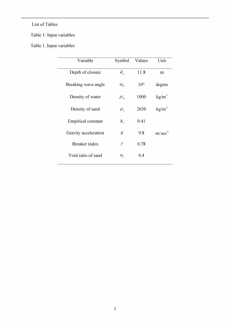
List of Tables Table 1: Input variables Table 1. Input variables

Variable Symbol Values Unit

Depth of closure cd 11.8 m

Breaking wave angle 0α 10° degree

Density of water wρ 1000 3kg/m Density of sand sρ 2650 3kg/m

Empirical constant 1k 0.41

Gravity acceleration g 9.8 2secm/ Breaker index γ 0.78

Void ratio of sand sn 0.4

2

List of Figures Fig. 1 Definition sketches: (a) Wave breaking angle and alongshore shoreline change; (b)

Depth of closure and sediment transport flux for an individual cell. Fig. 2 The shoreline evolution predictions from various models are compared for a theoretical

Jetty.

Fig. 3 The distribution of sy changes with respect to the longshore distance over time.

Fig. 4 The various models’ predictions of the my value show good agreement at cell 80 over

time. Fig. 5 The typical instantaneous PDFs predict the offshore distance at various times.

Fig. 6 The predicted my and sy values vary with different mK input values.

Fig. 7 The values of my and sy vary with vC .

Fig. 8 The values of my and sy vary with the value of 0sy .

Fig. 9 The predicted shoreline evolution curves for various models are compared for a theoretical beach fill model.

Fig. 10 The typical instantaneous PDFs predict the offshore distance for cell 100 at various long-range times.

3

Fig. 1 Definition sketches: (a) Wave breaking angle and alongshore shoreline change; (b) Depth of closure and sediment transport flux for an individual cell

bα

0α

x

yOriginal

New

Wave crests

Qi-1

Qi

∆x∆y

dc

OriginalNew

z

xy

bα

Wave crests

(a)

(b)

4

Fig. 2 The shoreline evolution predictions from various models are compared for a theoretical Jetty.

Fig. 3 The distribution of sy changes with respect to the longshore distance over time.

0 500 1000 1500 2000 25000

20

40

60

80

100

120

y m (m

)

Longshore distance (m)

Model Analytical Numerical FP MonteCarlo

0 500 1000 1500 2000 25000

1

2

3

4

y s (m

)

Longshore distance (m)

Time(Day) 36.5 365

5

Fig. 4 The various models’ predictions of the my value show good agreement at cell 80 over time.

Fig. 5 The typical instantaneous PDFs predict the offshore distance at various times.

0 50 100 150 200 250 300 350 4000

10

20

30

40

50y m

(m)

Time (day)

Model Analytical Numerical FP

0.00 0.02 0.04 0.06 0.08-10

10

30

50

70Time(day)

0 73 146 219 292 365

Offsh

ore di

stanc

e (m)

p(y,t)

6

Fig. 6 The predicted values of my and sy vary with different mK inputs.

Fig. 7 The predicted my and sy values vary with vC .

0.01 0.02 0.03 0.04 0.05 0.0610

20

30

40

50

60

70

1.8

2.0

2.2

2.4

y m (m

)

km

ym

ys

y s (m

)

0.0 0.1 0.2 0.3 0.4 0.549.0

49.2

49.4

49.6

49.8

50.0

2.0

2.2

2.4

2.6

y m (m

)

Cv

ym

ys

y s (m

)

7

Fig. 8 The values of my and sy vary with the value of 0sy .

Fig. 9 The predicted shoreline evolution curves from various models are compared for a theoretical beach fill model.

0 1 2 3 4 5 6 745

50

55

60

65

70

0

5

10

15

20

25

y m (m

)

ys0 (m)

ym

ys

y s (m

)

-10000 -5000 0 5000 100000

10

20

30

40

y m (m

)

Longshore distance (m)

Model Analytical Numerical FP MonteCarlo

8

Fig. 10 The typical instantaneous PDFs predict the offshore distance for cell 100 at various long-range times.

0.00 0.02 0.04 0.06 0.08 0.100102030405060

Time(yrs) 0 1 5 10

Offsh

ore di

stanc

e (m)

p(y,t)