Appendix 7 - USC Search
15
Comparison of Dynamic Engines for Musculoskeletal Modeling Software MSMS Peman Montazemi and Rahman Davoodi A.M. Institute for Biomedical Engineering, University of Southern California The purpose of this study is to compare different multibody dynamic simulation engines and choose the best as the dynamic engine for the MSMS. The comparison is based on the criteria that are important for modeling the multibody systems in general and musculoskeletal systems in particular. . Introduction The dynamics of a mechanical system can be characterized by a set of equations, usually differential equations. For simple physical systems, it is quite easy to obtain the close form governing equations. But for more elaborate systems, this task becomes very difficult, even impossible. In that case, the intervention of an equation generator, called “dynamic engine” is necessary. Once the equations generated, they are usually plugged into a numerical integrator to obtain a solution to the system. Behind each dynamic engine, there is a mathematical formulation depending on the dynamic theory used to describe the system. Some examples of dynamic formulations are: Lagrange, Newton-Euler, Hamilton, Kane [Kane and Levinson – 1985], Featherstone [Featherstone and Orin - 2000], Order-N and more. What is meant by Order-N is that the computational effort per temporal integration step increases as linear function of the number of generalized coordinates [Anderson and Critchley – 2003]. This feature is very useful for faster responses, especially when the number of body N in a system is > 10. Considering the different options, it is necessary to compare several dynamic engines based on different formulations and different criteria. This selection is crucial for the MSMS program. Indeed an accurate and fast dynamic engine induces a more trustable result. Those factors are very important for real-time applications for instance. Comparison Benchmarks The comparison is based on accuracy/precision, speed of execution and a number of other general features such as the capability to model the closed-chain systems or the dynamic formulation method. Closed chain is an option that some dynamic engines offer in order to consider not only tree- structure systems but also closed chain or loop systems. In the selected dynamic engines 1 , only Robotics Toolbox [Corke – 2001] does not offer this option but all the others do. For the speed of execution parameter, two distinct groups were considered: the “C/C++ based” dynamic engines (Autolev [Reckdahl and Mitiguy – 1996], Dynamechs [McMillan, Orin and McGhee – 1995] and SD/Fast [Hollars, Rosenthal and Sherman – 1994]), and the “Matlab based” dynamic engines (Robotics Toolbox and SimMechanics [Wood and Kennedy – 2003]). Indeed it is not fair to compare the speed of two programs written in two different languages. For all simulations, no other force besides gravity has been added. The following models were implemented for each dynamic engine. First a single pendulum was modeled since its closed-form equation of motion is known. This model will serve the accuracy/precision purpose and will involve all engines. The second model is a four-bar mechanism, which will serve to test the accuracy/precision of the dynamic engines in simulating the closed chain systems. Besides “Robotic Toolbox”, all the other dynamic engines will be included. The last model is a five-bar pendulum allowing us to measure 1 This selection was based on a search among all applicable dynamic engines available on the market/internet. In some cases only free trial versions were considered.
-
Upload
khangminh22 -
Category
Documents
-
view
10 -
download
0
Transcript of Appendix 7 - USC Search

Comparison of Dynamic Engines for
Musculoskeletal Modeling Software MSMS
Peman Montazemi and Rahman Davoodi A.M. Institute for Biomedical Engineering, University of Southern California
The purpose of this study is to compare different multibody dynamic simulation engines and choose the best as the dynamic engine for the MSMS. The comparison is based on the criteria that are important for modeling the multibody systems in general and musculoskeletal systems in particular. . Introduction The dynamics of a mechanical system can be characterized by a set of equations, usually differential equations. For simple physical systems, it is quite easy to obtain the close form governing equations. But for more elaborate systems, this task becomes very difficult, even impossible. In that case, the intervention of an equation generator, called “dynamic engine” is necessary. Once the equations generated, they are usually plugged into a numerical integrator to obtain a solution to the system. Behind each dynamic engine, there is a mathematical formulation depending on the dynamic theory used to describe the system. Some examples of dynamic formulations are: Lagrange, Newton-Euler, Hamilton, Kane [Kane and Levinson – 1985], Featherstone [Featherstone and Orin - 2000], Order-N and more. What is meant by Order-N is that the computational effort per temporal integration step increases as linear function of the number of generalized coordinates [Anderson and Critchley – 2003]. This feature is very useful for faster responses, especially when the number of body N in a system is > 10. Considering the different options, it is necessary to compare several dynamic engines based on different formulations and different criteria. This selection is crucial for the MSMS program. Indeed an accurate and fast dynamic engine induces a more trustable result. Those factors are very important for real-time applications for instance. Comparison Benchmarks The comparison is based on accuracy/precision, speed of execution and a number of other general features such as the capability to model the closed-chain systems or the dynamic formulation method. Closed chain is an option that some dynamic engines offer in order to consider not only tree-structure systems but also closed chain or loop systems. In the selected dynamic engines1, only Robotics Toolbox [Corke – 2001] does not offer this option but all the others do. For the speed of execution parameter, two distinct groups were considered: the “C/C++ based” dynamic engines (Autolev [Reckdahl and Mitiguy – 1996], Dynamechs [McMillan, Orin and McGhee – 1995] and SD/Fast [Hollars, Rosenthal and Sherman – 1994]), and the “Matlab based” dynamic engines (Robotics Toolbox and SimMechanics [Wood and Kennedy – 2003]). Indeed it is not fair to compare the speed of two programs written in two different languages. For all simulations, no other force besides gravity has been added. The following models were implemented for each dynamic engine. First a single pendulum was modeled since its closed-form equation of motion is known. This model will serve the accuracy/precision purpose and will involve all engines. The second model is a four-bar mechanism, which will serve to test the accuracy/precision of the dynamic engines in simulating the closed chain systems. Besides “Robotic Toolbox”, all the other dynamic engines will be included. The last model is a five-bar pendulum allowing us to measure
1 This selection was based on a search among all applicable dynamic engines available on the market/internet. In some cases only free trial versions were considered.

the speed of execution for each dynamic engine. This last mechanical system has a high order of complexity and combined with a small time step will induce a measurable execution time. The speed of execution values were measured 10 times using a stopwatch. The average of these values was considered and is presented in this study. . Hardware Details Double precision was used for all data collected in this study. All simulations were run on the same machine (PC Micron Electronics Millennia – Pentium III – 550 MHz with 256 Mbytes of RAM). A complete reboot of the system was done between each speed test. This was to insure the same hardware initial conditions through all simulations. This procedure was another way to make sure that the cash memory was drained completely before each simulation. Single Pendulum Benchmark Figure 1 shows the single pendulum example. Since the equations of motion of this system are known, we can measure the precision of each dynamic engine considered in this study. In order to compare these programs equally, the same numerical solver was used, i.e. 4th order Runge-Kutta (RK4) numerical integration method. The following model parameters were used in all simulations: Gravity G = 9.81 m/s2; Mass M =1 kg (no inertia); Length L = 1 m; Integration Time-step = 1.0E-04 s; Duration of Simulation = 10 s; Absolute and Relative Error Tolerance = 1.0E-07 The Lagrangian equation of motion is: G
θ
L
O
Y
X
M
Fig. 1. Single Pendulum
= + ⎛
⎝⎜⎜⎜
⎞
⎠⎟⎟⎟d
d2
t2 ( )θ t g ( )sin ( )θ tl 0
with the following initial conditions:
( = ( )θ 0 30 Deg)
= 0 (Deg/s) dd{ t ( )θ t( )θ 0
The results of simulation with different dynamic engines are compared with those produced using Maple software. The Maple solution of the closed-form Lagrangian equations of motion are produced using RK4 solver in Maple 8 [Betounes – 2001]. The Maple solution is used as the accurate solution with which the results from the dynamic engines must be compared.

DE) Time(s)
Autolev
Dyna- Mechs
SD/Fast2
(Kane)
SD/Fast2
(Order N)
Robotics3
Toolbox
Sim- Mechanics
Maple
0 30.00000 30.00000 30.00000 30.00000 30.00000 30.00000 30.00000 1 -29.94099 -29.94094 -29.99410 -29.99410 -29.94099 -29.94099 -29.94099 2 29.76419 29.76407 29.76418 29.76418 29.76419 29.76419 29.76419 3 -29.47021 -29.46997 -29.47020 -29.47020 -29.47021 -29.47021 -29.47021 4 29.06012 29.05985 29.06013 29.06013 29.06012 29.06012 29.06012 5 -28.53538 -28.53507 -28.53542 -28.53542 -28.53538 -28.53538 -28.53538 6 27.89790 27.89743 27.89789 27.89789 27.89790 27.89790 27.89790 7 -27.14998 -27.14938 -27.15001 -27.15001 -27.14998 -27.14998 -27.14998 8 26.29437 26.29366 26.29435 26.29435 26.29436 26.29436 26.29437 9 -25.33420 -25.33344 -25.33419 -25.33419 -25.33419 -25.33420 -25.33420
Discuss This accubehind eenvironmformulatioinclude thselected same numprecisionrespect toFrom tabinstance,Dynamecsystems, configuraOrder-N fOrin - 20different interface.each objethat is cafor instanprogram.involves atext-baseconcernenumber othe MSM
2 SD/Fast o3 Robotics T
Tab. 1. Accuracy Benchmark on an open-loop pendulum system: θ Values from different dynamic engines are compared to the closed-form solutions obtained by Maple.
ion of Single Pendulum Benchmark
racy benchmark is essentially based on the precision of different mathematical formulations ach dynamic engine. By precision we do not mean the precision of the solver or the ent where the different dynamic engines are run, but the precision of the mathematical n that is being used. Since double precision was applied to all simulations, all the results e same numerical error plus an error due to the type of mathematical formulation used by the
dynamic engine. This accuracy test focuses on the second error since we assumed here that a erical error induced by RK4 is included commonly in all results. Since there is no absolute
due to this common error, it seems logical to compare the different dynamic engines with each other and the most common result would be the most trusted.
le 1 above, we can conclude that, all the different results do coincide within 0.01% error. For both Kane’s formulations of Autolev and SD/Fast do match. The Featherstone formulation of hs is accurate within 3 significant digits with respect to the other formulations. For simple the Featherstone approach might not be the most accurate, especially with inertial
tion problems as we will see further. But as soon as the number of bodies becomes > 10, this ormulation becomes one of the fastest ones compared to other algorithms [Featherstone and 00]. This first step was useful in validating the model definitions that have been used in dynamic engines. From the user’s point of view, SimMechanics has the user-friendliest The mechanism is easy to assemble and the different parameters can be simply attributed to ct. Whereas in the other dynamic engines, the user has to implement a text-based input file
lled from the main program serving to assemble the model. Robotics Toolbox and Dynamechs ce are libraries of mechanical and mathematical functions that are called from a main
Thus in addition to an input file, a main Matlab or C/C++ code must be implemented. This dditional debugging and induces a long and complicated process. It is a certain fact that the
d input file offers more possibilities as far as model definition and physical properties are d. But it also increases the level of difficulty in assembling any model and thus narrows the f users down to a few. These factors must be considered in selecting the dynamic engines for S because they have to be integrated with MSMS programmatically.
ffers a Kane formulation and an Order N formulation. Both results were listed for all benchmarks. oolbox uses the ODE45 Matlab solver and does not offer any other option.

Four-Bar Mechanism Benchmark
= ( )θ1 0 60.00000
The linkage system on figure 2 was implemented in order to test the accuracy of the dynamic engines with a closed-chain system. Once again, in order to evaluate these programs on the same basis, we used the same numerical integrator, i.e. Runge-Kutta 4 (RK4). The following constants were used in all simulations: G = 9.81 m/s2; Masses M1 =1 kg; M2 =2.25 kg; M3 = 2 kg; Lengths L1 = 2 m; L2 = 4 m; L3 = 4 m; Inertia I1 = 0.3 kgm2; I2 = 2 kgm2; I3=1.35 kgm2; Integration Time-step = 1.0E-04 s; Duration: 10 s; Error Tolerance = 1.0E-07 for both absolute and relative errors.
I3 ,M3
I1 ,M1
I2 ,M2
L1
G
G
G
L2
L3
θ1
θ3
θ2
Y
X O
Xo = 2.5 m The two constraints equations in a relative system of coordinates (using three generalized coordinates θ1, θ2 and θ3) are given by:
First the closed-loop model should be assembled to find the compatible initial values of θ2 and θ3 for the known initial value of θ1. Then the models must be simulated over time by integrating the equations of motion. To find these initial values, first kinematical simulation was done using Autolev, which gave the following initial configuration:
(Deg) [this initial value was imposed] (Deg)
(Deg)
These three equilibrium values were similar to those given by Nikravesh[Nikravesh – 1988] as presented in the last column of tables 2a and 2b below. These numbers therefore were used as initial conditions for the other dynamic engines as well. The first 10 values of all rotation angles θi (for i = 1..3) are summarized in tables 2a and 2b. As mentioned before, Robotics Toolbox does not include any closed chain solver and thus could not be added to this benchmark. θ1 (Deg) Time(s)
Autolev
Dynamechs
SD/Fast (Kane)
SD/Fast (Order N)
Sim- Mechanics
Nikravesh
= + + − L1 ( )cos ( )θ1 t L2 ( )cos ( )θ2 t L3 ( )cos ( )θ3 t Xo 0
= + + L1 ( )sin ( )θ1 t L2 ( )sin ( )θ2 t L3 ( )sin ( )θ3 t 0{
{ = ( )θ2 0 24.25019 = ( )θ3 0 57.53660
Fig. 2. Four-Bar Mechanism
0 60.00000 Unstable 60.00000 60.00000 60.00000 60.000 1 3.12327 Unstable 3.12699 3.12699 3.12719 - 2 -95.85760 Unstable -95.87095 -95.87095 -95.87090 - 3 -214.52341 Unstable -214.54139 -214.54139 -214.54165 - 4 -46.71690 Unstable -46.843521 -46.84352 -46.84325 -
5 5.66361 Unstable 5.64973 5.64973 5.64980 - 6 58.57873 Unstable 58.64248 58.64248 58.64247 - 7 0.92069 Unstable 0.93371 0.93371 0.93367 - 8 -136.09720 Unstable -135.94362 -135.94362 -135.94392 - 9 -211.60931 Unstable -211.70124 -211.70124 -211.70130 - θ2 (Deg) Time(s)
Autolev
Dynamechs
SD/Fast (Kane)
SD/Fast (Order N)
Sim- Mechanics
Nikravesh
0 24.25019 Unstable 24.25015 24.25015 24.25019 24.248 1 74.07202 Unstable 74.07249 74.07249 74.07249 - 2 101.52995 Unstable 101.52363 101.52363 101.52360 - 3 42.20191 Unstable 42.19689 42.19690 42.19689 - 4 128.88770 Unstable 128.84642 128.84642 128.84646 - 5 64.95071 Unstable 64.96277 64.96278 64.96272 - 6 24.21133 Unstable 24.20351 24.20351 24.20352 - 7 82.75114 Unstable 82.67988 82.67988 82.67993 - 8 77.90437 Unstable 77.99002 77.99002 77.98992 - 9 43.21369 Unstable 43.17854 43.17854 43.17857 - θ3 (Deg) Time(s)
Autolev
Dynamechs
SD/Fast (Kane)
SD/Fast (Order N)
Sim- Mechanics
Nikravesh
0 57.53660 Unstable 57.53660 57.53660 57.53660 57.536 1 81.45155 Unstable 81.44975 81.44975 81.44977 - 2 151.15446 Unstable 151.15350 151.15350 151.15347 - 3 107.23142 Unstable 107.21847 107.21847 107.21847 - 4 155.52194 Unstable 155.53835 155.53835 155.53817 - 5 72.79123 Unstable 72.79574 72.79574 72.79575 - 6 56.79678 Unstable 56.81916 56.81915 56.81916 - 7 89.94074 Unstable 89.86557 89.86563 89.86561 - 8 140.87575 Unstable 140.91819 140.91819 140.91814 - 9 108.79096 Unstable 108.73400 108.73400 108.73399 -
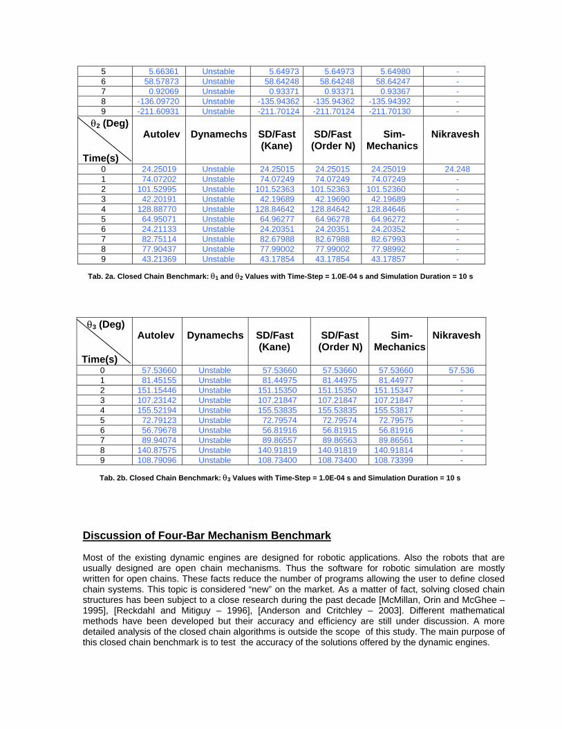
Tab. 2a. Closed Chain Benchmark: θ1 and θ2 Values with Time-Step = 1.0E-04 s and Simulation Duration = 10 s
Tab. 2b. Closed Chain Benchmark: θ3 Values with Time-Step = 1.0E-04 s and Simulation Duration = 10 s
Discussion of Four-Bar Mechanism Benchmark Most of the existing dynamic engines are designed for robotic applications. Also the robots that are usually designed are open chain mechanisms. Thus the software for robotic simulation are mostly written for open chains. These facts reduce the number of programs allowing the user to define closed chain systems. This topic is considered “new” on the market. As a matter of fact, solving closed chain structures has been subject to a close research during the past decade [McMillan, Orin and McGhee – 1995], [Reckdahl and Mitiguy – 1996], [Anderson and Critchley – 2003]. Different mathematical methods have been developed but their accuracy and efficiency are still under discussion. A more detailed analysis of the closed chain algorithms is outside the scope of this study. The main purpose of this closed chain benchmark is to test the accuracy of the solutions offered by the dynamic engines.

This test gives a negative point to Robotics Toolbox since this dynamic engine does not offer the closed chain option. Also the Nikravesh’s results (see tables 2a and 2b. - last column) included only three decimals. This lack of precision explains the difference in θ2(0) values. Also based on the values in tables 2a and 2b, we can conclude that Dynamechs appears to be limited as far as model definition is concerned. Indeed it appeared that increasing body mass without changing the inertia properties in an appropriate fashion could result in unstable simulations. This limitation has been confirmed by Dr. McMillan himself, who is the designer of this package. On the other hand, the mass values and inertia properties were fixed before starting any simulation and thus cannot be changed or adapted to suite any of the dynamic engines. Thus the model definition factor is considerably in favor of Autolev, SD/Fast and SimMechanics. These three dynamic engines are of the same order of accuracy within 0.1% of relative error, even though the accuracy of the different dynamic engines considered here is discussable. It is a certain fact that the four-bar model is a non-linear model and thus involves non-linear differential equations to solve. We know that the solver is the same in each case but the mathematical formulation is different. We can thus conclude that the different mathematical formulations used in this benchmark are equivalent and valid within the limits of our model. Also SD/Fast and SimMechanics values are much closer to each other compared to Autolev values. But this difference never exceeded 0.1% relatively. From a simulation point of view, SimMechanics, once again, has the most friendly-user interface. The rest of the dynamic engines are text-based as far as model definition and coding are concerned. A summary of the general features offered by each dynamic engine is presented in table 5 at the end of this document. Five-Bar Pendulum Benchmark Figure 3 shows a five-bar pendulum implemented to test the execution speed of the dynamic engines. The speed comparison can be found in tables 3a and 3b below. As mentioned before, a stopwatch was used and the average of 10 values was taken. The integration parameters are: Integration Time-Step = 1.0E-04 s
θ1
G
O Y
X
Simulation Duration = 10 s The following constants have been used throughout all simulations: G = 9.81 m/s2; Masses Mi = 1 kg for i = 1..5 (no inertia but masses located at center gravity, i.e. mid-bar); Lengths Li = 1 m for i = 1..5; θ1 (0) = 30 deg; Integration Time-step = 1.0E-04 s. Fig. 3. Five-Bar Pendulum This last comparison is presented in tables 3a and 3b below. As a reminder, the speed benchmark is significant only if the C/C++ based and Matlab based dynamic engines are separated into two distinct groups and compared to each other among each group.

Autolev Dynamechs4 SD/Fast (Kane) SD/Fast (Order N)Limited edition error 23.68 s 10.28 s 9.56 s
Robotics Toolbox SimMechanics 334.41 s 115.61 s
Discussion of Five-Bar Pendulum Benchmark Because of the memory restriction in the demo version of Autolev, the five-bar mechanism could not be run with this software. To provide a measure of execution speed for Autolev, we simulated the four-bar pendulum model with Autolev and other dynamic engines. The average execution times for 10 seconds of simulation were 5.04 s (Autolev), 23.68 s (Dynamechs), 15.77 s (SD/Fast Kane), 12.24 s (SD/Fast Order N) and 161.35 s (SimMechanics). In addition, the consistency of the model using θ1 time-history was verified. We can conclude that the user-friendly dynamic engines, especially SimMechanics, are much slower in execution than the other text based programs. In fact, graphical interfaces involve a lot of computational processing, making the software easy to use but slower too. Among this text-based group, Autolev is the fastest without loosing any accuracy as we observed previously. The disadvantage of Autolev being that it has its own language and coding generated by an executable. This would mean that during a global biomechanical simulation for instance, we would have to call Autolev externally and write a specific Autolev code for that model. This process might extend the simulation duration by non-negligible amount without counting the code generation itself. Summary and Conclusions In this study we compared several dynamic engines based on accuracy/precision and speed of execution. From the accuracy test, we deduce that all the different dynamic engines, besides Dynamechs and Robotics Toolbox, are equivalent within 0.01% of error. Dynamechs showed serious instability problems as soon as the body masses were increased without increasing the inertia properly. The other engines were not constrained from that point of view at all. Also Robotics Toolbox does not offer the closed chain option and thus had to be removed from this benchmark. For the speed of execution test, Autolev was revealed to be the fastest dynamic engine. The only disadvantage being that a specific Autolev code has to be generated every time that a mechanism needs to be assembled in order to define the generalized coordinates, reference frames and more. The other engines generate the dynamical parameters automatically. This factor is very important since it can save the user a considerable amount of time in pre- and post-processing. As expected, the order-N formulation of SD/Fast was verified to be faster than the Kane’s formulation. This difference in time increases when the system becomes more complex, i.e. includes loops or number of body N > 10. Robotics Toolbox offered very poor dynamical functions. Since this software is designed for robotic purposes only, the trajectories are usually imposed and the software generates the commands in order to follow the pre-defined patterns and calculate torques. Our main goal is to have a broader dynamic engine being able to provide both forward and backward dynamics without any restrictions. This package is thus not suitable to our purposes in the Matlab environment. The results of the accuracy and speed benchmarks along with other general features of the dynamic engines are summarized in table 4 on a one-to-ten based scale (1 = poor; 10 = excellent).
4 The inertial configuration (only) was changed in order to obtain a stable simulation. This duration value was added in order to measure the speed of Dynamechs for the same model (besides the inertial properties).
Tab. 3a. C/C++ Speed Benchmark: Integration Time-Step = 1.0E-04 s, Total Simulation Time = 10 s
Tab. 3b. Matlab Speed Benchmark: Time-Step = 1.0E-04 s and Total Simulation Time = 10 s

Table 4. Side-by-side comparison of Dynamic Engines
SD-Fast (Symbolic Dynamics Inc.)
Autolev (Dynamics Online)
SimMechanics (Mathworks Inc.)
Robotic Toolbox DynaMechs
Formulation Kane and proprietary order (N) Customized and simplified for
the specific model
Kane But facilitates implementing other formulation methods
Recursive order (N) Articulated Body Method
Recursive Newton-Euler – Walker and Orin. This is O (N3) but claims that for N<9 it is faster than Featherstone
Featherstone’s recursive order (N) Articulated Body method
Coordinate System Generalized coordinates Generalized Coordinates Relative coordinate Generalized coordinates Generalized/reduced coordinates
External Loads Yes – forces and torques are applied on bodies and joints via user-defined functions
Yes Yes – using a variety of actuators
Yes Yes
Constraints Both holonomic (position) and nonholonomic (velocity) constraints are handled
Tree joints – implicit in multibodyequations that are driven for DOF
only Closed-loop systems – breaks
into trees and loop joints, pro- vides assembly and initial velo- city analyses. Loop joints expli- citly enforced by Lagrange multi pliers Prescribed motion – explicitly
enforced by Lagrange multipliers
User constraints – user supplied constraints equations
Both holonomic (position) and nonholonomic (velocity) constraints are handled
Both position and velocity constraints are handled
Tree joints Closed-loop systems –
breaks into trees and loop joints, provides assembly and initial velocityanalyses. Loop joint cons- traints could be enforced in several ways Prescribed motion Constraints integrity
is enforced by Lagrange multipliers
Only tree joints are handled
Tree joints – implicit in multibody equations that are driven for DOF only Closed-loop systems –
added recently. Loop joints are modeled either as soft joints (stabilized by springs- dampers) or hard joints (stabilized by springs-dampers or Baumgarte method
System topology Open and Closed chains (10, Excellent benchmark results)
Grounded or free flying systems
Open and closed chains (7, Good benchmark results)
Open and closed chains (10, Excellent benchmark results)
Open loop systems (1, Poor/none benchmark results
Open and closed chains Fixed or mobile base (5, Average/unstable benchmark results)
Joint types Basic pin, slider, and ball joints
Plus pre-defined from basics, U, gimbal, bearing, free, bushing, cylinder, planar, and weld joints
Basic Revolute, Prismatic, ball, and weld joints
Plus many composites - combinations of the basic joints
Revolute and Prismatic.
Revolute (pin), Prismatic (slider), and ball joints
Body Types Rigid Rigid Rigid Rigid RigidCollision Detection No No No No Yes – hard and soft
contact Limitations Up to 300 bodies and 1000 DOF Different version differ on Some Simulink features Joints are limited to

Table 4. Side-by-side comparison of Dynamic Engines
SD-Fast (Symbolic Dynamics Inc.)
Autolev (Dynamics Online)
SimMechanics (Mathworks Inc.)
Robotic Toolbox DynaMechs
their allowable memory can not be used by SimMechanics blocks According to the documentation, block parameters could not be changed from Matlab command line but developers say it is possible. This is one way to export MSMS models
1-DOF revolute and prismatic joints found in robotics
Closed-chain systems are not handled
No prescribed motion
Additional utilities Kinematics data in any coordinate
Coordinate transformation (rotation matrix, quaternions, Euler angles)
Reaction forces at the joints Total system momentum,
kinetic energy, center of mass and inertia
Baumgarte stabilization of drifts in position and velocity constraints due to numerical integration
Facilitates implementing any dynamic formulation method
Equilibrium condition analysis
Solver for sets of nonlinear equations
Reaction forces and torques
Spline interpolation
Kinematic data using sensors
Reaction forces and torques
Steady-state analysis Assembly analysis
Useful function for robotic applications such as trajectory generation and Jacobian matrix
Support for MDH conventions
Extensive coordinate transformation functions
Forward/Inverse kinematics
Models of well-known robots: Puma 560 and Stanford Arm
Simulation of hydrodynamic forces
Simulation of contact forces
Numerical routines Explicit fixed and variable-step Runge-Kutta for non-stiff problems
Constrained linear least square solver
Constrained nonlinear root finder
Kutta-Merson numerical integration
Uses Simulink suite of stiff and non-stiff ODE solvers in tandem with constraint solvers. Simulink has no DAE solver, which has to be circumvented by SimMechanics.
Access to all numerical tools in Matlab and its toolboxes
Access to Matlab’s numerical utilities
Euler, Fixed and variable-step Runge-Kutta
Forward analysis Yes Yes Yes Yes YesInverse analysis Yes – Two ways:
Do forward simulation with all motion prescribed and read forces and torques
Yes – Uses inverse dynamics for open-loop and kinematic analysis for closed-loop topologies
Yes Yes
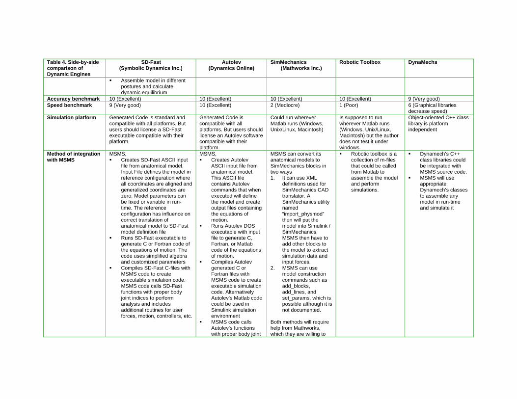
Table 4. Side-by-side comparison of Dynamic Engines
SD-Fast (Symbolic Dynamics Inc.)
Autolev (Dynamics Online)
SimMechanics (Mathworks Inc.)
Robotic Toolbox DynaMechs
Assemble model in different postures and calculate dynamic equilibrium
Accuracy benchmark 10 (Excellent) 10 (Excellent) 10 (Excellent) 10 (Excellent) 9 (Very good) Speed benchmark 9 (Very good) 10 (Excellent) 2 (Mediocre) 1 (Poor) 6 (Graphical libraries
decrease speed) Simulation platform Generated Code is standard and
compatible with all platforms. But users should license a SD-Fast executable compatible with their platform.
Generated Code is compatible with all platforms. But users should license an Autolev software compatible with their platform.
Could run wherever Matlab runs (Windows, Unix/Linux, Macintosh)
Is supposed to run wherever Matlab runs (Windows, Unix/Linux, Macintosh) but the author does not test it under windows
Object-oriented C++ class library is platform independent
Method of integration with MSMS
MSMS, Creates SD-Fast ASCII input
file from anatomical model. Input File defines the model in reference configuration where all coordinates are aligned and generalized coordinates are zero. Model parameters can be fixed or variable in run-time. The reference configuration has influence on correct translation of anatomical model to SD-Fast model definition file
Runs SD-Fast executable to generate C or Fortran code of the equations of motion. The code uses simplified algebra and customized parameters
Compiles SD-Fast C-files with MSMS code to create executable simulation code. MSMS code calls SD-Fast functions with proper body joint indices to perform analysis and includes additional routines for user forces, motion, controllers, etc.
MSMS, Creates Autolev
ASCII input file from anatomical model. This ASCII file contains Autolev commands that when executed will define the model and create output files containing the equations of motion.
Runs Autolev DOS executable with input file to generate C, Fortran, or Matlab code of the equations of motion.
Compiles Autolev generated C or Fortran files with MSMS code to create executable simulation code. Alternatively Autolev’s Matlab code could be used in Simulink simulation environment
MSMS code calls Autolev’s functions with proper body joint
MSMS can convert its anatomical models to SimMechanics blocks in two ways 1. It can use XML
definitions used for SimMechanics CAD translator. A SimMechanics utility named “import_physmod” then will put the model into Simulink / SimMechanics. MSMS then have to add other blocks to the model to extract simulation data and input forces.
2. MSMS can use model construction commands such as add_blocks, add_lines, and set_params, which is possible although it is not documented.
Both methods will require help from Mathworks, which they are willing to
Robotic toolbox is a collection of m-files that could be called from Matlab to assemble the model and perform simulations.
Dynamech’s C++ class libraries could be integrated with MSMS source code.
MSMS will use appropriate Dynamech’s classes to assemble any model in run-time and simulate it
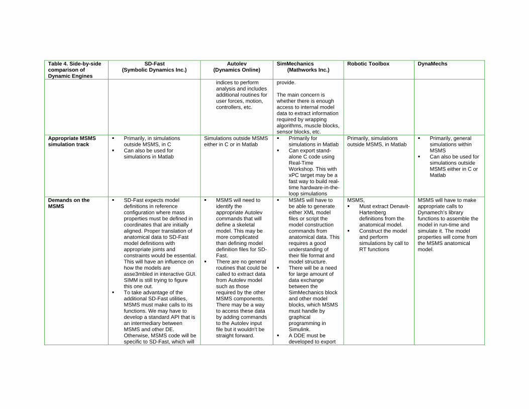
Table 4. Side-by-side comparison of Dynamic Engines
SD-Fast (Symbolic Dynamics Inc.)
Autolev (Dynamics Online)
SimMechanics (Mathworks Inc.)
Robotic Toolbox DynaMechs
indices to perform analysis and includes additional routines for user forces, motion, controllers, etc.
provide. The main concern is whether there is enough access to internal model data to extract information required by wrapping algorithms, muscle blocks, sensor blocks, etc.
Appropriate MSMS simulation track
Primarily, in simulations outside MSMS, in C
Can also be used for simulations in Matlab
Simulations outside MSMS either in C or in Matlab
Primarily for simulations in Matlab
Can export stand-alone C code using Real-Time Workshop. This with xPC target may be a fast way to build real-time hardware-in-the-loop simulations
Primarily, simulations outside MSMS, in Matlab
Primarily, general simulations within MSMS
Can also be used for simulations outside MSMS either in C or Matlab
Demands on the MSMS
SD-Fast expects model definitions in reference configuration where mass properties must be defined in coordinates that are initially aligned. Proper translation of anatomical data to SD-Fast model definitions with appropriate joints and constraints would be essential. This will have an influence on how the models are asse3mbled in interactive GUI. SIMM is still trying to figure this one out.
To take advantage of the additional SD-Fast utilities, MSMS must make calls to its functions. We may have to develop a standard API that is an intermediary between MSMS and other DE. Otherwise, MSMS code will be specific to SD-Fast, which will
MSMS will need to identify the appropriate Autolev commands that will define a skeletal model. This may be more complicated than defining model definition files for SD-Fast.
There are no general routines that could be called to extract data from Autolev model such as those required by the other MSMS components. There may be a way to access these data by adding commands to the Autolev input file but it wouldn’t be straight forward.
MSMS will have to be able to generate either XML model files or script the model construction commands from anatomical data. This requires a good understanding of their file format and model structure.
There will be a need for large amount of data exchange between the SimMechanics block and other model blocks, which MSMS must handle by graphical programming in Simulink.
A DDE must be developed to export
MSMS, Must extract Denavit-
Hartenberg definitions from the anatomical model.
Construct the model and perform simulations by call to RT functions
MSMS will have to make appropriate calls to Dynamech’s library functions to assemble the model in run-time and simulate it. The model properties will come from the MSMS anatomical model.

Table 4. Side-by-side comparison of Dynamic Engines
SD-Fast (Symbolic Dynamics Inc.)
Autolev (Dynamics Online)
SimMechanics (Mathworks Inc.)
Robotic Toolbox DynaMechs
make it difficult to switch to other DE. This is why SIMM is stuck with SD-Fast.
MSMS must do what a software package called XAL Package, http://www.concurrent-dynamics.com/xal/ does, i.e., Takes in the
anatomical model information and write the Autolev input program.
Invokes Autolev to compile input program to generate output C, Fortran, or Matlab files.
Modify the generated files so that it could be integrated with the rest of the simulation code easily.
the simulation outputs from SimMechanics model to MSMS animator.
Data exchange with MSMS and its components
Input data for muscles, sensor, other model components, and external hardware can be accessed by calls to SD-Fast utility functions.
SD-Fast’s user forces and user motion subroutines could apply force of muscles, other actuators, and external hardware.
MSMS must automatically generate the code to make calls to SD-Fast functions and generate subroutines for user forces and motion.
MSMS must be able to dynamically exchange data with the code compiled and run outside it to animate the motion in real-time. It should
Autolev has a specific input language, which might not facilitate the communication interface with MSMS
Variety of sensors and actuators could be used to exchange data between MSMS and SimMechanics. The number of lines connecting the SimMechanics and other MSMS blocks however could create a messy Simulink model
Data exchange could be done by calls to RT functions
Through calls to methods in class libraries.

Table 4. Side-by-side comparison of Dynamic Engines
SD-Fast (Symbolic Dynamics Inc.)
Autolev (Dynamics Online)
SimMechanics (Mathworks Inc.)
Robotic Toolbox DynaMechs
also read motion files after the simulation is completed.
Other third-party software requirements
Needs a C compiler to compile and link the MSMS and SD-Fast C-code
For C and Fortran files, requires a C or Fortran compiler For Matlab files, it will need Matlab to run
Requires Matlab and Simulink
Matlab None.
Added demand on the user
User may have to manually compile the MSMS and SD-Fast C-code, add his own code and possibly debug it. C programming knowledge is required
User may have to manually compile the MSMS and Autolev codes. Knowledge of Matlab is required for using Autolev’s Matlab code
The user must be familiar with Matlab and Simulink environment where the final model will run
Familiarity with Matlab None. The C++ libraries could be completely integrated with the MSMS executable
Access to source code and flexibility
The generated simulation C-code is accessible for inspection, modification, and debugging. The SD-Fast source code is however hidden from the user
The generated simulation code is accessible for inspection, modification, and debugging. The Autolev source code is however hidden from the user
The source code is not accessible but the graphical model in Simulink is accessible for high-level inspection, modification, and debugging
Matlab source code is accessible for manipulation.
The source code for the C++ class libraries are accessible for inspection, modification, and debugging
Documentation and Support
Good documentation with many examples Good technical support
Only a free tutorial available, all other documentations including the reference manual are commercial
Good documentation on the use of SimMechanic software. But integration of SimMechanics as dynamic engine in another software is neither considered nor documented. We will need Matlab’s help in this regard
User manual is good with tutorials and demos
C++ Classes are documented. There are example models with no documentation Developers invite feedback from users but no support could be expected. They have not responded to Peman’s email requests.
Developers and Distributors
Developed by Michael Sherman and Dan Rosenthal of Symbolic Dynamics Inc. Currently distributed by PTC
Online Dynamics Inc. Thomas Kane is in the board of directors.
Mathworks Inc. Peter Corke of CSIRO Manufacturing, Australia
Developed and distributed by Scott McMillan. Duane Marhefka has recently added closed-chain capabilities. Dynamechs is being gradually extended in Ohio State University.
Target applications and users
Simulation of general multibody systems. Used as engine for several commercial simulation packages
Symbolic manipulator for engineering and mathematics
Simulation of general mechanical systems
Kinematics and dynamics of serial-link robot manipulators
Started as part of a graduate project for dynamic and hydrodynamic simulation of under-water robots with star topologies.
Side-by-side parison of
ynamic Engines
SD-Fast (Symbolic Dynamics Inc.)
Autolev (Dynamics Online)
SimMechanics (Mathworks Inc.)
Robotic Toolbox DynaMechs
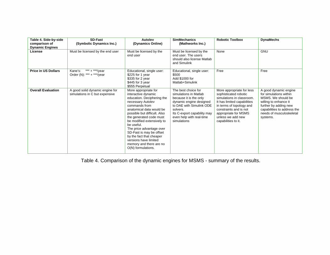
License Must be licensed by the end user Must be licensed by the end user
Must be licensed by the end user. The users should also license Matlab and Simulink
None GNU
Price in US Dollars Kane’s: *** + ***/year Order (N): *** + ***/year
Educational, single user: $225 for 1 year $335 for 2 year $445 for 3 year $555 Perpetual
Educational, single user: $500 Add $1000 for Matlab+Simulink
Free Free
Overall Evaluation A good solid dynamic engine for simulations in C but expensive
More appropriate for interactive dynamic education. Deciphering the necessary Autolev commands from anatomical data would be possible but difficult. Also the generated code must be modified extensively to be useful. The price advantage over SD-Fast is may be offset by the fact that cheaper versions have limited memory and there are no O(N) formulations.
The best choice for simulations in Matlab because it is the only dynamic engine designed to DAE with Simulink ODE solvers. Its C-export capability may even help with real-time simulations
More appropriate for less sophisticated robotic simulations in classroom. It has limited capabilities in terms of topology and constraints and is not appropriate for MSMS unless we add new capabilities to it.
A good dynamic engine for simulations within MSMS. We should be willing to enhance it further by adding new capabilities to address the needs of musculoskeletal systems.
Table 4. Comparison of the dynamic engines for MSMS - summary of the results.
Table 4.comD

References [Anderson and Critchley – 2003] Anderson K.S. and Critchley J.h., " Improved Order-n Performance Algorithm for the Simulation of Constrained Multi-Rigid-Body Systems", Multibody Systems Dynamics, Vol. 9, pp.185-212. [Betounes – 2001] Betounes D., “Differential Equations: Theory and Applications with Maple”, SBN 0-387-95140-7, English. [Corke – 2001] Corke P.I., “Robotics Toolbox for Matlab – Release 6” Queensland Center for Advanced Technologies, Copyright © 2000 QCAT. [Featherstone and Orin - 2000] Featherstone R. and Orin D.E., “Robotic Dynamics: Equations and Algorithms” IEEE Int. Conf. Robotics & Automation, pp. 826-834. [Hollars, Rosenthal and Sherman – 1994] Hollars M.G., Rosenthal D.E. and Sherman M.A., “SD/Fast User’s Manual Version B.2” Symbolic Dynamics, Inc. [Kane and Levinson – 1985] Kane T.R. and Levinson D.A., “Dynamics: Theory and Applications” McGraw-Hill, Inc. pp. 37-56 and 90-106. [McMillan – 1995] McMillan S., “Dynamechs Simulation Library: Reference Manual 3.0” DOC++ Roland Wunderling, Malte Zockler. [McMillan and Orin - 1995] McMillan S. and Orin D.E., "Efficient Computation of Articulated-Body Inertias Using Successive Axial Screws" IEEE Transactions on Robotics and Automation, August Edition, pp. 606-611. [McMillan, Orin and McGhee – 1995] McMillan S., Orin D.E. and McGhee R.B., “Underwater Robotic Vehicles: Design and Control” (J. Yuh, ed.) TSI Press, pp. 73-98. [McMillan, Orin and McGhee – 1995] McMillan S., Orin D.E. and McGhee R.B., “Efficient Dynamic Simulation of an Underwater Vehicle with a Robotic Manipulator” IEEE Transactions on Systems, Man, and Cybernetics, v.25, n.8, August Edition, pp. 1194 -1206. [McMillan, Orin and McGhee - 1996] McMillan S., Orin D.E. and McGhee R.B., "A Computational Framework for Simulation of Underwater Robotic Vehicle Systems," Special Issue of the Journal of Autonomous Robots on Autonomous Underwater Robots, vol. 3, pp. 253-268. [Nikravesh, 1988] Nikravesh, P.E., “Computer-Aided Analysis of Mechanical Systems” Prentice-Hall International, Inc. pp. 10-14, 135-137 and 268-270. [Reckdahl and Mitiguy – 1996] Reckdahl K.J. and Mitiguy P.C., “Autolev 3.0 Tutorial” Online Dynamics, Inc. [Wood and Kennedy – 2003] Wood G.D. and Kennedy D.C., “Simulating Mechanical Systems in Simulink with SimMechanics” The MathWorks, Inc.