APLICAÇÃO DO RISCO POTENCIAL DE FOGO DA ...
135
ALEX SANTOS DA SILVA APLICAÇÃO DO RISCO POTENCIAL DE FOGO DA VEGETAÇÃO EM ESCALA GLOBAL Tese apresentada à Universidade Federal de Viçosa, como parte das exigências do Programa de Pós-Graduação em Meteorologia Aplicada, para obtenção do título de Doctor Scientiae. VIÇOSA MINAS GERAIS – BRASIL 2019
-
Upload
khangminh22 -
Category
Documents
-
view
3 -
download
0
Transcript of APLICAÇÃO DO RISCO POTENCIAL DE FOGO DA ...

ALEX SANTOS DA SILVA
APLICAÇÃO DO RISCO POTENCIAL DE FOGO DA VEGETAÇÃO EM ESCALA GLOBAL
Tese apresentada à Universidade Federal de Viçosa, como parte das exigências do Programa de Pós-Graduação em Meteorologia Aplicada, para obtenção do título de Doctor Scientiae.
VIÇOSA MINAS GERAIS – BRASIL
2019

ALEX SANTOS DA SILVA
APLICAÇÃO DO RISCO POTENCIAL DE FOGO DA VEGETAÇÃO EM ESCALA GLOBAL
Tese apresentada à Universidade Federal de Viçosa, como parte das exigências do Programa de Pós-Graduação em Meteorologia Aplicada, para obtenção do título de Doctor Scientiae.
APROVADA: 24 de junho de 2019.

ii
Dedico, Ao Senhor Jesus Cristo, coroado de glória e de honra, que pela Graça de Deus, deu-me vida e vida com abundância. Aos meus amados pais: Florêncio e Imaculada.

iii
“Portanto, quer comais, quer bebais, ou façais outra coisa qualquer, fazei tudo para a glória de Deus.” Fonte: Bíblia Sagrada (1 Coríntios 10.31).

iv
SUMÁRIO
LISTA DE FIGURAS..........................................................................................
LISTA DE TABELAS.........................................................................................
RESUMO...........................................................................................................
ABSTRACT.......................................................................................................
CAPÍTULO 1.....................................................................................................
INTRODUÇÃO GERAL.....................................................................................
1.2 Objetivo Geral.............................................................................................
1.2.1 Objetivos específicos.........................................................................
1.3 Estrutura da Tese........................................................................................
CAPÍTULO 2......................................................................................................
ESTIMATIVAS DO RISCO DE FOGO EM VEGETAÇÃO.................................
2.1 Índice logarítmico de Telecyn......................................................................
2.2 Índice de Nesterov......................................................................................
2.3 Sistema de previsão de risco de incêndios florestais dos Estados Unidos.
2.4 Índice de tempo e incêndios florestais do Canadá......................................
CAPÍTULO 3......................................................................................................
DADOS UTILIZADOS E DESCRIÇÃO DO MODELO DE RISCO DE FOGO...
3.1 Reanálise e dados observados...................................................................
3.2 Índice de Risco Potencial de Fogo (PFI).....................................................
3.3 Índice de Risco Potencial de Fogo versão 2 (PFIv2)..................................
CAPÍTULO 4......................................................................................................
COMPARAÇÕES ENTRE AS ESTIMATIVAS DO PFI E DO PFIV2.................
4.1 Ocorrências de queimadas no período 2001-2016.....................................
4.2 Análises da variabilidade climática do PFI e do PFIv2................................
REFERÊNCIAS.................................................................................................
vii
xi
xii
xiii
1
1
4
4
5
5
5
6
7
9
11
15
15
15
16
20
24
24
25
28
34

v
CAPÍTULO 5......................................................................................................
ARTIGO SUBMETIDO......................................................................................
ABSTRACT.......................................................................................................
1. Introduction....................................................................................................
2. Data and Methodology..................................................................................
2.1 Study area...............................................................................................
2.2 Climate Data............................................................................................
2.3 Potential Weather Fire Index version 2 (PFIv2)......................................
2.4 Validation of the PFIv2 model.................................................................
3. Results and Discussion.................................................................................
3.1 Temporal variability of global fires...........................................................
3.2 Study of case analyses...........................................................................
3.2.1 July and August climatology in the 2001-2016 period…................
4. Case studies……….......................................................................................
4.1 August 1st to 15th, 2003 (SC01)……………….........................................
4.2 July 21st to 31st, 2018 (SC02)………………….........................................
5. The North Atlantic Oscillation (NAO) and the fire activity…….......................
6. Concluding Remarks.....................................................................................
7. Acknowledgements.......................................................................................
REFERENCES..................................................................................................
Tables................................................................................................................
Figures...............................................................................................................
CAPÍTULO 6......................................................................................................
ARTIGO PROPOSTO.......................................................................................
ABSTRACT.......................................................................................................
1. Introduction……………………………………………………….....…………….
2. Experimental design and model description…………………….……………..
40
40
41
42
44
44
45
45
49
49
49
56
56
58
58
59
61
62
63
63
71
71
86
86
87
88
91

vi
2.1. Potential Weather Fire Index version 2 (PFIv2)………………………….
3. Results and Discussion…………………………………………………………..
3.1. Sea surface temperature and precipitation variabilities………………....
3.2. Climatology in the 1998-2018 period………………………………………
3.3. The El Nino Southern Oscillation (ENSO) and the fire activity…………
4. Case studies………………………………………………………………………
4.1. Tropical fire risk and the La Nina 2011 (CS01)………………………..…
4.2. Tropical fire risk and the El Nino 2015 (CS02)………………………...…
4.3. Accumulated daily fire in the CS01 and CS02……………………………
5. Conclusions………………………………………………………………………..
6. Acknowledgements……………………………………………………………….
REFERENCES……………………………………………………………………….
Tables…………………………………………………………………………………
Figures………………………………………………………………………………...
CAPÍTULO 7………………………………………………………………………….
CONCLUSÕES E PERSPECTIVAS FUTURAS……………........………………
91
93
93
94
95
98
98
100
101
102
102
103
106
106
119
119

vii
LISTA DE FIGURAS
Figura 2.1. Fluxograma da estrutura do NFDRS. Os triângulos cinzas indicam as contribuições ponderadas das classes de combustíveis nos componentes de espalhamento e de energia liberada. Fonte: adaptado de Andrews e Bradshaw (1991)............................................................................ Figura 2.2. Estrutura do índice de tempo e incêndios do Canadá (FWI)......... Figura 3.1. Variação senoidal do Risco Básico RB em função dos dias de secura DS para sete classes de vegetação. Neste caso, sem precipitação, todos os fatores de precipitação assumem valor 1,0....................................... Figura 3.2. Função de crescimento logístico da variação total do IH. Apenas para a camada mais baixa do IH, altura inferior ou igual a 1.500 m................ Figura 4.1. Áreas de estudo. Fonte: adaptado da OMM................................. Figura 4.2. Sazonalidade das ocorrências de queimadas detectadas pelo satélite Terra/MODIS, de 2001 a 2016 para as seis áreas de estudo. Note: As escalas para a África (a)-(c) e América do Sul (g)-(i) são maiores............. Figura 4.3. Porcentagem do fogo diário acumulado na África, em cada classe do PFI e do PFIv2, durante o período 2001-2016. Note: O fator ZERO representa a relação total de focos de queimadas que foram detectados próximos ao valor zero de cada índice.......................................... Figura 4.4. Porcentagem do fogo diário acumulado na Ásia, em cada classe do PFI e do PFIv2, durante o período 2001-2016. Note: O fator ZERO representa a relação total de focos de queimadas que foram detectados próximos ao valor zero de cada índice............................................................. Figura 4.5. Porcentagem do fogo diário acumulado na América do Sul, em cada classe do PFI e do PFIv2, durante o período 2001-2016. Note: O fator ZERO representa a relação total de focos de queimadas que foram detectados próximos ao valor zero de cada índice.......................................... Figura 4.6. Porcentagem do fogo diário acumulado na América do Norte e Caribe, em cada classe do PFI e do PFIv2, durante o período 2001-2016. Note: O fator ZERO representa a relação total de focos de queimadas que foram detectados próximos ao valor zero de cada índice................................ Figura 4.7. Porcentagem do fogo diário acumulado no Pacífico Sudoeste, em cada classe do PFI e do PFIv2, durante o período 2001-2016. Note: O fator ZERO representa a relação total de focos de queimadas que foram detectados próximos ao valor zero de cada índice.......................................... Figura 4.8. Porcentagem do fogo diário acumulado na Europa, em cada classe do PFI e do PFIv2, durante o período 2001-2016. Note: O fator
10
13
19
23
25
28
29
30
31
32
33

viii
ZERO representa a relação total de focos de queimadas que foram detectados próximos ao valor zero de cada índice.......................................... Figure 5.1. (a) Study areas according to the WMO classification. (b) Vegetation distribution by IGBP (adapted from FRIEDL et al., 2010). (c) Temporal evolution of basic risk as function of the days of drought and vegetation……………....................................................................................... Figure 5.2. Flowchart presenting the sequence of calculation for the PFIv2.. Figure 5.3. Seasonality of fire occurrences detected by satellite Terra/MODIS from 2001 to 2016 for all six study areas. The trend equations are shown in the top right of each annual fire distribution. Note: The range values for Africa (a)-(c) and South America (g)-(i) are bigger than for another regions……………………………………………………………………………….. Figure 5.4. Anomalies in Precipitation (left side), and Basic Risk of fire (right side) for NDJF (a)-(b), MAMJ (c)-(d), JASO (e)-(f), and 2001-2016 period (g)-(h) by ERAInterim averages with respect to CPC averages for the period of 2001-2016. Black dots show statistically significant differences at 95%.................................................................................................................. Figure 5.5. Standard deviation of the Basic Risk by CPC data (left side), and anomalies between ERA-Interim and CPC averages (right side) for NDJF (a)-(b), MAMJ (c)-(d), JASO (e)-(f), and for all 2001-2016 period (g)-(h)……….……………………………………………………………………………. Figure 5.6. Present day (2001-2016) PFIv2 factors (a)-(c) for July-August-September-October (JASO), (d) is the PFIv2 based on ERAInterim climate data, on CPC global Precipitation, and on IGBP vegetation classes. Figures (e) and (f) are the annual trend and the standard deviation, respectively. Note. Figures (b) and (e) were multiplied by a hundred……………………….. Figure 5.7. Percentage of accumulated daily fire at each PFIv2 level based on ERAInterim, and CPC precipitation data for the 2001-2016 period. (a) Africa, (b) Asia, (c) South America, (d) Americas and Caribbean, (e) South-West Pacific and (f) Europe. ZERO indices are the percentage of fire events that were observed in a level closest to zero by PFIv2 (displayed in the top left corner of each panel)………………………………………………………….. Figure 5.8. Percentage of accumulated daily fire at each PFIv2 level in Europe for July (a) and; August (b) during the 2001-2016 period. ZERO indices are the percentage of fire events that were observed in a level closest to zero by PFIv2 (displayed in the top left corner of each panel)…….. Figure 5.9. July and August climatology in the 2001-2016 period. Maximum temperature at 2 m ((a), °C), relative humidity (b), surface pressure ((c), hPa), precipitation ((d), mm/day), PFIv2 factors (e)-(g) and, (h) PFIv2 over the accumulated fire event from 2003 (dots)……………………………………..
34
74
75
76
77
78
79
80
80
81

ix
Figure 5.10. Anomalies in (a) maximum temperature at 2 m (°C), (b) relative humidity (%), (c) surface pressure (hPa), (d) precipitation (mm/day), (e)-(g) PFIv2 factors, and (h) PFIv2 distribution for August 1st to 15th 2003 with respect to August averages for the period 2001-2016. Black dots on (h) denote local fires…………………………………………………………………… Figure 5.11. Anomalies in (a) maximum temperature at 2 m (°C), (b) relative humidity (%), (c) surface pressure (hPa), (d) precipitation (mm/day), (e)-(g) PFIv2 factors, and (h) PFIv2 distribution for July 21st to 31st 2018 with respect to July averages for the period 2001-2016. Black dots on (h) denote local fires……………………………………………………………………………. Figure 5.12. Correlation between Basic Risk and NAO for July (a) and August (b) in the 2001–2016 period. Correlation between PFIv2 and NAO for both months (c)-(d) at same period. Gridpoints that do not show statistically significant differences are shown in grey……………………………………..….. Figure 5.13. Correlation of individual and combined PFIv2 factors with NAO for SC01 (a)-(d) and SC02 (e)-(h). Gridpoints that do not show statistically significant differences are shown in grey…………………………………….…... Figure 6.1. (a) Study areas. (b) Vegetation distribution by IGBP (adapted from FRIEDL et al., 2010)…………………………………………………………. Figure 6.2. Flowchart presenting the sequence of calculation for the PFIv2... Figure 6.3. Annual series of the ONI from 1998 to 2018. Blue and red lines are the limit values for La Nina and El Nino respectively. Source:
OISST/NOAA………………………………………………………………………... Figure 6.4. Sea Surface Temperature (SST) climatology in the 1998-2018 period (a). (b) SST anomaly on La Nina events and; (c) SST anomaly on El Nino events. The black box shows the Nino3.4 region…………………………. Figure 6.5. Anomalies in CPC precipitation for El Nino (a); and La Nina (b) events in the 1998-2018 period. Black dots show statistically significant differences at 95%............................................................................................ Figure 6.6. Present day (1998-2018) climatology. Maximum temperature at 2 m ((a), °C), relative humidity (b), surface pressure ((c), hPa), precipitation ((d), mm/day), PFIv2 factors (e)-(g) and, (h) PFIv2…………………………….. Figure 6.7. PFIv2 factors on El Nino events during the 1998-2018 period (a)-(d). Figure (e) is the standard deviation. The same sequence is shown from (f)-(j), but for the difference between El Nino and La Nina events………. Figure 6.8. Percentage of accumulated daily fire at each PFIv2 for El Nino and La Nina events in (a) South America, (b) Africa, and (c) Australia in the 2001-2018 period. ZERO indices are the percentage of fire events that were observed in a level closest to zero by PFIv2 (displayed in the top left corner
82
83
84
85
109
109
110
110
111
112
113

x
of each panel)……………………………………………………………………….. Figure 6.9. Correlation between the PFIv2 and ENSO for El Nino (a), and La Nina (b) events in the 1998-2018 period. Gridpoints that do not show statistically significant differences are shown in grey…………………………… Figure 6.10. Sea Surface Temperature (SST) climatology in the 1998-2018 period (a). (b) SST anomaly on a La Nina event (2011) and; (c) SST anomaly on an El Nino event (2015)……………………………………………... Figure 6.11. Anomalies in (a) maximum temperature at 2 m (°C), (b) relative humidity (%), (c) surface pressure (hPa), (d) precipitation (mm/day), (e)-(g) PFIv2 factors, and (h) PFIv2 distribution for 2011 (La Nina event) with respect to climatology from 1998 to 2018………………………………………... Figure 6.12. Anomalies in (a) maximum temperature at 2 m (°C), (b) relative humidity (%), (c) surface pressure (hPa), (d) precipitation (mm/day), (e)-(g) PFIv2 factors, and (h) PFIv2 distribution for 2015 (El Nino event) with respect to climatology from 1998 to 2018………………………………………... Figure 6.13. Percentage of accumulated daily fire at each PFIv2 level in (a) South America; (b) Africa; and (c) Australia on La Nina (2011) and El Nino (2015) events. ZERO indices are the percentage of fire events that were observed in a level closest to zero by PFIv2 (displayed in the top left corner of each panel)………………………………………………………………………..
114 115
115
116
117
118

xi
LISTA DE TABELAS
TABELA 2.1. Grau de risco de fogo de Telicyn................................................ TABELA 2.2. Restrições na continuidade da somatória do Índice de Nesterov........................................................................................................... TABELA 2.3. Classes e graus de risco de incêndios de Nesterov................... TABELA 2.4. Classes, escala numérica e características do FWI................... TABELA 3.1. Valores da constante de inflamabilidade “A” e tipos de vegetação......................................................................................................... TABELA 3.2. Categorias do PFI....................................................................... TABELA 3.3. Cálculos dos termos A e B do Índice de Haines, conforme a elevação local................................................................................................... TABLE 5.1. Fire risk (PFIv2) levels.................................................................. TABLE 6.1. Fire risk (PFIv2) levels..................................................................
7
9
9
14
18
20
21 71
106

xii
RESUMO
SILVA, Alex Santos da, D.Sc., Universidade Federal de Viçosa, junho de 2019. Aplicação do risco potencial de fogo da vegetação em escala global. Orientador: Flávio Barbosa Justino. Coorientador: Alberto Waingort Setzer.
O fogo em vegetação tem um papel fundamental no sistema climático global.
Um passo importante para a redução de seus impactos é por meio de
investigação da suscetibilidade à ocorrência de queimadas em vegetação,
devido às condições atmosféricas. Portanto, o objetivo deste estudo é
aprimorar o Índice de Risco Potencial de Fogo, “PFI” (JUSTINO et al., 2010)
em escala global, particularmente nas regiões extratropicais. A nova versão do
índice (PFIv2) inclui uma função de crescimento logístico ajustada para as três
camadas atmosféricas do Índice de Haines (HAINES, 1988) e um fator de
ajuste da temperatura devido à variação da latitude. Em sua formulação, o risco
de fogo na vegetação aumenta com o aumento da duração de períodos secos,
tipo e ciclo natural da fenologia da vegetação, convecção e estabilidade da
atmosfera. Os dados atmosféricos da Reanálise ERA-Interim e de precipitação
do CPC/NOAA (Climate Prediction Center / National Oceanic and Atmospheric
Administration) foram aplicados como dados de entrada do modelo. As
validações das análises foram realizadas com o auxílio dos dados de fogo ativo
do satélite Terra do projeto MODIS/NASA (Moderate Resolution imaging
Spectrometer / Natonal Aeronautics and Space Administration). Em condições
atuais de tempo e da vegetação, o PFIv2 representou as principais áreas de
risco de fogo de ambos os hemisférios. Na região tropical, o PFIv2 apresentou,
em média, eficiência superior a 5% na detecção dos focos de queimadas, em
relação ao PFI. Já nas regiões extratropicais, essa diferença atinge valores de
até 15% nas principais classes dos índices. Nas avaliações da influência das
variabilidades climáticas El Niño Oscilação Sul e Oscilação do Atlântico Norte
no risco de fogo, correlações positivas e estatisticamente significativas a 95%
foram obtidas na América do Sul e Europa, respectivamente. A confiabilidade
do PFIv2 para a reprodução de áreas com alta atividade de fogo indica que
este índice é uma ferramenta útil para os tomadores de decisões, em previsões
de ocorrências globais de fogo em vegetação.
xiii
ABSTRACT
SILVA, Alex Santos da, D.Sc., Universidade Federal de Viçosa, June, 2019. Application of the potential risk of vegetation fire on a global scale. Adviser: Flávio Barbosa Justino. Co-adviser: Alberto Waingort Setzer.
Fire in vegetation plays a fundamental role in the global climate system. An
important step towards reducing its impacts is by investigating the susceptibility
to the occurrence of vegetation fires due to atmospheric conditions. Therefore,
this study aims to improve the Potential Fire Index, "PFI" (JUSTINO et al., 2010)
on a global scale, particularly in the extratropical regions. The new version of
the index (PFIv2) includes a logistic growth function adjusted for three
atmospheric layers from the Haines Index (HAINES, 1988) and a temperature
adjustment factor due to latitudinal variation. On its formulation, the fire risk in
vegetation increases with the increase in the duration of dry periods, type and
natural cycle of the phenology of vegetation, convection and stability of the
atmosphere. The atmospheric data of the ERA-Interim reanalysis and
precipitation of the Climate Prediction Center (CPC / NOAA) were applied as
input data of the model. The validations of the analyses were performed by the
active fire data of the Terra satellite from Moderate Resolution Imaging
Spectrometer / National Aeronautics and Space Administration (MODIS /
NASA) project. In current conditions of weather and vegetation, the PFIv2
represented the main areas of fire risk in both hemispheres. In the tropical
region, PFIv2 showed an average efficiency up to 5% in the detection of fire
occurrences in relation to the PFI. In the extratropical regions, this difference
reaches values of up to 15% over main classes of indices. In the evaluations of
the influence of the climatic variabilities El Niño South Oscillation and North
Atlantic Oscillation in the risk of fire, positive and statistically significant
correlations at 95% were obtained in South America and Europe, respectively.
The reliability of PFIv2 for the reproduction of areas with high fire activity
indicates that this index is a useful tool for decision makers, in forecasting
global fire occurrences in vegetation.

1
CAPÍTULO 1
INTRODUÇÃO GERAL
Um dos maiores responsáveis pelas mudanças climáticas é o incêndio
em vegetação (GIGLIO et al., 2013). Este atua como um condutor de
mudanças no ambiente natural. Impactos do fogo na vegetação são questões
proeminentes que envolvem mudanças do clima passado e futuro (LYNCH et
al., 2007; SCOTT, 2012).
De acordo com Laturner e Scherer (2004), na história evolutiva do
homem este utiliza o fogo desde as eras mais remotas, todavia, nas últimas
décadas cresceu a preocupação de vários setores da sociedade com o uso
indiscriminado do fogo. Embora destrutivo, o poder das queimadas pode ser
vital na saúde de alguns ecossistemas, ajudando a manter um equilíbrio entre
as muitas variedades de vida vegetal e animal.
Em condições florestais, o fogo limpa o solo e permite que a vegetação
restante prospere. Mantém a continuidade das pastagens, melhora os
nutrientes e retarda a introdução de espécies de plantas lenhosas (CARROL et
al., 2018). Em muitos ecossistemas, algumas espécies tornaram-se adaptadas
ao fogo, onde este pode se propagar e sobreviver.
No entanto, variações ocorreram com a advento da agricultura. O
homem passou a usar o fogo para limpar grandes extensões de terra para a
agricultura. Ao longo do tempo, o fogo de origem antrópica rompeu o delicado
equilíbrio nos ecossistemas tolerantes ao fogo e dizimou os ecossistemas que
não eram tolerantes. Segundo Collins e Stephens (2010), neste processo, a
vegetação apresenta quantidades crescentes de matéria orgânica disponíveis
para queimar quando o fogo retorna, criando conflagrações mais intensas e
mais destrutivas.
Associadamente, o efeito imediato da queima da vegetação é a
produção e liberação de gases, como o dióxido de carbono (CO2), monóxido de
carbono (CO), hidrocarbonetos e outros, que retornam para a atmosfera em
questão de horas. Em geral, estes gases são quimicamente ativos e interagem
com as hidroxilas (OH) presentes na atmosfera, alterando a eficiência da
oxidação e modificando a quantidade de ozônio troposférico (GALANTER et al.,
2000).

2
As queimadas possuem um papel significante no balanço de CO2 global
(TOSCA et al., 2013; LI et al., 2014). Os gases do efeito estufa, oriundos da
combustão nas vegetações intensificam o aquecimento da Terra e as
mudanças climáticas globais. Sazonalmente, os impactos das queimadas,
mesmo de intensidades equivalentes podem diferenciar-se amplamente
dependendo do período fenológico em que ocorrem. Em grande parte dos
trópicos, os incêndios predominantemente antrópicos, são geralmente limitados
à estação seca ou períodos de seca incomum (períodos de El Niño ou La Niña
nas mesmas regiões; HOFFMANN et al., 2009).
De acordo com o relatório da FAO “Fire Management – Global
Assessment 2006”, a quantidade de biomassa queimada anualmente
considerando todas as fontes é de cerca de 9,2 x 10⁹ toneladas. Incêndios
globais em vegetação consomem aproximadamente 5,1 x 10⁹ toneladas; 42 %
delas somente na África. Tais queimadas liberam cerca de 3,4 x 10⁹ toneladas
de CO2 e outras emissões. Contudo, há sequestro de carbono atmosférico para
a rebrota da biomassa vegetal e assim, em caso de desmate, o CO2 gerado
pelo incêndio contribui efetivamente para uma emissão líquida de carbono na
atmosfera.
Segundo Costa e colaboradores (2007), a queima de biomassa nos
ecossistemas devido à expansão da fronteira agrícola, à conversão de florestas
e cerrados em pastagens, e à renovação de cultivos agrícolas são alguns dos
mais importantes fatores que causam impactos sobre o clima e a
biodiversidade. As queimadas ainda provocam o empobrecimento do solo, a
destruição da vegetação, problemas de erosão e estão ligadas a alterações na
composição química da atmosfera (YORK et al., 2012).
Sabe-se que a ocorrência de fogo depende da quantidade, volume e
espaçamento dos materiais combustíveis no local, temperatura, velocidade e
direção do vento. Estes estão relacionados com a transmissão de calor
concomitante da condução, convecção e radiação (McRAE and SHARPLES,
2013). Contudo, existe um grande debate sobre a importância das forçantes
climáticas e antropogênicas na contribuição para ignição de incêndios em
vegetação. Nos extratrópicos, por exemplo, os incêndios representam o perigo
antrópico mais importante principalmente na região Euro-Mediterrânea (EU-
MED), onde uma média de 4,5 x 10³ km2 de áreas arborizadas e de mata

3
queimam anualmente (SAN-MIGUEL-AYANZ et al., 2013), causando
consideráveis danos econômicos, ambientais e perda de vida.
A principal causa do fogo natural procede das atividades de raios.
Globalmente, no entanto, a atividade humana é a que causa mais queimadas
(WHITLOCK, 2004). A taxa média de queimadas em gramíneas e savanas gira
em torno de 522,8 Mha ano-1, principalmente na África, Austrália, América do
Sul e sul da Ásia, enquanto que o remanescente ocorre em regiões florestais
da Terra (MOUILLOT and FIELD, 2005).
De fato, a distribuição e as propriedades ecológicas de muitos biomas do
mundo são afetadas significativamente pelos regimes de fogo (BOND et al.,
2005). Weisse e Goldman (2018) mostraram que as perdas anuais de florestas
verdes atingiram níveis de 29,7 x 10⁹ hectares em 2016. Todavia, o
desmatamento mostrou tendências de redução para o período compreendido
entre agosto de 2016 e julho de 2017, devido às áreas de preservação
ambiental e de planejamento ecológico.
Resumidamente, a ocorrência de incêndio na vegetação pode ser
descrita como qualquer atividade de fogo sobre a paisagem que consome
recursos naturais, independentemente da origem de ignição. Ele tem a
capacidade de causar danos significativos a um ecossistema ou pode ajudar a
mantê-lo, torná-lo mais resiliente. Contudo, o fogo florestal gerido é
amplamente determinado pelas condições em que o fogo existe e os resultados
esperados ou desejados dos esforços de gestão. Sistemas de classificação de
risco de fogo permitem a avaliação das condições ambientais que contribuem
para o perigo de incêndio (ou potencial) e distribuição do fogo (FOSBERG et
al., 1996; STOCKS et al., 1996; JUSTINO et al., 2013).
Avanços recentes na modelagem de circulação acoplada atmosfera-
oceano conduziram ao desenvolvimento de modelos numéricos de previsões
climáticas (DOBLAS-REYES et al., 2013). O potencial de tais sistemas de
previsão para informar aos tomadores de decisões, em diferentes setores
econômicos, é enorme devido à provisão de um grande número de variáveis
fisicamente consistentes, em uma escala temporal sub-diária de um a vários
meses de antecedência (MANZANAS et al., 2014). Em se tratando de
experimentos de sensibilidades, Whitlock et al. (2006) atribuíram às variações

4
do regime de fogo nos Andes argentinos o aumento interanual da variabilidade
climática e a intensificação do El Nino Oscilação Sul (ENOS).
Apesar de ainda relativamente escassos na literatura, alguns estudos de
modelagem foram conduzidos baseados no regime de fogo acoplado às
dinâmicas da vegetação (SCHEITER & HIGGINS, 2009; THONICKE et al.,
2010; JUSTINO et al., 2013). A maior parte deles usam muitos parâmetros
que incluem métodos avançados para os cálculos da interação entre as
características do solo, alocação de carbono, combustíveis e quantidade de
umidade na liteira. Devido à necessidade de vários parâmetros, estes
modelos complexos podem incluir também um nível considerável de
incertezas em simular a biomassa combustível e a competição entre as
plantas, o que levaria a uma falha na precisão entre os incêndios observados
e previstos (HICKLER et al., 2006).
Assim, propõe-se o aprimoramento do Índice de Risco Potencial de Fogo
(PFI) particularmente frente às regiões extratropicais. Essa é a segunda versão
do PFI (PFIv2), que também se enquadra entre os modelos de complexidade
intermediária. A calibração do PFIv2 foi regida pelos dados atmosféricos da
Reanálise ERA-Interim (DEE et al., 2011) e pelos dados de precipitação do
CPC (XIE et al., 2010). Já as validações, foram realizadas pelos focos de calor
do satélite Terra MODIS (Moderate Resolution Imaging Spectroradiometer) da
NASA (National Aeronautics and Space Administration).
1.2 Objetivo Geral
O objetivo geral da tese é aprimorar o Índice de Risco Potencial de
Fogo, “PFI” (JUSTINO et al., 2010) em escala global, particularmente nas
regiões extratropicais.
1.2.1 Objetivos específicos
Identificação e aplicação de novas variáveis com potencial de
melhora do desempenho do PFI;
Verificação do impacto do uso do tradicional Índice de Haines
implementado ao PFI;

5
Análise da variabilidade climática global em relação ao PFI;
Análise de acerto espacial do PFIv2 para as seis subregiões globais
da Organização Meteorológica Mundial;
Análise sazonal dos resultados do PFIv2.
1.3 Estrutura da Tese
Este trabalho é constituído de uma primeira parte, com introdução e
objetivos apresentados no capítulo 1; o capítulo 2 contém a revisão de
literatura sobre a dinâmica do clima, ocorrência do fogo na vegetação e seus
impactos. O capítulo 3 descreve os dados utilizados, o Índice de Risco
Potencial de Fogo (PFI) e, as modificações necessárias para melhoria do PFI
nas regiões extratropicais (PFIv2). Esta parte conclui com as referências
utilizadas em sua elaboração.
A segunda parte, que compõe os capítulos 4, 5 e 6 são os resultados,
em termos comparativos e de artigos para publicação em revistas científicas,
visando atender exigência do Programa de Pós-graduação em Meteorologia
Aplicada da UFV. Ambos os artigos estão estruturados em estilo convencional
para tais contextos: introdução, dados e metodologia, resultados e discussão,
conclusões, agradecimentos e referências.
A terceira e última parte é constituída pelo capitulo 7, que aborda as
conclusões e perspectivas do uso do PFIv2.
CAPÍTULO 2
ESTIMATIVAS DO RISCO DE FOGO EM VEGETAÇÃO
Um passo importante para a redução das queimadas é o uso da
modelagem na investigação da suscetibilidade da vegetação ao fogo. No
Hemisfério Norte, os Estados Unidos, Canadá e Rússia apresentam avanços
nos métodos desde o início da década de 70. Seus avanços decorrem a partir
das bases de temperatura e umidade relativa do ar a modelos complexos que
calculam interações entre as características do solo, alocação de carbono, e o
conteúdo de umidade na liteira (ARCHIBALD et al., 2009; BRADSTOCK, 2010).

6
Na América do Sul e Caribe, a equipe do Projeto Queimadas do
Instituto Nacional de Pesquisas Espaciais (INPE) desenvolveu, com base na
análise de ocorrência de centenas de queimadas, uma metodologia que
relaciona as condições atmosféricas (temperatura, umidade e precipitação) e
os tipos de vegetação na área de cada evento (SETZER et al., 2002).
Atualmente, seus produtos e documentação são livremente obtidos em
http://www.inpe.br/queimadas/portal/risco-de-fogo-meteorologia.
2.1 Índice logarítmico de Telicyn
Desenvolvido na União das Repúblicas Socialistas Soviéticas (URSS),
este índice tem como variáveis as temperaturas do ar e do ponto de orvalho,
ambas medidas às 13 horas. O índice é acumulativo, isto é: seu valor aumenta
gradativamente, como realmente acontece com as condições de risco a
incêndios, até que a ocorrência de uma chuva o reduza a zero, recomeçando
um ciclo de cálculos, conforme a equação 2.1.
n
iii rTI
1
log (eq. 2.1)
em que:
I = Índice de Telicyn;
r = temperatura do ponto de orvalho (°C);
T= temperatura do ar (°C);
log = logaritmo na base 10.
Neste índice, sempre que ocorrer uma precipitação igual ou superior a
2,5 mm, elimina-se a somatória e recomeça-se o cálculo no dia seguinte, ou
quando a chuva cessar. Na presença de precipitação, o índice é nulo. Quanto
ao grau de risco de fogo, o índice acumulativo apresenta 4 classes (Tabela
2.1).

7
TABELA 2.1. Grau do risco de fogo de Telicyn.
Valor de I Grau de Risco
2,0 Nenhum
2,1 a 3,5 Pequeno
3,6 a 5,0 Médio
> 5,0 Alto
2.2 Índice de Nesterov
O sistema de taxa de risco de fogo mais utilizado na Rússia é um
índice de ignição relativamente simples, denominado Índice de Nesterov (IN).
Ele fornece um índice geral de ignição potencial (FOSBERG et al., 1996;
STOCKS et al., 1996), baseia-se principalmente na inflamabilidade dos
combustíveis, e não na velocidade de propagação do fogo. As variáveis
atmosféricas para este índice são:
Temperatura do bulbo seco;
Temperatura do ponto de orvalho (extraída da umidade
relativa e temperatura);
Precipitação.
O índice é inicializado a zero e é determinado tomando-se a diferença
entre as temperaturas diárias do ar (bulbo seco) e do ponto de orvalho,
multiplica-se esta diferença pela temperatura do ar e então, cumulativamente
somam-se os valores sobre o número de dias, desde que a precipitação tenha
sido inferior a 3 mm. Na ocorrência de precipitação diária de 3 mm ou mais, o
índice retorna a zero (BUCHHOLZ e WEIDEMANN, 2000). Este índice é
expresso matematicamente por:
W
iiii TDTIN
1
(eq. 2.2)
onde:

8
IN = Índice de Nesterov;
W = número de dias com precipitação até 3 mm;
T = Temperatura (°C);
D = Temperatura do ponto de orvalho (°C).
Em dias com chuva, onde a precipitação pluviométrica é igual ou maior
a 3 mm, a inflamabilidade dos combustíveis se reduz substancialmente e o
valor de Ti – Di é quase nulo. Segundo Pyne e colaboradores (1996), o IN é
usado para agendar operações de queimadas diárias na Federação Russa.
Posteriormente, o IN foi aperfeiçoado na Polônia. Mantendo-se o padrão
acumulativo do índice, seu ajuste deu-se na consideração direta do DPV das
13 horas, mesmo horário das coletas da temperatura do ar (equação 2.3).
n
iii TDPVIN
1
(eq. 2.3)
sendo:
IN = Índice de Nesterov;
DPV = déficit de pressão de vapor do ar (milibares);
T = temperatura do ar (°C).
O DPV, por sua vez, é igual a diferença entre a pressão máxima de
vapor d’água e a pressão real de vapor d’água, sendo calculado neste caso,
pela equação 2.4.
100
1H
EDPV (eq. 2.4)
em que:
E = pressão máxima de vapor d’água (milibares);
H = umidade relativa do ar (%).
Na adaptação polonesa, a continuidade da somatória do Índice de
Nesterov é limitada pela ocorrência de uma série de restrições (Tabela 2.2).

9
TABELA 2.2. Restrições na continuidade da somatória do Índice de Nesterov.
Chuva (mm) Modificação no cálculo (diário)
2,0 Nenhuma.
2,1 a 5,0 Abater 50% no valor de IN calculado na véspera e somar IN do dia.
5,1 a 8,0 Abater 50% no valor de IN calculado na véspera e somar IN do dia.
8,1 a 10,0 Abandonar a somatória anterior e recomeçar o cálculo.
> 10,0 Quando a chuva cessar.
A Tabela 2.3 apresenta a variação do grau de risco deste índice,
mantidas as considerações originais.
TABELA 2.3. Classes e graus de risco de incêndios de Nesterov.
Classes de Perigo Valores de Nesterov Graus de Risco
I 300 Nulo
II 301 a 500 Pequeno
III 501 a 1000 Moderado
IV 1001 a 4000 Alto
V 4000 Extremo
2.3 Sistema de previsão de risco de incêndios florestais dos Estados
Unidos
O sistema nacional de previsão de risco de incêndios florestais dos
Estados Unidos (NFRDS) foi desenvolvido em 1972 e revisado em 1988, para
incluir respostas quanto às condições de seca, sensibilidade sazonal, materiais
combustíveis, condições do tempo e do clima (BURGAN, 1988). Os parâmetros
observados do tempo que conduzem a formulação do NFDRS são:
Temperatura do ar (F);
Umidade Relativa (%);
Cobertura de nuvem e tipo de precipitação;
Velocidade média do vento a 6 metros (mph);
Umidade do combustível;
Duração da precipitação (horas);

10
Quantidade de precipitação (polegadas);
Temperaturas mínima e máxima do ar (F);
Umidade relativa mínima e umidade relativa máxima (%).
No NFDRS, vinte modelos de combustíveis que representam os tipos
de vegetação e combustível são derivados usando-se uma combinação de
umidade do combustível morto (1 hora, 10 horas, 100 horas, e 1000 horas). O
teor de umidade de combustível vivo e quatro classes de tamanho de
combustível morto são calculados a partir dos dados meteorológicos e valores
de umidade. De modo que o combustível inoperante é determinado pelo
diâmetro da madeira ou do intervalo de queima. Vale destacar que a variável
de velocidade do vento influencia diretamente o componente de espalhamento,
mas não o de energia liberada (Figura 2.1).
Figura 2.1. Fluxograma da estrutura do NFDRS. Os triângulos cinzas indicam
as contribuições ponderadas das classes de combustíveis nos componentes de
espalhamento e de energia liberada. Fonte: adaptado de Andrews e Bradshaw
(1991).

11
Esse índice também possui os seguintes componentes de controle:
queimadas antrópicas (MCOI); ocorrência de queimadas devido às atividades
de raios (LOI) e; um índice de queima do material combustível por 0,3 m2 (FLI).
Uma descrição detalhada da evolução deste sistema de risco de fogo pode ser
obtido em Hardy e Hardy (2007).
2.4 Índice de tempo e incêndios florestais do Canadá
De acordo com Stocks e colaboradores (1989), este sistema consiste
de dois módulos: o índice de tempo e incêndios florestais canadenses (FWI,
em inglês) e o sistema de previsão da evolução do fogo (FBP, em inglês).
Possui um conjunto de tabelas que permitem estimar o perigo de incêndio
correspondente a cada um dos principais tipos de combustíveis, com base nas
observações de pluviosidade, umidade relativa do ar e velocidade do vento ao
meio dia local. Algumas dessas tabelas permitem introduzir correções
correspondentes a variações sazonais do estado da vegetação e da insolação.
Embora existam tabelas para cada um dos principais tipos de combustíveis, a
estrutura geral das tabelas para cada um dos principais tipos de combustíveis é
a mesma. Tabelas especiais permitem correções relativas a regiões
montanhosas, onde existem condições de grande secura, associadas à baixa
umidade relativa noturna.
O módulo FWI é utilizado no Canadá desde 1970 e consiste de seis
códigos detalhados de umidade e distribuição do fogo que contabilizam para
com os efeitos de umidade de combustível e vento na evolução do fogo em um
tipo de combustível padronizado (pinheiro maduro). Os componentes do
sistema FWI são obtidos diariamente, considerando-se os seguintes
parâmetros atmosféricos de entrada:
Temperatura do Bulbo seco;
Umidade Relativa (%);
Velocidade do Vento (10 m);
Precipitação acumulada (24 horas)

12
Os valores do índice apresentam uma relação direta com o grau de
perigo de incêndios. O FWI consiste de dez tabelas que são agrupadas em seis
blocos. Nos três primeiros blocos é analisado o efeito das condições
meteorológicas sobre o conteúdo de umidade dos vários tipos de combustíveis
orgânicos. Nos três últimos blocos são analisadas a quantidade de umidade
acumulada e as características do comportamento do incêndio. No que tange a
umidade, os componentes do FWI são:
Quantidade de umidade de combustível (FFMC): refere-se à
classificação numérica do conteúdo de umidade da camada
orgânica e dos combustíveis finos existentes na floresta; (passo de
tempo de 2/3 de um dia);
Quantidade de umidade de turfa (DMC): refere-se à classificação
numérica para a umidade média existente na camada orgânica não
compacta com 2 a 4 polegadas de profundidade (passo de tempo
de 12 dias);
Grau de secura (DC): refere-se à classificação numérica da
umidade média existente nas camadas orgânicas compactas e
profundas. Esta quantificação deve ser utilizada como um guia nas
atividades de supressão e preparação de longo prazo, em grandes
áreas (passo de tempo de 52 dias).
Em se tratando dos três últimos blocos, tem-se:
Índice de propagação inicial (ISI): refere-se à classificação numérica
da velocidade do incêndio (taxa de propagação), imediatamente
após a ignição, em um determinado tipo de material combustível;
Ajuste da quantidade de umidade da turfa (BUI): refere-se à
classificação numérica da quantidade de material combustível
disponível para a combustão. Esta quantificação é adequada para
uso como um guia nas atividades de preparação de curto prazo;
Índice meteorológico de incêndios (FWI): refere-se à classificação
numérica da intensidade potencial do incêndio em um determinado

13
tipo de combustível. Esta quantificação é um guia para as
atividades diárias de preparação e supressão.
O constituinte orgânico avalia a camada húmus na superfície da
floresta, que consiste da decomposição da liteira (folhas e outras vegetações
mortas) e do solo mineral. Combustível na superfície inclui árvores maiores do
que 2 metros; vegetação de gramíneas; liteira da superfície da floresta, e
material de madeira. Os três componentes de umidade adicionam umidade
para chuva e subtraem umidade para seca. Apesar dos três códigos possuírem
diferentes escalas de tempo, taxas, e quantidades de precipitação necessárias
para a saturação, qualquer um deles pode ser alto ou baixo em ralação aos
outros.
O FWI surge da combinação entre o ISI e o BUI (Figura 2.2), que
representa uma medida relativa da intensidade potencial de uma única
propagação do fogo com uma fonte de combustível padrão, no nível do terreno.
Cada um dos componentes do sistema FWI precisa ser examinado por uma
interpretação adequada dos efeitos das queimadas passadas e presentes na
inflamabilidade do combustível. Os componentes transmitem individualmente,
informações diretas sobre o fogo potencial florestal.
Observações ou previsões do tempo
Precipitação Umidade R. Temperatura
Vento
Vento
Precipitação Umidade Relativa
Temperatura
Precipitação Temperatura
Códigos de Umidade e combustíveis
FFMC
DMC
DC
Índices de propagação do fogo
ISI
BUI
FWI
Figura 2.2. Estrutura do Índice de tempo e incêndios do Canadá (FWI).
O FWI atua com uma escala numérica de intensidade do fogo e possui
as seguintes classes de risco: baixo, moderado, alto, muito alto e extremo

14
(Tabela 2.4). Ele combina o índice de propagação inicial e o índice de
crescimento do fogo. Paralelamente, o risco de fogo é um índice relativo de
quão fácil ocorre a ignição na vegetação, quão difícil o incêndio pode ser
controlado, e quantos danos a queimada pode causar.
TABELA 2.4. Classes, escala numérica e características do FWI.
Classes Escala Características
Baixo 0 a 5 Focos auto extintos; fraca ignição
Moderado 6 a 10 Queimadas superficiais; fácil controle
Alto 11 a 20 Fogo vigoroso em superfície
Muito Alto 21 a 30 Carece de suporte aéreo para a contenção
Extremo 30 Rápida propagação; controle improvável
Na última década, modelos conceituais que levam em conta o tipo do
ecossistema, e modelos de fogo baseados nas equações de balanço de
energia e combustível, incluindo físicas de combustão detalhadas e dados de
assimilação também foram empregados aos modelos de risco de fogo (MEYN
et al., 2007; MANDEL et al., 2008). Quase sempre, contudo, tais modelos
exigem um alto custo computacional. Semelhantemente, essa exigência seria
necessária no uso do FWI devido à quantidade de variáveis envolvidas, o que
também poderia gerar incertezas cumulativas. Já o IN, cuja dinâmica é mais
simples, falharia com pequenas variações espaciais.
Por isso, a motivação de se propor um aprimoramento do PFI com
características exponenciais, contínuas e orbitais, que também considere
limiares específicos do IH para as diferentes latitudes, inclusive nas regiões
extratropicais. A vantagem de utilizá-lo está no fato de se tratar de um modelo
de complexidade intermediária, que representa a suscetibilidade ao fogo com
variáveis atmosféricas e da vegetação acessíveis globalmente.

15
CAPÍTULO 3
DADOS UTILIZADOS E DESCRIÇÃO DO MODELO DE RISCO DE FOGO
3.1 Reanálise e dados observados
Dados de temperatura do ar e de umidade relativa da reanálise ERA-
Interim, de precipitação do Centro de Previsões Climáticas (CPC/NOAA),
classificação dos tipos de ocupação do solo do IGBP (International Geosphere-
Biosphere Programme) e produtos de fogo da sexta coleção de imagens
espectrômetras de resolução moderada do sensor Terra/MODIS foram
utilizados para calibrar e validar as simulações diárias do risco de fogo (2001-
2018):
(i) ERA-Interim (DEE et al., 2011), versão recente de reanálise
atmosférica produzida pelo Centro Europeu de Previsão do Tempo de meso-
escala (ECMWF, em inglês). A resolução espacial dos dados é a grade
Gaussiana reduzida N128, que é simétrica em torno do equador, com um
espaçamento aproximadamente uniforme na direção norte-sul, girando em
torno de 0,703° entre as latitudes. Contabilizam-se 128 pontos alinhados ao
longo do Meridiano de Greenwich, desde o equador até o polo em ambos os
hemisférios. Já o número de pontos na direção leste-oeste varia com a latitude,
com o espaçamento de grade uniforme de 0,703125° somente nas regiões dos
trópicos. Os dados e todos os detalhes intrínsecos estão disponíveis em
httpd://apps.ecmwf.int/datasets/data/interim-full-daily/levtype=pl/.
(ii) A resolução espacial do CPC (XIE et al., 2010) é de 0,5° de latitude e
longitude, na superfície da Terra. Essa análise inclui assimilação de dados
observados de precipitação diária, usando registros de aproximadamente
30.000 estações que são administradas por múltiplas agências. Registros
históricos, observações independentes de estações vizinhas, radares e
satélites, assim como previsões de modelos numéricos são aplicados no
controle de qualidade dos dados.

16
(iii) Classificação dos tipos de ocupação da terra do IGBP (CHANNAN et
al., 2014), dados reprojetados nas coordenadas geográficas de latitude e
longitude do sistema de referência EPSG: 4326. São espacialmente agregados
no período 2001-2012 em duas resoluções: 5’x5’ (1776 linhas x 4320 colunas;
aproximadamente 0,083°) e; 0,5° (296 linhas x 720 colunas). Detalhes e tabela
de classificação do método podem ser obtidos em http://glcf.umd.edu/data/lc/.
(iv) Terra / MODIS (Moderate Imaging Spectroradiometer) (GIGLIO et al.,
2016), produtos de fogo da sexta coleção de imagens espectrômetras de
satélite com resolução moderada. No processamento destes dados, incluem-se
algoritmos para eliminação de alarmes falsos, causados pelos desmatamentos
de pequenas florestas, precisão na detecção de incêndios de escala espacial
reduzida, ajuste quanto à presença de nebulosidade e rejeição expandida de
brilho do sol. Seus produtos são definidos em uma grade senoidal da Terra às
escalas espaciais de 250-m, 500-m, ou 1-km. Pelo fato das grades serem
grandes em sua totalidade (43.200 x 21.600 píxeis a 1 km, e 172.800 x 86.400
píxeis a 250 m), elas são divididas em células fixas de aproximadamente 10° x
10° de dimensões. A cada célula é atribuída uma coordenada horizontal e uma
coordenada vertical, variando de 0 a 35 e 0 a 17, respectivamente. A célula no
canto superior a esquerda (mais a noroeste) é numerada por (0,0). Fonte
disponível em https://earthdata.nasa.gov/earth-observation-data/near-real-
time/firms/active-fire-data.
Para a viabilização dos cálculos nas células de grade, um ajuste nos
dados de entrada do modelo (reanálise e vegetação) foi realizado através de
interpolação bilinear, alterando as resoluções espaciais para 1° de latitude e
longitude. As variáveis meteorológicas diárias utilizadas foram: precipitação,
temperatura do ar, temperatura do ponto de orvalho e umidade relativa.
3.2 Índice de Risco Potencial de Fogo (PFI)
O PFI foi desenvolvido internamente no Centro de Previsão do Tempo e
Estudos Climáticos (CPTEC), com base na análise de ocorrência de centenas
de queimadas nos principais biomas (tipos de vegetação) do Brasil, em função

17
das condições e históricos meteorológicos na área de cada evento (SETZER et
al., 2002). Toda a documentação do método está disponível no Portal do
Monitoramento de Queimadas e Incêndios do Instituto Nacional de Pesquisas
Espaciais (INPE), em http://www.inpe.br/queimadas.
O princípio do PFI é que quanto mais dias sem chuva, maior o risco de
queimada da vegetação; adicionalmente, são incluídos no cálculo o tipo e o
ciclo natural de desfolhamento da vegetação, temperatura máxima e umidade
relativa mínima do ar, assim como a presença do fogo na região de interesse.
A referência dos cálculos está nos “Dias de Secura” (DS), que é um número
hipotético de dias sem nenhuma precipitação durante os últimos 120 dias
(JUSTINO et al., 2010), respeitando as seguintes etapas:
1. Determina-se diariamente para a área geográfica de abrangência, o
valor da precipitação, em milímetros (mm), acumulada para onze
períodos imediatamente anteriores a 1; 2; 3; 4; 5; 6 a 10; 11 a 15; 16
a 30; 31 a 60; 61 a 90; e 91 a 120 dias.
2. Calculam-se os “fatores de precipitação” (FPs), cujos valores variam
de 0 a 1 para cada um dos 11 períodos, utilizando-se uma função
exponencial empírica de precipitação, em milímetros, para cada
período. As respectivas equações são:
FP1 = exp(-0,14Prec) (eq. 3.1)
FP2 = exp(-0,07Prec) (eq. 3.2)
FP3 = exp(-0,04Prec) (eq. 3.3)
FP4 = exp(-0,03Prec) (eq. 3.4)
FP5 = exp(-0,02Prec) (eq. 3.5)
FP6-10 = exp(-0,01Prec) (eq. 3.6)
FP11-15 = exp(-0,008Prec) (eq. 3.7)
FP16-30 = exp(-0,004Prec) (eq. 3.8)
FP31-60 = exp(-0,002Prec) (eq. 3.9)
FP61-90 = exp(-0,001Prec) (eq. 3.10)
FP91-120 = exp(-0,0007Prec) (eq. 3.11)
3. Calculam –se os “Dias de Secura” (DS):

18
DS = 105 x (FP1 x FP2 ... x FP61-90 X FP91-120) (eq. 3.12)
4. Determinar o risco de fogo potencial básico (RB) para cada um dos
tipos de vegetação considerada, usando a seguinte equação:
RBn-0,16 = 0,9 x (1 + sin(An-0,16 x DS)) / 2 (eq. 3.13)
A Tabela 3.1 mostra os dezessete tipos de vegetação do Programa
Internacional de Geosfera e Biosfera (CHANNAN et al., 2014) e suas
respectivas constantes de inflamabilidade “An-0,16”.
TABELA 3.1. Valores da constante de inflamabilidade “A” e tipos de vegetação.
Ordem Vegetação A
0 Porções de água * -x-
1 Florestas Contato; Campinarana 2
2 Ombrófila densa; alagados 1,5
3 Florestas Decíduas; Campinarana 2
4 Florestas Decíduas e sazonais 1,72
5 Florestas Mistas 2
6 Caatinga fechada 2,4
7 Savana; Caatinga aberta 3
8 Savana arbórea 2,4
9 Savana 3
10 Pastagens Gramíneas 6
11 Alagados permanentes 1,5
12 Agricultura e diversos 4
13 Áreas urbanas e construídas * -x-
14 Agricultura; vegetações naturais 4
15 Neve e gelo * -x-
16 Solos expostos e mineração * -x-
* valores indeterminados de A. Para estas classes, o RB é nulo.

19
A Figura 3.1 ilustra a variação do RB para os tipos de vegetação de
mesma constante A. O princípio básico deste método está no cálculo dos “dias
de secura”, que indica tanto um período real de dias sem chuva, como também
um período hipotético sem chuva calculado a partir da quantidade e distribuição
temporal das chuvas ocorridas. Resumindo, para um mesmo número de dias
sem chuva, uma pastagem terá o RB maior ao de uma floresta.
O RB tem valor máximo 0,9, e aumenta conforme uma curva senoidal ao
longo do tempo. Atribuiu-se a função senoidal devido à semelhança da
variação da intensidade e duração da luz solar ao longo do ano, adicionado a
fenologia da vegetação que naturalmente tende a seguir o mesmo ritmo.
Figura 3.1. Variação senoidal do Risco Básico RB em função dos dias de
secura DS para sete classes de vegetação. Neste caso, sem precipitação,
todos os fatores de precipitação assumem valor 1,0.
5. Dois outros fatores são considerados para o cálculo do índice de
risco de fogo potencial (PFI): a umidade relativa mínima (URmin) e a
temperatura máxima do ar (Tmax), ambas observadas às 18h UTC. O
risco aumenta (diminui) para URmin abaixo (acima) de 40% e Tmax
acima (abaixo) de 30° C.
PFI = RB x (a x URmin + b) x (c x Tmax + d) (eq. 3.14)
onde, as constantes valem: a = -0,006; b = 1,3; c = 0,02 e d = 0,4. A
Tabela 3.2 mostra as categorias para os níveis do PFI.

20
TABELA 3.2. Categorias do PFI.
Risco Mínimo Baixo Médio Alto Crítico
PFI < 0,15 0,15 < 0,4 0,4 < 0,7 0,7 < 0,95 ≥ 0,95
Vale destacar que as parametrizações propostas pelo PFI não
representam coerentemente a distribuição de risco de fogo potencial nas faixas
extratropicais, devido às diferenças dos padrões de precipitação e temperatura
entre a região equatorial e as demais latitudes (JUSTINO et al., 2013).
Portanto, faz-se necessário a inserção de conceitos compatíveis aos padrões
climáticos dos extratrópicos, que serão extraídos do Índice de Haines.
3.3 Índice de Risco Potencial de Fogo versão 2 (PFIv2)
O PFIv2 é uma busca de aprimoramento do PFI (JUSTINO et al., 2010).
Sua base é mantida, porém acrescentam-se o Índice de Haines (HAINES,
1988) acoplado a função de crescimento logístico e um fator de correção da
temperatura devido à variação da latitude, visando estimativas do risco de fogo
coerentes às observadas em regiões extratropicais, cujos limiares de
temperatura e umidade relativa do ar são totalmente distintas das faixas
equatorial e tropical. Vale mencionar que o PFIv2 é de complexidade
intermediária, pois preenche a lacuna entre os modelos mais simples e aqueles
extremamente complexos.
Os modelos mais simples usam somente temperatura e umidade relativa
para informar um índice relativo à condição inicial do fogo potencial (Índices de
Angstron, Nesterov e Telicyn). Já os mais complexos, como aqueles
desenvolvidos nos Estados Unidos e Canadá (National Fire-Danger Rating
System, NFRDS; Fire Weather Index, FWI; Fire Behavior Prediction System,
FBP) combinam medições de combustíveis, topografia, condições do tempo e
risco de ignição devido à contribuição antropogênica ou natural.
O Índice de Haines (IH) segue uma linha que combina dois fatores
atmosféricos importantes dentro de um modelo simplificado que razoavelmente
indica as áreas mais susceptíveis ao fogo, sendo extensivamente utilizado por
institutos de tempo e fogo nos Estados Unidos e Canadá. O IH estima a
severidade do incêndio na superfície da floresta baseado nas taxas de

21
variações verticais da temperatura e umidade (WINKLER et al., 2005;
POTTER, 2018). Seus cálculos dão-se pela combinação das três camadas da
atmosfera (Baixa, Média e Alta), somando-se os termos de estabilidade e
umidade do ar (Tabela 3.3).
TABELA 3.3. Cálculos dos termos A e B do Índice de Haines, conforme a
elevação local.
Elevação (m) Componente de estabilidade
(A)
Componente de umidade
(B)
Cálculos (hPa) Categorias Cálculos (hPa) Categorias Baixa
(≥ 1500) T950–T850 A=1 se < 4°C
A=2 se 4-7°C A=3 se ≥ 8°C
T850–Td850 B=1 se < 6°C B=2 se 6-9°C B=3 se ≥ 10°C
Média (1500 a 3500)
T850–T700 A=1 se < 6°C A=2 se 6-10°C A=3 se ≥ 11°C
T850–Td850 B=1 se < 6°C B=2 se 6-12°C B=3 se ≥ 13°C
Alta (≥ 3500)
T700–T500 A=1 se < 18°C A=2 se 18-21°C A=3 se ≥ 22°C
T700–Td700 B=1 se < 15°C B=2 se 15-20°C B=3 se ≥ 21°C
Os componentes A e B são então somados, e o resultado do IH varia de
2 (risco muito baixo de crescimento de fogo) a 6 (risco alto). Contudo, tais
limiares do IH serão redefinidos, em termos de temperatura do ar (JUSTINO et
al., 2010). Contudo, a aplicação isolada do IH é incompleta, devido à ausência
de uma base científica mais robustas (POTTER, 2018).
Por isso, em cada camada atmosférica do IH será aplicada a função de
crescimento logístico nos termos de estabilidade e umidade do ar. Esta função
considera um crescimento exponencial adicionado a uma capacidade limitante.
Sua avaliação dá-se quanto às suas características matemáticas e quanto ao
método de estimar seus parâmetros. A ideia da equação de crescimento
logístico foi adaptada daquela inicialmente utilizada para a representação do
crescimento animal e vegetal (SOUZA e FREITAS, 2014).
Sabe-se que as variáveis de umidade relativa mínima e de temperatura
máxima são inversamente proporcionais e geram mutuamente uma
contribuição exponencial para o crescimento da existência do fogo. Já a
capacidade limitante, é o valor que representa o limite máximo do somatório

22
dos parâmetros de estabilidade (A) e umidade (B) para cada camada
atmosférica do IH (Equação 3.15).
rii
iii eFKF
FKF
05,005,005,0
05,005,105,0
(eq. 3.15)
onde:
F0 é o valor mínimo do parâmetro de estabilidade (s) do IH;
r é a diferença entre o valor máximo do parâmetro de umidade (q) e o
valor mínimo do parâmetro de estabilidade (s) do IH, em cada camada da
atmosfera;
F é a conversão do IH em uma equação contínua (°C);
K é o fator limitante, que representa o valor máximo da soma de ambos
os parâmetros do IH (umidade e estabilidade da atmosfera). Vale mencionar,
que este cálculo também é para cada camada da atmosfera (Equação 3.16):
mese
qs
memse
qs
mese
qs
K
3500:
430,1
35001500:
365,1
1500:
362
maxmax
maxmax
maxmax
(eq. 3.16)
Neste caso, o sistema combina os parâmetros A e B de cada camada do
IH a um nível limitante, onde o crescimento da suscetibilidade ao fogo pela
atmosfera é retido, devido à umidade e à estabilidade vertical da atmosfera.

23
Assim, o crescimento exponencial diminui e eventualmente se nivela a um
estado de equilíbrio (Figura 3.2).
Figura 3.2. Função de crescimento logístico da variação total do IH. Apenas
para a camada mais baixa do IH, altura inferior ou igual a 1.500 m.
Em termos analíticos, a função de crescimento logístico (FL) do IH é
dada por:
mese
WWW
memse
WWW
mese
WWW
FL
3500:
89,1196,00067,0109
35001500:
53,0115,00056,0101
1500:
26,0072,00035,0107
235
234
235
(eq. 3.17)
Em que, W é a soma dos parâmetros de estabilidade e umidade do IH
(°C) e, o termo “e” é a elevação local (m).
Na sequência, um fator de correção da temperatura do ar, devido às
variações da latitude também é incluído (Equação 3.18):
24
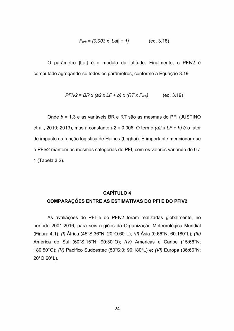
Forb = (0,003 x |Lat| + 1) (eq. 3.18)
O parâmetro |Lat| é o modulo da latitude. Finalmente, o PFIv2 é
computado agregando-se todos os parâmetros, conforme a Equação 3.19.
PFIv2 = BR x (a2 x LF + b) x (RT x Forb) (eq. 3.19)
Onde b = 1,3 e as variáveis BR e RT são as mesmas do PFI (JUSTINO
et al., 2010; 2013), mas a constante a2 = 0,006. O termo (a2 x LF + b) é o fator
de impacto da função logística de Haines (Loghai). É importante mencionar que
o PFIv2 mantém as mesmas categorias do PFI, com os valores variando de 0 a
1 (Tabela 3.2).
CAPÍTULO 4
COMPARAÇÕES ENTRE AS ESTIMATIVAS DO PFI E DO PFIV2
As avaliações do PFI e do PFIv2 foram realizadas globalmente, no
período 2001-2016, para seis regiões da Organização Meteorológica Mundial
(Figura 4.1): (I) África (45°S:36°N; 20°O:60°L); (II) Ásia (0:66°N; 60:180°L); (III)
América do Sul (60°S:15°N; 90:30°O); (IV) Americas e Caribe (15:66°N;
180:50°O); (V) Pacífico Sudoestec (50°S:0; 90:180°L) e; (VI) Europa (36:66°N;
20°O:60°L).

25
Figura 4.1. Áreas de estudo. Fonte: adaptado da OMM.
4.1 Ocorrências de queimadas no período 2001-2016
As ocorrências de queimadas detectadas pelo satélite Terra/MODIS
foram computadas e reclassificadas sazonalmente durante o período 2001-
2016 (Figura 4.2), para três diferentes intervalos: Novembro-Dezembro-
Janeiro-Fevereiro (NDJF); Março-Abril-Maio-Junho (MAMJ) e; Julho-Agosto-
Setembro-Outubro (JASO). Estes intervalos enfatizam as características
periódicas das ocorrências de incêndios interanuais, nos níveis mínimo,
intermediário e máximo.
Na Figura 4.2, pode-se observar que o período JASO apresenta as
maiores incidências de queimadas, em escala global. As Figuras 4.2(a)-(c)
mostram que as maiores ocorrências de queimadas são de julho a fevereiro na
África, com ocorrências superando 1 milhão de registros, em anos específicos.
Um período de transição é verificado no período MAMJ, com cerca de 300 mil
queimadas por ano, caracterizando-se como uma estação de poucos
incêndios. A alta atividade de queimadas na África (Figura 4.2c) é relacionada
às práticas de conversão da vegetação natural em pastagem e outros
propósitos agrícolas (SILVA et al., 2003).
As ocorrências de queimadas na Ásia são mostradas nas Figuras 4.2
(d)-(f). Durante o intervalo NDJF, os ventos no continente africano são
predominantemente de sul e a precipitação se desloca para a Ásia,
contribuindo com a redução e homogeneidade das queimadas (Figura 4.2d).
Quando a intensidade de radiação solar se eleva na Ásia (Figura 4.2e), os
ventos equatoriais tornam-se de norte e a monção asiática anula a atividade de

26
fogo. Adicionalmente, o sudoeste asiático é geralmente seco e quente, o que
também contribui para o aumento de ocorrências de queimadas (WOLFSON,
2012). No verão boreal, há uma redução nas atividades de fogo (Figura 4.2f),
devido à incidência dobrada na precipitação máxima, pelas áreas de monção
(SERREZE & BARRY, 2010).
Em relação à distribuição dos focos de queimadas na América do Sul,
as Figuras 4.2(g)-(h) mostram um padrão estável de novembro a junho, com
valores médios, girando em torno de 180 mil. Durante o período JASO (Figura
4.2i), a região central do Brasil experimenta condições extremas de seca.
Destaca-se também que os máximos valores de temperatura em superfície
ocorrem nos meses de Setembro e Outubro e a incidência de focos de
queimadas aumenta. A variabilidade interanual do fogo na América do Sul
responde a fase positiva (negativa) da Oscilação do El Niño (ENOS) tais como
em 2001, 2009 e 2014 (in 2005, 2007, 2008 e 2010). Estudos recentes
associam o aumento da ocorrência de queimadas às mudanças
antropogênicas da vegetação (SILVA et al., 2003; DAVIDSON et al., 2012;
SPERA et al., 2016).
De acordo com as Figuras 4.2(j)-(l), a incidência de fogo na América do
Norte e Caribe tende a ser estável de julho a fevereiro, quando as observações
máximas se aproximam de 100 mil queimadas, no período 2001-2016.
Recentemente, Van der Werf e colaboradores (2017) sugerem que as espécies
vegetativas da América do Norte possuem níveis intensos de combustíveis,
favorecendo as ocorrências de queimadas.
Na região do Pacífico Sudoeste (Figuras 4.2m-o), a baixa variação de
atividade de fogo ocorre no intervalo MAMJ (Figura 4.2n). Por outro lado,
variações interanuais são notórias nos períodos mais favoráveis ao fogo: NDJF
(Figura 4.2m) e JASO (Figure 4.2o). Estas variações se intensificam,
principalmente devido ao ciclo sazonal nas latitudes centrais da Austrália, que é
defasada por aproximadamente um ou dois meses daquelas localizadas nas
latitudes ao norte, cujos máximos ocorrem de novembro a janeiro, e os
mínimos de abril a junho. Nas regiões ao sul da Austrália, o ciclo sazonal é
atrasado em relação aos das latitudes centrais, com máximos geralmente de
dezembro a fevereiro e, mínimos de junho a agosto. De fato, estas diferenças

27
são associadas com os incêndios em vegetação que são raros em alguns
combustíveis, devido às características das plantas (CRUZ et al., 2018).
Embora as condições ambientais e dos atributos de vegetação sejam
relativamente similares na Europa e América do Norte (WOOSTER & ZHANG,
2004), as ocorrências de queimadas não são padronizadas, como mostrado
nas Figuras 4.2 (p)-(r). Destaca-se que apesar do aumento na ocorrência de
fogo em outubro e novembro, uma tendência negativa é observada no intervalo
JASO (Figura 4.2r).

28
Figura 4.2. Sazonalidade das ocorrências de queimadas detectadas pelo
satélite Terra/MODIS, de 2001 a 2016 para as seis áreas de estudo. Note: As
escalas para a África (a)-(c) e América do Sul (g)-(i) são maiores.
4.2 Análises da variabilidade climática do PFI e do PFIv2
O PFI e o PFIv2 foram avaliados pela eficiência na detecção de
ocorrências diárias de queimadas, nas classes máximas (entre 0,7 e 1) do risco

29
de fogo. As Figuras 4.3 a 4.8 apresentam, sequencialmente, as mesmas
regiões e intervalos da Figura 4.2. Entretanto, uma avaliação anual para o
período de 2001 a 2016 é adicionada.
Como visto anteriormente, a África é o continente com as maiores
ocorrências de queimadas. As Figuras 4.3(a)-(c) mostram que ambos os
índices detectam a variabilidade sazonal nas classes máximas (alto e crítico).
No intervalo JASO (Figura 4.3a), a eficiência foi de 93,5% (93%) para o PFIv2
(PFI). A similaridade dos índices permaneceu, proporcionalmente ao número
total de queimadas 88,7% (88,2%), no período NDJF (Figura 4.3b). Todavia, a
Figura 4.3(c) mostra que no intervalo de menor atividade de fogo na África
(MAMJ), a eficiência do PFIv2 superou em 0,7% a do PFI. Já na avaliação
anual (Figura 4.3d), a porcentagem do número total de focos detectados nas
classes máximas forai de 88,4% (87,9%) pelo PFIv2 (PFI).
Figura 4.3. Porcentagem do fogo diário acumulado na África, em cada classe
do PFI e do PFIv2, durante o período 2001-2016. Note: O fator ZERO
representa a relação total de focos de queimadas que foram detectados
próximos ao valor zero de cada índice.

30
Entre as regiões analisadas, a Ásia foi a que apresentou a menor
variabilidade entre as classes dos índices. Isso ocorre porque a amplitude
sazonal da ocorrência de queimadas é alta na Ásia, na qual as observações
diferem-se em aproximadamente 400 mil observações entre os intervalos NDJF
e MAMJ (Figuras 4.2d-e). Apesar disso, mais de 63% dos focos foram
detectados sazonalmente pelas classes máximas do PFIv2 (Figuras 4.4a-c). No
que tange à eficiência anual dos índices (Figura 4.4d), o PFI detectou 52,8%
das atividades de fogo, enquanto que o PFIv2 cravou 63% nas classes
máximas.
Figura 4.4. Porcentagem do fogo diário acumulado na Ásia, em cada classe do
PFI e do PFIv2, durante o período 2001-2016. Note: O fator ZERO representa a
relação total de focos de queimadas que foram detectados próximos ao valor
zero de cada índice.
A América do Sul também é caracterizada com valores similares aos
de detecção nas classes máximas dos índices (Figuras 4.5a-d). Porém a
eficiência do PFIv2 é maior, em média 1%, do que a do PFI, como mostrado no
intervalo JASO (Figura 4.5a).

31
É importante mencionar que a América do Sul é a região que
apresentou a maior taxa de ocorrências de queimadas na classe mínima
(Figura 4.5b). Isso se explica não somente pela variação sazonal, mas também
pelo conjunto de dados de precipitação, que tem sido constantemente
aprimorado para as latitudes tropicais e, pelo efeito antrópico nos avanços de
fronteiras agrícolas. As eficiências no intervalo MAMJ e anuais (Figuras 4.5c-d)
foram de 63,3% (61,9%) e 71,4% (70,4) para o PFIv2 (PFI).
Figura 4.5. Porcentagem do fogo diário acumulado na América do Sul, em
cada classe do PFI e do PFIv2, durante o período 2001-2016. Note: O fator
ZERO representa a relação total de focos de queimadas que foram detectados
próximos ao valor zero de cada índice.
As modificações nos parâmetros do PFIv2 para as latitudes
extratropicais demonstram a eficiência do método em detectar as ocorrências
de queimadas nas respectivas regiões. Na América do Norte e Caribe (Figuras
4.6a-d), as diferenças em relação ao PFI são de 5% e 3% nos intervalos JASO
(Figura 4.6a) e MAMJ (Figura 4.6c), respectivamente.
Na eficiência anual, os valores são de 60,8% para o PFI e de 64,8%
para o PFIv2. Estes resultados sugerem que o intervalo NDJF foi fundamental

32
para equilibrar as eficiências, ou seja: melhores ajustes ainda são necessários
para os intervalos de baixas ocorrências de queimadas.
Figura 4.6. Porcentagem do fogo diário acumulado na América do Norte e
Caribe, em cada classe do PFI e do PFIv2, durante o período 2001-2016. Note:
O fator ZERO representa a relação total de focos de queimadas que foram
detectados próximos ao valor zero de cada índice.
Em relação a região do Pacífico Sudoeste, que registra uma média de
150 mil ocorrências de queimadas no período 2001-2016 (Figures 4.2m-o), há
uma eficiência superior a 74% nos intervalos JASO e NDJF, cujas atividades
do fogo são máximas na região (Figuras 4.7a, b). As diferenças em relação ao
PFI nestes intervalos são de 2,3% e 1,7%, respectivamente.
Entretanto, a maior diferença entre as eficiências dos índices pode ser
observada no intervalo MAMJ (Figura 4.7c), cujo valor do PFIv2 (PFI) é 66,8%
(60,8%). Na avaliação anual (Figura 4.7d), o PFIv2 mostra que o nível de
acerto nas classes máximas é de 74,3%, enquanto que o PFI atinge 71,7%.
Vale mencionar que a porcentagem dos focos que ocorrem nos níveis próximos
a zero dos índices são iguais a 3,5%, o que pode ser considerado baixo, em se
tratando de acumulados diários, para o período de 2001 a 2016.

33
Figura 4.7. Porcentagem do fogo diário acumulado no Pacífico Sudoeste, em
cada classe do PFI e do PFIv2, durante o período 2001-2016. Note: O fator
ZERO representa a relação total de focos de queimadas que foram detectados
próximos ao valor zero de cada índice.
As análises na Europa revelam os efeitos do aprimoramento do PFIv2,
em todos os intervalos analisados. Pode-se observar que as diferenças nas
eficiências máximas foram de 6% (Figura 4.8a) a incríveis 20,3% (Figura 4.8c).
Contudo, um alerta é acionado: a necessidade de ajustes para os intervalos de
ocorrências mínimas de fogo (Figura 4.8b). No intervalo NDJF, por exemplo, a
razão dos focos detectados em áreas próximas a nulidade dos índices foi a
máxima (39,3%) entre todas as 6 regiões.
Apesar dessa discrepância, a eficiência anual do PFIv2 na Europa está
acima de 66,5%, representando uma diferença de 11,1%, em relação ao PFI.
Esta identificação é de suma importância no entendimento de que ambos os
índices indicam a suscetibilidade atmosférica ao fogo em vegetação, não
separando sistematicamente as parcelas de contribuições antrópicas e
naturais.

34
Assim, o próximo capítulo discutirá, o aprimoramento e a aplicação do
PFIv2 nas análises climáticas e de estudos de casos na Europa. Este estudo
visará a redução dos desafios encontrados pelos tomadores de decisões, na
previsão da atividade de fogo em vegetação.
Figura 4.8. Porcentagem do fogo diário acumulado na Europa, em cada classe
do PFI e do PFIv2, durante o período 2001-2016. Note: O fator ZERO
representa a relação total de focos de queimadas que foram detectados
próximos ao valor zero de cada índice.
REFERÊNCIAS
ARCHIBALD, S.; ROY, D. P.; VAN WILGEN, B. W.; and SCHOLES, R. J. What limits fire? An examination of drivers of burnt area in Southern Africa. Global Change Biology, v. 15, p. 613– 630, 2009.
ANDREWS, P. L.; and BRADSHAW, L. S. Use of meteorological
information for fire management in the United States. In ‘Workshop on Meteorological Information for Fire Management in the United States’, pp. 325-332, 1991.

35
BOND, W. J.; WOODWARD, F. I.; and MIDGLEY, G. F. The global distribution of ecosystems in a world without fire. New Phytologist, v. 165, p. 525-537, doi: 10.1111/j.1469-8137.2004.01252.x, 2005.
BRADSTOCK, R. A. A biogeographic model of fire regimes in Australia:
current and future implications. Global Ecology and Biogeography, 19, 145-158. doi: 10.1111/j.1466-8238.2009.00512.x, 2010.
BUCHHOLZ, G.; and WEIDEMANN, D. The Use of Simple Fire Danger Rating Systems as a Tool for Early Warning in Forestry. Int. Forest Fire News, v. 23, p. 32–37. www.fire.unifreiburg.de/iffn/country/id/id_29.htm, 2000.
BURGAN, R. E. Revisions to the 1978 National Fire-Danger-Rating System.
USDA Forest Service, Southeastern Forest Experiment Station Research Paper SE-273. (Asheville, NC), 1988.
CARROL, A.; VAN PELT, R.; and SILLET, S. C. Tree-Ring Indicators of
Fire in Two Old-Growth Coast Redwood Forests. Fire Ecology, v. 14, p. 85-105, doi: 10.4996/fireecology.140185105, 2018.
CHANNAN, S.; COLLINS, K.; and EMANUEL, W. R. Global mosaics of the
standard MODIS land cover type data. University of Maryland and the Pacific Northwest National Laboratory, College Park, Maryland, USA, 2014.
COLLINS, B. M.; and STEPHENS, S. L. Stand-replacing patches within a
‘mixed severity’ fire regime: quantitative characterization using recent fires in a long-established natural fire area. Landscape Ecology, v. 25, p. 927-939, doi: 10.1007/s10980-010-9470-5, 2010.
COSTA, M. H.; YANAGI, SILVIA, N. M.; SOUZA, P. J. O. P.; RIBEIRO, A.;
ROCHA, E. J. P. Climate change in Amazonia caused by soybean cropland expansion, as compared to caused by pastureland expansion. Geophysical Research Letters, Vol. 34, p. L07706, 2007.
CRUZ, M. G.; GOULD, J. S.; HOLLIS, J. J.; and McCAW, W. L. A
Hierarchical Classification of Wildland Fire Fuels for Australian Vegetation Types. Fire, 1, 13; doi:10.3390/fire1010013, 2018.
DAVIDSON, E. A.; de ARAÚJO, A. C.; ARTAXO, P.; BALC, J. K.; BROWN,
l. F. et al. The amazona basin in transition. Nature, v. 481, n. 7381, p. 321-328, 2012.
DEE, D. P.; UPPALA, S. M.; SIMMONS, A. J.; BERRISFORD, P.; POLI, P.;
et al. The ERA-Interim reanalysis: Configuration and performance of the data assimilation system. Quarterly Journal of the Royal Meteorological Society, v. 137(656), p. 553-597, 2011.

36
DOBLAS-REYES, F. J.; GARCÍA-SERRANO, J.; LIENERT, F.; BIESCAS, A. P.; RODRIGUES, L. R. L. Seasonal climate predictability and forecasting: status and prospects. Wiley Interdisciplinary Rev.: Climate Change, Vol. 4, p. 245-268, 2013.
FAO. Fire management global assessment. A thematic study prepared in
the framework of the Global Forest Resources Assesment. Food and Agriculture Organization of the United Nations, 2006.
FOSBERG, M.A.; STOCKS, B.J.; and LYNHAM, T.J. Risk analysis in
strategic planning: fire and climate change in the boreal forest. Fire in Ecosystems of Boreal Eurasia. J.G. Goldammer and V.V. Furyaev, editors. Kluwer Academic Publication, Netherlands, p. 495-504, 1996.
GALANTER, M.; LEVY II, H.; and CARMICHAEL, G. R. Impacts of biomass
burning on tropospheric CO, NOx and O3. Journal of Geophysical Research, Vol. 105, n. D5, p. 6633-6653, 2000.
GIGLIO, L.; RANDERSON, J. T.; and VAN DER WERF, G. R. Analysis of
daily, monthly, and annual burned area using the fourth-generation global fire emissions database (GFED4). Journal of Geophysical Research: Biogeosciences, v. 118, p. 317-328, doi: 10.1002/jgrg.20042, 2013.
GIGLIO, L.; SCHROEDER, W.; JUSTICE, C. O. The collection 6 MODIS
active fire detection algorithm and fire products. Remote Sensing of Environment, v. 178, p. 31-41, 2016.
HAINES, D. A. A lower atmospheric severity index for wildlands fires.
National Weather Digest, v. 13, p. 23-27, 1988. HARDY, C. C.; and HARDY, C. E. Fire danger rating in the United States of
America: an evolution since 1916. International Journal of Wildland Fire, v. 16, p. 217-231, 2007.
HICKLER, T. et al. Implementing Plant Hydraulic Architecture within the LPJ
Dynamic Global Vegetation Model. Global Ecology and Biogeography, v. 15, No. 6, pp. 567-577, 2006.
HOFFMANN, A. A.; PARRY, J.; CUAMBE, C.; KWESHA, D.; ZHAKATA, W.
Climate change and wildland fires in Mozambique. In M. A. Cochrane (Ed.), Tropical Fire Ecology: Climate Change, Land Use, and Ecosystem Dynamics. Springer/Praxis, Heidelberg, Germany/Chichester, U.K., 2009.
JUSTINO, F.; de MELO, A. S.; SETZER, A.; SISMANOGLU, R.;
SEDIYAMA, G. C.; RIBEIRO, G. A.; MACHADO, J. P.; STERL, A. Greenhouse gas induced changes in the fire risk in Brazil in ECHAM5/MPI-OM coupled climate model, Climatic Changes, Vol. 106, p. 285-302, 2010.

37
JUSTINO, F.; PELTIER, W. R.; BARBOSA, H. A. Atmospheric susceptibility to wildfire occurrence during the Last Glacial Maximum and mid-Holocene. Palaeogeography, Palaeoclimatology, Palaeoecology. Vol. 295, p. 76-88, 2010.
JUSTINO, F.; STORDAL, F.; CLEMENT, A.; COPPOLA, E.; SETZER, A.;
and BRUMATTI, D. Modelling Weather and Climate Related Fire Risk in Africa. American Journal of Climate Change, v. 2, p. 209-224, 2013.
LATURNER, N.; SCHERER, H. W. As queimadas e os incêndios florestais
em Mato Grosso. Revista Geonotas, Vol. 8, 2004. LI, F.; BOND-LAMBERTY, B.; and LEVIS, S. Quantifying the role of fire in
the Earth system – Part 2: Impact on the net carbon balance of global terrestrial ecosystems for the 20th century. Bigeosciences, 11, 1345-1360, doi: 10.5194/bg-11-1345-2014, 2014.
LYNCH, A. H.; BERINGER, J.; KERSHAW, P.; MARSHALL, A.; MOONEY,
S.; TAPPER, N.; TURNEY, C.; KARRS, S. V. D. Using the Paleorecord to Evaluate Climate and Fire Interactions in Australia, Annual Review of Earth and Planetary Sciences, Vol. 35: 215-239, 2007.
MANDEL, J et al. A wildland fire model with data assimilation. Mathematics
and Computers in Simulation. Vol. 79, p. 584-606, 2008. MANZANAS, R.; FRÍAS, M. D.; CONFIÑO, A. S.; GUTIÉRREZ, J. M.
Validation of 40 year multimodel seasonal precipitation forecasts: the role of ENSO on the global skill. Journal of Geophysical Research: Atmospheres, v. 119, p. 1708-1719, 2014.
McRAE, R. H. D.; and SHARPLES, J. J. A process model for forecasting
conditions conducive to blow-up fire events. Proceedings, MODSIM Conference, Adelaide, SA, 2013.
MEYN, A.; WHITE, P. S.; BUHK, C.; JENTSCH, A. Environmental drivers of
large, infrequent wildfires: the emerging conceptual model. Progress in Physical Geography. Vol. 31, p. 287-312, 2007.
MOUILLOT, F.; and FIELD, C. B. Fire history and the global carbon budget:
a 1° x 1° fire history reconstruction for the 20th century. Global Change Biology, 11, 398 – 420. doi: 10.1111/J.1365-2486.2005.00920.X, 2005.
POTTER, B. The Haines Index – it’s time to revise it or replace it.
International Journal of Wildland Fire, 27(7), p. 437-440 [https://doi.org/10.1071/WF18015], 2018.
PYNE, S. J.; ANDREWS, P. L.; and LAVEN, R.D. Introduction to Wildland
Fire. John Wiley & Sons, Inc., New York, NY, 769 p., 1996.

38
SAN-MIGUEL-AYANZ, J.; MORENO, J. M.; and CAMIA, A. Analysis of large fires in European Mediterranean landscapes: Lessons learned and perspectives. Forest Ecology and Management, v. 294, p. 11-22, 2013.
SCHEITER, S.; and HIGGINS, S. I. Impacts of Climate Change on the
Vegetation of Africa: An Adaptive Dynamic Vegetation Modeling Approach, Global Change Biology. Vol. 15, No. 9, p. 2224-2246, 2009.
SCOTT, J. H. Introduction to Wildfire Behavior Modeling. National
Interagency Fuels, Fire & Vegetation Technology Transfer. Available: www.niftt.gov, 2012.
SERREZE, M. C.; and BARRY, R. G. Climate change. In: BARRY, R. G.,
CHORLEY, R. J. (Eds.), Atmosphere. Weather and Climate. Routledge, Oxon, 2010.
SETZER, A.; SISMANOGLU, R. A. Queimadas no Brasil. Climanálise
Boletim de Monitoramento e Análise Climática, v. 7, n. 8, p. 40-53, 2002. SILVA, J. M. N.; PEREIRA, J. M. C.; CABRAL, A. I.; VASCONCELOS, M. J.
P.; MOTA, B.; and GREGOIRE, J. M. An Estimate of the Area Burned in Southern Africa during the 2000 Dry Season Using SPOT-VEGETATION Satellite Data. Journal of Geophysical Research, v. 108, No. D13, 2003.
SOUZA, L. A.; and FREITAS, C. E. C. Modelos populacionais de
ecossistemas. Revista Agrogeoambiental. v. 6, No. 3, 2014. SPERA, S. A.; GALFORD, G. L.; COE, M. T.; MACEDO, M. N.; and
MUSTARD, J. F. Land-Use Change Affects Water Recycling in Brazil's Last Agricultural Frontier. Global Change Biology, doi:10.1111/gcb.13298, 2016.
STOCKS, B.J.; LAWSON, B.D.; ALEXANDER, M.E.; VAN WAGNER, C.E.;
MCALPINE, R.S.; LYNHAM, T.J.; and DUBÉ, D.E. The Canadian Forest Fire Danger Rating System: an overview [reprinted from August 1989 issue, 65:258-265, with corrections and new pagination]. Forestry Chronicle, 65(6), p. 450-457, 1989.
STOCKS, B.J.; and LAWSON, B.D. El sistema Canadiense de evaluacion
del grado de peligro de incendios forestales: Una vision general. p. 82-94 in J.A. Guillermo, Editor. Proc. Prognosis Y Gestion en Control de Incendios Forestales, Actas del Taller Internacional, November 8-10, 1995, Santiago de Chile. Proyecto FONDEF FI-13, Santiago de Chile, 1996.
THONICKE, K; SPESSA, A; PRENTICE, I. C.; HARRISON, S. P.; DONG,
L.; and CARMONA-MORENO, C. The Influence of Vegetation, Fire Spread and Fire Behaviour on Biomass Burning and Trace Gas Emissions: Results from a Process-Based Model. Biogeosciences Discussions, V. 7, No. 1, pp. 697-743, 2010.

39
TOSCA, M. G.; RANDERSON, J. T.; and ZENDER, C. S. Global impact of smoke aerosols from landscape fires on climate and the Hadley circulation. Atmospheric Chemistry and Physics, v. 13, p. 5227-5241, doi: 10.5194/acp-13-5227-2013, 2013.
VAN DER WERF, G. R.; RANDERSON, J. T.; GIGLIO, L. et al. Global fire
emissions estimates during 1997-2016. Earth System Science Data, v. 9, p. 697-720, https://doi.org/10.5194/essd-9-697-2017, 2017.
WEISSE, M.; and GOLDMAN, L. 2017 Was the Second-Worst Year on
Record for Tropical Tree Cover Loss. Global Forest Watch. Online available at [https://blog.globalforestwatch.org/data-and-research/2017-foi-o-segundo-pior-ano-ja-registrado-de-perda-de-cobertura-florestal-tropical], 2018.
WINKLER, J. A et al. A climatology of the Haines Index for North America derived from NCEP/NCAR reanalysis fields. Sixth Fire and Forest Meteorology Symposium, American Meteorological Society, 2005.
WHITLOCK, C.; and BARTLEIN, P. J. Holocene fire activity as a record of
past environmental change, in: Developments in Quaternary Science, edited by: Gillespie, A. R., Porter, S. C., and Atwater, B. F., Elsevier, Amsterdam, 2004.
WHITLOCK, C.; MORENO, P. I.; and BARTLEIN, P. Climatic controls of
Holocene fire patterns in southern South America, Quaternary Research, v. 68, p. 28–36, 2006.
WOLFSON, R. Energy, Environment and Climate, second ed. WW Norton
and Company Inc, New York, pp. 366-370, 2012. WOOSTER, M. J.; and ZHANG, Y. H. Boreal forest fires burn less intensely
in Russia than in North America. Geophysical Research Letters, v. 31, n. L20505, https://doi.org/10.1029/2004GL020805, 2004.
XIE, P.; CHEN, M.; and SHI, W. CPC unified gauge analysis of global daily
precipitation. Preprints, 24th Conference on Hydrology. Atlanta, Georgia. American Meteorological Society, 2.3A. [Avaiable online at https://ams.confex.com/ams/90annual/webprogram/Paper163676.html], 2010.
YORK, A.; BELL, T. L.; and WESTON, C. J. Fire regimes and soil-based
ecological processes: implications for biodiversity. In Bradstock R. A et al (Eds) ‘Flammable Australia, Fire regimes, biodiversity and ecosystems in a changing world’ (CSIRO Publishing: Collingwood, VIC), p. 127-148, 2012.

40
CAPÍTULO 5
ARTIGO SUBMETIDO
IMPROVEMENT OF THE POTENTIAL WEATHER FIRE INDEX ON A
GLOBAL PERSPECTIVE
A. Silva
Agricultural Engineering Department, Federal University of Vicosa, Brazil.
F. Justino
Agricultural Engineering Department, Federal University of Vicosa, Brazil.
A. Setzer
Fire Program of the National Institute of Space Research (INPE), Brazil.
A. Avila
Agricultural Engineering Department, Federal University of Vicosa, Brazil.

41
ABSTRACT
On a global perspective, fire activities have been significantly linked to multiple
factors such as climate conditions, population density, agriculture, and
substantial economic losses. Based on vegetation susceptibility to fire, this
study presents the Potential Weather Fire Index version 2 (PFIv2). Here we use
ERA-Interim Reanalysis and CPC Unified Precipitation as input data for the
2001-2016 period. It has to be noticed that the PFIv2 estimates the risk by
considering local factors such as latitude, and topography profile. We
demonstrate that PFIv2 has revealed an efficiency by up to 70% in presenting
observed fires from Terra/MODIS satellite, over extratropical regions, mainly in
North America, Europe, and Asia. To evaluate in further details the PFIv2
performance, two extreme fire occurrences in Europe are considered. The first
event occurred in Portugal in 2003 (SC01), and the second in Greece in 2018
(SC02). In the SC01 event, the PFIv2 increases by up to 30%, over the highest
fire concentration in Western Europe, between 40°N and 55°N, related to the
direct influence of atmospheric instability, lower relative humidity, and
precipitation deficit. During the SC02 event, there is an increase (decrease)
variation of air temperature, over northern Europe (Balkan Peninsula), and dry
conditions are dominant over most part of Europe. The PFIv2 reveals accuracy
in reproducing the regions with fire activity in northern Central Europe, and
southwestern Russia. Further analyzes indicate that there is no correlation
between the North Atlantic Oscillation Index (NAO) and the PFIv2 with the
highest fire occurrences in the SC01. Conversely, a positive correlation
(statistically significant at 95%), between the NAO and the PFIv2 in the SC02
points that the atmospheric pattern linked to the NAO has the potential to
increase the fire risk. These findings indicate that the PFIv2 is an useful tool for
decision makers, in forecasting fire activity.
Keywords: Fire risk, vegetation, extratropical, atmospheric conditions,
logarithmic function.

42
1. Introduction
Climate and wildfire interaction plays a dynamic role as disturbance
agents affecting the structure and composition of flammable ecosystems
(HOLLMANN et al., 2013). In recent decades, various sectors of society have
expressed concern over the indiscriminate use of wildfire because vegetation
wildfires are prominent in issues involving past and future climate change (e.g.
HARRISON et al., 2007). Nevertheless, there is a lively debate on the
importance of anthropogenic and climate forcing in contributing to the ignition of
wildfires (HUANG et al., 2015).
Although the majority of vegetation wildfires has been observed in the
tropics, the Arctic and the extra-tropics have experienced in recent decades an
increased number of wildfires (VERAVERBEKE et al., 2017; MASRUR et al.,
2018). These regions have been affected by increased temperature and have
experienced distinct pattern of precipitation that can result in more vulnerable
conditions for wildfire development (KRAUSE et al., 2014; VERAVERBEKE et
al., 2017). In fact, there is a lack of studies on the interaction between climate
changes and expansion or suppression of fire seasons on a global perspective.
Thus, more investigation is necessary to disentangle the interchange between
anthropogenic factors and the natural environmental changes.
Historical fire evidences suggest that the onset of industrialization and
demand for land and timber, impose threat to forest cover in large parts of
Europe, Central/South America, China and India (GFRA, 2015). Extreme erratic
fires have been occurred leading to social disruptions and substantial economic
losses. The National Iteragency Fire Center (NIFC, 2013) has shown that over
the last decade, annual wildfire suppression costs on US federal lands
exceeded $1.7 billion US dollars. While in Canada this values reached by up to
$1 billion US dollars (GONZÁLEZ-CABÁN, 2013). Thus, the understanding and
skill to predict wildfire occurrence and intensity is essential to designing and
implementing necessary measures to mitigate these impacts.
In addition to the destructive power, burning in vegetation releases
carbon dioxide (CO2), carbon monoxide (CO), methane (CH4), hydrocarbons
and others, which return to the atmosphere in a matter of hours (GALANTER et
al., 2000). Fires present a significant role in the global CO2 balance, mainly over

43
an ecosystem restoring that suffered with fires. In this process, CO2 is gradually
removed from the atmosphere by photosynthesis and it is incorporated into the
reconstructed vegetation (TOSCA et al., 2013; LI et al., 2014). Greenhouse
gases originating from combustion in vegetation begin to intensify the global
warming. According to the FAO report “Fire Management – Global Assessment
2006”, the amount of biomass burned annually from all sources is about 9.2
billion tons. Global fires in vegetation consume 5.13 billion tons, 42% only in
Africa. Such fires release about 3.4 billion tons of CO2 and other emissions.
Modelling the fire activity is vital. The state-of-art fire modelling uses
several parameters that include complex methods to calculate the interaction
among soil characteristics, carbon allocation, and the moisture content of soil
litter (CATCHPOLE, 2002; ARCHIBALD et al., 2009; BRADSTOCK, 2010).
However, these models may also present a considerable uncertainty level on
parameterizing biomass fuel amount, which leads to a lack of accuracy between
predicted and observed fires (HICKLER et al., 2006; WARMINK et al., 2010;
FINNEY et al., 2012; SKINNER et al., 2014).
Van Wagner (1987) proposed the Fire Weather Index (FWI), which
currently is a worldwide index. It combines three moisture indices: the Fine Fuel
Moisture Code (FFMC) representing the moisture content in fine fuels. In
addition, the Duff Moisture Code (DMC) shows loosely compacted organic
material, while the Drought Code (DC) is a deep layer of compact organic
material. The combination of these moisture parameters delivers the fire
behavior indexes. Due to nonlinearity with respect to control effort, a power
function for daily Severity Rating (DSR) is implemented to increase the weight
of higher values of the FWI (VAN WAGNER 1970; WILLIAMS, 1959).
Similarly, the United States National Fire Danger Rating System
(NFDRS) was revised with the addition of Keetch-Byram Drought Index (KBDI),
to account for weather and climatic conditions in the eastern United States
(BURGAN, 1988). There are eleven weather parameters that drive the various
models of the NFDRS. In the NFDRS, 20 fuel models representing the
vegetation and fuel types can be selected, ranging from annual grass and herbs
to Alaskan tundra (ANDREWS and BRADSHAW, 1997). These fuel models are
derived by using a combination of dead fuel moisture (1-hour, 10-hour, 100-
hour, and 1000-hour) and live moisture (wood and grass) models (Burgan,

44
1988). The moisture content of live fuel and the four classes of dead fuel are
calculated from weather data and moisture values (RICHARD and HEIM 2002).
In summary, dead fuel is determined by the diameter of the wood or timelag.
Currently, the lightning ignition efficiency algorithm is being used by the United
States Wild Land Fire Assessment System (SOPKO et al., 2016).
Thus, the large number of degree of freedom arises criticism towards the
need to include several parameters for simulating the link between fire and
ecosystem dynamics (SCHEITER & HIGGINS, 2009). The Potential Weather
Fire Index (PFI), presented by Justino et al (2010) to predict regions in Brazil
more favorable to wildfires, formulated a simplified index based on four
parameters to calculate the fire risk. The modification on the PFI proposed here
replace the one level humidity factor by a logistic growth function, which inserts
three atmospheric layers and the local altitude as addressed on Haines Index
(1988). Afterwards, a correction factor of the air temperature due to latitudinal
change is included.
The goal of this study is to introduce and validate a modified version of
the Potential Weather Fire Index (JUSTINO et al., 2010), particularly on
extratropical regions. Section 2 describes the vegetation and climate data
utilized, the modelling formulation, and the validation methods. Section 3
discusses the capability of the PFIv2 in reproducing two cases of erratic fires in
Portugal and Greece in 2003 and 2018, respectively. Concluding remarks and
model limitation are described in Section 4.
2. Data and Methodology
2.1. Study area
The PFIv2, a modified version of the Potential Fire Index (PFI) proposed
by Justino et al (2010) is applied globally (Figure 5.1a), over six subdivisions
from World Meteorological Organization (WMO): (I) Africa (45°S:36°N;
20°W:60°E); (II) Asia (0:66°N; 60:180°E); (III) South America (60°S:15°N;
90:30°W); (IV) Americas and Caribbean (15:66°N; 180:50°W); (V) South-West
Pacific (50°S:0; 90:180°E) and; (VI) Europe (36:66°N; 20°W:60°E). Information
on the types of vegetation required for the computation of PFIv2 were obtained

45
from the classification of the International Geosphere-Biosphere Programme
(IGBP), as shown in Figure 5.1(b).
2.2. Climate Data
The calculation of the second version of the Potential Weather Fire Index
(PFIv2) is conducted based on the ERA-Interim Reanalysis (DEE at al., 2011),
and on the CPC Unified Precipitation Project that is underway at NOAA Climate
Prediction Center (Xie et al., 2010) for the 2001-2016 period. The spatial
resolution of the ERA-Interim Reanalysis (ERAI) is the reduced Gaussian grid
N128, which is symmetrical around the equator, with an approximately uniform
spacing in the north-south direction, spinning around 0.703125° between the
latitudes. There are 128 points aligned along the Greenwich Meridian, from the
equator to the pole in both hemispheres. The number of points in the east-west
direction varies with latitude, with uniform grid spacing of 0.703125° only in the
regions of the tropics.
The CPC spatial resolution is 0.5° latitude and longitude grid over global
land areas. This gauge-based analysis of daily precipitation uses reports from
over 30,000 stations that are collected from multiple agencies. Historical
records, independent information from measurements at nearby stations, radar
and satellite observations, as well as numerical model forecasts are applied in
the quality control of the data.
2.3. Potential Weather Fire Index version 2 (PFIv2)
The Potential Weather Fire Index version 2 (PFIv2) represents an
improvement of an earlier version proposed by Justino et al (2010). The main
assumption is maintained, but the PFIv2 includes a modified Haines Index
(HAINES, 1988) embedded to a logistic growth function, and a temperature
correction factor due to latitudinal variation to capture the wildfire risk estimates
consistent with those observed in extratropical regions.
The PFIv2 is highly correlated with the duration of the dry periods, the
type and natural cycle of defoliation of the vegetation, maximum temperature

46
and the humidity of the air. The reference of the calculations is the “Days of
Dryness” (DD), which is a hypothetical number of days without precipitation
during the last 120 days (JUSTINO et al., 2010), as described below:
1. Determine daily for a given geographic area, the value of
precipitation, in millimeters (mm) accumulated for the 11 immediately
preceding periods of 1, 2, 3, 4, 5, 6-10, 11-15, 16-30, 31-60, 61-90
and 91-120 days.
2. Calculate the “Precipitation Factors” (PF) with values ranging from 0
to 1 for each of the 11 periods (see Justino et al., 2010), using an
empirical exponential function of the precipitation in millimeters for
each period.
The equation 1 describes the days of droughts.
DD = 105 x (PF1 x PF2 … x PF61-90 x PF91-120) (eq. 5.1)
After computing the DD, the PFIv2 takes into account the vegetation type
and their vulnerability to atmospheric conditions. This is important because
savannas and grassland are, for instance, more susceptible to erratic wildfires
as compared to evergreen forests. This is defined as the Basic Risk (BR; eq.
5.2):
BR = 0,9 x (1 + sin(A x DD)) / 2 (eq. 5.2)
Figure 5.1(c) shows the variation of BR for the different types of
vegetation. Based on Eq. 2, low values of A indicate that the vegetation needs a
longer period without precipitation to reach the maximum BR. For instance,
regions covered by non-forests would experience high BR under 45 days of
dryness whereas areas covered by evergreen forests need 105 days of low
precipitation to deliver similar BR. It should be noted that the “days without rain”
axis, indicates both the real period of days without rain as well as the “days of
drought (DD)”, which corresponds to a hypothetical period without rain
calculated from the temporal quantity, and distribution of occurred rains. It is

47
assumed that the periods of “days without rain” or “days of drought” make up
the basic principle of the PFIv2.
Other feature that must be included is the effect of the altitude upon the
fire risk (TYMSTRA et al., 2010). The elevation and slope affect both the
temperature and humidity of the air, and therefore, vegetation/fuels, and fire
potential. Seasonally, some mountain tops and slopes can be still under snow
and only the valley bottoms be dry enough to burn.
In this sense, a modified Haines Index “HI” (POTTER, 2018) is also
included to compute the wildfire risk. The HI combines two important
atmospheric factors within a simplified model that reasonably indicates the
areas most susceptible to wildfire. The HI has been extensively used in the
United States and Canada. It estimates the severity of the forest wildfire based
on the rates of vertical variations of temperature and humidity (HAINES, 1988;
WINKLER et al., 2007; POTTER, 2018). The HI is computed by the combination
of the stability and humidity of the air at three atmospheric layers. However, the
isolated application of the HI is incomplete, because it lacks a more robust
scientific basis (POTTER, 2018). Therefore, at each atmospheric layer, we have
modified the HI by applying a logistic growth function in terms of stability and
humidity of the air according to Equation 5.3.
(eq. 5.3)
where:
F0 is the minimum value of the stability parameter (s) from Haines index,
r is the difference between the maximum value of the humidity parameter
(q) and the minimum value of the stability parameter (s) from Haines index at
each atmosphere level,
F is the conversion of Haines Index to a continuous equation (°C),
K is the limiting factor, which means the maximum sum value of the both
Haines’ parameters (humidity and stability of the atmosphere). It is calculated
for each atmospheric level, as:

48
(eq. 5.4)
Then, the logistic function of fire (LF) is analytically given by:
(eq. 5.5)
Where W is the sum of the stability and humidity parameters from the
Haines Index (°C) and, e is the local elevation (m).
Due to PFI parametrization does not work properly on lower
temperatures from extra-tropical climates (JUSTINO et al., 2013), a correction
factor of the air temperature for latitudinal change is also included by Forb =
(0,003 x |Lat| + 1), where |Lat| is the latitude module. Finally, the PFIv2 is
computed taking into account all parameters as follow:
PFIv2 = BR x (a2 x LF + b) x (RT x Forb) (eq. 5.6)
Where b = 1.3 and the variables BR and RT are the same as in the PFI
(JUSTINO et al., 2010; 2013), but the constant a2 = 0.006. The term (a2 x LF +
b) is the impact factor of the Haines logistic function (Loghai). The sequence of

49
PFIv2 calculations is shown in Figure 5.2. It is important to mention that the
PFIv2 maintains the same PFI categories, with a scale ranging from 0 to 1
(Table 5.1).
2.4. Validation of the PFIv2 model
Active wildfire products from NASA’s MODIS (2001-present) will be used
to verify the capability of the PFIv2 for detecting the most susceptible region for
erratic wildfires development. The wildfire products from the sixth collection of
moderate-resolution spectral images of the Terra/MODIS includes algorithms
for the elimination of false alarms, like those caused by the deforestation of
small forests, precision in the detection of wildfires of reduced spatial scale,
adjustment for the presence of cloudness and rejection expanded brightness of
the sun. The products from Terra/MODIS are defined in a sine grid of the Earth
to the spatial scales of 250-m, 500-m, or 1-km.
The validation of the PFIv2 versus satellite-derived wildfire can be carried
out by checking the number of wildfires located in the high and critical wildfire
risk grid. Evaluation of the wildfire risk based on PFIv2 may be validated with
other satellite as well. For instance, GOES and NOAA products can be utilized.
The limitation in satellite wildfires detection is that most of these products are
not available prior 2000.
3. Results and Discussion
3.1. Temporal variability of global fires
Fires detected by Terra/MODIS satellite were computed and reclassified
seasonally during 2001-2016 period (Figure 5.3), for three different intervals:
November-December-January-February (NDJF); March-April-May-June
(MAMJ) and; July-August-September-October (JASO). These intervals
emphasize the periodic characteristics of minimum, intermediate and maximum
occurrences of interannual fires.
Based on Figure 5.3, it is shown that the JASO period presents the
highest incidence of fires on a global perspective. According to the figure, it can

50
be stated that the linear coefficient term is predominantly positive on the
regions, except for all seasons in South America, for NDJF and JASO in South-
West Pacific, and for JASO in Europe presenting a reduction on interannual
incidence of fires.
Figures 5.3(a)-(c) show that the highest fire occurrences are from July to
February in Africa with occurrences up to 1 million fires in specific years. A
transitional period is verified in MAMJ with about 300 thousand fires/year
characterizing the low fire season. The high fire activity in Africa (Figure 5.3c) is
related to burning practices in order to convert natural vegetation into pasture
and agricultural purposes (SILVA et al., 2003).
Annual fire occurrences in Asia are shown in Figures 5.3 (d)-(f). During
the NDJF interval, the winds direction is predominantly northward and the
rainfall moves to the Asia contributing to the reduction and homogeneity of fires
(Figure 5.3d). When the solar insolation get higher in Asia (Figure 5.3e),
southward cross equatorial wind and the Asian monsoon suppress the fire
activity. In addition, the Southeast Asian is usually dry and warm which also
contributes to the rising on occurrences (WOLFSON, 2012). In the Boreal
summer, there is a reduction on fire occurrences (Figure 5.3f) due to most of
double rainfall maximums received on monsoonal areas which can also affect
regions that were not originally considered as monsoonal (SERREZE and
BARRY, 2010).
Turning to the fire distribution in South America, Figures 5.3(g)-(h) show
a steady pattern of occurrences from November to June, with mean values by
about 180 thousand. During the JASO period (Figure 5.3i), the central part of
Brazil experiences very dry conditions, without a complete lack of precipitation.
It should also be highlighted that in September and October the highest values
of surface temperature occurs and the incidence of fires reaches the highest
magnitude. The interannual variability of fires responds to the positive
(negative) El Nino-South Oscillation (ENSO) phase such as in 2001, 2009 and
2014 (in 2005, 2007, 2008 and 2010). Some recent studies have addressed the
arising on fires to the anthropogenic vegetation changes (SILVA et al., 2003;
DAVIDSON et al., 2012; MCTI, 2013; SPERA et al., 2016).
According to Figures 5.3(j)-(l) the incidence of fires in Central, North
America and Caribbean regions trend to be stable from July to February when

51
the highest observation is close to 100 thousand fires in the 2001-2016 period.
Similarly to the Asia region, there is an annual positive trend on fire occurrences
with a which is intensified in MAMJ interval (Figure 5.3k). For the 1997-2016
period, Van der Werf et al (2017) suggest that the species in North America
tended to promote fire in the emerging layer, with more intense levels of
combustion in the entire canopy and mortality of trees.
In the South-West Pacific region (Figures 5.3m-o), the low yearly
variation of fires occurs in the MAMJ interval (Figure 5.3n). In opposite,
interannual changes and negative linear trends are coupled in the periods more
favorable to wildfires: NDJF (Figure 5.3m) and JASO (Fiure 5.3o). These
variations arise mainly due to the seasonal cycle in the central latitudes of
Australia is delayed by about a month or two from that of the northern latitudes,
with maxima occurring from about November to January and minima from April
to June. In the southern parts of Australia the seasonal cycle is delayed from
that of the central latitudes with maxima generally from December to February
and minima from June to August. In fact, these differences are reasonably
associated with wildland fires that are rare in some fuel types due to high fuel
continuity and plant characteristics as shown in Cruz et al (2018).
Although environmental conditions and vegetation attributes are relatively
similar in Europe and North America (WOOSTER and ZHANG, 2004), the
burning occurrences are not standardized, as shown in Figures 5.3(p)-(r). It is
intensify that the increase of fire occurrences in the November-October, a
negative trend is observed in the JASO interval (Figure 5.3r).
According to Justino et al (2010), precipitation is vital on the Potential
Weather Fire Index. It is included as a drought factor which is calculated using
daily rainfall. Figure 5.4 shows anomalies in precipitation, and basic risk of fire
(BR) for NDFJ (Figures 5.4a, b), MAMJ (Figures 5.4c, d), JASO (Figures 5.4e,
f), and annual mean (Figures 5.4g, h), based on ERAI and ERAI – CPC
differences for the 2001-2016 period. All intervals show maximum precipitation
differences over the subtropical Africa, which are close to 7 mm/day. South
America, and southern Asia also show positive values around 4 mm/day at 95%
significance levels. Thus, ERAI dataset contributes to the reduction of the BR in
these areas due to the large amount of precipitation with respect to CPC.

52
Opposite signals are shown in northeastern Brazil, eastern Asia, Australia, and
east region of North America except in JASO interval (Figures 5.4e, f).
On a global perspective, JASO is a peculiar interval (Figures 5.4e, f).
Because ERAI shows higher BR related to lower precipitation in North America,
southeastern Africa, southern Brazil and Asia which are statistically significant
at 95%. The overestimation of precipitation differences by ERAI (Figure 5.4e)
leads to lower BR over the extratropical region, in particular in North America,
eastern Europe, Asia, southeastern South America, and Australia (Figures 5.4e,
f). Turning to the annual mean (Figures 5.4g, h), it is clear that the JASO
interval is the most dominant period, and well correlated to the annual feature.
Figures 5.5(a)-(h) show the standard deviation of the BR (left side) and
its anomalies (right side) based on ERAI and CPC data for NDJF, MAMJ,
JASO, as well as the annual mean for 2001-2016 period. It is noticed that
higher values are observed in Sub-Sahara Africa, South America and eastern
North America in NDJF (Figure 5.5a). Turning to MAMJ is clear an increased
variatity, and a migration northward of higher STD in South America and Africa.
The highlighted feature, however, is the modification of STD over Eurasia and
the Canadian Arctic in JASO (Figures 5.5e, f). By analyzing the difference
between ERAI and CPC, it is demonstrated that ERAI understimates the fire
risk over those regions mentioned previously. However, the annual variability is
dominated by the highest variation of the BR in the JASO interval (Figures 5.5e-
h).
In more details, the standandard deviation of the basic risk with CPC
(Figure 5.5) highlights the western North America, southern Patagonia, central
South America, subtropical Africa, Australia, parts of Europe and Asia, as areas
prominent to burn. Conversely, the standard deviation of the BR with ERAI
shows similar distribution but with smaller magnitudes, except over the regions
less vulnerable to fire (Figure 5.5f). As shown previously, by using the CPC data
the efficiency of the PFIv2 has been improved, thus from now on, the analyses
performed here are based on CPC data for JASO interval in the 2001-2016
period.
Figure 5.6(a) shows the average Basic Risk (BR) in the JASO interval,
for the 2001-2016 time period. Due to the importance of precipitation to the fire
risk, the BR contributes of up to 0.85 to the final fire risk. As expected, analyses

53
for the Haines factor (Figure 5.6b) tend to highlight the regions dominated by
dry conditions and susceptible to convection. This is shown by larger
differences of the air and dewpoint temperatures according to the altitude of the
grid point.
Turning to the temperature factor (Figure 5.6c), it is demonstrated that
the most susceptible regions for fire occurrence are located in the tropics
between 30°S and 30°N. In the Southern Hemisphere this might be expected
because the Atlantic Subtropical High (ASH) extends toward the continent,
which causes the subsidence of the air and consequently absence of clouds
which induce higher temperature (REBOITA et al., 2010; FETTER et al., 2018).
The current effect of temperature to fire risk differs from the original PFI.
The combination of these three factors (BR, Haines logistic factor, and
temperature factor), applied individually to the global vegetation pattern (Figure
5.1b) is the formulation of the PFIv2.
The seasonality plays the dominant role for the cycle of fires
(MARKGRAF et al., 2007; MARLON et al., 2008). A very important player, for
instance, is the Intertropical Convergence Zone (ITCZ) which during the JASO
period is predominantly located over the Northern Hemisphere. The PFIv2
reasonable reproduces the role of the climatic conditions implicit in the method.
For example, the equatorial region (5°N – 15°N) is dominated by a high
contribution of the temperature factor (Figure 5.6c), but low BR values. Thus,
the PFIv2 delivers to minimum values (Figure 5.6d).
On the other hand, Figure 5.6(d) emphasizes that the susceptibility to fire
risk due to atmospheric conditions is higher in latitudinal ranges between 0 –
25°S and 30°N – 35°N, in areas dominated by savannas, pastures, grasses,
open and closed shrublands. According to the formulation of PFIv2, these
biomes are associated with increased susceptibility of burning activity due to the
vulnerability of dry combustion properties. Moreover, the temperature factor
varies from moderate to high in consonance with low BR, and reduces
precipitation (Figure 5.6a).
The situation in the east coast of North America useful serves to highlight
the good performance of the PFIv2 to reproduce the primary versions of fire
occurrence. In opposite, the Haines factor shows higher air humidity and low
convective movement which hampers the fire vulnerability. Most important is the

54
temperature factor being relatively high (Figure 5.6c) in the southeast and
northeastern coasts of the United States indicating very prone conditions to fire.
In addition, there are deciduous and seasonal forests, whose litters are
constituted of more dense layers.
The south part of Africa revealed that during JASO, the four PFIv2
parameters are in favor for fire occurrence, due to low precipitation, dry
atmospheric conditions and susceptible vegetation pattern. Figure 5.6(a) shows
that there are favorable conditions for the fire risk due to BR in the
Scandinavian Peninsula, however, the contributions of the Haines logarithmic
factor (Figure 5.6b) and the temperature factor corrected by the latitudinal effect
reduce the PFIv2 to levels closest to zero (Figure 5.6d).
Figures 5.6(e)-(f) show the JASO annual trends and the standard
deviation (STD) of the global PFIv2. It should be noted that the fire risk due to
atmospheric conditions delivers an upward trend for the JASO period in the
2001-2016 interval. However, this pattern is not global positive trends near the
northern boundary of sub-Saharan Africa (e.g. Mali, Nigeria, Sudan and
Ethiopia), South Asia, the Far East Asia, southern Patagonia, southeast and
northeast of the United States, and Central Europe (Figure 5.6e).
Although, with intermediate values the northern most part of the Northern
Hemisphere exhibits a positive trend with potential implications to the Artict
environment. Turning to the STD analyses (Figure 5.6f), it is revealed that
JASO variability dominates the annual trend (Figure 5.6e). Accordingly,
substantial changes are delivered over the Artic region and the east coast of
North America (Figure 5.6f). Higher variability is also observed in the western
part of India, central Africa, and southern Europe.
In order to validate the PFIv2 results, Figure 5.7 shows the capability of
the PFIv2 model in locating the daily fires of the Terra/MODIS satellite, based
on two global precipitation dataset (ERAI and CPC). This verification is done by
comparing if the fire position is coincident with the highest PFIv2 levels
(between 0.7 and 1). The ideal metrics would be that in which the PFIv2 shows
all fire occurrences at the critical level (grater than 0.95). However, this prospect
would implicitly bring about a false coherence, as a region could be fully
susceptible to fire, without necessarily occurring fires. Thus, fire incidences in

55
the different classes of risk assures us that the model tends to discriminate the
different amounts of daily outbreaks.
Africa is the continent with the highest fire occurrences on the globe.
Figure 5.7(a) shows that the PFIv2 reasonable finds the annual variability that
may be understood by the predominance fires in the highest classes (high and
critical). The total number of fires detected on these classes are 77.9% and
88.4% by ERAI and CPC, respectively. Among the regions analysed, Asia was
the subregion that presented the lowest variability among the risk classes. This
is because the seasonal range of fire occurrences is high in Asia, whose
observations differ in approximately 400 thousand observations between the
NDJF and MAMJ intervals (Figures 5.3d-e). Despite this fact, more than half of
the fire occurrences (52.9%) 63% reach the high and critical classes of the
PFIv2 with (ERAI) CPC (Figure 5.7b).
South America is also characterized with wildfire to the occurrence in the
high and critical classes of the PFIv2, with values by about (58.8%) 71.4% for
(ERAI) CPC global precipitation dataset (Figure 5.7c). However, this is the
region that presented the highest rate of fire occurrences in the minimum class.
These results are explained not only by seasonal variation, but also by the
precipitation data of the ERAI that has been constantly improved for tropical
latitudes and by the anthropic effect in advancing agricultural boundaries.
The adjustment of PFIv2 to the extratropical latitudes demonstrates the
efficiency of the method in detecting fire occurrences in the respective regions,
mainly in America Central and North, and Europe (Figures 5.7d, f). More than
60% of detected fires by MODIS occurs in areas of PFIv2 between 0.7 and 1.
Regarding the Southwest Pacific region, which records an average of
150 thousand fire occurrences during 2001–2016 period (Figures 5.3m-o), there
is an efficiency such as more than 74% were located in the high and critical
PFIv2 classes (Figure 5.7e). However, the analyses for Europe (Figure 5.7f)
shows that around 15% of the fire occurred in areas whose atmospheric
conditions are not susceptible to the fire, PFIv2 very close to 0.1. In this sense,
when considering the natural and anthropogenic sources based on climatic
factors, PFIv2 indicates risk and vulnerability to erratic fires. Its identification is
of fundamental importance, as they can cause substantial changes in plant
communities, animal habitats and human health.

56
Thus, the following section discusses the application of the PFIv2
methodology in the analysis of extreme events of fire occurrences in Europe.
This applicability aims at reducing the challenges encountered by politicians
and decision makers.
3.2. Study of case analyses
After verifying the PFIv2 capability to locate the main regions of fire
activity, it is applied to extreme fire occurrences in Europe. As shown in Figure
5.3, the JASO period concentrates the largest number of global fire. The first
event analyzed is the erratic fires in Portugal in August 2003 (SC01). The
second event (SC02) occurred in Greece in 2018 (TEDIM et al., 2014;
WILDFIRETODAY, 2018).
To evaluate in further details the PFIv2 performance, analyses for the
specific months of July and August were carried out in the 2001 – 2016 period,
months which those events took place. Based on hundreds of thousands of
satellite based detected fires, it is verified that more than 70% (ERAI) and 74%
(CPC) of occurrences are in the critical class of the PFIv2 (i.e. high
susceptibility; Figure 5.8).
If taking into account the high and critical classes, the efficiency of the
PFIv2 exceeds 77% and 80% of accuracy levels with ERAI and CPC
precipitation input dataset, respectively. Another factor to be highlighted is that
the fire incident in areas which PFIv2 is in the lowest class is by about 2%.
According to Camia et al (2017), July and August integrate the interval in which
about 86% of the area is burned annually in Europe. Due to highest efficiency in
PFIv2 (as showed previously), events SC01 and SC02 will be analysed with
CPC precipitation global dataset.
3.2.1. July and August climatology in the 2001-2016 period
Figures 5.9(a)-(c) show the 2001-2016 climatologies of air temperature,
relative humidity, and surface pressure from ERA-Interim reanalysis for July and
August. Similarly, the individual climatologies of the precipitation, and basic risk

57
of fire (BR) from CPC are presented in Figures 5.9(d)-(e). The factors of the
PFIv2, and the final modelling are shown in Figures 5.9(g)-(h).
During these months, maximum values of air temperature by around
34°C are noted in Portugal, Spain and Turkey (Figure 5.9a). Figure 5.9(b)
shows that the temperature characteristics are accompanied by low relative
humidity, between 20% and 30% resembling desert climatic conditions
(CÁCERES et al., 2007). The contribution of both variables indicates extreme
conditions to the fire risk. It has to be noticed that the PFIv2 with respect to the
its previous version improves the risk estimates by considering local factors
such as latitude, altitude and topography.
The surface pressure and precipitation (Figures 5.9c-d) show conditions
in which the surface pressure is related to the cooler conditions and occurrence
of precipitation. Generally speaking, the Southern part of Europe is dominated
by low pressure system, whereas in the Northern part shows higher values. In
the case of low humidity, low pressure system will favor fire development and
increased risk related to enhanced vertical moviments.
It should be highlighted that most of Europe experiences very low values
of precipitation during these months. Thus, high values of PFIv2 must be
expected. In the individual climatologies of the PFIv2 factors, it is noted that the
BR (Figure 5.9e) governs fire risk. It is worth mention that this factor considers
the precipitation frequency of occurrence in the last 120 days before the due
date in association with the type of vegetation.
Figure 5.9(f) displays that the Haines logarithmic factor contributes more
effectively in Southern Europe, Russia and Turkey. This cleary reveals that
regions such as the Iberian Peninsula, Italy, the Balkan Peninsula and Turkey
have an atmosphere conducive to burning in July and August which can be
enhanced due to anomalous conditions, such as heat waves and droughts.
Figure 5.9g shows that the influence of temperature is most dominant over the
Iberian Peninsula.
Figure 5.9h shows the climatological distribution of the PFIv2. It is clear
that the BR dominates the continental distribution. Most part of Europe is very
vulnerable for fire development related to dry conditions in particular over Italy,
France, Iberian Peninsula, and Eastern Europe. In the following two case

58
studies are investigated in details, to verify the PFIv2 capability to reproduce
these fire events.
4. Case Studies
4.1 August 1st to 15th, 2003 (SC01)
Figures 5.10(a)-(d) depict the climate anomalies during the SC01 event,
in relation to the 2001-2016 climatology. The SC01 exhibits a remarkable
warming over Europe, in particular over Portugal, Spain, France, northern Italy,
Germany and the United Kingdom, where temperature differences were about
5°C higher, compared to climatological values. On the other hand, Eastern
Europe experiences mid conditions with cooling of up to 3.5°C, over Ukraine
and western part of Russia (Figure 5.10a).
As should be expected from the relationship between temperature and
relative humidity, warmer conditions result in a drop of relative humidity by up to
22% over Western Europe (Figure 5.10b). In addition, the surface pressure
increases (Figure 5.10c), which even favors drier conditions consequently
reduzing precipitation (Figure 5.10d). Reduction of precipitation is more
proeminent in central Europe, values much close to the climatology appear in
the Iberian Peninsula and Turkey (Figure 5.10d).
It is worth noting that the first component to be considered in the PFIv2 is
the BR, which depends on daily accumulated precipitation data. However, there
are not proportional rates (in magnitude) of the anomalous precipitation regime
(Figure 5.10d) and the BR distribution. The BR considers a period of up to 120
days before the beginning of the analysis. Therefore, it is evident that the
increase in precipitation over Ukraine, Belarus, Lithuania and in western Russia
was a specific occurrence from SC01. On the other hand, there is
apredominance level closest to 0.6 in BR near the northeastern region of Spain,
central France, Germany, Belgium and Netherlands (Figure 5.10e).
In relation to the Haines logarithmic factor (Figure 5.10f), it is observed a
similar distribution to that demonstrated by the relative humidity (Figure 5.10b),
in which most of Europe is favorable to fire development, considering the
topographic factor and the specific thresholds of air and dew point temperatures

59
in the three tropospheric layers. Figure 5.10(g) presents the contribution of the
temperature factor to the risk of fire in the SC01 interval. Similarly to
temperature anomalies (Figure 5.10a), this parameter suggests that from the
Iberian Peninsula to the central region of Poland, fire was susceptible to occur.
However, the PFIv2 anomaly between the SC01 and the 2001-2016 period,
over East Europe show condition of lower vulnerability, but as will be discussed
below, fire incident was remarkable over there.
As shown in Figure 5.10(h), the PFIv2 increases by up to 0.3, in the
regions that occurred the highest fire concentrations in Western Europe,
between 40°N and 55°N. It is highlighted in Portugal, Spain, France, and the
Balkan Peninsula. However, the western part of Eurasia experiences massive
number of fires, related to direct influence of local elevation and atmospheric
conditions such as much, lower relative humidity, and precipitation.
Figure 5.10(h) also points out that during the SC01 that PFIv2 maintained
its conditions of high susceptibility to the fire occurrences, except in the
southern region of Italy where the occurrence of anomalous precipitation
(Figure 5.10d) weakened the atmospheric fire susceptibility.
4.2 July 21st to 31st 2018 (SC02)
Figures 5.11(a)-(h) show the difference of climate and PFIv2 components
with respect to the 2001-2016 interval characteristics of the SC02 event. At the
case of meteorological anomalies, Figure 5.11(a) presents a positive variation
of air temperature at 2m, along the 48°N and 56°N latitudinal belt. Warmer
conditions of up to 5°C are evident in northern France, United Kingdom,
Germany, Belgium, Holland and the western part of Poland. Over East Europe,
northeastern Turkey, Italy and the eastern part of the Iberian Peninsula, the
anomalous warming during the SC02 period varies between 1°C and 4°C.
However, negative anomalies are observed over the western Iberian Peninsula,
on the Balkan Peninsula, and vicinities.
As expected, the spatial pattern of relative humidity (Figure 5.11b) is
correlated to that of the air temperature at 2m. It is worth to mention that
positive (negative) anomalies of relative humidity (air temperature at 2m) act in
most of Eurasia to enhance the fire vulnerability. On the other hand, the low

60
pressure anomalous pattern over east Europe (Figure 5.11c) increases the
atmospheric humidity.
Turning to precipitation (Figure 5.11d), it is clear that dry conditions are
dominant over most part of Europe, but increase in precipitation during the July
21 to 31st is expressive over the eastward. Figure 5.11(e) shows the BR
anomaly during the SC02, in relation to the 2001-2016 period. It is interesting to
note that positive anomalies of BR are located in regions of different
meteorological patterns. At first glance, it is observed that the north Europe
shows positive anomalies close to 0.75, which reflects the drop in precipitation
in Figure 5.11(d). On the other hand, positive anomalies of BR are verified in
the United Kingdom, in disagreement to the monthly accumulated precipitation
discussed previously. This may be explained by the fact that the anomalies are
specific to the interval between 21st and 31st July 2018. The BR calculation
takes into account the precipitation data that are accumulated in distinct
intervals in the 120 days prior to the first day of the analysis. Therefore, in our
approach the fire risk distribution is not dependent on the total precipitation but
on how it is distributed.
As shown in Figures 5.11(f)-(g), the respective Haines logarithmic and
temperature factors can efficiently reproduce regions which are prone to fire
development. It is important to mention that the temperature factor (Figure
5.11g) is adjusted by latitudinal changes (eq. 5.6), which gives the threshold for
each latitude in terms of fire risk. This differentiates the effect of temperature in
the tropics and extratropics.
The anomaly of the PFIv2 reveals accuracy in the range of accumulated
fires in northern Central Europe, southwest Russia and some localities in
northern Turkey during the SC02 (Figure 5.11h), in agreement with the fire
occurrence. The negative anomaly observed in the Balkans and Eastern
Europe arise due to the anomalous characteristics of the SC02. Hundreds of
accumulated fires in these areas does not match positive PFIv2 anomalies. It
has to be mentioned that those regions climatologically exhibit high values of
PFIv2 (see Figure 5.9h). Thus, the drop in the PFIv2 values, indicating lower fire
risk during those days is not sufficient to suppress the fire activity, which was
claimed to be one of the strongest event of forest fires of the 21st century (THE
TELEGRAPH, 2018).

61
5. The North Atlantic Oscillation (NAO) and the fire activity
Over midlatitudes of the North Hemisphere (NH), the climate regime is
mainly dictated by vacillation in the phase of the North Atlantic Oscillation (NAO;
e.g., VISBECK et al. 2001; DURKEE et al. 2008; WARREN and BRADFORD,
2010). The NAO is associated with the differences in atmospheric pressure
between the Arctic (polar low) and mid-Atlantic (subtropical high) regions. The
strength of the low and high systems influences the wind magnitude which
impacts on heat and moisture transport, surface temperature and the magnitude
of precipitation (BACER et al. 2016).
In a positive NAO phase, when the Icelandic Low and Azores High are
relatively stronger, the pressure difference is higher than average and its
gradient produces surface westerlies stronger than average across the middle
latitudes of the Atlantic towards to north-western Europe (HURREL et al. 2003).
Although this is an important issue, no previous attempt has been made to
systematically investigate the impact of the NAO on the fire risk.
Figures 5.12(a)-(b) show the correlation between the Basic Risk (BR)
and the NAO for July and August climatologies, respectively. These analyses
have also been made for the PFIv2 results (Figures 5.12c-d). Despite the
strongest influence of the NAO occurs in winter (WARREN and BRADFORD,
2010), Figures 5.12(a)-(b) show that the precipitation induced by the NAO
increases the BR (less precipitation amount) in northern Europe in July. On the
other hand, Figures 5.12(c)-(d) display that the correlation between the PFIv2
and NAO is mostly intensified (reduced) in July (August) with respect to the BR.
The correlations among the daily NAO and PFIv2 factors for SC01
(Figures 5.13a-d) and SC02 (Figures 5.13e-h) show local aspects for each
event. Indeed, the correlation between the NAO and the RB factors shows
negative values over almost area on SC01 (Figure 5.13a), but a reduction in the
significance of the SC02 event (Figure 5.13e). It is argued that the precipitation
related to the NAO on the first case reduces the BR, while in the second
analysis there are positive correlations on southern Balkan Peninsula, Irish
isles, and French coast. The impact of the NAO on the Haines logarithmic
function (LogHai) is higher over Central Europe (Balkan) with negative (positive)

62
correlation. It is important to highlight that the correlation between NAO and the
LogHai is not statistically significant on Spain and Italian Peninsula.
Figures 5.13(c),(g) show that there are favorable conditions for a
negative (positive) correlation between NAO and the temperature factor over
central and western Europe on SC01 (SC02) event. It may be noticed that a
dipole pattern is estabilished on Eurasia is so far as the relationship between
the NAO and temperature is concerned.
Finally, on the analyses of the correlations between NAO and the PFIv2,
it can be inferred that there is not a direct influence (not statistically significant),
with the highest fire occurrences on the SC01 (Figure 5.13d). Conversely, the
Figure 5.13(h) displays positive correlation on the SC02, that agrees with the
high number of fires observed in the Attica region (southeastern Greece),
between the July 23rd and 24th, 2018. This demonstrates the potential effect of
the NAO, as a driven to increase the condition prone to fire development.
6. Concluding Remarks
Based on the second version of the Potential Weather Fire Index (PFIv2),
this study evaluated the global susceptibility to the fire occurrences, according
to current atmospheric patterns. It was demonstrated that the modification
proposed in the PFIv2, could properly reproduces the regions with the highest
incidence of fires in Asia, North America and Europe. The PFIv2 was also
validated based on two study cases of atypical fire that occurred in August 2003
and July 2018.
Although the adjustment prioritizes the extratropic regions, the model
was also efficient in the other areas of high susceptibility to the fire occurrences.
The new correction factor of the air temperature, due to the latitudinal change
and the Haines logarithmic function act as local parameters, such as: elevation
of topography and latitude. This was verified, mainly in the Africa continent, with
accuracy level in the maximum classes of PFIv2 with CPC (ERAI) precipitation
dataset close to 88.4% (78%). The efficiency of the PFIv2 in reproducing
regions with fire susceptibility was also demonstrated in Asia, where 400
thousand fires have been observed. Only the high and critical classes of the
model accounted for more than half of the incident fires (53% and 63%) based

63
on ERAI and CPC, respectively. The efficiency of the PFIv2 is shown because
the majority of the observed fire is located in fire risk classes of model larger
than 0.75 (high and critical).
The most important limitation of PFIv2 is the high dependence of the
days of dryness, which is computed from the precipitation data. For precipitation
is still an uncertain parameter in the forecasts of the present climate and also
presents divergences among the atmospheric models. However, it was
demonstrated that the CPC analysis is more reasonable than the ERAI dataset,
which tends to overestimate the daily precipitation. Future perspectives to
improve even more the parameterization of PFIv2 are variations in the litter, the
inclusion of lightining, density population function, for instance. Although the
results presented in this article are based solely on atmospheric vulnerability, it
is known that regardless of the source of ignition, climatic factors are primordial
for the fire occurrences.
7. Acknowledgements
To the people management of the Federal University of West Para
(Ordinance N ° 594, of March 4th, 2015). To the Graduate Program in Applied
Meteorology of the Federal University of Vicosa (www.posmet.ufv.br) and to the
Fire Program of the National Institute of Space Research (INPE) – Brazil
(http://www.inpe.br/queimadas/portal).
REFERENCES
Andrews, P. L., and Bradshaw, l. S. (1997). Fires: Fire Information Retrieval and
Evaluation System – A program for fire danger rating analysis. General
Technical Report (GTR). INT-GTR-367. Ogden, UT, U. S. Department of
Agriculture, Forest Service, Intermountain Research Station, 64p.
Archibald, S., Roy, D. P., Van Wilgen, B. W., and Scholes, R. J. (2009). What
limits fire? An examination of drivers of burnt area in Southern Africa. Global
Change Biology, 15, 613– 630.

64
Bacer, S., Christoudias, T., and Pozzer, A. (2016). Projection of North Atlantic
Oscillation and its effect on tracer transport. Atmospheric Chemistry and
Physics, 16, 15581-15592, doi:10.5194/acp-16-15581.
Bradstock, R. A. (2010). A biogeographic model of fire regimes in Australia:
current and future implications. Global Ecology and Biogeography, 19, 145-
158. doi: 10.1111/j.1466-8238.2009.00512.x.
Burgan, R. E. (1988). Revisions to the 1978 National Fire Danger Rating
System. Res. Paper SE-273. U. S. Department of Agriculture, Forest
Service, Southeastern Forest Experiment Station, Asheville, NC.
Cáceres, l., Gómez-silva, B., Garró, X., Rodriguez, V., Monardes, V., and
Mckay, C. P. (2007). Relative humidity patterns and fog water precipitation in
the Atacama Desert and biological implications. Journal of Geophysical
Research, VOL. 112, doi:10.1029/2006JG000344.
Camia, A., Libertá, G., and San-miguel-ayanz, J. (2017). Modeling the impacts
of climate change on forest fire danger in Europe. Sectorial results of the
PESETA II Project. Joint Research Centre, doi: 10.2760/768481.
Catchpole, W. (2002). Fire properties and burn patterns in heterogeneous
landscapes. Flammable Australia: the fire regimes and biodiversity of a
continent (ed. by R.A. Bradstock, J.E. Williams and A.M. Gill), pp. 50 – 75.
Cambridge University Press, Cambridge.
Cruz, M. G., Gould, J. S., Hollis, J. J. and Mccaw, W. L. (2018). A Hierarchical
Classification of Wildland Fire Fuels for Australian Vegetation Types. Fire, 1, 13;
doi:10.3390/fire1010013.
Davidson, E. A., de Araújo, A. C., Artaxo, P., Balcj, J. K., Brown, l. F. et al.
(2012). The amazona basin in transition. Nature, v. 481, n. 7381, p. 321-328.

65
Dee, D. P., Uppala, S. M., Simmons, A. J., Berrisford, P., Poli, P. et al. (2011).
The ERA-Interim reanalysis: Configuration and performance of the data
assimilation system. Quarterly Journal of the Royal Meteorological Society,
v. 137(656), p. 553-597.
Durkee, J. D., Frye, J. D., Fuhrmann, C. M., Lacke, C. M., Jeong, H. G., and
Mote, T. L. (2008). Effects of the North Atlantic Oscillation on precipitation-type
frequency and distribution in the eastern United States. Theoretical and
Applied Climatology, 94, 51-65.
FAO. (2006). Fire management global assessment. A thematic study prepared
in the framework of the Global Forest Resources Assesment. Food and
Agriculture Organization of the United Nations.
Fetter, R., Carlos, H., and Steinke, E. (2018). Um Índice para Avaliação da
Variabilidade Espaço-Temporal das Chuvas no Brasil. Revista Brasileira de
Meteorologia, n. 2, p. 225-237.
Finney, M. A., Cohen, J. D., Mcallister, S. S., and Jolly, W. M. (2012). On the
need for a theory of wildland fire spread. International Journal of Wildland
Fire, 22(1), 25–36.
Galanter, M., Levy, H., and Carmichael, G. R. (2000). Impacts of biomass
burning on tropospheric CO, NOx, and O3. Journal Geophys. Res.-Atmos.,
105, 6633-6653.
González-Cabán, A. (2013). Vegetation Fires and Global Change: Challenges
for Concerted International Action. Global Fire Monitoring Center (GFMC).
Global Forest Resources Assessment (GFRA). (2015). Food and Agriculture
Organization of the United Nations / FAO. ISBN 978-92-5-108826-5.
Haines, D. A. (1988). A lower atmosphere severity index for wildland fires.
National Weather Digest, 13, 23-27.

66
Harrison, S. P., Power, M., and Bond, W. (2007). Paleofires and the Earth
system. iLEAPS Newsletter, v. 3, p. 18-20.
Hickler, T. et al. (2006). Implementing Plant Hydraulic Architecture within the
LPJ Dynamic Global Vegetation Model. Global Ecology and Biogeography,
V. 15, No. 6, pp. 567-577.
Hollmann, R., Merchant, C., Saunders, R., Downy, C. et al. (2013). The ESA
climate change initiative: satellite data records for essential climate variables.
Bulletin of the American Meteorological Society, 94, p. 1541-1552.
Huang, X., Rein, G., and Chein, H. (2015). Computational smoldering
combustion: Predicting the roles of moisture and inert contents in peat wildfires.
Proceedings of the Combustion Institute, v. 35, p. 2673-2681.
Hurrel, J. W., Kushnir, Y., Ottersen, G., and Visbeck, M. (2003). An overview of
the North Atlantic Oscillation, in: The North Atlantic Oscillation: Climate
Significance and Environmental Impact, edited by: HURRELL, J. W.; KUSHNIR,
Y.; OTTERSEN, G. and VISBECK, M. Geophysical Monograph Series, 134,
American Geophysical Union, Washington DC, 1-35.
Justino, F., Melo, A. S., Setzer, A., Sismanoglu, R., Sediyama, G. C., Ribeiro,
G. A., Machado, J. P., and SterL, A. (2010). Greenhouse gas induced changes
in the Fire Risk in Brazil in ECHAM5/MPI-OM Coupled Climate Model. Climatic
Changes, vol. 106, n. 2, p. 285-302.
Justino, F., Stordal, F., Clement, A., Coppola, E., Setzer, A., and Brumatti, D.
(2013). Modelling Weather and Climate Related Fire Risk in Africa. American
Journal of Climate Change, 2, p. 209 – 224.
Krause, A., Kloster, S., Wilkenskjeld, S., and Paeth, H. (2014). The sensitivity of
global wildfires to simulated past, present, and future lightning frequency.

67
Journal of Geophysical Research: Biogeosciences, doi:
10.1002/2013JG002502.
Li, F., Bond-Lamberty, B., and Levis, S. (2014). Quantifying the role of fire in the
Earth system – Part 2: Impact on the net carbon balance of global terrestrial
ecosystems for the 20th century. Bigeosciences, 11, 1345-1360, doi:
10.5194/bg-11-1345-2014.
Markgraf, V., Whitlock, C., and Haberle, S. (2007). Vegetation and Fire History
during the Last 18,000 calyr B. P. in Southern Patagonia: Mallin Pollux,
Coyhaique, Province Aisen (45° 41’ 30”S, 71° 50’ 30” W, 640 m Elevation).
Palaeogeography, Palaeoclimatology, Palaeoecology.
Marlon, J. R. et al. (2008). Climate and Human Influences on Global Biomass
Burning over the Past Two Millennia. Nature Geoscience, v. 1, n. 10, pp. 697-
702.
Masrur, A., Petrov, S. N., and Degroote, J. (2018). Circumpolar spatio-temporal
patterns and contributing climatic factors of wildfire activity in the Arctic tundra
from 2001-2015. Environmental Research Letters, v. 13, 014019.
[https://doi.org/10.1088/1748-9326/aa9a76.
Ministério da Ciência, Tecnologia e Inovação (MCTI). (2013). Estimativas
Anuais de Emissões de Gases de Efeito Estufa no Brasil. MCTI, Brasilia.
Available on http://www.mct.gov.br/upd_blob/0226/226591.pdf.
National Interagency Fire Center (NIFC). (2013). Federal firefighting costs
https://www.nifc.gov/fireInfo/fireInfo_documents/SuppCosts.pdf
(suppression only).
Potter, B. (2018). The Haines Index – it’s time to revise it or replace it.
International Journal of Wildland Fire, 27(7), p. 437-440
[https://doi.org/10.1071/WF18015].

68
Reboita, M. S. et al. (2010). Regimes de precipitação na América do Sul: uma
revisão bibliográfica. Revista Brasileira de Meteorologia, v. 25, n. 2, p. 185-
204.
Richard, R., and Heim, J. R. (2002). A review of twentieth-century drought
indices used in the United States. American Meteorological Society,
[https:/doi.org/10.1175/1520-0477-83.8.1149], p. 1149-1165.
Scheiter, S., and Higgins, S. I. (2009). Impacts of Climate Change on the
Vegetation of Africa: An Adaptive Dynamic Vegetation Modelling Approach.
Global Change Biology, V. 15, No. 9, pp. 2224-2246.
Serreze, M. C., and Barry, R. G. (2010). Climate change. In: BARRY, R. G.,
CHORLEY, R. J. (Eds.), Atmosphere. Weather and Climate. Routledge, Oxon.
Silva, J. M. N., Pereira, J. M. C., Cabral, A. I., Vasconcelos, M. J. P., Mota, B.,
and Gregoire, J. M. (2003). An Estimate of the Area Burned in Southern Africa
during the 2000 Dry Season Using SPOT-VEGETATION Satellite Data.
JournalofGeophysicalResearch, v. 108, No. D13.
Skinner, D. J., Rocks, S. A., and Pollard, S. J. (2014). A review of uncertainty in
environmental risk: characterising potential natures, locations and levels.
Journal of Risk Research, 17(2), 195–219.
Sopko, P., Bradshaw, l., and Jolly, M. (2016). Spatial products available for
identifying areas of likely wildfire ignitions using lightning location data-Wildland
Spera, S. A., Galford, G. L., Coe, M. T., Macedo, M. N., Mustard, J. F. (2016).
Land-Use Change Affects Water Recycling in Brazil’s Last Agricultural Frontier.
Global Change Biology, doi: 10.1111/gcb.13298.
Spera, S.A., Galford, G. L., Coe, M. T., Macedo, M. N., Mustard, J. F. (2016).
Land-Use Change Affects Water Recycling in Brazil's Last Agricultural
Frontier. Global Change Biology, doi:10.1111/gcb.13298.

69
Tedim, F., Remelgado, R., Martins, J., and Carvalho, S. (2014). The largest
forest fires in Portugal: the constraints of burned area size on the
comprehension of fire severity. Journal of Environmental Biology. ISSN:
2394-0379.
The telegraph. (2018). Greece wildfires: ‘At least 60’ killed near Athens as
residents and tourists forced to flee into the sea”. The Telegraph. Retrieved 24
July 2018.
Tosca, M. G., Randerson, J. T., and Zender, C. S. (2013). Global impact of
smoke aerosols from landscape fires on climate and the Hadley circulation.
Atmospheric Chemistry and Physics, 13, 5227-5241, doi: 10.5194/acp-13-
5227-2013.
Tymstra, C., Bryce, R. W., Wotton, B. M., Taylor, S. W., and Armitage, O. B.
(2010). Development and structure of Prometheus: the Canadian Wildland Fire
Growth Simulation Model. Natural Resources Canada, Information Report
NOR-X-417. Canadian Forest Service, Northern Forestry Centre.
Van der Werf, G. R., Randerson, J. T., Giglio, L. et al. (2017). Global fire
emissions estimates during 1997-2016. Earth System Science Data, v. 9, p.
697-720, https://doi.org/10.5194/essd-9-697-2017.
Van Wagner, C. E. (1970). Conversion of William’s Severity Rating for use with
the Fire Weather Index, Information Report PS-X-21, Canadian Forestry
Service, Ontariom Canada.
Van Wagner, C. E. Development and structure of the Canadian forest fire
weather index system. (1987). Forest Technology Report, v. 35 (Canadian
Forestry Service: Ottawa).
Veraverbeke, S., Borges, B. M., Goulden, M. L. et al. (2017). Lightning as a
major driver of recent large fire years in North American boreal forests. Natural
Climate Change, v. 7, p. 529-534, doi: 10.1038/nclimate3329.

70
Visbeck, M. H., Hurrel, J. W., Polvani, l., and Cullen, H. M. (2001). The North
Atlantic Oscillation: Past, present, and future. Procedings of the National
Academy of Sciences, v. 98, pp. 12876-12877, doi: 10.1073/pnas.231291598.
Warmink, J., Janssen, J., Booij, M. J., and Krol, M. S. (2010). Identification and
classification of uncertainties in the application of environmental models.
Environmental Modelling & Software, 25(12), 1518–1527.
Warren II, R. J., and Bradford, M. A. (2010). Seasonal Climate Trends, the
North Atlantic Oscillation, and Salamander Abundance in the Southern
Appalachian Mountain Region. Journal of Applied Meteorology and
Climatology, v. 49, doi: 10.1175/2010JAMC2511.1.
Wildfiretoday. (2018). Report issued on one of the devastating fires near
Athens, Greece / July 2018 Attica (Central Greece) wildfires. Scientific Report
(Version 1.1). [https://wildfiretoday.com/2018/08/02/report-issued-on-the-
devastating-fire-near-athens-greece/] (Accessed in 2018).
Williams, D. E. (1959). Fire season severity rating. Department of Northern
Affairs and National Resources, Forest Research Division. Technical Note,
no. 73, pp. 13.
Winkler, J. A., Potter, B. E., Wilhelm, D., Shadbolt, R. P., Piromsopa, K., and
Bian, X. (2007). Climatological and statistical characteristics of the Haines Index
for North America. International Journal of Wildland Fire, 16, 139-152, doi:
10.1071/WF06086.
Wolfson, R. (2012). Energy, Environment and Climate, second ed. WW Norton
and Company Inc, New York, pp. 366-370.
Wooster, M. J., and Zhang, Y. H. (2004). Boreal forest fires burn less intensely
in Russia than in North America. Geophysical Research Letters, v. 31, n.
L20505, https://doi.org/10.1029/2004GL020805.

71
Xie, P., Chen, M., and Shi, W. (2010). CPC unified gauge analysis of global
daily precipitation. Preprints, 24th Conference on Hydrology. Atlanta, Georgia.
American Meteorological Society, 2.3A. [Avaiable online at
https://ams.confex.com/ams/90annual/webprogram/Paper163676.html].
Tables
TABLE 5.1. Fire risk (PFIv2) levels.
Levels PFI (0 to 1)
Minimum < 0.15
Low 0.15 to 0.40
Medium 0.40 to 0.70
High 0.70 to 0.95
Critical 0.95
Figures
Fig. 5.1 (a) Study areas according to the WMO classification. (b) Vegetation
distribution by IGBP (adapted from FRIEDL et al., 2010). (c) Temporal evolution
of basic risk as function of the days of drought and vegetation.
Fig. 5.2 Flowchart presenting the sequence of calculation for the PFIv2.
Fig. 5.3 Seasonality of fire occurrences detected by satellite Terra/MODIS from
2001 to 2016 for all six study areas.The trend equations are shown in the top
right of each annual fire distribution. Note: The range values for Africa (a)-(c)
and South America (g)-(i) are bigger than for another regions.
Fig. 5.4 Anomalies in Precipitation (left side), and Basic Risk of fire (right side)
for NDJF (a)-(b), MAMJ (c)-(d), JASO (e)-(f), and 2001-2016 period (g)-(h) by
ERAInterim averages with respect to CPC averages for the period of 2001-
2016. Black dots show statistically significant differences at 95%.

72
Fig. 5.5 Standard deviation of the Basic Risk by CPC data (left side), and
anomalies between ERA-Interim and CPC averages (right side) for NDJF (a)-
(b), MAMJ (c)-(d), JASO (e)-(f), and for all 2001-2016 period (g)-(h).
Fig. 5.6 Present day (2001-2016) PFIv2 factors (a)-(c) for July-August-
September-October (JASO), (d) is the PFIv2 based on ERAInterim climate data
and on IGBP vegetation classes. Figures (e) and (f) are the standard deviation
and the annual trend, respectively.Note. Figures (b) and (f) were multiplied by a
hundred.
Fig. 5.7 Percentage of accumulated daily fire at each PFIv2 level based on
ERAInterim, and CPC precipitation data for the 2001-2016 period. (a) Africa, (b)
Asia, (c) South America, (d) Americas and Caribbean, (e) South-West Pacific
and (f) Europe. ZERO indices are the percentage of fire events that were
observed in a level closest to zero by PFIv2 (displayed in the top left corner of
each panel).
Fig. 5.8 Percentage of accumulated daily fire at each PFIv2 level in Europe for
July (a) and; August (b) during the 2001-2016 period. ZERO indices are the
percentage of fire events that were observed in a level closest to zero by PFIv2
(displayed in the top left corner of each panel).
Fig. 5.9 July and August climatology in the 2001-2016 period. Maximum
temperature at 2 m ((a), °C), relative humidity (b), surface pressure ((c), hPa),
precipitation ((d), mm/day), PFIv2 factors (e)-(g) and, (h) PFIv2 over the
accumulated fire event from 2003 (dots).
Fig. 5.10 Anomalies in (a) maximum temperature at 2 m (°C), (b) relative
humidity (%), (c) surface pressure (hPa), (d) precipitation (mm/day), (e)-(g)
PFIv2 factors, and (h) PFIv2 distribution for August 1st to 15th 2003 with respect
to August averages for the period 2001-2016. Black dots on (h) denote local
fires.

73
Fig. 5.11 Anomalies in (a) maximum temperature at 2 m (°C), (b) relative
humidity (%), (c) surface pressure (hPa), (d) precipitation (mm/day), (e)-(g)
PFIv2 factors, and (h) PFIv2 distribution for July 21st to 31st 2018 with respect to
July averages for the period 2001-2016. Black dots on (h) denote local fires.
Fig. 5.12 Correlation between Basic Risk and NAO for July (a) and August (b)
in the 2001 – 2016 period. Correlation between PFIv2 and NAO for both months
(c)-(d) at same period. Gridpoints that do not show statistically significant
differences are shown in grey.
Fig. 5.13 Correlation of individual and combined PFIv2 factors with NAO for
SC01 (a)-(d) and SC02 (e)-(h). Gridpoints that do not show statistically
significant differences are shown in grey.

74
Figure 5.1. (a) Study areas according to the WMO classification. (b) Vegetation
distribution by IGBP (adapted from FRIEDL et al., 2010). (c) Temporal evolution
of basic risk as function of the days of drought and vegetation.
c)

75
Figure 5.2. Flowchart presenting the sequence of calculation for the PFIv2.

76
Figure 5.3. Seasonality of fire occurrences detected by satellite Terra/MODIS
from 2001 to 2016 for all six study areas.The trend equations are shown in the
top right of each annual fire distribution. Note: The range values for Africa (a)-
(c) and South America (g)-(i) are bigger than for another regions.

77
Figure 5.4. Anomalies in Precipitation (left side), and Basic Risk of fire (right
side) for NDJF (a)-(b), MAMJ (c)-(d), JASO (e)-(f), and 2001-2016 period (g)-(h)
by ERAInterim averages with respect to CPC averages for the period of 2001-
2016. Black dots show statistically significant differences at 95%.

78
Figure 5.5. Standard deviation of the Basic Risk by CPC data (left side), and
anomalies between ERA-Interim and CPC averages (right side) for NDJF (a)-
(b), MAMJ (c)-(d), JASO (e)-(f), and for all 2001-2016 period (g)-(h).

79
Figure 5.6. Present day (2001-2016) PFIv2 factors (a)-(c) for July-August-
September-October (JASO), (d) is the PFIv2 based on ERAInterim climate data,
on CPC global Precipitation, and on IGBP vegetation classes. Figures (e) and
(f) are the annual trend and the standard deviation, respectively. Note. Figures
(b) and (e) were multiplied by a hundred.

80
Figure 5.7. Percentage of accumulated daily fire at each PFIv2 level based on
ERAInterim, and CPC precipitation data for the 2001-2016 period. (a) Africa, (b)
Asia, (c) South America, (d) Americas and Caribbean, (e) South-West Pacific
and (f) Europe. ZERO indices are the percentage of fire events that were
observed in a level closest to zero by PFIv2 (displayed in the top left corner of
each panel).
Figure 5.8. Percentage of accumulated daily fire at each PFIv2 level in Europe
for July (a) and; August (b) during the 2001-2016 period. ZERO indices are the
percentage of fire events that were observed in a level closest to zero by PFIv2
(displayed in the top left corner of each panel).

81
Figure 5.9. July and August climatology in the 2001-2016 period. Maximum
temperature at 2 m ((a), °C), relative humidity (b), surface pressure ((c), hPa),
precipitation ((d), mm/day), PFIv2 factors (e)-(g) and, (h) PFIv2 over the
accumulated fire event from 2003 (dots).

82
Figure 5.10. Anomalies in (a) maximum temperature at 2 m (°C), (b) relative
humidity (%), (c) surface pressure (hPa), (d) precipitation (mm/day), (e)-(g)
PFIv2 factors, and (h) PFIv2 distribution for August 1st to 15th 2003 with respect
to August averages for the period 2001-2016. Black dots on (h) denote local
fires.

83
Figure 5.11. Anomalies in (a) maximum temperature at 2 m (°C), (b) relative
humidity (%), (c) surface pressure (hPa), (d) precipitation (mm/day), (e)-(g)
PFIv2 factors, and (h) PFIv2 distribution for July 21st to 31st 2018 with respect to
July averages for the period 2001-2016. Black dots on (h) denote local fires.
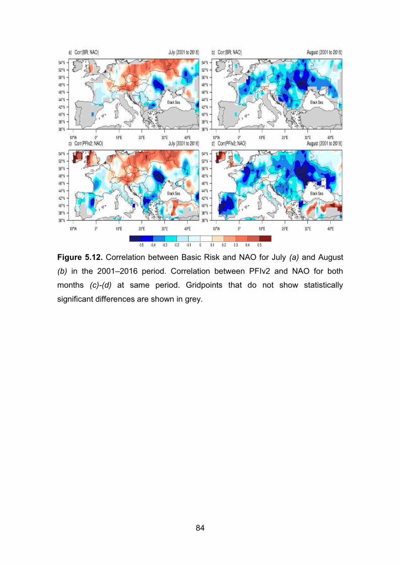
84
Figure 5.12. Correlation between Basic Risk and NAO for July (a) and August
(b) in the 2001–2016 period. Correlation between PFIv2 and NAO for both
months (c)-(d) at same period. Gridpoints that do not show statistically
significant differences are shown in grey.

85
Figure 5.13. Correlation of individual and combined PFIv2 factors with NAO for
SC01 (a)-(d) and SC02 (e)-(h). Gridpoints that do not show statistically
significant differences are shown in grey.

86
CAPÍTULO 6
ARTIGO PROPOSTO
TROPICAL WILDFIRE RISK PERFORMED BY THE POTENTIAL FIRE INDEX
VERSION 2
A. Silva
Agricultural Engineering Department, Federal University of Vicosa, Brazil.
F. Justino
Agricultural Engineering Department, Federal University of Vicosa, Brazil.
A. Setzer
Fire Program of the National Institute of Space Research (INPE), Brazil.

87
ABSTRACT
Fire activities over tropical regions have been induced several impacts on
civilizations and ecosystems. These events are probably the main contributors
in the ensuing agricultural and economic disturbances. Based on atmospheric
susceptibility to fire, this study discusses the climatological El Nino Southern
Oscillation (ENSO) aspects associated with the Potential Weather Fire Index
version 2 (PFIv2). The response of fires to the ENSO is complex and has not
been evaluated systematically across different continents. Here we use ERA-
Interim Reanalysis and CPC Unified Precipitation as input data for the 1998-
2018 period. It has to be noticed that the PFIv2 estimates the risk by
considering local factors such as latitude, and topography profile. We
demonstrate that PFIv2 has revealed an efficiency by up to 70% in presenting
observed fires from Terra/MODIS satellite, over tropical regions, mainly in South
America, and Africa. To evaluate in further details the PFIv2 performance, two
extreme ENSO occurrences are considered. The first event is a La Nina
occurred in 2011 (CS01), and the second is an El Nino in 2015 (CS02). In the
CS01 event, the PFIv2 increases by up to 10%, over the highest fire
concentration in South America, between 40°S and 15°N, related to the direct
influence of atmospheric instability, lower relative humidity, and precipitation
deficit. During the CS02 event, there is an increase (decrease) variation of air
temperature, over northern Australia (southern Africa), and dry conditions are
dominant over most part of South America. The PFIv2 reveals accuracy in
reproducing the regions with fire activity in northern South America, and
southeastern Africa. Further analyzes indicate that there is no correlation
between the ENSO and the PFIv2 with the highest fire occurrences when all
period is considered. On the other, in the CS01 (CS02) negative (positive)
correlations between the ENSO and the PFIv2 (statistically significant at 95%)
were found. This study indicates that the PFIv2 is able to be applied on a variety
of meteorological and time scales.
Keywords: Fire, El Nino, La Nina, tropical, atmospheric conditions, basic risk.
88
1. Introduction
Wildland fire is vital in shaping the earth system properties and have
widespread impacts on climate cycle and human health (BOWMAN et al., 2009;
JOHNSTON et al., 2012; HOLLMANN et al., 2013). Fires affect global climate
through changes in greenhouse gases, vegetation and soil carbon stocks
(BODEN et al., 2017).
The occurrence of fire in vegetation can be described as any fire activity
on the landscape that consumes natural resources, regardless of the source of
ignition (YORK et al., 2012). It has the ability to cause significant damage to an
ecosystem or it can help keep it, make it more resilient. However, managed
forest fire is largely determined by the conditions under which fire exists and the
expected or desired results of management efforts. Fire hazard classification
systems allow land managers to assess the environmental conditions that
contribute to the fire (or potential) hazard and fire distribution (STOCKS et al.,
1996; JUSTINO et al., 2013).
Sectors of society have expressed concern over the indiscriminate use of
wildfire because vegetation wildfires are prominent in issues involving past and
future climate change (e.g. HARRISON et al., 2007). The amount of biomass
burned annually from all sources is about 9.2 billion tons of which 5.13 billion
tons are consumed by global fires in vegetation (FAO 2006). Over 80% of the
global area burned occurs in grasslands and savannas, primarily in Africa and
Australia but also in South America (CHEN et al., 2017).
According to Costa et al (2007), the burning of biomass in ecosystems
due to the expansion of the agricultural frontier, the conversion of vegetation in
pastures, and the renewal of agricultural crops, are some of the most important
factors that cause impacts on climate and biodiversity. The fires still cause the
impoverishment of the soil, the destruction of the vegetation, erosion problems
and they are linked to alterations in the chemical composition of the atmosphere
(YORK et al., 2012).
In fact, the distribution and ecological properties of many biomes in the
world are significantly affected by fire regimes (BOND et al., 2005). Weisse and
Goldman (2018) showed that the annual losses of green forests reached levels
of 29.7 million hectares in 2016, however deforestation showed trends of

89
reduction for the period between August 2016 and July 2017, due to
environmental preservation and ecological planning areas.
The main cause of natural fire proceeds from lightning activities. Globally,
however, human activity is the most burnt cause (WHITLOCK, 2004).
Nevertheless, there is a lively debate on the importance of anthropogenic and
climate forcing in contributing to the ignition of wildfires (HUANG et al., 2015).
Recent advances in atmospheric-ocean coupled circulation modeling
have led to the development of numerical models (global climatic models,
GCMs) that produce dynamic forecasts on the seasonal scale (DOBLAS-
REYES et al., 2013). The potential of such forecasting systems to inform
decision-makers in different economic sectors is enormous due to the provision
of a large number of physically consistent variables, on a broad temporal scale
(MANZANAS et al., 2014). Although large improvements have been achieved in
the estimation of fire risk (MOUILLOT et al., 2005; GIGLIO et al., 2016), it is still
challenging to accurately estimate it using the conventional models. In recent
decades, several computer-based studies have been arguing for fire role as a
dynamical factor influencing large-scale variations in woody vegetation cover in
the tropics (MURPHY and BOWMAN, 2012; DANTAS et al., 2015).
Under current condition, Kloster et al (2010) found the best agreement
between simulation and observations for the fire by explicitly considering human
caused ignition and fire suppression as a function of population density.
Pechony and Shindell (2010) have also found it, however, they added
temperature, precipitation, relative humidity, lightning activity and land cover
datasets. They argued that future climate conditions will play the major role in
driving global fire trends, overcoming the human effect on fire ignition. It has
also been demonstrated that increased surface soil moisture conditions limit the
extent of burned area (LEHSTEN et al., 2010).
Whitlock et al. (2006) have attributed the variations of the fire regime in
the Andes to interannual increase in climate variability and the intensification of
the El Nino South Oscillation (ENSO). According to CHEN et al (2017), ENSO is
a periodic variation in the coupled ocean-atmospheric system with unusually
warm (El Nino) and cold (La Nina) sea surface temperature (SST) in the tropical
eastern Pacific, affecting the atmospheric conditions over the continents. In
most of the tropics, fires are usually limited to the dry season or periods of

90
unusual drought associated with ENSO events (HOFFMANN et al., 2009). The
response of fires to the ENSO is complex and has not been evaluated
systematically across different continents. Here, we consider a threshold of +/-
0.5 °C for the Oceanic Nino Index (ONI), which uses a 3 month running mean of
SST anomalies in the Nino 3.4 region (5°S – 5°N; 120° - 170° W)
(TRENBERTH et al., 2019).
With the lack of available observational data of sufficient length, models
which account for interactions among multiple fire drivers may be used to
provide information about how fires respond tropically to variations in climate
across timescales. Dynamic models have been used to simulate the
interactions between climate variability and fire occurrences (WARD et al.,
2016). However, the large number of degree of freedom arises criticism towards
the need to include several parameters for simulating it (BRADSTOCK, 2010;
SOPKO et al., 2016).
This study aims to investigate how changes in climate by ENSO events
impact the fire risk in the tropical region (atmospheric susceptibility to fire
initiation) during the 1998-2018 period. The method proposed here is built on
the Potential Weather Fire Risk version 2 (PFIv2), presented by Silva et al
(2019). This is a simplified index based on four factors to calculate the risk of
fire. It uses a logistic growth function, which inserts three atmospheric layers,
the local altitude as addressed on Haines Index (1988), and a correction factor
of the air temperature due to latitudinal change. The incidence of seasonal fires
on high and critical classes of the PFIv2 highlight the efficiency to show the
atmospheric conditions linked to fire occurrences. The student’s T-test is
applied to the anomalies in precipitation, and linear correlations among ENSO
and all PFIv2 factors are also performed on study of cases. It must be noted
that the ignition of fires is not taken into account, so that the risk is only potential
in this respect.
The paper is organized as follows: descriptions of the vegetation, climate
data, modelling formulation, and the validation methods in section 2. Section 3
is dedicated to results and discussion. Section 4 provides the capability of the
PFIv2 in reproducing two cases of erratic fires in La Nina (2011) and El Nino
(2015), respectively. The conclusions are described in Section 5.

91
2. Experimental design and model description
The PFIv2, proposed by Silva et al (2019) is applied on tropical region
(Figure 6.1a), over three subdivisions: (I) South America (40°S:15°N;
90°W:30°W); (II) Africa (40°S:15°N; 20W:60°E); and (III) Australia (40°S:15°N;
65°E:180°E). Information on the types of vegetation required for the
computation of PFIv2 were obtained from the classification of the International
Geosphere-Biosphere Programme (IGBP), as shown in Figure 6.1b.
The calculation of the Potential Weather Fire Index version 2 (PFIv2) is
conducted based on the ERA-Interim Reanalysis (DEE at al., 2011), and on the
CPC Unified Precipitation Project (Xie et al., 2010) that is underway at National
Oceanographic and Atmospheric Administration Climate Prediction Center
(NOAA / CPC) for the 1998-2018 period. The spatial resolution of the ERA-
Interim Reanalysis (ERAI) is 1° latitude and longitude grid in the regions of the
tropics.
The CPC spatial resolution is 0.5° latitude and longitude grid over tropical
land areas. This gauge-based analysis of daily precipitation uses reports from
over thousands of stations that are collected from multiple agencies. Historical
records, independent information from measurements at nearby stations, radar
and satellite observations, as well as numerical model forecasts are applied in
the quality control of the data.
It has been used the daily Optimum Interpolation Sea Surface
temperature (OISST) in the Nino3.4 region (5°S:5°N; 120°:170°W) from the
NOAA (TRENBERTH et al., 2019) to build a climatology of El Nino and La Nina
years over a 21-year period from 1998 to 2018. The Nino3.4 SST anomaly
index was calculated using Oceanic Nino Index (ONI). It is based on a threshold
of +/- 0.5°C on 3 month running mean anomalies in the Nino3.4 region.
2.1. Potential Weather Fire Index version 2 (PFIv2)
The Potential Weather Fire Index version 2 (PFIv2) proposed by Silva et
al (2019) includes a modified Haines Index (HAINES, 1988) embedded to a
logistic growth function, and a temperature correction factor due to latitudinal

92
variation to capture the wildfire risk estimates consistent with those observed in
tropical regions. Its final formulation combines three parameters (Equation 6.1).
PFIv2 = BR x (a2 x LF + b) x (RT x Forb) (eq. 6.1)
Where b = 1.3 and the variables Basic Risk (BR) and Run Temperature
(RT) are the same as in the original index (JUSTINO et al., 2010; 2013), but the
constant a2 = 0.006. The term (a2 x LF + b) is the impact factor of the Haines
logistic function (Loghai), and the variable Forb = (0,003 x |Lat| + 1) is a
correction factor of the air temperature for latitudinal change. The sequence of
PFIv2 calculations is shown in Figure 6.2. It is important to mention that the
PFIv2 categories range from 0 to 1 (Table 6.1).
Active wildfire products from NASA’s MODIS (2001 to 2018) will be used
to verify the capability of the PFIv2 for detecting the most susceptible region for
erratic wildfires development. The wildfire products from the sixth collection of
moderate-resolution spectral images of the Terra/MODIS includes algorithms
for the elimination of false alarms, like those caused by the deforestation of
small forests, precision in the detection of wildfires of reduced spatial scale,
adjustment for the presence of cloudness and rejection expanded brightness of
the sun. The products from Terra/MODIS are defined in a sine grid of the Earth
to the spatial scales of 250-m, 500-m, or 1-km.
Fires detected by Terra/MODIS satellite were computed and reclassified
seasonally during the 2001-2018 period. The time scale was selected according
to the negative and positive phases of the El Nino Southern Oscillation (ENSO),
as proposed by Trenberth et al (2019). Figure 6.3 shows the specific years with
sea surface temperature higher than 0.5°C (El Nino) and that ones lower than -
0.5°C (La Nina).
The validation of the PFIv2 versus satellite-derived wildfire can be carried
out by checking the number of wildfires located in the high and critical wildfire
risk grid. Evaluation of the wildfire risk based on PFIv2 may be validated with
other satellite as well. For instance, GOES and NOAA products can be utilized.
The limitation in satellite wildfires detection is that most of these products are
not available prior 2000.

93
3. Results and Discussion
3.1. Sea surface temperature and precipitation variabilities
Figure 6.4(a) shows the climatology of the sea surface temperature
(SST) in the 1998-2018 period. The Nino 3.4 region which is highlighted over
tropical eastern Pacific, is linked to atmospheric conditions over the continents.
According to McPhaden et al (2006), this climate variability has a pronounced
influence on year-to-year variations in climate. The selected data presenting
positive and negative phases of the ENSO from ONI methodology show well-
defined La Nina (Figure 6.4b) and El Nino (Figure 6.4c) events. Although the
differences in SSTs between El Nino and La Nina were largest during June-
April, strong positive and negative anomalies were found beyond the end of the
El Nino and La Nina SST anomalies.
Recently, Chen et al (2017) showed that ENSO leads changes in the
precipitation regimes over the tropical region. In fact, the timing and magnitude
of the modified pattern of precipitation alters the landscape fire activity, with
larger interannual variability in fires. According to Justino et al (2010),
precipitation plays a key role on the Potential Weather Fire Index. For inserting
a drought factor which is calculated by daily rainfall. The interannual variability
of fires responds to the positive (negative) El Nino-South Oscillation (ENSO)
phase such as in 2001, 2009 and 2014 (in 2005, 2007, 2008 and 2010). ENSO
events cause changes on the regional Hadley and Walker cells that influence
negative anomalies of precipitation in northeastern South America.
Figures 6.5 show the anomalies in precipitation for El Nino and La Nina
events, based on CPC data in the 1998-2018 period. During the El Nino events,
reductions around 1.5 mm/day are verified in the precipitation over central and
northern regions of the South America, in subtropical Africa, and Australia
(Figure 6.5a). Thus, the ENSO positive phase contributes to the intensification
of the BR in these areas due the short amount of precipitation with respect to
present climatology. Although, opposite signals closest to 1.5 mm/day at 95%
significance levels are shown in southern Brazil, Patagonia, and Madagascar.
These findings are similar from the results found by Curtis and Adler (2003). On
the other hand, the overestimation of precipitation differences during La Nina

94
events has potential to weak the conditions of fire activity over the tropical
region, in particular in northern Brazil and Australia (Figure 6.5b). These
differences present opposing responses to ENSO, and this limited the degree of
predictability at a continental scale.
3.2. Climatology in the 1998-2018 period
Figures 6.6(a)-(c) show the 1998-2018 climatologies of air temperature,
relative humidity, and surface pressure from ERA-Interim reanalysis for the
tropical region. Similarly, the individual climatologies of the precipitation, and
basic risk of fire (BR) from CPC are presented in Figures 6.6(d)-(e). The factors
of the PFIv2, and the final modelling are shown in Figures 6.6(g)-(h).
In the tropical troposphere, the temperature gradients are weaker than in
extratropical regions, so the term of horizontal advection is minimal and the
temperatures in some specific localities vary slightly from one day to the next
(Figure 6.6a). On the other hand, Figures 6.6 (b)-(c) show that the rates of
diabatic warming in the tropical convection regions are higher than those
typically observed in the medium and high latittudes. In Figure 6.6(d) is
observed that the values closest to 8 mm/day are consistent with the upward
movement concentrated in precipitation belts, such as the Intertropical
Convergence Zone (ITCZ), where heating due to latent heat released by
condensation is practically compensated by the cooling induced by vertical
velocity.
In the tropical region, in addition to the southern circulation resulting from
the activity of Hadley cells, there is a large-scale zonal circulation due to
Walker's cells (PHILANDER, 1990). This circulation is attributed basically to the
differential warming that occurs between the continents and oceans, having
been better understood in the southern hemisphere, due to the greater
distribution of continental areas in the northern hemisphere.
In the individual climatologies of the PFIv2 factors, it is noted that the BR
(Figure 6.6e) governs fire risk. It is worth mention that this factor considers the
precipitation frequency of occurrence in the last 120 days before the due date in
association with the type of vegetation. This is consistent with some recent
studies which have addressed the arising on fires to the anthropogenic

95
vegetation changes (SILVA et al., 2003; DAVIDSON et al., 2012; SPERA et al.,
2016).
Figure 6.6(f) displays that the Haines logistic factor contributes more
effectively in Chile, southern Africa, central and western Australia. Figure 6.6(g)
shows that the influence of temperature is most dominant over the South
America, mainly in Brazil. This cleary reveals that regions such as northern
South America, subtropical Africa and northern Australia have an atmosphere
conducive to burning seasonally which can be enhanced due to anomalous
conditions, such as heat waves and droughts.
Figure 6.6(h) shows the climatological distribution of the PFIv2. It is clear
that the BR dominates the continental distribution. Most part of South America
and southern Africa are very vulnerable for fire development related to dry
conditions in particular between July and September. In the following the
changes on this parameters by ENSO events are investigated in details, to
verify the PFIv2 capability to reproduce extreme events in fire activity.
3.3. The El Nino Southern Oscillation (ENSO) and the fire activity
Over tropical latitudes, the climate regime is mainly dictated by vacillation
in the phase of the ENSO. This natural phenomenon shows interannual sea
surface temperature and air pressure anomalies in the Tropical Pacific (DESER
et al., 2010). When it comes to SST variability related to ENSO, variations
induce to precipitation changes in the Tropical Pacific Ocean. This local
variability is crucial on global climate changes (ZHOU et al., 2014). Extreme
changes in SST over the tropical Pacific characterize the influence of the inter-
tropical Atlantic SST gradients as being significant in modulating the influence
of ENSO by intensifying the Southern Atlantic Convergence Zone (SACZ) and
Intertropical Convergence Zone (ITCZ).
The oceanic and atmospheric conditions in the Tropical Pacific Ocean
have been changed irregularity between warm (El Nino) and cold (La Nina)
phases. During El Nino periods, the air surface pressure get high up to typical
patterns from Australia, South America, and Africa, inducing dry periods. These
conditions also act in northeastern Brazil and southern Africa. On the other
hand, low pressure are developed in the central and east regions of Pacific,

96
across western South America coast. In winter, heavy precipitation and flooding
are commonly observed near Uruguay. Similarly, dry regions during El Nino
tend to be characterized by elevated humidity on La Nina occurrences.
Figure 6.7(a) shows the average Basic Risk (BR) for El Nino events in
the 1998-2018 time period. Due to the importance of precipitation to the fire risk,
the BR contributes of up to 0.85 to the final fire risk. As expected, analyses for
the Haines factor (Figure 6.7b) tend to highlight the regions dominated by dry
conditions and susceptible to convection. This is shown by larger differences of
the stability and humidity parameters according to the altitude of the grid point.
When it comes to temperature factor (Figure 6.7c), it is demonstrated
that the most susceptible regions for fire occurrence are located in South
America. This might be expected because the Atlantic Subtropical High extends
toward the continent, which causes the subsidence of the air and dry wheater
conditions (FETTER et al., 2018). It is important to mention that the PFIv2
reasonable reproduces the role of the climatic conditions implicit in the method.
For example, the central region of Brazil is dominated by a high contribution of
the temperature factor (Figure 6.7c), but low to medium BR values. Thus, the
PFIv2 delivers to minimum values. Under northeastern Brazil these factors are
proportional and the response is direct (Figure 6.7d).
The south part of Africa revealed that the four PFIv2 parameters are in
favor for fire occurrence, due to low precipitation, dry atmospheric conditions
and susceptible vegetation pattern. Figure 6.7(d) also shows that there are
favorable conditions for the fire risk due to BR in Australia, however, the
contributions of the Haines logistic factor (Figure 6.7b) and the temperature
factor corrected by the latitudinal effect reduce the PFIv2 to levels (Figure 6.7d).
Figure 6.7(e) shows the standard deviation (STD) of the tropical PFIv2. It
is observed that a latitudinal gradient is constructed in sub-Saharan Africa and
northern South America. In addition, higher variability is also observed in the
central part of Brazil, and subtropical Africa.
In the same way, Figures 6.7(f)-(j) show the differences between the El
Nino and La Nina events. This highlights that under El Nino conditions there are
higher contribution to the intensification of fire risk than in La Nina. Furthermore,
it is clear that the BR (Figure 6.7f) has the main contribution to elevate the final

97
index. It can be noted that the Haines and temperature factors play specifically
over the most susceptible areas (Figures 6.7g-h).
Turning to the PFIv2 anomaly (Figure 6.7i), it is emphasized that the
reduction in precipitation during the El Nino characterizes the highest prominent
regions, mainly in northern South America, southern Africa and Australia. In
consequence, these areas also have the most risk fire variations, as showed by
the STD (Figure 6.7j).
In order to validate the PFIv2 results, Figure 6.8 shows the capability of
the PFIv2 model in locating the daily fires of the Terra/MODIS satellite, based
on both ENSO phases. This verification is done by comparing if the fire position
is coincident with the highest PFIv2 levels (between 0.7 and 1). The ideal
metrics would be that in which the PFIv2 shows all fire occurrences at the
critical level (grater than 0.95). Figure 6.8(a) shows that the PFIv2 reasonable
finds the annual variability that may be understood by the predominance fires in
the highest classes (high and critical). The total number of fires detected on
these classes are 66.5% and 58.4% in La Nina and El Nino, respectively. This
soft unexpected difference is explained by the higher frequencies of La Nina in
the period, and also by the precipitation dataset that has been constantly
improved for tropical latitudes and by the anthropic effect in advancing
agricultural boundaries.
It is important to mention that Africa which is the continent with the
highest fire occurrences presents the highest levels in fire detection (Figure
6.8b). Among the regions analysed, Australia (Figure 6.8c) was the subregion
that presented the lowest variability among the risk classes. This is because the
seasonal range of fire occurrences is high in Australia, whose observations
differ approximately 100 thousand observations between the March and
October interval.
To identify the main teleconnection patterns between the ENSO and
PFIv2, the Pearson correlation (WILKS, 2006) is used (Figures 6.9). It is a
dimensionless index with values raging from -1.0 (inverse proportional) to 1.0
(directly proportional) which reflects the intensity of a linear relation between
two dataset. As previously mentioned, differences on timing and magnitude
scales of the events highlighted the regions favorable to burn, but also brings
challenges to future scientific studies. Figure 6.9(a) displays the strong positive

98
influence of the ENSO on the PFIv2 over northern South America, southern
Africa, and northern Australia. Under La Nina conditions (Figure 6.9b), the
mainly contribution occurs in central part of Brazil, which usually experiences
high levels of fire between July and September interval. Similarity, the high
susceptibility of fire is located over subtropical Africa. In summary, the
correlation are presenting reasonable the dipoles between both events, this can
be noted over southern Africa, northern and southern Brazil.
Thus, the following section discusses the application of the PFIv2
methodology in the analysis of extreme events of fire occurrences in La Nina
and El Nino events. This applicability aims at reducing the challenges
encountered by decision makers, in fire activity forecasting.
4. Case Studies
After verifying the PFIv2 capability to locate the main regions of fire
activity, it is applied to extreme fire occurrences in La Nina and El Nino
occurrences. The first event analyzed is the erratic fires in tropical region during
La Nina 2011 (CS01). The second event (CS02) is under an El Nino event in
2015 (CHEN et al., 2017).
Figures 6.10 show the distribution of the SST on the following analyses:
climatology for the 1998 to 2018 period (Figure 6.10a); anomalies in the La Nina
(Figure 6.10b); and in the El Nino (Figure 6.10c). The cold (warm) conditions of
the central Pacific in CS01 (CS02) exhibits a remarkable magnitude to change
all individual and combined PFIv2 factors.
4.1. Tropical fire risk and the La Nina 2011 (CS01)
Figures 6.11(a)-(d) depict the climate anomalies during the CS01 event,
in relation to the 1998-2018 climatology. The CS01 exhibits a remarkable
cooling over northeastern Brazil, southeastern Africa, and northern Australia
(Figure 6.11a). These atmospheric conditions are proportional to the relative
humidity and precipitation (Figures 6.11b,d), except for the central and
northwestern parts of Brazil where temperature differences were about 1.5°C
higher, compared to climatological values.

99
As should be expected from the relationship between temperature and
relative humidity, warmer conditions result in a drop of relative humidity by up to
8% over southern Africa and Australia (Figure 6.11b). In addition, the surface
pressure decreases (Figure 6.11c), which even favors wet conditions
consequently intensifying precipitation (Figure 6.11d). Reduction of precipitation
is more proeminent in southern South America, central part of Africa, values
much close to the climatology appear in the southeastern Brazil (Figure 6.11d).
It is worth noting that the first component to be considered in the PFIv2
is the BR, which depends on daily accumulated precipitation data. However,
there are not proportional rates (in magnitude) of the anomalous precipitation
regime (Figure 6.11d) and the BR distribution. The BR considers a period of up
to 120 days before the beginning of the analysis. Therefore, it is evident that the
increase in precipitation over northeastern South America, southeast region of
Africa, and Australia were specific occurrences from CS01. On the other hand,
there is a predominance level closest to 0.6 in BR near the southern region of
Patagonia (Figure 6.11e).
In relation to the Haines logistic factor (Figure 6.11f), it is observed a
similar distribution to that demonstrated by the relative humidity (Figure 6.11b),
in which most of tropical region is neutral or favorable to fire development,
except in Australia. Figure 6.11(g) presents the contribution of the temperature
factor to the risk of fire in the CS01 interval. Similarly to temperature anomalies
(Figure 6.11a), this parameter suggests that from the central part of Brazil to
northwestern South America fire was susceptible to occur. However, the PFIv2
anomaly between the CS01 and the 1998-2018 period, over eastern Brazil,
southern Africa, and northern South America show condition of lower
vulnerability, but as will be discussed below, fire incident was remarkable over
there.
As shown in Figure 6.11(h), the PFIv2 decreases by up to 0.15, in
Australia, and southern Africa between 40°S and 20°S. However, the southern
South America experiences massive number of fires, related to direct influence
of local elevation and atmospheric conditions such as much, lower relative
humidity, and precipitation.

100
4.2. Tropical fire risk and the El Nino 2015 (CS02)
Figures 6.12(a)-(h) show the difference of climate and PFIv2 components
with respect to the 1998-2018 interval characteristics of the CS02 event. At the
case of meteorological anomalies, Figure 6.12(a) presents a positive variation
of air temperature at 2m, along the 40°S and 15°N latitudinal belt. Warmer
conditions of up to 1.5°C are evident in South America, subtropical Africa, and
western Australia.
As expected, the spatial pattern of relative humidity (Figure 6.12b) is
correlated to that of the air temperature at 2m. It is worth to mention that
positive (negative) anomalies of relative humidity (air temperature at 2m) act in
most of tropical region to enhance the fire vulnerability. The lowest pressure
anomalous patterns are over Patagonia and southeastern part of South
America (Figure 6.12c) increases the atmospheric humidity.
Turning to precipitation (Figure 6.12d), there is a clear relationship
among low pressure regions as previously observed in South America (Figures
6.12c,d). Conversely, dry conditions are dominant over most part of Brazil and
Australia. Figure 6.12(e) shows the BR anomaly during the CS02, in relation to
the 1998-2018 period. It is interesting to note that positive anomalies of BR are
located in regions of different meteorological patterns, such as in southern
Brazil. It is also observed that the northeastern Brazil shows positive anomalies
close to 0.3, which reflects the drop in precipitation in Figure 6.12(d). The
absence of proportional links between the precipitation (Figure 6.12d) and the
BR (Figure 6.12e) over the central region of Africa may be explained by the fact
that the anomalies are specific to the El Nino event. The distribution of the
precipitation is an important parameter in the PFIv2, for the BR calculation takes
into account the precipitation data that are accumulated in distinct intervals in
the 120 days prior to the first day of the analysis.
As shown in Figures 6.12(f)-(g), the respective Haines logistic and
temperature factors can efficiently reproduce regions which are prone to fire
development. Both functions tend to concentrate the higher atmospheric
vulnerability to burn. Figure 6.12(f) highlights prominent regions of Brazil and
the southern Africa. In addition, Figure 6.12(g) shows that the temperature

101
factor also plays an important role in detecting the contribution by the latitudinal
changes.
The anomaly of the PFIv2 reveals accuracy in the range of accumulated
fires in northern South America, southwest Africa and some localities in
northern Australia during the CS02 (Figure 6.12h), in agreement with the fire
occurrence. The negative anomaly observed from the southern to western
South America coast, and in central part of Africa arise due to the anomalous
characteristics of precipitation and humidity in the CS02. Hundreds of
accumulated fires in these areas does not match positive PFIv2 anomalies.
4.3. Accumulated daily fire in the CS01 and CS02
Finally, to validate the PFIv2 results in the CS01 and CS02, Figures 6.13
show the capability of the PFIv2 model in locating the daily fires of the
Terra/MODIS satellite, based on both ENSO phases. Due the quality on satellite
information, this verification is restricted for the 2001-2018 period, by comparing
if the fire position is coincident with the highest PFIv2 levels (between 0.7 and
1).
Figure 6.13(a) confirms that our previously climate analyses were
consistent, showing a higher fire detection in South America during an El Nino
event. The difference between the efficiency of El Nino and La Nina reached
values around 15%. In Africa, the efficiency of the PFIv2 was reasonable
demonstrated with 71.6% and 72.3% of the total accumulated daily data over
the critical class in the CS01 and CS02, respectively.
As discussed on Figures 6.8, among all regions analyzed, Australia has
the highest sazonal variability in fire occurrences. It is important to mention that
values near to 11% detected in the minimum class may be associated with
previous environmental conditions. Despite this characteristic, the PFIv2
detected up to 64.8% of the fire occurrences only in the critical class in the
CS02 (El Nino) event.

102
5. Conclusions
Based on the Potential Weather Fire Index version 2 (PFIv2), this study
evaluated the tropical susceptibility to the fire occurrences, according to current
atmospheric patterns. It was demonstrated that the PFIv2 could reasonable
reproduce the annual variability of the fire occurrences in South America, Africa,
and Australia. Two case studies were investigated in order to validate the
PFIv2: (i) In the La Nina occurred in 2011 and; (ii) in the El Nino from 2015.
The findings elucidate that the modifications proposed on the PFIv2 to
improve the prediction of fire risk over the extratropical regions also contributed
to the current quality of the original version in detecting regions favorable to fire
occurrences in tropical regions. This was verified, mainly in the Africa continent,
with accuracy level in the maximum classes up to 73% and 75% under La Nina
and El Nino events, respectively.
The most important limitation of PFIv2 is the high dependence of the
days of dryness, which is computed from the precipitation data. For precipitation
is still an uncertain parameter in the forecasts of the present climate and also
presents divergences among the atmospheric models. However, it was
demonstrated that the CPC dataset is reasonable to detect the climate
variabilities.
It is known that the majority of present day fires have an anthropogenic
origin. However, the results presented in this paper are entirely independent of
human action and are based only upon the atmospheric vulnerability to the
occurrence of fire. Nonetheless, increased fire weather in a changing climate
will be one of many ingredients that will continue to shape changes in fire
activity. Despite different manners to start and maintain fire, climatic conditions
need to be favorable to the fire occurrences.
6. Acknowledgements
To the people management of the Federal University of West Para
(Ordinance N ° 594, of March 4th, 2015). To the Graduate Program in Applied
Meteorology of the Federal University of Vicosa (www.posmet.ufv.br) and to the

103
Fire Program of the National Institute of Space Research (INPE) – Brazil
(http://www.inpe.br/queimadas/portal).
REFERENCES
BOND, W. J., WOODWARD, F. I., and MIDGLEY, G. F. The global
distribution of ecosystems in a world without fire. New Phytologist, v. 165, p. 525-537, doi: 10.1111/j.1469-8137.2004.01252.x, 2005.
BODEN, T. A., MARLAND, G., and ANDRES, R. J. Global, Regional, and
National Fossil-Fuel CO2 Emissions. Carbon Dioxide Information Analysis Center, Oak Ridge National Laboratory, U.S. Department of Energy, Oak Ridge, Tenn., U.S.A., https://doi.org/10.3334/CDIAC/00001_V2017, 2017.
BOWMAN, D. M. J. S. et al. Fire in the Earth system. Science, v. 324, p.
481-484, 2009. BRADSTOCK, R. A. A biogeographic model of fire regimes in Australia:
current and future implications. Global Ecology and Biogeography, 19, 145-158. doi: 10.1111/j.1466-8238.2009.00512.x, 2010.
CHEN, Y. et al. A pan-tropical cascade of fire driven by El Niño/Southern
Oscillation. Nature Climate Change, v. 7, p. 906-911, doi:10.1038/s41558-017-0014-8, 2017.
COSTA, M. H., YANAGI, SILVIA, N. M., SOUZA, P. J. O. P., RIBEIRO,
A., ROCHA, E. J. P. Climate change in Amazonia caused by soybean cropland expansion, as compared to caused by pastureland expansion. Geophysical Research Letters, Vol. 34, p. L07706, 2007.
CURTIS, S., and ADLER, R. F. Evolution of El Niño-precipitation
relationships from satellites and gauges. J. Geophys. Res., 108, 4153, 2003. DANTAS, V. L., HIROTA, M., OLIVEIRA, R. S., and PAUSAS, J. G.
Disturbance maintains alternative biome states. Ecology Letters, v. 19, p. 12-19, 2015.
DAVIDSON, E. A., de ARAÚJO, A. C., ARTAXO, P., BALC, J. K.,
BROWN, l. F. et al. The amazona basin in transition. Nature, v. 481, n. 7381, p. 321-328, 2012.
DEE, D. P., UPPALA, S. M., SIMMONS, A. J., BERRISFORD, P., POLI,
P. et al. The ERA-Interim reanalysis: Configuration and performance of the data assimilation system. Quarterly Journal of the Royal Meteorological Society, v. 137(656), p. 553-597, 2011.
DESER, C., XIE, S-P., ALEXANDER, M. A., and PHILLIPS, A. S. Sea
surface temperature variability: patterns and mechanisms. Annual Review of
104
Marine Science, v. 2, p. 115-143, doi: 10.1146/annurev-marine-120408-151453, 2010.
DOBLAS-REYES, F. J., GARCÍA-SERRANO, J., LIENERT, F.,
BIESCAS, A. P., and RODRIGUES, L. R. L. Seasonal climate predictability and forecasting: status and prospects. Wiley Interdisciplinary Rev.: Climate Change, Vol. 4, p. 245-268, 2013.
FAO. Fire management global assessment. A thematic study prepared in
the framework of the Global Forest Resources Assesment. Food and Agriculture Organization of the United Nations, 2006.
FETTER, R., CARLOS, H., and STEINKE E. Um Índice para Avaliação
da Variabilidade Espaço-Temporal das Chuvas no Brasil. Revista Brasileira de Meteorologia, n. 2, p. 225-237, 2018.
GIGLIO, L., SCHROEDER, W., and JUSTICE, C. O. The collection 6
MODIS active fire detection algorithm and fire products. Remote Sensing of Environment, v. 178, p. 31-41, 2016.
HARRISON, S. P., POWER, M., and BOND, W. Paleofires and the Earth
system. iLEAPS Newsletter, v. 3, p. 18-20, 2007. HOFFMANN, A. A., PARRY, J., CUAMBE, C., KWESHA, D., and
ZHAKATA, W. Climate change and wildland fires in Mozambique. In M. A. Cochrane (Ed.), Tropical Fire Ecology: Climate Change, Land Use, and Ecosystem Dynamics. Springer/Praxis, Heidelberg, Germany/Chichester, U.K., 2009.
HOLLMANN, R., MERCHANT, C., SAUNDERS, R., DOWNY, C. et al.
The ESA climate change initiative: satellite data records for essential climate variables. Bulletin of the American Meteorological Society, 94, p. 1541-1552, 2013.
HUANG, X., REIN, G., and CHEIN, H. Computational smoldering
combustion: Predicting the roles of moisture and inert contents in peat wildfires. Proceedings of the Combustion Institute, v. 35, p. 2673-2681, 2015.
JOHNSTON, F. H. et al. Estimated Global Mortality Attributable to Smoke
from Landscape Fires, Environmental Health Perspectives, v. 120, p. 695–701, https://doi.org/10.1289/ehp.1104422, 2012.
JUSTINO, F., STORDAL, F., CLEMENT, A., COPPOLA, E., SETZER, A.,
and BRUMATTI, D. Modelling Weather and Climate Related Fire Risk in Africa. American Journal of Climate Change, 2, p. 209 – 224, 2013.
KLOSTER, K et al. Fire Dynamics During the 20th Century Simulated by
the Community Land Model, Biodigeosciences, Vol. 7, No. 6, p. 1877-1902, 2010.

105
LEHSTEN, P., HARMAND, P., PALUMBO, I., and ARNETH, A. Modelling Burned Area in Africa, Biogeosciences, Vol. 7, p. 3199-3214, 2010.
MANZANAS, R., FRÍAS, M. D., CONFIÑO, A. S., and GUTIÉRREZ, J. M.
Validation of 40 year multimodel seasonal precipitation forecasts: the role of ENSO on the global skill. Journal of Geophysical Research: Atmospheres, v. 119, p. 1708-1719, 2014.
MCPHADEN, M. J., ZEBIAK, S. E., and GLANTZ, M. H. ENSO as an
integrating concept in Earth science. Science, v. 314, p. 1740-1745, 2006. MOUILLOT, F., and FIELD, C. B. Fire history and the global carbon
budget: a 1° x 1° fire history reconstruction for the 20th century. Global Change Biology, 11, 398 – 420. doi: 10.1111/J.1365-2486.2005.00920.X, 2005.
MURPHY, B. P., and BOWMAN, D. M. What controls the distribution of
tropical forest and savanna? Ecology Letters, v. 15, p. 748-758, 2012. PECHONY, O., and SCHINDELL, D. T. Driving Forces of Global
Wildfires over the Past Millennium and the Forthcoming Century, Proceedings of the National Academy of Sciences, 2010.
PHILANDER, S. G. El Niño, La Niña, and the Southern Oscillation.
Academic San Diego, 1990. SOPKO, P., BRADSHAW, l., and JOLLY, M. Spatial products available
for identifying areas of likely wildfire ignitions using lightning location data-Wildland Spera, S. A., Galford, G. L., Coe, M. T., Macedo, M. N., Mustard, J. F. (2016). Land-Use Change Affects Water Recycling in Brazil’s Last Agricultural Frontier. Global Change Biology, doi: 10.1111/gcb.13298, 2016.
SPERA, S. A., GALFORD, G. L., COE, M. T., MACEDO, M. N., and
MUSTARD, J. F. Land-Use Change Affects Water Recycling in Brazil's Last Agricultural Frontier. Global Change Biology, doi:10.1111/gcb.13298, 2016.
STOCKS, B.J., and LAWSON, B.D. El sistema Canadiense de
evaluacion del grado de peligro de incendios forestales: Una vision general. p. 82-94 in J.A. Guillermo, Editor. Proc. Prognosis Y Gestion en Control de Incendios Forestales, Actas del Taller Internacional, November 8-10, 1995, Santiago de Chile. Proyecto FONDEF FI-13, Santiago de Chile, 1996.
TRENBERTH, K., and National Center for Atmospheric Research Staff
(Eds). The Climate Data Guide: Nino SST Indices (Nino 1+2, 3, 3.4, 4; ONI and TNI). Retrieved from https://climatedataguide.ucar.edu/climate-data/nino-sst-indices-nino-12-3-34-4-oni-and-tni. Last modified 11 Jan 2019.
YORK, A., BELL, T. L., and WESTON, C. J. Fire regimes and soil-based
ecological processes: implications for biodiversity. In Bradstock R. A et al (Eds) ‘Flammable Australia, Fire regimes, biodiversity and ecosystems in a changing world’ (CSIRO Publishing: Collingwood, VIC), p. 127-148, 2012.

106
WARD, D. S., SHEVLIAKOVA, E., MALYSHEV, S., LAMARQUE, J-F.,
and WITTEMBERG, A. T. Variability of fire emissions on interannual to multi-decadal timescales in two Earth System models. Environmental Research Letters, v. 11, doi:10.1088/1748-9327/11/12/125008, 2016.
WEISSE, M., and GOLDMAN, L. 2017 Was the Second-Worst Year on
Record for Tropical Tree Cover Loss. Global Forest Watch. Online available at [https://blog.globalforestwatch.org/data-and-research/2017-foi-o-segundo-pior-ano-ja-registrado-de-perda-de-cobertura-florestal-tropical], 2018.
WHITLOCK, C., and BARTLEIN, P. J. Holocene fire activity as a record of
past environmental change, in: Developments in Quaternary Science, edited by: Gillespie, A. R., Porter, S. C., and Atwater, B. F., Elsevier, Amsterdam, 2004.
WHITLOCK, C., MORENO, P. I., and BARTLEIN, P. Climatic controls of
Holocene fire patterns in southern South America, Quaternary Research, v. 68, p. 28–36, 2006.
WILKS, D. S. Statistical Methods in the Atmosphere Sciences, 2006. ZHOU, Z. -Q., XIE, S. -P., ZHENG, X. -T., LIU, Q., and WANG, H. Global
warming-induced changes in El Niño teleconnections over the North Pacific and North America. Journal of Climate, v. 27, p. 9050-9064, doi: https://doi.org/10.1175/JCLI-D-14-00254.1, 2014.
Tables
TABLE 6.1. Fire risk (PFIv2) levels.
Levels PFI (0 to 1)
Minimum < 0.15
Low 0.15 to 0.40
Medium 0.40 to 0.70
High 0.70 to 0.95
Critical 0.95
Figures
Fig. 6.1 (a) Study areas. (b) Vegetation distribution by IGBP (adapted
from FRIEDL et al., 2010).

107
Fig. 6.2 Flowchart presenting the sequence of calculation for the PFIv2.
Fig. 6.3 Annual series of the ONI from 1998 to 2018. Blue and red lines
are the limit values for La Nina and El Nino, respectively. Souce: OSST/NOAA.
Fig. 6.4 Sea Surface Temperature (SST) climatology in the 1998-2018
period (a). (b) SST anomaly on La Nina events and; (c) SST anomaly on El
Nino events.
Fig. 6.5 Anomalies in CPC precipitation for El Nino (a); and La Nina (b)
events in the 1998-2018 period. Black dots show statistically significant
differences at 95%.
Fig. 6.6 Present day (1998-2018) climatology. Maximum temperature at
2 m ((a), °C), relative humidity (b), surface pressure ((c), hPa), precipitation ((d),
mm/day), PFIv2 factors (e)-(g) and, (h) PFIv2.
Fig. 6.7 PFIv2 factors on El Nino events during the 1998-2018 period (a)-
(d). Figure (e) is the standard deviation. The same sequence is shown from (f)-
(j), but for the difference between El Nino and La Nina events.
Fig. 6.8 Percentage of accumulated daily fire at each PFIv2 for El Nino
and La Nina events in (a) South America, (b) Africa, and (c) Australia in the
2001-2018 period. ZERO indices are the percentage of fire events that were
observed in a level closest to zero by PFIv2 (displayed in the top left corner of
each panel).
Fig. 6.9 Correlation between the PFIv2 and ENSO for El Nino (a), and La
Nina (b) events in the 1998-2018 period. Gridpoints that do not show
statistically significant differences are shown in grey.

108
Fig. 6.10 Sea Surface Temperature (SST) climatology in the 1998-2018
period (a). (b) SST anomaly on a La Nina event (2011) and; (c) SST anomaly
on a El Nino event (2015).
Fig. 6.11 Anomalies in (a) maximum temperature at 2 m (°C), (b) relative
humidity (%), (c) surface pressure (hPa), (d) precipitation (mm/day), (e)-(g)
PFIv2 factors, and (h) PFIv2 distribution for 2011 (La Nina event) with respect to
climatology from 1998 to 2018.
Fig. 6.12 Anomalies in (a) maximum temperature at 2 m (°C), (b) relative
humidity (%), (c) surface pressure (hPa), (d) precipitation (mm/day), (e)-(g)
PFIv2 factors, and (h) PFIv2 distribution for 2015 (El Nino event) with respect to
climatology from 1998 to 2018.
Fig. 6.13 Percentage of accumulated daily fire at each PFIv2 level in (a)
South America; (b) Africa; and (c) Australia on La Nina (2011) and El Nino
(2015) events. ZERO indices are the percentage of fire events that were
observed in a level closest to zero by PFIv2 (displayed in the top left corner of
each panel).

109
Figure 6.1. (a) Study areas. (b) Vegetation distribution by IGBP (adapted from
FRIEDL et al., 2010).
Figure 6.2. Flowchart presenting the sequence of calculation for the PFIv2.

110
Figure 6.3. Annual series of the ONI from 1998 to 2018. Blue and red lines are
the limit values for La Nina and El Nino respectively. Source: OISST/NOAA.
Figure 6.4. Sea Surface Temperature (SST) climatology in the 1998-2018
period (a). (b) SST anomaly on La Nina events and; (c) SST anomaly on El
Nino events. The black box shows the Nino3.4 region.

111
Figure 6.5. Anomalies in CPC precipitation for El Nino (a); and La Nina (b)
events in the 1998-2018 period. Black dots show statistically significant
differences at 95%.

112
Figure 6.6. Present day (1998-2018) climatology. Maximum temperature at 2 m
((a), °C), relative humidity (b), surface pressure ((c), hPa), precipitation ((d),
mm/day), PFIv2 factors (e)-(g) and, (h) PFIv2.

113
Figure 6.7. PFIv2 factors on El Nino events during the 1998-2018 period (a)-
(d). Figure (e) is the standard deviation. The same sequence is shown from (f)-
(j), but for the difference between El Nino and La Nina events.

114
Figure 6.8. Percentage of accumulated daily fire at each PFIv2 for El Nino and
La Nina events in (a) South America, (b) Africa, and (c) Australia in the 2001-
2018 period. ZERO indices are the percentage of fire events that were
observed in a level closest to zero by PFIv2 (displayed in the top left corner of
each panel).

115
Figure 6.9. Correlation between the PFIv2 and ENSO for El Nino (a), and La
Nina (b) events in the 1998-2018 period. Gridpoints that do not show
statistically significant differences are shown in grey.
Figure 6.10. Sea Surface Temperature (SST) climatology in the 1998-2018
period (a). (b) SST anomaly on a La Nina event (2011) and; (c) SST anomaly
on an El Nino event (2015).

116
Figure 6.11. Anomalies in (a) maximum temperature at 2 m (°C), (b) relative
humidity (%), (c) surface pressure (hPa), (d) precipitation (mm/day), (e)-(g)
PFIv2 factors, and (h) PFIv2 distribution for 2011 (La Nina event) with respect to
climatology from 1998 to 2018.

117
Figure 6.12. Anomalies in (a) maximum temperature at 2 m (°C), (b) relative
humidity (%), (c) surface pressure (hPa), (d) precipitation (mm/day), (e)-(g)
PFIv2 factors, and (h) PFIv2 distribution for 2015 (El Nino event) with respect to
climatology from 1998 to 2018.

118
Figure 6.13. Percentage of accumulated daily fire at each PFIv2 level in (a)
South America; (b) Africa; and (c) Australia on La Nina (2011) and El Nino
(2015) events. ZERO indices are the percentage of fire events that were
observed in a level closest to zero by PFIv2 (displayed in the top left corner of
each panel).

119
CAPÍTULO 7
CONCLUSÕES E PERSPECTIVAS FUTURAS
Baseado no Índice de Risco Potencial de Fogo versão 2 (PFIv2), este
trabalho avaliou a suscetibilidade da vegetação ao fogo, segundo as condições
atmosféricas do presente. O índice revelou-se como uma ferramenta útil no
entendimento da distribuição global do fogo em vegetação. Isso só foi possível
devido à base já consolidada do PFI.
Demonstrou-se que a modificação proposta no PFIv2 pôde reproduzir as
regiões com as maiores incidências de incêndios na Ásia, América do Norte e
Europa. Embora o aprimoramento priorize as regiões extratropicais, o modelo
também foi eficiente nos trópicos, cujas ocorrências de queimadas sazonais
superaram a 400 mil eventos. A nova correção do fator de temperatura do ar,
devido às variações da latitude e a função logística de Haines atuam em função
de parâmetros locais, tais como: elevação da topografia e latitude.
A aplicação das novas variáveis com potencial de melhora apresentou
desempenho superior a 11% na Europa, em relação ao PFI. Apesar do
aprimoramento na metodologia do modelo, convém mencionar que fora dos
trópicos e sob condições sazonais pouco propícias à ocorrência de queimadas,
o modelo diverge em sua representatividade.
A construção do artigo intitulado “IMPROVEMENT OF THE POTENTIAL
WEATHER FIRE INDEX ON A GLOBAL PERSPECTIVE” (Capítulo 5) mostrou
que o modelo depende, principalmente, da variável de precipitação. Nos testes
de sensibilidade do modelo, notou-se que o nível de complexidade em estimar
a precipitação, pelos projetos de reanálises com ou sem assimilação de dados,
limita o funcionamento completo do índice.
Os resultados do PFIv2, devido às diferentes fontes de precipitação
foram superiores a 63% com o CPC (com assimilação de dados observados) e
52,8% com o ERAI (sem assimilação de dados observados). Isso é verificado
principalmente na África, com níveis de acerto de 88,4% (CPC) e 78% (ERAI),
nas classes máximas (alto e crítico) do PFIv2. Logo, pode-se considerar que o
modelo é eficiente em sua representatividade. Pois sendo de complexidade
intermediária, se equipara a modelos mais robustos, utilizando-se de poucas
variáveis, que geralmente são de fáceis aquisições.

120
Vale ressaltar que nas regiões tropicais, as contribuições do PFIv2 foram
de 73% e 75% nas classes máximas, durante eventos de La Niña e El Niño,
respectivamente. Sabe-se que as queimadas, em sua grande maioria,
possuem origens antropogênicas. Contudo, o modelo não visa a fonte de
ignição, mas a verificação da suscetibilidade da vegetação aos incêndios.
Implicitamente, pode-se afirmar que tais considerações estão inseridas na
formulação do PFIv2, pois independentemente da fonte de ignição, as
condições climáticas precisam ser propícias para a existência do fogo.
Como perspectivas futuras, projeta-se a combinação do PFIv2 com
outros modelos, para verificar como a temperatura, precipitação, raios,
densidade populacional e variações no uso da terra podem favorecer as
condições de fogo, em condições de mudanças climáticas.