arX

iv:m

ath-

ph/9

9060

20v1

23

Jun

1999

UWThPh-1999-37ESI-720-1999

math-ph/9906020June 1, 1999

Anyons and the Bose-Fermi duality

in the finite-temperature Thirring model⋆

N. Ilieva∗,♯ and W. Thirring

Institut fur Theoretische PhysikUniversitat Wien

and

Erwin Schrodinger International Institutefor Mathematical Physics

Abstract

Solutions to the Thirring model are constructed in the framework of alge-braic quantum field theory. It is shown that for all positive temperatures thereare fermionic solutions only if the coupling constant is λ =

√2(2n + 1)π, n ∈ N.

These fermions are inequivalent and only for n = 1 they are canonical fields. In thegeneral case solutions are anyons. Different anyons (which are uncountably many)live in orthogonal spaces and obey dynamical equations (of the type of Heisenberg’s“Urgleichung”) characterized by the corresponding values of the statistic param-eter. Thus statistic parameter turns out to be related to the coupling constant λ

and the whole Hilbert space becomes non-separable with a different “Urgleichung”satisfied in each of its sectors. This feature certainly cannot be seen by any powerexpansion in λ. Moreover, since the latter is tied to the statistic parameter, it isclear that such an expansion is doomed to failure and will never reveal the truestructure of the theory.

The correlation functions in the temperature state for the canonical dressedfermions are shown by us to coincide with the ones for the bare fields, that is inagreement with the uniqueness of the τ -KMS state over the CAR algebra (τ beingthe shift automorphism). Also the α-anyon two-point function is evaluated and forscalar field it reproduces the result that is known from the literature.

PACS codes: 03.70.+k, 11.10.Wx, 11.10.Kk, 05.30.-d

⋆ Work supported in part by “Fonds zur Forderung der wissenschaftlichen Forschung in Osterreich”under grant P11287–PHY, to be published in Theor. Math. Phys.

∗ On leave from Institute for Nuclear Research and Nuclear Energy, Bulgarian Academy of Sciences,Boul.Tzarigradsko Chaussee 72, 1784 Sofia, Bulgaria

♯ E–mail address: ilieva@ap.univie.ac.at

2

It is an honour for us to present this paper to the 30 th anniversary of

“Theoretical and Mathematical Physics”. With its scientific reputation and

high standards the journal takes a valuable place in the heritage of its founder,

N.N. Bogoliubov — one of the outstanding scientists of this century, and we

wish this to be kept also in the future.

1 Introduction

After T.D. Lee had constructed a model of a soluble QFT [1] many people tried to findother examples; but to solve a nontrivial relativistic QFT seemed out of the question.The idea that Bethe’s ansatz [2] could be successfully used to solve also Heisenberg’s “Ur-gleichung” [3] reduced to one space one time dimension then led to a soluble relativisticfield theory — the Thirring model [4]. During the years, this model has not only beenextensively studied but has also been actively used for analysis, testing and illustrationof various phenomena in two-dimensional field theories.

It is not our purpose to review the enormous literature on the subject but we ratherfocus on the very starting point — Heisenberg’s Urgleichung. With no bosons present init at all, it represents the ultimate version of the opinion that fermions should enter thebasic formalism of the fundamental theory of elementary particles that is usually takenfor granted.

The opposite point of view, namely that a theory including only observable fields,necessarily uncharged bosons, is capable of describing evolution and symmetries of aphysical system, being the kernel of algebraic approach to QFT [5], also enjoys an en-thusiastic support. Actually, the question which is thus posed and which is of principalimportance is whether and in which cases definite conclusions about the time evolutionand symmetries of charged fields can be drawn from the knowledge about the observablesthat is gained through experiment.

As we will see, there is no possibility to judge this matter on the basis of the modelin question, since both formulations can be equally well used to construct the physicallyrelevant objects — the dressed fermions.

In any case, before claiming that an “Urgleichung” of the type

6∂ψ(x) = λψ(x)ψ(x)ψ(x) (1.1)

determines the whole Universe one should see whether it determines anything mathe-matically and it is our aim in the present paper to discuss the elements needed to makeits solution well defined. In fact we shall first consider only one chiral component and weshall restrict ourselves to the two-dimensional spacetime, so that this component dependsonly on one light cone coordinate. Also the bose-fermi duality takes place there and wewant to make use of it. This phenomenon amounts to the fact that in certain modelsformal functions of fermi fields can be written that have vacuum expectation values andstatistics of bosons and vice versa. The equivalence is understood within perturbationtheory: the perturbation series for the so-related theories are term-by-term equivalent

3

(they may perfectly well exist even if the models are not exactly solvable or if theirphysical sensibility is doubtful).

There are two facts which make such a duality possible. First comes the main reasonwhy soluble fermion models exist in two dimensions, that is that fermion currents canbe constructed as “fields” acting on the representation space for the fermions. Also, the“bosons into fermions” programme rests on the fact that bosons in question are just thecurrents and fermions are essentially determined by their commutation relations withthem. Second comes the observation which has been made in the pioneering works byJordan [6] and Born [7]: due to the unboundedness from below of the free-fermion Hamil-tonian the fermion creation and annihilation operators must undergo what we shouldcall now a Bogoliubov transformation. Thus the stability of the system is achieved butin addition an anomalous term (later called “Schwinger term”) appeares in the currentcommutator, that in turn enables the “bosonization”.

The bose-fermi duality is actually well established when the construction of bosonsout of fermions is considered so that consistent expressions exist for the fermion bilinearsthat are directly related to the observables of the theory.

The problem of rigorous definitions of operator valued distributions and eventuallyoperators having the basic properties of fermions by taking functions of bosonic fields israther more delicate. On the level of operator valued distributions solutions have beengiven by Dell’Antonio et al.[8] and Mandelstam [9] and on the level of operators in aHilbert space — by Carey and collaborators [10, 11] and in a Krein space by Acerbi,Morchio and Strocchi [12].

Thus our goal is to give in one and the same setting a precise meaning to the followingthree ingredients

(a) [ψ∗(x), ψ(x′) ]+ = δ(x−x′), [ψ(x), ψ(x′) ]+ = 0 CAR

(b) j(x) = ψ∗(x)ψ(x) Current

(c) 1i

ddxψ(x) = λj(x)ψ(x) Urgleichung

(1.2)

We shall approach it by constructing a series of algebraic inclusions, starting fromthe CAR-algebra of bare fermions. Eq.(1.2c) involves (derivatives of) objects which areaccording to (1.2a) rather discontinuous. Therefore it is expedient to pass right away tothe level of operators in Hilbert space since the variety of topologies there provides abetter control over the limiting procedures. In general norm convergence can hardly behoped for but we have to strive at least for strong convergence such that the limit of theproduct is the product of the limits. With ψf =

∫∞−∞ dxf(x)ψ(x), (1.2a) becomes

[ψ∗f , ψg ]+ = 〈f |g〉 (1.3)

for f ∈ L2(R) and 〈.|.〉 the scalar product in L2(R). This shows that ψf ’s are boundedand form the C∗-algebra CAR. There the translations x→ x+ t give an automorphismτt and we shall use the corresponding KMS-states ωβ and the associated representationπβ to extend CAR. Though there j = ∞, one can give a meaning to j as a strong limit

4

in Hβ by smearing ψ(x) over a region ε to ψε(x) and then defining

jf =∫dxf(x) lim

ε→0(ψ∗

ε(x)ψε(x)− ωβ(ψ∗ε(x)ψε(x))) , f : R→ R

These limits exist in the strong resolvent sense and define self-adjoint operators with amultiplication law

eijf eijg = ei

8π

∫dx(f(x)g′(x)−f ′(x)g(x))eijf+g . (1.4)

Thus the current algebra Ac is determined. Its Weyl structure is the same for all positiveβ and ωβ extends to Ac.

To construct the interacting fermions which on the level of distributions look like

Ψ(x) = Z eiλ∫ x

−∞dx′j(x′) ?

= limε→0+

limR→∞

Ψε,R(x)

(with some renormalization constant Z) poses both infrared (R → ∞) and ultraviolet(ε→ 0) problems. For

Ψε,R(x) = eiλ∫

dx′(ϕε(x−x′)−ϕε(x−x′+R))j(x′), ϕε(x) :=

1 for x ≤ −ε−x/ε for − ε ≤ x ≤ 0

0 for x ≥ 0

neither the limit R → ∞ nor the limit ε → 0 exist even as weak limits in Hβ . So anextension of πβ(Ac)

′′ is needed to accomodate such a kind of objects.There are two equivalent ways of handling the infrared problem. Since the automor-

phism generated by the unitaries Ψε,R(x) for R → ∞ converges to a limit γ, one can

form with it the crossed product Ac = Ac

γ⊲⊳ Z, so that in Ac there are unitaries with

the properties which the limit should have [13, 14]. On the other hand, the symplecticform in (1.4) and the state ωβ can be defined for the limiting element Ψε(x) and this weshall do in what follows. The former route will be then discussed in Appendix A.

In any case Hβ assumes a sectorial structure, the subspaces Ac

n∏

i=1

Ψε(xi)|Ω〉 for

different n are orthogonal and thus may be called n-fold charged sectors. The Ψε(x)’shave the property that for |xi − xj | > 2ε they obey anyon statistics with parameter λ2

and an Urgleichung (1.2c) where j(x) is averaged over a region of lenght ε below x.Then, by removing the ultraviolet cut-off the sectors abound and the subspaces

AcΨ(x)|Ω〉 become orthogonal for different x, so Hβ becomes non-separable. To getcanonical fields of the type (1.3) one has to combine ε→ 0+ with a field renormalizationΨε → ε−1/2Ψε such that

limε→0+

ε−1/2∫dxf(x)Ψε(x) = Ψf

converge strongly in Hβ and satisfy (1.2c) in sense of distributions.

5

The current (1.2b) has been constructed with the bare fermions ψ and is obviouslysensitive to the infinite renormalization in the dressed field Ψ. Therefore it is better toreplace (1.2b) by the requirement that jf generates a local gauge transformation. Indeed,

eijf Ψge−ijf = Ψeif g (1.5)

holds and in this sense (1.2b) is also satisfied.However, the objects so constructed are in general anyons and only for particular

values of the coupling constant, λ =√

2(2n+ 1)π, n ∈ N, they are fermions, so that thecoupling constant is tied to the statistic parameter. Thus we find that there is indeedsome magic about the Urgleichung inasmuch as on the quantum level it allows fermionicsolutions by this construction only for isolated values of the coupling constant λ whereas

classically Ψ(x) = Z eiλ∫ x

−∞dx′j(x′)

solves (1.2c) for any λ. This feature can certainly notbe seen by any power expansion in λ.

The scheme presented here means, that the dressed fermions obtained for specialvalues of λ (and distinct from the bare ones) can be constructed either from bare fermionsor directly from the current algebra, so no priority might be asigned to either of thetwo formulations, bosonic or fermionic. To make this statement precise, the correlationfunctions arrising in both cases have to be compared. As we shall see, for canonicalfermions they do coincide that is in agreement with the uniqueness of the τ -KMS stateover the CAR algebra. We shall also discuss the thermal correlators for the anyonic fields,in particular, we shall find an agreement with the recent result in [15] for the scalar-fieldcase.

By a symmetry of a physical system an automorphism α of the algebra A whichdescribes it is understood. The algebraic chain of inclusions we construct gives an exampleof a symmetry destruction, that is, for a given extension B of the algebra A , B ⊃ A,6 ∃β ∈ Aut B : β|A = α for some α ∈ Aut A. This phenomenon is related to thespontaneous collapse of a symmetry [16] and in contrast to the spontaneous symmetrybreaking [17], it cannot occur in a finite-dimensional Hilbert space.

2 Bosons out of fermions: the CAR-algebra, its

KMS-states and associated v. Neumann algebras

Let us consider the C*-algebra Al formed by the bounded operators

ψf =∫ ∞

−∞dxψ(x)f(x) =

∫ ∞

−∞

dp

2πψ(p)f(p), f(p) =

∫ ∞

−∞dx eipxf(x) (2.1)

with ψ(x), x ∈ R, being operator-valued distributions which satisfy

[ψ∗(x), ψ(x′)]+ = δ(x−x′), (2.2)

6

so, describing the left movers (we have asigned a superscript to the relevant quantities,x stands for x− t) and f ∈ L2(R). This algebra is characterized by

[ψ∗f , ψg]+ = 〈f |g〉 =

∫dxf ∗(x)g(x). (2.3)

Translations τt define an automorphism of Al

τtψf = ψft , ft(x) = f(x− t). (2.4)

Al inherits the norm from L2(R) such that τt is (pointwise) normcontinuous in t andeven normdifferentiable for the dense set of f ’s for which

limδ→0+

f(x+ δ)− f(x)

δ= f ′(x)

exists in L2(R)d

dtτtψf

∣∣∣∣∣t=0

= −ψf ′ . (2.5)

The τ -KMS-states over Al are given by

ωβ(ψ∗fψg) =

∫ ∞

−∞

dp

2π

f ∗(p)g(p)

1 + eβp=

∞∑

n=−∞

(−1)n

2π

∫dxdx′f ∗(x)g(x′)

i(x− x′)− nβ + ε, ε→ 0+, (2.6)

ωβ(ψgψ∗f ) = ωβ(ψ∗

fτiβψg).

With each ωβ are associated a representation πβ with cyclic vector |Ω〉 , ωβ(a) = 〈Ω|a|Ω〉in Hβ = Al|Ω〉 and a v. Neumann algebra πβ(Al)′′. It contains the current algebra Al

c

which gives the formal expression j(x) = ψ∗(x)ψ(x) a precise meaning.To show this, let us recall two lemmas (for the proofs see [14]) which make the whole

construction transparent:

Lemma (2.7)If the kernel K(k, k′) : R2 → C is as operator ≥ 0 and trace class (K(k, k) ∈ L1(R)),then ∀ β ∈ R+

limM→±∞

BM := limM→±∞

1

(2π)2

∫dkdk′K(k, k′)ψ∗(k +M)ψ(k′ +M) =

=1

(2π)2

∫dkdk′ lim

M→±∞K(k, k′)ωβ(ψ∗(k +M)ψ(k′ +M)) =

=

12π

∫dk K(k, k) for M → +∞

0 for M → −∞

in the strong sense in Hβ.

However, if∫ |K|2 keeps increasing with M , then BM − 〈BM〉 may nevertheless tend

to an (unbounded) operator.

7

Lemma (2.8)If

BM =1

(2π)2

∫dkdk′f(k − k′)Θ(M − |k|)Θ(M − |k′|)ψ∗(k)ψ(k′)

with f decreasing faster than an exponential and being the Fourier transform of a positivefunction, then the difference BM − ωβ(BM) is a strong Cauchy sequence for M → ∞on a dense domain on Hβ.

Remarks (2.9)

1. (2.7) substantiates the feeling that for k > 0 most levels are empty and for k < 0most are full.

2. BM is a positive operator and by diagonalizing K one sees

‖BM‖ = ‖K‖1 =1

2π

∫dk K(k, k).

3. As just mentioned, ‖BM‖ < 2Mf(0) and f(x) ≥ 0 is not a serious restriction sinceany function is a linear combination of positive functions.

4. Since the limit jf is unbounded the convergence is not on all of Hβ, however sincefor the limit jf holds τiβjf = jeβpf , the dense domain is invariant under jf . Thuswe have strong resolvent convergence which means that bounded functions of BM

converge strongly. Also the commutator of the limits is the limit of the commutator.

Thus we conclude that the limit exists and is selfadjoint on a suitable domain. Weshall write it formally

jf = limM→±∞

1

(2π)2

∫ ∞

−∞dkdk′K(k, k′)ψ∗(k +M)ψ(k′ +M)

=1

(2π)2

∫ ∞

−∞dkdk f(k − k′) : ψ(k)∗ψ(k′) :

(2.10)

Next we show that the currents so defined satisfy the CCR with a suitable symplecticform σ [6, 18].

Theorem (2.11)

[jf , jg] = iσ(f, g) =∫ ∞

−∞

dp

(2π)2pf(p)g(−p) =

i

4π

∫ ∞

−∞dx(f ′(x)g(x)− f(x)g′(x)).

8

Proof: For the distributions ψ(k) we get algebraically

[ψ∗(k)ψ(k′), ψ∗(q)ψ(q′)] = 2π[ψ∗(k)ψ(q′)δ(q−k′)− ψ∗(q)ψ(k′)δ(k−q′)

]

and for the operators after some change of variables

1

(2π)3

∫dkdpdp′f(p)g(p′)ψ∗(p+ p′ + k)ψ(k)Θ(M − |k|)Θ(M − |p+ p′ + k|)·

· [Θ(M − |p′ + k|)−Θ(M − |p+ k|)] .For fixed p and p′ and M → ∞ we see that the allowed region for k is contained in(M − |p| − |p′|,M) and (−M,−M + |p|+ |p′|). Upon k → k ±M we are in the situationof (2.7), thus we see that the commutator of the currents (2.10) is bounded uniformlyin M if f and g decay faster than exponentials and converges to the expectation value.This gives finally

∫ ∞

−∞

dp

(2π)2f(p)g(−p)

∫dk Θ(M − |k|) [Θ(M − |k − p|)−Θ(M − |k + p|)] 1

1 + eβk

M→∞−→∫ ∞

−∞

dp

(2π)2pf(p)g(−p).

Remarks (2.12)

1. Since the jf ’s satisfy the CCR they cannot be bounded and it is better to write(2.11) in the Weyl form for the associated unitaries

eijf eijg = ei2σ(g,f) eijf+g = eiσ(g,f) eijg eijf .

2. The currents jf are selfadjoint, so the unitaries eiαjf generate one-parameter groups— the local gauge transformations

e−iαjf ψg eiαjf = ψeiαf g.

3. The state ωβ can be extended to ωβ over πβ(Al)′′ and τt to τt, τt ∈ Aut πβ(Al)′′

with τt jf = jft . Furthermore ωβ is τ -KMS and is calculated to be ([14], see also[15])

ωβ(eijf ) = exp

[−1

2

∫ ∞

−∞

dp

(2π)2

p

1− e−βp|f(p)|2

].

4. A physically important symmetry of the algebra Al , the parity P ,

P ∈ Aut Al, Pψf = ψPf , P f(x) = f(−x)is destroyed in πβ, since

[j(x), j(x′)] = − i

2πδ′(x−x′)

is not invariant under j(x) → j(−x). Thus P /∈ Aut πβ(Al)′′ and ωβ is not P-invariant.

9

5. The extended shift automorphism τt is not only strongly continuous but for suitablef ’s also differentiable in t (strongly on a dense set in Hβ)

1

i

d

dtτte

ijf =[jf ′

t+

1

2σ(ft, f

′t)]eijft = eijft

[jf ′

t− 1

2σ(ft, f

′t)]

=1

2

[jf ′

teijft + eijft jf ′

t

].

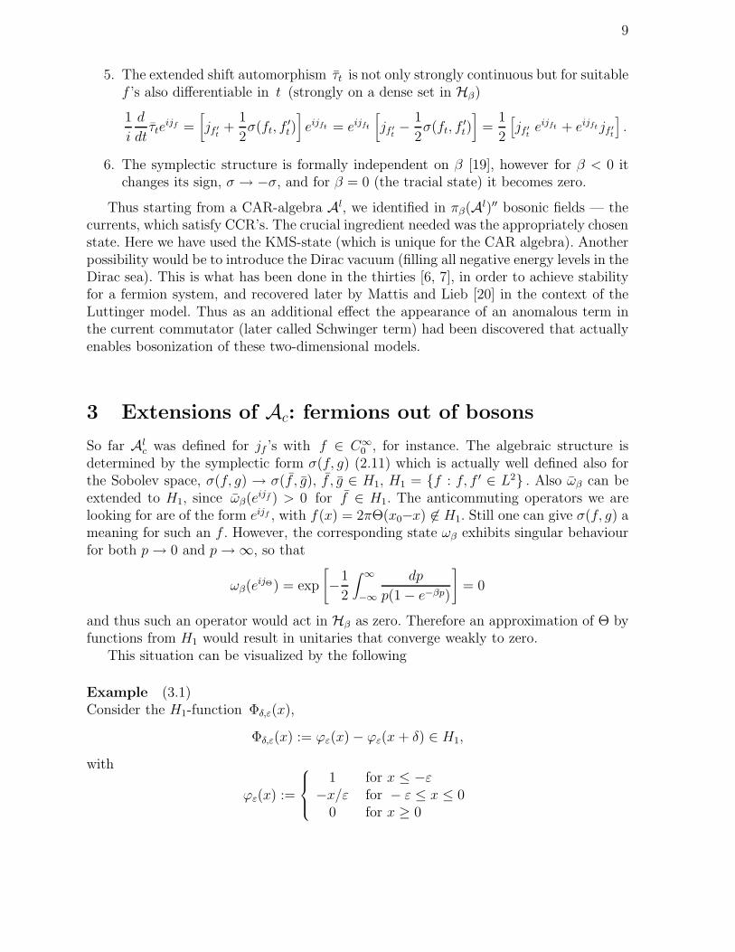
6. The symplectic structure is formally independent on β [19], however for β < 0 itchanges its sign, σ → −σ, and for β = 0 (the tracial state) it becomes zero.

Thus starting from a CAR-algebra Al, we identified in πβ(Al)′′ bosonic fields — thecurrents, which satisfy CCR’s. The crucial ingredient needed was the appropriately chosenstate. Here we have used the KMS-state (which is unique for the CAR algebra). Anotherpossibility would be to introduce the Dirac vacuum (filling all negative energy levels in theDirac sea). This is what has been done in the thirties [6, 7], in order to achieve stabilityfor a fermion system, and recovered later by Mattis and Lieb [20] in the context of theLuttinger model. Thus as an additional effect the appearance of an anomalous term inthe current commutator (later called Schwinger term) had been discovered that actuallyenables bosonization of these two-dimensional models.

3 Extensions of Ac: fermions out of bosons

So far Alc was defined for jf ’s with f ∈ C∞

0 , for instance. The algebraic structure isdetermined by the symplectic form σ(f, g) (2.11) which is actually well defined also forthe Sobolev space, σ(f, g) → σ(f , g), f , g ∈ H1, H1 = f : f, f ′ ∈ L2 . Also ωβ can beextended to H1, since ωβ(eijf ) > 0 for f ∈ H1. The anticommuting operators we arelooking for are of the form eijf , with f(x) = 2πΘ(x0−x) 6∈ H1. Still one can give σ(f, g) ameaning for such an f . However, the corresponding state ωβ exhibits singular behaviourfor both p→ 0 and p→∞, so that

ωβ(eijΘ) = exp

[−1

2

∫ ∞

−∞

dp

p(1− e−βp)

]= 0

and thus such an operator would act in Hβ as zero. Therefore an approximation of Θ byfunctions from H1 would result in unitaries that converge weakly to zero.

This situation can be visualized by the following

Example (3.1)Consider the H1-function Φδ,ε(x),

Φδ,ε(x) := ϕε(x)− ϕε(x+ δ) ∈ H1,

with

ϕε(x) :=

1 for x ≤ −ε−x/ε for − ε ≤ x ≤ 0

0 for x ≥ 0

10

as an approximation to the step function,

limδ→∞

ε→0

Φδ,ε(x) = Θ(x).

Then

Φδ,ε(p) =1− eipε

εp2(1− eipδ)

and

‖Φδ,ε‖2β =∫ ∞

−∞

dp

2π

p

1− e−βp|Φ(p)|2 = 16

∫ ∞

−∞

dp

2π

p

1− e−βp

sin2 pε/2

ε2p4sin2 pδ/2,

‖Φ‖2β ≥ c∫ 1/δ

0dp δ2 = cδ

for β/δ, ε/δ ≪ 1 and c a constant. Thus for δ →∞ , ‖Φδ‖β →∞. Also ‖Φδ − f‖β →∞since

‖Φδ − f‖β ≥ ‖Φδ‖β − ‖f‖β →∞ ∀ ‖f‖β <∞and thus

|〈Ω|e−ijf eijΦδ |Ω〉| = e−12‖Φδ−f‖2

β → 0.

But eijf |Ω〉, ‖f‖β < ∞, is total in Hβ and thus eijΦδ |Ω〉 and therefore eijΦδ goes weaklyto zero.

However the automorphism

eijf → e−ijΦδ eijf eijΦδ = eiσ(Φδ ,f)eijf

converges since

σ(f,Φδ) = − 1

2πε

(∫ 0

−ε−∫ −δ

−ε−δ

)dx f(x)

δ→∞−→ − 1

2πε

∫ 0

−εdx f(x)

ε→0−→ − 1

2πf(0).

The divergence of ‖Φδ,ε‖ is related to the well-known infrared problem of the masslessscalar field in (1+1) dimensions and various remedies have been proposed [21]. We takeit as a sign that one should enlarge Al

c to some Alc and work in the Hilbert space

H generated by Alc on the natural extension of the state. Thus we add to Al

c theidealized element ei2πjϕε = Uπ and keep σ and ωβ as before. Equivalently we take the

automorphism γ generated by Uπ and consider the crossed product Alc = Al

c

γ⊲⊳ Z .

There is a natural extension ω to Alc and a natural isomorphism of H and Al

c|Ω〉. HereH is the countable orthogonal sum of sectors with n particles created by Uπ. Thus,

〈Ω|eijfUπ|Ω〉 = 0 (3.2)

means that Uπ leads to the one-particle sector, in general

〈Ω|U∗nπ eijfUm

π |Ω〉 = δnm ωβ(γn eijf ).

11

The quasifree automorphisms on Alc (e.g. τt) can be naturally extended to Al

c ,τt Uπ = eiπjϕε,t , ϕε,t(x) = ϕε(x+ t) and since ϕε − ϕε,t ∈ H1 ∀ t, this does notlead out of Al

c.Uπ has some features of a fermionic field since

σ(ϕε, τtϕε) = −σ(ϕε, τ−tϕε) =1

4π

1 for t > ε

2tε− t2

ε2 for 0 ≤ t ≤ ε. (3.3)

More generally we could define Uα = ei√

2παjϕε and get from (3.3) with

sgn(t) = Θ(t)−Θ(−t) =

1 for t > 00 for t = 0−1 for t < 0.

Proposition (3.4)

UατtUα = τt(Uα)Uα ei α sgn(t)/2,

U∗ατtUα = τt(Uα)U∗

α ei α sgn(t)/2 ∀ |t| > ε.

Remark (3.5)We note a striking difference between the general case of anyon statistics and the twoparticular cases — Bose (α = 2 · 2nπ) or Fermi (α = 2(2n+ 1)π) statistics. Only in thelatter two cases parity P (2.12:4) is an automorphism of the extended algebra gener-ated through Uα. Thus P which was destroyed in Al

c is now recovered for two subalgebras.

The particle sectors are orthogonal in any case

〈Ω|U∗nα e

ijfUmα |Ω〉 = 0 ∀ n 6= m, f ∈ H1.

Furthermore, sectors with different statistics are orthogonal 〈Ω|U∗αUα′ |Ω〉 = 0, α 6= α′,

thus if we adjoin Uα, ∀α ∈ R+, Hβ becomes nonseparable.Next we want to get rid of the ultraviolet cut-off and let ε go to zero. Proceeding the

same way we can extend σ and τt but keeping ω the sectors abound. The reason is that

ϕεε→0−→ Θ(x) and

‖Θ−Θt‖2 =∫ ∞

−∞

dp p

1− e−βp

|1− eitp|2p2

is finite near p = 0 but diverges logarithmically for p→∞. This means that eijfeijΘ |Ω〉,f ∈ H1 gives a sector where one of these particles (fermions, bosons or anyons) is at thepoint x = 0 and is orthogonal to eijfeijΘt |Ω〉 ∀ t 6= 0. Thus the total Hilbert space is notseparable and the shift τt is not even weakly continuous, so there is no chance to makesense of d

dtτte

ijΘ .So far, only one chiral component has been considered. When both chiralities are

present, no significant changes arise in the construction described. The only point de-manding for some care is the anticommutativity between left- and right- moving fermions,

12

which asks for an even larger extension of the current algebra by extending its test–functions space.

So, the Weyl algebra Ac = Arc ⊗Al

c is now generated by the unitaries

W (fr, fl) = ei∫

(fr(x)jr(x)+fl(x)jl(x))dx,

with σ(fl, gl) given by (2.11) and σ(fr, gr) = −σ(fl, gl). The minimal extension of Ac isthen obtained by adding two idealized elements,

U lπ := W (cl, 2π(1− ϕε)) and U r

π := W (2πϕε, cr)

cl − cr = (2k + 1)π, k ∈ Z (e.g. cr = π/2 = −cl)They generate for ε→ 0 (not inner) automorphisms of Ac

U r(l)π : γr(l)W (fr, fl) = eifr(l)(0) e

i4

∫∞

−∞f ′

r(l)(y)dy

W (fr, fl)

in which for the two subalgebras W (f , f) and W (f ,−f), f ∈ Do ⊂ C∞o , the vectorand axial gauge transformations can easily be traced back.

In addition to the obvious replacement of (3.4), also the following relation holds

U r(∗)π U l

π = −U lπ U

r(∗)π .

Thus we can identify the chiral components of the fermion field with the so constructedunitaries

ψr(x) = limε→0

exp i2π∫ ∞

−∞ϕε(y − x)jr(x′)dx′ ± i

π

2

∫ ∞

−∞jl(x

′)dx′

ψl(x) = limε→0

exp ∓iπ2

∫ ∞

−∞jr(x

′)dx′ + i2π∫ ∞

−∞ϕε(x− y)jl(x′)dx′

(3.6)

In general, we could define an extension of the algebra Ac through the abstractelements U r(l)

α

U rα := W

(√2παϕε,

1

2

√πα

2

)

U lα := W

(−1

2

√πα

2,√

2πα (1− ϕε))

Propositon (3.4) extends also for the non-chiral model generalization. As expected,admitting arbitrary values for α, we get a very rich field structure where definite statisticbehaviour is preserved only within a given field class (fixed value of α), so that evendifferent fermions (with different “2 x odd” values of α) do not anticommute but insteadfollow the general fractional statistics law.

13

4 Anyon fields in πω(Ac)′′

Next we shall use another ultraviolet limit to construct local fields which obey someanyon statistics. Of course quantities like

[Ψ∗(x),Ψ(x′)]α := Ψ∗(x)Ψ(x′)ei 2π−α4

sgn(x′−x) + Ψ(x′)Ψ∗(x)e−i 2π−α4

sgn(x′−x) = δα(x−x′)

will only be operator valued distributions and have to be smeared to give operators.Furthermore in this limit the unitaries we used so far have to be renormalized so that thedistribution δα(x−x′) (which should be localized at a point and for certain values of α issupposed to coincide with the ordinary δ-function) gets a factor 1 in front. A candidatefor Ψ(x) will be

Ψ(x) := limε→0

nα(ε) exp[i√

2πα∫ ∞

−∞dy ϕε(x− y)j(y)

]

with ϕε from (3.1) and nα(ε) a suitably chosen normalization. With the shorthandϕε,x(y) = ϕε(x− y) and α =

√2πα we can write

Ψ∗ε(x)Ψε(x

′) = exp i 2πασ(ϕε,x, ϕε,x′) expiα jϕε,x′−ϕε,x

,

Ψε(x′)Ψ∗

ε(x) = exp −i 2πα σ(ϕε,x, ϕε,x′) expi α jϕε,x′−ϕε,x

.

We had in (3.3)

4πσ(ϕε,x, ϕε,x′) = sgn(x− x′)

Θ(|x− x′| − ε) + Θ(ε− |x− x′|)(x− x′)2

ε2

=: sgn(x− x′)Dε(x− x′)and thus

[Ψ∗ε(x),Ψε(x

′)]α = 2nα(ε)2 cos[sgn(x− x′)

(π

2− α

4(1−Dε(x− x′))

)]exp

iαjϕε,x′−ϕε,x

.

Note that for |x− x′| ≥ ε the argument of the cos becomes ±π/2, so the α–commutatorvanishes, in agreement with (3.4). To manufacture a δ-function for |x − x′| ≤ ε we notethat cos(...) > 0 and ωβ(eiαj) > 0, so we have to choose nα(ε) such that

2n2α(ε)ε

∫ 1

−1dδ cos

(π

2− α

4(1− δ2)

)· ωβ

(exp

iαjϕε,x−εδ−ϕε,x

)= 1

and to verify that for ε → 0+ [., .]α converges strongly to a c-number. For the latter tobe finite we have to smear Ψ(x) with L2-functions g and h:

∫dxdx′g∗(x)h(x′)[Ψ∗

ε(x),Ψε(x′)]α =

∫dxdx′g∗(x)h(x′)2nα(ε)2 cos( ) exp

iαjϕε,x′−ϕε,x

.

14

This converges strongly to 〈g|h〉 if for ε→ 0+

⟨exp

−iαjϕε,x′−ϕε,x

exp

iαjϕε,y′−ϕε,y

⟩

β−⟨exp

−iαjϕε,x′−ϕε,x

⟩

β

⟨exp

iαjϕε,y′−ϕε,y

⟩

β→ 0

for almost all x, x′, y, y′. Now

〈e−ijaeijb〉β = 〈e−ija〉β〈eijb〉β exp

[∫ ∞

−∞

dp p

1− eβpa(−p)b(p)

].

In our case this last factor is

∫ ∞

−∞

dp p

1− e−βp

|1− eipε|2ε2p4

(eipx − eipx′

)(e−ipy − e−ipy′

) =

=∫ ∞

−∞

dp 2(1− cos p)

p3(1− e−βp/ε)(eipx/ε − eipx′/ε)(e−ipy/ε − e−ipy′/ε).

For fixed β 6= 0 and almost all x, x′, y, y′ this converges to zero for ε → 0 by Riemann-Lebesgue. Thus a δ-type distribution is recognized, however the particular structure ofthe singularity we shall discuss later on, already on the basis of the state.

In the same way one sees that expiαjϕε,x+ϕε,x′

converges strongly to zero and that

the Ψε,g are a strong Cauchy sequence for ε→ 0. To summarize we state

Theorem (4.1)Ψε,g converges strongly for ε→ 0 to an operator Ψg which for α = 2π satisfies

[Ψ∗g,Ψh]+ = 〈g|h〉, [Ψg,Ψh]+ = 0.

If supp g < supp h,

Ψ∗gΨh e

i 2π−α4 + ΨhΨ

∗g e

−i 2π−α4 = 0 ∀α.

Furthermore we have to verify the claim (1.5) that also for Ψg the current jf inducesthe local gauge transformation g(x)→ e2iαf(x)g(x). For finite ε we have

eijf Ψε,ge−ijf = Ψε,ei2πασ(f,ϕε)g

and for ε→ 0+ we get σ(f, ϕε)→ 12πf(0) , so that σ(f, τxϕε) = 1

2πf(x).

To conclude we investigate the status of the “Urgleichung” in our construction. It isclear that the product of operator valued distributions on the r.h.s. can assume a meaningonly by a definite limiting prescription. Formally it would be

Ψ(x)Ψ∗(x)Ψ(x) = [Ψ(x),Ψ∗(x)]+Ψ(x)−Ψ∗(x)Ψ(x)2 = δ(0)Ψ(x)− 0.

From (2.12:5) we know

1

i

∂

∂xΨε(x) =

√2πα

2[(x),Ψε(x)]+, (x) =

1

ε

∫ x

x−εdy j(y).

15

Using

jϕ′eijφ =1

i

∂

∂αei α

2σ(ϕ′,ϕ)eijϕ+αϕ′

∣∣∣∣∣α=0

one can verify that the limit ε → 0+ exists for the expectation value with a total set ofvectors and thus gives densely defined (not closable) quadratic forms. They do not leadto operators but we know from (2.7), (2.8) that they define operator valued distributionsfor test functions from H1. Thus one could say that in the sense of operator valueddistributions the Urgleichung holds

1

i

∂

∂xΨ(x) =

√2πα

2[j(x),Ψ(x)]+. (4.2)

The remarkable point is that the coupling constant λ in (1.1) is related to the statisticsparameter α. For fermions one has a solution only for λ =

√2π. Of course one could for

any λ enforce fermi statistics by renormalizing the bare fermion field ψ →√Z ψ, j → Zj

with a suitable Z(λ) but this just means pushing factors around. Alternatively one could

extend Ac by adding ei√

2πα jϕε , for all α ∈ R+. Then one gets in Hω uncountably manyorthogonal sectors, one for each α, and in each sector a different Urgleichung holds.Thus different anyons live in orthogonal Hilbert spaces and ei

√2πα jϕε is not even weakly

continuous in α. If α is tied to λ it is clear that an expansion in λ is doomed to failureand will never reveal the true structure of the theory.

5 Correlation functions in a KMS-state

In terms of distributions, the τ -KMS-state ωβ over Al reads

〈ψ∗(x)ψ(x′)〉β =

∞∫

−∞dp

e−ip(x−x′)

2π (1 + eβp)(5.1)

= − 1

2π

∞∑

n=−∞

(−1)n

i(x− x′ + iε)− nβ

It can be also represented in a form that makes the thermal contributions explicit

〈ψ∗(x)ψ(x′)〉β =i(x− x′)

π

∞∑

n=1

(−1)n

(x− x′)2 + n2β2− 1

2π[i(x− x′)− ε]or, for a better comparison with the dressed-fermion correlators, as

〈ψ∗(x)ψ(x′)〉β =i

2β sinh π(x−x′+iε)β

, (5.2)

respectively

〈ψ(x′)ψ∗(x)〉β = − i

2β sinh π(x−x′−iε)β

. (5.3)

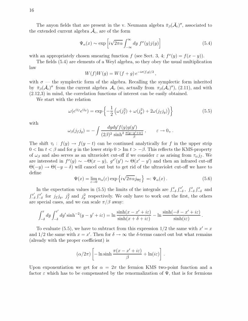
16

The anyon fields that are present in the v. Neumann algebra πβ(Ac)′′, associated to

the extended current algebra Ac, are of the form

Ψα(x) ∼ exp[i√

2πα∫ ∞

−∞dy fx(y)j(y)

](5.4)

with an appropriately chosen smearing function f (see Sect. 3, 4; fx(y) = f(x− y)).The fields (5.4) are elements of a Weyl algebra, so they obey the usual multiplication

lawW (f)W (g) = W (f + g) e−iσ(f,g)/2 ,

with σ — the symplectic form of the algebra. Recalling the symplectic form inheritedby πβ(Ac)

′′ from the current algebra Ac (so, actually from πβ(Ac)′′), (2.11), and with

(2.12,3) in mind, the correlation functions of interest can be easily obtained.We start with the relation

ω(eijfeijg) = exp−1

2

(ω(j2

f) + ω(j2g ) + 2ω(jfjg)

)(5.5)

with

ωβ(jf jg) = −∫ dydy′f(y)g(y′)

(2β)2 sinh2 π(y−y′+iε)β

, ε→ 0+ .

The shift τt : f(y) → f(y − t) can be continued analytically for f in the upper strip0 < Im t < β and for g in the lower strip 0 > Im t > −β. This reflects the KMS-propertyof ωβ and also serves as an ultraviolet cut-off if we consider ε as arising from τiεjf . Weare interested in fx(y) ∼ −Θ(x − y), gx′

(y′) ∼ Θ(x′ − y′) and then an infrared cut-offΘ(−y) → Θ(−y − δ) will cancel out but to get rid of the ultraviolet cut-off we have todefine

Ψ(x) = limε→0

nα(ε) expi√

2παjΘxε

=: Ψα(x) . (5.6)

In the expectation values in (5.5) the limits of the integrals are∫ x−δ

∫ x′

−δ ,∫ x−δ

∫ x−δ and

∫ x′

−δ

∫ x′

−δ for jf jg, j2f and j2

g respectively. We only have to work out the first, the othersare special cases, and we can scale π/β away:

∫ x

−δdy∫ x′

−δdy′ sinh−2(y − y′ + iε) = ln

sinh(x− x′ + iε)

sinh(x+ δ + iε)− ln

sinh(−δ − x′ + iε)

sinh(iε).

To evaluate (5.5), we have to subtract from this expression 1/2 the same with x′ = xand 1/2 the same with x = x′. Then for δ →∞ the δ-terms cancel out but what remains(already with the proper coefficient) is

(α/2π)

[− ln sinh

π(x− x′ + iε)

β+ ln(iε)

].

Upon exponentiation we get for α = 2π the fermion KMS two-point function and afactor ε which has to be compensated by the renormalization of Ψ, that is for fermions

17

the renormalization parameter should be n2π(ε) = (2πε)−1/2 and for the general case ofan arbitrary α : nα(ε) = (2πε)−α/4π.

For all α’s the two-point function (for x 6= x′ and β = π)

〈Ψ∗α(x)Ψα(x′)〉β = 〈Ψα(x)Ψ∗

α(x′)〉β =

(i

2β sinh(x− x′)

)α/2π

=: Sα(x− x′) (5.7)

has the desired properties

1. Hermiticity:

S∗α(x) = Sα(−x) ⇐⇒ 〈Ψ∗

α(x)Ψα(x′)〉∗β = 〈Ψ∗α(x′)Ψα(x)〉β ;

2. α-commutativity:

Sα(−x) = eiα/2Sα(x) ⇐⇒ 〈Ψα(x′)Ψ∗α(x)〉β = eiα/2〈Ψ∗

α(x)Ψα(x′)〉β ;

3. KMS-property:

Sα(x) = Sα(−x+ iπ) ⇐⇒ 〈Ψ∗α(x)Ψα(x′)〉β = 〈Ψα(x′)Ψ∗

α(x+ iπ)〉β .

Remark

If the deformation parameter exp iα/2 = q 6∈ S1 but instead q ∈ (−1, 1) then there areno KMS-states since there do not exist even translation invariant states [22].

For α = 2π Eq.(5.7) reads

〈Ψ∗2π(x)Ψ2π(x′)〉β = lim

ε→0+

i

2β sinh π(x−x′+iε)β

. (5.8)

For f(y)→ Θ(x− y), g(y′)→ −Θ(x′ − y′) nothing changes so we verify the realtion(5.2) ↔ (5.3),

〈Ψ∗2π(x)Ψ2π(x′)〉β = 〈Ψ2π(x)Ψ∗

2π(x′)〉β .For α = 4π we get like for the j’s

〈Ψ∗4π(x)Ψ4π(x′)〉β = − 1

(2β sinh π(x−x′+iε)

β

)2 , (5.9)

whereas for α = 6π we get a different kind of fermions

〈Ψ∗6π(x)Ψ6π(x′)〉β = − i

(2β sinh π(x−x′+iε)

β

)3 . (5.10)

They are not canonical fields since

−[Ψ∗6π(x),Ψ6π(x′)]α = [Ψ∗

6π(x),Ψ6π(x′)]+ = − 1

8π2

(δ′′(x− x′)− π2

β2δ(x− x′)

).

18

This shows that local anticommutativity alone does not guarantee the uniqueness of theKMS-state, one needs in addition the CAR-relations. The Ψα’s, α ∈ (2N+1)π , describean infinity of inequivalent fermions.

For the thermal expectation of the α-commutator one finds

ωβ([Ψ∗(x),Ψ(x′)]α) = −i

− 1

2β sinh π(x−x′+iε)β

α/2π

+ i

− 1

2β sinh π(x−x′−iε)β

α/2π

(5.11)

and for ε→ 0 a distribution is obtained where only the leading singularity is temperatureindependant, namely

limε→0

(1

x− x′ − iε

)α/2π

−(

1

x− x′ + iε

)α/2π

= ?

We shall not attempt to make sense of the “canonical” anyon commutators. Anotherinteresting topic — the higher correlation functions, since the limiting procedures involvedmight influence their properties, we shall also discuss separately [23].

6 Internal symmetries

We shall briefly discuss what happens in the the case of a fermion multiplet. Then,

ψ∗i (x), ψk(y) = δik δ(x− y), i = 1, 2, ..., N

The CAR-algebra so defined posesses an obvious U(N) symmetry

ψ −→ U ψ, U ∈ U(N)

In analogy with the previous case we construct quadratic forms jk(x) = ψ∗k(x)ψk(x)

which satisfy anomalous commutation relations:

[jk(x), jm(y)] = − i

2πδkmδ

′(x− y) (6.1)

and give rise to operators jfk=∫jk(x)fk(x)dx, f ∈ H1.

Denote the corresponding Weyl operators with W (f1, ..., fN)

W (f1, ..., fN) := expiN∑

n=1

jfn

The current algebra (6.1) has a (global) O(N) symmetry,

j →Mj = j′, M ∈ O(N) (6.2)

19

Genuine anticommuting fields can now be identified in an extension of the currentalgebra quite similar to the one for the non-chiral one-colour case. More precisely, wehave to allow for the existence in the new algebra of the following elements

Uπk= e

i2π∞∫

−∞

ϕ(x−x′)jk(x′)dx′+i

N∑

n=1 ,n 6=k

cn

∞∫

−∞jn(x′)dx′

=: ψk(x),

ck ∈ R, ck − cn = (2l + 1)π, l ∈ Z, ∀k, n . (6.3)

For the elements so defined the following relation holds

ψ∗k(x)ψl(y) = ψl(y)ψ

∗k(x)e

−iπ δkl sgn(y−x) e−i(1−δkl)(ck−cl)

which would then lead (after an appropriate renormalisation) to the desired CAR’s.How should one consider the element, obtained through the same ansatz, but after a

transformation (6.2) of the currents, i.e.

ψ′k(x) = e

i2π∫ x

−∞Mkljl(x

′)dx′+(...)(6.4)

Has it something to do with the U(N)-transformed fermion ψ′k, i.e.

ei2π∫ x

−∞Mkljl(x

′)dx′ ?←→ Uklψl(x)

What one notices is that the O(N)-transformation, being (of course) an isomorphismof the algebra Ac , is no longer an automorphism of the total algebra.

In such a symmetry nonpreservation a major limitation of the usual bosonizationscheme (with non-local fermi fields, [24, 25]) has been recognized, e.g. the O(N) symmetryof a free scalar theory with N fields, which emerges upon bosonization of a theory withN free Dirac fields with U(N) × U(N) chiral invariance, does not correspond to anysubgroup of the fermion symmetry group [26]. The bosonization scheme proposed thereinpreserves all symmetries through the passage from one formulation to the other. However,this does not concern the complete cycle where, as we have seen, symmetries may be(actually, necessarily are) spontaneously destroyed.

We are faced with the similar situation also for the U -invariance we mentioned at thebeginning. Here, e.g. for U(1) , so

ψk(x)→ eiαψk(x)

we get

ψ′k(x) = eiαe

i2π∫ x

−∞jk(x′)dx′

= ei2π∫ x

−∞j′k(x′)dx′

with

j′k(x′) = jk(x

′) +1

2πα(x′), α(k) :

∫ x

−∞α(x′) = α(x)

In the local case this still remains an automorphism of the extended algebra, whichis in agreement with the very idea of the construction presented, while for a global

20

transformation this is no longer the case, so for the total algebra so constructed there isno global U(1) symmetry present.

However, on the passage from the CAR-algebra A to the current algebra Ac con-tained in the v.Neumann algebra πβ(A)′′ the parity has been broken, but also as anisomorphism of Ac .

Thus we are in a situation in which a particular (physically motivated) extensionAc, of the algebra of observables (the current algebra Ac ) is constructed, Ac ⊃ Ac,such that 6 ∃β ∈ Aut Ac : β|A = α for some α ∈ Aut Ac . This phenomenon we callsymmetry destruction. It is related to the spontaneous collapse of a symmetry, discussedby Buchholz and Ojima in the context of supersymmetry [16] and is seen to be a fieldeffect since in contrast to the spontaneous symmetry breaking [17], it cannot occur in afinite-dimensional Hilbert space.

7 Concluding remarks

To summarize we gave a precise meaning to eq.(1.2a,b,c) by starting with bare fermions,A = CAR(R). The shift τt is an automorphism of A which has KMS-states ωβ andassociated representations πβ. In πβ(A)′′ one finds bosonic modes Ac with an algebraicstructure independent on β. Taking the crossed product with an outer automorphism ofAc or equivalently augmenting Ac by an unitary operator to Ac we discover in πβ(Ac)

′′

anyonic modes which satisfy the Urgleichung in a distributional sense. For special valuesof λ they are dressed fermions distinct from the bare ones. From the algebraic inclusionsCAR(bare) ⊂ πβ(A)′′ ⊃ Ac ⊂ Ac ⊂ πβ(Ac)

′′ ⊃ CAR(dressed) one concludes that in ourmodel it cannot be decided whether fermions or bosons are more fundamental. One canconstruct the dressed fermions either from bare fermions or directly from the currentalgebra. Also the correlation functions in the temperature state in both cases coincidethat is in agreement with the uniqueness of the τ -KMS state over a CAR algebra (τ beingthe shift automorphism). The corresponding anyonic two-point function evaluated for thespecial case of a scalar field reproduces the recent result due to Borchers and Yngvason.

Acknowledgements

The authors are grateful to H. Narnhofer, R. Haag and J. Yngvason for helpfuldiscussions on the subject of this paper.

N.I. acknowledges the financial support from the “Fonds zur Forderung der wis-senschaftlichen Forschung in Osterreich” under grant P11287–PHY and the hospitalityat the Institute for Theoretical Physics of University of Vienna.

21

Appendix The field algebra as a crossed product

The idea that the crossed product C∗-algebra extension is the tool that makes possibleconstruction of fermions (so, unobservable fields) from the observable algebra has beenfirst stated in [27]. There, the problem of obtaining different field groups has been shownto amount to construction of extensions of the observable algebra by the group duals.Explicitly, crossed products of C∗-algebras by semigroups of endomorphisms have beenintroduced when proving the existence of a compact global gauge group in particle physicsgiven only the local observables [28]. Also in the structural analysis of the symmetriesin the algebraic QFT [5] extendibility of automorphisms from a unital C∗-algebra to itscrossed product by a compact group dual becomes of importance since it provides ananalysis of the symmetry breaking [17] and in the case of a broken symmetry allows forconcrete conlusions for the vacuum degeneracy [29].

The reason why a relatively complicated object — crossed product over a speciallydirected symmetric monoidal subcategory EndA of unital endomorphisms of the observ-able algebra A, is involved in considerations in [29] is that in general, non-Abelian gaugegroups are envisaged. For the Abelian group U(1) a significant simplification is possiblesince its dual is also a group — the group Z. On the other hand, even in this simplecase the problem of describing the local gauge transformations remains open. Thereforein the Abelian case consideration of crossed products over a discrete group offers botha realistic framework and reasonable simplification for the analysis of the resulting fieldalgebra. We shall briefly outline the general construction for this case, for more detailssee [13].

We start with the CCR algebra A(V0, σ) over the real symplectic space V0 withsymplectic form σ, Eq.(2.11), generated by the unitaries W (f), f ∈ V0 with

W (f1)W (f2) = e−iσ(f1,f2)/2W (f1 + f2), W (f)∗ = W (−f) = W (f)−1.

Instead of the canonical extension A(V, σ), V0 ⊂ V [12], we want to construct anotheralgebra F , such that CCR(V0) ⊂ F ⊂ CCR(V) and we choose V0 = C∞

0 , V = ∂−1C∞0 .

Any free (not inner) automorphism α, α ∈ AutA defines a crossed product F = A α⊲⊳ Z .

This may be thought as (see [30]) adding to the initial algebra A a single unitary operatorU together with all its powers, so that one can formally write F =

∑nAUn , with U

implementing the automorphism α in A, αA = U AU∗, ∀A ∈ A. Operator U should bethought of as a charge-creating operator and F is the minimal extension — an importantpoint in comparison to the canonical extension which we find superfluous especially whenquestions about statistical behaviour and time evolution are to be discussed. With thechoice

αW (f) = eiσ(g,f)W (f), g ∈ V\V0, V0 ⊂ V (A.1)

and identifying U = W (g) , F is in a natural way a subalgebra of CCR(V).If we take for A the current algebra Ac and for U — the idealized element Uπ to

be added to it, we find an obvious correspondence between the functional picture fromSec.3 and the crossed product construction. However, in the latter there is an additional

22

structure present which makes it in some cases favourable. Writing an element F ∈ Fas F =

∑nAnU

n, An ∈ A , we see that it is convenient to consider F as an infinitevector space with Un as its basic unit vectors and An =: (F )n as components of F . Thealgebraic structure of F implies that multiplication in this space is not componentwisebut instead

(F.G)m =∑

n

Fn αnGm−n.

Given a quasifree automorphism ρ ∈ AutA, it can be extended to F if and only ifthe related automorphism γρ = ραρ−1α−1 is inner for A. Since γρ is implemented byW (gρ − g), this is nothing else but demanding that gρ − g ∈ V0 and this is exactly thesame requirement as in the functional picture. This appears to be the case for the spacetranslations and also for the time evolution, but in the absence of long-range forces [13].

Also a state ω(.) over A together with the representation πω associated with itthrough the GNS-construction can be extended to F . The representation space of Fcan be regarded as a direct sum of charge-n subspaces, each of them being associatedwith a state ω α−n and with H0, the representation space of A, naturally imbeddedin it. Since ω is irreducible and ω α−n not normal with respect to it, the extension ofthe state over A to a state over F is uniquely determined by the expectation value with|Ω0〉 = |ω〉 in this representation

〈Ωk|W ∗(f)W (h)W (f)|Ωn〉 = δkn e−iσ(f+ng,h)ω(W (h))

where Uk|Ω〉 := |Ωk〉, 〈Ωk|Ωn〉 = δkn . This states nothing but orthogonality of the differ-ent charge sectors, the same as in the functional description, Eq.(3.2).

In the crossed product gauge automorphism is naturally defined with

γν Un = e2πiνnUn, γν W (f) = W (f) . (A.2)

Thus for the representation πΩ one finds

γν

(|F (f)(k)〉

)= γν (W (f)|Ωk〉) = e2πiνkW (f)|Ωk〉,

that justifies interpretation of the vectors |F (f)(k)〉 as belonging to the charge-k subspace.However, A is a subalgebra of F for the gauge group T = [0, 1), while it is a subalgebraof CAR for the gauge group T ⊗ R. Thus the crossed product algebra so constructed,being really a Fermi algebra, does not coincide with CAR but is only contained in it. Inother words, such a type of extension does not allow incorporation also of local gaugetransformations which are of main importance in QFT.

Therefore we need a generalization of the construction in [13] which would describealso the local gauge transformations. The most natural candidate for a structural auto-morphism would be

αgxW (f) = ei∑K

n=0f(n)(x)W (f). (A.3)

However, it turns out that only for n = 0 the crossed product algebra so obtained allowsfor extension of space translations as an automorphism of A — the minimal requirement

23

one should be able to meet. Already first derivative gives for the zero Fourier componentof the difference gxδ

− gx an expression of the type∫y−1δ(y)dy, so it drops out of C∞

0 .So, the automorphism of interest reads

αgxW (f) = eif(x)W (f) (A.4)

and can be interpreted as being implemented by W (gx) with gx = 2πΘ(x−y). Corre-spondingly, the operator we add to A through the crossed product is

Ux = ei2π∫ x

−∞j(y)dy

. (A.5)

Compared to [13] this means an enlargment of the test functions space not with a kinkbut with its limit — the sharp step function. In a distributional sense it still can beconsidered as an element of ∂−1V0 for some V0 since the derivative of gx has boundedzero Fourier component. Similarly, the extendibility condition for space translations isfound to be satisfied, gxδ

− gx ∈ V0 so that in the crossed product shifts are given by

τxδUx = Vxδ

Ux, Vxδ= W (gxδ

− gx). (A.6)

Note that shifts do not commute with the structural automorphism αgx , τxδαgxW (f) 6=

αgxτxδW (f). Since

σ(gx, gxδ) = −πsgn(δ), (A.7)

already the elements of the first class are anticommuting and we identify Ux =: ψ(x).Then (A.4) (after smearing with a function from C∞

0 ) is nothing else but (1.5), i.e. thestatement (or requirement) that currents generate local gauge transformations of the so–constructed field. Any scaling of the function which defines the structural automorphismαgx destroys relation (A.7) and fields obeying fractional statistics are obtained instead.This is effectively the same as adding to the algebra A the element Uα with α = 2πµ, µbeing the scaling parameter.

However, the crossed product offers one more interesting possibility: when for thesymplectic form in question instead of (A.7) (or its direct generalization σ(gx, gxδ

) =(2n + 1)π, n ∈ Z ) another relation takes place, σ(gx, gxδ

) = (2n + 1)/n2 for some fixedn ∈ Z, the crossed product acquires a zone structure, with 2nn–classes commuting,(2n + 1)–classes anticommuting and elements in the classes with numbers m ∈ Z/Zn

obeying an anyon statistics with parameter r =√

2n+ 1m/n . So, fields with differentstatistical behaviour are present in the same algebra, however the Hilbert space remainsseparable.

We want to emphasize that relation of the type ψ(x+δx) = Ux+δx may be misleading,the latter element exists in the crossed product only by Eq.(A.6), so that for the derivativeone finds

∂ψ(x)

∂x:= lim

δx→0

ψ(x+ δx)− ψ(x)

δx= lim

δx→0

1

δx(Vxδ

Ux − Ux) =

limδx→0

1

δx

(ei 2π δx j(x) − 1

)Ux = 2π i j(x)Ux =: 2π i j(x)ψ(x). (A.8)

24

This, together with (2.5) gives for the operators

iψf ′ = ψf jΘ′ . (A.9)

Note that in the crossed product, which can actually be considered as a left A-module,equations of motion (A.8), (A.9) appear (due to this reason) without an antisymmetriza-tion, which was the case with the functional realization, Eq.(4.2), but otherwise the resultis the same. Therefore the scaling sensitivity of the crossed product field algebra is an-other manifestation of the quantum “selection rule” for the value of λ in the Urgleichung(1.2c).

References

[1] T.D. Lee, Phys. Rev. 95, 1329 (1954).

[2] H. Bethe, Z. Physik 71, 205 (1931).

[3] W. Heisenberg, Z. Naturforsch. 9a, 292 (1954).

[4] W. Thirring, Ann. Phys. 3, 91 (1958).

[5] R. Haag, Local Quantum Physics (Springer, Berlin Heidelberg, 1993).

[6] P. Jordan, Z. Phys. 93, 464 (1935); 98, 759 (1936);99, 109 (1936).

[7] M. Born, N. Nagendra–Nath, Proc. Ind. Acad. Sci. 3, 318 (1936).

[8] G. Dell’Antonio, Y. Frischman, D. Zwanziger, Phys. Rev. D6, 988 (1972).

[9] S. Mandelstam, Phys. Rev. D11, 3026 (1975).

[10] A.L. Carey, S.N.M. Ruijsenaars, Acta Appl. Math. 10, 1 (1987).

[11] A.L. Carey, C.A. Hurst, D.M. O’Brien, J. Math. Phys. 24, 2212 (1983).

[12] F. Acerbi, G. Morchio, F. Strocchi, Lett. Math. Phys. 26 (1992) 13; 27, 1 (1993).

[13] N. Ilieva, H. Narnhofer, OAW Sitzungsber. II 205, 13 (1996).

[14] N. Ilieva, W. Thirring, Eur. Phys. J. C6, 705 (1999).

[15] H.J. Borchers, J. Yngvason, J. Math. Phys. 40, 601 (1999).

[16] D. Buchholz and I. Ojima, Nucl. Phys. B498, 228 (1997).

[17] H. Narnhofer, W. Thirring, Ann. Inst. Henri Poincare 70, 1 (1999).

25

[18] J. Schwinger, Phys. Rev. 128, 2425 (1962).

[19] H. Grosse, W. Maderner, C. Reitberger, in Generalized Symmetries in Physics, Eds.H.–D. Dobner, V. Dobrev, and A. Ushveridze (World Scientific, Singapore, 1994).

[20] D.C. Mattis and E. Lieb, J. Math. Phys. 6, 304 (1965).

[21] F. Strocchi, General Properties of QFT, Lecture Notes in Physics – vol.51 (WorldScientific, Singapore, 1993).

[22] H. Narnhofer, private communication.

[23] N. Ilieva, W. Thirring, in preparation.

[24] S. Coleman, Phys. Rev. D11, 2088 (1975).

[25] S. Mandelstam, Phys. Rev.D11, 3026 (1975).

[26] E. Witten, Commun. Math. Phys. 92, 455 (1984).

[27] S. Doplicher, R. Haag, J. Roberts, Commun. Math. Phys. 15, 173 (1969).

[28] S. Doplicher, J. Roberts, Ann. Math. 130, 75 (1989).

[29] D. Buchholz, S. Doplicher, R. Longo, J. Roberts, Commun. Math. Phys. 155, 123(1993).

[30] H. Araki, in On Klauder’s Path: A Field Trip, Eds. G. Emch, G. Hegerfeldt, L. Streit(World Scientific, Singapore, 1994), p.11.