Ae

La

b

a

ARRAA

KAUCSUS

1

(dWn(ivTtt2

w

(

0d

Landscape and Urban Planning 101 (2011) 43–51

Contents lists available at ScienceDirect

Landscape and Urban Planning

journa l homepage: www.e lsev ier .com/ locate / landurbplan

nuran species in urban landscapes: Relationships with biophysical, builtnvironment and socio-economic factors

isa T. Smallbonea,∗, Gary W. Lucka, Skye Wassensb

Institute for Land, Water and Society, Charles Sturt University, P.O. Box 789, Albury, NSW 2640, AustraliaInstitute for Land, Water and Society, Charles Sturt University, Locked Bag Wagga Wagga, NSW 2678, Australia

r t i c l e i n f o

rticle history:eceived 9 July 2010eceived in revised form 5 January 2011ccepted 7 January 2011vailable online 15 February 2011

eywords:mphibiansrbanisationonnectivityouth-eastern Australiarban wetlandsocioeconomics

a b s t r a c t

Urbanisation is a significant threatening process for amphibians, causing loss of habitat, altered hydrologyand increased mortality. Impacts operate at different spatial scales and consequences vary depending onthe sensitivity of individual species. Most studies of the impact of urbanisation on anurans have occurredin large metropolitan cities. There is a paucity of research in smaller urban settlements where the impactsof development may be less pronounced. We examined the richness and occurrence of anuran species inwetlands in regional towns in south-eastern Australia as a factor of natural and built features occurring atmultiple spatial scales, and the socio-economic characteristics of surrounding neighbourhoods. Anuranspecies richness declined with increasing isolation of wetlands and reduced cover of terrestrial vegetation.The occurrence of two wide-spread anuran species was negatively related to level of urban intensity andpositively related to neighbourhood vegetation cover, whereas the converse was true for a third commonspecies. Vegetation cover was greater in neighbourhoods with ‘higher’ socioeconomic status (e.g. more

disposable income). These less developed neighbourhoods occurred on the fringes of towns, often inelevated locations, and tended to support more anuran species. The level of urban intensity increasedcloser to town centres and more developed neighbourhoods with lower socio-economic status were oftenbuilt in low-lying areas where wetlands tend to form naturally. Yet, these neighbourhoods harbouredfew anuran species.

Our study suggests that careful planning of low-lying neighbourhoods near town centres and periurbanfring

neighbourhoods on town

. Introduction

Urbanisation is a key threatening process for amphibiansHamer and McDonnell, 2008), which have shown significanteclines globally (Blaustein and Kiesecker, 2002; McCallum, 2007;ilcox, 2006). Urbanisation can adversely affect anuran commu-

ities by increasing vehicle-related mortality and habitat isolationElzanowski et al., 2009; Lehtinen et al., 1999), and by modify-ng aquatic and terrestrial habitats, reducing water quality (e.g.ia polluted run-off) and changing water flows and infiltration.hese factors operate at different spatial scales and their impor-ance varies depending on the sensitivity of individual species and

he characteristics of the urban environment (Gagné and Fahrig,007; Mazerolle et al., 2005; Price et al., 2005).

At broad scales, road and dwelling density is strongly associatedith the level of modification to urban wetlands and can influence

∗ Corresponding author. Tel.: +61 2 6051 9902; fax: +61 2 6051 9897.E-mail addresses: lsmallbone@csu.edu.au (L.T. Smallbone), galuck@csu.edu.au

G.W. Luck), swassens@csu.edu.au (S. Wassens).

169-2046/$ – see front matter Crown Copyright © 2011 Published by Elsevier B.V. All rigoi:10.1016/j.landurbplan.2011.01.002

es is required to ensure anuran conservation in urban settlements.Crown Copyright © 2011 Published by Elsevier B.V. All rights reserved.

the movement of amphibians between suitable habitat (Hamerand McDonnell, 2008), and alter and increase stormwater runoff,negatively impacting tadpole growth and survival (Eigenbrodet al., 2008; Hartel et al., 2009; Parris, 2006). When roads intersectwetlands, they cause loss and fragmentation of habitat and canseparate natal ponds from important terrestrial and over-winterlocations (Pillsbury and Miller, 2008; Rubbo and Kiesecker, 2005).High density road networks are substantial barriers to amphibianmovement and habitat re-colonization, and increase the likelihoodof mortality (Drinnan, 2005; Ficetola and De Bernardi, 2004;Knutson et al., 1999; Price et al., 2005).

At smaller scales (e.g. individual ponds), habitat occupancycan be influenced by a range of factors including the complexityand cover of fringing and aquatic vegetation, presence of fish,hydrology, pond size, and water depth (Hamer and McDonnell,2008; Parris, 2006; Pillsbury and Miller, 2008). Many anurans

shelter in fringing vegetation during the day, which is importantfor protection from predators, regulating microclimates and pro-viding shelter for males during calling. The structure and type ofaquatic vegetation can determine the availability of anchor pointsfor egg masses, provide protection for tadpoles and contribute to

hts reserved.

44 L.T. Smallbone et al. / Landscape and Urban Planning 101 (2011) 43–51

ws m

taaaEnc2

ot(StwBofeerutisHucian

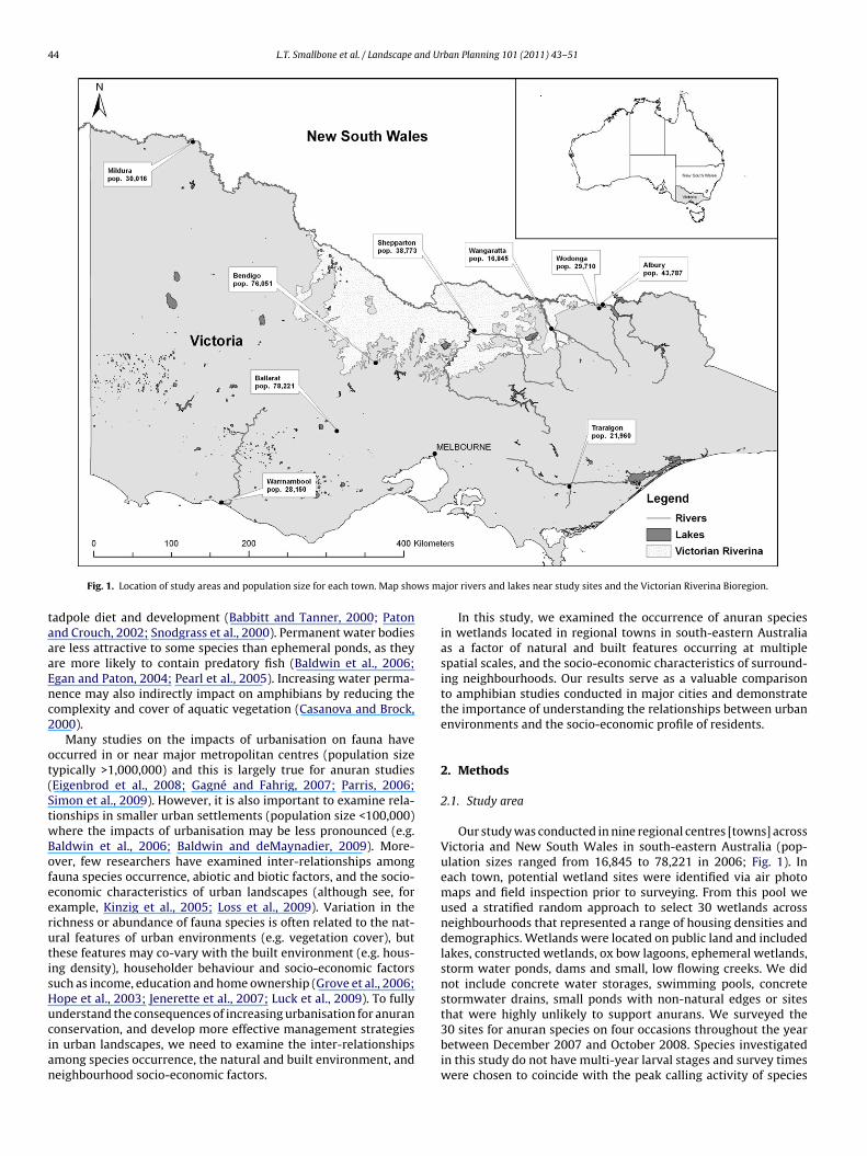
Fig. 1. Location of study areas and population size for each town. Map sho

adpole diet and development (Babbitt and Tanner, 2000; Patonnd Crouch, 2002; Snodgrass et al., 2000). Permanent water bodiesre less attractive to some species than ephemeral ponds, as theyre more likely to contain predatory fish (Baldwin et al., 2006;gan and Paton, 2004; Pearl et al., 2005). Increasing water perma-ence may also indirectly impact on amphibians by reducing theomplexity and cover of aquatic vegetation (Casanova and Brock,000).

Many studies on the impacts of urbanisation on fauna haveccurred in or near major metropolitan centres (population sizeypically >1,000,000) and this is largely true for anuran studiesEigenbrod et al., 2008; Gagné and Fahrig, 2007; Parris, 2006;imon et al., 2009). However, it is also important to examine rela-ionships in smaller urban settlements (population size <100,000)here the impacts of urbanisation may be less pronounced (e.g.aldwin et al., 2006; Baldwin and deMaynadier, 2009). More-ver, few researchers have examined inter-relationships amongauna species occurrence, abiotic and biotic factors, and the socio-conomic characteristics of urban landscapes (although see, forxample, Kinzig et al., 2005; Loss et al., 2009). Variation in theichness or abundance of fauna species is often related to the nat-ral features of urban environments (e.g. vegetation cover), buthese features may co-vary with the built environment (e.g. hous-ng density), householder behaviour and socio-economic factorsuch as income, education and home ownership (Grove et al., 2006;ope et al., 2003; Jenerette et al., 2007; Luck et al., 2009). To fully

nderstand the consequences of increasing urbanisation for anuranonservation, and develop more effective management strategiesn urban landscapes, we need to examine the inter-relationshipsmong species occurrence, the natural and built environment, andeighbourhood socio-economic factors.

ajor rivers and lakes near study sites and the Victorian Riverina Bioregion.

In this study, we examined the occurrence of anuran speciesin wetlands located in regional towns in south-eastern Australiaas a factor of natural and built features occurring at multiplespatial scales, and the socio-economic characteristics of surround-ing neighbourhoods. Our results serve as a valuable comparisonto amphibian studies conducted in major cities and demonstratethe importance of understanding the relationships between urbanenvironments and the socio-economic profile of residents.

2. Methods

2.1. Study area

Our study was conducted in nine regional centres [towns] acrossVictoria and New South Wales in south-eastern Australia (pop-ulation sizes ranged from 16,845 to 78,221 in 2006; Fig. 1). Ineach town, potential wetland sites were identified via air photomaps and field inspection prior to surveying. From this pool weused a stratified random approach to select 30 wetlands acrossneighbourhoods that represented a range of housing densities anddemographics. Wetlands were located on public land and includedlakes, constructed wetlands, ox bow lagoons, ephemeral wetlands,storm water ponds, dams and small, low flowing creeks. We didnot include concrete water storages, swimming pools, concretestormwater drains, small ponds with non-natural edges or sites

that were highly unlikely to support anurans. We surveyed the30 sites for anuran species on four occasions throughout the yearbetween December 2007 and October 2008. Species investigatedin this study do not have multi-year larval stages and survey timeswere chosen to coincide with the peak calling activity of species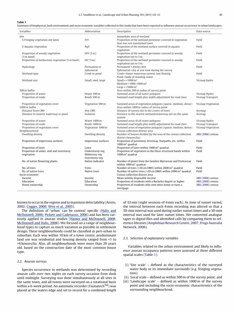

L.T. Smallbone et al. / Landscape and Urban Planning 101 (2011) 43–51 45

Table 1Summary of biophysical, built environment and socio-economic variables collected in this study that have been reported to influence anuran occurrence in urban landscapes.

Variables Abbreviation Description Data source

Site Immediate area of wetland% Fringing vegetation not lawn FrV Proportion of the wetland perimeter covered in vegetation

that was not maintained lawnField

% Aquatic vegetation AqV Proportion of the wetland surface covered in aquaticvegetation

Field

Proportion of woody vegetation(5 m band)

WV (5 m) Proportion of the wetland perimeter covered in woodyvegetation out to 5 m

Field

Proportion of herbaceous vegetation (5 m band) HV (5 m) Proportion of the wetland perimeter covered in woodyvegetation out to 5 m

Field

Hydrology Permanent orephemeral

Permanent = always wetEphemeral = dry at one time during the survey

Field

Wetland type Creek or pond Creek = linear waterway system, low flowingPond = body of standing water

Field

Wetland size Small, med, large Small = <1000 m2

Medium = 1000–5000 m2

Large = >5000 m2

Vicmap hydro

500 m buffer Area within 500 m radius of survey pointProportion of water Water 500 m Summed areas of all water polygons Vicmap HydroProportion of roads Roads 500 m Summed road length plus width adjustment for road class Vicmap Transport

Proportion of vegetation cover Vegetation 500 m Summed areas of vegetation polygons (sparse, medium, dense) Vicmap Vegetation1000 m buffer Area within 1000 m radius of survey point

Distance from CBD Dist CBD Distance of survey site to the centre of town ArcmapDistance to nearest waterway or pond Isolation Distance to the nearest wetland/waterway not on the same

systemArcmap

Proportion of water Water 1000 m Summed areas of all water polygons Vicmap HydroProportion of roads Roads 1000 m Summed road length plus width adjustment for road class Vicmap TransportProportion of vegetation cover Vegetation 1000 m Summed areas of vegetation polygons (sparse, medium, dense) Vicmap Vegetation

Neighbourhood Census collection district areaDwelling density Dwelling density Number of houses divided by the area of the census collection

district (houses/ha)ABS (2006) census

Proportion of impervious surfaces Impervious surfaces Proportion of pavement, driveway, footpaths, etc. within1000 m2 quadrat

Field

Proportion of lawn Lawn Proportion of lawn within 1000 m2 quadrat FieldProportion of under, mid and overstoreyvegetation

Understorey vegMidstorey vegOverstorey veg

Proportion of vegetation in the three structural bands within1000 m2 quadrat

Field

No. of native flowering plants Native indicator Number of plants from the families Myrtaceae and Proteaceaewithin 1000 m2 quadrat

Field

No. of trees Trees Number of trees (>20 cm DBH) within 2000 m2 quadrat FieldNo. of native trees Native trees Number of native trees (>20 cm DBH) within 2000 m2 quadrat Field

Socio-economic Census collection district areaIncome Income Mean weekly disposable income ABS (2006) censusEducation Education Proportion of residents with a Bachelor degree or higher ABS (2006) census

Propomortg

k2

MiMhdsl>ot

2

autwp

Home ownership Ownership

nown to occur in the regions and to maximise detectability (Anstis,002; Cogger, 2000; Weir et al., 2005).

The definition of ‘urban’ can be context specific (Hahs andcDonnell, 2006; Pickett and Cadenasso, 2006) and has been var-

ously applied in anuran studies (Hamer and McDonnell, 2008;cDonnell and Hahs, 2008). We focused on a range of neighbour-

ood types to capture as much variation as possible in settlementesign. These neighbourhoods could be classified as peri-urban touburban. Each was within 10 km of a town centre, predominantand use was residential and housing density ranged from <1 to6 houses/ha. Also, all neighbourhoods were more than 20 yearsld, based on the construction date of the most common houseype.

.2. Anuran surveys

Species occurrence in wetlands was determined by recording

nuran calls over two nights on each survey occasion from duskntil midnight. Surveying was done simultaneously at all sites inhe same town, and all towns were surveyed on a rotational basisithin a 6-week period. An automatic recorder (FaunatechTM) waslaced at the waters edge and set to record for a combined length

rtion of residents who own their home or have aage

ABS (2006) census

of 32 min (eight sessions of 4 min each). As time of sunset varied,the interval between each 4 min recording was altered so that a50-min interval was used during earlier sunset times and a 30-mininterval was used for later sunset times. We converted analoguetapes to digital files and identified calls by comparing them to ref-erence libraries (Amphibian Research Centre, 2007; Frogs AustraliaNetwork, 2006).

2.3. Selection of explanatory variables

Variables related to the urban environment and likely to influ-ence anuran occupancy patterns were assessed at three differentspatial scales (Table 1):

(i) ‘Site scale’ – defined as the characteristics of the surveyedwater body or its immediate surrounds (e.g. fringing vegeta-

tion);

(ii) ‘Local scale – defined as within 500 m of the survey point; and(iii) ‘Landscape scale’ – defined as within 1000 m of the survey

point and including the socio-economic characteristics of thesurrounding neighbourhood.

4 and Ur

2

smavtntic‘hteHlaep

2

i(MatbTwtsdplpVa

2

c(fibwbrctd

cb(b2a2qh(ats

6 L.T. Smallbone et al. / Landscape

.3.1. Site scaleWetland characteristics were measured once at the start of the

tudy, or in the case of ephemeral wetlands during the period ofaximum inundation. We visually estimated the following char-

cteristics: (1) the proportion of wetland edge that was fringed withegetation, including native and non-native herbaceous vegetationhat was not mown grass; (2) the proportion of native and non-ative woody and herbaceous vegetation within a 5 m band fromhe waters edge; and (3) the proportion of the waterbody contain-ng aquatic vegetation (Table 1). Hydrology was grouped into twoategories – ‘permanent’ (always wet during the study period) orephemeral’ (dry at some point during the study). Information onydrology was confirmed by local government personnel in eachown. The area of the water body was measured onsite or by ref-rence to the geographic information system (GIS) layer ‘Vicmapydro’ (DSE, 2008) for large water bodies (>6000 m2). For creek

ines, we measured the width of the creek (at the survey point)nd collected the same data for all vegetation types for 25 m alongither side of the creek (12.5 m up and down stream from the surveyoint).

.3.2. Local scaleAs information on dispersal distances for Australian frog species

s limited, the buffer distances for the local (500 m) and landscape1000 m) scales were guided by other studies on urban anurans (e.g.

azerolle et al., 2005; Parris, 2006; Price et al., 2005; Semlitschnd Bodie, 2003). We used ArcMap 9.2 to calculate the propor-ional cover of roads, vegetation and water in the 500 m distanceand. The cover of roads was calculated using the GIS layer ‘Vicmapransport’ by selecting all roads within buffers and assigning aidth to each road segment based on road class, type and geome-

ry standards (Austroads, 2002; DSE, 2006a). We summed the roadegment length by the widths to give a total road cover which wasivided by buffer area to give a proportional cover of roads. Theroportion of woody vegetation cover ≥2 m in height was calcu-

ated using the GIS layer ‘Vicmap Vegetation’ (DSE, 2006b). Theroportion of water was calculated using the ‘water area polygon’ inicmap Hydro, which includes permanent and intermittent naturalnd constructed wetlands (DSE, 2008).

.3.3. Landscape scaleProportional cover of roads, vegetation and water was cal-

ulated as above for a 1000 m buffer around each survey siteTable 1). The ‘isolation’ of each surveyed wetland was classi-ed as the distance to the next nearest, natural habitable waterody (see site selection methods for the definition of habitableetlands). Analyses at the landscape scale included the natural,

uilt and socio-economic characteristics of neighbourhoods sur-ounding water bodies. Neighbourhoods were defined by censusollection district boundaries, the smallest area used by the Aus-ralian Bureau of Statistics (ABS) to collect detailed demographicata.

To represent the natural environment of neighbourhoods, weollected field data on vegetation characteristics from Decem-er 2007 to February 2008 at four randomly located quadrats20 m × 100 m, and nested quadrats of 20 m × 50 m) in parks oruilt-up areas within 1000 m of anuran survey sites. In the0 m × 100 m quadrats, we collected data on the number of nativend exotic trees >20 cm in diameter at breast height. In the nested0 m × 50 m quadrats, we collected data on the proportion ofuadrat area covered in lawn (m2), understorey vegetation (<2 m in

eight), midstorey vegetation (2–4 m), and overstorey vegetation>4 m). The abundance of native plants from the families Myrtaceaend Proteaceae was also calculated, as this gave an indication ofhe ‘nativeness’ of neighbourhood vegetation (>90% of native plantpecies in our study areas are from these families).

ban Planning 101 (2011) 43–51

The built environment of neighbourhoods was represented bydwelling density (dwellings/ha) (ABS, 2006) and the proportionalcover of impervious surfaces other than roads (measured in the20 m × 50 m quadrats described above). We also collected dataon the socio-economic variables household disposable income,education level, and the proportion of home owners in each neigh-bourhood (ABS, 2006), which have been shown to relate to thenatural and built environment of neighbourhoods (Grove et al.,2006; Hope et al., 2003; see Table 1 and Luck et al., 2009 for furtherdetails).

2.4. Statistical analysis

Our dependent variables were observed species richness andindividual species occurrence (presence/absence). We modelledthese against the explanatory variables both within each spatialscale and across scales to determine the most parsimonious modelin each instance. We then examined the relationships between theenvironmental variables that best predicted probability of occur-rence and the socio-economic characteristics of neighbourhoods.Data were checked for normality and equality of variance andtransformed where necessary using arcsine (square root), log orsquare root transformations (Zar, 1999). We considered using rel-ative species richness (species detected/local species pool) ratherthan observed species richness as some detected species did notoccur across the entire range of the study (see Cam et al., 2000).However, these two measures were highly correlated (r = 0.962,p < 0.001) so we retained the latter.

To avoid including highly correlated (r > 0.6) explanatory vari-ables in the same model, we omitted some variables or createdcomposite variables using principle component analysis (SPSS16.0.0, Tabachnick and Fidell, 2007). Non-native and native veg-etation cover in the 5 m band were highly correlated (r > 0.6), so wecombined the categories and considered all woody vegetation andherbaceous vegetation. An urban intensity index was derived fromneighbourhood dwelling density and the proportion of impervioussurface and road cover in the 1000 m buffer using principle compo-nent analysis. The first principle component (PC1) explained 54%of variation in the data. A neighbourhood vegetation index (NVI)was derived from all vegetation transect variables measured in theneighbourhood with PC1 explaining 49.4% of variation in the data.The urban intensity index was highly positively correlated withvarious measures of urbanisation and the NVI was highly positivelycorrelated with measures of vegetation cover (see Table S1 in sup-porting information). We modelled both composite variables andthe original variables used to create them (not including highlycorrelated variables in the same model) to determine if the moresimple urban or vegetation measures were better predictors ofspecies richness or occurrence.

2.4.1. Species richnessTo reduce the number of explanatory variables, we first identi-

fied those variables that were significantly correlated with speciesrichness and/or led to a significant reduction in model deviancethrough single variable analysis using a hierarchical generalizedlinear model with a Poisson probability distribution and log linkfunction. We then modelled species richness with this subset ofvariables using the same approach. To avoid overfitting modelsdue to a small sample size, our modelling was restricted to com-binations of ≤3 independent variables (Harrell et al., 1996). Weused a hierarchical model to reflect the spatial structure of the data

whereby survey sites were nested within towns. Hence, ‘town’ wasincluded as a random factor in each model, and other explanatoryvariables were included as covariates. Modelling was conductedusing the software program LISREL 8.8 (Jöreskog and Sörbom,2001).

and Ur

adbptmhgaticaimBioe

2

saL(erwCT

ttcpf2t(ofiHwmeooT

tpWesata(2p

2

l

L.T. Smallbone et al. / Landscape

Models were ranked using an Information Theoretic Approachnd Akaike’s Information Criterion (AIC) based on the second ordererivative, AICc, which is appropriate when the sample size dividedy the number of parameters in the model containing the mostarameters is <40 (Burnham and Anderson, 2002). We comparedhe difference in the criterion values of the best ranked model to

odel i (�i). Models where �i is <2 are usually considered toave substantial empirical support; values between 2 and 4 sug-est some support, while values >4 indicate little support (Burnhamnd Anderson, 2002). Akaike weights (wi) were also calculated andhese can be interpreted as the probability that any given models the best model in the suite of models being considered. We alsoalculated the summed Akaike weight for each explanatory vari-ble (i.e., summing wi across the models that the variable occurredn) as a measure of the relative importance of each variable, and

odel-averaged estimate of effects (model-averaged coefficients;urnham and Anderson, 2002). Model fit was assessed by compar-

ng the AICc value of the more complex models with the constantnly model and the model including only the constant and randomffect (‘town’).

.4.2. Species occurrenceWe modelled the occurrence of three species that had sufficient

ample sizes (minimum number of ‘present’ sites = 8) and occurredcross the entire survey region using logistic regression. These wereimnodynastes dumerilii (Banjo frog), Limnodynastes tasmaniensisSpotted marsh frog) and Litoria ewingii.gp. As distinguishing L.wingii (Southern brown tree frog) and Litoria paraewingi (Victo-ian frog) calls from recordings alone is difficult, these two speciesere grouped together to form L. ewingii.gp. We chose not to model

rinia signifera (Common froglet) as it was only absent in 6 sites (seeable S3 in supporting information).

We used a two-step process to reduce the number of explana-ory variables and generate a subset for further modelling. First,wo-tailed T-tests were used to compare the mean values of theontinuous biophysical variables at sites where a species wasresent or absent. Variables were excluded if they did not dif-er substantially between sites (p > 0.2; Hosmer and Lemeshow,000). Simple logistic regression models were then used to testhe relationship between each of the remaining variables in turnincluding categorical variables) and the presence/absence of eachf the three species (see Table S4 in supporting information). Thet of these models was assessed using Pearson’s chi square and theosmer–Lemeshow statistic. We then modelled individual speciesith this subset of variables using a hierarchical logistic regressionodel (as described above). As the sample size in the smallest cat-

gory of the binary models did not allow modelling of more thanne parameter (Harrell et al., 1996), we modelled probability ofccurrence against a single variable only in the hierarchical models.hese models were then ranked using AIC as described above.

In some cases, accounting for detection probability is impor-ant to avoid bias when making inferences about individual speciesresence or absence (MacKenzie et al., 2006; Mazerolle et al., 2005;intle et al., 2004), but we chose not to include detection param-

ters in our final models. Based on survey effort and the individualpecies modelled, we are confident that if species were present atsite we would have detected them on at least one occasion. All

hree species have a wide calling window, are abundant in our studyrea, and are most active in calling during the seasons we surveyedAnstis, 2002). A re-analysis of our data using PRESENCE 2.2 (Hines,006) with a detection parameter based on minimum nightly tem-

eratures yielded very similar results to those presented here.

.4.3. Socioeconomic and habitat relationshipsTo determine if there were any relationships between wet-

and and terrestrial habitat variables and the demographics of

ban Planning 101 (2011) 43–51 47

surrounding neighbourhoods, we created a composite variable‘socio-economic status’ using principle component analysis and thevariables disposable income, education level and home ownership.The first principle component explained 63% of variation in thedata and component scores were highly positively correlated withall three of the original variables (r > 0.6) (Table S1). We includedsocio-economic status in the preliminary main effects analysisof species richness and individual species occurrence to exploredirect effects (Table S4). However, we expect socio-economic sta-tus to influence anuran species richness and occurrence indirectlythrough its relationships with urbanisation and habitat measures(e.g. urban intensity and vegetation cover). Therefore, we inves-tigated whether socio-economic status of neighbourhoods wasrelated to the most important predictors of amphibian richness andoccurrence (i.e., urban intensity, NVI and habitat isolation).

3. Results

3.1. Species richness

Eleven species were recorded during the survey period, includ-ing two species listed under the Threatened Species ConservationAct 1995 NSW and the Flora and Fauna Guarantee Act 1988 Vic. Atleast one species was present at 27 of the 30 sites with a max-imum of seven species recorded at one site. The most commonspecies were C. signifera (24 sites) and L. ewingii.gp (14 sites). Fiveother species occurred in at least 8 sites (Table S3). Ten variableswere significantly related to species richness (see Table S2 in sup-porting information); most occurred at the landscape scale. Onlyone variable each was associated with richness at the site andlocal scales; herbaceous vegetation and the proportion of vegeta-tion cover within 500 m, respectively. Anuran species richness waspositively associated with measures of vegetation (NVI, vegetationcover at 1000 m and 500 m, and native indicator) and negativelyassociated with increasing habitat isolation, herbaceous vegetationcover (within 5 m of the water’s edge) and measures of the builtenvironment (urban intensity, impervious surfaces and dwellingdensity). We selected isolation, urban intensity, NVI and vegeta-tion cover at 1000 m for further modelling based on change indeviance from the single variable analysis (Table S2). Wetland typealso appeared to explain variation in species richness but this wasmainly due to the fact that creeks had a much lower incidenceof frog species than all other wetland types. Therefore, we chosenot to model this categorical variable. Moreover, the values of eachcontinuous variable did not differ between wetland types.

The highest ranked model explaining variation in species rich-ness included only habitat isolation, and this was a substantialimprovement over the constant + random effects model (Table 2).However, given the data, there was only moderate support for thisbeing the best model among the candidate set (wi = 0.32) and eightother models had a �i < 4. The relative importance of particularexplanatory variables can be determined from the summed wi foreach variable. Habitat isolation had the highest summed wi of 0.62followed by vegetation cover at 1000 m (0.39). In addition, the 95%CIs of the model-averaged coefficients did not encompass zero forthese two explanatory variables (see Table 3).

3.2. Species occurrence

Variables measured at larger scales had the strongest relation-

ships with the occurrence of the three individual anuran species.The best model predicting the occurrence of L. ewingii gp. includedthe composite variable urban intensity, and this was a substantialimprovement over the constant + random effects model (Table 2).The model including this variable had good support (wi = 0.96) and

48 L.T. Smallbone et al. / Landscape and Urban Planning 101 (2011) 43–51

Table 2The highest ranked models (�i < 4) examining relationships between wetland, localand landscape-scale characteristics and anuran species richness and individualspecies occurrence. AICc: Akaike’s Information Criterion; �i: the difference in thecriterion values of the best ranked model to model i; wi: Akaike weights; NVI: nativevegetation index; WV: woody vegetation; FrV: fringing vegetation.

AICc �i wi

Species richness modelsIsolation −26.3 0.0 0.32Isolation + vegetation 1000 m −24.0 2.2 0.10Vegetation 1000 m + urban intensity −23.8 2.4 0.10NVI −23.4 2.9 0.08Urban intensity −23.3 2.9 0.07Isolation + vegetation 1000 m + urban intensity −23.2 3.1 0.07Vegetation 1000 m −22.7 3.6 0.05Isolation + NVI −22.5 3.7 0.05Isolation + urban intensity −22.4 3.9 0.05Constant only model −15.6Constant + random effects −22.0L. ewingii.gpUrban intensity 34.6 0.0 0.96NVI 40.9 6.2 0.04Socioeconomic status 41.2 7.0 0.03Constant only model 43.2Constant + random effects 41.7L. tasmaniensisNVI 33.1 0.0 0.68Urban intensity 35.3 2.4 0.21WV (5 m) 36.8 3.7 0.11Constant only model 41.6Constant + random effects 38.3L. dumeriliiNVI 24.1 0.0 0.73Urban intensity 26.7 2.6 0.20Socioeconomic status 28.6 5.0 0.06Vegetation 500 m 35.1 11.0 0.01

tpLhNe

TT(saf

Table 4Socioeconomic and geographic models predicting urban intensity, neighbourhoodvegetation (NVI) and wetland isolation. AICc: Akaike’s Information Criterion; �i: thedifference in the criterion values of the best ranked model to model i; wi: Akaikeweights.

AICc �i wi

Urban intensityDistance to CBD + socioeconomic status 74.8 0.0 0.52Distance to CBD 75.8 1.0 0.31Socioeconomic status 77.0 2.2 0.17Constant only model 86.1Constant + random effects 85.3

NVISocioeconomic status 81.5 0.0 0.45Distance to CBD 82.1 0.6 0.34Distance to CBD + socioeconomic status 83.0 1.5 0.21Constant only model 86.1Constant + random effects 85.9

IsolationSocioeconomic status 99.8 0.0 0.51Distance to CBD 100.6 0.8 0.34

FrV 36.2 12.0 0.01Constant only model 41.6Constant + random effects 32.7

he 95% CIs of the co-efficient of urban intensity did not encom-ass zero (Table 3). The best model predicting the occurrence of

. tasmaniensis included the composite variable NVI (wi = 0.68),owever this was one of the three models with �i < 4 (Table 2).evertheless, NVI was the only variable with 95% CIs that did notncompass zero (Table 3).

able 3he Akaike weights (wi), model-averaged coefficients (ˇ) and their standard errorSE) and upper and lower confidence intervals (CI) for each variable included in thepecies richness and occurrence models. Note for species richness Akaike weightsre summed (

∑wi). NVI: native vegetation index; WV: woody vegetation; FrV:

ringing vegetation.∑

wi ˇ SE Upper CI Lower CI

Species richnessIsolation 0.62 −0.02 0.01 −0.00004 −0.04Vegetation 1000 m 0.39 0.93 0.43 1.76 0.10Urban intensity 0.36 −0.20 0.11 0.01 −0.41NVI 0.24 0.09 0.31 0.69 −0.50

wi � SE Upper CI Lower CIL. ewingii.gp

Urban intensity 0.96 −1.58 0.72 −0.17 −2.99NVI 0.04 0.67 0.44 1.54 −0.19Socioeconomic status 0.03 0.63 0.43 1.47 −0.21

L. tasmaniensisNVI 0.68 1.20 0.55 2.28 0.13Urban intensity 0.21 −1.04 0.55 0.02 −2.11WV (5 m) 0.11 −2.11 1.35 0.51 −4.74

L. dumeriliiNVI 0.73 −1.69 0.73 −0.26 −3.11Urban intensity 0.21 1.84 0.96 3.72 −0.04Socioeconomic status 0.06 −1.02 0.53 0.02 −2.10Vegetation 500 m 0.003 4.47 1.88 8.15 0.80FrV 0.002 −3.53 3.00 2.32 −9.39

Distance to CBD + socioeconomic status 102.2 2.5 0.15Constant only model 110.8Constant + random effects 98.4

The highest ranked model predicting the occurrence of L. dumer-illii also included NVI (wi = 0.73). The next best model includedurban intensity and both models had �i < 4 and were substantialimprovements over the constant + random effects model (Table 2).The 95% CIs of NVI did not include zero, while they just includedzero for urban intensity (Table 3). In contrast to models for L.ewingii.gp and L. tasmaniensis, the probability of occurrence of L.dumerillii was greater with decreasing neighbourhood vegetationand increasing urban intensity.

3.3. Socio-economic and habitat associations

Of the three variables that best predicted species richness (urbanintensity, NVI and habitat isolation,), NVI was the only variablethat had a strong, positive association with socio-economic sta-tus (Tables 4 and 5). The best model predicting NVI includedsocio-economic status and was a strong improvement over theconstant + random effects model. This was one of three modelswith �i < 4, but socio-economic status was the only predictor with95% CIs that did not encompass zero. Urban intensity was morereliably predicted by distance from the central business district(CBD) + socio-economic status. This model was also one of threewith �i < 4 but distance from CBD was the only variable with 95%CIs that did not encompass zero. Habitat isolation was not strongly

related to any socio-economic or biophysical variable. However,towns differed in the mean isolation of sites; generally towns in theVictorian Riverina Bioregion (see Fig. 1.) had less isolated sites thantowns outside this region (see Table S5 in supporting information).

Table 5The summed Akaike weights (

∑wi), model-averaged coefficients (�) and their

standard error (SE) and upper and lower confidence intervals (CI) for each vari-able included in the urban intensity, neighbourhood vegetation (NVI) and wetlandisolation models.

∑wi ˇ SE Upper CI Lower CI

Urban intensityDistance to CBD 0.83 −0.03 0.01 −0.01 −0.05Socioeconomic status 0.69 −0.43 0.38 0.31 −1.17

NVISocioeconomic status 0.66 0.35 0.10 0.55 0.15Distance to CBD 0.55 0.01 0.06 0.14 −0.10

IsolationSocioeconomic status 0.66 0.14 0.19 0.51 −0.23Distance to CBD 0.49 0.00 0.01 0.02 −0.02

and Ur

4

4

stfLaHptmpsPaPb

sofiesislenviol2Twt

4

ea(PafMifflrs

rdRid2ttta

L.T. Smallbone et al. / Landscape

. Discussion

.1. Species richness

Anuran species occupied a range of urban wetland types in ourtudy area. Level of wetland isolation was an important predic-or of species richness in concordance with a number of studiesrom larger metropolitan areas (Ficetola and De Bernardi, 2004;ehtinen et al., 1999; Parris, 2006; Pillsbury and Miller, 2008; Rubbond Kiesecker, 2005). More isolated wetlands had fewer species.owever, urban intensity and road density were less important inredicting species richness in our study area than in the metropoli-an studies of Parris (2006) and Pillsbury and Miller (2008). This

ay reflect the lower urbanisation level in our towns, and it isossible that with lower road density and traffic volume anuranurvival is less threatened (Eigenbrod et al., 2008). For example,arris (2006) recorded a road density of 0–24% in a 500 m bufferround wetlands, whereas in our study it ranged from 3 to 15%.illsbury and Miller (2008) noted a road density of 0.6–26% (1000 muffer); in our study it was 2–11.5%.

Landscape-scale factors were more influential than site or local-cale factors in predicting species richness and the probability ofccurrence of the three anuran species. This aligns with previousndings (Mazerolle et al., 2005; Pillsbury and Miller, 2008; Pricet al., 2005; Simon et al., 2009). However, we found that wetlandize did not have a significant relationship with species richness,n contrast to Parris (2006) who found that species richness wasignificantly higher in larger ponds. Large ponds can have greaterevels of habitat complexity, but this is not always the case in urbannvironments. Many of the larger sites in our study had perma-ent deep water, low habitat complexity and very little aquaticegetation. Vegetation cover at the landscape scale was also anmportant predictor of higher species richness and this aligns withther studies which have shown vegetation cover surrounding wet-and sites provides important upland habitat for anurans (Drinnan,005; Hamer and McDonnell, 2008; Pillsbury and Miller, 2008).hus, efforts to promote vegetation cover in urban areas betweenetlands sites could contribute substantially to anuran conserva-

ion.

.2. Species occurrence

The three species we modelled could be regarded as urban tol-rant, as they are considered resilient to habitat degradation andre encountered often in anuran surveys in south eastern AustraliaHazell et al., 2004; Lane and Burgin, 2008; MacNally et al., 2009;arris, 2006). However, the level of tolerance for L. tasmaniensisnd L. ewingii.gp appears restricted as the probability of occurrenceor both these species declined with increasing urban intensity.

oreover, we argue that the positive relationship between urbanntensity and probability of occurrence of L. dumerilii reflects theact that the most developed urban areas occurred on low-lyingats with sandy soils (preferred by this burrowing frog species),ather than a preference by the species for urbanised locations pere.

Some anurans exhibit a comparably high level of specialisationelated to particular site attributes and this can determine speciesistribution patterns and abundance (Hamer and McDonnell, 2008;ubbo and Kiesecker, 2005). Sensitivity to habitat modification

s also species specific and more degraded sites are likely to beominated by a few widespread species (Ficetola and De Bernardi,

004; McKinney, 2002). C. signifera appeared to be the most urban-olerant species in our survey, occurring in many different wetlandypes. This species is regarded as very adaptable, utilizing any habi-at within its range (Anstis, 2002; Cogger, 2000). L. dumerilii islso able to use a broad range of habitats (Hazell et al., 2003) and

ban Planning 101 (2011) 43–51 49

appeared to be tolerant to certain levels of urban development(although see above). Surprisingly L. tasmaniensis was not encoun-tered as often as C. signifera despite being regarded as similarlyresilient (MacNally et al., 2009). L. ewingii.gp was also not as com-mon as expected, despite being a tolerant species with a flexiblelife history strategy and the ability to colonise a range of habitats(Lauck et al., 2005). This suggests than even moderate levels ofurban development may negatively impact on these species, andthis possibility warrants further investigation.

4.3. Socio-economic factors

Socio-economic status was a strong predictor of neighbour-hood vegetation cover, which in turn was positively related toanuran species richness and occurrence (except for L. dumerilii)– supporting the contention that terrestrial habitat is importantfor the persistence of anurans (Drinnan, 2005). Neighbourhoodswith ‘higher’ socio-economic status (more disposable income anda higher proportion of home owners and residents with a tertiarydegree) have been shown previously to support greater vegeta-tion cover owing to lower housing density, more elaborate gardensand more greenspace (Grove et al., 2006; Hope et al., 2006; Lucket al., 2009; Martin et al., 2004). In our study area, neighbourhoodswith higher socio-economic status tend to occur in elevated loca-tions, whereas lower socio-economic status neighbourhoods occurin low-lying areas where wetlands are more likely to form naturally.This suggests that town-planning strategies that improve vegeta-tion cover in neighbourhoods with lower socio-economic statusmay yield substantial benefits for anuran conservation.

Distance to the central business district (CBD) was also stronglyrelated to urban intensity, reflecting a gradient in urbanisation levelranging from highly urbanised near town centres to less developedin peri-urban, fringe neighbourhoods. These fringe neighbourhoodstended to support more anuran species and have a larger numberof intermittent water bodies. However, they are also the first sitesconsidered for urban expansion as a town population increases(Hammer et al., 2004; Hansen et al., 2005; Radeloff et al., 2005).Therefore, population growth in our study towns and the expan-sion of town boundaries could cause substantial fragmentation anddegradation of existing wetlands that support a large proportion ofthe urban anuran population. This is consistent with the findingsof Baldwin and deMaynadier (2009), which indicated the impor-tance of conservation planning in the early stages of urbanization.Yet, most of our study towns (five of seven) are built beside majorrivers and urban development is currently limited in floodplainareas. These areas, which contain important ephemeral wetlandsand ox bow lakes in close proximity to urban neighbourhoods,could support source populations of anurans that may re-coloniseurban ponds after local extinction.

Our study suggests that careful planning of both low-lyingneighbourhoods near town centres and river floodplains, and peri-urban neighbourhoods on town fringes is required to ensure theconservation of anuran species in urban settlements.

5. Conclusion

Habitat suitable for some anuran species is still available inurban areas of regional towns. However, the diversity of aquatichabitats is low and the majority of wetlands are permanent withlow complexity of aquatic vegetation and reduced cover of terres-

trial vegetation. As a result, the majority of wetlands within urbanareas are only suitable for a small group of widespread species thathave a broad range of habitat tolerances. Shallow, well vegetatedand temporary wetlands are not common in urban landscapes,but are more likely to occur in towns with flood plains, lower

5 and Ur

dpd2sspwcaoiagd

A

DaDg

A

t

R

A

AA

AA

B

B

B

B

B

C

C

C

D

D

D

D

D

E

0 L.T. Smallbone et al. / Landscape

evelopment pressure, and in fringe/peri-urban areas. In Australia,eri-urban areas are experiencing increasing pressure for housingevelopment in both metropolitan cites and regional towns (ABS,005; DSE, 2007). However, new housing estates usually requiretorm water retention ponds to mange run off and control ero-ion (Environment Australia, 2002). With careful planning, theseonds could be constructed to include shallow/ephemeral areasith diverse fringing and aquatic vegetation, and greater habitat

omplexity. However pond design needs to reduce the risk of thesereas becoming ecological traps due to the potential accumulationf pollutants (Hamer and McDonnell, 2008), and further researchs required to mitigate these negative effects. If these strategies aredopted in towns which already retain a flood-plain zone, there isreat potential to improve habitat and maintain amphibian speciesiversity in urban and suburban areas.

cknowledgments

This research was supported by an Australian Research Counciliscovery Grant (DP0770261) to G.W.L. Thanks to Simon McDon-ld and Deanna Duffy from the Charles Sturt University Spatialata Analysis Network for help with spatial data sets and the localovernments and residents of each town for their support.

ppendix A. Supplementary data

Supplementary data associated with this article can be found, inhe online version, at doi:10.1016/j.landurbplan.2011.01.002.

eferences

BS, 2005. Australian Social Trends, 2005, cat. no. 4102.0. Australian Bureau ofStatistics, Belconnen, ACT.

BS, 2006. Census Data 2006. Australian Bureau of Statistics, Belconnen, ACT.mphibian Research Centre, 2007. Frogs of Australia. Amphibian Research Cen-

tre, Pearsedale, Victoria, http://frogs.org.au/frogs/index.html (accessed march2008), ARC.

nstis, M., 2002. Tadpoles of South-Eastern Australia. Reed New Holland, Sydney.ustroads, 2002. Urban Road Design: A Guide to the Geometric Design of Major

Urban Roads. Austroads Incorporated, Sydney, NSW, Australia.abbitt, K.J., Tanner, G.W., 2000. Use of temporary wetlands by anurans in a hydro-

logically modified landscape. Wetlands 20, 313–322.aldwin, R.F., deMaynadier, P.G., 2009. Assessing threats to pool-breeding amphib-

ian habitat in an urbanizing landscape. Biol. Conserv. 142, 1628–1638.aldwin, R.F., Calhoun, A.J.K., deMaynadier, P.G., 2006. The significance of hydrope-

riod and stand maturity for pool-breeding amphibians in forested landscapes.Can. J. Zool. 84, 1604–1615.

laustein, A.R., Kiesecker, J.M., 2002. Complexity in conservation: lessons from theglobal decline of amphibian populations. Ecol. Lett. 5, 597–608.

urnham, K.P., Anderson, D.R., 2002. Model Selection and Multimodel Inference:A Practical Information—Theoretic Approach, second ed. Springer-Verlag, NewYork, NY.

am, E., Nichols, J.D., Sauer, J.R., Hines, J.E., Flather, C.H., 2000. Relative species rich-ness and community completeness: birds and urbanisation in the mid-atlanticstates. Ecol. Appl. 10, 1196–1210.

asanova, M.T., Brock, M.A., 2000. How do depth, duration and frequency of flood-ing influence the establishment of wetland plant communities? Plant Ecol. 147,237–250.

ogger, H.G., 2000. Reptiles and Amphibians of Australia, sixth ed. Reed New Holand,Sydney.

rinnan, I.N., 2005. The search for fragmentation thresholds in a southern Sydneysuburb. Biol. Conserv. 124, 339–349.

SE, 2006a. Product Description Vicmap Transport Version 3.0, Spatial InformationInfrastructure, Strategic Policy and Projects. Department of Sustainability andEnvironment, Victoria.

SE, 2006b. Product Description Vicmap VegetationVersion 2.0, Spatial InformationInfrastructure. Department of Sustainability and Environment, Victoria.

SE, 2007. Towns in Time 2001 Analysis: Population Change in Victoria’s Townsand Rural Areas, 1981–2000, Incorporating the Study of Small Towns in Vic-

toria Revisited. Victorian Government, Department of Sustainability and theEnvironment, Melbourne.

SE, 2008. Product Description Vicmap Hydro, Version 4.2.1, Spatial InformationInfrastructure. Department of Sustainability and Environment, Victoria.

gan, R.S., Paton, P.W.C., 2004. Within-pond parameters affecting oviposition bywood frogs and spotted salamanders. Wetlands 24, 1–13.

ban Planning 101 (2011) 43–51

Eigenbrod, F., Hecnar, S.J., Fahrig, L., 2008. The relative effects of road traffic andforest cover on anuran populations. Biol. Conserv. 141, 35–46.

Elzanowski, A., Ciesiolkiewicz, J., Kaczor, M., Radwanska, J., Urban, R., 2009. Amphib-ian road mortality in Europe: a meta-analysis with new data from Poland. Eur.J. Wildl. Res. 55, 33–43.

Environment Australia, 2002. Introduction to Urban Stormwater Management inAustralia. Commonwealth of Australia, Canberra, ACT.

Ficetola, G.F., De Bernardi, F., 2004. Amphibians in a human-dominated landscape:the community structure is related to habitat features and isolation. Biol. Con-serv. 119, 219–230.

Frogs Australia Network, 2006. The Australian Frog Database. Frogs Australia Net-work, Parkville, Victoria, http://www.frogsaustralia.net.au/frogs/millsap.cfm(accessed march 2008), hosted by Zoos Victoria.

Gagné, S.A., Fahrig, L., 2007. Effect of landscape context on anuran communitiesin breeding ponds in the National Capital Region, Canada. Landscape Ecol. 22,205–215.

Grove, J.M., Troy, A.R., O’Neil-Dunne, J.P.M., Burch, W.R., Cadenasso, M.L., Pickett,S.T.A., 2006. Characterization of households and its implications for the vegeta-tion of urban ecosystems. Ecosystems 9, 578–597.

Hahs, A.K., McDonnell, M.J., 2006. Selecting independent measures to quantify Mel-bourne’s urban-rural gradient. Landscape Urban Plan. 78, 435–448.

Hamer, A.J., McDonnell, M.J., 2008. Amphibian ecology and conservation in theurbanising world: a review. Biol. Conserv. 141, 2432–2449.

Hammer, R.B., Stewart, S.I., Winkler, R.L., Radeloff, V.C., Voss, P.R., 2004. Characteriz-ing dynamic spatial and temporal residential density patterns from 1940–1990across the north central United States. Landscape Urban Plan. 69, 183–199.

Hansen, A.J., Knight, R.L., Marzluff, J.M., Powell, S., Brown, K., Gude, P.H., Jones, A.,2005. Effects of exurban development on biodiversity: patterns, mechanisms,and research needs. Ecol. Appl. 15, 1893–1905.

Harrell Jr., F.E., Lee, K.L., Mark, D.B., 1996. Multivariable prognostic models: issues indeveloping models, evaluating assumptions and adequacy, and measuring andreducing errors. Stat. Med. 15, 361–387.

Hartel, T., Nemes, S., Cogalniceanu, D., Ollerer, K., Moga, C.I., Lesbarreres, D., Demeter,L., 2009. Pond and landscape determinants of Rana dalmatina population sizesin a Romanian rural landscape. Acta Oecol. 35, 53–59.

Hazell, D., Osborne, W., Lindenmayer, D., 2003. Impact of post-European streamchange on frog habitat: southeastern Australia. Biodivers Conserv 12, 301–320.

Hazell, D., Hero, J.-M., Lindenmayer, D., Cunningham, R., 2004. A comparison of con-structed and natural habitat for frog conservation in an Australian agriculturallandscape. Biol. Conserv. 119, 61–71.

Hines, J.E., 2006. PRESENCE2-Software to estimate path occupancy andrelated parameters. USGS-PWRC, http://www.mbr-pwrc.usgs.gov/software/presence.html.

Hope, D., Gries, C., Zhu, W.X., Fagan, W.F., Redman, C.L., Grimm, N.B., Nelson, A.L.,Martin, C., Kinzig, A., 2003. Socioeconomics drive urban plant diversity. Proc.Natl. Acad. Sci. U.S.A. 100, 8788–8792.

Hope, D., Gries, C., Casagrande, D., Redman, C.L., Grimm, N.B., Martin, C., 2006. Driversof spatial variation in plant diversity across the central Arizona-Phoenix ecosys-tem. Soc. Nat. Resour. 19, 101–116.

Hosmer, D.W., Lemeshow, S., 2000. Applied Logistic Regression. John Wiley & Sons,New York.

Jenerette, G.D., Harlan, S.L., Brazel, A., Jones, N., Larsen, L., Stefanov, W.L., 2007.Regional relationships between surface temperature, vegetation, and humansettlement in a rapidly urbanizing ecosystem. Landscape Ecol. 22, 353–365.

Jöreskog, K.G., Sörbom, D., 2001. LISREL 8: User’s Reference Guide. Scientific SoftwareInternational, Chicago, IL.

Kinzig, A.P., Warren, P., Martin, C., Hope, D., Katti, M., 2005. The effects of humansocioeconomic status and cultural characteristics on urban patterns of biodiver-sity. Ecol. Soc., 10.

Knutson, M.G., Sauer, J.R., Olsen, D.A., Mossman, M.J., Hemesath, L.M., Lannoo, M.J.,1999. Effects of landscape composition and wetland fragmentation on frog andtoad abundance and species richness in Iowa and Wisconsin, USA. Conserv. Biol.13, 1437–1446.

Lane, A., Burgin, S., 2008. Comparison of frog assemblages between urban and non-urban habitats in the upper Blue Mountains of Australia. Freshwater Biol. 53,2484–2493.

Lauck, B., Swain, R., Barmuta, L., 2005. Breeding site characteristics regulating lifehistory traits of the brown tree frog, Litoria ewingii. Hydrobiologia 537, 135–146.

Lehtinen, R.M., Galatowitsch, S.M., Tester, J.R., 1999. Consequences of habitat lossand fragmentation for wetland amphibian assemblages. Wetlands 19, 1–12.

Loss, S.R., Ruiz, M.O., Brawn, J.D., 2009. Relationships between avian diversity, neigh-bourhood age, income, and environmental characteristics of an urban landscape.Biol. Conserv. 142, 2578–2585.

Luck, G., Smallbone, L., O’Brien, R., 2009. Socio-economics and vegetation change inurban ecosystems: patterns in space and time. Ecosystems 12, 604–620.

MacKenzie, D.I., Nichols, J.D., Royle, J.A., Pollock, K.H., Bailey, L.L., Hines, J.E., 2006.Occupancy, Estimation and Modelling: Inferring Patterns and Dynamics ofSpecies. Academic Press/Elsevier, Burlington, MA.

MacNally, R., Horrocks, G., Lada, H., Lake, P.S., Thomson, J.R., Taylor, A.C., 2009. Distri-bution of anuran amphibians in massively altered landscapes in south-easternAustralia: effects of climate change in an aridifying region. Global Ecol. Biogeogr.18, 575–585.

Martin, C.A., Warren, P.S., Kinzig, A.P., 2004. Neighbourhood socioeconomic sta-tus is a useful predictor of perennial landscape vegetation in residential

and Ur

M

M

M

M

P

P

P

P

P

L.T. Smallbone et al. / Landscape

neighbourhoods and embedded small parks of Phoenix, AZ. Landscape UrbanPlan. 69, 355–368.

azerolle, M.J., Desrochers, A., Rochefort, L., 2005. Landscape characteristics influ-ence pond occupancy by frogs after accounting for detectability. Ecol. Appl. 15,824–834.

cCallum, M.L., 2007. Amphibian decline or extinction? Current declines dwarfbackground extinction rate. J. Herpetol. 41, 483–491.

cDonnell, M., Hahs, A., 2008. The use of gradient analysis studies in advancingour understanding of the ecology of urbanizing landscapes: current status andfuture directions. Landscape Ecol. 23, 1143–1155.

cKinney, M.L., 2002. Urbanisation, biodiversity, and conservation. Bioscience 52,883–890.

arris, K.M., 2006. Urban amphibian assemblages as metacommunities. J. Anim. Ecol.75, 757–764.

aton, P.W.C., Crouch, W.B., 2002. Using the phenology of pond-breedingamphibians to develop conservation strategies. Conserv. Biol. 16, 194–204.

earl, C.A., Adams, M.J., Leuthold, N., Bury, R.B., 2005. Amphibian occur-rence and aquatic invaders in a changing landscape: implications forwetland mitigation in the Willamette Valley, Oregon, USA. Wetlands 25,76–88.

ickett, S.T.A., Cadenasso, M.L., 2006. Advancing urban ecological studies: frame-works, concepts, and results from the Baltimore Ecosystem Study. Aust. Ecol.31, 114–125.

illsbury, F.C., Miller, J.R., 2008. Habitat and landscape characteristics underlyinganuran community structure along an urban–rural gradient. Ecol. Appl. 18,1107–1118.

ban Planning 101 (2011) 43–51 51

Price, S.J., Marks, D.R., Howe, R.W., Hanowski, J.M., Niemi, G.J., 2005. The importanceof spatial scale for conservation and assessment of anuran populations in coastalwetlands of the western great lakes, USA. Landscape Ecol. 20, 441–454.

Radeloff, V.C., Hammer, R.B., Stewart, S.I., 2005. Rural and suburban sprawl in the USMidwest from 1940 to 2000 and its relation to forest fragmentation. Conserv.Biol. 19, 793–805.

Rubbo, M.J., Kiesecker, J.M., 2005. Amphibian breeding distribution in an urbanizedlandscape. Conserv. Biol. 19, 504–511.

Semlitsch, R.D., Bodie, J.R., 2003. Biological criteria for buffer zones around wetlandsand riparian habitats for amphibians and reptiles. Conserv. Biol. 17, 1219–1228.

Simon, J.A., Snodgrass, J.W., Casey, R.E., Sparling, D.W., 2009. Spatial correlates ofamphibian use of constructed wetlands in an urban landscape. Landscape Ecol.24, 361–373.

Snodgrass, J.W., Komoroski, M.J., Bryan, A.L., Burger, J., 2000. Relationships amongisolated wetland size, hydroperiod, and amphibian species richness: implica-tions for wetland regulations. Conserv. Biol. 14, 414–419.

Tabachnick, B.G., Fidell, S.L., 2007. Using Multivariate Statistics, fifth ed. Pear-son/Allyn & Bacon, Boston, MA.

Weir, L.A., Royle, J.A., Nanjappa, P., Jung, R.E., 2005. Modelling anuran detection andsite occupancy on North American Amphibian Monitoring Program (NAAMP)routes in Maryland. J. Herpetol. 39, 627–639.

Wilcox, B.A., 2006. Amphibian decline: more support for biocomplexity as a researchparadigm. Ecohealth 3, 1–2.

Wintle, B.A., McCarthy, M.A., Parris, K.M., Burgman, M.A., 2004. Precision and biasof methods for estimating point survey detection probabilities. Ecol. Appl. 14,703–712.

Zar, J.H., 1999. Biostatistical Analysis, fourth ed. Prentice Hall, New Jersey.