Biophysical Forces in Molecular Systems
66
Chapter 7 Biophysical Forces in Molecular Systems Contents 7.1 Form and Function in Biomolecular Systems Are Governed by a Limited Number of Forces ............................. 126 7.2 Mechanical Motions Can Describe the Behavior of Gases and the Migration of Cells ............................. 127 7.2.1 Motion in One and Two Dimensions ................. 127 7.2.2 Motion Under Constant Acceleration ................. 128 7.2.3 Projectile Motion in a Constant Potential Energy Field ......... 129 7.3 The Kinetic Theory of Gases Explains the Properties of Gases Based on Mechanical Interactions of Molecules .................... 129 7.3.1 Collisions Are Impacts in Which Objects Exchange Momentum ..... 130 7.3.2 Reviewing the Phenomenology of Dilute Gases Sheds Light on Molecular Mechanics ......................... 131 7.3.3 The Pressure of a Gas Is Derived from the Transfer of an Extremely Small Amount of Momentum from an Atom to the Wall of a Vessel ......................... 134 7.3.4 The Law of Equipartition of Energy Is a Classical Treatment of Energy Distribution .......................... 138 7.3.5 The Real Behavior of Gases Can Be Better Modeled by Accounting for Attractive and Repulsive Forces Between Molecules .. 141 7.4 The Electric Force Is the Essential Interaction that Leads to the Chemical Nature of the Universe ........................... 144 7.4.1 Electrostatics Define Electrical Forces Between Stationary Charges ... 144 7.4.2 The Electric Field Is Associated with a Charged Object ......... 147 7.4.3 Electric Dipoles Are Opposite Charges that Are Separated in Space ... 151 7.4.4 The Electric Flux Is a Property of the Electric Field ........... 152 7.4.5 Gauss’ Law Relates the Electric Field to an Electric Charge ....... 153 7.4.6 A Point Charge Will Accelerate in an Electric Field ........... 154 7.4.7 The Electric Potential Is the Capacity to Do Electrical Work ....... 155 7.4.8 Equipotential Surfaces Are Comprised of Lines of Constant Potential ... 158 7.4.9 Calculating Potential Fields ..................... 158 125 P.R. Bergethon, The Physical Basis of Biochemistry, DOI 10.1007/978-1-4419-6324-6_7, C Springer Science+Business Media, LLC 2010
Transcript of Biophysical Forces in Molecular Systems

Chapter 7Biophysical Forces in Molecular Systems
Contents
7.1 Form and Function in Biomolecular Systems Are Governed by a Limited
Number of Forces . . . . . . . . . . . . . . . . . . . . . . . . . . . . . 126
7.2 Mechanical Motions Can Describe the Behavior of Gases and the
Migration of Cells . . . . . . . . . . . . . . . . . . . . . . . . . . . . . 127
7.2.1 Motion in One and Two Dimensions . . . . . . . . . . . . . . . . . 127
7.2.2 Motion Under Constant Acceleration . . . . . . . . . . . . . . . . . 128
7.2.3 Projectile Motion in a Constant Potential Energy Field . . . . . . . . . 129
7.3 The Kinetic Theory of Gases Explains the Properties of Gases Based on
Mechanical Interactions of Molecules . . . . . . . . . . . . . . . . . . . . 129
7.3.1 Collisions Are Impacts in Which Objects Exchange Momentum . . . . . 130
7.3.2 Reviewing the Phenomenology of Dilute Gases Sheds Light on
Molecular Mechanics . . . . . . . . . . . . . . . . . . . . . . . . . 131
7.3.3 The Pressure of a Gas Is Derived from the Transfer
of an Extremely Small Amount of Momentum from an Atom
to the Wall of a Vessel . . . . . . . . . . . . . . . . . . . . . . . . . 134
7.3.4 The Law of Equipartition of Energy Is a Classical Treatment of
Energy Distribution . . . . . . . . . . . . . . . . . . . . . . . . . . 138
7.3.5 The Real Behavior of Gases Can Be Better Modeled
by Accounting for Attractive and Repulsive Forces Between Molecules . . 141
7.4 The Electric Force Is the Essential Interaction that Leads to the Chemical
Nature of the Universe . . . . . . . . . . . . . . . . . . . . . . . . . . . 144
7.4.1 Electrostatics Define Electrical Forces Between Stationary Charges . . . 144
7.4.2 The Electric Field Is Associated with a Charged Object . . . . . . . . . 147
7.4.3 Electric Dipoles Are Opposite Charges that Are Separated in Space . . . 151
7.4.4 The Electric Flux Is a Property of the Electric Field . . . . . . . . . . . 152
7.4.5 Gauss’ Law Relates the Electric Field to an Electric Charge . . . . . . . 153
7.4.6 A Point Charge Will Accelerate in an Electric Field . . . . . . . . . . . 154
7.4.7 The Electric Potential Is the Capacity to Do Electrical Work . . . . . . . 155
7.4.8 Equipotential Surfaces Are Comprised of Lines of Constant Potential . . . 158
7.4.9 Calculating Potential Fields . . . . . . . . . . . . . . . . . . . . . 158
125P.R. Bergethon, The Physical Basis of Biochemistry,DOI 10.1007/978-1-4419-6324-6_7, C© Springer Science+Business Media, LLC 2010

126 7 Biophysical Forces in Molecular Systems
7.4.10 Capacitors Store Electrostatic Field Energy . . . . . . . . . . . . . . 160
7.5 Wave Motion Is Important in Electromagnetic and Mechanical
Interactions in Biological Systems . . . . . . . . . . . . . . . . . . . . . . 162
7.5.1 Pulses Are the Starting Point for Understanding Wave Motion . . . . . . 163
7.5.2 The Wavefunction Is a Mathematical Expression for Wave
Motion in Terms of Space and Time . . . . . . . . . . . . . . . . . . 164
7.5.3 Superposition and Interference Are Fundamental Properties of
Wave Interaction . . . . . . . . . . . . . . . . . . . . . . . . . . . 165
7.5.4 The Velocity of a Wave Pulse Is a Function of the Transmission Medium . 166
7.5.5 Reflection and Transmission of a Wave Depends on the Interface
Between Two Phases of Different Speeds of Propagation . . . . . . . . . 167
7.6 Harmonic Waves Are the Result of a Sinusoidal Oscillation . . . . . . . . . . . 167
7.6.1 Wavelength, Frequency, and Velocity . . . . . . . . . . . . . . . . . 168
7.6.2 Polarization . . . . . . . . . . . . . . . . . . . . . . . . . . . . 169
7.6.3 Superposition and Interference – Waves of the Same Frequency . . . . . 171
7.7 Energy and Intensity of Waves . . . . . . . . . . . . . . . . . . . . . . . . 174
7.7.1 Sound and Human Ear . . . . . . . . . . . . . . . . . . . . . . . . 175
7.8 Standing Waves . . . . . . . . . . . . . . . . . . . . . . . . . . . . . . 176
7.9 Superposition and Interference – Waves of Different Frequencies . . . . . . . . 179
7.10 Complex Waveforms . . . . . . . . . . . . . . . . . . . . . . . . . . . . 181
7.11 Wave Packets . . . . . . . . . . . . . . . . . . . . . . . . . . . . . . . 182
7.12 Dispersion . . . . . . . . . . . . . . . . . . . . . . . . . . . . . . . . . 184
7.13 The Wave Equation . . . . . . . . . . . . . . . . . . . . . . . . . . . . . 185
7.14 Waves in Two and Three Dimensions . . . . . . . . . . . . . . . . . . . . . 186
Further Reading . . . . . . . . . . . . . . . . . . . . . . . . . . . . . . . . . 189
Problem Sets . . . . . . . . . . . . . . . . . . . . . . . . . . . . . . . . . . 189
7.1 Form and Function in Biomolecular Systems Are Governedby a Limited Number of Forces
Position. . .Movement . . .linked through conservation of energy. If we conceiveabout the potential energy surface of a system as the set of forces that are responsiblefor form in a biological system, it is the movement or momentum over the surface,the kinetic energy that is function. Movement is kinetic energy; and motion is tied tospatial dimension as a function of time. The arrow of time is related to entropy and isthe natural direction of all systems: time and energy, position and momentum. Thesefundamental properties of natural systems are the building blocks of biological formand function. We will see that these properties of systems are complementary andthat they have very important philosophical and epistemological consequences inour understanding of biological systems. We cannot understand the biological sys-tem if we cannot appreciate its motion in state space. The central knowledge ofbiophysical chemistry is knowing which force induces motion over time and howsuch interactions work.

7.2 Mechanical Motions Can Describe the Behavior of Gases 127
7.2 Mechanical Motions Can Describe the Behavior of Gasesand the Migration of Cells
The study of motion is the study of mechanics. Whether the motion is an actinmolecule or an atomic orbital, there are just several basic motions that sum up themajority of the mechanical actions in biological systems. These are
1) linear motion in constant potential space.2) linear motion in a varying potential (acceleration).3) circular motion in a constant field (the centrifuge – Chapter 28).4) harmonic motion in a parabolic field (Hooke’s law – Chapter 6).5) motion in fields of varying potential (boxes, wells, spherical wells, non-linear
potentials).
Knowledge of these types of motion will be used over and over in our explo-ration of molecular biophysics. As we progress through this book we will selectivelyreview aspects of classical mechanics that are important for understanding that topicas needed. Here we will review the consideration of molecular motion important inthe treatment of gases and ideal materials.
7.2.1 Motion in One and Two Dimensions
Generally in mechanics we are not concerned with the inner structure or workingsof an object in motion and so the most common abstraction introduced is that of aparticle. A particle is often considered as something very small, but size as such isrelative. At the quantum level a nucleus with the size of 10−15 m is not considered aparticle if we are interested in its internal makeup and behavior. Conversely we maywell consider the Milky Way Galaxy as a particle if the observables of the systemunder consideration are not affected by the intrinsic organization of the Milky Way.As we will see, complex objects can often be treated as a system of particles andthis extension of the particle abstraction is an extremely valuable one.
Initially we describe motion of a single particle in one dimension (Table 7.1).The motion of a particle is described in terms of the position of a particle whichrequires it to be located in an appropriate coordinate system. A particle that is inmotion undergoes displacement within this coordinate system. The rate of this dis-placement with respect to time is the velocity. The velocity can also change frommoment to moment and a change in the rate of the velocity of a particle is called itsacceleration. If these quantities are expressed as an average over a period of timewe write them with a sign; but if the full information of the instantaneous dis-placement, velocity, and acceleration are necessary to the description of our samplespace, we must use the mathematical techniques of calculus. It was for the purposeof expressing the instantaneous motion of particles that Newton invented calculus.We can define the motion of a particle in one dimension only along a single line. Theuse of a positive or negative sign is adequate to identify direction. In two or more

128 7 Biophysical Forces in Molecular Systems
Table 7.1 Elementary motions in one dimension
Average value Instantaneous value
Displacement x = x2 − x1 dx
Velocity vave = x
tv(t) = dx
dt
Acceleration aave = v
ta = dv
dt= d(dv/dt)
dt= d2x
dt2
The instantaneous displacement is related to the time of displacement. The velocity isthe first derivative of displacement with respect to time and acceleration is the secondderivative of displacement with respect to time. The average velocity is the area underthe curve found by integrating dx
dt in the interval from t2 to t1
dimensions we use vectors to define the movement of particles since they possessboth magnitude and direction.
When motion in more than a single dimension is considered, we consider dis-placement, velocity, and acceleration as vectors and use the appropriate vectormathematics to describe their interactions. An important but unfortunately confus-ing aspect of working with vectors is the definition of position in space that in threedimensions requires three coordinates per particle. The choice of coordinate systemis usually a matter of convenience. For example, when a system contains sphericalsymmetry, it is more convenient to use a spherical coordinate system than one thatis rectangular. (The convenience can be appreciated in the case of a particle mov-ing on the surface of a sphere in which case the coordinate r will be constant forthe problem with only θ and φ varying.) In general, problems in multiple dimen-sions are considered by separating a motion into its component vectors that aredirected in one-dimensional fashion. These vectorial components are then related toone another and to the net resultant by the techniques of trigonometry and vectormathematics. Multiple examples of this analysis can be found in standard under-graduate textbooks of physics and will not be explored in detail here except to givethe mathematical results of several of the more common cases that are applicable toour interests.
7.2.2 Motion Under Constant Acceleration
The motion of a particle undergoing constant acceleration, ao, is a common featurein many natural systems. The free fall of a particle in a gravitational field is perhapsthe most common example where the acceleration will be equal to (g= 9.8 m/s2). Ifno retarding forces are considered (air resistance, for example) and no other forcesare present the equations of displacement and velocity are written:
v(t) = vo + aot (7.1)
x(t) = xo + vot + 1
2aot2 (7.2)

7.3 The Kinetic Theory of Gases Explains the Properties of Gases 129
Since time and displacement are related, we can write t in terms of x and eliminateit from these equations:
v2 = v2o + 2ao(x− xo) (7.3)
In all of these equations the subscript “o” indicates the initial conditions, v is thevelocity, t is the time, and x, y, z are coordinates in a Cartesian coordinate system.
7.2.3 Projectile Motion in a Constant Potential Energy Field
The classical example of this motion is an object fired horizontally from a mountainnear the Earth surface. The field is characterized by vertical acceleration, g. This isthe equation we show here because it is familiar from previous studies in physics.We will be more concerned with the motion of a charged particle such as an ionmoving in a field of constant electrical or magnetic potential. In those cases, whichwe will see in later chapters, the constant acceleration caused by the constant fieldwill exchange the term g with the more general one, a.
The components of the velocities of a projectile fired at a constant velocity vx,perpendicular to the constant potential field (the minus sign says the particle isattracted toward the origin of the field) will be found by:
vx = vo(x) and vy = vo(y) − gt (7.4)
This allows the computation of position at any time. In terms of the components
x (t) = xo + vo(x)ty (t) = yo + vo(y)t − 1
2 gt2(7.5)
The ability to describe the motion of a system of particles allows the computationof the mechanical actions that characterize the properties of systems of chemicalinterest. We can develop this ability by starting with the simplest case, the actionsthat lead to a description of the properties of an ideal gas.
7.3 The Kinetic Theory of Gases Explains the Propertiesof Gases Based on Mechanical Interactions of Molecules
In the classical ideal system, defined as one in which individual particles do notinteract with each other, all we need to know is the initial position and momentumof each particle. Each particle’s behavior is given by the mechanics that we have justdescribed; the possible arrangement of initial positions and momenta is given by adistribution function (see Chapter 5); and the behavior of the system is simply thesum of the interactions. The simplest example of this type of analysis is the kinetictheory of gases.

130 7 Biophysical Forces in Molecular Systems
7.3.1 Collisions Are Impacts in Which Objects ExchangeMomentum
We have discussed the conservation of total energy in a system as the kinetic andpotential energy are exchanged as a consequence of position and motion. The colli-sion of particles is a very important action in chemical studies and is best understoodin terms of the exchange of momentum (conservation of momentum). If two parti-cles are moving toward one another each with a certain momentum, and meet, acollision takes place. A collision is an impact in a brief interval in which otherwiseindependent objects exert strong forces on one another. The force associated witha collision is called an impulse. Whereas work depends on the integral of a forceover distance (change in coordinates in space), an impulse depends on the integralof the force over a time interval. If two objects collide the total kinetic energy mayor may not be conserved. When KE is conserved the collision is said to be elastic.Examples of elastic collisions include the exchange of velocities when two bodiesof equal mass collide such as in billiards: the traveling cue ball will stop and theeight ball will move in the same trajectory with the same velocity (assuming one-dimensional travel). Two balls moving toward each other will recoil back the waythey came from with the other ball’s speed. If a particle of small mass strikes a muchmore massive object, the smaller particle will reverse direction leaving with almostthe same speed, and the larger object will move very slowly in the opposite direc-tion. This is like the case of the billiard ball striking the bumper and like the case ofgas molecules inside a container (which we will explore shortly). In an elastic colli-sion the trajectory of the center of mass for the system is not altered by the collision.The general conservation equations are
for momentum
m1v1 + m2v2 = m1v′1 + m2v′2 (7.6)
and for kinetic energy
K.E. = m1 |v1|2 + m2 |v2|22
= m1∣∣v′1
∣∣2 + m2∣∣v′2
∣∣2
2
(7.7)
Collisions in which the total energy remains the same but the kinetic energy is notconserved are called inelastic. A totally inelastic collision occurs when two particlesstick together. Inelastic collisions can occur with an increase in kinetic energy (anexplosion) or with a decrease in kinetic energy (usually an increase in the internalenergy of the particles).

7.3 The Kinetic Theory of Gases Explains the Properties of Gases 131
7.3.2 Reviewing the Phenomenology of Dilute Gases Sheds Lighton Molecular Mechanics
Among the earliest quantitative studies of molecular systems were experiments onthe pressure, volume, and temperature relationships in dilute gases. In 1662, RobertBoyle explored the relationship between the volume, V, and pressure, P, of a fixedamount of gas at a constant temperature. Boyle discovered that under these con-straints of fixed mass and temperature, the volume and pressure were inverselyproportional
V ∝ 1
P(7.8)
which is equivalent to
VP = constant (7.9)
This expression is Boyle’s law. Boyle’s law gives rise to the important relationshipthat for a fixed quantity of gas, n, at a constant temperature or isothermal condition:
P1V1 = P2V2(n, T constant) (7.10)
If all of the various combinations given by Eq. (7.10) are plotted, Fig. 7.1 is theresult. The line connecting all of the PV terms whose product is constant is calledan isotherm. The form of the isotherm for Boyle’s law is a hyperbola.
What happens if the temperature of the gas is varied? Experiments to investigatewhat happens to the volume of a gas when the temperature is varied at constantpressure and mass were done by Alexander Charles (1746–1823) and Joseph LouisGuy-Lussac (1778–1850) in the early nineteenth century. (Their interest was toimprove the performance of hot air balloons, which were popular at that time.) Thesestudies showed that when pressure and mass of a gas were constrained, the volumeand temperature varied proportionately:
V ∝ T
V
T= constant
(7.11)
This is the law of Charles or Charles and Guy-Lussac. A gas, when heated expandsand when cooled contracts, to occupy a larger or smaller volume, respectively.Experiments show a linear relationship of the change in volume with respect totemperature when the pressure is held constant as shown in Fig. 7.2.
How can temperature be quantified? An important operational definition of tem-perature can be made beyond a measure of “hotness” or “coldness” using theseproperties of gases. Imagine that two identical containers, A and B, each with flexi-ble walls that can expand or contract so that the volume varies such that the pressureexerted on the walls remains constant, are filled with an identical fixed amount of

132 7 Biophysical Forces in Molecular Systems
Fig. 7.1 Boyle’s law generates a plot of pressure versus volume at constant temperature andconstant amount of gas. This plot is an isotherm
Fig. 7.2 Charles law and the determination of absolute zero can be seen when the volume of a gasis plotted against a changing in temperature. The amount of the gas is fixed and the relationshipis determined at various pressures. All of the generated straight lines intersect with the y-axis at acommon point which represents zero volume and is at −273.15◦C

7.3 The Kinetic Theory of Gases Explains the Properties of Gases 133
gas. Container A is characterized by VAPA and container B by VBPB. Their initialtemperatures may vary. The containers are now brought into contact so that theycan exchange heat across their walls (but nothing else) and are allowed to come intothermal equilibrium (the same temperature): A is now at the state, V ′AP′A, and B isat the state, V ′BP′B. Following the Boyle’s Law relationship, we could now uncou-ple A from B, change the VP state of A to V ′′AP′′A or V ′′′A P′′′A or any of an infinitenumber of other Vx
APxAand still have A in thermal equilibrium with B. All of the
possible various VP states of A that will fulfill this thermal equilibrium conditionare described by the isotherm in Fig. 7.1. Since all of these various states of A arein thermal equilibrium with the state of B, V ′BP′B, they share a variable in commonthat is temperature, T. This experiment can be generalized to the following phrase,known as the zeroth law of thermodynamics:
when two systems are in thermal equilibrium with a third system, then they must be inthermal equilibrium with each other.
The zeroth law of thermodynamics is the basis on which thermometry is founded.Each different temperature will form a unique isotherm in a PV graph as drawn inFig. 7.1.
The concept of an absolute temperature scale and the assignment of value toabsolute zero can be derived from these three relationships. As Fig. 7.2 shows, eachof the unique straight lines relating volume-to-temperature that are found at variouspressures can be extrapolated. All of the lines meet at the x intercept. On a thermalscale of degrees centigrade this x-intercept will be valued at –273.15◦C. In actualexperiments, all gases will become liquid before this temperature is reached so theline must be extrapolated to actually reach the theoretical point of zero volumegiven by the law. The implications of this zero volume temperature were pointedout by William Thomson (Lord Kelvin) in 1848. He noted that this temperature isthe theoretically lowest attainable temperature and created a temperature scale withthis absolute zero as the starting point. The absolute temperature scale is called theKelvin temperature scale and one Kelvin (K) is equal in magnitude to 1◦ centigrade.When temperature appears in equations in this volume and in all thermodynamicequations it must always be in K for the correct magnitudes associated with the gasand Boltzmann constants to be properly used.
A remarkable discovery connecting the amount of a gas with its volume, tem-perature, and pressure was made by Amedeo Avogadro in 1811. Avogadro’s law(Eq. (7.10)) says that regardless of identity, equal volumes of any gas at the sametemperature and pressure contain the same number of molecules. This is written
V ∝ n orV
n= constant (7.12)
At the standardized conditions of 1 atm of pressure and 273.15 K (standardtemperature and pressure or STP), 1 mol of gas occupies 22.414 l.
Boyle’s, Charles’, and Avogadro’s laws are all interrelated and can be combinedinto an equation of state just as we have discussed in Chapter 4. Each of the lawshas been written above in terms of volume. Combining these yields

134 7 Biophysical Forces in Molecular Systems
V ∝ nT
P(7.13)
If a proportionality constant can be found, this expression can be written as anequality:
V = RnT
P
PV = nRT
(7.14)
This is the familiar ideal gas equation. The values of R, the gas constant, can be cal-culated from the experimental values. The ideal gas equation, though drawn fromexperimental data, makes several significant assumptions. These are the assump-tions of ideality: (1) the particles making up the system do not occupy significantspace and (2) there are no interactions between particles of an attractive or repul-sive nature (i.e., collisions, if they were to occur would be perfectly elastic). Wecan now explore the kinetic theory of gases with respect to the results of theideal gas equation. Following that we will examine more complete models for sys-tems of molecules that account for the real deviations from ideality that we oftendiscover.
7.3.3 The Pressure of a Gas Is Derived from the Transferof an Extremely Small Amount of Momentum from an Atomto the Wall of a Vessel
We can deduce the observable nature of a gas in terms of its pressure and temper-ature simply by considering a large number of small particles (atoms) interactingwith a very massive object (the walls of a container) and applying Newton’s laws ofmotion, principally conservation of momentum. In other words we consider the col-lisions of a large number of atoms within a constrained volume. This analysis leadsto the kinetic theory of gases which when coupled with the Boltzmann distribu-tion allows us to obtain the macroscopic observables of pressure and temperatureof a gas. Such an analysis also provides a link between classical and statisticalthermodynamics.
We start by considering a helium atom (mass = 6.6 × 10⁻²⁷ kg) moving ata speed of 1200 m/s perpendicular to the wall of a container that weighs 1 kg.Its momentum is p = 7.92 × 10⁻²⁴ m kg/s. After striking the wall, elastically itwill be moving in the opposite direction with p′ = −7.92 × 10⁻²⁴m kg s−1. Howmuch momentum is transferred to the vessel wall upon collision? We use Eqs. (7.6)and (7.7) and note that the “”́ represents a value following collision with thewall:

7.3 The Kinetic Theory of Gases Explains the Properties of Gases 135
pHe + pwall = p′He + p′wall(7.92× 10⁻²⁴m kg s−1)+ (0) = (−7.92× 10⁻²⁴ m kg s−1)+ (
p′wall)
(1.584× 10⁻²³ m kg s−1) = p′wall =
[(1 kg)
(v′wall
)]
v′wall = 1.584× 10⁻²³ m s−1
(7.15)
This equation shows that for an elastic collision with the wall, the momen-tum exchange leaves the wall with a very small velocity. The velocities of thehelium atom and the wall allow the calculation of the kinetic energy possessed byeach:
EHe = mHev2He
2=
(6.6× 10⁻²⁷kg
) (1200m s−1
)2
2= 4.752× 10⁻²¹J (7.16)
E′wall =mv′2wall
2= (1 kg)
(1.584× 10⁻²³ m s−1
)2
2= 1.254× 10−46J (7.17)
Only by leaving most of the kinetic energy in the atom can both conservation lawsbe accorded. Thus the atom bounces off the wall with an elastic collision with vir-tually the same magnitude velocity that it arrived, 1200 m/s. Though virtually allof the energy remains in the atom, a very small amount is imparted to the wall,approximately one part in 2.6 × 10⁻²⁶. This small energy transfer is the source ofthe pressure exerted by the gas on the vessel wall.
We can now directly determine the pressure of a gas in a cubic volume(length = l) using the mechanics of elastic collisions. Pressure is defined as theforce per unit area; and the momentum imparted to the vessel wall derived from thecollisions of molecules in a gas causes this force. We consider only an ideal gas atlow pressure that has the properties:
• it is mostly empty space;• The molecules are non-interacting (i.e., the intermolecular forces are negligible
and collisions between molecules are also neglected);• the molecules are in constant motion with a distribution of speeds and directions
that are random and depend on the kinetic energy of the group.
As our previous example showed, when a single gas molecule moving in a direc-tion perpendicular to a side of the box hits the wall, there is a momentum changeimparted to the wall of p = 2mv. As we saw, the velocity of the molecule in thelimit is unchanged, and every collision with the wall requires a round trip (e.g., twicethe distance l) that takes time: t = 2l/v. The average force on one wall will be themomentum transferred per unit time:

136 7 Biophysical Forces in Molecular Systems
F = pt= 2mv
2l/v= mv2
l(7.18)
The pressure, P, is the force per unit area
P = FA= mv2/l
l2= mv2
l3= mv2
V(7.19)
because l3 = Volume. For a container of 1-l volume (10 cm3) with the helium atomof the previous example the pressure of a single atom would be very small (on theorder of 10−20). If there are N molecules, they will exert approximately N timesEq. (7.19):
P = Nm
V
⟨v2⟩
(7.20)
We say “approximately” because not all of the molecules in N will strike on the ywalls; some will be striking the x and z walls as well. This will not change the rate ofcollisions nor the momentum imparted to the y-axis side. Thus as long as the densityof the gas is kept constant, Eq. (7.20) is independent of the initial direction of thevelocity vector as well as the size and shape of the box. The velocity distributionsin each x, y, and z direction are equal (actually 1/6th of the atoms strike each wall,1/3 for each coordinate)
⟨v2
x
⟩=⟨v2
y
⟩=⟨v2
z
⟩(7.21)
⟨|v|2
⟩=⟨v2
x + v2y + v2
z
⟩= 3
⟨v2
y
⟩(7.22)
The total energy is equal to the sum of all of the particles:
E =N∑
i=1
m |v|22
(7.23)
or
PV = 2
3E (7.24)
Finally, since the molecules do not all have the same speed we should take theaverage speed of all of the molecules. The distribution of the molecules’ speed isderived from the Boltzmann distribution and is the Maxwell–Boltzmann distributionfunction. This is a Gaussian function for the number of particles found at each speeddepends on temperature (Fig. 7.3). For a single dimension the average velocity is
⟨v2
y
⟩= kT
m(7.25)

7.3 The Kinetic Theory of Gases Explains the Properties of Gases 137
Fig. 7.3 Maxwell–Boltzmann distributions for the molecular speed distributions for oxygen at100, 200, 273, and 373 K (left to right)
k is the Boltzmann constant and T is the absolute temperature. Since just as manyparticles are going left as right, the root mean square of the velocities is used to keepthe average from coming out to zero:
< v2y >
1/2=√
kT
m(7.26)
In three dimensions the velocity distribution is
< v2y >
1/2=√
3kT
m(7.27)
Combining Eqs. (7.23) and (7.27) yields
E = 3
2NkT (7.28)
This equation gives us an important perspective on temperature. The temperature ofa state is related to both its internal energy and the motion of its atoms. The classicalresult is that a temperature of absolute zero (0 K) means that the kinetic energy is 0and the molecules are completely motionless.
Applying the results from the treatment of the gas above, we can see that
PV = 2
3Ek = nRT or E = 3
2nRT (7.29)
with Ek = N(
12 mv2
)
averagewhich is total translational kinetic energy of the
molecules. If this translational energy is considered the total internal energy of the

138 7 Biophysical Forces in Molecular Systems
gas (i.e., no forms of energy other than the kinetic energy of translation are con-sidered), then the internal energy U will depend only on temperature and not onpressure and volume. By restricting all other forms of energy in the system, we alsorestrict all interactions between the particles in the system since only elastic colli-sions are allowed. This is the definition of an ideal gas (or, as we will see later anyideal phase).
PV = nRTU = U (T) only, and U = 3
2nRT (7.30)
with n and R defined as usual. Once the internal energy and the constraint oftemperature are fixed, then all other state properties, in this case PV is also fixed.
7.3.4 The Law of Equipartition of Energy Is a Classical Treatmentof Energy Distribution
The law of equipartition of energy or the equipartition theorem results from aclassical statistical–mechanical argument based on the Boltzmann distribution andstates
For a system at thermal equilibrium, T, an average energy of kT2 is assigned to each degree
of freedom per molecule, where k is Boltzmann’s constant.
The equipartition theorem results from the kinetic treatment of a classical system ofgas molecules but can be applied to any classical system containing a large numberof identical entities. Practically speaking an equation for the total energy of a systemis written and a value of kT
2 is assigned to each squared term of the energy equation.From a physical standpoint this information can be used to infer a structure frommeasurements related to the internal energy of the entities comprising the system(this is the essence of much of thermodynamics and will be reviewed in some detailin Chapters 10–13).
Problem: Use the equipartition theorem to argue that nitrogen and oxygen existas diatomic gases.
Answer: Consider the diatomic molecule as a rigid-dumbbell model with trans-lational capacity in three dimensions and with the ability to rotate in the x andy planes (Fig. 7.4). Rotation around the z axis is restricted because the rigiddumbbell lies in the z axis and prevents any change in energy following acollision.
The kinetic energy can thus be written as
Ek = 1
2mv2
x +1
2mv2
y +1
2mv2
z +1
2Ix′ω
2x′ +
1
2Iy′ω
2y′ (7.31)

7.3 The Kinetic Theory of Gases Explains the Properties of Gases 139
Fig. 7.4 The degrees of freedom in which a contribution to the kinetic energy of the molecule ismade: There are five in this model of a rigid-dumbbell model
There are five degrees of freedom in this system each identifiable by the squaredterm in the energy equation therefore:
E = N (5)kT
2(7.32)
This can be put on a molar basis by realizing that N = nNA where n is moles andNA is Avogadro’s number and that NA k = R. Thus
E = 5
2nRT (7.33)
We will see in Chapter 10 that the change in internal energy with respect to changesin temperature is called the heat capacity. This measurement can provide an empir-ical tool to test the proposed model. Therefore, for a system held at constant volume
Cv = dE
dT= 5
2nR (7.34)
At constant pressure, Cv is 20.785 J/mol K, which, when compared to the heatcapacities listed in Table 7.2, is the value measured for the diatomic gases N2and O2. The model proposed for a diatomic system is therefore supported bythe measurements and linked by the formal model described by the equiparti-tion theorem. This analysis is the basis for Clausius’ postulate made in 1880that oxygen and nitrogen are diatomic gases capable of rotation around two axes.We can use the equipartition theorem to argue that diatomic molecules do notvibrate.
Problem: How would the equipartition equation change for diatomic moleculesthat vibrate? Comparing this equation to the data in Table 7.2, what does thispredict about diatomic molecules?

140 7 Biophysical Forces in Molecular Systems
Table 7.2 Heat capacities forselected materials. 25◦C,constant volume
Material State C−v (J/K/mol)
He Gas 12.5H2 Gas 20.5O2 Gas 21.1N2 Gas 20.5H2O Gas 25.2CH4 Gas 27.0CO2 Gas 28.5H2O Liquid 75.2Ethanol Liquid 111.4Benzene Liquid 136.1Cyclohexane Liquid 183.3n-Hexane Liquid 195.0
Fig. 7.5 Degrees of freedomavailable to the dumbbellmodel of a diatomic molecule
Solution:As Fig. 7.5 shows, two more degrees of freedom are available to the diatomicmolecule if vibrational modes are considered. Hence the expression for theenergy would be
E = 7
2nRT (7.35)
However, once again, the comparison with the measurement of heat capacitiessuggests that diatomic molecules do not vibrate.
The equipartition theorem is limited, and these limitations lie in its classicalassumptions that any continuous value may be taken by the entities in a system. Theequipartition theorem predicts that there should be no temperature dependence forheat capacities and provides no insight into why diatomic molecules do not vibrate.Looking ahead, the reason for the failure is that atomic systems are not permittedto take any continuous value for energy assignments. A new mechanical formal-ism, quantum mechanics, in which the possible values for energy assignments arequantized, provides the explanation. The energy jumps allowed for vibration turn

7.3 The Kinetic Theory of Gases Explains the Properties of Gases 141
out to be on the order of several tenths of an electron volt (≈1.6 × 10⁻¹⁹ J) whichis significantly higher than the energy available through collisions, kT = 4.28 ×10⁻²¹ J, at room temperature. Consequently, these energy transitions are essentiallyforbidden at room temperature and because they simply are not seen, the vibrationalmodes of diatomic molecules do not play a role in the internal energies of diatomicmolecules at low temperatures.
7.3.5 The Real Behavior of Gases Can Be Better Modeledby Accounting for Attractive and Repulsive Forces BetweenMolecules
The ideal gas equation clearly does not capture the complete behavior of any gassince it predicts that at 0 K the volume of a mol of gas would be 0 L. Not only is thisnot true, all gases change state to liquid before reaching 0 K. For the ideal gas lawthis is a bifurcation/surprise in the predicted state space that requires revision of theassumptions on which the equation of state is built. To restate these assumptions:(1) the gas molecules have negligible volume and (2) that there are no interactions,attractive or repulsive, between the molecules (a more complete list of the assump-tions is given in Appendix E). The conditions under which these assumptions arerealized are (1) in dilute gases (i.e., pressures <10 atm) where the relative volumeof the molecule is much, much less than the total volume it occupies, and (2) athigh temperatures where interaction energies overcome by the kinetic energy of themolecules. These factors lead to substantial deviation from ideal behavior in actualexperimental behaviors.
When a gas is compressed or cools, the volume falls and the molecules of a gasinteract leading to significant deviations from ideality. As molecules come close toone another, their actual size leads them to physically interact through both attractiveand repulsive forces. Very close contact causes repulsive forces to dominate whileattractive forces typically have effects at longer range. As we will see in comingchapters, the balance between these two classes of forces determines the behaviorof biomolecular systems. Two important approaches to the modeling the behaviorof real gases are the van der Waals equation and the virial equation of state.
7.3.5.1 The van der Waals Equation Is a Mathematical Model that CapturesNon-ideal Behavior in a Gas
In 1873, Johannes Diderik van der Waals (1837–1923) modified the ideal gas equa-tion by taking the approach that the ideal gas law could be a better model with theaddition of specific factors. He made attempts to account for both the finite vol-ume of the individual molecules and the attractive forces between them. The finitevolume of the molecules would become most apparent in the cases where the idealgas equation predicts a vanishing volume, thus a factor reflecting a higher volumethan predicted at low temperatures and high pressures will be needed.

142 7 Biophysical Forces in Molecular Systems
volume occupied by molecules ∝ n=nb
(7.36)
b is the proportionality constant that gives nb units of volume, thus b has thedimensions of L/mol.
Furthermore the derivation of the pressure from a gas by the kinetic theory calcu-lated the pressure from the frequency and number of molecules striking the walls ofthe container in a particular time. Attractive forces that would make the moleculesstick to one another (i.e., inelastic collisions) will decrease the frequency of strikesand the average number of molecules available to make the wall-strikes. Therefore afactor is needed that modifies the apparent pressure by reducing it below the predic-tion of the ideal gas equation under conditions where inelastic collisions are morelikely (again low temperature and high pressure). Both of these cases reduce thenumber of available molecules for wall-collision or the effective density of the gas,n/V . We can write
pressure reduction ∝ ( nV
) ( nV
)
=a( n
V
)2 (7.37)
where a is the proportionality constant for the attractive forces between themolecules and has the dimensions of atm L2/mol.
These adjusted factors are combined with the ideal gas law to give the van derWaals equation:
(P+ a
(n2
V2
))(V − nb) = nRT (7.38)
The constants a and b have positive values and are specific to each individual gas(Table 7.3). The equation as it is composed uses P and V as the measured pressure
and volume for a system. The first term(
P+ a(
n2
V2
))is the pressure without attrac-
tive forces and the second term (V − nb) is the volume without correction for theexcluded volume of the molecules. Thus in the limit of a and b approaching zero,the van der Waals equation of state approaches the ideal gas law.
The van der Waals equation is a better model for the behavior of gases in a widerarray of conditions. The validity of a as a measure of attractive forces between
Table 7.3 van der Waals coefficients
Gas a (Pa m3) b (m3/mol)
Helium 3.46 × 10⁻³ 23.71 × 10⁻⁶
Neon 2.12 × 10⁻² 17.10 × 10⁻⁶
Hydrogen 2.45 × 10⁻² 26.61 × 10⁻⁶
Carbon dioxide 3.96 × 10⁻¹ 42.69 × 10⁻⁶
Water vapor 5.47 × 10⁻¹ 30.52 × 10⁻⁶

7.3 The Kinetic Theory of Gases Explains the Properties of Gases 143
molecules is strengthened by the relationship between a and the boiling points ofliquids. We would expect substances with increased intermolecular attractions tohave higher boiling points (and larger values for a). This can be demonstrated. Theexcluded volume term, b, is also useful but does not always correlate to the sizeof molecules. Thus while the van der Waals equation provides both a molecularexplanation and a better model of the real behavior of gases compared to the idealgas law, further modeling work is required for a more complete understanding.
7.3.5.2 The Virial Equation Is Mathematically Powerful but RequiresEmpirical Fitting of Its Coefficients
van der Waals took a mechanistic approach to improving the ideal gas law’s capacityfor capturing real behavior. Another approach also used in biophysical studies is touse the virial equation of state. The term virial is derived from the latin and means“strength, force or energy.” The virial equation is probably the most versatile andaccurate mathematical equation of state and is derived from a power series expan-sion of the variable n/V or the molar volume. The deviation from ideal behavior ofa gas can be experimentally expressed in terms of a compressibility factor, Z and iswritten as
Z = PV
nRT
=PV
RT(in terms of molar volume)
(7.39)
For an ideal gas, Z is equal to one regardless of the pressure. For a real gas that hasintermolecular interactions, Z will vary with pressure. The virial equation expandsZ in terms of the inverse powers of V:
PV
RT= Z = 1+ B
V+ C
V2+ D
V3K (7.40)
all of the coefficients are dependent on temperature. The first is one and B, C, D, . . .are the second, third, and fourth, etc., so-called virial coefficients. For an ideal gasall of the coefficients higher than one are equal to zero. The coefficients can beevaluated by P–V–T data of a gas with curve-fitting to any degree of accuracy simplyby adding terms as needed. The second viral coefficients have been experimentallydetermined for some gases but not many substances have coefficients determinedfor the third and higher coefficients. The coefficients can be derived theoreticallyfrom intermolecular potential functions, however.
Alternatively, Z can be expanded in terms of pressure
Z = 1+ B′P+ C′P2 + D′P3 + K (7.41)
These equations (7.40 and 7.41) can be equated and the relationships the two sets ofvirial coefficients can be found

144 7 Biophysical Forces in Molecular Systems
B′ = B
RT
C′ = C − B2
(RT)2
D′ = D− 3BC + 2B2
(RT)3
(7.42)
The relationships between the coefficients B′, C′, D′ usually allow (7.41) to bewritten in only the first two terms. The second virial coefficient, B, can be inter-preted as representing the intermolecular mechanisms described in the van derWaals equation and they are related as follows:
B = b− a
RT(7.43)
While the challenge of using the virial expansion is always to interpret the coef-ficients that are added in molecular terms, the approach is important for severalreasons. First, it is flexible and can be made as accurate as needed by adding moreterms and second, the virial coefficients can be calculated from theoretical mod-els of the intermolecular potential energy functions. In order to understand theseintermolecular potential functions we now turn our attention to the electric force.
7.4 The Electric Force Is the Essential Interaction that Leadsto the Chemical Nature of the Universe
The essence of chemical interactions is electrical. Biophysical chemistry is builton the foundation of the physics of electricity. Electricity results from the separa-tion of charge and is concerned with the behavior of charges; either at rest or indynamic motion. The study of the behavior of charges at rest is called electrostat-ics. Electrodynamic phenomena occur when charges are in motion, and these aredescribed by the laws of electromagnetics. The transport and behavior of charge inchemical systems are the basis of electrochemical studies. The type of charge carrierdepends on the environment. In metal conductors charge is carried predominantlyby electrons, whereas ions carry the majority of the charge in aqueous solutions.The study of interactions of ions with their environment is called ionics; the studyof electron behavior in the solid state is electronics; and the study of charge trans-fer across an interface (an electrode) is the study of electrodics. We focus first onelectrostatic behavior.
7.4.1 Electrostatics Define Electrical Forces Between StationaryCharges
If charges are stationary and are separated in space, then the system is anelectrostatic system and is treated in the following fashion: Two charges, q1 and

7.4 The Electric Force Is the Essential Interaction 145
q2, are separated a distance r. An electrical force results. The charges feel the forcebetween them as either attractive or repulsive. The force produced is described withthe point of reference being q1 and extends between q1 and q2. If the charge on bothparticles is the same, whether positive or negative, the force is repulsive. An attrac-tive force results when the charges are of opposite sign. By convention, the forceis said to be directed from the positive toward the negative body. The amount ofcharge carried by an electron (e) is considered to be the fundamental unit of charge,and its magnitude depends on the system of measurement. In SI units, the chargeis measured in coulombs (C) and an electron carries approximately 1.602 × 10⁻¹⁹
C. In the older cgs system, the charge on an electron was an electrostatic unit (esu).Protons have an exactly equivalent but opposite charge compared to electrons Twoimportant book-keeping rules related to charge are that
1) Charge is absolutely conserved.2) Charge is quantized in integral multiples of e.
The magnitude of the force between charges with respect to their separation isdescribed by Coulomb’s law:
F = kq1q2
r2(7.44)
The value of k depends on the units used. Coulomb’s law as written in Eq. (7.44)has k = 1; q is given in esu and r in centimeters. The magnitude of the forcedescribed is in dynes. In the SI system, k is equal to 1
4πεo, changing Eq. (7.44) into the
following:
F12 = q1q2
4πεor2r̂12 (7.45)
where εo is the permittivity of free space and has a value of 7.854× 10⁻¹² C2/N/m2;q is in coulombs, r in meters; and force is in N (newtons). The force is directionaland is a vector. Therefore we have now added the unit vector, r̂12 pointing betweenthe two charges from q1 to q2.
Because electrical force is a vector, we would expect the principle of superposi-tion to apply in cases of multiple point charges, which is the electrical many-bodyproblem. This is experimentally verifiable. Solving multiple point charge problemsis usually best done by drawing a clean descriptive diagram with coordinate axesand unit vectors. Searching for any symmetries in the system is valuable because itallows paired forces to be cancelled thus simplifying the calculations. The net sumof forces can then be found by calculating a vector sum:
F =N∑
i=1Fi
= q
4πεo
N∑
i=1
qi
r2ir̂i
(7.46)

146 7 Biophysical Forces in Molecular Systems
Table 7.4 Solutions to common distributions of charge, Q, sensed by a charge q
Distribution Where q is Force
Ring of charge (radius = R) Located on axis,(L= distance from center)
4πeo
L(R2 + L2
)3/2
Straight rod, aligned onx-axis, L = length, centerat origin
On x-axis at R from origin2qlo
4πeoL
{ln
[R− (L/2)
R+ (L/2)
]+
R
[1
R− (L/2)−
1
R+ (L/2)
]}i
We will consider cases in the next section in which large numbers of chargesare considered together (Table 7.4). Under these conditions superposition becomesimpractical, and the abstraction is reasonably made that it is of no physical conse-quence to consider the discreteness of charge. (Caution: This abstraction may needto be reconsidered in cases of biological relevance.) The approach is to consider acontinuous distribution of charge composed of many infinitesimally small volumeunits V, each containing a charge element q. The interaction between a refer-ence point charge and the continuous distribution of charge is then explored. Thisinteraction is shown in Fig. 7.6 and can be written as
F = q
4πεo
q
r′ 2r̂′ (7.47)
The charge in the volume element depends on the charge density, ρ, contained inthe volume element. We write ρ as a function of the distance, r′, between the charge
Fig. 7.6 Interaction between a point charge and a continuous charge distribution

7.4 The Electric Force Is the Essential Interaction 147
element and q, i.e., ρ(r′). The charge q contained in the volume element is then
q = ρ (r′)V ′ (7.48)
Combining (7.47) and (7.48) gives
F = q
4πεo
ρ(r′)
r′ 2r̂′V ′ (7.49)
As we cut each volume element into smaller and smaller pieces, the net force on qwill be described by an integral:
F = q
4πεo
∫ρ(r′)
r′ 2r̂′dV ′ (7.50)
The integral may be easy to solve, and searches for symmetry can help provide arelatively straightforward answer. Alternatively, difficult integrations that cannot besolved analytically can be solved numerically with a computer.
In a vacuum the force that exists between two charged objects depends only onthe distance of separation and the charges. If various non-conducting materials areinserted in the space between the charges, the force per unit charge decreases. Thesematerials are called dielectrics, and the relative measure of their electrical-forceattenuating properties is called the dielectric constant and is given the symbol ε.Since a vacuum has a dielectric constant equal to unity, the constants of all dielectricmaterials are greater than unity. Equation (7.45) is rewritten as
F12 = q1q2
4πεoεr2r̂12 (7.51)
7.4.2 The Electric Field Is Associated with a Charged Object
Earlier we mentioned the concept of a field as an abstraction that explains the effectof action at a distance. Anaximander (≈ 550 BC) first proposed that there was anequilibrium of “actions at a distance”, or forces, that reached out and held up theEarth. Michael Faraday suggested an alternative to the idea that a field emanatedfrom one object, sensed a second, and then responded to the second body in a mea-sured fashion. He proposed that a field could be thought to be an alteration in spaceinduced by a single body. This field exists in space whether or not a second body ispresent. It becomes apparent when the second body is acted on by the field. Chargesin space have an electric field associated with them.
An electrical potential field, E, is generated by the coulombic force describedabove. It is detected when it acts on a test object or charge, qo, which is introducedat some distance, X, from the set of point charges:

148 7 Biophysical Forces in Molecular Systems
E = Fqo
(7.52)
The electric field is a vector quantity of force per unit charge. In SI units, the field isin newtons/coulomb. Convention dictates that the field vector points in the directiontoward which a positive test charge will be pushed. For a point charge, the electricfield is found to be directed radially toward or away from the point charge dependingon the polarity of the point charge, qi, and the sensor charge, qo. Thus the force onqo due to qi is
Foi = qiqo
4πεor2r̂io (7.53)
and the electric field due to qi is
Ei = qi
4πεor2r̂io (7.54)
The force on any charge in space is the charge times the field (any field) at that pointin space:
F = qEext (7.55)
A useful facet of the field concept is that a field can carry energy. A field arising froma moving charge can propagate a field that travels at the speed of light. The electricfield vector is known when its magnitude and direction is defined at every point inspace. In other words, the field is a vector space in which each point in space is rep-resented by a different vector. Fields are relatively easy to manipulate algebraicallyand are best suited for determining numerical information about electric forces. It issomewhat more difficult to grasp the vector space visually.
To help visualize the electric field, the idea of electric field lines (much like raysof light) can be utilized (Fig. 7.7). This idea was introduced in the mid-nineteenthcentury by Faraday who used the term “lines of force.” Electric field lines are anabstraction of the field itself and the lines are drawn as continuous in space. Tworules govern the drawing of a field line:
1) The tangent to a field line represents the direction of E at that point.2) The density in space of the lines is proportional to the magnitude of the field at
that point.
Field lines are drawn by convention as originating on positive charges and runningoutward from them. They terminate on negative charges. If the space is otherwisecharge free, the lines continue on in straight line. The lines never cross one anotherbecause, if a crossing occurred, the direction of the electric field would be ambigu-ous at that point. The number of field lines and their density is set by making a

7.4 The Electric Force Is the Essential Interaction 149
Fig. 7.7 The inverse square relationship can be seen geometrically by counting the number offorce lines that pierce a surface as the distance from the origin changes
convenient choice of lines N that originate at a particular charge q and then the num-ber of lines that originate or terminate on other charges is determined ratiometricallyas Ni = qi
q N. New field lines cannot be created in charge-free space.Having noted these properties of field lines, the inverse-square relation of
Eq. (7.54) can be derived as follows: Imagine a point charge with symmetricallydrawn radial field lines directed away from the charge (Fig. 7.7). If a plane is drawnperpendicular to the direction of the field lines, in a small region the lines can beapproximated as parallel to one another. The density of the field is the number oflines that pierces the plane and hence the density of the field is lines per unit area. Ifwe drop a plane of unit area at r and then at 2r and count the number of lines piercingit, we will find the density of lines at in the plane at 2r to be 1
4 the number comparedwith the plane at r which demonstrates the inverse square relationship. Figure 7.8illustrates a variety of electric fields drawn with the lines-of-force abstraction. Whenconsidering this diagram and ones like it, remember this caveat: Visually compellingabstractions can often become more convincing then their formulation deserves.Always remember that abstractions are practical tools derived from simplifyingassumptions.

150 7 Biophysical Forces in Molecular Systems
Fig. 7.8 Lines of force. (a) The field is represented by the number of lines of force and is propor-tional to the charge. (b) The lines of force between two similar charged bodies show the repulsivenature of the interaction. (c) The lines of force between two dissimilar charged bodies show theattractive nature of the interaction
Continuous collections of charge also give rise to an electric field. The electricfield can be calculated by dividing the distributed charge into multiple infinitesimalelements whose distance from a reporter charge is r. The field due to each elementis given by
dE = dq
4πεor2r̂ (7.56)
The total electric field is then found by integrating over the entire charge distribu-tion:
E =∫
dE = 1
4πεo
∫dq
r2r̂ (7.57)
For a linear-charge distribution of length L, the linear-charge density is given byλ = q
L and dq = λdx. Similarly a planar or surface charge density over total area A,the surface charge density is given by σ = q
A , the charge over the differential area isdq = σdA. Finally, the charge in a volume element depends on the volume chargedensity, ρ = q
V and dq = ρdV .

7.4 The Electric Force Is the Essential Interaction 151
The electric field can be calculated using these tools for the field at distance Rfrom an infinite sheet of charge with uniform surface charge σ . This solution willbe important in a number of coming discussions and is given here as
E⊥ = σ
2εo(7.58)
In (7.58) the electric field associated with an infinite sheet of charge is found perpen-dicular to the surface and constant in both magnitude and direction, the field doesnot even vary with the distance from the plane. In reality the infinite plane does notexist, and edge effects become important in the finite plane. The above descriptionof the field will hold for a point found at distances much closer to the plane thanthe distance to the edge of the plane. Finally for two planes of opposite charge heldparallel to one another the field is additive between the planes but cancels out and iszero everywhere else. Thus the field can be written as
E = σ
εo(7.59)
This is the description of a parallel plate capacitor.
7.4.3 Electric Dipoles Are Opposite Charges that Are Separatedin Space
An important case that often recurs in biophysical chemistry is the electrical dipole,which consists of two charges of opposite sign (q−, q+) separated by a distance,L. Many molecular species of concern in biochemistry, including water, are treatedas electrical dipoles. Because the two charges do not sit one atop the other, theirelectric fields which would decrease as 1
r3 instead of 1r2 This relationship holds when
r >> L as is discussed in Chapter 15. The electric field depends on the electric dipolemoment, p where
p = qL (7.60)
p is a vector with the direction pointing from negative to positive charge. The electricfield of the dipole along the bisecting axis of L is
E = p4πεor3
(7.61)
We will examine dipole interaction in much greater detail in Chapter 15.

152 7 Biophysical Forces in Molecular Systems
7.4.4 The Electric Flux Is a Property of the Electric Field
Earlier we described the electric field as a series of vectors in space, with each pointin space characterized by a vector. This is a general characteristic of any field: it isa physical quantity that has a different value at different points in space. Thus wehave electric fields and magnetic fields as well as temperature fields (temperature isa scalar field, i.e., without direction.) The velocity field associated with a flowingliquid, i.e., v(x,y,z,t) represents the velocity of the liquid at each point in space atdifferent times. The field lines are really tangents drawn to the vectors that exist ateach point in space. A picture of the vector field is thus a function of position andtime.
Vector fields have two mathematical properties that are helpful in understandingelectromagnetism:
> The first is the idea that the vector field has flow. This is often describedthrough the image of a flowing liquid. A flowing liquid is described by avelocity field and while we can easily relate to the physical movement of aflowing liquid, it is not the velocity field itself that is flowing. The abstractionof this “flow” is general to all fields including the electric field. We imaginea closed surface, a sphere, for example, and examine if the vectors all seemto move in one direction relative to the surface. Do all the velocity vectorsmove outward for example? Or we can ask more generally: Is the net flowoutward across the surface (i.e., does more fluid flow outward than inward)?The net amount across the surface in a unit time is the flux of velocity throughthe surface. This flux is measured as the component of the velocity vectorsperpendicular to the surface. So flux is the average normal component timesthe surface area. We denote flux as �.
> The second property of the vector field refers to its apparent flow along aloop or a line. We consider a flowing liquid (or rather its velocity field) andimagine that we place a tube of uniform internal diameter into the velocityfield such that it loops around and closes on itself. We suddenly freeze all theliquid outside the tube only. The liquid will continue to move inside the tubein the direction of its net momentum. The circulation of the fluid in the tubewill be the speed of the liquid times the circumference of the tube. Againmore generally, the circulation is a quality of the vector field (nothing actu-ally has to be moving), which describes the product of the average tangentialcomponent of the vector and the circumference of the closed loop.
These properties of the vector field describe the perpendicular and tangentialcomponents of the electromagnetic field and relate the electric (E) and magnetic(B) fields to one another for conditions of static or dynamic E and B fields. Inthe next sections we will relate how these descriptors of the vector field, flux andcirculation, give rise to our descriptions of electrical and magnetic fields and henceto the fundamental basis of our understanding of the essential physics of chemistryand biology.

7.4 The Electric Force Is the Essential Interaction 153
7.4.5 Gauss’ Law Relates the Electric Field to an Electric Charge
The first law of electromagnetism is Gauss’ law. This law relates the flux of an elec-tric field through a closed surface to the charge contained by the surface. Gauss’ lawis a fundamental restatement of Coulomb’s law. Their equivalence has been experi-mentally demonstrated to an extremely high degree of certainty. The flux through aclosed surface that encloses no net charge must be zero since every line that entersthe surface must also pass through and leave with the net result being zero. The lawstates that the flux is proportional to the total charge enclosed by the surface:
� = q
εo(7.62)
Gauss’s law can easily be seen to be a more general statement of the Coulomb rela-tion by imagining a point charge enclosed inside a spherically symmetrical surfaceof radius r and calculating the field strength (density of flux lines) at r and then recal-culating when the closed surface is moved to 2r. This is essentially the descriptionof Fig. 7.7.
A number of important conclusions can be derived from Gauss’ Law and theyare summarized here.
1. Inverse square relationship: As described above, the 1r2 relationship of field
strength to distance can be directly found.2. Charge in a conductor: The electric field on the inside of a conductor in
electrostatic equilibrium is zero.
> The excess electrostatic charge on a conductor resides on its surface, there isno net charge in the interior of the conductor.
> The magnitude of the electric field at any point just outside a conductor isproportional to the density of the surface charge at that point, i.e.
E = σ
εo(7.63)
3. Cylindrical symmetry: A long straight wire with a positive uniform linear-charge density (λ) has an electric field that extends radially away from thewire and is equal at each point, r, equidistant from the wire. Over the roundedportion
∫EdA = 2πErl, and the field at the ends is 0. The enclosed charge is
q = λl and the electric field is
E = 1
2πεor(7.64)
4. Spherical symmetry: A Gaussian surface concentrically encloses a sphericalshell of symmetrical charge, Q. The flux through the surface is � = 4πr2Ewhere r is the radius of the Gaussian surface.

154 7 Biophysical Forces in Molecular Systems
E = Q
4πεor2(7.65)
• For a uniform sphere of charge of radius R, (this sphere is not a conductor), thefield inside the sphere at a distance r from the center is E = Q′/4πεor2 withQ′ the charge inside of r which is found by considering the charge density ofthe volume, ρ. Q′ = 4π/3ρr3 and E = ρr/3εo. In the case where the totalcharge is Q, ρ will be 3Q/4πr3 and it follows that
E = Qr
4πεoR3(7.66)
5. Planar symmetry: A sheet of charge with a surface charge density, σ , has a fieldperpendicular to the surface with uniform intensity,
E = σ
2εo(7.67)
Gauss’ Law can be used to find electric field when a charge distribution is given,especially when a high degree of symmetry is present. Many of these exam-ples are worked out in standard engineering physics textbooks (see reference list)and should be examined if the student desires a more intimate knowledge of thesubject.
7.4.6 A Point Charge Will Accelerate in an Electric Field
What happens if a small charged particle is placed in an electric field? The force canbe described in terms of Newton’s second law:
F = qext = ma (7.68)
ExampleFor an electron with mass of 9.11 × 10⁻³¹ kg placed in a field generated by a pairof two oppositely charged parallel plates with σ= 1.0 × 10⁻⁶ C/m2 and separatedby 1 cm, the acceleration caused by the electric field will be
a = qext
m= qextE
m= qextσ
mεo
= (1.6× 10⁻¹⁹C)(1.0× 10⁻⁶ C/m2)
(9.11× 10⁻³¹ kg)(7.85× 10⁻¹²C2/N-m2)
= 1.9845× 10¹⁶m/s2
(7.69)

7.4 The Electric Force Is the Essential Interaction 155
Since the electron can travel 1 cm from one plate before striking the other plate, itwill attain a velocity of
v2 = 2ax
v =[2(1.9845× 10¹⁶m/s2)
(1× 10⁻²m
)]1/2
= 1.992×10⁷m/s
(7.70)
and will take
t = v
a= 1.992 × 10⁷ m/s
1.9845 × 10¹⁶ m/s2
=1.003× 10⁻⁹s
(7.71)
to travel that distance.Similar treatments can be applied to the effect of the electric field on a moving
particle by examining the effect of the field vector on the appropriate component ofthe traveling particle’s motion. As the above example suggests the velocity of a par-ticle can be substantial, and as the velocity approaches the speed of light, relativisticeffects must be taken into account.
7.4.7 The Electric Potential Is the Capacity to Do Electrical Work
The electric or Coulomb force is a conservative force like gravity. This force is afundamental relationship in nature. Because the force is conserved, collected chargewill have a potential energy that can manifest as a kinetic energy under the properconditions. While electric forces involve the interaction between a distribution ofcharge and a second test charge, we have described the effect of the electric forcearound an isolated charge distribution through the abstraction of the electric field.The electric force is the product of a test charge and the field. The electric potentialenergy is the energy of the charge distribution and the second charge. The magni-tude of the electric field is a derivative of the electrical potential, which is a scalarquantity.
An energy of position arises when an object that can be acted upon is placed ina force field. Any force that is a function of position alone is a conservative force;consequently an object that is influenced by the force will have a potential energyassociated with it. The potential energy (U) can be converted to kinetic energy (KE)as allowed by the law of conservation of energy. The total change in energyE= 0and U = −KE. Because potential energy is a function of position, a change inpotential energy means that there has been a change in position in the vector field.Only changes in potential energy have any physical meaning. (This is why a squirrelcan run unaffected along a high-voltage power line, it remains on an isopotentialsurface). The potential energy change is associated with the movement of the objectfrom position r1 to r2 along a displacement, s

156 7 Biophysical Forces in Molecular Systems
U = U2 − U1 = U(r2)− U(r1)
= −∫ r2
r1
Fds(7.72)
Conservative forces are characterized by a line integral whose value is independentof the path of integration taken for the displacement.
The change in electric potential energy for a system with a point charge, q, at theorigin and a test charge that is also a point charge, qo, that is moved from a to b canbe determined from Eq. (7.72). Because this is a system with radial displacementwe can write F·ds in terms of F·dr:
U = −∫ rb
ra
F · dr = −∫ rb
ra
qqo
4πεor2dr
= − qqo
4πεo
∫ rb
ra
dr
r2
= − qqo
4πεo
(1
rb− 1
ra
)(7.73)
This solution is general and will hold whether movement of the test charge is alongthe same or different radial paths. Since physical consequences are only associ-ated with changes in potential energy we are free to choose a reference point thatis convenient. The electric potential energy function is chosen to be zero at infin-ity because at infinity the interaction energy actually is zero. The electric potentialenergy U(r) for a system of point charges separated by a distance r is
U (r) = qqo
4πεo
1
r(7.74)
The physical meaning of the potential energy is that it represents the amount ofwork needed to bring one charge from infinity to point of finite separation betweenthe charges.
Accordingly, we see that a charge generates an electric field that exists in thesurrounding space. Through this field it exerts a force on any charge that moves intothat space as F = qoE. The charge also creates the capacity for a potential energyto become associated with the system upon the introduction of a charge qo at somedistance from the charge. This potential energy U(r) can be written in a fashionanalogous to the force equation:
U (r) = qoV (r) (7.75)
This means that the charge, q, generates an electric potential, V(r), which will affectany charge qo that is brought to r. If this relationship is to hold as written, the testcharge should be small enough so it does not disturb the charge distribution givingrise to the potential. The electric potential is written in terms of work per unit chargeor joules/coulomb. Like the electric field, V(r) is independent of the test charge.

7.4 The Electric Force Is the Essential Interaction 157
The electric potential can be found for a point charge by combining Eqs. (7.74)and (7.75):
V (r) = U (r)
qo= q
4πεor(7.76)
The electric potential difference between two points will be
V = Vb − Va = U (rb)− U (ra)
qo
=q
4πεor
(1
rb− 1
ra
) (7.77)
We mentioned that the electric potential is a scalar quantity in contrast to the electricfield, which is a vector quantity. Both are created by a distribution of charge, but it isgenerally simpler to work with scalar quantities. The electrical potential differencecan be seen as an integral over the electric field by rewriting the second term ofEq. (7.77) in the form of (7.72) and remembering that F = qoE:
V = U (rb)− U (ra)
qo= − ∫ rbra
E · ds(7.78)
This is a general expression for the potential difference between two points andis expressed as a path-independent integral over the electric field. The change inpotential energy in a system is equal to the negative of the work done by the systemto move a test charge from a to b. Thus the physical meaning of Eq. (7.78) is thatΔV is the work per unit charge needed to move a test charge from a to b withoutchanging the kinetic energy of the system.
In SI units the electric potential is given in joules per coulomb (J/C) since itrepresents the energy per charge. For convenience the unit of 1 J/C is called thevolt. The electric field can be described as force per charge (N/C) or perhaps morecommonly as volts per meter (V/m). This relationship is found in (7.78). Thoughnot an SI unit a commonly used term is the electron-volt (eV) which represents thecharge of an electron times the voltage. The electron-volt is a unit of energy and isrelated to the joule as follows:
1 eV =(
1.6× 10⁻¹⁹C)
(1 V) = 1.6× 10⁻¹⁹C (J/C) = 1.6× 10⁻¹⁹J
Like the electric field, the electric potential obeys the superposition principle. Thepotential due to a collection of charges is simply the scalar sum of the charges. Fora continuous distribution of charge the voltage is given by
V =∫
dV = 1
4πεo
∫dq
r(7.79)

158 7 Biophysical Forces in Molecular Systems
7.4.8 Equipotential Surfaces Are Comprised of Lines of ConstantPotential
Let us think about that squirrel running along a high tension wire. This squirrelclearly has significant potential energy both in terms of its gravitational potentialenergy and in terms of its electric potential energy. The former is determined by itsheight and the latter by the charge carried in the wire. If the squirrel were to stepoff the wire or contact a grounded object (electrical potential= 0), it would quickly,albeit briefly recognize its potential energy. The squirrel runs blithely along with nosignificant consequence or awareness of its potential danger. Since only changes inpotential energy are of physical consequence, the squirrel is safe as long as it runsalong a line of constant potential energy. Such lines are called equipotential lines orsurfaces. If these points of constant potential are connected a potential energy mapcan be drawn, much like a topographer’s map. The squirrel can run along the equipo-tential line that the high tension wire constitutes with no adverse effect because itspotential energy remains the same along the line scribed by the wire. Obviouslyneither the force of gravity nor the electric force has a component along the equipo-tential line. However, if the squirrel steps off the line, it will discover that both thegravitational and the electric forces exist in a direction perpendicular to the equipo-tential line, and the squirrel will therefore accelerate in a direction perpendicular tothe line. All conservative forces have these characteristics. Because there is no forceacting along the equipotential line, no work is done on an object by that force. Theobject moves freely along the equipotential line or surface.
Because the electric force is everywhere perpendicular to the equipotentialsurface, the field can be easily found if the equipotential surfaces are known.Conversely the electric potential contour map can be determined from the electricfield. We already know that the radial electric field of a point charge will generatea series of equipotential concentric spherical surfaces around the charge decreasingas 1
r . In addition, we discovered earlier that the electric field between two paral-lel plates of very large dimension is perpendicular to the plates; accordingly, theequipotential surfaces will be a series of surfaces parallel to the charged plates witha linear change in potential with respect to the distance away from the charged plate.These examples are illustrated in Fig. 7.9. The electric field is found to point alongthe sharpest gradient of the equipotential lines, or in other words, along the shortestdistance between equipotential lines.
7.4.9 Calculating Potential Fields
Implicit in much of our work in biophysical chemistry is the need to consider thecontribution of the potential energy of the electric field. We will often see how theelectric field influences systems of biological importance. A working knowledgeof how to find equipotential surfaces is a valuable tool for the serious biologicalworker. A qualitative picture of the potential fields can be relatively easily drawn

7.4 The Electric Force Is the Essential Interaction 159
Fig. 7.9 The electric field and equipotential surfaces for a point charge, parallel plates of charge,and a dipole
by using graphical methods; but if quantitative methods are required we will eitherderive the potential surfaces from a knowledge of the electric field, − ∫ rb
raE · ds, or
we can use the potential calculated from the following list:
for a point charge V = q
4πεor(7.80)
for many point charges V = q
4πεo
∑
i
qi
r(7.81)
for a continuous charge distribution V = q
4πεo
∫
i
dq
r(7.82)
Remember that a zero potential point must always be chosen. Implicit in the aboveequations is the convention that the potential is zero at infinity, and therefore, the

160 7 Biophysical Forces in Molecular Systems
Table 7.5 Electric fields and potentials for charge geometries
Geometry Field magnitude Potential Point of zero potential
Point chargeq
4πeor2
q
4πeor∞
Parallel plates (infinitedimension, oppositelycharged, uniformcharge density = σ ,separation = d)
s
eo− sd
eoAnywhere
Electric dipole (dipolemoment = p,)
p
4πeor3along
bisecting axis, faraway
p cos q
4πeor2far away but
everywhere
∞
Charged ring (radius =R, along axis atdistance x)
∞
Uniformly chargedsphere
r ≥ R :Q
4πeor2r ≥ R :
Q
4πeor
(non-conducting andsolid, radius = R)
r ≤ R :Q
4πeoR3r ≤ R :
Q
8πeo
(3− r2
R2
)∞
choice has already been made. The equations for the electric field and electric poten-tial in a variety of common geometries are summarized in Table 7.5. For the generalcase see Appendix F.
7.4.10 Capacitors Store Electrostatic Field Energy
We have seen that two conducting plates may be charged and that a potential fieldcan be found to exist between them. This potential field is capable of doing work.This was demonstrated earlier when we considered the acceleration of a chargeplaced between the plates. Such a storage device is a capacitor, and it storesenergy by storing charge. The relationship between charge and potential is calledthe capacitance:
C = Q
V(7.83)
where Q is the charge in coulombs, C is the capacitance in farads(
1 F = 1 Coulomb1 Volt
),
and V is the potential in volts across the capacitor. In a parallel plate capacitor, thecapacitance is given by the equation:
C = εεoA
d(7.84)

7.4 The Electric Force Is the Essential Interaction 161
where A is the area of the plates, ε is the dielectric constant of the material betweenthe plates, and d is the distance between the plates. (Other physical arrangementshave different expressions for the capacitance, for example, for a conducting sphere,C = 4πεor where r is the radius of the sphere.) Capacitance is always positive andhas units of coulombs per volt (farads). Commonly smaller units of capacitancesuch as the microfarad or picofarad are practically encountered. Capacitors do notallow current to flow through them because the material separating the plates, calledthe dielectric, is electrically insulating. When an external voltage source is appliedacross a capacitor, charge is moved from the battery to the plates. The plate con-nected to the negative side of the voltage source, build up excess of electrons andthe plate becomes negatively charged. Conversely, the plate connected to the posi-tive side of the battery develops a positive charge as electrons are withdrawn fromit. As the charges build up on the plates, an electric force field is generated that ulti-mately is exactly the same as the voltage of the external source. However, the fielddirection across the capacitor is opposite to that of the external source. The potentialdifference falls to zero because of the counterpotential; a point is therefore reachedwhen no more charge can be added and the system is in equilibrium. What happenswhen a dielectric material is inserted between the charged plates? Inevitably, themeasured potential field across the capacitor diminishes, in a degree depending onthe dielectric material chosen. This occurs without the loss of charge since the samecharge is still on the plates. The capacitance of the parallel plate capacitor increasessolely because the dielectric changed. The dielectric constant is found by comparingthe capacitance of a parallel plate capacitor with a dielectric of vacuum versus anyother material.
ε = Cany dielectric
Cvacuum(7.85)
We will explore the molecular basis of the dielectric effect in Chapter 15.Energy is stored in capacitors when they are charged. The energy in a capacitor
can be found by calculating the work done to bring one charge from one plate to theother thus creating a charge separation of +dq on one plate and –dq on the other.The work needed to move the second charge will be greater than that needed tomove the first. The next charge will be abstracted from a plate that has unlike chargeand deposited on a plate with like charge. With each iterative separation of chargea greater amount of work will be required. The potential difference created by theseparation of each charge will oppose the transfer of the next charge. Therefore wecan write
dW = Vdq = q
Cdq (7.86)
The total work required starting with zero charge and ending up with ±Q is
W =∫
dW =∫ q
0
q
Cdq = 1
C
∫ q
0q dq =Q2
2C(7.87)

162 7 Biophysical Forces in Molecular Systems
The work done is stored in the capacitor as potential energy and so Eq. (7.87) canbe written as
W = U = Q2
2C(7.88)
Using the relationship Q = CV, we can determine the potential energy stored if weknow the total charge, the potential, or both
W = U = Q2
2C= CV2
2= QV
2(7.89)
The energy in a capacitor is stored in the electric field itself, and the energy densitycan be described as the energy per unit volume, U/V. In electrical systems, two ofthe most common sources of energy storage are capacitors and batteries. Batteriesstore energy in chemical bonds, and this energy can be released by electrochemicalreactions at the electrodes. The potential energy stored in a capacitor or battery canbe released in a measured manner through an electric circuit so that the flow ofcharge down its potential gradient can be used to do useful work (as determined bythe circuit elements). The flow of charge in a given unit of time is called electricalcurrent its flow in electrochemical systems will be explored in later chapters.
7.5 Wave Motion Is Important in Electromagneticand Mechanical Interactions in Biological Systems
Why do we need knowledge of wave motion? We know that the description of ournatural state space has qualities of both particle mechanics and wave mechanics.When we require quantum mechanical descriptors we will need to be familiar withboth of these mechanical descriptions. This knowledge is necessary for work ata fairly deep level. At a very practical level; however, the wave description perse is very useful abstraction. We know about the biological systems that interestus because we interact with them. Many of our interactions are through electro-magnetic phenomena. Though all of these phenomena can be completely describedin terms of quantum electrodynamics, this is practically (though not conceptually)complicated. Electromagnetic radiation is composed of rapidly alternating electricand magnetic fields, i.e., waves. It is the rapid to and fro motion of electrons thatgives rise to the electromagnetic radiation that influences the electrons in our eyesand instruments and allows us to see and enables our instruments to sense. Withoutthe connection of the wave, we would literally be blind to the world around us.
All of us have experience with wave motion. Therefore it is relatively easy tounderstand many aspects of biophysical studies by talking in terms of wave motion.We present this chapter as a useful background to x-ray diffraction, microscopy,light scattering studies including Raman spectroscopy, polarization studies, circulardichroism, and quantum mechanics.

7.5 Wave Motion Is Important in Electromagnetic 163
Waves carry energy and momentum through a state space without the concur-rent transport of matter. Mechanical waves such as water waves, sound waves, andwaves on a spring, carry energy and momentum by propagating a disturbance in themedium. This occurs because of the intrinsic elastic properties of the medium. Theenergy and momentum of electromagnetic waves are carried by electric and mag-netic fields that propagate through a vacuum. Much of our understanding of wavebehavior including electromagnetic waves is based on our experience and knowl-edge of mechanical waves. Since mechanical waves propagate via a distortion oftheir medium, it will be easy to see why an “etheric medium” through which elec-tromagnetic waves propagate was such an appealing, though incorrect, concept ofclassical science.
7.5.1 Pulses Are the Starting Point for Understanding WaveMotion
First we consider a wave pulse. A string is stretched placing it under tension. A sin-gle flip of the string generates an impulse perpendicular to its dimension of stretch.A bump in the string is produced by the impulse. The propagation of this disturbancedown the string is a wave pulse. The speed of the pulse depends on the physicalnature and tension of the string. The wave pulse is a distortion in the equilibriumshape of the string and has a definite shape as it begins to propagate. If we attacha weight to the middle of the string, we will see the weight rise and fall as thepulse reaches and passes the weight. This demonstrates that the wave front carriesboth energy and momentum provided by the work done in lifting the string ini-tially. As the pulse travels, the shape changes gradually, spreading out. This processof spreading is called dispersion and is a property common to all waves, exceptelectromagnetic waves that propagate in a vacuum.
We will defer discussion of dispersion for now and deal with the idealized natureof a wave pulse. First of all, the principles of the pulse are quite general and applyto a flash of light (lightning), a pulse of sound (a crash of thunder), or a pulse ofmechanical energy (a tidal wave). The pulse carries the transient disturbance inthe shape of the medium but the medium itself is not transmitted. In the case ofthe pulse on the string, the mass elements of the string are moving perpendicu-lar to the direction of the wave propagation, therefore this is a transverse wave.Electromagnetic radiation, comprised of electrical and magnetic fields whose wavevectors vibrate perpendicular to the direction of wave propagation, are transversewaves. In contrast, sound waves cause a disturbance in their medium that is in thedirection of wave propagation. The vibration of a string or a tuning fork causes a toand fro motion of the air molecules which alternately compresses and decompressesthe air; thus the shape disturbance propagates in a series of parallel fronts. Suchwaves are named longitudinal waves. A water wave is a combination of transverseand longitudinal waves with the local motion of the molecules in a circular path(Fig. 7.10).

164 7 Biophysical Forces in Molecular Systems
Fig. 7.10 Wave types: (a) transverse waves, (b) longtitudinal wave, (c) water waves (a combina-tion of transverse and longitudinal waves)
7.5.2 The Wavefunction Is a Mathematical Expression for WaveMotion in Terms of Space and Time
We will consider a one-dimensional line first: A disturbance in shape of the mediumcan be written as a function in terms of time and space coordinates. For a transversewave such as the pulse on a string, the shape of the pulse at t = 0 is y = f (x).Neglecting dispersion so that f (x) does not vary with time, a frame of reference canbe defined that moves with a velocity, v, such that the shape is always y′ = f (x′).The two reference frames are related
y = y′ (7.90)
and
x = x′ + vt (7.91)

7.5 Wave Motion Is Important in Electromagnetic 165
A pulse moving to the right will be represented by
y = f (x− vt) (7.92)
and a wave moving left can be written as
y = f (x+ vt) (7.93)
The function, y = f (x− vt), is called the wavefunction and describes the verticaldisplacement in terms of time, t, and position, x. v is the velocity of the wave pulse.Analogous wavefunctions can be written for waves of different types; for exam-ple, the electromagnetic waves can be written in terms of its electric and magneticvectors, E (x− vt) and B (x− vt), respectively.
7.5.3 Superposition and Interference Are Fundamental Propertiesof Wave Interaction
Waves seldom exist in isolation, and when more than two waves are present it isimportant to be able to describe the state of the system as well as the interactionof the waves. The wavefunction is extremely valuable in this application. Considertwo wave pulses on the string, which are moving toward one another. Upon meeting,the shape of the resultant pulse is the sum of each individual wave added together.Figure 7.11 shows three cases of pulses meeting on the string.
Fig. 7.11 Interaction of waves meeting on a string are fundamental qualities of waves
In the first case two equal but inverted pulses meet. At the moment just beforetheir maximums meet, each pulse is identifiable and appears to be a mirror image ofthe other. At the moment of their meeting there is no movement of the string, andthe pulses add to zero. Though the pulses in this system cannot be seen or located,

166 7 Biophysical Forces in Molecular Systems
the string is not at rest. An instant later, the waves reappear each continuing in theirown course.
In the second case, two equal waves approach; as in the case above the wavesare identifiable before and after they meet. However, at the moment when they aresuperimposed upon each other, the resultant wave has high amplitude but an equalperiod to the original pulses.
The analysis of the third more general case is left to the reader.The combination of separate waves to produce a resultant wave is a unique prop-
erty of wave motion and is called interference. Interference is not seen in particlemotion because two particles cannot overlap and be added together in this fashion.The mathematical adding together of the wavefunctions to get the resultant is calledsuperpositioning. The principle of superposition states that a resultant wavefunctionis an algebraic summation of the individual wavefunctions. Thus in the case above,the total wavefunction, y (x, t) can be written as
y(x, t) = y1(x− vt)+ y2(x+ vt) (7.94)
The special case given in the example, at the time of overlap, t = t1:
y1(x− vt) = −y2(x+ vt) and y(x, t) = 0 (7.95)
When the amplitude of the resultant wave is greater than the original waves theinterference is called constructive (Fig. 7.11b); when the resultant is smaller theinterference is destructive (Fig. 7.11a).
The principle of superposition applies to all electromagnetic waves traveling ina vacuum. In general it is applicable to the motion of pulses that are not too large.In large amplitude cases, the interaction of the waves is not algebraic or linear.Non-linear waves and non-linear phenomena are extremely important but are quitecomplicated to deal with mathematically. It is often easier to deal formally withsystems in the limit of their linear behavior yet many of the phenomena of biologicaland chemical interest become of interest when they become non-linear! In this bookwe will emphasize the linear formalisms as much as is useful for grasping the basicideas
7.5.4 The Velocity of a Wave Pulse Is a Functionof the Transmission Medium
The velocity of a wave depends only on the physical properties of the medium inwhich it travels and is not dependent on the motion of the source with respect tothe medium. It bears repeating that electromagnetic waves require no medium forpropagation, and their velocity (approximately 3 × 10⁸ m/s) is at maximum in avacuum. The velocity, v, of the pulse on the string above is dependent on the tension,T, in the string and the mass per unit length, μ, of the string. The relationship is

7.6 Harmonic Waves Are the Result of a Sinusoidal Oscillation 167
v =√
T
μ(7.96)
7.5.5 Reflection and Transmission of a Wave Dependson the Interface Between Two Phases of Different Speedsof Propagation
What happens to the pulse when the end of the wave is reached? The fate of thepulse depends on the interface at the end of the string. Part of the pulse will bereflected and part will be transmitted depending on the speed of propagation in thesubsequent material. The general rule is that when a wave pulse enters a region witha slower speed of propagation, the reflected pulse will be inverted. If the region hasa higher speed of propagation, the reflected pulse is not inverted. If the object isessentially infinitely more dense (like an immobile wall), the pulse will be reflectedbut inverted. If the subsequent medium is a lighter string, part of the pulse will bereflected and not inverted, while part of the pulse will continue down the lighterstring. Strings of equal density will transmit the pulse without change; a pulsetraveling from light to heavy string will have the reflected pulse inverted and thetransmitted pulse continue.
7.6 Harmonic Waves Are the Result of a Sinusoidal Oscillation
Suppose we hook a string to a tuning fork or an oscillating cam on a motor. Thewave pattern generated is illustrated in Fig. 7.12. This is a special case of wavefunc-tion called a harmonic wave. This wavefunction is quite important both practicallyand theoretically and will be discussed in some detail. An unusual feature of har-monic waves is that unlike the wave pulse discussed earlier, their shape does notchange with dispersion in the propagating medium. If the momentum and energyof a harmonic wave is adsorbed in even a highly dispersive medium, the wave maydecrease its amplitude but it will not change its shape. This is quite important in themathematical description of a wave since the velocity of a wave usually needs to bedefined. The velocity is found relating the time and distance traveled by a particularpoint on the wave, but if a wave is changing shape due to dispersion, which point
Fig. 7.12 Production of a harmonic wave on a string by a vibrating tuning fork

168 7 Biophysical Forces in Molecular Systems
on the wave can be seen as typical of the speed of the wave? With a harmonic wave,any point can be chosen to represent the velocity of the wave. In fact it can be shownthat the velocity can be precisely defined only for a harmonic wave.
Other waves and pulses that change shape when propagating in a dispersivemedium can each be resolved into particular groups of harmonic waves which aresummed by superposition. Thus a detailed treatment of dispersive waves is carriedout on the constitutive harmonic waves. The mathematical technique of convertingany wave to its harmonic elements (and all waves can be transformed in this way) iscalled Fourier analysis.
Harmonic waves have wavefunctions that are sine or cosine functions, i.e.,
y(x, t) = y◦ sin k(x− vt) (7.97)
yo is the amplitude and k is the wave number. The reader may be more familiar withthis function when written in terms of the angular frequency ωwhich is ω = kv.
y(x, t) = y◦ sin(kx− ωt) (7.98)
7.6.1 Wavelength, Frequency, and Velocity
The distance in space separating two successive crests is called the wavelength, λ.Note that ωt is a phase constant, δ. thus (7.98) can be written as
y(x, t) = y◦ sin(kx− δ) (7.99)
Using (7.99), the relationship between the wave number and wavelength can befound. The position of a crest is x1 and that of the next is x2. The distance x2− x1 =λ. Thus within a single wavelength, the wave which is essentially described as afunction of the rotation around a circle is repeated or makes a full revolution. Theargument of sin (kx− δ) changes by 2π . Thus
k(x2 − x1) = 2π (7.100)
and
kλ = 2π or k = 2π
λand λ = 2π
k(7.101)
The frequency, f, and period, T are related to the angular momentum:
T = 2π
ωand f = 1
T= ω
2π(7.102)
The velocity of the wave is easily related to the frequency and wavelength:
v = fλ (7.103)

7.6 Harmonic Waves Are the Result of a Sinusoidal Oscillation 169
7.6.2 Polarization
Let us now revisit some of the properties of wave motion that we discussed earlierin considering pulses. Transverse waves have their wave motion perpendicular tothe direction of propagation and can be resolved into rectangular coordinates in theplane perpendicular to the direction of propagation (Keep in mind that we are talkinghere about one-dimensional wave motion. This subject will become more complexas well as more interesting when two and three dimensions are considered). Supposea harmonic wave is traveling down the x axis. The vibration is then in the xy plane.A wave traveling in one direction in which all of the wave motions remain in thesame plane is said to be plane polarized or sometimes linearly polarized. If the wavemotion were in the xz plane rather than the xy plane, Eq. (7.97) would be written as
z(x, t) = z◦ sin k(x− vt) (7.104)
We now consider plane polarized waves in three dimensions. Looking again at aplane polarized wave we see that it propagates in one direction (x), varies in ampli-tude in a plane perpendicular to the direction of propagation (and this can be anyplane that includes the x axis), and has a definite phase relationship as it propagates.We will pick two plane polarized waves, both propagating in the x direction, onewith vibrations in the xy plane and the second with vibrations in the xz plane, butboth waves in phase. First we consider the case in which both of the waves areof equal amplitude. As these two waves propagate we can see that a new resultantwave can be found by superposition. To observe the resultants we will stand at theend of the x axis and watch as the wave comes toward us. The plane in which this
new wave is oscillating will be seen to be 45◦ off the x axis orπ
4radians. If only
the amplitudes of these two waves are varied, the resultant waves will rotate aroundthe x axis as in Fig. 7.13a. Note in each case that the resultant wave remains planepolarized.
Now consider the case where we hold the amplitude of the two waves to beequal but allow the phase relationship of the two waves to vary (Fig. 7.14). Againwe stand in the same place to observe and now we see that the resultant waves arelinear, elliptical, or circular depending on the difference in the phase between the
waves. When the phase difference is 0◦ or any integral multiple ofπ
2, the resultant
wave is linear and the wave is plane polarized. If the phase difference is 90◦ or anyodd integral multiple of , the resultant wave (when viewed on end) is circular andis said to be circularly polarized. These two cases are actually special cases of themore general form that the resultant wave takes, which is seen to travel around the xaxis in an ellipse and is called elliptically polarized. From the vantage point shownby Fig. 7.14, the circular wave may rotate counterclockwise and is then called right-hand circular polarized light (apply the right-hand rule with the thumb pointingtoward yourself), or it may rotate clockwise and is called left-hand polarized light.
This analysis makes it clear that a general harmonic wave propagating in the xdirection has two components, one vibrating in the xy plane and one in the xz plane.

170 7 Biophysical Forces in Molecular Systems
Fig. 7.13 Polarized waves. Varying the amplitudes of two plane polarized waves will rotate theresultant around the axis of propagation
Fig. 7.14 Polarized waves. Varying the phase relation of two plane polarized waves will generateplane-, circularly, and elliptically polarized waves

7.6 Harmonic Waves Are the Result of a Sinusoidal Oscillation 171
Hence
y = y◦ sin(kx− ωt)
z = z◦ sin(kx− ωt + δ) (7.105)
where δ is the phase difference between the two components. If the phase differenceis constant then the wave is polarized. A wave is linearly polarized when δ is zerowith the resultant wave falling along the line that makes an angle θwith the z axisgiven by
tan θ = y◦z◦
(7.106)
For the general case of elliptical polarization, of which circular polarization is just
a special case, we can consider δ to beπ
2and
z = z◦ sin(
kx− ωt + π2
)
= z◦ cos(kx− ωt)(7.107)
The y and z components can be related as
y2
y2◦+ z2
z2◦= 1
= sin2 (kx− ωt)+ cos2 (kx− ωt)
(7.108)
This is the general equation for an ellipse. When yo = zo as in (7.107) the case of acircle is described.
The phase of a wave is frequently described on the imaginary plane as a matterof mathematical convenience and as a formalism. In Fig. 7.14 both the real andimaginary notations are used. The real x and y coordinates can be measured andhave physical meaning while the imaginaries are formalisms that simply point tothe observable quantities.
7.6.3 Superposition and Interference – Waves of the SameFrequency
The principle of superposition is fundamental in describing wave behavior in gen-eral and has broad application when discussing harmonic waves. The principle ofsuperposition is the algebraic addition of two or more waves to give a resultantwave. Two harmonic waves traveling in the same direction with the same frequencyand amplitude but differing in phase will give rise to a resultant harmonic waveof the same frequency and wavelength but with a new amplitude and phase that
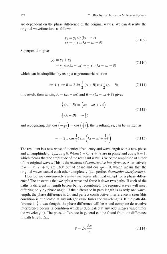
172 7 Biophysical Forces in Molecular Systems
are dependent on the phase difference of the original waves. We can describe theoriginal wavefunctions as follows:
y1 = y◦ sin(kx− ωt)y2 = y◦ sin(kx− ωt + δ) (7.109)
Superposition gives
y3 = y1 + y2
= y◦ sin(kx− ωt)+ y◦ sin(kx− ωt + δ) (7.110)
which can be simplified by using a trigonometric relation
sin A+ sin B = 2 sin1
2(A+ B) cos
1
2(A− B) (7.111)
this result, then writing A = (kx− ωt) and B = (kx− ωt + δ) gives
12 (A+ B) =
(kx− ωt + 1
2δ)
12 (A− B) = − 1
2δ
(7.112)
and recognizing that cos(− 1
2δ)= cos
(12δ)
, the resultant, y3, can be written as
y3 = 2y◦ cos1
2δ sin
(kx− ωt + 1
2δ
)(7.113)
The resultant is a new wave of identical frequency and wavelength with a new phaseand an amplitude of 2yocos 1
2 δ. When δ = 0, y1 + y2 are in phase and cos 12 δ = 1,
which means that the amplitude of the resultant wave is twice the amplitude of eitherof the original waves. This is the extreme of constructive interference. Alternativelyif δ = π , y1 + y2 are 180◦ out of phase and cos 1
2δ = 0, which means that theoriginal waves cancel each other completely (i.e., perfect destructive interference).
How do we conveniently create two waves identical except for a phase differ-ence? The answer is that we split a wave and force it down two paths. If each of thepaths is different in length before being recombined, the rejoined waves will meetdiffering only by phase angle. If the difference in path length is exactly one wave-length, the phase difference is 2π and perfect constructive interference is seen (thiscondition is duplicated at any integer value times the wavelength). If the path dif-ference is 1
2 a wavelength, the phase difference will be π and complete destructiveinterference occurs (a condition which is duplicated at any odd integer value timesthe wavelength). The phase difference in general can be found from the differencein path length, x:
δ = 2πx
λ(7.114)

7.6 Harmonic Waves Are the Result of a Sinusoidal Oscillation 173
Vector addition of harmonic waves is a very convenient method for combining morethan two waves and for considering waves of differing amplitudes. The vector addi-tion methods are reviewed in Appendix A and are easily applied once a geometricinterpretation of the wavefunction is considered. Wavefunctions are generally writ-ten either in real rectangular coordinate planes or in polar coordinate notation inwhich the amplitude of the wave is written in relation to one axis and the phaseangle is described in relation to the other. These notations can often become cum-bersome. Alternatively, it is often more convenient to write the amplitude of thewavefunction in a real plane and the phase angle in the imaginary plane. The latteris one of mathematical and notational convenience, and having phase angles in theimaginary plane has no physical meaning.Example:Find the resultant of two waves
y1 = 3 sin(kx− ωt)y2 = 6 sin(kx+ ωt + 70�)
Solution:See Fig. 7.15. Our task is to combine these waves at a particular point x and time t.The notation can be simplified by writing θ for kx – ωt. We can write
y1 = 6 sin θy2 = 3 sin (θ + 70◦)
and
y3 = y1 + y2
= 6 sin θ + 3 sin(θ + 90◦
)
= 6.708 sin θ + 26.5◦
Fig. 7.15 Vector analysis oftwo waves to give a resultantwave

174 7 Biophysical Forces in Molecular Systems
The angle θ is the constant frequency of the wave. It sweeps y1, y2, and y3 throughspace together, and the relative positions of the wave vectors are not affected.
7.7 Energy and Intensity of Waves
Waves transport energy and momentum. The transport of energy in a wave isdescribed by the wave intensity, I, which is defined as the average rate of trans-mitted energy per unit area normal to the direction of propagation. I is the averageincident energy per unit time per unit area:
I = (E/T)average
A= Pave
A(7.115)
where A is the cross-sectional area.The intensity can be written in terms of power, P, since power is energy per unit
time. How do we find E? It will be remembered that the energy in the wave isbeing supplied by an external force that is causing the wave motion. Consider thisenergy source to be inducing a harmonic wave motion in a string at the left end. Ifwe look down the string and observe a point in front of us before the wave reachesthat point, it is obvious that the string to our left contains energy but the string toour right does not yet contain this energy. As the wave sweeps past us at a velocity,v, in a certain time, t, it travels a distance equal to vt. There has now been anincrease in energy carried in the wave,E, which is equal to the average energy perunit volume of the string, η, multiplied times the unit volume of the string whichnow contains energy, namely
E = ηAvt (7.116)
The rate of energy increase, E/t, is the power. Combining Eqs. (7.115) and(7.116), the average incident power can be stated as
Pave = E
t= ηAv (7.117)
The intensity of the wave at a point is the incident power divided by the area of thestring (or propagating medium):
I = Pave
A= ηv (7.118)
Equation (7.118) is a general result applicable to all waves.What is the average energy density, η? We seek a general answer that is applica-
ble to all harmonic waves. For a harmonic wave on a string with angular frequencyω and amplitude yo, each mass element on the string moves with the energy of amass oscillating on a spring (see earlier discussion):

7.7 Energy and Intensity of Waves 175
E = 1
2(m) ω2y2◦ (7.119)
The mass of the segment can be written in terms of the mass density times volumeof the segment, ρV:
E = 1
2(ρV) ω2y2◦ (7.120)
and substituting
η = E
V= 1
2ρω2y2◦ (7.121)
so
I = ηv = 1
2ρω2y2◦v (7.122)
This general result states that the intensity of a wave is proportional to the squareof its amplitude and the square of its frequency. A direct application of Eq. (7.122)is in considering the intensity of sound, which can be a significant issue in bio-logical systems whether in using ultrasound to enhance transdermal diffusion ofpharmaceuticals or in considerations of noise pollution.
7.7.1 Sound and Human Ear
The human ear is able to respond to a large range of sound intensities from approx-imately 10−12 W/m2 to about 1 W/m2. The lower end corresponds to the thresholdof hearing while sound with an intensity of 1 W/m2 causes pain. The ear and thebrain respond to sound intensity by the sensation of loudness. Loudness varies ina logarithmic relationship to the sound intensity. Hence given the large magnitudeof the range of hearing as well as the psychological interpretation of intensity asloudness, a logarithmic scale, the decibel scale, is used to describe the intensity of asound wave. Intensity is measured in decibels, dB, which correspond to the intensityβ in the following way:
β = 10 logI
I◦(7.123)
I is the intensity which is described in dB and it is related to the threshold of hearing(Io) which is taken to be 10−12 W/m2. Using the decibel scale, the threshold forhearing is 0 dB and the threshold for pain is 120 dB. Sound intensities for a varietyof environmental sounds are often surprising when compared on the decibel scale(see Table 7.6).

176 7 Biophysical Forces in Molecular Systems
Table 7.6 Intensity ofcommon sounds Sound dB
Normal breathing 10Soft whisper at 5 m 30Quiet office 50Busy traffic on street 70Heavy truck at 15 m 90Pneumatic jack hammer 130Hearing threshold 0Rustling of leaves 20Quiet library room 40Normal voice conversation 60Factory/busy office 80Subway train 100Jet takeoff at runway 150
7.8 Standing Waves
If waves are confined within a specific space, the waves will propagate in one direc-tion and then be reflected back onto themselves. If the wavelength and constrainedspace are correctly chosen, the reflected waves and the propagating waves will con-structively interfere and give a special pattern of interference called standing waves.It is standing waves that make the sounds of a pipe organ, violin, or flute. Whena propagating wave meets its reflection the resulting interference leads to an everincreasing amplitude of the standing wave. This continues until the imperfections inthe system cause a damping of the progressive increase at a maximum amplitude.At this maximum, a state of resonance, between the exciting agent (such as a tuningfork) and the system in which the standing wave is formed (the string or pipe), issaid to have occurred. Resonance occurs when a wave propagated in a string trav-els the length of the string, is inverted and reflected and strikes the propagating end(in this case attached to a tuning fork), and is again reflected. The twice reflectedwave is inverted again and so is upright when compared to the new wave now beingpropagated by the tuning fork. The newly propagated wave and the doubly reflectedwave are of the same phase and differ only in that the first wave has already traveledtwice a distance that is twice the length of the string or 2L. The resonance conditionis thus achieved whenever twice the distance traveled is equal to the wavelength orany integer multiple of the wavelength:
2L = nλ (7.124)
It is valuable at times to consider the lowest possible frequency that can lead to aresonance condition; this frequency, f1, is called the fundamental frequency. Fromλ = v
f we can write for any frequency that will cause resonance:
f = nv
2L= nf1 (7.125)

7.8 Standing Waves 177
where f1 can be found if the velocity of the wave is known. Using the earlier resultfrom Eq. (7.96) we can write
f1 = v
2L= 1
2L
√T
μ(7.126)
The integer multiples of the fundamental frequency (given by (7.125)) are called thenatural frequencies.
The physical consequence of the resonance condition is that maximum energycan be absorbed from the active element such as the tuning fork. If the frequency ofthe tuning fork does not equal one of the natural frequencies of the string, then thewave generated by the tuning fork initially will generally remain at the amplitude ofthe fork. The reason is that over a period of time, the interference of the reflected andnewly propagated waves will add to zero and on average no energy will be absorbedby the string. You can convince yourself of the truth of this statement by graphingthis problem and roughly calculating the resultant waves.
If a string is fixed at both ends, there is not just one natural frequency but a seriesof natural frequencies which are integral multiples of the fundamental frequency.This sequence is called a harmonic series. In a state of resonance, the driving ele-ment transfers energy at a natural frequency to the string such that the waves addconstructively up to a maximum, which is ultimately limited by the damping forcespresent in the system. A wave is produced on the string that appears to stand stilland is called a standing wave. The standing wave shapes for a portion of a harmonicseries are shown in Fig. 7.16. In a standing wave system, the energy of the wave isconstant. The energy varies between a maximum potential energy when the wavecauses the string to be maximally displaced, and a maximum kinetic energy whenthe string is at the original coordinate but each segment of the string is moving atmaximum speed.
Fig. 7.16 This harmonic series shows the nodes and antinodes of the standing waves generated asmultiples of the fundamental frequency where n=1

178 7 Biophysical Forces in Molecular Systems
The mathematical form of standing waves can be found by simply finding theresultant wave derived from a wave propagated from the left, yL, and one propagatedfrom the right, yR. For simplicity we will let the amplitudes be equal and we canwrite
yR = y◦ sin (kx− ωt)yL = y◦ sin (kx+ ωt)
(7.127)
The sum of the waves is
y (x, t) = yR + yL = y◦ sin (kx− ωt)+ y◦ sin (kx+ ωt)
= 2y◦ cos (ωt)+ sin (kx)(7.128)
Equation (7.128) is the function for a standing wave. We can show this equation togive the resonance condition if we fix the string at x = 0 and x = L thus forcingy at these points to be zero for all times t. We will use a similar treatment whenwe determine the probability wave for a particle captured in a box. The boundaryconditions can then be written out:
y (x = 0, t) = 0y (x = L, t) = 0
(7.129)
Since at x= 0, sin kx= 0, the first condition is automatically met. However, there areonly a selected set of values of the wave number, k, for which the second boundarycondition, sin kL = 0, will be satisfied. Since the sin of a number is only zero at sin0 or at the sin of an integer multiple of π radians, the values of k which will satisfythe second condition are given by
kL = nπ (7.130)
Writing this in terms of wavelength where k = 2π
λ,
2π
λL = nπ (7.131)
gives the same result as the resonance condition equation (7.124):
2L = nλ (7.132)
Since the standing wavefunctions are sine waves that must fit into the boundaryconditions when n > 1, there will be other points that are at rest in addition to thetwo endpoints. These points are called nodes, and there are generally n− 1 nodes inaddition to the boundary points at rest for the nth harmonic. The points of maximaldisplacement are called antinodes and there are n antinodes for the nth harmonic.

7.9 Superposition and Interference – Waves of Different Frequencies 179
7.9 Superposition and Interference – Waves of DifferentFrequencies
We have thus far considered only the cases of superposition of waves of equal fre-quency. Waves of differing frequency will also generate resultant waves, but theresultant will often result in a complex waveform. The detailed analysis of complexwaveforms uses the mathematical techniques of Fourier analysis which are beyondthe scope of this volume. Here we will be content with a qualitative review of thesubject.
The treatment of the superposition of different frequencies is similar to the anal-ysis already undertaken. Consider the following case which we will express bothgraphically and algebraically. Two waves of equal amplitude and both moving leftto right possess different frequencies. We will consider the case of frequencies closeto one another. Initially, (i.e. when x= 0 and t= 0) both waves are in phase. Initiallythe waves will add to one another, constructively giving rise to a large resultantamplitude, but since they are out of phase, at some distance x1, their phase dif-ference will be 180◦, and there they will interfere destructively with a resultantamplitude of zero. At an equal distance x beyond x1, at x2, the waves will againbe in phase with maximal constructive interference. The greater the difference inwavelength between the two waves, the shorter will be the distance x. Algebraicallywe can write
y1 = y◦ cos (k1x− ω1t)y2 = y◦ cos (k2x− ω2t)
(7.133)
Using the cosine identity, cos A + cos B = 2 cos 12 (A− B) cos 1
2 (A+ B) theresultant wave, y(x, t) can be written as
y (x, t) = y2 + y1
= y◦ cos (k2x+ ω2t)+ y◦ cos (k1x− ω1t)
= 2y◦ cos
[1
2(k2 − k1) x− 1
2(ω2 − ω1) t
]
cos
[1
2(k2 + k1) x− 1
2(ω2 + ω1) t
]
(7.134)
Now we substitute some new notation to clean up the equation, using k and ωfor the difference in wave number and frequency and k and ω for their averages,respectively.
k = (k2 − k1) ω = (ω2 − ω1)
k = 1
2(k2 + k1) ω = 1
2(ω2 + ω1)
which allows writing

180 7 Biophysical Forces in Molecular Systems
y (x, t) = 2y◦ cos
[1
2kx− 1
2ωt
]cos
[kx− ωt
](7.135)
Now writing
y(x, t) = 2yo cos [1
2kx−1
2ωt] cos [k̂ x - ω]t (6.57)
This resultant wave has a frequency about the same as the original waves but
modulated by a factor, cos[
12kx− 1
2ωt].
Fig. 7.17 Waves of different frequency interfere in a complex way and are characterized by aphase and group velocity. Here, a Gaussian distribution of waves is combined to give the resultantwave packets. The top figure shows the wave packet at t = 0 and the lower figure shows the samewave packet at a timet later. Notice that the wave packet has moved along the x-axis in a fashionreminiscent of a particle. However, this illustration also shows some moderate dispersion of thewave packet, and the different phase and group velocity are causing the wave packet to changeshape with time

7.10 Complex Waveforms 181
The velocity of the resultant wave is
vp = ωk
(7.136)
and is called the phase velocity. The phase velocity is nearly the same as the initialwaves. The envelope of modulation outlined in Fig. 7.17 travels as a wave itself witha wave number equal to 1
2k and angular frequency of 12ω. The envelope can be
shown to have the form of a wavefunction by considering the modulation factor:
cos[1
2kx− 1
2ωt] = cos
1
2k
(x− ω
kt
)(7.137)
and defining the group velocity, vg = ωk
. Equation (7.137) can be written as
cos1
2k
(x− vgt
)(7.138)
This equation has the mathematical character of a and hence the group movesthrough space as if it were a wave itself. The group velocity and phase velocityare equal when the medium through which the wave is propagated is dispersionless,i.e., the phase velocity does not depend on the frequency of the wave. Light waves ina vacuum, sound in the air, and waves in a perfectly flexible string will not disperse.A medium in which the phase velocity depends on frequency is called a disper-sive medium, and light traveling in glass or water waves are examples. As we willsee below, this group as represented by the enveloped waves forms a distinct wavepacket with important applications in information theory, cybernetics, and quantummechanics (see Fig. 7.17).
7.10 Complex Waveforms
Complex waves are in general well treated as mixtures of harmonic waves of varyingfrequencies. Fourier’s theorem states that any periodic function can be described toan arbitrary degree of accuracy in terms of the sum of sine and cosine functions:
y(t) =∑
n
An sinωnt + Bn cosωnt (7.139)
The lowest angular frequency in the analysis will correspond to the period of thefunction under study, ω1 = 2π
T , where T is the period. All the other frequencieswill be integral multiples of this fundamental frequency. The values of An and Bn
represent the relative intensity of each of the harmonics found in the waveform andare found by Fourier analysis. The value of A2
n + B2n is proportional to the energy
of the nth harmonic of the function. The intensity of each harmonic present canbe plotted against frequency of each harmonic wave present to provide a spectral

182 7 Biophysical Forces in Molecular Systems
Fig. 7.18 An example of a Fourier analysis. A square wave is a converging geometric sum ofthe amplitudes of the odd harmonics of the fundamental frequency. (a) The left panels show theharmonic waves that create the square wave of a specific duration. The right panel shows the super-position of those waves. Note how increasing the number of harmonics summed together improvesthe Fourier representation. (b) This figure shows a power spectrum that relates the frequencies andintensities of each of those frequencies contributing to the square wave
analysis of the constituent waves in a complex function. Plots of this type are calleda power spectrum. An example of the harmonic analysis and power spectrum of asquare wave pulse is shown in Fig. 7.18.
7.11 Wave Packets
Let us now revisit the wave impulses with which we started our review. In thelast section we were using harmonic analysis to examine complex waveforms thatwere none-the-less periodic in time. Non-periodic functions (i.e., pulses) can alsobe described in terms of sine and cosine functions, but to do so requires a contin-uous distribution of frequencies rather than the discrete summation of the Fouriertheorem. Mathematically we must integrate over frequency and we will find that theconstants An and Bn become functions of frequency, A(ω) and B(ω). These constantsare often close to zero over most of the frequency range but will have non-zero valueover a specific rangeω. Pulses are quite distinct from harmonic waves in that theyclearly begin and end while harmonic waves continue repeating over and over. It isthe starting and stopping of a pulse-like signal that allows information to be sentby a wave. The relationship between distribution of the harmonic frequencies thatmake up a pulse and the duration of the pulse is important. If the duration of a pulse

7.11 Wave Packets 183
is very short, then the range of frequenciesω must be very large. The relationshipbetween frequency and time can be written as follows:
tω ≈ 1 and ω ≈ 1
t(7.140)
A wave pulse of duration t occupies a narrow band of space determined by theproduct of the time and the velocity of the wave,
x = vt (7.141)
The harmonic waves in the interval ω that comprise the pulse each have a wavenumber: k,
k = ωv
(7.142)
and thus in ω, there exist a range of wave numbers:
ω = kv (7.143)
thus we can write
kvt ≈ 1 or kx ≈ 1 (7.144)
The relationships in Eqs. (7.139) and (7.144) are important in communications the-ory and quantum mechanics, both topics of importance in understanding biologicalsystems at a molecular chemical and molecular physiological level. These rela-tionships are very important both practically and philosophically since they relatequantities that are called complementary. The relationship between energy and timeis complementary as are the observables position and momentum. The former isseen in Eq. (7.140) where ω is proportional to the energy of the packet and the lat-ter in Eq. (7.144) where the wave number is proportional to the momentum of thepacket. The concept of complementary observables is fundamental in understandingthe constraints on what is knowable in a physical system: Complete knowledge ofone aspect of the system makes any knowledge of the complementary observableimpossible.
In communications theory, information cannot be carried by an unvarying contin-uous harmonic wave. Maximal information is encoded by short pulses. The shorterthe pulse, the wider the bandwidth of the transmitting system and, hence the largerthe amount of information that can be transmitted in a fixed time. Maximizing infor-mation transfer requires the shortest possible pulse, but this means that the shortpulse contains a very large number of harmonics. A system with the capacity tohandle this wide range of frequencies without dispersion or distortion must be used.This is a primary concern in engineering communication systems both man-madeand biological.

184 7 Biophysical Forces in Molecular Systems
In quantum mechanics the impossibility of knowing values for a pair of comple-mentary observables such as position and momentum is the core of the Heisenbergindeterminacy principle. The location in space of a particle can be described in termsof a wave packet whose width is interpreted as the uncertainty in knowing the posi-tion of the particle. A very sharply defined and narrow wave packet, which leadsto a high degree of certainty in the position of the particle, must at the same timepossess a large number of associated wave numbers which are representative of themomentum of the particle. The narrower the wave packet, the more certain we areof the position. However, this condition also results in a greater number of possiblewave numbers, which represent the momentum values the particle may take, and sowe are less certain of the particle’s momentum.
7.12 Dispersion
The envelope of two waves of unequal frequency discussed above is a simplifiedcase of more complex waveforms. We will now examine qualitatively the importantand interesting effects of wave motion in a medium that is dispersive. A waveformthat travels in a dispersionless medium has a phase velocity and group velocity thatare equal. The equations written as (7.136) and (7.138) were derived for two waves,and the case can be generalized to include complex waves and wave packets. Ina wave packet, a large number of harmonic waves are superimposed over a limitedrange of wavenumbers, k, and angular frequencies, ω. Within the interval of interest,k and ω are functions dependent on one another, and we can write that ω is a functionof k. In order to write an equation that is more general than the case of just two waveswe will evaluate the function in the midpoint of the range of k or ω:
vg = ωk≈ dw
dk(7.145)
This is the generalized equation for the group velocity. What is the relationshipbetween each constitutive harmonic wave and the overall wave packet? Since eachharmonic has its own wave number and angular frequency and travels at a phasevelocity, we can write
vp = ωk= fλ (7.146)
Now we use this relationship to find the relationship between the group velocity andthe phase velocity of each constitutive harmonic:
vg = dw
dk= d
dk
(kvp
) ≈ vp + kdvp
dk(7.147)
A wave packet will change shape if the individual harmonic waves travel at speedsdifferent from the speed of the overall packet. When these shape changes occur it is

7.13 The Wave Equation 185
because the velocity of the wave is dependent in some fashion on the wave numberor its related quantities, the wavelength, or frequency. Light waves traveling througha vacuum do not disperse because there is no interaction along the way; but a lightwave in any transparent medium does interact in a frequency-dependent mannerand will be found to be dispersed by the transparent medium. A dispersion equationcan be written that links the wavenumber of a light wave to its speed in transparentmedia, and this dispersion relationship defines the refractive index of the medium.The dispersion relationship can be understood in terms of the interaction of the wavewith the elements of the medium.
7.13 The Wave Equation
The wave equation recurs throughout our studies of biophysics and some degreeof familiarity with it is important. We will discuss it here as a one-dimensionalproblem.
The wave equation is a differential equation that results directly from Newton’ssecond law; it relates the second derivative of a wavefunction with respect to x tothe second derivative with respect to time. Note that because there are two variablesthe wave equation will be the result of a partial differential equation. The generalwavefunction y(x,t) is a solution of this equation. For waves on a string or in a fluidthe wave equation can be derived from the second law with the restriction that thewave is of small enough amplitude so that the small angle approximation can bemade. Therefore the equations remain linear. For electromagnetic waves, the waveequation can be shown to derive directly from the laws of electricity without thesmall amplitude approximation.
We will show the wave equation as a result of the harmonic wavefunction.We start with the harmonic wavefunction given in Eq. (7.97):
y(x, t) = y◦ sin k(x− vt) (7.97a)
We multiply through by k and take the derivative with respect to x while holding tconstant:
∂y
∂x= ky◦ cos (kx− kvt) (7.148)
and differentiating again
∂2y
∂x2= −k2y◦ sin (kx− kvt) (7.149)
Now look at this result carefully! We have differentiated a function twice and got-ten the same function back times a constant. This is an important property of the

186 7 Biophysical Forces in Molecular Systems
class of equations we saw in the previous chapter, eigenfunctions. We can now writeEq. (7.149) in terms of the original function:
∂2y
∂x2= −k2y (x, t) (7.150)
Now we differentiate the other partial derivative, y(x,t) with respect to t with x heldconstant:
∂y
∂t= −kvy◦ cos (kx− kvt) (7.151)
and once again for the second derivative
∂2y
∂t2=−k2v2y◦ sin (kx− kvt)
=−k2v2y (x, t)(7.152)
Another eigenfunction! These can be combined to form the wave equation:
∂2y
∂x2= 1
v2
∂2y
∂t2(7.153)
For a wave on a string y represents the displacement of the string, for a sound wavey is the pressure or density change, and for an electromagnetic wave y is the electricor magnetic field magnitude. Equation (7.82) applies to any wave propagating inone dimension without dispersion that can be shown by evaluating the more generalfunctions given in Eqs. (7.141) and (7.143).
The wave equation is linear (i.e., it has no roots or derivatives that are to anypower except the first power). The principle of superposition naturally derives fromthis linearity since linear equations have the property that if y1 (x, t) and y2 (x, t) aresolutions of the equation, the linear combination
y (x, t) = C1y1 (x, t)+ C2y2 (x, t) (7.154)
is also a solution. Thus any two waves satisfying the wave equation can be simplyadded and their resultant will also satisfy the equation.
7.14 Waves in Two and Three Dimensions
Now we generalize our discussions of one-dimensional waves to two and threedimensions which are the wave systems with which we more commonly deal.Consider a point source generating a harmonic wave. Figure 7.19 shows how a cir-cular (two-dimensional) or a spherical (three-dimensional) wave is generated witha point source as the origin. In the case of a spherical wave, the first sphere atdistance r from the origin has an area of 4πr2. The energy is evenly distributed

7.14 Waves in Two and Three Dimensions 187
Fig. 7.19 The shape of apropagating wave in (a) one,(b) two, andg (c) threedimensions
over this area. At each subsequent sphere nr from the origin, the same energy isdistributed over an area of 4πnr2 so the intensity decreases as 1
r2 . This relationshipholds even when energy is not equally radiated as can be shown if a cone of energy isconsidered.
Since the intensity of a wave is proportional to the square of its amplitude, theamplitude of a spherical wave must vary as 1
r . The wavefunction, ψ , of a sphericalwave is written as
ψ(r, t) = A◦r
sin(kr − ωt + δ) (7.155)
where the constant Ao is independent of r, and δ, as before, is a phase constant.The phase of this wave is constant on a spherical surface at any given time. Sucha surface of constant phase is called a wavefront. Wavefronts are usually drawn atthe maximum amplitude of the wave, and the radial distance between successivemaxima is the wavelength. The phase velocity v is calculated as v = fλ. A veryconvenient rendering of spherical waves is the ray tracing (Fig. 7.20a), and we can

188 7 Biophysical Forces in Molecular Systems
Fig. 7.20 Representation of (a) the ray tracing abstraction of a spherical wave. (b) Ripple tankproduction of a plane wave. (c) At a distance from the point of propagation, a spherical wave canbe treated as a plane wave

Problem Sets 189
see both the advantages and limitations of such an abstraction in Appendix G. Whenthe wavefronts are far away from the point source, the curvature of the wavefront isso small that the ray is essentially perpendicular to the wavefront, and the sphericalwave appears to be a plane wave (Fig. 7.20c). A two-dimensional representation ofa plane wave can be generated in a ripple tank by the oscillation of a flat object upand down (Fig. 7.20b). When a spherical wave has reached the point at which itcan be regarded as a plane wave, the wavefronts move perpendicular to the x axisin a series of yz planes. At this point the phase depends only on x and t and thewavefunction has the same form as a one-dimensional wave:
ψ(x, t) = A◦ sin(kx− ωt + δ) (7.156)
Plane waves traveling in a featureless and unobstructed medium will act inidentical fashion to the one-dimensional waves that we have examined. If theystrike an infinitely long boundary in the yz plane, the wave can be treated asbeing reflected like a one-dimensional wave. However, if a plane wave runs intoapertures or obstructions, the plane symmetry is destroyed and it will act onceagain like a three-dimensional wave. The consequences of these distortions lead toreflection, refraction and diffraction and are phenomena with immensely importantimplications both theoretically and practically.
Further Reading
See the listed readings in Chapter 6.
Problem Sets
1. (a) Calculate the proportionality coefficient of the ideal gas law, R, the gas con-stant from the ideal gas law using STP. (b) Use the conversion factors listed inthe appendix to express R in units of J/K/mol.
2. Use the van der Waals equation to determine the molecular size of a gas atom ofhelium, neon, and water vapor.
3. Ion channels allow ion flow through the lipid membrane of a cell. Many channelsare selective allowing only certain ions through. Some channels have a selectivityfilter that prevents anions even of the appropriate charge from penetrating into achannel reserved for cationic species. The selectivity filter can be modeled as aring of charge around the mouth of the channel. Calculate the force on a pointcharge as it moves on the axis of a uniformly distributed ring of charge. Calculatefor an anion of charge –1, −2 and a cation of charge +1, +2.
4. Calculate the force due to a spherically symmetrical charge distribution, i.e., acell interacting with an ion or proton.
5. Calculate the electric field at distance R from an infinite sheet of charge withuniform surface charge.

190 7 Biophysical Forces in Molecular Systems
6. A popular act of violence in the movies is the electrocution of a character whilethey are taking a bath by having an electrical appliance such as a hair dryer orlamp thrown into the tub of water.
a) Draw a potential map showing the isoelectric lines for this situation.b) Is it fact or fantasy that the act of violence is successful?