antenna and microwave engineering - NEDUET - NED ...

LABORATORY WORK BOOK For Academic Session _______

Semester _____

ANTENNA AND MICROWAVE ENGINEERING

(TC-313)

For

TE (TC)

Name:

Roll Number:

Batch:

Department:

Year/Semester:

Department of Electronic Engineering NED University of Engineering & Technology, Karachi

LABORATORY WORK BOOK

For The Course

TC-313 ANTENNA AND MICROWAVE ENGINEERING

Prepared By:

Farzeen Iqbal (Lecturer)

Nida Nasir (Assistant Professor)

Reviewed By

Dr. Irfan Ahmed (Associate Professor)

Approved By:

Board of Studies of Department of Electronic Engineering

INTRODUCTION Antenna & Microwave Engineering Practical Workbook covers a variety of experiments that are designed to aid students in their profession and theory. The practical are very beneficial to students and will help them in having a core knowledge and understanding of the subject. The practical covered in this manual give more than a basic introduction to students. They cover a variety of topics which include antennas, transmission lines and microwave waveguides. A practical exposure to such equipment is necessary as it builds on the theory taught to students. The practical are based on modern trainers that incorporate a variety of functions to demonstrate to students the principles of Antenna & Microwave Engineering techniques. The students will develop a profound interest in this course which will facilitate them whether it is in future professional work or higher studies.

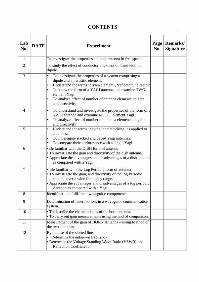
CONTENTS

Lab No. DATE Experiment Page

No. Remarks/ Signature

1 To investigate the properties a dipole antenna in free space

2 To study the effect of conductor thickness on bandwidth of dipole

3 • To investigate the properties of a system comprising a dipole and a parasitic element.

• Understand the terms ‘driven element’, ‘reflector’, ‘director’ • To know the form of a YAGI antenna and examine TWO

element Yagi. • To analyze effect of number of antenna elements on gain

and directivity

4 • To understand and investigate the properties of the form of a YAGI antenna and examine MULTI element Yagi.

• To analyze effect of number of antenna elements on gain and directivity

5 • Understand the terms ‘baying’ and ‘stacking’ as applied to antennas.

• To investigate stacked and bayed Yagi antennas. • To compare their performance with a single Yagi.

6 • Be familiar with the DISH form of antenna. • To investigate the gain and directivity of the dish antenna. • Appreciate the advantages and disadvantages of a dish antenna

as compared with a Yagi

7 • Be familiar with the Log Periodic form of antenna • To investigate the gain, and directivity of the log Periodic

antenna over a wide frequency range. • Appreciate the advantages and disadvantages of a log periodic

Antenna as compared with a Yagi.

8 Identification of different waveguide components.

9 Determination of Insertion loss in a waveguide communication system.

10 • To describe the characteristics of the horn antenna. • To carry out gain measurements using method of comparison.

11 Measurement of the gain of HORN Antenna – using Method of the two antennas

12 By the use of the slotted line, • Determine the unknown frequency • Determine the Voltage Standing Wave Ratio (VSWR) and

Reflection Coefficient.

13 By use of slotted waveguide • Observe how the load impedance affects the VSWR. • Determine when a waveguide is properly terminated

14 To measure unknown load impedance attached to a waveguide using the smith chart.

15 Familiarization with VNA: Vector Network Analyzer • Front panel tour Setup keys Display Formats and Diagram Types:

a) Cartesian Diagram b) Polar Diagram c) Smith Chart

16 Measurement of S parameters of available filter

TC-313 Antenna and Microwave Engineering NED University of Engineering and Technology- Department of Electronic Engineering

1

LAB SESSION 01 OBJECT:- To investigate the properties a dipole antenna in free space EQUIPMENT:- Antenna Lab hardware Discovery Software Dipole elements Yagi boom THEORY: Antenna: An antenna is a transducer designed to transmit or receive radio waves which are a class of electromagnetic waves. In other words, antennas convert radio frequency electrical currents into electromagnetic waves and vice versa. Antennas are used in systems such as radio and television broadcasting, point-to-point radio communication, wireless LAN, radar, and space exploration. Antennas usually work in air or outer space, but can also be operated under water or even through soil and rocks at certain frequencies for short distances. Physically, an antenna is an arrangement of conductors that generate a radiating electromagnetic field in response to an applied alternating voltage and the associated alternating electric current, or can be placed in an electromagnetic field so that the field will induce an alternating current in the antenna and a voltage between its terminals. Simple Dipole Antenna: just about the simplest form of antenna is called the dipole. This is a conductor that is divided in the middle and is connected at this point to a feeder (or feed line). This feeder then connects the antenna to the receiver, or transmitter. Feeders come is many forms. Probably, the most commonly used is coaxial cable. This is the type of feeder used in this trainer.

Generally, the dipole is considered to be Omni-directional in the plane perpendicular to the axis of the antenna, but it has deep nulls in the directions of the axis.


2

PRE LAB TASK:

1. Discuss Dipole Antenna Characteristics: • Frequency Vs. Length • Radiation Pattern and Gain. • Feeder Line 2. Write Common applications of Dipole Antenna.

PROCEDURE: 1. Identify one of the antenna Boom Assemblies and mount it on top of the Generator Tower. 2. Ensure that all of the elements are removed, except for the dipole. 3. Examine the dipole element; you will see that the ends are extendible. Adjust the dipole

length so that it is 5cm either side of the centre. 4. Ensure that the Motor Enable switch is off and then switch on the trainer. 5. Launch signal strength vs. angle 2D polar graph and immediately switch on the motor

enable. 6. Ensure that the Receiver and Generator antennas are aligned with each other and that the

spacing between them is about one meter. 7. Acquire a new plot at 1500MHz. 8. Observe the polar plot.


3

OBSERVATIONS: 1. Does the dipole antenna have the same response in all directions in the azimuth (horizontal)

plane?

2. In which direction(s) is the response a maximum?

3. In which direction(s) is the response a minimum? RESULT:


4

LAB SESSION 02 OBJECT:- To study the effect of conductor thickness on bandwidth of dipole EQUIPMENT:- Electronica Veneta (turntable) with stand Field meter SFM 1 EV Microwave generator 75ohm coaxial cable Basic dipole antenna short thick conductors (8mm) Basic dipole antenna Short Thin dipole (3mm) THEORY:- Dipole: It consists of two poles that are oppositely charged. Dipole antenna: The simple dipole is one of the basic antennas. It is an antenna with a center-fed driven element for transmitting or receiving radio frequency energy. This is the directed antenna i.e. radiations take place only forward or backward. Its characteristic impedance is 73. Half wave dipole: Half wave dipole is an antenna formed by two conductors whose total length is half the wave length. In general radio engineering, the term dipole usually means a half-wave dipole (center-fed) Thin and thick dipole: Theoretically the dipole length must be half wave; this is true if the wavelength/conductor’s diameter ratio is infinite. Usually there is a shortening coefficient K (ranging from 0.9-0.99)according to which the half wavelength in free space must be multiplied by K in order to have the half wave dipole length, once the diameter of the conductor to be used is known.(refer fig) Bandwidth: The range of frequencies in which maximum reception is achieved. Effect of thickness: By increasing the conductor diameter in respect to the wavelength, the dipole characteristic impedance will increase too in respect to the value of 73. On the other hand outside the center frequency range, the antenna reactance varies more slowly in a thick than in a thick antenna. This means, with the same shifting in respect to the center frequency, the impedance of an antenna with larger diameter is more constant and consequently the SWR assumes lower values. Practically the bandwidth is wider.


5

PROCEDURE: 1. Construct a dipole with arms of 3mm diameter (short) and mount on the central support of the

turntable. 2. Set the antenna and instruments as shown above in figure. 3. Set the generator to a determinate output level and to the center frequency of the antenna under

test. 701.5 MHz for measurements with short (thick or thin dipole). 4. Adjust the dipole length and sensitivity of the meter to obtain the maximum reading (10th LED

glowing). 5. Now decrease the frequency up to the value such that the 10th LED keeps on glowing. Note the

value as f2. 6. Now increase the frequency up to the value such that the 10th LED keeps on glowing. Note the

value as f1. 7. Calculate the wavelength for the resonance frequency of around 700 MHz for short dipole using

the formula λ=c/f. 8. The ratio used for calculating the shortening coefficient is λ/2d where d=diameter of conductor. 9. From graph obtain a shortening coefficient K Calculate the physical length of Dipole and

compare with the measured length. 10. Physical length of half wavelength dipole= [λ/2] x K. 11. Construct a dipole with arms of 8mm diameter (short). 12. Repeat the same procedure for thick dipole.


6

OBSERVATIONS & CALCULATIONS:- • Resonant frequency = MHz • λ = c/f = 300/ = cm • Measured length of short dipole thin= 220mm • Measured length of short thick dipole=195mm THIN dipole: d=

• The ratio used for calculating the shortening coefficient is (with a dia of 3mm) λ/2d = K=

• From graph we obtain a coefficient of 0.960 for the thin dipole • Physical length of half wavelength dipole= 2λ x K=

THICK dipole: d=

• The ratio used for calculating the shortening coefficient is with a diameter of 8mm λ/2d=K=

• From graph we obtain a coefficient of 0.947 for thick dipole • Calculated physical length of half wavelength dipole= 2λx K= (These values refer to a dipole in air. Actually the dipole under consideration is not totally in air because for mechanical reasons, its internal part is in a dielectric. This slightly increases the resonance frequency.) RESULT:


7

LAB SESSION 3 OBJECT:-

• To investigate the properties of a system comprising a dipole and a parasitic element. • Understand the terms ‘driven element’, ‘reflector’, ‘director’ • To know the form of a YAGI antenna and examine TWO element Yagi. • To see how gain and directivity increase as element numbers increase

EQUIPMENT:- Antenna Lab hardware Discovery Software Dipole elements Yagi boom THEORY:- Antenna: An antenna is a transducer designed to transmit or receive radio waves which are a class of electromagnetic waves. In other words, antennas convert radio frequency electrical currents into electromagnetic waves and vice versa. Antennas are used in systems such as radio and television broadcasting, point-to-point radio communication, wireless LAN, radar, and space exploration. Antennas usually work in air or outer space, but can also be operated under water or even through soil and rocks at certain frequencies for short distances. Physically, an antenna is an arrangement of conductors that generate a radiating electromagnetic field in response to an applied alternating voltage and the associated alternating electric current, or can be placed in an electromagnetic field so that the field will induce an alternating current in the antenna and a voltage between its terminals. Yagi Uda Antenna: An antenna with a driven element and one, or more, parasitic element is generally known as a “yagi”, after on of its inventors (Yagi and Uda). With the length of the second dipole (the un-driven or “Parasitic” element) shorter then the driven dipole (the driven element) the direction of maximum radiation is from the driven element towards the parasitic element. In this case, the parasitic element is called the “director”. With the length of the second dipole longer than the driven dipole the direction of maximum radiation is from the parasitic element towards the driven element. In the case, the parasitic element is called the “reflector”.


8

PRE-LAB TASKS:

1. Why do we require Arrays? Give Reasons.

2. Discuss different types of Antenna Arrays

3. How are BEAMWIDTH, DIRECTIVITY and GAIN related? PROCEDURE & OBSEVATIONS: 1. Identify one of the Yagi Boom Assemblies and mount it on top of the Generator Tower. 2. Ensure that all of the elements are removed, except for the dipole. 3. Ensure that the Motor Enable switch is off and then switch on the trainer. 4. Launch signal strength vs. angle 2D polar graph and immediately switch on the motor


spacing between them is about one meter. 6. Set the dipole length to 10cm. 7. Acquire a new plot at 1500MHz. Observe the polar plot. 8. Identify one of the other undriven dipole antenna element. 9. Move the driven dipole forward on the boom by about 2.5 cm and mount a second undriven

dipole element behind the first at a spacing of about 5 cm. 10. Set the undriven length to 10 cm. 11. Acquire a second new plot at 1500 MHz. Has the polar pattern changed by adding the second element? 12. Change the spacing to 2.5cm and acquire a third new plot at 1500 MHz What changes has the alteration in spacing made to the gain and directivity?

CHANGING THE LENGTH OF THE PARASITIC ELEMENT: 13. Launch new signal strength vs. angle 2D polar graph window. 14. Acquire a new plot at 1500 MHz. 15. Extend the length of the un-driven element to 11cm. 16. Acquire a second new plot at 1500 MHz. 17. Reduce the length of the un-driven element to 8cm.


9

18. Acquire a third new plot at 1500MHz.

What changes has the alteration in length made to the gain and directivity? RESULT:


10

LAB SESSION 04 OBJECT:-

• To investigate the properties of a system comprising a dipole and a parasitic element. • Understand the terms ‘driven element’, ‘reflector’, ‘director’ • To know the form of a YAGI antenna and examine MULTI element Yagi. • To see how gain and directivity increase as element numbers increase

EQUIPMENT:- Antenna Lab hardware Discovery Software Dipole elements Yagi boom THEORY:- Antenna: An antenna is a transducer designed to transmit or receive radio waves which are a class of electromagnetic waves. In other words, antennas convert radio frequency electrical currents into electromagnetic waves and vice versa. Antennas are used in systems such as radio and television broadcasting, point-to-point radio communication, wireless LAN, radar, and space exploration. Antennas usually work in air or outer space, but can also be operated under water or even through soil and rocks at certain frequencies for short distances. Physically, an antenna is an arrangement of conductors that generate a radiating electromagnetic field in response to an applied alternating voltage and the associated alternating electric current, or can be placed in an electromagnetic field so that the field will induce an alternating current in the antenna and a voltage between its terminals. Yagi Uda Antenna: An antenna with a driven element and one, or more, parasitic element is generally known as a “Yagi”, after on of its inventors (Yagi and Uda). With the length of the second dipole (the un-driven or “Parasitic” element) shorter than the driven dipole (the driven element) the direction of maximum radiation is from the driven element towards the parasitic element. In this case, the parasitic element is called the “director”. With the length of the second dipole longer than the driven dipole the direction of maximum radiation is from the parasitic element towards the driven element. In the case, the parasitic element is called the “reflector”.


11

PRE-LAB TASKS:

1. Why do we require Arrays? Give Reasons.

2. Discuss different types of Antenna Arrays

3. How are BEAMWIDTH, DIRECTIVITY and GAIN related? PROCEDURE & OBSEVATIONS:

1. Identify one of the Yagi Boom Assemblies and mount it on top of the Generator Tower. 2. Ensure that all of the elements are removed, except for the dipole. 3. Ensure that the Motor Enable switch is off and then switch on the trainer. 4. Launch signal strength vs. angle 2D polar graph and immediately switch on the motor


spacing between them is about one meter. 6. Set the dipole length to 10cm. 7. You have already acquired a plot at 1500MHz for TWO element Yagi in the previous lab.

Now, ADD A SECOND REFLECTOR:

8. Mount the driven dipole on the boom forward from the axis of rotation by about 2.5cm and mount a second un-driven dipole element behind the first, at a spacing of about 5cm.

9. Set the dipole length to 10cm and the un-driven dipole length to 11cm 10. Acquire a new plot at 1500MHz. 11. Observe the polar plot

Is there any significant difference between the two plots?

12. Mount a second parasitic element about 5cm from the first parasitic reflector and adjust its length to 11cm.

13. Acquire a second new plot at 1500MHz. Observe the polar plot. 14. Change the spacing between the two reflectors and acquire a third new plot at 1500MHz. Is there any significant difference between the plots, now? You will find that the addition of a second reflector has little effect on the gain and directivity of the antenna, irrespective of the spacing between the two reflectors.


12

ADDING DIRECTORS: 15. Remove the second reflector element from the boom 16. Launch new signal strength vs. angle 2D polar graph window. 17. Acquire a new plot at 1500 MHz. Observe the polar plot. 18. Mount a parasitic element about 5cm in front of the driven Element and adjust its length to 8.5cm 19. Acquire a second new plot at 1500 MHz, Observe the polar plot. Is there any significant difference between the two plots? 20. Move the director to about 2.5 cm in front of the driven element. 21. Acquire a third new plot at 1500 MHz, Observe the polar plot. How does the new plot compare with the previous two? 22. Launch signal strength vs. angle 2d polar graph window. 23. Acquire a new plot at 1500 MHz. 24. Add a second director 5 cm in front of the second. 25. Acquire a second new plot at 1500 MHz. 26. Add a third director 5 cm in front of the second. 27. Acquire a third new plot at 1500 MHz 28. Add a fourth director 5 cm in front of the third. 29. Acquire a fourth new plot at 1500 MHz. How do the gains and directivities compare? 30. Launch signal strength vs. angle 2D polar graph window. 31. Acquire a new plot at 1500 MHz. 32. Move the reflector to 2.5 cm behind the driven element. Acquire a second new plot at 1500 MHz. Does the driven element – reflector spacing has much effect on the gain or directivity of the antenna? RESULT:

- 13 -

LAB SESSION 05 OBJECT:

• Understand the terms ‘baying’ and ‘stacking’ as applied to antennas. • To investigate stacked and bayed Yagi antennas. • To compare their performance with a single Yagi.

EQUIPMENT: Antenna Lab hardware Discovery Software 6 element log periodic antenna THEORY: Yagi antennas may be used side-by-side, or one on top of another to give greater gain or directivity. This is referred to as baying, or stacking the antennas, respectively.

PRE-LAB TASK:

1. Which configuration of the two appears better than the other and why? PROCEDURE & OBSERVATIONS: Baying Two Yagis:

1. Connected up the hardware of Antenna Lab. 2. Loaded the Discovery software. 3. Loaded the NEC-Win software 4. Ensure that a Yagi Boom Assembly is mounted on the Generator Tower. 5. Building up a 6 element Yagi. The dimensions of this are:

Length(cm) Spacing Reflector 11 5cm behind driven

element

- 14 -

Driven element 10 Zero (reference) Director 1 8.5 2.5 cm in front of DE Director 2 8.5 5 cm in front of D1 Director 3 8.5 5 cm in front of D2 Director 4 8.5 5 cm in front of D3

6. Plot the polar response at 1500 MHz 7. Without disturbing the elements too much, remove the antenna from the Generator Tower

Identify the Yagi Bay base assembly (the broad grey plastic strip with tapped holes) and mount this centrally on the Generator Tower.

8. Mount the 6 element Yagi onto the Yagi Bay base assembly at three holes from the centre Assemble an identical 6 element Yagi on the other Yagi Boom Assembly and mount this on the Yagi Bay base assembly at three hole the other side of the centre, ensuring that the two Yagis are pointing in the same direction (towards the Receiver Tower).

9. Identify the 2-Way Combiner and the two 183mm cables. 10. Connect the two 183mm cables to the adjacent connectors on the Combiner and their

other ends to the two 6 element Yagis. 11. Connect the cable from the Generator Tower to the remaining connector on the Combiner 12. Acquire a new plot for the two bayed antennas onto the same graph as that for the single 6

element Yagi. 13. Reverse the driven element on one of the Yagis and acquire a third plot Does reversing the driven element make much difference to the polar pattern for the two bayed Yagis? How does the directivity of the two bayed Yagis compare with the single Yagi plot (with the driven element the correct way round)? How does the forward gain of the two bayed Yagis compare with the single Yagi plot (with the driven element the correct way round)? Now, move the two Yagis to the outer sets of holes on the Yagi Bay base assembly. Ensure that you keep the driven elements the same way round as you had before to give the correct phasing. Superimpose a plot for this assembly. How do the directivity and forward gain of the wider spaced Yagis compare with the close spaced Yagis?

Stacking Two Yagis:

- 15 -

1. Identify the Yagi Stack base assembly (the narrow grey plastic strip with tapped holes) and mount this on the side of the Generator Tower.

2. Mount the 6 element Yagi onto the Yagi Stack base assembly at one set of holes above the centre.

3. Plot the polar response at 1500 MHz. 4. Mount the other 6 element Yagi on the Yagi Stack base assembly at the uppermost set of

holes, ensuring that the two Yagis are pointing in the same direction (towards the Receiver Tower)

5. Identify the 2-Way Combiner and the two 183mm coaxial cables. 6. Connect the two 183mm cables to the adjacent connectors on the Combiner and their

other ends to the two 6 element Yagis. 7. Connect the cable from the Generator Tower to the remaining connector on the

Combiner. 8. Superimpose the polar plot for the two stacked antennas onto that for the single 6 element

Yagi. 9. Reverse the driven element on one of the Yagis and superimpose a third plot 10. Change the position of the lower Yagi to the bottom set of holes on the Yagi Stack base

assembly. Ensure that the driven elements are correctly phased and superimpose a fourth polar plot.

How does the directivity of the different configurations compare? How does the forward gain of the stacked Yagis compare with the single Yagi? How does the forward gain of the stacked Yagis change when the driven element phasing is incorrect? RESULT:

- 16 -

LAB SESSION 06

OBJECT: • Be familiar with the DISH form of antenna. • To investigate the gain and directivity of the dish antenna. • Appreciate the advantages and disadvantages of a dish antenna as compared with a Yagi.

EQUIPMENT: Antenna Lab hardware Discovery Software Parabolic Dish reflector Dipole (10cm) Yagi boom Ground plane reflector THEORY: A dish can be thought of as a passive reflector that focuses the energy from a source into one direction, much like a parabolic mirror focuses light. However, to perform as efficiently as an optical reflector, a dish needs to be in excess of ten wavelengths in diameter for the frequency being used. This is very often not the case in practice, due to physical size constraints. A horn antenna is often used to, launch or capture energy from a dish reflector. Although this is quite common, a simple dipole is often used to perform the same task. The dish set-up with Antenna Lab is one that uses a dipole at, or close to, the focus of a 60cm parabolic dish.

The dimensions for a dish are shown in figure. The focal length for a parabolic dish is given by

The gain of a dish is given by:

Where, ‘G’ is the gain, ‘a’ is the area of the dish, ‘c’ is the dish efficiency and ‘λ’ is the wavelength. Note that this is dBi, your measured gain will be dBi. For the dish with Antenna Lab at 1500 MHz the efficiency is about 0.5, f=37.5cm, D=57.4cm and d=5.5cm

- 17 -

. PRE-LAB TASKS:

1. What is Parabola? Why its geometry makes it suitable to be used as Antenna Reflector?

2. Describe different methods of feeding Parabolic Reflector. PROCEDURE & OBSERVATIONS:

1. Connect the hardware of Antenna Lab s described in the Operators Manual. 2. Load the Discovery software as described in the Operators Manual. 3. Mount the Yagi Boom Assembly on top of the Generator Tower and place the dipole at the

centre, directly above the tower 4. Set the length of the dipole to 10cm 5. Do not connect up the coaxial cable to the dipole 6. Launch new signal strength vs. angle 2D polar graph. 7. Because the dish is a physically large structure, the speed of rotation of the system must be

lowered for this Assignment. From the menu select Tools, then change, Motor Speed. Select a value of approximately 60 % and click OK.

8. Now, connect up the cable. 9. Plot the polar response of the dipole at 1500 MHz 10. Remove the Yagi Boom assembly from the tower. 11. Identify the Dish Antenna 12. Mount the Yagi Boom assembly onto the Dish and position the dipole towards the end with

the plane reflector at the end of the boom. 13. Mount this assembly onto the Generator tower 14. Ensure the length of the dipole is 10cm. 15. Set the distance from the dipole to the dish to be 38cm.

16. Set the plane reflector 5cm in front of the dipole (Further from the dish). 17. Superimpose a new plot to observe the response of the dish at 1500 MHz.

- 18 -

Does the dish antenna have gain over the dipole at 1500 MHz? Does the dish antenna have directivity at 1500 MHz?

Does the measured gain of the dish antenna agree with the theoretical gain at 1500 MHz?

18. Superimpose polar plots for frequencies of 1200 MHz, and 1300 MHz 1400 MHz on the 1500 MHz one.

Does this dish Antenna have directivity over this range of frequencies?

19. Superimpose polar plots for frequencies of 1600 MHz and 1800 MHz on the 1500 MHz one. Does the dish antenna have gain over this range of frequencies?

20. Increase the spacing to 6 cm and superimpose another new plot Does the response change significantly?

21. Reduce the distance from the dipole to the dish by 1 cm whilst maintaining the spacing of the plane reflector from the dipole of 5 cm and superimpose a second 1500 MHz polar plot.

22. Reduce the distance from the dipole to the dish by another 1cm whilst maintaining the spacing of the plain reflector from the dipole of 5cm and superimpose another 1500MHz plot.

Does the response change significantly?

23. Try for other distance and reflector spacing

- 19 -

Is the response of the dish antenna critically dependant on the spacing? RESULT:

- 20 -


• Be familiar with the Log Periodic form of antenna • To investigate the gain, and directivity of the log Periodic antenna over a wide frequency range. • Appreciate the advantages and disadvantages of a log periodic Antenna as compared with a

Yagi. EQUIPMENT: Antenna Lab hardware Discovery Software 5 element log periodic Antenna Directional coupler THEORY: The Yagi antennas that you have been investigating are inherently narrow-bandwidth antennas. The relatively small range of frequencies over which the VSWR is below 2:1 has demonstrated this. The log periodic antenna is a design that attempts to cover a much wider bandwidth. With a Yagi all of the elements are active on the operating frequency. With a log periodic antenna only a number of the elements will be active on any one frequency, the actual elements that are active changes as the frequency is changed. The role of active elements is passed from the longer to the shorter elements as the frequency increases. View of the assembly required for this assignment.

PRE-LAB TASKS:

- 21 -

Q. We say that “a log-periodic antenna (LP, also known as a log-periodic array) is a broadband, multi-element, unidirectional, narrow-beam antenna that has impedance and radiation characteristics that are regularly repetitive as a logarithmic function of the excitation frequency. The individual components are often dipoles, as in a log-periodic dipole array (LPDA). Log-periodic antennas are designed to be self-similar and are thus also fractal antenna arrays. Define each of the terms (6) (in bold letters). PROCEDURE & OBSERVATIONS:

1. Connect up the hardware of Antenna 2. Load the Discovery software 3. Mount the Yagi boom assembly on top of the generator tower and Position the dipole at the

center, directly above the tower. 4. Set the length of the dipole to 10cm 5. Plot the polar response of the dipole at 1500 MHz. 6. Remove the Yagi boom assembly from the tower 7. Identify the 5 elements log periodic Antenna with its feeder cable. 8. Mount this antenna on the Generator tower and connect the cable. 9. Superimpose the response for this antenna at 1500MHz.

Does the log periodic antenna have gain over the dipole at 1500 MHz? Does the log periodic antenna have directivity at 1500 MHz?

10. Using a new graph window, plot the polar response for 1500 MHz again 11. Superimpose polar plots for frequency of 1200 MHz, 1300MHz and 1400MHz on the

1500MHz one. Does the log periodic antenna have gain over this range of frequencies? Does the log periodic antenna have directivity at over this range of frequencies?

12. Restart and plot the response for 1500 MHz again. 13. Superimpose polar plots for frequency of 1600 MHz, 1700 MHz and 1800 MHz on the 1500

MHz one.

What happens to the gain of the log periodic antenna over this range of frequencies?

- 22 -

Does the log periodic antenna still have directivity over this range of frequencies?

14. Launch a return loss vs. frequency graph window. Identify the directional coupler and connect it. Plot the VSWR (Return loss) vs. frequency.

Is the VSWR response of the antenna greatly dependant on frequency? RESULT:

- 23 -

LAB SESSION 08 OBJECT: Identification of different waveguide components. EQUIPMENT: Wave-Guide (mod.MW-2 I mod.MW-3) WG/COAX adapter (mod.MW·1) Slotted Line (mod.MW-5) BNC-SMA detector (mod. MW-4) Coaxial Attenuator (mod.MW-23) Matched Load Termination (mod.MW-9) Short-Circuit (mod.MW-10) Variable Attenuator (mod.MW-6) THEORY: There are many components designed for operation at microwave frequencies. Some of these used in our laboratory experiments are: WG/COAX adapter (mod.MW·1): The Wave-guide to Coaxial adapter or "WG to Coax" is used to convert the electromagnetic field (E-H) present in the wave-guide into electrical signal in the coaxial cable. Obviously its function is performed in both directions, so also from electrical signal to electromagnetic field. See Figure 1. The commonly available adapters are set for the excitation of the electrical fields inside the wave-guide: this occurs introducing a conductor inside the guide (Figure 2), at a distance of λg/4 (λg is the wave-length in the guide) from the rear side, so that the reflected and the incident waves are in phase. Even the height X is about λg/4 and each component is singularly matched for the best performances. Our adaptor is Coaxial cable kind: SMA-female, VSWR: 1.25 max.

Wave-Guide (mod.MW-2 I mod.MW-3): The "wave-guide" is more properly called "WG Straight section". It is used as a transmission line and there are rigid or flexible versions of different kind, that enable the transferring of the electromagnetic field inside it. Important characteristics are low loss and VSWR. Our system uses three rigid and straight ones with the following characteristics, Figure 3.

- 24 -

Figure 3

Slotted Line (mod.MW-5) : It is a device used to detect the standing wave inside the guide (Figure 4). The Detector (mod.MW-4) must be used and is screwed on the upper part of the trailer that slides along the slot of the wave-guide. The voltage provided by the detector is proportional to the amplitude of the standing wave in the different positions along the line

Figure 4

BNC-SMA detector (mod. MW-4): Inside, the detector is characterized by the following components

• Input RF matching impedance DC Return • RF by-pass capacitor • Detector diode (with negative polarity)

The input of the detector is designed to match the signal that is to be analyzed on 50 Ohm. The DC output is commonly called Video output. See Figure 5.

Figure 5

Coaxial Attenuator (mod.MW-23): The coaxial attenuator is a passive component inserted into a metal container (Figure 6). The input and the output use the SMA coaxial connector and are matched on 50ohm. Its function is to attenuate the level of the RF signal to the input of 20dB. In particular, 20 dB corresponds to Attenuation equal to:

• 100 times in power, and • 10 times in voltage

If the attenuator is used, e.g., across the output of an amplifier stage, the total output level after the attenuator will be reduced of 20 dB, if it is expressed in dBm (measurement unit of the power referred to 1mW) as well as in dB J.l (measurement unit of the voltage referred to IJ.lV).

- 25 -

The attenuator is used when in presence of strong signals that could damage the next circuit, saturate the states of a receiver or a meter or when it is necessary for the signal level to be inside a fixed level range.

Figure 6

Matched Load Termination (mod.MW-9): The termination or fictitious load is a device absorbing the RF power without causing reflections (Figure 7). It consists of a WG straight section of wave-guide closed in short-circuit, with absorbing material (for the RF) that starts from the short-circuit and restricts to the open side. The particular shape with triangular section enables the gradual and complete absorption of the incident power to prevent reflections. Important characteristic is the low VSWR.

Figure 7

Short-Circuit (mod.MW-10): It is short-circuit termination for wave-guide. It uses the completely closed standard flange that causes the complete reflection of the whole incident RF signal. See Figure 8.

Figure 8

Variable Attenuator (mod.MW-6): It consists of a "WG straight section" where a plate is mounted in the central part and the intensity of the electrical field is maximum. The depth of insertion of the plate is adjustable and the introduced attenuation varies consequently. See Figure 9. The attenuation level can be adjusted from 0.5dB to roughly 30dB. VSWR is around 1.20.

- 26 -

Figure 9

OBSERVATION & RESULTS:

- 27 -

LAB SESSION 09 OBJECT: Determination of Insertion loss in a waveguide communication system. EQUIPMENT: 1 Transmitter Module MW-TX. 1 Up Converter unit module MW-UC. 1 VSWR/LEVEL meter unit module MW-MT. 2 Waveguide modules MW-3. 2 WG/Coax Adapter Module MW-1. 1 Fixed attenuator module MW-8. 1 Fixed attenuator module MW-7. 1 20db Co-axial attenuator module MW-23. 1 slotted line module MW-5. 1 Detector module MW-4. 1 Short circuit module MW-10. 2 Low support modules MW-21. 2 SMA-SMA coaxial cables. 1 BNC-BNC coaxial cable. 1 cable with 2 mm plug. THEORY: All waveguide components have a particular power loss value. It is a loss that can be wished or not, and in particular we define:

• Insertion Loss as a not wished loss due to the design and quality characteristics of the component.

• Attenuation a wished, fixed or variable, loss depending on the design characteristics of the component.

Components introducing an insertion loss are:

• Directional couplers. • Frequency meters. • Impedance adapters. • Slotted lines with probes inserted. • Components with impedance mismatching. • Components not perfectly coupled.

The typical components introducing attenuation are:

• Fixed attenuators. • Variable attenuators • Load terminations (absorbing the complementary power).

The attenuation or insertion loss A of a component of the transmission system is calculated with the following formula:

- 28 -

Where, Pin = input power Pout = output power

Where, PdBm = signal power expressed in dBm. P = signal power expressed in mW. PRE-LAB TASKS:

1. Define Insertion Loss in a Waveguide.

2. What are the causes of Insertion Loss? And how it can be avoided? PROCEDURE:

1. Carry out the wiring between the units as shown in Figure 1. 2. set the transmitter unit in the following operating mode: SW1 = 1

SW2 = 1 SW3 = Direct Level = -25

3. set the meter unit in the following operating mode: SW1 = 200mV

SW2 = OFF

4. Power the two units using the start up switch set on the rear side. 5. Increase the signal level using the level command to get full scale of the instrument. This

calibration operation provides the power reference level

Figure 1

- 29 -

OBSERVATION: RESULT:

- 30 -


• To describe the characteristics of the horn antenna. • To carry out gain measurements using method of comparison.

EQUIPMENT: 1 Transmitter unit mod.MW-TX 1 Up-Converter unit mod. MW-UC 1 VSWR/LEVEL meter unit mod. MW-MT 2 WG/ Coax adapters mod.MW-1 1 15Db-Horn Antenna mod. MW-15 2 10Db- Horn antennas mod. MW-16 1 Variable attenuator mod.MW-6 1 Fixed attenuator mod. MW8 2 Wave-guides mod. MW-3 1 Turn table with slide mod. MW-22 1 Detector mod. MW-4 2 High supports mod. 2 SMA-SMA coaxial cables 1 BNC- BNC coaxial cable 1 Cable with 2 mm-plugs 1 Multimeter. THEORY: The horn antennas consist in a wave-guide enlarging in the shape of a horn that a can be pyramid, sectorial or conical kind. The gain G of the horn antenna depends on the ratio between the surface of the horn opening and the working wave-length, and can be increased by enlarging the same horn. The gain of horn antennas for practical use is however limited generally to a maximum of about 20dB. The horn antennas are used alone, or in combination with parabolic reflector. In this second case, the horn antenna constitutes the so called feeder while the parabolic reflector is used to increase the directivity and gain of the set. The radiation diagram of horn antennas depends on the gain and the shape of the same antenna. Figure shows the shape of the main lobes in the planes E and H of a trapezoidal horn antenna and two sectorial horn antennas. Note that in the sartorial antenna the main lobe is narrower in the plane in which the opening is smaller.

- 31 -

The theoretical gain G of a horn antenna is provided by the following relation:

With: λg = wave-length in guide λo = wave-length in free space A = surface (a, b) of the horn antenna opening.

PRE-LAB TASKS:

1. what is horn antenna?

- 32 -

2. How it is fed? 3. what are its applications?

PROCEDURE: Calculation of the gain of the horn antennas

1. Measure the sides a and b of the opening of the horn antenna MW-16 2. Calculator the gain G of the antenna at the frequency of 10.7 GHz, using the formula. A

value is obtained near the nominal one:

Where λg = wave-length in guide λo = wave-length in free space

A = surface ( a x b) of the horn antenna opening. 3. Carry out the same calculation for the horn antenna MW-15. Measurement of the gain – Method of comparison: Consider to use an open guide as isotropic antenna. The behavior of the open guide is actually like one of an isotropic antenna, but it is sufficient to describe and use the measurement method.

Carry out the wiring as indicated in figure 1 between the units. 4. Consider that the presence of metal surface can cause unwanted reflections, so they can alter

the result of the exercise. Take care to the connection between the transmitter unit and the input of the up converter unit. (Side in which are the led and the power supply input ).

5. Set the transmitter unit in the following operating mode: SW1=1 SW2=1

SW3=DIRECT LEVEL= to half

6. Set the meter unit in the following operation mode: SW =1

SW2 = ON 7. Set the ends of the guide MW-3 at a distance D of about 20 cm from the receiving antenna. 8. Power the two units using the start up switch set on the rear side 9. Align the transmitting and receiving station to obtain the reading on the meter at maximum

value. 10. Calibrate the meter to obtain the full scale indication 11. Take care during the exercise do not change the meter calibration again of the level of the

emitted power. 12. The formula of the power of the received signal P R can be simplified with

- 33 -

13. Considering the open guide as an isotropic antenna (Gw=1), the last relation becomes:

14. On the open wave guide mount a horn antenna mod MW-15. 15. Move the receiving station away until the meter gives the same reading seen before which

will be obtained at new the distance D1.In the situation the same power P R of the last case is received, but at a different distance. The formula becomes:

16. Change the antenna MW-15 with the antenna MW-16. 17. Move the receiving station away until the meter gives the same reading seen before (1) that

will be obtained at new distance D2 in this situation the same power PR of the last cases is received but at a different distance, the formula becomes:

18. The gain of antenna MW-15 is calculated by dividing member by member the equation (2)

by the equation (1): 19.

The obtained result shifts of some dB from the nominal gain, as the open guide is not an ideal isotropic antenna! 20. The gain of antenna MW-16 is calculated by dividing member by the member the equation

(3) by the equation (1) 21.

OBSERVATIONS & CALCULATIONS:

- 34 -

RESULT:

- 35 -

LAB SESSION 11 OBJECT: Measurement of the gain of HORN Antenna – using Method of the two antennas EQUIPMENT: 1 Transmitter unit mod.MW-TX 1 Up-Converter unit mod. MW-UC 1 VSWR/LEVEL meter unit mod. MW-MT 2 WG/ Coax adapters mod.MW-1 1 15Db-Horn Antenna mod. MW-15 2 10Db- Horn antennas mod. MW-16 1 Variable attenuator mod.MW-6 1 Fixed attenuator mod. MW8 2 Wave-guides mod. MW-3 1 Turn table with slide mod. MW-22 1 Detector mod. MW-4 2 High supports mod. 2 SMA-SMA coaxial cables 1 BNC- BNC coaxial cable 1 Cable with 2 mm-plugs 1 Multimeter THEORY: Use two identical antennas as shown in figure. If Gx is the gain of each, from the formula of the received power PR (FRIIS equation) we get:

PROCEDURE:

1. Set the Meter unit in the following operating mode: SW1= 100mV

SW2= ON 2. Two horn antennas mod.MW-16 are used

- 36 -

3. Carry out the wiring as indicated in Figure 1 between the units 4. Set a distance D of 100cm between the antennas opening 5. Power the two units using the start up switch set on the rear side 6. Align the transmitting and the receiving stations to get the maximum reading on the

meter 7. Calibrate the meter so to obtain, e.g., the indication 0.2 and about 2.2m V with the

multimeter. 8. The gain GMW16 of antenna is calculated using (1)

9. The ratio PR / PT can be evaluated as follows: remove the two antennas mod.MW -16

and connect the two sections between them via the variable attenuator mod. MW-16 as in figure. Adjust the attenuator up to obtain the same reading seen before (0.2) on the meter and about 2.2m V with the multimeter (that corresponds to -25dBm) Change the variable attenuator with the fixed one, mod.MW-8 and read the indication with the voltmeter, e.g. 166m V (that corresponds to -2dBm). Considering the fixed attenuator, the received level is 4dBm (= -2dBm + 6dB). The ratio corresponds to the inserted attenuation, so equal to 29dB (=4dBm - (-25dBm)).

10. The last formula of the gain GMW16 becomes:

11. Calculate the gain of the antenna under measurement

- 37 -

OBSERVATIONS & CALCULATIONS: RESULT:

- 38 -

LAB SESSION 12

OBJECT: By the use of the slotted line,

• To determine the unknown frequency • To determine the Voltage Standing Wave Ratio (VSWR) and Reflection Coefficient.

EQUIPMENT: Transmitter Mod MW-TX, One slotted line MW-5. Loads of different values (OC, SC, 75Ω, 50Ω, 100Ω) RF cable (Zo=75Ω) Voltmeter THEORY: When power is applied to transmission line voltage & current appear. If ZL=Zo, load absorbs all power & none is reflected. If ZL in not equal to Zo, some power is absorbed & rest is reflected. We have one set of Voltage & Current waves traveling towards load & a reflected set traveling back to generator. These sets of traveling waves, in opposite directions, set up an interference pattern called Standing waves. Maxima (antinodes) & minima (node) of Voltage & Current at fixed positions. The slotted line is used to measure voltage and current on the various sections of a coaxial line, as by the slot you can enter the electrical fields between the two connectors constituting the coaxial line. In presence of standing wave, the voltage (or current) maximum and minimum value can bee seen, the distance between a maximum and the adjacent is equal to one fourth the wave length, the speed factor of the line is equal to 1 because the dielectric is air. Once the speed factor is known, by measuring the distance between two minima and multiplying it by two, it is possible to obtain the frequency of the signal applied to the slotted line, if this is unknown. The standing wave ratio (SWR) is equal to the ratio to maximum to the minimum value; in fact, on the maximum the direct and reflected wave value (of voltage and current) are added and on the minimum are subtracted. If the reflected wave does not exist, voltage and current keep constant along all line and their ratio is equal to the characteristic impedance Zo; the SWR is equal to l. such a line is called a line. The output power of the generator, tuned to the lowest frequencies (for example 701.5 MHz), must be regulated to the maximum, connect the output of generator to the slotted line with 75 Ω cables, I m long, connect 75Ω to the other end of the slotted line: the line is thus terminated on its characteristic impedance. If the machining is perfect, by moving the probes along the slotted line the signal amplitude will keep almost constant any way there may be variations which are due to the connectors or to slight variation of the probes alignment. Change the termination of 75Ω with a 50Ω and measure the voltage along the line it has stronger minimum and maximum values than last ones.

- 39 -

Check if the distance between minimum and maximum is equal to ¼ the wavelength, in other words by varying the frequency and repeating measurement, you can observe how the distance between max and min is longer or shorter if you decrease or increase the frequency; repeat the exercise with termination of 100 ohm. Note that, with the help of slotted line, you can distinguish if the load is greater or smaller than the characteristic impedance of the line, In fact, with 100 ohm the voltage minimum is at ¼ wave length from the load, while on the load there is a maximum; with 50 ohm, the voltage minimum is on the load. The standing wave patterns for different loads are:

PRE-LAB TASKS:

1. Define Characteristic Impedance of Transmission Line. 2. Differentiate Balanced and Unbalanced Transmission line. 3. Draw RF Equivalent circuit for transmission line. 4. Discuss different types of losses in Transmission Lines.

PROCEDURE:

1. Connect the generator (transmitter) to the slotted line through RF cable. 2. Terminate the line by attaching a load (ZL) on other end of line. 3. Insert probes of voltmeter in the slots provided on the trailer of the slotted line. 4. Turn on the generator and excite the cable with RF waves

- 40 -

5. Move the trailer on the slotted line. Positions of maximum & minimum voltage appear alternately on the slotted line.

6. Note down the max & min values of voltage 7. Also note down the positions of the voltage minima and voltage maxima on the scale 8. Determine VSWR by the following formula:

9. Determine the calculated VSWR by the formula:

10. Calculate the unknown frequency with the help of the following formula.

11. Repeat same procedure for different loads (ZL).

OBSERVATIONS:

CALCULATIONS:

- 41 -

RESULT:

- 42 -

LAB SESSION 13

OBJECT: By use of slotted waveguide

• To observe how the load impedance affects the VSWR. • To determine when a waveguide is properly terminated

EQUIPMENT: 1 Transmitter Module MW-TX. 1 Up Converter unit module MW-UC. 1 VSWR/LEVEL meter unit module MW-MT. 1 Waveguide module MW-3. 2 WG/Coax Adapter Module MW-1. 1 Fixed attenuator module MW-8. 1 20db Co-axial attenuator module MW-23. 1 slotted line module MW-5. 1 Detector module MW-4. 1 Short circuit module MW-10. 2 Low support modules MW-21. 2 SMA-SMA coaxial cables. 1 BNC-BNC coaxial cable. 1 cable with 2 mm plug. THEORY: Consider a transmitter line with characteristic impedance Z connected to a load impedance Zl. If Zl is different from Zo there is a mismatch between load and line. In this case, not all the power reaches the line end in the load, but part of it returns to the same line (and so to the generator). Along the line Standing Wave are created, resulting from the sum of the incident wave traveling along the line to the load and the reflected wave coming back and moving away from the load. Along the line there are loops (maximum) and nodes (minimum) of voltage and current in fixed positions: the maximum and minimum are separated by λo/ 2 and a maximum of voltage corresponds to a minimum of current and vice versa.

- 43 -

PRE-LAB TASKS:

- 44 -

1. State advantages of waveguides over transmission line.

2. Discuss different modes that propagate through a Waveguide.

PROCEDURE:

1. Carry out wiring between the units as indicated in Figure 2. (Note that the final transition with the coaxial attenuator module MW-23 represent the unknown load that is to be measured).

2. Take care to the connection between the transmitter unit and the input of the UP- converter unit (side in which there are the led and the power supply input!)

3. Set the meter unit in the following operating mode:

4. Power the two units the start up switch set on the rear side 5. Move the trailer of the slotted guide to the unknown impedance (adapter plus attenuator). 6. Note that the values expressed during the exercise could be different as the impedance is not

ideal 7. Move the trailer and note the position of the first minimum (D m1= D L). 8. Move the trailer and note the position of the first maximum (DM1) and calibrate the

instrument to the maximum indication. 9. Move the trailer and note the position of the second minimum Dm2 and measure the VSWR

on the instrument. 10. If λg/2 is equal to the distance between the two minimum values, calculate λg that will be

equal to about 4 cm. 11. Change the adapter and coaxial attenuator with the short circuit. 12. Move the trailer and find the new first minimum value, next to the last (Ds). 13. Check again the measurement of λg/2. 14. Repeat for different types of load (ZL).


- 45 -

RESULT:

- 46 -

LAB SESSION 14 OBJECT: To measure unknown load impedance attached to a waveguide using the smith chart. EQUIPMENT: 1 Transmitter unit module MW-TX 1 Up converter unit module MW-UC 1 VSWR/LEVEL meter unit module MW-MT 1 wave guide module MW-3 2 WG/Coax Adapter modules MW-1 1 Fixed attenuator module MW-8 1 20dB Co-axial attenuator module MW-23 1 slotted line module MW-5 1 Detector module MW-4 1 short circuit module MW-10 2 low support mod MW -21 2 SMA-SMA coaxial cables 1 BNC-BNC coaxial cable 1 cable with 2 mm-plugs. 1 Smith Chart. THEORY: The Smith chart was developed by P. H. Smith in 1939, since then it has been the most widely used graphical technique for analyzing and designing transmission line circuits. Even though the original intent of its inventor was to provide a useful graphical tool for performing calculations involving complex impedances, the Smith chart has become a principal presentation medium in computer aided design (CAD) software for displaying the performance of microwave circuits. The Smith chart can be used for both lossy and lossless transmission lines. Impedances on the smith chart are represented by normalized values, with Zo the characteristic impedance of the line, serving as the normalization constant. Note, that normalized impedances are denoted by lowercase letters.

The smith chart is made up of circles of constant resistance and circular arcs of constant reactance (capacitive or inductive) as shown in Figure 1

- 47 -

Figure 1

The perimeter of the Smith chart consists of three concentric scales which are the angle of reflection coefficient in degrees scale, wavelength towards Load and wavelength towards Generator scales. Wavelength towards Generator (WTG) scale:

The outermost scale around the perimeter of the smith chart called wavelength towards generator (WTG) scale, has been constructed to denote movement on the transmission line toward the generator. This scale is in units of wavelength λ, that is, Length is measured in terms of wavelength. One complete counter-clockwise rotation along the perimeter of the smith chart corresponds to a length of λ/2 along the transmission line (in the direction of load to generator/source).

Wavelength towards load (WTL) scale:

- 48 -

For convenience this scale is included on wise rotation along this scale denotes traveling from generator/source towards load on the transmission line by a distance of λ/2.

Standing Wave Ratio Circle:

Figure 2

- 49 -

Figure 3

Figure 4

PRE-LAB TASKS:

1. Plot Smith Chart Using MATLAB.(attach the code and the plot) PROCEDURE:

1. Carry out wiring between the unit as indicated in Figure 4. (Note that the final transition with the coaxial attenuator module MW-23 represent the unknown load that is to be measured).

2. Take care to the connection between the transmitter unit and the input of the UP- converter unit (side in which there are the led and the power supply input!)

3. Set the meter unit in the following operating mode:

- 50 -

4. Power the two units the start up switch set on the rear side 5. Move the trailer of the slotted guide to the unknown impedance (adapter plus attenuator) 6. Note that the values expressed during the exercise could be different as the impedance is not

ideal 7. Move the trailer and note the position of the first minimum (D m1= D L) 8. Move the trailer and note the position of the first maximum (DM1) and calibrate the

instrument to the maximum indication. 9. Move the trailer and note the position of the second minimum Dm2 and measure the VSWR

on the instrument. 10. If λg/2 is equal to the distance between the two minimum values, calculate λg that will be

equal to about 4 cm. 11. Change the adapter and coaxial attenuator with the short circuit 12. Move the trailer and find the new first minimum value, next to the last (Ds) 13. Check again the measurement of λg/2. 14. Calculate the distance between the two first minimum values as expressed by the formula

15. On the smith chart plot, the circle corresponding to VSWR. Move the distance D min

towards generator from the short circuit point and draw a line from this new position to the center of smith chart.

16. The cross point B of SWR circle and line provides the normalized resistive and reactive component of the unknown impedance, read about

17. The impedance Zo is in this case the impedance of the wave guide that can be calculated with

the following formula:

Where, fe= cut off frequency =c/λc= 7.870 GHz and fo = frequency in free space 18. At the frequency of 10.7 GHz, λo=2.8cm, calculate the used waveguide (λc=2a=3.81cm)

characteristic impedance. 19. Calculate the values of R and X.


- 51 -

RESULT:

- 52 -

- 53 -

LAB SESSION 15 OBJECT: Familiarization with VNA: Vector Network Analyze

1. Front panel tour a. Setup keys b. Display Formats and Diagram Types:

2. Cartesian Diagram 3. Polar Diagram 4. Smith Chart

THEORY: Vector Network Analyzer: A network analyzer is an instrument that measures the network parameters of electrical networks. Today, network analyzers commonly measure s-parameters because reflection and transmission of electrical networks are easy to measure at high frequencies, but there are other network parameter sets such as y-parameters, z-parameters, and h-parameters. Network analyzers are often used to characterize two-port networks such as amplifiers and filters, but they can be used on networks with an arbitrary number of ports.

Cartesian Diagram: Cartesian Diagrams are rectangular diagrams used to display a scalar quantity as a function of the stimulus variables (frequency/power/time).

• The stimulus variable appears on the horizontal axis (x-axis) scaled linearly (sweep types Lin Frequency, Power, Time, CW Mode) or logarithmically (sweep type Log Frequency).

• The measured data (response values) appears on the vertical axis (y-axis). The scale of the y-axis is linear with equidistant grid lines although the y-axis values be obtained from the measured data by non-linear conversions.

http://en.wikipedia.org/wiki/Two-port_network

http://en.wikipedia.org/wiki/Electrical_network

http://en.wikipedia.org/wiki/Scattering_parameters

http://en.wikipedia.org/wiki/Signal_reflection

http://en.wikipedia.org/wiki/Transmission_line

http://en.wikipedia.org/wiki/Y-parameters

http://en.wikipedia.org/wiki/Z-parameters

http://en.wikipedia.org/wiki/Two-port_network#Hybrid_parameters_.28h-parameters.29

http://en.wikipedia.org/wiki/Two-port_network

- 54 -

Polar Diagram: Polar Diagram shows the measured data (response values) in the complex plane with horizontal real axis and vertical imaginary axis. The grid lines correspond to points of equal magnitude and phase.

• The magnitude of the response values corresponds to their distance from the center values with the same magnitude is located on circle.

• The phase of the response values is given by the angle from the positive horizontal axis values from the same phase on straight line originating from the center.

Smith Chart: Smith chart is a circular diagram that maps the complex reflection co-efficient Sii to normalized the impedance values. In contrast to the polar diagram, the scaling of the diagram is not linear. The grid lines correspond to points of constant resistance and reactance.

• Points with the same resistance are located on circles • Points with same reactance produce arcs.

- 55 -

PRE-LAB TASKS:

1. List down various applications/uses of Vector Network Analyzer (other than mentioned in the manual).

OBSERVATIONS: Give functions of the following Setup keys: Trace Menu Functions

Meas

Lines

Marker

Search

Channel Menu

Functions

Start center or stop span

Sweep

Mode

Offset

System Menu Functions Preset

Save

Recall

Print

- 56 -

Support Menu

Functions

Undo

Info

Help

Write down steps to view various display formats from the display: Polar/Cartesian/Smith Chart: 1. 2. 3. 4. RESULT:

- 57 -

LAB SESSION 16

OBJECT: Measurement of S parameters of available filter. THEORY: S-Parameters: They are the basic measured quantities of vector network analyzer. They describe how the DUT modifies the signal that is transmitted or reflected in forward direction or reverse direction. For a two port measurement the signal flow is as follows:

Extensions to the signal flow: The figure above is sufficient for the definition of S parameters but does not necessarily chow the complete signal flow. In fact, if the source and load ports are not ideally matched, part of the transmitted waves are reflected off the receiver ports so that an additional a2 contribution occurs in forward measurements, an a1 contribution occurs in reverse measurements. The scattering matrix links the incident waves a1, a2 to the outgoing waves b1, b2 according to the following linear equation. b1 S11 S12 a1

=

b2 S21 S22 a2 The equation shows that the S parameters are expressed as S <out><in> where <out> and <in > denote the output and input port numbers of the DUT. Meaning of the 2-Port S-Parameters: The four 2-port S-parameters can be interpreted as follows:

- 58 -

• S11 is the input reflection coefficient, defined as the ratio of the wave quantities b1/a1 measured at PORT 1(forward measurement with matched output and a2=0)

• S21 is the forward transmission coefficient, defined as the ratio of the wave quantities b2/a1 (forward measurement with matched output and a2=0)

• S12 is the reverse transmission coefficient, defined as the ratio of the wave quantities b1 (reverse measurement with matched input, b1, rev in the figure above and a1=0) to a2

• S22 is the output reflection coefficient, defined as the ratio of the wave quantities b2 (reverse measurement with matched input,b2, rev in the figure above and a1=0) to a2, measured at PORT 2

Meaning of the squared amplitudes: The squared amplitudes of the incident and outgoing waves and of the matrix elements have a simple meaning: a1

2 Available incident power at the input of the 2 port network.

a2 2 Available incident power at the output of the 2 port network.

b1

2 Reflected power at the input.

b2 2 Reflected power at the output.

10log S11 2 Reflection loss at the input.

10log S22 2 Reflection loss at the output.

10log S21 2 Insertion loss at the input.

10log S12 2 Insertion loss at the output

PRE-LAB TASKS:

1. Describe Insertion loss.

2. Describe Reflection loss.

3. Discuss 2-port networks.

- 59 -

STEPS TO FOLLOW:

1. 2. 3. 4. 5. 6. 7.

OBSERVATIONS: Write down the values of S-Parameters for the given filter(s).

RESULT:

antenna and microwave engineering - NEDUET - NED ...

Documents

Transcript of antenna and microwave engineering - NEDUET - NED ...