Ankle sprain Thesis- Rawan H Abdeen Final.pdf

Structural characteristics and functional consequences of

lateral ankle sprains

Rawan Hesham Abdeen

School of Health Sciences

University of Salford, Manchester, UK

Submitted in Partial Fulfilment of the Requirement

of the Degree of Doctor of Philosophy (PhD)

2018

Supervisors

1. Professor Christopher Nester

Research programme leader

School of health Sciences

Room PO.32, Brian Blatchford Building, University of Salford, Salford, M6 6PU

2. Dr. Paul Comfort

Senior lecturer

Programme Leader MSc Strength and Conditioning


Room C701, Allerton Building, University of Salford, Salford, M5 4WT

3. Dr. Chelsea Starbuck

Post Doc Research fellow


Room PO33, Brian Blatchford Building, University of Salford, Salford, M6 6PU

I

Table of contents

Table of contents ................................................................................................. I

List of table ...................................................................................................... IIX

List of figures ...................................................................................................... X

Publication, conferences paper and poster ................................................... XV

Trainings undertaken during the course of the PhD ................................. XVI

Acknowledgement ........................................................................................... XX

List of abbreviation ....................................................................................... XXI

Abstract ......................................................................................................... XXV

Chapter one: Introduction ................................................................................. 1

1.1 Overview of the problem of lateral ankle sprains .......................................................... 1

1.2 The research problem ..................................................................................................... 2

1.3 Overview and structure of the Thesis ............................................................................ 3

2 Chapter two: Background/Literature review ........................................... 5

2.1 Search strategy ............................................................................................................... 5

2.2 Prevalence of ankle injury and lateral ankle sprain ....................................................... 6

2.3 Ankle sprain in health care ............................................................................................. 7

2.4 Structural and functional anatomy of selected ankle structures related to the ankle

joint 9

2.4.1 Bones and joints ................................................................................................. 9

2.4.2 Muscles ............................................................................................................. 17

2.5 Ligament injury ............................................................................................................ 19

2.5.1 Aetiology of ankle sprain ................................................................................. 20

2.5.2 Mechanism of ankle ligamentous sprain .......................................................... 21

2.5.3 Three grades of ankle sprain ............................................................................ 24

2.5.4 Structures associated with ankle sprain ............................................................ 25

II

2.5.5 Classification of ankle injury ........................................................................... 28

2.6 Self-reported functional ankle instability measures ..................................................... 36

2.7 Risk factors of lateral ankle sprain ............................................................................... 41

2.8 Diagnosis and evaluation of ankle injury ..................................................................... 46

2.9 Ultrasound as diagnostic image modality .................................................................... 47

2.9.1 Ultrasound history and physics ........................................................................ 47

2.9.2 Role of ultrasound in evaluation of ankle injury .............................................. 52

2.9.3 Ultrasound imaging of healthy ankle ............................................................... 55

2.9.4 Ultrasound imaging of injured ankle ................................................................ 57

2.10 Subjective and objective evaluation of ankle injury using ultrasound ......................... 58

2.11 Ankle injury and postural control ................................................................................ 63

2.11.1 Strategies of postural control ............................................................................ 65

2.11.2 Measuring postural stability ............................................................................. 66

2.11.2.1 Star excursion balance test (SEBT) ........................................................ 68

2.11.2.2 Ankle kinematics .................................................................................... 76

2.12 Rationale for the study ................................................................................................. 81

2.13 Aim of the PhD ............................................................................................................ 86

3 Chapter three: Ultrasound characteristic of selected ankle structures in

healthy, coper and chronic ankle instability .................................................. 88

3.1 Chapter overview ......................................................................................................... 88

3.2 Aims, objectives, and hypothesis of the study ............................................................. 89

3.3 Pilot study .................................................................................................................... 91

3.4 Reliability study ........................................................................................................... 92

3.4.1 Aim of the reliability study .............................................................................. 92

3.4.2 Background to reliability studies ...................................................................... 93

III

3.4.3 Reliability study participants ............................................................................ 96

3.4.4 Reliability study data collection ....................................................................... 97

3.4.5 Reliability statistical analyses .......................................................................... 97

3.4.6 Reliability study results .................................................................................... 97

3.4.7 Reliability study conclusion ........................................................................... 100

3.5 Method ....................................................................................................................... 100

3.5.1 Study design ................................................................................................... 100

3.5.2 Ethical considerations .................................................................................... 100

3.5.3 Sample size for the main study ...................................................................... 101

3.5.4 Recruitment strategy ...................................................................................... 101

3.5.5 Inclusion and exclusion criteria ...................................................................... 102

3.5.6 Participants information ................................................................................. 103

3.5.6.1 Demographic data for comparison between healthy, coper and CAI

participants 105

3.5.6.2 Demographic data for comparison between right and left limbs among

healthy participants .................................................................................................... 105

3.5.6.3 Demographic data for comparison between male and female healthy

participants 106

3.5.6.4 Demographic data for comparison between normal weight and

overweight healthy participants ................................................................................. 106

3.5.7 Medical ultrasound machine .......................................................................... 106

3.5.8 Assessment procedure .................................................................................... 108

3.5.8.1 Ultrasound techniques and measurements ............................................ 109

3.5.8.1.1 Anterior Talofibular Ligament (ATFL) ................................... 112

IV

3.5.8.1.2 Calcaneofibular Ligament (CFL) ............................................. 114

3.5.8.1.3 Peroneal Tendons ..................................................................... 115

3.5.8.1.4 Tibialis Posterior Tendon (TPT) .............................................. 117

3.5.8.1.5 Achilles Tendon (AT) .............................................................. 119

3.5.8.1.6 Peroneal Muscles...................................................................... 120

3.6 Image analysis ............................................................................................................ 121

3.7 Statistical analyses ..................................................................................................... 122

3.8 Results ........................................................................................................................ 124

3.8.1 Participants ..................................................................................................... 124

3.8.2 Comparison of length, thickness and CSA of selected ankle structures between

healthy, coper and CAI .................................................................................................. 125

3.8.3 Comparison between neutral and tension position among healthy participants

127

3.8.4 Comparison between right and left limbs among healthy participants .......... 129

3.8.5 Comparison between male and female healthy participants .......................... 130

3.8.6 Comparison between normal weight and overweight participants ................ 132

3.9 Discussion .................................................................................................................. 134

3.9.1 Comparison of the length and thickness of the ATFL between healthy, coper

and CAI groups .............................................................................................................. 134

3.9.2 Comparison of the thickness of CFL between healthy, coper and CAI groups

136

3.9.3 Comparison of the thickness and CSA of selected ankle structures between

healthy, coper and CAI groups ...................................................................................... 136

3.9.4 Comparison of selected ankle structures between neutral and tension position

138

V

3.9.5 Comparison between right and left limbs of healthy participants .................. 141

3.9.6 Comparison between female and male healthy participants .......................... 142

3.9.7 Comparison between normal weight and overweight healthy participants .... 143

3.10 Limitation ................................................................................................................... 144

3.11 Conclusion ................................................................................................................. 144

4 Chapter four: Quantitative evaluation of ultrasound images to

compare healthy and injured anterior talofibular ligaments ..................... 146

4.1 Chapter overview ....................................................................................................... 146

4.2 Aims, objectives, and hypothesis of the study ........................................................... 146

4.3 Methods ...................................................................................................................... 147

4.3.1 Image dataset .................................................................................................. 147

4.3.2 Quantification echogenicity of ATFL ............................................................ 147

4.4 Statistical Analysis ..................................................................................................... 149

4.5 Results ........................................................................................................................ 149

4.6 Discussion .................................................................................................................. 150

4.7 Limitation ................................................................................................................... 154

4.8 Conclusion ................................................................................................................. 154

5 Chapter five: SEBT and 3D kinematics as measure balance

performance in injured ankles compare to healthy controls ...................... 155


5.2 Aim, objectives, and hypothesis of the study ............................................................. 156

5.3 Method ....................................................................................................................... 158

5.3.1 Participants ..................................................................................................... 158

5.3.2 The motion analysis system ........................................................................... 158

5.3.3 System calibration .......................................................................................... 159

5.3.4 Marker placement ........................................................................................... 162

VI

5.3.5 SEBT .............................................................................................................. 163

5.3.6 Protocol of the study ...................................................................................... 164

5.3.7 Reliability of the SEBT .................................................................................. 167

5.4 Data processing .......................................................................................................... 170

5.5 Statistical analysis ...................................................................................................... 172

5.5.1 Participants demographic and questionnaires ................................................ 173

5.5.2 Reach distances and 3D kinematics ............................................................... 173

5.5.3 Correlation between the thickness of lateral ligaments and anterolateral

direction of the SEBT .................................................................................................... 173

5.6 Results ........................................................................................................................ 174

5.6.1 Participants demographic and questionnaires ................................................ 174

5.6.2 SEBT reach distances ..................................................................................... 174

5.6.3 3D kinematics ................................................................................................. 177

5.6.4 Correlation between the thickness of lateral ligaments and the most affected


5.7 Discussion .................................................................................................................. 185

5.7.1 Comparison of the reach distance of the SEBT between CAI compared to

healthy participants ........................................................................................................ 185

5.7.2 Comparison of the reach distance of the SEBT between coper and healthy

participants ..................................................................................................................... 189

5.7.3 Comparison of the reach distance of the SEBT between coper and CAI

participants ..................................................................................................................... 190

5.7.4 Other factor could affect the reach distance of the SEBT in CAI participants

192

5.7.5 Differences of reach distance of the SEBT between anterior and posterior

directions in healthy participants ................................................................................... 193

VII

5.7.6 The inconsistency of the results between this study and previous studies ..... 193



5.8 Limitation ................................................................................................................... 195

5.9 Conclusion ................................................................................................................. 195

6 Chapter six: Overall summary, conclusion, limitation and

recommendations for future work ................................................................ 196


6.2 Overall summary of the thesis.................................................................................... 196

6.3 Thesis novelty ............................................................................................................ 198

6.4 Clinical relevance ....................................................................................................... 199

6.5 Limitations ................................................................................................................. 200

6.6 Recommendations for future work............................................................................. 201

Appendix 1- Measuring peroneal tendons at three different locations ............. 203

Appendix 2- Ethical approval letter for reliability study .................................. 204

Appendix 3- Consent form for reliability study................................................ 205

Appendix 4- Data collection sheet .................................................................... 206

Appendix 5- The CAIT Questionnaire ............................................................. 207

Appendix 6- Ethical approval letter for main study ......................................... 208

Appendix 7- Participants information sheet for main study ............................. 209

Appendix 8- Consent form of main study ........................................................ 213

Appendix 9- Risk Assessment Summary of Student Projects .......................... 214

Appendix 10- Flyer/poster of the main study ................................................... 216

Appendix 11- General Practice Physical Activity Questionnaire .................... 218

Appendix 12- Ultrasound measurements of selected ankle structures between

healthy, coper and CAI ..................................................................................... 219


neutral and tension position .............................................................................. 220

VIII


right and left limbs ............................................................................................ 221


male and female ................................................................................................ 222


normal weight and overweight participants ...................................................... 223

Appendix 17- Score sheet for SEBT & limb length ......................................... 224

Appendix 18- Reliability results of SEBT ........................................................ 225

Appendix 19- Bland and Altman plots for several directions of healthy and

injured participant with representation of limit of agreements ......................... 226

Appendix 20- Differences of kinematics data between the 3 groups in sagittal

plane .................................................................................................................. 227

Appendix 21- Differences of kinematics data between the 3 groups in transverse

plane .................................................................................................................. 228

Appendix 22- Differences of kinematics data between the 3 groups in frontal

plane .................................................................................................................. 229

Appendix 23- Structural and functional studies of ankle sprain....................... 230

References ......................................................................................................... 235

IX

List of table

Table ‎2.1: Summary of grading ankle sprains ......................................................................... 25

Table ‎2.2: Summary of previous studies in the literature. A blank cell indicates that the data

were not provided. FI: functional instability, FAI: functional ankle instability, MI:

mechanical instability, MAI: mechanical ankle instability, WB: weight bearing, ROM: range

of motion, AJFAT: Ankle Joint Functional Assessment Tool, CAIT: Cumberland Ankle

Instability Tool; CAI: chronic ankle instability, AD: anterior drawer, TT: talar tilt, AII: Ankle

Instability Instrument, NWB: non-weight bearing, FADI: Foot and Ankle Disability Index. 31

Table ‎3.1: Summary of reliability and agreement ................................................................... 96

Table ‎3.2: Intra-tester reliability for selected ankle structures in neutral position for healthy

participants. L: Length, T: Thickness, CSA: Cross sectional area .......................................... 98

Table ‎3.3: Intra-tester reliability for selected ankle structures in tension position for healthy

participants. L: Length, T: Thickness, CSA: Cross sectional area .......................................... 98

Table ‎3.4: Intra-tester reliability for selected ankle structures for injured participants in

tension. L: Length, T: Thickness, CSA: Cross sectional area ................................................. 99

Table ‎3.5: Summary of physical activity index (National Health Service, 2009,p. 13) ........ 104

Table ‎3.6: Summarise the neutral and tension positions for each structure: ......................... 111

Table ‎4.1: Overview and duration of the three phases in ligaments healing (Buschmann &

Burgisser, 2017) ..................................................................................................................... 151

Table ‎5.1: Demographic data of healthy, coper and CAI participants................................... 158

Table ‎5.2: Reliability and limit of agreement results for eight reach distances of injured limb

in healthy participants ............................................................................................................ 168

Table ‎5.3: Reliability and limit of agreement results for eight reach distances of injured limb

in injured participants ............................................................................................................ 168

X

List of figures

Figure ‎2-1: The bones of ankle joints ...................................................................................... 10

Figure ‎2-2: The movement of foot and ankle joint. A: Frontal plane components of

inversion/eversion. B: Sagittal plane components of dorsiflexion/plantarflexion. C:

Transverse plane components of lateral rotation/medial rotation. The red dot and tube

demonstrates the axis for that motion (Muscolino, 2016) ...................................................... 10

Figure ‎2-3: Example of articular cartilage at the ankle joint Ligaments and tendons ............. 11

Figure ‎2-4: Schematic diagram presenting hierarchical structure of ligament in cross section

.................................................................................................................................................. 11

Figure ‎2-5: Lateral view demonstrates the lateral ligaments ................................................... 12

Figure ‎2-6: CFL throughout the movements of ankle. a: neutral position. b: Dorsal flexion c:

Plantar flexion .......................................................................................................................... 13

Figure ‎2-7: Medial side of the ankle demonstrating deltoid ligament ..................................... 13

Figure ‎2-8: The peroneus longus and brevis tendons .............................................................. 14

Figure ‎2-9: Medial tendons of the ankle; TPT (tibialis posterior tendon), FDL (flexor

digitorum longus), and FHL (flexor halluces longus) ............................................................. 15

Figure ‎2-10: Anterior ankle tendons ........................................................................................ 16

Figure ‎2-11: Achilles tendon ................................................................................................... 16

Figure ‎2-12: Peroneal tendons and muscles............................................................................. 17

Figure ‎2-13: Tibialis posterior muscle ..................................................................................... 18

Figure ‎2-14: Lateral and medial head of the gastrocnemius and soleus muscles .................... 18

Figure ‎2-15: Mechanism of inversion ankle sprain (Al-Mohrej & Al-Kenani, 2016). ............ 21

Figure ‎2-16: Classical mechanism for lateral ligament injury in football (Andersen et al.,

2004) ........................................................................................................................................ 22

Figure ‎2-17: Grading of lateral ligaments sprain ..................................................................... 25

Figure ‎2-18: Lateral ankle ligaments ....................................................................................... 26

Figure ‎2-19: Diagram of mechanical and functional ankle instability that contributes to

chronic ankle instability ........................................................................................................... 30

Figure ‎2-20: Three different modes of ultrasound. (A) 2D of tibialis anterior muscles (Pillen,

2010). (B) M-mode presenting the mitral valve leaflets of the heart (Gill, 2012). (C) Doppler

mode of carotid artery: (1) colour Doppler and (2) pulsed Doppler (Merritt, 2017). .............. 49

Figure ‎2-21: Anatomical position of human body with the three planes. Sagittal plane divides

the body into left and right. Frontal plane divides the body into front and back. Transverse

plane divides the body into superior and inferior .................................................................... 50

file:///C:/Users/Rawan/Desktop/Updated%20Ankle%20sprain%20Thesis-%20Rawan%20H%20Abdeen21-3-2019.docx%23_Toc4081967

file:///C:/Users/Rawan/Desktop/Updated%20Ankle%20sprain%20Thesis-%20Rawan%20H%20Abdeen21-3-2019.docx%23_Toc4081967

XI

Figure ‎2-22: Creation of ultrasound images. (1) Electricity is applied to the probe. (2)

Piezoelectric crystals vibrate quickly, creating sound waves. (3) Ultrasound beam penetrates

tissues. (4) Sound waves reflected (echo) and returned to the probe. (5) Echoes are turn into

electrical signals which are processed into grey-scale image .................................................. 51

Figure ‎2-23: Normal appearance of peroneal muscles. (A) Cross sectional plane. (B)

Longitudinal plane. .................................................................................................................. 56

Figure ‎2-24: Three phases of healing process (inflammation, proliferation, and remodelling)

during acute, sub-acute, and chronic phases ............................................................................ 59

Figure ‎2-25: Glossary of US echogenicity terms (Das, 2016) ................................................. 60

Figure ‎2-26: Image analysis region of interest selections and the corresponding greyscale

histogram values. Yellow rectangular represented the region of interest of the longitudinal

image of rectus femoris. The corresponding greyscale histogram showed the mean echo

(Harris-Love, Seamon, Teixeira, & Ismail, 2016) ................................................................... 62

Figure ‎2-27: Human postural control ....................................................................................... 66

Figure ‎3-1: Flowchart demonstrating the structural of this study ............................................ 90

Figure ‎3-2: designed wedge to dorsiflexed the foot to 15° ...................................................... 92

Figure ‎3-3: Bland and Altman plot for CSA of AT in normal position with representation of

limit of agreements. The middle line demonstrates the mean of the differences between the

day 1 and day 2 and the side lines demonstrate mean differences ± 1.96 times the SD of the

difference between the two. ..................................................................................................... 95

Figure ‎3-4: Bland and Altman plot for length of ATFL in tension position with representation

of limit of agreement. The middle line demonstrates the mean of the differences between the

day 1 and day 2 and the side lines demonstrate mean differences ± 1.96 times the SD of the

difference between the two. ..................................................................................................... 95

Figure ‎3-5: portable ultrasound machine ............................................................................... 107

Figure ‎3-6: Linear array transducer ....................................................................................... 107

Figure ‎3-7: An ultrasound image demonstrating the depth scale to the right of the screen

which define by red arrows; Green arrow defines the focus of the image; Blue circle defines

the gain ................................................................................................................................... 110

Figure ‎3-8: Right feet hold on AFO for neutral position ....................................................... 110

Figure ‎3-9: Transducer held and positioning (Jacobson, 2012). ............................................ 112

Figure ‎3-10: Transducer position to scan ATFL.................................................................... 112

Figure ‎3-11: US image for ATFL in neutral position ............................................................ 113

Figure ‎3-12: Tension position for ATFL ............................................................................... 113

Figure ‎3-13: Longitudinal measurement of ATFL in tension position. A: The length. B: The

thickness ................................................................................................................................. 114

XII

Figure ‎3-14: Transducer position to scan CFL in neutral position ........................................ 114

Figure ‎3-15: A: Tension position for CFL. B: US measurement for CFL in tension position.

PBT: peroneal brevis tendon, PLT: peroneal longus tendon, and CALC: calcaneus ............ 115

Figure ‎3-16: A: Transducer position to scan peroneal tendons in neutral position. B:

Transverse US image of peroneal tendons. ............................................................................ 116

Figure ‎3-17: Transducer position to scan peroneal tendons in tension position. A: Scanning

PBT. B: Scanning PLT .......................................................................................................... 116

Figure ‎3-18: CSA measurement of peroneal tendons ............................................................ 117

Figure ‎3-19: Thickness measurement of peroneal tendons in tension position. A:PBT

(peroneal brevis tendon). B:PLT (peroneal longus tendon) ................................................... 117

Figure ‎3-20: Transducer position to scan the TPT. A: Transverse plane. B: Longitudinal plane

................................................................................................................................................ 118

Figure ‎3-21: A: Transducer position to scan longitudinal plane tibialis posterior tendon (TPT)

in tension position. B: Thickness measurement of TPT. MM: Medial malleolus ................. 118

Figure ‎3-22: Scanning the AT. A: Neutral position. B: Tension position. C: Transducer

position to scan longitudinal plane of AT. ............................................................................. 119

Figure ‎3-23: A: Thickness measurements of AT in longitudinal plane. B: CSA measure of AT

in transverse plane.................................................................................................................. 120

Figure ‎3-24: A: Transducer position to scan transverse plane peroneal muscles in tension

position. B: CSA measurement of peroneal muscles. ............................................................ 120

Figure ‎3-25: A: Transducer position to scan longitudinal plane peroneal muscles in tension

position. B: Thickness measurement of peroneal muscles. ................................................... 121

Figure ‎3-26: Flowchart demonstrating the number of participants in this study ................... 124

Figure ‎3-27: The mean and SD of the length (mm) of ATFL in neutral and tension positions.

(N) Neutral, (T) Tension between the three groups ............................................................... 126

Figure ‎3-28: The mean and SD of thickness (mm) of selected ankle structures between the

three groups. ........................................................................................................................... 126

Figure ‎3-29: The mean and SD of the CSA (mm2) of selected ankle structures between

healthy, coper and CAI participants....................................................................................... 127


(N) Neutral, (T) Tension ........................................................................................................ 127

Figure ‎3-31: The mean and SD of the thickness (mm) of selected ankle structures in neutral

and tension positions .............................................................................................................. 128

Figure ‎3-32: The mean and SD of the CSA (mm2) of selected ankle structures in neutral and

tension positions..................................................................................................................... 128

XIII

Figure ‎3-33: The mean and SD of the length (mm) of ATFL in two positions in RT and LT

limbs ....................................................................................................................................... 129

Figure ‎3-34: The mean and SD of the thickness (mm) of selected ankle structures in RT and

LT limbs ................................................................................................................................. 129

Figure ‎3-35: The mean and SD of CSA (mm2) of selected ankle structures in RT and LT

limbs ....................................................................................................................................... 130

Figure ‎3-36: The mean and SD of the length (mm) of ATFL in two positions in female and

male healthy participants ....................................................................................................... 130

Figure ‎3-37: The mean and SD of the thickness (mm) of selected ankle structures in female

and male healthy participants................................................................................................. 131

Figure ‎3-38: The mean and SD of CSA (mm²) of selected ankle structures in female and male

healthy participants ................................................................................................................ 131

Figure ‎3-39: The mean and SD of the length (mm) of ATFL in normal weight and overweight

groups ..................................................................................................................................... 132

Figure ‎3-40: Thickness (mm) of the selected ankle structures in normal weight and

overweight participant ........................................................................................................... 133

Figure ‎3-41: The mean and SD of CSA (mm²) of the selected ankle structures in normal

weight and overweight participants ....................................................................................... 133

Figure ‎3-42: Four regions of the stress-strain curve (Korhonen & Saarakkala, 2011) .......... 140

Figure ‎4-1: Longitudinal US image of ATFL. Three regions of interest on healthy ATFL. . 148

Figure ‎4-2: Longitudinal US image of AT. Three regions of interest on healthy AT. .......... 148

Figure ‎4-3: Histogram analysis shows the distribution of the intensity of ATFL tissue. The

vertical axis demonstrates the amount of pixels; the horizontal axis demonstrates the range of

greyscale. The mean echo intensity of this healthy ligament is 65.28 ± 12.67 ..................... 149

Figure ‎4-4: mean grey–level intensity of healthy AT, healthy ATFL, coper ATFL and ATFL

in CAI participants. ................................................................................................................ 150

Figure ‎5-1: Flowchart demonstrating the structural of this study .......................................... 157

Figure ‎5-2: Set up the gait laboratory with orientation of cameras and position of force

platforms ................................................................................................................................ 159

Figure ‎5-3: Tools for calibration system. (A) Set-up position of L-shaped for calibration, (B)

T-shaped handheld wand ....................................................................................................... 160

Figure ‎5-4: Illustration of the orientation of force platform .................................................. 161

Figure ‎5-5: All the irregular cube- like shaped represent all spaces that has been calibrated161

Figure ‎5-6: Types of markers. A: spherical retro-reflective marker, B: wand markers ......... 162

Figure ‎5-7: cluster markers .................................................................................................... 163

XIV

Figure ‎5-8:‎Location‎of‎markers‎and‎clusters‎on‎participant’s‎lower‎limb ............................ 163

Figure ‎5-9: Eight directions of the SEBT. The directions are labelled based on the reach

direction in reference to the stance limb (Mahajan, 2017). ................................................... 164

Figure ‎5-10: The eight directions of the SEBT with right limb stance .................................. 165

Figure ‎5-11: Demonstration of SEBT directions with testing the left leg, (A)Anterolateral,

(B)Lateral, (C)Posterior, (D)Posteromedial, and (E)Anteromedial ....................................... 166

Figure ‎5-12: Bland and Altman plot for lateral direction of injured limb of healthy participant

with representation of limit of agreements ............................................................................ 169

Figure ‎5-13: Bland and Altman plot for anterolateral direction of injured limb of injured

participant with representation of limit of agreements .......................................................... 170

Figure ‎5-14: (A)QTM TM

static model and, (B) Labelling (C) Modelling ............................. 172

Figure ‎5-15: Image demonstrated the appearance of the posterior direction in visual 3D .... 172

Figure ‎5-16: Within groups comparison of normalised reach distance between injured and

uninjured limbs of healthy, coper and CAI participants ........................................................ 175

Figure ‎5-17: Normalised reach distance of the SEBT of the injured limb of healthy, coper,

and CAI participants .............................................................................................................. 176

Figure ‎5-18: The differences of kinematics of ankle joint between the three groups (healthy,

coper and CAI) in each plane (sagittal, transverse and frontal) ............................................. 179

Figure ‎5-19: Kinematics of ankle joint for injured and uninjured limbs in healthy, coper, and

CAI participants in sagittal plane ........................................................................................... 181


CAI participants in transverse plane ...................................................................................... 182


CAI participants in frontal plane............................................................................................ 183

Figure ‎5-22: Pearson correlation between anterolateral reach distance on the SEBT and

thickness of ATFL of the involved limb for healthy, coper, and CAI groups. The trend line

symbolises the overall correlation for the three groups ......................................................... 184

Figure ‎5-23: Pearson correlation between anterolateral reach distance on the SEBT and

thickness of CFL of the involved limb for healthy, coper, and CAI groups. The trend line

symbolises the overall correlation for the three groups ......................................................... 184

XV

Publication, conferences paper and poster

- Presented a poster at SPARC (Salford Postgraduate Annual Research Conference) at

University of Salford on 15-14/06/2016.

- Demonstrated an ultrasound workshop at congress of a EUROPEAN network of

Podiatry Schools on 22/03/2018

- Presented a poster at Annual conference of American Institute of Ultrasound in

Medicine in the United States of America (USA) on 24/03/2018.

- Presented a presentation at International Foot and Ankle Biomechanics (i-FAB2018)

Meeting in the USA on 09/04/2018.

- Published an article in Journal of Ultrasound in Medicine on 12/09/2018.

OBJECTIVE: Ankle sprains constitute approximately 85% of all ankle injuries, and up to

70% of people experience residual symptoms. While the injury to ligaments is well

understood, the potential role of other foot and ankle structures has not been explored. The

objective was to characterize and compare selected ankle structures in participants with and

without a history of lateral ankle sprain.

METHODS: A total of 71 participants were divided into 31 healthy, 20 coper, and 20 chronic

ankle instability groups. Ultrasound images of the anterior talofibular and calcaneofibular

ligaments, fibularis tendons and muscles, tibialis posterior, and Achilles tendon were

obtained. Thickness, length, and cross-sectional areas were measured and compared among

groups.

RESULTS: When under tension, the anterior talofibular ligament (ATFL) was longer in

copers and chronic ankle instability groups compared‎ to‎ healthy‎ participants‎ (P < .001‎ and‎

P = .001,‎ respectively).‎ The‎ chronic‎ ankle‎ instability‎ group‎ had‎ the‎ thickest‎ ATFL‎ and‎

calcaneofibular‎ligament‎among‎the‎3‎groups‎(p < 0.001).‎No‎significant‎differences‎(P > .05)‎

in tendons and muscles were observed among the 3 groups.

CONCLUSIONS: The ultrasound protocol proved reliable and was used to evaluate the

length, thickness, and cross-sectional areas of selected ankle structures. The length of the

ATFL and the thickness of the ATFL and calcaneofibular ligament were longer and thicker in

injured groups compared to healthy.

XVI

Trainings undertaken during the course of the PhD

Date Title of training course Key learning aim

11-11-2015 Excel: Formulas and function How to use the formula and the function

and applied that in your work.

17-11-2015 Musculoskeletal ultrasound lectures1 Lecture was given about Musculoskeletal

ultrasound

18-11-2015 Musculoskeletal ultrasound lectures2 Lecture was given about Musculoskeletal

ultrasound

24-11-2015 Tackling literature review -structuring a review.

-Critically assessing literature.

30-11-2015 Critical and Analytical Skills -how to be a critical student.

30-11-2015 Organising and synthesising your

work

-research practices.

-how knowledge is used to construct an

academic argument.

01-12-2015 Doing a literature review -help the student get started with literature

review.

-explain what it is, what it is not.

10-12-2015 Becoming a researcher: realizing

your potential and raising your

profile

This session help you to describe

characteristics of excellent researchers and

map your own current performance.

16-12-2015 PGR seminar series that spans the

research themes of: Rehab, Gait,

Knee, Foot & Ankle biomech, and

Activity Monitoring

PGR seminar session.

05-02-2016 The Seven Secrets of Highly

Successful Research Students

This workshop describes the key habits

that our research and experience with

thousands‎ of‎ student’s‎ shows‎will‎make‎ a‎

difference to how quickly and easily you

complete your PhD. Just as importantly,

these habits can greatly reduce the stress

and increase the pleasure involved in

completing a PhD.

08-02-2016 Advanced Search: Health & Social

Care Databases

Locating databases for Health and Social

Care

11-02-2016 Using Other People's Work in Your -Understand the basics of copyright law

XVII

Research and how it affects academic use.

-Be able to assess the risks involved in

breaching copyright.

16-02-2016 Googlescholar for research It is a Hands-on session on making

effective academic use of Google scholar,

aimed at Postgraduate Researchers.

18-02-2016 Research‎Ethics‎for‎PGR’s This session will discuss the issues and

procedures around statutory requirements

and professional codes for maintaining the

highest possible ethical standards.

26-02-2016 PHD students meeting In this meeting there will be a discussion

on critical reading/writing and the use of a

data synthesis matrix

01-03-2016 LEAP higher writing session This session is designed to help PGRS in

academic writing

02-03-2016 Understanding how skin

contributing to balance control

PGR seminar session.

08-03-2016 LEAP higher writing session This course designed to give support with

academic writing, including grammar,

vocabulary and how to organize this

information for an assessment.

10-03-2016 Creating academic poster This workshop provides an introduction to

presenting at academic conferences

18-03-2016 Research‎Ethics‎for‎PGR’s This session will discuss the issues and

procedures around statutory requirements

and professional codes for maintaining the

highest possible ethical standards.

23-03-2016 Intro to Endnote X7 How to use the EndNote X7 (bibliographic

software) to organise and manage my

reference.

19-04-2016 Locating and using historical

archives for researchers

To learn how to find unique historical

materials for your research

20-04-2016 Introduction to SPSS -This introductory session to SPSS will

provide participants with an overview of

the capabilities of this common statistical

package.

-Understand how to enter primary data,

import Excel data into SPSS.

XVIII

25-04-2016 Presenting at Academic Conferences This workshop provides an introduction to

presenting your research at academic

conferences

26-04-2016 Ultrasound scanning session Practice the new ultrasound protocol

29-04-2016 PGR monthly meeting Discusses about the IA and IE.

03-05-2016 Ultrasound scanning session Practice the new ultrasound protocol

05-05-2016 LEAP (academic writing) This session focuses on PhD students to

help them writing in academic way.

10-05-2016 LEAP (critical writing) To help PhD student to be critique in their

writing.

18-05-2016 Critical Thinking and Critical

Writing at Doctoral Level

This session focuses on research practices

and how knowledge is used to construct an

academic argument

20-05-2016 Rehearsal and coaching session for

poster

Practise before shooting the film next

week, and the facilitator will be able to go

through some tips with us and show us

how the autocue works in the studio.

27-05-2016 PGR monthly meeting

15-06-2016 SPARC Present my poster in the poster session of

SPARC.

07-10-2016 Word: formatting your thesis To learn more about the specific feature of

word in design the writing.

02-11-2016 A Survival Guide to Doing a PhD An essential guide to surviving your PhD

09-11-2016 The Interview: its place in social

scientific research strategies

The session will explore both the

theoretical and practical issues associated

with interviewing as a data gathering

technique

10-11-2016 Being critical Bases for critique throughout the thesis

17-11-2016 Excel: Analysing Data -To learn how to sort and filter the data.

-To construct a pivot table and pivot chart

from a table of data.

17-11-2016 Building the argument -Structure of an argument.

-keeping the thread.

-Gaps in the literature.

18-01-2017 Doctoral Training seminar -Getting your first paper published

25-01-2017 Electronic Resources for Researchers

27-01-2017 Pathway to Professional: Time

management

01-02-2017 Foot/Knee research programme

meeting

XIX

15-02-2017 Doctoral Training seminar -Statistics and data analysis of

kinematic/kinetic data

15-03-2017 Doctoral Training seminar - Critical/peer review

19-04-2017 Doctoral Training seminar - Translating research into industry

26-04-2017 Ankle sprain webinar

17-05-2017 Doctoral Training seminar -Research governance

02-11-2017 Building resilience and

bouncebackability

-Improve‎ your‎ resilience‎ to‎ ‘knockbacks’‎

and criticism.

02-11-2017 Goal setting and staying on tack -To set effective and realistic goals to

progress your research.

02-11-2017 How to submit a conference paper -Strategies to approaching writing abstracts

for conferences.

03-11-2017 Your thesis: structure -Introduction to different types of thesis

structure

- Planning your own thesis structure

03-11-2017 Your thesis: the thesis of your thesis A practical session where the researchers

will produce their own clear thesis

statement to help us focus our PhD work

around a central proposition.

03-11-2017 Formatting and submitting your

thesis- getting it done

What a thesis should look like and how to

format it

- Supervisory role and getting other

sources of feedback

- Submission process

- Staying motivated in the late stages

30-01-2018 Publishing during your PhD The quick guide to publishing whilst doing

your PhD – navigating the process,

publishers, peer review and

procrastination.

15-02-2018 Intensive data SPSS -This is a practical workshop using SPSS -

-This session aims to explore the

experimental design of your research.

14-05-2018 Radiation dose and image quality in

digital radiography seminar

XX

Acknowledgement

The opportunity to live in Manchester and to study at the University of Salford have

been one of the most exciting experiences of my life, which I will treasure its memories

forever. I would like to express my sincere gratitude to my supervisor Prof. Chris Nester for

giving me the chance to undertake this research and for his unwavering belief in my ability.

It was my pleasure to have supervisor like you with your kindness attitude and your great

experience in biomechanics and research. I always appreciate your guidance, your support,

your critical comments and your time. I would like also to extend a huge thanks to my co-

supervisors, Dr. Paul Comfort and Dr. Chelsea Starbuck for their guidance, support,

assistance, and helpful suggestions. Thank you my supervisory team to whom I owe the

completion of this thesis.

Great thanks to my friends and postgraduates colleagues especially Basmah Allarakia

and Kholoud Alzyoud who have supported me through my PhD journey. Thanks to everyone

who took part in the studies of this thesis, your time was much appreciated. This thesis could

not completed without you.

Special thanks go to my wonderful family, in particular my loving parents, thank you

for supporting me to pursue what I loved, and thank you for your endless motivation and your

unconditional love. You are always the source of my power and strength and I am forever

grateful to you. I wish you always feel proud of me.

My husband, Suhail Almansour,‎has‎been‎my‎rock,‎and‎I‎can’t‎thank‎him‎enough‎for‎

his supporting and understanding throughout my PhD years. Even we were miles away, he

has been with me at every turn and deeply appreciate all of his motivation during my hard

times. Thank you for your care assisted me to overcome setbacks and stay focused to

complete this thesis. My acknowledgement will never be complete without the special thanks

to my daughters, Ramah and Talyah, for wait patiently for my return. I thank God for all the

miracles that got me where I am today.

XXI

List of abbreviation

ACL Anterior cruciate ligament

AD Anterior drawer

AFO Ankle and foot orthosis

AL Anterolateral

ALARA As low as reasonably achievable

ALS Amyotrophic lateral sclerosis

AII Ankle Instability Instrument

AM Anteromedial

AMTI Advanced Mechanical Technology Incorporation

ANOVA Analysis of variance

ANT Anterior

ATFL anterior talofiblar ligament

AT Achilles tendon

B-mode Brightness mode

BMI Body mass index

C Celsius

CAI Chronic ankle instability

CAIT Cumberland Ankle Instability Tool

CAST Calibration anatomical system technique

CFL Calcenofibular Ligament

CINAL Cumulative Index to Nursing and Allied Health Literature

CLAHE Contrast Limited Adoptive Histogram Equalization

cm centimetre

CNS Central Nervous System

CoM Centre of Mass

CPP contrast per pixel

CSA Cross sectional area

C3D Coordinate 3 dimensional

XXII

DAQ Data acquisition

DICOM Digital imaging and communication in medicine

DLT Direct-linear transformation

EDL Extensor digitorum longus

EHL Extensor halluces longus

EMG Electromyography

FAAM Foot and Ankle Ability Measure

FADI Foot and Ankle Disability Index

FAI Functional ankle instability

FAOS Foot and Ankle Outcome Score

FI Functional instability

FCM Fuzzy c-mean

FFCM Fast fuzzy c-mean

FDL Flexor digitorum longus

FHL Flexor halluces longus

GE General electric

GPPAQ The general practice physical activity questionnaire

GRFs Ground Reaction Forces

ICC Intraclass correlation coefficient

IdFAI Identification of Functional Ankle Instability

IL Illinois

JPEG Joint Photographic Experts Group

Kg Kilogram

kHz Kilohertz

K-S Kolmogorov-Smirnov

L Lateral

LAS Lateral ankle sprain

LM Lateral malleolus

LoM Limit of agreement

XXIII

LT Left

M Medial

m meter mm millimeter

MAI Mechanical ankle instability

MATLAB Matrix laboratory

MBIM Model-based image-matching (MBIM)

MEDLINE Medical Literature Analysis and Retrieval System Online

MD Maryland

MHz Megahertz

MI Mechanical instability

MM Medial malleolus

MRI Magnetic resonance image

MSKUS Musculoskeletal ultrasound

N Neutral

NHS National Health Service

NWB Non-weight bearing

PAI Physical Activity Index

PBT peroneal brevis tendon

PBM Peroneal brevis muscle

PF Plantar fascia

PhD Doctor of philosophy

PL Posterolateral

PLT peroneal longus tendon

PLM Peroneal longus muscle

PM Posteromedial

POST Posterior

PubMed Public/Publisher Medical Literature Analysis and Retrieval System Online

QI Quetelet Index

QTM Qualisys Track Manager

XXIV

RBF-NN Radial Basic Function Neural Network

RT Right

RNA Ribonucleic acid

ROI Region of interest

ROM Range of Motion

SD Standard deviation

SEBT Star Excursion Balance Test

SPARC Salford Postgraduate Annual Research Conference

SPSS Statistical Package for the Social Sciences

SRAD Speckle Reducing Anisotropic Diffusion

T Tension

TAT Tibialis anterior tendon

TAB Tibialis anterior muscle

TPT Tibialis posterior tendon

TPM Tibialis posterior muscle

TT Talar tilt

TTB time-to-boundary

TTBMM time-to-boundary mean minima

UK United kingdom

US Ultrasound

USA United states of America

WA Washington

WB Weight bearing

WBLT Weight bearing lung test

Y Year

2D Two dimensional

3D Three dimensional

µ mu

XXV

Abstract

Ankles injuries account for 8% of health care consultations and ankle sprains

constitute about 85% of all ankle injuries. Lateral ankle sprain is a type of injury that affects

both the general and the sporting population. Lateral ankle sprain has a high rate of

recurrence which can often lead to individual developing chronic ankle instability. This

chronicity contributes to continue deficits of sensorimotor and constrained functioning)

which could have a decrease effect on the health-related quality of life, the level of physical

activity, and absence from training or competition for athletes, thus create a substantial global

healthcare burden. With such negative consequences and related financial burden associated

with LAS and CAI enhanced effort to understand structure and function differences between

those that develop CAI and those that do not following an initial acute LAS is needed.

Understanding the relationships between the integrity of the ankle structures pre and

post sprain, and functional ability of the ankle is important to inform our understanding of the

long-term effects of sprains and consider better targeting of interventions. This thesis aims to

study the structural characterisation and functional consequences of lateral ankle sprain.

Three studies were undertaken.

The first study used ultrasound to characterise and compare selected ankle structures

between healthy (n=48), coper (n=22) and chronic ankle instability (n=32) groups.

Participants with prior injury had significantly longer anterior talofibular ligament when the

ligament was under tension (by 6% when compared CAI to healthy participants), and thicker

anterior talofibular ligament and calcaneofibular ligament compared to healthy participants

(by 54.21% and 8.3% respectively when compared CAI to healthy participants). These gross

structural differences are evidence of residual structural damage. However, they do not

indicate whether the quality and nature of the ligament tissue is similarly affected.

In study 2 image analysis techniques were used to provide a quantitative measure of

the echogenicity of the anterior talofibular ligament by computer-aided greyscale analysis.

Echogenicity was used as an indicator of ligament quality. The result showed that the echo

intensity of anterior taloibular ligament was lowest intensity in chronic ankle instability (40

% and 18.8% lower than the intensity of healthy and coper respectively) followed by copers

and healthy respectively. The echogenicity of the anterior talofibular ligament in copers was

significantly different from chronic ankle instability and from healthy participants.

Characterisation of these further structural changes reveals the extent of residual tissue

XXVI

damage. However, it does not provide any insight into any functional consequences of these

changes.

In a third study, the dynamic balance was evaluated in healthy (n=28), coper (n=18)

and chronic ankle instability (n=22) ankles during the star excursion balance tests, using

force plate and ankle kinematic analysis. This sought to investigate the functional

consequences of the structural changes identified in studies 1 and 2. Participants with chronic

ankle instability demonstrated poorer dynamic balance and altered ankle kinematics

compared to healthy and coper participants, and copers also had altered kinematics. There

was a significant negative relationship between the thickness of the ligament and the distance

achieved when reaching in the anterolateral direction of the balance test (r = -0.53,

p<0.001and r = -0.40, p<0.001 respectively). Characterisation of normal and injured

ligaments appears to differentiate post sprain functionally. Balance tests reveal functional

balance deficits and altered kinematic strategies that relate to the lateral ankle structures

previously injured.

Lateral ankle sprain causes damage to lateral ankle ligaments and impaired sensory

pathway to the CNS. Then the initial consequences lead to structural alteration (increased the

laxity of ATFL and increased the thickness of ATFL and CFL). Joint loading could be altered

and changes in normal movement patters occur as demonstrated in decrease reach distance

and alter the kinematics of the ankle joint in injured participants compared to healthy

participants. This is the first study that combined both structural changes and functional

consequences of lateral ankle sprain and investigate any relationship between them to provide

an overall understanding of how these two factors are related.

1

Chapter one: Introduction

This PhD thesis is focussed on changes in foot and ankle structures that occur due to

lateral ankle sprains and the functional consequences of these. This first chapter will

introduce the background to the PhD thesis and set out the various chapters, including the

individual contributions made by each study to the overarching purpose of the PhD.

1.1 Overview of the problem of lateral ankle sprains

In the United States of America (USA) there are more than three million emergency

room visits each year for foot and ankle injuries and the highest portion of self-reported

musculoskeletal injuries concern the ankle (Gribble et al., 2014). More than 628,000 injuries

to the ankle are treated annually in emergency rooms, accounting for approximately 20% of

the‎ total‎ treated‎ injuries‎ in‎ the‎ USA’s‎ emergency‎ departments‎ (Gribble et al., 2014).

Furthermore, ankle sprains account for approximately 3% to 5% of the United Kingdom (UK

emergency room visits, consuming a considerable amount of healthcare resources (Gribble et

al., 2014). More generally, ankle sprains represent one of the most common sources of

musculoskeletal joint pain and disability faced in primary care (Doherty, Bleakley, Delahunt,

& Holden, 2017).

Ankle sprains have a high rate of incidence, posing a substantial risk for people who

participate in numerous physical activities and sports (Doherty et al., 2017). Although ankle

sprains are often considered benign injuries, they have poor long-term prognosis with a high

rate of recurrence, with up to 70% experiencing residual symptoms (Thompson et al., 2018).

As a result, ankle sprains are associated with significant economic losses resulting from

medical care and secondary disability (Lobo et al., 2016). However, it has been reported that

around 55% of people who sprain their ankles do not call for evaluation or treatment from

medical professionals (Gribble et al., 2014). Inadequate management to ankle sprain injury

could lead to many consequences and problems such as ankle instability and osteoarthritis

(Fong, Chan, Mok, Yung, & Chan, 2009a). Osteoarthritis is one possible long-term

consequence of a ligament injury and considered the most prevalent joint disorder universally

(Hauser & Dolan, 2011). Researcher reported a link between chronic ankle instability (CAI),

that is repeated sprains, and post-traumatic ankle osteoarthritis; almost 68% to 78% of CAI

patients developing ankle osteoarthritis (Hirose, Murakami, & Minowa, 2004; Wikstrom &

2

Brown, 2014). Thus, it seems important to fully understand and seek to prevent CAI in order

to decrease the burden of disease and the cost of healthcare.

1.2 The research problem

There are three aspects to the research problem that this thesis contributes to.

1- we do not have a complete understanding of structural differences between

healthy ankle and those injured by a lateral ankle sprain;

2- we do not have quantitative measure of tissue quality for the damaged ligament

structures;

3- we do not know whether the structural changes at the ankle relate to functional

changes.

Lateral ankle sprains (LAS) are the most common form of musculoskeletal injuries

encountered both in clinical practice and in the sporting community (Fong et al., 2007).

Radiography is part of the initial diagnostic test in many cases of apparent ankle sprain, but

ligaments do not show up clearly on radiographs. This can lead to ligament tears being

missed and false diagnoses of ankle sprains (Hauser et al., 2013). A number of authors have

shown that Magnetic Resonance Imaging (MRI) offers a high level of sensitivity in

diagnosing a ligament sprains or rupture (Hauser et al., 2013; Polzer et al., 2012; Slimmon &

Brukner, 2010). However, in a systematic review evaluating MRI versus arthroscopy, the

authors demonstrated that MRI does not have the ability to reveal ligament damage when it is

stretched or lax (Crawford, Walley, Bridgman, & Maffulli, 2007). In other words, there is no

difference in appearance between an injured ligament that has been stretched many times and

an uninjured ligament in MRI (Hauser et al., 2013).

Musculoskeletal ultrasound (MSKUS) on the other hand can provide more detailed

images of the structure of ankle ligaments (Hauser et al., 2013), and has been shown to be

reliable in scanning foot-related structures (Crofts, Angin, Mickle, Hill, & Nester, 2014).

However,‎ little‎ is‎ known‎ about‎ ultrasound’s‎ characterisation‎ of‎ the structures relevant to

ankle sprains.

Moreover, previous research has demonstrated that ligamentous injury could disturb

the normal echogenicity of the ligament (Agut, Martínez, Sánchez-Valverde, Soler, &

Rodríguez, 2009). The echogenicity of ultrasound (US) has been defined as the intensity of

3

the returning ultrasound sound waves (Das, 2016). Most of the prior literature has

demonstrated that subjective measurement of echogenicity is sensitive to the‎sonographer’s‎

experience and may not be appropriate for a study of ankle structures involving different

sonographers. Therefore, there is a need to evaluate the structural integrity of the ligaments

quantitatively and provide more objective evaluation of echogenicity such that changes in

structure can be better understood.

In addition to the structural changes associated with ankle sprains, functional deficits

in postural stability are believe to occur (Mettler, Chinn, Saliba, McKeon, & Hertel, 2015).

Meehan, Martinez-Salazar, and Tprriani (2017) reported that injury to lateral ankle ligaments

was linked to lateral ankle instability and thus functional ankle instability can result from

unbalanced loading of the ankle joint. These deficits may decrease health-related quality of

life and impact‎ on‎ an‎ individual’s‎ long-term mobility and thereafter health. Continuing to

improve our understanding of ankle sprains is important in the evaluation of treatment

strategies to assist people with sprained ankle to overcome the related health difficulties

(Hoch, Gaven, & Weinhandl, 2016).

1.3 Overview and structure of the Thesis

The focus of this PhD thesis is to investigate the characterisation of ankle sprain that

could explain the differences between people in their structural and biomechanical response

to a dynamic balance test. Therefore, the thesis is comprised of six chapters. Chapter one,

the introduction chapter, is to introduce an overview of the problem of ankle sprains and its

effect on patients and the healthcare support provided. The research problem is also discussed

which introduces the research being conducted and places the ankle sprain issue in the

radiology and biomechanics context, and why it is important to study the structural and

functional of people with lateral ankle sprain.

In chapter two, the search strategy for the conducting review is discussed. Previous

studies are reviewed covering the prevalence of lateral ankle sprains and the structural and

functional anatomy of selected ankle structures. Critical reviews of the mechanism, risk

factors, and classification of ankle injury follow, as well as appraisal of radiographic

evaluation of ankle injury and the potential role of ultrasound imaging. Prior work

investigating potential association between ankle injury, structural changes and functional

impairment in maintaining balance is reviewed.

4

Chapter three builds on prior use of ultrasound to evaluate selected ankle structures

and presents the method, results, and discussion of the first study. The study begins with a

pilot study followed by an investigation of the reliability of the ultrasound measurement.

Statistics are used to compares the length, thickness, and cross sectional area of selected

ankle structures between healthy vs injured participants (coper and chronic ankle instability),

chronic ankle instability vs coper participants, neutral vs tension positions of the ankle. Part

of this chapter was accepted as journal paper in Journal of Ultrasound in Medicine.

In chapter four quantitative analysis is conducted on ultrasound images of anterior

talofibular ligament in healthy, coper, and chronic ankle instability participants. A computer-

aided grayscale analysis was used to provide a numerical value of the echo intensity of the

ATFL, and compare this between healthy, coper, and chronic ankle instability participants.

Work in Chapter five investigates the functional consequences of lateral ankle sprain

using force plate and ankle kinematics to explain changes in strategies to maintain balance

during a dynamic balance test. The star excursion balance test is used to challenge the

maintenance of balance using ankle strategies and ankle kinematics measured whilst balance

is maintained. The performance of the balance tests is compared between healthy, coper, and

chronic ankle instability participants, and any correlation between structural changes in the

ATFL and CFL and balance.

Finally, chapter six provides an overall summary of the thesis. The limitations of the

thesis and the implications for future research studies and clinical practice are presented.

5

2 Chapter two: Background/Literature review

In this chapter, the results of a literature search on the prevalence of lateral ankle

sprain, mechanism and classification of ankle injury, the role of ultrasound in evaluation the

ankle injury as well as measuring the postural stability of people with injured ankles will be

presented. The literature will be reviewed and critiqued for the risk factors for lateral ankle

sprain, methods of radiographic assessment, the subjective and objective evaluation of

ultrasound images of ankle injury, and use of the star excursion balance test (SEBT) and

kinematic assessment to investigate the effects of sprain on measuring the postural stability.

The chapter will conclude with a discussion on the potential effectiveness of using ultrasound

as a screening tool for evaluating the structural part of ankle sprain, and using SEBT as

functional test to evaluate the function consequences of ankle sprain. The gap in the

radiographic and biomechanics literature on ankle sprain, which leads to setting the rationale

for the subsequent studies.

2.1 Search strategy

In order to find literature relevant to this thesis, a literature search was conducted

using scientific online databases utilising the following search engines: Pub-med, Google

Scholar, CINAHL (Cumulative Index to Nursing and Allied Health Literature),

ScienceDirect, Wiley Online Library, SPORTDiscus and Ovid-Medline. Moreover, books,

magazines, and leaflets were searched for literature related to the aim of this study. In

addition, publications with unrestricted accessibility to their full-text were included. To

obtain scientific literature on the prevalence, structural and functional anatomy, risk factors of

ankle sprains. Search terms and key words were used: lateral ankle sprain, ankle injury,

sprained ankle, coper, and chronic ankle instability, combined with the following words:

aetiology, epidemiology, anatomy, physiology, and risk factors. To acquire related literature

on the radiographic, subjective and objective evaluation of ankle sprain, the following search

words were used: diagnosis, foot and ankle radiography, ankle x-ray, ultrasound, sonography,

stress sonography, musculoskeletal ultrasound, echogenicity, echogenic, hypoechoic,

hyperechoic, ligaments medical images, ultrasound quantification, echo intensity, greyscale

intensity, and greyscale histogram. For the relevant literature of ankle sprain in postural

stability, the keywords were used as balance test, dynamic postural control, SEBT, Y-balance

test, kinematics, ankle dorsiflexion, stability, and balance control. There was no time limit on

the search boundaries to ensure that significant early seminal studies were also included in

6

the search results. The search used Boolean operators (OR, AND & NOT) to further narrow

the results. To ensure that the knowledge and information obtained in the literature review

chapter is accurate, only submissions from peer-reviewed journals were included. Moreover,

only texts related to ankle ultrasound and SEBT were included. The search was limited to

English language articles and undertaken iteratively between October 2015 and September

2018.

2.2 Prevalence of ankle injury and lateral ankle sprain

Lower limb disorders are common in developed countries and foot and ankles injuries

account for 8% of all health care consultations (Lobo et al., 2016). Whilst few detailed

epidemiological studies are available, the evidence suggests that a great number of people

experience ankle sprains and ankle instability.

Ankle injuries rank among the most frequent musculoskeletal injuries that affect both

athletes and the general population (Fong et al., 2007; Meehan et al. 2017; Sun et al., 2018;

Wade, Mok, & Fong, 2018). A systematic review on ankle injury and ankle sprain in sports

found that among 70 different types of sport, ankle classified as the first injured body site in

most studies (Fong et al., 2007), with ankle sprains accounting for approximately 85% of all

ankle injuries even as much as 100% of ankle injury obtained in some sports such as soccer,

volleyball, rugby, and handball (Fong et al., 2007). Verhagen and cholleagues (2004a) found

that ankle sprain was the most common injury accounting for 41% of all volleyball related

injuries. Critically, 80% to 90% of all ankle sprains are injuries to the lateral ligament

complex and the result of an inversion injury (Funk, 2011; Jain, 2014; Meehan et al., 2017;

Rein, Hagert, Schneiders, Fieguth, & Zwipp, 2015).

Recently, it has been reported that‎about‎20%‎of‎athletes‎suffer‎from‎sport’s‎ injuries

each year and ankle injuries constitute about 14% of these; 80% of those ankle injuries are

ligamentous in nature (Singh et al., 2016). A longitudinal 2 year study among a military

academy at the United States reported that ankle sprains were the most common injury and

account for 78% of ankle injures (Waterman, Belmont, Cameron, DeBerardino, & Owens,

2010). Fong and colleagues (2008) conducted a study in China to investigate the sport-related

ankle injuries attending the Accident and Emergency unit during one-year period. The

authors found that ligamentous sprain (81.3%) was the most prevalent types of the sport-

related ankle injury.

7

Ankle sprains demonstrated a high incidence also in general population attending to

the emergency departments. Three studies in the United States conducted in the emergency

department. Waterman, Owens, Davey, Zacchilli, & Belmont (2010) found that during four

years study period, the incidence rate of 2.15 per 1000 person-years occur in general

population attending to the emergency departments. Lambers, Ootes, & Ring (2012) found

that ankle sprain was the greatest incidence of lower extremity injuries (36%) with the

incidence rate of 2.06 per 1000 person-year during one year. Moreover, Shah and colleagues

(2016) reported that ankle sprains demonstrated a common injury in the emergency

departments with incidence rate of 3.02 lateral ankle sprains per 1000 person-year. In the

United Kingdom there are approximately 5600 ankle sprains per day, which account for

almost 3% - 5% of all admissions to hospital emergency departments with a significant draw

upon healthcare resources (Cooke, Lamb, Marsh, & Dale, 2003). A study has been done to

investigate the incidence of ankle sprains in four health districts in the West Midlands of

England found that attendance rate of patients with ankle sprains to the Accident and

Emergency units was 52.7 per 10,000 person yearly (Bridgman, Clement, Wallety, Phair, &

Maffulli, 2003).

These numbers are getting higher each year; with population growth, the active life

style and with the increasing number of people taking part in sporting activities (Jung, 2016).

Up to 55% of individuals who experience an ankle sprain do not ask for assessment from

healthcare professional or hospital treatment for ankle sprain, the accurate prevalence is

probably higher (Gribble et al., 2014; Hiller et al., 2012). Ankle sprains have a high rate of

reoccurrence, resulting in a high incidence of persistent chronic ankle problems (Pourkazemi

et al., 2016).

2.3 Ankle sprain in health care

Lateral ankle sprain (LAS) is defined as traumatic injury that affects the ligaments of

the lateral side of the ankle as a result of foot supination (Delahunt et al., 2010; Gribble et al.,

2016b). Many‎authors‎define‎the‎word‎“sprain”‎as‎a‎morphologic‎situation‎that‎demonstrates‎

a variety of pathologic conditions, starting with overstretching of one or more of the

stabilising ligaments, to complete tear and rupture of the ligament with significant instability

of the ankle joint (Al-Mohrej & Al-Kenani, 2016). Lateral ankle ligamentous sprains are

classed as inversion injuries and involve the anterior talofibular ligament (ATFL) and the

calcaneofibular ligament (CFL) (Rein et al., 2015). Medial ankle ligament sprains are classed

8

as eversion injuries and are far less common, accounting for approximately 5% -15% of ankle

sprain injuries; these involve damage to the deltoid ligament (McCriskin et al., 2015). A third

type of ankle sprain is syndesmosis sprains which occurs in the ligaments above the ankle

joint between fibula and tibia which involves the anterior tibiofibular, posterior tibiofibular,

and transverse tibiofibular ligaments (high ankle sprain). Syndesmosis sprains account for

around 10% of all ankle sprains (Rein et al., 2015).

Following the first lateral ankle sprain, residual symptoms occur in up to 73% of

people (Pionnier, Découfour, Barbier, Popineau, & Simoneau-Buessinger, 2016). In addition,

it has been reported that the risk of re-injury increases by twofold in the following year of a

LAS (Gribble et al., 2016b). Several previous studies have evaluated the consequences of

ankle sprains in various population settings. Braun (1999) reported that almost 73% of

patients in general practice had residual symptoms six to 18 months after the ankle sprain. In

a prospective study, Konradsen and colleagues (2002) observed that 32% of individuals who

had been seen in the emergency rooms and diagnosed with sprained ankle suffer from

recurrent and chronic ankle pain seven years post ankle injury.

On the other hand, several prospective studies have been done on athletic population.

Gerber et al. (1998) founded residual symptoms in 40% of young military recruits six months

after the ankle sprain. Anandacoomarasamy and Barnsley (2005) deduced that 74% of

individuals suffered from ankle sprains had persistent symptoms and recurrence of ankle

sprains up to four years following the first injury. It could be that different population in each

study produce different percentage of residual symptoms and CAI. Pozzi, Moffat, &

Gutierrez (2015) reported that long-term sequels of CAI are still unknown. However, it has

been assumed that the sprain reoccurrence and instability of the ankle joint could damage the

articular surface of the joint, therefore, increasing the risk of developing osteoarthritis. A

study conducted in 2012 sought to define the spread of chronic ankle disorders in Australia

using a computer assisted telephone survey of individuals aged 18-65 years (Hiller et al.,

2012). The authors found that 45.5 % had a history of ankle injury but not any chronic ankle

conditions, and 23.7% had chronic ankle disorders which was classified as recurrent ankle

sprains, and the feeling of giving way (Hiller et al., 2012). “Giving‎way”‎has‎been‎defined‎as‎

“the regular occurrence of uncontrolled and unpredictable episodes of excessive inversion of

the rear foot (usually experienced during initial contact during walking or running), which do

not‎result‎in‎an‎acute‎lateral‎ankle‎sprain”‎(Delahunt‎et‎al.,‎2010).

9

Ankle sprains could have‎ an‎ effect‎ on‎ an‎ athlete’s‎ performance, and cause their

absence from training or competition, and thereafter impact their quality of life (Doherty et

al., 2014). LAS accounts for almost one-sixth of all the time people are unable to be involved

in their sport activities (Jain, 2014). Indeed, Audenaert et al. (2010) reported that 29 days was

found to be the average period of being away from normal work duties as a consequence of

an ankle sprain.

It follows that ankle sprains have a major negative financial effect on communities.

Gribble et al. (2016b) reported in his evidence review for 2016 International Ankle

Consortium, that societal cost of ankle sprains in British population to be around £940, and in

the Netherlands‎ the‎costs‎of‎ankle‎sprains‎attending‎at‎ an‎emergency‎departments‎are‎€823‎

with an estimated cost‎of‎€208‎million‎per year due to impact on sport alone. Furthermore, it

has been reported that the cost of treatment and rehabilitation of LAS is about $2 billion

annually in the USA (McCriskin et al., 2015). A study in 2016 reported that the average cost

of lateral ankle sprain per emergency room visit was $1,008 per incident in the United States

(Shah, Thomas, Noone, Blamchette, & Wikstrom, 2016).

2.4 Structural and functional anatomy of selected ankle structures

related to the ankle joint

The ankle joint is where the leg and foot segments meet (Fong et al., 2009a). It has

been reported that the ankle joint is considered to be a very stable joint because of its design

(Pal, 2014) which tolerates more weight per unit area than any other joint in the body (Gu,

Ren, Ruan, Zeng, & Li, 2011) and is able to resist 1.5‎ times‎ an‎ individual’s‎ body‎weight‎

during walking, and up to 8 times body weight during running at high speed or jumping (Pal,

2014). The ankle joint can be divided structurally into: bones and joints, ligaments and

tendons, muscles, nerves, and blood vessels (Pal, 2014).

2.4.1 Bones and joints

The ankle joint or talocrural joint is synovial hinge joint which is formed by

articulation of tibial plafond, dome of talus, the lateral malleolus and medial malleolus (Fong

et al., 2009a). The primary ankle bone is the talus and its upper part articulates in a socket

made by the distal part of the tibia and fibula. The lower part of the talus sits on the heel bone

(calcaneus) (Figure 2.1) (Smith, 2006).

10

Figure ‎2-1: The bones of ankle joints

The talus acts similar to hinge inside the socket to permit the foot to move up toward

the chest (dorsiflexion) and down (plantar flexion) (Figure 2.2) (Parkin, Logan, & McCarthy,

2007).

Figure ‎2-2: The movement of foot and ankle joint. A: Frontal plane components of inversion/eversion.

B: Sagittal plane components of dorsiflexion/plantarflexion. C: Transverse plane components of

lateral rotation/medial rotation. The red dot and tube demonstrates the axis for that motion

(Muscolino, 2016)

The surface of the bones inside the joint are wrapped with a durable slick material

known as articular cartilage (Figure 2.3) (Vangsness, 2013). This creates a smooth, lubricated

surface for articulation and eases the transmission of loads with a frictionless coefficient that

assists joints to perform throughout a lifetime of repetitive use (Fox, Bedi, & Rodeo, 2009;

Vangsness, 2013).

11

Figure ‎2-3: Example of articular cartilage at the ankle joint Ligaments and tendons

The main function of the ankle ligaments is force transmission from bone to bone and

to provide joint stability, and tendons enable load transmission from muscle to bone.

Ligaments and tendons consist of small collagen fibres which are bundled together to create a

stiff but flexible structure (Figure 2.4) (Pal, 2014).

Figure ‎2-4: Schematic diagram presenting hierarchical structure of ligament in cross section

The ankle joint has ligaments on both sides to assist maintaining the bones together.

The lateral collateral ligaments of the ankle joint consist of: ATFL, CFL, and PTFL (posterior

talofibular ligament) which resist inversion and internal rotation stress (Figure 2.5)

(Yildizgoren, Velioglu, Demetgul, & Turhanoglu, 2017). The medial ankle is supported by

the thick deltoid ligaments, which resist eversion and external rotation stress (Liu et al.,

2015).

12

Figure ‎2-5: Lateral view demonstrates the lateral ligaments

The ATFL controls the anterior displacement and the plantar flexion of the talus (Al-

Mohrej & Al-Kenani, 2016). ATFL is quadrilateral and flat in structure (Yildizgoren et al.,

2017) and originates from the fibula at the anterior edge of the lateral malleolus (LM)

(Meehan et al., 2017). It runs anteromedially and slightly downwards from its origin to insert

into the articular cartilage of talar dome (Figure 2.5) (Saxena 2012; Yildizgoren et al. 2017).

The ATFL has 16-20 mm in length and 2 mm in thickness (Al-Mohrej & Al-Kenani, 2016;

de Asla, Kozánek, Wan, Rubash, & Li 2009). In a neutral position (i.e. 90 degree between

foot and leg) the ATFL is almost horizontal to the ankle; however, the ATFL inclines

downward and upward in plantar flexion and dorsiflexion position respectively (Golanó et al.,

2010). It remodels based on the applied stress and motion (Yildizgoren et al., 2017). The

ATFL comes under strain in plantar flexion position and susceptible to injury, especially

when the foot is inverted (Golanó et al., 2010).

The CFL is a strong flat oval or cord-like structure (Rein et al., 2015) originating from

the anterior part of LM, often with a partial connection to ATFL at the fibula just distal to the

ATFL (Meehan et al., 2017). The CFL has about 30 mm in length and 2 mm in thickness (Al-

Mohrej & Al-Kenani, 2016; Dimmick, Kennedy & Daunt, 2009), it is very occasionally has a

fan shape (around 2% of the population) (Martin, Davenport, Paulseth, Wukich, & Godges,

2013). It runs posteromedially, downward and backward, to insert into the calcaneus, distal to

the subtalar joint (Figure 2.5) (Martin et al., 2013; Meehan et al., 2017). The CFL stretches,

and become vertical when under strain in the dorsiflexion position and becomes more

horizontal in plantar flexion, as demonstrated in Figure 2.6. (Croy, Saliba, Saliba, Anderson,

& Hertel, 2012; Golanó et al., 2010).

13

Figure ‎2-6: CFL throughout the movements of ankle. a: neutral position. b: Dorsal flexion c:

Plantar flexion

The PTFL is the strongest of the lateral ankle ligaments (Martin et al., 2013) and

originates from the back of the lateral malleolus. It runs horizontally from the posteromedial

part of the fibula to the posterior aspect of the talus (Figure 2.5) (Bonnel, Toullec, Mabit, &

Tournne, 2010). The PTFL comes under strain in extreme dorsiflexion and external rotation

of the foot (Martin et al., 2013). The PTFL acts primary to produce rotatory stability in the

transverse plane (Martin et al., 2013).

The medial part of the ankle contains the deltoid ligament, which consists of four

ligaments (Figure 2.7) (Al-Mohrej & Al-Kenani, 2016). The ligament has a triangular or a

fan shape (Silvestri, Muda, & Sconfienza, 2012) and originates from the distal end of the

medial malleolus before dividing into four bundles. Two ligaments run anteriorly; the

tibionavicular ligament, which is the more superficial of the two and inserts into the dorsal

surface of the scaphoid, and the anterior tibiotalar ligament, which is deeper and inserts into

the medial aspect of the talus (Silvestri et al., 2012). Medially, tibiocalcaneal ligament inserts

into the substentaculum tali of the calcaneus. The posterior tibiotalar ligament runs

posteriorly and inserts into the medial aspect of the talus (Silvestri et al., 2012).

Figure ‎2-7: Medial side of the ankle demonstrating deltoid ligament

14

In addition to the ligaments, tendons around the ankle play a significant part in

supporting the ankle joint. Two peroneal tendons are sited on the lateral aspect of the ankle;

these are the peroneus longus tendon (PLT) and peroneus brevis tendon (PBT), which lie

directly superior to the CFL (Dimmick et al., 2009). The PLT originates from the peroneus

longus muscle (Silvestri et al., 2012). It runs diagonally beneath the foot (inferior to the

cuboid bone) to insert into the plantar aspect of the first cuneiform and the base of the first

metatarsal (Figure 2.8) (Dubin, Comeau, McClelland, Dubin, & Ferrel, 2011; Hodgson,

O’Connor,‎ &‎ Grainger,‎ 2012). The PBT, meanwhile, originates from the peroneus brevis

muscle (Silvestri et al., 2012). It runs anteriorly to insert into the dorsal aspect of the lateral

aspect of the fifth metatarsal base (Figure 2.8) (Hodgson et al., 2012). The main function of

the peroneus longus and peroneus brevis tendons is to provide dynamic stabilisation of the

lateral ankle and to play a role in eversion of the foot. Furthermore, both tendons allow

plantarflexion of the ankle joint as well as abduction and pronation of the foot (Neustadter,

Raikin & Nazarian, 2004).

Figure ‎2-8: The peroneus longus and brevis tendons

There are three tendons located on the medial aspect of the ankle: the tibialis posterior

tendon (TPT), the flexor digitorum longus (FDL), and the flexor halluces longus (FHL).

Among these three tendons, the TPT is the largest and most anterior (Precerutti, Bonardi,

Ferrozzi, & Draghi, 2014). It passes over a specific sulcus along the posterior surface of the

medial malleolus, and then goes underneath the malleolus, encircling it distally, superficial to

the deltoid ligament (Figure 2.9) (Precerutti et al., 2014). Subsequently it splits into many

slips that attach to the tuberosity of the navicular bone, after which the major attachment

splits into a fan-shaped array of slips which spread to all tarsus bones except the talus and the

15

second, third, and fourth metatarsals (Precerutti et al., 2014). The main function of the TPT

is to support the arch and to permit the plantarflexion and supination of the ankle (Pal, 2014).

The FDL tendon is more slender and is located posterior to the TPT (Precerutti et al.,

2014). It passes underneath the medial malleolus, over the internal part of the sustentaculum

tali, and continues into plantar surface, reaching the plantar fascia (Figure 2.9). The distal part

of the FDL terminates with insertions into the plantar parts of the distal phalanges of the

second, third, fourth, and fifth toes (Precerutti et al., 2014).

The FHL tendon is the deepest and most posterior among the three medial tendons

(Precerutti et al., 2014). It is passes between the medial and lateral tuberosities along the

posterior part of the talus. It continues into the plantar surface, intersecting the FDL tendon

underneath the sustentaculum tali, and inserting into the distal phalanx of the big toe (Figure

2.9) (Precerutti et al., 2014).

Figure ‎2-9: Medial tendons of the ankle; TPT (tibialis posterior tendon), FDL (flexor

digitorum longus), and FHL (flexor halluces longus)

The anterior ankle includes three tendons arranged in the following order from medial

to lateral: tibialis anterior tendon (TAT), extensor halluces longus (EHL), and extensor

digitorum longus (EDL) tendons (Demetracopulos & Deland, 2013). TAT runs obliquely and

inferomedially to insert on the medial surface of the first cuneiform (Figure 2.10) (Precerutti

et al., 2014). The main function of TAT is to dorsiflex the ankle and it also inverts the foot

(Demetracopulos & Deland, 2013).

The EHL is the thinner tendon that locates lateral to TAT (Precerutti et al., 2014). It

runs through the dorsal surface of the foot and inserts into the base of the distal phalanx of the

hallux (Figure 2.10). The EHL acts to dorsiflex the metatarsophalangeal and

16

interphalangeal joints of the great toe. Furthermore, EHL helps in ankle dorsiflexion

(Demetracopulos & Deland, 2013).

EDL is the most lateral tendon of the anterior component. The proximal part of the

ligament is thin and broad (Precerutti et al., 2014). Furthermore, EDL splits into four distinct

tendons just inferior to the neck of the talus, which insert on the dorsum of the distal

phalanges of the second, third, fourth, and fifth toes (Figure 2.10) (Precerutti et al., 2014).

The EDL tendon works to assess the ankle dorsiflexion (Demetracopulos & Deland, 2013).

Figure ‎2-10: Anterior ankle tendons

On the other hand, the posterior part of the ankle has the largest and strongest tendon

in the body, which is known as the Achilles tendon (AT) (Doral et al., 2010). It originates in

the middle part of the calf, from the medial and lateral gastrocnemius muscles, and merges

with the soleus muscle in the distal part of the calf (Doral et al., 2010). The AT inserts into

the posterosuperior aspect of the calcaneus (Figure 2.11) (Jane & Marriott, 2009). It allows

individuals to stand up on their toes (Pal, 2014).

Figure ‎2-11: Achilles tendon

17

2.4.2 Muscles

Movement of the ankle during walking, running, and jumping is due to muscle

contraction in response to forces from the ground (Pal, 2014). The peroneal (longus and

brevis) muscles are located on the lateral aspect of the leg and have a significant role in the

lateral stability of the ankle and foot (Mansfield & Neumann, 2014). The peroneal longus

muscle (PLM) is the more superficial of the two muscles, originating from the upper two-

thirds of the lateral aspect of the fibula and the lateral condyle of the tibia (Figure 2.12)

(Taljanovic et al., 2015). The PLM acts in eversion and plantarflexion of the foot (Bisschops

& Lavallee, 2016). The peroneal brevis muscle (PBM) is located just anterior to the longus

(Bisschops & Lavallee, 2016). It originates from the distal two-thirds of the lateral aspect of

the fibula (Figure 2.12) (Jung, 2016). The primary function is to evert the foot, with a

secondary role in stabilisation of the lateral ankle (Taljanovic et al., 2015).

Figure ‎2-12: Peroneal tendons and muscles

The tibialis posterior muscle (TPM) is found in the posterior compartment of the leg

(Silverstri, Muda & Orlandi, 2014) and is the most powerful supinator of the hind foot

(Marder & Lian, 2012). It arises from the inner posterior part of the fibula and tibia, just

underneath the superior part of tibiofibular joint (Figure 2.13) (Silverstri et al., 2014). The

belly of the muscle runs posteriorly between the FDL and FHL muscles (Silverstri et al.,

2014). The primary functions are inversion and plantarflexion of the foot. Moreover, the

tibialis posterior muscle has a vital part in dynamic stabilisation of the medial longitudinal

arch of the foot (Silverstri et al., 2014).

18

Figure ‎2-13: Tibialis posterior muscle

The calf (gastrocnemius and soleus) muscles are situated in the posterior aspect of the

leg (Doral et al., 2010). The gastrocnemius muscle has medial and lateral heads which

provide the bulging shape of the calf (Figure 2.14) (Doral et al., 2010). The medial head

arises from the popliteal aspect of the femur, whereas the lateral head originates from the

posterolateral surface of the lateral femoral condyle and shorter than the medial head (Figure

2.14) (Doral et al., 2010). Both heads extend to the posterior calcaneus through the Achilles

tendon (Doral et al., 2010). The gastrocnemius muscle generates the plantarflexion of the

ankle (Mansfield & Neumann, 2014). The soleus muscle is located under the gastrocnemius

muscle, and arises from the posterior part of the head of the fibula and the middle third of the

medial boundary of the tibia (Figure 2.14) (Doral et al., 2010). It unites with the

gastrocnemius muscle to insert into the calcaneus via the Achilles tendon. Along with the

gastrocnemius muscle, it makes the three-headed triceps surae which works to provide the

plantarflexion movement of the ankle joint through its conjoint tendon (Achilles tendon)

(Doral et al., 2010).

Figure ‎2-14: Lateral and medial head of the gastrocnemius and soleus muscles

19

2.5 Ligament injury

Ligament injuries are one of the predominant causes of musculoskeletal joint pain in

acute care (Hauser et al., 2013). Injury to the ligaments often creates an imbalance between

mobility and stability of the joint and abnormal loading on the joint may disrupt other skeletal

or soft tissues in and around a joint, resulting in pain (Jung, Fisher, & Woo, 2009). In 2012,

Bartlett and Bussey identified three different types of ligament failures that are based on the

loading rate of the ligament, which represents the speed at which load is applied to the

ligament (Puddle & Maulder, 2013):

Mid-substance tears.

Bony avulsion.

Cleavage at the ligament-bone interface.

Mid-substance tears of the ligamentous tissues which occur in the mid length of the

ligaments are the most common mechanism of ankle ligament injury (Bartlett & Bussey,

2012). This injury is characteristic of fast loading rate failures where the bundle of ligament

fibres fails through shear and tension mechanisms, and is typical in sports such as football.

This leads to a partial or complete rupture of the ankle ligaments, which represents Grade II

and Grade III ankle sprains respectively (Myrick, 2014).

By contrast, bony avulsion (rupture of the bony attachment of the ligament) failure is

characteristic of slow loading rate failures. The failure takes place underneath the insertion

site of the spongy bone. This type is more prominent in young athletes, whose ligaments are

stronger than their bones (Bartlett & Bussey, 2012).

The third type of failure is cleavage at the ligament-bone interface. The failure takes

place in the mineralised fibrocartilage. This injury is less common because of the efficient

force dissipation that takes place on the ligament insertion (Bartlett & Bussey, 2012).

However, biomechanical analysis of lateral ankle ligaments in animals, demonstrated that the

stiffness distribution between the pole (close to the fibular insertion) and the centre of the

ATFL, is significantly different. In other words, in case of low loading, the pole of the

ligament deforms and elongated more easily than the centre (Takebayashi et al., 2002). Based

on a cadaver study (Pierre et al., 1984), Martin et al. (2013) stated that 50% of ATFL sprains

occur as mid-substance tears, while the other half is bony avulsion from the fibula.

20

2.5.1 Aetiology of ankle sprain

It has been proposed that most ankle sprain injuries were occurred because of

increased supination moment at subtalar joint, which was often as consequence of the extent

and the position of the vertically projected ground reaction force (GRF) at early foot contact

(Fong et al., 2009a). An ankle sprain is possibly caused by the deviation of such GRF vector

from the centre of the ankle joint, commonly at the lateral plantar edge acting to the medial

aspect during a sideway cutting movement, creating a large moment arm and therefore an

explosive ankle supination torque (Fong et al., 2011). This torque would quickly trigger joint

twisting motion and stretch the lateral ligaments in robust way (Fong et al., 2011).

It has been suggested that incorrect foot positioning at landing is one of the common

aetiology of ankle sprain. Wright and colleagues (2000) reported that increased touchdown

plantar flexion caused increased in the occurrence of ankle sprain. In other words, if the foot

was plantarflexed at touchdown, the foot contact the ground with the forefoot, therefor the

ground reaction force moment arm about the subtalar joint axis might increase (Wright,

Neptune, van den Bogert, & Nigg, 2000) and increase the resultant joint torque to create

abrupt explosive twisting motion and thus ankle sprain injury (Fong et al., 2009a).

It has been proposed that a deficit in feedforward and feedback neuromuscular

response in peroneal might contribute to incorrect foot position prior to and at initial contact

(Fong, Wang, Chu, Chan, 2013). Delayed reaction time of the peroneal muscles at the lateral

aspect of the ankle is also reported as aetiology of ankle sprain injury (Fong et al., 2013).

Ashton-Miller and colleagues (1996) proposed that a lateral ankle sprain happened in 40

milliseconds. The peroneal muscles (peroneal brevis and longus) work to pronate the ankle

which opposes supinate motion of ankle joint. Several previous studies found that the

reaction time of the peroneal muscles in healthy participants to be from 58 to 69 milliseconds

(Hopkins, McLoda, & McCaw, 2007; Vaes, Duquet, & Van Gheluwe, 2002). However, the

reaction time found to be longer in participants with ankle instability (98 milliseconds)

(Méndez-Rebolledo, Guzmán-Muñoz, Gatica-Rojas, & Zbinden-Foncea, 2015). Thus, it is

assumed that the response of human reflex is not sufficient quick to accommodate the abrupt

explosive motion in a sprain injury (Fong et al., 2009a).

21

2.5.2 Mechanism of ankle ligamentous sprain

Lateral ankle ligamentous sprain is the most common sports injuries, however the

mechanism of the sprain is not clear (Fong, Ha, Mok, Chan, & Chan, 2012b). Acute ankle

sprain has been defined by Delahunt et al. (2010) and endorsed by the International Ankle

Consortium (Gribble et al., 2016) as‎ “an acute traumatic injury to the lateral ligament

complex of the ankle joint as a result of excessive inversion of the rear foot or a combined

plantarflexion and adduction of the foot. This usually results in some initial deficits in

function‎ and‎ disability”.‎ Understanding the mechanism of ankle injury with quantitative

analysis of ankle biomechanics is important for the design of protective tool and the

improvement of injury prevention protocols (Fong et al., 2012).

Ankle sprain does not happen at only one single plane; however, it is accompanied by

the other two planes. It is commonly known that the most prominent mechanism of lateral

ankle sprain is supination (Seah & Mani-Babu, 2011) accounting for 84% of all sport-related

ankle injuries (Fong et al., 2007). The supination is defined as a combination of ankle

inversion and forefoot adduction in plantar flexion, resulting in a lateral inversion sprain

(Seah & Mani-Babu, 2011). Excessive inversion of the ankle shifts the centre of gravity to

the lateral edge of the weight-bearing leg, resulting in a twisting of the ankle at high velocity

(Figure 2.15) (Myrick, 2014). Damage to the ligaments is dependent on the foot and ankle

positions at the time of injury and the velocity of the mechanism of injury determine the

ligament’s injury (Martin et al., 2013). The supination mechanism of an ankle sprain causes a

partial tear or complete rupture of the lateral ankle ligaments (Martin et al., 2013).

Figure ‎2-15: Mechanism of inversion ankle sprain (Al-Mohrej & Al-Kenani, 2016).

22

Several methods were published in the literature to quantitatively evaluate the

mechanism of ankle sprain such as motion analysis of non-injury simulations, injuries during

biomechanical experiments, cadaver studies, video analysis, and athlete interviews (Ha,

Fong, & Chan, 2015). Kinematics of sprained ankles have been investigated through

simulated sub-injury or close-to-injury where an inversion perturbation device abruptly

inverts the ankle to simulate the mechanism of LAS (Chan, Fong, Yung, Fung, & Chan,

2008; Myers, Riemann, Hwang, Fu, & Lephart, 2003). Fong et al. (2009b) mentioned that

since these experiments did not create real injury, they might only represent the kinematics to

a limited degree.

The most appropriate method to evaluate the mechanism of the injury is to investigate

actual injury incidents; however, it is unethical and impracticable to make tests that generate

a high risk of injury for the subjects (Ha et al., 2015). Real life mechanisms of ankle sprain

have been described based on video recordings of injuries from Norwegian and Icelandic

elite football (Andersen et al., 2004). They concluded that about half of all ankle injuries was

due to player to player contact, with collision with an opponent on the medial side of the leg,

just prior to or at the moment of foot strike, creates a laterally directed force and the player

lands with the ankle in a vulnerable inverted position (Figure 2.16) (Andersen et al., 2004). In

addition, authors observed some cases where the injured player hits the‎opponent’s‎foot when

trying to shoot or clear the ball, positioning the ankle in forced plantar flexion. It seems that

these mechanisms are specific to football injury. Moreover, the study was done on elite male

football players. The mechanism of injury could be different for different players, such as

female or different types of sport.

Figure ‎2-16: Classical mechanism for lateral ligament injury in football (Andersen et al.,

2004)

23

Very occasionally, sprains occur during biomechanical testing (Fong et al., 2009b;

Gehring et al., 2013; Kristianslund et al., 2011). Fong et al., (2009b) published the first

kinematic analysis of inversion ankle sprain, which occurred accidentally on one male athlete

who was performing a sequence of cutting motion trials in the laboratory. The motion of the

injury was videotaped by 3 synchronized and calibrated high-speed cameras. Fong et al.

(2009b) analysed the video sequences of the injury utilising model-based image-matching

(MBIM) technique described by Krosshaug and Bahr (2005). This motion analysis technique

was introduced to reconstruct 3D (three dimensional) human motion from uncalibrated video

sequences and applied to define the mechanism of anterior cruciate ligament (ACL) ruptures

that occur during real world events (Krosshaug, Slauterbeck, Engebretsen, & Bahr, 2007).

However, this technique was only validated for knee and hip joints. Therefore, Mok et al.

(2011a) conducted a study evaluate the validity and reproducibility of the MBIM method to

estimate the kinematic of ankle joint. The authors concluded the validity, inter-rater, and

intra-rater reliability was excellent and MBIM motion analysis method could give excellent

estimates of ankle joint kinematics (Mok et al., 2011a).

The results of‎Fong’s‎study‎(2009b) indicated that at the time of injury, the ankle was

inverted to 48°, internally rotated to 10º and about 18° dorsiflexed (Fong et al., 2009b).

Moreover, Kristianslund et al. (2011) described the kinematic of accidental lateral ankle

sprain that happened in a female elite handball player during sidestep cutting in a motion

analysis laboratory. The sprain occurred at 23° ankle inversion, 46° internal rotation, and 22°

dorsiflexion. There was a substantial degree of ankle dorsiflexion in both studies which

indicated that plantar flexion is not required for sprain to occur (Kristianslund et al., 2011)

and there could be several possible mechanisms that create an inversion sprain injury (Fong

et al., 2012b).

There are several cases of injuries captured through televised sports events (Fong et

al., 2012b; Mok et al., 2011b). Mok et al. (2011b) followed Fong et al. (2009b) procedures

and used MBIM to study the kinematics of two ankle sprains during the 2008 Beijing

Olympics. Again, the ankles were not planter flexed (high jump case and field hockey case)

and the mechanism of injury was concluded as inversion and internal rotation at the ankle

joint (Mok et al., 2011b). In 2012b, Fong et al. analysed five inversion sprain incidents from

tennis competitions. The result again demonstrated a sudden inversion and internal rotation at

the ankle joint was the most likely mechanism. The peak inversion/internal rotation were 48°-

126° and 35°- 99°, respectively. The ankle joint fluctuated in the sagittal plane between

24

dorsiflexion and plantar flexion within the first 0.50 second after foot strike. This confirms

the observation that plantar flexion was not a prerequisite for a lateral ankle sprain. The peak

inversion velocity ranged from 509 to 1488 degree/sec (Fong et al., 2012b).

These findings (Fong et al., 2009b, Fong et al., 2012b; Kristianslund et al., 2011; Mok

et al., 2011b) contrast with the previous hypothesis which believed that planter flexion

position of the ankle is essential in sprain injury. The classical mechanism of ligamentous

ankle sprain was a combination motion of internal rotation, inversion, and plantar flexion

(Garrick, 1977). Another study proposed that an ankle sprain was the result of plantar flexion

with the subtalar joint adducting and inverting (Vitale & Fallat, 1988). Gehring et al. (2013)

reported the mechanism of ankle sprain that occurred accidentally in a soccer male player

during a run and cut movement in the laboratory. The ankle during the ground contact was

rapidly plantar flexed (1240 degree/sec), inverted (1290 degree/sec) and internally rotated

(580 degree/sec) reaching it maximum displacement within the first 150 millisecond after

heel strike (Gehring et al., 2013). In addition, Chan et al. (2014) reported on an ankle sprain

during a basketball game, observing plantar flexion movement only during the maximum

inversion (Chan et al., 2014).

As a result from previous studies it seems that great variation in inversion with peak

values 48º-126º, internal rotation with peak values 26º-99º with the possibility of the absent

of plantar flexion and thus supination could not be the only one possible mechanism. Most

previous studies were based on athlete case studies, and it remains an open question if the

observed mechanism is specific for an athletes (Gehring et al., 2013). Even though most of

the studies demonstrated that the combination of inversion and internal rotation at the ankle

joint are occurred during the lateral ankle sprain, there are contradictory results regarding the

occurrence of planter flexion. Different sports may create different mechanisms of ankle

injury. The mechanism during landing from a jump in basketball and volleyball could be

inversion and planter flexion, since the position of ankle joint is most likely to be plantar

flexed before landing (Fong et al., 2012b). However, in a sport that required horizontal

sideward movements such as tennis, instead of planter flexion, the internal rotation might be

a critical factor in the ankle sprain occurring (Fong et al., 2012b).

2.5.3 Three grades of ankle sprain

Depending on the severity of the ligament damage, anatomical injury, and clinical

system, ligamentous sprain falls into three grades (Myrick, 2014; Al-Mohrej & Al-Kenani,

25

2016). Grade I sprains are characterised by stretching of the ligament with microscopic tears,

while Grade II sprains have a partial tear of the ligamentous fibres. Grade III sprains involve

complete ligament rupture (Figure 2.20) (Myrick, 2014). Specific characteristics of each

grade are demonstrated in Table 2.1.

Figure ‎2-17: Grading of lateral ligaments sprain

Table ‎2.1: Summary of grading ankle sprains

Severity

Swelling Pain Joint

instability

Weight bearing Damage to

ligament

Grade I minimal minimal none fully / Partial stretching or

small tear

Grade II moderate moderate mild to

moderate

difficulty partial

Grade III severe severe severe unable complete

2.5.4 Structures associated with ankle sprain

Among the three lateral ankle ligaments, the ATFL is the most vulnerable and the

main ligament to be affected with inversion sprain since it has the lowest strength and it

tolerates the maximum strain when the foot in plantar flexion position (Ha et al., 2015).

ATFL is the first ligament to be affected because the primary function of the ATFL is to

restrain the inversion motion during the plantar flexion position of the ankle, therefore, the

ATFL is particularly susceptible in the combined inversion and plantarflexion position (Liu et

al., 2015). In addition, Fong et al. (2011) proposed that internal rotation and plantarflexion,

both with inversion, could have greatly strained and torn the ATFL during the reported injury

event. In case of inversion and internal rotation, the ATFL and CFL were strained to about 14

-16% while in case of inversion, plantar flexion, and internal rotation, the ATFL was strained

to 20%. Moreover, ATFL is the weakest of the collateral ligaments and contains the lowest

26

modulus of elasticity followed by CFL in more severe ankle sprains (Figure 2.21) (Martin et

al., 2013).

Apoorva, Lalitha, and Patil (2014) stated that CFL is strong and is involved in 50 -

75% of acute lateral ankle sprains. Interestingly, a recent histological study revealed that the

three lateral ankle ligaments have the same structural composition, which rules out

histological reasons for the ATFL being the most likely lateral ligament to be injured (Rein et

al., 2015).

Figure ‎2-18: Lateral ankle ligaments

In addition to ligament injuries, tenderness along the peroneal tendons is very

common for people with an acute ankle sprain, often detected in presentations at an

emergency departments (Nelson & Rottman, 2007). In contrast, Van Zoest, Janssen, and

Tseng (2007) concluded that injury to the peroneal longus tendon is uncommon and

sometimes overlooked in the diagnosis. While Dubin et al. (2011) supported the notion that

peroneal tendons are involved in lateral ankle sprains. Furthermore, the clinical signs of

isolated tendon injuries may mimic ankle sprains (Yammine & Fathi, 2011) and are often

misdiagnosed as lateral ankle sprains (DiDomenico & Anania, 2013). An MRI study

performed by Yammine and Fathi (2011) looking at the incidence of associated bone and

tendon injuries for athletes with ankle sprains exhibiting normal radiographs, revealed that

the incidence of tendon injuries was 38.8%. Quantitative analysis of ultrasound

measurements of the thickness and cross sectional area (CSA) of peroneal tendons among

healthy and injured ankles have not been reported previously in the literature. This could be

important in terms of signs of injury or post healing consequences in peroneal tendon use.

27

Attached to peroneal tendons are the peroneus longus and brevis muscles which are

located in the lateral compartment of the leg (Bisschops & Lavallee, 2016). Both muscles

play a significant role in lateral ankle and foot stabilisation (Mansfield & Neumann, 2014).

Fong and colleagues (2007, 2009a) reported that the inadequate reaction time of the peroneal

muscles in response to an improper foot contact case is consider as one of the aetiological

factors contributing to ankle joint inversion injury. Furthermore, weakness of the peroneal

muscles predispose the foot to the inversion position, which could result in a lateral ankle

sprain (Mansfield & Neumann, 2014). Alongside the confusion over involvement of peroneal

muscle, it might be pertinent to evaluate the structural characteristics of these muscles and

compare between injured and healthy ankles. Moreover, measurement of CSA of the muscles

has been shown to be related to the strength of the muscles (Kurihara et al., 2014).

The Achilles tendon is the primary source of plantar flexion force around the ankle

and is thus critical in sports involving jumping and landing, running and cutting (Olsson,

2013). An accurate diagnosis of acute ankle sprains should include examination for

concomitant injuries. A recent case study concerned on unrecognised the Achilles tendon

rupture associated with severe lateral ankle sprain (Lam & Lui, 205). An MRI examination of

a 27-year-old male with ankle inversion injury found a complete tear of the Achilles tendon

at its calcaneal insertion. However, the patient had been suffering from heel cord pain a

couple of months before the sprain, which could suggest Achilles tendinopathy, predisposing

him to the rupture (Lam & Lui, 2015). Moreover, another study has reported that 12.2% of

ankle sprains involve Achilles tendinopathy (Fallat, Grimm, & Saracco, 1998). These reports

suggested a possible association between Achilles function and ankle sprains.

Even though, tibialis posterior tendon (TPT) rupture is rarely associated with

traumatic injuries such as ankle sprains (Kohls-Gatzoulis et al., 2004), Lhoste-Trouilloud

(2012) stated that an acute tear of TPT could occur in athletic people who frequently have an

ankle sprain. TPT is the largest tendon on the medial side of ankle. Tibialis posterior is the

most powerful supinator of the ankle due to the inverter moment arm at the ankle and subtalar

joint and its relatively large muscle mass (Lhoste-Trouilloud, 2012). A considerable amount

of literature has been published on evaluation TPT using ultrasound, where it is thought to

have an important role in evaluation of TPT integrity (El-Liethy & Kamal, 2016; Lhoste-

Trouilloud, 2012).

28

Like the AT, the TPT and muscle play an important role in ankle movement. Little

attention has been paid to these structures in understanding mechanisms of lateral ankle

sprain and also in post injury ankle. Although the primary site of injury is the lateral ankle

ligaments, Lam and Lui, (2015) have recognised the potential for involvement of other

structures and suggested that patients should be assessed for associated injuries. This seems

consistent with the lateral ankle sprain literature that refers to concurrent injuries to peroneal

muscles or tendons, Achilles tendon, and tibialis posterior tendon too. Looking too narrowly

at only the lateral ankle ligament structures might lead to incomplete definition of the injury

and fail to inform any rehabilitation strategy. Since the function of associated muscles and

tendons might affect the task of the lateral ankle structures, ongoing deficit in their structure

or function might be linked to risk of further recurrent sprains.

2.5.5 Classification of ankle injury

Musculoskeletal injury is generally classified into three main stages: acute, subacute,

and chronic. Although this classification is largely created according to the biological healing

process, there is no clear-cut definition to establish the ending of one specific stage and the

starting of another. Furthermore, there is much disagreement on the duration period of one

stage and the exact beginning of the next stage (Shultz, Houglum, & Perrin, 2016).

An acute ankle ligament injury has a sudden onset of macro-trauma but this only lasts

for a short period (Shultz et al., 2016). Daugherty, Manske, and Brotzman (2011) claimed

that an acute injury is experienced instantly, as soon as the injury occurs and lasted for up to

3 to 5 days. Diaz (2014) claimed that the signs and symptoms of the acute stage could

continue for up to one month. This duration of acute injury is similar to that recently pointed

out by Shultz et al. (2016), who suggested that an ankle ligament injury can be classified as

acute for up to 4 weeks from the onset of injury. It follows that, a subacute injury can begin

around 4 weeks after the onset of injury, and might be shorter duration, perhaps 2-3 weeks

(Daugherty et al., 2011; Shultz et al., 2016).

An ankle ligament injury is classified as chronic from six to eight weeks following

onset and can continue for many months (Shultz et al., 2016). The long-term affect in

individual with ankle sprain such as swelling, pain, and recurrent ankle sprain is known as

chronic ankle instability (Cao et al., 2018). The outcomes of a systematic review highlight the

lack of agreement regarding the definition of chronic ankle instability (Delahunt et al., 2010).

Terms that seems to be applied interchangeably involve ankle instability, chronic instability,

29

chronic lateral instability, functional ankle instability (FAI), recurrent ankle sprain, and

multiple ankle sprain (Delahunt et al., 2010). Most researchers utilise various inclusion

criteria that leads to heterogeneous sample of participants which limits our ability to compare

the results across different studies (Delahunt et al., 2010). CAI is an encompassing term

utilised to categorise an individual with both mechanical ankle instability (MAI) and FAI

(Dallinga, van der Does, Benjaminse, & Lemmink, 2016). Residual symptoms such as

“giving‎away”‎and‎feeling‎of‎ankle‎joint instability must be present at least 1 year after first

sprain for individuals to be classified as having CAI (Delahunt et al., 2010). MAI is defined

as excessive anterior laxity of the ankle joint as measured by equipment (stress radiography

or arthrometry) or manual stress testing. Joint ROM is beyond the normal expected

physiological ROM expected for that joint (Delahunt et al., 2010). It involves insufficient

arthrokinematics, ligamentous laxity, synovial changes, and degenerative changes (Khuman,

Surbala, & Kamlesh, 2014).While functional ankle instability refers‎to‎“a‎situation‎whereby‎a‎

subject‎ reports‎ experiencing‎ frequent‎ episodes‎ of‎ ‘‘giving‎ way’’‎ of‎ the‎ ankle‎ joint‎ and‎

feelings‎ of‎ ankle‎ joint‎ instability”. It involves impaired proprioception, alterations in

sensation and neuromuscular control (Needle et al., 2013), strength deficits and improper

postural control (Khuman, Surbala, & Kamlesh, 2014). Even though functional and

mechanical ankle instability can occur separately, it has been hypothesised that a combination

of both functional and mechanical ankle instabilities are likely to contribute to CAI (Figure

2.22) (Khuman et al., 2014). The National Centre for Biotechnology Information (2014) has

report that several authors have concluded that CAI is a condition characterised by a feeling

of “giving way”,‎six‎months‎or‎more‎following the initial ankle sprain. In addition, following

the initial ankle sprain, symptoms can present in up to 73% of cases (Pionnier et al., 2016).

30

A systematic review has found that the ankle joint “giving way” and “recurrent

sprains” are the most frequently applied criteria for describing the consequences of ankle

instability (Delahunt et al., 2010). Recurrent sprain has been defined as, “a‎minimum‎of‎two‎

acute lateral ankle sprains on the same lower limb which are not associated with frequent

episodes‎of‎‘‘giving‎way’’‎and feelings of ankle joint instability”‎(Delahunt‎et‎al.,‎2010).

However, some believe the absence of a gold standard and universally accepted

inclusion criteria leads to use samples that are too heterogeneous, mixing people with FAI

and CAI, and potentially explaining the variable outcomes found in the FAI and CAI

literature (Donahue et al., 2011). A systematic review including 118 studies has recognised

almost 90 inclusion criteria, some of these studies are summarised in Table 2.2 (Delahunt et

al., 2010).

Pathologi-

cal Laxity

Degenerat-

ive changes

Synovial

changes

Impaired

propriocept-

ion

Arthro-

kinematic

restrictions

Impaired

neuromusc-

ular control

Figure ‎2-19: Diagram of mechanical and functional ankle instability that contributes to chronic ankle

instability

Impaired

postural

control

Strength

deficits

Mechanical

ankle

instability

Functional

ankle

instability

Recurrent

ankle

sprain

Chronic ankle

instability

31

Table ‎2.2: Summary of previous studies in the literature. A blank cell indicates that the data were not provided. FI: functional instability, FAI:

functional ankle instability, MI: mechanical instability, MAI: mechanical ankle instability, WB: weight bearing, ROM: range of motion, AJFAT: Ankle Joint

Functional Assessment Tool, CAIT: Cumberland Ankle Instability Tool; CAI: chronic ankle instability, AD: anterior drawer, TT: talar tilt, AII: Ankle

Instability Instrument, NWB: non-weight bearing, FADI: Foot and Ankle Disability Index.

Author/ Year Ankle Instability Definition Indicate

CAI, MAI,

FAI, or

Other

Inclusion Criteria

Arnold & Docherty (2006) FI 1) One unilateral ankle sprain

2) Episodes of giving way

Bernier, Perrin, & Rijke

(1997)

A feeling of giving way FI 1) History of multiple sprains

2) Repeated episodes of giving way

Brown & Mynark (2007) CAI = subjective repeated episodes

of giving way and sprains

MAI= physiological laxity at the

ankle

CAI 1) MAI and FAI groups: inversion sprain requiring

immobilization or NWB for at least 3 days

2) FAI = two or more episodes of giving way

3) MAI = positive manual AD or TT

Brown, Ross, Mynark, &

Guskiewicz (2004)

FAI 1) Two or more recurrent ankle sprains

2) A feeling of giving way on activity

3)‎A‎score‎of‎≤20 on AJFAT

Buchanan, Docherty, &

Schrader (2008)

1) Disabling loss of reliable static

and dynamic support of a joint

2) Tendency for the foot to give

way

FAI 1) History of moderate to severe ankle sprain

2) Episodes of giving way or instability

Caulfield, Crammond,

Sullivan, Reynolds, & Ward

(2004)

1) FAI = motion beyond voluntary

control yet within physiological

limits

2) MAI = motion beyond the

physiologic ROM

FI 1) Two or more unilateral inversion injuries requiring , WB

or immobilization

2) Chronically weak since injury

3) More painful since injury

4) Less functional since injury

Caulfield and Garrett (2002) 1) A condition characterized by a

tendency of the foot to repeatedly

FI 1) History of at least two sprains to their lateral

ligament complex

32

sprain or give way

2) Ankle joint motion is beyond

voluntary control yet within

physiological limits

3) MAI = ankle motion beyond


2) Subjective reporting of a tendency of the ankle to

give way during sporting activities

Caulfield and Garrett (2004) Joint motion that is beyond

voluntary control yet within


FAI 1) Two or more unilateral inversion injuries requiring , WB

or immobilization




Clark and Burden (2005) 1) FI = a feeling of giving way in

the ankle

2) Subjective weakness in the

absence of MI

FI 1) Three or more lateral sprains in two years

2) Subjective weakness

3) Negative anterior drawer

Dayakidis and Boudolos

(2006)

1) FI = tendency of the foot to

‘‘giving‎ way’’‎ without‎ exceeding

the normal ROM

2) MI = motion beyond


FI 1) Five or more sprains requiring , WB or immobilization

2) Reported instability

3) Tendency to give way during sporting activities

Delahunt, Monaghan, &

Caulfield (2007)

1) CAI = repeated inversion injury

with residual symptoms (pain,

swelling‎and‎‘‘giving‎way’’)

2) MI = ligamentous damage

resulting in joint motion exceeding

normal physiological limits

3) FI = joint motion not exceeding

normal physiological limits but

beyond voluntary control

FI 1) Two or more unilateral inversion injuries requiring , WB

or immobilization




Delahunt, Monaghan, &

Caulfield (2006)

Multiple inversion sprains resulting

from slight or no external

provocation

FI 1) Two or more unilateral inversion injuries

requiring , WB or immobilization


33



5) Gives way during sports

Demeritt, Shultz, Docherty,

Gansneder, & Perrin (2002)

1) Tendency to give way during

normal activity

2) Disabling loss of reliable static

and dynamic used support of a joint

CAI 1) One significant lateral sprain unable to WB or used

crutches

2) Episodes of one or more repeated lateral ankle injury

3) Feelings of instability

4) Giving way

De Noronha, Refshauge,

Kilbreath & Crosbie (2007)

Description of symptoms of giving

way, weakness, pain, and decreased

function

FAI 1) History of ankle sprain

2) CAIT score 23 for the affected ankle

Docherty, Valovich McLeod,

& Shultz (2006)

Residual feeling of instability after

a lateral ankle sprain

FAI Instability as based on the AII

Eechaute, Vaes, & Duquet

(2008a)

CAI 1) History of lateral ankle sprain followed by pain,

swelling, or stiffness hampering activity

2) Two or more medical visits

3) Repetitive sprains

4) Fear of giving way

5) Decreased function on activities

Eils and Rosenbaum (2001) CAI 1) Recurrent inversion ankle sprains

2) Self-reported feeling of instability or giving way

Freeman, Dean, & Hanham

(1965)

Tendency of the foot to give way FAI One year history of FI after rupture or simple lateral

ligament sprain

Høiness, Glott, & Ingjer

(2003)

MI 1) History of major sprain without fracture

2) Unilateral recurrent sprains

3) MI on stress x-ray and manual tests

Karlsson and Andreasson,

(1992)

AI is a complex syndrome where

functional, mechanical and

neuromuscular factors are all at

fault

FAI 1) Unilateral supination injury

2) Radiological MI

3) Self-reported , sports activity

Monaghan, Delahunt, &

Caulfield (2006)

Subjectively reported phenomenon

defined as a tendency of the foot to

CAI 1) Two or more unilateral inversion injuries requiring , WB

or immobilization

34

give way during normal activity 2) Chronically weak since injury



Munn, Beard, Refshauge, &

Lee (2003)

FAI 1) One or more sprain ankle




Santilli et al. (2005) Recurrent ankle sprains and a

feeling of the ankle giving way

without structural alterations in the

ankle articular complex

FAI 1) At least one significant inversion injury requiring , WB

2) Repeated sprains

3) Feeling of the ankle giving way

4) Minimum of two successive sprains to the

initial episode

Santos and Liu (2008) Recurrent ankle sprains FAI 1) Two or more sprains

2) Sensations of ankle instability or giving way

Sawkins, Refshauge,

Kilbreath, & Raymond

(2007)

Ankle

instability

Score‎≤24/30 on CAIT

Sedory, McVey, Cross,

Ingersoll, & Hertel (2007)

Frequent giving way of the ankle CAI 1) History of ankle injury

2)‎‘‘Yes’’‎to‎four‎other‎ankle‎question‎symptoms

on the AII

3) Disability on at least two items on the FADI

Vase, Duquet, Casteleyn,

Handelberg, & Opdecam

(1998)

FI = disabling loss of reliable static

and dynamic support of a joint

FAI 1) Minimum of one traumatic ankle sprain needing

immobilization

2) Two recurring sprains with complaints of pain or

swelling for a minimum of 5 days

3) A feeling of instability after each sprain

van Cingel et al. (2006) CAI Sought medical attention for at least one sprain that

caused ecchymosis with pain and swelling requiring

immobilization, minimum of three sprains over the last 6

months that occurred in daily life or during sporting activity

35

Gribble et al. (2014) reported the minimum inclusion criteria advised by the

International Ankle Consortium for participants involved in research into CAI. These include:

(1) A history of at least one significant ankle sprain with the first sprain occurring 12

months, as a minimum previously, had some degree of inflammatory symptoms such as

swelling and pain, and failed to participate in the desired physical activity on at least one day

at the time of injury. The most recent ankle sprain should have occurred more than 3 months

before conducting the study.

(2) A history of the‎ previously‎ injured‎ ankle‎ joint‎ ‘giving way’, and/or recurrent

sprain and/or feelings of instability of the injured ankle joint. Subjects must have a minimum

of two episodes of giving way in the previous six months before conducting the study.

Feeling of ankle joint instability is defined as the condition in which the individual feels that

the ankle joint is unstable during daily living and sporting activities and is often associated

with the fear of sustaining an acute ligament sprain. In addition, subjects must self-reported

ankle instability using a specific validated ankle instability questionnaire with related cut-off

score, such as:

a- Ankle Instability Instrument‎(AII):‎“yes”‎answer‎should‎be‎provided‎to‎a‎minimum‎

of five yes/no questions (must contain question 1, plus four others).

b- Cumberland Ankle Instability Tool (CAIT): the total score should be less than 24.

c- Identification of Functional Ankle Instability (IdFAI): the total score should be

greater than 11.

(3) A low score on specific self-reported questionnaire which is recommended to rate

the overall function of the foot and ankle, and to determine the level of disability. This

includes:

a- Foot and Ankle Ability Measure (FAAM): the scale of activities of daily living less

than 90%, scale of sport less than 80%.

b- Foot and Ankle Outcome Score (FAOS): the score must be less than 75% in three

or more categories. However, this last inclusion criterion should only apply if the

nature of the research questions relates to the level of function of participants.

Over the past several years, healthy or uninjured control subjects have been chosen to

compare with CAI subjects in biomechanical and clinical studies (Wikstrom & Brown, 2014).

36

However, they could not be the perfect sample if researchers want to define why group of

people experiencing a lateral ankle sprain develop CAI. Rather than choose a control subjects

that have never been exposed to sprain, a more suitable comparison could be people who had

a lateral ankle sprain but did not develop CAI. These people seem to cope successfully with

damage occurred by the first ankle sprain and often known as a “coper group”‎which has

been adopted in ankle instability research (Liu et al., 2015). Wikstrom and Brown (2014)

reviewed‎21‎studies‎to‎report‎standard‎criteria‎and‎definition‎of‎people‎who‎“cope”‎with‎their‎

chronic ankle instability. The authors recommended that three key components included in

operational definitions of coper: (1) a first lateral ankle sprain; (2) lack of CAI symptoms

such as no giving away or suffering of ankle disability; (3) a time component (Wikstrom &

Brown, 2014). People who have their first ankle sprain in less than 12 months ago must be

defined‎as‎“potential‎copers” since it is still unclear if they will develop the disability related

to CAI. 12 months was chosen as a cut off for three reasons: (1) the risk of recurrent of ankle

sprain after 12 months is similar to risk of first-time ankle sprain; (2) to guarantee that

“potential‎coper”‎do‎not‎adjust their physical activity after the ankle sprain to the level that

they avoid the reoccurrence of the injury; (3) 12 studies requisite that the previous history of

LAS occur at least 12 months before conducting the test (Wikstrom & Brown, 2014).

Wikstrom and Brown (2014) reported minimum standards for copers in ankle

instability research as individual had a severe LAS that led to immobilization and/or no

weight bearing ability for a minimum of three days at the time of injury or utilise a protective

devise such as ankle brace for a minimum of one week. Also, and most distinctively, copers

have had no episodes of re-injury, episodes of giving way, and returned to at least moderate

level of physical activities without any limitation for at least 12 months (Wikstrom et al.,

2012). Lastly, they recommended that copers have a minimal, if any, level of self-reported

functional disability.

2.6 Self-reported functional ankle instability measures

Evaluative self-reported tools use the response of participants to measure changes in

health conditions over time (Martin, Irrgang, Burdett, Conti, & Swearingen, 2005). Self-

reported tools are extensively applied in the lateral ankle sprain literature to characterise

participants and create sub groups according to structural or functional impairments post the

ankle injury (Donahue, Simon, & Docherty, 2011).

37

Most of the criteria that are used are based on some form of self-reported questionnaire

to identify ankle stability status (Donahue et al., 2011). The original aims and designs of

these questionnaires differ greatly; some of them have been created to determine people with

FAI, and others are established mainly to measure ankle pain (Docherty, Gansneder, Arnold,

& Hurwitz, 2006; Eechaute, Vaes, & Duquet, 2008b; Hiller, Refshauge, Bundy, Herbert, &

Kilbreath, 2006; Martin et al., 2005; Roos & Karlsson, 2001).

Henderson (2015) reported‎that‎people‎define‎the‎word‎“injury”‎differently when using

self-reported questionnaires. This can lead to the argument that validated hospital record is

more appropriate. Contrary to this idea, and as mentioned previously, about 55% of people

having an ankle sprain do not seek assessment or treatment from healthcare professionals

(Hiller et al., 2012). Even though an validated hospital record method appears more precise,

numerous injuries are probably missed because of the great number of under-reported cases

(Henderson, 2015). Therefore, utilising a self-reported questionnaire would document a high

number of ankle injuries.

Martin et al. (2005) stated that if the questionnaire is created properly and has obtained

evidence of validity, the collected information can consequently be used to explicate the

impact of pathology and subsequent deficiency on physical function (Martin et al., 2005).

Information acquired from this questionnaire can also be utilised to compare and evaluate the

effectiveness of treatment interventions. Validity evidence for the self-reported questionnaire

is required, thus that score could be meaningfully interpreted.

Donahue et al. (2011) critically reviewed self-reported functional ankle instability

questionnaires that have been published in the past decade to support standardisation of

inclusion criteria for research in lateral ankle sprain. These include: Ankle Joint Functional

Assessment Tool (AJFAT), Ankle Instability Instrument (AII), FAAM, FAOS and CAIT

(Donahue, Simon, & Docherty, 2012). These questionnaires present in various designs and

layouts (Donahue et al., 2011). Some were created to differentiate individuals with FAI and

CAI, and others for measuring pain in the ankle (Docherty et al., 2006; Eechaute et al.,

2008b; Martin et al., 2005).

Based on the different aims set, some questionnaires were longer than others: AJFAT

contains two pages, CAIT contains one page, while FAOS contains four pages. Some items

in the questionnaires have complex layouts, which may need additional clarification to some

participants, although this is not proper and feasible for each study design (Donahue et al.,

2011). As a consequence of these factors, there arose number of incidents in which it is

38

obvious the participants have incorrectly or incompletely filled in the questionnaire and thus

the outcomes from‎these‎participants’ data had to be excluded (Donahue et al., 2011).

Each questionnaire deals differently with limbs; AII, FAOS and FAAM ask subjects

to fill in the same form for each limb, taking longer to complete, while AJFAT askes subjects

for their responses depending on a comparison of their limbs. As a result, this type of

questionnaire cannot be used for people with bilateral ankle symptoms (Donahue et al.,

2011). Each self-reported questionnaire has a specific number of items. AII contains 12

items; FAOS contains 42 items divided into five subscales (9 items for pain, 7 items for other

symptom, 17 items for activities of daily living, 5 items for sport/recreation, and 4 items

related to quality of life); FAAM contains 31 items; AJFAT contains 12 items. CAIT

contains only 9 items, and is designed not to require comparison between limbs like AJFAT,

decreasing patient burden and increasing reliability. It is believed that the accuracy of the

questionnaires is increased for those that have a multiple answer option (Vuurberg, Kluit, &

van Dijk, 2016).

Moreover, the response to the AII questionnaire cannot added together to produce a

score to define the functional ankle instability. Instead, researchers have to see the

participants’‎ responses‎and define which questions will better reflect the level of instability

concerning them the most (Docherty et al., 2006). For FAOS, the score of each question is

based on a 5-point Likert scale from 0-4 (none, mild, moderate, severe, and extreme

problems). Scores are calculated by adding the total score of each subscale and dividing it by

the possible maximum score. The result of normalised score is interpreted as score from 0 to

100 with 0 equals to extreme problems and 100 equals to no problems (Golightly et al.,

2015).

On the other hand, CAIT asks subjects to answer each question for each limb at the

same time which making it easier for participants to fill in and for the researcher to evaluate

both ankles individually (Donahue et al., 2011).

FAOS and FAAM have been demonstrated to be valid for the Dutch language.

However, they are not specified for symptoms of instability. These questionnaires do not take

into account feelings of giving way and reoccurrence of ankle sprains, which are proposed to

be the main cause of disability (Vuurberg et al., 2016). Wright et al. (2014) have reported that

the CAIT has been commonly applied in the literature relating to ankle instability, being

translated into several languages (e.g. Portuguese, Spanish, Korean), and plays a significant

39

role in predicting ankle instability. Authors have reported that CAIT was the first

questionnaire to be presented as a reliable and valid measure to be utilised in categorising

those with CAI (Hiller et al., 2006; Wright et al., 2014). Vuurberg et al. (2016) tested

validity to evaluate whether FAOS or CAIT is more appropriate to utilise for individuals with

ankle‎ instability‎ using‎ Spearman’s‎ correlation‎ coefficients.‎ The‎ CAIT‎ demonstrated‎ a‎

significant correlation with self-reported ankle instability, while no significant correlation

was found between FAOS and self-reported ankle instability. This result may point to CAIT

being more appropriate for assessing ankle instability than the FAOS.

Before using the questionnaire, it is necessary to know that many studies have already

tested the reliability of most questionnaires. A high reliability score demonstrates that a

questionnaire will be a valuable instrument in both research and clinical settings, giving

clinicians and researchers confidence that participants will answer the questions consistently

and in a similar manner. Intraclass correlation coefficient (ICC) of AII ranged from 0.70 to

0.89, which demonstrated good reliability (Hiller et al., 2006), FAOS ranged from 0.85 to

0.96 (Roos & Karlsson, 2001), FAAM ranged from 0.87 to 0.89 (Martin et al., 2005), and the

ICC of CAIT was 0.96, which demonstrated excellent reliability (Hiller et al., 2006).

Copers demonstrate better self-reported function of the ankle than people with CAI, in

some situations this was equal to those who never experienced an ankle sprain (Wikstrom &

Brown, 2014). However, there are some variability in the findings related to the self-reported

questionnaires and how it was used. When AJFAT was utilised as measuring tool, copers

demonstrated significantly better self-reported function than CAI, but not always better than

healthy groups. When CAIT was applied as a measuring tool, the scores for copers were

greater than those for people with CAI, indicating a significantly better function, with scores

that were probably equal to those for healthy people (Wikstrom & Brown, 2014). Multiple

studies have reported similar outcomes when using questionnaires, such as the Foot and

Ankle Ability Measure Activities of Daily Living (FAAM-ADL) and sports subscale

(FAAM-S), independently of the inclusion criteria. Wikstrom and Brown (2014) have

concluded from systematic reviews that copers demonstrate different functional status from

those with CAI, even though they have had similar injury characteristics. For instance, no

differences were observed in the severity of the first ankle sprain between coper and CAI

groups (Hubbard, 2008; Wright et al., 2013), number of individuals who sought a medical

diagnosis for the first lateral ankle sprain (Wright et al., 2013), and acute treatment for the

first lateral ankle sprain (Hubbard, 2008). A systematic review was conducted of 21 studies to

40

report on the standards for copers in the CAI literature. The authors found that CAIT was the

most common questionnaire utilised to quantify self-reported functional ankle instability

(Wikstrom & Brown, 2014).

CAIT was first published in 2006 by Hiller. It is an objective pencil-and-paper

questionnaire that contains nine questions which cover 30 points in order to identify and

evaluate the severity of functional instability of the ankle joint (De La Motte, Arnold, and

Ross (2015); Henderson, 2015; Pourkazemi et al., 2016). Eight of the nine questions are

designed to evaluate ankle instability in the participants through their daily and sports

activities, while one question is designed to determine when the participants feel pain (Martin

et al., 2013). The questionnaire scores range from 0 to 30, with a higher score representing a

high degree of stability of the ankle joint, and a lower score representing instability of the

ankle joint (Henderson, 2015). In their report testing the validity and reliability of CAIT,

Hiller et al. (2006) concluded that scores from 28 to 30 indicate a stable ankle, while scores

equal to or less than 27 indicate significant or severe ankle instability. Wright, Arnold, Ross,

& Linens (2014) believed that the cut-off‎score‎of‎≤‎27‎seemed‎to‎be‎too‎high‎and‎could‎be‎

suboptimal for applying to people with chronic ankle instability. Moreover, people who have

experienced a history of ankle sprain but who have subjectively stated that they did not

complain about their ankle, were sometimes categorised as CAI according to the cut-off score

of‎≤‎27‎(Wright et al., 2014). It could be because of this concern that Hiller and colleagues

(2007) and De Noronha, Refshauge, Kilbreath, and Crosbie (2007) have independently

decreased the cut-off‎ score‎ to‎ ≤‎ 23‎ and‎ ≤‎ 24‎ respectively.‎ The International Ankle

Consortium has recommended using a cut-off‎ score‎ of‎ ≤‎ 24‎ to‎ classify‎ people with CAI

(Gribble et al., 2014). In other words, Wright et al. (2014) recalibrate and revalidate the CAIT

cut-off score for CAI populations. The data reported in their study appear to support the

recommendation to lower the cut-off‎score‎ to‎≤‎24,‎boosting‎ the‎usefulness‎of‎ the‎CAIT‎in‎

differentiating between people with and without CAI (Wright et al., 2014).

The ability of the CAIT to distinguish between the healthy population and the CAI

population enhances its utility in both the clinical and research fields. In the clinical setting,

the CAIT allows the practitioner to evaluate the severity of functional ankle instability, and to

monitor the outcome of treatment and rehabilitation of CAI. In the research field, the CAIT

allows researchers to more precisely define, identify, and objectively compare groups of

participants (Hiller et al., 2006). The CAIT score has the possibility of predicting future

sprain in people with FAI. It could be that individuals with previous ankle sprain with a low

41

CAIT score are more likely to re-sprain, while those with a high CAIT score are less likely to

re-sprain (Hiller et al., 2006; Pourkazemi et al., 2016).

2.7 Risk factors of lateral ankle sprain

Risk factors were generally categorised as extrinsic or intrinsic (Lysens et al., 1984).

Extrinsic risk factors are defined as those factors that are external to the body and are known

to be environmentally related (Fong et al., 2009a; Vereijken, 2012) such as level of play,

position played, shoe type, and landing surface (Martin et al., 2013). On the other hand,

intrinsic factors are defined as those factors internal to the body, known as personal

characteristics (Fong et al., 2009a; Vereijken, 2012), such as body size, previous ankle injury,

age, gender, and joint laxity (Martin et al., 2013).

It has been recognised that several factors, such as physical activity level, gender,

body mass index (BMI), the number of the previous sprains, and balance are considered to be

significant risk factors for ankle sprains (Gribble et al., 2016). Physical activity level plays a

vital role in increasing the incidence of ankle sprain (Cameron et al., 2010). Cameron et al.

(2010) concluded that the incidence of ankle sprains among the military population was five

times greater that of civilian populations. However, McManus, Stevenson, and Finch (2006)

found that athletes who trained for more than four hours each week had a 39% reduced risk

of injury in comparison with athletes who trained less than four hours per week. A possible

explanation is that, as the athletes spent more time on the activity, they improved their

techniques and skills in terms of strength, balance, and proprioception, therefore decreasing

the risk of injury (McManus, 2006). Contradicting this result, Naja, Naja, and Hassan (2017)

found that male cadets in military school who spent four or more times per week in training

are at a high risk of ankle sprain that could be associated with increased exposure to ankle

injury (Naja et al., 2017).

It is well documented in the literature that female athletes are at a higher risk of

sustaining knee injuries than male athletes, especially anterior cruciate ligament (ACL)

sprains. Voskanian (2013) reported that female athletes have 3.5 times higher risk of ACL

injury compared with males. Moreover, Mandelbaum and Mora (2013) mentioned that the

ACL injury rate for female basketball players was four times higher than for males, whilst the

rate in female soccer players was more than twice that of males. Peck et al. (2013) have also

reported that females are at a high risk of injury and concluded that the rate of ACL injury

42

among female intercollegiate rugby players was 5.3 times higher compared to males. The

impact of gender on ankle injuries is less clear than the relation between knee ligament

injuries and gender (Murphy, Connolly, & Beynnon, 2003). Cameron et al. (2010) conducted

a retrospective cohort study to describe the gender among members of the USA armed

services with ankle injury. They concluded that female members were 21% more likely to

sustain ankle sprains than male members (Cameron et al., 2010). While these studies have

reported that females are at the high risk of sustaining ankle sprain, one study demonstrated

that ankle ligament injuries among male soccer players had a significantly greater rate, almost

three times more, than among female players (Lindenfeld, Schmitt, Hendy, Mangine, &

Noyes, 1994). In contrast to these studies, Beynnon et al. (2001) reported the incidence of

ankle sprains to be similar among 118 male and female athletes. Even though, studies have

shown that there is an association between gender and the likelihood of ankle injury, there is

a lack of evidence of the effect of gender on ankle injury. Furthermore, differences in results

could be due to differences of inclusion criteria and the types of sport involved in each study.

Males tend to have larger muscles and greater absolute strength than females (Chow

et al., 2000). Developments in the technology utilised to evaluate body composition, such as

ultrasound and MRI, have allowed measurement of the size (thickness, CSA and angle of

pennation) of tendons and muscles of the lower extremity (Chow et al., 2000; Kubo,

Kanehisa, & Fukunaga, 2003; Ying et al., 2003). Studies in the literature concerning the

influence of gender on the mechanical properties of ligaments, tendons and muscles, such as

structure stiffness and thickness, seem to demonstrate different results. Onambe and

colleagues (2007) found that the patellar tendon was thicker in males compared to females,

while Taş‎et‎al.‎(2017)‎found no statistically significant difference in the thickness of patellar

tendon between males and females. Chow et al. (2000) also reported that males had thicker

gastrocnemius and soleus muscles than females. The main weakness of this study is a lack of

demographic data for the participants; height, weight and body mass index of participants

were not mentioned in the study, which could affect the results.

Body mass index (BMI) has been mentioned previously as a risk factor for ankle

sprains. BMI is designed to deliver an indication if an individual is overweight by adjusting

body weight for height (Tyler, Mchugh, Mirabella, Mullaney, & Nicholas, 2006). BMI has

been valuable in population based studies by virtue of its wide acceptance in determining

particular classification of body mass as a health issue (Nuttall, 2015). A study of 390

military recruits deduced a statistically significant (P=0.004) relationship between BMI and

43

the occurrence of ankle sprain (Milgrom, Shlamkovitch, Danon, Wosk, & Simkin, 1991).

McHugh and colleagues (2006) agreed with Milgrom that athletes with higher BMI were at

higher risk of sustaining ankle sprain. Furthermore, Tyler et al. (2006) studied the role of

previous ankle sprains and BMI as risk factors for ankle sprain in high school football

players. While the rate of injury for players with normal BMI was 0.52 per 1000 exposures

(defined‎as‎a‎player’s‎participation‎in‎a‎game‎or‎practice), this rate increased in players at risk

of being overweight to 1.05 per 1000 exposure and to 2.03 per 1000 exposure for overweight

players (Tyler et al., 2006). In addition, they reported that overweight players who had

experienced an ankle sprain previously were 19 times more likely to have a noncontact ankle

sprain compared to players with normal weight and no ankle sprain previously (Tyler et al.,

2006). Furthermore, a study conducted on 100 professional soccer players demonstrated that

heavier players (more than 72.6 kilogram) and with higher BMI (more than 23.1 kg/m²) are at

a high risk of ankle sprain (Fousekis, Tsepis, & Vagenas, 2012). The findings of a recent

study done by Hartley, Hoch, & Boling (2018) aligned well with the previous literature that

demonstrated that higher BMI could be a predictor of ankle sprain occurrence in male

collegiate athletes; participants with a BMI ≥30.2 kg/m² were 3.85 times sustaining ankle

sprain than participants with BMI <30.2 kg/m². On the other hand, several studies have

reported that BMI, height and weight are not risk factors for ankle sprain (Beynnon et al.,

2001; McKay, Goldie, Payne, & Oakes, 2001).

The effect of high BMI on the occurrence of noncontact ankle sprain could be

associated with inability of the individual to alter momentum efficiently and rapidly (Tyler et

al., 2006). Since mass times velocity generates momentum, at any given velocity of

movement, a larger force is needed to alter the momentum of a heavier individual. Because

the foot is the pivot around which the body alters momentum, the ankle joint should be

adequately stable to effectively transmit ground reaction forces during an alteration of

momentum (Tyler et al., 2006). An ankle sprain could happen when the required forces for

altering momentum surpass the dynamic stability of the ankle joint. If these forces produce an

inversion moment at the ankle, dynamic stabilisation could be inadequate for stability of the

ankle joint (Tyler et al., 2006). In this case, both previous ankle sprain (which probably

reduces the stability of the ankle joint) and a high BMI could increase the effective risk of

injury (McHugh et al., 2006; Tyler et al., 2006).

A number of studies have tested the association between BMI and the size of some

ankle structures (Abate, 2014; Klein et al., 2013). Mirza (2016) conducted an ultrasound

44

study to measure the thickness of the Achilles tendon in three different groups (underweight,

normal, and overweight) of healthy participants. They found that weight of the players was

the more significant role in determining BMI, whereas height was not significantly different

among the three groups even though it has an important part in determining BMI (Mirza,

2016). They concluded that the thickness of the AT is BMI-dependent, as overweight

participants have a thinner Achilles tendon. A serious weakness with this result is the very

small sample size, involving five participants in each group. On the other hand, Abate and

colleagues (2012) pointed out that there was a positive relationship between BMI and

Achilles tendon thickness. Most studies on the effect of BMI on the size of ankle structures

have been conducted on Achilles tendons. There is a lack of studies on the other selected

ankle structures.

Balance control is negatively related to ankle injury, this relationship between poor

balance control and increase the risk of injury was determined 30 years ago. Tropp et al. in

1984 found that soccer players with poor balance were almost four times sustaining ankle

injuries than those with normal balance ability. The literature on risk factors has highlighted

balance as a risk factor for ankle sprain. A prospective study on 230 male and female athletes

found a significant correlation between the positive single limb balance (unable to maintain

balanced) and future ankle sprains (p=0.02) (Trojian & McKeag, 2006). The study was

conducted on athletes with specific sports (men’s‎ American‎ football,‎ men’s‎ and‎women’s‎

soccer,‎and‎women’s‎volleyball). Another study conducted on high school basketball players

found a higher postural sway being predictive for ankle sprains (Wang, Chen, Shiang, Jan, &

Lin, 2006). Inability to control postural sway could indicate inadequate performance and a

functional instability, leading to ankle injury. In addition, De Noronha et al. (2013) conducted

study on active university students to investigate if the postural control could predict ankle

sprains. The postural control was tested in a dynamic test by SEBT (anterior, posteromedial,

and posterolateral directions) and found that participants with star excursion balance test

under 80% of their limb length in posterolateral direction was 48% greater risk of having

ankle sprain while participants who reached 90% or higher had a significantly lower

occurrence of sprains. A recent study found that male collegiate athletes with ankle sprain

injury achieved significantly worse on the anterior reach direction of the YBT (Y-balance

test) (Hartley et al., 2018); participants with a normalised anterior reach of ≤54.4%‎were 3.64

times sustaining ankle sprain than participants with a normalised anterior reach of >54.4%.

45

The majority of prospective cohort studies in the literature have reported that an

individual with previous ankle sprain injury has high risk of a recurrent ankle sprain and the

risk of injury increases as the number of previous injuries increases (Engebretsen, Myklebust,

Holme, Engebretsen, & Bahr, 2009). Furthermore, several studies have demonstrated that

there is a relationship between history of previous ankle sprains and higher risk of future

sprains (Arnason, Sigurdsson, Gudmundsson, & Holme, 2004; Engebretsen et al., 2009;

Hiller, Herbert, & Kilbreath, 2008; Kofotolis, Kellis, & Vlachopoulos, 2006; Naja et al.,

2017; Steffen, Myklebust, Andersen, Holme, & Bahr, 2008; Tyler et al., 2006). On the other

hand, some studies have found no relationship between previous ankle injury and the rate of

ankle injury. Baumhauer and colleagues (1995) reported that a history of a previous mild

grade I ankle sprain among collegiate athletes was not found to increase the risk of having a

further inversion ankle sprain. Athletes with severe grade II or III ankle sprain were excluded

from the study; thus the result was restricted to grade I only. Consistent with these findings,

Hartley et al. (2018) found no association between a previous ankle sprain and future ankle

sprains in male collegiate athletes. Some treatment methods such as ankle bracing and

balance training that used after the first ankle sprain showed to be an effective in preventing

future ankle sprains (Hupperets, Verhagen, & Van Mechelen, 2009; Janssen, Mechelen, &

Verhagen, 2014; . It could be clinicians are using these treatment methods and rehabilitating

ankle sprains more efficiency to avoid the reoccurrence of ankle sprains (Hartley et al.,

2018).

The lack of consistency in the results of studies on risk factors studies could be due to

the disparities in the measurement methods, differences in the baseline risks related to various

sports, dissimilar statistical analyses, variation in the methods of data collection, and

disparities in the definition and severity of ankle injury.

One interesting finding from‎Hiller‎ et‎ al.’s (2008) prospective cohort study of 115

adolescent dancers is that previous ankle sprain can be a predictor for future ankle sprain, not

only at the same injury site, but also on the contralateral side. They reported that this result is

likely to be related to the alteration in central motor processing which happens in subjects

after sustaining ankle sprain, making both sides of the ankle susceptible to sprain (Hiller et

al., 2008). It is worth noting that 32% to 74% of people with a history of previous lateral

ankle sprains have some kind of residual symptoms and can suffer further ankle sprains

which can lead to chronic ankle instability (Gribble et al., 2014). One possible explanation is

that almost half of individuals with sprained ankles do not seek any initial assessment or care

46

from a medical practitioner, which probably reflects underestimation of the severity of ankle

sprain (Gribble et al., 2014). Hertel (2002) has argued that the management of lateral ankle

sprains seems to be ineffective in avoiding recurrent sprains. Aslan, Sofu, and Kirdemir

(2014) agreed with Hertel that a consensus on optimal treatment process for prevention of

acute ankle sprain is not established. This may be due to the fact that most patients with ankle

injury are referred for foot and ankle x-ray examination, which is not good for diagnosing

soft tissue injury. It would therefore be more appropriate to use an imaging technique, such as

ultrasound imaging, which is more suited for assessing soft tissue than radiography.

2.8 Diagnosis and evaluation of ankle injury

Many researchers hold the view that a delayed physical examination (four to seven

days after injury) is the gold standard in diagnosing an acute lateral ankle sprain and it

provides a more accurate diagnosis than a physical examination within the first 48 hours of

injury (Kerkhoffs et al., 2012; Lin et al., 2013; Van den Bekerom, Kerkhoffs, McCollum,

Calder, & Van Dijk, 2013). A possible explanation is that the swelling, tenderness and diffuse

location of pain at the time of injury make it difficult for the examiner to differentiate

between haematoma and oedema (Van den Bekerom et al., 2013). However, this assumption

is based upon data from a single study involving 160 participants that was conducted over 20

years ago by van Dijk, Mol, Lim, Marti, & Bossuyt in 1996. Delayed physical examination

has a higher sensitivity and specificity than arthrography, stress radiography and sonography,

but only when practised by an experienced investigator. However, when delayed physical

examination was performed by an inexperienced investigator, in the same study, the

sensitivity and specificity were lower than the other modalities. Therefore, the reliability of

the study is questionable since part of the diagnostic strategy depends so much on the

expertise of the examiner, for example the outcomes of the anterior drawer test. Delayed

physical examination is thus considered to be a subjective test, rather than an objective test,

so it cannot be considered as a gold standard for lateral ankle sprains.

Fong et al. (2009a) reported that it is essential to include differential diagnosis method

for each acute ankle sprain injury because it is not uncommon for clinicians to misdiagnose

many ankle issues such as simple ankle sprain. Lynam (2006) provided a strategy to help

nurses to evaluate and categorise acute foot and ankle sprain. Fracture injuries diagnosed first

since these patients usually require admission for emergency treatment (Fong et al., 2009a;

Mak, Chan, & Leung, 1985). Diagnosis of ankle fracture injuries is usually conducted with

47

radiography, or the Ottawa Ankle Rules, which determine if an x-ray is required for patients

with acute ankle sprain (Hedelin, Goksör, Karlsson, & Stjernström, 2013). Bachmann and

colleagues (2003) found that Ottawa Ankle Rules decreased the number of x-rays by 30% to

40% only on patients without a fracture, despite the fact that 85% of the cases do not have a

fracture (Hedelin et al., 2013). Furthermore, Fong et al (2009a) reported palpating the

ligamentous structures to determine which ligament was injured. This could be performed by

testing a range of motion, particularly in terms of voluntary dorsiflexion and plantarflexion

movement. Once fracture is ruled out, particular tests such as the anterior drawer test and the

talar tilt test must be carried to accurately diagnose if the issue is a ligamentous injury (Fong

et al., 2009a). On the other hand, a meta-analysis was conducted by Schneiders and Karas

(2016) to discuss the accuracy of clinical tests in diagnosing ankle ligament injury and found

that clinicians are unable to rule out ligamentous injury in case of negative clinical test, and

thus further imaging is needed. Thus, imaging is a helpful diagnostic method.

A considerable amount of literature has been published on different imaging

modalities to be used in the assessment and diagnosis of lateral ankle sprains, such as

arthrography (Van Dijk et al., 1998; Oae, Takao, Uchio, & Ochi, 2010), MRI (Campbell,

2006; Chu et al., 2017; Tan, Jing, Teh, & Chee, 2017), 3D computed tomography (Nakasa,

Fukuhara, Adachi, & Ochi, 2006), and sonography (Lee & Yun, 2017; Sanjay, Babulreddy, &

Umamahesh, 2018; Milz et al., 1998). Traditionally, foot and ankle x-ray imaging is the

initial diagnostic test that has been used to exclude bony injury (Hauser et al., 2013).

However, most cases of ankle trauma involve ligaments and soft tissue injury and thus do not

clearly show up on radiographs, which can lead to missed ligament tears, false positive, and

false negative results due to inaccurate readings (Hauser et al., 2013). It is plausible that

ultrasound could provide an alternative diagnostic option for ankle sprain assessments.

2.9 Ultrasound as diagnostic image modality

2.9.1 Ultrasound history and physics

An Austrian psychiatrist and neurologist, Dr. Karl Dussik was the first physician to

utilise ultrasound as a diagnostic technique in medicine when he tried to scan brain tumours

in 1942 (Soni et al., 2014). Musculoskeletal ultrasound (MSKUS) was applied in the world of

radiology more than 50 years ago, following the foundation of the American Institute of

Ultrasound in Medicine in 1951 (Pinzon & Moore, 2009). The initial study of the application

48

of musculoskeletal ultrasound was done by McDonald and Leopold (1972) to distinguish

between‎ Baker’s‎ cysts‎ and‎ thrombophlebitis‎ (inflammation‎ of‎ the vein). Just a few years

later, the uses of ultrasound had gradually increased. In 1978, Cooperberg and colleagues

used ultrasound to evaluate and follow up patients with rheumatoid arthritis. One case

reported by Maner and Marsh (1981) used ultrasound as a diagnostic method to evaluate a

rupture in the Achilles tendon. Dillehay and colleagues (1984) proposed that the ultrasound

method must be considered as a valuable technique for the assessment of ligaments and

tendons due to the progress made in higher megahertz transducers at that time which allowed

these superficial structures to be visualised. As the technology progressed in the early 1990s,

a great improvement was made in the resolution of ultrasound images and the enhancement

of soft tissue contrasts, which gave opportunities to use ultrasound to evaluate small joints

(Wakefield et al., 2005). The applications of MSKUS have been constantly expanding (Patil

& Dasgupta, 2012) and nowadays it has the potential to detect a wide spectrum of

musculoskeletal pathologies (Artul & Habib, 2014; Cai, Li, Chen, Hua, & Shan, 2017;

Radwan et al., 2016). MSKUS is a real time modality that can directly visualise and describe

the smallest inflammation and any initial structural changes. These abilities can assist in

monitoring disease progression and help in providing adequate treatment (Artul & Habib,

2014). In addition, Cho and Wansaicheong (2012) have stated that ultrasound is considered

the second line of imaging modality after x-rays for the evaluation of foot and ankle

pathology. On the other hand, Artul and Habib (2014) have stated that MSKUS should be

considered the first diagnostic imaging modality for the evaluation of foot and ankle pain

because most cases of ankle trauma involve ligaments and soft tissue injury and thus do not

clearly show up on radiographs.

Ultrasound is defined as sound waves with a frequency that exceeds the natural range

of human hearing (20 Hz to 20 kHz) (Goyal, 2018; Merritt, 2017). The range of frequencies

that is utilised in diagnostic medical ultrasound is from 2 to 20 MHz, which is about 500 to

1000 times greater than the normal limit of human hearing (Goyal, 2018). Ultrasound images

are tomographic, presenting the anatomical structures in a cross-sectional (slice) view.

Several ultrasound imaging modes have been established to improve image acquisition such

as 2D (two dimensions), M-mode (motion-mode), and Doppler mode (Soni et al., 2014).

Most diagnostic ultrasound imaging is done in the 2D mode (Figure 2.20A). This mode is

also known as B-mode, which stands‎for‎“brightness”, because the echogenicity or brightness

of the reflected signals is displayed as bright points based on the intensity of the signals

49

(Shetty & Moiyadi, 2016). M-mode or “motion”‎mode, is an old mode of imaging; however,

it is utilised most frequently nowadays to evaluate range of motion (Figure 2.20B), such as

the heart rate (Carovac, Smajlovic, & Junuzovic, 2011; Goyal, 2018). In contrast to natural

US imaging, in which sound waves reflect from the soft tissue, the sound waves in Doppler

imaging are reflected from moving structures such as the blood (Figure 2.20C) (Mohamed,

2015). The Doppler mode is commonly utilised to measure the speed and flow of the blood

(Mohamed, 2015).

Figure ‎2-20: Three different modes of ultrasound. (A) 2D of tibialis anterior muscles (Pillen, 2010).

(B) M-mode presenting the mitral valve leaflets of the heart (Gill, 2012). (C) Doppler mode of carotid

artery: (1) colour Doppler and (2) pulsed Doppler (Merritt, 2017).

The principle of current medical sonograms is a pulse-echo approach with a B-mode

display (Narouze, 2011). The B-mode ultrasound image is created in three different planes

(sagittal, frontal and transverse) based on the anatomical position of the human body (Figure

2.21) (Mohamed, 2015). Therefore, ultrasound images appear as anterior view (sagittal),

lateral view (frontal) or cross sectional view (transverse) (Mohamed, 2015).

50

Figure ‎2-21: Anatomical position of human body with the three planes. Sagittal plane divides

the body into left and right. Frontal plane divides the body into front and back. Transverse plane

divides the body into superior and inferior

Ultrasound machines apply the piezoelectric effect to create an image (Jacobson,

2017). The piezoelectric effect involves the generation of electrical energy by using another

type of energy, such as that produced by exerting pressure on a crystal (Strakowski, 2015). In

the case of ultrasound, this results from the production of sound waves, which are released

from a crystal attached to a transducer by applying electrical signals causing the crystal

vibrate (Strakowski, 2015). The sound waves released by the probe are also referred to as a

pulse. This method is called the reverse piezoelectric effect (Strakowski, 2015). The direct

piezoelectric effect happens when electrical signals are produced due to the impact on the

crystals from the sound waves reflected back from the soft tissue to the probe; this is the echo

(Strakowski, 2015). The special pattern of electrical signals produced by the echo is utilised

to generate the image on the ultrasound screen (Strakowski, 2015). Specific computer

software is used to produce a two-dimensional, black and white image of the anatomical

structure. As the sound waves penetrate the tissue, some of them interact with the soft tissue

interface, while some are reflected back to the probe where they are converted to electrical

signals to be utilised to generate the ultrasound image (Figure 2.22) (Jacobson, 2017). The

echo is based on acoustic impedance (Chan & Perlas, 2011), which is defined as a specific

property of tissue that allows sound waves to propagate. It is basically the product of the

density and velocity (Merritt, 2017; Strakowski, 2015). The reflection of sound energy back

51

to the probe is in direct proportion to the difference in acoustic impedance between tissues. In

other words, the larger the difference in impedance, the brighter (hyperechoic) the returning

signals appear on the ultrasound screen (Jacobson, 2017). The reflected signals are processed

and combined to create the ultrasound image (Figure 2.22) (Ruas, Pinto, Lima, Costa, &

Brown, 2017). Therefore, the probe acts to both generate and receive sound waves (Chan &

Perlas, 2011). For superficial structures, a higher frequency transducer provides higher

resolution (Jacobson, 2017) and good depth penetration (O’Neill,‎ 2008). Moreover, the

ultrasound beam should be perpendicular to the structure so that as much as possible of the

ultrasound wave returns to the probe, thus creating the best possible visualisation for the

ultrasound image (Jacobson, 2017) and to eliminate anisotropy (changes in the normal

echogenicity of a specific structure when the ultrasound beam is not perpendicular to the

plane of the structure being scanned) (O’Neill,‎2008). An ultrasound gel is used to facilitate

the transmission of the sound beam between the transducer and the skin and to reduce the risk

of misinterpretation of images due to pressure of the transducer (Goyal, 2018; Ruas et al.,

2017).

Figure ‎2-22: Creation of ultrasound images. (1) Electricity is applied to the probe. (2)

Piezoelectric crystals vibrate quickly, creating sound waves. (3) Ultrasound beam penetrates tissues.

(4) Sound waves reflected (echo) and returned to the probe. (5) Echoes are turn into electrical signals

which are processed into grey-scale image

Ultrasound scanning is counted as a very safe diagnostic image modality; however,

some limitations should be considered. The intensity of the ultrasound beams can cause two

possible kinds of injuries: thermal (heat generation) and mechanical (cavitation) from

contrast-enhanced ultrasound (Mayatte & Mohabir, 2014). The current ultrasound systems

produce intensities from 10 to 430 mW/cm2. The American Institute of Ultrasound in

52

Medicine currently recommend that exposure to intensities less than 1 W/cm2, which are

equivalent to raising the temperature of soft tissue by almost 1° C above the baseline. It is

difficult to precisely measure temperature rises inside the human body (Mayatte & Mohabir,

2014). The raised temperature disperses quickly, particularly in blood vessels; however, it

can theoretically be as high as 4° C in cases of prolonged exposure at the focal point. Due to

this theoretical risk, societies advocate the As Low As Reasonably Achievable (ALARA)

principle, with reduction of exposure time at any one point being the most adaptable

significant risk factor. These principles are significant particularly during the scanning of

sensitive structures such as the eye and foetus (Mayatte & Mohabir, 2014).

2.9.2 Role of ultrasound in evaluation of ankle injury

US imaging has become critical in evaluating foot and ankle injury (Latting &

Spritzer, 2017). It has been reported that US has the ability to provide more detailed images

of the structure of the ankle ligaments than x-ray and MRI (Hauser et al., 2013) and unlike an

x-ray, US is considered a non-ionising radiation (Latting & Spritzer, 2017; Thomason &

Cooke, 2012). In addition, Van Den Bekerom et al. (2013) pointed out that US and MRI

plays a role in diagnosing injuries related to tendon and are considered as routine

examinations for lateral ankle injuries in professional athletes. Others have agreed with Van

Den Bekerom et al. (2013) that when injuries related to tendon are suspected, US and MRI

are valuable diagnostic imaging modalities. Despite this, US and MRI are not routinely used

for acute ankle ligament sprains (Lin et al., 2013). Thus, there is disagreement about using

US and MRI in a routine examinations. The limitation of this support for US and MRI is that

it provides no clear evidence or explanation of why they should or should not be used in

routine examinations. Furthermore, Kerkhoffs et al. (2012) reported that understanding the

use and the diagnostic performance of US and MRI needed further research.

A number of authors have shown that MRI has been used as a standard with high

sensitivity in diagnosing ligament sprain or rupture (Hauser et al., 2013; Polzer et al., 2012;

Slimmon & Brukner, 2010). Oae and colleagues (2010) conducted a study to clarify the

efficacy of stress radiography, MRI, and US in detecting the ATFL injury compared to the

arthroscopy as the gold standard. They reported that the accuracy of the stress x-ray, MRI,

and US was 67, 91, and 97% respectively in diagnosing the ATFL injury. Hauser et al. (2013)

reported that the accuracy and sensitivity of MRI could differ between ligaments themselves,

which makes it impractical to depend only on MRI or to apply it as a gold standard.

53

Furthermore, Latting and Spritzer (2017) have stated that a high frequency ultrasound

transducer offers resolution at least equal to MRI. Based on a systematic review that was

conducted to evaluate MRI versus arthroscopy in the diagnosis of ligaments in the knee, it

has been demonstrated that MRI does not have the ability to reveal the ligament when it is

stretched or lax (Crawford et al., 2007). In other words, since MRI demonstrates only soft

tissue contrast, there is no difference in appearance in terms of length between an uninjured

ligament and one that has become stretched many times (Hauser et al., 2013).

In addition, US is considered a low cost modality with shorter examination time when

compared to MRI (Ekinci, Polat, Günalp, Demirkan, & Koca, 2013; Latting & Spritzer,

2017). The cost of ultrasound compared to MRI, when examining the same body parts, is

almost 80% less (Fessell & Jacobson, 2009). Moreover, it has been reported that in one

institution, the total cost of professional and technical musculoskeletal ultrasound

examination is 19% of that for MRI study (Grant, Kelikian, Jereb, & McCarthy, 2005).

Ultrasound has another advantage over MRI it can be used to scan patients who are

claustrophobic or obese or unable to undergo MRI due to metal artefacts such as cochlear

implants and pacemakers (Fessell & Jacobson, 2009). Because of the high occurrence of

ankle sprain, and the availability and cost of ultrasound, it is more favourable for diagnosing

ankle sprain (Artul & Habib 2014; Polzer et al., 2012).

MSKUS can be used in the routine investigation of lateral ankle sprain for several

reasons. The advantage of having a portable type of ultrasound machine has made it more

likely to deliver a diagnostic service in public, in sports clubs or even in emergency

departments (Patil & Dasgupta, 2012). According to the American College of Emergency

Physicians‎in‎its‎“Emergency Ultrasound Guidelines”‎published‎in‎2009,‎portable‎ultrasound‎

has been considered for use in diagnosing acute life threatening conditions such as soft tissue,

trauma and musculoskeletal injuries for emergency medical practitioners. Furthermore,

because ultrasound is a real time dynamic examination, it allows a quick contralateral

comparison in a brief period of time, which provides additional history (Fessell & Jacobson,

2009) and can answer several musculoskeletal issues (Patil & Dasgupta, 2012). In other

words,‎US‎allows‎the‎physician‎to‎associate‎the‎images‎with‎the‎patient’s‎clinical‎condition‎

giving a rapid interpretation and making an immediate decision possible (Ekinci et al., 2013).

It has also been reported that patients feel more comfortable with ultrasound assessment since

it can be done by the same doctor who evaluates the patient before the scan (Ekinci et al.,

2013). In other words, ultrasound is considered the only imaging modality that allows direct

54

human contact between patients and healthcare professionals and allows patients to talk

easily with a physician about the location of the area of greatest tenderness (Rockett, 1999).

For MRI, meanwhile, studies rely completely on single position of the foot and ankle for

every scanning plane. A vital part of the ligament or tendon could be poorly visualised if the

foot is not placed in the ideal position (Rockett, 1999). It seems that all of these advantages

give ultrasound the opportunity to be used routinely to exam lateral ankle sprains. In addition,

a recent study conducted by Sanjay et al. (2018) assessed the use of ultrasound in delineating

the grade of sprain. They concluded that ultrasound was effectively able to differentiate

between grade I and grade II and provided a clue for further management. The authors

recommended routine use of ultrasound for every ankle sprain. A recent systemic review was

done to investigate the accuracy of imaging for diagnosing chronic lateral ankle ligament

injury (Cao et al., 2018). The study found that ultrasound manifested high diagnostic

accuracy in diagnosing chronic lateral ankle ligament injury. However, US is considered as

an operator-dependent imaging modality (Patil & Dasgupta, 2012).

In addition, Hua and colleagues (2012) assessed 83 patients with chronic ATFL injury

with ultrasound and used the ankle arthroscopy as a standard reference (Hua, Yang, Chen, &

Cai, 2012). They concluded that the accuracy and sensitivity of ultrasound in identifying the

ATFL injury were 95.2% and 97.7% respectively (Hua et al., 2012). The specificity, positive

predictive value, and negative predictive value were 92.3%, 93.5%, and 97.3% respectively.

Based on these results, the authors concluded that US imaging is an accurate tool for

assessing chronic ATFL injury (Hua et al., 2012). Numerous authors have also studied the

role of US and MRI for evaluating tears of the foot and ankle tendons. When compared with

surgery findings, ultrasound had an accuracy of 92% in discriminating between full and

partial thickness tears of Achilles tendon (Hartgerink, Fessell, Jacobson, & Van Holsbeeck,

2001). For peroneal tendons, US had 90% accuracy, 100% sensitivity, and 85% specificity

(Grant et al., 2005). The researchers concluded that dynamic ultrasound is efficient for

detecting peroneal tendon tears and must be considered a first line diagnostic method (Grant

et al., 2005). When comparing MRI with surgical findings, MRI also demonstrated a high

sensitivity in detecting tears of the Achilles and posterior tibialis tendons (Kuwada, 2008).

However, the sensitivity reduces in determining small tears in peroneal tendons (Kuwada,

2008; O’Neill,‎Aman,‎&‎Guyton,‎2010). In other words, Lamm et al. (2004) found that MRI

had 83% sensitivity and 75% specificity in determining the tears of the peroneal brevis when

compared to intraoperative findings. Cao et al. (2018) reported that clinicians should be

55

aware that MRI is limited in detecting chronic CFL injuries. Accurate diagnosis of chronic

lateral ankle ligament injury is important and critical for surgical intervention of CAI.

Even though US has several advantages over other imaging modalities, it is not able

to image an area behind the cortex of bone (Ihnatsenka & Boezaart, 2010). It has been stated,

that US is considered as an operator-dependent imaging modality with poor repeatability

(Patil & Dasgupta, 2012). Latting and Spritzer (2017) reported that many physicians who are

not formally trained are, in fact, utilising ultrasound as an essential evaluation in their clinics.

Moreover, the experience of the investigator plays a significant role in musculoskeletal

ultrasound studies (Pinzon & Moore, 2009; Polzer et al., 2012; Van den Bekerom et al.,

2013). Several studies have tested the inter-rater reliability of experts in musculoskeletal

ultrasonography, rating its reliability as moderate to high (Naredo et al., 2006; Scheel et al.,

2005). Moderate to high reliability of inter-rater was also demonstrated between experienced

radiologist and rheumatologist with limited ultrasound training (Szkudlarek et al., 2003).

Moreover, Backhaus et al. (2010) also conducted a study to assess inter-rater agreement

between three sonographers (senior 10 years, junior 10 months, and beginner one month).

They concluded that there was substantial agreement between the junior and the senior

sonographers. Agreement between the two levels was fair at the outset, but had substantially

improved within two months. Therefore, they suggested that a relatively short period of

training has the ability to allow sonographers to provide adequate US imaging (Backhaus et

al., 2010). Gun et al. (2013) reported that after a six hour training program, emergency

physicians could utilise bedside ultrasonography to assess patients with suspected ATFL

injury. They found that sensitivity and specificity of bedside ultrasonography, when

compared to MRI, were 93.8 % and 100% respectively. Thus, the major criticisms of US, that

it is a difficult imaging modality to learn and that it is considered to be the most operator-

dependent technique, might be somewhat lessened (Backhaus et al., 2010).

2.9.3 Ultrasound imaging of healthy ankle

It has been reported that each musculoskeletal structure has its own unique normal

appearance (Ahmed & Nazarian, 2010); therefore, it is essential to recognise these

appearances in order to simplify the detection of abnormalities (Ahmed & Nazarian, 2010).

These unique appearances of ligaments, tendons, and muscles are described in depth in

chapter four. Several studies of the unique sonographic appearance of musculoskeletal

structures, including tendons, muscles, and ligaments have been published (Pillen, 2010) .

56

For example, muscle has a special sonographic appearance and can be easily distinguished

from the structures around it such as blood vessels, nerves, bone, and subcutaneous fat

(Pillen, 2010). Muscle has a speckled appearance in the transverse plane due to the reflections

of the perimysium connective tissue, while the fascicular architecture appears in the

longitudinal plane as a pinnate structure for peroneal muscles on the ultrasound image

(Figure 2.23) (Pillen, 2010). Ahmed and Nazarian (2010) concluded that MSKUS is a

valuable method for depicting normal ankle structures in the musculoskeletal system (Ahmed

& Nazarian, 2010).

Figure ‎2-23: Normal appearance of peroneal muscles. (A) Cross sectional plane. (B)

Longitudinal plane.

Furthermore, Precerutti et al. (2014) stated that ultrasound imaging of the ankle is a

very common examination in the field of osteoarticular imaging, which needs a great

knowledge of the normal anatomical appearance of ankle structures (Precerutti et al., 2014).

In addition to this normal appearance, an effective sonographic protocol relies on a

comprehensive knowledge of normal ankle anatomy, which was explained previously in

section 2.4, and on the particular positioning of the transducer at different skeletal landmarks

to obtain the best ultrasound image. It is important to determine first the standard reference

values for musculoskeletal ultrasonography for ankle structures among healthy participants

before scanning injured ankles for comparison in order to define abnormality. Therefore, the

current study will provide normative ultrasonography data for selected ligaments, tendons, as

well as selected muscle thickness and cross sectional area for right and left, male and female,

57

normal and overweight, in order to give a better understanding and knowledge of healthy

ankle structures.

2.9.4 Ultrasound imaging of injured ankle

Cao et al. (2018) conducted a systematic review on imaging diagnosis for chronic

lateral ankle ligament injury and stated that ultrasound can precisely distinguish various

ligament conditions such as lax, torn, or thickened ligaments. Yildizgoren et al. (2017)

reported an increase in the thickness of ATFL reveals morphologic changes which happen

secondary to injury of the ankle joint. Several studies have assessed the reliability of MSKUS

(Black, Cook, Kiss, & Smith, 2004; Cheng, Tsai, Yu, & Huang, 2012; Crofts et al., 2014;

Drolet, Martineau, Lacroix, & Roy, 2016; Iagnocco, Naredo, & Bijlsma, 2013), however,

there is a lack of a reliability test for US in diagnosing selected ankle structures that related to

lateral ankle sprains.

Numerous studies have described some of the US criteria that are used to evaluate

ankle injury. Oae et al. (2010) reported that discontinuity of bundles and a hypoechoic

(different shades of darkness) lesion within the ligament are the diagnostic criteria for

ligament injury. On the other hand, Langer (2011) described that the sonographic

characteristics of ankle sprains include an anechoic (completely dark) area following the

superior border of the ligament or across the ligament, and thickening of the ligament. In

addition, when assessed using ultrasound, the ATFL and peroneal tendons become thickened

and hypoechoic in the case of injury (Bass & Marriott, 2009). El-Liethy and Kamal (2016)

also reported that the ligament in a chronically injured ankle could be thickened or wavy with

low fibrotic signal appearance. Based on the literature, it seems that the thickness and the

echogenicity of the structure are important sonographic criteria to be evaluated. A MSKUS

study on chronic groups found that thickness of the ligament increased by 16% in people with

a previous sprained ankle, compared with healthy ATFL (Liu et al., 2015). Utilising

ultrasound could assist in early identification of the affected ligaments, therefore, assisting in

avoiding chronic instability (Yildizgoren et al., 2017). The capability of ultrasound to

categorise the grade of injury reveals the severity of ankle damage, providing a more certain

diagnosis (Radwan et al., 2016). With more accurate diagnosis, healthcare professionals are

able to set more adequate goals and treatment plans, and can predict the prognosis for the

patient more accurately (Radwan et al., 2016).

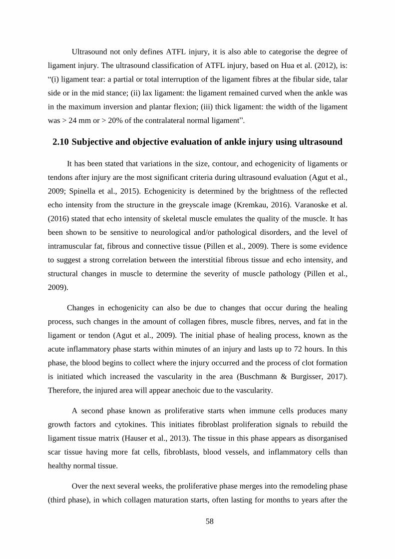
58

Ultrasound not only defines ATFL injury, it is also able to categorise the degree of

ligament injury. The ultrasound classification of ATFL injury, based on Hua et al. (2012), is:

“(i) ligament tear: a partial or total interruption of the ligament fibres at the fibular side, talar

side or in the mid stance; (ii) lax ligament: the ligament remained curved when the ankle was

in the maximum inversion and plantar flexion; (iii) thick ligament: the width of the ligament

was > 24 mm or > 20% of the contralateral normal ligament”.

2.10 Subjective and objective evaluation of ankle injury using ultrasound

It has been stated that variations in the size, contour, and echogenicity of ligaments or

tendons after injury are the most significant criteria during ultrasound evaluation (Agut et al.,

2009; Spinella et al., 2015). Echogenicity is determined by the brightness of the reflected

echo intensity from the structure in the greyscale image (Kremkau, 2016). Varanoske et al.

(2016) stated that echo intensity of skeletal muscle emulates the quality of the muscle. It has

been shown to be sensitive to neurological and/or pathological disorders, and the level of

intramuscular fat, fibrous and connective tissue (Pillen et al., 2009). There is some evidence

to suggest a strong correlation between the interstitial fibrous tissue and echo intensity, and

structural changes in muscle to determine the severity of muscle pathology (Pillen et al.,

2009).

Changes in echogenicity can also be due to changes that occur during the healing

process, such changes in the amount of collagen fibres, muscle fibres, nerves, and fat in the

ligament or tendon (Agut et al., 2009). The initial phase of healing process, known as the

acute inflammatory phase starts within minutes of an injury and lasts up to 72 hours. In this

phase, the blood begins to collect where the injury occurred and the process of clot formation

is initiated which increased the vascularity in the area (Buschmann & Burgisser, 2017).

Therefore, the injured area will appear anechoic due to the vascularity.

A second phase known as proliferative starts when immune cells produces many

growth factors and cytokines. This initiates fibroblast proliferation signals to rebuild the

ligament tissue matrix (Hauser et al., 2013). The tissue in this phase appears as disorganised

scar tissue having more fat cells, fibroblasts, blood vessels, and inflammatory cells than

healthy normal tissue.

Over the next several weeks, the proliferative phase merges into the remodeling phase

(third phase), in which collagen maturation starts, often lasting for months to years after the

59

initial injury (Hauser et al., 2013). With time, the tissue matrix begins to resemble normal

ligament tissue; though, variation in matrix structure persists such as collagen disorganised

and type III collagen becomes more prevalent (Hauser et al., 2013). It seems possible that an

anechoic to hypoechoic appearance of injured ligaments could occur due to the different time

in healing process. However, previous studies just mentioned that the echogenicity became

hypoechoic after injury without stating the time after injury or the stage of healing process.

The three phases of healing process is demonstrated in Figure 2.24.

Figure ‎2-24: Three phases of healing process (inflammation, proliferation, and remodelling)

during acute, sub-acute, and chronic phases

Structural elements in tissues create a reflection and scattering of sound waves which

influence the acoustic impedance of the ultrasonographic image (Agut et al., 2009). The

reflected sound waves (ultrasound echoes) can be transformed to greyscale (Das, 2016) and

the intensity of the returning waves defines the echogenicity of the tissue being scanned. The

echogenicity of ultrasound is generally described by four specific terms (Figure 2.25):

1. Echogenic (or hyperechoic), which involves an increased reflected echo when

compared to adjacent tissue and is appears as white (bright echo) on US images.

2. Hypoechoic, which is a reduced reflection of the echo, appearing as different

shades of darkness (weak echo) on US images.

3. Isoechoic, the echogenicity of the reflected echo is similar to the adjacent tissue.

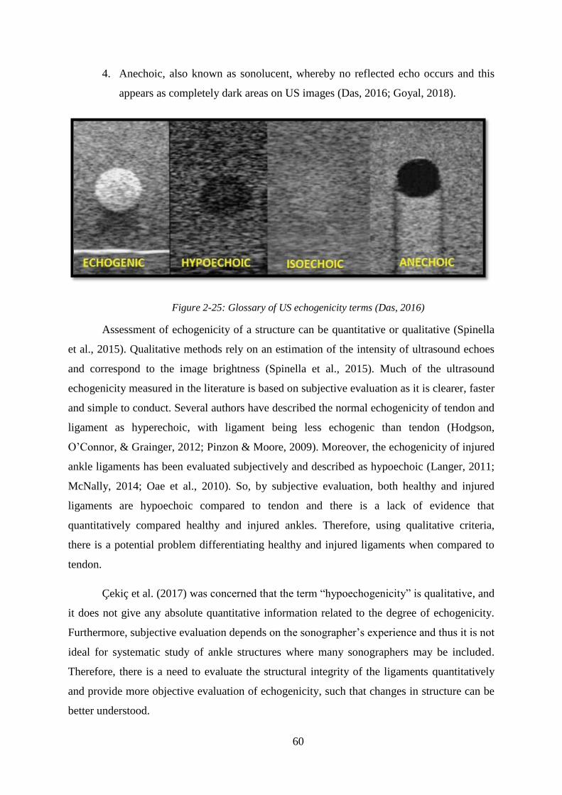
60

4. Anechoic, also known as sonolucent, whereby no reflected echo occurs and this

appears as completely dark areas on US images (Das, 2016; Goyal, 2018).

Figure ‎2-25: Glossary of US echogenicity terms (Das, 2016)

Assessment of echogenicity of a structure can be quantitative or qualitative (Spinella

et al., 2015). Qualitative methods rely on an estimation of the intensity of ultrasound echoes

and correspond to the image brightness (Spinella et al., 2015). Much of the ultrasound

echogenicity measured in the literature is based on subjective evaluation as it is clearer, faster

and simple to conduct. Several authors have described the normal echogenicity of tendon and

ligament as hyperechoic, with ligament being less echogenic than tendon (Hodgson,

O’Connor, & Grainger, 2012; Pinzon & Moore, 2009). Moreover, the echogenicity of injured

ankle ligaments has been evaluated subjectively and described as hypoechoic (Langer, 2011;

McNally, 2014; Oae et al., 2010). So, by subjective evaluation, both healthy and injured

ligaments are hypoechoic compared to tendon and there is a lack of evidence that

quantitatively compared healthy and injured ankles. Therefore, using qualitative criteria,

there is a potential problem differentiating healthy and injured ligaments when compared to

tendon.

Çekiç et al. (2017) was‎concerned‎that‎the‎term‎“hypoechogenicity”‎is‎qualitative, and

it does not give any absolute quantitative information related to the degree of echogenicity.

Furthermore, subjective evaluation depends on‎the‎sonographer’s‎experience‎and‎thus‎it‎is‎not‎

ideal for systematic study of ankle structures where many sonographers may be included.

Therefore, there is a need to evaluate the structural integrity of the ligaments quantitatively

and provide more objective evaluation of echogenicity, such that changes in structure can be

better understood.

61

Many researchers hold the view that quantitative analysis of echo intensity can be

performed through computer-aided greyscale analysis (Arts, Pillen, Schelhaas, Overeem, &

Zwarts, 2010; Çekiç et al., 2017). This method is easily accessible, cheap, safe, more

objective‎ than‎ visual‎ evaluation,‎ less‎ dependent‎ on‎ the‎ examiner’s‎ experience,‎ and‎ allows

statistical analysis (Arts., 2010; Cadore et al., 2012).

Several authors have introduced quantitative methods including mean echogenicity to

objectively evaluate musculoskeletal ultrasound images. Prior reports have focused on digital

flexor ligaments and tendons of metacarpal area in horses, through analysis of greyscale areas

within images (Agut et al., 2009; Spinella et al., 2015; Vergari et al., 2012). Cheng and

colleagues (2012) studied the reliability of measuring the echogenicity of the human foot

plantar fascia quantitatively by measuring the mean greyscale of their specific area of

interest. They demonstrated that the reliability of greyscale assessments of echogenicity was

high to very high (ICC ranged from 0.76 to 0.94). It was concluded that calculating the mean

greyscale could reduce inconsistencies in the interpretation of echogenicity among different

sonographers (Cheng et al., 2012). It has been reported recently that quantitative ultrasound

techniques have the ability to provide quantitative evaluation of the structure and function of

musculoskeletal tissues (Wang, Huang, Yeow, Pickering, & Saarakkala, 2017) and computer-

aided image analysis software has been widely used for ultrasound images.

ImageJ is Java-based computer-aided image analysis public domain software

developed by the National Institutes of Health (Bethesda, MD, USA). The effectiveness of

using ImageJ has been shown with thyroid, breast, uterus, and muscles imaging (Arts et al.,

2012; Çekiç et al., 2017; Chou et al., 2011; Grani et al., 2015; Watanabe et al., 2013). The

quantification of the echo intesity in ImageJ has been made using grey-level histograms,

which demonstrates the distribution of the pixels in the ultrasound image by plotting the

number of pixels at each level of colour intensity (Figure 2.26). Santos and Armada-da-Silva

(2017) found moderate to very high reliability of measuring the echo intensity of the

quadriceps femoris muscle by using histogram analysis in ImageJ.

62

Figure ‎2-26: Image analysis region of interest selections and the corresponding greyscale

histogram values. Yellow rectangular represented the region of interest of the longitudinal image of

rectus femoris. The corresponding greyscale histogram showed the mean echo (Harris-Love, Seamon,

Teixeira, & Ismail, 2016)

Hsu and colleagues found that grey-level histogram of ultrasound images is a

promising method which was sensitive to differences in participants with tendinopathy.

Moreover, Erol et al. (2013) reported that the histogram analysis provides quantitative

information regarding the echogenicity of the breast tissue. Chou and colleagues (2011)

showed that grey-level histograms were useful in evaluating the physiological condition of

the endometrium (Chou et al., 2011).

Çekiç et al. (2017) studied echo intensity in patients with Hashimoto thyroiditis and

concluded that greyscale histograms provide objective and quantitative information regarding

the echogenicity of the thyroid parenchymal. Histogram analysis was also able to

differentiate between normal and heterogeneous parenchyma. Moreover, Grani and

colleagues (2015) used histogram analysis to evaluate the echogenicity of thyroid nodules,

finding they were able to quantify the degree of hypoechogenicity (Grani et al., 2015). Erol et

al. (2013) concluded that lesion echogenicity ratio measured by greyscale histogram can be

utilised as an adjunct ultrasound parameter to discriminate between malignant and benign

breast lesions.

A number of previous studies have quantified echo intensity to describe the quality of

muscle (Arts et al., 2012; Cadore et al., 2012; Mangine et al., 2014; Watanabe et al., 2013).

Arts et al. (2012) conducted an ultrasound study on nine different muscles in a patient with

amyotrophic lateral sclerosis (ALS). The echogenicity was measured as the mean greyscale

value of the muscle, expressed as a value between 0 (black) and 255 (white). They concluded

63

that the echogenicity of all muscles (range 52-91) in ALS patients was almost twice the

normal value (28-42). They compared their findings with the post-mortem histopathological

examination of an older woman who had had ALS and found that fibrous tissue was the main

contributing factor to increase the echogenicity of the muscle (Arts et al., 2012). Furthermore,

Watanabe et al. (2013) conducted a study to investigate if the quality of the muscle, based on

echogenicity, is related to muscle strength independently of muscle size in elderly men.

Echogenicity of the rectus femoris muscle was measured by greyscale analysis, utilising the

standard histogram function and a significant negative correlation was found between

echogenicity and muscle strength (Watanabe et al., 2013).

However, the existing literature on echo intensity in musculoskeletal ultrasound

focused particularly on plantar fascia and muscles. There has been little quantitative analysis

of the specific echogenicity of the tendons and ligaments around the foot and ankle. To the

author’s‎ best‎ knowledge,‎ no‎ study‎ has‎ quantitatively evaluated the echo intensity of the

ATFL in healthy, coper, and CAI participants. It is believed that a precise knowledge of

tendon and ligament echogenicity reference values for specific structures may serve as a tool

to distinguish between physiological and abnormal cases (Agut et al., 2009; Spinella et al.,

2015).

Whilst the measurement of foot and ankle structures can characterise structural

changes, it does not provide any insight into the functional consequences of any such

changes. People with CAI present with impairment such as pain, loss of function, and

restricted motion that affect the daily living activity in general population and athletic

participation (Pope et al., 2011). It has been thought that CAI is related to ligamentous and

soft tissue damage to the lateral ankle structures and is further confounded by changed

muscle activation, limited range of motion, and balance deficits (Arnold, De La Motte,

Linens, & Ross, 2009; Hertel, 2008; Hoch et al., 2016).

2.11 Ankle injury and postural control

Several researchers hold the view that individuals with a history of ankle sprains are

at a high risk having another ankle sprains or CAI (Engebretsen et al., 2009; Trojian &

McKeag, 2006; Naja et al., 2017; Steffen et al., 2008), with 47% of recurrent ankle sprain

occurring in the same ankle that had been already sprained (Trojian & McKeag, 2006). Many

factors are thought to contribute to the reoccurrence of an ankle sprain such as: limited

64

mobility of the ankle joint, weakness of the ankle muscles, and damage to the proprioceptors

in the ankle ligaments (Akbari, Karimi, Farahini, & Faghihzadeh, 2006). Proprioceptors exist

through ligaments, tendons, and muscles and provide sensory information for the control of

balance (Chae, Kim, & Lee, 2017). Balance is the ability‎ to‎maintain‎ the‎body’s‎ centre‎of‎

mass within the base of support (Greenfield, 2014) and postural sway is the movement of the

centre of mass when standing, and reflects the control of balance (Cho, Lee, Lee, Lee, & Lee,

2014).

A systematic review found that postural control is impaired following an acute lateral

ankle sprain (McKeon & Hertel, 2008b), specially for those with CAI (Arnold, De La Motte,

Linens, & Ross, 2009; Gribble, Hertel, & Denegar, 2007; Hiller, Kilbreath, & Refshauge,

2011; Mettler et al., 2015). Deficiencies in postural control are thought to arise because of a

combination of diminished proprioception (the cumulative neural input to the CNS from

mechanoreceptors in the joint capsules, ligaments, tendons, muscles, and skin) and

neuromuscular control (the efferent response that is generated as the consequence of the

proprioceptive afferent input) (Hertel, 2002; Voight & Cook, 2014).

Deficits in the pattern of lower extremity muscle activation have been assume to be

contributing factor to impairments in postural stability and perceived function in people with

CAI (Webster, Pietrosimone, & Gribble, 2016). Delahunt et al. (2006), for example, found

that CAI participants had less anticipatory activation of peroneus longus during a unipedal

drop jump compared to control participants. They suggested that this alteration in motor

control could contribute to the risk of further inversion injuries in cases of CAI. Previous

studies comparing neuromuscular control between coper and CAI participants found that

copers demonstrated increased activation of peroneus muscle during jump landing (Gutierrez

et al., 2012), and tibialis anterior during pre- and post- touchdown phases of gait (Dundas,

Gutierrez, & Pozzi, 2014). The researchers concluded that copers may have developed these

adaptive strategies as a protective mechanism to prevent further injury. However, more

researches need to support this conclusion. This again points to cases of CAI having a

neuromuscular control basis to the risk of further injury.

Damage in any part of afferent or efferent controls could create postural control

deficiency.‎Proprioception‎is‎defined‎in‎the‎literature‎as‎one’s‎ability‎to‎integrate‎the‎sensory‎

signals‎ from‎ many‎ mechanoreceptors‎ to‎ thereby‎ set‎ the‎ body’s‎ movement‎ as‎ well as its

position, in space (Goble, 2010; Han, Waddington, Adams, Anson, & Liu, 2016). It has been

65

stated that ankle proprioception is probably one of the most significant contributor to control

of posture, particularly in sport, since the ankle-foot complex is the only segment of the body

touching the ground in most of sports activities (Han, Anson, Waddington, Adams, & Liu,

2015). Furthermore, ankle proprioception and control give vital information and stability that

allows modification of the upper body in order to effectively achieve the complex motor tasks

needed in many sports (Han et al., 2015). A systematic review conducted on balance ability

and the performance of athletes found that balancing abilities of ice hockey players

demonstrates a significant association with extreme skating speed (Hrysomallis, 2011).

Furthermore, a study in male athletes from various sports involving jumping and landing

(basketball, handball, volleyball and soccer) found balancing ability was significantly

associated with the‎athletes’‎agility‎ (Sekulic, Spasic, Mirkov, Cavar, & Sattler, 2013). This

evidence supports a hypothesis that controlling balance is essential for the performance of

sport activities (Han et al., 2015) and thus the role of the ankle in postural control, and how

ankle injury impacts this role, is pertinent to understanding risk of lateral ankle sprains.

2.11.1 Strategies of postural control

The strategy of postural control can be either compensatory (reactive) or anticipatory

(predictive) or a combination of both (Pollock, Durward, & Rowe, 2000). An anticipatory

postural control strategy could include a voluntary movement, or increase in the activity of

the muscle in anticipation of a predicted disturbance (Pollock et al., 2000). A movement or

muscular response after unpredicted/unexpected disturbance is known as compensatory

postural control strategy. These responses may involve a “fixed-support”,‎ in‎which the base

of support remains unchanged but the location of the centre of mass is‎moved,‎or‎“change-in-

support”‎in‎which‎the‎base‎of‎support is altered so that the centre of mass remains within it

(Pollock et al., 2000).

Postural control is based on continues integration of sensory information from visual,

vestibular, and somatosensory receptors (mechanoreceptor and proprioceptors). The CNS

gathers and processes this sensory information from the receptors in the joints, tendons,

ligaments, and muscles to gauge the motion and the position of limbs (Mills, 2018). Modig

(2013) reported that postural control as a constantly ongoing process which cycles through

corrective feedforward (predictive) and feedback (reactive) regulative movement control

systems (Figure 2.30). For instance, when the body sway from upright position, it generates a

passive torque around the ankle joint because of the acceleration of the body due to gravity.

66

This information is transmitted to the brain from the joint and muscles in the form of sensory

feedback, thereafter a corrective, active torque is applied to maintain balance (Cnyrim et al.,

2009). Disturbance of any of these sensory inputs due to injury create a change in the control

of balance, reflected experimentally in postural sway (Clark, Treleaven, & Ulrik, 2015; Serra-

AÑó, López-Bueno, García-Massó, Pellicer-Chenoll, & González, 2015).

Figure ‎2-27: Human postural control

In case of single-leg balance, the participants foot’s‎supinate‎and‎pronates‎to maintain

the body centre of mass above the base of support which defined as‎ ‘ankle‎ strategy’ of

postural control (Hertel, 2002). CAI participants on the other hand have been shown to rely

more‎on‎‘hip‎strategy’‎to‎maintain‎single‎limb‎balance‎than‎healthy‎participants,‎this‎strategy‎

assumed to be less efficient than ankle strategy (Hertel, 2002; Pintsaar, Brynhildsen, &

Tropp, 1996).

2.11.2 Measuring postural stability

Postural control can be categorised into three states: static with the goal of

maintaining position with an insignificant level of movement; semi-dynamic with the goal of

maintaining position by moving the base of support; or dynamic with the goal of maintaining

a fixed base of support by performing a given movement (Hosseinimehr, Daneshmandi, &

Norasteh, 2010; Pionnier et al., 2016).

67

Evaluation of static postural control can be measured with instrumented tool such as

force plate or reliable and valid clinical scale such as Balance Error Scoring System (Gribble,

Hertel, & Plisky, 2012). Even though measuring the postural control through static test

provides valuable clinical information, the original task of maintain standing may not

translate certainly to movement tasks that occur in physical activity (Gribble et al., 2012). On

the other hand, dynamic types could include performing an action such as jumping or

hopping to a different place then instantly trying to stay as still as possible, or trying to

perform decided segment movements (reaching) without compromising the established base

of support (Gribble et al., 2012). Dynamic single-leg jump-landing test and the SEBT are

alternative evaluation methods that might challenge balance more than single-leg static

balance test (Arnold et al., 2009). Even though performing these dynamic actions to evaluate

postural stability do not precisely replicate participation in daily activity and sport, they more

closely imitate the demands of physical activity than evaluating postural stability in static

way (Gribble et al., 2012). A meta-analysis study demonstrated that all of dynamic measuring

outcomes are able to exhibit the balance deficits in CAI individuals (Arnold et al., 2009)

while de Vries and colleages (2010) found that there was no statistical significant difference

in the measurements of static balances between healthy, participants shortly after acute ankle

sprain and participants with CAI. Dynamic balance tests could provide an overall evaluation

of joint stability, strength, sensorimotor function, which could assist clinicians detect balance

deficits that would not be identify with static tests. Time to stabilisation is an another

dynamic task that evaluates how long the participant takes to return the ground reaction force

to a stable range. It measured during landing from a single-leg jump (Brown & Mynark,

2007; Ross, Guskiewicz, Yu, Carolina, & Hill, 2005; Dallinga et al., 2016). Time to

stabilisation test needs force plates and specific processing software to produce the measures.

This makes time to stabilisation less convenient to use clinically than SEBT (Arnold et al.,

2009).

Dynamic evaluation such as SEBT may be preferable and able to provide a more

precise evaluation of the function of lower extremities in people with CAI than static

evaluation which involves only quiet standing, the SEBT needs greater demand from an

individual and therefore more sensitive to picking up differences in balance compared to the

static (Razeghi, Rahnama, & Shokri, 2016). Two systematic reviews have revealed that

stability differences could not be detected through static balance tasks because they may not

68

be sensitive enough to detect minor variances in postural control (McKeon & Hertel, 2008b;

Wikstrom, Naik, Lodha, & Cauraugh, 2010).

2.11.2.1 Star excursion balance test (SEBT)

SEBT has been known as the extent to which the participant can reach without lifting

their feet and staying stable. SEBT was first used by Gray as a clinical treatment method

(Gray, 1995), since then it has been applied as an objective measurements for dynamic

postural control, and utilised as a diagnostic task to determine risk of injury, and to

discriminate pathological conditions (Anderson, 2016). The performance of the SEBT

provides a quantitative evaluation, with the reach distance in centimetres is the main outcome

measure for clinical and research setting. This outcome is normalised to leg length to

facilitate the comparison between people (Gribble & Hertel, 2003). The quantitative

evaluation of the reach distance by either absolute value (cm) or normalisation (%) has many

valuable purposes as it produces normative data, which will permit for ranking for statistical

means, determines risks of injury, and monitors consequence of interventions (Anderson,

2016; Gribble, Hertle, & Plisky, 2012). Moreover, it has been thought that SEBT is an

excellent representor for functional activity among other postural control tests options since it

integrates a combination of flexibility, strength, and neuromuscular control while challenging

the limits of postural stability (Hoch et al., 2016).

Several authors have proposed that by performing SEBT, participants challenge their

limits of stability while trying to reach as far as they can, thereby revealing to some degree of

their dynamic postural stability (Dallinga et al., 2016; Gribble et al., 2012; Hoch et al., 2016).

First, performing SEBT requires greater strength than quiet standing tasks. A recent study

found that isometric hip strength in participants with CAI significantly influenced the

performance of dynamic balance, with abduction and external rotation explained almost 25%

of the SEBT score during the posterolateral and posteromedial directions respectively

(McCann et al., 2017). Moreover, in order to achieve the goal of SEBT, closed kinetic motion

at the ankle, knee, and hip should effectively controlled by the musculature of the lower limb

(Olmsted, Carcia, Hertel, & Shultz, 2002). On the other hand, keeping a single-leg stance

while standing-up on a steady platform puts a quite a small strength demand on the lower

extremity musculature (Olmsted et al., 2002). Second, performing SEBT requires a greater

range of motion than static tasks do. Keeping one leg stable while reaching a specific point

with the other leg requires the stable leg to be capable of adequate motion of the ankle, knee,

69

and hip (Olmsted et al., 2002). Anderson (2016) used SEBT to measure the functional joint

mobility and found that ankle dorsiflexion of healthy participants was correlated with

normalised reach distance in the SEBT. Moreover, Kang et al. (2015) hypothesised that

kinematics of the lower extremity would be strong predictors for the reach distance of the

SEBT (anterior, posteromedial, and posterolateral). They found that ankle dorsiflexion was

the best predictor of normalised reach in the anterior direction.

The SEBT is a simple, low-cost, reliable (ICC was 0.95 and 0.98 for intra-rater and

inter-rater respectively) alternative to sophisticated instruments that measure the functional

performance of a lower limb (Hyong & Kim , 2014; Khuman et al., 2014). SEBT is designed

to challenge postural stability during various leg reaching tasks and has recently gained

increased attention in research and clinical areas (Doherty et al., 2015a). It is theorised that

SEBT may predict lower extremity injuries. Plisky, Rauh, Kaminski, and Underwood (2006)

demonstrated that the SEBT was able to predict a 2.5 times greater chance sustaining a lower

extremity injury if the difference between right and left anterior reach distances greater than 4

cm. De Noronha et al. (2013) reported that participants with SEBT posterolateral under 80%

were at 48% greater risk of having ankle sprain. One possible explanation the only

posterolateral direction may predict the incidence of ankle sprains is rely on the variation of

muscle activation patterns that my impose for each direction.

The reliability of SEBT in assessing dynamic balance was first established by Kinzey

and Armstrong in 1998. Furthermore, four studies have since shown the high reliability of the

SEBT in measuring dynamic balance capability in participants with and without chronic

ankle instability (Hertel, Miller, & Denegar, 2000; Hoch, Staton, & McKeon, 2010; Hyong &

Kim, 2014; Munro & Herrington, 2010). Hertel et al. (2000) evaluated the intra-rater and

inter-rater reliability of SEBT in 16 healthy athletes. The ICC of the intra-rater was up to 0.96

on both days and the ICC of inter-rater was up to 0.84 on day 1 and up to 0.93 on day 2.

Hyong and Kim (2014) also evaluated the inter-rater and intra-rater reliability of SEBT in 67

healthy participants. The ICC of inter-rater was up to 0.95 and the ICC of intra-rater

reliability was up to 0.98. They concluded that SEBT is a highly reliable test that can be used

to measure dynamic balance (Hyong & Kim, 2014). In addition, Olmsted et al. (2002) argued

that SEBT is the first non-instrumented functional test that has been demonstrated to be

greatly sensitive and reliable in determining the deficits between healthy participants and CAI

participants. The test-retest reliability of modified SEBT (known as Y-balance test) was

determined by Hoch et al. in 2010.The researchers concluded that the test has good reliability

70

to evaluate the dynamic postural control in a CAI group, and the anterior direction has the

highest reliability followed by posteromedial and posterolateral (ICC = 0.92, 0.86, 0.74

respectively).

Plisky et al. (2006) assessed the between-session reliability of the SEBT on basketball

players and found ICC values ranging from 0.84 to 0.87. However, they used a Y-balance test

containing only anterior, posterolateral and posteromedial directions. Therefore, Munro and

Herrington (2010) assessed the between-session reliability of the eight directions of the

SEBT. The ICC ranged from 0.84 to 0.94 and the authors concluded that SEBT is a reliable

measure in healthy recreational athletes to determine their lower limb function (Munro &

Herrington, 2010). There is a lack of reliability of the eight directions of the SEBT in people

with CAI since most of the reliability studies that have been done previously were on healthy

participants.

In addition to the positive reporting regarding the reliability of SEBT discussed

above, it has also been reported that SEBT is effective in detecting the dynamic type of

postural control in both healthy and CAI participants (Khuman et al., 2014). The process of

performing the test is easy to understand and easy to apply, with minimal equipment required

(Khuman et al., 2014). Furthermore, the body of evidence reveals that SEBT is a functional

clinical test that is widely used in ankle disorders such as acute lateral ankle sprain (Doherty

et al., 2015b).

However, the SEBT can often be time-consuming and take approximately 45 minutes

to complete (Munro & Herrington, 2010). It is recommended that subjects complete six trials

in each direction (eight directions in total) and then taking another three recorded trials

(Hertel et al., 2000). Hertel et al. (2000) recommended applying six practice trials due to a

significant learning effect across trials one to six, with the most consistent scores and longest

reach distances from trials seven onwards. Significant learning effects were seen between

trials seven-nine and one-six (p<0.05). Moreover, Hertel et al. (2000) protocol allowed

participants to use their arms for balance, which is not in line with the most common SEBT

protocol which is that hands should remain on hips. These two factors could increase the

learning time for the tasks (Munro & Herrington, 2010). Khuman et al. (2014) followed

Hertel’s‎ recommendation and applied six practice trials in all eight directions. Even though

six practice trials were recommended, several authors considered the problems associated

with‎Hertel’s‎protocol‎and‎reduced‎the‎number‎of‎trials to five (Akbari et al., 2006). Robinson

71

and Gribble (2008b) conducted a study of the longest normalised reach distances to define the

precise numbers of trials required for stabilising scores. The results of the study demonstrated

that the lateral direction was the only direction which required more than four practice trials

before constancy was achieved on the fifth trial. The researchers established that only four

practice trials are required before the baseline measuring reaches distances suitable for

research or clinical purposes. Hoch and colleagues (2016) also asked their subjects to perform

four practice trials and then three recorded trials, taking the average of the three recorded

ones for analysis. Similarly, Pionnier et al. (2016) asked their participants to get familiar with

the test by performing four practice trials and then one recorded trial. However, Payne,

Mccabe, and Pulliam (2016) reduced the trials in performing SEBT to three trials, and

averaged these for data analysis. Their study had the ability to identify the differences in

postural control between healthy and CAI participants. Therefore, it appears that applying

SEBT can be simplified by using fewer practice trials (Munro & Herrington, 2010).

In addition to reduce the number of trials to minimise the time required to do the

SEBT, researchers built the Y-balance test (YBT) which based on previous research

suggesting redundancy in the eight directions of the SEBT in order to reduce the time

required to do the SEBT and to decrease the development of fatigue. Pilsky et al. (2006)

applied‎Y‎or‎“peace‎sign”‎including‎anterior,‎posteromedial,‎and‎posterolateral‎directions‎as‎a‎

predictor of lower extremity injury in high school basketball players, which in turn led to the

development of the YBT.

It has been demonstrated in the literature that individuals with acute ankle sprain and

CAI achieved shorter reach distance on the SEBT than individuals without sprain (Brown,

Bowser, & Orellana, 2010; Doherty et al., 2015a; Gribble et al., 2007; Jaber et al., 2018;

Hertel, Braham, Hale, & Olmsted-Kramer, 2006; Pionnier et al., 2016; Plante & Wikstrom,

2013). Olmsted et al. (2002) was the first to conducted a study on 20 healthy participants and

20 with unilateral CAI, and found that participants with CAI revealed significantly shorter

reach distances from healthy when standing on the injured limb (78.6 cm versus 82.8 cm). In

their analysis, the eight reach distances from all SEBT directions were averaged together. The

lateral direction had the shortest reach distances in comparison to the other seven directions,

followed by the anterolateral direction, which was shorter than the other directions except the

lateral. Furthermore, no joint kinematics were tested, leaving the explanation of the result

difficult. In addition, Olmsted et al. (2002) did not normalise the reach distances to the

subjects’‎leg‎lengths‎with‎average leg length of CAI participants was 2 cm lower than healthy

72

participants; instead, they matched the height and leg length for both healthy and CAI groups

as closely as possible. A study by Gribble & Hertel (2003) which recruited 30 recreationally

active subjects was designed to test the role of leg length and height on reach distances while

performing the SEBT. The findings were that height and leg length were strongly correlated

with reach distances, with leg length displaying a stronger correlation than height (Gribble &

Hertel, 2003). Therefore, the authors recommended that the result for reach distance should

be normalised to leg length (Khuman et al., 2014; Payne et al., 2016).

Akbari et al. (2006) examined the differences in reach distance in 30 athletes with

unilateral acute lateral ankle sprains. Even though their results showed a significant

difference in reach distance in injured limb and uninjured limb (84.97±10.26 cm and

86.80±9.34 cm respectively), they fail to specify which reach directions they applied. In

addition, authors did not compare the result with healthy participants as they assumed that the

uninjured limbs are healthy. However, Doherty et al. (2015a) found decrease normalised

reach distance on the injured and noninjured limbs of people with 6 months after acute lateral

ankle sprain during the performance of the YBT. In addition, Hiller et al. (2008) reported that

previous ankle sprain could predispose both ankles for sustaining an ankle sprain, therefore, it

seems important to compare the injured ankle of CAI participants with a healthy ankle in

participants who never expose to ankle sprain.

Applying normalised reach distances, Gribble and colleagues (2004) found a

decreases reach distance in CAI on their injured side in the three directions of the SEBT

(anterior, medial, and posterior). Khuman et al. (2014) also used SEBT to compare dynamic

postural control between 30 healthy and 30 CAI participants. The results of their study agreed

with‎ Olmsted’s‎ results,‎ as‎ they‎ found‎ that‎ the‎ reach‎ distance‎ of‎ CAI‎ participants‎ was‎

significantly lower than that of the control participants, and lateral and anterolateral

directions had the shortest reach distances. In addition, the injured limb in CAI participants

has the lower reach distance compared to the uninjured limb (p<0.01), and no significant

differences were reported between dominant and non-dominant injured limbs (p>0.05)

(Khuman et al., 2014). Recently, Pionnier et al. (2016) applied a new approach to SEBT

which aimed to evaluate dynamic postural control in 17 healthy and 17 participants with CAI.

They used an optoelectronic cameras system as a more accurate method to assess the reach

distances. In addition to measure the lower limb range of motion (ROM), they computed new

relevant variables, such as the absolute time required to reach each distance. The main

outcome was a significant difference in reach distances between the two groups; that

73

participants complaining of CAI reached 80% of leg length while the healthy participants

reached 85% of leg length. However, the authors reported the average of the reach distance

for all 8 directions (Pionnier et al., 2016). Even though the authors used a different approach

to evaluate postural control, the results of the three studies were consistent. Pionnier et al.

(2016) also found that a shorter time was needed to perform the test in CAI participants even

there was a lack of statistically significant difference between CAI and healthy participants.

Furthermore, the authors demonstrated a significant decrease in the ROM of lower limbs joint

(ankle, knee, and hip) and the velocity of the centre of pressure (p<0.05) in the CAI

participants compared to healthy participants. These decreased quantitative performance

highlighted a deficit in dynamic postural control.

In contrast to earlier findings, Hertel et al. (2006) evaluated the SEBT in 48 adults

with CAI and 39 controls and suggested that the reach distances in the posteromedial, medial,

and anteromedial directions were significantly lower in CAI compared to the controls, and

that the posteromedial direction was the highly associated with the performance of the eight

directions in the CAI group. In addition, they recommended that these three directions may

be clinically utilised to evaluate the functional deficits associated with CAI. However, the

clinical implications of these three specific medial reach directions are not clear and needs

additional study.

Following the recommendation of Herterl et al. (2006), Sefton et al. (2009) used the

three medial directions of the SEBT as a measurement tool to understand the role of

sensorimotor impairment in participant with chronic ankle instability. Their result showed no

statistically significant differences in the three reach distances between control and CAI

participants. It seems possible that this result is due to the variety of activity level between

the groups. CAI participants spend more years on sport competition than healthy participants.

Many of CAI participants had a high level of activity which indicates these participants are

promoting coping mechanisms to deal with their disability (Sefton et al., 2009). Conducting a

study on very homogeneous people might be more possible to create significant differences

between healthy and chronically unstable ankles. In addition, De La Motte et al. (2015) found

no differences between CAI and healthy participants. Researcher only examined the three

medial directions. It seems that the three medial directions could not be the most sensitive to

CAI related achievement deficits.

Several authors used YBT which contains only three reach directions (anterior,

posteromedial, and posterolateral) instead of the eight directions of the SEBT in their studies.

74

Payne et al. (2016) studied the effect of CAI on the Y-balance test among soccer players and

found that the differences in reach direction between healthy and CAI participants was only

demonstrated in the anterior direction. The study compared only 15 injured subjects to 59

healthy ones; the sample sizes were therefore not equal, which may have affected the results

of the study. Plante and Wikstrom (2013) found a significant decreased normalised reach

distance in only posteromedial direction in CAI participants compared to coper and healthy,

no differences were found between coper and healthy participants. A recent study

demonstrated a poorer dynamic balance performance mostly during the anterior direction of

YBT between the three groups (healthy, coper, and CAI) with CAI group had the lowest

reach distance during the anterior direction and no significant differences was observed

between copers and healthy groups (Jaber et al., 2018).

A possible explanation of the conflicting results between the studies regarding the

affected reach direction is that each reach direction could activate the stance lower extremity

muscles to different extent. Earl and Hertel (2001) measured the EMG (electromyography)

activity of different muscles (gastrocnemius, anterior tibialis, biceps femoris, medial

hamstring, vastus lateralis, and vastus medialis oblique) during the performance of all eight

directions of the SEBT. The authors found that all muscle activity is reach dependant except

the gastrocnemius. Feger and cholleagues (2014) found a significantly less anterior tibialis

muscle activity duting the anterior and posteromedial reach directions in the CAI participants.

Jaber et al. (2018) found less anterior tibias and gluteus maximus activation in CAI

participants compared to coper and healthy participants during the anterior and posterolateral

direction of the YBT, which could demonstrate a relationship between altered neuromuscular

control at the hip and ankle and the performance of the YBT. Posterolateral is challenging

reaching direction, as participants need to maintain a level pelvis on the stance leg. As

participants reach backward across the stance leg, they shift their trunk anteriorly to keep the

centre of mass within the base of support. Trunk flexion creates hip flexion moment that is

controlled by the contraction of hip extensors. Therefore, increased gluteus maximus

activation could be required in this case to counteract the sagittal plane flexion of the hip and

trunk. It seems that CAI participants did not fire the gluteus maximus as it needs to

counteract‎this‎motion,‎resulting‎in‎overcompensation‎to‎maintain‎the‎body’s‎centre‎of‎mass‎

within the base of support, which could lead to create a higher sway in the posterolateral

direction (Jaber et al., 2018).

Furthermore, Razeghi et al. (2016) examined the ability of the YBT to discriminate

between female athletes with and without CAI. Their findings contradicted the previous

75

findings, as no statistically significant differences were found in any of the reach distances

between the CAI and control groups. They concluded that the YBT may not be sensitive

enough to determine balance deficiency between athletes with and without CAI (Razeghi et

al., 2016). However, the study was conducted on female athletes and from inhomogeneous

population from various types of sport such as: basketball, volleyball, and handball, which

may affect the finding.

There is a lack of consistency in inclusion and exclusion criteria, and methods within

the literature therefore making it difficult to compare studies. Subjects exist possibly along a

continuum of instability and may display more or less disability than participants in other

studies. This is evidenced by the difference in self-reported number of sprains and scores on

functional questionnaires. Each study used different types of questionnaires to evaluate the

level of ankle dysfunction such as CAIT, FADI, and AJFAT. Moreover, there are various

level of function with different activities and differences in the number of episodes of giving

way (Brown et al., 2010). These differences are likely to produce different definitions of

groups.

A study conducted by Coughlan and colleagues (2012) debated that different postural

control strategies are employed during the traditional YBT compared to the commercial

YBT. In other words, variations in selected reach directions and the way the test was

performed may also play a role in the differences among the findings. This notion is

supported by Coughlan et al. (2012) and Fullam, Caulfield, Coughlan & Delahunt (2014),

who found differences in the anterior reach distance between the SEBT and YBT well as

angular displacement in sagittal plane of the hip joint at the point of maximum reach.

Coughlan et al. (2012) measured the SEBT reach directions by attaching three measuring tape

to the floor, one placed anteriorly toward the apex and the remaining two placed at 135º to

the one line in the posteromedial and posterolateral directions. The Y-balance test was

measured by commercially available device (Y Balance Test, Move2Perform, Evansville, IN,

USA). The differences could be that each test presents different mechanism of feedback and

feedforward control. During the SEBT, participants place downward pressure through the

reach foot at the end of the reach excursion only, thus, do not receive same level of afferent

information throughout the movement, possibility depend on feedforward control technique

till the toe touched the measuring tape. While participants in Y-balance test, need to stand in

an elevated position on a central footplate and pushing a sliding block. Therefore, participants

receive constant proprioceptive feedback through the reach excursion from the plantar

76

surface of the reach foot (Coughlan et al., 2012). Thus, researcher should be careful when

interpreting the reach distance from both tests specially the anterior direction.

It seems important to exam the eight directions of the SEBT not only YBT because of

the different findings in reaching directions which have been found between using the eight

directions of the SEBT and YBT. In addition, Plisky et al. (2006) did not mention as to why

they selected the posterolateral as one of the three, and not any other reach directions.

Furthermore, several studies have found significant difference in reach distance in CAI

compared to healthy in directions other than YBT (Hertel et al., 2006; Khuman et al., 2014;

Pionnier et al., 2016).

Authors suggested future research of measuring dynamic postural stability should

include kinematics to assist define mechanisms which could give an idea about the strategy of

the movement and the original of deficiency which cause the poor performance in the SEBT

in particular individuals (Olmsted et al., 2002). Recognising those mechanisms can assist in

improving rehabilitation programs.

2.11.2.2 Ankle kinematics

Although the reliability and validity of the SEBT have been recognised previously,

this test is remarkable in that a hypothetically several types of strategies may be utilised to

achieve the movement goal and produce a similar result (Gribble et al., 2013). It has been

believed that biomechanical assessment of dynamic balance in individuals with lateral ankle

sprain while performing the SEBT may provide insight into the strategies and mechanisms by

which individual progress to fully recover or develop another sprain (Hoch et al., 2016). This

aspect of the SEBT has sparked many researchers with the aim of testing the kinematics that

being a part to an efficacious achievement of this task (Hoch et al., 2016).

Biomechanical measurement of lower limb kinematics during the SEBT has been

limited mostly to sagittal plane. Robinson and Gribble (2008a) tested the lower limb

kinematics of 20 healthy participants while performing the SEBT by using an

electromagnetic tracking system. They found that hip and knee flexion account for 62-95% of

the difference in the reach distance. However, they did not test the dorsiflexion of the ankle

joint, which has been shown to be the greatest sagittal plane contributor to maximal anterior

reach distance in healthy participants (Fullam, 2014). During maintain balance in a close

kinetic chain, the ankle goes into dorsiflexion when the proximal part of tibia moves forward,

forcing the knee into flexion (Hoch, Staton, & McKeon, 2011). This could overestimate the

77

results presented by Robinson and Gribble (2008a) about the strong prediction of the hip and

knee flexion on the reach distance, by not including ankle motion in the equation. In addition,

Hoch and colleagues (2011) found a significant correlation between the dorsiflexion ROM of

the ankle joint (measured during a WBLT; weight-bearing lung test) and reach distance of

YBT only on anterior direction among healthy participants. They proposed that dorsiflexion

ROM accounted for approximately 28% of the alteration in anterior direction (Hoch et al.,

2011) and concluded that WBLT elucidated a significant percentage of the alteration in the

anterior reach distance. Thus, the anterior reach distance of the SEBT can be a good clinical

test to evaluate the impacts of dorsiflexion limitations on dynamic balance and sagittal plane

kinematics of lower limb seems to be the most influence to the performance of SEBT.

However, the previous mentioned studies conducted on healthy participants only, and most of

them measured only three out of eight directions of the SEBT, therefore it is unclear the

contribution of ankle kinematics on other directions of the SEBT.

Wikstrom and Hubbard (2010) found that talar position was significantly more

anterior in injured CAI participants compared to healthy participants which could explained

the restrictions in posterior talar glide in participants with previous ankle sprain. Changed

joint arthrokinematics could contribute to observed decrease in ankle dorsiflexion ROM

(Wikstrom & Hubbard, 2010).

The degree of ankle dorsiflexion plays a role in the risk of lower extremity injuries

(Backman & Danielson, 2011; Drewes, McKeon, Casey Kerrigan, & Hertel, 2009). The

limitation of ankle dorsiflexion ROM after lateral ankle sprain has been considered a

predisposing factor for ankle sprain reoccurrence because decreased dorsiflexion prevents the

ankle from reaching its closed-pack position by holding the ankle in a hyper-supinated

position (Terada, Harkey, Pietrosimone, & Gribble, 2014). A systematic review by De

Noronha et al. (2006) supported the relationship between dorsiflexion and ankle sprain. There

are several techniques have been used in the research and clinical settings to measure the

dorsiflexion range of motion associated to ankle injury such as goniometers and

inclinometers. However, these approaches depends on the technique which used by the

examiner during the test (Almansour, 2015). A WBLT has also been used to measure the

dorsiflexion and demonstrated high reliability with an ICC of 0.99 (Konor, Morton,

Eckerson, & Grindstaff, 2012). Doherty et al. (2015a) measured the ankle dorsiflexion ROM

between participants six months after their acute lateral ankle sprain and healthy participants

by using the WBLT and found no differences between the two groups. However, they found

significant decrease of ankle dorsiflexion in the acute lateral ankle sprain groups while the

78

performance reach directions of YBT by using 2D video analysis. Since the WBLT

demonstrated a similar ankle dorsiflexion between the two groups and the YBT demonstrated

differences in ankle dorsiflexion between the groups, the authors speculated that the

compensatory movement of the motor control in other planes of motion could be used more

in healthy participants, causing the increase in reach distance (Doherty et al., 2015a).

Pourkazemi et al. (2016) conducted a cross-sectional study to determine balance impairments

between healthy participants with no history of ankle sprain and participants with acute ankle

sprain. They found that the anterior reach distance was the only direction with a significant

difference in reach distance between the two groups. They concluded that participants with

acute ankle sprain also demonstrated decreased dorsiflexion ROM, which was moderately

associated with achieving the anterior direction in the YBT (Pourkazemi et al., 2016). Both

studies measured only the sagittal plane in only three directions of the SEBT and were

conducted on acute phase of ankle sprain.

Several authors have reported decrease ankle dorsiflexion in people with CAI

(Basnett et al., 2013; Delahunt et al., 2006; Drewes et al., 2009; Grindstaff, Dolan, & Morton,

2017; Vicenzino, Branjerdporn, Teys, & Jordan, 2006). Researchers measured the

dorsiflexion ROM through WBLT and the maximum reach distances through YBT in healthy

and CAI participants (Hoch, Staton, McKeon, Mattacola, & McKeon, 2012). They found a

decreased dorsiflexion range of motion along with shorter distances in balance test in CAI

participants. Basnett et al. (2013) conducted a study to find the relationship between the ankle

dorsiflexion ROM measured in a weight-bearing position and dynamic balance utilising the

SEBT in CAI participants. The authors found a significant positive relationship between

ankle dorsiflexion ROM and reach distance in the SEBT. Ankle dorsiflexion ROM had the

greatest relationship with the anterior reach direction (r =0.55) and interpreted 31% of the

difference in reach distance. This demonstrates that mechanical impairments in ankle motion

can affect dynamic function during a balance task. Clinically, this shade the lights the

significance of adequate ROM for dynamic tests in people with ankle pathology (Basnett et

al., 2013). In addition, it seems that WBLT was able to identify the decrease in ankle

dorsiflexion in CAI people, however, the test may not be sensitive to detect the ankle

dorsiflexion in people in acute stage of ankle injury.

Two previous studies have been done by Gribble et al. in 2004 and 2007 studied the

effect of CAI and fatigue on the performance of the SEBT. Gribble et al. (2004) firstly

quantified 2D kinematics (sagittal plane joint angles) of the ankle, knee, and hip of the stance

79

leg at the maximum reach distance during a SEBT (anterior, medial, and posterior). CAI

participants demonstrated a less degree of knee and hip flexion than healthy participants

(Gribble et al., 2004). These decreases in the joint motions were hypothesised to contribute to

the reduction of dynamic balance observed (CAI individuals demonstrated reduced reach

distances compared to healthy individuals). Regression analyses were conducted to evaluate

the impact of kinematic differences between CAI and healthy individuals could have had on

the several reach distances when performing the SEBT (Gribble et al., 2004). The hip and

knee flexion angles corresponded to approximately 49% of the differences in reach distance

in the anterior direction of SEBT. Therefore, the authors stated that the positioning of the

knee and hip of the stance limb have a significant part in shorter reach distance and

consequently resulting in reduced dynamic balance in CAI participants. In 2007, Gribble et

al. evaluated sagittal kinematics of the ankle, knee, and hip joints and reach distance

difference in CAI and healthy participants. Findings from their stepwise regression analysis

demonstrated that a decrease of sagittal motion in the hip and knee after a fatigue protocol

clarified the decrease in the reach distance during the anterior, medial, and posterior reach

directions of the SEBT. The joint angles were measured by using a digital video camera

(Panasonic Electronics) at the maximum reach distance, and then calculated by SMART

video analysis system. Even though video analysis method has been used previously in many

studies, laboratory‎based‎3D‎motion‎ capture‎ systems‎ are‎ considered‎ the‎ “gold‎ standard”‎ to‎

analyse body motion and evaluate biomechanical factors (Fullam et al. 2014).

3D motion analysis systems have commonly been used in previous studies in order to

quantify lower limb kinetics and kinematics (De Ridder, Willems, Vanrenterghem, Robinson,

& Roosen, 2015; Delahunt et al., 2013; Fullam et al. 2014; Hewett, Myer, Ford, Heidt , &

Colosimo, 2005; Milner, Westlake, & Tate, 2011). This type of system permits the researcher

to quantitatively measure three motion planes while performing dynamic tasks. Reflective

markers attached to specific anatomical area in the human body create a skeletal model which

allows the researcher to track human movements, record and measure the biomechanical

features during functional tests.

De La Motte et al. (2015) investigated the joint angle of lower extremity at the point

of maximum reach distance in medial directions (medial, anteromedial, and posteromedial) of

the SEBT using 3D optical motion-capture system. The authors did not find change in the

kinematic of ankle and knee, instead that CAI participants rely more on trunk rotation, pelvic

rotation, and hip flexion at the point of maximal reach distance even though no significant

80

differences of reach distance were found between healthy and CAI participants in any medial

directions. The author revealed that CAI participants may use alternative movement strategies

that could be depend more on non-sagittal plane motion to achieve the movement goal (De la

Motte et al., 2015). One possible justification why CAI participants could adopt transverse or

frontal plane strategies is due to the limitation of dorsiflexion range of motion at ankle joint

which is frequently recognised in people with CAI (Hoch et al., 2012) as discussed

previously. One weakness of this study is that authors only examined the medial directions of

the SEBT which could not be the utmost sensitive to CAI related achievement deficits. In

addition, their findings obtained from recreationally active groups, which could not be apply

to another active or nonactive groups.

In agreement with De La Motte’s‎study‎(2015), Doherty et al. (2016) studied sagittal

plane lower extremity kinematics during a YBT in CAI participants. They found no

differences in dorsiflexion in anterior direction between CAI and healthy participants, despite

CAI participants presenting with shorter reach distances. Thus, sagittal kinematic data does

not fully explain the poorer anterior reach distances by CAI participants. It has been stated

that progressive ranges of sagittal plane lower extremity motion are most probably never

develop without some degree of frontal and/or transverse plane motion (Doherty et al., 2016).

Therefore, the required movement for any specific reach distance is most likely predicted by

movement of flexion-dorsiflexion of the whole lower extremity (Robinson & Gribble,

2008a), and a combination of some degree of frontal and transverse motion (Davids, Glazier,

Araújo, & Bartlett, 2003). CAI participants could have eventually poorer achievement

compared to healthy, and this could be elucidated by transverse and frontal plane motion

patterns not‎obtained‎in‎Doherty’s‎study.‎

Hoch et al. (2016) investigated the relationship between the kinematics (sagittal,

frontal, and transverse), maximal reach distance only in anterior direction, and weight-

bearing dorsiflexion in 15 CAI participants. The authors found that maximum reach distance

was significantly related to weight bearing dorsiflexion. A combination of frontal plane

motion of trunk, hip, and ankle was also predictors of maximal anterior reach distance on

SEBT. However, the study was done on the anterior direction only. In addition, participant

was wearing shoes during the performance of the test. One possible limitation to wearing

shoes is that difficulty to detect heel lift within the shoe which could overestimate the result

of maximum reach distance.

81

There are limited studies examining kinematics during the performance of the eight

directions of the SEBT in coper and CAI individuals. Pozzi et al. (2015) compared the lower

leg kinetic and kinematic during the performance of the SEBT in healthy, coper, and CAI

participants. They found no significant differences in reach distance or kinetics and

kinematics between the groups. However, the study was done on the posteromedial direction

only and further kinematic studies are needed to include coper and perform the SEBT during

the eight directions.

Possible explanations for the differences in the results of previous studies may be

associated to the number of average measurements taken for the each reach distances.

Furthermore, baseline group mean differences among healthy and CAI participants prior to

fatigue‎protocol‎ in‎Gribble’s‎ study‎were‎not‎documented,‎ therefore,‎ a‎ straight‎ comparisons‎

between the findings of the studies are difficult to draw. Furthermore, the differences in

methodology to capture and process the kinematic data may also play a role. De La Motte et

al (2015) calculated the joint kinematics data by utilizing a 3D optical motion-capture system

with 35 retroreflective markers and Plug-in Gait software. While Gribble et al. (2007) utilized

digital video camera and the markerless SMART system. The congruence among these two

systems has not been assessed and could affected the measurements of the angles (De La

Motte et al., 2015).

Without the kinematics and kinetic analyses, no one would know the motion of the

ankle joint. The quantified data can serve as a development base from which to explore the

motion of the ankle joint in injured ankles (coper and CAI), thus making it easier for the

researcher to compare between coper and CAI ankles which improves our understanding of

ankle motion in coper and CAI ankles.

2.12 Rationale for the study

a) Ankle injuries are an important problem

82

Musculoskeletal injures are on the rise, with foot and ankles injuries accounting for

8% of health care consultations (Lobo et al., 2016). Furthermore, ankle sprains constitute

about 85% of all ankle injuries (Jain, 2014). A lateral ankle sprain is a type of injury that is

prevalent in both the general and physically active populations (Fong et al., 2007; Hiller et

al., 2011; Gribble et al., 2016b). LAS has a high rate of recurrence which can often lead to an

individual developing chronic ankle instability. This chronicity contributes to continue

deficits of sensorimotor and constrained functioning (Gribble et al., 2016a) which could have

a decrease effect on the health-related quality of life, the level of physical activity, and

absence from training or competition for athletes, thus create a substantial global healthcare

burden (Gribble et al., 2016a). Moreover, CAI is highly associated with post-traumatic ankle

osteoarthritis, creating a larger than assumed financial, with billions spent yearly on first

treatment and follow-up care (Gribble et al., 2016b). With such negative consequences and

related financial burden associated with LAS and CAI enhanced effort to understand structure

and function differences between those that develop CAI and those that do not following an

initial acute LAS is needed.

b) Ankle injuries are common and often reoccur and we would like to

understand why

Hoch et al. (2016) stated that almost one in every three people with acute ankle sprain

develop CAI. Suboptimal diagnosis of the specific ligament injury could lead to inadequate

treatment and increased risk of long-term problems (recurrent sprains, swelling and

foot/ankle pain) (Lam & Lui, 2015). In order to provide an adequate treatment for a lateral

ankle sprains, a high quality diagnosis is therefore required. However, this is not possible

unless the characteristics of healthy and injured lateral ankle soft tissue structures can be

characterised and these characteristics associated with impaired ankle function.

As mentioned previously, 32-74% of people with a previous history of LAS had

persistent symptoms (Gribble et al., 2016b). It is unknown whether these persistent

complaints are related to structural changes in selected ankle structures occurred due to the

trauma. Identification of structural changes that likely related to persistent complaints might

assist in prognosis and treatment for people with previous ankle sprain. Almost all patients

complaint of pain in foot or ankle in the emergency department will refer to radiographic

tests. Despite the extensive utilise of Ottawa Ankle Rules, less than 15% of these patients had

a fracture (Baezegari, Amedfar, Moezzi, Kohandel, & Rafiei, 2017). In addition, radiography

83

is not appropriate for evaluation of soft tissue and ligaments (Van Ochten et al., 2014). These

can be evaluated more directly and accurately using ultrasound.

Ultrasound is a cost effective and reliable method that could be used to characterise

the soft tissues of the ankle. Ultrasound provides a dynamic greyscale image that can show a

range of soft tissue features that could provide valuable data to help better understand the

nature and extent of structural injury that occurs in LAS. Whilst MRI offers non-ionising

high contrast imaging of soft tissue, it has limited availability and is expensive. Several

studies have evaluated the reliability of ultrasound of foot tissues and shown a high reliability

when measuring the thickness of plantar fascia (Cheng et al., 2012; Rathleff, Molgaard, &

Olesen, 2011), and selected foot structures that are relevant to foot and ankle function (Crofts

et al., 2014).

A comprehensive characterisation of what is normal and thereafter abnormal ankle

structures and function will help develop future diagnosis tools. Measuring structure and

function across a population that varies with gender and body mass index will improve

understanding normal and abnormal ankles structures and function. In addition, it has been

suggested that the number of previous ankle injuries can affect the integrity of the ankle

structures and function, which leads to muscle imbalance and reduced the proprioception

(McManus et al., 2006). Several studies have demonstrated that there is an association

between history of previous ankle sprains and the high risk of future sprains (Engebretsen et

al., 2009; Hiller et al., 2007; Kofotolis et al., 2006; Tyler et al., 2006). However, despite a

history of ankle sprain, some people known as copers could return to their pre-injury

condition without any residual symptoms of CAI such as giving away and/or recurrent ankle

sprains. The reason of developing CAI in some people but not in others has not been fully

understood. Therefore, an investigation of whether and how healthy and injured ankles differ

in different groups (coper and CAI) and how any structural differences related to impaired

ankle function is needed.

There are few studies in the literatures concerning about characterisation of the

ligaments tissue quantitatively using the computer-aided greyscale analysis. The knowledge

of reference values for ligament echogenicity and their changes in people with previous ankle

sprain could function, in‎ the‎ researcher’s‎ opinion, as a tool to distinguish the normal and

abnormal tissue conditions. Therefore, in addition to measuring the thickness and the length

of selected ankle structures, quantitative analysis of echo intensity needs to be measured to

84

provide further data to overcome the limitation of subjective and qualitative definitions which

is commonly used in ultrasound field. Echo intensity value can be used as objective

quantitative measure in differentiation of ankle with and without ankle sprains and especially

between coper and CAI ankles.

The ankle sprain must be diagnosed based on accurate evidence which is more

economical and for understanding of grade of sprain. The goal of achieving uniformity of

diagnosis is to prevent recurrences and chronicity. Knowledge about the use of ultrasound

examination and the diagnostic performance is hampered by lack of research. Gribble et al.

(2016a) also recommended that there is a need to use structural examination for people with

LAS with imaging which could simplify precise diagnosis and accurate treatment.

c) The functional consequences of injuries to ankle structures is not fully

understood

Gribble et al. (2016b) stated that there could be many functional and sensorimotor

deficits that persist in the months after ankle sprain. Shaffer et al. (2013) proposed a

hypothesis that individuals with a history of ankle sprains and chronic ankle instability have

deficit in their postural control (Mettler et al., 2015; Shaffer et al., 2013; ). Using only

imaging will not be enough to understand the effect of the ankle sprains on selected ankle

structures. Whilst the measurement of foot and ankle structures can characterise structural

changes, it does not provide any insight into the functional consequences of any changes. To

achieve this, functional deficits of postural control involving ankle structures will be

compared between different groups of people who have different ankle structures (i.e. due to

injury). Functional deficits will be measured using SEBT which is a simple, reliable

alternative to sophisticated instruments that measure functional performance of lower limb

(Khuman et al., 2014). SEBT is designed to challenge postural stability during various leg

reaching tasks and it has gained more attention in research and clinical areas (Doherty et al.,

2015a; Gribble & Hertel, 2003). Four studies have shown the high reliability of SEBT in

measuring dynamic balance capability in healthy people and in people with chronic ankle

instability (Hertel, Miller, & Denegar, 2000; Hoch et al, 2010; Hyong & Kim, 2014; Munro

& Herrington, 2010). In addition, it has been reported that SEBT is effective in determining

the dynamic postural control in both healthy and CAI participants (Khuman et al., 2014). By

measuring the 3D kinematics of ankle joint in addition to SEBT, the study will have a great

85

functional understanding of ankle sprain by studying the response of the postural-control

system to a specific postural disturbance combined with lateral ankle injury.

While most of previous studies have applied healthy groups to compare with CAI

groups, a few recent studies have applied copers to compare with CAI groups. Comparing

multiplanar different movement strategies between CAI and copers group will deliver signs

as to which joint position and muscle activation strategies may contribute to CAI (Son, Kim,

Seeley, & Hopkins, 2017). Enhancing the in-depth knowledge of the structural

characterisation of the ankle joint and functional biomechanics assists greatly in determining

the treatments and rehabilitation options. In addition, Gribble et al. (2016a) reported that to

minimise the high incidence of LAS recurrence and CAI, clinicians and researchers must

promote appropriate follow-up with standard rehabilitation which identify the arthokinematic

and sensorimotor deficits while permitting for best tissue restoration simultaneously. Authors

recommended that research is needed to determine the optimal treatments and rehabilitations

protocols that address the serious deficits that expose people to develop CAI (Gribble et al.,

2016). This could not be happened unless we understand the functional consequences of

lateral ankle sprain.

To the researchers’‎ knowledge,‎ this‎ is‎ the‎ first‎ research that study the structural

characterisation and functional consequences of selected ankle structures in healthy, coper

and CAI participants. Understanding the relationships between the integrity of the ankle

structures post sprain, and functional ability of the ankle is important to inform our

understanding of the long-term effects of sprains and consider better targeting of

interventions. Therefore, the overarching aim of the work in this thesis is to:

(1) Investigate differences between healthy and injured ankles (coper and CAI) in

terms of soft tissues associated with ankle function.

(2) Investigate the differences in controlling the balance between healthy and injured

ankles (coper and CAI) and find any relationship between ankle structures and

function.

To achieve (1) research will be undertaken to quantify a range of relevant foot and

ankle soft tissues in healthy and injured ankles. This will be done in various cohorts to allow

the effects of gender, body mass index, and number of injuries to be investigated. This study

will provide a better understanding of whether (and how) factors such as, gender, body mass

index, and prior ankle sprain affect ankle structures.

86

To achieve (2), balance will be measured using SEBT with kinematics and compared

between those with and without ankle injuries. The nature of these injuries and changes in

ankle structures will be informed by the result of (1).

2.13 Aim of the PhD

The aims of this thesis are to:

1. Characterise selected ankle structures in people with and without a history of ankle

sprain. The five specific questions are:

What are the specific structural ankle characteristics in normal healthy, coper,

and chronic ankle instability participants (chapter 3)?

Do specific structural ankle characteristics differ between participant with one

injury (coper) and with multiple lateral ankle sprains (chronic ankle

instability) (chapter 3)?

Do specific structural ankle characteristic differ between neutral and tension

position during ultrasound scanning (chapter 3)?

Do specific structural ankle characteristics differ between males and females

(chapter 3)?

Do specific structural ankle characteristics differ between people who are

normal weight and those overweight participants (chapter 3)?

2. Provide a quantitative analysis of echogenicity of the anterior talofibular ligament

(ATFL). The two specific questions are:

What is the quantitative method to objectively evaluate the structural integrity

of ATFL (chapter 4)?

What are the differences in echo intensity between healthy, coper and chronic

ankle instability participants (chapter 4)?

3. Investigate the dynamic balance in people with and without a history of ankle sprain.

The four specific questions are:

How does the dynamic balance differ in terms of the reach distance and the

ankle motion during the SEBT between healthy, coper and CAI participants

(chapter 5)?

How does the dynamic balance in terms of the reach distance and the ankle

motion during the SEBT differ between participant with one injury and with

multiple injuries (chapter 5)?

87

How does the strategy of the reach distances of SEBT differ in the sagittal,

frontal, and transverse planes of the ankle between healthy, coper, and chronic

ankle instability (chapter 5)?

How does the structural changes at the ankle relate to functional changes

(chapter 5)?

88

3 Chapter three: Ultrasound characteristic of selected ankle

structures in healthy, coper and chronic ankle instability

3.1 Chapter overview

Lateral ankle sprains are one of the most common musculoskeletal injuries

encountered both in clinical practice and in the sporting community (Fong et al., 2007;

Meehan et al., 2017). Radiography is part of the initial diagnostic test in many cases of

apparent ankle sprain to rule out the fracture. However, ligaments are soft tissue and do not

clearly show up on radiographs. This can lead to missed ligament tears, false diagnoses of

ankle sprains (Hauser et al., 2013) and poor matching of structural damage to treatment

strategies. Ultrasound has the ability to provide more detailed images of ankle ligament

structures and structural damage (Hauser et al., 2013). It therefore offers a diagnostic

advantage over traditional radiographic techniques.

Results of systematic review revealed that ultrasound is effective, reliable and

accurate in the diagnosis of CAI (Radwan et al., 2016). An understanding of ligament

morphology has become even more important to provide an accurate interpretation of the

injury mechanism and therefore an accurate diagnosis of ankle sprains. Furthermore, since

the ankle ligaments are part of a complex interaction between related muscle, tendon and

fascia tissues, all acting to control foot and ankle joint motion, it is also possible that damage

to an ATFL or CFL could lead to changes in other soft tissue structures. It is therefore

important to understand whether the selected soft tissue ankle structures can be measured

reliably, whether and how they differ between injured and non-injured ankles, and the extent

of any normal variation in ankle structures, such as between left and right, male and female,

and normal weight and overweight groups.

This chapter describes the first study in this thesis. To achieve the aims, a set or

research objectives have been formulated. The chapter starts with a pilot study which

conducted in order to evaluate the feasibility of the method and to make any changes that

might need before start the main study. A reliability study also conducted to test the

reliability of the researcher on ultrasound scanning. The next section of the chapter focuses

on the details of the method which includes: the study design, ethical considerations,

recruitment strategies, the inclusion and exclusion criteria, and the ultrasound techniques for

scanning selected ankle structures. A discussion builds on the finding of this study and the

chapter concludes with information on the comparison of the ultrasound measurements of

89

selected ankle structures between healthy, coper (people who had a history of one LAS at

least 12 months before conducting the study, returned to all pre-injury levels of activities for

at least 12 months, and have not got CAI yet) and CAI participants. An overview of this

chapter is demonstrated in Figure 3.1.

The difference in the selected ankle structures between healthy, coper and CAI

participants has been published in Journal of Ultrasound in Medicine (Abdeen, Comfort,

Starbuck, & Nester, 2018).

3.2 Aims, objectives, and hypothesis of the study

The primary aim of this study is to characterise and compare selected ankle structures

in healthy, coper and CAI groups by using ultrasound. The outcome of the study will

determine if there are differences in length, thickness, and CSA of selected ankle structures

among the three different groups. The secondary aims are to investigate whether there are

differences in measurements of selected ankle structures when scanning in neutral (90

degree) or tension position. And if there are differences among healthy participants in terms

of symmetry, gender and BMI, and whether there are differences in selected ankle structures

between participants with different numbers of past ankle ligaments injuries. To achieve the

aims of the study, the following objectives were established:

- Evaluate the length, thickness and CSA of selected ankle structures in healthy, coper

and CAI participants.

- Evaluate the differences in selected ankle structures between the three groups.

- Evaluate the differences in selected ankle structures between neutral and tension

position during ultrasound scanning.

- Evaluate the differences in selected ankle structures between right and left limbs

among the healthy participants.

- Evaluate the differences in selected ankle structures between males and females

among the healthy participants.

- Evaluate the differences in selected ankle structures between normal weight and

overweight participants among the healthy participants.

Hypothesis: There will be statistically significant differences in the length and thickness of

selected lateral ankle ligaments between healthy, coper, and CAI participants.

90

Pilot study

Figure ‎3-1: Flowchart demonstrating the structural of this study

Aims and objectives

-Primary and secondary aims

-Objectives of the main study

Pilot study

Reliability study -Background of reliability

-Participants and data collection

-Results and conclusion

Methods

Statistical analysis

Result of the main study

Discussion and conclusion

Limitation

Recruitment

strategy

Participants, inclusion

and exclusion criteria

Assessment

procedure

Ultrasound

machine Study design

91

3.3 Pilot study

Pilot studies are trial runs or mini-versions of a full-scale study (Doody & Doody,

2015). There is agreement in the literature that pilot studies are essential for several reasons.

They are important in developing and testing the adequacy of research instruments, designing

the protocol for research, evaluating if the protocol developed is realistic and workable,

ensuring that the researcher fully understands the protocol and is consistent in the process of

data collection, developing the research plan, estimating variability in the results to assess the

determination of sample size, and collecting preliminary data (Gardner, Gardner, MacLellan,

& Osbornea, 2003; Teijlingen & Hundley, 2001). For example, in this study the pilot work

was required to find the optimal position for ultrasound scanning and the appropriate places

for measurements on ultrasound images. Pilot studies are usually conducted on small groups

of participants who are similar to those to be recruited for the main study. Finally, it is

important to conduct a pilot study to identify any problems that could occur in applying the

proposed methods (Teijlingen & Hundley, 2001), thus allowing the problem to be modified

or changed before starting to conduct the main study (Doody & Doody, 2015).

The researcher wanted to investigate the most appropriate position for each selected

ankle structure to clearly display the ligaments, tendons, muscles and their adjacent tissues on

ultrasound image, as well as to make the scanning easier for the patients. Different position of

the foot could affect the measurement of the structures. For instance, previous study found

that the length of the ATFL has increased from neutral to inversion position (Croy, Saliba,

Saliba, Anderson, & Hertel, 2012). Thus, it is important to study the measurements of

selected ankle structures under tension position and to also find if other selected ankle

structures will affected with tension position. According to Bautista (2016), a small sample

size (about 10) could be appropriate for pilot testing. Therefore, a pilot study was conducted

on 10 (5 healthy and 5 injured) participants who were university students and had the

inclusion and exclusion criteria which will be described later in section 3.5.5; the study was

conducted in the ultrasound room at the Allerton Building, in the Department of Radiology at

University of Salford. The participants mean age of 32.00 ± 3.59 years, mean height 1.64 ±

0.09 m, mean weight 62.20 ± 11.83 kg, and mean BMI 22.92 ± 2.40 kg/m².

92

A portable ultrasound machine with high frequency transducer was used to test the

study protocol. This started with measuring the selected ankle structures when the ankle was

in a 90 degrees position while the participants were supine, and then placing each structure in

tension position. To achieve tension in CFL and Achilles tendon, a wedge (7 cm at the toe

end and 5 cm wide across/under the foot seen in Figure 3.2) was made and inserted on the

plantar aspect of the foot to dorsiflex the foot 15° (details of the protocol and the procedure of

the study are described later in section 3.5.8). Several measurements were made on

ultrasound images for each structure to find the most appropriate place for measurement.

Examples of the peroneal tendon measurements on ultrasound images are demonstrated in

Appendix 1. The reliability of the proposed ultrasound protocol is discussed in detail in the

next section 3.4.

Figure ‎3-2: designed wedge to dorsiflexed the foot to 15°

Shapiro-Wilk test showed a normal distribution of the data and paired samples t-tests

were used to compare the length, thickness and CSA of selected ankle structures between two

positions. The results showed no significant differences between the neutral and tension

positions (p>0.05) for PLT, PBT, AT, TPT, PLM and PBM. Moreover, dependent t-test

demonstrated a significant increase in the length of ATFL in tension position compared to the

neutral position (p=0.04,‎Cohen’s‎d=‎1.53), and a significant thicker in the thickness of ATFL

and CFL in injured participants compared to healthy participants (p< 0.05, d>0.8).

3.4 Reliability study

3.4.1 Aim of the reliability study

Whittaker (2011) recommended that researchers should demonstrate the reliability of

their measurements. Knowing the reliability of measurements is obviously important for

allowing the researcher to decide whether a specific measurement is of any value. The

93

present study used an intra-tester research design to determine reliability of ultrasound in

measuring length, thickness and cross sectional area of selected ankle structures (ATFL,

CFL, PLT, PBT, TPT, AT, PLM, and PBM). The participants were tested on two occasions,

one week apart, by the same sonographer under the same test conditions.

3.4.2 Background to reliability studies

Prior to applying the developed protocol to address the research questions outlined

previously in chapter two, a reliability study was conducted. Reliability indicates the degree

to which measurements are consistent (Ruas et al., 2017) over time and operators, and is an

important requirement for measurements related to clinical decisions (Whittaker, 2011). Any

measurement identified as reliable will produce similar outcomes, regardless of the

investigator, time, or other potentially influencing factor (Lee et al., 2012). Therefore, the

present study measured the reliability of soft tissue measurements based on ultrasound

images. Specifically, the study measured the reliability between two independent measures of

the same structure using intraclass correlation coefficient (ICC) and the limits of agreement

(LoA) using the Bland-Altman method.

Fisher (1954) was the first to introduce the ICC as a modification of the Pearson

correlation coefficient. Today, the ICC is extensively applied in conservative care medicine

to assess intra-tester, inter-tester, and test-retest reliability (Koo & Li, 2016). The ICC is a

common method used to measure the reliability of a measurement in several studies (Crofts et

al., 2014; Golriz et al., 2012; Palmer, Akehi, Thiele, Smith, & Thompson, 2015; Zaki,

Bulgiba, Nordin, & Ismail, 2013). Evaluation of reliability is essential to clinical and research

evaluation because it gives confidence about measurements so that researchers can draw

rational conclusions from these measurements more confidently (Koo & Li, 2016).

There has been considerable debate regarding the utmost suitable type of ICC to be

applied in calculating reliability; sometimes researchers are hesitant and confused about

which type of ICC to apply.

Statistically there are two common types of ICC are consistency and absolute

agreement with three different models: two-ways mixed, two-way random, and one-way

random. The two-way fixed model with absolute agreement types was the appropriate type to

use in this study because the tester (researcher) is fixed and the participants was chosen

randomly and the researcher wants the measurements to be agree absolutely in the two days.

94

The ICC is defined as the proportion of variances derived from a statistical test. It is

estimated from the proportion of variance in a mean or set of scores (true score variance) and

variance of error between scores (Weir, 2005). It has no unit and the values of measurements

are set between 0 and 1. It has been stated that there are no standard ICC values for

acceptable reliability (Koo & Li, 2016). The higher reliability, the closer the ratio of ICC is to

1, whereas there is lower reliability, the closer the ratio is to 0 (Ruas et al., 2017; Zaki et al.,

2013). Moreover, there is no ordering of the repeated measures in the ICC, and it can be

applied to more than two repeated measurements.

Different theories exist in the literature regarding the measurement of ICC and, to

date, there is no definite agreement about the exact appropriate or acceptable level of

agreement when reporting ICC. Therefore, there are several interpretations of the value of

ICC (Golriz et al., 2012). Portney and Watkins (2009) deduced that good reliability is greater

than 0.75, whereas poor to moderate reliability is less than 0.75. Rosner (2010) provided

more detail and suggested that an excellent reliability is ICC‎≥‎0.75,‎fair‎to‎good‎reliability‎is‎

0.4‎ ≤‎ ICC‎ <‎ 0.75‎whereas‎ poor‎ reliability‎ is‎ ICC‎ <‎ 0.4.‎Cheng and his colleagues (2012)

suggested that ICC is very high (0.9 – 1.0), high (0.7 – 0.89), moderate (0.50 – 0.69), low

(0.26 – 0.49), or little (0.00 – 0.25). Koo and Mae (2016) suggested in their guidelines for

selecting and reporting ICC for reliability research that an ICC value is considered as poor

when it is less than 0.5, moderate from 0.50 to 0.75, good from 0.76 to 0.90, and excellent

when the value is greater than 0.90. This study has followed this most recent guideline for

ICC interpretation.

Another approach quantifying reliability is to use the Bland-Altman LoA. This

method was originally proposed for the analysis of agreement in test-retest situations.

Giavarina (2015) reported that the Bland-Altman method has been established to define

agreement between two numerical measurements through creating limits of agreement. These

limits of agreement demonstrate the limits of how different the measurements from two tests

could plausibly be for an individual observer (Jones, Dobson, & O’Brian, 2011). The Bland-

Altman plot does not tell whether the agreement is adequate or appropriate for use of the

protocol. It basically measures the bias and a range of agreement within which 95% of the

differences between one measurement and the other are included (Giavarina, 2015). The

limits are calculated statistically by applying the mean and the standard deviation (SD) of the

differences between the two measurements. In the Bland-Altman method, 95% limits of

agreement are used which are calculated as the mean difference between day 1 and day 2 ±

95

1.96 SD of the difference which are plotted in a simple diagram. This graph displays the size

and the extent of the differences and whether the differences are constant among the range of

measurements (Bland & Altman, 1986). The advantages of this method are that the data can

be visually interpreted quickly by using the scatterplots. Any bias, outliers, or relationship

between the mean and variance in measures can be easily seen (Bruton et al., 2000).

Examples of Bland-Altman method is demonstrated in Figures 3.3 and 3.4.

Figure ‎3-3: Bland and Altman plot for CSA of AT in normal position with representation of limit of

agreements. The middle line demonstrates the mean of the differences between the day 1 and day 2

and the side lines demonstrate mean differences ± 1.96 times the SD of the difference between the two.

Figure ‎3-4: Bland and Altman plot for length of ATFL in tension position with representation of limit

of agreement. The middle line demonstrates the mean of the differences between the day 1 and day 2

and the side lines demonstrate mean differences ± 1.96 times the SD of the difference between the two.

96

It is believed that measuring agreement is an important aspect in evaluating the

quality of a new protocol (Zaki et al., 2013). Agreement signifies lack of error in the

measurements. It evaluates the closeness of the findings of repeated measurements to the true

or standard value. Bruton et al. (2000) and Zaki et al. (2013) proposed that a combination of

methods is more likely to provide a true picture of reliability. Thus, LoA was also used in the

reliability study, which permits the differences between the two days to be put into the

context of the measurements being taken, and the changing in the measures are likely due to

ageing, disease, or injury (Crofts et al., 2014). A summary of the definition of reliability and

agreement is in Table 3.1.

Table ‎3.1: Summary of reliability and agreement

Reliability Limit of Agreement

- It quantifies the degree of consistency or

reproducibility of a measurement made by

same or different observers measuring the

same quantity at different time.

- Measured by using Intra class correlation

coefficient.

- It quantifies the bias and a range of

agreement, within which 95% of the

differences between one measurement and

the other are included.

- Measured by using Bland and Altman

method.

3.4.3 Reliability study participants

A total of 20 participants were recruited from students and staff of the

University of Salford (13 males and 7 females) with a mean age of 31 ± 6.15 years and mean

BMI of 24.06 ± 2.81 kg/m2

to participate in the reliability study. Ethical approval was granted

by the University of Salford (Appendix 2). Each participant read the participants information

sheet and signed the written informed consent (Appendix 3). Each participant completed

questionnaires for demographic data and to identify any ankle injury (Appendix 4) and filled

in the CAIT questionnaire (Appendix 5). The participants were classified as 10 healthy

participants with no history of any lower limb or musculoskeletal disorder (5 males and 5

females with mean age of 32 ± 3.59 years, mean height 1.64 ± 0.09 m, mean weight 62.20 ±

11.83 kg, and mean BMI 22.92 ± 2.40 kg/m²) and 10 injured (coper and CAI) participants

according to the inclusion criteria of the study (8 males and 2 females with mean age of 30 ±

8.71 years, mean height 1.66 ± 0.09 m, mean weight 69.60 ± 8.92 kg, and mean BMI 25.21 ±

3.22 kg/m²). Coper and CAI participants were at the same group in this reliability study

97

because the aim of this reliability study is to test the consistency of the researcher for

scanning the ankle structures rather than a comparison between the groups. According to

Bautista (2016), a small sample size (about 10) could be appropriate for pilot testing.

3.4.4 Reliability study data collection

Ultrasound scanning was performed using a portable Venue 40 musculoskeletal

ultrasound system (GE Healthcare, UK) with a 12 MHz linear array transducer with a 12.7 x

47.1 mm footprint area. The scans were made twice, a week apart, by a sonographer who is

the author of this thesis. The sonographer had an experience about one year in Ultrasound

department. Good contact was maintained between the skin and the transducer without

applying too much pressure using B-mode ultrasound. Measurements of each ankle structure

were achieved in both the longitudinal and transverse planes.

Participants were in a supine position with their feet extended on the examination

table. Details of the participants’ position and the scanning techniques are described later in

section (3.5.8.1). Each saved ultrasound image was decoded and measured by the same

sonographer. Measurements of each structure were taken from still imaging utilising ImageJ

software (National Institute for Health, Bethesda, MD, USA) and compiled in a Microsoft

Excel spreadsheet. Thickness was measured utilising the straight line function of ImageJ,

while the CSA was measured utilising the oval or freehand selection.

3.4.5 Reliability statistical analyses

ICC and LoA was calculated using the Statistical Package for the Social Sciences

(SPSS) software version 23.0 (SPSS Inc, Chicago, IL) for intra-tester reliability. Descriptive

information of the length, thickness and CSA for each day in normal and tension positions for

healthy participants and injured participants are listed in Tables 3.2, 3.3, and 3.4 respectively.

3.4.6 Reliability study results

Different theories exist in the literature regarding the measurement of ICC and, to

date, there is no definite agreement about the exact appropriate or acceptable level of

agreement when reporting ICC.

98

Table ‎3.2: Intra-tester reliability for selected ankle structures in neutral position for healthy

participants. L: Length, T: Thickness, CSA: Cross sectional area

Tissue Day 1

mean(SD)

Day 2

mean (SD)

ICC

95%LoA

LoA

%

Lower Upper

ATFL L (cm) 1.93(0.13) 1.94(0.16) 0.94 -0.14 0.13 14

ATFL T (cm) 0.18(0.01) 0.18(0.02) 0.97 -0.01 0.01 11

CFL T (cm) 0.16(0.01) 0.16(0.01) 0.95 -0.01 0.01 12.5

PLT T (cm) 0.22(0.03) 0.22(0.03) 0.94 -0.03 0.03 27.5

PBT T (cm) 0.16(0.01) 0.16(0.01) 0.98 -0.01 0.01 12.5

TPT T (cm) 0.24(0.03) 0.24(0.03)) 1.00 -0.01 0.01 8.3

AT T (cm) 0.30(0.02) 0.30(0.03) 0.98 -0.01 0.01 6.6

PLT CSA (cm²) 0.20(0.06) 0.19(0.06) 0.99 -0.02 0.03 22.5

PBT CSA (cm²) 0.14(0.04) 0.13(0.04) 0.96 -0.02 0.02 30

TPT CSA (cm²) 0.18(0.03) 0.18(0.03) 0.95 -0.03 0.03 33.3

AT CSA (cm²) 0.44(0.08) 0.45(0.07) 0.97 -0.06 0.04 23

PLM T (cm) 0.60(0.05) 0.60(0.06) 0.94 -0.05 0.06 17

PBM T (cm) 0.85(0.17) 0.85(0.18) 0.98 -0.10 0.10 12

PLM CSA

(cm²)

0.95(0.28) 0.94(0.24) 0.99 -0.10 0.10 22

PBM CSA

(cm²)

2.16(0.67) 2.18(0.73) 0.95 -0.32 0.34 30

Table ‎3.3: Intra-tester reliability for selected ankle structures in tension position for healthy

participants. L: Length, T: Thickness, CSA: Cross sectional area

Tissue Day 1

Mean(SD)

Day2

Mean(SD)

ICC

95%LoA

LoA%

Lower Upper

ATFL L (cm) 2.13(0.28) 2.15(0.28) 0.98 -0.29 0.26 25

ATFL T (cm) 0.18(0.01) 0.18(0.02) 0.96 -0.01 0.01 11

CFL T (cm) 0.16(0.01) 0.16(0.01) 0.94 -0.01 0.01 12.5

PLT T (cm) 0.21(0.03) 0.22(0.03) 0.95 -0.03 0.02 23

PBT T (cm) 0.16(0.01) 0.16(0.01) 0.94 -0.01 0.01 11

TPT T (cm) 0.23(0.02) 0.23(0.02) 0.99 -0.01 0.01 7

AT T (cm) 0.29(0.03) 0.29(0.02) 0.99 -0.01 0.01 6.5

PLT CSA (cm²) 0.19(0.04) 0.18(0.04) 0.98 -0.02 0.03 23

PBT CSA (cm²) 0.14(0.03) 0.14(0.01) 0.94 -0.02 0.03 30

TPT CSA

(cm²)

0.18(0.04) 0.18(0.03) 0.97 -0.03 0.02 26

AT CSA (cm²) 0.41(0.07) 0.42(0.07) 0.98 -0.04 0.02 14

PLM T (cm) 0.59(0.06) 0.59(0.05) 0.96 -0.05 0.04 15

99

PBM T (cm) 0.83(0.17) 0.86(0.18) 0.95 -0.06 0.04 12

PLM

CSA(cm²)

0.91(0.19) 0.90(0.22) 0.95 -0.02 0.04 7.5

PBM CSA

(cm²))

2.03(0.76) 2.12(0.82) 0.95 -0.25 0.27 26

Table ‎3.4: Intra-tester reliability for selected ankle structures for injured participants in

tension. L: Length, T: Thickness, CSA: Cross sectional area

Tissue Day 1

Mean(SD)

Day 2

Mean(SD)

ICC

95%LoA

LKLoA%

Neutral

position

Lower Upper

ATFL L (cm) 1.90(0.17) 1.91(0.23) 0.92 -0.22 0.21 22

ATFL T (cm) 0.27(0.02) 0.28(0.02) 0.89 -0.03 0.02 18

CFL T (cm) 0.17(0.02) 0.18(0.01) 0.85 -0.03 0.02 23

PL T (cm) 0.26(0.03) 0.27(0.02) 0.92 -0.03 0.02 17

PB T (cm) 0.18(0.03) 0.18(0.03) 0.85 -0.02 0.02 23

PT T (cm) 0.26(0.02) 0.26(0.02) 0.91 -0.03 0.02 17

AT T (cm) 0.31(0.02) 0.32(0.03) 0.90 -0.03 0.02 13

PLT CSA (cm²) 0.22(0.02) 0.22(0.03) 0.93 0.03 0.03 25

PBT CSA (cm²) 0.16(0.05) 0.16(0.03) 0.94 -0.02 0.03 25

TPT CSA (cm²) 0.15(0.02) 0.15(0.02) 0.93 -0.02 0.02 26

AT CSA (cm²) 0.51(0.03) 0.51(0.03) 0.95 -0.03 0.03 12

PLM T (cm) 0.76(0.07) 0.76(0.08) 0.97 -0.05 0.05 12

PBM T (cm) 0.95(0.09) 0.99(0.09) 0.89 -0.13 0.06 19

PLM CSA

(cm²)

0.75(0.05) 0.75(0.05) 0.98 -0.03 0.03 8

PBM CSA (cm²) 2.59(0.36) 2.58(0.40) 0.95 -0.30 0.32 23

Tension

position

ATFL L (cm) 2.35 (0.20) 2.27 (0.28) 0.92 -0.15 0.29 19

ATFL T (cm) 0.30 (0.04) 0.31 (0.03) 0.96 -0.03 0.02 16.5

The ICC of length and thickness of healthy ATFL and CFL in neutral and a tension

position was 0.94 - 0.98 which is graded as excellent reliability; the limits of agreement were

between 11% and 25% of the relative sizes of the ligaments. The length of ATFL in tension

position had the highest ICC (0.98), whereas the thickness of CFL in tension position had the

lowest ICC (0.94). On the other hand, the ICC of length and thickness of injured ATFL and

CFL in neutral and tension position was 0.85 - 0.96 which is graded as good to excellent

100

reliability. The thickness of ATFL in tension position had the highest ICC (0.96), whereas the

thickness of CFL in neutral position had the lowest ICC (0.85).

Liu et al. (2015) calculated the ICC of ATFL thickness among two examiners to be

0.91, which indicates excellent reliability. Moreover, it has been established that

measurements of ATFL length under inversion and plantar flexion stress showed good to

excellent intra-tester reliability (0.68 – 0.94) (Croy et al., 2012). This study was in line with

Sisson et al. (2011) who found a high inter-tester and intra-terster reliability for ultrasound in

measuring the length of ATFL under inversion; ICC was 0.91 and 0.94 respectively (it was

0.77 and 0.96 when in a neutral position).

3.4.7 Reliability study conclusion

Based on the results of the reliability study, the ultrasound protocol applied in this

study has been shown to be a reliable method to measure the morphology of ATFL, CFL,

PLT, PBT, TPT, AT, PLM, and PBM.

3.5 Method

3.5.1 Study design

This study was an observational study to investigate individuals with and without

previous incidence of ankle sprains. A cross sectional study design was employed to compare

individuals across the different groups. This type of design is usually utilised to evaluate the

differences between groups in terms of the outcomes investigated (De Vaus, 2001). The

ultrasound study was conducted in the ultrasound room located within the Allerton Building

or in the gait laboratory in the podiatry clinic, both at the University of Salford in Greater

Manchester, United Kingdom.

3.5.2 Ethical considerations

The study had received ethical approval by the University of Salford College of

Health and Social Care Ethics Committee (Appendix 6). Several days were given for all

interested participants to carefully review the participant information sheet (Appendix 7) that

explained the aim of the study, the safety of ultrasound, the scanning techniques, and the

rights of the participants before they made their decision to be involved. On the day of the

study, the study protocol was explained verbally to each participant and the researcher gave

the participants the opportunity to ask questions or raise any concerns. Those participants

101

who agreed to take part in the study were then asked to sign the consent form (Appendix 8).

It was clearly explained to the participants that they could withdraw from the study at any

time without providing any reason and that they had the right to ask for any of their data

already collected to be deleted from the study records. Participants were also reimbursed for

their time. All data gathered were coded to a specific number for each participant in order to

keep‎their‎data‎anonymous.‎The‎participants’‎information‎on‎the‎ultrasound‎images‎was‎also‎

anonymised by giving each participant an identifier code which was used later in the analysis.

The names of participants were not identified in any situation, such as on academic posters,

conference presentations, and journal publications.

The risk assessment form (Appendix 9) was approved by the Ethics Committee. The

study had very little risk to any of the participants, since ultrasound is considered as a safe

imaging modality and does not use ionising radiation. Although the ultrasound transducer gel

used in the study is hypoallergenic and non-hazardous, there was still a risk of an allergic

reaction occurring with participants. Therefore, a patch test was performed prior to testing to

make sure the participants had no reaction to the gel.

3.5.3 Sample size for the main study

G power is a computer software programme that has been utilised in many studies to

calculate sample size. It has been shown to have excellent accuracy. One way ANOVA has

been run on the result of the pilot study to calculate the effect size. G power with alpha set to

0.05 and the calculation power 0.95 provided 15 participants in each group are need to

conduct the study. To detect a small difference between groups, a higher power (0.95) has

been chose. This means there is a 95 percent chance of detecting a difference as statistically

significant, if in fact a true difference exists.

3.5.4 Recruitment strategy

Participants were recruited based on the inclusion and exclusion criteria mentioned

later in section 3.5.5. As demonstrated previously the calculation of initial power estimated

that 15 subjects should be recruited for each group. To obtain this number of participants,

recruitment was carried out from January 2017 to April 2018. Many recruitment strategies

were used to conduct the study, such as poster/flyer (Appendix 10) placed across different

notice boards in different buildings of the university. Interested volunteers were asked to

email or text the researcher for additional information and a copy of the participants’

102

information sheet. In addition, a radio advertisement was made through Salford City Radio to

encourage people to take part in the study. The flyer was also posted in different social

media, such as Facebook and Twitter. My supervisors, staff at the University of Salford, and

the postgraduate research support officer also emailed announcements to the students and

staff of the University of Salford to participate in the study. The researcher was responsible

for contacting all participants to arrange an appointment to attend the session, and to text or

email a reminder to each participant 24 hours before the appointment day.

3.5.5 Inclusion and exclusion criteria

Recruited participants were placed into groups based on the inclusion criteria given

below. Inclusion criteria for injured participants were similar to those in Koshino et al.,

(2016) which were partially based on the recommendations of the International Ankle

Consortium (Gribble et al., 2014). The authors provide an agreed set of selection criteria for

coper and CAI participants which rely on the best available evidence to be utilised in future

research (Gribble et al., 2014).

1. Healthy group:

Self-reported good health.

No previous history of lateral ankle sprain or any lower extremity injuries.

Being physically active based on general practice physical activity questionnaire

(GPPAQ) (Appendix 11).

Had a score‎of‎≥‎25‎on‎CAIT‎questionnaire.‎

2. Coper group:


Self-reported lateral ankle sprain diagnosed by health care professionals.

A history of one LAS and this should be at least 12 months before conducting the study.

Coper participants should have returned to all pre-injury levels of activities for at least

12 months.

Had a score of‎≥‎25‎on‎CAIT questionnaire.

3. CAI group:


Self-reported lateral ankle sprain diagnosed by health care professionals.

A history of two or more sprains to the ankle in the last two years.

103

Failed to return to the pre-injury level of activities, the re-injury occurring between 3

and 24 months ago, with‎several‎episodes‎of‎the‎ankle‎“giving‎way”, and not currently

undergoing active treatment for LAS injury.

Had a score‎of‎≤‎24‎on‎CAIT questionnaire.

The exclusion criteria were:

A history of previous surgeries on the lower limb extremity.

A history of fracture in the lower limb extremity.

Acute injury in the last six weeks.

A history of injury with residual symptoms in the lower extremities in the previous six

months.

3.5.6 Participants information

A data collection sheet was used to collect the participants’ demographic data and

history of the ankle injury at the end of the study.‎Using‎data‎on‎each‎participant’s‎height‎and‎

weight, the researcher obtained their BMI, also often known as Quetelet Index (QI), by

dividing the weight in kilograms by the height squared in meters [BMI= (weight in kilogram)

/ (height in meters)²] (Kolimechkov, 2016). The BMI score was divided into four groups: (1)

lower than 18.5 (underweight); (2) 18.5 – 24.9 (normal); (3) 25 – 29.9 (overweight); and (4)

over 30 (obese) (Nuttall, 2015). This is necessary to test the question of whether there is a

difference in the measurements of selected ankle structures between normal weight and

overweight participants.

After completion of the demographic data, the participants were asked to complete a

physical activity questionnaire, followed by self-reported functional assessment. Physical

activity was measured by using the GPPAQ because it is a quick questionnaire used in the

National Health Service (NHS) as a validated screening tool to evaluate the level of physical

activity within primary care (National Health Service, 2009). The GPPAQ was used to

evaluate the physical activity level of adults (16 - 74 years). It gives a straightforward simple

four-level physical activity index (PAI) (Table 3.5), which categorises individual as follows

(National Health Service, 2009, p. 13):

104

Table ‎3.5: Summary of physical activity index (National Health Service, 2009,p. 13)

The participants categorise as following:

“Inactive

- Sedentary job and no physical exercise or cycling

Moderately inactive:

- Sedentary job and some but < 1 hour physical exercise and/or

cycling per week

- Standing job and no physical exercise or cycling.

Moderately active:

- Sedentary job and 1-2.9 hours physical exercise and / or cycling per week

- Standing job and some but < 1 hour physical exercise and / or cycling per week

- Physical job and no physical exercise or cycling

Active:

- Sedentary job‎and‎≥‎3‎hours‎physical‎exercise‎and‎/‎or‎cycling‎per‎week‎

- Standing job and 1-2.9 hours physical exercise and / or cycling per week

- Physical job and some, but < 1 hour, 1-2.9 hours, ≥‎3‎hours physical exercise and /

or cycling per week

- Heavy manual job.”

After completing the physical activity questionnaire, the self-reported functional

assessment for ankle instability was measured using the CAIT questionnaire which was

explained in depth in the literature review.

105

3.5.6.1 Demographic data for comparison between healthy, coper and CAI

participants

Healthy Coper CAI p-value Effect

size

Number of

participants

48 22 32

Sex male/

female

25/23 13/9 17/15

Age (y) 28.87 ± 6.10 28.65 ± 05.65 27.70 ± 07.99 >0.05 0.07

Weight (kg) 67.86 ± 9.23 69.90 ± 10.06 69.94 ± 15.38 >0.05 0.08

Height (m) 1.69 ± 0.10 1.67 ± 0.10 1.68 ± 0.10 >0.05 0.08

BMI (kg/m²) 23.76 ± 1.24 24.57 ± 2.36 24.54 ± 3.85 >0.05 0.14

CAIT score 28.75 ± 1.65 27.90 ± 1.86 18.24 ± 4.42 a

<0.01 1.62

Time since last

injury

(months)

0.0 ± 0.0 18.60 ± 04.73 a,b

7.10 ± 2.57 a

<0.01 2.30

Abbreviations: CAIT, Cumberland Ankle Instability Tool; BMI, Body Mass Index.

*Values are mean ± SD. a

Indicates statistical differences between CAI and coper, and between CAI and healthy. b

Indicates statistical differences between coper and healthy.

3.5.6.2 Demographic data for comparison between right and left limbs among healthy

participants

Variable

Number of participants 20

Sex male /female 10/10

Age (y) 29.60 ± 2.63

Weight (kg) 69.40 ± 10.79

Height (m) 1.70 ± 0.09

BMI (kg/m²) 23.95 ± 1.90

*Values are mean ± SD.

106

3.5.6.3 Demographic data for comparison between male and female healthy

participants

Variable Male Female P-value Cohen's d

Number of participants 23 22

Age (y) 29.80 ± 3.94 29.52 ± 8.74 0.59 0.18

Weight (kg) 66.06 ± 5.04 65.12 ± 3.89 0.46 0.19

Height (m) 1.67 ± 0.05 1.66 ± 0.04 0.67 0.17

BMI (kg/m²) 23.58 ± 1.28 23.56 ± 0.87 0.85 0.02

*Values are mean ± SD.

3.5.6.4 Demographic data for comparison between normal weight and overweight

healthy participants

Variable Normal Overweight P-value Cohen’s d

Number of participants 22 23

Sex male/female 9/13 13/10

Age (y) 28.71 ± 5.67 28.43 ± 4.74 0.205 0.05

Weight (kg) 61.95 ± 6.25 77.55 ± 10.09 ˂0.001a 1.86

a

Height (m) 1.66 ± 0.07 1.72 ± 0.08 ˂0.001a 0.80

a

BMI (kg/m²) 22.48 ± 1.09 26.07 ± 1.87 ˂0.001a

2.3a

* Values are mean ± SD. a

Indicates statistical and meaningful differences between normal weight and overweight

participants.

3.5.7 Medical ultrasound machine

A portable Venue 40 US system (GE Healthcare, UK) was used for scanning (Figure

3.5). The ultrasound transducer is considered the most significant part of an ultrasound

machine. The characteristics of the transducer define the frequency and the resolution of the

image (Strakowski, 2015). The transducer usually receives sound waves during 80% of the

active scanning time and transmits sound waves during the other 20% of the time. Various

different types of transducers are utilised in ultrasound. A linear transducer is utilised for

most musculoskeletal applications (Strakowski, 2015). A 12 MHz linear array transducer,

with a 12.7 x 47.1 mm footprint area, was used for scanning (Figure 3.6). The 10-13 MHz

frequency range is suited for the assessment of ankle structures, because higher frequencies

produces shorter wavelengths which provide better image resolution for most

musculoskeletal structures (Patil & Dasgupta, 2012).

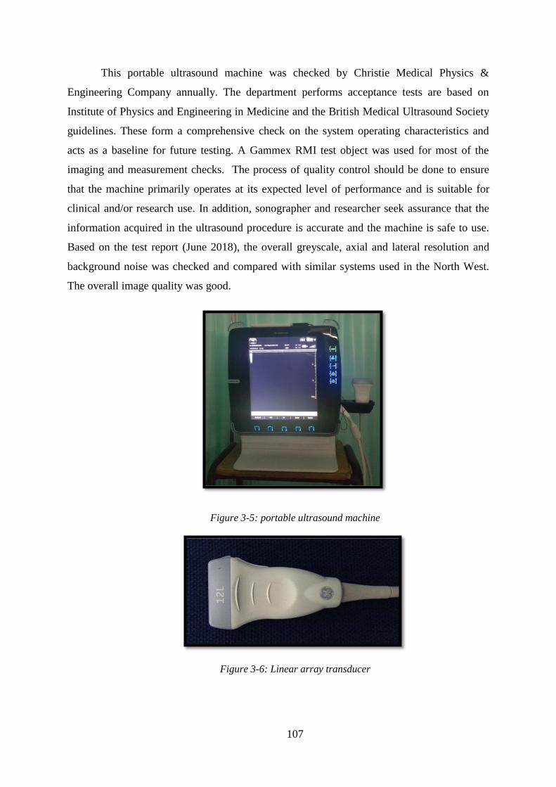
107

This portable ultrasound machine was checked by Christie Medical Physics &

Engineering Company annually. The department performs acceptance tests are based on

Institute of Physics and Engineering in Medicine and the British Medical Ultrasound Society

guidelines. These form a comprehensive check on the system operating characteristics and

acts as a baseline for future testing. A Gammex RMI test object was used for most of the

imaging and measurement checks. The process of quality control should be done to ensure

that the machine primarily operates at its expected level of performance and is suitable for

clinical and/or research use. In addition, sonographer and researcher seek assurance that the

information acquired in the ultrasound procedure is accurate and the machine is safe to use.

Based on the test report (June 2018), the overall greyscale, axial and lateral resolution and

background noise was checked and compared with similar systems used in the North West.

The overall image quality was good.

Figure ‎3-5: portable ultrasound machine

Figure ‎3-6: Linear array transducer

108

3.5.8 Assessment procedure

Once the participants had signed the consent form, they were asked to wear shorts and

take off their shoes and socks in order to leave the lower limbs exposed. The participants

were then asked to sit gently on the examination table in supine position. The researcher

made sure that the participants were comfortable and asked them if they had any questions or

concerns before starting the test. In addition, the researcher locked the testing room to ensure

participants’ privacy and to avoid any distraction. Prior to starting the scanning, the

researcher checked the ultrasound machine and its settings which will be demonstrated in the

next section (3.5.8.1). Once everything was fine, the test started, with the foot is in neutral

position (90 degrees) and then in tension position (the details of the scanning techniques and

measurements will be discussed in the next section). Each structure was imaged in both

longitudinal and transverse scans. The CSA of the structures was measured in transverse

plane. McCreesh and Sinead (2011) reported that no significant difference in the

measurements of the thickness from longitudinal and transverse images and thus either

method could be used. Measuring the thickness on longitudinal image could allow several

areas to be measured on a single image. In addition, longitudinal scanning provides more ease

of transducer alignment on the lower leg (McCreesh & Sinead, 2011). It has been reported in

the literature that measurements of the thickness of tendon should be the same in both

longitudinal and transverse scans. Regardless of the fact that transverse and longitudinal

scanning are both appropriate techniques to measure the thickness of tendon, the longitudinal

plane has some minor advantages. During dynamic scanning, it can be easier to distinguish

between epitenon and the paratenon in the longitudinal plane. Moreover, a longitudinal scan

is an absolute necessity for evaluating the thickness of tendon because it is the only technique

allowing the sonographer to properly record the distance from the bony attachment to the

point where the thickness is measured. Thus, all the measurements are made at the same point

exactly for all participants and measuring the thickness on longitudinal image would be the

method of choice for this study.

The ultrasound images were saved onto a memory card. Once the ultrasound scanning

was completed, the participants had a rest for three to five minutes before starting the second

test (which is described in details in chapter five). Once they had finished both tests, they

changed their shorts and put their socks and shoes back on in the changing room; the

researcher then gave them their vouchers and thanked them for taking part in the study. The

109

researcher was then responsible for cleaning the ultrasound transducer and preparing the

examination bed between participants by applying a new section of paper bed roll.

3.5.8.1 Ultrasound techniques and measurements

The settings for the scanning were as recommended by Liffen (2014) for grey scale

diagnostic ultrasound images to achieve the best resolution and clarity:

- Linear transducer (rectangular shape), most useful for superficial parts and

musculoskeletal (Goyal, 2018), with‎high‎frequency‎≥ 12 MHz.

- Depth adjusted to 3 cm was applicable for the region of interest to be clearly

visualised (Figure 3.7), however it changed sometimes to 4 cm in scanning the

muscles for some participants. Controlling the depth changes the size of the

scanning area. The measurement of the depth appears in most ultrasound

machines to simplify measurement of the size of the structure and the depth of the

field.

- Focus was automatically placed in the middle of the image as a triangular symbol

(Figure 3.7).

- Gain of the image was optimised to adjust overall brightness of the image, which

is in part determined by ambient light in the examination room (Jacobson, 2012).

The gain must be ideally adjusted so that one can recognise the ultrasound

characteristics of normal soft tissue (as described later in chapter four) (Figure

3.7).

- During the scanning, for the Mechanical Index and Thermal Index, the “as low as

reasonably achievable” (ALARS) principle was applied.

110

Figure ‎3-7: An ultrasound image demonstrating the depth scale to the right of the screen

which define by red arrows; Green arrow defines the focus of the image; Blue circle defines the gain

The structures of interest were ATFL, CFL, PBT, PLT, TPT, AT, PBM and PLM.

These were to be scanned in two different foot positions, so that they were measured in a

common position for all and when under tension. Since different structures are orientated

differently and resist different motions, the under tension position varied for different

structures (Table 3.6). The neutral position was performed by asking the participant to sit on

the examination table with their leg fully extended. The examined leg was held in an ankle-

foot orthosis (AFO), with the strap placed around the forefoot, and rested on a sand bag to

maintain the foot in neutral position (0° inversion/eversion and 0° dorsi-/plantar flexion)

(Figure 3.8).

Figure ‎3-8: Right feet hold on AFO for neutral position

111

Table ‎3.6: Summarise the neutral and tension positions for each structure:

Neutral position Tension position

Dorsiflexion Plantarflexion Eversion Inversion

ATFL

CFL

PBT

PLT

TPT

AT

PBM

PLM

To create an ultrasound image, the transducer is held on the skin surface to image the

structures underneath the transducer. An ultrasound gel must be applied to allow the

transmission of the sound beam from and to the transducer by removing the air between the

skin surface and the transducer (more than 99.9% of the sound beam is reflected at a tissue-

air interface, thus no sound beam would be available for imaging) (Goyal, 2018; Jacobson,

2012). The gel used in this study was a thick gel, which is better than a more liquid gel

because it tends to remain localised at the image site. Aquasonic 100 ultrasound transmission

gel has a hypoallergenic, bacteriostatic, non-sensitising, and non-irritating formula. It is the

most widely used gel for diagnostic and therapeutic medical ultrasound (Universal Medical,

2019).

The‎transducer‎must‎be‎grasped‎by‎the‎examiner’s‎dominant‎hand‎between‎the‎thumb‎

and the fingers with the distal part of the transducer close to the ulnar aspect of the hand

(Figure 3.9A). The marker on the transducer must pointed, in a longitudinal scan, towards the

patient’s‎head‎and‎towards‎the‎right‎during‎transverse‎scanning‎(Goyal,‎2018). The transducer

must be stabilised on the skin by either the little finger or the heel of the imaging hand

(Figure 3.9B). This method is necessary to retain appropriate pressure of the transducer on

the skin, to reduce muscle fatigue in the examining arm, to keep the transducer in position

and to avoid involuntary movement of the transducer (Jacobson, 2012).

112

Figure ‎3-9: Transducer held and positioning (Jacobson, 2012).

3.5.8.1.1 Anterior Talofibular Ligament (ATFL)

With the foot in the neutral position, the lateral malleolus was palpated by the

examiner and the proximal edge of the transducer was placed over the anterior border of the

LM bone while distal edge was placed over the talus bone (Figure 3.10).

Figure ‎3-10: Transducer position to scan ATFL

The origin and insertion points of the ATFL were used as bony landmarks; the

anterolateral aspect of LM was identified as the origin of the ATFL while the peak of the

113

talus was identified as the insertion point [similar to previous protocols (Lee et al., 2014;

Sisson, Croy, Saliba, & Hertel, 2011)]. These bony landmarks were clearly identifiable in

ultrasound images due to their hyper-echogenicity (bright white area) and identification of

bony landmarks is also helpful for orientation (Figure 3.11) (Yildizgoren et al., 2017).

Figure ‎3-11: US image for ATFL in neutral position

For the tension position, the AFO was taken off and the participants instructed to

relax the leg muscles while the ankle was passively and manually moved to the end of the

ankle plantar-flexion and inverted range. The sand bags were replaced on the medial and

lateral‎ sides‎ of‎ the‎ participant’s‎ leg.‎ A‎ strap‎ was‎ placed‎ around‎ the‎ lateral‎ forefoot‎ and‎

wrapped around the sand bag to maintain the foot in its plantar-flexed and inverted position

(Figure 3.12). Khawaji and Soames (2015) reported that measurements of ligament lengths

are made for the longest fibres of the ligaments because of the differences in the maximum

range of movement in each position which create differences in ligament length.

Figure ‎3-12: Tension position for ATFL

114

The full length of ATFL was measured from the origin (LM) to the insertion point

(talus) in the longitudinal plane (Figure 3.13A) while the thickness was measured halfway

between LM and talus [as per Dimmick‎et‎al.’s (2009) protocol] (Figure 3.13B).

Figure ‎3-13: Longitudinal measurement of ATFL in tension position. A: The length. B: The thickness

3.5.8.1.2 Calcaneofibular Ligament (CFL)

With the foot in the neutral position, the head of the transducer was placed anterior to

the tip of the lateral malleolus in an oblique coronal plane which positioned the distal part of

the probe towards the heel [as described by De Maeseneer et al. (2009)] (Figure 3.14). This

oblique position is required in order to find the exact location of CFL (De Maeseneer et al.,

2009). The peroneal tendons can help in precisely finding the ligament which is located

proximal to the CFL (Figure 3.15B).

Figure ‎3-14: Transducer position to scan CFL in neutral position

115

For the tension position, a wedge was inserted between the plantar surface of the foot

and the AFO. This helped to dorsiflex the foot (15°) and thus placed the CFL under tension.

The foot was placed on an orthotic insole on the top of the wedge to ensure a smooth foot

contact with the wedge (Figure 3.15A). The measurements of the CFL were taken from

longitudinal plane. The full length of the CFL is rarely visible because the origin underlies

the LM. However, the thickness was measured 1 cm from the insertion point (calcaneus) [as

per the protocol used by Dimmick et al. (2009)] (Figure 3.15B).

Figure ‎3-15: A: Tension position for CFL. B: US measurement for CFL in tension position. PBT:

peroneal brevis tendon, PLT: peroneal longus tendon, and CALC: calcaneus

3.5.8.1.3 Peroneal Tendons

With the foot in the neutral position PLT and PBT were scanned in both longitudinal

and transverse planes. US examination of peroneal tendons commonly starts with transverse

scanning (Taljanovic et al., 2015). For a transverse image, the transducer was placed slightly

inferior to the distal part of the LM in the transverse plane and at the posterolateral ankle (De

Maeseneer et al., 2009) (Figure 3.16A). The peroneus brevis is located near to the LM while

the peroneus longus is seen more superficially (Figure 3.16B) (De Maeseneer et al., 2009).

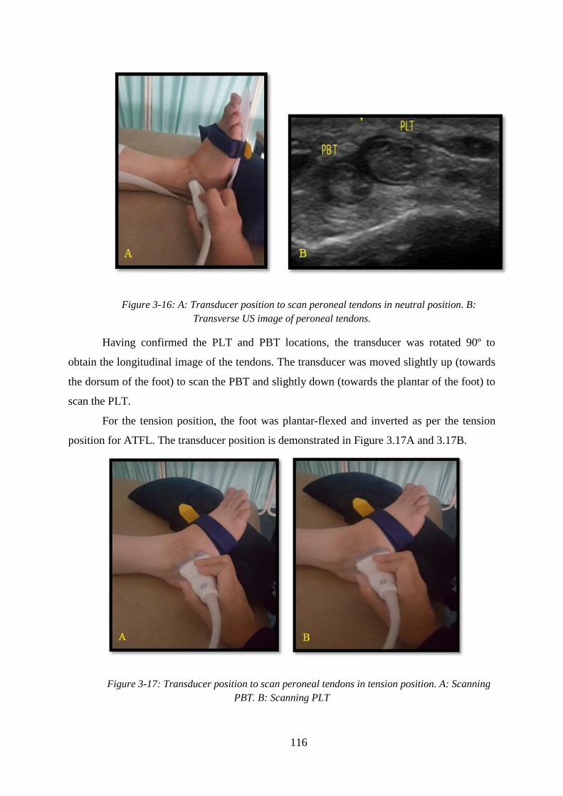
116

Figure ‎3-16: A: Transducer position to scan peroneal tendons in neutral position. B:

Transverse US image of peroneal tendons.

Having confirmed the PLT and PBT locations, the transducer was rotated 90º to

obtain the longitudinal image of the tendons. The transducer was moved slightly up (towards

the dorsum of the foot) to scan the PBT and slightly down (towards the plantar of the foot) to

scan the PLT.

For the tension position, the foot was plantar-flexed and inverted as per the tension

position for ATFL. The transducer position is demonstrated in Figure 3.17A and 3.17B.

Figure ‎3-17: Transducer position to scan peroneal tendons in tension position. A: Scanning

PBT. B: Scanning PLT

117

The measurements of the peroneal tendons were taken 1 cm below LM [as pilot work

has shown that the measurements are the same at the three different locations (at LM, above

LM, below LM)] (Appendix 1). The cross sectional area of the tendons was measured in

transverse plane in the same image for both peroneal tendons (Figure 3.18). However, the

thickness was measured separately for each tendon in the longitudinal plane (Figure 3.19).

Figure ‎3-18: CSA measurement of peroneal tendons

Figure ‎3-19: Thickness measurement of peroneal tendons in tension position. A:PBT

(peroneal brevis tendon). B:PLT (peroneal longus tendon)

3.5.8.1.4 Tibialis Posterior Tendon (TPT)

With the foot in the neutral position, the transducer was placed above the medial

malleolus (MM) in an oblique transverse plane (transverse with an angle) (Figure 3.20A) to

allow a transverse image. The TPT is close to the MM and twice the size of the flexor

digitorum tendon which is located lateral to it (Jacobson, 2012; Lhoste-Trouilloud, 2012).

The transducer was then rotated 90° (Figure 3.20B) to obtain the longitudinal image of the

TPT from which its thickness was measured.

118

Figure ‎3-20: Transducer position to scan the TPT. A: Transverse plane. B: Longitudinal plane

For the tension position, the same procedure as for the ATFL was followed, but with

the foot in a plantar-flexed and everted (rather than inverted) position and the strap on the

medial, not the lateral, side of the forefoot (Figure 3.21A). The measurements of the TPT

were taken 2 cm above the MM. The cross sectional area of the tendon was measured in the

transverse plane while the thickness was measured in the longitudinal plane. An example of

measuring the thickness is demonstrated in Figure 3.21B.

Figure ‎3-21: A: Transducer position to scan longitudinal plane tibialis posterior tendon

(TPT) in tension position. B: Thickness measurement of TPT. MM: Medial malleolus

119

3.5.8.1.5 Achilles Tendon (AT)

The participants were asked to move down the assessment bed to allow the foot to

hang off the end, giving access to the Achilles in neutral position (Figure 3.22A). For the

tension position, the wedge was inserted between the plantar surface of the foot and the AFO

(Figure 3.22B). This kept the foot in a dorsiflexed position. The transducer was placed onto

the palpable Achilles tendon at the posterior ankle in a sagittal plane (Figure 3.22C) to scan

the AT in the longitudinal plane (Figure 3.23A); the transducer was then rotated 90º to obtain

the transverse image of the AT (Figure 3.23B) (Dong & Fessell, 2009).

Figure ‎3-22: Scanning the AT. A: Neutral position. B: Tension position. C: Transducer

position to scan longitudinal plane of AT.

The measurement was taken at the point where the Achilles tendon separates from the

calcanei, which is considered to be the maximum thickness of the tendon (Figure 3.23A)

(Bjordal, Demmink, & Ljunggren, 2003). Furthermore, according to Kharate and Chance-

Larsen (2012), this area is the most common place for tendon pathology with a relative lack

of blood supply (Asplund & Best, 2013). Due to the hypovascularity, this area is more

susceptible to injury. The CSA was measured in the same area (Figure 3.23B).

120

Figure ‎3-23: A: Thickness measurements of AT in longitudinal plane. B: CSA measure of AT

in transverse plane

3.5.8.1.6 Peroneal Muscles

With the foot in the neutral position, the PLM and PBM were scanned in both

longitudinal and transverse planes. For the transverse image, the transducer was placed

perpendicular to the calf bone (fibula), halfway (50%) between the head of the fibula and the

inferior border of the LM (Angin et al., 2014). The transducer was then rotated 90° to scan

the muscles in the longitudinal plane. For the tension position, the position of the leg and foot

was the same as for the tension position of the peroneal tendons (Figures 3.24A – 3.25A).

The measurements of the muscles were taken at the midway point between the head

of the fibula and the inferior border of the LM. The cross sectional area of the muscles was

measured in the transverse plane in the same image (Figure 3.24B), as in the protocol used by

Lobo et al. (2016). The thickness was measured in the longitudinal plane in the same image

(Figure 3.25B).

Figure ‎3-24: A: Transducer position to scan transverse plane peroneal muscles in tension

position. B: CSA measurement of peroneal muscles.

121

Figure ‎3-25: A: Transducer position to scan longitudinal plane peroneal muscles in tension

position. B: Thickness measurement of peroneal muscles.

The ultrasound images were copied to memory drive for later measurement; each

image was coded to a specific number. The computer monitor was a 5 mega-pixel DOME E5

(NDSsi, Santa Rosa, CA,USA; 2048 by 2560 pixels) calibrated to the DICOM Grey Scale

Display Function Standard (The Royal College of Radiologists, 2012). The ambient room

lighting was < 8 lux. The measurements were performed many days later using ImageJ

software, a public-domain, Java-based image processing program developed by the National

Institute of Health (Bethesda, MD). ImageJ software has been shown to have an excellent

inter-rater reliability when measuring the thickness of muscle from ultrasound images

(McCreesh & Sinead, 2011). By the time the measurements were made, the researcher was

blinded to the classification of the groups. The field of view for each ultrasound image was

13.3 x 10.8 cm containing 600 x 655 pixels. A digital caliper was calibrated to 156 pixels per

cm for all images with 3 cm deep and 150 pixels per cm for 4 cm deep images. Data were

imported from ImageJ into an Excel spreadsheet (Microsoft Corporation, Redmond, WA,

USA). All of the data were then analysed with SPSS version 23.00 (SPSS Inc, Chicago, IL,

USA). This method is similar to those used by Croy et al. (2013).

3.6 Image analysis

Length (mm), thickness (mm), and CSA (mm²) of selected ankle structures were

measured using ImageJ software (National Institute for Health, Bethesda, MD, USA) from

ultrasound images, with the researcher (the PhD student) blinded to the participant groups;

the data were then compiled into a Microsoft Excel spreadsheet. The thickness of the

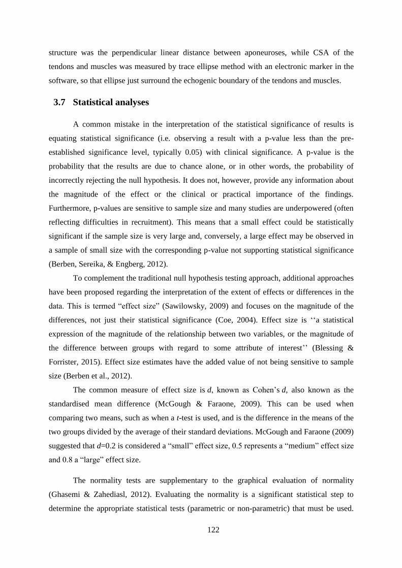
122

structure was the perpendicular linear distance between aponeuroses, while CSA of the

tendons and muscles was measured by trace ellipse method with an electronic marker in the

software, so that ellipse just surround the echogenic boundary of the tendons and muscles.

3.7 Statistical analyses

A common mistake in the interpretation of the statistical significance of results is

equating statistical significance (i.e. observing a result with a p-value less than the pre-

established significance level, typically 0.05) with clinical significance. A p-value is the

probability that the results are due to chance alone, or in other words, the probability of

incorrectly rejecting the null hypothesis. It does not, however, provide any information about

the magnitude of the effect or the clinical or practical importance of the findings.

Furthermore, p-values are sensitive to sample size and many studies are underpowered (often

reflecting difficulties in recruitment). This means that a small effect could be statistically

significant if the sample size is very large and, conversely, a large effect may be observed in

a sample of small size with the corresponding p-value not supporting statistical significance

(Berben, Sereika, & Engberg, 2012).

To complement the traditional null hypothesis testing approach, additional approaches

have been proposed regarding the interpretation of the extent of effects or differences in the

data.‎This‎ is‎ termed‎“effect‎ size”‎ (Sawilowsky, 2009) and focuses on the magnitude of the

differences, not just their statistical significance (Coe, 2004). Effect size is ‘‘a statistical

expression of the magnitude of the relationship between two variables, or the magnitude of

the difference between groups with regard to some attribute of interest’’ (Blessing &

Forrister, 2015). Effect size estimates have the added value of not being sensitive to sample

size (Berben et al., 2012).

The common measure of effect size is d,‎ known‎ as‎ Cohen’s d, also known as the

standardised mean difference (McGough & Faraone, 2009). This can be used when

comparing two means, such as when a t-test is used, and is the difference in the means of the

two groups divided by the average of their standard deviations. McGough and Faraone (2009)

suggested that d=0.2 is considered a “small”‎effect‎size,‎0.5‎represents‎a‎“medium”‎effect‎size‎

and‎0.8‎a‎“large” effect size.

The normality tests are supplementary to the graphical evaluation of normality

(Ghasemi & Zahediasl, 2012). Evaluating the normality is a significant statistical step to

determine the appropriate statistical tests (parametric or non-parametric) that must be used.

123

The Kolmogorov-Smirnov (K-S) test seems to be the most common test for normality.

However, researchers have proposed that this test should no longer be applied because of its

low power (Ghasemi & Zahediasl, 2012). It is highly recommended to use the Shapiro-Wilk

test to assess normality in addition to visual evaluation (Ghasemi & Zahediasl, 2012; Thode,

2002).

Since the data was normally distributed, a series of one-way analyses of variance

(ANOVA) tests were performed to investigate significant differences in demographics,

length, thickness and CSA for the selected ankle structures between groups (healthy vs coper

vs CAI), as well as for the different foot positions (neutral and tension) between the three

groups. Post-hoc Bonferroni tests were performed to provide pairwise comparisons with an a

priori alpha level set at p < 0.05.‎Cohen’s‎d effect sizes were calculated, with d = 0.20 - 0.49

considered as‎a‎‘small’ effect size, 0.50 - 0.79 as‎‘medium’‎and‎˃‎0.80‎as‎‘large’.

According to Kent State University (2019), dependent t-test compares two means that

are from the same individual. Thus, dependent sample t-tests were done to evaluate for

significant differences between right and left limbs. On the other hand, independent sample t-

tests were used to evaluate the significant differences between male and female, and between

normal weight and overweight participants. The difference between equivalent measures was

considered to be statistically significant if the corresponding p value was less than 0.05. Data

analyses were performed using SPSS software version 23.0.

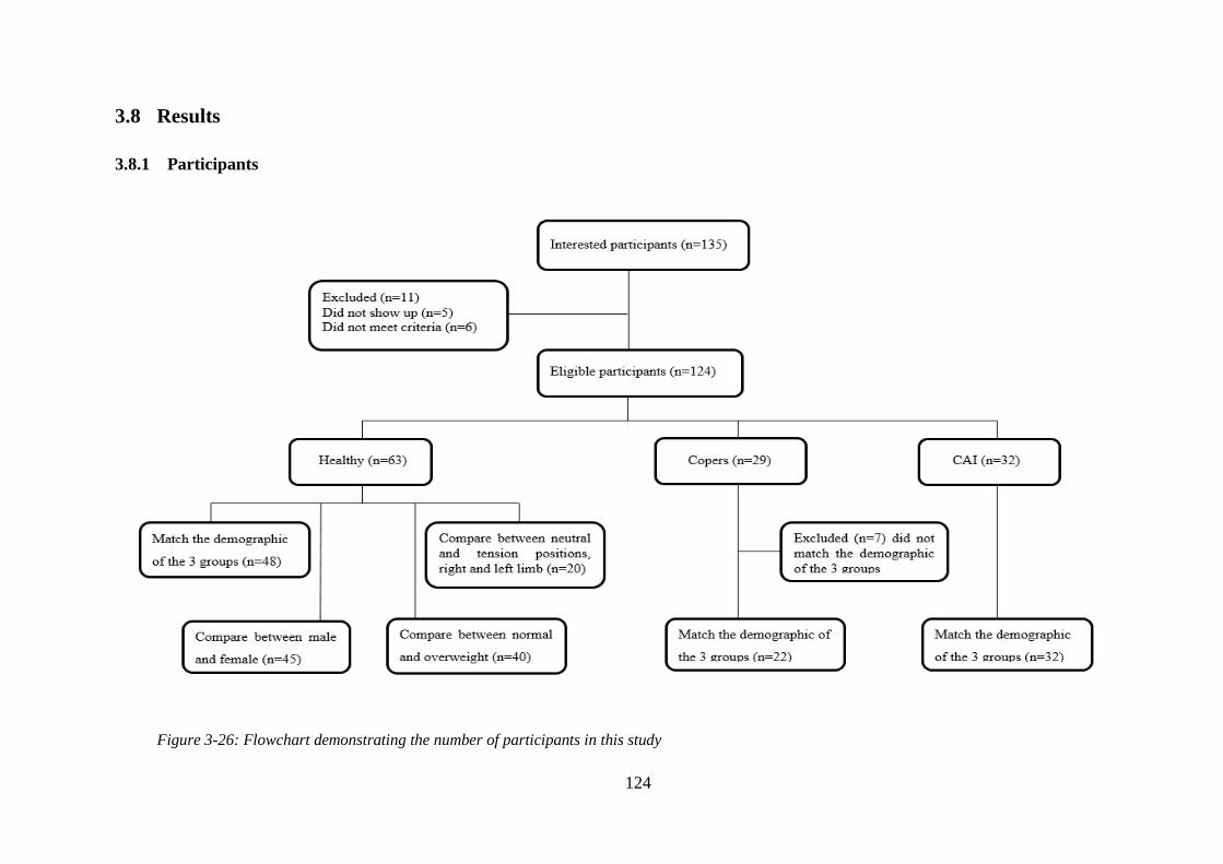
124

3.8 Results

3.8.1 Participants

Figure ‎3-26: Flowchart demonstrating the number of participants in this study

125

3.8.2 Comparison of length, thickness and CSA of selected ankle structures between

healthy, coper and CAI

There was no statistically significant difference in the length of ATFL between the

three groups when the ankle was in a neutral position (p=0.57) (Figure 3.27). The ATFL was

a large significantly longer when under tension in CAI (23.61 ± 1.10 mm) and coper (23.48 ±

0.82) compared to healthy participants (22.22 ± 1.47 mm) (Figure 3.27). In other words, a

statistically large significant difference was found with the ankle under tension (p<0.001,

d=1.10) for healthy versus coper participants, and p-value was equal to 0.001 and Cohen’s d

was equal to 1.06 for healthy versus CAI participants, but not for coper versus CAI

participants (p=0.98, d=0.13) (Figure 3.27). The change from neutral length to tension length

in the coper (4.72 mm) and chronically unstable groups (4.79 mm) was greater than that of

the healthy group (3.07 mm).

The ATFL was significantly thicker in copers (2.45 ± 0.38 mm) and CAI (2.93 ± 0.31

mm) compared to healthy participants (1.90 ± 0.16 mm), with p<0.001 and d=1.81, and

p<0.001 and d=4.17 respectively (Figure 3.28). Interestingly, there was a large significant

difference in thickness of ATFL between coper and CAI participants (p<0.001, d=1.40). The

CFL was significantly thicker in CAI (1.82 ± 0.12 mm) compared to healthy participants

(1.68 ± 0.15 mm) (p=0.003, d =1.03) (Figure 3.28). Whilst not statistically significant, the

thickness of CFL had a large effect size when comparing copers to healthy participants

(p=0.87, d=1.03) and copers to CAI participants (p=0.08, d=0.90). There were no meaningful

or significant differences in thickness and CSA of the tendons and muscles between healthy,

coper and CAI participants (p>0.05 and d<0.2) (Figures 3.28 – 3.29). The descriptive

numerical values of length, thickness, and CSA of selected ankle structures between the three

groups are presented in detail in the Appendix 12.

126

Figure ‎3-27: The mean and SD of the length (mm) of ATFL in neutral and tension positions. (N)

Neutral, (T) Tension between the three groups

* CAI is statistically significant longer than healthy participants

§ Coper is statistically significant longer than healthy participants

Figure ‎3-28: The mean and SD of thickness (mm) of selected ankle structures between the three

groups.

* CAI is statistically significant thicker than healthy participants.

§ Coper is statistically significant thicker than healthy participants. ◙

CAI is statistically significant thicker than coper participants.

127

Figure ‎3-29: The mean and SD of the CSA (mm2) of selected ankle structures between healthy, coper


3.8.3 Comparison between neutral and tension position among healthy participants

The descriptive values for selected ankle structures for neutral and tension position

are presented in detail in Appendix 13.

The length of ATFL in two positions (neutral (N) and tension (T)) is represented in

Figure 3.30. The length of ATFL was significantly longer in tension (21.36 mm ± 2.74)

compared to neutral position (18.74 mm ± 1.34).


(N) Neutral, (T) Tension

* ATFL is statistically significant longer in tension position compared to neutral position

0

50

100

150

200

250

300

PLT PBT TPT AT PLM PBM

CS

A (

mm

2)

Structures

mean of healthy mean of coper mean of CAI

0

5

10

15

20

25

30

ATFL (N) ATFL (T)

Len

gth

(m

m)

Structure

mean of neutral position mean of tension position

*

128

The thickness of the measured structures is represented in Figure 3.31. Differences

between neutral and tension positions were not statistically significant for the thickness of the

selected ligaments, tendons, and muscles.

Figure ‎3-31: The mean and SD of the thickness (mm) of selected ankle structures in neutral

and tension positions

The CSA of the measured structures is represented in Figure 3.32. Differences

between neutral and tension positions were not statistically significant for the CSA of the

selected tendons, and muscles.

Figure ‎3-32: The mean and SD of the CSA (mm2) of selected ankle structures in neutral and

tension positions

0

2

4

6

8

10

12

ATFL CFL PL T PB T PT T AC PL M PB M

Th

ick

nes

s (m

m)

Structures


0

50

100

150

200

250

PL T PB T PT T AC PL M PB M

CS

A (

mm

2)

Structures


129

3.8.4 Comparison between right and left limbs among healthy participants

The descriptive values for selected ankle structures for right and left limbs are

presented in detail in Appendix 14.

The length of ATFL in two positions (neutral and tension) and a comparison of the

right (RT) and left (LT) limbs are represented in Figure 3.33. Differences between RT and

LT limbs were not statistically significant for the length of ATFL (Figure 3.33).

Figure ‎3-33: The mean and SD of the length (mm) of ATFL in two positions in RT and LT

limbs

The thickness of the measured structures and comparison of the RT and LT limbs are

represented in Figure 3.34. Differences between RT and LT limbs were not statistically

significant for the thickness of the selected ligaments, tendons and muscles (Figure 3.34).

Figure ‎3-34: The mean and SD of the thickness (mm) of selected ankle structures in RT and

LT limbs

0

5

10

15

20

25

ATFL N ATFL T

Len

gth

(m

m)

Structures

mean of RT limb mean of LT limb

0

2

4

6

8

10

12

ATFL CFL PLT PBT TPT AT PLM PBM

Th

ick

nes

s (m

m)

Structures


130


between RT and LT limbs were not statistically significant or meaningful for the CSA of the

selected tendons and muscles (Figure 3.35).

Figure ‎3-35: The mean and SD of CSA (mm2) of selected ankle structures in RT and LT limbs

3.8.5 Comparison between male and female healthy participants

The descriptive values of selected ankle structures compared between male and

female healthy participants are presented in detail in the Appendix 15.

The length of ATFL in two positions (neutral (N) and tension (T)) and a comparison

the female and male participants are represented in Figure 3.36. Differences between male

and female participants were not statistically significant for the length of ATFL (Figure 3.36).

Figure ‎3-36: The mean and SD of the length (mm) of ATFL in two positions in female and

male healthy participants

0

50

100

150

200

250

300


CS

A (

mm

2)

Structures


0

5

10

15

20

25

ATFL N ATFL T

Len

gth

(m

m)

Structures mean of female mean of male

131

The thickness of the measured structures and a comparison of male and female

participants are represented in Figure 3.37. Differences between male and female participants

were not statistically significant or meaningful for the thickness of the selected ligaments,

tendons and muscles (Figure 3.37).

Figure ‎3-37: The mean and SD of the thickness (mm) of selected ankle structures in female

and male healthy participants


between male and female participants were not statistically significant for the CSA of the

selected tendons and muscles (Figure 3.38).

Figure ‎3-38: The mean and SD of CSA (mm²) of selected ankle structures in female and male


0

2

4

6

8

10

12

ATFL CFL PLT PB T TP AT PL M PB M

Th

ick

nes

s (m

m)

Structures

mean of female mean of male

0

50

100

150

200

250

300


CS

A (

mm

²)

Structures

mean of female mean of male

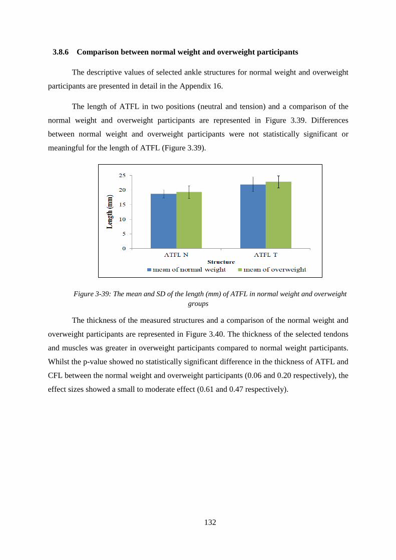
132

3.8.6 Comparison between normal weight and overweight participants

The descriptive values of selected ankle structures for normal weight and overweight

participants are presented in detail in the Appendix 16.

The length of ATFL in two positions (neutral and tension) and a comparison of the

normal weight and overweight participants are represented in Figure 3.39. Differences

between normal weight and overweight participants were not statistically significant or

meaningful for the length of ATFL (Figure 3.39).

Figure ‎3-39: The mean and SD of the length (mm) of ATFL in normal weight and overweight

groups

The thickness of the measured structures and a comparison of the normal weight and

overweight participants are represented in Figure 3.40. The thickness of the selected tendons

and muscles was greater in overweight participants compared to normal weight participants.

Whilst the p-value showed no statistically significant difference in the thickness of ATFL and

CFL between the normal weight and overweight participants (0.06 and 0.20 respectively), the

effect sizes showed a small to moderate effect (0.61 and 0.47 respectively).

133

Figure ‎3-40: Thickness (mm) of the selected ankle structures in normal weight and overweight

participant

* Thickness was statistically significant greater in overweight participants compared to normal

weight participants


between normal weight and overweight participants were statistically large significant for the

CSA of all of the selected tendons and muscles.

Figure ‎3-41: The mean and SD of CSA (mm²) of the selected ankle structures in normal weight and

overweight participants

* CSA was statistically significant greater in overweight participants compared to normal weight

participants

134

3.9 Discussion

3.9.1 Comparison of the length and thickness of the ATFL between healthy, coper

and CAI groups

The main finding of this study is that participants with a history of lateral ankle sprain

had a significantly greater change in the length of their ATFL when the ankle was placed in

tension position, and change in the thickness of the ATFL and CFL compared to healthy

participants. Even though CAI and coper participants showed increased laxity and thickness

of the ATFL, coper participants did not report ankle instability or score low on CAIT.

The ATFL was significantly more elongated at tension position in CAI participants

followed by coper and then healthy participants (23.61 ± 1.79 mm, 23.48 ± 0.82 mm, and

22.22 ± 1.27 mm respectively). While no statistically difference was found in neutral

position (18.82 ± 2.1 mm, 18.76 ± 0.99 mm, and 19.15 ± 1.52 mm). Hypothetically,

lengthening the ATFL leads to reduced constraint on the talus relative to the fibula and tibia,

allowing it to translate anteriorly or rotate medially relative the fibula (Croy et al., 2012). In

other words, stretched or elongated ligaments over a particular point for long period of time

become unable to retain to their original shape. As it happened in our coper and CAI

participants, with the ATFL of CAI participants become more lax and lose their ability to

support the joint properly which could lead to ankle joint instability which demonstrated in

decrease reach distance of the SEBT as shown later in chapter five.

Even though the study demonstrated that ATFL was significantly longer in coper and

CAI compared to healthy group, no significant difference was observed between the coper

and CAI participants. This finding supports Croy et al. (2012) and Liu et al. (2015) who also

found no statistically significant differences in the length of ATFL between coper and CAI

groups. Given‎one‎of‎our‎criteria‎for‎CAI‎group‎was‎a‎feeling‎of‎“giving‎away”, this infers

that changes in the ATFL are not an obvious explanation for these experiences. In addition,

the syndrome of CAI is probably precipitated by a traumatic injury, getting worse by the

dysfunction of sensorimotor and several episodes of ankle sprain reoccurrence. These could

be aggravated by potential undiagnosed cartilage injuries which could be related to

osteoarthritis and poor outcomes (Choi, Lee, & Han, 2008; Valderrabano, Hintermann,

Horisberger, & Fung, 2006).

135

Baezegari and colleagues (2017) reported that the ligament is considered to be thick

when the width is increased more than 2.4 mm or more than 20% of normal lateral ligament.

Several previous studies have compared the thickness of the ATFL in healthy and injured

ankles. The present study measured the thickness of healthy ATFL to be 1.90 ± 0.16 mm

which increased to 2.45 ± 0.38 mm in coper and to 2.93 ± 0.31 mm in CAI. The thickness of

ATFL was found to have increased by approximately 54.21% compared in CAI participants

to healthy participants and increased by almost 29% compared in coper participants to

healthy participants. The thick ligament could be occur due to the scar because of the healing

of the ligament (Cai et al., 2017).

Hua et al. (2008) also reported an increased thickness of the ATFL in acute ankle

sprains, from 1.46 ± 0.21 mm in healthy ankles to 2.71 ± 0.49 mm in injured ankles. An

ultrasound study measured the thickness of the ATFL in healthy and chronic ankle instability

groups (Liu et al., 2015). The authors reported that ATFL was thicker in people with CAI

(2.28 ± 0.53 mm) compared with the healthy group (1.97 ± 0.42 mm). Using MRI rather than

ultrasound, Kijowski and Tuite (2015) deduced that a chronic ankle sprain leads to a

thickening of the ligament without surrounding haemorrhage and edema.

Contrary to the results of Dimmick et al. (2009), whose MRI-based data study

indicated there was no statistically significant difference in the thickness of the ATFL

between normal and injured participants. In men, the mean thicknesses of healthy and

previously injured ATFLs were 2.44 ± 0.49 mm and 2.26 ± 0.53 mm respectively, and 2.16 ±

0.47 mm and 2.18 ± 0.61 mm respectively for females. It is possible that these results were

due to the very small sample size used in the study (male: ten healthy and nine injured,

female: nine healthy and five injured). Moreover, there was no information regarding the type

of ankle injury, whether it was acute or chronic, or how long it had been since the participants

were injured.

Whilst not statistically significant, the ATFL in the present study was almost 20%

thicker in the CAI group compared to copers. This contrasts with Liu et al. who found no

such difference, although they only reported a 15% greater thickness in CAI compared to

healthy participants, and the equivalent figure in this work is 54.21%. The critical difference

between Liu et al.‎ and‎ this‎work‎ is‎ that‎ in‎ Liu’s‎ CAI‎ participants‎were‎ selected‎ based‎ on‎

CAIT‎ score‎ regardless‎ the‎ number‎ of‎ previous‎ ankle‎ sprains‎ and‎ the‎ sensation‎ of‎ “giving‎

away”.‎This‎is‎contrary‎to‎recent‎definitions‎of‎CAI‎(Gribble‎et‎al.,‎2014).‎In‎contrast‎we‎did

136

not differentiate participants exclusively by CAIT scores, but used the number of prior

sprains‎and‎the‎sensation‎of‎“giving‎away”‎to‎differentiate‎CAI‎and‎copers.‎

In order to decrease 70% of the reoccurrence of ankle sprain, it is important to fully

understand the reason that prevents coper people from having another sprain (Liu et al.,

2015). The finding of our study showed that the morphologies of the coper are different from

healthy ankles. This is contrary to previous studies which have suggested that morphologies

of the coper are similar to healthy ankles. They concluded that structure of the ligament is not

the only caused for ankle instability.

3.9.2 Comparison of the thickness of CFL between healthy, coper and CAI groups

The CFL is often involved in ankle ligament sprains and chronic lateral instability

(Kitsoulis et al., 2011). In other words, the CFL affected in 50 - 75 % of cases of ankle sprain

(Apoorva et al., 2014). Thus, a good knowledge and understanding of ankle anatomy is

essential for diagnosis injuries. In the current study, the mean thickness of CFL for healthy

participants was 1.68 ± 0.13 mm, which matches results from earlier cadaveric studies by

Apoorva et al. (2014) and Kitsoulis et al. (2011) (1.64 ± 0.43 mm and 1.60 mm respectively).

The result of our study showed increased CFL thickness by 8.3% in CAI participants

compared to healthy participants. This is in line with Hua et al. (2008) who used MRI and CT

to report thickness increased in acute ankle sprain. Whilst not statistically significant the

thickness of CFL had a large effect size when comparing copers to healthy (p =0.87, d =1.03)

and copers to CAI (p = 0.08, d = 0.90). To the best of our knowledge this is the first study to

measure the CFL in healthy, coper and CAI groups by using musculoskeletal ultrasound.

3.9.3 Comparison of the thickness and CSA of selected ankle structures between

healthy, coper and CAI groups

It has been reported that inversion ankle sprain may not only damage the ATFL and

CFL, but it may also disturb the peroneal tendons (Park et al., 2010). However, the data in

this present study does not support this, with no statistically significant change observed in

the thickness and CSA of peroneal tendons between healthy, coper and CAI participants.

The thicknesses of healthy peroneal longus and brevis muscles are in line with those

of previous studies. Angin et al. (2014) reported the average thickness of peroneal muscles as

13.0 ± 1.8 mm and Crofts et al. (2014) measured the thickness of peroneal muscles as 13.5 ±

1.9 mm. However, these two studies measured the full thickness of peroneal muscles without

137

separating PLM from PBM. Furthermore, the results of the present study did not reveal any

significant change in the thicknesses of peroneal muscles between the three groups. This is

the first data to demonstrate the thickness of peroneal muscles separately in healthy, coper

and CAI groups.

In addition to measuring the thicknesses of the peroneal muscles, the present study

measured the CSA of the peroneal muscles; PLM values in healthy ankles (73.9 ± 4.2 mm²),

in coper (74.0 ± 4.1 mm2), and in CAI (74.5 ± 5.2 mm²). However, Lobo et al. (2016)

reported that the CSA of PLM in healthy ankles was 50 ± 20 mm² and in LAS was 40 ± 20

mm². On the other hand, CSA of PBM in the current study was 234.7 ± 31.7 mm² for healthy,

246.2 ± 28.1 mm2 for coper, and 256.4 ± 31.5 mm² for CAI ankles. A previous study

demonstrated that CSA of PBM in healthy ankles was 350 ± 70 mm² and in LAS was 320 ±

70 mm² (Lobo et al., 2016). Furthermore, Angin et al. (2014) and Crofts et al. (2014) reported

the CSA of peroneal muscles for healthy ankles to be 382 ± 63.0 mm² and 409 ± 125.0 mm²

respectively. However, they do not separate the PLM from PBM during the measurement.

The findings of the current study demonstrated that the CSA of peroneal muscles in coper

and CAI groups does not differ from that of healthy group. However, this finding does not

support the previous research, which demonstrated that the CSA of the peroneus longus

muscle is reduced in LAS participants compared to healthy ones. The age of control and

injured‎ participants‎ in‎ Lobo’s‎ study‎were‎ statistically‎ significantly‎ different‎ (p <0.05) and

Kim, Ko, Lee, Ha, & Lee, (2015) and Fujiwara et al. (2010) found that the thickness and

CSA of lower extremity muscles changes with age. The reasons why PLM are the only

muscles to be changed with LAS in‎Lobo’s‎study‎were unclear. Moreover, the differences in

the measurement of peroneal muscles between the studies could be due to the differences in

inclusion criteria for the groups, differences in the techniques or the traces that are used to

outline the boundary of muscles.

Since unrecognised acute Achilles tendon has been reported in severe ankle sprain

(Lam & Lui, 2015), and it has been reported that 12.2% of ankle sprain cases involved

Achilles tendinitis (Fallat et al., 1998), it was important to include Achilles tendon in this

study to have a baseline knowledge for accurate diagnosis. The results from the present study

demonstrates that the thickness and CSA of AT in healthy was 4.01 ± 0.61 mm and 51.0 ±

4.5 mm2, in coper was 4.03 ± 0.53 mm and 51.40 ± 2.90 mm

2, and in CAI was 4.01 ± 0.62

mm and 51.90 ± 3.80 mm2 respectively which reveal no statistically significant differences

being found between the three groups. Daftary & Adler (2009) stated that the thickness of a

138

normal AT should not exceed 6 mm, based on their ultrasound study. Hodgson et al. (2012)

evaluated the thickness of AT in patients with spondyloarthritis and a healthy control group

using MRI and ultrasound imaging. They reported that the close to the data obtained from

previous studies. Ying et al. (2003) found that the CSA of AT at the level of the medial

malleolus was 56.91 ± 7.58 mm², and Yildiz and Turksoy (2007) reported the CSA as 60.78

± 13.09 mm² (based on 80 ankles). A possible explanation of the smaller value in the present

study may be due to the differences in calliper settings. The present study does not include

the paratenon (superficial areolar connective tissues upon which the AT rests) (Shapiro,

2015) of the tendon during the measurements.

Results of this study showed that there were no statistically significant differences in

the thickness and CSA of TPT between the three groups. The present study followed Neville

et‎al’s (2010) protocol, according to which the thickness was measured at approximately 2

cm proximal to the tip of the medial malleolus, and finding the thickness of TPT to be 2.9

mm, while in this study it was measured as 2.50 ± 0.17 mm. However, Perry et al. (2002)

measured the thickness of TPT using longitudinal ultrasound images at around 1 cm distal to

the end of the medial malleolus and found the thickness to be 3.0 ± 0.7 mm. The results of

these studies are consistent despite that the authors taking measurements from different

locations.

The researcher used CSA and the thickness as surrogates of the force passing through

the structures and their functional role. Increased thickness and CSA could reflect increased

mechanical loading on tendons due to increases in muscle strength or use (Taş‎et‎al.,‎2017).

In the face of evidence for no differences in muscle or tendon structures, the efficiency of

motor control strategies during inversion incidents is perhaps a more likely explanation for

differences between copers and CAI.

Knowing the CAI is a complicated issue, it is essential to acquire a comprehensive

understanding of all the possibility changes that occurred to an individual to realise the

differences between who experience several ankle sprains and those who are classify as ankle

copers (Liu et al., 2015).

3.9.4 Comparison of selected ankle structures between neutral and tension position

It has been stated that an increase in the ATFL length beyond 20%, equivalent to 4

mm, is enough to cause ligament failure and joint instability (Croy et al., 2012; Jeys, 2004).

No previous studies involving healthy ankles have observed 20% ATFL lengthening.

139

However, in this current study, the length of the ATFL in CAI participants increased by 4.79

mm between the neutral (18.82 mm) and the tension (23.61 mm) positions, a change of

approximately 25.45%. This is in line with Croy et al. (2012) who used stress

ultrasonography during inversion and anterior drawer tests. They found that the length of the

ATFL in CAI participants increased by 4.7 mm from the neutral (18.8 mm) to the inversion

positions (23.5 mm), a change of 25%. However, the length in healthy participants did not

exceed 15% from neutral (19.15 mm) to tension (22.22 mm) positions. This illustrates the

importance of studying ligament competency under loaded conditions and not simply passive

ligament morphology. Increases were circa 16% in our healthy group, 25.2% in the coper

group, and 25.45 % in the CAI group.

These findings compare favourably with the finding of de Asla et al. (2009), who

measured the change in the ATFL healthy male participants when the foot was moved from a

neutral position (16.3 ± 3.00 mm) to a maximal plantarflexion (20.8 ± 2.7 mm) using a

combined dual-orthogonal fluoroscopic and MRI techniques. Khawaji and Soames (2015)

also measured the changes in ATFL length in their sample of 50 cadaveric feet. They

reported that the length of the ATFL changed from 20.17 ± 3.4 mm to 21.06 ± 06 mm during

plantar flexion from a neutral position, in a study using electronic digital Vernier callipers.

When the foot is positioned in the plantar flexion position, the alignment of the ATFL

fibres adapts to this position and most likely plays the role of the main collateral ligament in

constraining further movement. Because most lateral ankle sprains happen during plantar

flexion, the ATFL would therefore be the initial lateral collateral ligament to be affected and

damaged (de Asla et al., 2009). This concept has been corroborated by several in-vitro studies

which have investigated strain in the ATFL in response to loading in different foot positions.

Renstrom et al. (1988) found that the strain of ATFL increased by 3.3% when the ankle joint

moved from 10° of dorsiflexion to 40° of plantarflexion. Stephenson, Charlton & Thordarson

(2012) found that strain on the ATFL increased as the ankle moves from 20° of dorsiflexion

to 30° of plantar flexion. The highest rate of increase occurred between the neutral position

and 20° of plantar flexion (Colville et al., 1990). Colville et al. (1990) evaluated the strain in

lateral ankle ligaments using implanted strain gauges, by moving the foot through inversion,

eversion, and internal and external rotation whilst flexing, along with on-extension arc of

motion in ten cadaveric ankles. They found that the greatest rate of increased ATFL strain

occurred when the foot changed position from neutral to 20° of plantar flexion. Moreover,

Ozeki et al. (2002) studied strain in the central fibres of the ATFL in 12 cadaveric ankles in

140

plantar flexed and dorsal flexed positions. Strain was found to increase as the ankle was

plantar flexed, inverted and internally rotated. This helps to explain why the ATFL is the

ligament affected in all cases of inversion ankle sprains, since it is the most important for

movement restraint and yet also the weakest (Attarian, McCrackin, Devito, McElhaney, &

Garrett, 1985; Jeys, 2004). These studies proposed that the ATFL would tighten in plantar

flexion. Thus, excessive and explosive plantar flexion when the ankle joint is inverted could

produce stress and may rupture the ATFL (Fong et al., 2012b).

The viscoelastic properties of the ATFL along with the crimped arrangement of

collagen fibres, influence the mechanical behaviour of the ATFL under load (Hauser et al.,

2013). The relationship between the mechanical properties of the ligaments and changes in

the crimp pattern is expressed in terms of their stress-strain relationship. The four regions of

the stress-strain curve are illustrated in Figure 3.42.

Figure ‎3-42: Four regions of the stress-strain curve (Korhonen & Saarakkala, 2011)

When the foot is in a neutral position, the ATFL is largely unstressed and the collagen

fibres bind with elastic and reticular fibres to create the sinusoidal pattern referred to as the

“crimp”‎pattern‎(Raut & Mate, 2016). This pattern is demonstrated by the first region of the

stress-strain curve, or the toe region. When force is initially applied to the tissue it is

transferred to collagen fibrils, causing the fibrils to laterally shrink, water to be released, and

the crimp of the ligament to be progressively lost as the ligament is elongated, until all fibres

are almost straight. This second region of stress-strain curve is called the elastic (linear)

region (Raut & Mate, 2016). As the ligament is exposed to more strain, the microstructure of

the ligament is disrupted and partially tears (third, or plastic region). Further elongation

causes a complete rupture of the ligament (failure region) (Raut & Mate, 2016).

141

A computational biomechanics study has been done to study the effect of different

combination of joint movement on the strain of different ankle ligaments (Fong et al., 2011).

The authors found that the highest strain was seen in the ATFL with combination of plantar

flexion, inversion, and internal rotation (Fong et al., 2011) which could be the most probably

the mechanism of the ankle sprain injury for our participants since ATFL was the most

affected ligament compared to CFL.

Whilst this study demonstrated no statistically significant differences in the thickness

and CSA of the provided ankle structures between the neutral and tension positions, it is

important for the sonographer to know the appearance of each structure in different ankle

joint positions in order to provide an adequate patient position which plays a significant role

in providing an appropriate ultrasound image. In addition, knowing that there was no

difference between the neutral and tension positions. Neutral position was considered to be

the optimal position for ultrasound imaging of the selected ankle structures (PBT, PLT, TPT,

AT, PBM, and PLM) without‎placing‎the‎participant’s‎feet‎into‎tension‎position,‎making the

scan easier for both participants and sonographer.

3.9.5 Comparison between right and left limbs of healthy participants

The present study evaluates the length, thickness and CSA of selected ankle structures

in 20 healthy ankles to find the degree of symmetry between the right and left limbs. The

present study found that the length of the ATFL and thickness of the ATFL and CFL were the

same for the right and left ankles. This finding supports Khawaji and Soames (2015), who

showed that the length of the ATFL did not differ between left and right ankle in males and

females, and Liu et al. (2015), who also found no differences between right and left in

healthy ankles. In addition, the mean CFL thickness was found to be similar between right

and left healthy ankles (Apoorva et al., 2014).

No significant variation in the thickness and CSA of the tendons and muscles was

found. This result is in line with those of previous studies. Bjordal et al. (2003) concluded

that the differences in Achilles tendon thickness between the two sides were very small and a

difference of only 0.8 mm could be established for healthy tendons. Andrade et al. (2006)

reported that the thickness of Achilles tendons between right and left in 100 healthy ankles

was similar. Furthermore, Ying et al. (2003) found that the thickness of Achilles tendons in

the dominant and non-dominant ankles was similar in both the frequent exercise group (> 6

hours every week) and the infrequent exercise group (< 1 hour every week). It has been

142

reported previously that there was a significant difference in the thickness of leg muscles

between dominant and non-dominant legs of junior soccer players because of the preferential

use of one limb over another (Kearns, Isokawa, & Abe, 2001). This is consistent with

previous research on Gaelic footballers which found a similar dominance effect in the

anterior tibial muscles with the dominant side being 7.3% thicker. These differences were not

seen in non-football players and thus the difference observed in footballers could be related to

sport-specific performance (McCreesh & Sinead, 2011). Sonographers may take this

difference into consideration when scanning sports players to evaluate the dimensions of their

muscles.

It was important for the researcher to compare the length, thickness and CSA of

selected ankle structures between the right and left limbs to have a complete characterisation

of healthy ankles and to know if it is necessary for the researcher to scan either healthy limbs

or just one of them for comparison with injured limb.

3.9.6 Comparison between female and male healthy participants

To gain greater insight into sex-based differences in selected ligaments, tendons and

muscles, the researcher assessed the length, thickness, and CSA of selected ankle structures

from healthy male and female using ultrasound scanning. This ultrasonographic study found

that although the ultrasound measurements of the thickness, CSA and the length selected

ankle structures (ATFL, CFL, PBT, PLT, TPT, AT, PBM, and PLM) were greater in males

with the same BMI, this was not statistically significant. Sarver et al. (2017) recently

evaluated the gender differences in tendon structure and function in an in-vitro study. Authors

reported that there was a great level of similarity in the morphology and behaviour of tendon

between male and female mice. They concluded that, even though there was some variance in

the size, cellular composition, transcriptome (i.e. the total set of Ribonucleic acid (RNA)

species in a tissue), and proteome (i.e. the total set of proteins in a given tissue) (Passos,

2015), the gender variances in the structure and function of tendon were small (Sarver et al.,

2017).

In contrast, Khawaji and Soames (2015) reported significant differences in the length

of the ATFL between males and females, and Chow et al. (2000) found that the average

muscle thickness was greater in males compared to females. The number and size of muscle

fibres play an important role in muscle characterisation (Cheuvront, Moffatt, & DeRuisseau,

2016). While some studies have concluded that males have a greater number of muscle fibres

143

(Meth, 2001), others have shown males to have the same number as females (Cheuvront et

al., 2016). Moreover, authors demonstrated that increased the thickness of the muscles is a

result of increase the diameter of a muscle fibre with constant fibre number and length, and

muscle length (Maxwell, Faulkner, & Hyatt, 1974). However, Kubo et al. (2003) found that

fascicle length of gastrocnemius muscles was similar between male and female. While Chow

et al. (2000) demonstrated that female had longer fascicle length of the triceps surae muscles

than male. These contradictory results may be due to variations in the methodology and

sampling used, and it is difficult to determine if the number of muscle fibres is actually

different between genders. Another possible explanation is the changing sizes of muscle

fibres. Muscle fibres have different diameters, from 10 to 100 µ (Mair & Tome, 2013) with

Cheuvront et al. (2016) and Meth (2001) having deduced that the individual muscle fibres in

females are smaller than those in males.

3.9.7 Comparison between normal weight and overweight healthy participants

The present study was also designed to determine the effect of BMI on the length,

thickness and CSA of selected ankle structures. BMI is the metric that is now utilised to

define adult anthropometric weight/height characteristics and to categorise them into different

groups (Nuttall, 2015). The results of this study highlight a significant aspect for

consideration in the measurement of selected ankle structures. The thicknesses and CSA of

the selected ankle structures (PLT, PBT, AT, TPT, PLM, and PBM) were found to be

statistically significant thicker among overweight participants compared to those with normal

BMI with p-value less than 0.05. Whilst the p-value showed no significant differences in the

thickness‎of‎ ankle’s ligaments, overweight participants had thicker ligaments with small to

medium effect size (Cohen’s‎d = 0.47 - 0.61 for CFL and ATFL respectively). The results of

the present study agree with Abate (2014) and Klein et al. (2013), who deduced that a higher

BMI can lead to increased AT thickness. The most significant reason behind increased

thickness of the tendon could be due to increased mechanical loadings on the tendon because

of increased body weight and the increased strength of the muscle (Taş‎ et‎ al.,‎ 2017).

Mechanical loading is necessary for tendon homeostasis to continue. If the mechanical

loading continues increasing, anabolism becomes dominant over catabolism, and the

thickness and CSA of the tendon increase through the generation of new extracellular matrix

and collagen fibres (Abate et al., 2009; Kubo et al. 2003).‎Taş‎et‎al.‎(2017)‎mentioned‎that the

thickness of the tendon increases as a compensatory mechanism to reduce increased

144

mechanical loadings on the tendon and avoid deformation of the tendon due to increased

body mass and/or muscle strength.

A number of studies have tested the association between BMI and the size of some

ankle structures (Abate, 2014; Klein et al., 2013). Mirza (2016) proposed that BMI is a factor

that engaged in altering the physical form of Achilles tendon by changing its thickness. The

author concluded from his ultrasound study that the thickness of the AT is BMI-dependent, as

overweight participants have a thinner Achilles tendon. In other words, thickness of Achilles

tendon decreases as the BMI increases. This, however, contradicts the findings of the current

study, where Achilles thickness was found to be greater in those who were overweight. The

classification of overweight participants differs‎ between‎ the‎ two‎ studies,‎ with‎ Mirza’s‎

overweight category overlapping with the obese in the current study. In addition, Mirza

included a very small sample size (5 participants in each group).

3.10 Limitation

The researcher acknowledges some limitations to this study. Ultrasound is considered

to be an operator-dependent. It needs a training course to master its scanning techniques.

Based on the previous studies, agreement between senior sonographer with 10 years

experiences and the beginner sonographer improved within two months (Backhaus et al.,

2010). Gun et al. (2013) reported that after a six hour training program to a strict protocol,

emergency physicians could utilise bedside ultrasonography to assess patients with suspected

ATFL injury. Therefore, they suggested that a relatively short period of training has the

ability to allow sonographers to provide adequate US imaging (Backhaus et al., 2010). In

addition, the researcher did not classify if injured participants had combined ligament injures

to ATFL and CFL, and it could be that these kind of injuries have impact on the results.

Despite the limitation, the present study provides novel insight into the structural features of

selected ankle structures in healthy, coper and CAI groups.

3.11 Conclusion

Foot and ankle injuries may affect the body function. Therefore, the early diagnosis and

particularly designed treatment will improve the prognosis. Ultrasound scanning has been an

imaging modality to study muscular tissue for many years. This study characterised and

compared selected ankle structures by using ultrasound in participants with and without a

history of previous ankle sprain. The findings of study indicate that the ultrasonography is a

145

reliable and effective method that can be utilised to detect participants’‎ ankle ligamentous

injury.

Among the selected ankle structures, the length of the ATFL and the thickness of the

ATFL and CFL were the only ones which showed statistically longer and thicker in injured

groups (coper and CAI) compared to healthy participants. ATFL was longer and thicker in

both coper and CAI participants and thicker but not longer in CAI compared to coper

participants. For the healthy group, no statistically significant differences were found in the

length, thickness, and CSA of the selected ankle structures between the right and left limb,

nor females and males. However, the thickness and CSA of most of the selected ankle tendon

and muscles was larger in overweight compared to normal weight healthy participants.

Knowledge the characterisation of normal and injured ligaments, tendons, and muscles

is important for diagnosing the ankle sprains. Moreover, it is important for planning

rehabilitation programmes for patients with ankle sprains, as changing in ligament size has

been reported in injured participants. Structural changing of the ankle ligaments opens new

horizons to investigate if the thickness of the ankle ligaments is related to functional deficits

in injured ankles which lead the researcher to conduct a functional study (chapter five). On

the basis that no differences were found in the selected muscles and tendons structures we

measured, motor control strategies might be a more likely explanation for differences

between coper and CAI cases.

146

4 Chapter four: Quantitative evaluation of ultrasound images to

compare healthy and injured anterior talofibular ligaments


A digital ultrasound image is a two-dimensional numerical matrix (Diaz et al., 2015)

that reflects signal echoes that have experienced different attenuation (less or high) after

passing through various tissue. Digital images are created from a large number of elements

named pixels and a pixel has a numerical value and is the fundamental quantify the

ultrasound signal (Diaz et al., 2015). Each pixel is represented by grey-level (brightness)

intensity, which helps radiologists and sonographers to interpret the structure together with

the related anatomical and clinical information (Diaz et al., 2015).

According to Tamborrini (2014), musculoskeletal structures have various

echogenicities and different reflection ratios which define their ultrasound appearance.

Changes in echogenicity of an injured ligament and tendon are one of the most significant

criteria in the use of musculoskeletal ultrasound images (Agut et al., 2009). What we know

about the normal sonographic appearance of tendons and ligaments is largely based on

subjective evaluations of their echogenicity. The echogenicity of an injured ATFL is ‘darker’

than the healthy equivalent, but the degree of difference in echogenicity is unknown. Work in

this chapter sought to quantify echogenicity in the ATFL, focusing on this structure because

chapter three revealed it to be the most structure differing between healthy, coper, and CAI

groups. The assumption made in this study was that quantitative analysis of the echogenicity

may offer further insights into the nature and scale of changes in the ligaments post-injury.

This study, which is the first of its kind to deal with the ATFL ultrasound images, will

benefit and use the information provided by healthcare providers to distinguish of the ATFL

between healthy, coper and CAI participants. The quantitative analysis was performed by

ImageJ as traditional method in the literature.

4.2 Aims, objectives, and hypothesis of the study

Since the length and the thickness of the ATFL were the only structures different in

the injured groups (coper and CAI) compared to healthy participants from the previous study,

this study aimed to provide a quantitative analysis of echogenicity of the ATFL. Providing a

147

numerical and objective estimate of echogenicity could enhance our understanding of the

structural changes that might have occurred in previously sprained ankles. To achieve this

aim, the following objectives were established:

- Evaluate the echo intensity value of the ATFL in healthy, coper and CAI

participants by using computer-aided greyscale analysis.

- Evaluate the differences in ATFL echo intensity between the three groups.

Hypothesis: There will be statistically significant differences in the echo intensity value of

the ATFL between healthy, coper, and CAI participants.

4.3 Methods

4.3.1 Image dataset

Ultrasound images of the ATFL were obtained using a linear array transducer (12.7

mm x 47.1 mm) with 5-13 MHz of a portable Venue 40 musculoskeletal ultrasound system

(GE Healthcare, UK). Data were collected from 60 participants (20 healthy, 20 coper, and 20

CAI) with mean age 28.13 ± 7.33 years and mean BMI 24.47 ± 2.51 kg/m2. The size of the

ultrasound images was 600 x 655 pixels with 256 grey-levels. Ultrasound machine settings

(gain and probe frequency) were constant to ensure that the value of greyscale pixel was the

same (described in 3.5.8.1). The ultrasound protocol used to scan the ATFL was described

previously in section 3.5.8.1.1.

4.3.2 Quantification echogenicity of ATFL

Echo intensity can be measured by taking the average of the greyscale value of every

pixel in a particular “region of interest”‎ (ROI) on an ultrasound image (Varanoske et al.,

2016). Differences in shades of grey are used to discriminate different kinds of tissue, analyse

relationships between the structures, and may reflect physiological function (Balakrishnan,

2014). The mean echo intensity of the ATFL was determined using a computer-aided

greyscale analysis of the echo signals in regions of interest.

Longitudinal images of the ATFL were taken as per the previous study (chapter three)

in JPEG (Joint Photographic Experts Group) format. However, the images were displayed on

a computer monitor which is 5 mega-pixel DOME E5 (NDSsi, Santa Rosa, CA, USA; 2048

by 2560 pixels) calibrated to the DICOM Grey Scale Display Function Standard. All

ultrasound images were analysed offline through the standard histogram function in image

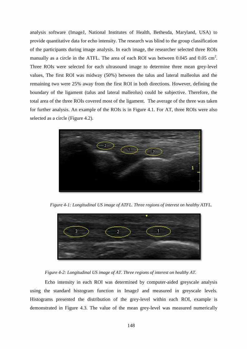
148

analysis software (ImageJ, National Institutes of Health, Bethesda, Maryland, USA) to

provide quantitative data for echo intensity. The research was blind to the group classification

of the participants during image analysis. In each image, the researcher selected three ROIs

manually as a circle in the ATFL. The area of each ROI was between 0.045 and 0.05 cm2.

Three ROIs were selected for each ultrasound image to determine three mean grey-level

values, The first ROI was midway (50%) between the talus and lateral malleolus and the

remaining two were 25% away from the first ROI in both directions. However, defining the

boundary of the ligament (talus and lateral malleolus) could be subjective. Therefore, the

total area of the three ROIs covered most of the ligament. The average of the three was taken

for further analysis. An example of the ROIs is in Figure 4.1. For AT, three ROIs were also

selected as a circle (Figure 4.2).

Figure ‎4-1: Longitudinal US image of ATFL. Three regions of interest on healthy ATFL.

Figure ‎4-2: Longitudinal US image of AT. Three regions of interest on healthy AT.

Echo intensity in each ROI was determined by computer-aided greyscale analysis

using the standard histogram function in ImageJ and measured in greyscale levels.

Histograms presented the distribution of the grey-level within each ROI, example is

demonstrated in Figure 4.3. The value of the mean grey-level was measured numerically

149

based on the 256 degrees of greyscale labelled by the software, from 0 (black) to 255 (white),

for each pixel within the ROI. The mean grey-level of the three ROIs values was calculated

as the final grey scale value for each image.

Figure ‎4-3: Histogram analysis shows the distribution of the intensity of ATFL tissue. The

vertical axis demonstrates the amount of pixels; the horizontal axis demonstrates the range of

greyscale. The mean echo intensity of this healthy ligament is 65.28 ± 12.67

4.4 Statistical Analysis

The mean grey-level values were expressed as mean ± standard deviation (SD). The

Shapiro-Wilk test was applied to test the normal distribution of the data. Significant

differences in echo intensity between the three groups were investigated using one-way

ANOVA (SPSS Inc., version 24, Chicago, IL, USA). In case of significant effect (p < 0.05), a

Bonferroni post hoc comparison was applied between the groups.

4.5 Results

All data were normally distributed. There was a significant difference in ATFL echo

intensity between the three groups (p <0.001). Mean grey-level intensity for healthy, coper

and CAI participants was 52.57 ± 5.68, 39.07 ± 4.14, and 31.71 ± 5.66 respectively (Figure

4.4). This indicated that healthy participants had the highest intensity and CAI participants

had the lowest intensity. When compared to AT, the normal echo intensity of the ATFL is

lower than AT by 5% (52.57 ± 5.68 vs. 55.10 ± 4.58) even though there was no statiscal

significant difference (p=0.71, d=0.75). ATFL in coper and in CAI were significantly

different compared to healthy AT (p<0.01, d=3.67, p<0.01, d=4.54 respectively).

150

Figure ‎4-4: mean grey–level intensity of healthy AT, healthy ATFL, coper ATFL and ATFL in CAI

participants.

* A significant difference was found in ATFL between healthy and coper participants (p<0.001,

d=2.72), between healthy and CAI participants (p<0.001, d= 3.68)

§ A significant difference was found in ATFL between coper and CAI participants (p<0.001, d=1.48). ◙

A significant difference was found between AT healthy and ATFL coper participants (p<0.01,

d=3.67), between AT healthy and ATFL in CAI participants (p<0.01, d=4.54)

The ATFL intensity of coper participants was 25.69 % lower than the intensity of

healthy ATFL, while the ATFL intensity of CAI participants was almost 40 % lower than the

intensity of healthy ATFL. Interestingly, CAI participants had 18.85 % lower echo intensity

than copers.

4.6 Discussion

Beside differences in the length and thickness of the ATFL demonstrated in chapter

three, the composition of ligament tissue may also affect the function of the ligament and

differentiate injured and uninjured ligaments. In this chapter echo intensity has been proven

to differ between the three groups investigated. Previous research had reported qualitatively

that injured ligaments are less echogenic compared to healthy ligaments (Ahmed and

Nazarian, 2010; Oae et al., 2010), but to what extent was unknown. This is the first study

reporting quantitative information about altered ATFL echogenicity between healthy, coper


151

Several authors have described the normal echogenicity of tendon and ligament as

hyperechoic, with ligament being less echogenic than tendon (Hodgson et al., 2012; Pinzon

& Moore, 2009). Moreover, the echogenicity of injured ankle ligaments has been evaluated

subjectively and described as hypoechoic (Langer, 2011; McNally, 2014; Oae et al., 2010).

So, by subjective evaluation, both healthy and injured ligaments are hypoechoic compared to

tendon and there is a lack of evidence that quantitatively compared healthy and injured

ankles. Therefore, healthy ATFL was compared to healthy AT to provide the baseline

quantitative value for healthy ATFL. The result of the study demonstrated that healthy ATFL

was lower than healthy AT by 5%. The result of present supports Hodgson et al. (2012) who

found that echogenicity of ligaments is less than tendon in healthy ankles which may be

explained by the fact that the healthy ligament contains more water than tendon (Hodgson et

al., 2012). Injured ATFL was lower by 29% compared to healthy AT, and ATFL in CAI was

lower by 43%. This value could help sonographers to determine the echogenicity of the

ligaments and differentiate between coper and CAI ligament.

The echo intensity of the injured ATFL in coper and CAI participants was lower than

that of the normal ATFL and this concurs with previous qualitative evaluation. Oae and

colleagues (2010) evaluated the efficacy of ultrasonography in detection the ATFL injury in

19 acute injures and 15 cases of chronic ankle instability. They stated that hypoechoic lesions

are one of the diagnostic criteria of injured ligaments. In 2011, Langer suggested that there

was an anechoic band along the upper border of injured ATFL, or a decrease in echogenicity

along the whole ligament. McNally (2014) also stated that disrupted ligament appears as a

hypoechogenic region below the fibula. Fessell and Jacobson (2009) and Ahmed and

Nazarian (2010) both reported that acute and mild ankle sprains can be identified by loss of

the normally echotexture (i.e. be hypoechoic). Therefore, prior findings appear consistent

with ours, that an injured ligament is darker than a healthy ligament.

However, some authors described the echogenicity as anechoic, while others

mentioned it as hypoechoic. Thus, the degree of darkness is not well defined, reflecting the

limitations of subjective evaluation. One possible explanation for the anechoic or hypoechoic

appearance is the injury being in an acute phase and the series of cellular events that occur

post injury, across three sequential phases described in Table 4.2 (Buschmann & Burgisser,

2017).

Table ‎4.1: Overview and duration of the three phases in ligaments healing (Buschmann & Burgisser,

2017)

152

Phase Process Time Repair tissue

1 Initial phase with

immigration of erythrocytes

and inflammatory cells

< day 1

Within in minutes of

injury and continues

over the 48-72

hours.

Cellular phase

2 Remodelling phase Day 2 - 5.9 weeks

3

Modelling

phase

a Consolidation stage 6 - 9.9 weeks Fibrous phase

b Maturation stage 10 weeks - 1 year Scar- like tissue

The initial phase, known as the acute inflammatory phase starts within minutes of an

injury and lasts up to 72 hours. In this phase, the blood begins to collect where the injury

occurred and the process of clot formation is initiated, with increased vascularity in the area

(Buschmann & Burgisser, 2017). Therefore, the injured area will appear anechoic due to the

vascularity. For the next six weeks, as the second regenerative or proliferative phase

commences, tissue starts to remodel, and type III collagen becomes more prevalent. In

addition,‎the‎water‎and‎glycosaminoglycans’‎content‎of‎healing‎tissue‎is‎greater‎than‎healthy‎

tissue (Buschmann & Burgisser, 2017), with assumed changes in echogenicity too. It seems

possible that an anechoic to hypoechoic appearance of injured ligaments could occur during

these two phases due to increase in the vascularity initially and water content latterly.

However, previous studies only‎ described‎ participants‎ “post‎ injury”‎without‎ specifying‎ the

time after injury or the stage of healing process.

In the current study, participants had the last prior lateral ankle sprain at least 12

months ago for copers and 3 months ago for CAI participants. By this stage, the ligament is

in the modelling phase of the healing process. The reduction of cellular density would have

occurred and the cellular tissue has altered to more fibrous tissue (Buschmann & Burgisser,

2017). Furthermore, scar-like tissue is generally the most common tissue found around 10

weeks post injury (Buschmann & Burgisser, 2017). Evidence suggests that remodelled

ligament is morphologically inferior to normal ligament and the ligament fibres are not

packed as densely (Elliot & Giesen, 2013; Hauser & Dolan, 2011). Several identifiable

variations have been found between the remodelled and normal ligament matrix such as

changing the types of collagen, decreased collagen crosslinks, increased vascularity,

abnormal innervation, having some inflammatory‎ cell‎ pockets‎ that‎ contribute‎ to‎ ligament’s‎

weakness (Hauser et al., 2013). This leads to formation of fibro-vascular scar tissue that

153

never resembles healthy ligament tissue (Buschmann & Burgisser, 2017). The fibro-vascular

scar tissue contains more vascular tissue than the normal ligament tissue and so, tends to

show up as darker than normal ligament in ultrasound images.

In addition, normal tissue of healthy ligament is mainly composed of type I collagen

which is responsible for the strength and stiffness of the tissue (Hsu, Liang, & Woo, 2010).

Following injury, fibroblasts mainly synthesize type III collagen that is responsible for

ligament repair. The variation in matrix structure persist such as collagen disorganised and

the vascularity may play a role in decreasing the echogenicity that found in coper and CAI

participants compared to healthy participants. The abnormal collagen cross-linking of the

remodelled ligament leads to reduced tissue strength and stiffness for up to several years after

the first sprain (Hauser & Dolan, 2011). This, may result in abnormal biomechanical,

biochemical and ultrastructural properties which could lead to further injury (Hauser &

Dolan, 2011; Hildebrand & Frank, 1998).

Even though it has been reported that coper and healthy ankles were more

functionally similar (Liu et al., 2015), copers were structurally different. This finding agree

with the ultrasound findings that copers demonstrated thicker ATFL than healthy participants.

Since the echo intensity of the coper ligaments was lower value compared to healthy values,

it seems their ligaments are likely different from healthy ligaments and the thick ligament that

observed in the ultrasound could be occur due to the scar because of the healing of the

ligament.

Changes in tissue components in copers was also differ from CAI participants. This

could be due to the difference in the grade of ankle sprain or the interventions used after the

ligament injury and any beneficial effect on the healing process. Understanding the

differences in tissue component between coper and CAI participants might help guide more

personalised rehabilitation programs that could protect copers from developing ankle

instability and/or prevent further sprain for CAI participants.

It has been stated that understanding the structure and function of injured ligaments

becomes more complicated because of the inconstantly and unpredictable nature of ligament

healing (Hauser & Dolan, 2011). This could be due to the structural and physiological

alteration of the ligament after being sprained, in addition to the complex and dynamic

cellular processes which occur during healing. These process generate changes in the

biomechanics and biology of the sprained ligament, leading to inappropriate tissue formation,

154

which is inferior to the tissue it seeks to replicate (Hauser & Dolan, 2011). The remodelled

ligament tissue in coper and CAI participants is characterised by different degrees of fibro-

vascular scare tissue with lower tissue quality and changes in morphological and

biomechanical properties. This may cause functional disability of the influenced joint and

predispose other structures around the joint to further injury. Whether structural changes in

the ATFL are linked to functional performance of the ankle is the subject of the next chapter.

4.7 Limitation

A possible limitation of this study is that the value of echo intensity is sensitive to the

ultrasound machine settings, therefore limiting the generalisability of the current findings to

other machines and the normal values for greyscale analysis should be defined for each

ultrasound system and machine. Further researches are important to standardise the setting of

ultrasound for various machine. Moreover, ultrasound images do not have the ability to

precisely identify the type of the intramuscular tissue such as fat or connective tissue which

might impact the value of the echo intensity.

4.8 Conclusion

Musculoskeletal ultrasound was able to provide quantitative of echogenicity using

computer-aided analysis image analysis software. The injured ATFL has lower echo intensity

than healthy ATFL, with CAI having the lowest echo intensity, followed by copers.

Histograms image analysis can decrease subjectivity in injury evaluation and perhaps help to

improve diagnosis of ATFL injuries leading to more targeted treatments or injury

classification.

155

5 Chapter five: SEBT and 3D kinematics as measure balance

performance in injured ankles compare to healthy controls


Since lateral ankle sprain has a high rate of reoccurrence and there is evidence of

structural change in the ankle (detailed in the previous chapter), it is important to understand

the effect that structural changes might have on function of the ankle joint. Ligamentous

injury can lead to proprioceptive deficit which can increase body sway and disturbed balance

in such cases (Mettler et al., 2015).

Gribble et al. (2016b) stated that there could be pairs of functional and sensorimotor

deficits that persist in the months after ankle sprain with consequences for important

movement tasks. Individuals with a history of ankle sprains and chronic ankle instability have

deficit in their postural control (Olmsted et al., 2002, Shaffer et al, 2013; Mettler et al., 2015).

Most studies have measured this deficiency during a static test such as quiet standing

(McKeon & Hertel, 2008a; Trojian & McKeage, 2006; Wikstrom et al., 2010). However,

using a static balance test may not be sensitive enough to identify the deficits in motor control

associated with impaired functional activity and sporting performance (Olmsted et al., 2002).

For example, the task of keeping the body still during quiet standing may not make sufficient

demands on the postural control system compared to a dynamic task during which load at the

ankle and ankle movement are changing. Thus, it is important to adopt a method which is

simple, valid, sensitive, reliable and, if possible, cost effective for dynamic movement

assessment of ankle function (Gribble et al., 2012).

The SEBT is a dynamic balance test which has used in research and clinical settings

(Gribble et al., 2012). Researchers have proposed that, with proper instruction, good practice

by the participants and normalisation of the reach distances, the SEBT can give an objective

measure and distinguish deficits and progress in dynamic balance associated with lower limb

injury (Gribble et al., 2012).

During the performance of the SEBT, it was important to measure how the task of

maintaining balance is actually achieved. One way to do this is to study the motion of the foot

and ankle during the SEBT using 3D motion-analysis systems. These systems have been

commonly used in many previous studies to measure the kinetics and kinematics of the lower

156

limb (Fong et al., 2014; Ford, Myer, & Hewett, 2003; Hoch et al. 2016; Jones, Herrington,

Munro, & Graham-smith, 2014; Pionnier et al., 2016; Sigward & Powers, 2006). This enables

researchers to measure motion in all body planes during performance of dynamic tests. The

skeletal system is reconstructed by placing reflective markers on particular anatomical

landmarks and the kinematic data is recorded and measured during dynamic tests. Therefore,

by combining a measure of dynamic balance and an explanation of how the balance is

achieved we can learn the functional consequences of the lateral ankle sprain on the ankle

joint.

This chapter describes the method used to evaluate balance in people with and

without a history of ankle sprains. Maximum reach distances for the SEBT were measured;

3D motion of the ankle of the leg being tested was recorded for eight reach distances utilising

a motion capture system. Discrete values were defined for the ankle joint in the sagittal,

frontal, and transverse planes at the point of maximum reach distance and were compared

between healthy, coper and CAI participants. Correlation tests were used to investigate any

relationship between changes in the ligament (as shown in chapter 3) and changes in reach

distance. An overview of this chapter is demonstrated in Figure 5.1.

5.2 Aim, objectives, and hypothesis of the study

The aim of this study is to investigate the dynamic balance in people with and without

a history of ankle sprain. To achieve the aims of the study, the following objectives were

established:

- Evaluate the dynamic balance in healthy, coper and CAI participants and to determine

which directions are most affected by ankle sprains during the SEBT.

- Investigate reach strategy differences in the sagittal, frontal and transverse planes of ankle

motion between healthy, coper and CAI participants.

- Investigate a potential correlation between the differences in the ligament thickness and the

most affected direction of reach distance of the SEBT.

Hypothesis: There will be statistically significant differences in the dynamic balance

between healthy, coper, and CAI participants.

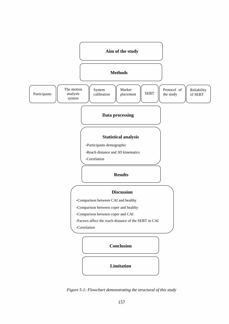
157

Figure ‎5-1: Flowchart demonstrating the structural of this study

Participants

Aim of the study

Methods

The motion

analysis

system

System

calibration

Data processing

Marker

placement

Statistical analysis

-Participants demographic

-Reach distance and 3D kinematics

-Correlation

-

SEBT

Results

Discussion

-Comparison between CAI and healthy

-Comparison between coper and healthy

-Comparison between coper and CAI

-Factors affect the reach distance of the SEBT in CAI

-Correlation

Conclusion

Protocol of

the study

Limitation

Reliability

of SEBT

158

5.3 Method

5.3.1 Participants

A total of 68 participants (33 male, 35 female) took part in the study. Participants

were classified into healthy, coper and CAI groups. The demographic data is presented in

Table 5.1. Participants were recruited from the University of Salford through advertisements

and flyers posted in the university. Before starting the test, all participants signed a written

consent form which was approved by the ethical committee of the University of Salford. The

inclusion and exclusion criteria were identical to those in chapter three. The study was

conducted in the gait laboratory at the University of Salford. Before the study, the researcher

prepared the laboratory by checking the connectivity of each camera, performing calibration

of the system, and preparing the markers for each participant.

Table ‎5.1: Demographic data of healthy, coper and CAI participants

Healthy

Mean ± SD

Coper

Mean ± SD

CAI

Mean ± SD

P-value,

effect size

Number of participants 28 18 22

Sex male/female 10/18 10/8 13/9

Years (y) 28.07 ± 6.32 28.53 ± 6.83 28.02 ± 7.71 0.95, 0.04

Weight (Kg) 68.46 ± 12.43 70.07 ± 15.41 69.73 ± 12.56 0.54, 0.14

Height (m) 1.68 ± 0.10 1.71 ± 0.09 1.69 ± 0.10 0.59, 0.10

BMI (kg/m²) 24.30 ± 3.19 24.00 ± 4.71 24.40 ± 3.64 0.85, 0.07

CAIT score 29.50 ± 0.70 27.53 ± 1.40a

13.62 ± 3.74a

<0.01, 3.04

Time since last injury

(months)

0.0 ± 0.0 18.12 ± 03.37 a,b

08.13 ± 2.83 a

<0.01, 3.21

Abbreviations: CAIT, Cumberland Ankle Instability Tool; BMI, Body Mass Index.

*Values are mean ± SD. a

Indicates statistical differences between CAI and coper, and between CAI and healthy

participants. b

Indicates statistical differences between coper and healthy.

5.3.2 The motion analysis system

Motion analysis includes particular techniques and procedures to systematically

analyse movement. Modern gait laboratories utilise motion analysis systems to describe

dynamic alteration in 3D coordinates of particular body landmarks from the images taken by

159

each camera. The 3D foot and ankle kinematic data (sample frequency 100 Hz) for this study

were recorded using twelve Qualisys infrared cameras (ProReflex, Qualisys Inc.,

Gothenburg, Sweden) that are permanently wall mounted to permit faster set up and

calibration. Four 400mm x 600mm force platforms (AMTI: Advanced Mechanical

Technology Incorporation, Watertown, USA, model BP4006001500) were embedded in the

middle of the gait laboratory to collect kinetic data at a frequency of 1000 Hz. In this study,

an in-ground force plate measured the kinetics of the ankle motions for‎ each‎ participant’s‎

foot.

The orientation of the force platforms and the positions of the motion capture cameras

are demonstrated in Figure 5.2. Qualisys proprietary software (Qualisys Track Manager

(QTM)) was utilised in order to connect the cameras. There are three steps in collecting the

kinematic data: calibration, data collection and 3D reconstruction of retroreflective markers.

Figure ‎5-2: Set up the gait laboratory with orientation of cameras and position of force platforms

5.3.3 System calibration

The aim of the calibration is to determine the accurate location of the markers in the

3D coordinate system utilising a direct-linear transformation (DLT) technique. The algorithm

for this technique builds a linear relationship between the 2D image and the real life 3D

coordinates of the markers (Grimshaw, Lees, Burden, & Fowler, 2006); each Qualisys

camera is synchronised and records a 2D (X and Y) image which is then rebuilt and presented

as a real life set of 3D (X, Y and Z) coordinates. It is important to ensure that the volume of

data is captured during calibration (Grimshaw et al., 2006). The location of the markers in 3D

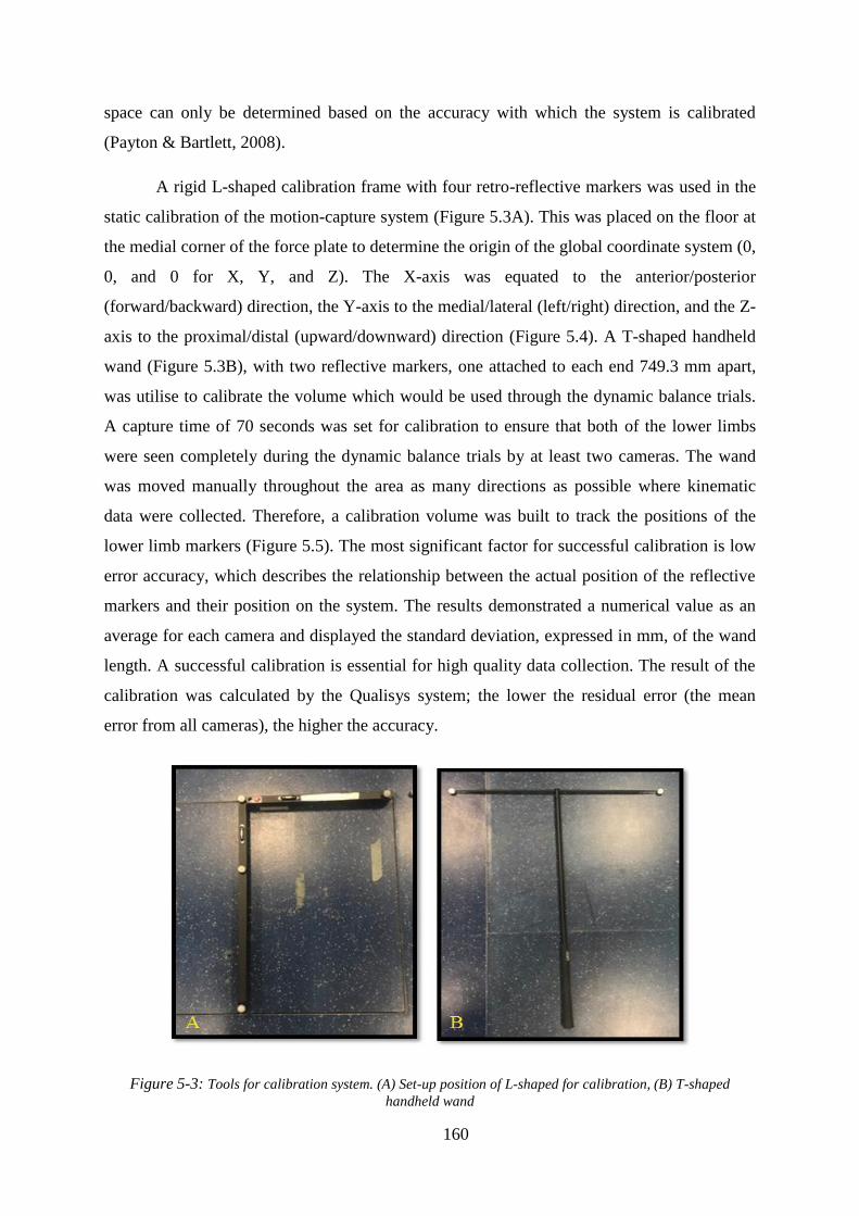
160

space can only be determined based on the accuracy with which the system is calibrated

(Payton & Bartlett, 2008).

A rigid L-shaped calibration frame with four retro-reflective markers was used in the

static calibration of the motion-capture system (Figure 5.3A). This was placed on the floor at

the medial corner of the force plate to determine the origin of the global coordinate system (0,

0, and 0 for X, Y, and Z). The X-axis was equated to the anterior/posterior

(forward/backward) direction, the Y-axis to the medial/lateral (left/right) direction, and the Z-

axis to the proximal/distal (upward/downward) direction (Figure 5.4). A T-shaped handheld

wand (Figure 5.3B), with two reflective markers, one attached to each end 749.3 mm apart,

was utilise to calibrate the volume which would be used through the dynamic balance trials.

A capture time of 70 seconds was set for calibration to ensure that both of the lower limbs

were seen completely during the dynamic balance trials by at least two cameras. The wand

was moved manually throughout the area as many directions as possible where kinematic

data were collected. Therefore, a calibration volume was built to track the positions of the

lower limb markers (Figure 5.5). The most significant factor for successful calibration is low

error accuracy, which describes the relationship between the actual position of the reflective

markers and their position on the system. The results demonstrated a numerical value as an

average for each camera and displayed the standard deviation, expressed in mm, of the wand

length. A successful calibration is essential for high quality data collection. The result of the

calibration was calculated by the Qualisys system; the lower the residual error (the mean

error from all cameras), the higher the accuracy.

Figure ‎5-3: Tools for calibration system. (A) Set-up position of L-shaped for calibration, (B) T-shaped

handheld wand

161

Figure ‎5-4: Illustration of the orientation of force platform

Figure ‎5-5: All the irregular cube- like shaped represent all spaces that has been calibrated

For a successful calibration, the manufacturer recommends that the value of the

residual error should be less than 1 mm (Grimshaw, 2006). The result of the average residuals

in this study was accepted as the values for all 12 cameras were < 0.8 mm, which mean the

locations of the markers in space were < 0.8 mm from their true positions.

To develop 3D coordinates, at least two cameras have to create a 2D coordinate set

for each marker. This procedure occurs for every time frame, following which the marker

trajectory is determined. These trajectories of the markers can therefore be applied for

kinematic analysis.

162

5.3.4 Marker placement

Lightweight spherical retro-reflective markers (14 mm and 9.5 mm in diameter)

(Figures 5.6A-B) were used to determine and track the anatomical segments. Karlsson and

Tranberg (1999) reported that the weight of the markers can create movement artefacts. Thus,

very lightweight markers were utilised in this study. A total of 30 anatomical markers were

used for each participant in order to determine anatomical reference frames of the shank, foot,

the centres of ankle and subtalar joint rotation. These markers were attached directly to the

skin by utilising hypoallergenic double-sided adhesive tape that was attached to a flat-based

marker. The ankle markers were attached to the medial and lateral malleolus; the foot

markers were placed on first, second and fifth metatarsal heads, and posterior heel, the cluster

(wand) markers were placed on calcaneal tubercle to tracked the calcaneus relative to the

shank which provide rearfoot eversion/inversion, while knee markers were placed on the

medial and lateral femoral condyle (Figure 5.8). Another four markers, known as cluster

markers, were attached to the four corners of the rigid polypropylene pads (Figure 5.7) that

were used for the shank segment. The shank segment was identified as a rigid structure

between the medial and lateral epicondyle of the knee joint proximally and the medial and

lateral malleolus of the ankle joint distally. The cluster pad was placed on the anterior lateral

of the shank and was fastened with an elastic strap to define the segment through the dynamic

balance movement. These clusters were used to decrease soft tissue artefacts through

movement (Cappozzo, Catani, Della Croce, & Leardini, 1995). Moreover, authors have

pointed out that the use of rigid clusters gives the optimal arrangement compared to

individual skin markers (Manal, McClay, Stanhope, Richard, and Galinat, 2000). Figure 5.8

illustrates the markers on a participant’s‎lower‎limb.

Figure ‎5-6: Types of markers. A: spherical retro-reflective marker, B: wand markers

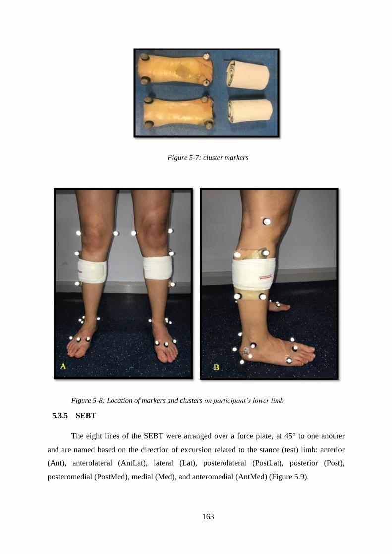
163

Figure ‎5-7: cluster markers

Figure ‎5-8: Location of markers and clusters on‎participant’s‎lower‎limb

5.3.5 SEBT

The eight lines of the SEBT were arranged over a force plate, at 45° to one another

and are named based on the direction of excursion related to the stance (test) limb: anterior

(Ant), anterolateral (AntLat), lateral (Lat), posterolateral (PostLat), posterior (Post),

posteromedial (PostMed), medial (Med), and anteromedial (AntMed) (Figure 5.9).

164

Figure ‎5-9: Eight directions of the SEBT. The directions are labelled based on the reach

direction in reference to the stance limb (Mahajan, 2017).

5.3.6 Protocol of the study

The study and the procedure for the test were explained to each participant clearly on

arrival, and the consent form was completed and signed. Once the participants completed the

ultrasound exam (described in detailed in chapter three), they had a rest for two-five minutes.

Then, the researcher began to place the retro-reflective markers on the lower limbs to start the

balance test.

The study began with the researcher asking the participants to complete a static trial

which include participants standing barefoot on the force plates. Each participant stood with

all of the markers attached to their lower limb, as described in the previous section (5.3.4), in

an upright position with their knee extended completely, their feet pointing forward towards

in anterior direction of the SEBT, and with both legs symmetrically positioned. The

participants were asked to remain in a static position for 20 seconds with their arms held

away from the markers to ensure that they did not cover them. This trial was conducted to

align the participant with the laboratory coordinate system and to record this as a reference

(zero degrees) position for further kinematic analysis (Fullam et al., 2014). The researcher

verified the placement of the markers and ensured that participants’‎movements‎were exactly

mimicked by the computer QTM software before starting the test.

Following the static trial, dynamic trials were measured during the SEBT. The

purpose of the SEBT is to reach with one limb as far as possible along each of the eight lines

165

designed by tape measures taped to the‎ laboratory‎ floor‎ (Figure‎ 5.10), whilst preserving

stability of the contralateral limb (Khuman et al., 2014). Both limbs were tested for the

comparison between injured and uninjured limb. The protocol for performing the SEBT was

taken from published practice (Doherty et al. 2015b; Gribble et al., 2012; Hoch et al., 2016;

Khuman et al., 2014). The instructions and the procedures for the SEBT were given verbally

to the participants by the researcher.

Figure ‎5-10: The eight directions of the SEBT with right limb stance

Participants started the test by placing the stance (test) limb on the middle of the

SEBT grid, while the untested limb was placed outside the force plate. They stood with their

hands on their hips for three seconds. They were then asked to reach as far as they could with

the non-weight bearing (untested) limb, making a light touch on the furthest point on the

measuring tape with the most distal part of the big toe, while maintaining appropriate control

of the standing limb. Participants leant backward during the performance this movement in

the AntLat and AntMed directions, and abducted the untested leg to the side of the body for

Lat reach distance (Lockie, Schultz, & Callaghan, 2016). For the PostLat and PostMed reach

distances, the participants leant forwards, adducting the leg to a position behind the body,

before extending the leg medially (Lockie et al., 2016). Examples of these excursions are

demonstrated in Figure 5.11.

166

Figure ‎5-11: Demonstration of SEBT directions with testing the left leg, (A)Anterolateral,

(B)Lateral, (C)Posterior, (D)Posteromedial, and (E)Anteromedial

Reach distance was measured by the researcher in centimetres using a one-meter

measuring tape extended from the middle of this grid in the relevant direction over the SEBT

(Appendix 17). Using the same technique, the researcher also took measurements for the

other seven directions. The participants were then asked to return the reaching limb to the

starting point and to stay still for three seconds. All trials were completed in sequential order

in either the counter clockwise (right limb) or clockwise (left limb) directions (Khuman et al.,

2014).

Following‎Pionnier’s‎(2016)‎techniques,‎the‎participants‎performed‎four practice trials

to decrease the learning effect and to become familiar with the SEBT grids, with a 30 second

167

break between each trial, then the average for the three trials in each direction were recorded

for analysis.

The motion of the foot and ankle structures in this study was quantified by applying a

technique known as Calibrated Anatomical System Technique (CAST) which was developed

by Cappozzo et al. (1995). The CAST was utilised to determine the six degrees of freedom

movement for each segment during the performance of dynamic tasks, involving three

rotations (sagittal, frontal and transverse) and three translations (anterior/posterior,

medial/lateral, and distraction/compression) (Cappozzo et al., 1995). This system develops an

anatomically related reference frame for the lower limb segments through the reflective

markers being placed on the external anatomical landmarks to give an external indication of

the orientations of the internal bones.

The trials had to be repeated in some cases of error. Errors involved: (1) a marker

falling off; (2) the stance leg losing normal contact or the heel lifting the force plate; (3) the

big toe not touching the tape or making a heavy or prolonged touch; (4) the hands changing

position or moving from the hips; (5) the participant losing balance or being unable to return

to the starting point in a controlled way (Doherty et al., 2015b).

As before any study, a reliability study was required to confirm that the researcher

could collect reliable data and to prove that the data could be repeated for the eight reach

distances of the SEBT. This will be discussed in the next section.

5.3.7 Reliability of the SEBT

Higher reliability of the SEBT has been previously reported on healthy recreational

athletes (Munro & Herrington, 2010). A reliability study of the SEBT was undertaken before

the main study conducted for both healthy and injured participants. This involved ten

participants who understood the aim and voluntarily consented to take part. The ten

participants (5 healthy, 5 injured), had a mean age of 27.20 ± 5.86 years, mean height of 1.67

± 0.11 m, mean weight of 68.17± 13.19 kg, and mean BMI of 24.33± 3.28 kg/m2. The

participants followed the protocol of the study [as described in the previous section (5.3.6)],

each performing the test twice, one week apart, with the same researcher in order to test the

intra-tester reliability.

The two-way mixed model with absolute agreement types of intraclass correlation

coefficient (ICC) and limits of agreement (LoA) were used to evaluate the reliability. The

data collected were analysed using SPSS. The descriptive characteristics of the measured

168

reach distances of the SEBT and their corresponding ICC and LoA values for healthy and

injured participants are listed in Tables 5.2-3. There was a good to excellent reliability for the

eight reach directions of the SEBT for the healthy participants, with ICC ranging from 0.87 to

0.99 and a limit of agreement between 2.20 and 14.5 % (Table 5.2). The reliability was also

excellent for the injured limb of injured participants, with ICC ranging from 0.91 to 0.99 and

limit of agreement from 3.68 to 14.6 % (Table 5.3).

The reliability of uninjured limbs for healthy and injured participants are presented in

Appendix 18. Examples of the Bland-Altman plot are demonstrated in Figures 5.12 and 5.13.

More plots for several directions for both healthy and injured participants are provided in

Appendix 19.

Table ‎5.2: Reliability and limit of agreement results for eight reach distances of injured limb in


Day 1

mean (SD)

Day 2

mean (SD)

ICC

(95% Confidence Interval)

95% LoA LoA

lower upper

Ant 86.78 (6.19) 86.05 (3.64) 0.92 (0.70-0.99) -5.43 7.07 14.50

AntLat 91.24 (2.06) 91.80 (1.30) 0.87 (0.62-0.95) -2.79 1.67 4.87

Lat 92.01 (3.47) 91.80 (3.56) 0.99 (0.91-0.99) -1.34 1.76 3.37

PostLat 97.02 (3.73) 96.40 (4.16) 0.93 (0.50-0.99) -3.46 4.70 8.44

Post 98.57 (3.89) 98.20 (3.42) 0.95 (0.60-0.99) -2.88 3.62 6.60

PostMed 91.26 (6.64) 90.85 (6.43) 0.99 (0.97-1.00) -0.59 1.41 2.20

Med 84.71 (2.22) 84.72 (2.57) 0.89 (0.30-0.98) -3.19 3.27 7.62

AntMed 85.92 (6.25) 84.20 (8.29) 0.95 (0.63-0.99) -4.24 7.68 14.00

Table ‎5.3: Reliability and limit of agreement results for eight reach distances of injured limb in

injured participants

DAY 1

mean (SD)

Day 2

mean (SD)

ICC

(95% Confidence

Interval)

95% LoA LoA

lower upper

Ant 74.58 (3.75) 74.38 (2.82) 0.97 (0.70-0.99) -2.29 2.69 6.68

AntLat 79.61 (4.55) 79.39 (5.12) 0.91 (0.60-0.99) -5.58 6.02 14.60

Lat 80.90 (5.62) 80.83 (6.26) 0.99 (0.94-0.99) -1.92 2.06 4.90

PostLat 81.64 (6.49) 81.60 (5.43) 0.98 (0.83-0.99) -3.29 3.37 8.16

169

Post 81.80 (6.85) 81.90 (6.43) 0.98 (0.91-0.99) -2.16 3.40 6.79

PostMed 82.45(5.18) 81.56 (5.21) 0.98 (0.71-0.99) -0.59 2.43 3.68

Med 69.08 (7.43) 68.39 (6.77) 0.98 (0.85-0.99) -3.30 4.68 11.61

AntMed 68.82 (4.79) 68.74 (5.29) 0.96 (0.68-0.99) -3.74 3.90 11.11

Figure ‎5-12: Bland and Altman plot for lateral direction of injured limb of healthy participant with

representation of limit of agreements

170

Figure ‎5-13: Bland and Altman plot for anterolateral direction of injured limb of injured participant

with representation of limit of agreements

5.4 Data processing

Because leg length is a significant factor in determining reach distance (Gribble &

Hertel, 2003),‎ each‎ reach‎ distance‎ was‎ normalised‎ to‎ the‎ participant’s‎ leg‎ length.‎

Normalisation of the reach distance was achieved by dividing the reach distance by limb

length and multiplying it by 100 (reach distance/limb length X 100 = % of limb length)

(Khuman et al., 2014). Therefore, the normalised value is expressed as a percentage of each

distance‎relative‎to‎the‎participant’s‎leg‎length‎(Pionnier et al., 2016); this percentage permits

a more precise comparison of the SEBT performance among participants (Gribble & Hertel,

2003).

The segments and planes were based on the recommendation of International Society

of Biomechanics. For the left and right foot (calcaneus, talus, cuboid, navicular, lateral,

medial, intermediate cuneiform, and metstarsal):

Of - The origin is located at the calcaneus landmark.

171

yf - The calcaneus and the first and fifth metatarsal heads define a plane that is quasi-

transverse. Orthogonal to this plane is quasi-sagittal plane which is defined by the calcaneus

landmark and the second metatarsal head. The intersection of these two planes is the y axis

and its positive direction is proximal.

zf – The axis lies in the quasi-transverse plane and its positive direction is from left to right.

xf - The axis is orthogonal to the yz plane with its positive direction is dorsal.

Cappozzo CAST model was also applied, which used clusters on the shank to track

movement. Then angles were calculated as flexion/ rotation – angle between shank and foot

at ankle axis in sagittal and transverse plane. The eversion/ inversion, were based on angle

between shank and calcaneus (calcaneus segments based on calcaneus markers/ foot position)

in the frontal plane.

The QTM software was used to label the 3D trajectory markers (Figures 5.14A-B).

The gaps in the data were completed to the maximum through applying a polynomial cubic

spline interpolation in QTM, which has the ability to refine the digitising errors of the markers

that could occur randomly during movement. The data were exported to C3D (Coordinate 3

dimensional) files in order to be imported into Visual 3D motion software (Version 6, C-

Motion, Inc., Rockville, MD) to calculate the ankle joint kinematic data. This software is

commonly used in studies calculating the kinematics of the lower extremity joints (Hsu et al.,

2014; Liu et al., 2012; Telfer, Abbott, Steultjens, & Woodburn, 2013;).

Bi-directional Butterworth low pass filters were applied with cut-off frequencies of 6 Hz

to smooth the kinematic data. This kind of filter permits low frequency data to pass but not high

frequency data, thus decreasing noise related to skin movement artefacts (Richards, 2008).

Foot and shank segment models (Figure 5.14C) were built to calculate the ankle joint

kinematic data. Kinematic data of the ankle (dorsi-plantar flexion, eversion-inversion,

internal-external rotation) were measured at the maximum reach distance in each direction of

the SEBT (Figure 5.15). The moment of maximum reach distance was defined as the

maximum difference between left and right foot segment centres. The averages for the three

trials for each kinematic variable were used for analysis. All of the data were exported as a text

file to Microsoft Excel to facilitate the analysis and presentation. For all kinematic variables,

positive values indicated dorsiflexion in the sagittal plane, inversion in the frontal plane, and

172

internal rotation in transverse plane. Negative values indicated plantar flexion in the sagittal

plane, eversion in the frontal plane, and external rotation in the transverse plane.

Figure ‎5-14: (A)QTM TM

static model and, (B) Labelling (C) Modelling

Figure ‎5-15: Image demonstrated the appearance of the posterior direction in visual 3D

5.5 Statistical analysis

A Shapiro-Wilk test was performed and demonstrated that the data was normally

distributed. This proves the appropriateness of parametric analysis. Several statistical

C

173

methods were used to answer the research questions and the analyses were conducting using

SPSS version 23 (SPSS Inc., USA), these methods are outlined below.

5.5.1 Participants demographic and questionnaires

The demographic variables (sex, age, weight, height, BMI, CAIT score) were

compared between healthy, coper and CAI participants using a one-way ANOVA. The

independent variable was group (healthy vs coper vs CAI). The significance level for the

analysis was set a priori at p< 0.05. If a significant difference was observed, the Bonferroni

post-hoc analysis was applied.

5.5.2 Reach distances and 3D kinematics

One-way ANOVA was applied for each reach direction of the SEBT to evaluate

whether there was a difference in reach distance and ankle motion between the groups

(healthy, coper, and CAI). If significant, a post-hoc (Bonferroni) pairwise comparison was

applied to determine the significant main pairwise effects. The independent variable was

group (healthy vs coper vs CAI), while the dependent variable consisted of the eight reach

distances and the ankle motions in the three planes. Moreover, paired t-tests were used to

compare left to right differences in each group. The significance level for the analysis was set

a‎ priori‎ at‎ p≤0.05.‎ Cohen’s‎ d effect sizes were calculated with d= 0.20 to 0.49 to be

considered a ‘small’ effect size, 0.50 to 0.79 representing a‎‘medium’ and‎˃‎0.80‎representing

a‎‘large’ effect size (McGough & Faraone, 2009).

5.5.3 Correlation between the thickness of lateral ligaments and anterolateral

direction of the SEBT

Pearson product-moment correlation coefficients were utilised to evaluate correlation

(r) and to characterise any relationship between changes in the thickness of ankle ligaments

(ATFL and CFL) in the three groups and the anterolateral direction of the SEBT for the three

groups. These relationships were described as weak (≤0.39), moderate (0.40–0.69) or strong

(≥0.70) (Lomax, 1998).

174

5.6 Results

5.6.1 Participants demographic and questionnaires

The demographic data for the three groups were homogenous at the baseline with p-

value >0.05, except for CAIT which showed significant differences between the groups with

p-value <0.01. Bonferroni post-hoc analysis demonstrated significant differences between the

healthy and CAI participants, between the healthy and coper participants, and between the

coper and CAI participants (p<0.01, p=0.02 and p<0.01 respectively).

5.6.2 SEBT reach distances

The within-group comparisons of injured and uninjured limbs of CAI participants

demonstrated significant differences in normalised reach distances in all eight directions of

the SEBT (p<0.05) except AntMed and Ant directions which demonstrated small to medium

effect size (Figure 5.16). There were no statistically significant differences in coper

participants between their injured and uninjured limbs in all eight directions with small effect

size in the Ant, AntLat and Lat directions of the SEBT (Figure 5.16). For healthy

participants, there were no statistically significant differences between both limbs. Therefore,

the side-matched ankle of healthy participants with injured ankle of coper and CAI was

selected for further analysis.

There were statistically significant differences in reach distances in all eight directions

between the three groups (p<0.05), with CAI participants achieving the shortest distances

(Figure 5.17). The Ant and AntLat reach distances were around 10% shorter in the CAI group

(74.2%, 77.9% respectively) compared to healthy participants (84.1%, 89.4% respectively)

(Figure 5.17).

There were also statistically significant differences in reach distances between healthy

and coper participants in the Ant, AntLat and Lat directions (Figure 5.17). Whilst there were

no significant differences in the PostLat, PostMed, Med and AntMed directions with only

small to moderate differences observed (Figure 5.17). However, the Post direction did not

show any significant differences between healthy and coper participants (Figure 5.17).

When comparing coper and CAI participants, there were statistically significant

differences in the AntLat, Post and Med reach distances (Figure 5.17). Whilst there were no

significant differences in the Ant, PostLat, PostMed and AntMed directions with small to

moderate differences observed (Figure 5.17). However, the Lat direction did not show any

significant difference between coper and CAI participants (Figure 5.17).

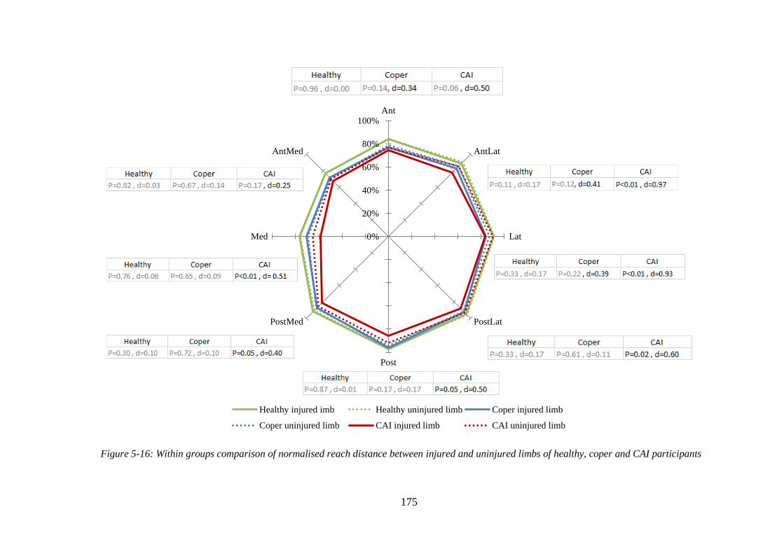
175

Figure ‎5-16: Within groups comparison of normalised reach distance between injured and uninjured limbs of healthy, coper and CAI participants

0%

20%

40%

60%

80%

100%Ant

AntLat

Lat

PostLat

Post

PostMed

Med

AntMed

Healthy injured imb Healthy uninjured limb Coper injured limb

Coper uninjured limb CAI injured limb CAI uninjured limb

176

Figure ‎5-17: Normalised reach distance of the SEBT of the injured limb of healthy, coper, and CAI participants

0.0%

20.0%

40.0%

60.0%

80.0%

100.0%Ant

AntLat

Lat

PostLat

Post

PostMed

Med

AntMed

Healthy Coper CAI

177

5.6.3 3D kinematics

The sagittal plane kinematics reflected a dorsiflexion movement in all eight directions

of the SEBT for all groups. In the frontal plane, there was eversion for all three groups in all

eight directions, except in the AntMed direction for healthy participants, for which there was

inversion. Regarding the transverse plane, there was internal rotation in all eight directions

for healthy participants. The coper and CAI participants also demonstrated internal rotation

for all eight directions, except in the AntMed direction, for which there was external rotation.

Figure 5.18 represents the differences in the kinematics of the ankle joint between the

three groups (healthy, coper and CAI) in each plane (sagittal, transverse and frontal). The

largest difference was seen in sagittal plane when compared to the frontal and transverse

planes. The differences in the sagittal plane were largest between healthy and CAI

participants with the AntLat direction being the most affected (p<0.01) (Figure 5.18). On the

other hand, the frontal plane was the smallest differences among the three planes (Figure

5.18). The descriptive values of the differences between the three groups in the three planes

are given in Appendices 20-22.

In the sagittal plane, CAI participants demonstrated a statistically significant decrease

in ankle dorsiflexion compared to healthy participants in all eight directions (p<0.05), except

in the Post and Med directions. Whilst, the effect size showed large effects for all directions

(Figure 5.18). Moreover, statistically significant decreases in ankle dorsiflexion were

demonstrated in the CAI participants compared to coper participants in the AntLat and

AntMed directions. Whilst, there was a moderate to large effect size in all eight directions

(Figure 5.18). Interestingly, there were no significant differences in ankle dorsiflexion

between healthy and coper participants in all directions; whilst, a small effect size was

demonstrated in the Ant, AntLat, Lat and PostMed (Figure 5.18). Figure 5.18 revealed that

the largest differences in ankle dorsiflexion were seen between healthy and CAI participants,

followed by coper and CAI participants, with no differences seen between healthy and coper

participants.

In the transverse plane, there was a statistically significant decrease in ankle internal

rotation between healthy and CAI participants in the Lat, Post and Med directions with a

moderate to large effect size was demonstrated in all eight directions (Figure 5.18). There

were no statistically significant differences in ankle internal rotation between coper and CAI

participants in all directions with a small to moderate effect in all directions, except in the

178

Ant and AntMed directions (Figure 5.18). There were no significant differences between

healthy and coper participants with only small to moderate differences observed in all eight

directions (Figure 5.18).

In the frontal plane, there were no statistically significant differences in ankle

eversion between healthy vs CAI, healthy vs coper, and coper vs CAI participants in all eight

directions (p>0.05) (Figure 5.18). Whilst, the effect size showed a small to moderate effect

between healthy and CAI participants in all directions except in the Ant and PostMed

directions (Figure 5.18). Furthermore, a small to moderate effect between coper and CAI

participants was found in all directions except the Ant, AntLat, and PostLat directions (Figure

5.18). There was also a small to moderate effect size between healthy and coper participants

in all directions, except the Med and AntMed directions (Figure 5.18).

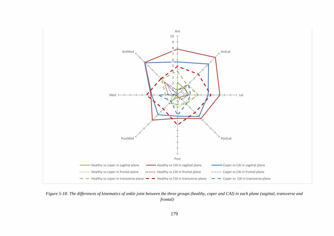
179

Figure ‎5-18: The differences of kinematics of ankle joint between the three groups (healthy, coper and CAI) in each plane (sagittal, transverse and

frontal)

0

1

2

3

4

5

6

7

8

9

10

Ant

AntLat

Lat

PostLat

Post

PostMed

Med

AntMed

Healthy vs coper in sagittal plane Healthy vs CAI in sagittal plane Coper vs CAI in sagittal plane

Healthy vs coper in frontal plane Healthy vs CAI in frontal plane Coper vs CAI in frontal plane

Healthy vs coper in transverse plane Healthy vs CAI in transverse plane Coper vs CAI in transverse plane

180

The within-group comparisons of injured and uninjured limbs for CAI participants

demonstrated a large significant difference in kinematics of the ankle joint in the sagittal

plane for all eight directions of the SEBT (p<0.01), except for the Med and AntMed

directions (p=0.06); whilst, the effect size showed a moderate effect in these directions

(Figure 5.19). Comparing the injured and uninjured limbs of coper participants showed no

statistically significant differences in the kinematics of the ankle joint in the sagittal plane

(p>0.05), except in the AntMed direction (p=0.04) (Figure 5.19); whilst, the effect size

showed a small effect in all directions except the PostLat, Post and Med. For healthy

participants, there were no statistically significant differences between injured and uninjured

limbs in all directions (p>0.05) (Figure 5.19).

Even though injured limb of CAI participants demonstrated a decrease eversion

compared to uninjured limb, it was only statistically significant different in the Lat and

PostLat directions of the SEBT, with large effect sizes (Figure 5.20). Whilst, the effect size

showed a small to moderate effect in all eight directions except, the AntMed direction. There

were no statistically significant differences between injured and uninjured limbs in coper and

healthy participants in the transverse plane (Figure 5.20). Whilst, a small effect size was

demonstrated in the Ant and Lat directions between injured and uninjured limbs among coper

participants (Figure 5.20).

Interestingly, there were no statistically significant differences in the kinematics of the

ankle joint between injured and uninjured limbs of the three groups in the frontal plane

(Figure 5.21). Whilst, there was a small effect size in the AntLat, Lat, Med and AntMed

directions for injured and injured limbs of coper and CAI participants (Figure 5.21).

Moreover, a small effect size was demonstrated in the PostLat and Post directions between

injured and injured limbs of healthy participants (Figure 5.21).

181

Figure ‎5-19: Kinematics of ankle joint for injured and uninjured limbs in healthy, coper, and CAI participants in sagittal plane

0

5

10

15

20

25

30

35

Ant

AntLat

Lat

PostLat

Post

PostMed

Med

AntMed

Healthy injured limb in sagittal plane Healthy uninjured limb in sagittal plane Coper injured limb in sagittal plane

Coper uninjured limb in sagittal plane CAI injured limb in sagittal plane CAI uninjured limb in sagittal plane

182

Figure ‎5-20: Kinematics of ankle joint for injured and uninjured limbs in healthy, coper, and CAI participants in transverse plane

-2

0

2

4

6

8

10

12

14

16Ant

AntLat

Lat

PostLat

Post

PostMed

Med

AntMed

Healthy uninjured limb in transverse plane Healthy injured limb in transverse plane Coper injured limb in transverse plane

Coper uninjured limb in transverse plane CAI injured limb in transverse plane CAI uninjured limb in transverse plane

183

Figure ‎5-21: Kinematics of ankle joint for injured and uninjured limbs in healthy, coper, and CAI participants in frontal plane

-10

-8

-6

-4

-2

0

2Ant

AntLat

Lat

PostLat

Post

PostMed

Med

AntMed

Healthy uninjured limb in frontal plane Healthy injured limb in frontal plane Coper injured limb in frontal plane

Coper uninjured limb in frontal plane CAI injured limb in frontal plane CAI uninjured limb in frontal plane

184



Since the previous results have demonstrated that reach distance in the AntLat

direction of the SEBT is the most affected, a correlation was calculated for this direction.

Figures 5.22 and 5.23 showed that the thickness of the ATFL and CFL had a significant

moderate correlation with the AntLat direction of the SEBT (r = -0.53, p<0.001and r = -0.40,

p<0.001 respectively).

Figure ‎5-22: Pearson correlation between anterolateral reach distance on the SEBT and thickness of

ATFL of the involved limb for healthy, coper, and CAI groups. The trend line symbolises the overall

correlation for the three groups

Figure ‎5-23: Pearson correlation between anterolateral reach distance on the SEBT and thickness of

CFL of the involved limb for healthy, coper, and CAI groups. The trend line symbolises the overall

correlation for the three groups

500

600

700

800

900

1000

1.6 2.1 2.6 3.1An

teri

ola

tera

l r

each

dis

tan

ce

(mm

)

ATFL Thickness (mm)

R2 = 0.28

500550600650700750800850900950

1000

1.4 1.6 1.8 2 2.2An

teri

ola

tera

l r

each

dis

tan

ce

(mm

)

CFL Thickness (mm)

R2 = 0.16

185

5.7 Discussion

5.7.1 Comparison of the reach distance of the SEBT between CAI compared to


Capturing the deficits that participants report related with CAI in measurable

laboratory test is important for the development of objective outcomes for diagnosis,

prognosis, and rehabilitation. The most significant finding was that participants with chronic

ankle instability demonstrated poorer dynamic balance than healthy participants in all eight

directions of the SEBT. As a result from the ultrasound study (chapter three), the length,

thickness of ATFL and the thickness of CFL were greater in CAI participants compared to

healthy participants. This demonstrated both mechanical instability and structural adaptations

occur in participants with CAI who exhibited in shorter reach distances.

The anterior directions of the SEBT (anterior, anterolateral, and anteromedial)

demonstrated great differences than the posterior directions (posterior, posterolateral, and

posteromedial) in CAI compared to healthy participants with the anterolateral direction was

the most significantly difference, followed by the anterior direction. This result agrees with

those seen by Ahn, Kim, and Kim (2011) and Doherty et al. (2016) who found the anterior

directions were shorter than posterior directions in CAI participants compared to healthy

participants. Olmsted et al. (2002) and Pionnier et al. (2016) also found that CAI participants

had significantly shorter reach distances than healthy participants when standing on the

injured limb. However, both studies averaged the scores for all eight reach distances; their

analyses did not treat each direction independently. It could be that they averaged the scores

for all eight directions as they aimed to test the efficiency of the SEBT in detecting dynamic

balance deficits in participants with CAI. Several studies used three directions (YBT) instead

of the eight directions of the SEBT (Doherty et al., 2016; Plante & Wilkstrom, 2013). Payne

et al. (2016) compared distances during the YBT (anterior, posteromedial, and posterolateral)

among soccer players with and without CAI. The result demonstrated that the anterior

direction was the only difference between these groups.

In ankle joint motion, dorsal flexion and plantar flexion were defined as rotation

around the medial-lateral axis, inversion and eversion were defined as around a rotation

around the anterior-posterior axis, and external and internal rotation were defined as rotation

around the proximal-distal axis (Fong, Chung, Chan & Chan, 2012).

186

Gabriner and colleagues (2015) studied the contributions of the ankle dorsiflexion

range of motion, strength, static postural control and plantar cutaneous sensation to the

performance of the YBT in chronically unstable ankles. They found that ankle dorsiflexion

range of motion and plantar cutaneous sensation contribute to 16% of the difference related to

anterior direction, and eversion strength and time-to-boundary mean minima (TTBMM) in

the medial-lateral direction contribute to 28% of the difference related to posteromedial.

Their results suggested different physical demands required to perform the anterior and

posterior directions of the SEBT which could explained the differences found in the present

study. The anterior direction might be more affected by sensory deficits and mechanical

restrictions at the ankle complex, while the posterior directions depend more on the postural

control and strength (Gabriner et al., 2015). This result emphasised Terada‎ et‎ al.’s (2014)

finding that mechanical restriction (smaller dorsiflexion ROM) at the ankle affect only the

anterior direction of the YBT in participants with CAI.

Another possible explanation of the anterior directions being most affected than

posterior directions could be due to different of muscle activity in each direction. Feger and

colleagues (2014) studied the activation of the lower limb muscles during YBT for

participants with and without CAI. They found that CAI participants showed less activity of

the ankle, knee and hip musculature during YBT compared to healthy participants which

decrease the angles of hip and knee flexion. Thus, the ankle joint instability is influenced by

the impairment of neuromuscular adaptation of the knee joint caused by decrease the torque

of the ankle plantar flexor and knee flexor and extensors (Gribble & Robinson, 2009).

Most of the ankle sprains create injury to the lateral ligaments (also reported in our

ultrasound study). Ahn et al. (2011) found that functionally unstable ankles had weaker

plantar flexors compared to healthy group. The electromyography (EMG) activities of

peroneal longus, tibialis anterior, and biceps femoris were also significantly lower compared

to healthy participants in the anterior, anterolateral, and anteromedial directions of the eight

directions of the SEBT. Although, peroneus longus muscles, play a significant role in

controlling ankle inversion, there were no significant differences in the thickness and the

CSA in CAI participants compared to healthy and copers (as demonstrated previously in

chapter 3), suggesting that the peroneals may have similar structure, yet, functionally act

differently when controlling movement. Ahn et al. (2011) reported tibialis posterior and

soleus activation was lower in the posterior, posteromedial and posterolateral while vastus

lateralis activation was lower in the lateral direction. The EMG differences between different

187

reach distances could assist clinicians to decide which reach directions to apply as outcome

measures in patients with particular deficiency in the muscle strength. The tibialis posterior

must be strengthened rather than strengthened peroneus longus. Thus, strengthened invertor

as well as evertor must be desired for preventing the ankle instability. The results suggest that

preventing the reoccurrence of ankle sprain can be occur by strengthened muscles

contributing to the ankle stabilisation specially in the anterior directions and activation feed-

forward motor control by the analysis of muscle activities involved based on the SEBT in

CAI.

In contrast to the current and previous research, De La Motte et al. (2015) studied the

medial reach distances (anteromedial, medial, and posteromedial) between healthy and CAI

participants and found no statistically significant differences in these three directions (p=0.66,

p=0.35 and p=0.45 respectively). These results are similar to those reported by Sefton et al.

(2009), who also found no differences in these three reach distances in CAI participants

compared to healthy participants. Furthermore, Razeghi et al. (2016) studied the ability of the

YBT (anterior, posteromedial and posterolateral) to differentiate between women with and

without CAI. They found no statistically significant differences in the three directions

(p>0.05) between the two groups. These studies emphasised the need to perform eight

directions of the SEBT instead of only three directions when testing participants with

previous history of ankle sprain. Since some of the SEBT directions could not be sensitive

enough to detect the deficiency and based on our result AntLat direction was the most

significant different between the three groups and it was not test in these previous studies.

Stiffness of the lateral ligaments and weakness of the muscles that are in charge for

eversion and pronation of the ankle complex contributes to functional instability in the lateral

ankle sprain. Changes in the structures can possibly reduce the ankle dorsiflexion which

restrict the movement of the ankle joint and decrease the reach distance in participants with

CAI. The movement of the ankle joints during the SEBT was measured by using the motion

analysis system. Biggest differences between the groups were seen in the sagittal plane, with

the differences between CAI and healthy participants being the most affected, particularly in

the anterior directions (anterior, anterolateral and anteromedial). In other words, ankle

dorsiflexion was most significantly decreased in CAI participants, this outcome supports the

evidence that limitation in ROM is contributing factor in individuals with CAI (Collins, Teys,

& Vicenzino, 2004; Morrison & Kaminski, 2007). Moreover, the smallest difference in the

sagittal plane (dorsiflexion) occurred in the posterior direction, which could also reflect the

188

fact that the CAI participants was able to achieve longer reach in the posterior direction of the

SEBT than in the anterior direction, as discussed previously. Using the kinematic in this

study helps to explain the shorter reach distance demonstrated in CAI.

Many studies support the findings of this study and have observed a restriction in

ROM after an ankle sprain and commonly in dorsiflexion (Collins et al., 2004; Hubbard &

Hertel, 2006). It has been reported that stiffness of the gastrocnemius and soleus muscles can

create restrictions in dorsiflexion (Denegar & Miller, 2002). This plays a role in abnormal

movement during physical activity, which could affect the tissue around the ankle in

generating a compensatory movement in order to maintain function (Almansour, 2015).

Therefore, this will predispose the individual to a high risk of sustaining another sprain

(Hubbard & Hertel, 2006).

Doherty et al. (2015b) evaluated the 3D kinematics of the joints of the lower

extremity during the performance of the YBT in participants within two weeks of having a

first time lateral ankle sprain and in a control group. Sagittal plane kinematic profiles

demonstrated decreased flexion displacements at the hip, knee and ankle during reach

performance. In addition, the frontal plane of the ankle joint showed a decreased eversion

displacement in the posteromedial direction only which contradict our findings in which there

was no difference in the frontal plane between the groups.

In a follow-up study, Doherty et al. (2015a) conducted a study on participants within

six months after their initial acute sprain to measure the sagittal plane kinematics of the lower

limb at the point of maximum reach distance in the YBT by using 2D video analysis. The

injured limb of the lateral ankle sprain participants presented with decreased hip and knee

flexion, and ankle dorsiflexion in all three directions compared to healthy participants.

Doherty et al. (2016) repeated the study in CAI and coper participants within one year after a

first time lateral ankle sprain. They found that CAI participants showed decreased hip and

knee flexion in posteromedial direction compared to coper and healthy participants. While

CAI participants demonstrated decreased knee flexion and ankle dorsiflexion displacement

only in the posterolateral direction compared to coper and healthy participants.

In recent research, Pionnier et al. (2016) found that, in addition to decreased medial

rotation of the hip and knee, ankle pronation/supination and abduction/adduction ROM were

reduced in CAI participants compared to healthy participants (p<0.01 and p=0.04

respectively). However, there was no statistically significant difference in ankle

189

flexion/extension between CAI and healthy participants (p=0.45). The results from Pionnier

et al.’s (2016) study revealed that the ROM in CAI participants decreased, especially in the

transverse and frontal planes, reducing medio-lateral restraints at the ankle joint, and

therefore limiting stresses on the lateral ligaments (Pionnier et al., 2016). A possible

explanation for the differences in ankle dorsiflexion ROM in the reach directions between the

present study and the previous studies could be the differences in inclusion criteria used for

CAI participants. For example, in Pionnier et al.’s (2016) study, CAI participants should have

had at least one sprain and at least three episodes‎ of‎ “giving-way”.‎ In‎ addition,‎ different‎

directions of the SEBT used in different studies.

The present study also demonstrated significant differences in transverse plane

between CAI and healthy participants. In addition, it seems that CAI and coper participants

adopt different strategies to healthy participants in the AntMed direction. Their ankles

demonstrated an external rotation, while healthy participants performed an internal rotation

motion. Interestingly, it seems that all three groups (healthy, coper and CAI) rely least on the

frontal plane during the performance of the test. This finding reflected De la Motte et al.’s

(2015) previous finding that CAI participants may use various movement strategies that could

be reliant more on motion in the transverse or frontal planes to achieve the movement goal. A

possible explanation for those with CAI adopting transverse strategies is the limitation in

ankle dorsiflexion range of motion which is frequently recognised in these people (Hoch et

al., 2012).

Cumulatively, the alteration and deficits in proximal muscles and controlling of the

joint as well as stereotypical movement patterns demonstrate global deficits in sensorimotor

function. This study demonstrate the need of better and longer protective of ankle joint

following an acute sprain to assist restore mechanical stability. Increased the laxity of the

ligament can produce further mechanical adaptation, impairment in controlling the

sensorimotor, ankle sprain reoccurrence, and reduction in global function as maladaptive

compensation of the change in joint laxity and/or sensorimotor control.

5.7.2 Comparison of the reach distance of the SEBT between coper and healthy

participants

Few researchers have conducted studies that include copers in addition to CAI and

healthy participants (Doherty et al., 2016; Plante & Wilkstrom, 2013). Even though coper

participants did not develop CAI, the present study showed that they are quit differ from

190

healthy participants. They reported a decrease normalised reach distance in the anterior,

anterolateral, and lateral directions of the SEBT compared to healthy participants (p<0.05).

Whilst, there was a small to moderate (d=0.36 – 0.62) difference in the remaining directions

except the posterior direction. This difference between coper and healthy participants is

consist with structural change in the thickness of ATFL that found in the ultrasound study.

These results shad the light that copers could go to the same way as CAI, however, it is not

sever enough to develop CAI. In contrast to the present study, Plante and Wilkstrom (2013)

and Doherty et al. (2016) did not find differences in the YBT between coper and control

participants. However, they only tested three directions which may not be sensitive enough to

detect the deficiency.

Even though there was no statistically significant difference in the kinematics data

between the coper and healthy participants, lateral ligament structure and reaching distance of

the coper demonstrated significant different. It seems that copers are a high risk to develop

CAI as their structural and functional of the ankle joint are not perfectly well as healthy

participants. Therefore, it is suggested that a rehabilitation plan can be drawn which include

selective muscle strengthening for coper participants to avoid further disability and develop

CAI.

5.7.3 Comparison of the reach distance of the SEBT between coper and CAI

participants

When comparing coper and CAI participants, normalised reach distances were

significantly decreased in the anterolateral, posterior and medial directions with a small to

moderate (d=0.39 – 0.53) effect size in the remaining directions except the lateral direction.

The differences in balance between coper and CAI participants in the present study are

consistent with previous studies (Wikstrom, Fournier, & McKeon, 2010a; Wikstrom et al.,

2010b) in which deficits in static and dynamic balance were found. Therefore, it seems that

impaired balance is a significant consequence of CAI that most probably has significant

negative consequences for functional performance (Plante & Wikstrom, 2013) as

demonstrated by the fact that balance deficit is related to increase the risk of ankle injury

(Wang et al., 2006). Furthermore, differences between coper and CAI participants in some

directions suggest that this result could represent a side of the coping mechanism that is

absent in CAI participants.

191

Changing kinematic patterns have been reported previously in people with ankle

instability during the performance of more dynamic jumping and landing tasks (Brown,

Padua, Marshall, & Guskiewicz, 2011; Caulfield & Garrett, 2002). Caulfield and Garrett

(2002) proposed that these changes may point to a learned adoptive strategy as a consequence

of previous injury and could be reflected in other tests in which CAI dysfunction is presented.

These learned strategies may assist in elucidating the finding of this present study in each of

the eight directions between the groups. SEBT is a close chain exercise which permits

participants to achieve the reach distances in a self-selected manner at a self-selected pace

(De La Motte et al., 2015). Therefore, it could be that the coper and CAI participants in the

current study have utilised a learned adaptive compensatory motor-control strategy,

representing a change in the sagittal plane kinematics of the ankle during the performance of

the SEBT test.

Even though the present study showed a significant difference of ankle dorsiflexion at the

anterior directions only, Plante and Wilkstrom (2013) and Doherty et al. (2016) found a

difference in posterolateral reach distances between coper and CAI participants. However,

coper participants in Doherty et al.’s‎(2016) study had their sprain for exactly one year and

achieved better reach distances than those in the previous studies already mentioned. For

instance, the mean reach distance for coper participants in the PostLat direction was (99.80 ±

8.70 %) which is significantly higher than the finding in the present study and in Plante and

Wilkstrom’s‎ (2013) study (92.6 ± 8.40 %, 83.0 ± 8.0 % respectively). It could be that the

participants in Doherty et‎al.’s‎(2016) study represent a population who are at an early stage

of the disease process; it is possible that the pattern of ankle instability becomes worse with

time (Doherty et al., 2016). Meanwhile, participants with years of ankle instability are

specifically prone to time-dependent deteriorations in functional capability, as might have

been the situation in the present and previous studies (Hertel et al., 2006; Hoch et al., 2012;

Plante & Wikstrom, 2013); it is improbable that a precise one-year cut-off occurs whereby

the degenerative ankle instability process reach relative stasis (Doherty et al., 2016).

Moreover, Jaber et al. (2018) found a higher activation of the anterior tibialis and

gluteus maximus in coper and healthy participants might be explained as a strategy utilised

by these groups to maintain the stability in case of more challenge task such as anterior and

posterolateral direction. Therefore, the poorer achievement demonstrated in CAI participants

during these directions may be attributed to the lack of such strategy. Moreover, coper and

healthy participants utilised both ankle and hip muscles during the posterolateral direction

192

while CAI participants depends more on the ankle muscles to complete the task. Furthermore,

Jaber et al. (2018) found that CAI participants demonstrated a significantly delayed in only

gluteal muscles activation onset time but not in the ankle muscles. This dependence on ankle

strategy to maintain stability could be considered a suboptimal muscle recruitment pattern

and it might clarify the higher injury risk in people with CAI.

Even though the YBT has commonly been used in studies, Coughlan and colleagues

(2012) argued that various strategies for postural control could be utilised to perform this test.

Therefore, it is difficult to directly compare the current finding with previous findings from

using the YBT or from using only the medial directions of the SEBT. This is because it is

also demonstrated in this study that each direction could represent a different movement

strategy for each group. For instance, during reach movement in the anterior direction in the

transverse plane, the greatest difference was between healthy and coper participants while the

smallest difference was between coper and CAI participants. However, in the posterior

direction, the opposite occurred, with the biggest difference being between the coper and CAI

participants and the smallest between coper and healthy participants. This means that coper

participants were able to adapt a strategy similar to healthy participants in the posterior

direction but not in the anterior direction, which is similar to CAI. This finding could also

explain why the coper participants were able to achieve better reach distances in the posterior

than the anterior direction. Coper participants in this study demonstrated no significant

differences at the ankle joint compared to healthy and CAI participants in transverse and

frontal planes, this explained that coper participants could rely more on proximal joints and

muscles which need a further investigation.

Therefore, it seems important to investigate the three kinematic planes along with the

eight directions of the SEBT in order to complete understanding functional consequences of

lateral ankle sprain. All of these findings can point to an adaptation in the central nervous

system, which sets up a protective motor command relying on previous experiences of lateral

ankle sprain or ‘‘giving-way’’‎of‎the‎ankle. This motor adaptation could decrease the risk of

ankle instability which can be induced by whole body-wide movements or accelerations

(Pionnier et al., 2016).

5.7.4 Other factor could affect the reach distance of the SEBT in CAI participants

Interestingly, it has been reported that participant apprehensiveness could be the most

crucial factor in inhibiting performance (Olmsted et al., 2002). It could be that after

193

sustaining their injury, many participants are hesitant in attempting to accomplish the SEBT

which asks them to challenge their limits of stability. Olmsted et al. (2002) reported that

many participants with CAI in their study experienced a feeling of apprehension while

reaching in a specific direction of the SEBT and trying to keep their injured limb stable.

However, in a quiet standing balance test apprehension does not play a significant role,

because participants are rarely required to challenge their limits of stability (Olmsted et al.,

2002).

5.7.5 Differences of reach distance of the SEBT between anterior and posterior

directions in healthy participants

The posterolateral and posteromedial directions were significantly longer than the

anteromedial and anterolateral directions. A possible explanation for this could be that

muscle activation differs in each direction. Earl and Hertel (2001) demonstrated that muscle

activation (measured using EMG), was significantly different during movement in the eight

different reach directions of the SEBT for healthy participants. Reach distance is therefore

sensitive to direction. They reported that during the performance of the three anterior reaches

of the SEBT, the quadriceps were the most active muscles in the lower limbs, with the vastus

medialis being the most active in the anterior reach direction compared to all other directions.

In addition, the medial hamstring showed greater activity in the anterolateral direction than in

the other anterior directions (Earl & Hertel, 2001). During the performance of posterior reach

distance, the anterior tibialis was the most active muscle. The activity of the biceps femoris

was greater in the posterior, posterolateral and lateral directions compared to the anterior and

anteromedial directions (Earl & Hertel, 2001). Based on these findings, it seems that the

activity of the lower extremity muscles is reach dependent.

5.7.6 The inconsistency of the results between this study and previous studies

This inconsistency in the results for reach distances and kinematic data in the SEBT

between CAI and healthy participants, coper and healthy participants, and coper and CAI

participants between the previous studies may be due to numerous differences in inclusion

criteria, statistics and methodology, such as variations in the number of practice trials. Some

studies asked the participants to perform six practice trials (De La Motte et al., 2015) while

other required three or four trials. Moreover, hand placement was not consistent among the

previous studies. In the present study, along with several previous studies, (De La Motte et

al., 2015; Doherty et al., 2016) the participants positioned their arms on the iliac crest of the

194

waist during each trial to avoid supporting their balance with their hands. On the other hand,

in Earl and Hertel’s (2001) study, the participants were allowed to move their arms freely.

This free arm movement made the task of maintaining balance less challenging by increasing

the counterweight moment while performing the reach distance and therefore changing the

function of the muscles (Anderson, 2016). In addition, the inclusion criteria could also

explain the differences in findings. As it generate heterogeneous sample of participants which

limits our ability to compare the results across different studies. Even though all studies need

an ankle sprain for inclusion, the severity, the number of the sprain, and the time since last

injury could be different. It is assumed that participants with many sprains or regular episodes

of ankle giving way had increased ankle disability and decrease function compared to

participants with only a feeling of giving away. In addition, it is important to recognise the

time since last injury because an early stage after most recent ankle sprain could affect the

results of the study as full recovery may have not taken place and the deficits occur could be

due to the consequences of acute phase (Delahunt et al., 2010).



In addition to any changes in the associated muscles and tendons of the ankle joint,

which may simply reduce active ROM, potentially due to disuse post injury, the findings

indicate that participants with thicker ligaments achieved shorter distances in the SEBT. One

possible explanation for this is that thicker ligaments are stiffer and restrain joint motion,

therefore prevent longer reach distances as kinematic data demonstrated decrease in the

dorsiflexion ROM of coper and CAI participants compared to healthy participants.

It is assumed that changing morphology of the ligament influences the stability of the

ankle and thereafter the ability to control balance during reaching movements that involve

joint motion placing the thicker ligaments under strain. In addition, the skeletal muscle and

tendons will also play a role during the dynamic tasks. If however thicker ligament infers

more compliant structure, perhaps due to greater water content, or disorganised collagen

fibres post healing, then deficiency in maintaining balance occur and participants with injured

ankles are not able to achieve long reach distance as healthy ankles.

195

5.8 Limitation

Even though the study evaluates the three planes of movement for the eight directions

of the SEBT, it has only evaluated the ankle joint. It should be acknowledged that the hip and

knee joints are involved in the performance of the SEBT. As such, future study should

evaluate the kinematics of the whole lower extremity of healthy, coper and CAI participants

and to include coordination training for the whole lower limb into rehabilitation following

lateral ankle sprain. Moreover, the researcher did not measure the EMG of the lower

extremity muscles which related to the performance of SEBT and could provide additional

insight to reach distance behaviour during the SEBT. Even though the demographic data

(age, height, weight, and BMI) was matched between the groups, the number of male and

female participants in each group was differ and future researches should assess a single

gender to reduce the possibility of the effect of gender in the test performance.

5.9 Conclusion

Differences in dynamic balance exist between CAI and healthy participants in all

eight directions of the SEBT, coper and healthy participants in the anterior, anterolateral, and

lateral directions, and CAI and coper participants in the anterolateral, medial, and posterior

directions.

The differences in reach strategies were mainly in the sagittal plane which greater

decrease dorsiflexion motion/angle in the CAI participants compared to coper and healthy

participants, and during all directions except medial and anteromedial directions of SEBT.

This study also provides an insight into the negative relationship between the thickness of

ankle ligaments (ATFL and CFL) and the anterolateral reach distance in the SEBT.

196

6 Chapter six: Overall summary, conclusion, limitation and

recommendations for future work


This final chapter starts with an overall summary of the thesis. A brief discussion of

the lack of detailed sonographic studies and quantitative analysis of the echogenicity and

literature on ankle sprain are included as a reminder of the rationale for the thesis. The

novelty of this work is also highlighted, limitations, clinical relevance and recommendations

for future work presented.

6.2 Overall summary of the thesis

The ankle is considered one of the most traumatised body sites and accounts for 3-5%

of all admissions to hospital emergency rooms in the UK. Sprains account for approximately

85% of all ankle injuries with the lateral ankle ligaments the most frequently injured site.

Physical examination of the anterior drawer and talar tilt tests assist in defining the extent of

injury, especially in most severe injuries. However, these tests are subjective and appear to be

unreliable. Imaging of the foot and ankle area help in diagnosis, therapeutic decision-making,

and evaluation of functional results. Foot and ankle structures have been scanned using plain

radiographs but these are not helpful in ligamentous sprains and poor utility of x-rays led to

the‎development‎of‎the‎“Ottawa Ankle Rules”, as a means to help management of acute ankle

injuries. On the other hand, MRI is considered to be the gold standard for diagnosing the

ankle ligaments after ankle sprain, but access can be limited. Using musculoskeletal

ultrasound to detect ankle abnormalities has revealed positive findings in relation to make

sprains and more screening of the precise soft tissue injury may help inform the design of

individual intervention programmes.

The review of the literature (chapter two) identified a knowledge gap regarding our

understanding of ankle structures in people with previous ankle sprain, specifically between

those who develop further ankle sprains after the first, and individuals who do not report any

complications after the first sprain. This is important because it may improve our

understanding of whether structural features of the injury explain why some individuals

experience ongoing ankle instability while others do not. However, it is also important to ask

how changes in any structural features may affect the functional performance of the ankle.

197

The first aim of this PhD thesis was to characterise and compare selected ankle

structures in people with and without a history of ankle sprain. The second study was aimed

to provide a quantitative analysis of echogenicity of the anterior talofibular ligament in

healthy, coper and CAI participants using computer-aided greyscale analysis software. The

last study was aimed to investigate the dynamic balance in people with and without a history

of ankle sprain. To achieve these aims, the thesis was conducted in three studies.

The study presented in chapter three was designed to investigate structural changes in

selected ankle structures in people with and without previous ankle sprain. An ultrasound

protocol was developed to assess the length, thickness and cross sectional area of ATFL,

CFL, peroneal tendons and muscles, TPT and AT. ATFL was found to be longer and thicker

in both coper and CAI participants compared to healthy and thicker but not longer in CAI

compared to copers. An interesting finding among healthy participants was that overweight

participants demonstrated thicker and larger CSA of most of the selected ankle tendon and

muscles compared to normal weight participants that is likely due to the additional strain

placed on these structures.

In addition to the thickness and the length of the ATFL, it was important to

characterise the ligaments in term of echogenicity to have a great understanding of the

structural changes. Injured ligaments were defined‎in‎the‎literature‎as‎“hypoechoic”‎which‎is

considered to be a qualitative definition, and it does not give any absolute quantitative

information related to the degree of echogenicity. Therefore, there was a need to quantify the

echo intensity in order to objectively characterise and compare the ATFL in healthy, coper

and CAI participants. Since ultrasound image included different value of echo intensity,

computer-aided greyscale analysis software was used in chapter four in order to provide

numerical data of the ATFL intensity which overcome the limitations of qualitative and

subjective definitions of the echogenicity. The intensity of the ATFL was lowest in CAI

following by coper then healthy participants. Ultrasound evaluation of selected ankle

structures could improve the ability of the clinician to determine the current situation of the

ligaments injury and produce more knowledgeable treatments and rehabilitation decisions

regarding each individual.

While the previous studies (chapter three and four) characterise structural changes,

they do not provide any insight into the functional consequences of any changes. Functional

deficits were investigated using the SEBT whilst limb kinematic and kinetics were

198

monitored, and compared between healthy and injured ankles. Results demonstrated poorer

performance of the balance test, in all eight directions, in CAI participants compared to coper

and healthy participants, poorer performance of the balance test in anterior, anterolateral and

lateral directions in copers compared to healthy participants. In addition, significant

differences were found in ankle kinematics between the three groups. The findings

demonstrate decreased ROM mainly in the sagittal plane in CAI participants compared to

coper and healthy participants.

Since the thickness of ATFL and CFL were the most structurally significant different

among the three groups and the anterolateral reach distance of the SEBT was the most

functionally significantly different, a correlational analysis was conducted to evaluate the

association between the thickness of the ligaments (ATFL and CFL) and the anterolateral

reach distance of SEBT. The study showed that the thickness of ATFL and CFL had a

significant negative moderate correlation with anterolateral direction of SEBT (r = -0.53,

p<0.001 and r = -0.40, p<0.001 respectively), as the thickness increased, the reach distance

decreased.

6.3 Thesis novelty

This thesis has added to the literature on ankle sprain, highlighting the importance of

accounting for the differences in length and thickness of lateral ankle ligaments post injury.

Characterise selected ankle structures in people with and without a history of ankle sprain has

been quantified for the first time. Throughout this work differences between healthy, coper

and CAI participants have been identified. CAI participants demonstrated longer and thicker

ATFL and thicker CFL compared to coper and healthy participants. The thickness of ATFL

was also thicker in coper compared to healthy participants. CAI participants had the lowest

ATFL echogenicity and coper participants had lower than healthy. Regarding functional

consequences of ankle sprain, CAI participants had the shortest distance in the SEBT and

copers performed shorter distances than healthy participants. Interestingly, coper participants

fell somewhere on a spectrum between healthy and CAI participants

Over the last 10 years, the literature has contained about 47 studies of ankle structures

post sprain, and 45 studies of ankle function post ankle sprain (Appendix 23). However, this

is the first study that combined both structural changes and functional consequences of lateral

ankle sprain and investigate any relationship between them to provide an overall

199

understanding of how these two factors are related. It was hypothesised that changing

morphology of the lateral ligament structures affects the stability of the ankle and thereafter

the ability to control balance during reaching movements that place the lateral ligaments

under strain.

Additional novel contributions include being the first study to characterise and

compare selected ankle structures in healthy, coper and CAI groups using ultrasound, the first

study to provide quantitative evaluation of the echogenicity of the ATFL and compared the

echogenicity between healthy, coper and CAI participants using computer-aided greyscale

analysis. It is also first to compare the reach distance and 3D kinematics of healthy, coper and

CAI participants during the performance of eight directions of the SEBT. This provides an

explanation of how structural changes might affect functional performance. Differences

between groups point to a learned adoptive strategy as a consequence of ligament injury and

impaired joint stability. Specifically that the coper and CAI participants utilise an adaptive

compensatory motor-control strategy, reflected in a change in the ankle kinematics during

reach and balance tasks (such as the SEBT).

6.4 Clinical relevance

Ultrasound which is a non-invasive imaging modality was able to identify differences

in lateral ankle ligament structures in people with a previous history of ankle sprain. The

protocol provided in this thesis could help presumably fully trained sonographers to apply the

appropriate patient and transducer positions when scanning the selected ankle structures to

provide accurate diagnosis and characterisation. The accurate diagnosis of chronic lateral

ankle ligament injury could be important for deciding appropriate clinical pathways and

guiding choices of surgical intervention. In addition, the findings of comparisons between

different healthy groups can be used as a baseline for the normal ultrasound measurements

and provide an initial understanding for the importance of foot and ankle position during

ultrasound scanning. Evaluating echo intensity by the quantitative analysis of greyscale could

be suggested as valuable tool to compare the degree of the darkness in injured ligaments

especially between coper and CAI in order to characterise the tissue and understand the status

of the injured ligaments.

Utilising optoelectronic cameras and a force platform, along with their related

variables has demonstrated that copers and individuals with CAI have developed a protective

200

strategy which restricts ankle movements and acceleration of the body during the reaching

involved in the SEBT. This may indicate a balance deficit in copers and individuals with CAI

that could be addressed through retraining. The findings of the current study could assist

clinicians to improve their understanding of the motor strategies utilised by coper and CAI

people throughout the performance of dynamic balance and could guide the process of

rehabilitation.

Since the study demonstrated that CAI participants showed altered movement

strategies especially lower extremity kinematics across different directions of the SEBT

compared to coper and/or healthy participants. It is significant to recognise that both copers

and CAI participants who have a history of ankle sprain exhibited restriction dorsiflexion

range of motion during the performance of the SEBT. Since it has been reported that

restricted ankle dorsiflexion range of motion makes ankle sprains more likely to reoccur,

healthcare practitioners must focus on retrieving full dorsiflexion range of motion utilising

open chain posterior talar glide, talocrural joint mobilization with movement (e.g., weight-

bearing lunge), and/or calf stretching after ankle sprain injury to decrease the reoccurrence of

ankle sprain (Son et al., 2017).

It also provides quantitative data that can be used as a reference for healthy, coper and

CAI. By understanding the strength, neuromuscular control, and range of motion that

contribute to the performance of the SEBT, clinicians may be able to detect specific

limitation of their patients and provide classification schema for clinical predictive tools. In

addition, because the lower limb is linked as kinematic and kinetic chains, healthcare

practitioners must know that a single ankle joint issue would change the whole biomechanics

of lower limb during functional movement (Son et al., 2017). Therefore, healthcare

practitioners must considered a multi-joint rehabilitation program for these coper and CAI

participants.

6.5 Limitations

This thesis has some limitation as the researcher did not differentiate the CAI

participants into functional and mechanical instability. It could be that those with functional

ankle instability have different characteristics compared to those with mechanical instability.

Hiller et al. (2011) suggested that participants with functional and mechanical instability may

perform differently than those with only functional instability. Thus, understanding functional

201

and mechanical ankle instability separately with additional exploration of the sensorimotor

and mechanical characteristics related to CAI is needed to further improve our understanding

of ankle sprain injury.

The numbers of ankle sprains in injured participants were recorded based on the

participant’s‎recall (self-reported), we attempted to minimise the impact of this limitation by

limiting‎ the‎ participant’s‎ recall‎ to‎ the 24 months prior to the test. In addition, this study

compared participants who varied degree of their ankle injury history and reports of

instability. Furthermore, the number of participants involved in this study was relatively

small given the number of factors affecting ligament presentation. This may have led to a

lower statistical power to the comparisons between groups, the number of participants in each

groups was also unequal. Injury specific factors, such as severity of initial injury, specific

ligaments injured, generalized joint laxity, type and timing of rehabilitation, or sensorimotor

measures, limits the ability of the researcher to justify the differences between these groups.

Further researcher included these factors will increase the understanding of changing the

ankle joint after injury.

6.6 Recommendations for future work

One of the outcomes of addressing research questions is the development of new

research ideas but also reflections of how future research might be improved. The outcome of

this thesis could inform several future studies. Future research should use electronic medical

records to identify the full history of the ankle sprains. This would help validate the self-

reported injury history but also provide details of healing periods, frequency of repeated

sprains and rehabilitation used.

Chronic ankle instability might happen due to functional or mechanical instability.

There is therefore an opportunity to further research sensiomotor function during balance and

other tasks that challenge ankle control, such as landing. This could include proprioception

and joint movement detection and profiles differences in these characteristics between

different individuals with different injury histories.

Future work should define standard criteria to describe the CAI and follow the

National Centre for Biotechnology Information which reported that CAI is a condition

characterised‎ by‎ a‎ feeling‎ of‎ “giving‎way”,‎ six‎months‎ or‎more following the initial ankle

sprain so comparisons can be made between studies.

202

This study is cross sectional in nature and prospective studies would increase our

understanding of changes in ligament, tendon and muscle structures as a result of single or

multiple lateral ankle sprains. It would also allow predictive factors to be identified by

comparing foot and ankle features of those who do and so not subsequent experience sprains.

Sonoelastography is improving constantly as diagnostic tool in musculoskeletal

medicine, and applying this tool to the post-traumatic tissue could assist clinicians to

customise treatment plane for each injured ankles.

Further research on healthy, coper and CAI groups could specifically involve athletes

with different types of sports. This would allow greater homogeneity of the sample groups

because training and physical fitness levels would be more similar.

203

Appendix 1- Measuring peroneal tendons at three different

locations

Measurement of peroneal tendons at the level of LM: lateral malleolus, PL: peroneal

tendon. PB: peroneal brevis.

Measurement of peroneal tendons above LM: lateral malleolus, PL: peroneal tendon.

PB: peroneal brevis.

Measurement of peroneal tendons below LM: lateral malleolus, PL: peroneal tendon.

PB: peroneal brevis.

204

Appendix 2- Ethical approval letter for reliability study

205

Appendix 3- Consent form for reliability study

206

Appendix 4- Data collection sheet

Structural characteristics and functional consequences of lateral ankle sprains

Today’s Date Name Number

Leg Dominance

Right Left

Date of Birth Age

gender

Have you ever had an Ankle Injury? Yes No If so which foot Right Left Both How long ago?

Right Ankle 3-6 months

7-10 months

11-14 months

15-18 months

19-22 months

23-24 months

Left Ankle 3-6 months

7-10 months

11-14 months

15-18 months

19-22 months

23-24 months

Does the ankle injury re-occur Yes No Have‎you‎ever‎feel‎a‎“giving‎away” Yes No If so which foot Right Left Both How Many? Right Ankle

Left Ankle

Did you receive treatment for your

Ankle Injury? Yes No

Right Left Both If so what treatment did you receive?

Right Ankle

Self

A/E

Physiotherapy Rehab

Left Ankle

Self

A/E

Physiotherapy Rehab

Did you take any medication for your

ankle injury Yes No

If so what did you take?

How long did it take to return to

normal activity/ playing? Right Ankle

<2 months

2-4 months

4-6 months

6-9 months

9-12 months

12-18 months

18-24 months

24-36 months

Left Ankle

<2 months

2-4 months

4-6 months

6-9 months

9-12 months

12-18 months

18-24 months

24-36 months

Height Weight

BMI

207

Appendix 5- The CAIT Questionnaire

208

Appendix 6- Ethical approval letter for main study

209

Appendix 7- Participants information sheet for main study

Title of study: Structural characteristics and functional consequences of lateral ankle sprains

Name of Researcher: Invitation paragraph What is the purpose of the study? Why have I been invited to take part? Do I have to take part?

You are being invited to take part in a research study to help us better understand how

we can characterise the ligaments and tendons around the ankle based on ultrasound images

and balance test. We would like to do this in people with and without ankle sprains, too see the

differences of the structure and functional status between them.

Before you decide whether to take part, it is important for you to understand why the

research is being done and what it will involve. This document provides information about the

purpose, any risks, and possible benefits of participating. Please take time to read the

following information carefully. If you have any questions then feel free to contact the

researcher whose details are given at the end of the document.

Sprained ankles are common, painful and can leave people with long term instability,

whereby‎ their‎ ankles‎ frequently‎ “give‎ way”.‎ We want to improve this situation by better

understanding whether (and how) factors such as age, gender, activity levels, and prior ankle

sprain affect ankle ligaments. We want to see whether changes in the ankle ligament are

associated with changes in balance.

The study will involve 100 participants. Participating in this study is voluntary and you

may withdraw at any time without any consequences.

You are being invited to take part in a research study to help us better understand how

we can characterise the ligaments and tendons around the ankle. We would like to do this in

people with and without ankle sprains and investigate‎whether‎ it‎ affects‎ people’s‎ ability‎ to‎

maintain their balance.

Participating in this study is voluntary.

210

What will happen to me if I take part? Expenses and payments? What are the possible disadvantages and risks of taking part?

You will be provided with a £10 voucher to recognise your participation.

If you agree to take part, you will be required to have an ultrasound scan of your feet.

Ultrasound is a safe method used to image structures inside the body and is used most

commonly to image babies during pregnancy. It sends sound waves inside the body and

records the sound waves that bounce back off different structures such as bones and muscles.

These‎‘sound‎reflections”‎(like‎echoes)‎can‎be‎used‎to‎create‎images‎of‎the‎internal‎structures.‎

Unlike x-ray, ultrasound does not expose you to any radiation. In addition to the ultrasound,

you will be perform a balance test during which you stand on one leg and point your feet in

different directions. We will measure your balance as you do this.

The study will involve:

1. Taking your written consent (2 minutes).

2. Researcher will collect information on your foot health, any physical activity you

undertake, and any history in injuries (3 minutes).

3. Measuring the length of the limb (2 minutes)

4. Ultrasound scan (15 minutes). This will involve you lying down. You will have to

remove your shoes and socks. The equipment and process is similar to that used to

scan pregnant women. Gel will be applied to the skin surface and a small handheld

device will be moved over the skin to image the ankle. Your foot will be held in a

simple plastic brace to help keep it steady.

5. Balance test (20 minutes). You will be asked to stand on a plate that measure the

forces under your feet and balance on one leg. You will be asked to place the foot

which is off the ground in a specific direction (e.g. forwards, or to the side). We

will measure how far your feet can reach as you maintain your balance and also

measure your balance using the plate. You can put your hands on your hips to help

maintain your balance. You will be asked to repeat this in 8 different directions but

have a short rest in between. There will be chance to practice this too.

There are very few risks associated with this study. All the measurements will be

undertaken by a trained researcher and involve equipment and procedures used routinely by

health professsionals. Although the ultrasound transducer gel used in the study is

hypoallergenic and non-hazardous, there is a small risk of an allergic skin reaction. A patch

test will therefore be performed prior to make sure there is no reaction to the gel.

211

What are the possible benefits of taking part? What if there is a problem? Will my taking part in the study be kept confidential? Will my taking part in the study be kept confidential? What will happen if I don’t carry on with the study?

Your participation in this study will help improve our understanding of ankle structures

and function and how age, gender, sport participation and the number of previous ankle

injuries might affect these. This will help us to do further research that aims to help people

suffering from ankle sprains and the long term effects of sprains.

It is unlikely that anything will go wrong. The University has insurance to cover any

issues that may arise whilst you are taking part in these tests. However, if you decide to take

legal action, you may have to pay for this. If you wish to complain, or have any concerns

about any aspect of the way you have been approached or treated during the course of this

study, you can approach the University of Salford; please contact Anish Kurien, Research

Centres Manager, G.08 Joule House Acton Square, University of Salford, M5 4WT

[email protected] 0161 295 5276

All information that is collected about you will be kept strictly confidential. Any

information related to your participation that leaves the University of Salford will not have

your name or any other have identifying features on it (e.g. ultrasound images).

You can withdraw from this study at any time without loss of any non-study

related benefits to which you would have been entitled before participating in the study. If

you want to withdraw you may do so by notifying the study representative listed in the

“Contact‎ Information”‎ section‎ below.‎Moreover, all your personal details will be kept

confidential and not revealed to people outside the research team. However, the researcher

will have to share the data in appropriate manner.

mailto:[email protected]

212

What will happen to the results of the research study? Who is organising or sponsoring the research? Further information and contact details:

A summary of the research findings will be available to everyone who participates.

Significant findings may be published in clinical and sports journals and form chapters in the

PhD thesis of the researcher.

University of Salford

If you require more information about the study, want to participate, or if you are

already participating and want to withdraw, please contact;

xxxxxxxxCrofts, PhD, MSc

Email: [email protected]

Phone: xxxxxxx0161 295 7021

Address: School of Health Science

213

Appendix 8- Consent form of main study

Title of study: Characteristics of selected ankle structures in chronic ankle instability

and healthy individuals by ultrasound and star excursion test

Name of Researcher: Please complete and sign this form after you have read and understood the study information sheet. Read the statements below and yes or no, as applicable in the box on the right hand side. 1. I confirm that I have read and understand the study information sheet Version 4,

dated 06/10/2017, for the above study. I have had opportunity to consider the information and ask questions which have been answered satisfactorily.

2. I understand that my participation is voluntary and that I am free to withdraw at any

time, without giving any reason, and without my rights being affected. 3. If I do decide to withdraw I understand that the information I have given, up to the

point of withdrawal, may be used in the research. I can withdraw from the research at any time without giving any reason

4. I agree to participate by having my ankle and foot scanned with ultrasound, and

doing the balance test 5. I understand that my anonymised data will be used in the (researcher’s thesis/ research report) other academic publications and conferences presentations. 6. I understand that the information about me and the data generated from the

study is anonymized and data will be kept on a UoS database and may be used in future studies.

7. I agree to respect other people’s confidentiality and privacy as well and

therefore, will not contact or approach any other patients/athletes on the premises as to do so may lead to legal action being sought.

8. I understand that I will not be allowed to take pictures of any other

patients/athletes on the premises, and it is better if the phone is put away in your bag.

9. I agree to take part in the study

Name of participant Date Signature

Name of person taking consent Date Signature

Yes/No

Y

es/No Yes/No

Yes/No

Yes/No

Yes/No

Yes/No

Yes/No

Yes/No

Yes/No

214

Appendix 9- Risk Assessment Summary of Student Projects

1. What is the title of the project?

2. Is the project purely literature based? NO

3. Identifying the Risks

Hazards Risks If yes, consider what precautions will

be taken to minimise risk and discuss

with your Supervisor

Use of ionising or

non-ionising

radiation

Exposure to radiation NO

Use of hazardous

substances

Exposure to harmful

substances YES

Although the ultrasound transducer gel

used in the study is hypoallergenic and

non-hazardous, there is still a risk of an

allergic reaction occurring with the

participants. Therefore a patch test will be

performed prior to testing to make sure

the participants have no reaction to the

gel.

Use of face-to-face

interviews

Interviewees could

be upset by

interview and

become aggressive

or violent toward

researcher

Interviewing;

Own classmates=Low risk

NO Other University

students=Medium risk NO

Non-University

personnel=High risk NO

Use of face-to-face

interviews

Participants or

interviewees could

become upset by

interview and suffer

psychological effects

NO

Characteristics of selected ankle structures in chronic ankle instability and healthy

individuals by ultrasound and star excursion test

215

Sensitive data Exposure to data or

information which may cause

upset or distress to

Researcher NO

Physical activity

Exposure to levels of

excerption unsuitable for an

individual’s‎level‎of‎fitness.‎

NO

Equipment Exposure to faulty unfamiliar

equipment. YES

All equipment has been checked and

verified by the manufacture before

delivery. Throughout testing sessions all

equipment will be regularly checked and

maintained.

Sensitive issues i.e.

Gender / Cultural

e.g. when observing

or dealing with

undressed members

of the opposite sex

Exposure to vulnerable

situations/ sensitive issues

that may cause distress to

interviewer or interviewee

NO

Manual Handling

Activities

Exposure to an activity that

could result in injury NO

If you have answered yes to any of the hazards in question 3, please list the proposed precautions below:

Recruitment of experienced participants. Completion of Health and medical questionnaire

before testing takes place. Appropriate maintenance of equipment. Performing a patch test

prior to testing to see if the participant is allergic to the ultrasound transducer gel.

216

Appendix 10- Flyer/poster of the main study

218

Appendix 11- General Practice Physical Activity

Questionnaire

219

Appendix 12- Ultrasound measurements of selected ankle

structures between healthy, coper and CAI

Thickness of selected ankle structures among healthy, coper and CAI

Structures Healthy Coper CAI

ATFL L 22.22 ± 1.47

23.48 ± 0.82 a

23.61 ± 1.10 b

ATFL T 1.90 ± 0.16 2.45 ± 0.38 a,c

2.93 ± 0.31 b

CFL 1.68 ± 0.13 1.72 ± 0.10 1.82 ± 0.12 b

PLT 2.51 ± 0.21 2.50 ± 0.16 2.55 ± 0.20

PBT 1.71 ± 0.15 1.72 ± 0.09 1.73 ± 0.13

TPT 2.50 ± 0.19 2.52 ± 0.18 2.54 ± 0.17

AT 4.01 ± 0.61 4.03 ± 0.53 4.01 ± 0.62

PLM 5.78 ± 0.45 5.85 ± 0.34 5.85 ± 0.68

PBM 9.52 ± 1.12 9.67 ± 1.04 9.73 ± 0.54

*Values are mean ± SD in mm

a Statistically significant differences (P<0.05, d>0.2) between coper and healthy

b Statistically significant differences between CAI and healthy

c Statistically significant differences between coper and CAI

CSA of selected ankle structures among healthy, coper and CAI

Structures Healthy Coper CAI

PLT 20.5 ± 02.1 21.1 ± 02.9 21.5 ± 02.5

PBT 15.4 ± 01.0 15.5 ± 01.4 15.8 ± 01.6

TPT 17.2 ± 01.6 17.8 ± 01.3 17.7 ± 01.7

AT 51.0 ± 04.5 51.4 ± 02.9 51.9 ± 03.8

PLM 73.9 ± 04.2 74.0 ± 04.1 74.5 ± 05.2

PBM 234.7 ± 31.7 246.2 ± 28.1 256.4 ± 31.5

*Values are mean ± SD in mm2.

220


structures between neutral and tension position

Length of ATFL in two positions neutral and tension among healthy participants

Structures Neutral Tension P-value Cohen’s d

mean ± SD mean ± SD

ATFL 18.74 ± 1.34 21.36 ± 2.74 0.03 1.21

Thickness of selected ankle structures among right and left limbs

Structures Neutral Tension

mean ± SD mean ± SD P-value Cohen's d

ATFL 1.82 ± 0.14 1.80 ± 0.14 0.19 0.14

CFL 1.61 ± 0.07 1.60 ± 0.08 0.51 0.12

PLT 2.50 ± 0.14 2.48 ± 0.17 0.44 0.13

PBT 1.67 ± 0.21 1.68 ± 0.18 0.73 0.05

TPT 2.51 ± 0.15 2.49 ± 0.14 0.44 0.14

AC 3.06 ± 0.20 3.01 ± 0.15 0.41 0.03

PLM 5.80 ± 0.50 5.75 ± 0.55 0.30 0.09

PBM 8.62 ± 1.30 8.59 ± 1.37 0.73 0.02

CSA of selected ankle structures among right and left limbs

Structures Neutral

Tension


PLT 20.4 ± 01.70 20.1 ± 01.50 0.83 0.00

PBT 15.2 ± 01.70 15.0 ± 02.20 0.84 0.00

TPT 18.7 ± 02.20 18.6 ± 02.20 0.21 0.15

AC 51.2 ± 03.30 50.8 ± 02.30 0.12 0.11

PLM 76.1 ± 12.4 75.0 ± 12.5 0.32 0.15

PBM 229.30 ± 6.3 224.2 ± 3.9 0.71 0.07

221


structures between right and left limbs

Length of ATFL in two positions (neutral and tension) among right and left limbs

Structures Right Left P-value Cohen's d


ATFL N 18.96±1.41 18.75±1.13 0.10 0.16

ATFL T 22.79±1.46 22.58±1.48 0.08 0.14

Thickness of selected ankle structures among right and left limbs

Structures Right Left


ATFL 1.89 ± 0.09 1.88 ± 0.11 0.577 0.13

CFL 1.70 ± 0.11 1.69 ± 0.12 0.330 0.01

PLT 2.61 ± 0.09 2.61 ± 0.08 1.000 0.00

PBT 1.77 ± 0.10 1.77 ± 0.11 1.000 0.00

TPT 2.56 ± 0.17 2.58 ± 0.21 0.453 0.10

AC 3.35 ± 0.50 3.38 ± 0.28 0.083 0.11

PLM 5.80 ± 0.50 5.72 ± 0.42 0.386 0.17

PBM 9.78 ± 0.72 9.92 ± 1.02 0.396 0.16


Structures Right

Left

mean ± SD mean ± SD P-value Cohen's

d

PLT 21.3 ± 02.1 21.3 ± 01.9 0.83 0.00

PBT 15.7 ± 01.7 15.7 ± 01.6 0.84 0.00

TPT 17.0 ± 01.4 17.2 ± 01.2 0.21 0.15

AC 52.8 ± 03.5 52.4 ± 03.7 0.12 0.11

PLM 73.8 ± 02.5 73.4 ± 02.7 0.32 0.15

PBM 244.0 ± 24.6 246.0 ± 30.7 0.71 0.07

222


structures between male and female

Length of ATFL in two positions (neutral and tension) among female and male

Structures Female Male P-value Cohen's

d

mean ± SD of female mean ± SD

ATFL N 18.75 ± 1.55 18.96 ± 1.40 0.69 0.14

ATFL T 22.00 ± 2.51 22.38 ± 2.23 0.57 0.16

Thickness of selected ankle structures among female and male

Structures Female

Male


ATFL 1.85 ± 0.12 1.86 ± 0.14 0.57 0.08

CFL 1.66 ± 0.14 1.67 ± 0.10 0.87 0.01

PLT 2.51 ± 0.14 2.52 ± 0.23 0.91 0.05

PB T 1.72 ± 0.15 1.72 ± 0.09 0.85 0.00

TP 2.48 ± 0.10 2.50 ± 0.22 0.76 0.11

AT 3.20 ± 0.24 3.24 ± 0.24 0.54 0.17

PL M 5.70 ± 0.35 5.72 ± 0.32 0.83 0.06

PB M 9.22 ±0.80 9.19 ± 1.34 0.93 0.03

CSA of selected ankle structures among female and male

Structures Female Male P-value Cohen's d


PLT 20.9 ± 01.8 21.1 ± 01.7 0.72 0.11

PBT 15.2 ± 01.2 15.4 ± 01.3 0.63 0.16

TPT 18.3 ± 02.0 18.6 ± 01.5 0.67 0.17

AT 52.2 ± 03.1 52.7 ± 03.8 0.64 0.14

PLM 73.1 ± 02.6 73.6 ± 03.5 0.63 0.16

PBM 227.0 ± 26.2 230.8 ± 31.2 0.73 0.11

223


structures between normal weight and overweight participants

Length of ATFL in two positions (neutral and tension) among normal weight and

overweight

Structures Normal Overweight P-value Cohen’s d


ATFL N 18.70 ± 1.43 19.33 ± 2.15 0.15 0.44

ATFL T 21.95 ± 2.50 22.82 ± 2.06 0.22 0.38

Thickness of selected ankle structures among normal and overweight



ATFL 1.84 ± 0.13 1.94 ± 0.19 0.06 0.61

CFL 1.65 ± 0.16 1.71 ± 0.08 0.20 0.47

PLT 2.47 ± 0.25 2.69 ± 0.12 0.00 1.12

PBT 1.66 ± 0.16 1.75 ± 0.16 0.05 0.65

TPT 2.46 ± 0.22 2.71 ± 0.18 0.00 1.24

AT 3.15 ± 0.35 3.38 ± 0.28 0.02 0.73

PLM 5.68 ± 0.50 5.90 ± 0.53 0.05 0.86

PBM 9.22 ± 1.22 10.15 ± 1.02 0.01 0.83




PLT 20.2 ± 01.7 22.3 ± 02.3 0.00 1.04

PBT 15.2 ± 01.4 16.1 ± 01.6 0.06 0.60

TPT 17.5 ± 02.1 18.7 ± 01.8 0.05 0.61

AT 50.4 ± 04.0 53.1 ± 04.9 0.05 0.60

PLM 73.1 ± 03.1 76.0 ± 04.1 0.01 0.80

PBM 223.0 ± 35.3 261.5 ± 37.4 0.00 1.06

224

Appendix 17- Score sheet for SEBT & limb length

225

Appendix 18- Reliability results of SEBT

Reliability and limit of agreement results for 8 reach distances of uninvolved limb of healthy

participants

Day 1

mean (SD)

Day 2

mean (SD)

ICC 95% LoA LoA %

lower upper

Ant 86.51 (03.64) 85.40 (04.16) 0.95 -1.77 3.99 6.70 1.29

AntLat 93.60 (03.80) 93.00 (02.34) 0.94 -2.48 3.70 6.62 0.65

Lat 93.48 (04.85) 93.00 (04.52) 0.99 -1.94 2.72 5 0.51

PostLat 96.68 (04.43) 96.31 (04.32) 0.99 -0.46 1.18 1.70 0.37

Post 97.05 (03.61) 97.64 (03.58) 0.90 -5.02 3.84 9.10 -0.60

PostMed 90.07 (05.37) 89.60 (05.94) 0.98 -2.42 3.38 6.5 0.53

Med 86.59 (05.56) 86.71 (05.83) 0.99 -2.55 2.31 5.61 -0.14

AntMed 84.11 (6.39) 84.82 (05.88) 0.98 -3.96 2.54 7.70 -0.84

Reliability and limit of agreement results for 8 reach distances of uninvolved limb of injured

participants

DAY 1

mean (SD)

Day 2

mean (SD)

ICC 95% LoA LoA %

lower upper

Ant 78.44 (05.58) 77.29 (06.26) 0.97 -2.17 4.49 8.55 1.50

AntLat 84.52 (04.92) 83.74 (04.72) 0.98 -1.39 2.95 5.16 0.92

Lat 88.47 (06.82) 89.32 (05.04) 0.95 -6.36 4.66 12.4 0.95

PostLat 90.58 (05.13) 89.64 (03.69) 0.93 -3.66 5.54 10.21 1.04

Post 89.07 (04.92) 89.88 (03.58) 0.92 -5.60 3.96 10.68 -0.90

PostMed 87.59 (06.75) 87.23 (07.25) 0.99 -1.87 2.59 5.10 0.41

Med 79.46 (04.18) 79.88 (04.01) 0.98 -2.92 2.08 6.27 -0.52

AntMed 79.32 (04.19) 79.32 (04.28) 0.95 -4.07 4.07 10.26 0.01

226

Appendix 19- Bland and Altman plots for several directions of healthy and injured participant

with representation of limit of agreements

227

Appendix 20- Differences of kinematics data between the 3 groups

in sagittal plane

Between groups Between groups

Anterior P<0.01 Posterior P=0.07

Anterolateral P<0.01 Posteromedial P<0.01

Lateral P<0.01 Medial P=0.05

Posterolateral P=0.01 Anteromedial P=0.01

Healthy vs Coper Healthy vs CAI Coper vs CAI

Anterior P=0.98 , d=0.31 P<0.01 , d=1.31 P=0.08 d= 0.93

Anterolateral P=1.00 , d=0.25 P<0.01 , d=1.76 P<0.01 , d=1.28

Lateral P=1.00 , d=0.31 P<0.01 , d=1.25 P=0.09 , d= 0.82

Posterolateral P=1.00 , d=0.08 P=0.01 , d=1.11 P=0.06 , d=0.86

Posterior P=1.00 , d=0.06 P=0.08 , d=0.81 P=0.24 , d=0.61

Posteromedial P=1.00 , d=0.23 P<0.01, d=1.16 P=0.08 , d=0.86

Medial P=1.00 , d=0.03 P=0.07 , d=0.80 P=0.13 , d=0.82

Anteromedial P=1.00 , d=0.01 P=0.01 , d=1.09 P=0.04 , d=1.08

228

Appendix 21- Differences of kinematics data between the 3

groups in transverse plane


Anterior P=0.04 Posterior P=0.03

Anterolateral P=0.13 Posteromedial P=0.15

Lateral P=0.05 Medial P=0.05



Anterior P=0.21 , d=0.57 P=0.08 , d=0.84 P=1.00 , d= 0.11

Anterolateral P=1.00 , d=0.31 P=0.14 , d=0.70 P=1.00 , d=0.38

Lateral P=0.44 , d=0.47 P=0.05 , d=0.85 P=1.00 , d= 0.33



Posteromedial P=0.92 , d=0.37 P=0.17 , d=0.61 P=1.00 , d=0.28

Medial P=0.97 , d=0.32 P=0.03, d=0.92 P=0.50 , d=0.47


229

Appendix 22- Differences of kinematics data between the 3

groups in frontal plane


Anterior P=0.80 Posterior P=0.37

Anterolateral P=0.32 Posteromedial P=0.62

Lateral P=0.16 Medial P=0.44



Anterior P=1.00 , d=0.21 P=1.00 , d=0.16 P=1.00 , d= 0.04

Anterolateral P=0.49 , d=0.33 P=0.93 , d=0.35 P=1.00 , d=0.14

Lateral P=0.18 , d=0.64 P=1.00 , d=0.32 P=1.00 , d= 0.32



Posteromedial P=1.00 , d=0.30 P=1.00 , d<0.01 P=1.00 , d=0.32

Medial P=1.00 , d=0.17 P=0.62 , d=0.41 P=1.00 , d=0.28


230

Appendix 23- Structural and functional studies of ankle sprain

Structural studies Functional studies

Imaging diagnosis for chronic lateral ankle ligament injury: a systemic

review with meta-analysis (Cao et al., 2018) Foot and ankle kinematics in chronic ankle instability subjects using

midfoot strike pattern when running, including influence of taping

(Deschamps et al., 2018)

Ultrasound guided management of ankle sprain (Sanjay, Babulreddy,

& Umamahesh, 2018) Neuromuscular control of ankle and hip during performance of the star

excursion balance test in subjects with and without chronic ankle

instability (Jaber et al., 2018)

An Ultrasound Classification of Anterior Talofibular Ligament

(ATFL) Injury (Cai, Li, Chen, Hua, & Shan, 2017)

Y-balance test performance and BMI are associated with ankle sprain

injury in collegiate male athletes (Hartley, Hoch, & Boling, 2018)

Accuracy of magnetic resonance imaging in diagnosing lateral ankle

ligament injuries: A comparative study with surgical findings and

timings of scans (Tan, Jing, Teh, & Chee, 2017)

Ankle dorsiflexion range of motion influences Lateral Step Down Test

scores in individuals with chronic ankle instability (Grindstaff, Dolan,

& Morton, 2017)

Acute and Chronic Lateral Ankle Instability (Shakked & Sheskier,

2017)

Assessment of evertor weakness in patients with chronic ankle

instability: Functional versus isokinetic testing (Terrier, Degache,

Fourchet, Gojanovic, & Forestier, 2017)

Acute Tears of the Tibialis Posterior Tendon Following Ankle Sprain

(Jackson, Dunaway, & Lundeen, 2017)

Effects of chronic ankle instability on kinetics, kinematics and

Muscle activity during walking and running: A systematic review

(Moisan, Descarreaux, & Cantin, 2017)

Comparison of Magnetic Resonance Imaging and Stress Radiographs

in the Evaluation of Chronic Lateral Ankle Instability (Jolman,

Robbins, Lewis, Wilkes, & Ryan, 2017)

Hip-ankle coordination during gait in individuals with chronic ankle

instability (Yen, Chui, Corkery, Allen, & Cloonan, 2017)

Magnetic Resonance Imaging of Ligamentous Injuries in Ankle Sprain Hip strength and star excursion balance test deficits of patients with

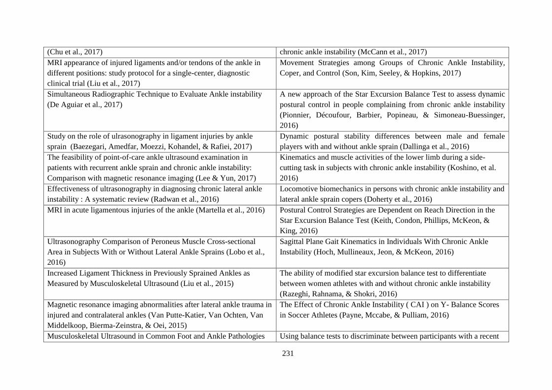
231

(Chu et al., 2017) chronic ankle instability (McCann et al., 2017)

MRI appearance of injured ligaments and/or tendons of the ankle in

different positions: study protocol for a single-center, diagnostic

clinical trial (Liu et al., 2017)

Movement Strategies among Groups of Chronic Ankle Instability,

Coper, and Control (Son, Kim, Seeley, & Hopkins, 2017)

Simultaneous Radiographic Technique to Evaluate Ankle instability

(De Aguiar et al., 2017)

A new approach of the Star Excursion Balance Test to assess dynamic

postural control in people complaining from chronic ankle instability

(Pionnier, Découfour, Barbier, Popineau, & Simoneau-Buessinger,

2016)

Study on the role of ulrasonography in ligament injuries by ankle

sprain (Baezegari, Amedfar, Moezzi, Kohandel, & Rafiei, 2017)

Dynamic postural stability differences between male and female

players with and without ankle sprain (Dallinga et al., 2016)

The feasibility of point-of-care ankle ultrasound examination in

patients with recurrent ankle sprain and chronic ankle instability:

Comparison with magnetic resonance imaging (Lee & Yun, 2017)

Kinematics and muscle activities of the lower limb during a side-

cutting task in subjects with chronic ankle instability (Koshino, et al.

2016)

Effectiveness of ultrasonography in diagnosing chronic lateral ankle

instability : A systematic review (Radwan et al., 2016)

Locomotive biomechanics in persons with chronic ankle instability and

lateral ankle sprain copers (Doherty et al., 2016)

MRI in acute ligamentous injuries of the ankle (Martella et al., 2016) Postural Control Strategies are Dependent on Reach Direction in the

Star Excursion Balance Test (Keith, Condon, Phillips, McKeon, &

King, 2016)

Ultrasonography Comparison of Peroneus Muscle Cross-sectional

Area in Subjects With or Without Lateral Ankle Sprains (Lobo et al.,

2016)

Sagittal Plane Gait Kinematics in Individuals With Chronic Ankle

Instability (Hoch, Mullineaux, Jeon, & McKeon, 2016)

Increased Ligament Thickness in Previously Sprained Ankles as

Measured by Musculoskeletal Ultrasound (Liu et al., 2015)

The ability of modified star excursion balance test to differentiate

between women athletes with and without chronic ankle instability

(Razeghi, Rahnama, & Shokri, 2016)

Magnetic resonance imaging abnormalities after lateral ankle trauma in

injured and contralateral ankles (Van Putte-Katier, Van Ochten, Van

Middelkoop, Bierma-Zeinstra, & Oei, 2015)

The Effect of Chronic Ankle Instability ( CAI ) on Y- Balance Scores

in Soccer Athletes (Payne, Mccabe, & Pulliam, 2016)

Musculoskeletal Ultrasound in Common Foot and Ankle Pathologies Using balance tests to discriminate between participants with a recent

232

(Badon & Brown, 2015) index lateral ankle sprain and healthy control participants: A cross-

sectional study (Pourkazemi et al., 2016)

Ultrasonography in the Assessment of Lateral Ankle Ligament Injury,

Instability, and Anterior Ankle Impingement: A Diagnostic Case

Report (Battaglia, Craig, & Kettner, 2015)

Ultrasound and radiography

Kinematic predictors of star excursion balance test performance in

individuals with chronic ankle instability (Hoch et al., 2016)

Ultrasound Findings of the Painful Ankle and Foot (Artul & Habib,

2014)

Laboratory Measures of Postural Control During the Star Excursion

Balance Test After Acute First-Time Lateral Ankle Sprain (Doherty et

al., 2015)

Unrecognised Acute Rupture of the Achilles Tendon in Severe Ankle

Sprain (Wai & Hing, 2015)

Individuals with both perceived ankle instability and mechanical laxity

demonstrate dynamic postural stability deficits (Brown et al., 2015)

MRI in chronic ankle inversion injures (Pashnikova, Trufanov, Fokin,

& Pchelin, 2014)

Lower Extremity Muscle Activation in Patients With or Without

Chronic Ankle Instability During Walking (Feger, Donovan, Hart, &

Hertel, 2015)

Structural abnormalities and persistent complaints after an ankle sprain

are not associated: an observational case control study in primary care

(Van Ochten et al., 2014)

Multi-segment foot landing kinematics in subjects with chronic ankle

instability (De Ridder et al., 2015)

The use of MRI in pre-operative evaluation of anterior talofibular

ligament in chronic ankle instability (Kanamoto, Shiozaki, Tanaka,

Yonetani, & Horibe, 2014)

Weight-Bearing Dorsiflexion Range of Motion and Landing

Biomechanics in Individuals With Chronic Ankle Instability (Hoch,

Farwell, Gaven, & Weinhandl, 2015)

Value of ultrasonography for detecting chronic injury of the lateral

ligaments of the ankle joint compared with ultrasonography findings

(Cheng, Cai, & Wang, 2014)

Acute Ankle Sprain Injury Alters Kinematic and Center of Pressure

Measures of Postural Control During The Star Excursion Balance Test

(Doherty et al., 2014)

Application of Ultrasound in Sports Injury (Chiang, Wang, & Hsieh,

2013)

Balance failure in single limb stance due to ankle sprain injury: An

analysis of centre of pressure using the fractal dimension method

(Doherty et al., 2014)

The accuracy of ultrasound evaluation in foot and ankle trauma

(Ekinci, Polat, Günalp, Demirkan, & Koca, 2013)

Concurrent and Discriminant Validity of the Star Excursion Balance

Test for Military Personnel With Lateral Ankle Sprain (Bastien et al.,

233

2014)

The Role of Dynamic Ultrasound and MRI in the poorly resolving

ankle sprain (Zietkiewicz, Mercouris, & Marshall, 2013)

Dynamic Postural Control Assessment with Star Excursion Balane

Test among Chronic Ankle Instability and Healthy (Khuman, Surbala,

& Kamlesh, 2014)

New method of diagnosis for chronic ankle instability: Comparison of

manual anterior drawer test, stress radiography and stress ultrasound

(Lee et al., 2013)

Postural control strategies during single limb stance following

acute lateral ankle sprain (Doherty et al., 2014b)

Ultrasound-assisted triage of ankle trauma can decrease the need for

radiographic imaging (Hedelin, Goksör, Karlsson, & Stjernström,

2013)

Postural-Stability Tests That Identify Individuals With Chronic Ankle

Instability (Linens, Ross, Arnold, Gayle, & Pidcoe, 2014)

Ultrasound examination of the ankle: most prevalent disease in our

environment (Molero et al., 2013)

Ankle dorsiflexion range of motion influences dynamic balance in

individuals with chronic ankle instability (Basnett et al., 2013)

Accuracy of MRI findings in chronic lateral ankle ligament injury

comparison with surgical finding (Park et al., 2012)

Ankle kinematics of individuals with chronic ankle instability while

walking and jogging on a treadmill in shoes (Chinn, Dicharry, &

Hertel, 2013).

Chronic ankle instability: diagnosis and treatment (Rodriguez-

Merchan, 2012)

Examining the diagnostic accuracy of dynamic postural stability

measures in differentiating among ankle instability status (Liu et al.,

2013)

Differences in Lateral Ankle Laxity Measured via Stress

Ultrasonography in Individuals With Chronic Ankle Instability, Ankle

Sprain Copers, and Healthy Individuals (Croy et al., 2012)

Using the Star Excursion Balance Test to Assess Dynamic Postural-

Control Deficits and Outcomes in Lower Extremity Injury: A

Literature and Systematic Review (Gribble, Hertel, & Plisky, 2012)

Diagnosis and treatment of acute ankle injuries: development of an

evidence-based algorithm (Polzer, 2012)

Dorsiflexion range of motion significantly influences dynamic balance

(Hoch, Staton, & McKeon, 2011).

Ultrasound examination for the diagnosis of chronic anterior

talofibular ligament injury (Hau et al., 2012)

Functional Performance Testing in Athletes with Functional Ankle

Instability (Sharma, Sharma, & Sandhu, 2011)

Accuracy of Plain Radiographs Versus 3D Analysis of Ankle Stress

Test (Hoffman et al., 2011)

Spatial postural control alterations with chronic ankle instability (Pope

et al., 2011)

Accuracy of MRI scan in the diagnosis of ligamentous and chondral The effect of EMG activity of the lower leg with dynamic balance of

234

pathology in the ankle (Joshy, Abdulkadir, Chaganti, Sullivan, &

Hariharan, 2010)

the recreational athletes with functional ankle instability (Ahn, Kim, &

Kim, 2011)

Chronic ankle instability. Which tests to assess the lesions? Which

therapeutic options? (Tourné, Besse, & Mabit, 2010)

Difference in balance measures between patients with chronic ankle

instability and patients after an acute ankle inversion trauma (de Vries,

Kingma, Blankevoort, & van Dijk, 2010)

Evaluation of anterior talofibular ligament injury with stress

radiography, ultrasonography and MR imaging (Oae, Takao, Uchio, &

Ochi, 2010)

Dynamic Postural Stability in Females with Chronic Ankle Instability

(Brown, Bowser, & Orellana, 2010)

Is MRI Adequate to Detect Lesions in Patients with Ankle Instability?

(O’Neill,‎Aman,‎&‎Guyton,‎2010)

Dynamic postural control but not mechanical stability differs among

those with and without chronic ankle instability (Wikstrom et al.,

2010)

Value of ultrasonography for detecting ligament damage in athletes

with chronic ankle instability compared to computed arthotomography

(Guillodo, Varache, & Saraux, 2010)

Postural control differs between those with and without chronic ankle

instability (Wikstrom, Fournier, & McKeon, 2010)

Ankle Ligaments on MRI Appearance of Normal and Injured

Ligaments (Perrich, Goodwin, Hecht, & Cheung, 2009)

The Effects of Fatigue and Chronic Ankle Instability on Dynamic

Postural Control (Hosseinimehr, Daneshmandi, & Norasteh, 2010).

The Value of Ultrasound in Acute Ankle Injury: Comparison With MR

(Margetic et al., 2009)

Alterations in knee kinematics and dynamic stability associated with

chronic ankle instability (Gribble & Robinson, 2009)

Audit on the use of radiography and the management of ankle sprains

in A&E (Borg & Pickard, 2008)

Functional performance deficits in patients with CAI: Validity of the

multiple hop test (Eechaute et al., 2008)

Functional Performance Testing in Participants With Functional Ankle

Instability and in a Healthy Control Group (Buchanan, Docherty, &

Schrader, 2008)

Spatiotemporal postural control deficits are present in those with

chronic ankle instability (McKeon & Hertel, 2008)

235

References

Abate, M. (2014). How obesity modifies tendons (implications for athletic activities).

Muscles, Ligaments and Tendons Journal, 4(3), 298–302.

Abate, M., Gravare-Silbernagel,‎K.,‎Siljeholm,‎C.,‎Di‎Iorio,‎A.,‎De‎Amicis,‎D.,‎Salini,‎V.,‎…‎

Paganelli, R. (2009). Pathogenesis of tendinopathies: inflammation or degeneration?

Arthritis Research & Therapy, 11(3), 1-15.

Abate, M., Schiavone, C., Di Carlo, L., & Salini, V. (2012). Achilles tendon and plantar

fascia in recently diagnosed type II diabetes: Role of body mass index. Clinical

Rheumatology, 31(7), 1109–1113.

Abdeen, R., Comfort, P., Starbuck, C., & Nester, C. (2018). Ultrasound Characteristics of

Foot and Ankle Structures in Healthy, Coper, and Chronically Unstable Ankles. Journal

of Ultrasound in Medicine, 1–10.

Agut, A., Martínez, M., Sánchez-Valverde, M., Soler, M., & Rodríguez, M. (2009).

Ultrasonographic characteristics (cross-sectional area and relative echogenicity) of the

digital flexor tendons and ligaments of the metacarpal region in Purebred Spanish

horses. Veterinary Journal, 180(3), 377–383.

Ahmed, R., & Nazarian, L. (2010). Overview of musculoskeletal sonography. Ultrasound

Quarterly, 26(1), 27–35.

Ahn, C., Kim, H., & Kim, M. (2011). The Effect of the EMG Activity of the Lower Leg with

Dynamic Balance of the Recreational Athletes. Journal of Physical Therapy Science,

23(4), 579–583.

Akbari, M., Karimi, H., Farahini, H., & Faghihzadeh, S. (2006). Balance problems after

unilateral lateral ankle sprains. The Journal of Rehabilitation Research and

Development, 43(7), 819.

Aksenov, A. (2014). An Investigation Into the Relationship Between Rocker Sole Designs and

Alteration To Lower Limb Kinetics, Kinemarics And Muscle Function During Adult

Gail. University of Salford.

Al-Mohrej, O., & Al-Kenani, N. (2016). Acute ankle sprain: conservative or surgical

approach? EFORT Open Reviews, 1(2), 28–38.

Alenezi, F. (2016). The Relationship Between Lower Limb Biomechanical Variables During

Common Screening Tasks. University of Salford.

Almansour, A. (2015). Identifying indicators of functional recovery after ankle sprain in

physically active people. Cardiff University.

Anandacoomarasamy, A., & Barnsley, L. (2005). Long term outcomes of inversion ankle

injuries. British Journal of Sports Medicine, 39(3), e14; discussion e14.

Andersen, T., Floerenes, T., Arnason, A., & Bahr, R. (2004). Video Analysis of the

Mechanisms for Ankle Injuries in Football. American Journal of Sports Medicine, 32(1),

69S–79S.

Anderson, P. (2016). Star excursion balance tests as a measure of functional joint mobility:

236

an exploratory study. Norwegian School of Sport Sciences.

Andrade, R., Mello, F., Marchiori, E., Augusto, A., Santos, S., & Neto, G.(2006).

Morphometric Evaluation of Achilles Tendon By Ultrasound. Radiologia Brasileira,

39(3), 1–10.

Angin, S., Crofts, G., Mickle, K., & Nester, C. (2014). Ultrasound evaluation of foot muscles

and plantar fascia in pes planus. Gait and Posture, 40(1), 48–52.

Apoorva, D., Lalitha, C., & Patil, G. (2014). Morphometric Study of Calcaneofibular

Ligament of Ankle. Journal of Evidence Based Med & Hlthcare, 1(10), 1268–1274.

Arnason, A., Sigurdsson, S., Gudmundsson, A., & Holme, I. (2004). Risk Factors for Injuries

in Football. American Orthopaedic Society for Sports Medicine, 32(1), 5–16.

Arnold, B., De La Motte, S., Linens, S., & Ross, S. (2009). Ankle instability is associated

with balance impairments: A meta-analysis. Medicine and Science in Sports and

Exercise, 41(5), 1048–1062.

Arnold, B., & Docherty, C. (2006). Frequency of Giving Way. Journal of Athletic Training,

41(3), 233–238.

Arts, I., Pillen, S., Schelhaas, H., Overeem, S., & Zwarts, M. (2010). Normal values for

quantitative muscle ultrasonography in adults. Muscle and Nerve, 41(1), 32–41.

Arts,‎I.,‎Schelhaas,‎H.,‎Verrijp,‎K.,‎Zwarts,‎M.,‎Overeem,‎S.,‎van‎der‎Laak,‎J.,‎…‎Pillen, S.

(2012). Intramuscular fibrous tissue determines muscle echo intensity in amyotrophic

lateral sclerosis. Muscle and Nerve, 45(3), 449–450.

Artul, S., & Habib, G. (2014). Ultrasound findings of the painful ankle and foot. Journal of

Clinical Imaging Science, 4(2), 25.

Ashton-Miller, J., Ottaviani, R., Hutchinson, C., & Wojtys, E. (1996). What best protects the

inverted weightbearing ankle against further inversion?: Evertor Muscle Strength

Compares Favorably with Shoe Height, Athletic Tape, and Three Orthoses. American

Journal of Sports Medicine, 24(6), 800–809.

Aslan, A., Sofu, H., & Kirdemir, V. (2014). Ankle Ligament Injury: current concept. OA

Orthopaedics, 2(1).

Asplund, C., & Best, T. (2013). Achilles tendon disorders. British Medical Journal, 346, 29–

33.

Attarian, D., McCrackin, H., Devito, D., McElhaney, J., & Garrett, W. (1985). A

biomechanical study of human lateral ankle ligaments and autogenous reconstrustive

grafts. American Journal of Sports Medicine, 13(6), 377–381.

Audenaert, A., Prims, J., Reniers, G., Weyns, D., Mahieu, P., & Audenaert, E. (2010).

Evaluation and economic impact analysis of different treatment options for ankle

distortions in occupational accidents. Journal of Evaluation in Clinical Practice, 16(5),

933–939.

Bachmann, L., Kolb, E., Koller, M., Steurer, J., & Riet, G. (2003). Accuracy of Ottawa ankle

rules to exclude fractures of the ankle and Mid-Foot :‎ Systematic‎ Review.‎ British

237

Medical Journal, 36, 1–7.

Backhaus, M., Ohrndorf, S., Naumann, L., Grundey, J., Scheel, T., Scheel, A., & Werner, C.

(2010). Is musculoskeletal ultrasonography an operator-dependent method or a fast and

reliably teachable diagnostic tool? Interreader agreements of three ultrasonographers

with different training levels. International Journal of Rheumatology, 2010.

Backman, L., & Danielson, P. (2011). Low range of ankle dorsiflexion predisposes for

patellar tendinopathy in junior elite basketball players: A 1-year prospective study.

American Journal of Sports Medicine, 39(12), 2626–2633

Basnett, C., Hanish, M., Wheeler, T., Miriovsky, D., Danielson, E., Barr, J., & Grindstaff, T.

(2013). Ankle dorsiflexion range of motion influences dynamic balance in individuals

with chronic ankle instability. International Journal of Sports Physical Therapy, 8(2),

121–8

Baezegari, H., Amedfar, A., Moezzi, M., Kohandel, S., & Rafiei, A. (2017). Study on the

Role of Ultrasonography in Ligament Injuries By Ankle Sprain. International Journal

Life Science & Pharma Research, 7(1), 29–36.

Balakrishnan, N. (2014). Methods and Applications of Statistics in Clinical Trials. Methods

and Applications of Statistics in Clinical Trials (Vol. 2).

Bartlett, R., & Bussey, M. (2012). Sport biomechanics: reducing injury risk and improving

sports performance. New York: Taylor & Francis Ltd - M.U.A.

Basnett, C., Hanish, M., Wheeler, T., Miriovsky, D., Danielson, E., Barr, J., & Grindstaff, T.

(2013). Ankle dorsiflexion range of motion influences dynamic balance in individuals

with chronic ankle instability. International Journal of Sports Physical Therapy, 8(2),

121–128.

Bass, C., & Marriott, P. (2009). Ultrasound of the ankle. Australian Journal of Ultrasound in

Medicine, 12(November), 10–17.

Baumhauer, J., Alosa, D., Renström, P., Trevino, S., & Beynnon, B. (1995). A Prospective

Study of Ankle Injury Risk Factors. The American Journal of Sports Medicine, 23(5),

564–570.

Bautista, D. (2016). Effective use of Pilot studies. Clinical Research for the Nation. Retrieved

from https://www.scri.edu.sg/wp-content/uploads/2016/10/Effective-use-of-Pilot-

studies_final-DB.pdf

Beazell, J., Grindstaff, T., Sauer, L., Magrum, E., Ingersoll, C., & Hertel, J. (2012). Effects of

a Proximal or Distal Tibiofibular Joint Manipulation on Ankle Range of Motion and

Functional Outcomes in Individuals With Chronic Ankle Instability. Journal of

Orthopaedic & Sports Physical Therapy, 42(2), 125–134.

Berben, L., Sereika, S., & Engberg, S. (2012). Effect size estimation: Methods and examples.

International Journal of Nursing Studies, 49(8), 1039–1047.

Bernier, J., Perrin, D., & Rijke, A. (1997). Effect of unilateral functional instability of the

ankle on postural sway and inversion and eversion strength. Journal of Athletic

238

Training, 32, 226–232.

Beynnon,‎B.,‎Renstrom,‎P.,‎Alosa,‎D.,‎Baumhauer,‎J.,‎Vacek,‎P.,‎Surgery,‎O.,‎…‎Uniaersity,‎

S.‎ (2001).‎Ankle‎ ligament‎ injury‎ risk‎ factors :‎ a‎ prospective‎ study‎ of‎ college‎ athletes.‎

Journal of Orthopaedic Research, 19, 213–220.

Bisschops, J., & Lavallee, M. (2016). Anatomy of the Leg. In Muscular Injuries in the

Posterior Leg Assessment and Treatment. Springer.

Bjordal, J., Demmink, J., & Ljunggren, A. (2003). Tendon thickness and depth from skin for

supraspinatus, common wrist and finger extensors, patellar and achilles tendons:

Ultrasonography study of healthy subjects. Physiotherapy, 89(6), 375–383.

Black, J., Cook, J., Kiss, Z., & Smith, M. (2004). Intertester reliability of sonography in

patellar tendinopathy. Journal‎ of‎ Ultrasound‎ in‎ Medicine :‎ Official Journal of the

American Institute of Ultrasound in Medicine, 23(5), 671–5.

Bland, J., & Altman, D. (1986). Statistical methods for assessing agreement between two

methods of clinical measurement. Lancet.

Blessing, J., & Forrister, J. (2015). Introduction to research and medical literature for health

professionals. Jones & Bartlett Publishers.

Bonnel, F., Toullec, E., Mabit, C., & Tournne, Y. (2010). Chronic ankle instability:

Biomechanics and pathomechanics of ligaments injury and associated lesions.

Orthopaedics and Traumatology: Surgery and Research, 96(4), 424–432.

Braun, B. (1999). Effects of ankle sprain in a general clinic population 6 to 18 months after

medical evaluation. Archives of Family Medicine, 8(2), 143–148.

Bridgman, S., Clement, D., Wallety, G., Phair, I., & Maffulli, N. (2003). Population based

epidemiology of ankle sprains attending accident and emergency units in the West

Midlands of England, and a survey of UK practice for severe ankle sprains. Emergency

Medicine Journal, 20(6), 508–510.

Brockett, C., & Chapman, G. (2016). Biomechanics of the ankle. Orthopaedics and Trauma,

30(3), 232–238.

Brown, C., Bowser, B., & Orellana, A. (2010). Dynamic postural stability in females with

chronic ankle instability. Medicine and Science in Sports and Exercise, 42(12), 2258–

2263.

Brown, C., & Mynark, R. (2007). Balance Deficits in Recreational Athletes With Chronic

Ankle Instability. Journal of Athletic Training, 42(3), 367–373.

Brown, C., Padua, D., Marshall, S., & Guskiewicz, K. (2011). Hip Kinematics During a Stop-

Jump Task in Patients With Chronic Ankle Instability. Journal of Athletic Training,

46(5), 461–470.

Brown, C., Ross, S., Mynark, R., & Guskiewicz, K. (2004). Assessing Functional Ankle

Instability With Joint Position Sense, Time to Stabilization, and Electromyography.

Journal Sport Rehabilitation, 13, 122–134.

Bruton, A., Conway, J., & Holgate, S. (2000). Reliability: What is it, and how is it measured?

239

Physiotherapy, 86(2), 94–99.

Buchanan, A., Docherty, C., & Schrader, J. (2008). Functional performance testing in

participants with functional ankle instability and in a Healthy Control Group. Journal of

Athletic Training, 43(4), 342–346.

Buschmann, J., & Burgisser, G. (2017). Biomechanics of Tendon and Ligament: Tissue

Reconstruction and Regeneration. Elsevier Ltd.

Cadore, E., Izquierdo, M., Conceição,‎M.,‎Radaelli,‎R.,‎Pinto,‎R.,‎Baroni,‎B.,‎…‎Kruel,‎L.

(2012). Echo intensity is associated with skeletal muscle power and cardiovascular

performance in elderly men. Experimental Gerontology, 47(6), 473–478.

Cai, Y., Li, S., Chen, S., Hua, Y., & Shan, J. (2017). An Ultrasound Classification of Anterior

Talofibular Ligament ( ATFL ) Injury. The Open Orthopaedics Journal, (11), 610–616.

Cameron, K., Owens, B., & Deberardino, T. (2010). Incidence of ankle sprains among active-

duty members of the united states armed services from 1998 through 2006. Journal of


Campbell, S. E. (2006). MRI of Sports Injuries of the Ankle. Clinics in Sports Medicine,

25(4), 727–762.

Cao, S., Wang, C., Ma, X., Wang, X., Huang, J., & Zhang, C. (2018). Imaging diagnosis for

chronic lateral ankle ligament‎injury :‎a‎systemic‎review‎with‎meta-analysis. Journal of

Orthopaedic Surgery and Research, 1–14.

Caplan, N., & Kader, D. (2014). Rating Systems in the Evaluation of Knee Ligament Injuries.

In Classic Papers in Orthopaedics (pp. 201–203). Springer Science & Business Media.

Cappozzo, A., Catani, F., Della Croce, U., & Leardini, A. (1995). Position and orietnation in

space of bones during movement. Clinical Biomechanics, 10(4), 171–178.

Carovac, A., Smajlovic, F., & Junuzovic, D. (2011). Application of Ultrasound in Medicine.

Acta Inform Med, 19(3), 168–171.

Caulfield, B., Crammond, T., Sullivan, A., Reynolds, S., & Ward, T. (2004). Altered Ankle-

Muscle Activation During Jump Landing in Participants With Functional Instability of

the Ankle Joint. Journal Sport Rehabilitation, 13, 189–201.

Caulfield, B., & Garrett, M. (2004). Changes in ground reaction force during jump landing in

subjects with functional instability of the ankle joint. Clinical Biomechanics, 21, 168–

174.

Caulfield, B., & Garrett, M. (2002). Functional instability of the ankle: Differences in

patterns of ankle and knee movement prior to and post landing in a single leg jump.

International Journal of Sports Medicine, 23(1), 64–68.

Çekiç, B., Mutlu, I., Parlak, A.,‎Köksel,‎Y.,‎Erdem‎Toslak,‎İ.,‎&‎Parlak,‎M.‎(2017).‎B-Mode

Gray Scale Histogram Value in Diagnosis of Adolescent Patients with Hashimoto

Thyroiditis. İstanbul‎Medical‎Journal, 18, 222–6.

Chae, S., Kim, Y., & Lee, S. (2017). Effects of phase proprioceptive training on balance in

patients with chronic stroke. Journal of Physical Therapy Science, 29(5), 839–844.

240

Chan, K., Ha, S., Fong, D., & Chan, K. (2014). Analysis of ankle inversion sprain injury

mechanism from accidental injury cases captured in televised basketball matches.

Journal of Foot and Ankle Research,7,1-2 .

Chan, V., & Perlas, A. (2011). Basics of Ultrasound Imaging. In Atlas of ultrasound-guided

procedures in interventional pain management (pp. 13–19). Springer Scince.

Chan, Y., Fong, D., Yung, P., Fung, K., & Chan, K. (2008). A mechanical supination sprain

simulator for studying ankle supination sprain kinematics. Journal of Biomechanics,

41(11), 2571–4.

Cheng, J., Tsai, W., Yu, T., & Huang, K. (2012). Reproducibility of sonographic

measurement of thickness and echogenicity of the plantar fascia. Journal of Clinical

Ultrasound, 40(1), 14–19.

Cheng, Y., Cai, Y., & Wang, Y. (2014). Value of ultrasonography for detecting chronic

injury of the lateral ligaments of the ankle joint compared with ultrasonography

findings. British Journal of Radiology, 87,1-6.

Cheuvront, S. N., Moffatt, R. J., & DeRuisseau, K. C. (2016). Body composition and gender

differences in performance. In Second (Ed.), Nutritional Assessment of Athletes (pp.

121–148). CRC Press.

Cho, K., Lee, K., Lee, B., Lee, H., & Lee, W. (2014). Relationship between Postural Sway

and Dynamic Balance in Stroke Patients. Journal of Physical Therapy Science, 26(12),

1989–1992.

Cho, K., & Wansaicheong, G. (2012). Ultrasound of the foot and ankle. Ultrasound Clinics,

7(4), 487–503.

Choi, W., Lee, J., & Han, S. (2008). Chronic Lateral Ankle Instability:The Effect of Intra-

Articular Lesions. The American Journal of Sports Medicine, 36(11), 2167–2172.

Chou, S., Chen, C., Su, H., Hsu, M., Liang, S., & Hsu, C. (2011). Ultrasonographic

quantification of the endometrium during the menstrual cycle using computer-assisted

analysis. Taiwanese Journal of Obstetrics and Gynecology, 50(3), 297–300.

Chow, R., Medri, M., Martin, D., Leekam, R., Agur, A., & McKee, N. (2000). Sonographic

studies of human soleus and gastrocnemius muscle architecture: gender variability.

European Journal of Applied Physiology, 82, 236–244.

Chu, P., Chan, W., Lee, H., Hon, Y., Chan, J., & Lo, K. (2017). Magnetic Resonance

Imaging of Ligamentous Injuries in Ankle Sprain. Hong Kong Journal of Radiology, 20,

17–27.

Clark, V., & Burden, A. (2005). A 4-week wobble board exercise programme improved

muscle onset latency and perceived stability in individuals with a functionally unstable

ankle. Physical Therapy in Sport, 6(4), 181–187.

Clark, N., Treleaven, J., & Ulrik, R. (2015). Proprioception in musculoskeletal rehabilitation .

Part‎ 1 :‎Basic‎ science and principles of assessment and clinical interventions. Manual

Therapy, 20, 368–377.

Cnyrim,‎C.,‎Mergner,‎T.‎and‎Maurer,‎C.‎(2009)‎‘Potential‎roles‎of‎force‎cues‎in‎human‎stance‎

241

control’,‎Experimental Brain Research, 194(3), 419–433

Coe, R. (2004). Issues arising from the use of effect sizes in analyzing and reporting research.

In But‎what‎does‎it‎mean ?‎the‎use‎of‎effect‎sizes‎ in‎educational‎research (pp. 80–95).

National Foundation for Educational Research.

Collins, N., Teys, P., & Vicenzino,‎B.‎(2004).‎The‎initial‎effects‎of‎a‎Mulligan’s‎mobilization‎

with movement technique on dorsiflexion and pain in subacute ankle sprains. Manual

Therapy, 9(2), 77–82.

Colville, M., Marder, R., Boyle, J., & Zarins, B. (1990). Strain measurement in lateral ankle

ligaments. The American Journal of Sports Medicine, 18(2), 196–200.

Cooke, M., Lamb, S., Marsh, J., & Dale, J. (2003). A survey of current consultant practice of

treatment of severe ankle sprains in emergency departments in the United Kingdom.

Emerg Med J, 20(6), 505–507.

Cooperberg, P., Tsang, I., Truelove, L., & Knickerbocker, J. (1978). Gray Scale Ultrasound

in the Evaluation of Rheumatoid Arthritis of the Knee. Radiology, 126(3).

Coughlan, G., Fullam, K., Delahunt, E., Gissane, C., & Caulfield, B. (2012). A comparison

between performance on selected directions of the star excursion balance test and the Y

balance test. Journal of Athletic Training, 47(4), 366–371.

Crane, M. (2011). Severe Peroneal Tendon Injury Diagnosed as an Ankle Sprain. Retrieved

from http://www.myrundoc.com/permalink/Tags/tendonosis/default.aspx

Crawford, R., Walley, G., Bridgman, S., & Maffulli, N. (2007). Magnetic resonance imaging

versus arthroscopy in the diagnosis of knee pathology, concentrating on meniscal lesions

and ACL tears: A systematic review. British Medical Bulletin, 84(1), 5–23.

Crofts, G., Angin, S., Mickle, K., Hill, S., & Nester, C. (2014). Reliability of ultrasound for

measurement of selected foot structures. Gait and Posture, 39(1), 35–39.

Croy, T., Saliba, S., Saliba, E., Anderson, M., & Hertel, J. (2012). Differences in lateral ankle

laxity measured via stress ultrasonography in individuals with chronic ankle instability,

ankle sprain copers, and healthy individuals. The Journal of Orthopaedic and Sports

Physical Therapy, 42(7), 593–600.

Croy, T., Saliba, S., Saliba, E., Anderson W., M., & Hertel, J. (2013). Talofibular Interval

Changes After Acute Ankle Sprain: A Stress Ultrasonography Study of Ankle Laxity.

Journal of Sport Rehabilitation, 22(4), 257–263.

Daftary, A., & Adler, R. (2009). Sonographic evaluation and ultrasound-guided therapy of

the Achilles tendon. Ultrasound Quarterly, 25(3), 103–110.

Dallinga, J., van der Does, H., Benjaminse, A., & Lemmink, K. (2016). Dynamic postural

stability differences between male and female players with and without ankle sprain.

Physical Therapy in Sport, 17, 69–75.

Das, S. (2016). Bedside Ultrasound of the Abdomen- Part 1. Current Med Issues, 14(4), 113–

120.

Daugherty, K., Manske, R. C., & Brotzman, S. B. (2011). Clinical Orthopaedic

242

Rehabilitation :‎An‎Evidence-based Approach (3rd ed.). Philadelphia, PA: Mosby.

Davids, K., Glazier, P., Araújo, D., & Bartlett, R. (2003). Movement systems as dynamical

systems: The functional role of variability and its implications for sports medicine.

Sports Medicine, 33(4), 245–260.

Dayakidis, M., & Boudolos, K. (2006). Ground reaction force data in functional ankle

instability during two cutting movements. Clinical Biomechanics, 21(4), 405–411.

De Asla, R., Kozánek, M., Wan, L., Rubash, H., & Li, G. (2009). Function of anterior

talofibular and calcaneofibular ligaments during in-vivo motion of the ankle joint

complex. Journal of Orthopaedic Surgery and Research, 4, 1–6.

De La Motte, S., Arnold, B. L., & Ross, S. (2015). Trunk-rotation differences at maximal

reach of the Star Excursion Balance Test in participants with chronic ankle instability.

Journal of Athletic Training, 50(4), 358–365.

De Maeseneer, M., Marcelis, S., Jager, T., Shahabpour, M., Van Roy, P., Weaver, J., &

Jacobson, J. (2009). Sonography of the normal ankle: A target approach using skeletal

reference points. American Journal of Roentgenology, 192(2), 487–495.

De Noronha, M., França, L., Haupenthal, A., & Nunes, G. (2013). Intrinsic predictive factors

for ankle sprain in active‎ university‎ students :‎ A‎ prospective‎ study.‎ Scandinavian

Journal of Medicine and Science in Sports, 23(5), 541–547.

De Noronha, M., Refshauge, K., Herbert, R., Kilbreath, S., & Hertel, J. (2006). Do voluntary

strength, proprioception, range of motion, or postural sway predict occurrence of lateral

ankle sprain?. British Journal of Sports Medicine, 40(10), 824–828.

De Noronha, M., Refshauge, K., Kilbreath, S., & Crosbie, J. (2007). Loss of proprioception

or motor control is not related to functional ankle instability: an observational study. The

Australian Journal of Physiotherapy, 53(3), 193–198.

De Ridder, R., Willems, T., Vanrenterghem, J., Robinson, M., & Roosen, P. (2015). Lower

limb landing biomechanics in subjects with chronic ankle instability. Medicine and

Science in Sports and Exercise, 47(6), 1225–1231.

De Vaus, D. (2001). Research Design in Social Research. London: SAGE.

De Vries, J., Kingma, I., Blankevoort, L., & van Dijk, C. (2010). Difference in balance

measures between patients with chronic ankle instability and patients after an acute

ankle inversion trauma. Knee Surgery, Sports Traumatology, Arthroscopy, 18(5), 601–

606.

De Wilde, J., Rensburg, J., Grant, C., & Rensburg, J. (2014). The assessment and

management of lateral ankle ligament injuries. South African Family Practice, 56(4),

13–18.

Delahunt, E., Chawke, M., Kelleher, J., Murphy, K., Prendiville, A., Sweeny, L., & Patterson,

M. (2013). Lower limb kinematics and dynamic postural stability in anterior cruciate

ligament-reconstructed female athletes. Journal of Athletic Training, 48(2), 172–185.

Delahunt, E., Coughlan, G., Caulfield, B., Nightingale, E., Lin, C., & Hiller, C. (2010).

Inclusion criteria when investigating insufficiencies in chronic ankle instability.

243

Medicine and Science in Sports and Exercise, 42(11), 2106–2121.

Delahunt, E., Monaghan, K., & Caulfield, B. (2006). Changes in lower limb kinematics,

kinetics, and muscle activity in subjects with functional instability of the ankle joint

during a single leg drop jump. Journal of Orthopaedic Res, 24(10), 1991–2000.

Delahunt, E., Monaghan, K., & Caulfield, B. (2007). Ankle function during hopping in

subjects with functional instability of the ankle joint. Scandinavian Journal of Medicine

and Science in Sports, 17(6), 641–648.

Demase, B. (2016). Medial Ankle Sprains. Retrieved from

http://physioaustraliaonline.com/ankle-pain/medial-ankle-sprain/

Demeritt, K., Shultz, S., Docherty, C., Gansneder, B., & Perrin, D. (2002). Chronic Ankle

Instability Does Not Affect Lower Extremity Functional Performance. Journal of


Demetracopulos, C., & Deland, J. (2013). Anatomy and Biomechanics of The Foot and

Ankle. In Foot and Ankle (pp. 1–23). Philadelphia, PA: Wolters Kluwer, Lippincott

Williams & Wilkins Health.

Denegar, C., & Miller, S. (2002). Can chronic ankle instability be prevented? Rethinking

management of lateral ankle sprains. Journal of Athletic Training, 37(4), 430–435.

Diaz, J., Paya, J., Ferrando, A., & Aledo, E. (2015). Medical Image Processinf, Analysis and

Visualization With Musculoskeletal Ultrasound. In Advanced Techniques in

Musculoskeletal Medicine & Physiotherapy: Using Minimally Invasive Therapies in

Practice (pp. 473–488). Elsevier Health Sciences.

DiDomenico, L., & Anania, M. (2013). Peroneal Tendon Disorders. In Mcglamry’s‎

comprehensive textbook of foot and ankle surgery (fourth, Vol. 1, pp. 1165–1180).

Wolters Kluwer, Lippincott Williams & Wilkins.

Dillehay, G., Deschler, T., Rogers, L., Neiman, H., & Hendrix, R. (1984). The

ultrasonographic characterization of tendons. Investigative Radiology, 19(4), 338–341.

Dimmick, S., Kennedy, D., & Daunt, N. (2009). Evaluation of thickness and appearance of

anterior talofibular and calcaneofibular ligaments in normal versus abnormal ankles with

MRI. Journal of Medical Imaging and Radiation Oncology, 52(6), 559–563.

Docherty, C., Gansneder, B., Arnold, B., & Hurwitz, S. (2006). Development and reliability

of the ankle instability instrument. Journal of Athletic Training, 41(2), 154–158.

Docherty, C., Valovich McLeod, T., & Shultz, S. (2006). Postural Control Deficits in

Participants with Functional Ankle Instability as Measured by the BESS. Clinical

Journal of Sport Medicine, 16(3), 19–21.

Doherty, C., Bleakley, C., Delahunt, E., & Holden, S. (2017). Treatment and prevention of

acute and recurrent ankle sprain: an overview of systematic reviews with meta-analysis.

British Journal of Sports Medicine, 51(2), 113–125.

Doherty, C., Bleakley, C., Hertel, J., Caulfield, B., Ryan, J., & Delahunt, E. (2015a).

Dynamic Balance Deficits 6 Months Following First-Time Acute Lateral Ankle Sprain:

A Laboratory Analysis. Journal of Orthopaedic & Sports Physical Therapy, 45(8), 626–

244

633.

Doherty, C., Bleakley, C., Hertel, J., Caulfield, B., Ryan, J., & Delahunt, E. (2015b).

Laboratory Measures of Postural Control During the Star Excursion Balance Test After

Acute First-Time Lateral Ankle Sprain. Journal of Athletic Training, 50(6), 651–664.

Doherty, C., Bleakley, C., Hertel, J., Caulfield, B., Ryan, J., & Delahunt, E. (2016). Dynamic

balance deficits in individuals with chronic ankle instability compared to ankle sprain

copers 1 year after a first-time lateral ankle sprain injury. Knee Surgery, Sports

Traumatology, Arthroscopy, 24(4), 1086–1095.

Doherty, C., Delahunt, E., Caulfield, B., Hertel, J., Ryan, J., & Bleakley, C. (2014). The

Incidence‎ and‎ Prevalence‎ of‎ Ankle‎ Sprain‎ Injury :‎ A‎ Systematic‎ Review‎ and‎ Meta-

Analysis of Prospective Epidemiological Studies. Sports Medicine, 44(1), 123–140.

Donahue, M., Simon, J., & Docherty, C. (2011). Critical Review of Self-Reported Functional

Ankle Instability Measures. Foot & Ankle International, 32(12), 1140–1146.

Donahue, M., Simon, J., & Docherty, C. (2012). Reliability and Validity of a New

Questionnaire Created to Establish the Presence of Functional Ankle Instability: The

IdFAI. Athletic Training & Sports Health Care, 5(1), 38–43.

Dong, Q., & Fessell, D. (2009). Achilles tendon ultrasound technique. American Journal of

Roentgenology, 193(3), 2009.

Doral, M., Alam, M., Bozkurt, M., Turhan, E., Atay, O. A., Dönmez, G., & Maffulli, N.

(2010). Functional anatomy of the Achilles tendon. Knee Surgery, Sports Traumatology,

Arthroscopy, 18(5), 638–643.

Doody, O., & Doody, C. (2015). Conducting a pilot study: case study of a novice researcher.

British Journal of Nursing, 24(21), 1074–1078.

Drewes, L., McKeon, P., Kerrigan, C., & Hertel, J. (2009). Dorsiflexion deficit during

jogging with chronic ankle instability. Journal of Science and Medicine in Sport, 12(6),

685–687.

Drolet, P., Martineau, A., Lacroix, R., & Roy, J. (2016). Reliability of ultrasound evaluation

of the long head of the biceps tendon. J Rehabil Med, 48(6), 554–558.

Dubin, J., Comeau, D., McClelland, R., Dubin, R., & Ferrel, E. (2011). Lateral and

syndesmotic ankle sprain injuries: a narrative literature review. Journal of Chiropractic

Medicine, 10(3), 204–19.

Dundas, M., Gutierrez, G., & Pozzi, F. (2014). Neuromuscular control during stepping down

in continuous gait in individuals with and without ankle instability. Journal of Sports

Sciences, 32(10), 926–933.

Earl, J., & Hertel, J. (2001). Lower-extremity muscle activation during the star excursion

balance tests. Journal of Sport Rehabilitation, 10, 93–104.

Edwards, M. (2017). The Planes of Motion Explained. [Blog post]. Retrieved from

https://www.acefitness.org/fitness-certifications/resource-center/exam-preparation-

blog/2863/the-planes-of-motion-explained?topicScope=exercise-science

Eechaute, C., Vaes, P., & Duquet, W. (2008a). Functional performance deficits in patients

245

with CAI: Validity of the multiple hop test. Clinical Journal of Sport Medicine, 18(2),

124–129.

Eechaute, C., Vaes, P., & Duquet, W. (2008b). The chronic ankle instability scale:

Clinimetric properties of a multidimensional, patient-assessed instrument. Physical

Therapy in Sport, 9(2), 57–66.

Eils, E., & Rosenbaum, D. (2001). A multi-station proprioceptive exercise program in

patients with ankle instability. Medicine & Science in Sports & Exercise, 33(12), 1991–

1998.

Ekinci, S., Polat, O., Günalp, M., Demirkan, A., & Koca, A. (2013). The accuracy of

ultrasound evaluation in foot and ankle trauma. The American Journal of Emergency

Medicine, 31(11), 1551–1555.

El-Liethy, N., & Kamal, H. (2016). High resolution ultrasonography and magnetic resonance

imaging in the evaluation of tendino-ligamentous injuries around ankle joint. Egyptian

Journal of Radiology and Nuclear Medicine, 47(2), 543–555.

Elliot, D., & Giesen, T. (2013). Primary Flexor Tendon Surgery. The Search for a Perfect

Result. Hand Clinics.

Engebretsen, A., Myklebust, G., Holme, I., Engebretsen, L., & Bahr, R. (2009). Intrinsic risk

factors for acute ankle injuries among male soccer players: A prospective cohort study.

Scandinavian Journal of Medicine and Science in Sports, 20(3), 403–410.

Erol,‎ B.,‎ Kara,‎ T.,‎ Gürses,‎ C.,‎ Karakoyun,‎ R.,‎ Köroǧlu,‎ M.,‎ Süren,‎ D.,‎ &‎ Bülbüller,‎ N.‎

(2013). Gray scale histogram analysis of solid breast lesions with ultrasonography: Can

lesion echogenicity ratio be used to differentiate the malignancy? Clinical Imaging,

37(5), 871–875.

Fallat, L., Grimm, D., & Saracco, J. (1998). Sprained ankle syndrome: prevalence and

analysis of 639 acute injuries. The Journal of Foot and Ankle Surgery, 37(4), 280–285.

Farr, B., Naguyen, D., Stephenson, K., Rogers, T., Stevens, F., & Jasko, J. (2017). Ankle

Sprains. In Clinical Orthopaedic Rehabilitation: a Team Approach (Fourth Edi, pp.

255–272). Elsevier Health Sciences.

Feger, M., Donovan, L., Hart, J., & Hertel, J. (2014). Lower Extremity Muscle Activation

During Functional Exercises in Patients With and Without Chronic Ankle Instability.

PM and R, 6(7), 602–611.

Fessell, D., & Jacobson, J. (2009). Ultrasound of the Hindfoot and Midfoot. Ultrasound

Clinics, 4(6), 237–253.

Fisher, R. (1954). Statistical methods for research workers. Edinburgh: Oliver and Boyd.

Fitzgordon, J. (2017). Weak Inner Thighs And The Peroneal Muscles. Retrieved from

https://corewalking.com/weak-inner-thighs-and-the-peroneal-muscles/

Fong, D., Chan, Y., Mok, K., Yung, P., & Chan, K. (2009a). Understanding acute ankle

ligamentous sprain injury in sports. Sports Medicine, Arthroscopy, Rehabilitation,

Therapy & Technology, 1(1), 14.

246

Fong, D., Chung, M., Chan, Y., Chan, K. (2012). A mechanical jig for measuring ankle

supination and pronation torque in vitro and in vivo. Medical Engineering & Physics,

34, 791-794.

Fong, D., Ha, S., Mok, K., Chan, C., & Chan, K. (2012). Kinematics Analysis of Ankle

Inversion Ligamentous Sprain Injuries in Sports: Five Cases From Televised Tennis

Competitions. The American Journal of Sports Medicine, 40(11), 2627–2632.

Fong, D., Hong, Y., Chan, L., Yung, P., & Chan, K. (2007). A Systematic Review on Ankle

Injury and Ankle Sprain in Sports. Sports Medicine, 37(1), 73–94.

Fong, D., Hong, Y., Shima, Y., Krosshaug, T., Yung, P., & Chan, K. (2009b). Biomechanics

of supination ankle sprain: a case report of an accidental injury event in the laboratory.

The American Journal of Sports Medicine, 37(4), 822–827.

Fong, D., Lam, M., Lai, P., Yung, P., Fung, K., & Chan, K. (2014). Effect of anticipation on

knee kinematics during a stop-jump task. Gait & Posture, 39(1), 75–79.

Fong, D., Man, C., Yung, P., Cheung, S., & Chan, K. (2008). Sport-related ankle injuries

attending an accident and emergency department. Injury, 39(10), 1222–1227.

Fong, D., Wang, D., Chu, V., & Chan, K. (2013). Myoelectric stimulation on peroneal

muscles with electrodes of the muscle belly size attached to the upper shank gives the

best effect in resisting simulated ankle sprain motion. Journal of Biomechanics, 46(6),

1088–1091.

Fong, D., Wei, F., Hong, Y., Krosshaug, T., Haut, R.,‎ Chan,‎ K.,‎…‎ Stadion,‎ U.‎ (2011).‎

ANKLE LIGAMENT STRAIN DURING SUPINATION SPRAIN INJURY – A

COMPUTATIONAL BIOMECHANICS STUDY. Portuguese Journal of Sport

Sciences, 11, 655–658.

Ford, K., Myer, G., & Hewett, T. (2003). Valgus Knee Motion during Landing in High

School Female and Male Basketball Players. Med Sci Sports Exerc, 35(10), 1745–1750.

Fousekis, K., Tsepis, E., & Vagenas, G. (2012). Intrinsic Risk Factors of Noncontact Ankle

Sprains in Soccer: A Prospective Study on 100 Professional Players. The American


Fox, A., Bedi, A., & Rodeo, S. (2009). The basic science of articular cartilage: Structure,

composition, and function. Sports Health, 1(6), 461–468.

Frank, C. (2004). Ligament structure, physiology and function. Journal of Musculoskeletal &

Neuronal Interactions, 4(2), 199–201.

Fredberg, U., Bolving, L., Andersen, N., & Stengaard-Pedersen, K. (2008). Ultrasonography

in Evaluation of Achilles and Patella Tendon Thickness. Ultrascall in Der Medizin, 29,

60–65.

Freeman, M. (1965). Instability of the foot after injuries to the lateral ligament of the ankle.

The Journal of Bone and Joint Surgery British Edition, 47(4), 669–77.

Fu, W., Fang, Y., Liu, Y., & Hou, J. (2014). The effect of high-top and low-top shoes on

ankle inversion kinematics and muscle activation in landing on a tilted surface. Journal

of Foot and Ankle Research, 7(1), 14.

247

Fujiwara,‎K.,‎Asai,‎H.,‎ Toyama,‎H.,‎Kunita,‎K.,‎Yaguchi,‎C.,‎Kiyota,‎N.,‎…‎ Jacobs,‎ J.‎V.‎

(2010). Changes in muscle thickness of gastrocnemius and soleus associated with age

and sex. Aging Clinical and Experimental Research, 22(1), 24–30.

Fullam, K., Caulfield, B., Coughlan, G., & Delahunt, E. (2014). Kinematic Analysis of

Selected Reach Directions of the Star Excursion Balance Test Compared with the Y-

Balance Test. Journal of Sport Rehabilitation, 23(1), 27–35.

Funk, J. (2011). Ankle injury mechanisms: Lessons learned from cadaveric studies. Clinical

Anatomy, 24(3), 350–361.

Gabriner, M., Houston, M., Kirby, J., & Hoch, M. (2015). Contributing factors to Star

Excursion Balance Test performance in individuals with chronic ankle instability. Gait

and Posture, 41(4), 912–916.

Gardner, G., Gardner, A., MacLellan, L., & Osbornea, S (2003). Reconceptualising the

objectives of a pilot study for clinical. Interanational Journal of Nursing Studie, 40(7),

719–724.

Garrick, J. (1977). The frequency of injury, mechanism of injury, and epidemiology of ankle

sprains. The American Journal of Sports Medicine, 5(6), 241–242.

Gehring, D., Wissler, S., Mornieux, G., & Gollhofer, A. (2013). How to sprain your ankle – a

biomechanical case report of an inversion trauma. Journal of Biomechanics, 46(1), 175–

178.

Gerber, J., Williams, G., Scoville, C., Arciero, R., & Taylor, D. (1998). Persistent disability

associated with ankle sprains: A prospective examination of an athletic population. Foot

and Ankle International, 19(10), 653–660.

Ghasemi, A., & Zahediasl, S. (2012). Normality Tests for Statistical Analysis: A Guide for

Non-Statisticians. International Journal of Endocrinology & Metabolism, 10(2), 486–

489.

Ghom, A. (2014). Basic Oral Radiology. JP Medical Ltd. Retrieved from

https://books.google.com/books?id=0RtPBQAAQBAJ&pgis=1

Giannone, K. (2016). Ankle Sprains. Retrieved from

http://emedicine.medscape.com/article/1907229

Giavarina, D. (2015). Understanding Bland Altman analysis. Biochemia Medica, 25(2), 141–

151.

Gill, R. (2012). The Physics and Technology of Diagnostic Ultrasound: A Practitioner’s‎

Guide. High Frequency Publishing.

Goble, D. (2010). Proprioceptive acuity assessment via joint position matching: from basic

science to general practice. Physical Therapy, 90(8), 1176–1184.

Golanó, P., Vega, J., de Leeuw, P., Malagelada, F., Manzanares, M., Götzens, V., & van

Dijk, C. (2010). Anatomy of the ankle ligaments: A pictorial essay. Knee Surgery,

Sports Traumatology, Arthroscopy, 18(5), 557–569.

Golightly, Y., Devellis, R., Nelson, A., Hannan, M., Lohmander, L., & Jordan, B. (2015).

Psychometric Properties of the Foot and Ankle Outcome Score in a Community-Based

248

Study of Adults with and without Osteoarthritis. Arthritis Care and Research, 66(3),

395–403.

Golriz, S., Hebert, J., Foreman, K., & Walker, B. (2012). The validity of a portable clinical

force plate in assessment of static postural control: concurrent validity study.

Chiropractic & Manual Therapies, 20(1), 15.

Goyal, S. (2018). Essentials of Abdomino-Pelvic Sonography: A Handbook for Practitioners.

CRC Press.

Grani,‎ G.,‎ D’Alessandri,‎M.,‎ Carbotta,‎G.,‎ Nesca,‎A.,‎Del‎ Sordo,‎M.,‎Alessandrini,‎ S.,‎…‎

Fumarola, A. (2015). Grey-scale analysis improves the ultrasonographic evaluation of

thyroid nodules. Medicine, 94(27), e1129.

Grant, T., Kelikian, A., Jereb, S., & McCarthy, R. (2005). Ultrasound Diagnosis of Peroneal

Tendon Tears. The Journal of Bone and Joint Surgery (American), 87(8), 1788–1794.

Gray, G. (1995). Lower extremity functional profile. Adrian, MI: Wynn Marketing

Incorporated.

Greenfield, B. (2014). Beyond Training: Mastering Endurance, Health & Life. Simon and

Schuster.

Gribble,‎P.,‎Bleakley,‎C.,‎Caulfield,‎B.,‎Docherty,‎C.,‎Fourchet,‎F.,‎Fong,‎D.,‎…‎Delahunt,‎E.‎

(2016a).‎ consensus‎ statement‎ of‎ the‎ International‎ Ankle‎ Consortium :‎ prevalence‎ ,‎

impact and long-term consequences of lateral ankle sprains. Br J Sports Med, 50, 1493–

1495.

Gribble, P., Bleakley, C., Caulfield, B., Docherty, C., Fourchet, F., Fong, D.,‎…‎Delahunt,‎E.‎

(2016b). Evidence review for the 2016 International Ankle Consortium consensus

statement on the prevalence, impact and long-term consequences of lateral ankle sprains.

British Journal of Sports Medicine, 1–13.

Gribble,‎ P.,‎ Delahunt,‎ E.,‎ Bleakley,‎ C.,‎ Caulfield,‎ B.,‎ Docherty,‎ C.,‎ Fourchet,‎ F.,‎ …‎

Wikstrom, E. (2014). Selection Criteria for Patients With Chronic Ankle Instability in

Controlled Research: A Position Statement of the International Ankle Consortium.

British Journal of Sports Medicine, 48, 1014–1018.

Gribble, P., & Hertel, J. (2003). Considerations for Normalizing Measures of the Star

Excursion Balance Test. Measurement in Physical Education and Exercise Science,

7(2), 89–100.

Gribble, P., Hertel, J., & Denegar, C. (2007). Chronic ankle instability and fatigue create

proximal joint alterations during performance of the star excursion balance test.

International Journal of Sports Medicine, 28(3), 236–242.

Gribble, P., Hertel, J., Denegar, C., & Buckley, W. (2004). The effects of fatigue and chronic

ankle instability on dynamic postural control. Journal of Athletic Training, 39(4), 321–

329.

Gribble, P., Hertel, J., & Plisky, P. (2012). Using the star excursion balance test to assess

dynamic postural-control deficits and outcomes in lower extremity injury: A literature

and systematic review. Journal of Athletic Training, 47(3), 339–357.

249

Gribble, P., Kelly, S., Refshauge, K., & Hiller, C. (2013). Interrater reliability of the Star

Excursion Balance Test. Journal of Athletic Training, 48(5), 621–626.

Gribble, P., & Robinson, R. (2009). Alterations in knee kinematics and dynamic stability

associated with chronic ankle instability. Journal of Athletic Training, 44(4), 350–355.

Grimshaw, P., Lees, A., Burden, A., & Fowler, N. (2006). Sport and Exercise Biomechanics.

New York: Taylor & Francis Group.

Grindstaff, T., Dolan, N., & Morton, S. (2017). Ankle dorsiflexion range of motion

influences Lateral Step Down Test scores in individuals with chronic ankle instability.

Physical Therapy in Sport, 23, 75–81

Gu, Y., Ren, X., Ruan, G., Zeng, Y., & Li, J. (2011). Foot contact surface effect to the

metatarsals loading character during inversion landing. International Journal for

Numerical Methods in Biomedical Engineering, 27(4), 476–484.

Gun, C., Unluer, E., Vandenberk, N., Karagoz, A., Senturk, G., & Oyar, O. (2013). Bedside

ultrasonography by emergency physicians for anterior talofibular ligament injury.

Journal of Emergencies, Trauma, and Shock, 6(3), 195–198.

Gutierrez, G., Knight, C., Swanik, C., Royer, T., Manal, K., Caulfield, B., & Kaminski, T.

(2012). Examining neuromuscular control during landings on a supinating platform in

persons with and without ankle instability. American Journal of Sports Medicine, 40(1),

193–201.

Ha, S., Fong, D., & Chan, K. (2015). Review of ankle inversion sprain simulators in the

biomechanics laboratory. Asia-Pacific Journal of Sports Medicine, Arthroscopy,

Rehabilitation and Technology, 2(4), 114–121.

Han, J., Anson, J., Waddington, G., Adams, R., & Liu, Y. (2015). The role of ankle

proprioception for balance control in relation to sports performance and injury. BioMed

Research International, 1–8.

Han, J., Waddington, G., Adams, R., Anson, J., & Liu, Y. (2016). Assessing proprioception:

A critical review of methods. Journal of Sport and Health Science, 5(1), 80–90.

Harris-Love, M., Seamon, B., Teixeira, C., & Ismail, C. (2016). Ultrasound estimates of

muscle quality in older adults: reliability and comparison of Photoshop and ImageJ for

the grayscale analysis of muscle echogenicity. PeerJ, 4.

Hartgerink, P., Fessell, D., Jacobson, J., & van Holsbeeck, M. (2001). Full- versus partial-

thickness Achilles tendon tears: sonographic accuracy and characterization in 26 cases

with surgical correlation. Radiology, 220(2), 406–412.

Hartley, E., Hoch, M., & Boling, M. (2018). Y-balance test performance and BMI are

associated with ankle sprain injury in collegiate male athletes. Journal of Science and

Medicine in Sport, 21(7), 676–680.

Hauser,‎ R.,‎ &‎ Dolan,‎ E.‎ (2011).‎ Ligament‎ Injury‎ and‎ Healing :‎ An‎ Overview.‎ Journal of

Prolotherapy, 3(4), 836–846.

Hauser, R., Dolan, E., Phillips, H., Newlin, A., Moore, R., & Woldin, B. (2013). Ligament

Injury and Healing: A Review of Current Clinical Diagnostics and Therapeutics. The

250

Open Rehabilitation Journal, 6, 1–20.

Hedelin, H., Goksör, L.-Å., Karlsson, J., & Stjernström, S. (2013). Ultrasound-assisted triage

of ankle trauma can decrease the need for radiographic imaging. The American Journal

of Emergency Medicine, 31(12), 1686–1689.

Heinemeier, K., & Kjaer, M. (2011). In vivo investigation of tendon responses to mechanical

loading. Journal of Musculoskeletal Neuronal Interactions, 11(2), 115–123

Henderson, E. (2015). Evaluation of Cumberland Ankle Instability Tool As a Predictor of

Ankle Re-injury In Collegiate Athletes. University of Delaware.

Henry,‎W.‎(2014).‎Why‎Won’t‎My‎Calves‎Grow?‎Common‎Calf-Training Gym Mistakes and

How to Correct Them. Retrieved from https://caloriebee.com/workout-routines/Why-

Wont-My-Calves-Grow-Common-Gym-Mistakes-and-How-to-Correct-Them

Hertel, J. (2002). Functional anatomy, pathomechanics, and pathophysiology of lateral ankle

instability. Journal of Athletic Training, 37(4), 364–375.

Hertel, J. (2008). Sensorimotor Deficits with Ankle Sprains and Chronic Ankle Instability.

Clinics in Sports Medicine, 27(3), 353–370.

Hertel, J., Braham, R., Hale, S., & Olmsted-Kramer, L. (2006). Simplifying the Star

Excursion Balance Test: Analyses of Subjects With and Without Chronic Ankle

Instability. Journal of Orthopaedic & Sports Physical Therapy, 36(3), 131–137.

Hertel, J., Miller, J., & Denegar, C. (2000). Intratester and Intertester Reliability During the

Star Excursion Balance Tests. Journal of Sport Rehabilitation, 104–115.

Hewett, T., Myer, G., Ford, K., Heidt, R., & Colosimo, A. (2005). Biomechanical Measures

of Neuromuscular Control and Valgus Loading of the Knee Predict Anterior Cruciate

Ligament Injury Risk in Female Athletes A Prospective Study. Ant. Am J Sports Med,

33(4), 492–501.

Hildebrand, K., & Frank, C. (1998). Scar formation and ligament healing. Canadian Journal

of Surgery, 41(6), 425–429.

Hiller, C., Herbert, R., & Kilbreath, S. (2008). Intrinsic predictors of lateral ankle sprain in

adolescent dancers: a prospective cohort study. Clinical‎ Journal‎ of‎ Sport‎ Medicine :‎

Official Journal of the Canadian Academy of Sport Medicine, 18(1), 44–48.

Hiller, C., Kilbreath, S., & Refshauge, K. (2011). Chronic ankle instability: Evolution of the

model. Journal of Athletic Training, 46(2), 133–141.

Hiller, C., Nightingale, E., Raymond, J., Kilbreath, S., Burns, J., Black, D., & Refshauge, K.

(2012). Prevalence and impact of chronic musculoskeletal ankle disorders in the

community. Archives of Physical Medicine and Rehabilitation, 93(10), 1801–1807.

Hiller, C., Refshauge, K., Bundy, A., Herbert, R., & Kilbreath, S. (2006). The Cumberland

Ankle Instability Tool: A Report of Validity and Reliability Testing. Archives of

Physical Medicine and Rehabilitation, 87(9), 1235–1241.

Hiller, C., Refshauge, K., Herbert, R., & Kilbreath, S. (2007). Balance and recovery from a

perturbation are impaired in people with functional ankle instability. Clinical Journal of

251

Sport‎Medicine :‎Official‎ Journal‎of‎ the‎Canadian‎Academy‎of‎ Sport‎Medicine, 17(4),

269–75.

Hirose, K., Murakami, G., & Minowa, T. (2004). Lateral ligament injury of the ankle and

associated cartilage degeneration in the talocrural join: anatomic study using elderly

cadavers. Journal of Orthopaedic Science, 9(1), 37–43.

Hoch, M., Gaven, S., & Weinhandl, J. (2016). Kinematic predictors of star excursion balance

test performance in individuals with chronic ankle instability. Clinical Biomechanics,

35, 37–41.

Hoch, M., Staton, G., & McKeon, P. (2010). Reliability and Responsiveness of the Star

Excursion Balance Test in those with Chronic Ankle Instability. Medicine and Science

in Sports and Exercise.

Hoch, M., Staton, G., & McKeon, P. (2011). Dorsiflexion range of motion significantly

influence dynamic balance. Journal Science and Medicine in Sport, 14(1), 90–92.

Hoch, M., Staton, G., Medina McKeon, J., Mattacola, C., & McKeon, P. (2012). Dorsiflexion

and dynamic postural control deficits are present in those with chronic ankle instability.

Journal of Science and Medicine in Sport, 15(6), 574–579.

Hodgson,‎ R.,‎ Grainger,‎ A.,‎ O’Connor,‎ P.,‎ Evans,‎ R.,‎ Coates,‎ L.,‎ Marzo-Ortega,‎ H.,‎ …‎

Robson, M. (2011). Imaging of the Achilles tendon in spondyloarthritis: A comparison

of ultrasound and conventional, short and ultrashort echo time MRI with and without

intravenous contrast. European Radiology, 21(6), 1144–1152.

Hodgson,‎R.,‎O’Connor,‎ P.,‎& Grainger, A. (2012). Tendon and ligament imaging. British

Journal of Radiology, 85, 1157–1172.

Hopkins, J., McLoda, T., & McCaw, S. (2007). Muscle activation following sudden ankle

inversion during standing and walking. European Journal of Applied Physiology, 99(4),

371–378

Hosseinimehr, S., Daneshmandi, H., & Norasteh, A. (2010). The Effects of Fatigue and

Chronic Ankle Instability on Dynamic Postural Control. Physics International, 1(1), 22–

26.

Høiness, P., Glott, T., & Ingjer, F. (2003). High-intensity training with a bi-directional

bicycle pedal improves performance in mechanically unstable ankles - A prospective

randomized study of 19 subjects. Scandinavian Journal of Medicine and Science in

Sports, 13(4), 266–271.

Hrysomallis, C. (2011). Balance Ability and Athletic Performance. Sports Medicine, 41(3),

221–232.

Hsu, J., Chen, P., Huang, K., Tsai, Y., & Hsu, W. (2017). Efficiency of quantitative

echogenicity for investigating supraspinatus tendinopathy by the gray-level histogram of

two ultrasound devices. Journal of Medical Ultrasonics, 44(4), 297–303.

Hsu, S., Liang, R., & Woo, S. (2010). Functional tissue engineering of ligament healing.

BMC Sports Science, Medicine and Rehabilitation, 2(1), 1-10.

Hsu, W., Lewis, C., Monaghan, G., Saltzman, E., Hamill, J., & Holt, K.(2014). Orthoses

252

posted in both the forefoot and rearfoot reduce moments and angular impulses on lower

extremity joints during walking. Journal of Biomechanics, 47(11), 2618–2625.

Hua, J., Xu, J., Gu, H.,‎Wang,‎W.,‎Wang,‎W.,‎Dang,‎X.,‎…‎Ding,‎W.‎(2008).‎Comparative‎

study of the anatomy, CT and MR images of the lateral collateral ligaments of the ankle

joint. Surgical and Radiologic Anatomy, 30(4), 361–367.

Hua, Y., Yang, Y., Chen, S., & Cai, Y. (2012). Ultrasound examination for the diagnosis of

chronic anterior talofibular ligament injury. Acta‎ Radiologica‎ (Stockholm,‎ Sweden :‎

1987), 53(10), 1142–5.

Hubbard, T. (2008). Ligament laxity following inversion injury with and without chronic

ankle instability. Foot & Ankle International, 29(3), 305–11.

Hubbard, T., & Hertel, J. (2006). Mechanical Contributions to Chronic Lateral Ankle

Instability. Sports Medicine, 36(3), 263–277.

Hupperets, M., Verhagen, E., & Van Mechelen, W. (2009). Effect of unsupervised home

based‎ proprioceptive‎ training‎ on‎ recurrences‎ of‎ ankle‎ sprain :‎ randomised‎ controlled‎

trial. British Medical Journal, 339, 50–71.

Hyong, I., & Kim, J. (2014). Test of intrarater and interrater reliability for the star excursion

balance test. Journal of Physical Therapy Science, 26(8), 1139–41.

Iagnocco, A., Naredo, E., & Bijlsma, J. (2013). Becoming a musculoskeletal

ultrasonographer. Best Practice and Research: Clinical Rheumatology, 27(2), 271–281.

Ihnatsenka, B., & Boezaart, A. (2010). Ultrasound Basic understanding and learning the

language. International Journal of Shoulder Surgery, 4(3), 55–62.

Jaber,‎ H.,‎ Lohman,‎ E.,‎ Daher,‎ N.,‎ Bains,‎ G.,‎ Nagaraj,‎ A.,‎ Mayekar,‎ P.,‎ …‎ Alameri,‎ M.‎

(2018). Neuromuscular control of ankle and hip during performance of the star

excursion balance test in subjects with and without chronic ankle instability. PLoS ONE,

13(8), 1–16.

Jacobson, J. (2012). Fundamentals of Musculoskeletal Ultrasound: Expert Consult- Online.

Elsevier Health Sciences,.

Jain, T. (2014). Objective Evaluation of Functional Ankle instability and Balance Exercise

Treatment. University of Kansas Medical Center.

Jane, C., & Marriott, P. (2009). Ultrasound of the ankle. Australasian Journal of Ultrasound

in Medicine, 12(4), 10–17.

Janssen, K., Mechelen, W., & Verhagen, E. (2014). Bracing superior to neuromuscular

training for the prevention of self-reported‎ recurrent‎ ankle‎ sprains :‎ a‎ three-arm

randomised controlled trial. British Journal of Sports Medicine, 48, 1235–1239.

Jeys, L. (2004). Bone Anchors or Interference Screws?: A Biomechanical Evaluation for

Autograft Ankle Stabilization. American Journal of Sports Medicine, 32(7), 1651–1659.

Jones,‎M.,‎Dobson,‎A.,‎&‎O’brian,‎S.‎ (2011).‎A‎graphical‎method‎ for‎ assessing‎agreement‎

with the mean between multiple observers using continuous measures. International

Journal of Epidemiology, 40(5), 1308–1313.

253

Jones, P., Herrington, L., Munro, A., & Graham-smith, P. (2014). Is There a Relationship

Between Landing , Cutting , and Pivoting Tasks in Terms of the Characteristics of

Dynamic Valgus ?‎The American Journal of Sports Medicine, 42(9), 2095–2102.

Jung, H. (2016). Foot and Ankle Disorders: An Illustrated Reference. Springer.

Jung, H., Fisher, M., & Woo, S. (2009). Role of biomechanics in the understanding of

normal, injured, and healing ligaments and tendons. Sports Medicine, Arthroscopy,

Rehabilitation,‎Therapy‎&‎Technology :‎SMARTT, 1(1), 9.

Kang, M., Kim, G., Kwon, O., Weon, J., Oh, J., & An, D. (2015). Relationship Between the

Kinematics of the Trunk and Lower Extremity and Performance on the Y-Balance Test.

Star excursion balance tests as a measure of functional, 7(11), 1152–1158.

Karlsson, D., & Tranberg, R. (1999). On skin movement artefact-resonant frequencies of skin

markers attached to the leg. Human Movement Science, 18(5), 627–635.

Kearns, C., Isokawa, M., & Abe, T. (2001). Architectural characteristics of dominant leg

muscles in junior soccer players. European Journal of Applied Physiology, 85, 240–243.

Kent State University. (2019). SPSS Tutorials: Paired Samples t Test. Retrieved from

https://libguides.library.kent.edu/spss/pairedsamplesttest.

Kerkhoffs, G., van den Bekerom, M., Elders, L., van Beek, P., Hullegie, W., Bloemers, G.,

…‎de‎Bie, R. (2012). Diagnosis, treatment and prevention of ankle sprains: an evidence-

based clinical guideline. British Journal of Sports Medicine, 46(12), 854–60.

Kharate, P., & Chance-larsen, K. (2012). Ultrasound evaluation of Achilles tendon thickness

in asymptomatic’s:‎ A‎ reliability‎ study.‎ International Journal of Physiotherapy and

Rehabilitation, 2, 1-11.

Khawaji, B., & Soames, R. (2015). The anterior talofibular ligament: A detailed

morphological study. Foot, 25(3), 141–147.

Khuman, R., Surbala, L., & Kamlesh, T. (2014). Dynamic Postural Control Assessment with

Star Excursion Balane Test among Chronic Ankle Instability and Healthy. International

Journal of Health and Rehabilitation Sciences, 3(2), 55–64.

Kijowski, R., & Tuite, M. (2015). Imaging of Track and Field Injuries. In Imaging in Sports-

Specific Musculoskeletal Injuries (pp. 623–640). Springer.

Kim, M., Ko, Y., Lee, H., Ha, H., & Lee, W. (2015). Ultrasound imaging for age-related

differences of lower extremity muscle architecture. Physical Therapy Rehabilitation

Science, 4(1), 38–43.

Kinzey, S., & Armstrong, C. (1998). The Reliability of the Star-Excursion Test in Assessing

Dynamic Balance. Journal of Orthopaedic & Sports Physical Therapy, 27(5), 356–360.

Kitsoulis, P., Marini, A., Pseftinakou, A., Iliou, K., Galani, V., & Paraskevas, G. (2011).

Morphological study of the calcaneofibular ligament in cadavers. Folia Morphologica,

70(3), 180–4.

Klein, E., Weil, L., Weil, L., & Fleischer, A. (2013). Body Mass Index and Achilles

Tendonitis. Foot & Ankle Specialist, 6(4), 276–282.

254

Kofotolis, N., Kellis, E., & Vlachopoulos, S. (2006). Ankle Sprain Injuries and Risk Factors

in Amateur Soccer Players During a 2-Year Period. The American Journal of Sports

Medicine.

Kohls-Gatzoulis, J., Angel, J., Singh, D., Haddad, F., Livingstone, J., & Berry, G. (2004).

Tibialis posterior dysfunction: a common and treatable cause of adult acquired flatfoot.

Bmj, 329(7478), 1328–1333.

Kolimechkov, S. (2016). Body Mass Indes. STK Sport UK, 1–7.

Konor, M., Morton, S., Eckerson, J., & Grindstaff, T. (2012). Reliability of three measures of

ankle dorsiflexion range of motion. International Journal of Sports Physical Therapy,

7(3), 279–87.

Konradsen, L., Bech, L., Ehrenbjerg, M., & Nickelsen, T. (2002). Seven years follow-up after

ankle inversion trauma. Scandinavian Journal of Medicine & Science in Sports, 12(3),

129–135.

Koo, T., & Li, M. (2016). A Guideline of Selecting and Reporting Intraclass Correlation

Coefficients for Reliability Research. Journal of Chiropractic Medicine, 15(2), 155–

163.

Korhonen, R., & Saarakkala, S. (2011). Biomechanics and Modeling of Skeletal Soft Tissues.

In Theoretical Biomechanics (pp. 113–132). In Tech.

Koshino, Y., Ishida, T., Yamanaka, M., Ezawa, Y., Okunuki, T.,‎Kobayashi,‎T.,‎…‎Tohyama,‎

H. (2016). Kinematics and muscle activities of the lower limb during a side-cutting task

in subjects with chronic ankle instability. Knee Surgery, Sports Traumatology,

Arthroscopy, 24(4), 1071–1080.

Kremkau, F. (2016). Sonography Principles and Instruments (ninth). Elsevier.

Kristianslund, E., Bahr, R., & Krosshaug, T. (2011). Kinematics and kinetics of an accidental

lateral ankle sprain. Journal of Biomechanics, 44(14), 2576–2578.

Krosshaug, T., & Bahr, R. (2005). A model-based image-matching technique for three-

dimensional reconstruction of human motion from uncalibrated video sequences.

Journal of Biomechanics, 38(4), 919–929.

Krosshaug, T., Slauterbeck, J., Engebretsen, L., & Bahr, R. (2007). Biomechanical analysis

of anterior cruciate ligament injury mechanisms: Three-dimensional motion

reconstruction from video sequences. Scandinavian Journal of Medicine and Science in

Sports, 17(5), 508–519.

Kubo, K., Kanehisa, H., & Fukunaga, T. (2003). Gender differences in the viscoelastic

properties of tendon structures. European Journal of Applied Physiology, 88(6), 520–

526.

Kurihara, T., Yamauchi, J., Otsuka, M., Tottori, N., Hashimoto, T., & Isaka, T. (2014).

Maximum toe flexor muscle strength and quantitative analysis of human plantar intrinsic

and extrinsic muscle by a magnetic resonance imaging technique. Journal of Foot and

Ankle Research, 7(26), 2–7.

Kuwada, G. (2008). Surgical correlation of preoperative MRI findings of trauma to tendons

255

and ligaments of the foot and ankle. Journal of the American Podiatric Medical

Association, 98(5), 370–3.

Lam, K., & Lui, T. (2015). Unrecognised Acute Rupture of the Achilles Tendon in Severe

Ankle Sprain. Journal of Orthopaedics, Trauma and Rehabilitation, 19(2), 97–99.

Lambers, K., Ootes, D., & Ring, D. (2012). Incidence of patients with lower extremity

injuries presenting to US emergency departments by anatomic region, disease category,

and age. Clinical Orthopaedics and Related Research, 470(1), 284–290.

Lamm, B., Myers, D., Dombek, M., Mendicino, R., Catanzariti, A., & Saltrick, K. (2004).

Magnetic Resonance Imaging and Surgical Correlation of Peroneus Brevis Tears. The

Journal of Foot and Ankle Surgery, 43(1), 30–36.

Langer, J. (2011). Emergency Medicine, An Issue of Ultrasound Clinics. Philadelphia,

Pennsylvania: Elsevier Health Sciences.

Latting, J., & Spritzer, C. (2017). Sports medicine of the foot & ankle, the role of imaging. In

Foot and Ankle Sports Orthopaedics (pp. 49–61). Springer.

Lee, K., Lee,‎ J.,‎ Chung,‎ C.,‎Ahn,‎ S.,‎ Sung,‎K.,‎ Kim,‎ T.,‎…‎Park,‎M.‎ (2012).‎ Pitfalls‎ and‎

important issues in testing reliability using intraclass correlation coefficients in

orthopaedic research. Clin Orthop Surg, 4(2), 149–155.

Lee, K., Park, Y., Jegal, H., Park, J., Choi, J., & Kim, J. (2014). New method of diagnosis for

chronic ankle instability: Comparison of manual anterior drawer test, stress radiography

and stress ultrasound. Knee Surgery, Sports Traumatology, Arthroscopy, 22(7), 1701–

1707.

Lee, S., & Yun, S. (2017). The feasibility of point-of-care ankle ultrasound examination in

patients with recurrent ankle sprain and chronic ankle instability: Comparison with

magnetic resonance imaging. Injury, 48(10), 2323–2328.

Lhoste-Trouilloud, A. (2012). The tibialis posterior tendon. Journal of Ultrasound, 15(1), 2–

6.

Liffen, N. (2014). Achilles tendon diagnostic ultrasound examination: A locally designed

protocol and audit. International Musculoskeletal Medicine, 36(1), 1–12.

Lin, C., Hiller, C., & de Bie, R. (2010). Evidence-based treatment for ankle injuries: a clinical

perspective. Journal of Manual & Manipulative Therapy, 18(1), 22–28.

Lin, C., Uegaki, K., Coupe, V., Kerkhoffs, G., & van Tulder, M. (2013). Economic

evaluations of diagnostic tests, treatment and prevention for lateral ankle sprains: a

systematic review. British Journal of Sports Medicine, 47(18), 1144–1149.

Lindenfeld, T., Schmitt, D., Hendy, M., Mangine, R., & Noyes, F. (1994). Incidence of injury

in indoor soccer. American Orthopaedic Society for Sports Medicine, 22(3), 364–371.

Liu, A., Nester, C., Jones, R., Lundgren, Lundberg, Arndt, A., & Wolf, P. (2012). Effect of

an antipronation foot orthosis on ankle and subtalar kinematics. Medicine and Science in

Sports and Exercise, 44(12), 2384–2391.

Liu, K., Gustavsen, G., Royer, T., Wikstrom, E. A., Glutting, J., & Kaminski, T. W. (2015).

256

Increased ligament thickness in previously sprained ankles as measured by

musculoskeletal ultrasound. Journal of Athletic Training, 50(2), 193–198.

Lobo, C., Morales, C., Sanz, D., Corbalán, I., Marín, A., & López, D. (2016).

Ultrasonography Comparison of Peroneus Muscle Cross-sectional Area in Subjects With

or Without Lateral Ankle Sprains. Journal of Manipulative and Physiological

Therapeutics, 39(9), 1–10.

Lockie, R., Schultz, A., & Callaghan, S. (2016). The relationship between dynamic stability

and multidirectional speed, The Journal of Strength and Conditioning Research, 30(11),

3033–3043.

Lomax, R. (1998). Statistical Concepts: a Second Course for Education and the Behavioral

Sciences. Mahwah (N.J.): Erlbaum.

Lynam, L. (2006). Assessment of acute foot and ankle sprains. Emergency‎ Nurse :‎ The‎

Journal of the RCN Accident and Emergency Nursing Association, 14(4), 24–33;

Lynch, S. a. (2002). Assessment of the injured ankle in the athlete. Journal of Athletic

Training, 37(4), 406–412.

Lysens, R., Steverlynck, A., Van den Auweele, Y., Lefevre, L., Renson, L., Claessens, A., &

Ostyn, M. (1984). The predictability of sports injuries. Sports Med, 1(1), 6–10.

Mahajan, A. (2017). Use of star excursion balance test in assessing dynamic proprioception

following anterior cruciate ligament injury. International Journal of Orthopaedics

Sciences, 3(3), 1–5.

Mair, G., & Tome, F. (2013). Normal Striated Muscle. In Atlas of Ultrastructure of Diseased

Human Muscle (pp. 1–45).

Mak, K., Chan, K., & Leung, P. (1985). Ankle fracture treated with the AO principle- an

experience 116 cases. Injury, 16(4), 265–272.

Malliaras, P., Voss, C., Garau, G., Richards, P., & Maffulli, N. (2012). Achilles tendon shape

and echogenicity on ultrasound among active badminton players. Scandinavian Journal

of Medicine and Science in Sports, 22(2), 149–155.

Manal, K., McClay, I., Stanhope, S., Richards, J., & Galinat, B. (2000). Comparison of

surface mounted markers and attachment methods in estimating tibial rotations during

walking: An in vivo study. Gait and Posture, 11, 38–45.

Mandelbaum, B., & Mora, S. (2013). Cartilage Injury: Overview and Treatment Algorithm.

In Articular Cartilage Lesions: A Practical Guide to Assessment and Treatment (pp. 35–

46). Springer Science & Business Media.

Maner, M. & Marsh, M. (1981). Ultrasonic findings in a ruptured Achilles tendon. Med

Ultrasound, 5, 81-82

Mangine, G., Hoffman, J., Gonzalez, A., Jajtner, A.,‎Scanlon,‎T.,‎Rogowski,‎J.,‎…‎Stout,‎J.‎

(2014). Bilateral differences in muscle architecture and increased rate of injury in

National Basketball Association players. Journal of Athletic Training, 49(6), 794–799.

Mansfield, P., & Neumann, D. (2014). Structure and Function of the Ankle and Foot. In

257

Essentials of Kinesiology for the Physical Therapist Assistant (pp. 304–343). Missouri,

USA: Elsevier Health Sciences.

Marder, R., & Lian, G. (2012). Sports Injuries of the Ankle and Foot. Springer Science &

Business Media.

Martin, R., Davenport, T., Paulseth, S., Wukich, D., & Godges, J. (2013). Ankle Stability and

Movement Coordination Impairments: Ankle Ligament Sprains. Journal of Orthopaedic

& Sports Physical Therapy, 43(9), A1–A40.

Martin, R., Irrgang, J., Burdett, R., Conti, S., & Swearingen, J. (2005). Evidence of Validity

for the Foot and Ankle Ability Measure (FAAM). Foot & Ankle International, 26(11),

968–983.

Maxwell, L., Faulkner, J., & Hyatt, G. (1974). Estimation of number of fibers in guinea pig

skeletal muscles. Journal of Applied Physiology, 37(2), 259–264.

Mayatte, M., & Mohabir, P. (2014). Ultrasound physics. In Point of Care Ultrasound (pp. 9–

18). Elsevier Health Sciences.

McCann, R., Crossett, I., Terada, M., Kosik, K., Bolding, B., & Gribble, P. (2017). Hip

strength and star excursion balance test deficits of patients with chronic ankle instability.

Journal of Science and Medicine in Sport, 20(11), 992–996.

McCreesh, K., & Sinead, E. (2011). Ultrasound measurement of the size of the anterior tibial

muscle group: the effect of exercise and leg dominance. Sports Medicine, Arthroscopy,

Rehabilitation, Therapy & Technology, 3(1), 18.

McCriskin, B., Cameron, K., Orr, J., & Waterman, B.xc

- (2015). Management and prevention of acute and chronic lateral ankle instability in

athletic patient populations. World Journal of Orthopedics, 6(2), 161–71.

McDonald, D., & Leopold, G. (1972). Ultrasound B-scanning in the differentiation of

Baker’s‎cyst‎and‎thrombophlebitis.‎The British Institute of Radiology, 45(538), 729–32.

McGough, J., & Faraone, S. (2009). Estimating the size of treatment effects: moving beyond

p values. Psychiatry, 6(10), 21–9.

McGovern, R., & Martin, R. (2016). Managing ankle ligament sprains and tears: current

opinion. Open access journal of sports medicine, 7, 33.

McHugh, M., Tyler, T., Tetro, D., Mullaney, M., & Nicholas, S. (2006). Risk Factors for

Noncontact Ankle Sprains in High School Athletes: The Role of Hip Strength and

Balance Ability. American Journal of Sports Medicine, 34(3), 464–470.

McKay, G., Goldie, P., Payne, W., & Oakes, B. (2001). Ankle injuries in basketball: injury

rate and risk factors. British Journal of Sports Medicine, 35(2), 103–108.

McKeon, P., & Hertel, J. (2008a). Spatiotemporal postural control deficits are present in

those with chronic ankle instability. BMC Musculoskeletal Disorders, 9, 76.

McKeon, P., & Hertel, J. (2008b). Systematic review of postural control and lateral ankle

instability, Part I: Can deficits be detected with instrumented testing? Journal of Athletic

Training, 43(3), 293–304.

Mckeon, P., Ingersoll, C., Kerrigan, D., Saliba, E., Bennett, B., & Hertel, J. (2008). Balance

258

training improves function and postural control in those with chronic ankle instability.

Medicine and Science in Sports and Exercise, 40(10), 1810–1819.

McManus, A., Stevenson, M., & Finch, C. (2006). Incidence and risk factors for injury in

non-elite netball. Journal of Science and Medicine in Sport, 9(1–2), 119–124.

McNally, E. (2014). Practical Musculoskeletal Ultrasound (second). Churchill Livingstone

Elsevier.

Meehan, T., Martinez-Salazar, E., & Tprriani, M. (2017). Aftermath of Ankle Inversion

Injuries Spectrum of MR Imaging Findings. Magnetic Resonance Imaging Clinics of

North America, 25(1), 45–61.

Merritt, C. (2017). Physics of Ultrasound. In Diagnostic Ultrasound (5th ed., pp. 1–33).

Elsevier Health Sciences.

Meth, S. (2001). Gender Differences in Muscle Morphology. In Women’s‎Sports‎Medicine‎

and Rehabilitation (pp. 3–6). Lippincott Williams & Wilkins.

Mettler, A., Chinn, L., Saliba, S., McKeon, P., & Hertel, J. (2015). Balance Training and

Center-of-Pressure Location in Participants With Chronic Ankle Instability. Journal of


Méndez-Rebolledo, G., Guzmán-Muñoz, E., Gatica-Rojas, V., & Zbinden-Foncea, H. (2015).

Longer reaction time of the fibularis longus muscle and reduced postural control in

basketball players with functional ankle instability: A pilot study. Physical Therapy in

Sport, 16(3), 242–247

Milgrom, C., Shlamkovitch, N., Danon, Y., Wosk, J., & Simkin, A. (1991). Risk Factors for

Lateral Ankle Sprain: a Prospective Study Among Military Recruits. Foot Ankle, 12(1),

26–30.

Mills, R. (2018). Anticipatory and reactive mechanisms of postural control in children and

adolescents. University of Ottawa.

Milner, C., Westlake, C., & Tate, J. (2011). Test-retest reliability of knee biomechanics

during stop jump landings. Journal of Biomechanics, 44(9), 1814–1816.

Milz, P., Milz, S., Steinborn, M., Mittlmeier, T., Putz, R., & Reiser, M. (1998). Lateral ankle

ligaments and tibiofibular syndesmosis. 13-MHz high-frequency sonography and MRI

compared in 20 patients. Acta Orthopaedica Scandinavica, 69(1), 51–55.

Mirza, E. (2016). Thickness of Achilles Tendon is BMI Dependeant. Journal of the College

of Physicians and Surgeons Pakistan, 26(9), 803–804.

Modig, F. (2013). Effects of acute alcohol intoxication on human sensory orientation and

postural control. Lund University.

Mohamed, A. (2015). Automated Speckle Tracking in Ultrasound Images of Tendon

Movements. University of Salford.

Mok, K., Fong, D., Krosshaug, T., Hung, A., Yung, P., & Chan, K. (2011a). An ankle joint

model-based image-matching motion analysis technique. Gait and Posture, 34(1), 71–

75.

259

Mok, K., Fong, D., Krosshaug, T., Engebretsen, L., Hung, A., Yung, P., & Chan, K. (2011b).

Kinematics Analysis of Ankle Inversion Ligamentous Sprain Injuries in Sports: 2 Cases

During the 2008 Beijing Olympics. The American Journal of Sports Medicine, 39(7),

1548–1552.

Morrison, K., & Kaminski, T. (2007). Foot characteristics in association with inversion ankle

injury. Journal of Athletic Training, 42(1), 135–142.

Monaghan, K., Delahunt, E., & Caulfield, B. (2006). Ankle function during gait in patients

with chronic ankle instability compared to controls. Clinical Biomechanics, 21(2), 168–

174.

Montague, C. (2009). Ankle Fusion- A‎ Patient’s‎ Perspective.‎ Retrieved‎ from‎

https://www.nras.org.uk/ankle-fusion-a-patient-s-perspective

Moshiri, A., & Oryan, A. (2013). Tendon and Ligament Tissue Engineering, Healing and

Regenerative Medicine. Journal of Sports Medicine & Doping Studies, 3(2), 1–18.

Mount, K. (2011). The Dorsal Foot: How Do I Love Thee? Let Me Count Your Tendons.

Retrieved from http://anatomyproartifex.blogspot.com/2011/06/dorsal-foot-how-do-i-

love-thee-let-me.html

Munn, J., Beard, D., Refshauge, K., & Lee, R. (2003). Eccentric Muscle Strength in

Functional Ankle Instability. Medicine & Science in Sports & Exercise, 35(2), 245–250.

Munro, A., & Herrington, L. (2010). Between-session reliability of the star excursion balance

test. Physical Therapy in Sport, 11(4), 128–132.

Munro, A., Herrington, L., & Comfort, P. (2012). Comparison of landing knee valgus angle

between female basketball and football athletes: Possible implications for anterior

cruciate ligament and patellofemoral joint injury rates. Physical Therapy in Sport, 13(4),

259–264. http://doi.org/10.1016/j.ptsp.2012.01.005

Murphy, D., Connolly, D., & Beynnon, B. (2003). Risk factors for lower extremity injury: a

review of the literature. British Journal of Sports Medicine, 37(1), 13–29.

Muscolino, J. (2016). Kinesiology The Skeletal System and Muscle Function (Third). Elsevier

Health Sciences.

Myers, J., Riemann, B., Hwang, J., Fu, F., & Lephart, S. (2003). Effect of peripheral Afferent

Alteration of the Lateral Ankle Ligaments on Dynamic Stability. American Orthopaedic

Society for Sports Medicine, 31(4), 498–506.

Myrick, K. (2014). Clinical assessment and management of ankle sprains. National

Association of Orthopedic Nurses, 33(5), 244–248.

Naja, F., Naja, F., & Hassan, M. (2017). The Risk Factors for Ankle Sprain in Cadets at a

Male‎Military‎School‎in‎Iran :‎A‎Retrospective Case-control Study. Journal of Clinical,

Medical and Experimental Images, 20–26.

Nakasa, T., Fukuhara, K., Adachi, N., & Ochi, M. (2006). Evaluation of anterior talofibular

ligament lesion using 3-dimensional computed tomography. Journal of Computer

Assisted Tomography, 30(3), 543–547.

260

Naredo, E., Moller, I., Moragues, C., de Agustin, J., Scheel, A.,‎Grassi,‎W.,‎…‎Werner,‎C.‎

(2006). Interobserver reliability in musculoskeletal ultrasonography: results from a

“Teach‎the‎Teachers”‎rheumatologist course. Annals of the Rheumatic Diseases, 65(1),

14–19.

Narouze, S. (2011). Atlas of ultrasound-guided procedures in interventional pain

management. Atlas of Ultrasound-Guided Procedures in Interventional Pain

Management, 1–372.

National Center for Biotechnology Information. (2014). Ankle sprains: What helps against

chronic ankle instability? In PubMed Health. Retrieved from

http://www.ncbi.nlm.nih.gov/books/PMH0072735/%5Cnhttp://www.ncbi.nlm.nih.gov/p

ubmedhealth/PMH0072735/

National Health Service. (2009). The General Practice Physical Activity Questionnaire

(GPPAQ), A screening tool to assess adult physical activity levels, within primary care,

3–21.

Needle, A., Swanik, C., Farquhar, W., Thomas, S., Rose, W., & Kaminski, T. (2013). Muscle

spindle traffic in functionally unstable ankles during ligamentous stress. Journal of


Negahban,‎H.,‎Mostafaee,‎N.,‎Sohani,‎S.‎M.,‎Mazaheri,‎M.,‎Goharpey,‎S.,‎Salavati,‎M.,‎…‎

Montazeri, A. (2011). Reliability and validity of the Tegner and Marx activity rating

scales in Iranian patients with anterior cruciate ligament injury. Disability and

Rehabilitation, 33, 2305–2310.

Nelson, K., & Rottman, J. (2007). Somatic Dysfunction in Osteopathic Family Medicine.

Baltimore, MD: Lippincott Williams and Wilkins.

Neustadter, J., Raikin, S., & Nazarian, L. (2004). Dynamic sonographic evaluation of

peroneal tendon subluxation. American Journal of Roentgenology, 183(4), 985–988.

http://doi.org/10.2214/ajr.183.4.1830985

Neville, C., Meyers, K., & Hojnowski, L. (2010). Ultrasound assessment of the tibialis

posterior tendon. The Journal of Orthopaedic and Sports Physical Therapy, 40(10), 667.

Nuttall, F. (2015). Body mass index: Obesity, BMI, and health: A critical review. Nutrition

Today, 50(3), 117–128.

O’Connor,‎ P.,‎ Grainger,‎ A.,‎ Morgan,‎ S.,‎ Smith,‎ K.,‎ Waterton,‎ J.,‎ &‎ Nash,‎ A.‎ (2004).‎

Ultrasound assessment of tendons in asymptomatic volunteers: A study of

reproducibility. European Radiology, 14(11), 1968–1973.

O’Neill,‎ J.‎ (2008).‎Musculoskeletal ultrasound: Anatomy and technique. Ontario, Canada:

Springer.

O’Neill,‎P.,‎Aman,‎S.,‎&‎Guyton,‎G.‎(2010).‎Is MRI Adequate to Detect Lesions in Patients

with‎Ankle‎Instability ?‎Clin Orthop Relat Res, 468, 1115–1119.

Oae, K., Takao, M., Uchio, Y., & Ochi, M. (2010). Evaluation of anterior talofibular ligament

injury with stress radiography, ultrasonography and MR imaging. Skeletal Radiology,

39(1), 41–47.

261

Olmsted, L., Carcia, C., Hertel, J., & Shultz, S. (2002). Efficacy of the star excursion balance

tests in detecting reach deficits in subjects with chronic ankle instability. Journal of


Olsson, N. (2013). Acute Achilles Tendon Rupture: Outcome, Prediction and Optimized

Treatmente. University of Gothenburg. Retrieved from

https://gupea.ub.gu.se/bitstream/2077/32386/1/gupea_2077_32386_1.pdf

Onambe, G., Burgess, K., & Pearson, S. (2007). Gender-Specific In Vivo Measurement of the

Structural and Mechanical Properties of the Human Patellar Tendon. Journal of

Orthopaedic Research, 225(12), 1635–1642

Ozeki, S., Yasuda, K., Kaneda, K., Yamakoshi, K., & Yamanoi, T. (2002). Simultaneous

strain measurement with determination of a zero strain reference for the medial and

lateral ligaments of the ankle. Foot & Ankle International.

Pal, S. (2014). The Ankle Joint and Its Artificial Replacement. In Design of Artificial Human

Joints & Organs (pp. 211–218). Springer Science & Business Media.

Palmer, T., Akehi, K., Thiele, R., Smith, D., & Thompson, B. (2015). RELIABILITY OF

PANORAMIC ULTRASOUND IMAGING IN SIMULTANEOUSLY EXAMINING

MUSCLE SIZE AND QUALITY OF THE HAMSTRING MUSCLES IN YOUNG ,

HEALTHY MALES AND FEMALES. Ultrasound in Medicine & Biology, 41(3), 675–

684.

Pang, B., & Ying, M. (2007). Sonographic measurement of Achilles tendons in asymptomatic

subjects. Journal of Ultrasound in Medicine, 25(2), 1291-1296.

Park,‎H.,‎Cha,‎S.,‎Kim,‎H.,‎Chung,‎S.,‎Park,‎N.,‎Yoo,‎J.,‎…‎Oh, S. (2010). Reliability of MRI

findings of peroneal tendinopathy in patients with lateral chronic ankle instability.

Clinics in Orthopedic Surgery, 2(4), 237–243.

Parkin, I., Logan, B., & McCarthy, M. (2007). CORE ANATOMY ILLUSTRATED. London:

Taylor & Francis Ltd.

Passos, G. (2015). Transcriptomics in Health and Disease. Springer.

Patil, P., & Dasgupta, B. (2012). Role of diagnostic ultrasound in the assessment of

musculoskeletal diseases. Therapeutic Advances in Musculoskeletal Disease, 4, 341–

355.

Payne, S., Mccabe, M., & Pulliam, J. (2016). The Effect of Chronic Ankle Instability ( CAI )

on Y- Balance Scores in Soccer Athletes. Journal of Sports Medicine and Allied Health

Sciences, 2(1), 2–4.

Payton, C., & Bartlett, R. (2008). Biomechanical Evaluation of Movement in Sport and

Exercise. The British Association of Sport and Exercise Sciences Guidelines.

Peck, K., Johnston, D., Owens, B., & Cameron, K. (2013). The Incidence of Injury Among

Male and Female Intercollegiate Rugby Players. Sports Health: A Multidisciplinary

Approach, 5(4), 327–333.

Peetrons, P., Creteur, V., & Bacq, C. (2004). Sonography of ankle ligaments. Journal of

Clinical Ultrasound, 32(9), 491–499.

262

Perry, M., Dwyer, A., Gerber, L., Johnson, D., Venzon, D., & Shawker, T. H. (2002).

Sonography and MR Imaging of. American Journal of Roentgenology, 178, 223–233.

Pierre, R., Rosen, J., Whitesides, T., Szczukowski, M., Fleming, L., & Hutton, W. (1984).

The tensile strength of the anterior talofibular ligament. Foot & Ankle International,

4(2), 83–85.

Pillen, S. (2010). Skeletal muscle ultrasound. European Journal Translational Myology, 1(4),

145–155.

Pillen,‎S.,‎Tak,‎R.,‎Zwarts,‎M.,‎ Lammens,‎M.,‎Verrijp,‎K.,‎Arts,‎ I.,‎…‎Verrips,‎A.‎ (2009).‎

Skeletal Muscle Ultrasound: Correlation Between Fibrous Tissue and Echo Intensity.

Ultrasound in Medicine and Biology, 35(3), 443–446.

Pintsaar, A., Brynhildsen, J., & Tropp, H. (1996). Postural corrections after standardised

perturbations‎ of‎ single‎ limb‎ stance :‎ effect‎ of‎ training‎ and‎ orthotic‎ devices‎ in‎ patients‎

with ankle instability. Br J Sports Med, 30, 151–155.

Pinzon, E., & Moore, R. (2009). Musculoskeletal ultrasound: A brief overview of diagnostic

and therapeutic applications in musculoskeletal medicine. Practical Pain Management,

34–43.

Pionnier, R., Découfour, N., Barbier, F., Popineau, C., & Simoneau-Buessinger, E. (2016). A

new approach of the Star Excursion Balance Test to assess dynamic postural control in

people complaining from chronic ankle instability. Gait and Posture, 45, 97–102.

Plante, J., & Wikstrom, E. (2013). Differences in clinician-oriented outcomes among

controls, copers, and chronic ankle instability groups. Physical Therapy in Sport, 14(4),

221–226.

Plisky, P., Gorman, P., Butler, R., Kiesel, K., Underwood, F., & Elkins, B. (2009). The

reliability of an instrumented device for measuring components of the star excursion

balance test. North‎American‎Journal‎of‎Sports‎Physical‎Therapy :‎NAJSPT, 4(2), 92–9.

Plisky, P., Rauh, M., Kaminski, T., & Underwood, F. (2006). Star Excursion Balance Test as

a Predictor of Lower Extremity Injury in High School Basketball Players. Journal of

Orthopaedic & Sports Physical Therapy, 36(12), 911–919.

Pozzi, F., Moffat, M., & Gutierrez, G. (2015). Neuromuscular Control During Performance

of a Dynamic Balance Task in Subjects With and Without Ankle Instability.

International Journal of Sports Physical Therapy, 10(4), 520–529.

Pollock,‎A.,‎Durward,‎B.,‎&‎Rowe,‎P.‎(2000).‎What‎is‎balance ?‎Clinical Rehabilitation, 14,

402–406.

Polzer, H., Kanz, K., Prall, W., Haasters, F., Ockert, B., Mutschler, W., & Grote, S. (2012).

Diagnosis and treatment of acute ankle injuries: development of an evidence-based

algorithm. Orthopedic Reviews, 4(1), e5.

Pope, M., Chinn, L., Mullineaux, D., McKeon, P., Drewes, L., & Hertel, J. (2011). Spatial

postural control alterations with chronic ankle instability. Gait and Posture, 34(2), 154–

158.

Portney, L., & Watkins, M. (2009). Foundations of Clinical Research: Application to

263

Practice. Critical Care Medicine.

Pourkazemi, F., Hiller, C., Raymond, J., Black, D., Nightingale, E., & Refshauge, K. (2016).

Using balance tests to discriminate between participants with a recent index lateral ankle

sprain and healthy control participants: A cross-sectional study. Journal of Athletic

Training, 51(3), 213–222.

Precerutti, M., Bonardi, M., Ferrozzi, G., & Draghi, F. (2014). Sonographic anatomy of the

ankle. Journal of Ultrasound, 17(2), 79–87.

Puddle, D., & Maulder, P. (2013). Ground reaction forces and loading rates associated with

parkour and traditional drop landing techniques. Journal of Sports Science and

Medicine, 12(1), 122–129.

Radwan, A., Bakowski, J., Dew, S., Greenwald, B., Hyde, E., & Webber, N. (2016).

SYSTEMATIC REVIEW EFFECTIVENESS OF ULTRASONOGRAPHY IN

DIAGNOSING‎ CHRONIC‎ LATERAL‎ ANKLE‎ INSTABILITY :‎ A‎ SYSTEMATIC‎

REVIEW, 11(2), 164–174.

Rathleff, M., Molgaard, C., & Olesen, J. (2011). Intra- and Interobserver Reliability of

Ultrasound Measurement of the Plantar Fascia. Journal of Clinical Ultrasound, 39(3),

128.

Raut, V., & Mate, D. (2016). A Study of Human ACL for Change of Volume with the Help

of Three Dimensional Finite Element Modeling. International Journal of Engineering

Development and Research, 4(2), 347–357.

Razeghi, A., Rahnama, N., & Shokri, E. (2016). The ability of modified star excursion

balance test to differentiate between women athletes with and without chronic ankle

instability. International Journal of Medical Research & Health Sciences, 5(S), 210–

215.

Rein, S., Hagert, E., Schneiders, W., Fieguth, A., & Zwipp, H. (2015). Histological Analysis

of the Structural Composition of Ankle Ligaments. Foot & Ankle International, 36(2),

211–224.

Renstrom, P., Wertz, M., Incavo, S., Pope, M., Ostgaard, H., & Arms, S. (1988). Strain in the

Lateral Ligaments of the Ankle. Foot & Ankle, 9(2), 59–63.

Richards, J. (2008). Biomechanics in clinic and research.pdf. Edinburgh, London, New York,

Oxford, Philadelphia, St Louis, Sydney, Toronto: Elsevier: Churchill Livings.

Robinson, R., & Gribble, P. (2008a). Kinematic predictors of performance on the Star

Excursion Balance Test. Journal of Sport Rehabilitation, 17(4), 347–357.

Robinson, R., & Gribble, P. (2008b). Support for a Reduction in the Number of Trials

Needed for the Star Excursion Balance Test. Archives of Physical Medicine and

Rehabilitation, 89(2), 364–370.

Rockett, M. (1999). The use of ultrasound in the foot and ankle. Journal of the American

Podiatric Medical Association, 89(7), 331–8.

Roos, E., & Karlsson, J. (2001). Validation of the Foot and Ankle Outcome Score for Ankle

Ligament. Foot & Ankle International, 22, 788–794.

264

Rosner, B. (2010). Fundamentals of Biostatistics (3rd ed.). Cengage Learning, Inc.

Ross, S., Guskiewicz, K., Yu, B., Carolina, N., & Hill, C. (2005). Single-Leg Jump-Landing

Stabilization Times in Subjects With Functionally Unstable Ankles. Journal of Athletic

Training, 40(4), 298–304.

Ruas, C., Pinto, R., Lima, C., Costa, P., & Brown, L. (2017). Test-Retest Reliability of

Muscle Thickness, Echo-Intensity and Cross Sectional Area of Quadriceps and

Hamstrings Muscle Groups Using B-mode Ultrasound. International Journal of

Kinesiology and Sports Science, 5(1), 35.

Sanjay, M., Babulreddy, B., & Umamahesh, M. (2018). Ultasound guided management of

ankle sprain. International Journal of Research in Orthopaedics, 4(4), 591–594.

Santilli, V., Frascarelli, M., Paoloni, M., Frascarelli, F., Camerota, F., De Natale, L., & De

Santis, F. (2005). Peroneus longus muscle activation pattern during gait cycle in athletes

affected by functional ankle instability: A surface electromyographic study. American


Santos, M., & Liu, W. (2008). Possible Factors Related to Functional Ankle Instability.

Journal of Orthopaedic & Sports Physical Therapy, 38(3), 150–157.

http://doi.org/10.2519/jospt.2008.2524

Santos, R., & Armada-da-Silva, P. (2017). Reproducibility of ultrasound-derived muscle

thickness and echo-intensity for the entire quadriceps femoris muscle. Radiography,

23(3), e51–e61.

Sarver, D., Kharaz, Y., Sugg, K., Gumucio, J., Comerford, E., & Mendias, C. (2017). Sex

differences in tendon structure and function. Journal‎of‎Orthopaedic‎Research :‎Official‎

Publication of the Orthopaedic Research Society, 1–10.

Sawilowsky, S. (2009). New Effect Size Rules of Thumb. Journal of Modern Applied

Statistical Methods, 8(2), 597–599.

Sawkins, K., Refshauge, K., Kilbreath, S., & Raymond, J. (2007). The placebo effect of ankle

taping in ankle instability. Medicine and Science in Sports and Exercise, 39(5), 781–

787.

Saxena, A. (2012). International advances in foot and ankle surgery. International Advances

in Foot and Ankle Surgery. London,UK: Springer Science & Business Media.

Scheel,‎A.,‎Schmidt,‎W.,‎Hermann,‎K.,‎Bruyn,‎G.,‎D’Agostino,‎M.,‎Grassi,‎W.,‎…‎Backhaus,

M. (2005). Interobserver reliability of rheumatologists performing musculoskeletal

ultrasonography:‎ results‎ from‎ a‎ EULAR‎ “Train‎ the‎ trainers”‎ course.‎ Annals of the

Rheumatic Diseases, 64(7), 1043–1049.

Schneiders, A., & Karas, S. (2016). The accuracy of clinical tests in diagnosing ankle

ligament injury. European Journal of Physiotherapy, 18(4), 245–253.

Scholten, R., Pillen, S., Verrips, A., & Zwarts, M. (2003). Quantitative ultrasionography of

skeletal muscles in children: Normal values. Muscle & Nerve, 27(6), 693–698.

Seah, R., & Mani-Babu, S. (2011). Managing ankle sprains in primary care: What is best

practice? A systematic review of the last 10 years of evidence. British Medical Bulletin,

265

97(1), 105–135.

Sedory, E., McVey, E., Cross, K., Ingersoll, C., & Hertel, J. (2007). Arthrogenic muscle

response of the quadriceps and hamstrings with chronic ankle instability. Journal of


Sefton, J., Hicks-Little, C., Hubbard, T., Clemens, M., Yengo, C., Koceja, D. M., & Cordova,

M. L. (2009). Sensorimotor function as a predictor of chronic ankle instability. Clinical

Biomechanics, 24(5), 451–458.

Seimetz, C., Tan, D., Katayama, R., & Lockhart, T. (2012). A comparison between methods

of measuring postrual stability: Force plates versus accelerometers. Biomedical Sciences

Instrumentation, 48, 386–392.

Sekulic, D., Spasic, M., Mirkov, D., Cavar, M., & Sattler, T. (2013). Gender-Specific

Influences of Balnace, Speed, And Power on Agility Performance. Journal of Strength

and Conditioning Research, 27(3), 802–811.

Serra-AÑó, P., López-Bueno, L., García-Massó, X., Pellicer-Chenoll, M., & González, L.

(2015). Postural Control Mechanisms in Healthy Adults in Sitting and Standing

Positions. Perceptual and Motor Skills, 121(1), 119–134.

Shaffer, S., Teyhen, D., Lorenson, C., Warren, R., Koreerat, C., Straseske, C., & Childs, J.

(2013). Y-Balance Test: A Reliability Study Involving Multiple Raters. Military

Medicine, 178(11), 1264–1270.

Shah, S., Thomas, A., Noone, J., Blamchette, C., & Wikstrom, E. (2016). Insidence and Cost

of Ankle Sprains in United States Emergency Departments. Sports Health, 8(6), 547–

552.

Shapiro, F. (2015). Pediatric Orthopedic Deformities, Volume 1: Pathobiology and

Treatment of Dysplasias, Physeal Fractures, Length Discrepancies, and Epiphyseal and

Joint Disorders (Vol. 1). Springer.

Shetty, P., & Moiyadi, A. (2016). Clinical Ultrasound: Historical Aspects. In Intraoperative

Ultrasound (IOUS) in Neurosurgery: From Standard B-mode to Elastosonography (pp.

3–8). Springer International Publishing.

Shultz, S., Houglum, P., & Perrin, D. (2016). Examination of Musculoskeletal Injuries

(fourth). Missouri, USA: Human Kinetics. Retrieved from

http://books.google.com/books?id=-

2RL0p3wClkC&printsec=frontcover%5Cnpapers://c25f1780-76f5-45ee-9877-

1c6029fe81a5/Paper/p3158

Sigward, S., & Powers, C. (2006). The influence of experience on knee mechanics during

side-step cutting in females. Clinical Biomechanics, 21(7), 740–747.

Silverstri, E., Muda, A., & Orlandi, D. (2014). Ultrasound Anatomy of Lower Limb Muscles:

A Practical Guide. Springer.

Silvestri, E., Muda, A., & Sconfienza, L. M. (2012). Normal ultrasound anatomy of the

musculoskeletal system a pratical guide. Milan, Italy: Springer.

Singh, V., Elamvazuthi, I., Jeoti, V., George, J., Swain, A., & Kumar, D. (2016). Impacting

266

clinical evaluation of anterior talofibular ligament injuries through analysis of ultrasound

images. BioMedical Engineering OnLine, 15(1), 13.

Sisson, L., Croy, T., Saliba, S., & Hertel, J. (2011). Comparison of ankle arthrometry to stress

ultrasound imaging in the assessment of ankle laxity in healthy adults. International

Journal of Sports Physical Therapy, 6(4), 297–305.

Slimmon, D., & Brukner, P. (2010). Sports ankle injuries: Assessment and management.

Australian Family Physician, 39(1), 18–22.

Smith, S. (2006). Basic Structure and Function of the Ankle and Foot. In SCS Continuing

Education.

Son, S., Kim, H., Seeley, M., & Hopkins, J. (2017). Movement Strategies among Groups of

Chronic Ankle Instability, Coper, and Control. Journal of the American College of

Sports Medicine, 49(8), 1649–1661.

Soni, N., Arntfield, R., & Kory, P. (2014). Evolution of Point-of-Care Ultrasound. In Point of

Care Ultrasound (pp. 3–8). Elsevier Health Sciences.

Sousa, A., Silva, A., & Tavares, J. (2012). Biomechanical and neurophysiological

mechanisms related to postural control and efficiency of movement: A review.

Somatosensory & Motor Research, 29(4), 131–143.

Spinella,‎ G.,‎ Loprete,‎ G.,‎ Castagnetti,‎ C.,‎ Musella,‎ V.,‎ Antonelli,‎ C.,‎ Vilar,‎ J.‎ M.,‎ …‎

Valentini, S. (2015). Evaluation of mean echogenicity of tendons and ligaments of the

metacarpal region in neonatal foals: A preliminary study. Research in Veterinary

Science, 101, 11–14.

Steffen, K., Myklebust, G., Andersen, T., Holme, I., & Bahr, R. (2008). Self-reported injury

history and lower limb function as risk factors for injuries in female youth soccer.

American Journal of Sports Medicine, 36(4), 700–708.

Stephenson, D., Charlton, T., & Thordarson, D. (2012). Ankle Instability. In International

Advances in Foot and Ankle Surgery (pp. 169–178). Springer Science & Business

Media.

Stiell, I. (1996). Ottawa ankle rules. Canadian Family Physician, 42, 478–480.

http://doi.org/Stiell, I. (1996). Ottawa ankle rules. Canadian Family Physician Médecin

de Famille Canadien, 42, 478–80.

Strakowski, J. (2015). Introduction to Musculoskeletal Ultrasound: Getting Started. New

York. NY: Springer Publishing Company.

Sun, Y., Wang, H., Tang, Y., Qin, S., Zhao, M., & Zhang, F. (2018). Diagnosis and treatment

of chronic lateral ankle instability with ligamentum bifurcatum injury. Medicine, 97(9),

1–6.

Sweeney, D. (2016). An investigation into the variable biomechanical responses to

antipronation foot orthoses. University of Salford Manchester.

Szkudlarek, M., Court-Payen, M., Jacobsen, S., Klarlund, M., Thomsen, H., & Østergaard,

M. (2003). Interobserver agreement in ultrasonography of the finger and toe joints in

rheumatoid arthritis. Arthritis and Rheumatism, 48(4), 955–962.

267

Takebayashi, T., Yamashita, T., Sakamoto, N., Yamada, Y., Minaki, Y., & Ishii, S. (2002).

Biomechanical characteristics of the lateral ligament of the ankle joint. The Journal of

Foot and Ankle‎ Surgery :‎ Official‎ Publication‎ of‎ the‎ American‎ College‎ of‎ Foot‎ and‎

Ankle Surgeons, 41(3), 154–157.

Taljanovic, M., Alcala, J., Gimber, L., Rieke, J., Chilvers, M., & Latt, L. D. (2015). High-

Resolution US and MR Imaging of Peroneal Tendon Injuries. RadioGraphics, 35(2),

179–199.

Tamborrini, G. (2014). Musculoskeletal Ultrasound. European Federation of Societies for

Ultrasound in Medicine and Biology, 2.

Tan, D., Jing, D., Teh, W., & Chee, Y. H. (2017). Accuracy of magnetic resonance imaging

in‎ diagnosing‎ lateral‎ ankle‎ ligament‎ injuries :‎ A‎ comparative‎ study‎ with‎ surgical‎

findings and timings of scans. Asia-Pacific Journal of Sports Medicine, Arthroscopy,

Rehabilitation and Technology, 7, 15–20

Taş,‎S.,‎Yılmaz,‎S.,‎Onur,‎M.,‎Soylu,‎A.,‎Altuntaş,‎O.,‎&‎Korkusuz,‎F.‎(2017).‎Patellar‎tendon‎

mechanical properties change with gender, body mass index and quadriceps femoris

muscle strength. Acta Orthopaedica et Traumatologica Turcica, 51(1), 54–59.

Teijlingen, E., & Hundley, V. (2001). The importance of pilot studies. Social research

update.

Telfer, S., Abbott, M., Steultjens, M., & Woodburn, J. (2013). Dose-response effects of

customised foot orthoses on lower limb kinematics and kinetics in pronated foot type.

Journal of Biomechanics, 46(9), 1489–1495.

Terada, M., Harkey, M., Wells, A., Pietrosimone, B., & Gribble, P. (2014). The influence of

ankle dorsiflexion and self-reported patient outcomes on dynamic postural control in

participants with chronic ankle instability. Gait and Posture, 40(1), 193–197.

The Royal College of Radiologists. (2012) Picture archiving and communication systems

(PACS) and guidelines on diagnostic display devices.

Thode, H. (2002). Testing for normality. New York: Marcel Dekker.

Thomason, K., & Cooke, P. (2012). The use of surgeon-performed ultrasound assessment in a

foot and ankle clinic. Foot‎and‎Ankle‎Surgery :‎Official‎Journal‎of‎the‎European‎Society‎

of Foot and Ankle Surgeons, 18(3), 213–5.

Thompson, C., Schabrun, S., Romero, R., Bialocerkowski, A., van Dieen, J., & Marshall, P.

(2018). Factors Contributing to Chronic Ankle Instability: A Systematic Review and

Meta-Analysis of Systematic Reviews. Sports Medicine, 48(1), 189–205.

Trojian, T., & McKeag, D. (2006). Single leg balance test to identify risk of ankle sprains.

British Journal of Sports Medicine, 40(7), 610–613; discussion 613.

Tropp, H., Ekstrand, J., & Gillquist, J. (1984). Stabilometry in functional instability of the

ankle and its value in predicting injury. Medicine and Science in Sports and Exercise,

16, 64–66.

Tyler, T., Mchugh, M., Mirabella, M., Mullaney, M., & Nicholas, S. (2006). Risk Factors for

Noncontact Ankle Sprains in High School Football Players The Role of Previous Ankle

268

Sprains and Body Mass Index. American Orthopaedic Society for Sports Medicine,

34(3), 471–475.

Universal Medical, Aquasonic 100 Ultrasound Gel-5L SONICPAC Container with Refillable

Dispenser. Retrived from https://www.universalmedicalinc.com/aquasonic-100-

ultrasound-gel-5l-sonicpac-container-with-refillable-dispenser.html

University of Washington. (2017). Tibialis Posterior.

Vaes, P., Duquet, W., & Van Gheluwe, B. (2002). Peroneal reaction times and eversion

motor response in healthy and unstable ankles. Journal of Athletic Training, 37(4), 475–

480.

Valderrabano, V., Hintermann, B., Horisberger, M., & Fung, T. (2006). Ligamentous

posttraumatic ankle osteoarthritis. American Orthopaedic Society for Sports Medicine,

34(4), 612–620.

Van Cingel, R., Kleinrensink, G., Uitterlinden, E., Rooijens, P., Mulder, P. G.,

Aufdemkampe, G., & Stoeckart, R. (2006). Repeated Ankle Sprains and Delayed

Neuromuscular Response: Acceleration Time Parameters. Journal of Orthopaedic &

Sports Physical Therapy, 36(2), 72–79.

Van Den Bekerom, M., Kerkhoffs, G., McCollum, G., Calder, J., & van Dijk, C. (2013).

Management of acute lateral ankle ligament injury in the athlete. Knee Surgery, Sports

Traumatology, Arthroscopy, 21, 1390–1395.

Van Dijk, C., Molenaar, A., Cohen, R., Tol, J., Bossuyt, P., & Marti, R. (1998). Value of

arthrography after supination trauma of the ankle. Skeletal Radiology, 27(5), 256–261.

Van Dijk, C. N., Mol, B. W. J., Lim, L. S. L., Marti, R. K., & Bossuyt, P. M. M. (1996).

Diagnosis of ligament rupture of the ankle joint: Physical examination, arthrography,

stress radiography and sonography compared in 160 patients after inversion trauma.

Acta Orthopaedica Scandinavica, 67(6), 566–570.

Van Ochten, J., Mos, M., Van Putte-Katier, N., Oei, E., Bindels, P., Bierma-Zeinstra, S., &

Van Middelkoop, M. (2014). Structural abnormalities and persistent complaints after an

ankle sprain are not associated: An observational case control study in primary care.

British Journal of General Practice, 64(626), e545–e553.

Van Zoest, W., Janssen, R., & Tseng, C. (2007). An uncommon ankle sprain. Br J Sports

Med, 41(11), 849–850.

Vangsness, T. (2013). The New Science of Overcoming Arthritis prevent or Reverse Your

Pain. Hachette UK.

Varanoske, A., Fukuda, D., Boone, C., Beyer, K., Stout, J., & Hoffman, J. (2016).

Homogeneity of echo intensity values in transverse ultrasound images. Muscle & Nerve,

19–21.

Vase, P., Duquet, W., Casteleyn, P., Handelberg, F., & Opdecam, P. (1998). Static and

dynamic roentgenographic analysis of ankle stability in braced and nonbraced stable and

functionally unstable ankles. The American Journal of Sports Medicine, 26, 296–702.

Vereijken, A. (2012). Risk factors for ankle sprain injury in male amateur soccer‎players :‎A‎

269

prospective cohort study. American Journal of Sports Medicine, 1–20.

Vergari, C., Pourcelot, P., Ravary-Plumioen, B., Dupays, A., Denoix, J., & Mitton, D. (2012).

First Application Of Axial Speed Of Sound To Follow Up Injured Equine Tendons.

Ultrasound in Medicine & Biology, 38(1), 162–167.

Verhagen, E., Van Der Beek, A., Bouter, L., Bahr, R., & Van Mechelen, W. (2004a). A one

season prospective cohort study of volleyball injuries. British Journal of Sports

Medicine, 38(4), 477–481. https://doi.org/10.1136/bjsm.2003.005785

Verhagen, E., van der Beek, A., Twisk, J., Bouter, L., Bahr, R., & van Mechelen, W. (2004b).

The effect of a proprioceptive balance board training program for the prevention of

ankle sprains: a prospective controlled trial. The American Journal of Sports Medicine,

32(6), 1385–1393

Vicenzino, B., Branjerdporn, M., Teys, P., & Jordan, K. (2006). Initial Changes in Posterior

Talar Glide and Dorsiflexion of the Ankle After Mobilization With Movement in

Individuals with Recurrent Ankle Sprain. Journal of Orthopaedic & Sports Physical

Therapy, 36(7), 464–471.

Vitale, T., & Fallat, L. (1988). Lateral ankle sprains evaluation and treatment. J Foot Surg,

27(3), 248–58.

Voight, M., & Cook, G. (2014). Impaired Neuromuscular Control Reactive Neuromuscular

Training. In Musculoskeletal Interventions (pp. 223–263). McGraw Hill Professional.

Voskanian, N. (2013). ACL Injury prevention in female athletes: Review of the literature and

practical considerations in implementing an ACL prevention program. Current Reviews

in Musculoskeletal Medicine, 6(2), 158–163.

Vuong, V. (2016). An Intro. to Tissue Healing & Adaptation. Retrieved from

http://educatedpt.com/articles/2016/11/27/tissue-healing-and-adaptation

Vuurberg, G., Kluit, L., & Dijk, C. (2016). The Cumberland Ankle Instability Tool (CAIT) in

the Dutch population with and without complaints of ankle instability. Knee Surgery,

Sports Traumatology, Arthroscopy,26(3), 882-891.

Wade, F., Mok, K., & Fong, D. (2018). Kinematic analysis of a televised medial ankle sprain.

Asia-Pacific Journal of Sports Medicine, Arthroscopy, Rehabilitation and Technology,

12, 12–16.

Wakefield, R., Balint, P. V., Szkudlarek, M., Filippucci, E.,‎Backhaus,‎M.,‎D’Agostino,‎M.,

…‎ Conaghan,‎ P.‎ (2005). Musculoskeletal ultrasound including definitions for

ultrasonographic pathology. Journal of Rheumatology, 32(12), 2485–2487.

Wang, H., Chen, C., Shiang, T., Jan, M., & Lin, K. (2006). Risk-Factor Analysis of High

School Basketball-Player Ankle Injuries: A Prospective Controlled Cohort Study

Evaluating Postural Sway, Ankle Strength, and Flexibility. Archives of Physical

Medicine and Rehabilitation, 87(6), 821–825.

Wang, Q., Huang, Q., Yeow, J., Pickering, M., & Saarakkala, S. (2017). Quantitative

Analysis‎of‎Musculoskeletal‎Ultrasound :‎Techniques‎and‎Clinical‎Applications.‎BioMed

Research International, 2017, 2–4.

270

Watanabe,‎ Y.,‎ Yamada,‎ Y.,‎ Fukumoto,‎ Y.,‎ Ishihara,‎ T.,‎ Yokoyama,‎ K.,‎ Yoshida,‎ T.,‎ …‎

Kimura, M. (2013). Echo intensity obtained from ultrasonography images reflecting

muscle strength in elderly men. Clinical Interventions in Aging, 8, 993–998.

Waterman, B., Belmont, P., Cameron, K., DeBerardino, T., & Owens, B. (2010).

Epidemiology of Ankle Sprain at the United States Military Academy. The American


Waterman, B., Owens, M., Davey, C., Zacchilli, C., & Belmont, P. (2010). The

Epidemiology of Ankle Sprains in the United States. The Journal of Bone and Joint

Surgery, 92(13), 2279.

Webster, K., Pietrosimone, B., & Gribble, P. (2016). Muscle activation during landing before

and after fatigue in individuals with or without chronic ankle instability. Journal of


Weir, J. (2005). Quantifying test-retest reliability using the intraclass correlation coefficient

and the SEM. Journal of Strength and Conditioning Research, 19(1), 231–240

Whittaker, J. (2011). Ultrasound Imaging and Muscle Function. Journal of Orthopaedic &

Sports Physical Therapy, 41(8), 572–580.

Wikstrom, E., & Brown, C. (2014). Minimum reporting standards for copers in chronic ankle

instability research. Sports Medicine, 44(2), 251–268.

Wikstrom, E., Fournier, K., & McKeon, P. (2010a). Postural control differs between those

with and without chronic ankle instability. Gait and Posture, 32(1), 82–86.

Wikstrom, E., Naik, S., Lodha, N., & Cauraugh, J. (2010). Bilateral balance impairments

after lateral ankle trauma: A systematic review and meta-analysis. Gait and Posture,

31(4), 407–414.

Wikstrom, E., Tillman, M., Chmielewski, T., Cauraugh, J., Naugle, K., & Borsa, P. (2010b).

Dynamic postural control but not mechanical stability differs among those with and

without chronic ankle instability. Scandinavian Journal of Medicine and Science in

Sports, 20(1), 137–144.

Wikstrom, E., Tillman, M., Chmielewski, T., Cauraugh, J., Naugle, K., & Borsa, P. (2012).

Discriminating Between Copers and People With Chronic Ankle Instability. Journal of


Wolfe, M., L., Uhl, T., Mattacola, C. (2001). Management of Ankle Sprains. American

Family Physician, 63(1), 93–104.

Wright, C., Arnold, B., Ross, S., Ketchum, J., Ericksen, J., & Pidcoe, P. (2013). Clinical

Examination results in individuals with functional ankle instability and ankle-sprain

copers. Journal of Athletic Training, 48(5), 581–589.

Wright, C., Arnold, B., Ross, S., & Linens, S. (2014). Recalibration and validation of the

Cumberland ankle instability tool cutoff score for individuals with chronic ankle

instability. Archives of Physical Medicine and Rehabilitation, 95(10), 1853–1859.

Wright, I., Neptune, R., van den Bogert, A., & Nigg, B. (2000). The influence of foot

positioning on ankle sprains. Journal of Biomechanics, 33(5), 513–519.

271

Yammine,‎ K.,‎ &‎ Fathi,‎ Y.‎ (2011).‎ Ankle‎ “sprains”‎ during‎ sport‎ activities‎ with‎ normal‎

radiographs: Incidence of associated bone and tendon injuries on MRI findings and its

clinical impact. The Foot, 21(4), 176–178.

Yildiz, S., & Turksoy, O. (2007). Sonographic measurement of Achilles tendons in

asymptomatic subjects. Journal of Ultrasound in Medicine, 26(2), 281

Yildizgoren, M., Velioglu, O., Demetgul, O., & Turhanoglu, A. (2017). Assessment of the

Anterior Talofibular Ligament Thickness in Patients with Chronic Stroke: An

Ultrasonographic Study. Journal of Medical Ultrasound, 1–5.

Ying, M., Yeung, E., Li, B., Li, W., Lui, M., & Tsoi, C. (2003). Sonographic evaluation of

the size of Achilles tendon: The effect of exercise and dominance of the ankle.

Ultrasound in Medicine and Biology, 29(5), 637–642.

Zaki, R., Bulgiba, A., Nordin, N., & Ismail, N. (2013). A systematic review of statistical

methods used to test for reliability of medical instruments measuring continuous

variables. Iranian Journal of Basic Medical Sciences, 16(6), 803–807.

Ankle sprain Thesis- Rawan H Abdeen Final.pdf

Documents

Transcript of Ankle sprain Thesis- Rawan H Abdeen Final.pdf