SPATIALLY ENCODED IMAGE-SPACE SIMPLIFICATIONS FOR

INTERACTIVE WALKTHROUGH

Andrew Thomas Wilson

A dissertation submitted to the faculty of the University of North Carolina in partial fulfillment of the requirements for

the degree of Doctor of Philosophy in the department of Computer Science

Chapel Hill 2002

Approved by:

Advisor: Professor Dinesh Manocha

Reader: Professor Fred Brooks

Reader: Professor Ketan Mayer-Patel

ii

iii

© 2002 Andrew Thomas Wilson

ALL RIGHTS RESERVED

iv

v

ABSTRACT

ANDREW THOMAS WILSON: Spatially Encoded Image-Space Simplifications for Interactive Walkthrough

(Under the direction of Dinesh Manocha)

Many interesting geometric environments contain more primitives than standard

rendering techniques can handle at interactive rates. Sample-based rendering

acceleration methods such as the use of impostors for distant geometry can be considered

simplification techniques in that they replace primitives with a representation that

contains less information but is less expensive to render.

In this dissertation we address two problems related to the construction,

representation, and rendering of image-based simplifications. First, we present an

incremental algorithm for generating such samples based on estimates of the visibility

error within a region. We use the Voronoi diagram of existing sample locations to find

possible new viewpoints and an approximate hardware-accelerated visibility measure to

evaluate each candidate. Second, we present spatial representations for databases of

samples that exploit image-space and object-space coherence to reduce both storage

overhead and runtime rendering cost. The image portion of a database of samples is

represented using spatial video encoding, a generalization of standard MPEG2 video

compression that works in a 3D space of images instead of a 1D temporal sequence.

Spatial video encoding results in an average compression ratio of 48:1 within a database

vi

vii

of over 22,000 images. We represent the geometric portion of our samples as a set of

incremental textured depth meshes organized using a spanning tree over the set of sample

viewpoints. The view-dependent nature of textured depth meshes is exploited during

geometric simplification to further reduce storage and rendering costs. By removing

redundant points from the database of samples, we realize a 2:1 savings in storage space

and nearly 6:1 savings in preprocessing time over the expense of processing all points in

all samples.

The spatial encodings constructed from groups of samples are used to replace

geometry far away from the user�s viewpoint at runtime. Nearby geometry is not altered.

We achieve a 10-15x improvement in frame rate over static geometric levels of detail

with little loss in image fidelity using a model of a coal-fired power plant containing 12.7

million triangles. Moreover, our approach lessens the severity of reconstruction artifacts

present in previous methods such as textured depth meshes.

viii

ix

ACKNOWLEDGEMENTS

I am indebted to the groups and individuals who gave us access to real-world data

sets in order to test our approaches. I am obliged to the UNC Walkthrough group for the Brooks House model. I offer particular thanks to the anonymous donor of the power plant environment. This model continues to be one of the difficult cases upon which rendering acceleration algorithms are made, tested, and sometimes broken.

I also thank the agencies who have funded the research in this dissertation. This work was supported in part by Army Research Office contract DAAG55-98-1-0322, a Department of Energy ASCI Grant, National Science Foundation grants NSG-9876914, DMI-9900157, IIS-9821067, National Institutes of Health Research Resource Award 2P41RR02170-13, an Office of Naval Research Young Investigator Award, Intel Corporation, a National Science Foundation Graduate Research Fellowship, and a UNC Humphreys Fellowship. I acknowledge the help and support of the many people who made this work possible. I thank my advisor, Dinesh Manocha, for comments, suggestions, and the occasional foot in the door. I thank Fred Brooks for his kindness, warmth, and advice both within and beyond the scope of my studies. I am deeply grateful to Kirsti Reeve, Tony Etienne, and Bernadette Le Mesurier for companionship and the occasional reassurance that the light at the end of the tunnel is not an oncoming train. Finally: thank you, Cat, for staying beside me every step of the way. I could not have done this without your love and support.

x

xi

TABLE OF CONTENTS

ABSTRACT........................................................................................................................ v

ACKNOWLEDGEMENTS............................................................................................... ix

TABLE OF CONTENTS................................................................................................... xi

LIST OF TABLES........................................................................................................... xix

LIST OF FIGURES ......................................................................................................... xxi

1 Introduction................................................................................................................. 1

1.1 Driving Problem ................................................................................................. 1

1.2 Major Issues in Interactive Visualization of Complex Environments................ 5

1.3 Useful Characteristics of the Environment ......................................................... 8

1.3.1 Clear Orientation............................................................................................. 8

1.3.2 Natural Subdivision ........................................................................................ 8

1.3.3 Uneven distribution of primitives ................................................................... 9

1.3.4 Travel mostly restricted to a plane.................................................................. 9

1.4 Definitions ........................................................................................................ 10

1.5 Goals ................................................................................................................. 11

1.5.1 Interactive update rate................................................................................... 11

1.5.2 Working set size reasonable and bounded .................................................... 11

1.5.3 Minimal offline storage requirements........................................................... 12

1.5.4 Characterized and bounded error .................................................................. 12

1.6 Thesis Statement ............................................................................................... 13

xii

Our Approach ............................................................................................................... 14

1.6.1 Cell-Based Walkthrough............................................................................... 15

1.6.2 Image-based simplification........................................................................... 16

1.6.3 Impostors as spatial encodings of image-based samples .............................. 17

1.6.4 Error-bounded adaptive sampling scheme.................................................... 21

1.7 New Results ...................................................................................................... 22

1.7.1 Error-bounded sampling scheme .................................................................. 22

1.7.2 Spatial encodings for sample-based impostors ............................................. 22

1.7.3 Rendering acceleration for interactive walkthroughs ................................... 23

1.8 Thesis Organization .......................................................................................... 23

2 Related Work ............................................................................................................ 25

2.1 Rendering acceleration for interactive visualization and walkthrough ............ 25

2.1.1 Per-frame visibility and occlusion ................................................................ 26

2.1.2 Visibility preprocessing ................................................................................ 28

2.1.3 Geometric simplification .............................................................................. 32

2.1.4 Image-Based Rendering................................................................................ 39

2.1.5 Hybrid rendering acceleration methods incorporating IBR and geometry... 46

2.2 Image and video compression........................................................................... 54

2.2.1 Still image compression................................................................................ 54

2.2.2 Video compression........................................................................................ 66

2.2.3 Model-assisted JPEG and MPEG compression ............................................ 72

2.3 View Selection, Exact Visibility, and Environment Capture ........................... 74

2.3.1 Exact Global Visibility Algorithms .............................................................. 74

xiii

2.3.2 The Best Next View Problem ....................................................................... 78

3 A Voronoi-Based Approach to Sampling the Environment ..................................... 83

3.1 Introduction....................................................................................................... 83

3.1.1 Visible set determination for interactive walkthrough.................................. 84

3.1.2 Point-Sampled Visibility............................................................................... 85

3.1.3 Representing the void surface....................................................................... 86

3.1.4 Components of a best-next-view search ....................................................... 87

3.1.5 New Results .................................................................................................. 89

3.1.6 Chapter Outline............................................................................................. 89

3.2 Errors in the Reconstruction of the Environment from Sampled Data............. 90

3.2.1 Visibility errors ............................................................................................. 90

3.2.2 Visibility of the void surface......................................................................... 93

3.2.3 Reconstruction errors due to finite sampling .............................................. 104

3.3 Problems with point-sampled visibility .......................................................... 111

3.3.1 Uncertainty in Finite-Resolution Sampling ................................................ 112

3.3.2 Difficult cases for exact point-based sampling........................................... 113

3.4 An approximate Voronoi-based best-next-view algorithm ............................ 119

3.4.1 Choosing initial sample locations ............................................................... 120

3.4.2 Objective Function: angle subtended by the void surface .......................... 121

3.4.3 Termination Criteria.................................................................................... 144

3.5 Analysis .......................................................................................................... 145

3.5.1 Complexity of the sampling algorithm ....................................................... 145

3.5.2 Where Incremental Sampling Performs Well ............................................. 149

xiv

3.5.3 Where Incremental Sampling Performs Poorly .......................................... 153

3.6 Summary......................................................................................................... 158

4 Spatial Video Encoding .......................................................................................... 159

4.1 Introduction..................................................................................................... 159

4.1.1 Building a spatial database of images......................................................... 159

4.1.2 Desired Properties of Spatial Video............................................................ 162

4.1.3 Chapter Outline........................................................................................... 165

4.2 Spatial Video Encoding .................................................................................. 165

4.2.1 The Basic Idea............................................................................................. 165

4.2.2 A Spatial Video Representation using Existing Tools................................ 167

4.2.3 A Spatial Video Representation Directly Encoding 3D Structure.............. 173

5 Incremental Spatial Encoding of Textured Depth Meshes ..................................... 187

5.1 Introduction..................................................................................................... 187

5.1.1 Desired Properties of Geometric Impostors................................................ 189

5.1.2 Operations on samples ................................................................................ 191

5.1.3 Properties of Textured Depth Meshes......................................................... 193

5.1.4 Our Approach: Incremental Textured Depth Meshes................................. 195

5.1.5 Outline......................................................................................................... 195

5.2 Constructing Meshes from Panoramic Samples ............................................. 196

5.2.1 Redundant Sample Detection and Removal ............................................... 197

5.2.2 Creating a Dense Mesh ............................................................................... 202

5.2.3 Mesh simplification .................................................................................... 205

5.3 Rendering the far field using a tree of scan cubes .......................................... 210

xv

5.4 Analysis .......................................................................................................... 213

5.4.1 Computational Complexity......................................................................... 213

5.4.2 Benefits of incremental textured depth meshes .......................................... 215

5.4.3 Difficult situations for incremental TDMs ................................................. 217

5.5 Summary and Conclusion............................................................................... 222

6 Common elements of our spatial representations of image-based impostor data... 225

6.1 Introduction..................................................................................................... 225

6.1.1 Chapter outline............................................................................................ 226

6.2 Assumptions and operations concerning sampled range data ........................ 226

6.2.1 Assumptions about the input....................................................................... 227

6.2.2 Operations on range data ............................................................................ 227

6.2.3 Hierarchies of samples................................................................................ 229

6.3 Characteristics of spatial representations sharing this structure ..................... 230

6.3.1 Reduced redundancy with respect to the original samples ......................... 230

6.3.2 Increased sampling density resulting from reallocated samples................. 231

6.3.3 Access to joint information......................................................................... 231

6.4 Analysis .......................................................................................................... 232

6.4.1 Favorable Circumstances ............................................................................ 232

6.4.2 Adverse Circumstances............................................................................... 233

6.5 Conclusion ...................................................................................................... 235

7 Implementation and Results.................................................................................... 237

7.1 Introduction..................................................................................................... 237

7.1.1 Chapter Structure ........................................................................................ 237

xvi

7.2 MPEGWALK: A walkthrough system with an MPEG2-compatible impostor

representation.............................................................................................................. 238

7.2.1 System Structure ......................................................................................... 238

7.2.2 Runtime System.......................................................................................... 240

7.2.3 Performance and Results............................................................................. 245

7.3 VWALK: A walkthrough system using spatially encoded video and textured

depth meshes as far-field representations ................................................................... 253

7.3.1 Preprocessing .............................................................................................. 253

7.3.2 Runtime Walkthrough................................................................................. 256

7.3.3 Performance and Results............................................................................. 257

7.4 Voronoi-Based Sampling................................................................................ 267

7.4.1 Aggregate performance............................................................................... 267

7.4.2 Behavior in detail........................................................................................ 269

7.4.3 Conclusions regarding Voronoi-based sampling ........................................ 286

7.5 Incremental textured depth meshes................................................................. 286

7.5.1 Design space of incremental TDMs............................................................ 287

7.5.2 Preprocessing statistics ............................................................................... 290

7.5.3 Benefits of removing redundant points....................................................... 293

7.5.4 Increased fidelity over standard TDMs....................................................... 294

7.5.5 Increased speed over static LODs............................................................... 305

8 Conclusions and Future Work ................................................................................ 309

8.1 Introduction..................................................................................................... 309

8.1.1 Simplifying complex environments with image-based samples................. 310

xvii

8.1.2 Spatial encoding of image-space simplifications........................................ 311

8.1.3 Spatial video encoding................................................................................ 312

8.1.4 Incremental textured depth meshes............................................................. 313

8.2 Future Work.................................................................................................... 314

8.2.1 Sampling the Environment ......................................................................... 314

8.2.2 Spatial Video Encoding .............................................................................. 315

8.2.3 Incremental textured depth meshes............................................................. 319

BIBLIOGRAPHY........................................................................................................... 323

APPENDIX A: Pseudocode............................................................................................ 335

Rendering the void surface using the stencil buffer ................................................... 335

Detecting and removing redundant sample elements in ITDM construction ............. 336

Identifying skins ......................................................................................................... 337

Creating triangles from depth values .......................................................................... 338

View-dependent ITDM simplification........................................................................ 339

xviii

xix

LIST OF TABLES

Table 7.1 Performance of MPL on a PIII 400MHz PC ...........................................245 Table 7.2 Breakdown of average frame time by task in the MPEGWALK system ........................................................................246 Table 7.3 Time and space requirements for each stage of preprocessing in the MPEGWALK system ........................................................................247 Table 7.4 Time and space costs of motion compensation using model information vs. standard logarithmic search. .........................................265 Table 7.5 Compression of the power plant impostor database using different representations .........................................................................................266 Table 7.6 Statistics for incremental sampling in the house environment ................268 Table 7.7 Statistics for incremental sampling in the power plant environment.......269 Table 7.8 Preprocessing statistics for incremental textured depth meshes in the power plant.........................................................................................291 Table 7.9 Preprocessing statistics for incremental textured depth meshes in the house environment .............................................................................292 Table 7.10 Comparison of database sizes and preprocessing times for incremental TDMs with and without removal of redundant points.........293

xx

xxi

LIST OF FIGURES

Figure 1.1 A model of a house containing approximately 274,000 triangles

and 19 megabytes of high-resolution textures .............................................2 Figure 1.2 A model of an auxiliary machine room for a notion submarine (501,000 polygons) ......................................................................................3 Figure 1.3 Images of a coal-fired power plant containing some 12.7 million triangles........................................................................................................4 Figure 1.4 Model of a Double Eagle oil tanker containing some 82 million triangles........................................................................................................5 Figure 1.5 Overview of preprocessing stages for rendering acceleration ...................14 Figure 1.6 A cull box separates the environment into the near and far fields.............15 Figure 1.7 Reconstruction artifacts in textured depth meshes.....................................19 Figure 1.8 Impostor images taken from nearby viewpoints in the house model show considerable image-space coherence................................................20 Figure 2.1 Cells and portals in a model of a house .....................................................29 Figure 2.2 A difficult case for static simplification methods ......................................38 Figure 2.3 Interior view of the power plant environment with more than 8 million polygons inside the view frustum...............................................39 Figure 2.4 Virtual cells for replacement of distant geometry......................................52 Figure 2.5 Lossy compression techniques can outperform lossless methods in synthetic environments ..............................................................................58 Figure 2.6 A simple polygonal scene whose visual complexity is due to surface texture............................................................................................59 Figure 2.7 Zig-zag order for layout of a 2D array of DCT coefficients into a 1D sequence ...............................................................................................63 Figure 2.8 Images of synthetic environments poorly compressed by JPEG and the DCT...............................................................................................65 Figure 2.9 Temporal dependencies within an MPEG-2 group of pictures. ...............70

xxii

Figure 2.10 Volume classification in a best-next-view method....................................79 Figure 3.1 A scene from the power plant model with complex visibility and occlusion ..............................................................................86 Figure 3.2 Skins are introduced at depth discontinuities by the assumption that the data in the depth buffer form a continuous surface .....................................................................................91 Figure 3.3 Skins as a result of incorrect surfaces covering depth discontinuities in a reconstruction .............................................................92 Figure 3.4 The global void volume contains all points not visible from any sample location and can be represented as the intersection of the void volumes from each individual sample ...............................................93 Figure 3.5 A single aperture with all components labeled ..........................................95 Figure 3.6 Visibility of the void surface, case 1..........................................................97 Figure 3.7 Visibility of the void surface, case 2..........................................................98 Figure 3.8 Visibility of the void surface, case 3..........................................................99 Figure 3.9 Visibility of the void surface, case 4........................................................100 Figure 3.10 Behavior of the void surface as a function of the placement of a viewpoint and a sample location ...........................................................101 Figure 3.11 A scene with many interacting occluders ................................................102 Figure 3.12 Introducing new surfaces can increase the visibility of the void surface ......................................................................................................103 Figure 3.13 Pixel numbering in one face of a hypothetical 1D sample ......................105 Figure 3.14 Finding the angle subtended by pixel p ...................................................106 Figure 3.15 Rasterization error....................................................................................111 Figure 3.16 Two environments that are indistinguishable using finite-resolution sampling...................................................................................................113 Figure 3.17 Configuration of an environment in which a finite number of samples acquired with Voronoi-based sampling will fail to capture all potentially visible surfaces.....................................................114

xxiii

Figure 3.18 Binary-search sampling pattern generated by Voronoi-based sampling...................................................................................................116 Figure 3.19 The introduction of a new sample can push the void surface farther back into an aperture without eliminating it entirely ...................116 Figure 3.20 Skin detection via background heuristic ..................................................125 Figure 3.21 Skin detection via angle with eye ray ......................................................125 Figure 3.22 Skin detection using multiple source images...........................................126 Figure 3.23 Computing the visible extent of the void surface ....................................128 Figure 3.24 Area of a spherical polygon .....................................................................129 Figure 3.25 Candidate locations for the best next view are chosen from the Voronoi diagram of the existing sample locations ..................................132 Figure 3.26 Example environment to illustrate Voronoi-based sampling...................134 Figure 3.27 Evaluating the visible extent of the void surface for a candidate viewpoint..................................................................................................134 Figure 3.28 Visible extent of the void surface for sample S2 from candidate viewpoint C1 ............................................................................135 Figure 3.29 Visible extent of the global void surface from candidate location C1................................................................................................135 Figure 3.30 Sample locations and candidate viewpoints after a third sample S3 has been acquired ....................................................................136 Figure 3.31 Visible extent of the void surface for sample S1 from candidate viewpoint C1 ............................................................................136 Figure 3.32 Visible extent of the void surface for sample S2 from candidate viewpoint C1 ............................................................................136 Figure 3.33 Visible extent of the void surface for sample S3 from candidate viewpoint C1 ............................................................................137 Figure 3.34 Visible extent of the global void surface from candidate viewpoint C1 ............................................................................137

xxiv

Figure 3.35 Visible extent of the void surface for sample S1 from candidate viewpoint C2 ............................................................................137 Figure 3.36 Visible extent of the void surface for sample S2 from candidate viewpoint C2 ............................................................................138 Figure 3.37 Visible extent of the void surface for sample S3 from candidate viewpoint C2 ............................................................................138 Figure 3.38 Visible extent of the global void surface from candidate viewpoint C2.............................................................................................138 Figure 3.39 Sample locations and candidate points after acquisition of a new sample S4 .......................................................................................139 Figure 3.40 Visible extent of the void surface for sample S1 from candidate viewpoint C1 ............................................................................139 Figure 3.41 Visible extent of the void surface for sample S2 from candidate viewpoint C1 ............................................................................139 Figure 3.42 Visible extent of the void surface for sample S3 from candidate viewpoint C1 ............................................................................140 Figure 3.43 Visible extent of the void surface for sample S4 from candidate viewpoint C1 ............................................................................140 Figure 3.44 Visible extent of the global void surface from candidate viewpoint C1.............................................................................................140 Figure 3.45 Visible extent of the void surface for sample S1 from candidate viewpoint C2 ............................................................................141 Figure 3.46 Visible extent of the void surface for sample S2 from candidate viewpoint C2 ............................................................................141 Figure 3.47 Visible extent of the void surface for sample S3 from candidate viewpoint C2 ............................................................................141 Figure 3.48 Visible extent of the void surface for sample S4 from candidate viewpoint C2 ............................................................................142 Figure 3.49 Visible extent of the void surface from candidate viewpoint C1.............................................................................................142 Figure 3.50 Visible extent of the void surface for sample S1 from

xxv

candidate viewpoint C3 ............................................................................142 Figure 3.51 Visible extent of the void surface for sample S2 from candidate viewpoint C3 ............................................................................143 Figure 3.52 Visible extent of the void surface for sample S3 from candidate viewpoint C3 ............................................................................143 Figure 3.53 Visible extent of the void surface for sample S4 from candidate viewpoint C3 ............................................................................143 Figure 3.54 Visible extent of the global void surface from candidate viewpoint C3.............................................................................................144 Figure 3.55 An environment from the house model where incremental sampling performs well............................................................................151 Figure 3.56 An easy case for incremental sampling in the power plant .....................152 Figure 3.57 A difficult configuration for incremental sampling in the house environment .............................................................................................154 Figure 3.58 A difficult case for incremental sampling in the power plant .................157 Figure 3.59 Navigable region for environment shown in Figure 3.58 ........................158 Figure 4.1 Row-major ordering of cells for 2D-to-1D mapping...............................168 Figure 4.2 Example group-of-pictures structure showing temporal dependencies ...170 Figure 4.3 Organization of 2D array of cells into 2D space of macrocubes .............174 Figure 4.4 Estimation of motion vectors for spatial MPEG encoding ......................175 Figure 4.5 Classification of macroblocks in the faces of B-cubes ............................183 Figure 4.6 Ghosting artifacts appear when the MPEG encoder attempts to represent an area of uniform color using motion compensation from a more complex part of a reference frame ......................................184 Figure 4.7 Blockiness in situations where the 8x8 DCT fails to represent smooth gradients ......................................................................................186 Figure 5.1 Perspective artifacts introduced by using impostors texture-mapped onto flat quadrilaterals .............................................................................189

xxvi

Figure 5.2 Construction pipeline for incremental textured depth meshes.................196 Figure 5.3 OpenGL pixel spacing and sample locations...........................................203 Figure 5.4 Interpolation of neighboring depth samples used to create mesh vertices .....................................................................................................203 Figure 5.5 Interpolation between existing points to create vertices for new triangles....................................................................................................205 Figure 5.6 Relative world-space error for a given screen-space error ......................206 Figure 5.7 Single-pixel errors in the registration between the image and geometric portions of incremental textured depth can cause �ghost� outlines........................................................................................207 Figure 5.8 A small change in viewpoint can cause a large change in the set of visible surfaces due to many thin apertures between objects ..............218 Figure 5.9 Requiring sub-pixel precision when simplifying silhouette edges can lead to poor triangulations.................................................................219 Figure 5.10 Walls of pipes in the power plant can often be reasonably approximated as flat surfaces...................................................................220 Figure 5.11 High-frequency elements in the environment such as the closely spaced pipes shown here can cause aliasing artifacts even when rendering the original primitives..............................................................221 Figure 5.12 Seams in incremental TDMs due to curved surfaces being split across multiple samples ...........................................................................222 Figure 6.1 A difficult environment for the detection and removal of redundant samples....................................................................................234 Figure 7.1 MPEGWALK preprocessing pipeline for generating cells and video streams from a CAD model ...........................................................239 Figure 7.2 Runtime architecture for the MPEGWALK system ................................241 Figure 7.3 Frame rates along a sample path using MPEGWALK both with and without video-based acceleration......................................................248 Figure 7.4 Polygon counts along a sample path using MPEGWALK both with and without acceleration ..........................................................................249

xxvii

Figure 7.5 Popping artifacts can occur when the user moves from one cell to another .................................................................................................251 Figure 7.6 MPEG2 video impostor showing correct perspective effects..................252 Figure 7.7 Example of perspective distortion caused by lack of depth parallax in impostors..............................................................................................252 Figure 7.8 Preprocessing pipeline for the VWALK system......................................253 Figure 7.9 Results of cull-box size optimization algorithm in the power plant ........254 Figure 7.10 Runtime walkthrough portion of the VWALK system............................257 Figure 7.11 Geometric model of a coal-fired power plant 80 meters tall containing roughly 12.7 million polygons ...............................................258 Figure 7.12 Complex geometry in the middle of the power plant ..............................259 Figure 7.13 Comparison of frame rates for flat impostors vs. textured depth meshes in the VWALK system (1GHz processor, Quadro2 graphics card)...........................................................................................260 Figure 7.14 Comparison of frame rates for textured depth meshes vs. static LODs (2.4GHz processor, Quadro4 graphics card).................................261 Figure 7.15 High-frequency components in source images are a difficult case for video compression schemes including our spatial video encoding methods ....................................................................................262 Figure 7.16 Effects of B-to-I-cube ratio and sample density on the compression achieved by spatial video encoding .........................................................263 Figure 7.17 Memory savings achieved by spatial MPEG encoding in the VWALK system.......................................................................................266 Figure 7.18 Cell 980, a difficult region in the power plant, was used to test incremental sampling ...............................................................................271 Figure 7.19 Ordering of viewpoints of samples acquired from within cell 980 .........272 Figure 7.20 Decrease in maximum detected error in cell 980 of the power plant as more samples are acquired ..................................................................272 Figure 7.21 Legend for error-pattern-versus-sample-count figures ............................273

xxviii

Figure 7.22 Cell 980 error function, 5 samples...........................................................274 Figure 7.23 Cell 980 error function, 6 samples...........................................................274 Figure 7.24 Cell 980 error function, 7 samples...........................................................275 Figure 7.25 Cell 980 error function, 8 samples...........................................................275 Figure 7.26 Cell 980 error function, 9 samples...........................................................276 Figure 7.27 Cube environment map showing visibility errors for the viewpoint depicted in Figure 7.18 ............................................................................276 Figure 7.28 Cube environment map showing per-pixel adjacency information computed by identifying skins .................................................................278 Figure 7.29 Decrease in maximum detected error in cell 243 of the house model as a function of the number of samples acquired.....................................280 Figure 7.30 Order and viewpoints of samples acquired from within cell 243 in the house ..............................................................................................280 Figure 7.31 Cell 243 in the house was used to test incremental sampling..................282 Figure 7.32 Per-pixel adjacency (skins) in cell 243 of the house model.....................282 Figure 7.33 Visibility errors detected from one point in cell 243 ..............................282 Figure 7.34 Cell 243 error function, 5 samples...........................................................283 Figure 7.35 Cell 243 error function, 6 samples...........................................................283 Figure 7.36 Cell 243 error function, 7 samples...........................................................284 Figure 7.37 Cell 243 error function, 8 samples...........................................................284 Figure 7.38 Cell 243 error function, 9 samples...........................................................285 Figure 7.39 Cell 243 error function, 10 samples.........................................................285 Figure 7.40 Design space for textured depth meshes..................................................290 Figure 7.41 Behavior of standard vs. incremental TDMs as more meshes are rendered in a single reconstruction ..........................................................296 Figure 7.42 ITDM vs. TDM, one sample....................................................................296

xxix

Figure 7.43 ITDM vs. TDM, two samples ..................................................................297 Figure 7.44 ITDM vs. TDM, three samples ................................................................297 Figure 7.45 ITDM vs. TDM, four samples .................................................................298 Figure 7.46 ITDM vs. TDM, five samples..................................................................298 Figure 7.47 Incremental TDMs can provide usable reconstructions in situations where standard TDMs fail badly..............................................................299 Figure 7.48 Uniformly sampled TDMs produce higher frame rates than incremental TDMs ...................................................................................300 Figure 7.49 Incremental TDMs consistently use more polygons to render the far field than standard, uniformly sampled TDMs...................................301 Figure 7.50 A view in the house environment as more incremental TDM samples are added to the reconstruction ................................................................302 Figure 7.51 Increasing ITDM fidelity in the power plant by adding samples ............304 Figure 7.52 Geometry-only (no artifacts) view of the environment shown in Figure 7.51 ...............................................................................................305 Figure 7.53 Frame rate comparison between incremental TDMs and static levels of detail along a path in the power plant .......................................307 Figure 7.54 Polygon counts for both static LODs and incremental TDMs along a path through the power plant.................................................................308 Figure 8.1 An ordering of a square grid of cells based on a Hilbert curve ...............317

xxx

1 Introduction

1.1 Driving Problem

The problem of interactive display of complex environments has grown in

importance in recent years. These environments can be created for use in many

applications including industrial design, architectural and urban visualization,

entertainment, flight simulation, and simulation-based training. Interactive, user-guided

walkthroughs of such environments are often a useful part of their design cycle. Such

walkthroughs are used for many purposes, including the following:

• Model validation: determine whether the model can be constructed

• Accessibility testing: determine whether critical components of the model

can be reached for inspection and repair

• Demonstration: allow customers, funding agencies, or supervisors to see a

work in progress, whether for approval, feedback, or assessment

• Interaction: allow a user to participate in an exercise, perform a task, or

play a game set in a virtual environment

Each of these applications incorporates user-steered navigation through arbitrary

parts of the environment. In this dissertation we present sample-based simplification

methods for samples of complex virtual environments that enable interactive user-steered

walkthrough of large CAD databases.

2

The environments used in the applications described above are often large and

both physically and structurally complex. Examples include a model of a house with

realistic lighting and texture (Figure 1.1) containing 261,000 triangles, the auxiliary

machine room of a notional submarine containing roughly 501,000 triangles (Figure 1.2),

a coal-fired power plant containing 12.7 million triangles (Figure 1.3), and a Double

Eagle oil tanker containing 82 million triangles (Figure 1.4). The size of these models

requires the use of rendering acceleration techniques in order to achieve interactive

update rates of at least 20 frames per second on graphics hardware capable of rendering 4

to 6 million triangles per second.

Figure 1.1: A model of a house containing approximately 274,000 triangles and 19 megabytes of high-resolution textures. Per-vertex colors are used to store a global illumination solution. Model courtesy of UNC Walkthrough group.

3

Figure 1.2: Model of an auxiliary machine room for a notional submarine. This environment contains approximately 501,000 polygons and contains many interlocking, non-convex objects. Model courtesy of Electric Boat division of General Dynamics.

4

Figure 1.3: Images of a coal-fired power plant containing some 12.7 million triangles. Much of the geometry is taken up by closely spaced arrays of long, thin pipes in the center of the model. One of these arrays is visible in the image at top. Source: Anonymous donor

5

1.2 Major Issues in Interactive Visualization of Complex Environments

Two issues have become dominant as virtual environments have grown rapidly

larger and more complex. Both involve a gap between the resources required for

interactive visualization and the capabilities of current graphics hardware. The first

problem concerns the rendering burden imposed by maintaining an interactive update rate

in a complex environment. This burden can commonly exceed the available polygon

budget by a factor of 50 or more: for example, rendering the 12-million-triangle power

Figure 1.4: Model of a Double Eagle oil tanker containing some 82 million triangles. Much of the model�s complexity is in the piping on top of the main deck and the engine room at the stern of the ship. The bottom image shows a view from the interior of the engine room. Model source: Newport News Shipbuilding Company.

6

plant model at 20 frames per second requires up to 240 million triangles per second of

rendering speed.

Over the course of the research described in this dissertation, rendering speeds

provided by state-of-the-art graphics hardware have increased from 1.5 million triangles

per second on an SGI Onyx2 with an Infinite Reality2 graphics engine (1997) to a few

million triangles per second on an NVIDIA GeForce4 Ti 4600 (2002). These numbers

are practical approximations rather than the absolute maximum achievable using the

graphics hardware, since maximum polygon throughput often limits the permissible

configurations of geometry, the permissible surface properties, or the maximum size of

the objects being rendered. Moreover, as graphics hardware grows faster, the

communication bandwidth between the CPU, main memory, and the graphics processing

unit (GPU) becomes a major bottleneck. In practical terms, rendering capacity on

current graphics hardware is still a factor of 50 away from being able to render the power

plant at a consistently interactive frame rate. Although rendering capacity continues to

increase, it is not clear that it will ever overtake the demands of large environments: over

the five-year period described above, available polygon throughput increased by just over

a factor of three, but the size of the largest model we wish to render (the Double Eagle as

compared with the power plant) increased by over a factor of six. In order to provide

interactive performance, our rendering acceleration techniques must scale to

environments at least 50-100 times larger than what can presently be rendered without

acceleration at interactive rates.

The second problem concerns the sizes of environments and their auxiliary data as

compared with the amount of available memory. The complex environments we wish to

7

render are often larger than main memory. Moreover, acceleration techniques that relieve

the rendering burden usually introduce auxiliary data structures. These data structures

can be up to 20 times the size of the original primitives in the environment. For example,

the original primitives for the power plant comprise some 550 megabytes of polygonal

meshes. The walkthrough system described in [Aliaga et al. 1999] uses another 600

megabytes of simplified geometry and 10 gigabytes of image-based representations to

provide an interactive frame rate. Databases of this magnitude pose a difficult memory

management problem on many current machines whose memory capacity is limited to 1

to 4 gigabytes. As with rendering capacity, we have seen memory sizes increase over the

course of this dissertation. When we began in 1997, our single largest machine (a 4-

processor SGI Onyx2) was equipped with 2 gigabytes of main memory. As of September

2002, we commonly use dual-processor Pentium IV PCs with 4 gigabytes of main

memory. Despite this increase, memory management remains challenging: as with the

rendering burden imposed by complex environments, the increase in storage

requirements has outstripped the increase in available memory. In order to operate within

limited memory, our rendering acceleration techniques must treat main memory as a

scarce resource.

The problems of rendering acceleration and memory management for interactive

walkthrough have both received considerable attention. We defer a discussion of related

work until Chapter 2.

8

1.3 Useful Characteristics of the Environment

We assume that the data sets we want to render are designed for human habitation

or interaction. Architectural environments satisfy this assumption, as do many models

that arise from industrial design, including airplanes, submarines, surface ships, factories,

and power plants. This assumption often encompasses properties that will help us devise

appropriate strategies for rendering acceleration. In this section we describe a few of

those properties.

1.3.1 Clear Orientation Models designed around human perception typically incorporate a clear sense of

up and down. In many cases, this leads to environments that may be treated as a stack of

2D regions (or floors) connected by elevators, stairs, and ladders. Moreover, travel

between different floors tends to be less common than exploration within a floor. We

will exploit this by treating a 3D environment as a stack of two-dimensional

environments.

1.3.2 Natural Subdivision Architectural environments often exhibit a natural subdivision. The environment

as a whole is divided into floors as described above. Within each floor, space is

partitioned into (usually) rectilinear rooms. Objects other than the building itself usually

lie in exactly one room. This subdivision closely approximates a global visibility

solution for the environment: from a given viewpoint, the user is likely to be able to see

those objects in the room enclosing that viewpoint as well as those in neighboring rooms.

When this property exists, we can often exploit it (e.g. via cells and portals [Teller and

Sequin 1991]) to obtain bounds on the size of the potentially visible set, which is the

9

amount of data necessary to render a complete view from any given point in the model.

However, our approach does not depend on the existence of this subdivision.

1.3.3 Uneven distribution of primitives Many environments contain large areas of sparsely occupied space and some

number of regions of densely concentrated primitives. In an oil tanker, for example, the

tanks themselves (which occupy the majority of the volume of the vessel) can be

accurately modeled using very few primitives. The engine room, containing closely

packed, meticulously modeled machinery, is far smaller in size but far more detailed and

expensive to render. By characterizing the distribution of primitives throughout the

model we can concentrate our resources in these difficult areas of high complexity.

1.3.4 Travel mostly restricted to a plane Interactive walkthroughs of architectural environments often restrict the user�s

movement to a plane parallel to the ground. This makes sense when we consider that

most architectural environments are designed with the height of an average person in

mind. As a result, we treat the space of viewpoints as a two-dimensional region (or a set

of such regions if the environment is divided into multiple floors), allowing us to use

simpler algorithms than if we expect the user to move in three dimensions. However, we

will not force the user�s viewpoint to lie in a single plane at runtime. Instead, we assume

that the severity of the errors introduced when the user leaves a single view plane will be

outweighed by the relative simplicity of 2D algorithms compared with their 3D

counterparts.

10

1.4 Definitions

We will use the following terms when discussing our algorithms:

1. The potentially visible set (PVS) is the set of all surfaces visible from some

view region R. R is not restricted in dimension: it may be a single point, a

line segment, a plane, or a 3D volume.

2. A sample is a panoramic environment map augmented with per-pixel depth

and the parameters of the camera (position, orientation, field of view, and the

distances to the near and far clip planes) used to acquire the environment map.

We typically represent samples using the six faces of a cube environment map.

3. A sample location is the center of projection for the camera used to acquire a

sample.

4. A sample element is a single point within a sample. We will use this term

interchangeably to refer to the screen-space location of this point or the world-

space location obtained by applying the inverse of the world-to-screen

transformation (obtained from the camera parameters) to a sample element�s

screen-space coordinates.

5. An image-based simplification of a set of primitives comprises a group of

samples that replace those primitives in an environment.

6. An impostor is a simple, easy-to-render approximation of the primitives

replaced by a sample. In this dissertation we use spatial encoding methods to

create impostors from the samples in an image-based simplification.

7. A spatial encoding of a group of samples is a representation of those samples

that uses spatial information (camera parameters plus per-pixel depth) to

11

achieve a more efficient encoding than is possible without spatial information.

This efficiency may be measured in terms of rendering speed, storage

requirements, preprocessing time, or reconstruction fidelity.

1.5 Goals

This section states the goals of the walkthrough systems and rendering acceleration

techniques discussed in this dissertation.

1.5.1 Interactive update rate A major goal of our efforts is to enable user-steered walkthrough of arbitrarily

large virtual environments. Toward that end, we want to guarantee that a walkthrough

system will run with an interactive update rate (at least 15-20 frames per second) during

normal operation. It may not be possible to maintain this when the user jumps abruptly

from one location to another (e.g. between floors or from one end of a building to the

other); however, smooth travel should result in consistently high update rates.

1.5.2 Working set size reasonable and bounded Interactive walkthroughs should not require supercomputers with dozens of

processors and many gigabytes of memory. Although such resources may certainly be

used where available, minimum hardware requirements to support interactive

walkthrough should also fall within the specifications of current commodity hardware.

Desirable specifics of these requirements include the following: a working set size of no

more than one gigabyte of memory (preferably even less), a single processor, and a single

graphics pipeline. Moreover, our methods should allow room for additional applications

such as proximity queries in combination with interactive walkthrough. In order to fit

12

within these resource bounds, our methods must incorporate memory management and

prefetching.

1.5.3 Minimal offline storage requirements Whereas disk space is currently cheap and plentiful, disk bandwidth is more

expensive. Compact representations for auxiliary data that incorporate as little

redundancy as possible address this problem by minimizing the amount of data that must

be prefetched. This can either enable a walkthrough system to provide greater fidelity or

performance for the same storage cost as prior approaches, or provide similar

performance as previous systems for a decreased storage cost. In addition, compact

representations are better able to exploit the limited bandwidth between the CPU and the

graphics hardware.

1.5.4 Characterized and bounded error Different applications such as design review, general overview, and casual

exploration can tolerate different levels of error in the images presented to the user.

Moreover, users may care more about fidelity in some parts of the environment than in

others. We want to characterize and bound the errors introduced by our rendering

acceleration techniques and allow the user to specify tolerances for these errors as part of

preprocessing. A representation with zero error would be indistinguishable from an

image of the original primitives. However, any rendering acceleration technique using

approximations to the original primitives will introduce error.

Although we may exploit various properties of synthetic environments, the

presence of such properties will not be a requirement of our methods. These restrictions,

13

in combination with the properties of complex environments and the goals listed above,

lead to the following assertion:

1.6 Thesis Statement

Distant objects in complex environments can be well approximated by image-based

simplifications constructed using an incremental search for the best next view.

Encodings of these simplified representations that eliminate redundant information by

exploiting spatial relationships between samples result in impostors that enable both

higher fidelity and faster rendering than previous impostor-based approaches.

14

Our Approach

We extend previous work on cell-based walkthroughs by proposing a new

impostor representation for objects far from the user�s viewpoint. This representation is

constructed as a spatial encoding of a set of samples (an image-based simplification) of

an environment. These samples are placed within a view region in order to see a large

fraction of the potentially visible set with as few samples as possible. The impostors

created from a set of samples have both image and geometric components and reduce

redundancy by removing data duplicated between samples.

Sample database

Incremental TDM

Spatial Video

Impostordatabase

Establish macrocubes

Compute motion vectors

Encode as video

Spatial video encoding

Establish dependency

Remove redundant data

Create and simplify

Incremental textured depth mesh construction

Add new sample

of

Evaluate reconstruction

error

Errors tolerable

?

Terminate

Yes

No

Incremental sampling

Figure 1.5: Overview of preprocessing stages for rendering acceleration. First, the adaptive sampling scheme described in Chapter 3 acquires a number of samples of the environment. Those samples are used to construct a set of incremental textured depth meshes (above) and a spatial video database (below). These two data sets will be used at runtime to replace distant geometry.

15

1.6.1 Cell-Based Walkthrough Cell-based walkthrough [Airey et al. 1990, Teller and Sequin 1991, Luebke and

Georges 1995, Aliaga et al. 1999] is a rendering acceleration technique that reduces the

number of primitives to be rendered by replacing all distant objects with simplified

impostors. The environment the user wishes to explore is first partitioned into rectilinear

cells. For each cell, the available primitive budget is divided between rendering objects

near the viewpoint and rendering distant objects. We associate a concentric, rectilinear

cull box with each cell, enclosing as many objects and as much volume as possible

without exceeding the rendering budget for nearby objects. The objects inside the cull

box comprise the near field. The far field consists of all primitives outside the cull box.

Figure 1.6 shows a single cell, its associated cull box, and the objects in the near and far

fields in a notional environment. At runtime, the objects in the near field are rendered

Cull box

Viewpoint

Figure 1.6: A cull box separates the environment into the near and far fields. Objects shown in gray intersect the interior of the cull box and are considered part of the near field. Objects shown in white fall outside the cull box and form the far field. Objects that cross the border of the cull box will be represented both in the near field (as geometry) and the far field (as sample-based impostors).

Cell

16

using the original primitives or a high-quality geometric approximation. The far field is

replaced with a set of simplified image-based impostors that are constructed to fall within

the rendering budget for distant objects. These impostors provide a faithful

approximation of the far field for viewpoints within the cell for which they are created.

At runtime, the entire environment may be rendered quickly from any viewpoint by

finding the cell enclosing the viewpoint, rendering the near field associated with that cell,

and then rendering the set of impostors that stand in for that cell�s far field. Cell-based

walkthrough enables interactive display of large, complex environments at the cost of

creating a cell subdivision for the environment and a set of impostors for each cell.

Moreover, cell-based walkthrough reduces the memory requirements of such

walkthroughs because only the near field and the impostors for a given cell are necessary

to render a view from that cell. Prefetching may be employed to load data for nearby

cells before the user enters them, and data for distant cells need not be in memory at all.

1.6.2 Image-based simplification Our approach can be viewed as a two-stage process of simplification. We begin

with a view region within a complex geometric environment. This view region is one of

the cells described above. The environment is then divided into nearby and distant

objects with respect to the view region. Given this division, we first replace distant

objects with a set of image-based samples that contain less information than the original

primitives. Second, these image-based samples are replaced with simplified geometric

impostors that can be quickly and easily rendered at runtime. The first stage of

simplification, acquiring a set of samples, is similar to the incremental search for the best

next view of an environment. The second stage, where the sample database is used to

17

create hybrid geometric and image-based impostors, is similar to the use of textured

depth meshes for rendering acceleration as described in [Darsa et al. 1997, Decoret et al.

1999, Aliaga et al. 1999].

1.6.3 Impostors as spatial encodings of image-based samples We simplify sets of image-based samples through processes of spatial encoding.

These encodings create both images and polygonal meshes from panoramic samples of an

environment. Moreover, we reduce the storage and rendering overhead of our

representations by removing redundantly sampled surfaces during the simplification and

encoding processes. This redundancy is detected by exploiting the spatial relationships

among samples considered as sets of 3D points in a common coordinate system. The

output of spatial encoding is an incrementally constructed variant on textured depth

meshes for use as far-field impostors.

1.6.3.1 Impostor format: Textured Depth Meshes Textured depth meshes (TDMs) [Darsa et al. 1997, Decoret et al. 1999, Aliaga et

al. 1999, Jeschke and Wimmer 2002] can be used to replace distant geometry with a

simple, inexpensive approximation. They parallel a technique for building simple

scenery and backdrops in stage productions. The simplest way to represent objects that

the actors will never interact with is to replace them with a flat, painted backdrop.

Although forced perspective provides an illusion of depth, the flatness of the backdrop

prevents it from exhibiting kinetic depth effects when an observer in the audience moves

her head. Fortunately, the audience is relatively far from the stage and remains relatively

stationary (each observer can move only a foot or two), so the lack of the kinetic depth

effect is usually tolerable.

18

Depth and perspective may be added to a flat impostor by building it as a papier-

mâché shell instead of a completely flat surface. As before, the backdrop is painted, and

forced perspective can enhance the illusion of size. Moreover, since the impostor now

has actual depth, it exhibits depth parallax when an observer�s viewpoint changes. This

parallax is not always correct � in particular, objects deeper than the painted shell will

appear distorted if the observer moves far enough � but is definitely an improvement over

no parallax at all.

Textured depth meshes are the computer-graphics equivalent of such painted

shells. However, we are freed from the constraints imposed by the theater�s physical size:

rather than employing forced perspective to create the illusion that an object is larger than

its impostor, we may create our impostors to be as large as the objects they represent. A

set of TDMs are constructed to represent geometry far from a viewpoint by dividing a

panoramic sample into the six faces of a cube environment map, then further dividing

each face into per-pixel color and depth. This color and depth information is obtained by

reading back the frame and depth buffers. A dense polygonal mesh is created over the

depth component, then simplified to form an approximation of the surfaces present in the

sample. The color information from the original sample is applied as a texture map to

this simplified mesh at runtime. Since TDMs only sample the first visible surface at each

pixel, they have low depth complexity. Since the depth buffer is assumed to be a height

field, geometric simplification produces a mesh with few polygons compared to the

original primitives. Since we render a 3D mesh instead of a flat 2D surface, textured

depth meshes exhibit the kinetic depth effect as the user�s viewpoint moves. TDMs thus

act as inexpensive impostors for distant, complex geometry.

19

Since textured depth meshes are usually created from a single sample apiece, they

do not contain information about objects occluded from the viewpoint of their

corresponding range image. As a result, TDMs display artifacts such as cracks,

disocclusions, or skins (Figure 1.7) when reconstructing a view of the environment in

which those occluded objects should be visible. We address these artifacts by treating a

set of samples as a spatial database. By using information from the entire database to

create a textured depth mesh, we can supplement the data present in the original sample

in order to remove skins. In addition, a spatial representation allows the identification

and removal of redundant information from TDMs to achieve a compact storage format.

We encode the geometric and image-based portions of a textured depth mesh separately

in order to exploit properties specific to each.

1.6.3.2 Incremental representation of the geometric portion of a TDM Textured depth meshes constructed for viewpoints near to each other usually

exhibit considerable coherence. Figure 1.8 shows an example: despite depth parallax due

Figure 1.7: Reconstruction artifacts in textured depth meshes. The image at center is rendered using the original primitives. The image at left shows skins that occur when attempting to reconstruct parts of the environment not present in the data used to construct textured depth meshes. The stretching artifacts visible at the edges of the pipes occur when colors from the source data are interpolated across a surface (called a skin) that is not actually present in the original environment. The image at right shows cracks that occur when skin surfaces are removed to expose un-sampled regions.

20

to the motion of the viewpoint, large areas of screen space are devoted to rendering the

same surfaces (particularly the ceiling and floor) in each image. Arranging textured

depth meshes in a tree structure allows the removal of such redundantly sampled surfaces.

The mesh at the root of each tree contains all information present in its corresponding

sample. A child mesh incorporates only information about surfaces that are not visible in

any of its ancestors. As a result, each surface is represented only once in the set of

meshes from any child node to the root of a given tree. Since the amount of data in a

child mesh is expected to be small, a walkthrough system can afford to render a child

mesh and all its ancestors in order to construct a complete view of the environment.

Moreover, the information contained in child meshes is exactly what is required to fill in

cracks in the root mesh where occluded objects should be visible.

1.6.3.3 Spatial video encoding for the image portion of a TDM Spatial coherence exists in the image portion of textured depth meshes as well as

in the mesh portion. We observe that a series of slowly-changing images taken from

viewpoints close to one another is conceptually similar to a video sequence. In fact, after

Figure 1.8: Impostor images taken from nearby viewpoints in the house model show considerable image-space and temporal coherence. The viewpoint is translated backward one meter in each successive image.

21

establishing an order on a set of textured depth meshes, we use standard, well-studied

video compression techniques to represent their image components efficiently. We

present a video encoding scheme that exploits the 3D structure of the space of view cells

and viewpoints to compress color data for textured depth meshes.

1.6.4 Error-bounded adaptive sampling scheme In order to increase the fidelity of our impostors, we want to create them from

samples of the environment that are free from error. Since most rendering acceleration

techniques introduce some level of error in the images presented to the user, sampling the

environment typically requires rendering the original primitives with little or no

acceleration. This is an expensive operation, especially in large, complex environments.

We want to take only as many samples as are absolutely necessary to satisfy a user-

specified bound on the error in the reconstruction in order to minimize this expense. This

goal comprises four sub-problems:

1. Determine a sufficient number of samples

We have acquired enough samples when we can guarantee that any errors present

in the reconstruction will be less severe than the user-specified bound. This almost

always means that any surface subtending more than a certain solid angle in the user�s

view will be present in the reconstruction, although this is not guaranteed in all cases.

2. Determine the utility of a sample

A sample is unnecessary when it cannot significantly decrease the error in the

reconstructed far field. This can occur when the set of visible surfaces in that sample is

completely contained in surfaces represented by other samples.

3. Termination criteria for the sampling process

22

New samples of the environment should be acquired until an error bound for the

reconstruction has been satisfied.

4. Find locations for new samples

A new sample contributes information to the reconstruction when it observes

regions that have not been captured in any sample heretofore acquired. We want to place

new samples in locations from which such regions are visible.

1.7 New Results

1.7.1 Error-bounded sampling scheme We present a method of constructing sample locations for a complex environment

that allows us to place approximate bounds on the error present in the reconstructed far

field. Candidate sample locations are chosen from features of the Voronoi diagram of

existing sample locations. Error in the reconstruction of the environment is measured at

each candidate location and the point with the worst error is used to acquire the next

sample. This method creates image-based simplifications of geometric environments that

can be used to build impostors for rendering acceleration.

1.7.2 Spatial encodings for sample-based impostors We present two separate representations for sample-based impostors that take into

account the spatial relationships among the samples used in their construction. The first

of these representations generalizes video encoding methods to handle a three-

dimensional space of images instead of a linear stream. The second representation

examines a group of samples to construct an incremental variant of textured depth

meshes for replacement of distant geometry. The incremental nature of our

representation allows us to reduce the reconstruction artifacts present in standard textured

23

depth meshes. We highlight common elements of the algorithms and structure

underlying both of these representations. These elements include the detection and

removal of information present in more than one sample in order to reduce storage

requirements or increase rendering fidelity.

1.7.3 Rendering acceleration for interactive walkthroughs The incremental textured depth meshes developed in Chapters 4 and 5 can be

used as far-field impostors for interactive walkthrough. This results in interactive frame

rates in complex environments as well as improved image quality with respect to

previous work. `

1.8 Thesis Organization

The rest of this dissertation is organized as follows:

• Chapter 2 surveys prior work in rendering acceleration, video compression, and

sampling / view selection.

• Chapter 3 presents a method for determining sample locations in a complex

environment.

• Chapter 4 presents spatial video encoding as a representation for the image portion

of samples of an environment.

• Chapter 5 presents incremental textured depth meshes as a representation for the

geometric portion of a database of samples.

• Chapter 6 highlights common elements in the structure of both image-based and

geometric impostors derived from spatial databases of samples.

24

• Chapter 7 presents results from interactive walkthrough systems that implement the

methods described in this dissertation.

• In chapter 8 we discuss our conclusions and propose avenues for future work.

2 Related Work

In this chapter we survey previous work related to rendering acceleration for

interactive walkthroughs, visibility and sampling in complex environments, image-based

rendering, and image and video compression techniques.

2.1 Rendering acceleration for interactive visualization and walkthrough

There is a large body of literature devoted to acceleration techniques for interactive

rendering. The graphics pipeline has long been one of the major bottlenecks in

walkthrough systems. To work around this limitation, many systems rely on the maxim

that one should render only primitives that will be significant in the image presented to

the user.

Individual approaches to rendering acceleration fall into three main categories

based on how they identify primitives that are not to be rendered. The first category

includes visibility methods that reduce the rendering load by identifying primitives that

are invisible with respect to a set of view parameters: back-facing, outside the view

frustum, or hidden behind other primitives. The second category contains methods of

geometric simplification that remove detail likely to make no visual impact on the final

image, perhaps because of distance from the viewpoint. Finally, image-based rendering

methods substitute simpler, sampled approximations for groups of primitives. These

approximations often take the form of images plus per-pixel depth. In scenes with

26

millions of primitives, the high (but constant) expense of processing every pixel in a

sampled image can be considerably lower than the cost of drawing several primitives for

every pixel in the frame buffer.

2.1.1 Per-frame visibility and occlusion Visibility methods are the most straightforward class of rendering acceleration

techniques. They act by estimating the potentially visible set (PVS) with respect to a

view position and orientation in a given environment. Any primitives not in the

potentially visible set cannot possibly affect the image displayed to the user: as a result,

one does not send them into the rendering pipeline. The simplest visibility technique is

back-face culling, in which polygons are classified as facing the camera (and thus visible)

or facing away (and thus invisible) according to whether their vertices appear in counter-

clockwise or clockwise order in screen space. The second simplest visibility technique is

view-frustum culling [Clark 1976], which classifies objects as visible or invisible

according to whether or not their bounding volumes intersect the current view frustum.

Since view frustum culling makes no use of the occlusion among objects that fall inside

the view frustum, it will overestimate the size of the potentially visible set. However, its

simplicity makes it well suited for use in combination with other, more sophisticated

techniques.

Most other visibility methods make use of occlusion in order to reduce the size of

the PVS. Standard techniques such as Z-buffer scan conversion and ray casting find the

first visible surface along rays from the center of projection through each individual pixel

in the frame buffer. They differ in their particular strengths: ray casting is well equipped

to reject quickly primitives by using bounding volume hierarchies, whereas Z-buffer scan

27

conversion makes good use of image-space coherence, where a single polygon can cover

many pixels. Greene et al. [1993] propose maintaining a hierarchical Z-buffer at multiple

resolutions in order to quickly reject primitives based on their bounding boxes. This has

the potential to accelerate rendering significantly in environments with bounding volume

hierarchies but requires special-purpose hardware that has yet to become commonly

available.

Hierarchical occlusion maps [Zhang et al., 1997] also allow for early rejection

while maintaining compatibility with existing graphics hardware. Occlusion maps are

constructed by selecting a few likely occluders and rendering them into a depth buffer.

That buffer is read back into main memory and used to create a pyramid of successively

lower-resolution depth images. When the real scene is rendered, each object�s bounding

box is tested against the hierarchy of occlusion maps to determine whether it is hidden by

the set of occluders. The acceleration made possible by this early rejection test comes at

the cost of rendering occluders and computing the hierarchy of depth maps for each

frame. Baxter et al. [2002] describe GigaWalk, a walkthrough system that performs per-

frame occlusion culling using multiple graphics pipelines. One pipeline maintains a

hierarchical Z-buffer containing likely occluders. The other pipeline is responsible for

rendering the current view using the already-computed hierarchical Z-buffer. Exploiting

double-buffered rendering reduces the introduced latency to a single frame time.

The occlusion techniques described so far all compute visibility from a single

point at runtime. Moreover, they operate only on the region visible within the view

frustum. Next we will discuss visibility techniques that compute the potentially visible

set as a preprocess.

28

2.1.2 Visibility preprocessing In most interactive walkthrough systems the user follows a continuous path

through the environment. Instantaneous transportation between distant points, although

often permissible, is rare. As a result, the set of primitives used to render the user�s

current view changes little (exhibits temporal coherence) from one frame to the next.

Correspondingly, most of the occluded objects will remain occluded. Although methods

exist to allow runtime visibility computations to exploit such coherence, it is often

desirable to compute the potentially visible set as a preprocess. This reduces the

overhead of runtime occlusion culling to little more than that of a table lookup.

In order to reduce the overhead of storing the potentially visible set for many viewpoints

in a model, it is useful to divide the model into regions and compute a conservative PVS

for the entire region. Although this may overestimate the number of visible primitives

for points within the region, it can greatly reduce the preprocessing cost.

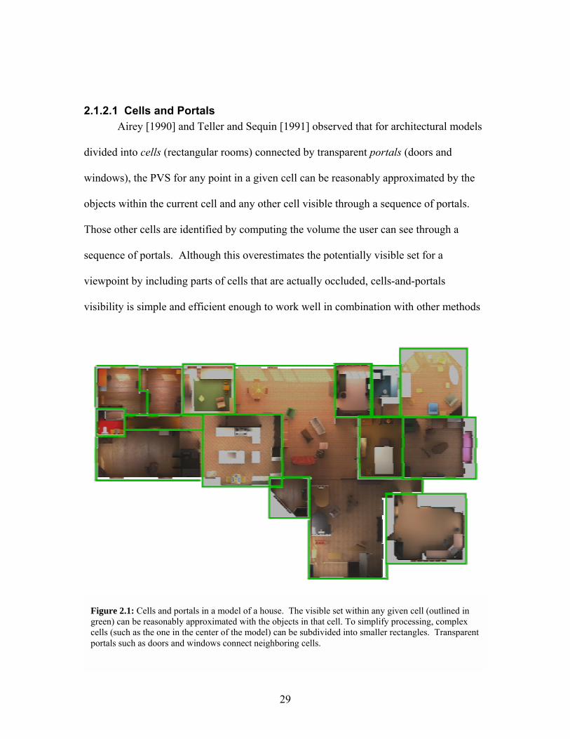
29

2.1.2.1 Cells and Portals Airey [1990] and Teller and Sequin [1991] observed that for architectural models

divided into cells (rectangular rooms) connected by transparent portals (doors and

windows), the PVS for any point in a given cell can be reasonably approximated by the

objects within the current cell and any other cell visible through a sequence of portals.

Those other cells are identified by computing the volume the user can see through a

sequence of portals. Although this overestimates the potentially visible set for a

viewpoint by including parts of cells that are actually occluded, cells-and-portals

visibility is simple and efficient enough to work well in combination with other methods

Figure 2.1: Cells and portals in a model of a house. The visible set within any given cell (outlined in green) can be reasonably approximated with the objects in that cell. To simplify processing, complex cells (such as the one in the center of the model) can be subdivided into smaller rectangles. Transparent portals such as doors and windows connect neighboring cells.

30

such as view-frustum culling. Luebke and Georges [1995] extended cell-based visibility

by treating mirrors as a special case of portals. Moreover, they use a fast, conservative

approximation to identify nearby visible cells instead of Sequin and Teller�s exact sight-

line computations. The intuition behind the approximation is that a cell C is visible if the

user can see into it through a sequence of portals P1, P2,�, PN. The �is visible� relation

is approximated as �the bounding boxes of the portals P1, P2, �, PN leading from the

current cell to the target cell intersect in screen space�. This approximation can be

computed efficiently.

The chief drawback of cells and portals is that it is not useful in environments that

do not exhibit a natural subdivision. Funkhouser et al. [1992, 1996] describe a

walkthrough system for architectural environments that uses geometric levels of detail

plus cells-and-portals visibility culling for rendering acceleration and cell-based

potentially visible sets for memory management. Their system computes the PVS for a

viewpoint from the PVS for the cell containing the viewpoint as well as for any cell

visible through a sequence of portals from that viewpoint. Objects for cells near the

visible regions are prefetched for future use as available time and memory permit.

2.1.2.2 Volume visibility using object-based occlusion Cells-and-portals visibility exploits the property that in architectural environments,

the walls of a room effectively occlude most of the rest of the model from any point

within that room. Occlusion-culling algorithms for less constrained environments can

function similarly by constructing a set of occluders for a given view region.

Schaufler et al. [2000] pre-compute visible sets in 2.5-dimensional environments

such as cities and terrains using the insides of opaque objects (buildings) as occluders.

31

They project buildings down onto the ground plane, then construct a quad-tree so that

every voxel in the tree is either completely inside a building (opaque) or completely

outside a building (transparent). The transparent voxels form the view regions for the

environment. For each view region, a set of blockers is assembled from nearby opaque

voxels. The volume occluded by each blocker is constructed and used to eliminate

portions of the scene that are definitely invisible. Moreover, opaque objects that are

partially within the occluded volume are added to the blocker list, further increasing the

amount of the scene that can be culled.

Durand et al. [2000] present a scheme for visibility preprocessing using extended

projections of convex occluders. For each viewing region, planes are swept through the

environment at a set of discretized depths. Objects are selected to serve as occluders

using a method similar to the one presented in [Zhang et al., 1997]. The algorithm

conservatively estimates the potentially visible set by contracting the volume blocked by

each occluder (similar to finding the umbra of an object) and expanding the bounding

boxes of potentially visible objects to account for the range of viewpoints possible within

the view region. As planes are swept through the environment, the occluder projections

are used to test for objects whose extended bounding boxes are completely blocked. This

method avoids the discretized scene representation required by [Schaufler et al., 2000]

but is restricted to convex occluders. Concave objects are used as blockers by computing

a series of 2D slices where they intersect the sweep plane and treating each of those slices

as a set of independent, convex occluders. Although this approach will not falsely

classify objects as invisible, the discretized sweep of concave occluders can fail in

situations where large parts of an object lie between the different slices. The authors

32

propose handling such situations by treating each individual polygon as an independent

occluder.

The occlusion culling methods described so far are conservative and approximate.

Although they may incorrectly classify objects as visible, they offer some guarantee that

no object will ever falsely be classified as invisible. Nirenstein et al. [2002] present an

exact algorithm that computes the potentially visible set of objects from a particular

region. Their method finds the set of line segments from the view region that can

possibly see an object. These sets are represented in Plücker space, a 5-dimensional

abstraction in which all valid lines are represented as points on a certain hypersurface.

Within this space, constructive solid geometry operations are used to account for the

changes in visibility from a region to an object caused by an occluder. An object is

deemed visible with respect to a view region if any line segments from the region to the

object remain after all of the blockers have been accounted for.

2.1.3 Geometric simplification Geometric simplification methods are another well-studied form of rendering

acceleration. Where visibility culling methods reduce the rendering burden by

eliminating objects known to be invisible, geometric simplification techniques lower the

effort needed to render each object by removing detail that will not be visible in the final

image. For our purposes, simplification schemes can be classified as either static or

dynamic depending on whether they create a discrete set of representations offline or

maintain a single version of an object that is updated often at runtime. More thorough

surveys can be found in [Erikson 2000] and [Garland and Heckbert 1997].

33

2.1.3.1 Static Simplification Static simplification methods start with an original set of primitives and create a

discrete set of approximations, each at a different level of detail (LOD) with respect to

the original. An error measure is typically stored along with the simplified sets of

primitives. At runtime, an LOD is chosen for each object based on the view parameters

and the error measure. Systems can use this information either to maintain a constant

image quality by selecting the coarsest LODs with an error beneath the maximum

tolerable level or to maintain a minimum frame rate by selecting the most detailed set of

LODs possible without exceeding a certain rendering budget.

One approach to static simplification taken by Eck et al. [1995] involves

decomposing a polygonal mesh into a set of wavelet coefficients. A coarse

representation of the input primitives is created using only a few coefficients. Finer

levels of detail are obtained by using more coefficients in the reconstruction. This signal-

processing approach is similar in concept to lossy image compression methods such as

JPEG and JPEG2000.

Many simplification methods operate by progressive decimation of an input mesh.

They typically proceed by maintaining a current mesh along with some error

representation, then performing simplification operations one at a time until some error

bound is met. Cohen et al. [1996] compute two envelopes around the original polygonal

mesh, one outside and one inside, that are free from self-intersections. The mesh inside

the envelopes is simplified by progressively removing vertices and re-triangulating faces

until any further vertex removal would cause the mesh to intersect either of the envelopes.

The error in the simplification can be bounded by constructing the envelopes to lie within

a user-specified distance of the original mesh.

34

Surface simplification can also be accomplished through sequences of edge

collapses instead of vertex removals. Edge collapses simplify the topological operations

that must be performed on the mesh: whereas removal of a vertex can require that many

faces be re-triangulated, an edge collapse will typically remove one or two triangles and

replace one or two vertices without changing the topology of their incident faces. Hoppe

[1996] creates progressive meshes by computing a sequence of edge collapse operations.

The output of the simplification is a sequence of operations that refine an initial drastic

simplification one edge at a time until finally resulting in the original object. A mesh can

be created at any desired level of detail by performing only some prefix of the list of

refinement operations.

Cohen et al. [1997, 1998] describe algorithms that track error in surface attributes

(e.g. the maximum screen-space deviation of any pixel in a surface texture from its

original location) as well as in geometry. Garland and Heckbert [1997] present an

elegant approach based on error quadrics that allow efficient computation of the squared

distance from a point to a plane. Error quadrics are 4x4 matrices that allow fast

computation of the distance between a point and one or more planes. Their major

advantage as an error measure for simplification is that they can be combined in the

following linear fashion: an error quadric that computes the sum of the distances from

two planes A and B to a point P is simply the sum of the quadric that computes the

distance from A to P and the quadric that computes the distance from B to P.

Garland and Heckbert�s approach to polygonal simplification with error quadrics

is an incremental, greedy approach. To begin, they create an error quadric for every

polygon in the mesh that represents the plane containing that polygon. If the user wishes

35

to maintain sharp edges and boundaries as well as surface position, error quadrics may

also be introduced that represent those features. Next, they compute an estimate of the

simplification error introduced by collapsing each edge in the mesh. Since an edge

collapse merges two vertices (the endpoints of the edge) into a single new vertex, the

simplification error is represented as the distance between the new vertex and the planes

in the original polygonal mesh. The error quadrics assigned to the endpoints of an edge

are added and then inverted to help find the optimal position for a merged vertex. Once

the merged vertices and error estimates have been computed for each edge in the mesh,

simplification proceeds by identifying the edge with the least simplification error,

collapsing it, and updating the connectivity of nearby polygons. Error quadrics and

merged vertices are also updated for edges whose endpoints were affected by the edge

collapse.

Since geometric simplification with quadric error metrics does not depend on

mesh topology, it can handle arbitrary input geometry, including unstructured �polygon

soup�. An extension described in [Garland and Heckbert 1998] generalizes the error

quadric to incorporate color and texture information as well as surface position.

One of the drawbacks of simplification using quadric error metrics is that it does

not account for surface area when merging vertices. This can cause parts of an object to

disappear or be greatly distorted when creating drastic simplifications. Erikson [GAPS

paper] modifies Garland and Heckbert�s method by choosing simplification operations

that preserve the mesh surface area and by introducing an adaptive distance threshold

when constructing vertex pairs for potential merges. Errors in surface attributes such as

color, texture coordinates, and normals are managed along with surface deviation as a

36

simplified mesh is being constructed. In addition, Erikson demonstrates how drastic

simplifications of a large environment can be created by simplifying objects as a group

(thus allowing topological merges between objects). Such grouped simplifications are

called hierarchical LODs (HLODs).

2.1.3.2 View-dependent LODs Level-of-detail schemes that compute incrementally simpler representations of an

object can be viewed as constructing a tree structure called a vertex merge tree. The

nodes of this tree are the vertices of the representation of the object(s) being simplified,

with the original vertices in the leaf nodes. The edges in the tree correspond to the

individual simplification operations. The topology of the mesh is stored separately, with

instructions for updating it stored in each edge. The root of the tree is formed by taking

the process of simplification to its extreme, reducing the entire set of original primitives

to a single vertex.

Static simplification schemes, as described in the previous section, take periodic

snapshots of the current set of primitives as the vertex merge tree is created. Although

static methods create high-fidelity approximations with little per-frame overhead in

rendering, their strength is also their disadvantage: a set of discrete levels of detail must

be chosen during simplification and cannot be modified at runtime. This can result in

poor performance when none of the different LODs are a good match for the viewing

parameters. Consider the example object shown in Figure 2.2. If the user looks at the

cylinders from close by, the rendering system must choose between displaying the entire

object at high fidelity, thus rendering even distant or invisible regions at the same high

fidelity and reducing frame rate, and displaying the entire object at low fidelity, which

37

maintains a high frame rate but will tend to expose simplification errors close to the

user�s viewpoint. View-dependent simplification schemes can handle such configurations

by computing a representation of an object where the particular simplification depends on

what the user can see. View-dependent simplification offers the ability to use different,

continuously varying levels of detail across different parts of a single object, at the cost of

runtime processing overhead to maintain the current simplification.

Luebke and Erikson [1997] propose a hierarchical, view-dependent simplification

scheme based on vertex clustering. They create a vertex merge tree by repeatedly

grouping two or more vertices into a single point representing both vertices. The

particular choice of vertices to be clustered can be determined by nearly any

simplification method. At runtime, a list of active nodes in the vertex tree keeps track of

the current simplification. Active nodes represent vertices that will be rendered and are

annotated with information about the faces in which those vertices participate. The

simplification is refined or coarsened by folding an active node into its parent (thus

removing vertices from the current environment) or by unfolding an active node into its

children (thus adding vertices into the environment). Nodes are folded and unfolded

according to criteria such as potential screen-space simplification error, preservation of

silhouette edges and object boundaries, and a per-frame rendering budget.

38

Similar approaches were developed by Varshney and Xia [1996] and Hoppe

[1997]. The authors reorganized the sequence of edge collapses used in progressive

meshes into a merge tree, thus allowing a given refinement operation to be performed

without requiring that all of its predecessors in the sequence be performed as well. Both

methods require manifold meshes as their input and track mesh properties in order to

prevent the creation of a simplification that folds back on itself, thus creating a non-

manifold surface. View-dependent refinement is carried out in a manner similar to that

of Luebke and Erikson, with a set of active nodes being folded (collapsed) or unfolded

(split) according to criteria such as visibility, screen-space error, boundary preservation,

Figure 2.2: A difficult case for static simplification methods. This group of gas cylinders is represented as a single object in the Double Eagle environment. In views such as the closeup in the lower image, a high level of detail will render invisible cylinders using many polygons (leading to a low frame rate), whereas a low level of detail will maintain a high frame rate at the cost of poor fidelity in the small portion of the model that is actually visible. View-dependent simplification schemes can handle such cases by rendering different parts of a single object at different levels of fidelity.

39

or surface attribute preservation. Unlike Luebke and Erikson�s approach, the requirement

that the input surfaces form a valid mesh prevents simplification operations from

collapsing vertices that belong to different objects. As a result, topological

simplifications that merge separate objects in an environment are not possible. Such

merges are forbidden when creating drastic simplifications because they could cause

objects to shrink or disappear entirely.

2.1.4 Image-Based Rendering The rendering acceleration methods described so far operate on geometric

representations of objects. In complex environments composed of thousands of objects

and tens of millions of primitives, it is quite common for visibility methods and level-of-

detail techniques to yield a potentially visible set of objects containing more primitives

than there are pixels in the frame buffer. For example, the view of the interior of the

Figure 2.3: This view of the interior of the power plant environment contains over 8 million polygons inside the view frustum. The image itself was rendered at 1024x1024 resolution. As a result, at most one in eight polygons rendered are visible in the final image. Image-based rendering methods accept the high but constant cost of processing every pixel in an image in order to avoid such drastic overdraw.

40

power plant model shown in Figure 2.3 contains over 8 million polygons in the view

frustum but only about 1 million (1024x1024) pixels in the frame buffer. Image-based

rendering methods operate by replacing geometry with a set of sampled representations

(commonly pixelated images augmented with per-pixel depth). This allows a system to

render the sampled primitives with per-pixel complexity proportional to the number of

samples taken and the resolution at which each sample is acquired.

Most image-based rendering (IBR) methods are based around the notion of the

plenoptic function [Adelson and Bergen 1991] that describes light transport in an

environment. The plenoptic function is defined as follows:

( )tVVVPp zyx ,,,,,, λφθ=

This maps a 3-dimensional point (Vx, Vy, Vz), a viewing direction (θ, φ), a

wavelength λ, and a time t to an intensity value p. The plenoptic function can be

viewed as giving the incident radiance in all directions and all wavelengths around

each point in an environment. We assume here that free space does not affect

intensity values, although the plenoptic function itself does not preclude the use of

participating media such as fog or smoke. Moreover, most image-based rendering

methods assume a static environment and do not include time as a parameter. The

goal of IBR is to construct an approximation of the plenoptic function at some

viewpoint V´ given samples of its values around nearby points V0, V1, V2, �, VN.

The expectation is that the high but constant complexity of rendering from images

will be less expensive than rendering geometry that may place several different

41

polygons in each pixel of the screen. In this section we survey a few common

image-based rendering techniques.

2.1.4.1 Texture maps Texture mapping [Catmull 1974, Blinn and Newell 1976] is the simplest image-

based rendering technique. By rendering an image on the surface of (often simple)

geometry, dense surface detail can be added to a scene without the associated cost of

dense geometry. Systems such as Lippman�s Movie Maps [1980] replace the entire

environment with a panoramic image mapped onto a sphere surrounding the viewpoint.

By using panoramic textures, the Movie-Maps system was able to accommodate panning,

tilting, and zooming the user�s view of a particular texture map. Translation through the

environment was accomplished by jumping to another location from which one of the

panoramic textures had been acquired. Interpolation between these viewpoints was not

supported.

The chief limitation of texture maps as a modeling primitive is that they do not

contain the information necessary to reconstruct parallax effects in the sampled

primitives as the user�s viewpoint changes. Rendering artifacts due to the lack of

parallax can be alleviated by substituting new texture maps acquired from locations

closer to the current viewpoint. However, acquiring and storing enough texture maps to

alleviate parallax artifacts can quickly become prohibitively expensive.

2.1.4.2 Single-source image warping Parallax in visible surfaces is a function of the distance from the viewpoint to

points on the surface. By adding depth information to each pixel in a texture map, it

becomes possible to reconstruct parallax effects for the portions of surfaces visible in that

42

texture map. McMillan and Bishop [1995] acquire a set of cylindrical images that

enclose a number of viewpoints in an environment, then extract per-pixel disparity (the

inverse of depth) by computing the image flow field between pairs of panoramas. User-

specified correspondences between panoramas are used to estimate the relative

transformations between viewpoints. Novel views of the sampled environment can be

reconstructed by constructing an image flow field from the disparity values that warps

one panorama into a view appropriate to the new location. During reconstruction, a

cylindrical panorama is divided into toroidal sheets that are traversed in a pattern that

maintains a back-to-front ordering of the individual samples. Since it does not depend on

having per-pixel disparity available as part of the rendering process, but rather extracts

this information from the panoramas themselves, McMillan and Bishop�s approach is

applicable to real-world environments as well as synthetic data.

Oliveira and Bishop [2000] describe an extension to standard texture mapping

that provides results similar to image warping. Standard texture maps are augmented

with orthogonal displacements (depth) at each pixel to produce relief texture maps.

These displacements are used to warp each texture for each frame in order to account for

depth parallax and occlusion. The pre-warped textures are then rendered using standard

texture mapping hardware. By taking advantage of the graphics pipeline, relief texture

maps can be integrated with ordinary geometry. However, since relief textures are

ultimately given to the graphics hardware as flat images without depth, correct

interpenetration between geometry represented in relief textures and geometry

represented as polygons is often misrepresented.

43

Image warping techniques that use a single source image, whether panoramic or

not, only contain information about the first surface visible at each pixel. As a result,

new viewpoints that should be able to see surfaces that are occluded in the source image

will show artifacts in the reconstructed image. The nature of these artifacts depends on

the particular reconstruction method. If samples from the source image are treated as

disconnected points, cracks can appear in the reconstruction. If a group of samples are

treated as a connected surface and gaps are filled using interpolation, stretching and

smearing artifacts called skins can become visible. Figure 1.7 shows examples of both

cracks and skins as compared with a geometry-only rendering. These artifacts can often

be alleviated by warping multiple source images into the same camera space, as described

in the next sections.

2.1.4.3 Multiple-source image warping Surfaces in an environment that are occluded from one viewpoint are usually

visible from a different location. This suggests that image warping using multiple source

images taken from distinct viewpoints may be able to provide a more complete

reconstruction than any single image used alone. William Mark [1999] describes a

rendering acceleration system that uses image warping to interpolate between pairs of

rendered images. The system is intended to operate under conditions where high-quality

images are available at low update rates, as when the images are being transmitted over a

network. Pairs of images are selected that are likely to contain most of the surfaces

visible from a novel viewpoint, then warped into a common camera space for display to

the user. Regions where the surface being reconstructed is visible in both source images

are handled by compositing different warped samples.

44

2.1.4.4 Layered depth images Image warping using multiple source images is capable of providing high-quality

reconstructions while reducing occlusion artifacts. However, warping the entirety of two

source images can be overkill in situations where a single source image contains most of

the surfaces visible in the reconstruction. Layered depth images (LDIs) [Shade et al.,

1998] address this problem by providing a data structure that can store multiple source

images with little duplication of already-sampled surfaces. An LDI consists of a

rectangular array of pixels plus depth, just as in standard image warping; however, each

location in the array is allowed to contain multiple samples. The samples for a single

pixel location in a layered depth image can be obtained by tracing a ray through the

center of the pixel and creating a sample for the first N surfaces intersected along the

ray�s path. Alternately, the lists of samples can be created by warping a series of source

images into the LDI�s camera space. Whenever an element of the source image falls

within a particular pixel, it is compared with the samples already stored there and

discarded unless it represents a new surface. This latter method of construction results in

an LDI that contains most of the visible surfaces from each source image without

duplicating surfaces visible from more than one source viewpoint. Views of the

environment from novel locations are reconstructed from an LDI using a warping

algorithm similar to those described above in [Mark 1999] and [McMillan and Bishop

1995]. Chang, Bishop, and Lastra [1999] propose the LDI tree, composed of an octree

with a single layered depth image associated with each node. The resulting structure

preserves different sampling densities in different parts of the environment, thus

overcoming the limits imposed by the single fixed resolution of Shade�s original layered

depth images.

45

2.1.4.5 Light Fields and Lumigraphs The methods described so far represent the plenoptic function using point samples

of visible surfaces. Light fields [Levoy and Hanrahan 1996] and lumigraphs [Gortler et

al. 1996] take a different approach. Both methods represent a portion of an environment

as a 4-dimensional set of rays that originate on one quadrilateral and pass through another.

Novel views of the environment are reconstructed by finding the rays that most closely

approximate the view ray for each pixel of the new view.

Levoy and Hanrahan [1996] construct a 4-dimensional light field from a set of

sampled or digitized images. Each image is broken up into a set of rays from the camera

through an image-space location. These rays are parameterized in 4 dimensions

according to their intersections with two quadrilaterals, one near the rays� origins and one

nearer to the objects. In order to reduce aliasing in reconstructed views, the rays in a

light field are filtered using a 4D low-pass filter. Although this pre-filtering process

discards some of the information present in the database of rays, the effect is much the

same as blurring due to depth of field. The storage requirements of light fields are

reduced using a combination of vector quantization and entropy coding.

Gortler et al. [1996] build lumigraphs using a 2-plane parameterization similar to

the one used for light fields. Rather than pre-filter the database of rays, a lumigraph

resamples the database onto 4-dimensional basis functions. Gaps in the data are filled in

by downsampling the data to a lower resolution, then using the average values from that

lower resolution to approximate the values in unsampled locations. When available,

information about the geometry of the scene can be used to build a better reconstruction.

Given a novel viewpoint, rays are traced through each pixel to find an appropriate set of

4D coordinates for each sample. The intersections of these rays with a coarse geometric

46

representation of the scene are used to change the 4D sample coordinates to find rays that

better approximate the view. If no such information is available, reconstruction proceeds

with the assumption that all objects lie at a constant depth. Isaksen, McMillan, and

Gortler [2000] change this assumption by maintaining a camera surface containing all of

the viewpoints of the input images instead of resampling the rays during construction.

This allows dynamic reparameterization of a light field at render time in order to simulate

effects such as different focal lengths and associated blurring due to depth of field.

Chai et al. [2000] address the construction and rendering of light fields from a

signal-processing perspective. They describe the frequency spectrum of a 4D light field

as a function of the depths of the surfaces visible in the environment and derive bounds

on the shape of the Fourier transform of 2D slices of the light field. These bounds are

used to establish optimal sampling densities for use during acquisition. Moreover, this

sampling approach can make use of information about the underlying scene geometry by

dividing the scene into depth layers and adapting the shape of the reconstruction kernel to

each layer in turn.

Because light fields and lumigraphs represent a space of rays rather than a set of

surface samples, they are able to capture view-dependent phenomena such as specular

highlights and reflections. However, accurate sampling of such phenomena is often

costly due to the many samples and high resolution needed to capture their significant

high-frequency content.

2.1.5 Hybrid rendering acceleration methods incorporating IBR and geometry Each of the image-based rendering methods described in the previous section has

been used alone to render entire environments. It is also possible to use IBR as a

47

rendering acceleration technique in combination with geometric methods such as

visibility or occlusion culling and level-of-detail simplification. In this section we survey

rendering acceleration techniques that incorporate concepts from both image-based

rendering and standard geometric methods. These techniques are all oriented toward the

creation of image-based impostors, which are simplified representations of parts of the

environment that can stand in place of the objects they represent. By comparison, the

level-of-detail methods described earlier can be interpreted as creating geometry-based

impostors.

2.1.5.1 Replacing groups of objects with textured clusters Maciel and Shirley [1995] create image-based impostors for an environment by

partitioning the objects in a scene using an octree. Individual objects are treated as the

leaf nodes in a tree. The edges of the tree are determined by the octree structure: if an

octree cell A encloses smaller cells B, C, and D, then node A in the tree is the parent of

nodes B, C, and D. Leaf nodes containing single objects are assigned as children of the

smallest octree node that completely encloses the object. Once this hierarchy has been

established, a set of impostors is created for each node in the tree. The impostors in this

case are a set of six texture maps that are drawn on the sides of an octree cell. Objects

within a cell are rendered into a texture map using orthographic projection. At runtime,

the system chooses a set of nodes in the tree that collectively represent all objects in the

environment at the best possible quality while remaining within a certain rendering

budget. Rendering quality is computed using a view-dependent cost/benefit function for

each node in the tree.

48

2.1.5.2 Replacing distant objects with flat textures or LDIs Aliaga and Lastra [1997] accelerate cells-and-portals visibility culling by

covering portals with textured impostors. This reduces the potentially visible set to the

contents of the current cell plus the impostors for visible portals instead of the geometry

visible in all cells the user can see. To provide for the reconstruction of depth parallax,

several textures are computed for each portal from several different viewing directions.

At runtime, the texture whose view direction best approximates the user�s view is chosen

as an impostor. In order to prevent distracting �popping� artifacts when the system

switches from impostors to rendering actual geometry, objects in nearby cells are warped

to match their positions in the portal texture. This warp is smoothly relaxed to return

objects to their proper positions as the user moves into the new cell.

Later work [Aliaga and Lastra 1999] generalizes this approach in order to replace

arbitrary parts of an environment with image-based impostors. The environment is

partitioned into objects that are grouped using an octree. A regular grid of viewpoints is

then established throughout the model. For each of these viewpoints, a number of view

directions are examined to find situations where the size of the visible set of primitives

exceeds the rendering budget. In such cases, a set of octree nodes are identified for

replacement using impostors. At runtime, objects in nearby octree cells are rendered as

geometry and layered depth images are used as impostors for faraway objects. System

resources turned out to be a bottleneck for this method: the per-pixel processing to warp

LDIs required significant CPU power, and the expense of paging impostor data in from

disk limited the user�s maximum walking speed.

49

2.1.5.3 Billboard clouds Decoret et al. [2002] propose an impostor representation that replaces an object

with a group of flat, textured, partially transparent polygons (called billboards). Their

approach is to compute a set of planes that collectively capture the surfaces in a model.

A plane captures a given face if the distance from that face to the plane falls within some

user-specified error threshold. Rather than solve the (presumed difficult) global

optimization problem of finding the best fit for some minimum number of planes, the

authors cast the problem as a greedy, incremental optimization. The polygons in an

object are considered as points in a 3-dimensional plane space. Each point in this space

is surrounded by a scalar field whose value at any point corresponds to the simplification

error incurred by replacing the corresponding face with one particular plane. The scalar

fields for all faces in an object are combined to give an overall density function.

Optimization proceeds by discretizing this density function and repeatedly

selecting the location with the highest density. This location corresponds to a plane that

captures some set of faces in the original model. That plane is added to the impostor as a

new billboard, the corresponding faces are removed from the model, and the density

induced by those faces is removed from the scalar field. The construction process

terminates when the density function falls below a user-specified threshold at all points.

Billboard clouds can be created with either view-dependent or view-independent

simplification criteria by modifying the values of the scalar field generated by each face.

Their advantage as an impostor representation lies in their low geometric cost: typical

billboard clouds contain under 100 textured polygons. However, the cost of texture maps

for each of these polygons can grow expensive. This expense could be reduced by

storing only the meaningful (non-transparent) pixels in each texture map instead of the

50

entire image. The authors have demonstrated billboard clouds as an impostor

representation only in outside-looking-in environments: their properties in inside-

looking-out environments have yet to be discussed.

2.1.5.4 Textured depth meshes The image-based rendering methods we have described so far have each had one

of two limitations. Texture maps are supported and accelerated by nearly all current

graphics hardware but on their own cannot reconstruct depth parallax. More complex

approaches such as image warping and layered depth images do indeed show depth

effects but are not supported by current graphics hardware, thus placing most of the

rendering load on the CPU. In this section we describe textured depth meshes (TDMs),

an image-based impostor format compatible with the standard graphics pipeline

Darsa, Costa, and Varshney [1997] describe an image-based rendering system that

begins with a cube environment map containing both color and depth information for a

set of viewpoints in a model. A triangle mesh is created for each face of each

environment map using the information in the depth buffer. The density of the mesh is

related to discontinuities in the source image as well as the depth of the samples being

represented: nearby samples will be more densely triangulated than distant ones, and

many triangles will be used to preserve sharp image-space discontinuities. Color

information is applied to these depth meshes using projective texturing rather than

standard texture mapping in order to preserve correct perspective effects. The authors

present a variety of interpolation and blending methods to reconstruct views from

multiple environment maps, including simple superposition (relying on the graphics

hardware to resolve depth and occlusion) and view-dependent weighted blending based

51

on the distance between the viewpoint and the sample locations for nearby cube maps.

Since these textured depth meshes are created from single source images, they suffer

many of the same visibility artifacts as in single-source image warping, including skins

and cracks.

Decoret, Darsa, and Sillion [1999] present a thorough discussion of the artifacts

introduced by textured depth meshes. They classify these artifacts as resolution

mismatch, where the user approaches a TDM closely enough to see the texture sampling;

deformation by the impostor representation, where objects in a TDM appear distorted

due to insufficient sampling of their underlying geometry; incomplete representation,

where objects are omitted entirely from a reconstruction as a result of not being sampled

at all; rubber sheets (which we call skins), which are the artifacts described earlier that

result from linear interpolation across depth discontinuities; and finally cracks, which are

holes in the textured depth mesh that might otherwise be covered by skins. They propose

a multi-meshed impostor representation for distant geometry that reduces the prevalence

of such artifacts by allocating different objects to different meshes entirely. By

restricting viewing regions to 1D line segments and the shape of the environment to 2.5D

buildings (in particular, an urban scene), it becomes possible to group objects into layers

based on whether or not they can cause visibility events (occlusions or exposures) of a

certain user-specified magnitude. At runtime, multi-meshed impostors are used to

approximate distant geometry while nearby objects are rendered in the usual fashion.

When extra time remains in the rendering pipeline, nearby impostors are updated

dynamically by rendering their underlying objects from the user�s current viewpoint.

Since the artifacts in impostors grow worse as the user translates away from the sample

52

viewpoint, this update results in greater image fidelity while the user remains close to the

new viewpoint.

Aliaga et al. [1999] describe a system for rendering large architectural models that

uses textured depth meshes as impostors. They generalize portal textures [Aliaga and

Lastra 1997] to accommodate environments that do not exhibit an intrinsic subdivision

into cells. The environment is first divided into rectangular virtual cells. For each cell, a

concentric, cubical cull box is created to divide the model into near and far geometry.

The size of the cull box is chosen to be as large as possible while containing less than a

set number of primitives. (Figure 2.4) During preprocessing, a set of impostors is

created for each face of each cull box. The authors describe experiments with flat

texture-mapped quadrilaterals, image warping, and textured depth meshes as impostors.

Impostor view frustum

Virtual cells

Cull box

Figure 2.4: Virtual cells for replacement of distant geometry. All objects inside the cull box form the near field and are rendered as geometry. All objects outside the cull box form the far field and are replaced with image-based impostors. Each cell is associated with a single cull box. Adjacent cells do not overlap, although their cull boxes often do.

53

Textured depth meshes were ultimately chosen to replace geometry outside the cull box

due to their combination of compatibility with the graphics pipeline and the presence of

parallax effects. At runtime, objects that intersect the cull box are rendered with a

combination of static level-of-detail simplification and occlusion culling. The TDMs

created during preprocessing stand in for all geometry outside the cull box. In addition to

the rubber-sheet �skins� reported by Decoret, Darsa, and Sillion, the authors report that

changing from one cell to another in the model (and hence from one set of impostors to

another) causes a distracting �pop� in the appearance of distant geometry.

Jeschke and Wimmer (EG2002) describe two different approaches to the creation

and display of textured depth meshes. In �Layered environment-map impostors for

arbitrary scenes�, they divide the scene into near and far geometry using a cull box as in

[Aliaga et al. 1999]. However, instead of using a single textured depth mesh for each

face of the cull box, they divide distant geometry into many layers and create an

environment map for each layer. The distance between successive layers is chosen so

that adjacent layers cannot move more than one texel against one another for any

viewpoint in a cell, thus guaranteeing that cracks will not appear in surfaces that cross

between layers. The size of the cell is dictated by the number of layers in the impostor

and the maximum permissible translation between one layer and the next. The authors

report that a view cell size of 10m by 10m, an environment map resolution of 512x512,

64 layers of environment maps, and a maximum displacement of 1 texel dictates that the

edges of the cull box be 42 meters away from the center of the view cell. Occluded

texels in the layers of environment maps are detected and removed in order to reduce the

storage requirements. Since each layer of each environment map can require that the

54

entire model be drawn and the frame buffer captured, this approach can be prohibitively

expensive when attempting to guarantee high fidelity for environments where the near

field distance is under ten meters.

In �Textured depth meshes for real-time rendering of arbitrary scenes�, Jeschke

and Wimmer [2002] use the same multi-layered capture process described above.

However, instead of a set of environment maps, the far-field images are used to create a

voxelized representation of distant geometry. Regular, dense polygonal meshes are

created over these voxels and then simplified by repeatedly collapsing the shortest edges

in each mesh. Edge collapses are permitted or forbidden according to whether or not the

resulting mesh would cover all of the underlying voxels as well as the effect the collapse

could have on mesh boundaries. At runtime, textures are applied to the meshes using the

same projective texturing technique employed in [Darsa et al. 1997, Decoret et al. 1999,

Aliaga et al. 1999]. As with the layered environment map representation described above,

the acquisition of many layers of the environment for each face of each cell as well as the

increasing number of layers necessary to guarantee high-fidelity reconstruction can be

significant bottlenecks in complex environments.

2.2 Image and video compression

One common feature of the image-based rendering methods described in the

previous section is high storage cost. In this section we survey approaches to

compressing still images and video sequences as a means of alleviating that storage cost.

2.2.1 Still image compression In general, the amount of information contained in a still image is far lower than

the amount of storage space needed to represent it in an uncompressed form. Still image

55

compression techniques reduce this storage cost by transforming the uncompressed data

into a more compact form. There are two major approaches to image compression. First,

lossless compression techniques encode all the information in the original image,

allowing the input to be reconstructed exactly. Second, lossy compression techniques

discard parts of the input that are judged to be unimportant. Common criteria for this

judgment include the sensitivity of the human visual system to different spatial

frequencies. Although the input to a lossy compression scheme cannot be exactly

reconstructed, the intent is to produce a result that is indistinguishable from the input with

respect to a human observer. In this section we describe a representative example of each

type of compression. We do not intend a complete survey of image compression: the

examples in this section are intended primarily to provide context for the video

representations to follow.

2.2.1.1 Lossless image compression (PNG) The Portable Network Graphics (PNG) [Roelofs 1999, Boutell 1997] standard

was designed to replace the older GIF image format [GIF89a] as a means of lossless

compression of still images. The file format consists of a series of chunks describing the

chromaticity, gamma, and dimensions of the image as well as the actual compressed

intensity values. PNG achieves its compression through an entropy coding scheme

similar to the method described in [Lempel and Ziv 1977] that represents a sequence of

integers using Huffman codes. Data may be transformed using one of five filters to make

it more amenable to entropy coding. These filters are as follows:

1. No transformation. Image data is left unchanged.

56

2. Horizontal subtraction. The filter produces the difference between each

byte and the corresponding byte of the previous pixel in a scan line.

3. Vertical subtraction. The filter produces the difference between each byte

and the corresponding byte of the pixel in the scan line immediately above the

current one.

4. Average. The filter uses the average value of the appropriate bytes in the

pixels to the left and above the current position to predict the value of each

byte in the current pixel.

5. Paeth predictor. The filter computes a linear function of the pixels to the left,

above, and upper left of the current position. The neighboring pixel whose

value is closest to the computed value is used as a predictor.

PNG encoders commonly select a different filter for each scan line according to

which method produces the smallest sum of absolute values of outputs. The choice of

filter can greatly enhance the performance of entropy coding.

PNG�s main strengths as an image compression format include a progressive

representation of image data. This allows image decoding and display to begin when

only a small fraction of the data have been received by the decoder. As more information

becomes available, the quality of the decoded image can be improved, until finally the

original image is reconstructed at the end of transmission. In addition to its utility when

images are being sent over a network (especially in Web pages), progressive transmission

and decoding can also be used in an image-based rendering context. If an image is far

enough away from the user that its full resolution is unnecessary, a progressive

57

representation can allow a rendering system to avoid wasting effort decoding information

that will be invisible to the user. Moreover, since the entropy-coding stage of PNG

compression treats an image as a linear sequence of bytes, it is well suited to images

containing large areas of uniform color. Images of synthetic environments often exhibit

this property. Finally, PNG�s lossless nature can be either a strength or a weakness

depending on the circumstances in which it is applied. If images are intended for use in

mathematical operations such as bump mapping or as lookup tables for shading

computations, lossless compression is of critical importance: although a lossy method

may produce an image indistinguishable from the original to the naked eye, using that

same image as input to equations may give results that are completely wrong. However,

images of complex or natural scenes that are intended for display are often a poor fit for

PNG�s capabilities. All information in the input will be present in the compressed

representation whether or not it is perceptually significant. Moreover, the random noise

inherent in samples of the real world (e.g. film grain) often causes entropy coding

schemes to perform poorly.

PNG�s efficiency at representing large areas of uniform color and sharp

boundaries suggests that it might be a good match for image-based impostors. However,

its lossless nature can sometimes be a significant drawback. First, high-frequency

information in surface textures will be faithfully reproduced even when the process of

impostor reconstruction cannot display such components. Second, broad areas of high-

frequency variation are a difficult case for PNG in general since its mechanisms for

prediction of nearby image values are oriented toward small deviations from a smoothly

varying mean. Such visually rich situations can arise as a result of dense, complex

58

geometry such as the view shown in Figure 2.5 or simple geometry with complex

textures as shown in Figure 2.6.

2.2.1.2 Lossy image compression (JPEG and JPEG2000) The JPEG image compression standard [Pennebaker and Mitchell 1992] was

created by the ISO/IEC Joint Photographic Experts Group for compression of images of

natural scenes. It operates by transforming image data into frequency space using the

discrete cosine transformation (DCT), quantizing the resulting coefficients according to a

model of the human visual system (causing many of the coefficients to fall to zero), run-

length encoding the result to exploit long sequences of zeros in the coefficients, then

entropy-coding the output of the run-length encoder. The user can choose between a

higher compression ratio and increased fidelity to the original image by scaling the

(a) PNG (152 Kb) (a) JPG (66 Kb)

Figure 2.5: Lossy compression techniques can outperform lossless methods in complex synthetic environments. In spite of being optimized for real-world data, lossy JPEG yields results comparable to lossless PNG for less than half the storage space.

59

coefficients in the quantization matrix. In this section we provide a brief overview of the

major components of JPEG compression. These components will also be used in the

video compression methods described later.

2.2.1.2.1 Macroblock Structure In order to reduce the computational overhead of the frequency transformation,

JPEGs are encoded as groups of macroblocks instead of as a linear sequence of pixels.

Each macroblock is transformed into frequency space independently of the rest of the

image. Although this discards the ability to detect and encode frequencies with

wavelengths longer than 32 pixels, block sizes larger than 8x8 do not offer sufficient

improvement in the compression ratio to justify the additional overhead.

Figure 2.6: A simple polygonal scene whose visual complexity is due to surface texture. This view is taken from the house environment. The surfaces are represented using only a few hundred polygons: almost all apparent detail is supplied by texture maps. Lossy JPEG compression achieves an 87% reduction in file size with little or no visible loss of image quality.

(a) PNG (708 Kb) (b) JPEG (82 Kb)

60

2.2.1.2.2 The Discrete Cosine Transform Luminance and color data are transformed from intensity space to frequency

space using the discrete cosine transform (DCT). The DCT is similar to the discrete

Fourier transform in that it produces the same number of coefficients in the output as

there were values in the input. Moreover, DCT coefficients are always real: there is no

need to handle complex numbers as is required for the Fourier transform.

The 8x8 DCT transforms an input matrix x of intensity values to an output matrix

y of frequency values as follows:

+

+

= ∑∑= = 16

)12(cos16

)12(cos4

)()( 7

0

7

0

ππ ljkixlckcyi j

ijkl

where k,l = 0, 1, �, 7 and

=

=otherwise

kifkc1

02

1)(

On its own, this formulation is simple enough for hardware implementation.

However, the DCT has two more properties that make it particularly attractive.

The first useful property of the DCT is separability. The 2D 8x8 DCT can be

computed by first computing eight 8x1 1D transforms (the rows of a matrix), then

computing eight 1x8 1D transforms (the columns of that matrix). The 1D DCT is defined

for an output z and an input x as follows:

∑=

+

=7

0 16)12(cos

2)(

iik

kixkcz π , k = 0, 1, �, 7.

The simplicity of this equation illustrates the attractiveness of the DCT from an

implementation perspective.

61

The second useful property of the DCT is orthogonality. If the DCT is expressed

in matrix form as Y = T X TT, its inverse is X = TT Y T. We view premultiplication by

matrix T as applying the 1D DCT to each row of X. Correspondingly, postmultiplication

by TT applies the 1D DCT to each column. We may therefore invert the 2D DCT by

reversing the order in which the row-by-row and column-by-column 1D DCTs are

applied. Indeed, the equation for the inverse DCT (IDCT) is thus very similar to the

forward DCT:

+

+

= ∑∑= = 16

)12(cos16

)12(cos4

)()( 7

0

7

0

ππ ljkiylckcxk l

klij

This suggests that special-purpose hardware used to compute the forward DCT

can be used without modification to compute the IDCT as well. The reader is referred to

[Bhaskaran and Konstantinides 1997] for a more complete discussion of its properties.

2.2.1.2.3 Perceptual basis for lossy compression The main advantage of JPEG over lossless compression methods is its ability to

discard information that is not perceptually significant. The properties of the human

visual system are exploited in two different ways at two different stages of the

compression process.

First, the human visual system is far more sensitive to luminance information than

to chrominance. Input images are transformed from tristimulus RGB values into YUV

space (luminance plus two chrominance values), then the U and V channels are usually

downsampled by a factor of two in each direction. Although this halves the maximum

frequency that can be reconstructed in the two chrominance channels, the blurring usually

goes unnoticed in the presence of full-resolution luminance data. This subsampling

reduces the storage requirements for an N-by-N-pixel image as follows:

62

Original image (RGB): N * N (red) + N * N (green) + N * N (blue) = 3 N2

Subsampled image (YUV): N*N (Y) + (0.5 N)*(0.5 N) (U) +

(0.5 N)*(0.5 N) = 1.5 N2

During decompression and reconstruction, four 8x8-pixel macroblocks from the

luminance channel are used to fill one 16x16-pixel region in the final image. Since the

two chrominance channels were subsampled by a factor of two in each direction, a single

8x8 macroblock from each of the U and V channels is sufficient to provide color

information for the entire 16x16-pixel region.

Second, the human visual system is more sensitive to certain frequencies than to

others. [Daly 1993] describes an algorithm for measuring visual fidelity based on

frequency content at multiple spatial scales. As a result, DCT coefficients representing

frequencies to which the eye is relatively insensitive can be stored with less precision

than frequencies that are more noticeable. A quantization matrix (described in the next

section) is applied to the DCT coefficients for each macroblock to accomplish this.

2.2.1.2.4 Quantization of DCT coefficients After the intensity values in an 8x8-pixel macroblock have been transformed to

frequency-space coefficients using the DCT, the 64 coefficients are divided by the

corresponding entries in an 8x8 quantization matrix Q. The values in the standard Q

matrix are small for frequencies well-resolved by the visual system, resulting in little loss

of precision, and higher for frequencies to which a human observer is less sensitive.

Quantization also causes many coefficients to drop to zero, further decreasing the amount

of information that will be stored in a compressed JPEG. The user may tune the

63

compression ratio by multiplying each entry of Q by an integer from 2 to 62. A higher

multiplier yields a higher compression ratio.

2.2.1.2.5 Run-length encoding and entropy compression The final stages of JPEG compression consist of arranging the 2D array of

quantized coefficients into a 1D sequence and compressing the result. The 64

coefficients are laid out in zig-zag order (Figure 2.7) in order to group zero-valued

coefficients together. The resulting 1D sequence is run-length encoded to reduce strings

of zeros to a sentinel value plus a count. The output of the run-length encoder is

subjected to entropy coding using a modified Huffman encoding scheme to yield the final

compressed data.

Figure 2.7: Zig-zag order for layout of a 2D array of DCT coefficients into a 1D sequence. This ordering groups zero coefficients together to improve the performance of run-length encoding. The upper left corner contains the DC (constant) term. Horizontal frequency increases from left to right and vertical frequency from top to bottom.

64

2.2.1.2.6 Advantages and Disadvantages of JPEG The JPEG standard was designed for compression of images of natural scenes.

These images are assumed to be destined for display to a human observer after

decompression. By eliminating information at frequencies imperceptible to the human

visual system, JPEG is able to achieve significant compression (sometimes up to 100:1

for very large images, e.g. more than 1 million pixels) with little or no perceptible loss in

visual quality. Moreover, by allowing the user to choose a higher or lower scaling factor

for the quantization matrix, a JPEG encoder can trade off compression against image

quality.

Although JPEG was designed for use on images of natural scenes, it is often

useful when compressing synthetic imagery. In particular, complex environments with

realistic lighting and texture (e.g. the house model shown in Figure 2.1) are good

candidates for JPEG. By contrast, environments with large, smooth color gradients and

sharp boundaries are more likely to show compression artifacts as the quantization factor

increases. Examples from both the house and the power plant environments are shown in

Figure 2.8. The severity of these artifacts can be reduced either by decreasing the

quantization factor (thus reducing the overall compression) or by choosing a quantization

matrix better suited to the properties of the synthetic images under consideration. A

method for creating such quantization matrices is described in [Watson 1994].

65

2.2.1.2.7 JPEG2000 The recent JPEG2000 standard [Taubman and Marcellin 2001] is similar to JPEG

in that it performs lossy compression of still images by quantizing the output of an

Figure 2.8: Synthetic images poorly compressed by JPEG and the DCT. The images on the left are lossless PNGs. The images on the right are JPEGs. Note the distortion around sharp image-space bouncaries in the first row of images (taken from the power plant furnace). The bottom images, taken from the house environment, show blockiness in areas of smoothly varying color (the chair in the foreground) and poor approximation of very-high-frequency detail (the floor between the lamp and the chair). The artifacts in this figure were exaggerated for this example by choosing unreasonably high quantization during JPEG compression. The results achieved in practice are rarely so distorted, although many difficult cases with visible artifacts are present in the synthetic environments shown above.

66

image-space transformation. However, it differs in the particulars of the transformation.

Instead of the 8x8 discrete cosine transform, JPEG2000 employs a discrete wavelet

transform on regions of arbitrary, user-specified size. A wider range of frequencies can

be represented by encoding large areas of an image as a single unit than by encoding 8x8

blocks. Moreover, JPEG2000 is capable of both lossy and lossless compression of still

images through different choices for the particular wavelet transform and settings for

quantization.

2.2.2 Video compression A video stream can be viewed as an ordered sequence of still images. Although

each image in such a sequence can be compressed in isolation, such an approach results

in storage of redundant data. Successive images in a video sequence exhibit considerable

coherence from one frame to the next. Encoding schemes that exploit this coherence by

storing references to previous frames instead of compressed intensity data can realize

considerable improvements in the compression ratio. However, these references

introduce temporal dependencies between frames and decrease robustness in the presence

of transmission or storage error: if frame B depends on parts of frame A, then errors in

frame A can corrupt parts of frame B even if B is stored correctly. The design of many

video protocols is centered around the tradeoff between compression and resistance to

error. In this section we survey a few common video compression protocols.

2.2.2.1 Motion JPEG One straightforward approach to compressing a video sequence is to represent each

individual image in isolation. The Motion JPEG standard (MJPEG) [Berc et al. 1996]

accomplishes this by encoding separate frames using JPEG still-image compression.

67

MJPEG is designed to allow the resulting sequence of JPEG-compressed images to be

transmitted across a network using RTP (Real-Time Protocol, [Schulzrinne et al. 1996]).

Since JPEG compression is designed for use on single images, MJPEG does not exploit

any temporal coherence between frames. This design decision makes the protocol more

robust in the presence of transmission errors. However, this robustness comes at the cost

of repeatedly encoding and transmitting the (generally large) parts of the image that

remain constant from one frame to the next. A method similar to MJPEG was used to

encode impostors in the MMR walkthrough system [Aliaga et al. 1999], where each

impostor was compressed in isolation.

2.2.2.2 H.261 The H.261 video format [Turletti and Huitema 1996] was intended for transmission of

video sequences over 64Kbps ISDN lines and was later modified for transport over RTP.

H.261 divides each 352x288 source frame into 8x8 macroblocks and transforms each

block using the DCT. As with JPEG image compression, chrominance data is

subsampled prior to transformation. This protocol exploits frame-to-frame coherence by

transmitting (conditionally replenishing) only those macroblocks that have changed since

the last update. Moreover, changed macroblocks can either be transmitted as intra blocks

containing quantized, entropy-coded DCT coefficients (as in JPEG) or as predicted

blocks composed of a motion vector (an image-space vector specified at half-pixel

resolution) and an error macroblock. The motion vector points to a region in the

previous frame that is similar to the macroblock being transmitted. The error macroblock

contains an estimate of the difference between the target of the motion vector and the

68

actual intensity values being encoded. Since motion vectors point to the previous frame

only, an H.261 decoder must maintain only two frames� worth of buffer space (one for

the frame being decoded, one for the frame being displayed). However, conditional

replenishment reduces the protocol�s resistance to error. If a transmission error corrupts

one or more macroblocks, that corruption will remain in the decoded frame until the

macroblocks involved are replaced with intra blocks. Moreover, this error can propagate

into other parts of the image if a motion vector points into a corrupted region. To limit

the impact of such errors, the H.261 specification recommends that an intra block be

transmitted for each macroblock at least once every 132 frames. In order to adapt H.261

as a storage representation for image-based impostors, it would be necessary to require

that macroblocks be replenished more frequently: it is impractical to require that a system

decode up to 131 impostors in order to access any particular frame in a database.

2.2.2.3 MPEG and MPEG-2 The MPEG-1 [Mitchell et al. 1996] and MPEG-2 [Haskell et al. 1997] video

compression standards combine intra-frame and inter-frame compression methods to

provide both efficient encoding and a bound on the number of frames that can be

corrupted by any single transmission error. The MPEG-1 standard was intended for

transmission at 1.5 Mbps or less: as a result, many implementations limit the resolution of

the source images to 352x288, though some implementations can handle input sizes up to

720x576. The MPEG-2 standards are intended for transmission of video at much higher

bit rates (up to 100Mbps for HDTV video at a resolution of 1920x1280) and can hence

support much higher resolutions than MPEG-1. We will discuss only MPEG-2.

69

2.2.2.3.1 The structure of MPEG-2 video An MPEG video stream is divided into groups of pictures (GOPs). In this

example, we use a GOP size of 9 frames. Applications are free to choose their own GOP

sizes and structures; common real-world GOP sizes range from 6 to 30 frames. Any

given frame within a group of pictures may be encoded in one of the following three

ways:

• Intra-coded (I) frames are encoded using only information intrinsic to the

frame itself. No temporal coherence is used at all. The I-frame

representation is conceptually similar to JPEG still image encoding.

• Predicted (P) frames are encoded using motion compensation. The motion

vectors in a P-frame point to the most recent I- or P-frame in the sequence.

• Bidirectionally predicted (B) frames are encoded using temporal

information from the I or P-frames nearest in both the past and the future.

Figure 2.9 shows the temporal dependencies within an example group of pictures.

2.2.2.3.1.1 Macroblock Encoding MPEG-2 encoders, like JPEG encoders, operate on images in the YUV color

space (luminance plus two channels of chrominance). Chrominance data is typically

downsampled prior to encoding. Images are divided into 8x8 macroblocks, transformed

into frequency space using the DCT, and quantized using a set of perceptually-based

scale factors, as in JPEG. The resulting quantized DCT coefficients are subjected to run-

length and Huffman coding for further compression.

70

2.2.2.3.1.2 Motion Compensation MPEG-2 video compression exploits temporal coherence by detecting

macroblocks that remain similar across frames. Given a target macroblock in a predicted

(P or B) frame, the encoder will scan appropriate I or P frames to find a reference

macroblock similar to the target. If a suitable match is found, the target macroblock is

encoded using a motion vector that points to the location of the reference macroblock and

an error block containing the (quantized) differences between the reference and target

macroblocks. When P-frames are being encoded, one motion vector (pointing at the most

recent P or I-frame) can be used in each macroblock. When encoding B-frames, the

encoder may choose between a motion vector pointing at either the previous or next I or

P frame, or even a weighted sum of the two. When a B-frame is the last frame in a group

of pictures, the �next upcoming reference� frame is taken to be the first frame in the next

GOP. Figure 2.9 illustrates this dependency structure.

2.2.2.3.2 Advantages and disadvantages of MPEG video compression The limited length of a group of pictures enforces a bound on the persistence of a

single transmission error. Since a GOP always begins with an intra-coded frame

I B B P B B I Figure 2.9: Temporal dependencies within an MPEG-2 group of pictures. Arrows point from each frame to frames on which it depends. Intra (I) frames are encoded without reference to any other frame. Predicted (P) frames depend on the most recent I or P frame. Bidirectionally predicted (B) frames depend on the nearest I or P frames in both the past and the future. The group of pictures in this example is six frames long: the I-frame at the end is the first frame in the next GOP.

71

containing no temporal dependencies, a single transmission error can at worst corrupt the

displayed picture until the beginning of the next GOP. At the same time, the frames in a

GOP encoded using motion compensation exploit temporal coherence to provide

compression ratios on the order of 100:1. Although this ratio is comparable to the

maximum compression achieved by JPEG, MPEG accomplishes it in images with far

lower resolution (frequently 720x480, which is the resolution of NTSC video). MPEG�s

motion compensation allows it to amortize the storage for a B- or P-frame across the

images from which it is predicted. JPEG is forced to store all the data for a single image

in that one image. As a result, a scene from a video sequence compressed with JPEG at

100:1 or higher will show considerably more severe DCT artifacts than that same scene

compressed as part of an MPEG sequence.

An application using MPEG video compression can trade off robustness against

higher compression ratios by changing both the quantization factor in individual frames

and the ratio of B and P frames to more expensive I-frames. Although longer GOPs with

more P- and B-frames result in higher compression ratios, they also slow down access to

individual frames in a database by increasing the number of frames required to decode

any individual picture. MPEG-2 is reasonably well suited for encoding image-based

impostors: it is capable of exploiting temporal coherence, and the structure of its frame-

to-frame dependencies within a GOP limits how many frames must be accessed in order

to decode any given impostor.

2.2.2.4 MPEG-4 The portion of the MPEG-4 standard [Ebrahimi and Pereira 2002] concerning

video compression incorporates the standard techniques of motion compensation and

72

quantization of DCT coefficients. Moreover, MPEG-4 introduces the notion of

subdividing a video stream into independent objects. One canonical example is a TV

weather broadcast showing a person in front of a computer-generated weather map. A

picture from such a video sequence can be divided into two separate objects: the

meteorologist standing in the foreground and the weather map in the background. Each

object can be encoded and transmitted separately, allowing an MPEG-4 decoder some

flexibility in how the video stream is presented to the user. For example, the decoder

might allow the user to switch between different representations of the same weather data

in the background layer while keeping the foreground layer the same.

Several extensions to MPEG-4 have been proposed to accommodate compression

and transmission of 2D and 3D geometric objects. The intent of these extensions is to

enable the transmission and display of interactive virtual environments that incorporate

video, 3D graphics, and audio data. As of September 2002, further extensions to support

multi-user worlds, rule-based, behavioral, or physically based animation, and scene

graphs are under development.

The object subdivision in MPEG4 video could be applied to image-based

impostors that can be segmented into layers based on depth. Such a segmentation is

seldom possible in the environments we wish to explore. As a result, applications of

MPEG-4 video compression to impostor representations are beyond the scope of this

dissertation.

2.2.3 Model-assisted JPEG and MPEG compression Our work is not the first application to use domain knowledge when compressing

synthetic environments using JPEG or MPEG. Levoy [1995] considers the problem of

73

rendering a scene on some server for interactive walkthrough on a client. The full model

is presumed to be too expensive to render interactively on the client due to complex

shading, dense geometry, or sheer size. In order to transmit frames to the client at

interactive rates, the server renders each frame twice: once at full quality and again using

a simplified model that is small enough to be rendered quickly on the client. This

simplified model is transmitted along with a JPEG-compressed image of the difference

between the high- and low-quality renderings. The client renders the simplified model,

then composites the result with the difference image to reconstruct the high-quality

rendering. Levoy reported compression ratios on the order of 50:1 to 100:1 for various

synthetic scenes. The performance of this approach is difficult to evaluate, as the author

only reported results from an offline simulation of the technique. However, he does

mention network latency, real-time image compression, and real-time geometry

compression as problems that must be addressed during implementation.

Agrawala et al. [1995] consider the problem of generating MPEG-encoded movies

of strictly synthetic scenes. Their observation is that the motion-vector search in standard

MPEG compression can be accelerated when dealing with completely known synthetic

environments. In particular, knowledge of the camera parameters and of all visible

surfaces in a scene allows computation of the per-pixel optical flow field. Their work

goes beyond the single 2D motion vector per macroblock in standard MPEG video to

incorporate a full 3x3 matrix transformation derived from all the individual per-pixel

motion vectors. This transformation is computed by optimization over the space of

possible 3x3 transformations and may contain any combination of translations, rotations,

scaling operations, shears, and perspective warps in the plane of the image. Whereas we

74

will consider such transformations during motion compensation for spatial video

encoding, we will only encode a 2D translation (for which MPEG encoders and decoders

are well optimized) instead of a full 3x3 matrix with its greater storage requirements and

processing overhead.

2.3 View Selection, Exact Visibility, and Environment Capture

The rendering algorithms described in section 2.1 all assume that all necessary

data about the environment is either available a priori (in the case of geometric scenes) or

can be derived from what is already there (e.g. construction of image flow fields from

cylindrical panoramas in McMillan and Bishop�s image warping system). Before we can

apply image-based methods to accelerate walkthroughs of a complex environment, we

must choose a set of sample locations in order to acquire the source data. In this section

we survey two different approaches to view selection and scene capture. We first discuss

exact global visibility algorithms with an eye toward creating sample locations for image-

based impostors. Second, we discuss the best next view problem, where the goal is to

find a set of view parameters for a sensor in order to update a representation of an

initially unknown scene.

2.3.1 Exact Global Visibility Algorithms A number of algorithms exist that can determine a set of viewpoints that sample

all surfaces in an environment. Such viewpoints could be used to obtain the data

necessary to construct image-based impostors for any part of the environment. In this

section we describe three different approaches to exact global visibility. First, the art

gallery problem is concerned with finding a minimum number of sample locations that

can see every surface in a polygonal environment. Second, the aspect graph decomposes

75

view space into a number of regions according to the aspect, or qualitative visibility, of a

set of objects. Finally, the visibility complex divides a 4-dimensional space of line

segments into cells within which the set of visible objects remains constant. These

algorithms are provided only for context, as we will see that at present (September 2002)

the computational complexity of the best known algorithms is too expensive for use in

large, complex CAD environments.

2.3.1.1 The Art Gallery Problem The art gallery problem was first proposed in 1973 during a discussion between

Paul Klee and Vasek Chvatal. Its definition (in two dimensions) as given in [Honsberger

1976] is as follows:

Imagine an art gallery room whose floor plan can be modeled by a

polygon of n vertices. Klee asked: How many stationary guards are

needed to guard the room? Each guard is considered a fixed point that can

see in every direction, that is, has a 2π range of visibility.

If the polygon forming the environment has v vertices, the number of cameras

can be trivially bounded above by v by placing a camera at each vertex. Better results

have been proven for several different classes of polygons. A single camera suffices for

any convex polygon and (by definition) for any star-shaped polygon. (A star-shaped

polygon is defined as a polygon P for which there exists an interior point p such that all

boundary points of P are visible from p.) In the general case of a polygon with v vertices

and h holes (closed boundaries contained in the polygon�s interior),

+

33hv cameras

76

have been shown to always be sufficient and sometimes be necessary by Bjorling-Sachs

and Souvaine [1995] and Hoffman et al. [1991]. The proof relies on partitioning P into

monotone polygons that can each be covered with a single camera. However, the

problem of finding the minimum sufficient number of cameras to cover a polygon P has

been shown to be NP-hard by O�Rourke and Supowit [1983].

2.3.1.2 The Aspect Graph Given a navigable region N and an environment E, one method of enumerating

the potentially visible set is to construct a partition of N into cells where no visibility

events occur as a viewpoint is moved through the interior of each cell. A visibility event

is defined as a change in the topology of the visible scene: the introduction or removal of

a visible edge or vertex, or a vertex moving from one side of an edge to the other. Such

event-free cells form the aspect graph [Koenderink and van Doorn 1976, 1979] of E.

Given the aspect graph, the potentially visible set with respect to N can be found by

taking the union of the PVS, for all cells.

For the purpose of computing an aspect graph, we can consider the 3D

environment to be a collection of general polyhedra. Algorithms to compute the aspect

graph for general polyhedra under perspective projection can have computational

complexity as high as O(n9): general polyhedra can generate up to O(n3) visibility events

with an edge and a vertex or a group of three edges [Durand 1999], and the space of

viewpoints for perspective projection is 3-dimensional. If we approximate visibility

using orthographic projection (a reasonable simplification when N is small with respect

to E), viewpoint space becomes 2-dimensional (since the appearance of a scene in front

of a viewpoint does not change with the distance from that viewpoint) and the complexity

77

of the aspect graph drops to O(n6). Algorithms to compute the aspect graph of general

polyhedra under orthographic projection have been proposed by Gigus et al. in [Gigus

and Malik 1990] and [Gigus, Canny, and Seidel 1991]. No systems are currently known

that compute the aspect graph of a collection of general polyhedra under perspective

projection. However, this is not a significant practical concern for us. The aspect graph

is certainly overkill for the purpose of finding sample locations in the creation of image-

based impostors, as it divides space according to not only the set of visible objects but

also the topological arrangement of the set of visible edge segments and vertices.

2.3.1.3 The Visibility Complex The 2D visibility complex [Pocchiola and Vegter 1996] encodes the visibility of a

2D scene by partitioning line space according to the objects visible at both endpoints of a

line segment. Durand et al. [1996] generalize this to three-dimensional scenes and a 4D

line space. We could use the 3D visibility complex to enumerate the potentially visible

set by finding all cells of the complex that include line segments that intersect N, then

collecting the visibility information encoded in each of those cells. Durand demonstrates

that the worst-case size of the visibility complex is O(n4) in the number of primitives and

can be computed with an output-sensitive algorithm with complexity O((n3 + k) log n)

where n is the number of elements (polygons) in the scene and k is the number of features

of the visibility complex. Although this is a considerable improvement over the O(n9)

complexity of the aspect graph, it is still too expensive for use in large CAD

environments.

78

2.3.1.4 Exact Region-Based Visibility Nirenstein, Blake, and Gain [2002] compute the exact potentially visible set with

respect to a region by maintaining a set of stabbing lines using constructive solid

geometry operations in 5D Plücker space. They report a worst-case complexity of O(n2.15)

in the number of primitives in the scene and present empirical evidence that on some

common scenes the performance is closer to O(n1.15).

2.3.2 The Best Next View Problem Where global visibility algorithms begin with a complete scene database, many

applications of robotics and vision make the opposite assumption: the scene is initially

unknown but can be discovered using a mobile sensor with finite precision and resolution.

Under these conditions, the art-gallery problem of sampling all visible surfaces in the

environment can be reduced to an incremental algorithm: Given some existing

representation of the environment, what is the best next view for the sensor that will add

the most information about the environment?

To date, most of the literature concerning the best next view problem is restricted

to the outside-looking-in case, where an object is fixed in space and a sensor is free to

rotate around it. This case restricts the space of possible viewpoints to two dimensions if

the sensor lies on the surface of a sphere and always points straight inward. We are more

concerned with the inside-looking-out case where the sensor is free to move within an

environment that encloses it. The space of view parameters for this case is at most 6-

dimensional (3 dimensions of position, 2 of orientation, plus an additional angle for

rotation about the view axis) and is often restricted to 5 dimensions by ignoring rotation

79

about the view axis. 4π-steradian panoramic sensors further reduce the search space to

only the 3 dimensions of the center of projection.

Pito and Bajcsy [1995] divide the space in a partially known environment into

visible volume, containing empty space between the sensor and imaged surfaces, and

invisible volume containing all other points. The invisible volume is further divided into

object volume that falls in the interior of objects (and hence will never be imaged) and

void volume containing empty space and surfaces not yet visible. They describe the void

surface as the boundary between the visible and void volumes. This subdivision is

illustrated in Figure 2.10. In a turntable configuration where a range scanner is free to

rotate longitudinally around an object and translate up and down, the void surface

consists of rectangular patches attached to depth discontinuities in the range scans. Their

Sample location

Void surface

Object volume

Void volume

Visible volume

Figure 2.10: Volume classification in a best-next-view method. The set of visible surfaces in a particular environment scan divides space into the visible volume, containing visible surfaces of objects and intervening free space, and the invisible volume containing all other space. The invisible volume may be further classified into object volume contained within objects in the environment and void volume about which nothing is known. The void surface forms the boundary between the void and visible volumes.

80

system selects a location for the best next view by discretizing the 2D view space into

cells and finding a confidence measure for the environment as seen from each cell. View

confidence is lowered in regions where the void surface is visible. As each new range

scan is acquired and integrated with the model, the void volume so far is clipped against

both the visible surfaces and the void surface in the new scan. The algorithm terminates

when every cell in view space has a certain minimum confidence.

Some best-next-view algorithms maintain an explicit representation of the void

surface. Klein and Sequeira [2000] represent both the visible and void surfaces as

polygonal meshes. Each time a new sample of the environment is acquired, the void

surface is clipped against the visible surfaces in that sample. This process amounts to

hidden surface removal, which has a worst-case complexity of O(n2) in the number of

polygons in the visible surfaces. Banta et al. [1993] present a different approach

involving a volumetric representation of the environment using an occupancy grid. Both

of these representations grow more complex as more samples are acquired and registered:

the size of the explicit polygonal representation can grow in proportion to the square of

the number of samples, whereas volumetric approaches must either operate at multiple

resolutions, accept high memory costs in complex environments, or introduce errors into

the approximation of visible and invisible volumes.

Banta et al. [2000] describe an outside-looking-in system where the camera is free

to move along both azimuth and elevation. They create a volumetric representation of

both the object and void volumes. New sensor locations are chosen by grouping

segments of the void surface into clusters, then searching for camera poses that maximize

the visibility of those clusters.

81

Allen et al. [1998] describe a system based on finding spaces of permissible

viewpoints that can see one or more targets within the environment. Points are chosen

within these permissible volumes that maximize the visibility of the void surface. Allen�s

model allows for constraints on the field of view when selecting candidate views. The

selection of target surfaces within the environment is accomplished manually: in large,

complex environments with many small surfaces, selecting a useful set of targets is

impractical.

Klein and Sequeira [2000] describe an inside-looking-out system for capturing

indoor environments using a mobile range sensor limited to a 2D space of view positions.

In addition to the goal of imaging all visible surfaces, the authors specify goals for the

minimum sampling resolution on any surface and the angle of incidence of each visible

surface. These goals improve the fidelity of the reconstruction by guiding the sensor

toward poses where it can more accurately sample each surface. Each of these

characteristics is incorporated into an overall objective function. The best next view is

chosen by searching a discretized grid of viewpoints for the location where the objective

function takes on its maximum value.

82

3 A Voronoi-Based Approach to Sampling the Environment

3.1 Introduction

This dissertation discusses approximating large, complex environments using

discretized samples taken from a finite number of points within the environment. Since

such discrete representations (including triangulated meshes, point-based approaches, and

light fields) are built using only the information acquired in the samples, the fidelity of

the reconstructed environment depends on having acquired information about all

potentially visible primitives. Moreover, acquiring a sample is often an expensive

operation, often requiring us to render all of a synthetic environment. If the environment

is too large to fit into main memory, it will be necessary to load it from disk piece by

piece. This limits the speed of the acquisition of a sample to the speed at which model

data is loaded from disk. In order to build a representation that is as faithful as possible

to the original environment from only a few discrete samples, we must answer the

following question:

Given an environment E, a navigable region R, and an integer N, where

should a set of N sample locations be placed within R in order to capture

as much of the set of surfaces in E visible from R as possible?

In this chapter we will present an incremental method for constructing a set of

sample points in order to capture a large fraction of the set of potentially visible surfaces

84

and thereby decrease the severity of errors in the reconstructed environment. Our method

can be considered an inside-looking-out approach to the best next view problem wherein

the placement of new samples is guided by the estimated severity of visibility artifacts in

the reconstructed environment. We present the following new results:

1. An analysis of the behavior of visible and invisible surfaces around a

single opening in an otherwise continuous surface.

2. Bounds on the smallest area a surface can subtend in order to assure that it

can be adequately reconstructed from sampled data.

3. An algorithm for incrementally placing sample points in an environment

so that each new sample point is most likely to see surfaces that have not

been captured by any sample so far.

4. An analysis of the behavior of the sample-placement algorithm in different

kinds of environments.

3.1.1 Visible set determination for interactive walkthrough Determining the set of surfaces visible surfaces from a region can accelerate the

process of rendering a view of an environment from any point within that region. In

some cases, that set will be small enough that no further rendering acceleration is

necessary. In other cases, the visible set can be subjected to further accelerations such as

geometric simplification or the use of image-based impostors. The goal of the algorithm

presented in this chapter is to construct a set of samples of an environment that contain an

approximation to the potentially visible set for a particular region. Whereas the global

visibility algorithms described in Section 2.3.1 can compute the exact PVS for a region,

85

their computational complexity and implementation overhead make their use impractical

in complex environments containing tens of millions of primitives.

3.1.2 Point-Sampled Visibility Since exact visibility information is too expensive to compute for large

environments, a number of methods have been developed to construct approximate

solutions. Such methods divide the environment into a visible volume containing space

that has already been examined via one of a number of samples (often including per-pixel

depth) and an invisible volume containing all space not yet visible or captured. The

invisible volume includes object volume, consisting of the interior of all objects in the

scene, and void volume, which contains all invisible volume not contained within visible

objects. The void surface forms the boundary between the visible volume and the void

volume. This subdivision of space is illustrated in Figure 2.10. Given such a

representation, the problem of finding a set of sample points can be recast as the

incremental construction of a representation of the environment. New sample points

should be placed at the location of the best next view, which is the location in the

environment that maximizes the visible extent of the void surface.

Best-next-view approaches fall into two categories according to their assumptions

about the environment. These are outside looking in, where the space of possible

viewpoints surrounds an object to be captured, and inside looking out, where the space of

viewpoints is enclosed within the environment under examination. Examples from each

class of methods are discussed in Chapter 2.

86

3.1.3 Representing the void surface Recall that the void surface (defined in Section 2.3.2) is the portion of the

boundary between the visible volume and the void volume that does not correspond to

surfaces visible in any environment scan. When considered in isolation, each sample has

its own void surface. The global void surface (see Figure 3.4) can be constructed by

clipping these individual surfaces against one another and against the union of visible

surfaces across all samples. We choose to avoid constructing an explicit representation

of the global void surface. Consider the environment shown in Figure 3.1. The void

surface is incident upon every single silhouette edge in the image. Clipping the resulting

Figure 3.1: A scene from the power plant model. The complex occlusion patterns among the many thin, interleaved cylindrical pipes are a difficult case for both volumetric and polygonal representations of a sampled environment.

87

polygons against the void surface from a nearby viewpoint can lead quickly to O(n2)

complexity in the number of features in the environment, especially in the presence of

situations such as the perpendicular arrays of pipes visible at the bottom right of the

image. To avoid this expense, we represent the global void surface implicitly by

constructing a polygonal mesh over the void surfaces in each individual sample. This

process corresponds closely to the adjacency computations for finding skins in textured

depth meshes.

3.1.4 Components of a best-next-view search Capturing an environment by repeatedly acquiring a sample at the location of the

best next view may be seen as the maximization of a scalar objective (the visibility of the

void surface) over the extent of some view region. Each new sample location is placed

by computing an estimate of the location where the objective function attains its

maximum value. Like many other optimization schemes, our algorithm for this search

has four major components: starting conditions, the objective function, termination

criteria, and placement of the next sample. In this section we outline the basic

requirements for each component.

3.1.4.1 Initial samples of the environment Since the void surface is defined in terms of the cumulative visibility of a group

of samples, a NBV search must begin with at least one initial sample of the environment.

Although the initial sample locations may be chosen from nearly anywhere in the

environment, choices that maximize the visible volume can reduce the required number

of iterations of the search algorithm.

88

3.1.4.2 Objective Function An objective function is required to evaluate the quality of a potential next view.

This function can incorporate the user�s goals in sampling the environment. If it is only

necessary to sample all visible surfaces, the objective function may consist of the extent

of the void surface from the proposed sample location. If all surfaces must be sampled

with a certain minimum (or maximum) resolution, the objective function may consider

the increase in sampling resolution for each visible surface. If the sensor used to capture

samples of the environment is prone to error when viewing surfaces at grazing angles, the

objective function may be weighted by the angle between the view direction for each

visible surface and the normal at the point of intersection.

3.1.4.3 Termination criteria In order to ensure the termination of a best-next-view algorithm we require some

notion of �good enough�. This can incorporate resource limits such as a maximum

number of samples or total elapsed time as well as quality limits such as those described

above. Examples of such quality criteria include �stop when every surface is sampled at

1cm resolution� and �stop when the extent of the void surface is below a certain

threshold for all candidate points�.

3.1.4.4 Constructing candidate locations for the best next view A best-next-view search must incorporate a way to generate a set of locations at

which the objective function will be evaluated. This often involves searching a

discretization of the space of possible viewpoints (e.g. the vertices of a regular grid

covering the space the sensor can occupy [Reed et al. 1997]). Other approaches use

information about the void volume and the current set of samples to construct points

expected to maximize the value of the objective function.

89

3.1.5 New Results We discuss the visibility of the void surface with respect to the relative placement

of existing sample locations, candidates for the next sample location, and model

geometry. The behavior of the void surface in simple configurations will motivate the

development of an approximate algorithm for finding the best next view in complex

synthetic environments. This algorithm is based on the notion of selecting the viewpoint

that maximizes the visible extent of the void surface, using the Voronoi diagram of the

existing sample locations. Finally, we present a method for evaluating the visible extent

of the void surface without maintaining an explicit polygonal representation of the void

surface.

3.1.6 Chapter Outline The remainder of this chapter is organized in the following manner:

• In Section 3.2 we discuss errors in the reconstructed environment that arise as a

result of a finite number of discrete samples.

• In Section 3.3 we discuss limits of the accuracy of point-sampled approximations

to region-based visibility.

• In Section 3.4 we present an algorithm for incrementally sampling an

environment.

• In Section 3.5 we discuss the behavior of our method in different kinds of

environments.

90

3.2 Errors in the Reconstruction of the Environment from Sampled Data

First, we discuss visibility errors introduced by the void surface, which becomes

visible whenever we attempt to reconstruct a view that should include information not

present in our representation. Next, we describe visibility errors in terms of a single

viewpoint, a single sample, and the void surface introduced by that sample. Finally, we

discuss errors inherent in the use of a sampled representation, including aliasing

introduced by rasterization.

3.2.1 Visibility errors The process of building a representation of an environment from a set of

registered samples is limited in that it cannot represent any surfaces that are not visible in

at least one scan. These surfaces belong to the void volume. Any view where the user

can see into the void volume will include portions of the boundary between the visible

volume and the void volume. This boundary, called the void surface, is constructed from

all the individual visibility errors (called skins or disocclusions) in each individual sample

of the environment. In image-based rendering systems where the void surface is not

present, disocclusions can appear as cracks in the reconstruction. We will describe skins

within a single sample, then construct the global void surface from the various sets of

skins.

3.2.1.1 Skins A common assumption when constructing a surface over sampled data is to treat

the scanned environment as a continuous height field. Since no discontinuities are

present in the surface, it is permissible to create triangles that interpolate between

neighboring sample elements. A sizable body of literature exists concerning the creation

91

and simplification of such meshes [Darsa et al. 1997, Aliaga et al. 1999, Decoret et al.

1999, Jeschke and Wimmer 2002]. However, this assumption of continuity is invalid in

samples that contain occlusions or depth discontinuities. Employing it will introduce

surfaces that are not present in the original environment by connecting separate objects

across an occlusion event or other large depth discontinuities. See Figures 3.2 and 3.3 for

an example. These false surfaces, which collectively comprise the void surface for a

single sample, are called skins. We will deal with the rendering artifacts produced by

skins in Chapter 5. We can now construct the void volume for a set of samples using the

skins present in each individual scan.

Reconstructed surface (valid)

Reconstructed surface (skin)

Sample point

Original objects

Figure 3.2: Skins are introduced at depth discontinuities by the assumption that the data in the depth buffer form a continuous surface.

92

3.2.1.2 Global Void Volume In order for a particular surface to be present in a reconstructed environment, it

need only be visible in any one of the samples used in the reconstruction. We can

therefore construct the global visible volume by taking the union of the visible volumes

of each individual sample. Correspondingly, the global void volume contains those

points in the intersection of the void volumes for each individual sample as illustrated in

Figure 3.5. These are exactly those points that are not visible from any sample location

in the environment.

Figure 3.3: Skins as a result of incorrect surfaces covering depth discontinuities in a reconstruction. The left picture was reconstructed from a sample acquired from a nearby location. The right picture shows a correct view within the power plant using the same viewpoint. The smearing artifacts at the edges of the pipes occur where the void surface becomes visible.

93

3.2.2 Visibility of the void surface In this section we enumerate cases under which the void surface becomes visible

in a single sample. The behavior of the void surface in a simple environment will be used

to guide the placement of sample locations in more complex environments by developing

heuristics regarding its approximate, cumulative visibility. Since the void surface

extends to cover depth discontinuities caused by occlusions in the original environment,

any viewpoint that exposes more of the primitives being occluded is apt to include part of

the void surface. This exposure can be described in terms of an aperture A. We define

an aperture as an unoccluded opening in some surface, visible from a sample location

and some other viewpoint, that constrains those points� view of the space beyond the

surface.

Figure 3.4: The global void volume contains all points not visible from any sample location and can be represented as the intersection of the void volumes from each individual sample. If a sample point is considered as a point light source, the global void volume for a particular object is that object�s umbra (the region occluded from all light sources). This figure shows the void volumes (light gray) created by a line segment with respect to two separate viewpoints and the global void volume (dark gray) formed by their intersection.

94

We will discuss the visibility of the void surface using a 2D example containing a

single aperture, a single sample location, and a single viewpoint. The following notation

will be used when discussing environments similar to the one shown in Figure 3.6:

• s is a sample location with a view of the aperture

• v is a viewpoint at which we will evaluate the visibility of the void surface

• A is an aperture in a surface O (an opening unoccluded with respect to v and s

through which other surfaces may be visible)

• aL and aR are the left and right endpoints of the aperture

• B is the baseline between s and v

• W is a surface, some part of which is visible to both s and v through A

• wL and wR are the world-space points bounding the portion of W visible from s

through A

• vL and vR are the points bounding the portion of W visible from v through A.

These points may be occluded by the void surface.

• θs and θv are the angles subtended by A with respect to points s and v

• θvoid is the angle subtended by the void surface with respect to v

• view(v, A) denotes the view frustum from point v through A

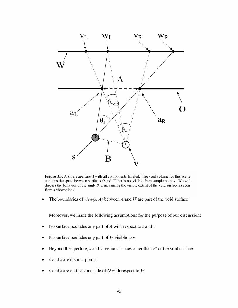
95

• The boundaries of view(s, A) between A and W are part of the void surface

Moreover, we make the following assumptions for the purpose of our discussion:

• No surface occludes any part of A with respect to s and v

• No surface occludes any part of W visible to s

• Beyond the aperture, s and v see no surfaces other than W or the void surface

• v and s are distinct points

• v and s are on the same side of O with respect to W

wR vRwLvL

aRaL

B

A

s v

θs

θv

θvoid

W

O

Figure 3.5: A single aperture A with all components labeled. The void volume for this scene contains the space between surfaces O and W that is not visible from sample point s. We will discuss the behavior of the angle θvoid measuring the visible extent of the void surface as seen from a viewpoint v.

96

We quantify the visibility of the void surface using the angle it subtends with

respect to the viewpoint v. We will refer to the magnitude of this angle as the visible

extent of the void surface. The visibility of the void surface will depend on the relative

placement and spacing of v and s. This relation has two components:

• Whether one of s or v is contained in the other�s view of A, and

• How far apart s and v are compared to the (projected) extent of A.

We will first examine the behavior of the void surface for a single aperture, then

discuss its properties in an environment with many apertures and complex occlusion.

3.2.2.1 Classifying the visibility of the void surface The visibility of the void surface in a single sample can be characterized

according to the relative positions of a sample point s and a viewpoint v. In this section

we enumerate the four different situations that can arise.

97

3.2.2.1.1 Case 1: s ∈ view(v, A) (Figure. 3.6) If the sample location s is located between v and A, the portion of view(v, A)

beyond A is completely contained within view(s, A) as shown in Figure 3.7. We then

have

vs θθ > and θvoid=0 (1)

Figure 3.6: Visibility of the void surface, case 1. view(v, A) is completely contained within view(s, A).

θs

θv

wRvRwL vL

s

v

A

98

3.2.2.1.2 Case 2: v ∈ view(s, A) (Figure 3.7) If v is located inside s�s view of A, view(v, A) will extend beyond the borders of

view(s, A). The visible extent of the void surface is the sum of the angles subtended on v

by the segments of the void surface visible beyond the aperture. These two segments are

bounded by (wL, aL) and (wR, aR) in Figure 3.8.

vs θθ < and θvoid≥ sv θθ − (2)

( ) ( ) ( ) ( )

−−−⋅−

+

−−−⋅−

= −−

vavwvavw

vavwvavw

LL

LL

RR

RRvoid

11 coscosθ (3)

Figure 3.7: Visibility of the void surface, case 2. If v is contained within view(s, A), v will see the void surface where its view frustum extends beyond the sampled data.

aL aR θv

θs

vRwRvL wL

s

v

A

99

3.2.2.1.3 Case 3: (view(v, A) ∩ view(s, A)) broadens beyond A (Fig. 3.8) Construct a line M parallel to (wL � s) that passes through aR. If v and s lie on the

same side of M, then the overlap between view(v, A) and view(s, A) does not grow

narrower when moving beyond A. The visible extent of the void surface is then the angle

subtended by the segment (wL, aL):

( ) ( )

−−−⋅−

= −

vavwvavw

LL

LLvoid

1cosθ (4)

if v is to the right of s. Replace wL and aL with wR and aR if s is to the right of v. Figure 3.9 shows an example.

Figure 3.8: Visibility of the void surface, case 3. The intersection of view(v, A) and view(s, A) broadens beyond the aperture.

B

θs θv

wRvRwLvL

aL aR

100

3.2.2.1.4 Case 4: view(v, A) ∩ view(s, A) narrows beyond A (Fig. 3.9) Construct a line L passing through wL and aR. If L falls between s and v, then the

overlap between view(v, A) and view(s, A) grows narrower when moving beyond A. In

this situation it is possible for the void surface to cover all of θv. See Figure 3.9 for

details. The following is true of θvoid, assuming that v is to the right of s:

When v lies to the right of line L, vR lies to the left of wL and no part of W is

visible to both s and v. Therefore vvoid θθ = . If v lies to the left of line L, the intersection

of view(v, A) and view(s, A) on W is non-empty and

( ) ( )

−−−⋅−

= −

vavwvavw

LL

LLvoid

1cosθ (5)

As above, replace wL and aR with wR and aL if s is to the right of v.

Figure 3.9: Visibility of the void surface, case 4. The intersection of view(v, A) and view(s, A) narrows beyond the aperture. If the viewpoint is on the opposite side of line L from the sample point, the void surface will subtend all of view(v, A).

B

θs

θv

L

wRvRwLvL

aLaR

101

3.2.2.2 Summary of regions of behavior Figure 3.10 shows the regions corresponding to the different visibility patterns of

the void surface. Given a sample location s, placing a viewpoint v in one of the

numbered regions will give rise to one of the corresponding case labeled above. The

unlabeled dark gray regions are those parts of Case 4 where the void surface subtends all

of view(v, A). We observe that side-to-side translation with respect to an aperture will

tend to increase the visibility of the void surface, and that as a viewpoint moves farther

away from a sample location, the void surface covers more and more of the aperture.

This suggests that new sample locations will contribute the most information if they are

placed far from existing samples so that the void surface will cover as many apertures as

possible.

Figure 3.10: Behavior of the void surface as a function of the placement of a viewpoint and a sample location. The numbered regions correspond to the behavior observed when the viewpoint falls within each.

2

1

3344

S

A

102

3.2.2.3 Behavior of apertures in complex environments The focus of the previous section was the behavior of a single aperture, a single

sample location, and a single viewpoint. In practice such simple situations rarely occur.

Each object in an environment can generate an aperture along each of its visible

boundaries that can possibly occlude another object. In complex scenes, this can result in

views with tens or hundreds of apertures. Figure 3.11 shows a particularly intricate case.

Qualitatively, the presence of a surface T in an environment can affect the void surface in

the following ways:

1. If T occludes an endpoint a of A with respect to s, the segment of the

void surface beginning at a is removed.

Since this operation reduces the extent of the void surface itself, it will

definitely not increase its visible extent with respect to a viewpoint v.

2. If an endpoint t of T is visible to s, a new segment X of the void surface

Figure 3.11: A scene with many interacting occluders. Many occlusion and disocclusion events occur in a small view volume, causing the explicit computation and management of apertures to be impractical.

103

is introduced beginning at point t along the line through s and t.

By introducing new segments of the void surface, this operation has the

potential to increase its visible extent. In particular, any portion of X that

extends beyond the umbra of T (the region of space immediately behind T

invisible to both s and v) is potentially visible from v.

These two situations can both occur at the same time: see Figure 3.12 for an

example. Moreover, the exact changes to the visibility of the void surface are scene- and

viewpoint-dependent. Combining the behavior of many individual apertures over a

viewing region V in a complex environment amounts to computing the exact visibility of

the void surface with respect to V. At present, the algorithms that would support such an

approach have prohibitively high computational complexity. We will propose heuristics

for placing new sample locations by taking into account the qualitative behavior of the

void surface in order to avoid the computational expense and complexity of maintaining

the visibility structures necessary for an exact characterization. The analysis in this

Figure 3.12: Introducing new surfaces can increase the visibility of the void surface. The introduction of a surface T that partially occludes an aperture A from a sample point s eliminates segment Y of the void surface part of the void surface and introduces a new segment X. The net effect is to increase the visibility of the void surface from viewpoint v.

v s

T

X

v s

A

(a) (b)

Y

104

section suggests that a new sample location that is far away from existing samples will

tend to see more of the void surface than one that is close to existing samples.

3.2.3 Reconstruction errors due to finite sampling The reconstruction errors discussed in Section 3.2.1 arose through a lack of

information about surfaces that should be visible but were not sampled. In our discussion

of such visibility errors we assumed that samples of the environment were acquired at

infinite resolution. In practice, the finite resolution of the sensor introduces two more

types of error in the reconstruction. First, a sample will omit or misrepresent high-

frequency components of the plenoptic function. This can cause potentially visible

surfaces to be absent from the reconstruction, or perhaps present but incorrect due to

aliasing. Second, the individual elements in a sample are themselves acquired with

limited precision. This affects the accuracy with which sharp edges and smooth curves

can be reconstructed. In this section we will describe these errors and illustrate situations

in which they occur.

105

3.2.3.1 Errors due to sampling frequency Samples of the environment can be interpreted as sets of samples of the plenoptic

function of an environment. Recall that if we ignore time and wavelength, the plenoptic

function can be parameterized over the 3-dimensional space of viewpoints and the 2

dimensions of view directions, mapping a viewpoint and a view direction to an intensity

value:

RSRxL →× 23:),,( φθ (6) The plenoptic function is not inherently band-limited. As a result, sampling it

with any finite resolution can fail to capture high-frequency components. When these

components are the edges of a surface, the resulting error often takes the form of jaggies

or stair-step artifacts. In environments where an entire object falls within the solid angle

subtended by a single pixel, a sampling error can cause that object to be completely

absent from the reconstruction. We will use a one-dimensional example as an illustration.

Figure 3.13: Pixel numbering in one face of a hypothetical 1D sample. We are interested in the sampling frequency at different points along the sample as a function of resolution. The point corresponding to a pixel p is taken to be the corner of that pixel closest to the center of the image. For example, the sample point for pixel 0 is directly in front of the gray viewpoint.

r/2 � 3 2 1 0 1 2 3 � r/2 0

106

Consider a 2D environment in which a sample (a panoramic environment map) is

represented as a square surrounding some viewpoint. Each face of the square is divided

into some number of pixels numbered as shown in Figure 3.13. Each pixel in a face

contains a single intensity value (sampled from the plenoptic function) plus a depth value.

This arrangement results in different pixels subtending different angles with respect to the

sample location. We choose it because it is exactly analogous to a cube environment map

in three dimensions. This allows us to describe the variation in the resolution of a sample

at different locations within the environment map, and thus establish bounds on the

minimum projected size of a surface in order to guarantee its visibility.

Using the pixel numbering from Figure 3.13, we can compute the angle subtended

by a pixel p as follows:

−

+

= −−

2

tan

2

1tan 11

rp

rp

pθ (7)

where r is the resolution of each side of the environment map and pixels are numbered

0 � p p+1 � r/2

Figure 3.14: Finding the angle subtended by pixel p. We want to find the angle between the two black lines, one of which passes through the sample point for pixel p and the other of which passes through the sample point for pixel p+1.

107

from the center of each side outward as shown in Figure 3.13. This corresponds to the

angle between the lines from the viewpoint through the sample points for pixels p and

p+1 in a situation where the line through pixel r/2 makes a 45-degree angle with the line

through pixel 0. See Figure 3.14. We can find the maximum variation in the angles

subtended by different pixels as follows:

)()(limlim

2

0

2

0

rr

rr angle

angleθθ

θθ

∞→∞→= (8)

−−

−

=

−−

−−

∞→∞→

2

12tan

2

2tan

2

0tan

2

1tan

limlim

11

11

2

0

r

r

r

r

rr

rr

r θθ (9)

( )

−−

=

−−

−

∞→∞→

2

12tan1tan

2

1tan

limlim

11

1

2

0

r

r

r

rr

r θθ (10)

Applying L�Hôpital�s rule, we then have:

−+

−

−

+

−

∞→

221

22

2211

1)1(tan

221

1

lim

rr

rr

r (11)

108

After simplification and another application of L�Hopital�s rule this becomes:

2

2

41

2212lim

r

rrr

+

+−

∞→, which is equal to 2. (12)

The angle subtended by a pixel at the center of a face is thus at most twice that of

a pixel at the corners of the environment map. Correspondingly, the sampling frequency

at the center of a face of the environment map is at least half of its value at the corners.

We can use this result to make statements about what surfaces can be

reconstructed from a given viewpoint. Again, we consider a two-dimensional example

with a one-dimensional space of viewpoints. The extension to solid angles and a 2D view

sphere is straightforward.

Consider the depth values acquired during the process of generating a sample as a

1D signal [ ) Rf →π2,0: . Each of the four faces of the environment map is divided into

r pixels, each of which contains one sampled depth value. As described above, the

sample elements are not spaced evenly in θ. The sampling theorem states that sampling a

signal f at a frequency λ

ν 1= will allow the reconstruction of those components of f with

frequencies no greater than 2ν . In the 1D signal of depth values, the sampling interval λ

corresponds to the pixel spacing θp described above. We make the conservative

simplifying assumption that θp = θ0 across an entire face of the sample. As a result, we

can reconstruct those parts of the depth signal that exist at frequencies lower than 2ν ,

109

which is equivalent to the assertion that a surface must subtend at least two pixels in a

sample in order to be present in the reconstruction.

Given these results, it is possible to state bounds on the spatial extent of a surface

S in order for it to be properly sampled in one face of a sample. Suppose that surface S is

visible around pixel p in a sample. Since pixel p subtends angle θp, the visible portion of

S must subtend at least 2 θp. Let d be the distance between the sample location and S and

ρ be the angle between S and an eye ray from the sample location. The following

equation must hold in order for the surface S to subtend at least two pixels and thus be

adequately sampled for reconstruction:

Length(visible portion of S) ≥ ρθ cos2 pd (13)

This suggests that very small surfaces in the far field may not be adequately

sampled via rasterization, especially in large environments where the viewpoint can be

far away from such surfaces. We can consider this as providing a lower bound on the

sizes of surfaces that a rasterization-based visibility algorithm cares about. Such an

algorithm will be used as part of our incremental sampling scheme.

3.2.3.2 Errors due to limited precision in samples Even when a surface is sufficiently well sampled for reconstruction, the limited

precision and resolution of samples will introduce errors in the reconstruction. These

errors arise from the use of single point samples to approximate a surface over the entire

angle subtended by each pixel. These errors show up at the edges of a surface, where an

entire square pixel will be used to represent a surface fragment that probably subtends

only a small portion of the corresponding solid angle.

110

The behavior of such error is determined by the rasterization process for a triangle.

Moreover, only the pixels intersected by the edges of the triangle can introduce errors. If

a pixel is wholly in the interior, it will definitely be part of the scan-converted triangle

and is completely covered by that triangle. Pixels along triangle boundaries can

introduce two kinds of errors: underestimating triangle area, when an edge intersects a

pixel that is not illuminated; and overestimating triangle area, when some fraction of an

illuminated pixel is outside the triangle.

The OpenGL specification [Segal and Akeley 2002] states that lines (including

edges of polygons) should be scan-converted using the diamond exit algorithm. This

algorithm operates by placing a unit-height diamond inside each pixel. A pixel is

illuminated if and only if the line being rasterized leaves its corresponding diamond. As

a result, the error produced by rasterizing any given line depends in large part on the

parameters of the line, as demonstrated in Figure 3.15. Moreover, the error in the

rasterized area of a single triangle T can be affected by the error in the rasterized area of

triangles that partially occlude T. Finally, the diamond exit rule is not an absolute

requirement: the OpenGL specification allows different algorithms for rasterization

subject to certain constraints. A conservative approach to management of rasterization

error would be to count the number of pixels on the boundary of the rasterized void

surface and add their area again into the solid-angle estimate. In practice, we assume that

the various factors causing increase or decrease of the error will tend to balance one

another out and forego any explicit error compensation. To reduce the impact of this

error, we will evaluate the quantitative visibility of a surface over the union of all visible

segments of that surface instead of considering each individual segment separately.

111

Whereas this reduces the precision with which we can perform visibility computations, it

is not a critical obstacle since our sampling algorithm will evaluate the aggregate

visibility of the void surface from a point instead of measuring its individual visible

segments.

3.3 Problems with point-sampled visibility

In this section we argue that it is difficult to guarantee that a set of environment

scans contains all potentially visible surfaces in an environment E given a navigable

region NR. We conjecture that such a guarantee requires either prior knowledge of the

potentially visible set or exact region-based visibility information from NR onto E.

In situations where the primitives in the environment are available a priori,

[Stuerzlinger 1999] presents a method for computing a near-optimal set of viewpoints

given a two-dimensional navigable region based on hierarchical visibility calculations in

Figure 3.15: Rasterization error. Two lines are shown passing through some set of five adjacent pixels. According to the diamond exit rule, all five pixels will be illuminated for each line. If the interior of some notional polygon lies below each line, a different amount of error in that polygon�s rasterized area will be incurred depending on their relative placement. In this figure, the error for each case is shaded in dark gray.

(a)

(b)

112

the environment. Although there is no guarantee offered that every potentially visible

surface will be captured, the authors present empirical evidence of the convergence of

their method. Our approach, however, is intended to operate under conditions where

surfaces may only be discovered by examining samples. We claim that under such

conditions it is difficult to guarantee a complete sampling of potentially visible surfaces

without exact region-based visibility. We conjecture that such a guarantee is in fact

impossible to provide, although a proof is beyond the scope of this dissertation. If

samples are acquired at any finite resolution this assertion holds immediately. Even

when samples are acquired at infinite resolution, we will describe environments that can

be constructed to require an arbitrarily large number of samples in order to capture all

potentially visible surfaces.

3.3.1 Uncertainty in Finite-Resolution Sampling Any point-sampled representation of an environment, whether rasterized from

synthetic data or acquired from the real world using a range scanner or other imaging

device, approximates the set of visible primitives over some solid angle using a single

sampled point on a single surface. This is true even in the presence of anti-aliasing: even

though the range sample may be a combination of several taken at higher sampling

frequencies, that one sample still represents the entire pixel. As a result, point-sampled

representations cannot distinguish between an environment containing a single large,

continuous surface and one containing a single tiny surface patch for each eye ray. See

Figure 3.16 for an illustration. Adding more samples does not remove the problem. As

long as samples are acquired at finite resolution, there will be a finite number of eye rays

113

and it remains possible to construct an almost-totally-empty environment that nonetheless

appears continuous in each scan.

3.3.2 Difficult cases for exact point-based sampling The previous argument relied on the presence of aliasing in a sample of the

plenoptic function with a fixed viewpoint. In this section we discuss environments where

many samples are required to capture all visible surfaces even when those samples are

taken with infinite resolution. We make the following assumptions in this discussion:

1. The geometry of the world can be sampled but not examined directly. We

only know about the portions of surfaces visible in samples.

2. Samples have infinite resolution: there is no aliasing.

3. An exact representation of the void surface can be computed from a set of

samples.

Figure 3.16: A finite-resolution sample taken from the gray point cannot distinguish between these two environments since visible surfaces are only sampled at discrete points. The second environment is enclosed by surface that is not intersected by any view ray and is thus invisible in the panoramic sample. The line segments that obstruct the view rays can be made arbitrarily thin without changing this result.

114

4. Region-based visibility techniques are prohibitively expensive and cannot be

employed.

5. New sample locations will be computed by constructing the Voronoi diagram

of the existing sample locations, then choosing the Voronoi vertex within the

navigable region where the void surface is most visible. A similar argument

can be constructed for other methods.

Consider the environment shown in Figure 3.17. The navigable region is one-

dimensional for the purposes of this example. The aperture is an opening in an object

with depth dA. In previous examples, the surface containing the aperture has been

infinitely thin. The sampling process begins with two samples acquired at the extremes

of NR. We will describe an aperture configuration for a set of environment scans R1..Rk

Figure 3.17: Configuration of an environment in which a finite number of samples acquired using Voronoi-based sampling will fail to acquire all potentially visible surfaces. Only samples taken from viewpoints within VNR will be able to see through the far side of the aperture. Given a number of samples S1..SN, an aperture A can be chosen with depth dA and width W so that no sample S falls within VNR.

ds

S2

VL VR

VNR

NR

dA

S1

A

115

taken from sample locations S1..SN that contains potentially visible surfaces not imaged

in any scan.

Step 1: Find the extent of the viewing region V within NR that can see the far side of A.

The boundaries of V occur where two opposite corners of A (near left / far right,

near right / far left) coincide during projection. Construct lines VL and VR as shown in

Figure 3.18. The open set V formed by the intersection of the half-plane to the right of

VL and the half-plane to the left of VR contains only points that can see through A. The

width of the intersection of V with NR is computed from the configuration of the aperture

and the standoff distance:

2

2A

As

NR d

ddANRVV

+=∩= (14)

If no sample location Si falls within VNR then any primitives beyond A will

remain unsampled. We will now express |A| in terms of the number of samples k, the

depth DA of the aperture, and the distance Ds between NR and the surface containing A.

Sample locations S3..Sk will be chosen using the Voronoi diagram of existing sample

locations as described above.

Step 2: Find new sample locations.

Until one of the sample locations Si can see all the way to the far side of the

aperture, the void surface will completely obstruct A. As each new sample Ri adds

information about the environment, the void surface is pushed farther back inside A as

shown in Figure 3.19. It follows that a sampling algorithm based on the visibility of the

116

void surface will choose the candidate viewpoint where A subtends the largest fraction of

the view. This yields a sampling pattern (shown in Figure 3.18) similar to a binary search.

Figure 3.19: The introduction of a new sample location in part (b) can push the void surface farther back into the aperture without eliminating it entirely.

View region (1D)

Void volume Void volume

New sample

(a) (b)

Figure 3.18: Binary-search sampling pattern generated by Voronoi-based sampling. An aperture configuration can be chosen for any finite number of samples that guarantees that no sample will see through to the far side of the aperture Only the part of the navigable region between the two arrows will be able to see surfaces on the far side. .

S1 S2S3 S4NR

117

Step 3: Find the maximum width of the aperture.

After acquiring k samples, the size of the interval of NR containing VNR has been

reduced to 22 −k

NR. This yields the following inequality:

22 −< kNR

NRV (15)

By incorporating Equation 14 we see that

222

2−<

+

kA

As NR

d

ddA (16)

122 −<

+ k

AAs

dNRddA (17)

( )122

−

+

<kA

s

A

dd

dNRA (18)

This yields the maximum width |A| of an aperture whose far side will remain

invisible to each sample R1..Rk. In order to miss every sample location, VNR must fit

completely within the region bounded by Sk-1 and Sk. This may be accomplished by

centering A above the point 2

1 kk SS +− . However, a new sample Sk+1 will capture the

surfaces visible through this aperture. To understand why, consider the following

argument:

In this one-dimensional navigable region, the Voronoi diagram of the sample

locations Si consists of the midpoints of each adjacent pair of sample locations. One

point P in the Voronoi diagram will fall between Sk-1 and Sk, which (by construction) is

118

directly below the center of the aperture. Since no sample has yet seen through to any

surface beyond A, the aperture is entirely obstructed by the void surface. Moreover,

since the walls of the aperture do not occlude any part of the void surface from P, it will

be chosen as the next sample location. Even if some other Voronoi vertex Q can see the

entire void surface, its visible extent will be less than that at P because of Q�s greater

distance from the aperture. Since A is centered directly above P, nothing occludes P�s

view of the far side of the aperture. Therefore, the sample acquired from P will see

through A to capture surfaces on the far side of the aperture.

We have now described the configuration of an environment containing a single

aperture A that will contain potentially visible surfaces not visible from any of k sample

locations where k ≥ 2. These sample locations are chosen from the vertices of the

Voronoi diagram of existing sample points. Although sample k+1 will capture at least

some of these surfaces, it is possible to construct another environment where those k+1

samples will miss some potentially visible surfaces. Although we believe such

environments exist for any sampling algorithm guided by maximization (or minimization)

of an objective function without explicitly constructing the visibility volume of the void

surface, such an argument is beyond the scope of this dissertation. We draw two

conclusions that will support the algorithm presented in the next section:

1. Algorithms based on a discrete set of samples of an environment

may not be able to guarantee complete capture of all visible surfaces

without more information than is present in the samples alone.

119

2. The maximum severity of visibility artifacts due to unsampled

surfaces decreases according to the distance between nearby sample

points.

3.4 An approximate Voronoi-based best-next-view algorithm

In spite of the difficulty of guaranteeing complete capture of all visible surfaces, it

is possible to construct approximate algorithms that perform well in many environments.

In this section we describe a best-next-view algorithm that chooses new sample locations

based on the Voronoi diagram of all sample locations so far. This algorithm is guided by

the following assertions discussed in previous sections:

1. The visibility of the void surface tends to increase as a view location

moves farther from a sample location.

2. Limits on the maximum distance between a viewpoint and nearby

sample points can decrease the severity of visibility artifacts in the

reconstruction.

3. The visible area of a surface can be approximated by rasterizing it

and adding the areas of each pixel illuminated. This estimate is

subject to error along the boundaries of the visible region.

Our algorithm is presented as an incremental search for the best next view of an

environment. We begin with a set of initial sample locations that are used to build a

rough reconstruction of the environment. Given a set of sample locations, we use the

Voronoi diagram with these locations as sites to construct a set of candidate locations for

the best next view. We choose one of these locations by evaluating an objective function

120

at each candidate viewpoint. The value of this objective function at a point is defined as

the approximate solid angle subtended by the void surface. Finally, we describe

termination criteria for the incremental sampling process based on the values of the

objective function.

3.4.1 Choosing initial sample locations In many architectural environments, visibility changes smoothly: the closer two

viewpoints are to one another, the more coherence exists in their potentially visible sets.

Conversely, we expect that the PVS for two viewpoints will diverge as the viewpoints are

moved farther apart. Since we have assumed that nothing is known about the

environment before the first sample is acquired, the best we can do is to choose points

spaced as widely as possible within the navigable region. If this assumption is relaxed, it

might be possible to find reasonable initial sample points by computing the intersection

of the medial axis of free space in the environment with the navigable region and

choosing points at maximum distance from any primitives. We avoid such an approach

in order to preserve the ability to apply our methods to real-world environments.

Moreover, exact computation of the medial axis is difficult to implement robustly.

Our algorithm captures parts of a 3D environment visible from locations within a

2D navigable region. The reconstruction process typically begins with four or five

samples of the environment. Two samples are required at minimum to guarantee a well-

defined Voronoi diagram for estimation of new viewpoints. In practice we usually use

four scans, one from each corner of the navigable region, plus an optional fifth scan taken

from the center. More environment scans may be added at the midpoints of the sides of

the navigable region. In practice, however, these additional scans usually convey little

121

added benefit unless the visible environment is known ahead of time to be exceptionally

complex.

3.4.2 Objective Function: angle subtended by the void surface The driving application of interactive walkthrough of synthetic environments

dictates the major concerns of the sampling process and thus the nature of the objective

function. Since artifacts in the reconstruction are due mainly to exposure of the void

surface, the value of the objective function should increase near viewpoints where the

void surface subtends a large portion of the field of view. Moreover, we are not

concerned with sampling density, as the samples acquired in this phase will only be used

to reconstruct the far field. The user is not expected to approach closely enough to see

significant artifacts caused by insufficient sampling resolution. Finally, since we are

working with synthetic environments, the only errors in the per-pixel depth estimates are

due to the limited floating point precision of the depth buffer. It is not necessary to

sample all visible objects from within a certain cone surrounding the surface normal in

order to ensure accurate capture of surface properties (including depth, where applicable).

We have chosen to use the solid angle subtended by the void surface as the value

of the objective function at a point. Given the ability to construct the void surface for a

single sample, this angle acts as a reasonable, conservative estimate of the wrongness of a

view. Since it does not attempt to compare the reconstruction against the original images,

this measure does not suffer from cases where a numerical comparison such as mean

squared error is a poor predictor of visual similarity. Moreover, the construction of the

void surface can be performed entirely within the sampled data without need to refer to

the original environment. This suggests that it will remain useful as an error measure in

122

environments where access to the original primitives is inconvenient or even impossible.

At the same time, using the angle subtended by the void surface may overestimate the

severity of artifacts in two ways. First, as an aggregate measure it has no notion of the

individual errors in a view: one thousand single-pixel errors which might very well be

invisible in a 1.5-million-pixel panorama are considered just as severe as a large, 1000-

pixel patch in the center of one face of the panorama. Second, there is no notion of

minimum perceptible error. Reconstruction errors such as mistakenly covering over

concavities in distant objects may not be perceptible if the objects are far away and the

concavities relatively small; however, the angle-measure criterion will weight these

errors as heavily as others that involve radical changes in color or occlusion.

Finding viewpoints where the void surface subtends the largest fraction of the

view will guide the sampling algorithm toward locations where a new sample of the

environment will contribute more information to the reconstruction. In this section we

describe an implicit representation of the void surface along with a graphics hardware-

accelerated algorithm for computing its visible extent with respect to any point in the

environment.

3.4.2.1 Rendering the void surface In order to evaluate the objective function from a given point P in an environment,

we must first render the void surface as seen from P and then compute its visible extent.

Recall that the void surface forms the border between visible space and invisible space:

any point on the void surface or in the volume behind it is not sampled at all in any

sample. As such, the void volume for an environment consists of space in the

intersection of the void volumes for each individual scan. We can construct the void

123

surface for an individual sample by classifying all potential edges in a dense mesh

constructed over the elements in that sample as valid edges (belonging to an existing

surface) or skin edges (corresponding to no surface in the environment). Any polygon in

the dense mesh that contains at least one skin edge is part of the void surface. The chief

advantage of this polygonal representation is that the graphics hardware can resolve its

visibility at little extra cost by rendering it on top of a reconstruction of the environment.

However, this approach is subject to the sampled nature of the frame buffer and can only

compute visibility up to a certain resolution.

3.4.2.1.1 Constructing the void surface for a single sample In order to construct a polygonal representation of the void surface, we classify the

edges between each pixel in each sample and its eight neighbors according to whether or

not that edge is present in the original environment. This classification is equivalent to

detecting and removing skins. Recall that a skin is a surface in a textured depth mesh that

is not present in the original environment. Skins arise when an edge is mistakenly

created between two sample elements that belong to different surfaces or are separated by

a significant depth discontinuity. A single sample does not contain enough information

to distinguish between skins and legitimate surfaces in certain borderline (but relatively

common) cases. However, this information is present in a collection of samples that look

on the same environment. The determining criterion for identifying a point as belonging

to a skin is whether a different sample sees past the point (and hence the potential skin) to

a more distant region of the environment. This test is potentially an expensive operation:

in the worst case, it might be necessary to test every sample in a group. In order to

reduce this expense, the multiple-source skin test is used only after simpler, single-

124

source-image heuristics have been exhausted. The complete skin predicate for an edge E

= (v1, v2) uses the following heuristics in order:

1. If either v1 or v2 is at maximum depth, the edge is a skin. (Figure 3.20)

2. If the angle between E and the ray from the sample location through the

midpoint of E is less than ε = 10-6 degrees (chosen arbitrarily), the edge is a

skin. (Figure 3.21)

3. For each sample location Si, construct a ray R from Si through the midpoint of

E. If the first intersection between R and a surface visible from point Si in is

beyond the midpoint of E, the edge is a skin. (Figure 3.22)

We compute the adjacency for each of the 8 neighbors of each pixel of each face

of each sample. Since adjacency is a symmetric property (that is, pixel A is adjacent to

pixel B if and only if pixel B is adjacent to pixel A), it is only necessary to examine half

of the neighbors of each pixel to find the complete adjacency map. Pseudocode for the

entire skin test is given in Appendix A.

125

Figure 3.21: Skin detection via angle with eye ray. If a proposed edge is within a threshold angle ε of being parallel with the ray from the viewpoint through the edge�s midpoint, that edge is classified as a skin.

Object

Viewpoint

Eye ray

Potential skin edge E

α

Figure 3.20: Skin detection via background heuristic. The dashed line is identified as a skin because one of its endpoints is at maximum depth and hence not part of any valid object.

Object

Viewpoint

Eye ray

Potential skin

126

3.4.2.1.2 Using graphics hardware to visualize the global void surface Once we have constructed a set of triangles forming the void surface for each

sample, we use the graphics hardware to combine the individual surfaces into a view of

the global void surface. If a given pixel in a particular view is covered by the void

surface for every different sample, we can conclude that the surface that should be visible

at that pixel is not present in any sample. Therefore, that pixel shows the void surface.

The algorithm to identify these pixels is as follows:

1. Initialize each pixel in the stencil buffer to zero.

2. For each sample R:

3. Render the current reconstruction of the environment using all samples.

4. Render the void surface for sample R.

Eye ray

Potential skin edge E

Object

Viewpoint 1

2

Midpoint of potential skin

2

Figure 3.22: Skin detection using multiple source images. If a second sample (2) sees through a potential skin edge to more distant surfaces, that edge is classified as a skin.

127

5. Increment the stencil buffer at all locations where the void surface is

visible.

6. After rendering the void surface for each sample, pixels in the stencil

buffer whose value is equal to the number of samples belong to the void

surface.

Figure 3.23 illustrates this approach.

128

(a) (b)

(c) (d)

(e)

Figure 3.23: Computing the visible extent of the void surface. This figure shows an example environment with two samples. The sample locations are shown as black dots. Parts (a) and (b) show the segments of the void surface for each sample. Parts (c), (d), and (e) illustrate the evaluation of the visible extent of the void surface with respect to a particular viewpoint P (the gray dot). For each sample, we render a panorama from P containing the current reconstruction (using information from all samples) and the void surface for exactly one sample. The black arc on the circle surrounding the viewpoint illustrates the angle subtended by the void surface for each sample in turn. The visible extent of the global void surface, shown in (e), is computed as the intersection of the visible extents of the void surface for each sample as shown in (c) and (d).

129

3.4.2.2 Estimating Solid Angles The solid angle subtended by the visible portion of the void surface can be

estimated as the sum of the solid angles subtended by its component pixels. This can be

computed by iterating over the pixels identified in the procedure above and maintaining a

sum of the solid angle subtended by each one. The solid angle for a pixel is computed by

treating it as a spherical polygon with interior angles θ1..θ4 and applying the following

formula for the area (see Figure 3.24):

( )πθ 21

−−

= ∑

=

narean

ii (19)

3.4.2.3 Errors in the estimated extent of the void surface By using the graphics hardware to estimate the visible area of the void surface we

incur approximation errors due to the sampling process inherent in rasterization. These

errors are exactly the same as those described in section 3.2.3. As before, we assume that

the magnitude of the error is small enough to ignore. If a more precise result is obtained,

Figure 3.24: Area of a spherical polygon. Given a convex spherical polygon with N vertices and internal angles θ1..θN, its area in steradians is equal to the sum of the internal angles minus (n - 2)π.

θ1

θ2θ3

θ4

θ5

θ6

θ7

130

it will usually be less expensive and error-prone to render the void surface at a higher

resolution than to resort to exact computation of the visible void surface.

3.4.2.4 Finding the best next view The next component of the best-next-view algorithm is a method to construct

points to be used as the locations for new environment scans. Such candidate viewpoints

are chosen in locations where the reconstruction is expected to show significant error.

After evaluating the objective function at each candidate viewpoint, one point will be

chosen as the sample location for a new environment scan. Ideally, this point should be

the best next view of the environment, where a sample will remove as much of the

(visible) void volume as possible. The search process can be stated formally as follows:

Given a region N and an objective function G, find point p such that

)()(:,: sGpGpsNsNp ≥≠∈∀∈ (20)

In a complex environment, locating the ideal best next viewpoint p is difficult. In

order to be certain of finding the location where the objective function attains its global

maximum, it might well be necessary to decompose space into view regions similar to

those in the aspect graph or the visibility complex. Such approaches are prohibitively

expensive in practice. Systems such as the one presented in [Conolly 1985] search a

regularly spaced grid of discrete points to locate a good location for the next view. We

follow [Banta et al. 1993] in searching a limited set of candidate viewpoints c1, c2, c3 �

cn believed to be good candidates for the best next view. We hypothesize that depending

131

on the choice of candidate viewpoints, this approach can give similar benefits to a brute-

force search with considerably reduced computational cost.

3.4.2.5 Generating Candidate Viewpoints Candidate viewpoints should be chosen in locations where a sample may be

expected to contribute a large amount of (non-redundant) information to the

reconstruction. Computing this contribution exactly requires knowledge of the primitives

that would become newly visible: since these primitives are hidden inside the void

volume, we must base our decisions on the behavior of the void surface. Moreover, in

reconstructions with complex occlusion, the visibility of the void surface is not always

easy to predict. Our method for generating the candidate points ci for the best next view

is based on two assumptions.

Our first assumption is that the visible extent of the void surface is a reasonable

approximation for the amount of information that will be added by a new sample. When

we acquire a sample, we assume that the sample elements are evenly distributed across

the field of view. Although there is some variation in the sample density (as discussed in

Section 3.2.3.1), we can conservatively assume that the sample spacing is no coarser than

in the center of each face of the sample. A region that projects to a small area of the scan

cube will therefore receive only a few samples regardless of the number of primitives it

may contain. More information is added to the reconstruction by sampling a large area of

simple primitives (resulting in many non-redundant range samples) than by taking fewer

samples of very densely spaced, detailed primitives.

Our second assumption is that the extent of the void surface will tend to grow

with increasing distance from sample locations. This suggests that good candidate

132

viewpoints can be found in those areas of the navigable region farthest from any existing

sample location.

We generate candidate locations for the best next view as follows. Suppose we

have already acquired N samples of the environment from locations P1, P2, P3, � , PN.

To find points as far from any Pi as possible, we construct the 2D Voronoi diagram of the

previous sample locations. The vertices and edges of the Voronoi diagram contain

Cj

Pi

N

Figure 3.25: Candidate locations Cj (squares) for the best next view are chosen from the Voronoi diagram (dashed lines) of the existing sample locations Pi (circles). The candidate points consist of the vertices of the Voronoi diagram that fall within the navigable region N as well as the intersections of any Voronoi edges with the boundary of N. The gray shapes outside N are objects in the potentially visible set. This example shows the initial sample locations chosen by our algorithm at the corners and center of the navigable region. All subsequent sample locations will be chosen from candidate points.

133

exactly those points that are at maximum distance from two or more sample locations.

Since the Voronoi diagram can extend beyond the navigable region, we choose the actual

candidate viewpoints C1 .. Cj by collecting all of its vertices that fall within the navigable

region and by finding the intersections between the boundary of the navigable region and

the edges of the Voronoi diagram. Figure 3.25 illustrates this approach. Figures 3.26

through 3.54 illustrate its operation in a simple 2D environment with a 1D navigable

region.

The 2D Voronoi diagram suffices in this case because the user�s motion is

assumed to lie in a plane. If the user is allowed to navigate in 3D space, we would need

to compute the Voronoi diagram in three dimensions. Algorithms to compute the 3D

Voronoi diagram of a set of points have a worst-case complexity of O(n2) in the number

of sample locations. This compares to the worst-case O(n log n) complexity of

computing the 2D Voronoi diagram. Note that we do not have to modify the objective

function in order to handle a 3D space of viewpoints. The objective function operates on

a 3D reconstruction of the environment and is defined at all points, not just the interior of

the navigable region.

We evaluate the objective function (the visible extent of the void surface) at each

candidate viewpoint Cj. The point at which the void surface subtends the largest solid

angle is chosen as the sample location for the next panoramic sample of the environment.

134

Figure 3.26: Example environment to illustrate Voronoi-based sampling. The black surfaces are the only objects in the world. The navigable region, shown as the green line at the bottom of the figure, is one-dimensional. We begin by acquiring two samples, S1 and S2, from the extremes of the navigable region. The 1D Voronoi diagram of these two sample points is the single point C1 at the midpoint of the segment joining S1 and S2.

S1 S2 C1

S1 S2 C1

Figure 3.27: Evaluating the visible extent of the void surface for a candidate point. We construct the void surface for each sample individually. Here we show the void volume (dark gray) with respect to sample S1 and the sight lines from the sample location S1 that bound the void surface. The blue region shows the part of the void surface that is visible from candidate location C1.

135

Figure 3.28: Visible extent of the void surface for sample S2 from candidate point C1.

S1 S2 C1

S1 S2 C1

Figure 3.29: Visible extent of the global void surface. We use the graphics hardware to compute the screen-space intersection of the visible portions of the void surface for each individual sample. This example shows the world-space intersection (dark blue region): the screen-space projection is simply the projection of this region onto a circle surrounding the candidate point C1. We are interested in the angle subtended by this projection, which in this case is 39 degrees. Since there is only one candidate viewpoint, it is automatically chosen as the location for the next sample.

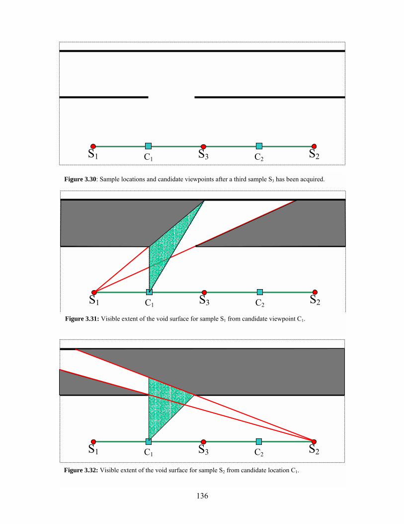
136

S1 S2 C1 S3 C2

Figure 3.30: Sample locations and candidate viewpoints after a third sample S3 has been acquired.

S1 S2 C1 S3 C2

Figure 3.31: Visible extent of the void surface for sample S1 from candidate viewpoint C1.

S1 S2 C1 S3 C2

Figure 3.32: Visible extent of the void surface for sample S2 from candidate location C1.

137

S1 S2 C1 S3 C2

Figure 3.33: Visible extent of the void surface for sample S3 from candidate location C1.

S1 S2 C1 S3 C2

Figure 3.34: Visible extent of the global void surface from candidate location C1. The global void surface (whose projection is illustrated by the dark blue region) subtends an angle of 9.2 degrees with respect to C1.

S1 S2 C1 S3 C2

Figure 3.35: Visible extent of the void surface for sample S1 from candidate location C2

138

S1 S2 C1 S3 C2

Figure 3.36: Visible extent of the void surface for sample S2 from candidate location C2

S1 S2 C1 S3 C2

Figure 3.37: Visible extent of the void surface for sample S3 from candidate location C2

S1 S2 C1 S3 C2

Figure 3.38: Visible extent of the global void surface for candidate point C2. The dark blue region subtends an angle of 2.5 degrees.

139

S1 S2 C1 S3 C3S4 C2

Figure 3.39: Sample locations and candidate points after acquisition of a new sample S4. This sample was placed at candidate point C1 from the previous stage since the visible extent of the void surface (9.2 degrees) was greater than that at C2 (2.4 degrees).

S1 S2 C1 S3 C3S4 C2

Figure 3.40: Visible extent of the void surface for sample S1 from candidate location C1

S1 S2 C1 S3 C3S4 C2

Figure 3.41: Visible extent of the void surface for sample S2 from candidate point C1.

140

S1 S2 C1 S3 C3S4 C2

Figure 3.42: Visible extent of the void surface for sample S3 from candidate location C1

S1 S2 C1 S3 C3S4 C2

Figure 3.43: Visible extent of the void surface for sample S4 from candidate point C1.

S1 S2 C1 S3 C3S4 C2

Figure 3.44: Visible extent of the global void surface from candidate point C1. The global void surface is not visible at all since the intersection of the views of the void surfaces for individual samples (particularly S1 and S4) is empty.

141

S1 S2 C1 S3 C3S4 C2

Figure 3.45: Visible extent of the void surface for sample S1 from candidate point C2.

S1 S2 C1 S3 C3S4 C2

Figure 3.46: Visible extent of the void surface for sample S2 from candidate point C2.

S1 S2 C1 S3 C3S4 C2

Figure 3.47: Visible extent of the void surface for sample S3 from candidate point C2.

142

S1 S2 C1 S3 C3S4 C2

Figure 3.48: Visible extent of the void surface for sample S4 from candidate point C2.

S1 S2 C1 S3 C3S4 C2

Figure 3.49: Visible extent of the global void surface from candidate point C1. As before, the intersection of the individual views is empty. The global void surface is not visible at all from this location.

S1 S2 C1 S3 C3S4 C2

Figure 3.50: Visible extent of the void surface for sample S1 from candidate point C3.

143

S1 S2 C1 S3 C3S4 C2

Figure 3.51: Visible extent of the void surface for sample S2 from candidate point C3.

S1 S2 C1 S3 C3S4 C2

Figure 3.52: Visible extent of the void surface for sample S3 from candidate point C3.

S1 S2 C1 S3 C3S4 C2

Figure 3.53: Visible extent of the void surface for sample S4 from candidate point C3.

144

3.4.3 Termination Criteria The goal of the incremental sampling process is to capture a set of surfaces that

approximates the potentially visible set for a view region as closely as possible.

Accordingly, an ideal termination criterion would be to continue taking samples until the

visibility of the void surface falls below some threshold value for every point in the view

region. Rather than compute this exactly, we once again make use of the assumption that

the visibility of the void surface will tend to increase with increasing distance from a

sample location. The set of visible surfaces is deemed to be �complete enough� when the

value of the objective function at every candidate viewpoint falls below some user-

specified threshold value. Common values for this threshold range from 0.5% to 2% of

the space of view directions (roughly 0.0628 to 0.264 steradians).

S1 S2 C1 S3 C3S4 C2

Figure 3.54: Visible extent of the global void surface from candidate point C3. The global void surface subtends an angle of 2.5 degrees with respect to this point. We end the example here: if we were to continue, the next sample would be acquired from candidate point C3 and the evaluation process would repeat.

145

3.5 Analysis

This section discusses the properties of the incremental Voronoi-based sampling

algorithm. As seen in Section 3.3.2, the fact that our algorithm only samples visible

surfaces at discrete points suggests that it is generally possible to construct an

environment where our method will miss some potentially visible surfaces. We claim

that this is not a fatal drawback. The Voronoi-based sampling scheme presented in this

section has been tested in synthetic CAD environments of a one-story, 261,000-polygon

house and a 52-story, 12.7-million-polygon power plant. Examples drawn from these

two environments are used to illustrate where Voronoi-based sampling performs well and

where it performs poorly.

3.5.1 Complexity of the sampling algorithm The various per-pixel operations in the incremental sampling algorithm are each

straightforward. However, they may each be invoked millions of times when adding a

new sample to the database or when evaluating the visibility error at a candidate

viewpoint. In this section we examine the computational complexity of the algorithms

driving incremental sampling in order to characterize the system�s behavior.

3.5.1.1 Per-pixel operations

3.5.1.1.1 Computing adjacency with neighboring pixels We identify skin edges using the three heuristics described in Section 3.4.2.1.1.

Their computational complexity is as follows:

1. Skin detection via the background heuristic requires the comparison of

the depth values for the two points in question and is hence O(1).

2. Skin detection via the angle of an edge with the eye ray involves a dot

product between vectors between two pairs of pixels and is also O(1).

146

3. Skin detection with multiple source images can, in the worst case,

require one test for each sample in the current reconstruction. As a result,

its complexity is O(n) in the number of samples. In practice, we rarely

observe more than 1 or 2 tests per edge when this heuristic is used.

3.5.1.1.2 Finding the visibility of the void surface We classify a pixel in a view from a particular candidate viewpoint as either

belonging to a valid surface or belonging to the void surface by rendering the current

reconstruction using all samples, then rendering the void surface for each sample and

counting how many times that surface is nearer the viewpoint than the nearest valid

surface. This operation is O(n) in the number of samples: each sample is rendered once

in the reconstruction and each sample�s void surface is rendered once to test for visibility.

3.5.1.2 High-level operations

3.5.1.2.1 Acquiring a sample Acquiring a new sample of the environment involves rendering it once for each of

the six faces of a cube environment map. The rendering process is O(n) in the number of

primitives in the environment. However, the size of the environment we wish to capture

does not change as a result of acquiring samples. As a result, we may treat this operation

as having a complexity of O(1).

3.5.1.2.2 Computing the void surface for a sample We construct the triangles belonging to the void surface within each sample by

identifying the edges belonging to skins. This identification uses the heuristics described

in the previous section applied to each pixel. Construction of the void surface therefore

has a worst-case complexity of O(n) in the size of the environment. As noted above, we

147

rarely observe O(n) behavior in the multiple-source-image heuristic: the limiting factor in

the cost of computing the void surface is usually the resolution of a sample rather than the

number of samples being used.

3.5.1.2.3 Adding a sample to the reconstruction When a new sample is added to the current reconstruction, dense polygonal

meshes are created over each face of the sample. These meshes are created using the

world-space position of each element in the sample to construct vertices. Connectivity

between vertices is taken from the the same per-pixel adjacency that we used earlier to

construct the void surface. Finding the world-space position of a single sample element

depends only on that sample�s camera information and is thus O(1). Since the number of

elements in a sample is a fixed quantity, finding the world-space positions of all elements

is likewise O(1). Moreover, we can re-use the adjacency information: we had to compute

it to construct the void surface, so we need not rebuild it here and incur no additional cost.

Finally, constructing polygons to cover a single pixel depends on the world-space

positions of that pixel and its neighbors (found in O(1) time) and the connectivity

between them (also O(1) since we can reuse the previous result). Since adding a sample

to the reconstruction consists of performing these operations on a fixed number of sample

elements, the entire process has complexity O(1).

3.5.1.2.4 Computing candidate viewpoints The candidate viewpoints are derived from the Voronoi diagram of the set of

existing sample locations. We employ Fortune�s algorithm [Fortune 1987] to compute

the Voronoi diagram of n points in O(n log n) time. In practice, this operation has

negligible cost since it is performed once for the database of samples instead of once for

148

each pixel. It typically requires a few milliseconds at most as compared with a few

minutes to evaluate the visibility error at each candidate viewpoint.

3.5.1.2.5 Evaluating visibility error at candidate viewpoints A group of n points can have a Voronoi diagram with O(n) vertices, edges, and

faces. Since the set of candidate viewpoints is derived from the vertices and edges of the

Voronoi diagram of the sample locations, we have O(n) candidate viewpoints. For each

candidate viewpoint, we evaluate the visibility error by finding the visibility of the void

surface at each pixel in a cube environment map. As described earlier, this operation

takes O(n) time in the number of samples for each pixel, giving a total complexity of

O(n2). We can accelerate this process by identifying points where the visibility error is

known to be acceptable and re-using that result as more samples are added. In practice,

this is the most expensive part of Voronoi-based sampling due to computational

complexity and the high constant factor of per-pixel processing. We simplify the

reconstruction by applying the methods described in Section 6.2.1 to remove redundant

samples before creating polygonal meshes. This dramatically reduces the cost of storing

and rendering the current reconstruction (the most expensive part of evaluating each

candidate viewpoint, often involving millions of polygons as compared with a few tens of

thousands for the void surfaces) by eliminating 70-80% of the points in new samples.

Applying a simple level-of-detail algorithm to both the surfaces in the reconstruction and

the void surface for each sample has the potential to further reduce this expense.

3.5.1.3 Overall behavior The operations described above are performed once after each sample is added to

the database. Since the complexity of finding the best next view is dominated by the

149

O(n2) cost of evaluating the visibility error, the overall cost of acquiring a set of samples

can be as bad as O(n3) in the number of samples acquired before termination. In practice,

the relatively high constant factors associated with processing each sample tend to

overwhelm the asymptotic complexity. The preprocessing times shown in Section 7.4.1

show that for the models we have tested, the cost of finding the best next view is closer to

O(n) in the number of samples, leading to an overall in-practice complexity of O(n2).

Although this behavior is model-dependent, we believe that the power plant environment

is sufficiently difficult that it represents a reasonable estimate of the performance of our

methods on difficult real-world data sets.

Finally, we note that our algorithm�s performance is a function of the (variable)

number of samples used in the reconstruction and the (high but fixed) resolution of each

sample rather than varying as a function of the number of primitives in the environment

or the number of visibility events that occur within a certain range of viewpoints. As a

result, we believe that our approach will scale to large, visually complex environments

that present difficulties for global visibility methods.

3.5.2 Where Incremental Sampling Performs Well

3.5.2.1 Characteristics of favorable environments In general, environments where the potentially visible set changes slowly and

smoothly when traversing the navigable region will be well represented after Voronoi-

based sampling. Such situations occur when most objects in the environment are far

from the navigable region or when the occlusion relations between such objects are

simple. Environments with complex geometry in the distance are often handled well: the

farther away an object is from the camera, the less horizontal parallax it will display as

150

the camera moves, which in turn reduces the potential visibility of any void volume

behind it.

3.5.2.2 Practical examples 1. House environment, living room

Figure 3.55 shows a navigable region in the living room of the house model. The

region is 1 meter square at a height of 1.5 meters. The large occluders (the green and tan

chairs, brown lamp, and green couch) near the viewpoint did not pose any major

difficulty, as they are relatively well-isolated with respect to other occluders in the

environment. An initial set of 5 samples acquired from the corners of a 1-meter-square

cell resulted in a maximum visibility error of approximately 0.07 steradians, well below

the 1% (0.1256 steradians) error threshold we used for a termination criterion.

2. Power Plant, 46th floor Figure 3.56 shows one of the simpler cases for incremental sampling in the power

plant environment. Difficult occluders such as the girders in the roof, the closely spaced

arrays of pipes, and the edges of walkways are sufficiently far away from the sample

location in most cases that their void surfaces do not become prominent from any nearby

viewpoint. A set of 9 samples reduced the maximum error to below 0.8% of the total

view (0.1 steradians). More difficult parts of the power plant can require 20 to 30

samples to achieve the same result.

151

Figure 3.55: An environment in which incremental sampling performs well. The top image shows 4 faces of a panorama taken from the center of the navigable region. Most occluders are relatively well isolated, leading to simple patterns of occlusion that are well handled by a few samples. These occluders include the couch and chairs shown in the center image (magnified from the right half of the complete panorama at top). Complex occluders including the door grille and nearby doorways to adjoining rooms shown in the center image are far enough from the viewpoint that they are not major sources of error. The bottom image shows a top-down view of the navigable region (blue square) and the sample locations (green points). The cyan lines show the ITDM dependency tree, described in Chapter 6.

152

Figure 3.56: An easy case for incremental sampling in the power plant. The T-shaped image shows all six faces of a panorama acquired from the center of the navigable region. The two smaller inset images show magnified portions from the complete panorama. Complex occluders such as the crane at far right, the roof girders shown in the top inset, and the arrays of pipes in the bottom inset are far enough from the viewpoint that they are not major sources of error. Moreover, the gaps between the pipes are small enough that at this distance they are not always rasterized, leading groups of pipes to behave as a single flat object instead of many cylinders. The bottom two images show the navigable region (blue square), sample points (green and white points), and ITDM dependency tree (cyan lines, described in Chapter 6). We began incremental sampling with 4 samples, one at each corner of the navigable region. The center of the navigable region was never found to be the best next view. This accounts for the absence of a sample there.

153

3.5.3 Where Incremental Sampling Performs Poorly

3.5.3.1 Characteristics of adverse environments Incremental Voronoi-based sampling relies on the notion that the potentially

visible set changes smoothly and slowly as the viewpoint moves. Configurations with

complex, interacting occluders close to the view volume can invalidate this assumption

by creating rapid and abrupt changes in the potentially visible set. Environments with

many thin apertures with open space on the far side are also difficult because of a lack of

overlap in the view regions of even nearby viewpoints with respect to each aperture.

Finally, environments with surfaces parallel to the camera view axis can pose minor

problems: in some cases, parts of these surfaces will be erroneously classified as skins.

Such configurations are usually easily resolved by the addition of a single sample that

sees such surfaces at a different angle of incidence.

The incremental sampling algorithm can fail entirely by vastly underestimating

visibility error in degenerate environments such as the one in Figure 3.17. However, we

have yet to encounter such a configuration in practice, even in the power plant with its

arrays of thin, closely spaced occluders.

3.5.3.2 Two practical examples 1. House model between living room and music room

Figure 3.57 shows four sides of a panorama taken from inside the house environment

on the border between two rooms. Several complex occluders generate large

segments of the void surface with respect to the view volume. From left to right,

these occluders are as follows:

154

Figure 3.57: A difficult configuration for incremental sampling inside the house environment. The top image shows four of six sides of a panoramic view taken from the initial sample location (minus the ceiling and floor, which are uniform surfaces). The center image shows a magnified view of the more difficult occluders in this environment. From left to right, these include the edges of the piano, the table and chairs in the room with the gray ceiling, the door grille, and the doorway to a neighboring room. Objects such as the green couch and brown table lamp visible in the top image introduce relatively little error for nearby viewpoints. The bottom image shows the navigable region (blue square), sample locations (green and white points), and ITDM dependency tree (cyan lines).

155

1. The green couch and table lamp in the living room at left. These

are actually the easiest of the major occluders in this scene due to

their relatively simple shapes.

2. The chairs and table to the right of the piano. Like the music stand

to their left and the door grille to the right, these objects contain

long, thin parts that create spatially large segments of the void

surface. Since the chairs and table are farther from the viewpoint,

the visible extent of the void surface they create is smaller.

3. The door grille just to the right of occluder 2. Each of the long,

thin pieces in the grille generates a segment of the void surface that

extends to the wall beyond the door. The large spatial extent of

these segments leads to correspondingly large visible extents even

though the actual void volume induced by the grille is quite small.

4. A doorway into a neighboring room. This doorway functions as a

narrow, distant aperture as described in Sections 3.2.2.1.3 and

3.2.2.1.4.

Most of the exposure errors in this scene occur around the door grille and the

doorway into the neighboring room. During an incremental sampling run that evaluated

the visibility error from a total of 45 viewpoints, the north face (the music room with the

gray ceiling) accounted for an average of 27% of the total solid angle subtended by the

void surface. The east face (containing the door grille and the doorway to the adjoining

room) accounted for 54% of the visible portion of the void surface.

156

2. Power Plant, 46th Floor Walkway

Figure 3.58 shows the six faces of a cube environment map taken from a location near

the top of the power plant. Nearby geometry has been clipped away where it intersects

the navigable region. This environment is difficult to capture completely using

incremental sampling due to the complex patterns of occlusion generated by the nearby

curved pipes. From some viewpoints, the pipes act as a single occluder that hides a large

portion of the furnace wall in the background. From other, nearby viewpoints, the pipes

act as distinct entities, and parts of the furnace wall are visible between them. Such a

configuration is shown in the larger inset image. This environment would also be

difficult for exact visibility schemes due to the interactions between objects. In particular,

the wall in the background is composed of regular arrays of thin cylindrical pipes that are

difficult to handle robustly. From this viewpoint, the furnace wall is actually

straightforward for our sampled representation, as the pipes are so close together that they

can be reasonably approximated by a flat surface.

157

Figure 3.58: A hard case for incremental sampling. The curved pipes near the viewpoint (seen in the center of the panorama and at the lower left, and in detail in the larger image) generate many visibility events in a small region. This makes it difficult to place a small number of sample locations that see all potentially visible surfaces. The navigable region and sample locations for this area are shown in Figure 3.59.

158

3.6 Summary

Incremental Voronoi-based sampling is an effective approach to capturing

synthetic environments using samples. This method constitutes an approximate solution

to the best-next-view problem: by evaluating visibility at discrete points within the

environment, it is possible to avoid the prohibitive cost of exact visibility computations.

Moreover, by operating on samples of the environment instead of the original primitives,

it is possible to sample environments where the primitives may not be available a priori

or exist in forms that are difficult to manipulate directly. By dividing the sampled

environment into visible and void volume and constructing the void surface separately for

each sample, it is possible to evaluate quickly the visibility of the void surface at any

point in the environment. Since graphics hardware is used to perform this evaluation, the

result is again an approximation to the true value; however, we have not encountered the

kinds of configurations that will induce large errors in the approximation even in the

complex environments we have explored.

Figure 3.59: Navigable region (blue square), sample locations (green/white points), and ITDM dependency tree for the difficult region of the power plant shown in Figure 3.30.

4 Spatial Video Encoding

4.1 Introduction

The geometry and image portions of textured depth meshes have sharply different

characteristics. In order to maintain a low polygon count, the geometric portion typically

contains a simplified version of the surfaces in the original samples that eliminates high-

frequency detail. However, the image portion is by definition capable of encoding high-

frequency detail including surface textures. By treating the image portions of a set of

textured depth meshes as a 3-dimensional database of images plus depth, we can apply

standard video compression techniques to create a compact representation of a database

of images derived from a group of samples.

4.1.1 Building a spatial database of images The representation for the database of impostor textures is motivated by the

properties of the initial data. This section enumerates the properties of impostor textures

and their organization based on the spatial relationships among samples.

4.1.1.1 Panoramic samples as input Impostor textures are derived from the samples acquired during the process of

capturing the environment. Six images are taken to form a cube environment map

surrounding each sample location. At a minimum, these samples include color

information for each pixel. Moreover, we assume that either depth is acquired along with

160

each sample or that it is possible to recover per-pixel depth from a group of samples as a

postprocess. The addition of camera information to each sample allows the reversal of

the 3D perspective transformation used to create the images in order to recover the world-

space locations of each individual sample element. We will use these world-space points

in the process of encoding the image component of each sample. The result of this

encoding is a compressed database of 2D images that can be used as impostor textures.

4.1.1.2 Properties of Synthetic Environments Synthetic environments often exhibit certain properties that simplify the

comparison of one impostor texture to another as well as the construction of a database of

spatially encoded video. Those properties are as follows:

1. The environment is static. All apparent motion from image to image is the

result of camera parallax.

2. Free space is transparent. No volumetric effects such as fog or distance-

attenuated color saturation are present.

In addition, we assume that the surface reflectance in the environment is diffuse

and constant over time. This allows us to handle diffuse lighting as a component of

surface texture.

Taken together, these properties suggest considerable coherence in the sets of

surfaces visible in samples acquired from viewpoints near one another. Moreover, since

all image-space motion is due to camera parallax, it will be possible to predict the

changes from one image to the next. This provides a solution to the correspondence

problem of identifying which pixels in different frames belong to the same object.

161

4.1.1.3 Operations on samples In order to detect coherence in our input samples and remove redundant data, we

must be able to compare and modify portions of samples. This chapter focuses on spatial

representations for a compressed database of 2D images, suggesting that the comparisons

and modifications should take place in image space instead of on the 3D range samples.

4.1.1.3.1 Comparing Image Data There are many possible operators for determining the degree of similarity of two

images. Roughly speaking, such operators can be classified as signal-processing

techniques or perceptual comparisons. First, a domain for comparison can be established

by treating an image as a two-dimensional signal. Under this assumption, the difference

between two images is likewise a 2D signal. Comparisons using this difference may be

quantified by methods such as the sum of squared differences (SSD) or of absolute

differences (SAD), the computation of mean squared error (MSE), or by transforming

both images into frequency space and comparing their power spectra. This sort of

comparison is often useful when trying to minimize the difference between some

compact, lossy representation and the original input data.

Perceptual measures comprise another category of comparison operations: instead

of computing any and all differences between a pair of, a perceptually based comparison

attempts to highlight only those differences that a hypothetical human observer would

notice. Such operations typically take into consideration the properties of the display

device, including lighting conditions and the observer�s distance from the screen, and

detect visible differences by passing the input images through a series of filter banks

designed to simulate portions of the human visual system. Either a signal-processing

approach or a perceptual comparison would be sufficient for our purposes. To simplify

162

implementation, image-space comparisons are implemented in this dissertation using

signal-processing techniques.

4.1.1.3.2 Modifying Image Data Once we have detected redundant information using a comparison between two

samples, we modify the input data in order to reduce or remove such duplicated

information. Removal is a trivial operation when dealing with images: since each pixel is

independent of its neighbors, it is possible to simply zero out individual pixels as they are

deemed unnecessary. Redundant samples may also be flagged with a �don�t care� value.

If images are represented using a lossy compression scheme, such a value may allow

redundant samples to be filled in with colors that will reduce the amount of information

necessary to faithfully represent nearby, valid samples.

4.1.2 Desired Properties of Spatial Video This section summarizes the desired characteristics of a spatial representation for

impostor images. These characteristics pertain to the encoding of individual images as

well as to the database as a whole. The elements described below are part of the common

structure for far-field representations as described in Chapter 4.

4.1.2.1 Compactness The representation should occupy as little storage space as possible. Whereas

disk space is plentiful and inexpensive, the bandwidth between the disk and host memory

is not nearly as abundant. A compact representation will make effective use of this

scarce resource by lowering the number of bytes that must be transferred to read an

image from the database. Moreover, the process of reading data from a disk is very slow

compared with memory accesses. By reducing the size of our impostor database, it

163

becomes possible to fit more of it into an in-memory disk cache (as managed by many

current operating systems). This, in turn, increases the chance that a given impostor will

be resident in cache when our walkthrough system tries to load it. If this fortunate

situation should arise, the normally expensive disk access (to load the compressed

impostor) can be replaced with a much faster memory-to-memory transfer.

It is possible to construct compression schemes that are so elaborate that the cost

of in-memory decompression is higher than the expense of simply loading an

uncompressed representation from disk. However, our approaches come nowhere near

this break-even point. The compression schemes described in this chapter rely on well-

known and well-optimized encoding and decoding techniques that make excellent use of

available CPU time. In the rest of this section we describe three avenues of exploration

that will aid us in the construction of a compact representation for a spatial video

database.

4.1.2.1.1 Exploit redundancy within individual images Images of synthetic environments tend to contain large areas of smooth, nearly

uniform texture. These areas should be encoded efficiently by the impostor

representation. This guides us away from point-based schemes in favor of encodings

such as JPEG that use larger blocks of pixels as a primitive. Other transform coding

schemes such as wavelets would also satisfy this condition.

4.1.2.1.2 Remove information present in multiple images The framework for spatial representations allows the identification of

correspondences between images. These correspondences will be used to remove

164

redundant information among a set of images. Ideally, each portion of each visible

surface should be represented exactly once in the database.

4.1.2.1.3 Remove information not visible in reconstruction Image-based impostors will ultimately be substituted for geometry far from the

user�s viewpoint. As a result, they may never be displayed at the resolution of their input

samples. Moreover, impostor fidelity is only important to the extent that a human

observer cannot distinguish between the impostor and the original primitives. Lossy

compression schemes are appropriate here since they allow the removal of information at

frequencies that cannot be properly displayed or are not visible in the final reconstruction.

4.1.2.2 Allow fast indexing and access In order to fit within the limited time and resources available in an interactive

walkthrough application, the spatial video database should permit rapid location and

retrieval of any particular impostor. Moreover, the length of dependency chains should

be kept to a minimum. In video compression schemes such as MPEG2, it is common to

have to decode several other frames in order to unroll the dependencies present in any

one image. Limiting the depth of such dependency chains should permit a compromise

between compression ratios and fast access to individual impostors.

4.1.2.3 Allow incremental additions to database In order to allow the impostor database to be updated with new entries in regions

of particular interest, it must be possible to add new impostors to the database after its

initial creation. Such additions can enable a higher-fidelity reconstruction of the far field

than was possible using the original set of samples, as when the user becomes interested

in a portion of the environment that was initially deemed uninteresting and therefore

165

allocated few impostors. As a result, the local structure of the impostor database should

not depend on global information. The representation must allow the insertion of new

impostors without requiring that the impostors already present be re-encoded.

4.1.3 Chapter Outline The remainder of this chapter is organized as follows. First, we present spatial

video encoding as a representation for a database of impostor images. We then describe

two separate approaches to spatial video encoding and discuss advantages and

disadvantages of each approach. The first approach maintains strict compatibility with

existing MPEG2 encoders and decoders. The second approach relaxes this requirement

in order to exploit knowledge of the environment.

4.2 Spatial Video Encoding

In this section we present the notion of spatial video encoding. The discussion of

the basic concept is followed by two separate implementations along with their respective

strengths and weaknesses.

4.2.1 The Basic Idea We begin with the observation that the database of impostor images has many of

the same properties as a video sequence of a static environment. In particular, images

with similar view directions and viewpoints close to one another exhibit considerable

coherence. Moreover, all apparent motion is due to camera parallax, and previously

unseen portions of objects are revealed only due to visibility events. The coherence

present in the images suggests that motion compensation can effectively reduce the

redundancy in our database. Since we have range data and viewing parameters for every

pixel of every image, it is straightforward to reconstruct the optical flow induced by

166

camera motion between two images, thus reducing the (often considerable)

computational cost and error of estimating motion vectors. The following challenges

arise in devising a representation for the database of impostor images:

• Existing video representations assume that images are arranged in a 1-

dimensional stream. If our representation is to maintain strict

compatibility with existing tools, the 3-dimensional structure of the space

of impostor images must be mapped into such a sequence. How should

this mapping be constructed?

• If our representation diverges from standard methods of video

compression, how should it be organized to make maximum use of

commodity decoding hardware?

• What dependencies should be established between frames to exploit

frame-to-frame coherence while still permitting fast access to individual

images in the database?

We present two separate representations for a database of impostor images. The

first is intended to fit strictly within the scope of off-the-shelf encoding and decoding

software. The second method sacrifices strict compatibility with existing software in

favor of more efficient access and greater fidelity of the reconstructed images.

4.2.1.1 Complexity of spatial video encoding MPEG2 video encoding is inherently a local operation. Each image is broken

down into 8x8-pixel macroblocks for conversion using the discrete cosine transformation.

Each macroblock can be encoded with reference to a predictive base containing up to two

separate frames (in the case of B-frames). Moreover, the motion-compensation

167

algorithms we employ test a constant number of possible motion vectors for each

macroblock. The complexity of encoding each individual macroblock is O(1). If all

frames under consideration have the same resolution (a common requirement of video

compression methods), each frame can be considered to have O(1) macroblocks. The

complexity of encoding a group of n frames is therefore O(n). The practical cost of

representing a database of images as video varies both with the properties of the database

of images and the expense of the different algorithms used for motion compensation.

Since both of the representations described in this chapter preserve the local character of

video encoding, we will not discuss their computational complexity any further.

4.2.2 A Spatial Video Representation using Existing Tools Dedicated MPEG2 decoders are growing more common in commodity hardware.

A spatial video representation that adheres to MPEG2 syntax will thus have hardware

support for accelerated decoding on many platforms. Such a representation involves two

of the problems listed above: (1) how to map a 3D structure into a 1D stream, and (2)

how to organize temporal dependencies within that stream. In this section we describe an

organization of impostor images as input to a standard MPEG2 encoder, the issues raised

when encoding and decoding the resulting sequence, and lessons learned from this work.

168

4.2.2.1 Arranging a 3D Database as a 1D Stream We assume that our database of impostor images is organized as a set of cube

environment maps acquired from a set of viewpoints arranged in a regular grid. This set

of environment maps is first decomposed into six sets of images. Each set contains all

images from one face of a cube: set 0 contains the images from the north face of each

environment map, set 1 contains the east face, set 2 contains the south face, etc. Next, we

observe that a three-dimensional architectural environment can be reasonably

approximated as a vertical stack of 2D environments. In an environment with N vertical

layers, this results in 6N two-dimensional arrays of images to encode. Each 2D array is

transformed into a linear sequence by numbering its entries in row-major order, as shown

in Figure 4.1. Finally, the individual sequences for each layer of the environment are

concatenated. This produces six one-dimensional sequences of images, one for each face

1 2

9 10

17 18

25 26

19 20

27 28

3 4

11 12

33 34

41 42

49 50

57 58

51 52

59 60

35 36

43 44

37 38

45 46

53 54

61 62

55 56

63 64

39 40

47 48

5 6

13 14

21 22

29 30

23 24

31 32

7 8

15 16

Figure 4.1: Row-major ordering of cells for 2D-to-1D mapping. Adjacent cells in the 2D array are often far apart in the 1D sequence.

169

of the original environment-mapped cubes. The intent of this 3D-to-1D mapping is to

preserve locality of access to the database at runtime: that is, it should be possible to

access frames for a nearby viewpoint with a minimum of (expensive) random accesses to

the database.

4.2.2.2 Encoding the Impostor Database There are two main parameters whose values must be chosen as part of the

encoding process. The first is the structure of the MPEG group of pictures. This

determines both the maximum depth of the chain of dependencies between frames and

the exact ancestor relationships within each group of pictures (GOP). For simplicity,

each group of pictures is 6 frames long with an internal structure of IBBPBB (see Figure

4.2). Second, an encoding quality for the stream must be specified. It may be chosen

either by specifying a size budget for the stream (usually expressed as bits per second

given a 30Hz update rate) or by directly specifying a quantization factor. A size budget

offers a guarantee on the average size of a frame at the cost of possibly varying quality.

An explicit quantization factor allows the specification of an encoding quality at the

expense of bounds on the size of the encoded frames. We specify a size budget (8

megabits per second) based on the bandwidth available from disk and an estimate of the

frequency with which new frames would be decoded. Finally, motion vectors are

computed using the built-in search mechanisms in the MPEG encoder. There is enough

information available about the environment to do better than an uninformed image-space

search, but exploiting such information would require changes to the encoding and

decoding tools that would sacrifice the goal of compatibility with off-the-shelf tools. For

170

example, we could use per-pixel depth information to track the projection of each object

from image to image.

4.2.2.3 Runtime Decoding and Display of the Impostor Database Images are decoded at runtime to be used as textures for the six faces of the cube

environment map appropriate for the user�s current view. These six images are valid for

any point inside the cell surrounding the environment map�s viewpoint. In order to avoid

distracting pauses when the user moves from one cell to the next, we also decode the

environment maps for neighboring cells. Decoded frames for nearby viewpoints are

cached for use as a predictive base for impostors decoded during prefetching.

4.2.2.4 Analysis: Advantages of the strict-compatibility representation We implemented a spatial video format compatible with existing tools in an

interactive walkthrough system described in Chapter 7. The freely available MPEG2

encoder released by the MPEG Software Simulation Group

(http://www.mpeg.org/MPEG/MSSG) was used to create the compressed impostor

I B B P B B IFigure 4.2: Example group-of-pictures structure showing temporal dependencies. The I-frame is completely self-contained. P-frames are predicted from the most recent previous I-frame or P-frame. B-frames are predicted from the nearest I- or P-frame in both the past and the future. B-frames at the end of a GOP use the I-frame from the next group as part of the predictive base. Time increases from left to right in this figure.

171

database. For runtime decoding and access, we used an optimized MPEG2 decoder with

support for random frame access [Yeo et al. 2000]. Complete details are presented in

Chapter 7. The following aspects of the unmodified-MPEG2 spatial representation

worked particularly well.

• Fast access. When the user�s navigation pattern followed the layout of

the MPEG2 streams, access to the impostors for nearby cells was efficient

and inexpensive due to the incremental nature of MPEG2 compression.

• Compact on-disk representation. The motion compensation in MPEG2

video reduced storage requirements by exploiting available coherence

between successive frames. MPEG2 video encoding created 61MB of

compressed images from an uncompressed database occupying 2,511MB.

This is a compression ratio of approximately 41:1.

• Compatibility with standard encoding and decoding tools. The

arrangement of the initial cube environment maps into six one-

dimensional sequences of images allowed us to use existing MPEG2

encoders and decoders without modification.

4.2.2.5 Analysis: Disadvantages of the strict-compatibility representation The goal of strict adherence to the MPEG2 standard as well as to the requirements

of existing tools caused problems in situations where the structure of MPEG2 video was a

poor match for our application. These included the following issues:

• Motion vector computation is expensive. Since we did not use our

knowledge of the structure of the scene and camera motion, the encoder

was forced to conduct an image-space search for each and every motion

172

vector. This was the most time-consuming part of the encoding process.

This problem is not specific to interactive walkthrough: motion estimation

is typically an expensive component of the encoding process for �real�

video as well.

• Predetermined GOP structure does not match model structure. Since

the dependencies between the frames in a video sequence are a function of

the structure of each group of pictures, the success of motion

compensation depends on each GOP incorporating a sequence of coherent

images. In densely occluded environments such as the house model, the

layout of the 2D cell grid into a 1D sequence results in GOPs that extend

through walls or other large occluders. This significantly reduces the

benefits that can be achieved from motion compensation.

• A row-major ordering of the cell grid forces frequent random frame

accesses. Laying out the 2D cell grid in row-major order allows efficient

access to neighboring frames within each column of the cell grid.

However, cells from adjacent rows are far apart in the ordering: as a result,

access to their respective impostor images requires a random frame access

within each impostor stream.

• Random frame access is expensive. In order to decode any particular

frame from a video sequence, we must first decode all frames that are part

of its predictive base (including frames that the predictive base depends

upon and so forth). As mentioned above, our ordering of the cell grid

forces us to perform such accesses frequently.

173

4.2.3 A Spatial Video Representation Directly Encoding 3D Structure As seen in the previous section, any mapping of a 2D database of environment

maps into a 1D sequence will contain discontinuities that result in (expensive) random

frame accesses within the impostor database at runtime. In this section we describe a

spatial video representation for the impostor database that sacrifices strict compatibility

with current off-the-shelf MPEG2 decoders in favor of more efficient encoding. Basing

the structure of the database on the 3D relationships present in the original data results in

a more compact representation and avoids forcing random accesses to the database as a

result of ordinary navigation at runtime.

4.2.3.1 Database Structure: Cells and Macrocubes In order to preserve the 3D relationships of the original database of environment maps,

we organize our representation as a space of macrocubes (see Figure 4.3) instead of six

linear sequences of frames. Each macrocube encodes the six faces of a single cube

environment map from the original impostor images. In standard MPEG2 video, the

linear temporal structure of the video sequence is implicit in the organization of the

compressed stream. We embed the structure of the original environment maps in our

database of compressed impostors by maintaining an explicit index listing the address of

each frame in the database as well as the frames on which it depends. This representation

is equivalent to an adjacency list; as a result, arbitrary dependency structures can be

encoded without regard to the linear sequences of standard MPEG video.

174

Within the database, each macrocube is classified as either intra-coded (analogous

to I-frames) or predicted (B-frames). The six faces of a macrocube are encoded

according to that cube�s type: the faces of an intra macrocube (I-cube) are encoded as

MPEG2 I-frames, and the faces of a B-cube are encoded as B-frames. This particular

representation has no analogue to MPEG2 P-frames: since we are not concerned with

streaming impostors over a network, but assume instead that it is possible to access any

part of the database at any time, the unidirectional prediction present in P-frames does not

offer any particular advantage.

I I

B BB B B B

B

B

BBB

BBBB B

Figure 4.3: Organization of 2D array of cells into 2D space of macrocubes. Each face of an I-cube is encoded as an intra frame without dependencies. Each face of a B-cube is encoded using the corresponding faces of the two nearest I-cubes as a predictive base. There is no analogue to MPEG2 P-frames.

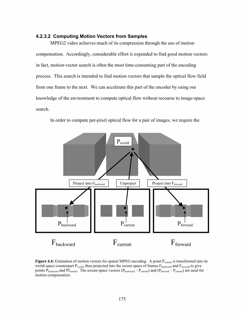
175

4.2.3.2 Computing Motion Vectors from Samples MPEG2 video achieves much of its compression through the use of motion

compensation. Accordingly, considerable effort is expended to find good motion vectors:

in fact, motion-vector search is often the most time-consuming part of the encoding

process. This search is intended to find motion vectors that sample the optical flow field

from one frame to the next. We can accelerate this part of the encoder by using our

knowledge of the environment to compute optical flow without recourse to image-space

search.

In order to compute per-pixel optical flow for a pair of images, we require the

Fcurrent Fforward Fbackward

Pcurrent

Pworld

Unproject Project into Fforward Project into Fbackward

Pforward Pbackward

Figure 4.4: Estimation of motion vectors for spatial MPEG encoding. A point Pcurrent is transformed into its world-space counterpart Pworld, then projected into the screen space of frames Fbackward and Fforward to give points Pbackward and Pforward. The screen-space vectors (Pbackward � Pcurrent) and (Pforward � Pcurrent) are used for motion compensation.

176

camera pose for both images as well as an estimate of the depth at each pixel. This

information is present in the original environment scans. The following algorithm,

illustrated in Figure 4.4, is employed to compute the optical flow from a frame Fcurrent to a

frame Fbackward given the cameras Ccurrent and Cbackward used to acquire each frame.

First, define the following transformation matrices and their inverses for a camera

C:

Windowing transformation (view-frustum coordinates to screen coordinates):

=

100021

2100

20

20

200

2

)(hh

ww

CW

−

−

−

=−

10001200

10210

10021

)(1

h

w

CW

where w and h are the viewport width and height (in pixels).

177

Perspective projection (camera coordinates to view-frustum coordinates):

+−−

−

+−

+−

=−

FNNF

FNNF

NBT

NBT

NLR

NLR

CP

2200

10002

02

02

002

)(1

−−

−−

−

−+

−

−+

−

=

0100

22

00

020

002

)(

NFFN

FNNF

BTBT

BTN

LRLR

LRN

CP

where L, R, N, F, T, and B are respectively the distances to the left, right, near, far,

top, and bottom planes of the view frustum. This matrix is identical to the one

constructed by the OpenGL function glFrustum() [OpenGL ARB 1992, p.

131].

Modelview transformation (world coordinates to camera coordinates):

=−

1000

)(2222

1111

0000

1

czyxczyxczyx

CM

⋅⋅⋅

=

1000

)(210

210

210

czzzzcyyyycxxxx

CM

where vectors x, y, z, and c are the axes and origin of camera C�s coordinate

system. This matrix accomplishes the same purpose as the sequence of operations

178

performed by the OpenGL gluLookAt() function [OpenGL ARB 1992, p. 323,

and Woo et al. 1997, p. 116].

These transformations will be used to find the screen-space location in frame

Fbackward of every pixel in frame Fcurrent. To do that, we need two more transformation

matrices:

( )currentCV 1− , the inverse of the view transform for camera Ccurrent:

( ) ( ) ( ) ( )CWCPCMCV 1111 −−−− =

and V(Cbackward), the view transform for camera Cbackward:

)()()()( CMCPCWCV =

We can now find the screen-space location pbackward in Fbackward of each point

pcurrent in Fcurrent. This is accomplished by inverting the projection matrix used for frame

Fcurrent in order to construct a mapping from screen space to world space. The result of

this inversion is pworld, the world-space counterpart to pcurrent. Finally, pworld is projected

into frame Fbackward to give point pbackward.

currentcurrentworld pCVp )(1−=

worldbackwardbackward pCVp )(=

Finally, the optical flow vector f at point pcurrent is given by the following formula:

( ) currentbackwardcurrent pppf −=

179

This process yields a single motion vector f(p) for each pixel p in the frame being

encoded. Since motion vectors are encoded on a per-macroblock basis, we must examine

up to 256 separate vectors to find the best match. However, this worst-case scenario is

extremely rare in practice. After removing all duplicate motion vectors there are often

only 2 or 3 candidates for each macroblock. The best vector is selected from these

candidates by computing the magnitude (measured as the sum of absolute differences) of

the difference between the macroblock under consideration and the pixels used as its

predictive base. The motion vector that yields the smallest error term is used in the actual

database. Once we have computed a motion vector for each macroblock of Fcurrent with

respect to Fbackward, the entire process is repeated with respect to Fforward to yield a second

motion vector for each macroblock. We evaluate the magnitude of the error term

generated by a motion vector by computing the mean squared error of a predicted

macroblock with respect to the original intensity values. We encode the motion vector

for whichever of Fforward or Fbackward results in the smallest error term. The availability of

motion vectors from two separate source frames increases the probability of finding a

good match for the predictive base since objects occluded in one frame will often be

visible from another nearby viewpoint.

On occasion, we will encounter a macroblock for which no good motion vector

exists. This situation arises when the optical flow in a region is not well approximated by

a translation. The most common examples of this include visibility events causing

geometry to become newly visible or newly occluded. These cases can be detected by

first calculating the magnitude of the error term Eintra using an all-black macroblock as a

predictive base. Any motion vector resulting in an error term greater than Eintra indicates

180

that it is actually cheaper to forego motion compensation entirely and intra-code the

given macroblock.

An example dependency structure for motion compensation between macrocubes

is shown in Figure 4.3. I-cubes are evenly spaced throughout the database. The space

between I-cubes is filled with B-cubes. The frames in a B-cube are predicted from the

corresponding faces from the nearest two I-cubes: as a result, no more than one face of

two different I-cubes must be decoded in order to access any face of any B-cube.

4.2.3.3 Runtime Decoding and Access

At runtime, we decode the frames needed to reconstruct the far field for the user�s

current viewpoint. Whenever the user�s current cell changes, we identify the macrocube

corresponding to the new cell, decode the macrocubes in the predictive base (if the

current cell corresponds to a B-cube), then decode the B-cube itself. Decoded frames are

cached and reused to exploit temporal coherence in the user�s viewpoint. Moreover, intra

cubes are cached separately from B-cubes: since a single I-cube can be used as a

predictive base for many different B-cubes (e.g. all 8 B-cubes out of each group of 9

cubes in Figure 4.3), we can reduce the cost of future database accesses by caching I-

cubes for as long as possible. In order to increase the capacity of such a cache, impostors

are stored in a semi-compressed representation consisting of dequantized DCT

coefficients. We finish the decoding process by applying the inverse DCT and

converting from the native YUV color space to RGB only when frame from the database

is needed for use as a texture map in an impostor. By maintaining a small (1 to 4 cubes)

cache for decompressed impostors and a larger one for the semi-compressed format

181

described above, we are able to fit many more impostors in the space occupied by a

single uncompressed image.

4.2.3.4 Analysis: Advantages of Spatial MPEG By sacrificing strict compatibility with standard MPEG2 video it becomes

possible to encode the 3D structure of the impostor database directly. This eliminates the

discontinuities introduced by laying out the 2D cell grid into a linear stream. As a result,

accesses to cells near the user�s current viewpoint correspond directly to accesses to

nearby frames in the database: when the user enters a new cell, we generally decode at

most the macrocube corresponding to the cell just entered. Since each I-cube is part of

the predictive base for all of its surrounding B-cubes, the cost of decoding and caching I-

cubes is amortized over the time the user spends in any of their corresponding B-cubes.

Moreover, if the walkthrough application imposes reasonable limits on the user�s velocity

and allows speculative prefetching, it is often possible to have a macrocube (intra- or

predicted) already decoded when the user enters a new cell. This allows the system to

avoid distracting pauses while impostors for a new cell are being fetched from disk.

Computation of motion vectors based on the per-pixel information present in the

samples gave good results. By starting with the optical flow field instead of an

uninformed image-space search, the encoder was able to construct a set of good

candidates for each macroblock. Many of these candidate vectors were identical: in the

power plant impostor database containing 3,336 B-cubes (20,016 images), each

macroblock had an average of 4.9 unique motion vectors. As a result, the encoder tests

just a few motion vectors to find the best candidate instead of spending its time on a less

accurate image-space search. However, this introduces the need to load per-pixel depth

182

and per-frame camera information from disk, which is a significant expense. We

compared our model-based motion vector estimation with motion vectors computed with

logarithmic search in a 64-pixel window (a standard encoding technique). Our approach

required slightly longer than logarithmic search (180 minutes vs. 169 minutes on average,

a 6.6% increase in encoding time). However, we observed empirically that for a given

compression ratio, the output of spatial video encoding produces fewer artifacts than

logarithmic search. If we adjust the compression ratio on the log-search encoder to

produce similar image quality, we find that the compressed frames produced by spatial

video encoding are between 8% and 32% smaller than those produced with logarithmic

search. Finally, the selection of macroblocks to be intra-coded in B-cubes was able to

identify and compensate for difficult cases in both the house and power plant models.

Figure 4.5 illustrates a few examples.

183

Figure 4.5: Classification of macroblocks in faces of B-cubes. The left column shows images as stored in the spatial MPEG database. The right column shows the type of each individual macroblock. Regions outlined in red are intra-coded. Regions outlined in green are normal predicted (B) macroblocks. Blue macroblocks are not coded at all: this occurs when the encoder decides that the parameters for the last B-macroblock are adequate for the block being processed. The encoder chooses to intra-code a given macroblock when doing so results in a signal of smaller magnitude than predicting it. This occurs often in regions of uniform color (as in the power plant wall at top), regions of poor prediction due to occlusion (seen in the door grille in the lower right of the music room in the center row), or in regions with particularly fine detail (as seen in the magnified view of the music-room window in the bottom row).

184

4.2.3.5 Analysis: Disadvantages of Spatial MPEG We observed two common artifacts in the images contained in the spatial database.

The first type occurred in cases where our assumptions about the optical flow field were

violated, resulting in motion vectors pointing at a predictive base that did not well

approximate the macroblock being encoded. In such cases we observe �ghosts� visible

on flat, uniformly colored surfaces such as walls. Figure 4.6 shows an example. Ghost

artifacts appear when the geometry visible in the predictive base was occluded by some

flat surface in the current macroblock: as a result, the encoder is forced to fit the negative

of the entire predictive base plus the actual visible surface into the error term, which is

actually meant to only capture small, high-frequency differences between images. These

artifacts could be reduced by identifying poor matches between the predictive base and

the current macroblock and biasing the encoder to intra-code such blocks. The second

Figure 4.6: Ghosting artifacts appear when the MPEG encoder attempts to represent an area of uniform color using motion compensation from a more complex part of a reference frame. From left to right, this figure shows the original, uncompressed image (a), the encoded version present in the MPEG database (b), and the reference image from which it was predicted (c). The silhouettes of the girders in image (c) can clearly be seen on the right of the encoded image (b). Situations such as these could be alleviated by using model information to determine when a particular group of pixels in a frame is or is not a good predictive base for some target region. These images have been contrast-enhanced to highlight the artifacts.

(a) (b) (c)

185

type of artifact, shown in Figure 4.7, appears when the encoder compresses smooth

regions of slow variation. The blockiness visible in the decoded frame is a result of the

8x8 DCT failing to capture the low spatial frequencies contained in the diffuse

illumination. This same blockiness is present in the strict-compatibility implementation

described in Section 4.2.2.

186

Figure 4.7: Blockiness in situations where the 8x8 DCT fails to represent smooth gradients. The image at bottom is from the original sample of the environment. The image at top is the version stored in a spatial MPEG database. This problem can often be alleviated by reducing the quantization factor during encoding.

5 Incremental Spatial Encoding of Textured Depth Meshes

5.1 Introduction

In this chapter we present a method for constructing impostors similar to textured

depth meshes (TDMs) from an incrementally represented set of samples of an

environment. A textured depth mesh consists of a simplified polygonal mesh constructed

from sampled depth values and a high-resolution image that is projected onto the mesh at

runtime. The idea behind textured depth meshes draws upon a technique for building

scenery for a stage production. Rather than construct objects in full geometric detail,

including features that will not be visible from the audience�s fairly distant perspective,

one can create a papier-mâché shell of roughly correct dimensions, then paint it so that

from locations in the audience, the shell looks like the objects being impersonated.

Although this representation is imperfect, it is often good enough to stand in for objects

that are not the focus of attention. Moreover, the shell (impostor) is far less expensive to

construct than exact representations of the scenery in question. The textured depth

meshes we discuss are similar in concept but replace the papier-mâché shell with a

simplified polygonal mesh and the hand-painted surface with a texture map.

The image and geometric parts of a TDM have very different properties. Images

are well-suited to preservation of high-resolution, high-frequency detail and surface

properties because the underlying primitives � individual pixels � depend only on

188

information in a small neighborhood (often the single pixel itself) and cover a very small

portion of the total area. The underlying polygonal mesh is better suited to capturing

regions with sharp boundaries and little internal detail. Since a triangle mesh is defined

topologically in terms of its edges and vertices rather being tied to screen-space locations,

it is possible to capture large areas of little or no variation with a small number of

primitives. Moreover, there are typically restrictions on the possible set of viewpoints

and viewing angles for any given textured depth mesh. Impostor-based walkthrough

systems such as [Aliaga et al. 1999, Decoret et al. 1999] use different sets of textured

depth meshes for different view regions within an environment. This suggests that

simplification of the geometric component of a textured depth mesh can take into account

the visible simplification error with respect to its particular view region instead of relying

on absolute world-space error measures.

The chief drawback of textured depth meshes is their behavior around

disocclusions where geometry should be visible that was not present in the input sample.

Image-based rendering approaches use structures such as the layered depth image (LDI)

[Shade et al. 1998] or multiple-source-image warping [Mark 1999] to fill in this missing

information. This chapter presents algorithms for detecting and removing redundant data

from a set of samples of an environment, then using those same samples to construct far-

field impostors based on textured depth meshes. The resulting impostor representation

achieves some of the same benefits of layered depth images while making use of the

capabilities of graphics hardware.

189

5.1.1 Desired Properties of Geometric Impostors

5.1.1.1 Proper occlusion and parallax In order to provide a reconstruction of maximum fidelity, geometric impostors

should present a faithful impersonation of the far field for as wide a range of viewpoints

as possible. To that end, the incremental TDM representation should exhibit depth

parallax and be capable of self-occlusion. An absence of depth parallax leads to artifacts

such as those visible in Figure 6.1, where straight lines appear to bend when they cross

the border between the near and far fields.

5.1.1.2 Compactness Geometric impostors should occupy as little space as possible in memory and on

disk in order to make them inexpensive to load and cache. Since the impostor database

for complex environments can be far larger than the original primitives, a scalable

Figure 5.1: Perspective artifacts introduced by using impostors texture-mapped onto flat quadrilaterals. The image at left shows the original environment. The image at right replaces distant geometry with an image-based impostor. Straight lines such as the edges of the counters appear to bend where they cross between the near field (represented as geometry) and the far field (represented with an image). Moreover, the proportions and position of the doorway in the center of the image have changed, although this is not as noticeable as the bent lines.

190

walkthrough system must perform some sort of memory management. A compact

impostor representation will allow more room for speculative prefetching and hence

wider flexibility in the areas the user can explore without having to wait for the system to

load missing impostor data.

5.1.1.3 Inexpensive rendering The entire point of using far-field impostors is to provide an approximate

representation for distant primitives that is less expensive to render than the original data.

Moreover, this representation should be compatible with current graphics hardware in

order to free up the CPU for other tasks. In addition to using available resources more

efficiently, a graphics-hardware-friendly impostor representation will allow the

registration of near-field and far-field representations to take place entirely in hardware as

a side effect of rendering. Finally, offloading the impostor rendering process to the

graphics pipeline avoids the (often costly) per-pixel processing associated with purely

image-based methods such as layered depth images [Shade et al. 1998] and light fields

[Levoy and Hanrahan 1996, Gortler et al. 1996].

5.1.1.4 Independence from surface properties Recent advances in real-time computation of complex surface properties such as

programmable shading [Olano and Lastra 1998, Peercy et al. 2000, Lindholm et al. 2001,

Proudfoot et al. 2001], factorized BRDFs [McCool et al. 2001], and surface light fields

[Wood et al. 2000] allow far more flexibility in appearance than the standard per-vertex

lighting and shading model that assumes material properties as part of a polygonal mesh.

Furthermore, complex environments often contain surfaces that are geometrically simple

191

(such as a flat wall in a house) but visually highly complex (as when the wall is covered

with wallpaper). Such high-frequency information should not be included in the

geometric portion of the impostor unless it is actually part of the original surface

geometry. This suggests a strict separation between the image and geometric

components of far-field impostors. Textured depth meshes provide such a separation.

5.1.2 Operations on samples The creation of a compact representation for geometric impostors begins with the

detection and removal of redundant data in the input samples. As in Chapter 4, our input

contains a set of registered samples plus camera information. Unlike Chapter 4, we will

use these samples to create polygonal surfaces. As a result, our comparisons and

modifications will take place between pairs of 3D sample elements instead of between

regions of images (as was the case for spatial video encoding).

5.1.2.1 Comparing Sample Elements The comparison operator for geometric samples is distinct from its image-space

counterpart in two ways. First, it operates on a single point at a time: there is no notion

of similarity between groups of sample elements, nor is there a higher-level structure

such as macroblocks that groups sets of elements. Second, the comparison will return a

binary result rather than a difference measure: instead of computing an error term

between two elements, it will be sufficient to decide whether a given 3D point is

contained within the surfaces captured in a particular sample.

Both of these differences are a result of the support of the process of

reconstruction for polygonal meshes vs. its counterpart for images. In the case of MPEG

or JPEG image compression, discussed in Chapter 2, sections 2.2.1.2 and 2.2.2.3, each

192

image is broken up into 8x8 macroblocks for encoding using the discrete cosine

transform (DCT). As a result, any pixel within a given 64-pixel region can be

reconstructed using only the DCT coefficients for that region. Moreover, the decoded

representation for these images is the same as the input and can be modified on a per-

pixel basis. This is not true for the geometric portion of textured depth meshes.

Although we begin with regularly sampled sets of points, the final result is a simplified

polygonal mesh that can be viewed as a lossy representation of the input points. In such a

situation, each individual point on the mesh has far broader support than the local 8x8

neighborhood of a JPEG macroblock, and as such cannot be modified without also

changing other points. In the case of a highly simplified mesh, such a modification may

affect the entire mesh, not just a spatially small neighborhood!

We will modify the set of 3D points present in a sample of the environment by

detecting and removing points that are present in surfaces captured by other samples.

This process requires the ability to answer the question posed above: is a 3D point P

contained in the surfaces captured by sample R?

5.1.2.2 Altering Range Data Since the comparison operator returns a binary result � whether a particular point

is present in or absent from the surfaces captured by a particular sample � the

modification of samples during the encoding process is limited to complete removal of

any one element. As a result, the problems of global support mentioned above can be

avoided by removing redundant data at the level of individual sample elements, well

before polygonal meshes are created or simplified. This requires that we use the original

193

samples of the environment as input rather than beginning with a set of simplified

textured depth meshes.

5.1.3 Properties of Textured Depth Meshes

5.1.3.1 Advantages A textured depth mesh is composed of a polygonal mesh upon which is projected

an image of the objects represented by the TDM. As such, it is entirely compatible with

current graphics hardware. If the mesh is arranged so that its surfaces pass through the

world-space locations of the points it approximates, the graphics hardware will reproduce

depth parallax and self-occlusion effects as part of the rendering process. Furthermore, it

is straightforward to construct the mesh with regular connectivity that makes it more

amenable to level-of-detail simplification. By changing the parameters of this

simplification, we can allow the user to balance the fidelity of the approximation against

rendering speed. The rendering of TDMs may be further accelerated by keeping track of

the connectivity throughout any simplification and building triangle strips from the final

result. Finally, the geometric portion of a textured depth mesh is completely separate

from the image projected upon it. There is nothing inherent in the impostor

representation that prevents replacing the usual texture map with a more flexible method

such as factorized BRDFs [McCool et al. 2001] or surface light fields [Wood et al. 2001]

that accommodates complex surface properties.

5.1.3.2 Disadvantages In previous work such as [Aliaga et al. 1999, Decoret et al. 1999] a single textured

depth mesh is created from a single sample of some portion of the environment. As a

result, a given TDM only contains information about the points present in each pixel of

194

its original sample. This can result in reconstruction artifacts at viewpoints that should

allow the user to see surfaces occluded in the original sample.

The nature of the errors resulting from incomplete information depends on the

assumptions about the surfaces present in the TDM. The assumption that points

belonging to different objects are actually connected (i.e., the depth buffer is a height

field) will introduce surfaces not present in the original environment (see Figure 1.7 in

section 1.6.2), leading to stretching or rubber-sheet artifacts called skins that were

previously described in Chapters 1 and 3. If instead we include in the TDM only those

surfaces that are positively known to exist in the original environment, gaps called cracks

will appear in areas where occluded geometry should be visible. Since the sample used

to construct a TDM does not include connectivity information, it is not possible to

unambiguously and correctly choose one case or the other. The decision requires

information that is simply not present in a single sample. In Chapter 3, we dealt with the

problem of identifying skins within a set of samples of an environment in order to locate

regions that had not yet been captured. Our approach was to create a coarse current

reconstruction without skins, allowing cracks to form in unsampled regions, and then to

render skins in a later stage to find regions of unsampled space with respect to particular

viewpoints within the environment. The end result of this process was a set of

panoramic samples of the environment. In this chapter, we construct an incremental

representation for those samples that can be quickly rendered as part of an interactive

system. Once again, we want to avoid introducing skins into our representation, this time

to reduce the artifacts present in the reconstruction. The same heuristics used in Chapter

3 to identify edges and surfaces not present in the original environment are employed

195

here to avoid constructing skin triangles. We deal with the cracks left behind when skins

are removed by constructing our impostors to be able to fill in the blanks.

5.1.4 Our Approach: Incremental Textured Depth Meshes We present an incremental representation for textured depth meshes. This

approach creates groups of scan cubes, which are sets of 6 textured depth meshes

arranged in a cube around a central viewpoint. A single scan cube corresponds to a

single panoramic sample of the environment. The two main goals of our approach are to

reduce the redundancy in a set of far-field impostors and to eliminate the cracks and skins

present in regular textured depth meshes. We reduce the amount of redundancy by

establishing a hierarchy over the original panoramic samples and removing from each

sample any surfaces that are visible in any of its ancestors. Second, cracks and skins are

removed from the meshes comprising the faces of individual scan cubes by examining a

set of samples in order to determine whether or not a proposed surface is actually present

in the sampled environment. Only those surfaces that pass this test are included in the

constructed mesh. We further reduce storage and rendering requirements by applying a

view-dependent simplification process to the polygonal meshes created from samples of

the environment. This simplification process takes into account the limited viewing

angles and view volume for far-field impostors. Finally, we describe an algorithm for

identifying the set of scan cubes necessary to construct a view of the far field from any

given viewpoint.

5.1.5 Outline The rest of this chapter is organized as follows. In Section 5.2 we describe the

construction of a set of incremental textured depth meshes without skins from a

196

collection of samples of an environment. In Section 5.3 we present a rendering algorithm

to fill in the cracks in a view of the far field. In Section 5.4 we examine situations in

which incremental TDMs are prone to error as well as situations where they perform well.

Finally, in Section 5.5 we present our conclusions.

5.2 Constructing Meshes from Panoramic Samples

In this section we describe a method for the construction of a set of polygonal

meshes from a set of samples. This process begins with the detection and elimination of

redundant data. Once the size of the input has been reduced, a set of dense, regular

meshes are constructed using the surviving range samples. A view-dependent

simplification algorithm is applied to the resulting dense meshes in order to reduce the

costs of storage and rendering. Finally, we describe an algorithm for selection of a set of

Panoramic sample

database

Build dependency

tree

Identify & remove

redundant points

Per-object

meshes

Simplified ITDMs

Identify skins

Build dense meshes for all surfaces

View-dependent

simplification

Merge surfaces for each sample

Mesh cleanup and triangle strip

creation

Figure 5.2: Construction pipeline for incremental textured depth meshes. Panoramic samples of the environment are divided into connected surfaces. Dense meshes are created without skins for each surface, then subjected to view-dependent simplification. The simplified meshes for each sample are merged into a single mesh, then cleaned up to remove duplicate vertices. The result is a set of textured depth meshes, each of which covers some subset of the surfaces present in one or more panoramic samples.

197

meshes to be rendered in order to reconstruct any particular view of the far field. An

overview of the entire construction pipeline for incremental textured depth meshes is

shown in Figure 5.2.

The simplified meshes in our impostor representation can be viewed as a lossy

representation of the points in the original samples of the environment. The lossiness

occurs in two places. First, strictly speaking, many of the discarded sample elements will

contain information not present in the other samples. This information typically takes the

form of points on a surface that are unique within the environment. This loss does not

necessarily degrade the appearance of the impostors, as discarded points can generally be

recreated by interpolation between nearby retained points. Second, data loss occurs when

a dense polygonal mesh is simplified to reduce the rendering cost of our impostors. It is

not possible to recover the original triangulation or the original point samples from a

simplified mesh. Again, this loss of data is not a significant problem. The simplified

mesh serves as an adequate approximation of the input samples for the particular set of

objects it stands in for. We can compare this simplification to quantization of frequency-

space coefficients in JPEG compression. Although it is not possible to recover the exact

input data from the final, compressed representation, the information lost usually makes

little difference to an observer.

5.2.1 Redundant Sample Detection and Removal The notion of a redundant sample rests on the assumption that one data set

supersedes another: that is, it is adequate to have a particular datum present in one place

instead of two. Standard MPEG2 video compression embodies this notion in its group-

of-pictures structure (see Section 2.2.2.3.1), where every frame in a group of pictures

198

except the first depends on at least one other and encodes only that information not

present in its parent frames. The spatial video database presented in Chapter 4 uses a

similar structure: intra cubes have no ancestors, and predicted cubes contain information

that cannot be predicted from either of the two nearest intra cubes. When constructing

polygonal meshes, samples are first separated into groups. A dependency tree is then

constructed within each group.

5.2.1.1 Groups of Samples The guiding criterion for partitioning the original database of samples into smaller

groups is that each group should contain one scan incorporating the majority of the

information present in all of its counterparts. This suggests that samples taken on either

side of a wall should not belong to the same group, as each contains many samples not

present in the other.

We define a scan group as the set of panoramic samples chosen by the error-

bounded sampling scheme described in Chapter 3. One of the conditions for the creation

of a scan group is that the sample locations are contained within a region of empty space.

Since this region is guaranteed by definition to be free of occluders we expect a large

amount of coherence in the visible geometry for each scan and hence a large number of

redundant samples.

5.2.1.2 Building a Dependency Tree Once scan groups have been established, we construct dependencies within each

group that will guide the detection and removal of redundant samples. We classify the

samples within a scan group into a single intra scan and many delta scans. The intra

scan is analogous to the intra cubes in the spatial video database of Chapter 4 in that its

199

contents are represented without reference to other samples. Delta scans are constructed

with reference either to the intra scan or to another delta scan. Each delta scan contains

only those surfaces not present in any scan on which it depends. This dependency

structure forms a tree over the samples in a scan group.

We identify intra scans and delta scans during the construction of the dependency

tree. A good intra scan maximizes the amount of coherence between its visible surfaces

and the surfaces captured in any delta scan. We guide the choice of the intra scan with

the heuristic assumption that samples taken from nearby viewpoints will tend to have

more in common than those taken from viewpoints farther apart. This suggests that the

intra scan should be chosen to minimize the distance to any other sample in the scan

group. We use the same distance heuristic to construct the rest of the dependencies

within a scan group. In practice, we choose the sample whose viewpoint is closest to the

centroid of all sample locations to be the intra scan.

We build the dependency tree D within a scan group by constructing a complete

graph on all the scans in the group, then assigning a weight to each edge proportional to

the cube of its length. The cubed distance is used as the edge weight in order to avoid

creating trees of depth 1. If we use the linear distance between vertices as edge weights,

then the triangle inequality in the plane ensures that every child node will be connected

directly to the root. A similar situation occurs if the squared distance between nodes is

used as the edge weight. Deeper trees will usually yield better results when removing

redundant samples: since a sample in a given sample is only tested against its ancestors, it

is possible for a single surface to be represented multiple times along parallel branches in

the dependency tree.

200

After constructing a complete graph on the viewpoints for the scan group, the

dependency tree D for that group is defined as the minimum spanning tree whose root is

the (previously specified) intra scan. This tree may be found in O(V + E log E) time

where V and E are the number of vertices and edges in the graph. Since this is a complete

graph, 2VE = , so the overall complexity is dominated by V2. This is not a problem in

practice since V is typically small (at most 30, frequently under 10) and the comparisons

made in the spanning-tree algorithm require no reference to the original environment.

Although the distance heuristic above generally gives good results, it offers no

guarantees on the quality of the spanning tree or the choice of intra scan. It is possible

(though highly inefficient) to find the best possible choice for an intra scan in any group

by constructing a minimum spanning tree for each scan in the group, then performing

redundant sample removal using that tree. The tree with the highest percentage of

redundant samples overall is then the optimal choice. Similarly, it is possible to

determine the absolute best possible spanning tree (not necessarily an MST by the criteria

above) by constructing the set of all spanning trees on the complete graph of samples,

then performing redundant sample removal on each candidate tree to find the best one. In

practice this is prohibitively expensive: finding the optimal root requires performing

redundant sample removal O(V) times (once for each sample), whereas finding the

optimal root and spanning tree requires testing O(VV) trees!

5.2.1.3 Removing redundant sample elements Once a dependency tree has been established for a group of samples we proceed

with the identification and removal of redundant elements. An element s in a sample R is

201

considered redundant if it is already present in any sample along the path from R to the

root of D. This test works as follows:

1. Compute the mapping from R into world space. Use this mapping to

transform the screen-space point s to its world-space location s´

2. Find the distance dexpected between s´ and the sample location for a different

sample R0

3. Project R´ into the screen-space point s0 in sample R0

4. Map the element at location s0 from sample R0 into its world-space location

snew

5. Find the distance dactual between snew and the sample location for R0

6. If dnew and dactual are equal to within some relative error ε, range sample s is

redundant.

Pseudocode for this test is given in Appendix A.

The equality tolerance increases with the distance from the viewpoint to the

sample point to account for the decreasing precision of the depth buffer with increased

depth.

The complete algorithm for redundant sample removal iterates over every depth

sample s in every scan R of the environment and tests it in turn against all of R�s ancestor

scans. The algorithm follows:

R0 = R

while parent(R0) != R0 do

R0 = parent(R0)

if sampleRedundant(s, R, R0) then

DELETE POINT s AND TERMINATE

202

endif

end

Pseudocode is given in Appendix A.

5.2.2 Creating a Dense Mesh Redundant element identification and removal happens at the level of individual

samples. Once this process has terminated, the next step is to create a polygonal mesh for

each face of each sample in preparation for level-of-detail simplification. In order to

avoid unnecessary cracks or skins in the reconstruction (as can happen with some point-

based impostor schemes), the mesh is created as a continuous surface wherever we can be

reasonably sure of surface connectivity. This requires examining other samples in order

to determine the adjacency between each element in each face of each sample and its

eight neighbors in screen space. We use the same heuristics described in Section

3.4.2.1.1 to find this adjacency.

5.2.2.1 Constructing triangles Per-pixel adjacency information is used to construct a polygonal mesh covering

all valid samples in the scan group. This section describes the algorithm to build this

mesh for one face of one sample.

5.2.2.1.1 OpenGL pixel spacing and mesh vertices In order to seamlessly cover the entire space surrounding the viewpoint, a mesh

should subtend exactly the same solid angle as the view frustum of its input range image.

To ensure this, we cover each pixel in the frame buffer with two triangles. The locations

of the vertices of these triangles in screen space [Woo et al. 1997] are shown in Figure

5.4.

203

A B C

D E

F G H

P

Current pixel (to be covered by triangles)

Neighboring

Pixels involved in depth

New vertex

Figure 6.4: Interpolation of neighboring depth samples to create mesh vertices. The adjacency information computed earlier eliminates samples from surfaces that are not connected to the center pixel.

Figure 6.3: OpenGL pixel spacing and sample locations. Position (0, 0) is in the lower left corner of the window. The pixel at (x, y) covers the square between (x, y) and (x+1, y+1). The color and depth value of that pixel is sampled along a ray from the eye through point (x+0.5, y+0.5).

0 1 2 3 4

0

1

2

Screen-space location of color/depth sample Area covered by a pixel

204

5.2.2.1.2 Interpolating between samples Since OpenGL samples the depth for each pixel at the center of the pixel instead

of the corners, we must interpolate between adjacent pixels to make the vertices of their

respective triangles coincide. This interpolation will use the per-pixel adjacency

information computed earlier. We force created vertices to coincide with the screen-

space corners of the pixel by averaging only the depth components of neighboring pixels

and fixing the screen-space position as shown in Figure 5.5.

5.2.2.1.3 Algorithm for covering a pixel with two triangles The following algorithm generates triangles to cover one particular pixel of one

particular range image.

1. For a given pixel p = (x, y, z):

2. Northwest vertex: Find the average depth daverage of p�s neighbors to the north,

northwest, and west. Only include those neighbors that are not connected to p

by a skin edge.

3. Estimate the screen-space location pS = (x-0.5, y+0.5, daverage)

4. Estimate the world-space location vNW by mapping pS into 3 dimensions.

5. Repeat steps 2-4 for the northeast, southeast, and southwest vertices vNW, vSE,

and vSW.

6. Create two triangles with vertices (vNW, vSW, vSE) and (vNW, vSE, vNE).

Pseudocode is given in Appendix A.

205

This algorithm is invoked on every pixel of every face of every sample except for

those samples deemed redundant during earlier processing. The result is a set of dense,

regular meshes, one for each of the six faces of each scan cube. These meshes are too

complex to use directly in TDMs: at two triangles per pixel, a 512x512 range image will

generate up to 524,288 triangles per face or up to 3.1 million triangles for the entire base

scan. Due to their regular structure these meshes are eminently amenable to geometric

simplification.

5.2.3 Mesh simplification Our approach to geometric simplification of impostor meshes is guided by the

role these meshes will play in a walkthrough system and, more particularly, by the way

we reconstruct textured depth meshes. First, since far-field impostors are valid only for a

certain viewing region, it is safe to ignore any errors that will not be visible from within

Existing points

New point

Viewpoint

Ray from viewpoint through screen-space location of new point

Figure 5.5: Interpolation between existing points to create vertices for new triangles. Since triangles completely cover a single pixel in screen space, their vertices must coincide with the screen-space boundaries of pixels as shown in this 2D example. To enforce this, we restrict the new point to a ray through the desired screen-space location and compute its depth along that ray as the average of all contributing points.

206

that region. This suggests a much higher tolerance for errors along the Z axis (parallel to

the user�s view direction) than in the X and Y dimensions (perpendicular to the view

direction): since an error in Z can only be viewed obliquely, a much greater error is

required to produce the same screen-space deviation as a smaller error in X or Y. This is

illustrated in Figure 5.6. Although large errors in depth may be acceptable, there is

almost no tolerance for screen-space deviation of sharp boundaries in the mesh. Since

textures will be applied to TDMs using projective texturing instead of per-vertex texture

coordinates, the texture will not deform with the geometry. Instead, simplification errors

perpendicular to the view direction will cause the projected texture to appear partly on

vx

s

p∆x∆x

e

f

z

∆z

∆x

screen

p´

Figure 5.6: Relative world-space error for a given screen-space error. Given a viewpoint v at the origin, a world-space point p=(x, z) is projected to the screen-space location p´. In order to produce an error of magnitude e toward the screen-space center of projection, p may be moved toward the camera by ∆x units (along the x-axis) or away from the camera ∆z units (along the z-axis). As the error e approaches the distance fbetween p´ and the center of projection, the error ∆x is bounded above by x while the error ∆z can grow without bound.

207

surfaces neighboring the locus of error. This produces distracting �ghost� outlines (see

Figure 5.7) in the reconstruction. The outer boundaries of a mesh must be treated with

similar care: in order to assemble sets of six TDMs seamlessly into cube environment

maps, their edges must meet cleanly with no gaps. These different levels of error

tolerance suggest a view-dependent simplification scheme such as those described in

[Luebke and Erikson 1997, Hoppe 1997, Xia and Varshney 1996].

Tolerable levels of simplification error are selected based on proximity to sharp

boundaries in the mesh. Points along the outer borders of a mesh or along silhouette

edges visible from the viewing region are not allowed to deviate from their original

locations by more than half a pixel. Points in the interior of a mesh have considerably

more latitude for error. Given an error tolerance, simplification proceeds in two steps.

Figure 5.7: Single-pixel errors in the registration between the image and geometric portions of incremental textured depth meshes can cause distracting �ghost� outlines as seen on the wall to the left of the archway. These outlines properly belong to other surfaces in the model. Ghost outlines of the archway are also faintly visible along its right side at the far rightof the image.

208

First, a view-independent algorithm (GAPS, described in [Erikson and Manocha 1999])

is employed to generate a sequence of vertex merges for the original mesh. Second,

view-dependent criteria are employed to choose a subset of those vertex merges to create

the final TDM. In this section we describe the details of these two phases.

5.2.3.1 Stage 1: Generating a vertex merge tree We begin simplification by constructing a view-independent sequence of vertex

merges using a modified version of the simplification scheme described in [Erikson and

Manocha 1999], which in turn is based on [Garland and Heckbert 1997]. Both of these

methods perform simplification by collapsing an edge into a single vertex and removing

the triangles bordered by that edge. Moreover, both methods use the notion of quadric

error metrics to keep track of the cumulative simplification error as more and more edges

are eliminated. Although this approach can produce high-quality drastic simplifications,

it often creates fans of very long, thin sliver triangles in regularly tessellated planar

regions (see Figure 5.12). Such regions are quite common in our application. The

incidence of sliver triangles can be reduced by modifying the sorting criterion between

candidate edge collapses (see [Jeschke and Wimmer 2002]), but it is difficult to eliminate

them entirely and still maintain single-pixel accuracy at the edges of a triangle mesh.

The output of the view-independent simplification is a sequence of vertex merges

that form a tree. The leaf nodes of this tree are the original vertices of the mesh. The

interior nodes are vertices created by vertex merges or edge collapses. The root of the tree

is the single vertex left when all edges in the mesh have been collapsed. Each edge in the

tree represents the collapse of a single edge in the mesh. Interior nodes are annotated

209

with the error introduced by their corresponding edge collapses as well as the resulting

changes in mesh connectivity. A cut of this tree constructed according to the view-

dependent criteria described below produces the actual simplified mesh.

5.2.3.2 Stage 2: View-dependent simplification The goal of view-dependent simplification is to choose a set of edge collapses in

the view-independent tree that results in a mesh with as few triangles as possible while

still satisfying screen-space error bounds. These bounds are tightest around silhouette

edges and mesh boundaries in order to avoid introducing cracks in the reconstruction.

Since the input mesh was created with known connectivity, we can identify the edges

with low error tolerance. A boundary edge is one that is adjacent to exactly one triangle.

A silhouette edge with respect to a view direction is defined as an edge shared by two

adjacent faces, one facing toward the viewer and one facing away. Since we know the

extent of the view region for the meshes we are simplifying, it is possible to identify all

potential silhouette edges by taking four viewpoints (one at each corner of the view

region) and constructing the union of the set of silhouettes with respect to each viewpoint.

Once we have identified the silhouette and boundary edges for a particular mesh,

we choose a view-dependent simplification by identifying a set of edge collapses that

does not introduce any visible screen-space error along the boundaries and silhouettes.

This tolerable set contains a complete list of the vertices in the simplified mesh: in turn,

the nodes corresponding to these vertices form a cut of the vertex merge tree constructed

in the previous section. The vertex set is populated by repeatedly examining each node in

the current cut to see whether its corresponding edge collapse would exceed the error

budget for that edge�s neighborhood. If so, the node is left unchanged; if not, the node is

210

replaced by its parent and the appropriate changes are made to the mesh structure. The

algorithm terminates when none of the nodes in the cut can be safely collapsed. The

initial cut of the tree consists of all the leaf nodes. This algorithm is presented below

with pseudocode in Appendix A.

1. Initialize the current cut to contain all the leaf nodes of the vertex merge tree

2. Until convergence, iterate steps 3-4:

3. For each node n in the cut:

4. If collapsing n introduces a tolerable screen-space error, then perform the edge

collapse, modify the mesh accordingly, and replace n with its parent in the

current cut.

5. Terminate when the entire cut has been traversed without collapsing any

edges.

5.3 Rendering the far field using a tree of scan cubes

Once the processes above are completed, the following data are available:

• A set of simplified polygonal meshes (six meshes, one for each face of a scan

cube corresponding to one of the original samples of the environment)

• The viewpoints of the cameras used to acquire the original samples

• A tree whose nodes are those viewpoints and whose edges describe the

dependencies between scan cubes (for purposes of redundant sample removal)

We also assume access to the images that will be used to texture these meshes. In

order to present the user with a reconstruction of the objects represented by these

impostors, we must identify a set of scan cubes that are likely to collectively contain all

211

objects visible from the user�s current view. This identification can also incorporate a

user-specified triangle budget to balance fidelity against rendering speed.

The identification of a set of scan cubes to render begins with the assumption that

nearby viewpoints lead to similar views of an environment. As a result, we choose the

scan cube whose sample location is closest to the user�s viewpoint as the best

approximation of the far field. Since a scan cube S constructed from a delta scan only

contains portions of surfaces not visible in any of its ancestors, we also include the

ancestors of S up to and including the intra scan. The expense of rendering all of the

ancestor scans is generally only slightly higher than that of rendering the intra scan alone

since the majority of the points in a sample (on average 98% in the house and 89% in the

power plant) are removed as redundant during mesh creation.

After the initial set of scan cubes has been identified, view-frustum culling

eliminates meshes within each cube that are definitely not visible. At this point more

scan cubes can be selected for rendering. If the user is attempting to maintain a constant

frame rate, new cubes can be added until the total set of geometry to be rendered meets a

user-specified triangle budget. If the user prefers to maintain image fidelity at the

possible cost of lower frame rates, new scan cubes will be added until a certain number of

scans have been identified for rendering. In either event, new scan cubes are added by

identifying the closest cube Snew to the user�s viewpoint that is not yet in the renderable

set. As before, the ancestor scans of Snew are also marked for rendering. Again, this is a

relatively inexpensive operation: due to the construction of the dependency tree, nodes

with nearby viewpoints tend to have many common ancestors. In the power plant, for

example, the average intra cube contains 221,542 polygons whereas the average delta

212

cube contains 70,340 polygons, only 31% of the size of an intra cube. The statistics for

the house � 8,334 polygons per intra cube and 5,605 polygons per delta cube on average

� are not representative due to the low visual complexity of the environment.

Nonetheless, we note that 5,600 polygons is a low additional cost when the per-frame

polygon budget can be up to 250,000 triangles.

We note that the savings in the polygon counts for delta cubes are less than the

fraction of the points that were removed as redundant. When our algorithm identifies and

removes sets of points from the samples that will become delta cubes, it creates new

screen-space boundaries that are preserved exactly by the view-dependent simplification

algorithm. These boundaries are not present in the intra cube, allowing a far more drastic

simplification for the same visual fidelity. Nonetheless, the benefits of removing

redundant samples are considerable, since the surfaces in delta cubes tend to be clustered

into small groups that are easily culled. In practice, we rarely render more than half of

the polygons in a delta cube for any viewpoint.

In the event that Snew and its ancestors exceed either the per-frame triangle budget

or a scan budget, we remove scan cubes starting at Snew and working upward toward the

root until the budget is met. Since the set of renderable cubes fell within the per-frame

budget before Snew was selected, this process of removal will not eliminate any scan

cubes on which others depend.

We continue to identify nearby scan cubes and add their ancestors to the

renderable set until either enough have been selected or the per-frame triangle budget has

been exhausted. The scan cubes in the final renderable set are drawn into the frame

buffer to provide the user with an approximate reconstruction of the far field.

213

5.4 Analysis

We have applied the methods described in this chapter to create sets of textured

depth meshes for two different architectural environments. The first was a model of a

house containing approximately 261,000 polygons and 19 megabytes of high-resolution

textures. The second environment was a model of a coal-fired power plant containing

some 12.7 million polygons. In each case, we selected interesting subsets of the model as

our test cases. This section discusses our observations of the performance of incremental

textured depth meshes in these environments. Full details of the implementation will be

presented in Chapter 7.

5.4.1 Computational Complexity In this section we describe the computational complexity of the process of creating

incremental textured depth meshes. We consider the cost of each step of the algorithm as

well as its overall behavior. Statistics for the performance of our methods on real-world

data sets are presented in Chapter 7.

5.4.1.1 Building the dependency tree The dependency tree that guides the removal of redundant points from a group of

samples is created from a complete graph constructed on the sample locations. This

graph has O(n) vertices and O(n2) edges with respect to the number of samples. The

minimum spanning tree for a graph with V vertices and E edges can be computed in O(E

log V) time using ordinary binary heaps or O(E + V log V) time using Fibonacci heaps

[Corman et al. 1990]. As a result, the asymptotic complexity of creating the dependency

tree is O(n2) in the number of samples. In spite of this result, this operation is the fastest

part of the overall process: it requires only the 3D location of the viewpoint of each

214

sample and typically operates on 10-15 samples. Moreover, the dependency tree is only

created once for each group of samples and requires no per-pixel processing.

5.4.1.2 Removing redundant points The heuristics for identifying and removing redundant points are evaluated once

for each pixel of each face of each sample. Since each point can be compared against

surfaces in every other sample (at worst), the per-pixel complexity is O(n) in the number

of samples. Performing this operation on O(n) samples leads to a worst-case complexity

of O(n2). In practice, this process usually exits after 1 or 2 comparisons instead of

checking all O(n) samples.

5.4.1.3 Identifying skins We use the heuristics described in Section 3.4.2.1.1 to identify skin edges within

each sample. As described in Sections 3.5.1.1.1 and 3.5.1.2.2, these heuristics have a

per-pixel complexity of O(n) in the number of samples, leading to an overall complexity

of O(n2) for a group of n samples.

5.4.1.4 Mesh simplification We use GAPS [Erikson 1999] to perform view-independent simplification and the

method described by Luebke and Erikson [1997] for view-dependent simplification of

dense polygonal meshes. Carl Erikson gives an upper bound of O(n log n) for the

computational cost of using GAPS to simplify a mesh with O(n) primitives.

The view-dependent simplification stage traverses a vertex merge tree containing

one node for each original vertex and one node for each edge collapse. Since an edge

collapse operation removes one vertex from the model, there can be at most n edge

collapses in a model with n vertices and thus at most 2n nodes in the merge tree. We

215

traverse this tree once for each corner of the view region, and at each traversal we may

visit each node in the tree at most once. We traverse a tree with O(n) nodes O(1) times,

leading to a total complexity of O(n) in the number of vertices in the reconstruction for

view-dependent simplification.

The cost of simplifying ITDMs is dominated by the O(n log n) complexity of

view-dependent simplification. In this case, n is the number of triangles in the set of

dense polygonal meshes described in Section 5.2.2. This can be up to two triangles for

each pixel in each sample, leading to up to O(n) triangles in the number of samples. The

overall cost of mesh simplification is therefore O(n log n).

5.4.1.5 Overall behavior The asymptotic complexity of creating a set of incremental textured depth meshes

from a group of n samples is dominated by the O(n2) costs of removing redundant points

and identifying skins. In practice, however, mesh simplification is the most expensive

phase. In Section 7.5.2 we present preprocessing statistics for ITDM creation for several

groups of samples in two different real-world data sets. In both cases, the O(n log n)

mesh simplification phase takes roughly 5 times longer than the O(n2) mesh creation

phase that includes both redundant point removal and skin identification.

5.4.2 Benefits of incremental textured depth meshes

5.4.2.1 Faithful reproduction of environments Our experience has been that incremental TDMs are a good approximation for the

far field in certain kinds of environments. These environments typically have many

smooth, flat surfaces that can be well approximated by just a few polygons. Such

surfaces are well suited to the incremental process of mesh creation and simplification.

216

Moreover, visibility typically changes smoothly in such environments: the closer two

viewpoints are to one another, the more coherence we expect between their respective

sets of visible primitives. This will tend to give good results with tree-based redundant

sample removal: since a given sample�s immediate ancestor is usually close by as

compared to the sampled geometry, a large fraction of its samples will be removed. In

practice, such friendly environments are quite common in architectural models.

5.4.2.2 Removal of redundant information The identification and removal of redundant range samples considerably reduced

the expense of rendering multiple TDMs. The heuristics in Section 5.2.1.3 were able to

detect redundant samples on both flat and curved surfaces. Although there were

problems with accidental removal of samples from surfaces nearly parallel to the view

direction, such cases proved relatively rare. In the living room of the house model, the

redundant-sample detection algorithm removed an average of 94.1% of the points from

each of 27 different delta cubes acquired from a 6-by-4-meter region. In a difficult

region of the power plant model near the furnace, the redundant-sample detection

algorithm removed an average of 89.6% of the samples in each of 62 different delta cubes

taken within a 4-by-2-meter region. Detailed results are presented in Chapter 7.

5.4.2.3 Approximate occlusion culling The nature of textured depth meshes dictates that they only contain information

about the first visible surface. As a result, replacing the far field with a TDM (or set of

TDMs) accomplishes much the same goal as occlusion culling: objects within the user�s

view frustum but occluded by nearby surfaces are not rendered at all. Moreover,

rendering a set of incremental TDMs is similar in concept to culling using region-based

217

(instead of point-based) occlusion. By incorporating information from several

viewpoints instead of just one, the reconstruction of the far field remains valid over a

much larger region than with traditional, single-source TDMs. We note in passing that

we are not attempting to provide an exact visibility solution in our reconstruction: exact

region-based visibility is still an open area of research. Current methods such as

[Nirenstein et al. 2002] show promise for complex environments but at a very high

preprocessing cost. Even if exact region-based visibility were inexpensive to compute, a

less precise approximation might be adequate due to the information lost by sampling the

scene during rasterization.

5.4.3 Difficult situations for incremental TDMs Incremental textured depth meshes perform best in situations with relatively

simple occlusion. Although such situations are reasonably common in the environments

we wish to render, there are plenty of exceptions. In this section we characterize some of

the more common instances that pose problems in the construction of incremental TDMs.

5.4.3.1 Rapidly changing visibility between viewpoints The success of the process of redundant sample depends by definition on

coherence in the visible set between two different viewpoints. This process will naturally

perform poorly in situations where this coherence does not exist. One example of such a

situation is when large occluders are interposed between the viewpoint of a child scan

and its ancestor scan. Fortunately, such situations are rare due to the requirement that the

the region containing the viewpoints for the original panoramic samples of the

environment be free from geometry. If such geometry exists, it is removed during

impostor generation and handled separately (as the near field) at runtime.

218

A less tractable example of difficult visibility occurs when the far field is visible

only through small openings between closely spaced occluders. This situation arises

often in the interior of the power plant, which is full of vertical arrays of thin cylindrical

piping. In such environments, even small changes in viewpoint can produce a large

difference in the set of visible primitives. An illustration of the problem using an example

from the power plant environment is presented in Figure 5.8. Fortunately, the arrays of

pipes are not always so difficult: in fact, for viewpoints at least a few meters away, an

array of pipes can often be reasonably approximated using a single connected, nearly flat

surface.

Figure 5.8: A small change in viewpoint can cause a large change in the set of visible surfaces due to the many thin apertures between objects. This reduces the fraction of sample elements that will be removed as redundant during the construction of incremental textured depth meshes.

219

5.4.3.2 High-frequency components and silhouettes in the depth buffer In order to make the borders of one incremental TDM line up neatly with another,

the simplification process is required to preserve mesh boundaries and silhouette edges in

the original, dense meshes. This can cause problems in configurations with complex

silhouettes, as in Figure 5.9. The simplification algorithm successfully preserves the

high-frequency detail; however, it does so at the cost of many more polygons than we

would like to spend � and more than were in the original objects being represented! We

could simply fill in such holes, but doing so would change the topology of the textured

depth mesh and make it unsuitable for simple projective texture mapping. For example,

if we were to fill in the shadow on the floor (a relatively simple surface) cast by the couch

shown in Figure 5.9, projective texture mapping would place a copy of the image of the

Figure 5.9: Requiring sub-pixel precision when simplifying silhouette edges can lead to poor triangulations. In particular, the silhouette of the couch on the floor has many fans of long, thin triangles along its border. Not all silhouettes are so problematic. The edge of the couch at bottom left, while not as clean as some surfaces, has a much simpler triangulation than the shadow on the floor at right.

220

couch in the foreground on the floor in the background.

Surfaces that produce high-frequency components in a sample are also difficult to

reconstruct even when no silhouettes come into play. This is a signal-processing problem

as opposed to a strictly geometric one: a sample can be viewed as a set of point samples

of the plenoptic function, whereas the reconstructed mesh is an approximation to that

function for a single viewpoint. Since the plenoptic function is not band-limited, it is

entirely possible for closely spaced primitives to result in aliasing in the sampled samples.

In such situations a correct reconstruction of visible surfaces is not possible. This is

sometimes not a problem: for geometry such as the wall of closely spaced pipes shown in

Figure 5.10, aliasing results in a nearly flat surface in the reconstruction. This turns out

Figure 5.10: The wall of pipes shown here can be reasonably approximated as a flat surface. In such situations the finite sampling resolution can produce a much simpler reconstruction than an exact representation of the environment with little or no loss in image quality.

221

to be a reasonable approximation for the densely spaced pipes. We note that similar

configurations are problematic even for unaccelerated rendering using original primitives.

Figure 5.11 shows moiré artifacts that result from scan conversion of high-frequency

portions of the environment.

5.4.3.3 Edges of curved surfaces The algorithm for constructing vertices to cover a single pixel in a sample works

reasonably well for flat surfaces. However, the boundaries of curved surfaces can prove

difficult to handle, since the information necessary to reconstruct the surface�s true

orientation is partially contained in pixels not visible from within a sample. This can

Figure 5.11: High-frequency elements in the environment such as the closely spaced pipes shown here can cause aliasing artifacts even when rendering the original primitives.

222

result in seams (see Figure 5.12) where a single curved object is spread across multiple

samples.

5.5 Summary and Conclusion

In this section we have presented a method for the construction and rendering of

incremental textured depth meshes starting from a database of registered samples of an

environment. By identifying and removing redundant samples within groups of samples,

we are able to reduce the cost of rendering in order to render multiple sets of TDMs at a

time. This combination allows us to present the user with a reconstruction of the far field

that remains valid for a wider region than previous methods. We have further reduced

the cost of rendering through the use of a static, view-dependent method of geometric

Figure 5.12: Seams in incremental TDMs due to curved surfaces being split across multiple samples. The two large pipes just left of the center of the image are partially or wholly occluded by the large pipe at right for much of a view region. As a result, different samples often see different parts of the curved surface, requiring that many meshes be rendered in order to reconstruct the entire object. The seams shown here occur when the edges of the meshes do not line up precisely. This picture was taken outside of the viewing region for the samples shown in order to highlight the reconstruction artifacts.

223

simplification. Overall, we believe that an incremental impostor representation based on

cubes of textured depth meshes provides an efficient, high-quality reconstruction of the

far field for interactive walkthrough of complex virtual environments.

224

6 Common elements of our spatial representations of image-based impostor data

6.1 Introduction

The major new results of this dissertation include image-based and geometric

representations (impostors) for far-field data to accelerate interactive walkthrough. In

both Chapters 4 and 5 we begin with several samples of the environment. Each sample

consists of a cube environment map with color and range data at each pixel plus camera

information for each face of the environment map. However, the representations derived

from these samples are radically different. The spatial video encoding schemes described

in chapter 4 transform our panoramic range samples into a database of flat images

represented using methods similar to MPEG-2 video compression. The methods for

constructing incremental textured depth meshes described in Chapter 5 produce a forest

where each node of each tree contains a polygonal mesh representing some part of the

environment.

In spite of the radical differences in both the form and purpose of the different

impostor representations, we observe that their underlying approaches share a few

common elements. These elements include assumptions about the nature of the sampling

process, abstract operations performed on the panoramic range data, and the notion of

removing redundant information across different samples. The intent of this structure is

226

to detect and reduce the amount of redundancy in a set of samples in order to achieve a

more compact representation than if each sample were processed in isolation. In this

chapter we highlight an underlying structure for our spatial encodings of image-based

simplifications of the far field.

6.1.1 Chapter outline The remainder of this chapter is organized in the following manner. Section 6.2

enumerates the common elements of the construction of spatial representations of far-

field data, including data organization and necessary operators. Section 6.3 describes the

aspects of spatial representations resulting from these common elements. Section 6.4

discusses circumstances under which such a structure may be expected to work well as

well as more difficult scenarios where it may perform poorly.

6.2 Assumptions and operations concerning sampled range data

This section discusses the organization and operations involved in constructing

spatial representations from sampled range data. These elements will allow parts of

samples to be compared: if two parts of different samples are sufficiently similar, it may

be possible to store one at full detail and the other as a (small) difference from the first, or

even to omit one of the two parts entirely and replace it with a reference to the other.

Such comparisons enable compact representations by reducing the redundancy in a group

of samples. The common structure consists of a hierarchical organization for some group

of samples (e.g. all samples whose viewpoints fall into the same room) and a group of

operations to be performed on parts of those samples. Particular aspects of the hierarchy

and the operations will depend on the nature of the intended representation.

227

6.2.1 Assumptions about the input

6.2.1.1 A set of registered range scans In order to identify and remove redundant information across different samples,

we must be able to compare parts of one sample with parts of another. In order to make

this comparison, a common frame of reference must be established by registering each

sample with its counterparts. This dissertation is concerned with range data acquired

from synthetic environments. Since complete camera parameters are available as an

intrinsic part of the sampling process, the registration problem is trivial in such situations.

Range data acquired from real-world environments may be registered using standard

techniques such as iterated closest point matching [Besl and McKay 1992]. The

interested reader is referred to the literature for further details.

6.2.1.2 Static environment with completely sampled surfaces Our impostor representations do not address the problems of texture and surface

extrapolation. Both of these problems deal with the issue of extrapolating missing data

(surface position or texture) from the properties of a surrounding region. See [Williams

and Chen 1993] for an example of texture extrapolation and [Curless and Levoy 1996]

for one approach to surface hole-filling. Since we do not address these issues, any

surfaces that are to be present in the reconstructed environment must be imaged in at least

one sample of the environment. Moreover, range scans are assumed to sample only static

primitives: if the environment contains moving objects, they must be handled separately.

6.2.2 Operations on range data Placing a set of samples into a common coordinate system enables operations that

compare and modify elements belonging to different samples. These operations are

228

intended to detect redundant information within a group of samples and remove it in

order to produce a more compact representation.

6.2.2.1 Integrate new samples into an existing database It is often desirable to construct a spatial representation of an environment using a

sparse initial set of samples. Once complete, this initial representation can be

incrementally updated using data acquired later from regions where a more faithful

reconstruction is desired. Such incremental construction and update requires the ability

to register new samples against an existing database.

6.2.2.2 Compare regions of two range scans In order to determine whether a given set of sample elements is redundant, it must

be possible to compare them with some set of elements from some other sample to

quantify the degree of similarity. This comparison can take place in the image domain

via standard techniques such as mean squared error, the sum of absolute differences,

frequency-domain comparison, or perceptually-based comparison as described in [Daly

1993]. Geometric comparisons (when the input contains points in space) may be

computed using the Hausdorff distance for sets of points, or perhaps with a minimization

approach to estimate a transformation between one set of points and another (similar to

some registration schemes). In any case, the nature of the comparison is specific to the

desired properties of the representation. In Chapter 4 we used an image-space difference

to remove redundant information from a database of compressed images. In Chapter 5

we used a point-on-surface test to identify redundant geometric information, namely

points in one sample that belonged to surfaces already represented in another.

229

6.2.2.3 Remove or reallocate sample elements The comparisons described in the previous section will identify sets of elements

that are present in two or more samples. In order to construct a compact spatial

representation, it must be possible to remove such redundant elements from a sample

while leaving the rest of the data intact. It may also be useful to be able to reallocate such

elements into the sample where their non-redundant counterparts were found in order to

create a denser representation than would be available within a single sample.

6.2.3 Hierarchies of samples The notion of redundant data implies the existence of some sort of hierarchy by

which data in one sample may be considered to supersede another. This hierarchy must

be established on every sample that will have redundant information removed.

As examples, we present two of the hierarchies used in this dissertation. The first

is the group-of-pictures structure (described in Section 2.2.2.3 and addressed further in

Chapter 4) used in MPEG2 video. This structure is equivalent to a directed acyclic graph

with a node for each picture in the group and a single root (the I-frame). A P-frame,

which is stored as a difference from a single other frame, is represented in the graph as a

child node of the frame on which it depends. B-frames are predicted from the contents of

two different frames and are thus represented as nodes in the graph with two parents.

This graph guides the encoding of a group of pictures as MPEG2 video by storing each

frame as a difference from its parent frames (if any). The intra frame at the root of the

graph has no ancestors and is thus stored intact. P- and B-frames contain only data not

present in their immediate ancestors.

The second type of hierarchy we will describe is the dependency tree for a group of

scan cubes or incremental textured depth meshes, presented in Chapter 5. Briefly, this is

230

a spanning tree constructed over the sample locations for a group of samples. As with

MPEG2 video, this tree guides the detection and removal of redundant data. Unlike

MPEG2, however, the sample at any node in the tree will encode only information not

present in any of its ancestors, up to and including the sample at the root of the tree.

Both of these hierarchies can be described as directed acyclic graphs with a single

root. This is not the only permissible structure: although a single root will prove useful

as a predictive base, it is certainly possible to construct hierarchies with multiple root

nodes or even multiple disjoint graphs.

6.3 Characteristics of spatial representations sharing this structure

The elements described in the previous section allow the construction of a compact,

incremental representation of an environment. This representation will be used for

rendering acceleration at runtime by providing an inexpensive, faithful approximation of

the original primitives. By building spatial representations that incorporate the structure

in this chapter, benefits can be realized that are not available when the samples of the

environment are considered on their own. This section discusses those benefits.

6.3.1 Reduced redundancy with respect to the original samples Impostor-based walkthrough systems such as [Aliaga 1999], [Aliaga et al. 1999],

[Decoret et al. 1999], and [Wilson et al. 2001] exhibit considerable redundancy in the

objects visible in their far-field impostors. By identifying and removing redundant data

during the construction process, a more compact set of impostors may be created that

contains all the same visible surfaces. In many of the locations we have examined in the

house and power plant environments, the fraction of redundant samples from one

viewpoint to the next exceeds 90%. This opens up the possibility of incremental

231

rendering of the far field: as time and resources permit, impostors constructed from

nearby viewpoints can be rendered to fill in gaps in the present set. A similar approach to

dynamic updates of the far field is discussed in [Decoret et al. 1999]. Alternately, a

spatial representation may be created that explicitly encodes the data dependencies

necessary to reconstruct a complete view of the environment for each desired viewpoint.

6.3.2 Increased sampling density resulting from reallocated samples Even redundant data can often be used to contribute to the fidelity of the

reconstruction. In general, two finite-resolution sensors observing the same region of a

surface will sample different points within that region. By combining elements from

different range scans, a more accurate, more densely sampled representation becomes

available as an input to the spatial representation. This does not necessarily increase the

size of the finished representation: if some sort of lossy compression method is employed,

the denser sampling may be reduced to a certain size target just as easily as a sparse one.

6.3.3 Access to joint information A set of registered samples contains information that is not present in any single

sample alone. For example, consider the process of building triangle meshes over the

points in a single range scan by treating the individual samples as the vertices of the mesh.

If no information is available apart from the range scan itself along with its camera

parameters, it is not possible to decide with certainty whether an edge between two

samples is actually present in the surfaces being imaged. This information can be made

available by examining other range scans that observe the portion of the surface being

reconstructed. This problem is discussed in detail in Section 5.2.2.1.

232

6.4 Analysis

The structure described in this chapter has been derived from two different far-field

representations using sampled range data. The input samples are typically acquired at

evenly spaced viewpoints from within the environment to be reconstructed. Sample

locations may also be constructed using an incremental approach as described in Chapter

3. Although an even spacing is not essential to the usefulness of the structure, it does

suggest certain properties that affect the efficiency of the treatment of redundant data.

This section concerns characteristics of the input data that are likely to affect the

usefulness of the framework.

6.4.1 Favorable Circumstances

6.4.1.1 Good registration available Comparisons between elements of the same portion of the same surface in

separate samples are only meaningful if the elements under consideration do in fact

represent the same surface. This requires that the samples be well registered with one

another, preferably with a maximum error less than the error inherent in the sensor. In

synthetic environments this is not a problem: range data are acquired at the precision of

the depth buffer (often 32 bits) and precise camera information is available as an integral

part of the capture process. Data acquired from real-world settings may be more difficult

to register precisely: in such situations, the comparison operators will need to account for

the error inherent in the sampling process. Applications to real-world settings are beyond

the scope of this dissertation.

6.4.1.2 Redundant information exists The hierarchical organization of samples and the operations for comparison and

removal of redundant elements operate in situations where two or more samples image

233

the same set of surfaces. As a result, the representations incorporating this structure will

be most compact where there exists a large degree of overlap across the input samples.

Environments with relatively simple visibility (including many architectural and urban

environments) will often exhibit such overlap in samples whose viewpoints are not too

distant from one another.

6.4.2 Adverse Circumstances

6.4.2.1 Little redundancy in samples Redundant sample elements can only be detected, reallocated, or removed when

they exist. As a result, spatial representations built from samples whose sets of visible

surfaces have little in common will realize little benefit from the operations described in

this chapter. This can occur when sample locations are placed in mutually occluded

regions such as on either side of a closed door or in environments with complex, near-

degenerate visibility such as shown in Figure 6.1.

234

6.4.2.2 Poor registration The ability to compare elements from different samples relies on the ability to

correctly identify which regions of one sample correspond to a given region of another.

This in turn relies on an accurate registration of the various samples in order to compute

the transformation from one to another. Without this accuracy many elements that should

properly be identified as redundant will be classified as previously unseen, thus inflating

the size of the resulting representations. This situation can also arise when the

comparison operation is too demanding and requires precision exceeding what the

representation can supply. When samples are acquired with a per-face resolution of

1024x1024 (twice what we use for impostor generation) and a 90-degree field of view,

each pixel will cover a 20cm x 20cm square on surfaces 100 meters from the viewpoint.

Moreover, different samples will rasterize the surface using different points for each pixel.

It is not realistic to expect to be able to make comparisons to within a few millimeters at

such distances when points must be interpolated among such widely spaced samples. A

Figure 6.1: A difficult environment for detection and removal of redundant samples. The sets of points visible from each viewpoint (black circles) have very little in common. Moreover, the regions of overlap (in the horizontal corridor in the center) are subject to high discretization error due to high angles of incidence between surfaces and view rays. This reduces the reliability of surface comparisons.

235

100-meter-deep visual field is quite common in the power plant environment, especially

when the view frustum includes objects outside the building proper.

6.5 Conclusion

In this section we have outlined a common structure present in the construction of

two different spatial representations of environments using sampled range data. This

structure dictates an organization of samples (in our case, range scans) into a hierarchy as

well as the establishment of operations to compare and modify groups of samples (or

even individual samples) within each scan. Although the nature of these elements will

remain constant across different representations, the details of the implementation will

vary according to the needs and goals of the application.

236

7 Implementation and Results

7.1 Introduction

We have implemented the methods described in chapters 3, 4, and 5 for acceleration of

interactive walkthroughs of large geometric environments. In this chapter we describe

the design of two cell-based walkthrough systems that incorporate our approach and

present results obtained from two different data sets.

7.1.1 Chapter Structure This chapter is organized as follows:

In Section 7.2 we describe MPEGWALK, a walkthrough system incorporating

far-field impostors that maintain strict compatibility with standard MPEG-2 video

compression as described in Section 4.2.2.

In Section 7.3 we describe VWALK, a walkthrough system incorporating

spatially encoded video (described in Section 4.2.3) and standard textured depth meshes.

In Section 7.4 we describe the implementation of the Voronoi-based sampling

scheme presented in Chapter 3. We present statistics concerning its performance in the

house and power plant models and show empirical results that support the claim that our

incremental sampling method finds reasonable approximations to the best next view. The

databases of samples created by Voronoi-based sampling will be used to create the

incremental textured depth meshes described in Section 7.5.

238

In Section 7.5 we discuss extensions of the VWALK system to support

incremental textured depth meshes. We compare the performance of incremental

textured depth meshes, which are created from samples chosen with the Voronoi-based

sampling algorithm from Chapter 3, with standard textured depth meshes, which are

created using a single sample for each view region. We demonstrate the advantages of

incremental TDMs by comparing their rendering speed against traditional level-of-detail

simplification and their image fidelity against standard TDMs.

7.2 MPEGWALK: A walkthrough system with an MPEG2-compatible impostor representation

In this section we describe a walkthrough system using the impostor representation

described in Chapter 4, section 4.2.2. This system replaces distant geometry with flat,

texture-mapped impostors. The image data for these impostors are handled using

standard MPEG2 encoding and decoding tools. The house model contains 262,879

triangles with per-vertex colors, surface normals, and texture coordinates. The surfaces

in the house have been subdivided to include a diffuse global illumination solution as part

of the per-vertex colors. Moreover, the house model incorporates 19 megabytes of high-

resolution textures to provide surface detail. In this section we describe the structure and

performance of the MPEGWALK system.

7.2.1 System Structure MPEGWALK consists of a preprocessing pipeline and an interactive walkthrough

system. The preprocessing phase is responsible for the creation of the data structures

necessary for accelerating rendering. The runtime system caches impostors, model data,

239

and texture as necessary to support travel through the environment at interactive update

rates between 5 and 30 frames per second.

7.2.1.1 Preprocessing Preprocessing for the MPEGWALK system, illustrated in Figure 7.1, begins with

the construction of virtual cells for the house environment. We could also have used cells

based on the natural subdivision of the environment into rooms. We chose to avoid this

because we do not have an automatic way to construct such cells. Since the house as

modeled is only one story tall, we need only create a single layer of cells. The two-

dimensional bounding box of the model is divided into squares 1 meter on a side,

yielding 558 cells arranged in a grid of 18 rows and 31 columns. Each square

corresponds to a single cell that extends from the floor of the house up through the ceiling.

A cull box 3 meters on a side is associated with each cell.

7.2.1.2 Impostor Creation Once the cell grid has been established, a single sample of the environment is

CAD Model

Subdivide Free Space Cells

Render from cell centers

MPEG Streams

MPEG Encoding

Far Field Images

Figure 7.1: MPEGWALK preprocessing pipeline for generating cells and video streams from a CAD model.

240

acquired from the center of each cell. Each sample contains per-pixel color and depth for

each of the six faces of the cull box. This results in a database of 588 x 6 = 3528 images

that form the input database for the creation of MPEG-compatible impostors. We divide

the samples of the environment into 6 sets of 558 images each, one set for each face of

the cull box (north, south, east, west, top and bottom). Each of these sets is laid out in a

linear sequence using the row-major ordering described in Section 4.2.2.2.

We transform each sequence of images into an MPEG-2 video stream using the

MPEG Software Systems Group (MSSG) encoder freely available from

http://www.mpeg.org/MPEG/MSSG/. During encoding, the group-of-pictures structure

and placement of intra-frames are modified according to the cell structure we impose

upon the model. In particular, we attempt to place intra frames wherever the mapping

from the 2D array to the 1D sequence wraps around to a new row. Within each row, we

use a group of pictures with structure I B B P B B in order to achieve a compromise

between encoding efficiency and the speed of random accesses within the impostor

database. The finished impostor database consists of six MPEG2 video streams for the

six faces of the cull box.

7.2.2 Runtime System

241

The structure of the runtime component of the MPEGWALK system is shown in

Figure 7.2. The functions of the system are separated into two different tasks. The view

management task is responsible for user interaction, object and texture preparation (i.e.

OpenGL texture management), and the actual rendering. The memory management task

is responsible for prefetching model data as needed and decompressing the MPEG

impostors for nearby cells. In this section we describe both tasks in greater detail.

7.2.2.1 View Management Task The view management task consists of the following four functions:

1. Manage user input, including the rendering state (desired shading mode, filled

polygons vs. wireframe, etc.), travel mode (translating, looking around, or

rotating the entire model), and the motion of the viewpoint through the model.

2. Request data for nearby cells by informing the prefetch task of the user�s

current cell.

3. Retrieve texture data for far-field impostors from the prefetch task and

Move Viewpoint

Find Current Cell

Enqueue Neighbors

Prepare Near Field

Prepare Far Field

Render

Pre-fetching

MPEG decoder

Cell Queue

Texture Cache

Disk

User

Figure 7.2: Runtime architecture for MPEGWALK system. The view-management task communicates with the memory management task through the cell queue and the texture cache.

242

manage its binding to OpenGL texture IDs in order to make the textures

available for use during rendering.

4. Use the current set of far-field impostors and visible geometry to render the

model from the user�s viewpoint.

The view management task is implemented as a single thread in order to avoid

expensive OpenGL context switches and to avoid introducing additional latency between

user input and system response. If impostor data for the current cell is not available at

render time, the system pauses and places fetch requests at the head of the prefetching

queue. An alternate approach would be to render the current cell with an incomplete far

field.

7.2.2.2 Memory Management Task The memory management task is responsible for making sure that the video

impostors for both the current and nearby cells are available in memory. We implement

it as a free-running process that takes as its input the cell identifiers in a nearby-cells

queue. This queue is populated by adding the identifiers of adjacent cells whenever the

view management task gives notice that the user�s current cell has changed. As each cell

identifier is dequeued, it is checked against the texture cache. If the impostor textures for

that cell are already resident, no further work needs to be performed. If not, the relevant

frames are decoded from each of the six MPEG streams and placed into the texture cache.

The memory management task does not actually bind these textures to OpenGL texture

IDs. Since this is a time-consuming operation, it is not performed as part of prediction.

Moreover, the high-speed memory available on graphics cards is limited. We allow the

243

view management task to bind textures on demand in order to avoid wasting time or

space on textures that may never be rendered. We implemented the memory

management task as a single thread on a uniprocessor machine, and multiple threads (to

permit multiple MPEG frames to be decoded simultaneously) on multiprocessor

machines. When multiple threads are used for memory management, a single thread

loads model geometry and the remaining threads handle MPEG decompression. We use

this separation because loading model geometry is generally disk-bound, whereas MPEG

decompression is a CPU-intensive task that can be scheduled while waiting for data to be

read from disk.

7.2.2.3 Memory Management The MPEGWALK system was implemented on a PC with 256MB of main

memory and 32MB of graphics memory divided between the frame buffer and texture

storage. Main memory is sufficiently large to store the entire house model if necessary.

However, the impostor database is too large to fit in memory at once. We must provide

some sort of cache in order to allow the memory management threads to prefetch

impostors. Moreover, more than half of the graphics memory is devoted to model

textures and the frame buffer, leaving only enough room for a working set of roughly 12

impostor textures. We address these limits by treating the different storage areas as

separate caches. Main memory is divided into caches for model geometry and for

decompressed far-field impostors. Available graphics memory is managed as a smaller

cache of textures available for immediate access. Each of these caches is managed with a

least-recently-used (LRU) replacement policy. Graphics memory is used as a smaller

cache to hold textures and impostor images necessary for rendering the current view.

244

7.2.2.4 Runtime MPEG Decoding Far-field images are decoded from the MPEG streams at runtime using MPL

(MPEG Processing Library), a software library developed at Intel Microcomputer

Research Labs [Yeo et al. 2000]. It provides general-purpose software APIs for MPEG

decoding and processing. It is targeted at applications beyond standard decoding and

display. MPL offers random access to different levels of an MPEG bitstream, from bits

and motion vectors to full frames. Although MPL has not been publicly released as of

this writing (October 2002), it is likely to be incorporated in future video-processing

applications produced by Intel.

MPL supports both MPEG-1 and MPEG-2 at resolutions up to HDTV

(1920x1280) and is optimized with Intel-specific MMXTM and SSETM operations. Some

of its features include random access to any frame with near constant-time access, fast

extraction of encoded frames, simultaneous decoding of multiple MPEG sequences,

SMP support, and access via callbacks to non-frame-level information in the MPEG

bitstream (e.g. raw bits, blocks, macroblocks, GOP and slice, etc.). We exploit its

capability for random access to any MPEG frame.

MPL�s random access and backward playback capabilities are enabled by the use

of index tables. After a video sequence is created, an index table is created that maps out

the frame dependencies and byte offsets of the I, P, and B frames. For instance, to access

frame number N, the index table is used to identify the closest I-frame numbered N or

smaller; thereafter, MPL decodes from that I-frame to retrieve frame N. The size of the

index table is typically less than 1% of the entire MPEG file size. Backward playback is a

special case of random access.

245

Table 7.1 shows the forward, backward and random access decoding speed on a

Pentium® III 400 MHz PC. As shown in the table, backward decode and random access

speed of MPEG1 video at 352x240 resolution and a bit rate of 1.5 Mbps is about 60

frames/sec, which is more than sufficient for displaying video typically captured at 30

frames/sec. This speed allowed us to decode far-field impostors at a resolution of

512x512 quickly enough that the user usually did not outrun the prefetch task�s ability to

keep up.

7.2.3 Performance and Results In this section we describe the performance of the MPEGWALK system. We

tested MPEGWALK on a PC running Windows NT 4.0 with 256MB of memory, a

Pentium II� processor running at 400 MHz, and an Intergraph Intense3D graphics card.

Our geometric environment consists of a realistic model of a house containing some 45

megabytes of geometry, 261,000 polygons, and 19 megabytes of high-resolution texture

data.

Table 7.1: Performance of MPL on a PIII 400MHz PC. Playback rates are given in frames per second. These frame rates are for continuous playback: the MPEGWALK system accesses frames much less frequently.

Video Type and bit rate

Width Height Forward Backward Random Access

MPEG1 1.5 Mbps

352 240 272.9 58.6 57.2

MPEG2 5.0 Mbps

704 480 53.7 11.8 11.7

MPEG2 10 Mbps

1280 720 22.0 4.9 4.8

246

7.2.3.1 Overall Rendering Acceleration We demonstrate the acceleration achieved by using impostors based on MPEG2

video by showing the polygon count and frame rate for a fixed path through the house

model both with and without cell-based culling. Our method is able to maintain a frame

rate between 10 and 20 frames/second in the house model. Naïve rendering is

consistently slower than 5 fps for most views inside the house.

7.2.3.2 Breakdown of Time Per Frame In Table 7.2, we show the amount of time the MPEGWALK system spends on

various tasks during each frame. These times are averaged over the duration of the same

sample path through the model as in section 7.2.3.4.

7.2.3.3 Preprocessing Table 7.3 shows a breakdown of time and resources spent on our preprocessing

phase. Both the acquisition of far-field images and subsequent MPEG encoding to form

video impostors can be easily parallelized. The encoding process can make use of as

many graphics pipelines as are available. Runtime decoding is generally CPU-bound and

benefits from a multiprocessor machine.

Task Avg. time per frame

Cell update <1ms

Texture binding 32ms Rendering 40ms

Table 7.2: Breakdown of average frame time by task in the MPEGWALK system. Prefetching of textures happens in a separate thread and is not included.

247

7.2.3.4 Analysis of Results Our system succeeds in maintaining an upper bound on the number of polygons

rendered in any particular view of the model, as shown in Figure 7.4. This is a major step

toward guaranteeing a minimum frame rate. However, we found that binding texture

data in OpenGL is unexpectedly expensive on our PC graphics card with an AGP

interface. The regular downward spikes in Figure 7.3 are pauses between cells while the

system binds the texture data for a new cell�s video impostors. By comparison, the actual

decoding of video impostors using MPL involves little computational overhead.

Table 7.3: Time and space requirements for each stage of preprocessing in the MPEGWALK system. These vary in direct proportion to the number of virtual cells in our model.

Preprocessing Stage Time Disk Space

Cell creation <1 minute 30Kb

Impostor generation 21 min 2511MB

MPEG encoding 123 min 61 MB

248

We also encountered problems matching colors between the model and the

decoded video impostors, as can be seen in Figure 7.7. These appear to be due to the fact

that the different software packages employed for MPEG encoding and decoding used

different transformations between the RGB and YUV color spaces.

0

5

10

15

20

25

30

35

1 101 201 301 401 501 601 701 801

Frame Number

Fram

es p

er S

econ

d

Unaccelerated Accelerated

Figure 7.3: Frame rates along a sample path, both with and without video-based acceleration. The MPEGWALK system achieves an average frame rate of 16 frames per second.

249

The use of an impostor format that preserved strict compatibility with standard

MPEG2 encoders and decoders led to degraded image quality. The motion of the camera

from cell to cell resulted in motion vectors that were not often found by the encoder. We

conjecture that this is due to the relatively large image-space translations from one frame

to the next: in order to compress the impostor database in a reasonable amount of time,

we limited the motion-vector search to a window 64 pixels wide by 64 tall. Nearby

objects often move farther than that between adjacent impostor images. Moreover, the

walls of the cull box clipped out of the impostors all geometry closer than 3 meters from

the viewpoint, leading to abrupt exposures of many objects that were hidden in nearby

frames. In extreme cases, this leads to situations where the contents of an image will be

0

50000

100000

150000

200000

250000

1 101 201 301 401 501 601 701 801

Frame number

Poly

gons

rend

ered

Unaccelerated Accelerated

Figure 7.4: Polygon counts along a sample path, with and without acceleration. The use of video-based impostors in the MPEGWALK system imposes an upper bound of roughly 30000 polygons for any view of the model. Since the impostors themselves are rendered onto quadrilaterals, they have effectively zero impact on the polygon count

250

encoded with reference to another image that sees a completely different set of objects.

This scenario occurs when the viewpoint for adjacent cells passes through a wall.

Using flat texture-mapped quadrilaterals to represent distant geometry introduced

reconstruction artifacts related to perspective distortion. Since a flat image of a 3D set of

objects does not reproduce depth parallax, straight lines can appear to bend when they

cross between the near field (represented as geometry) and the far field (represented as a

flat image). Figures 6.1, 7.5, and 7.7 show examples of such distortion. Moreover, the

severity of this distortion varies on the position of the viewpoint with respect to the

sample location. This value changes abruptly when the user crosses from one cell to

another, resulting in an abrupt and distracting �pop� as one set of impostors replaces

another. Figure 7.5 shows two images acquired from viewpoints 0.05 meters apart. The

images should be nearly identical: the obvious differences are due to the perspective

distortion described above.

251

Figure 7.5: Popping artifacts can occur when the user moves from one cell to another. These two images were taken from the MPEGWALK system using flat texture-mapped quadrilaterals as impostors. Their respective viewpoints are roughly 2 inches apart with identical view directions. Note such differences as the stretching of the cabinet in the mid-lower image, the size and position of the refrigerator at left, and the dramatic change in both the size of the cabinet on the far wall and the visibility of the table beneath the black windows. Moreover, the orientation of the sink at lower right has changed significantly. All of these differences are due to perspective distortion arising from our choice of impostor representation in MPEGWALK. The popping artifact occurs when the distortion in the impostors changes abruptly and objects appear to jump and stretch from one image to the next.

252

Figure 7.6: MPEG2 video impostor showing correct perspective effects. The viewpoint is near the cell center in this image. MPEGWALK maintains a frame rate between 12 and 30 frames per second for such views.

Figure 7.7: Example of perspective distortion caused by lack of depth parallax in impostors. The viewpoint is near the cell boundary in this image. Also note the color discontinuity between impostor and geometry.

253

7.3 VWALK: A walkthrough system using spatially encoded video and textured depth meshes as far-field representations

In this section we describe VWALK, a walkthrough system that improves on

MPEGWALK in two ways: first, it uses single-source textured depth meshes as

impostors instead of flat quadrilaterals; and second, it uses spatially encoded video

(described in chapter 4, section 4.2.3) instead of standard MPEG2 encoding to compress

the database of impostor images. Sample locations are spaced uniformly throughout the

region for which impostors are created. We describe the results achieved by this system

when tested on the 12-million-polygon power plant model. As with the MPEGWALK

system, VWALK consists of both preprocessing and runtime components.

7.3.1 Preprocessing The preprocessing pipeline for VWALK, illustrated in Figure 7.8, is similar in

concept and structure to that for MPEGWALK. In this section we describe the separate

stages of the pipeline that prepare a complex CAD database for interactive walkthrough.

7.3.1.1 Model processing The original primitives for the power plant model are organized in a functional

hierarchy in a CAD database. When these primitives were exported to a polygonal

representation, all objects belonging to the same functional group were exported in a

Figure 7.8: Preprocessing pipeline for the VWALK system.

Model Subdivision

Cell Placement

Cull Box Optimization

Spatial Video

Encoding

Impostor Generation

Spatial Video

Database

TexturedDepth

Meshes

Model Database

254

single file. For example, all of the staircases in the entire building are grouped as a

single set of polygons whose bounding box intersects nearly the whole model. We

subdivide the model into chunks of roughly 1000 polygons apiece in order to improve the

effectiveness of view-frustum culling as well as to reduce the amount of unnecessary data

loaded during prefetching.

7.3.1.2 Cell and cull box generation We generate cells by partitioning the navigable region (in this case the 46th floor

of the power plant) along a regular grid with cell centers spaced at one-meter intervals.

This resulted in a 64 x 59 grid containing 3,776 cells. Unlike the house model, the

distribution of primitives in the power plant is highly uneven, suggesting that a single

size for all cull boxes may not produce optimal (or even acceptable) results. We allow

the cull box size to vary from cell to cell in order to maintain a roughly constant number

Figure 7.9: Results of cull-box size optimization algorithm in the power plant. Colors from red to green to blue indicate cull box sizes varying from small (red) to large (blue). The black areas represent regions with very dense geometry and very small cull-boxes.

255

of primitives in the near field.

In order to construct a cull box for each cell, we first select a polygon budget for

the near field. The VWALK system allows up to 100,000 triangles within the cull box.

Given this budget, we perform a binary search to find the largest cube centered on the

current cell that contains fewer than the allowed number of polygons. This optimization

is performed separately for each cell in the model. The highly non-uniform distribution

of primitives within the environment results in cull box sizes range from 1.5 meters

inside the arrays of pipes in the furnace to 25 meters on a side just outside the building

proper. The distribution of cull boxes sizes is illustrated in Figure 7.9.

7.3.1.3 Impostor generation A single panoramic sample of the environment is acquired from the center of each

cell. These samples only contain geometry that falls outside the cull box. We acquire

both color and depth information for each face of the cull box at a resolution of

1024x1024, then down-sample it to 512x512 for the process of impostor creation. In this

section we describe the creation of the single-source textured depth meshes that VWALK

uses as far-field impostors.

7.3.1.3.1 Textured depth meshes A set of six textured depth meshes covering the six faces of the cull box is created

for each cell. This process begins with the creation of a dense mesh over the captured

depth buffers using the individual samples as vertices. This resulted in 511 x 511 x 2 =

522,242 triangles for each face of each cull box. We reduce the triangle count by

simplifying the dense meshes using the method described in [Erikson 1999] until they

contain no more than 10,000 triangles apiece.

256

7.3.1.3.2 Spatial video database We represent the image portion of the textured depth meshes using the spatial

video encoding scheme described in chapter 4, section 4.2.3. The cell grid is divided into

440 groups of 9 macrocubes each. The middle cell in each macrocube is encoded as an I-

cube and its eight neighbors as B-cubes. B-cubes are encoded using the nearest two I-

cubes as reference frames.

The modifications to the MPEG standard made by our spatial encoding scheme

are not compatible with standard encoding tools. We implemented a software-only

encoder and decoder based on the freely available Dali toolkit

(http://www.cs.cornell.edu/dali).

Encoded video frames are organized in a database that allows fast access to

image-based impostors. Each impostor is associated with an index that refers to its

spatial position and orientation within the environment. The impostor database itself

stores the reference relationships between different macrocubes. At runtime, we can map

impostor images either onto flat quadrilaterals (as in MPEGWALK) or onto simplified

depth meshes in order to test the properties and performance of both types of far-field

representations.

7.3.2 Runtime Walkthrough The interactive portion of our walkthrough system, illustrated in Figure 7.10, is organized

as two independent processes: a view management process and a memory management

process. The view management process is responsible for handling user interaction,

locating nearby cells as the user moves through the model, and rendering the geometry

and impostor data corresponding to the user's viewpoint. The memory management

process is responsible for making sure that the data needed by the rendering process is

257

available in main memory before it is rendered. The two processes communicate through

a nearby-cell queue. Whenever the user�s current cell changes, the rendering process adds

the identifiers of all neighboring cells to the queue. The prefetch process removes

identifiers from the cell queue and loads both model geometry (including static levels of

detail) and impostor data needed for each cell in turn. If the user enters a cell before the

prefetch process has loaded the data necessary to render it, the rendering thread will

pause and load the missing items.

7.3.3 Performance and Results We tested spatial video encoding in the VWALK system on a PC equipped with

two 1GHz Pentium III processors and an NVIDIA Quadro 2 graphics card. The system

itself was written in C++ and used OpenGL for rendering.

Find visible geometry

Decode Impostors

Draw geometry

Draw Impostors

Find current/ nearby cells

Nearby cell

queue

Dequeue cell

Find geometry/ Impostors

Fetch geometry

Fetch Impostors

Geometry cache

Impostor cache

View tracking

Memory management process

View management process

Figure 7.10: Runtime walkthrough portion of the VWALK system.

258

We used a geometric model of a coal-fired power plant (shown in Figure 7.11) to

test the performance of our algorithms. This environment has a footprint 50 meters wide

by 60 meters deep by 80 meters tall and contains roughly 12.7 million triangles. It

contains 1,877 objects (before subdivision) and occupies 502 MB on disk. The power

plant poses challenges to both geometric and image-based rendering acceleration

algorithms. In particular, roughly half of the polygons in the model are devoted to

densely packed arrays of long, thin cylindrical pipes. These pipes are difficult to simplify

with level-of-detail algorithms, as they are coarsely tessellated with long, thin triangles.

Arrays of pipes are also difficult for image-based representations built from discrete

samples, as a small change in viewpoint can cause a large change in the set of objects

visible through the gaps between pipes. Moreover, the samples used to construct an

image-based representation are likely to contain aliasing artifacts. Figure 7.12 shows an

example from the furnace in the center of the power plant. The moiré artifacts shown in

Figure 7.11: Geometric model of a coal-fired power plant 80 meters tall and containing roughly 12.7 million polygons. Over half of the geometry in this model is contained in tall arrays of closely spaced pipes in the boiler in the center of the building. These pipes are a difficult case for both geometric and image-based rendering methods.

259

this image are caused by rendering the closely spaced pipes in the center of the building

at a limited resolution.

We arrange the cell grid in memory as a graph. Each cell has links to its

neighbors in order to allow fast access to nearby cells for prefetching. The entire cell

grid occupies roughly 1.5MB in memory. We also precompute the potentially visible set

for each cell at a cost of 680KB of memory. The indexing structures for our spatially

encoded impostors require 960KB of memory at runtime.

7.3.3.1 Rendering Acceleration and Resource Management The combination of spatial MPEG encoding and textured depth meshes as a far-

field representation allowed us to achieve update rates between 12 and 35 frames per

Figure 7.12: Complex geometry in the middle of the power plant. The moiré artifacts visible in the center of the image are present even with antialiasing enabled at a resolution of 1024x1024.

260

second on a PC using the power plant model and an NVIDIA Quadro2 graphics card.

Figure 7.13 shows a graph of frame rates along a pre-recorded sample path through the

model. This graph compares the rendering speeds of flat quadrilaterals as impostors (as

used in the MPEGWALK system) with the speed of rendering standard textured depth

meshes to quantify the tradeoff between frame rate and increased visual fidelity. When

we render this same path using view-frustum culling as the only rendering acceleration

technique, we observe frame rates on the order of one frame every 10-14 seconds. Figure

7.14 shows a different sample path through the power plant rendered with a Quadro4

graphics card to provide a rough comparison between the speeds of the computer used for

the original testing and the more recent hardware used to test Voronoi-based sampling

and incremental textured depth meshes. We observe that even on the slower hardware,

Figure 7.13: Comparison of frame rates for flat impostors vs. textured depth meshes in the VWALK system using a dual-processor 1GHz PIII PC with an NVIDIA Quadro2 graphics card. Textured depth meshes increase the polygon count and hence lower the frame rate. However, they offer greatly increased fidelity compared to flat impostors.

0

10

20

30

40

50

60

70

0

140

280

420

560

700

840

980

1120

1260

1400

1540

1680

1820

1960

2100

2240

2380

Time (frame number)

Fram

e Pe

r Sec

ond

Flat Impostors Textured Depth Meshes

261

the memory management task is generally not a bottleneck for reasonable user speeds (up

to 1 meter per second).

7.3.3.2 Reconstruction Artifacts Like most video compression algorithms, spatial video encoding is not lossless.

The VWALK system uses a constant quality factor with every macroblock. Moreover, its

performance is dependent on the properties of each particular database of images. High-

frequency components in an input image can lead to noticeable degradation in the output.

Our lowest compression ratios occur in such situations. Figure 7.15 shows an example.

Figure 7.14: Rendering acceleration achieved by textured depth meshes vs. static LODs. The VWALK system running on a dual-processor 2.4GHz Pentium 4 PC with an NVIDIA Quadro4 graphics card maintains frame rates in excess of 60 frames/second for single-source textured depth meshes. Frame rates for static LODs are often below 10 frames per second and hover around 2-3 frames per second when looking toward the center of the power plant environment.

0

20

40

60

80

100

120

140

1 251 501 751 1001 1251 1501 1751

Time (frame number)

Fram

es p

er s

econ

d

Textured depth meshes Static LODs

262

We have opted for a slightly degraded compression ratio in exchange for overall good

image fidelity in the power plant model.

7.3.3.3 Compression Efficiency The VWALK system requires about 16 hours for spatial video encoding of the

entire impostor database. It takes 359 MB to represent 22,656 impostors. The average

size of each encoded 512x512 full-color texture image is less than 16 Kb.

The performance of the encoding algorithm varies on different images. During

the encoding process, each 16 x16-pixel macroblock had an average of 4.8 unique

candidate motion vectors (among the 256 vectors corresponding to each pixel in the

macroblock).

The average compression ratio obtained by the encoding algorithm across the

entire model is about 48:1. However, the variance is high due to the uneven distribution

Figure 7.15: High-frequency components in source images are a difficult case for video compression schemes, including our spatial video encoding methods. The left image shows a portion of an original impostor image with no artifacts. The right image shows the same region after spatial video encoding. Compression artifacts are most noticeable along the array of orange pipes and the gray girders near the top center of the image.

263

of high- and low-frequency information across different images. Overall, the

compression ratio varies from 2:1 in particularly difficult regions to 303:1 in areas with

no visible complex surfaces.

The compression ratio in spatial MPEG encoding is affected by the spacing

between samples and the ratio of B to I cubes as well as the actual content of the images.

To examine these effects, we acquired a set of samples spaced 1 cm apart within the

power plant. We selected subsets of these samples spaced 1, 2, 4, 8, 12, 16, 25, and 50

cm apart for spatial video encoding. Each of these sets was encoded with four different

ratios of B to I cubes: once with no B cubes at all (0:1), once with a B:I ratio of 5:1, once

with a ratio of 17:1, and once with a ratio of 26:1. Figure 7.16 summarizes our findings.

The compression ratio increases with the sample density as well as with the ratio between

B and I cubes. Increasing the B-cube ratio much beyond 25:1 does not appear to offer

Figure 7.16: Effects of B-to-I-cube ratio and sample density on the compression achieved by spatial video encoding. Increasing the ratio of B to I cubes beyond 25:1 is not likely to offer significant improvements in compression efficiency over the examples shown here, although the actual ratios are model-dependent.

Com

pres

sion

Rat

io

0 0.2 0.4 0.6 0.8 1 1.20

10

20

30

40

50

60

No B Frames

Sample Density (samples/cm)

B/I = 26B/I = 17

B/I = 5

264

much further benefit in compression. We would expect that as the sampling grows

without bound, the compression ratio would increase until the per-cube overhead of our

database format and the minor approximation errors in the discrete cosine transform

come to dominate the storage cost: at that point, the compression ratio would begin to

decrease. This sampling density is prohibitively high and not likely to occur in practice.

In order to evaluate the advantages of motion-vector estimation using model

information, we replaced our model-based motion vector estimation with a standard

logarithmic search [Jain and Jain 1981] in a 64-pixel window. Logarithmic search works

by evaluating motion vectors at the four corners of a search window as well as at the

center of the window and the midpoint of each side. The best motion vector is selected

from those nine candidates, the width of the search window is halved, and then the search

repeats using the best motion vector so far as the center of the new window. The search

terminates when the search window contains only a single pixel.

We ran both model-informed encoding and logarithmic search on the power plant

database at several different quantization levels. The results are summarized in Table 7.4.

For a given quantization setting, model-informed search produces a database 14% larger

than logarithmic search. However, the logarithmic search also produces images with

noticeably lower quality. A subjective examination of several frames from the power

plant suggest that model-informed motion compensation at Q=18 gives image quality

comparable to that achieved by logarithmic search at Q=10 or Q=14. If we compare

database sizes using this standard of equality, we find that model-informed motion

compensation results in databases 8% to 32% smaller than logarithmic search. Moreover,

this increased image quality comes at a time penalty of only 6.6% as compared to the

265

relatively fast logarithmic search. Since our model-based encoder incurs the additional

expense of loading per-pixel depth for every single frame in the database, we conclude

that our spatial video encoder captures image- and object-space coherence across

different macrocubes and significantly accelerates the process of identifying motion

vectors in order to compensate for image-space motion between frames.

Spatial MPEG encoding also reduces the disk bandwidth required by prefetching

in the interactive component of the system. Figure 7.17 compares the amount of data

loaded along a prerecorded path for both spatial MPEG impostors and standard JPEG.

The sample path shows an approximate threefold reduction in the size of the data. Table

7.5 shows size comparisons for different encodings of the entire impostor database.

Quantization level

2 6 10 14 18 22 26 30 Average

Encoding time (minutes)

Model-based search

362 360 360 362 358 362 356 362 360.25

Logarithmic search

338 302 344 342 350 348 336 348 338.5

B-frame Database size (Kb)

Model-based search

1,881,372 953,116 655,120 498,568 402,068 335,804 287,756 251,292 658,137

Logarithmic search

1,827,656 880,800 587,164 436,272 344,580 282,596 238,316 204,932 600,289

Time ratio 1.071 1.192 1.046 1.058 1.023 1.040 1.060 1.040 1.066 Space ratio 1.029 1.082 1.116 1.143 1.167 1.188 1.207 1.226 1.144

Table 7.4: Time and space costs of motion compensation using model information vs. standard logarithmic search. For a given quantization level, our approach takes an average of 6.6% longer and produces a database 14% larger. However, when databases of similar image quality are compared, our approach produces database sizes 8% to 32% lower than logarithmic search.

266

Total MBytes Loaded

0

5

10

15

20

25

30

1 201 401 601 801 1001 1201 1401 1601 1801 2001 2201 2401

Frame

MBy

tes

With Spatial Encoding No Spatial Encoding

Figure 7.17: Memory savings achieved by spatial MPEG encoding in the VWALK system. This graph shows the amount of data fetched for use in impostors along a sample path. Spatial MPEG encoding realizes a nearly threefold improvement.

Table 7.5: Compression of the power plant impostor database using different representations. The database contains 22,656 images acquired at 512x512 resolution with 24-bit color. Spatial MPEG encoding achieves average compression ratios of 14.6:1 compared with the original database, 5.02:1 with respect to lossless PNG, and 3.1:1 with respect to lossy JPEG.

Encoding type Database size Average impostor size

Original database 5251 Mb 232 Kb

PNG (lossless) 1804 Mb 80 Kb

JPEG (lossy) 1113 Mb 49 Kb

Spatial MPEG 359 Mb 15.5 Kb

267

7.4 Voronoi-Based Sampling

We selected several cells from both the power plant and house environments to test

our Voronoi-based sampling algorithm. These cells include a mix of easy and difficult

cases, some with multiple complex occluders close to the viewpoint, some with only

simple objects nearby. In this section we describe the performance of incremental

sampling in these cells and highlight two examples for further discussion.

7.4.1 Aggregate performance

7.4.1.1 Power Plant We tested the incremental Voronoi sampling algorithm on 8 different cells in the

power plant. These included one contiguous 3x2-cell block near a difficult region with

many nearby, non-convex occluders, one easy case near the edge of the building with

most complex geometry far from the viewpoint, and one view of intermediate difficulty

near the 3x2 region. The sampling algorithm began with 5 scans in each cell (one at each

of the 4 corners of the cell plus another sample taken from the cell center) and ran until

the maximum detected error was less than 1.5% of the view.

Incremental sampling resulted in a database of 92 separate scans of the

environment. Most of the time required by the sampling algorithm was taken up by

rendering, read-back, and adjacency computations. Cell-by-cell statistics are presented in

Table 7.6.

7.4.1.2 House We found that the house environment was generally a much easier case for

incremental sampling than the power plant. We ran the sampling algorithm in 11

different cells: one contiguous 3x2-cell region, one contiguous 2x1-cell region, and three

268

isolated cells in interesting parts of the environment. The cells in question were taken

from the uniformly sampled grid used in the original VWALK system. In 10 out of the

11 cases, the initial maximum tolerable error threshold was set at 0.8% of the view (0.1

steradians). The initial five scans for each cell were sufficient to reduce the maximum

detected error below that threshold. In the eleventh case (cell 243 in the table below), we

set the error threshold to 0.25% of the view (0.0314 steradians) and allowed the system to

acquire 20 samples from within a cell. This case will be examined in more detail in the

next section. Table 7.7 gives statistics for each cell sampled.

Cell number

Num scans

Sampling time (min)

Database size (Kb)

Avg. time per scan (min)

Avg. size per scan (Kb)

1038 14 133 19,212 9.5 1,372

1039 14 133 17,920 9.5 1,280

1040 15 153 17,941 10.2 1,196

1041 10 65 11,481 6.5 1,148

979 12 105 18,799 8.75 1,567

980 11 85 16,046 7.73 1,459

981 11 81 15,336 7.36 1,394

1778 5 4 2,901 0.8 580

980 (2) 20 339 29,069 16.95 1,453

Totals 112 1098 148,705 9.80 1,328

Table 7.6: Statistics for incremental sampling in the power plant environment. The sampling algorithm was run in each cell with a maximum tolerable error of 0.18 steradians (1.5% of the view). Cell 980, a particularly difficult case, was sampled again with an unattainably low error tolerance (0.0314 steradians, or 0.25% of the view, with a maximum of 20 samples) to examine the decrease in error as more and more samples are acquired. The low time and space requirements for Cell 1778 reflect its relatively simple set of visible geometry with respect to the other regions sampled.

269

7.4.2 Behavior in detail

7.4.2.1 Power Plant Cell 980 We chose one of the more difficult cells in the power plant environment for

further investigation into the behavior of Voronoi-based sampling. Figure 7.18 shows a

panorama acquired from the center of cell 980 along one of the walkways just north of

the furnace. The difficult elements in this region include the following:

1. Densely packed pipes (the solid orange wall toward the left of the

panorama). Even a small change in viewpoint can have a large effect on

the set of visible surfaces in such situations

Cell number

Num scans

Sampling time (min)

Database size (Kb)

Avg. time per scan (min)

Avg. size per scan (Kb)

126 5 16 4908 3.2 981.6

214 5 12 7104 2.4 1420.8

243 20 124 31772 6.2 1588.6

251 5 22 4876 4.4 975.2

252 5 23 4124 4.6 824.8

253 5 24 3832 4.8 766.4

280 5 23 5640 4.6 1128

282 5 23 5496 4.6 1099.2

309 5 22 6232 4.4 1246.4

310 5 22 7048 4.4 1409.6

390 5 22 8856 4.4 1771.2

Totals 69 333 89888 4.75 1284.1

Table 7.7: Statistics for incremental sampling in the house environment. This is a much simpler database than the power plant both visually and geometrically. In all cases, the initial error threshold of 0.1 steradians (0.8% of the view) was met by the first five scans acquired. Cell 243 was given a much lower error threshold (0.25%) in order to observe the behavior of the sampling algorithm as more and more samples are added.

270

2. Multiple curved pipes near the view volume (visible at top, bottom, and

left). These pipes cause many occlusion events even for small changes in

viewpoint, resulting in more skins in the error formulation

3. Small-scale detail over large distances. Objects approach within a few

centimeters of one another both near the viewpoint and farther away in the

50-meter-deep field of view. Equality tolerances for skin identification

and redundant sample removal must balance this against the area covered

by each pixel far from the viewpoint.

4. Curved surfaces with small radii of curvature. The wall of pipes as

well as the individual, free-standing pipes (both straight and curved) are a

difficult case for skin identification because interpolation between

neighboring samples is not always a good approximation to the exact

surface.

We ran the sampling algorithm in this cell with 5 initial scans, a limit of 20 scans

total, and a maximum tolerable error of 0.25% of the view (0.0314 steradians). This error

threshold is not achievable with only 20 scans in the power plant due to its complexity.

We chose it to guarantee that the sampling algorithm would exhaust its permissible

number of scans. Figure 7.19 shows the positions of the 20 sample locations computed

by our algorithm and the order in which they were constructed. Figure 7.20 shows the

decrease in the maximum detected visibility error as each new sample was acquired.

271

Figure 7.18: Cell 980, a difficult region in the power plant, was used to test incremental sampling. This figure shows the six faces of a cube environment map acquired from the center of the cell. From left to right, the images in the center row show the south, west, north, and east faces. The top and bottom faces are at top and bottom, respectively.

272

3 18 12

10

5 14 4

13

7 0 6

17

8 11

19

2 15 9 16 1

Figure 7.19: Ordering of viewpoints of samples acquired from within cell 980 in the power plant. The navigable region is 1 meter square. The points in the outer ring fall exactly on the boundary of the navigable region.

0.00%

0.50%

1.00%

1.50%

2.00%

2.50%

3.00%

3.50%

4.00%

5 6 7 8 9 10 11 12 13 14 15 16 17 18 19

Num ber of scans

Max

err

or (%

of v

iew

)

Figure 7.20: Decrease in maximum detected error in cell 980 of the power plant as more scans are acquired. Incremental sampling began with five samples (one from each corner of the navigable region plus one in the middle) and thereafter acquired a new sample at the point of highest detected error. The power plant environment tends to have higher visibility errors than the house model due to its higher visual complexity.

273

Although our Voronoi-based sampling algorithm is not guaranteed to find the

absolute best next view (that is, the viewpoint with the single highest error in the entire

navigable region), we observe empirically that it does tend to find regions of high error.

We came to this conclusion by dividing the navigable region into a 30x30 grid, then

calculating the reconstruction error at the center of each grid square. This process was

performed once for reconstructions built from 5, 6, 7, 8, and 9 samples of the

environment during capture of the difficult environment described in this section.

Figures 7.22 through 7.26 show the error function over the navigable region, the sample

locations constructed so far by the Voronoi-based sampling algorithm, and the candidate

locations for the best next view as a subset of the Voronoi diagram of current sample

locations. In each figure, the sample locations and candidate viewpoints are overlaid on a

grayscale version of the error function to illustrate the notion that Voronoi-based

sampling guides viewpoints toward regions of high error.

Navigable region

Sample location Candidate for next

viewpoint Edge of Voronoi diagram of

current sample locations

Minimum detected error

Maximum detected error

Figure 7.21: Legend for error-pattern-versus-sample-count figures. Note that the extremes of the error values in the color map are set by the maximum and minimum error values across all samples instead of within each individual sample.

274

Figure 7.1: Cell 980 error function, 6 samples

Figure 7.22: Cell 980 error function, 5 samples

275

Figure 7.24: Cell 980 error function, 7 samples

Figure 7.2: Cell 980 error function, 8 samples

276

Figure 7.27: Cube environment map showing visibility errors for the viewpoint depicted in Figure 7.18. Black pixels are visible from every sample location so far. Lighter pixels are occluded with respect to one or more sample locations. Red pixels are not visible from any sample location and therefore belong to the void surface.

Figure 7.26: Cell 980 error function, 9 samples

277

In Figures 7.27 and 7.28 we show examples of skin identification and the

visibility of the void surface for one viewpoint within cell 980. Figure 7.18 shows a full-

color panorama of the environment for reference. Figure 7.27 shows the visibility of the

void surface as computed from a reconstruction using 5 scans. The viewpoint in this

panoramic image corresponds to the candidate location at the center of the upper edge in

Figure 7.23. The image shows the values contained in the stencil buffer after rendering

the void surface. Each time the void surface covers a pixel, its value is incremented: as a

result, darker pixels are visible in more of the samples than lighter ones. Red pixels show

locations that are not imaged in any sample taken thus far. Finally, Figure 7.28 shows the

performance of the heuristics for skin identification. This panorama shows the same

view as Figures 7.18 and 7.27. Highlighted pixels have been determined to fall along

skin boundaries. Our heuristics actually compute directional adjacency for each pixel

(whether the edges to each of the eight neighbors are skins) rather than identifying the

entire pixel as a skin. This allows us to maintain proper connectivity along the edges of

surfaces.

278

Figure 7.28: Cube environment map showing per-pixel adjacency information computed by identifying skins. We examine the edge between each pixel and its eight neighbors. In this image, any pixel that participates in at least one skin edge is drawn in gray or black.

279

7.4.2.2 House Cell 243 We chose a 1-meter-square region in the house model for closer study of

incremental Voronoi-based sampling. As with the power plant, we began with a set of 5

samples from the corners and the center of the navigable region, then let the sampling

algorithm run until it had acquired 20 samples total. Figure 7.31 shows a panorama

surrounding the center of the navigable region. This region is one of the more difficult

locations in the house for incremental sampling due to the presence of complex occluders

both nearby (the door grille at center left) and farther away (the chairs, piano, and music

stand in the room at center and the furniture in the room at right) as well as the parts of

other rooms visible through the doorway at far left. We omit the floor and ceiling in the

images shown because they consist almost entirely of flat surfaces that add little

information. In the actual system all six faces of the cube are taken into account.

The house model is far simpler than the power plant both visually and

geometrically. This suggests intuitively that the detected visibility errors should be lower

in magnitude and simpler in character than those in the power plant and that it should be

possible to capture more visible surfaces in the house with fewer samples. The error

progression in Figure 7.29 appears to bear out this hypothesis. Moreover, when we run

incremental sampling in the house with the same initial error threshold (1% of the view)

as in the power plant, we usually find that the initial 5 scans are sufficient to reduce the

maximum detected error to within our bound. Figure 7.30 shows the locations of the

samples acquired in cell 243 when we set the maximum tolerable error to zero and

allowed the incremental sampling algorithm to acquire 20 samples total.

280

3 8

19

10

7

9

18 4

11 13

14

5 0

6

15

2 17 16 12 1

Figure 7.30: Order and viewpoints of samples acquired from within cell 243 in the house. The navigable region is 1 meter square. The points in the outer ring fall exactly on the boundary of the navigable region.

0.00%

0.20%

0.40%

0.60%

0.80%

1.00%

1.20%

1.40%

5 6 7 8 9 10 11 12 13 14 15 16 17 18 19

Number of scans

Max

erro

r (%

of v

iew

)

Figure 7.29: Decrease in maximum detected error in the house model as a function of the number of samples acquired. The increase in the error from sample 7 to sample 8 is correct. While Voronoi-based sampling tends to find regions of high error, there is no guarantee that it will find the optimal best next view or that newly acquired samples will decrease the global error in the entire navigable region. Despite this lack of guarantee, the visibility error detected by our sampling algorithm does generally decrease as more samples are acquired.

281

Figure 7.31 shows a panorama surrounding viewpoint 5 in Figure 7.30, which is the

location of the first new sample acquired by the Voronoi-based sampling algorithm.

Figures 7.32 and 7.33 show the results of the graphics-hardware-based visualization of

the void surface (described in Section 3.4.2.1) and skin identification (described in

Section 5.2.1.4). Finally, Figures 7.34 through 7.39 show the decrease in visibility error

over the entire navigable region as six scans are added to the initial set. The color

scheme in these figures is the same as that described in Figure 7.21.

282

Figure 7.31: Cell 243 in the house environment was used to test incremental sampling. Difficult features of this region include complex occluders both nearby (the piano at center and the door grille at righ) and farther away (the table, chairs and music stand to the right of the piano as well as the furniture in the room on the left). Some viewpoints within this region allow the user to see through the door at far right into an adjoining room. This door functions as a narrow aperture that restricts the field of view, resulting in large changes in visibility for relatively small changes in viewpoint.

Figure 7.33: Visibility errors detected from one point in cell 243 of the house model. Darker pixels are observed by more points within the view region. Red pixels are not visible from any extant sample location and thus belong to the void surface.

Figure 7.32: Per-pixel adjacency (skins) in cell 243 of the house model. Dark pixels participate in at least one skin edge. The skin identification heuristics are sometimes wrong, as seen on the sides of the lampshade and table (in the left half of the image). These cases are probably due to the use of an equality tolerance that grows too demanding as the points in question draw near the viewpoint.

283

Figure 7.35: Error function for cell 243 using 6 samples

Figure 7.34: Error function for cell 243 in the house using 5 samples

284

Figure 7.36: Error function for cell 243 in the house using 7 samples.

Figure 7.37: Error function for cell 243 in the house using 8 samples.

285

Figure 7.39: Error function for cell 243 in the house using 10 samples.

Figure 7.38: Error function for cell 243 in the house using 9 samples.

286

7.4.3 Conclusions regarding Voronoi-based sampling We observe empirically that a Voronoi-based search for the best next view tends

to place samples in locations of high error. Although it does not guarantee that a sample

location will be placed at the optimal best next viewpoint in terms of the amount of

information added to the reconstruction, the viewpoints chosen do lead to a steady overall

decrease in the magnitude of visibility errors. Although the act of adding a new sample

to the reconstruction does not increase the maximum actual visibility error in the

environment, since all previous valid surfaces remain valid; our algorithm does not

guarantee that the maximum detected visibility error will decrease (or even remain

constant) from one sample to the next. Since visibility is highly scene-dependent, it is

entirely possible that adding a sample will create a new Voronoi vertex in a previously

un-sampled region of high error, as demonstrated in Figures 7.29 and 7.37. Nonetheless,

we believe that a hardware-accelerated Voronoi-based search for the best next view

offers a sound compromise between computationally difficult global visibility techniques

involving explicit construction of the void surface and simple but slow brute-force

searches for good viewpoints.

7.5 Incremental textured depth meshes

We modified the VWALK system to be able to render incremental textured depth

meshes (ITDMs) in place of standard single-source-image TDMs using uniformly spaced

samples as far-field impostors. In this section we discuss the performance of the

incremental TDM generation pipeline and show examples of both the frame rates and

image fidelity of ITDMs as compared with previous work.

287

7.5.1 Design space of incremental TDMs The methods presented in this dissertation in combination with the previous state

of the art result in a broad design space for sample-based geometric impostors. In this

section we outline this design space and explain our decisions concerning which areas to

explore.

First, we can choose the method by which we acquire the samples used to

construct TDMs. Previous work such as [Aliaga and Lastra 1999] and [Wilson et al.

2001] begin with a uniformly spaced grid of sample locations and then subdivide the grid

to reduce the appearance of reconstruction artifacts. Such uniform sampling is

straightforward to compute but may lead to sub-optimal sampling patterns in an

environment with an uneven distribution of primitives. We may also use a visibility-

based method such as the incremental Voronoi algorithm presented in Chapter 3. Such

methods can produce a smaller set of samples for a given environment at the expense of

higher preprocessing costs for each sample.

Second, we can choose the criteria governing the generation of dense polygonal

meshes from the original samples of an environment. Previous approaches use every

point in a sample to generate meshes, resulting in considerable duplication of the surfaces

captured by textured depth meshes. In Chapter 5 we described a method for redundant

sample removal that reduces this duplication in order to produce a more compact set of

impostors.

Third, we can choose the method of geometric simplification applied to the dense

polygonal meshes. Previous approaches rely on view-independent methods related to

quadric error meshes [Garland and Heckbert 1997]. Aliaga et al. [1999] use this

approach directly. Wilson et al. [2001] incorporate the extensions described by Carl

288

Erikson [1999]. Jeschke and Wimmer [2002, #1] bias their simplification method toward

collapsing shorter edges in cases where the error introduced by two different edges is

equal. We can also use the method described in section 5.2.3 with both view-dependent

and view-independent phases to exploit the restrictions on the view region for different

TDMs.

Finally, we may choose the criteria by which a set of textured depth meshes are

identified for each frame. Previous approaches associate exactly six TDMs with a single

view region (one for each face of the cull box) and render only those six meshes for any

point in the view region. Our incremental approach constructs multiple sets of textured

depth meshes for a single view region and identifies more than one set for rendering the

reconstruction for points within that region. These sets include the TDMs for the intra

cube, which are always rendered, and the TDMs for zero or more delta cubes in order to

fill in the gaps visible in the intra cube. By rendering multiple sets of textured depth

meshes, we are able to reduce the prevalence of artifacts in the reconstruction.

Previous systems such as [Aliaga et al. 1999] use impostors constructed from

uniformly spaced samples using view-independent simplification methods. All of the

points in each sample are used when creating meshes, and at runtime the TDMs

corresponding to the nearest sample location are used to replace distant geometry.

Wilson et al. [2001] modify the uniform sampling pattern by creating smaller sub-cells to

maintain a user-specified ratio between the size of the cull box and the size of each cell.

This ratio is intended to limit the prevalence of skins and popping artifacts at runtime. In

our comparisons, we refer to this configuration (with or without sub-cells) as standard

TDMs. We will compare standard TDMs with incremental TDMs (ITDMs), which are

289

created from samples chosen with the Voronoi-based algorithm from Chapter 3. Dense

polygonal meshes are created after removing redundant samples and simplified using

both view-dependent and view-independent methods. Many ITDMs are rendered to form

a single reconstruction of the far field.

Each of the design decisions described above may be made independently. For

example, standard TDMs may be constructed from samples placed with a visibility-based

sampling algorithm instead of a uniform grid. Incremental TDMs may be constructed

from uniformly spaced samples or simplified using strictly view-independent approaches.

Figure 7.40 illustrates the design space and the choices we made. We have chosen not to

explore all the possible combinations of options in order to test the performance of our

methods when integrated as part of an interactive walkthrough system instead of in

isolation. To this end, we evaluated two impostor representations chosen from the design

space. The first representation (which we called standard textured depth meshes) was

created from uniformly spaced samples, used all points in a sample to construct the dense

polygonal meshes, simplified those meshes with view-independent methods, and

rendered the TDMs for exactly one sample in each reconstruction. Our second choice of

impostor representation (incremental textured depth meshes) was created from samples

generated by our Voronoi-based algorithm, used only non-redundant points to create the

dense meshes, simplified those meshes with view-dependent methods, and rendered the

TDMs generated from many different samples for a single reconstruction. In the

remainder of this section we will discuss the construction and performance of incremental

textured depth meshes as well as their advantages and disadvantages as a rendering

acceleration technique in comparison with standard TDMs and static levels of detail.

290

7.5.2 Preprocessing statistics In this section we discuss the time and space requirements of the construction

pipeline for incremental textured depth meshes. A diagram of this pipeline is shown in

Figure 6.2.

ITDM construction proceeds in two main phases: sample processing and mesh

simplification. The sample processing phase is responsible for creating a dependency

tree over a set of input samples, identifying and removing redundant data using the tree,

computing adjacency within each sample by identifying skins, and finally creating dense

meshes over the various objects in each sample. Sample processing is performed once on

each scan group. The mesh simplification phase takes as input the dense polygonal

meshes created for one face of one scan cube and generates depth meshes simplified in a

view-dependent manner for use during rendering. These meshes are further subdivided

using an octree in order to enable fine-grained view-frustum culling at runtime.

Standard textured depth meshes

Incremental textured depth meshes

Design decision Sample placement Uniformly spaced X Voronoi-based sampling X Data used to generate dense mesh All points in sample X Redundant points removed X Mesh simplification scheme View-independent X View-dependent X Samples used in a reconstruction One sample X Many samples X

Figure 7.40: Design space for textured depth meshes. The four decisions listed at left may each be made independently. This figure enumerates the particular choices we made in constructing the two variants of textured depth meshes described in this chapter.

291

We generated incremental TDMs using the databases of samples resulting from

incremental Voronoi-based sampling. We now present results for preprocessing in both

the house and power plant environments, then examine issues of rendering speed and the

fidelity of the reconstruction compared with earlier work.

7.5.2.1 Power plant We generated incremental textured depth meshes for 8 cells in the power plant

environment using the incremental Voronoi sampling approach described earlier. These

cells contained anywhere from 10 to 15 (average 11.5) samples apiece, resulting in a

database of 552 individual depth meshes. On average, each scan cube in the database of

incremental textured depth meshes contained 1630 Kb of polygonal data, or 271 Kb per

face. The total size of the database of incremental TDMs was 149 megabytes. Per-cell

statistics are shown in Table 7.8.

Cell number

Num scans

Mesh creation time (min)

Simplification time (minutes)

% of samples removed (delta scans)

Size of simplified meshes (polygons)

Size of simplified meshes (Kb)

Avg. time per scan (min)

Avg. size of scan (Kb)

979 12 45 203 87.72% 817,512 16,371 20.6 1,364

980 12 46 209 88.08% 828,074 16,871 21.3 1,406

981 11 40 179 87.87% 815,291 16,563 19.9 1,506

1038 12 45 261 86.25% 677,467 12,655 25.5 1,055

1039 10 37 245 85.97% 635,471 11,867 28.2 1,187

1040 15 54 165 92.63% 692,307 14,336 14.6 956

1041 11 39 170 89.67% 636,419 12,535 19.0 1,140

1778 11 24 97 92.58% 425,856 8,795 11.0 800

Total 94 330 1529 88.99% 5,528,397 109,933 19.8 1,170

Table 7.8: Preprocessing statistics for incremental textured depth meshes in the power plant. On average, each scan cube contains 1,170Kb of data and 58,812 polygons, corresponding to a mesh size of 195Kb and 9,802 polygons for each face of each cube.

292

7.5.2.2 House As with incremental visibility sampling, the house environment proved to be a far

simpler case than the power plant. The ITDM generation pipeline was able to remove a

higher percentage of the points captured in delta scans, and the view-dependent

simplification stage produced surfaces with fewer polygons than in the power plant. This

makes sense in light of the fact that the house contains many large, flat surfaces that can

be faithfully represented by just a few large triangles, whereas the complexity of the

power plant makes such large regions of low variation quite rare. We generated

incremental textured depth meshes for 10 cells in the house environment. These cells

contained 5 scans apiece (except for cell 243, where we acquired 20 samples to observe

the behavior of the algorithm) resulting in a database of 390 individual depth meshes in

Cell number

Num scans

Mesh creation time (min)

Simplification time (minutes)

% of samples removed (delta scans)

Size of simplified meshes (polygons)

Size of simplified meshes (Kb)

Avg. time per scan (min)

Avg. size of scan

243 20 62 163 94.78% 105,010 2,489 11.3 124.5

251 5 26 149 90.06% 24,191 545 35.0 109.0

252 5 28 193 87.70% 22,679 504 44.2 100.8

253 5 28 210 86.20% 20,511 485 47.6 97.0

280 5 24 152 90.64% 19.360 457 35.2 91.4

282 5 26 168 87.64% 22,386 501 38.8 100.2

309 5 24 142 92.73% 22,722 509 33.2 101.8

310 5 24 145 90.08% 20,604 473 33.8 94.6

311 5 25 146 91.45% 24,289 537 34.2 107.4

390 5 25 117 93.05% 45,792 885 28.4 177.0

Total 65 292 1,585 91.43% 327,544 7,386 28.9 113.6

Table 7.9: Preprocessing statistics for incremental textured depth meshes in the house. Each scan cube contains on average 114Kb of geometry in 5,039 polygons. On average, each face of each cube contains 839 triangles. Compare this with the averages for the power plant (given in Table 7.7) of 1,170Kb and 58,812 polygons for each scan cube. The difference is due to the much higher visual and geometric complexity of the power plant as compared with the house environment.

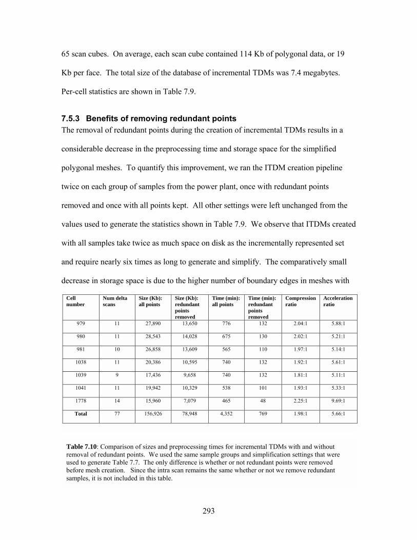
293

65 scan cubes. On average, each scan cube contained 114 Kb of polygonal data, or 19

Kb per face. The total size of the database of incremental TDMs was 7.4 megabytes.

Per-cell statistics are shown in Table 7.9.

7.5.3 Benefits of removing redundant points The removal of redundant points during the creation of incremental TDMs results in a

considerable decrease in the preprocessing time and storage space for the simplified

polygonal meshes. To quantify this improvement, we ran the ITDM creation pipeline

twice on each group of samples from the power plant, once with redundant points

removed and once with all points kept. All other settings were left unchanged from the

values used to generate the statistics shown in Table 7.9. We observe that ITDMs created

with all samples take twice as much space on disk as the incrementally represented set

and require nearly six times as long to generate and simplify. The comparatively small

decrease in storage space is due to the higher number of boundary edges in meshes with

Cell number

Num delta scans

Size (Kb): all points

Size (Kb): redundant points removed

Time (min): all points

Time (min): redundant points removed

Compression ratio

Acceleration ratio

979 11 27,890 13,650 776 132 2.04:1 5.88:1

980 11 28,543 14,028 675 130 2.02:1 5.21:1

981 10 26,858 13,609 565 110 1.97:1 5.14:1

1038 11 20,386 10,595 740 132 1.92:1 5.61:1

1039 9 17,436 9,658 740 132 1.81:1 5.11:1

1041 11 19,942 10,329 538 101 1.93:1 5.33:1

1778 14 15,960 7,079 465 48 2.25:1 9.69:1

Total 77 156,926 78,948 4,352 769 1.98:1 5.66:1

Table 7.10: Comparison of sizes and preprocessing times for incremental TDMs with and without removal of redundant points. We used the same sample groups and simplification settings that were used to generate Table 7.7. The only difference is whether or not redundant points were removed before mesh creation. Since the intra scan remains the same whether or not we remove redundant samples, it is not included in this table.

294

redundant points removed. Recall that the view-dependent simplification stage attempts

to preserve screen-space boundaries to within half a pixel of error. When we remove a

point from a sample, we create a new screen-space boundary that must be preserved.

This limits the ability of the simplification stage to collapse edges that span larger

portions of the scene. Nevertheless, the sixfold improvement in preprocessing time

justifies the expense of identifying and removing redundant points within samples even if

the 50% reduction in storage space is deemed insufficient to compensate for the extra

effort.

7.5.4 Increased fidelity over standard TDMs We claim that the lack of skins in incremental textured depth meshes leads to a higher-

quality reconstruction of the far field than standard, single-source TDMs. Visibility

artifacts in TDMs take the form of skins connecting surfaces that are discontinuous along

the depth dimension. As the user moves farther and farther away from a sample location,

depth discontinuities tend to subtend more of the view, leading to stretching and smearing

as distant pixels are interpolated to cover the hole. ITDMs are constructed to avoid

including skin triangles, instead leaving gaps where no information is available. This

allows us to fill in the holes and thus reduce or eliminate visibility artifacts by rendering

meshes constructed from several different sample locations. By contrast, rendering more

than one standard textured depth mesh in the same view region makes matters worse: not

only do the skins from the first TDM obscure any newly visible surfaces contained in

subsequent meshes, but the skins in subsequent meshes will probably obscure surfaces

that are already rendered properly in the reconstruction! We compare the increasing

fidelity of incremental TDMs with the increasing artifacts in standard TDMs in Figures

295

7.41 through 7.46. Further examples of increasing ITDM fidelity by adding samples to

the reconstruction are shown in Figures 7.50 and 7.51. We also observe that incremental

TDMs can provide a usable (if less than ideal) reconstruction of the far field for

viewpoints well outside the original viewing region containing the input samples. By

contrast, standard TDMs grow rapidly worse outside this region as skins begin to subtend

more of the field of view. This comparison is illustrated in Figure 7.47. One result of

this wider region of fidelity is that the spacing of cells within the environment, which was

previously chosen largely to limit the prevalence of artifacts in the far field, can probably

be increased. This would lead to lower preprocessing and storage costs due to fewer sets

of impostors to generate as well as reduced runtime overhead due to a simpler cell grid

and fewer potentially visible sets (per-cell lists of geometry) that must be stored in main

memory.

296

Figure 7.41: Behavior of standard vs. incremental TDMs as more meshes are rendered in a single reconstruction. This image shows the ideal view (geometry only) for comparison. The five pairs of images that follow show the appearance of incremental TDMs (on the left) and standard single-source-image TDMs (on the right) for one, two, three, four, and five samples, respectively.

Figure 7.42: ITDM vs. TDM, one sample

297

Figure 7.43: ITDM vs. TDM, two samples

Figure 7.44: ITDM vs. TDM, three samples

298

Figure 7.45: ITDM vs. TDM, four samples

Figure 7.46: ITDM vs. TDM, five samples

299

Figure 7.47: Incremental TDMs can provide usable reconstructions in situations where standard TDMs fail badly. Each column of images shows a comparison between geometry only (top), standard TDMs (middle), and incremental TDMS (bottom). These views were acquired three meters from the center of a one-meter-square cell, well outside the region where the impostors were expected to be reasonable approximations of distant geometry.

300

The increased fidelity of incremental TDMs comes at the cost of higher polygon

counts in order to accommodate the geometric portion of multiple incremental TDMs.

As a result, the frame rate of an interactive system is lower with ITDMs than with

standard TDMs. This is illustrated in Figures 7.48 and 7.49. However, the frame rates

we observe with incremental TDMs are still well within interactive ranges (20-40 frames

per second), suggesting that this tradeoff may be acceptable in many situations. In

applications where high frame rates are essential, such as generation of stereo pairs for

head-mounted display, standard TDMs may be a preferable far-field representation.

Like many other simplification- and impostor-based rendering acceleration

techniques, incremental textured depth meshes increase the frame rate at the cost of

visual fidelity. The image-based samples used to construct ITDMs limit the information

initially present in the reconstruction. The processes of redundant sample removal and

0

20

40

60

80

100

120

140

1 123 245 367 489 611 733 855 977 1099 1221 1343 1465 1587 1709 1831

Time (frame number)

Fram

es p

er s

econ

d

Standard TDMs Incremental TDMs

Figure 7.48: Uniformly sampled TDMs produce higher frame rates than incremental TDMs. This is due in part to the different simplification criteria: uniform TDMs are simplified to meet a polygon budget (60,000 triangles per scan cube in this case), whereas incremental TDMs are simplified to meet screen-space error bounds (0.5 pixels at boundaries and silhouettes).

301

view-dependent polygonal simplification further degrade the fidelity of the rendering of

the far field. However, much like static LODs, the incremental nature of our approach

allows the user to trade off the frame rate against increased fidelity by allowing more

scan cubes to be rendered as part of the reconstruction. In Figures 7.50 and 7.51 we show

a scene rendered first with static LODs, then with an increasing number of incremental

textured depth meshes to illustrate this tradeoff.

Figure 7.49: Incremental TDMs consistently use more polygons to render the far field than standard, uniformly sampled TDMs. This results in lower update rates (as shown in Figure 7.47) but fewer reconstruction artifacts due to skins and disocclusions than occur in standard TDMs.

0

50000

100000

150000

200000

250000

300000

350000

400000

1 129 257 385 513 641 769 897 1025 1153 1281 1409 1537 1665 1793

Time (frame number)

Poly

gons

per

fram

e

Standard TDMs Incremental TDMs

302

Figure 7.50 (parts a-d): A view in the house environment as more incremental TDM samples are added. The viewpoint is in the lower right corner of the dependency tree drawn in each image. Red nodes in the tree indicate ITDMs that are being rendered. We see little visual improvement as samples 2, 3, and 4 are added since they cannot see into the bedroom visible through the doors. However, the gaps in the floor visible beyond the door grille at right are being filled in.

(c) Three samples (d) Four samples

(b) Two samples (a) One sample

303

(e) Five samples (f) Six samples

(g) Seven samples (h) Geometry only (ideal view)

Figure 7.50 (parts e-h): Increasing ITDM fidelity by adding more samples to the reconstruction. As samples 5, 6, and 7 are added, the sample location approaches the viewpoint and we see considerable reduction in the holes visible through the bedroom door. Adding more than seven samples contributes little more to the reconstruction in this case. Part (h) shows a geometry-only view for comparison. Individual depth meshes in the house tend to be very small, making it feasible to render several in a single reconstruction.

304

(a) One sample

(d) Four samples (c) Three samples

(b) Two samples

Figure 7.51: Increasing ITDM fidelity in the power plant by adding samples. The viewpoint is in the upper right quadrant of the dependency tree drawn in the lower left corner of each image. These images show reconstructions using one, two, three, and four images, respectively. A geometry-only view is shown on the next page for comparison.

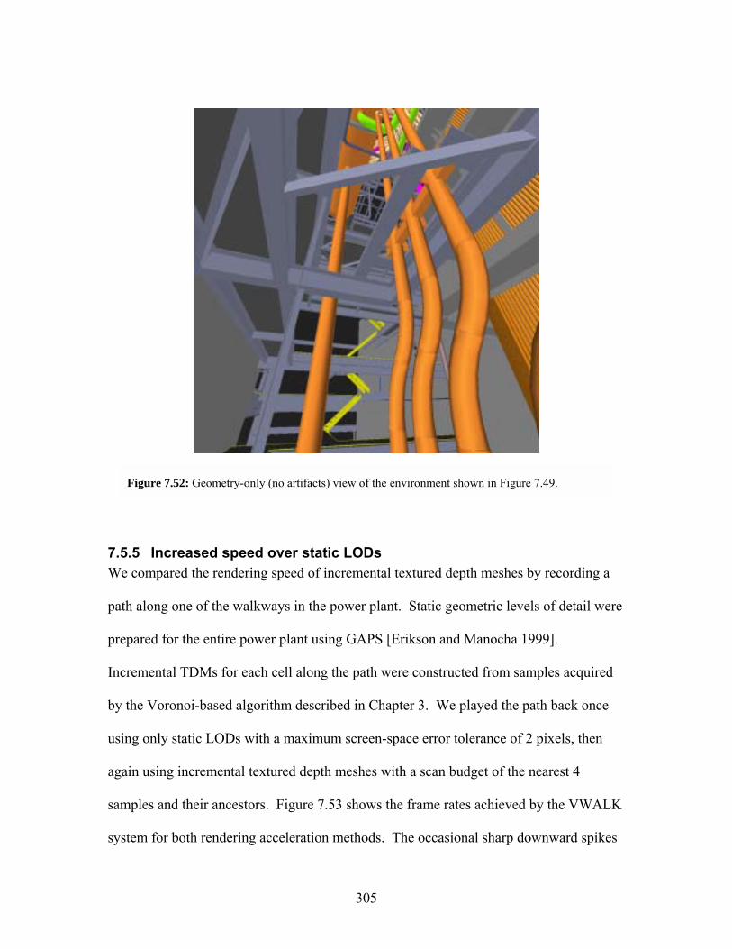
305

7.5.5 Increased speed over static LODs We compared the rendering speed of incremental textured depth meshes by recording a

path along one of the walkways in the power plant. Static geometric levels of detail were

prepared for the entire power plant using GAPS [Erikson and Manocha 1999].

Incremental TDMs for each cell along the path were constructed from samples acquired

by the Voronoi-based algorithm described in Chapter 3. We played the path back once

using only static LODs with a maximum screen-space error tolerance of 2 pixels, then

again using incremental textured depth meshes with a scan budget of the nearest 4

samples and their ancestors. Figure 7.53 shows the frame rates achieved by the VWALK

system for both rendering acceleration methods. The occasional sharp downward spikes

Figure 7.52: Geometry-only (no artifacts) view of the environment shown in Figure 7.49.

306

in the frame rate for incremental textured depth meshes occur when the system binds

several texture maps at once. These spikes could be evened out by binding a texture in

several smaller chunks (similar to speculative prefetching of model data) instead of as

one large image. Moreover, there is significant variation in the frame rate shown by

ITDMs, from 20 frames per second around texture binding times to over 40 in some

places. This variation is due to fine-grained view frustum culling of depth meshes. Such

culling is possible because of the resampling that takes place during ITDM generation,

when long, thin triangles that can span the entire height of the power plant (as in the

furnace) are broken up into many smaller ones. We observe that incremental textured

depth meshes permit an interactive frame rate even in situations where the user is looking

toward regions of dense, complex geometry that reduce static LODs to two or three

frames per second. Figure 7.54 compares the number of polygons rendered by

incremental TDMs and static LODs for each frame along the path.

307

0

10

20

30

40

50

60

1 201 401 601 801 1001 1201 1401 1601

Incremental TDMs Static LODs

Figure 7.53: Frame rate comparison between incremental TDMs and static levels of detail along a path in the power plant. ITDMs were generated using the algorithms described in chapters 3 and 6. Static LODs were generated using GAPS [Erikson and Manocha 1999]. At runtime, we rendered ITDMs with a fidelity budget of 4 nearby scans and compared them with static LODs rendered at 2 pixels of screen-space error.

308

0

500000

1000000

1500000

2000000

2500000

3000000

3500000

1 251 501 751 1001 1251 1501 1751

Time (frame number)

Poly

gons

per

fram

e

Static LODs Increm ental TDMs

Figure 7.54: Polygon counts for both static LODs and incremental TDMs along a path through the power plant

8 Conclusions and Future Work

8.1 Introduction

In this dissertation we have presented rendering acceleration techniques for

interactive walkthroughs of complex synthetic environments. These techniques are based

around the idea of simplifying parts of a complex geometric environment by replacing

distant primitives with image-based samples, then further simplifying those samples

using spatial encoding techniques that result in compact, easy-to-render representations.

The samples forming the initial image-based simplification are acquired using an

incremental search for the best next view based on the Voronoi diagram of the locations

of existing samples. We encode the image and geometric portions of these samples

separately to construct a set of impostors. The image-space component of the impostors

consists of a database of spatially encoded video, which is a generalization of MPEG-2

video compression that allows the representation of a 3D space of images instead of a 1D

temporal sequence. The geometric component of the impostors is represented as a set of

incremental textured depth meshes. These meshes are created by removing redundant

points from samples of the environment, then simplifying a dense polygonal mesh

created from the remaining points. By dividing the available rendering capacity between

nearby primitives and distant, simplified impostors, we are able to maintain interactive

update rates while rendering nearby primitives at high fidelity. These algorithms result in

310

more efficient allocation of resources than with the uniformly spaced sample locations

used in previous work.

We have presented a system for interactive exploration of complex synthetic

environments based around the idea of cell-based walkthrough. This system begins with

a regular subdivision of some navigable region into rectangular cells. For each of these

cells, we compute the maximum extent of a concentric cull box containing fewer than

some threshold number of primitives. At runtime, the primitives inside the cull box (the

near field) are rendered using original data or some high-fidelity approximation such as

static geometric levels of detail. The methods presented in this dissertation focus on

representations for the far field composed of all primitives outside the cull box.

8.1.1 Simplifying complex environments with image-based samples The construction of far-field impostors begins with the acquisition of a set of

panoramic samples of the environment for each cell. This allows us to replace complex

geometry with a simpler image-based representation. Samples should be placed to

capture as many of the surfaces potentially visible from within the cell as possible. An

optimal placement for a group of viewpoints to survey the environment visible from a

region is difficult to compute: in fact, it is closely related to the classical art gallery

problem. This suggests that positioning a minimum number of viewpoints for a given

view region is likely to be NP-hard. Rather than tackle this problem, we have proposed

an incremental sampling scheme that places new sample viewpoints along the 2D

Voronoi diagram of the locations of the existing samples. The advantage of Voronoi-

based sampling over randomized methods or brute-force search is that it describes those

points that are farthest from the existing sample locations. We expect that the farther

311

away two points are, the less their views of an environment will have in common:

therefore, Voronoi sites should tend to reveal objects previously unseen from any sample

location. This sampling process continues until an estimate of the maximum error for

any point in the view region falls below a user-specified threshold.

8.1.2 Spatial encoding of image-space simplifications The image-based samples acquired by the incremental Voronoi-based sampling

algorithm are further simplified to produce a set of impostors. These impostors have both

image-space and geometric components and are encoded using spatial relationships

present within the database of samples. The image and geometric components of

impostors can each be considered as representations of parts of the input database.

Moreover, our algorithms for spatial encoding share a common structure. The particular

properties of an impostor representation vary according to the nature of the operations

comprising this structure. These operations include the following:

1. Compare groups of sample elements from two separate

samples of the environment. This allows the detection of

redundant information present in more than one sample.

2. Remove or alter groups of sample elements within a single

sample. This allows the removal of data identified as redundant or

its transformation into a form more suitable to compact

representation.

3. Establish a hierarchy over a set of samples. In order to identify

and remove redundant data, we need some notion of precedence: if

two sample elements belong to the same point on the same surface

312

in the environment, a hierarchy allows us to decide which element

to keep and which to discard.

8.1.3 Spatial video encoding The samples of the environment exhibit considerable coherence in the surfaces

captured in each one. Such coherence can be detected and exploited by video

compression techniques. We have described two separate representations for the

database of samples based on the structure of MPEG2 video.

8.1.3.1 Strict compatibility with standard MPEG2 video The first spatial video representation presented maintains strict compatibility with

existing MPEG2 encoders and decoders by arranging the 3-dimensional space of samples

into 1-dimensional sequences of images. Standard image-space search algorithms are

used to estimate motion vectors. Moreover, the structure of the video stream (including

the length and composition of each group of pictures) is not altered to respond to the

characteristics of the environment. As a result, compression artifacts tended to appear

more severe in places where the 1D sequence of images is a poor match for the structure

of the 3D space of images. The dependency structure between frames in a single group

of pictures also often required several frames to be decoded when the user moved from

one cell to an adjacent one. Nonetheless, compatibility with existing tools allowed us to

take advantage of heavy optimizations performed in those tools, thus enabling efficient

decoding and display of the compressed images at runtime.

8.1.3.2 Direct spatial encoding of 3D cell structure By abandoning strict compatibility with existing MPEG2 tools, we devised a

spatial video representation that more directly represented the 3D nature of the input

313

database. Instead of indexing images and dependencies along a single temporal

dimension, a spatially encoded video database does not assume any particular structure

among its input images: as a result, a 3D grid or even a 4D time-varying sequence can be

represented as easily as a 1D sequence. By matching inter-frame dependencies to spatial

locations in the input database, we increased the chances of finding a good match during

motion compensation. Moreover, by exploiting camera information and per-pixel depth

during the encoding process, we significantly reduced the cost of motion-vector search,

traditionally one of the most expensive parts of video encoding.

8.1.4 Incremental textured depth meshes In order to use the spatial video databases as far-field impostors, we must provide

geometry onto which the images can be projected. We have presented an incrementally

constructed variant of standard textured depth meshes that reduces the artifacts present in

many previous systems while increasing the range of viewpoints for which a faithful

approximation of the far field is possible. This representation can be seen as a geometric

simplification of the image-based samples acquired by the incremental sampling

algorithm described above. We reduce the storage requirements and rendering overhead

of incremental textured depth meshes by establishing a dependency tree over a group of

samples. Each sample is modified to contain only those surfaces that are not present in

any of its ancestors. As a result, the sample corresponding to the root of the tree is

rendered using all of its sample elements, whereas its children typically contribute only a

small fraction of the overall reconstruction. We further reduce the rendering cost using

view-dependent simplification techniques that take advantage of the limited view volume

and view directions for any given set of TDMs.

314

8.2 Future Work

We have encountered many avenues for future work. In this section we describe

a few such avenues.

8.2.1 Sampling the Environment Several avenues for improvements to the incremental sampling algorithm present

themselves. Foremost among them is the construction of candidate viewpoints: whereas

relatively simple environments converge quickly to a near-complete sampling of visible

surfaces, configurations with large occluders with complex interactions can be

problematic. Approximate visibility techniques such as those employed in hierarchical

radiosity might yield a relatively inexpensive way to compute better candidate viewpoints.

We conjecture that such techniques might be an efficient way to identify a small set of

points that see a large portion of the environment. This is similar to the method described

by Stuerzlinger [1999]. This small set of viewpoints could be used as a set of initial

sample locations followed by Voronoi-based sampling to fill in the gaps, or the

approximate visibility method could be used to generate all sample locations.

Second, the evaluation of the visible extent of the void surface currently involves

one read-back of the OpenGL stencil buffer for each sample. This can grow expensive in

environments where many samples have been acquired, particularly in systems where the

bandwidth between the CPU and the graphics pipeline is a bottleneck (i.e. most PC

hardware currently available). It should be possible to construct the stencil buffer

operations to allow the per-pixel skin count to be computed using a single readback for

an entire set of skins instead of reading the buffer for every separate sample added to the

reconstruction.

315

Third, the current criterion for sampling gives a binary result concerning whether

or not any surface is visible at a certain point. Methods employed in other best-next-view

systems to ensure a certain minimum sampling resolution or a minimum angle of

incidence may be able to increase the quality of the reconstruction. Finally, an early

rejection test could prove useful by allowing us to avoid computing visibility error in

regions of the environment that are already well sampled.

Although the sampling pattern within each region is guided by our approximate

visibility algorithms, the layout of the regions themselves is still the same uniform grid

used in systems such as [Aliaga et al. 1999]. Since our spatially encoded impostor

representation produces acceptable results over much wider regions than single-source

textured depth meshes constructed from the same samples, it should be possible to

construct a smaller set of larger view regions. Moreover, the uneven distribution of

primitives within an environment suggests that the sizes of the regions themselves can be

adapted to better concentrate the effort required by image-space simplification in regions

of high complexity.

8.2.2 Spatial Video Encoding We observed better results with a direct encoding of the spatial structure of the

input database than with the strict-compatibility video scheme. Nevertheless, there exist

opportunities to improve upon both approaches. There are several optimizations

(described below) that might allow a standard MPEG2 stream to better fit the properties

of a sampled environment and hence yield better encodings.

316

8.2.2.1 Improvements to the strict-compatibility representation Some of the shortcomings of a spatial video representation strictly compatible

with MPEG2 video can be addressed by changing the mapping from the 2D layers of the

database of environment maps to a 1D sequence of images. A row-major ordering results

in adjacent cells in different rows of the grid being placed far apart in the MPEG streams.

A more useful ordering would do a better job of preserving spatial locality by increasing

the number of cases in which frames taken from environment maps close to one another

in the original database are placed close together in the video streams. The space-filling

curve first described by Hilbert in 1891 [Hilbert 1891, Peitgen and Saupe 1988 pp.

278,284] (see Fig. 8.1) can provide such an ordering, as it maps points that are close

together in space onto points that are close together in the 1D domain of the curve.

Figure 8.1 shows a possible ordering of frames based on such a curve. Although there

are still discontinuities in such a mapping where adjacent cells are far apart in the video

stream, each group of pictures spans a 2D area within which the user can navigate

without forcing random frame accesses to different groups of pictures. In environments

where the 3D environment cannot be cleanly separated into 2D layers, a 3-dimensional

analogue of the 2D Hilbert curve may be applicable.

317

Adapting the structure of the group of pictures (GOP) and the motion vectors to

better suit the model will require changes to the encoder to make it aware of extra

information about the data being represented. Since motion prediction fails when there is

no coherence between the predictive base and the frame being encoded (as is the case

when the viewpoint passes through a wall), access to model information would allow the

encoder to identify such cases and begin a new GOP instead of trying to continue the

existing one. Moreover, camera information plus per-pixel depth in the original

environment maps allows us to compute exact motion vectors for each pixel. It may be

possible to accelerate the encoding process by modifying the encoder to use the same sort

of motion-vector prediction described in Section 4.2.3.2. Since these changes do not

change the format of the output of the encoder, only its quality, we maintain the desired

compatibility with standard MPEG decoders.

1 2

4 3

5 8

6 7

9 12

10 11

15 16

14 13

59 58

60 57

61 62

64 63

51 52

50 49

55 54

56 53

33 36

34 35

47 46

48 45

41 42

44 43

37 38

40 39

17 20

18 19

31 30

32 29

25 26

28 27

21 22

24 23

Figure 8.1: An ordering of a square grid of cells based on a Hilbert curve. Such an ordering better preserves spatial locality in the 2D-grid-to-1D-stream 1D mapping than a simple row-major ordering of the cells.

318

8.2.2.2 Better encodings of synthetic environments Our experiences while applying MPEG2-style compression to images of synthetic

environments have emphasized that the MPEG standard was developed with natural

imagery in mind. Synthetic images often contain large areas of low spatial frequency

(particularly in diffusely lit environments) bordered by very sharp edges. These are

precisely the frequencies that are considered unimportant by the quantization matrix!

Moreover, the 8x8 discrete cosine transform is by definition unable to capture

frequencies whose wavelength falls outside the range of 2 to 16 pixels. It may be

possible to construct a more appropriate quantization matrix for synthetic imagery by

examining the spectra of a large number of representative images. The interested reader

is referred to [Watson 1994] for more information. It may also be the case that a different

basis transformation such as the discrete wavelet transform used in JPEG2000 [Taubman

and Marcellin 2001] is better able to approximate synthetic imagery. In particular, the

process of redundant sample removal tends to increase the high frequency content of an

image. This pushes the data set closer to difficult cases for the discrete cosine transform.

It might be interesting to explore the limits of the compression our methods can

achieve. Whereas the compression ratio tends to increase as a function of the degree of

coherence between the predictive base and the frame being encoded, each frame carries

with it a fixed overhead. Denser sampling may increase coherence between nearby

images, but there must exist a point at which the fixed overhead dominates any increased

compression. This point is likely to be model-dependent. Moreover, the expense of

acquiring and storing samples of the original environment is likely to grow prohibitive

long before we reach this maximum useful density. Characterizing the maximum

achievable compression and the maximum useful sample density in relation to the

319

properties of an environment could allow us to design termination conditions for

Voronoi-based sampling that obey limits on the size of the compressed impostor database.

8.2.3 Incremental textured depth meshes Two avenues for future work with incremental TDMs involve the simplification

scheme and the treatment of small holes in the original dense mesh. Since most of the

problem cases identified in Section 5.4.2 are a result of faithful preservation of high-

frequency detail independent of the user�s viewpoint, we may be able to benefit from

using samples from nearby scans to fill in these holes and enable a much more drastic

simplification. The resulting rendering artifacts could be reduced or eliminated by

rendering TDMs known to contain correct information on top of these filled-in, possibly

incorrect gaps. In synthetic environments where object identifiers are available, we could

identify such TDMs during preprocessing by searching for surfaces coincident with the

borders of the gap that share the same identifiers.

Moreover, we may be able to extend the view-dependent simplification scheme to

preserve these boundaries only when the user can actually see them. Recent work in

region-based occlusion culling for polygonal environments delineates several promising

approaches. In fact, it may be possible to eliminate large parts of textured depth meshes

by considering the occlusion patterns of the near field. Regions exist in both the house

and power plant environments where a wall in the near field completely occludes the far

field over a wide field of view. If we can detect such configurations, we need not even

acquire samples in those directions, let alone construct incremental TDMs for those

portions of the view.

320

Surfaces that are represented piecewise across multiple meshes in a set of ITDMs

are another difficult case. In order to prevent cracks from appearing at the seams

between different pieces of a single surface, we make a particular effort to preserve the

screen- and world-space boundaries of such pieces. Our current simplification methods

preserve these boundaries by restricting the permissible screen-space simplification error

to at most half a pixel along image-space silhouettes. This can lead to situations where

many polygons are used to represent a smooth, flat surface. Better results might be

achieved with a simplification method that can operate across the several meshes that

comprise a single object, in effect �zippering� the boundaries together to allow a

simplification with fewer polygons. Turk and Levoy [1994] apply such an approach to

create watertight meshes from a set of registered range images. Such methods are likely

to produce meshes that extend across the screen-space boundaries we currently preserve.

However, we conjecture that this over-extension will not be a major problem.

Connecting the pieces of surfaces present in different samples is analogous to filling in

gaps in a surface within a single sample. The same methods (described above in Section

8.2.3) might therefore be applicable in both situations.

Finally, we note that there is considerable information present in the points we

currently discard as redundant. At present, our criterion for identifying a point as

redundant only considers whether that point is co-planar with the (estimated) surface in

some other sample. We do not account for the resolution at which the surface is sampled

or the angle of incidence between the eye ray and the surface in question. Both of these

factors can affect the amount of information present in a given sample regarding a given

surface. If some particular surface is sampled at a grazing angle in an intra scan and

321

head-on in some delta scan, the delta scan is likely to contain more information about the

position and texture of the surface in question. We might be able to capture more

information about the geometry of the surface by reallocating the delta scan�s samples of

that surface to the intra scan instead of discarding them immediately. Similarly, if we

reallocate so-called redundant samples to the scan cube where a particular surface is

represented, we could build multiresolution texture maps of that surface to allow a

faithful reconstruction of surface detail over a wider range of viewing directions and

distances. Finally, �redundant� samples that fall near an image-space boundary could be

used to improve the reconstruction of such boundaries by providing more information

than was present in the original sample.

322

BIBLIOGRAPHY

[Adelson and Bergen 1991] E.H. Adelson and J.R. Bergen. "The Plenoptic Function and

the Elements of Early Vision". In Computational Models of Visual Processing. eds Landy, M. & J.A. Movshon. Cambridge, Massachusetts: MIT Press, 1991.

[Aggarwal 1984] A. Aggarwal. "The art gallery theorem: Its variations, applications, and algorithmic aspects". Ph.D. dissertation, The Johns Hopkins University, Baltimore, MD.

[Agrawala et al. 1995] M. Agrawala, A. Beers and N. Chaddha. "Model-based motion estimation for synthetic animations". In Proceedings of Third ACM International Conference on Multimedia. pp. 477-488 ACM Press, 1995

[Airey 1990] J. Airey. "Increasing Update Rates in the Building Walkthrough System with Automatic Model-Space Subdivision and Potentially Visible Set Calculations". In Department of Computer Science. Chapel Hill, North Carolina: University of North Carolina at Chapel Hill.

[Airey et al. 1990] J. Airey, J. Rohlf and F.P. Brooks, Jr. "Towards image realism with interactive update rates in complex virtual building environments". In Proceedings of 1990 ACM Symposium on Interactive 3D Graphics. pp. 41-50 ACM Press, 1990

[Aliaga 1999] D. Aliaga, J. Cohen, A. Wilson, E. Baker, H. Zhang, C. Erikson, K. Hoff, T. Hudson, W. Stuerzlinger, R. Bastos, M. Whitton, F.P. Brooks, Jr., and D. Manocha. "MMR: An Integrated Massive Model Rendering System using Geometric and Image-Based Acceleration". In Proceedings of ACM Symposium on Interactive 3D Graphics ACM Press, 1999

[Aliaga and Lastra 1997] D. Aliaga and A. Lastra. "Architectural Walkthroughs using Portal Textures". In Proceedings of IEEE Visualization 1997. pp. 355-362 IEEE Press, 1997

[Aliaga and Lastra 1999] D. Aliaga and A. Lastra. "Automatic image placement to provide a guaranteed frame rate". In Proceedings of ACM SIGGRAPH 1999. pp. 307-316, Los Angeles, CA, ACM Press, 1999

324

[Allen et al. 1998] P. Allen, M. Reed and I. Stamos. "View planning for site modeling". In Proceedings of DARPA Image Understanding Workshop. pp. 1181-1192, Monterey, California, 1998

[Banta et al. 2000] C.J. Banta, L. Wong, C. Dumont and M.A. Abidi. "A next-best-view system for autonomous 3D object reconstruction". IEEE Transactions on Systems, Man and Cybernetics, 3:5, 589-598.

[Banta et al. 1995] J.E. Banta, Y. Zhien, X.Z. Wang, G. Zhang, M.T. Smith and M.A. Abidi. "A "best-next-view" algorithm for three dimensional scene reconstruction using range images". In Proceedings of SPIE Conf. on Intelligent Robots and Computer Vision. pp. 418-429, 1995

[Baxter et al. 2002] B. Baxter, A. Sud, N. Govindaraju and D. Manocha. "GigaWalk: Interactive walkthrough of complex environments". In Proceedings of Eurographics Workshop on Rendering 2002, Pisa, Italy, 2002

[Berc et al. 1996] L. Berc, W. Fenner, R. Frederick and S. Mccanne. "RTP payload format for JPEG-compressed video". Internet RFC 2035, IETF, 1996

[Besl and McKay 1992] P.J. Besl and N.D. Mckay. "A method for registration of 3-D shapes". IEEE Transactions on Pattern Analysis and Machine Intelligence, 14:2, 239-256, 1992.

[Bhaskaran and Konstantinides 1997] V. Bhaskaran and K. Konstantinides. Image and video compression standards. Norwell, Massachusetts: Kluwer Academic Publishers, 1997.

[Bjorling-Sachs and Souvaine 1995] I. Bjorling-Sachs and D.L. Souvaine. "An efficient algorithm for guard placement in polygons with holes". Discrete Computational Geometry, 13, 77-109, 1995.

[Blinn and Newell 1976] J.F. Blinn and M.E. Newell. "Texture and reflection in computer generated images". Communications of the ACM, 19:10, 542-547, 1976

[Boutell 1997] T. Boutell. "PNG (Portable Network Graphics) Specification". In RFC 2083: IETF (Internet Engineering Task Force).

[Carraro et al. 1998] G. Carraro, J. Edmark and J.R. Ensor. "Techniques for handling video in virtual environments". In Proceedings of ACM SIGGRAPH 1998. pp. 353-360, Orlando, Florida, ACM Press, 1998

325

[Catmull 1975] E. Catmull. "Computer display of curved surfaces". In Proceedings of Conf. on Computer Graphics, Pattern Recognition, and Data Structure. pp. 11-17, 1975

[Catmull 1974] E. Catmull. "A Subdivision Algorithm for Computer Display of Curved Surfaces". Ph.D. dissertation, University of Utah, Salt Lake City, Utah 1974.

[Chai et al. 2000] J.-X. Chai, S.-C. Chan, H.-Y. Shum and X. Tong. "Plenoptic sampling". In Proceedings of ACM SIGGRAPH 2000. pp. 307-318, New Orleans, Louisiana, ACM Press, 2000

[Chang et al. 1999] C.-F. Chang, G. Bishop and A. Lastra. "LDI tree: a hierarchical representation for image-based rendering". In Proceedings of ACM SIGGRAPH 1999, Los Angeles, California, ACM Press, 1999

[Clark 1976] J. Clark. "Hierarchical geometric models for visible surface algorithms". In Communications of the ACM. 19:10, pp. 547-554, 1976.

[Conolly 1985] C.I. Conolly. "The determination of next best views". In Proceedings of International Conference on Robotics and Automation. pp. 432-435, 1985

[Curless and Levoy 1996] B. Curless and M. Levoy. "A volumetric method for building complex models from range images". In Proceedings of ACM SIGGRAPH 1996. pp. 303-312, Orlando, Florida, ACM Press, 1996

[Daly 1993] S. Daly. "The visible differences predictor: an algorithm for the assessment of image fidelity". In Digital Images and Human Vision. ed Watson, A. pp. 179-206. Cambridge, Massachusetts: MIT Press, 1993.

[Darsa 1998] L. Darsa, B. Costa, and A. Varshney. "Walkthroughs of complex environments using image-based simplification". Computers and Graphics, 22:1, pp. 55-69, 1998.

[Darsa et al. 1997] L. Darsa, B. Costa Silva and A. Varshney. "Navigating static environments using image-space simplification and morphing". In Proceedings of 1997 ACM Symposium on Interactive 3D Graphics. pp. 25-34, ACM Press, 1997

[Debevec et al. 1996] P. Debevec, C. Taylor and J. Malik. "Modeling and Rendering Architecture from Photographs: A Hybrid Geometry- and Image-Based Approach". In Proceedings of ACM SIGGRAPH 1996. pp. 11-20, New Orleans, Louisiana, ACM Press, 1996

326

[Decoret et al. 2002] X. Decoret, F. Durand, F. Sillion and J. Dorsey. "Billboard clouds". Research report RR-4485, INRIA, Montbonnot-St-Martin, France, June 2002, 2002

[Decoret et al. 1999] X. Decoret, G. Schaufler, F. Sillion and J. Dorsey. "Multi-layered impostors for accelerated rendering". In Proceedings of Eurographics 1999. ed. Scopigno, R. & P. Brunet, Milano, Italy, 1999

[Durand et al. 1996] F. Durand, G. Drettakis and C. Puech. "The 3D visibility complex: A new approach to the problem of accurate visibility". In Proceedings of Eurographics Rendering Workshop 1996. ed. Schroeder, P. and Pueyo, X., pp. 245-256, New York, Springer Verlag, 1996

[Durand et al. 2000] F. Durand, G. Drettakis, J. Thollot and C. Puech. "Conservative visibility preprocessing using extended projections". In Proceedings of ACM SIGGRAPH. pp. 239-248, New Orleans, Louisiana, ACM Press, 2000

[Ebrahimi and Pereira 2002] T. Ebrahimi and F. Pereira. "The MPEG-4 Book". pp. 887: Prentice Hall, 2002.

[Eck et al. 1995] M. Eck, T. Derose, T. Duchamp, H. Hoppe, M. Lounsbery and W. Stuetzle. "Multiresolution analysis of arbitrary meshes". In Proceedings of ACM SIGGRAPH 1995. pp. 173-182 ACM Press, 1995

[Erikson and Manocha 1999] C. Erikson and D. Manocha. "GAPS: General and Automatic Polygonal Simplification". In Proceedings of 1999 ACM Symposium on Interactive 3D Graphics. pp. 79-88 ACM Press, 1999

[Foley et al. 1990] J. Foley, A. Van Dam, S. Feiner and J. Hughes. Computer Graphics: Principles and Practice. Reading, Massachusetts: Addison Wesley, 1990.

[Funkhouser 1996] T. Funkhouser, S. Teller, C. Sequin, and D. Khorramabadi. "The UC Berkeley System for Interactive Visualization of Large Architectural Models". Presence, 5:1, 1996.

[Funkhouser et al. 1992] T. Funkhouser, C. Sequin and S. Teller. "Management of large amounts of data in interactive building walkthroughs". In Proceedings of 1992 ACM Symposium on Interactive 3D Graphics. pp. 11-20. 1992

[Garland 1998] M. Garland, and Heckbert, Paul. "Simplifying surfaces with color and texture using quadric error metrics". In Proceedings of IEEE Visualization 1998. pp. 263-269 IEEE Press, 1998

327

[Garland and Heckbert 1997] M. Garland and P. Heckbert. "Surface Simplification using Quadric Error Metrics". In Proceedings of ACM SIGGRAPH 1997. pp. 189-198, Los Angeles, California, ACM Press, 1997

[GIF89a 1990] Gif89a. "GIF89a Specification": CompuServe, Inc.

[Gigus 1991] Z. Gigus, J. Canny, and R. Seidel. "Efficiently computing and representing aspect graphs of polyhedral objects". IEEE Transactions on Pattern Matching and Machine Intelligence, 13:6, 1991.

[Gigus and Malik 1990] Z. Gigus and J. Malik. "Computing the aspect graph for the line drawings of polyhedral objects". IEEE Transactions on Pattern Matching and Machine Intelligence, 12:2, 1990.

[Gortler et al. 1996] S. Gortler, R. Grzeszczuk, R. Szeliski and M. Cohen. "The Lumigraph". In Proceedings of ACM SIGGRAPH 1996. pp. 43-54, New Orleans, Louisiana, ACM Press, 1996

[Greene et al. 1993] N. Greene, M. Kass and G. Miller. "Hierarchical Z-buffer visibility". In Proceedings of ACM SIGGRAPH 1993. pp. 231-238 ACM Press, 1993

[Haskell et al. 1997] B. Haskell, A. Prui and A. Netravali. Digital Video: An introduction to MPEG-2. New York: Chapman and Hall, 1997.

[Heckbert 1986] P. Heckbert. "Survey of Texture Mapping". IEEE Computer Graphics and Applications November 1986, 56-67, 1986.

[Hilbert 1891] D. Hilbert. "Uber die stetige Abbildung einer Linie auf ein Flachenstueck". Math. Ann., 38, 459-460.

[Hoffmann et al. 1991] F. Hoffmann, M. Kauffman and K. Kriegel. "The art gallery theorem for polygons with holes". In Proceedings of 32nd Symposium of Foundations of Computer Science. pp. 39-48, 1991

[Honsberger 1976] R. Honsberger. Mathematical Gems II. Cambridge University Press, 1976.

[Hoppe 1996] H. Hoppe. "Progressive Meshes". In Proceedings of ACM SIGGRAPH 1996. pp. 99-108, New Orleans, Louisiana, ACM Press, 1996

328

[Hoppe 1997] H. Hoppe. "View-dependent refinement of progressive meshes". In Proceedings of ACM SIGGRAPH 1997. pp. 189-198, Los Angeles, California, ACM Press, 1997

[Isaksen et al. 2000] A. Isaksen, L. Mcmillan and S. Gortler. "Dynamically reparameterized light fields". In Proceedings of ACM SIGGRAPH. pp. 297-306, New Orleans, Louisiana, ACM Press, 2000

[Jain and Jain 1981] J.R. Jain and A.K. Jain. "Displacement measurement and its application in interframe image coding". IEEE Trans. Commun., COM-29:12, 1799-1808.

[Jeschke and Wimmer 2002] S. Jeschke and M. Wimmer. "Layered environment-map impostors for arbitrary scenes". In Proceedings of Graphics Interface 2002, Calgary, Alberta, Canada, 2002

[Jeschke and Wimmer 2002] S. Jeschke and M. Wimmer. "Textured depth meshes for real-time rendering of arbitrary scenes". In Proceedings of 2002 Eurographics Workshop on Rendering, Pisa, Italy, 2002

[Klein and Sequiera 2000] K. Klein and V. Sequiera. "View Planning for the 3D Modelling of Real World Scenes". In Proceedings of 2000 IEEE/RSJ International Conference on Intelligent Robots and Systems, Takaatsu, Japan, IEEE, 2000

[Koenderink and van Doorn 1979] J.J. Koenderink and A.J. Van Doorn. "The internal representation of solid shape with respect to vision". BioCyber, 32, 211-216, 1979.

[Koenderink and van Doorn 1976] J.J. Koenderink and A.J. Van Doorn. "The singularities of the visual mapping". BioCyber, 24(1), 51-59, 1976.

[Kumar et al. 1997] S. Kumar, D. Manocha, H. Zhang and K.E. Hoff, Iii. "Accelerated walkthrough of large spline models". In Proceedings of 1997 ACM Symposium on Interactive 3D Graphics ACM Press, 1997

[Lempel and Ziv 1977] A. Lempel and J. Ziv. "A universal algorithm for sequential data compression". IEEE Transactions on Information Theory, 23:3, 337-343, 1977.

[Levoy 1995] M. Levoy. "Polygon-assisted JPEG and MPEG compression of synthetic images". In Proceedings of ACM SIGGRAPH. pp. 21-30 ACM Press, 1995

329

[Levoy and Hanrahan 1996] M. Levoy and P. Hanrahan. "Light field rendering". In Proceedings of ACM SIGGRAPH. pp. 31-42, New Orleans, Louisiana, ACM Press, 1996

[Lindholm et al. 2001] E. Lindholm, M. Kilgard and H. Moreton. "A user-programmable vertex engine". In Proceedings of SIGGRAPH 2001. pp. 149-157, Los Angeles, California, ACM Press, 2001

[Lippman 1980] A. Lippman. "Movie-Maps: An application of the optical video-disc to computer graphics". In Proceedings of ACM SIGGRAPH 1980 ACM Press, 1980

[Luebke 1997] D. Luebke, and C. Erikson. "View-dependent simplification of arbitrary polygonal environments". In Proceedings of ACM SIGGRAPH. pp. 199-208, Los Angeles, California, ACM Press, 1997

[Luebke and Georges 1995] D. Luebke and C. Georges. "Portals and Mirrors: Simple, Fast Evaluation of Potentially Visible Sets". In Proceedings of 1995 ACM Symposium on Interactive 3D Graphics ACM Press, 1995

[Maciel and Shirley 1995] P. Maciel and P. Shirley. "Visual navigation of large environments using textured clusters". In Proceedings of 1995 ACM Symposium on Interactive 3D Graphics, Monterey, California, ACM Press, 1995

[Mark 1999] W. Mark. "Post-Rendering 3D Image Warping: Visibility, Reconstruction, and Performance for Depth-Image Warping". Ph.D. dissertation, Department of Computer Science, University of North Carolina at Chapel Hill.

[Maver and Bajcsy 1993] J. Maver and R. Bajcsy. "Occlusions as a guide for planning the next best view". IEEE Transactions on Pattern Analysis and Machine Intelligence, 15:5, 417-433, 1993.

[McAllister et al. 1999] D. Mcallister, L. Nyland, V. Popescu, A. Lastra and C. Mccue. "Real-time rendering of real-world environments". Technical report TR99-019, Departmenf of Computer Science, University of North Carolina at Chapel Hill, Chapel Hill, North Carolina, 1999

[McCool et al. 2001] M. Mccool, J. Ang and A. Ahmad. "Homomorphic factorization of BRDFs for high-performance rendering". In Proceedings of ACM SIGGRAPH 2001. pp. 171-178, Los Angeles, California, ACM Press, 2001

[McMillan and Bishop 1995] L. Mcmillan and G. Bishop. "Plenoptic modeling: an image-based rendering syste". In Proceedings of ACM SIGGRAPH 1995. pp. 39-46 ACM Press, 1995

330

[Mitchell et al. 1996] J. Mitchell, W. Pennebaker, C. Fogg and D. Legall. MPEG Video Compression Standard. New York: Chapman and Hall, 1996.

[MPEG-2 1994] I. Mpeg-2, Iso/Iec. Generic coding of moving pictures and associated audio. 1994.

[Olano and Lastra 1998] M. Olano and A. Lastra. "A shading language on graphics hardware: the PixelFlow Shading System". In Proceedings of ACM SIGGRAPH 1998. pp. 159-168, Orlando, Florida, ACM Press, 1998

[Oliveira and Bishop 2000] M. Oliveira and G. Bishop. "Relief texture mapping". In Proceedings of ACM SIGGRAPH 2000. pp. 359-368, New Orleans, Louisiana, ACM Press, 2000

[OpenGL ARB 1992] Opengl Architecture Review Board. OpenGL Reference Manual. Reading, Massachusetts: Addison Wesley, 1992.

[OpenGL ARB 1992] Opengl Architecture Review Board. OpenGL Reference Manual. Reading, Massachusetts: Addison-Wesley, 1992.

[O'Rourke 1998] J. O'Rourke. Computational geometry in C. New York, NY: Cambridge University Press, 1998.

[O'Rourke and Supowit 1983] J. O'Rourke and K. Supowit. "Some NP-hard polygon decomposition problems". IEEE Transactions on Information Theory, 29, 181-190, 1983.

[Peercy et al. 2000] M. Peercy, M. Olano, J. Airey and P.J. Ungar. "Interactive multi-pass programmable shading". In Proceedings of ACM SIGGRAPH 2000. pp. 425-432, New Orleans, Louisiana, ACM Press, 2000

[Peitgen and Saupe 1988] H.-O. Peitgen and D. Saupe. The Science of Fractal Images. New York: Springer-Verlag, 1988.

[Pennebaker and Mitchell 1992] W. Pennebaker and J. Mitchell. JPEG: Still Image Data Compression Standard. Kluwer Academic Publishers, 1992.

[Pito and Bajcsy 1995] R. Pito and R. Bajcsy. "A solution to the next best view problem for automated CAD model acquisition of free-form objects using range cameras". In Proceedings of SPIE Symposium on Intelligent Systems and Advanced Manufacturing, Philadelphia, Pennsylvania, 1995

331

[Pocchiola and Vegter 1996] M. Pocchiola and G. Vegter. "Topologically sweeping visibility complexes via pseudotriangulations". GEOMETRY: Discrete and Computational Geometry, 16, 1996.

[Pocchiola and Vegter 1996] M. Pocchiola and G. Vegter. "The visibility complex". International Journal of Computational Geometry and Applications. Special issue devoted to ACM SoCG 1993.

[Popescu et al. 1998] V. Popescu, A. Lastra, D. Aliaga and M. Oliveira. "Efficient warping for architectural walkthroughs using layered depth images". In Proceedings of IEEE Visualization 1998. pp. 211-215, 1998

[Proudfoot et al. 2001] K. Proudfoot, W. Mark, S. Tzvetkov and P. Hanrahan. "A real-time procedural shading system for programmable graphics hardware". In Proceedings of ACM SIGGRAPH 2001. pp. 159-170, Los Angeles, California, ACM Press, 2001

[Reed et al. 1997] M. Reed, P. Allen and I. Stamos. "Automated model acquisition using volumes of occlusion". In Proceedings of IEEE International Conference on Computer Vision and Pattern Recognition. pp. 72-77, Puerto Rico, 1997

[Roelofs 1999] G. Roelofs. PNG: The Definitive Guide. O'Reilly and Associates, 1999.

[Sanchiz and Fisher 1999] J.M. Sanchiz and R.B. Fisher. "A next-best-view algorithm for 3D scene recovery with 5 degrees of freedom". In Proceedings of British Machine Vision Conference. pp. 163-172, Nottingham, England, 1999

[Schaufler et al. 2000] G. Schaufler, J. Dorsey, X. Decoret and F. Sillion. "Conservative volumetric visibility with occluder fusion". In Proceedings of ACM SIGGRAPH 2000. pp. 229-238, New Orleans, Louisiana, 2000

[Schneider et al. 1994] B.-O. Schneider, P. Borrel, J. Menon, J. Mittleman and J. Rossignac. "BRUSH as a walkthrough system for architectural models". In Proceedings of Fifth Eurographics Workshop on Rendering. pp. 389-399, 1994

[Schulzrinne et al. 1996] H. Schulzrinne, S. Casner, R. Frederick and V. Jacobson. "RTP: A Transport Protocol for Real-Time Applications". Internet RFC RFC1889, Internet Engineering Task Force, 1996

[Segal and Akeley 2002] M. Segal and K. Akeley. "The OpenGL Graphics System: A Specification (version 1.4)": OpenGL Architecture Review Board.

332

[Shade et al. 1998] J. Shade, S. Gortler, L.-W. He and R. Szeliski. "Layered depth images". In Proceedings of ACM SIGGRAPH 1998. pp. 231-242, Orlando, Florida, ACM Press, 1998

[Sillion et al. 1997] F. Sillion, G. Drettakis and B. Bodelet. "Efficient impostor manipulation for real-time visualization of urban scenery". In Proceedings of Eurographics 1997. pp. 207-218, 1997

[Stamos and Allen 2000] I. Stamos and P. Allen. "3D model reconstruction using range and image data". In Proceedings of IEEE International Conference on Computer Vision and Pattern Recognition. pp. 531-536, South Carolina, 2000

[Stuerzlinger 1999] W. Stuerzlinger. "Imaging all visible surfaces". In Proceedings of Graphics Interface 1999. ed. MacKenzie, I.S. & J. Stewart. pp. 115-122 Morgan Kaufman, 1999

[Taubman and Marcellin 2001] D.S. Taubman and M.W. Marcellin. JPEG2000: Image Compression Fundamentals, Standards, and Practice. Kluwer Academic Publishers, 2001.

[Teller and Sequin 1991] S. Teller and C. Sequin. "Visibility preprocessing for interactive walkthroughs". In Proceedings of ACM SIGGRAPH. pp. 61-69 ACM Press, 1991

[Turletti and Huitema 1996] T. Turletti and C. Huitema. "RTP payload format for H.261 video". Internet RFC 2032, Internet Engineering Task Force, 1996

[Watson 1994] A. Watson. "Perceptual optimization of DCT color quantization matrices". In Proceedings of IEEE International Conference on Image Processing. pp. 100-104, 1994

[Williams and Chen 1993] L. Williams and S.E. Chen. "View interpolation for image synthesis". In Proceedings of ACM SIGGRAPH 1993. pp. 279-288 ACM Press, 1993

[Wilson et al. 1999] A. Wilson, E. Larsen, D. Manocha and M.C. Lin. "Partitioning and Handling Massive Models for Interactive Collision Detection". In Proceedings of Eurographics 1999. ed. Brunet, P. & R. Scopigno, Milan, Italy, EG Association, 1999

[Wilson et al. 2000] A. Wilson, M.C. Lin, B.-L. Yeo, M.M. Yeung and D. Manocha. "A video-based rendering acceleration algorithm for interactive walkthroughs". In

333

Proceedings of 2000 ACM International Conference on Multimedia. pp. 75-83, Marina del Rey, California, ACM Press, 2000

[Wilson et al. 2001] A. Wilson, K. Mayer-Patel and D. Manocha. "Spatially encoded far-field representations for interactive walkthroughs". In Proceedings of 2001 ACM International Conference on Multimedia. pp. 348-357, Ottawa, Ontario, Canada, ACM Press, 2001

[Wolberg 1990] G. Wolberg. Digital image warping. IEEE Computer Society Press, 1990.

[Woo et al. 1997] M. Woo, J. Neider and T. Davis. OpenGL Programming Guide. Reading, Massachusetts: Addison-Wesley, 1997.

[Wood et al. 2000] D. Wood, D. Azuma, K. Aldinger, B. Curless, T. Duchamp, D. Salesin and W. Stuetzle. "Surface light fields for 3D photography". In Proceedings of ACM SIGGRAPH 2000. pp. 287-296, New Orleans, Louisiana, ACM Press, 2000

[Xia and Varshney 1996] J.C. Xia and A. Varshney. "Dynamic view-dependent simplification for polygonal models". In Proceedings of IEEE Visualization 1996. ed. Yagel, R. pp. 327-334 IEEE Press, 1996

[Yeo et al. 2000] B.-L. Yeo, M.M. Yeung and V. Kuriakin. "MPEG Processing Library (MPL)". Internal Report Intel Corporation, Santa Clara, California, January 2000, 2000

[Zhang et al. 1997] H. Zhang, D. Manocha, T. Hudson and K.E. Hoff, Iii. "Visibility culling using hierarchical occlusion maps". In Proceedings of ACM SIGGRAPH. pp. 77-88, Los Angeles, California, ACM Press, 1997

334

APPENDIX A: Pseudocode

This section contains detailed pseudocode for some algorithms described briefly

in the text. We include these algorithms to clarify some implementation details.

Rendering the void surface using the stencil buffer

This algorithm is used to render the visible extent of the global void surface from

a particular viewpoint given a set of samples (range scans), a viewpoint, and the skin

meshes (segments of the void surface) for each sample. It is used in Section 3.4.2.1.

Procedure renderVoidSurface(set< RangeScan > rangeScans, set < SkinMesh > skins, Camera camera) Image voidSurfaceBuffer = new Image(screenWidth * screenHeight); For skinMesh in skins do // build a coarse reconstruction of the world using all range scans clearFrameBuffer(); for r in rangeScans do renderReconstruction(r, camera); done; // The next three lines will set the stencil buffer to 1 at any pixel where a skin

is visible glEnable(GL_STENCIL_TEST); glStencilOp(GL_ALWAYS, 0x0, 0x0); glStencilFunc(GL_KEEP, GL_REPLACE, GL_KEEP); // check this // draw the current skin mesh; the depth buffer will sort out the visibility renderSkinMesh(skinMesh, camera); glDisable(GL_STENCIL_TEST); // The stencil buffer now contains a mask of those pixels where this skin mesh is

visible. Update the global surface buffer with these pixels for r = 0 to screenHeight - 1 do for c = 0; to screenWidth – 1 do if (stencilBuffer(c, r) == 1) then voidSurfaceBuffer(c, r) += 1; endif endfor endfor // done updating void surface buffer for this skin mesh endfor // done building void surface buffer from all skin meshes // At this point, every pixel in the void surface buffer whose value is equal to the

number of range scans is part of the global void surface. end

336

Detecting and removing redundant sample elements in ITDM construction

The following two procedures are used in Section 5.2.1.3 to identify redundant

sample elements in a single range scan (sample of the environment) given the total set of

samples acquired so far.

boolean sampleRedundant(RangeScan inputScan, Point2 sample, RangeScan destScan) Point3 worldPoint = unprojectPoint(inputScan, sample.x, sample.y); Point2 destPoint = projectPoint(worldPoint, destScan); Point3 worldDestPoint = unprojectPoint(destScan, destPoint.x, destPoint.y); Real actualDistance = distance(destScan.getViewpoint(), worldDestPoint); Real expectedDistance = distance(destScan.getViewpoint(), worldPoint); if (abs(actualDistance - expectedDistance) > EPSILON * expectedDistance) return false; // the sample point is not present in destScan else return true; // close enough to planar end

procedure removeRedundantSamples(ScanGroup sGroup, DependencyTree dTree) RangeScan baseScan = sGroup.getScan(dTree.getRoot()); for each nodeID in dTree do if (nodeID == dTree.getRoot()) continue; // all samples valid in base scan RangeScan childScan = sGroup.getScan(nodeID); for face = 0 to 5 do for row = 0 to childScan.getFace(face).getHeight() do for col = 0 to childScan.getFace(face).getWidth() do Point2 samplePt = (col, row); RangeScan ancestor = childScan.getParentScan(); do if (sampleRedundant(childScan, samplePt, Ancestor) == true) then ChildScan.markSampleRedundant(samplePt); continue; else ancestor = ancestor.getParentScan(); endif while (ancestor != baseScan); end end end end end

337

Identifying skins

This procedure is used to determine whether an edge between two different points

in screen space within a single sample is a skin, i.e. is not present in the actual

environment. This algorithm is used in Section 5.2.1.1.

boolean isSkin(RangeScan baseScan, ScanGroup allScans, Point2 point1, Point2 point2) // Heuristic 1: We assume we know the maximum extent of the environment. No surface

may extend past that. if (baseScan.getDepth(point1) > BACKGROUND_DEPTH) return true; // skin; REJECT if (baseScan.getDepth(point2) > BACKGROUND_DEPTH) return true; // skin; REJECT // Heuristic 2: Skins are always nearly parallel to eye rays in the space of the

camera that generated a range scan. This test is inherently ambiguous: to avoid removing legitimate surfaces we use a conservative parallel-enough threshold.

Point3 worldPoint1, worldPoint2; Vector3 eyeRay, skinEdge; worldPoint1 = baseScan.unproject(point1); worldPoint2 = baseScan.unproject(point2); eyeRay = baseScan.getCamera().getEyeRay(0.5 * (point1 + point2)); skinEdge = worldPoint2 – worldPoint1; eyeRay.Normalize(); skinEdge.Normalize();

Real angle = );(cos 1 skinEdgeeyeRay ⋅−

if (angle < PARALLEL_THRESHOLD) return true; // skin; REJECT // Both heuristics claim that the edge in question is not part of a skin. Use the

multiple-source skin test. RangeScan otherScan; Point3 skinTestPt = 0.5 * (worldPoint1 + worldPoint2); for each otherScan in allScans do if (otherScan == baseScan) continue; Point3 viewpt = otherScan.getViewpoint();

Real expectedDistance = 2

viewptskinTestPt − ;

Point2 otherScanScreenPt = otherScan.projectPoint(skinTestPt); Point3 otherScanWorldPt = otherScan.unprojectPoint(otherScanScreenPt);

Real actualDistance = ;2

viewptorldPtotherScanW −

// First case: the other scan sees past that point. This is a skin. if (actualDistance – expectedDistance > (EPSILON * expectedDistance)) then return true; // skin; REJECT else if (|actualDistance – expectedDistance| < EPSILON * expectedDistance) then // Second case: we’re sure these two points are the same. Don’t test any

further. return false; // not a skin, valid surface: ACCEPT else // The skin test point is occluded in otherScan. We can’t conclude anything. continue; endif end // By now we will have returned a result one way or another. end

338

Creating triangles from depth values

This algorithm is used in Section 5.2.2.2.3 to create a triangle mesh covering a

sampled depth buffer.

procedure BuildTriangles(RangeImage img, int row, int column, AdjacencyMap adjacency) // World-space vertices Point3 w_upperLeft, w_lowerLeft, w_upperRight, w_lowerRight; // Screen-space vertices Point3 s_upperLeft, s_lowerLeft, s_upperRight, s_lowerRight; // The composite depth for the vertex in question real depth; int numDepthSamples; // The pixel at (column, row) represents a sample taken at (column + 0.5, row + 0.5). The vertices we want to create thus have integer coordinates. // Upper left corner first depth = img.getDepthValue(column, row); numDepthSamples = 1; if (adjacency.IsAdjacent(column, row, column-1, row)) then numDepthSamples += 1; depth += img.getDepthValue(column-1, row); endif if (adjacency.IsAdjacent(column, row, column-1, row+1)) then numDepthSamples += 1; depth += img.getDepthValue(column-1, row+1); endif if (adjacency.IsAdjacent(column, row, column, row+1)) then numDepthSamples += 1; depth += img.getDepthValue(column, row+1); endif // The desired depth value is the average of all the adjacent ones depth = depth / numDepthSamples; s_upperLeft = Point3(column, row+1, depth); w_upperLeft = img.unprojectPoint(s_upperLeft); // The upper right, lower left, and lower right corners are treated similarly. We omit the code here for compactness. … // We have all four vertices. Build and return triangles using them. Triangle tri1 = (upperLeft, lowerLeft, lowerRight); Triangle tri2 = (upperLeft, lowerRight, upperRight); return (tri1, tri2); end

339

View-dependent ITDM simplification

These two procedures are used to perform view-dependent simplification of a

portion of an incremental textured depth mesh. They appear in Section 5.2.3.

Procedure simplifyMesh(MergeTree tree, float tolerableError) NodeList currentCut = tree.GetLeafNodes(); Boolean converged = false; Boolean anyChanges = false; Float currentError = 0; Float newError = 0; Node currentNode; While (converged == false) do AnyChanges = false; For I = 1 to currentCut.Length() do CurrentNode = currentCut[I]; NewError = edgeCollapseError(tree, currentNode); If (currentError + newError < tolerableError) then CurrentCut[I] = tree.getParent(currentNode); CurrentError += tree.getUpwardEdge(currentNode).getCollapseError(); UpdateMesh(currentCut, i); AnyChanges = true; Endif Endfor If (anyChanges == false) Converged = true; Endif Endwhile Return currentCut; End float edgeCollapseError(MergeTree tree, TreeNode candidateNode) EdgeCollapse collapse; Edge candidateEdge; Point3 edgeExtents, head, tail; Point3 viewpoint; Float maxScreenSpaceDeviation = 0; Collapse = tree.getUpwardEdge(candidateNode); CandidateEdge = collapse.getEdge(); For (viewpoint ∈corners of view region) do // Project the candidate edge into screen space and find the dimensions of its bounding box Head = projectPoint(viewpoint, candidateEdge.getHead()); Tail = projectPoint(viewpoint, candidateEdge.getTail()); EdgeExtents = (head – tail); // How far could this collapse move any point in screen space? MaxScreenSpaceDeviation = MAX(maxScreenSpaceDeviation, edgeExtents.x, edgeExtents.y); Endfor // It may be the case that collapsing the candidate edge causes less actual surface deviation than we estimated above. That number is stored in the collapse we got from the tree. Return MIN(maxScreenSpaceDeviation, tree.getUpwardEdge(candidateNode).getCollapseError()); End

341