arX

iv:h

ep-p

h/92

1133

4v1

30

Nov

199

2

UW/PT-92-19ANL-HEP-PR-92-51UR-1287ER-40685-736

On the Analytic Structure of the Self-Energy forMassive Gauge Bosons at Finite Temperature

Peter Arnold

Stamatis Vokos

Department of Physics, FM-15,

University of Washington,

Seattle, WA 98195

Paulo Bedaque

Ashok Das

Department of Physics and Astronomy,

University of Rochester,

Rochester, NY 14627

We show that the one-loop self-energy at finite temperature has a unique limit as the

external momentum pµ → 0 if the loop involves propagators with distinct masses. This

naturally arises in theories involving particles with different masses as is demonstrated for a

toy model of two scalars as well as in a U(1) Higgs theory. We show that, in spontaneously

broken gauge theories, this observation nonetheless does not affect the difference between

the Debye and plasmon masses, which are often thought of as the (p0 = 0, ~p → 0) and

(p0 → 0, ~p = 0) limits of the self-energy.

October 1992

1. Introduction

In finite temperature field theory, the existence of an additional four-vector, namely

the four-velocity of the plasma, allows one to construct two independent Lorentz scalars

on which the Green’s functions can depend,

ω = P · u (1.1a)

k =√

[(P · u)2 − P 2] (1.1b)

where uµ is the four-velocity of the plasma and Pµ = (p0, ~p) is the four-momentum of any

particle. In the rest-frame of the fluid, these scalars reduce to p0 and p = |~p| respectively.

In particular, this separate dependence of polarization tensors and self-energies, allows

one to take the limits p0 → 0 and p → 0 in different orders and, in general, one expects

that the limits need not commute. In fact, it has been shown that in the case of hot

QCD[1], and self-interacting scalars[2,3], the two limits do not indeed commute. In this

paper, however, we will show that there exist contributions to the one-loop self-energy of a

massive gauge boson in a spontaneously broken gauge theory which possess a unique limit

as p and p0 tend to zero, as long as the particles propagating in the loop have different

masses. As we shall show, however, for the purposes of computing physical quantities, such

as poles of particle propagators, the usual approximation which uses the non-commuting

limits is perfectly adequate.

The outline of the paper is as follows. In Section 2, we study the contribution to the

self-energy of a scalar field φ1 through its coupling to another scalar φ2, LI = −λ2 φ1

2φ2,

where the two fields have different masses. In Section 3, we analyze the polarization

tensor of the massive photon in a spontaneously broken U(1) theory, where the Higgs and

the photon have different masses. Finally, we conclude with comments on the physical

interpretation of our results in Section 4. For pedagogical completeness, we include, in the

appendix, the derivation of the vector polarization tensor. In that calculation, we employ

Feynman parametrization and ǫ-regularization in the real time formalism, paying particular

attention to the subtleties of Feynman parametrization pointed out by Weldon[4].

1

2. The Scalar Case

Consider a toy model described by the Lagrangian density,

L = L10(φ1) + L2

0(φ2) −λ

2φ2

1φ2 (2.1)

where

Li0 =

1

2∂µφi∂

µφi −m2

i

2φ2

i , (2.2)

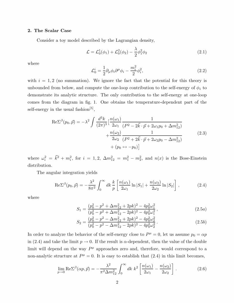
with i = 1, 2 (no summation). We ignore the fact that the potential for this theory is

unbounded from below, and compute the one-loop contribution to the self-energy of φ1 to

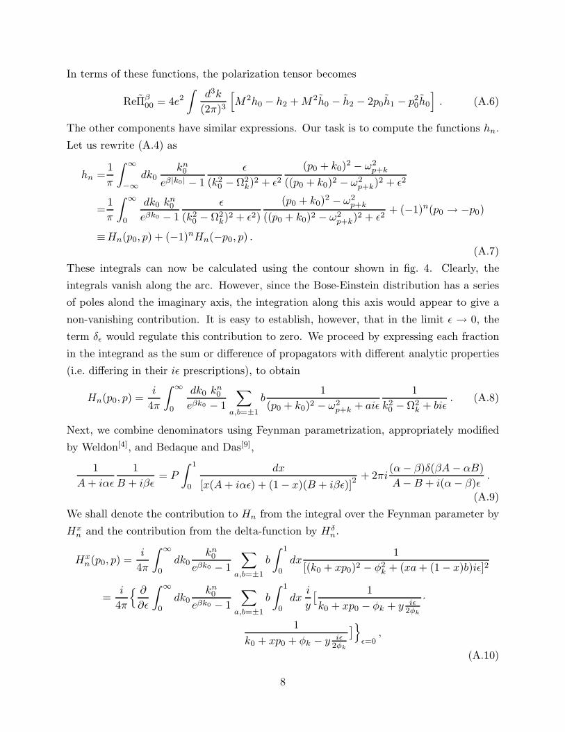
demonstrate its analytic structure. The only contribution to the self-energy at one-loop

comes from the diagram in fig. 1. One obtains the temperature-dependent part of the

self-energy in the usual fashion[5],

ReΣβ(p0, ~p) = −λ2

∫

d3k

(2π)3[n(ω1)

2ω1

1

(P 2 − 2~k · ~p + 2ω1p0 + ∆m212)

+n(ω2)

2ω2

1

(P 2 + 2~k · ~p + 2ω2p0 − ∆m212)

+ (p0 ↔ −p0)]

(2.3)

where ω2i = ~k2 + m2

i , for i = 1, 2, ∆m212 = m2

1 − m22, and n(x) is the Bose-Einstein

distribution.

The angular integration yields

ReΣβ(p0, ~p) = − λ2

8π2

∫ ∞

0

dkk

p

[

n(ω1)

2ω1ln |S1| +

n(ω2)

2ω2ln |S2|

]

, (2.4)

where

S1 =(p2

0 − p2 + ∆m212 + 2pk)2 − 4p2

0ω21

(p20 − p2 + ∆m2

12 − 2pk)2 − 4p20ω

21

, (2.5a)

S2 =(p2

0 − p2 − ∆m212 + 2pk)2 − 4p2

0ω22

(p20 − p2 − ∆m2

12 − 2pk)2 − 4p20ω

22

. (2.5b)

In order to analyze the behavior of the self-energy close to Pµ = 0, let us assume p0 = αp

in (2.4) and take the limit p → 0. If the result is α-dependent, then the value of the double

limit will depend on the way Pµ approaches zero and, therefore, would correspond to a

non-analytic structure at Pµ = 0. It is easy to establish that (2.4) in this limit becomes,

limp→0

ReΣβ(αp, ~p) = − λ2

π2∆m212

∫ ∞

0

dk k2

[

n(ω1)

2ω1− n(ω2)

2ω2

]

. (2.6)

2

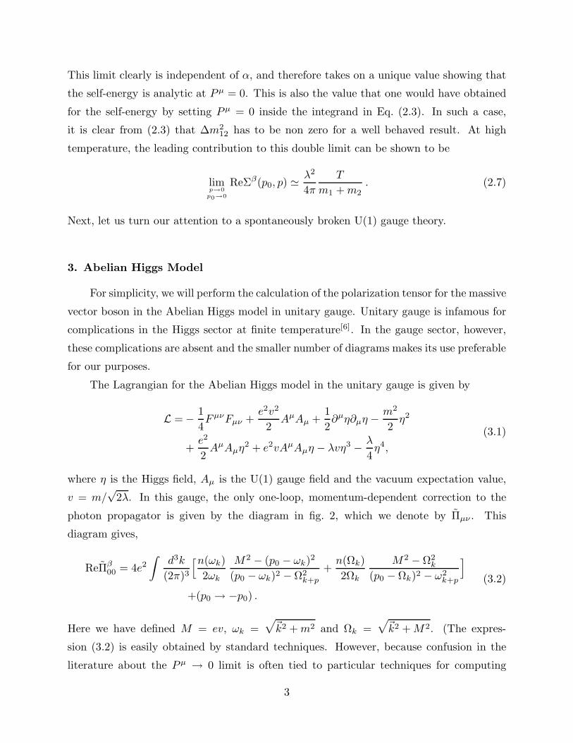
This limit clearly is independent of α, and therefore takes on a unique value showing that

the self-energy is analytic at Pµ = 0. This is also the value that one would have obtained

for the self-energy by setting Pµ = 0 inside the integrand in Eq. (2.3). In such a case,

it is clear from (2.3) that ∆m212 has to be non zero for a well behaved result. At high

temperature, the leading contribution to this double limit can be shown to be

limp→0

p0→0

ReΣβ(p0, p) ≃ λ2

4π

T

m1 + m2. (2.7)

Next, let us turn our attention to a spontaneously broken U(1) gauge theory.

3. Abelian Higgs Model

For simplicity, we will perform the calculation of the polarization tensor for the massive

vector boson in the Abelian Higgs model in unitary gauge. Unitary gauge is infamous for

complications in the Higgs sector at finite temperature[6]. In the gauge sector, however,

these complications are absent and the smaller number of diagrams makes its use preferable

for our purposes.

The Lagrangian for the Abelian Higgs model in the unitary gauge is given by

L = − 1

4FµνFµν +

e2v2

2AµAµ +

1

2∂µη∂µη − m2

2η2

+e2

2AµAµη2 + e2vAµAµη − λvη3 − λ

4η4,

(3.1)

where η is the Higgs field, Aµ is the U(1) gauge field and the vacuum expectation value,

v = m/√

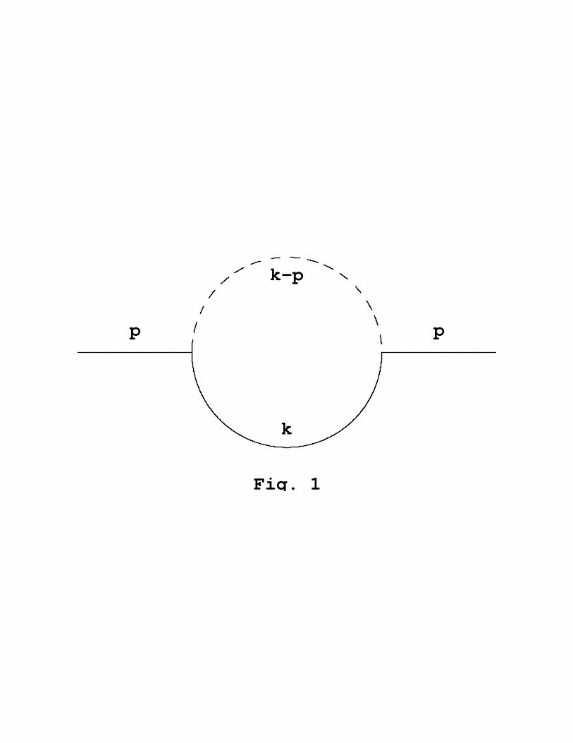
2λ. In this gauge, the only one-loop, momentum-dependent correction to the

photon propagator is given by the diagram in fig. 2, which we denote by Πµν . This

diagram gives,

ReΠβ00 = 4e2

∫

d3k

(2π)3

[n(ωk)

2ωk

M2 − (p0 − ωk)2

(p0 − ωk)2 − Ω2k+p

+n(Ωk)

2Ωk

M2 − Ω2k

(p0 − Ωk)2 − ω2k+p

]

+(p0 → −p0) .

(3.2)

Here we have defined M = ev, ωk =√

~k2 + m2 and Ωk =√

~k2 + M2. (The expres-

sion (3.2) is easily obtained by standard techniques. However, because confusion in the

literature about the Pµ → 0 limit is often tied to particular techniques for computing

3

finite-temperature diagrams, and since the use of Feynman parametrization in the real-

time formalism is a particularly good example of this, we show explicitly in the appendix

how to perform such a calculation using this technique, together with regularization of

the real-time propagators. For routine calculations, however, Feynman parametrization is

impractical.) After doing the angular integration, one obtains

ReΠβ00(p0, p) = − e2

2π2

∫ ∞

0

dk k

[

(∆m212 + k2 + p2

0)n(ωk)

2ωk

1

pln |S1| +

k2n(Ωk)

2Ωk

1

pln |S2|

+ n(ωk)p0

pln

∣

∣

∣

∣

(p20 − p2 + ∆m2

12)2 − 4(p0ωk + pk)2

(p20 − p2 + ∆m2

12)2 − 4(p0ωk − pk)2

∣

∣

∣

∣

]

,

(3.3)

where Si are given in (2.5 ) with m1 = m and m2 = M .

Let us analyze the small-p0, small-p behavior of (3.3). For that purpose, let us set as

before

p0 = αp . (3.4)

Then, for nonzero values of ∆m212 = m2 − M2, it is clear that

limp→0

ReΠβ00(αp, p) = −4e2

π2

∫ ∞

0

dk

[

k2 n(ωk)

2ωk+

k4

m2 − M2

(

n(ωk)

2ωk− n(Ωk)

2Ωk

)]

. (3.5)

In particular, this limit is finite, α-independent and hence independent of the ratio p0/p

as p0 and p approach zero. Alternatively, this may be obtained by simply putting Pµ = 0

in (3.2). So, the double limit is unique, as promised. Furthermore, it is easy to establish

that ReΠβii has a unique double limit as well.

The high-temperature limit of (3.5) can be easily obtained to be

limp→0

p0→0

ReΠβ00(p0, p) =

1

2e2T 2 , (3.6)

which turns out to be the same as the (p0 = 0, ~p → 0) limit of the equal mass case

∆m212 = 0. (In fact, we note here that even though the expression (3.5) appears to be

singular when m = M , it indeed has a finite limit as the two masses become degenerate

and corresponds to the p0 = 0, ~p → 0 limit of the degenerate case. One can, therefore,

even foresee using such a mass-splitting regularization in such calculations for the equal

mass case.)

4

4. Summary and Physical Implications

We have shown, both in the context of a scalar toy model as well as for a spontaneously

broken Abelian gauge theory, that the finite-temperature one-loop self-energy/polarization

tensor at finite temperature has a unique limit as the external four-momentum goes to zero.

The absence of the usual non-commuting double limits is traced to the fact that there is

(generically) a finite mass difference among the particles propagating in the loop. One can

understand this result in the following way. The real part of the one-loop self-energy is

related to the imaginary part through the dispersion relation[4],

ReΣβR(p0, p) =

1

πP

∫ ∞

−∞

duImΣβ

R(u, p)

u − p0

=2

πP

∫ ∞

0

du uImΣβ

R(u, p)

u2 − p20

.

(4.1)

The last equality follows from the fact that ImΣβR(p0, p) is an odd function of p0

[7]. Here

ΣβR is the retarded two point function related to Σβ by

ImΣβR(u, p) = ImΣβ(u, p) tanh

βu

2

ReΣβR(u, p) = ReΣβ(u, p) .

(4.2)

As pointed out by Weldon[3], ImΣβR(u, p) is non-zero only for some values of u2 − p2.

The imaginary part of the self-energy is expressed in terms of the discontinuity of ΣβR(p0, p)

along these cuts on the real axis,

limǫ→0+

(

ΣβR(p0 + iǫ, p) − Σβ

R(p0 − iǫ, p))

= −2iImΣβR(p0, p) , (4.3)

for real p0. For fixed m1 and m2, these cuts exist for

u2 − p2 ≥ (m1 + m2)2 , (4.4a)

u2 − p2 ≤ (m1 − m2)2 . (4.4b)

The first cut is the usual zero-temperature cut corresponding to the decay of the incoming

particle, whereas the second appears only at T 6= 0 and represents absorption of a particle

from the medium. The first cut does not lend itself to non-commuting double limits, so

the only suspect is the second cut. In fact, it is this cut which is responsible for the non-

commuting double limits in the case m1 = m2[4]. In our case however, the contribution

5

of this cut is perfectly well-behaved as Pµ → 0. In fact, if we denote this contribution by

C2(p0, p), then we obtain

ReΣβR(p0, p) ∋ C2(p0, p) =

2

πP

∫ (p2+(m1−m2)2)

12

0

du uImΣβ

R(u, p)

u2 − p20

. (4.5)

Performing the change of variables u → u/√

p2 + (m1 − m2)2, we obtain

ReΣβR(p0, p) ∋ C2(p0, p) =

2

πP

∫ 1

0

du uImΣβ

R(u√

p2 + (m1 − m2)2, p)

u2 − p20

p2+(m1−m2)2

. (4.6)

As long as the masses are different, the zero momentum limit of C2(p0, p) is well-defined

and given by

C2(0, 0) =2

π

∫ |m1−m2|

0

duImΣβ

R(u, 0)

u. (4.7)

This limit, however, is not well-defined if the masses are equal. Note that (4.7) is well-

behaved, given that ImΣβ(u, 0) is odd in u, and goes as u for small u.

The results of the previous section might, at first, appear to have far-reaching conse-

quences in the study of finite-temperature field theory, where it has always been assumed

that all one-loop self-energies exhibit a non-analytic behavior at vanishing external four-

momentum. One may naturally wonder whether our observation has any effect on stan-

dard computations of physical quantities, such as the difference between Debye and plasmon

masses in the standard electroweak theory, and whether there could be any effect on studies

of the electroweak phase transition[8]. In fact it does not, as can be argued in the following

way. Our result (3.6) for the Pµ → 0 limit depends on assuming p0, p ≪ |∆m2|/T in (3.2),

since (3.2) is dominated by k ∼ T . However, the region of interest for self-consistently

finding the Debye or plasmon poles of the vector propagator is when p0 or p take values

of order mi ≫ |∆m2|/T . In that regime, ∆m212 can be ignored in (3.3), in which case one

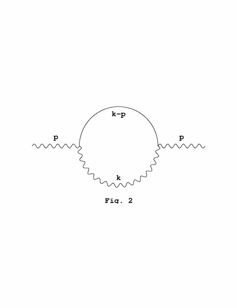
recovers the usual non-commuting double limits. The qualitative features of our results

are shown in fig. 3. For p0 and p small compared to |∆m2|/T , the functions Πβ00(p0, 0)

and Πβ00(0, p) tend to the same limit. However, at order m, the functions take on different

values. As the mass difference goes to zero, it is clear that the unique limit disappears, as

well.

6

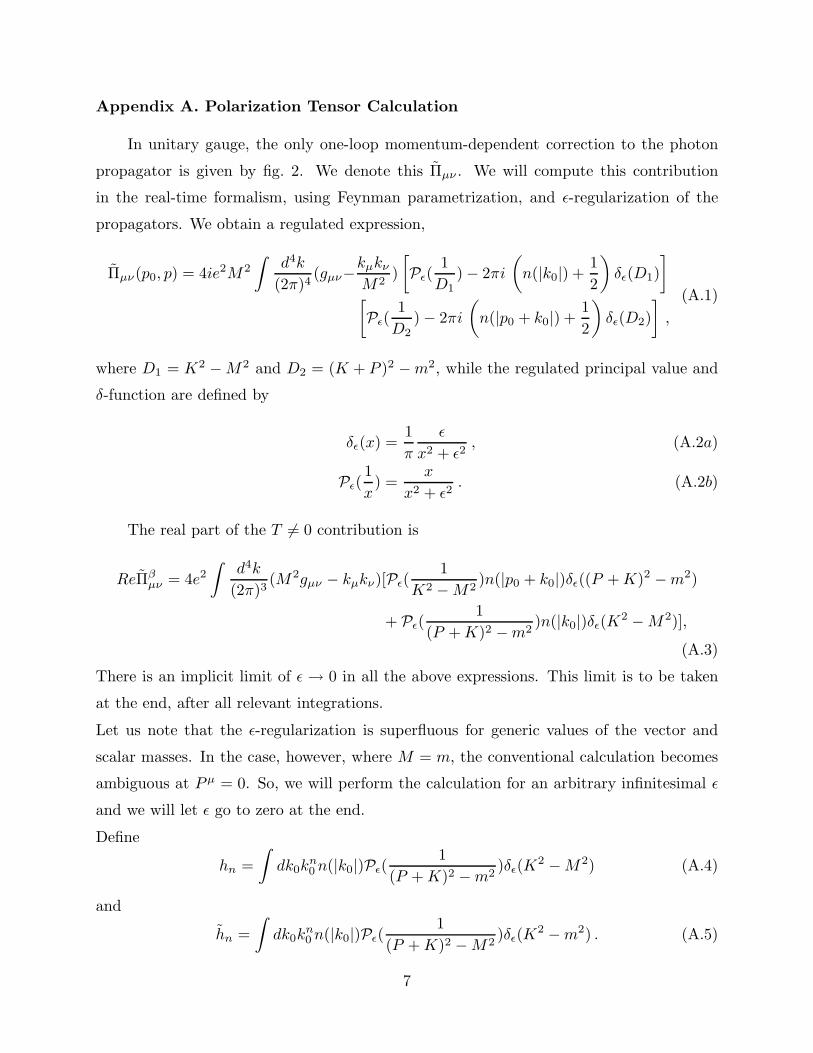
Appendix A. Polarization Tensor Calculation

In unitary gauge, the only one-loop momentum-dependent correction to the photon

propagator is given by fig. 2. We denote this Πµν . We will compute this contribution

in the real-time formalism, using Feynman parametrization, and ǫ-regularization of the

propagators. We obtain a regulated expression,

Πµν(p0, p) = 4ie2M2

∫

d4k

(2π)4(gµν−

kµkν

M2)

[

Pǫ(1

D1) − 2πi

(

n(|k0|) +1

2

)

δǫ(D1)

]

[

Pǫ(1

D2) − 2πi

(

n(|p0 + k0|) +1

2

)

δǫ(D2)

]

,

(A.1)

where D1 = K2 − M2 and D2 = (K + P )2 − m2, while the regulated principal value and

δ-function are defined by

δǫ(x) =1

π

ǫ

x2 + ǫ2, (A.2a)

Pǫ(1

x) =

x

x2 + ǫ2. (A.2b)

The real part of the T 6= 0 contribution is

ReΠβµν = 4e2

∫

d4k

(2π)3(M2gµν − kµkν)[Pǫ(

1

K2 − M2)n(|p0 + k0|)δǫ((P + K)2 − m2)

+ Pǫ(1

(P + K)2 − m2)n(|k0|)δǫ(K

2 − M2)],

(A.3)

There is an implicit limit of ǫ → 0 in all the above expressions. This limit is to be taken

at the end, after all relevant integrations.

Let us note that the ǫ-regularization is superfluous for generic values of the vector and

scalar masses. In the case, however, where M = m, the conventional calculation becomes

ambiguous at Pµ = 0. So, we will perform the calculation for an arbitrary infinitesimal ǫ

and we will let ǫ go to zero at the end.

Define

hn =

∫

dk0kn0 n(|k0|)Pǫ(

1

(P + K)2 − m2)δǫ(K

2 − M2) (A.4)

and

hn =

∫

dk0kn0 n(|k0|)Pǫ(

1

(P + K)2 − M2)δǫ(K

2 − m2) . (A.5)

7

In terms of these functions, the polarization tensor becomes

ReΠβ00 = 4e2

∫

d3k

(2π)3

[

M2h0 − h2 + M2h0 − h2 − 2p0h1 − p20h0

]

. (A.6)

The other components have similar expressions. Our task is to compute the functions hn.

Let us rewrite (A.4) as

hn =1

π

∫ ∞

−∞

dk0kn0

eβ|k0| − 1

ǫ

(k20 − Ω2

k)2 + ǫ2(p0 + k0)

2 − ω2p+k

((p0 + k0)2 − ω2p+k)2 + ǫ2

=1

π

∫ ∞

0

dk0 kn0

eβk0 − 1

ǫ

(k20 − Ω2

k)2 + ǫ2)

(p0 + k0)2 − ω2

p+k

((p0 + k0)2 − ω2p+k)2 + ǫ2

+ (−1)n(p0 → −p0)

≡Hn(p0, p) + (−1)nHn(−p0, p) .

(A.7)

These integrals can now be calculated using the contour shown in fig. 4. Clearly, the

integrals vanish along the arc. However, since the Bose-Einstein distribution has a series

of poles alond the imaginary axis, the integration along this axis would appear to give a

non-vanishing contribution. It is easy to establish, however, that in the limit ǫ → 0, the

term δǫ would regulate this contribution to zero. We proceed by expressing each fraction

in the integrand as the sum or difference of propagators with different analytic properties

(i.e. differing in their iǫ prescriptions), to obtain

Hn(p0, p) =i

4π

∫ ∞

0

dk0 kn0

eβk0 − 1

∑

a,b=±1

b1

(p0 + k0)2 − ω2p+k + aiǫ

1

k20 − Ω2

k + biǫ. (A.8)

Next, we combine denominators using Feynman parametrization, appropriately modified

by Weldon[4], and Bedaque and Das[9],

1

A + iαǫ

1

B + iβǫ= P

∫ 1

0

dx

[x(A + iαǫ) + (1 − x)(B + iβǫ)]2 + 2πi

(α − β)δ(βA − αB)

A − B + i(α − β)ǫ.

(A.9)

We shall denote the contribution to Hn from the integral over the Feynman parameter by

Hxn and the contribution from the delta-function by Hδ

n.

Hxn(p0, p) =

i

4π

∫ ∞

0

dk0kn0

eβk0 − 1

∑

a,b=±1

b

∫ 1

0

dx1

[(k0 + xp0)2 − φ2k + (xa + (1 − x)b)iǫ]2

=i

4π

∂

∂ǫ

∫ ∞

0

dk0kn0

eβk0 − 1

∑

a,b=±1

b

∫ 1

0

dxi

y

[ 1

k0 + xp0 − φk + y iǫ2φk

·

1

k0 + xp0 + φk − y iǫ2φk

]

ǫ=0,

(A.10)

8

where

φk = (−x(1 − x)p20 + (1 − x)Ω2

k + xω2p+k)

12 , (A.11)

and

y = x(a − b) + b . (A.12)

We are now able to do the k0-integration by picking the poles in the first quadrant,

Hxn(p0, p) = − i

2

∂

∂ǫ

[

∫ 1

0

dx1

2φk + iǫφk

(φk − xp0 + iǫ2φk

)n

eβ(φk−xp0+ iǫ

2φk) − 1

+

∫ 12

0

dx

1 − 2x

1

2φk + (1 − 2x) iǫφk

(φk − xp0 + (1 − 2x) iǫ2φk

)n

eβ(φk−xp0+(1−2x) iǫ

2φk) − 1

∫ 1

12

dx

1 − 2x

1

2φk − (1 − 2x) iǫφk

(φk − xp0 − (1 − 2x) iǫ2φk

)n

eβ(φk−xp0−(1−2x) iǫ

2φk) − 1

]

ǫ=0.

(A.13)

Upon defining a new variable

zk(α) = (−x(1 − x)p20 + (1 − x)Ω2

k + xω2p+k + α)

12 , zk(0) = φk (A.14)

Eq. (A.13) reduces to

Hxn(p0, p) =

1

2

∂

∂α

∫ 12

0

dx

zk

(zk − xp0)n

eβ(zk−xp0) − 1

α=0. (A.15)

The term involving the delta-function in the Feynman parametrization formula can be

easily computed to contribute

Hδn(p0, p) = − 1

2R

(−p0/2 + R)n

eβ(−p0/2+R) − 1

1

ω2p+k − Ω2

k − 2p0R, (A.16)

where

R =

√

−p20

4+

1

2(ω2

p+k + Ω2k) . (A.17)

The function hn, defined by (A.5) can be calculated in the same fashion.

Recalling (A.6), and collecting only the Feynman parameter dependent terms, we obtain

ReΠβ00 ∋ 2e2

∂

∂α

∫

d3k

(2π)3

∫ 12

0

dx (M2 − (zk + xp0)2)

n(zk + xp0)

zk

+(M2 − (zk + (1 − x)p0)2)

n(zk − xp0)

zk

α=0

+(p0 → −p0) ,

(A.18)

9

where zk ↔ zk as m ↔ M . The x-integration can be performed after a change of variables

x → 1 − x

~k → −~k − ~p ,(A.19)

in the second term, and

w = zk + xp0 , (A.20)

in the resulting integrand. All the dependence on α resides now in the limits of integration.

Taking the derivative with respect to α and the limit α → 0 yields,

ReΠβ00 ∋ 2e2

∫

d3k

(2π)3

[n(ωk)

ωk

M2 − (p0 − ωk)2

(p0 − ωk)2 − Ω2k+p

+n(Ωk)

Ωk

M2 − Ω2k

(p0 − Ωk)2 − ω2k+p

+1

R

M2 − 12(Ω2

k + ω2p+k) − p0R

ω2p+k − Ω2

k + 2p0R

[ 1

eβ(p02

+R) − 1− 1

eβ(−p02

+R) − 1

]

]

+(p0 → −p0) ,

(A.21)

where R is given by Eq. (A.17). If the delta function contribution to the Feynman

parametrization formula (A.9) were incorrectly left out, then (A.21) would be the complete

expression for ReΠβ00. It is interesting to note that in such a case (A.21) would agree with

the expression derived within the imaginary-time formalism for p0 = 2πiℓT , since then the

third term would vanish identically. However, (A.21) as it stands is the wrong analytic

continuation of the euclidean expression. Indeed, the contribution of the delta function

(A.16) exactly cancels the third term in (A.21) and, therefore, the complete expression is

ReΠβ00 = 4e2

∫

d3k

(2π)3

[n(ωk)

2ωk

M2 − (p0 − ωk)2

(p0 − ωk)2 − Ω2k+p

+n(Ωk)

2Ωk

M2 − Ω2k

(p0 − Ωk)2 − ω2k+p

]

+(p0 → −p0) ,

(A.22)

which agrees with the imaginary-time expression for real p0.

P.A. was supported by DOE grant DE-FG06-91ER40614. P.B. was supported in part

by DOE grant DE-FG02-91ER40685 and in part by CAPES. A.D. was supported in part by

DOE grant DE-FG02-91ER40685. A.D. also thanks the Division of Educational Programs

of Argonne National Laboratory. S.V. was supported by DOE grants DE-FG06-91ER40614

and W-31-109-ENG-38. S.V. acknowledges useful discussions with G. Bodwin, L. Brown,

I. Knowles, L. Yaffe, and C. Zachos and thanks U. Sarid for his Feynman diagram drawing

code.

10

References

[1] V. P. Silin, Sov. Phys. JETP 11, 1136 (1960);

D.J. Gross, R.D. Pisarski and L.G. Yaffe, Rev. Mod. Phys. 53, 43 (1981);

V.V. Klimov, Sov. Phys. JETP 55, 199 (1982);

H.A. Weldon, Phys. Rev. D26, 1394 (1982);

E. Braaten and R. D. Pisarski, Nucl. Phys. B337, 569 (1990) and B339, 310 (1990),

Phys. Rev. Lett. 64, 1338 (1990), Phys. Rev. D45, 1827 (1992);

J. Frenkel and J. C. Taylor, Nucl. Phys. B334, 199 (1990) and B374, 156 (1992).

[2] Y. Fujimoto and H. Yamada, Z. Phys. C37, 265 (1988);

P. S. Gribosky and B. R. Holstein, Z. Phys. C47, 205 (1990);

P. Bedaque and A. Das, Phys. Rev. D45, 2906 (1992)

[3] H. A. Weldon, Phys. Rev. D28, 2007 (1983). Our expression (4.4b) for the T 6= 0 cut

disagrees with Weldon’s corresponding cut.

[4] H. A. Weldon, West Virginia University Preprint WVU-992 (August 1992).

[5] The reader wishing an introduction to perturbation theory at finite temperature may

try J.I. Kapusta, “Finite-temperature field theory” Cambridge Univ. Press, Cam-

bridge, 1989.

[6] P. Arnold, E. Braaten, and S. Vokos, Phys. Rev. D46, 3576 (1992).

[7] A. A. Abrikosov, L. P. Gorkov and I. E. Dzyaloshinski, “Methods of Quantum Field

Theory in Statistical Physics”, Dover, New York, 1963;

A. L. Fetter and J. D. Walecka, “Quantum Theory of Many Particle Systems”,

McGraw-Hill, New York, 1971;

H. Umezawa, H. Matsumoto, and M. Tachiki, “Thermo Field Dynamics and Con-

densed States”, North-Holland, Amsterdam, 1982;

S. Jeon, Univ. of Washington Preprint UW/PT-92-03.

[8] M. Carrington, Phys. Rev. D45, 2933 (1992);

M. Dine, G. Leigh, P. Huet, A. Linde, and D. Linde, Phys. Rev. D46, 550 (1992), and

Phys. Lett. B283, 319 (1992);

G. Boyd, D. Brahm, S. Hsu, Enrico Fermi Institute Preprint EFI-92-22 (1992);

P. Arnold and O. Espinosa, Univ. of Washington Preprint UW/PT-92-18.

[9] P. Bedaque and A. Das, Rochester Preprint UR 1275, ER-40685-727 (September 1992).

11

Figure Captions

Fig. 1. The one-loop contribution to the φ1 self-energy.

Fig. 2. The only one-loop, momentum-dependent contribution to the vector self-energy,

in unitary gauge.

Fig. 3. For p0 and p small compared to |∆m2|/T , the functions Πβ00(p0, 0) and Πβ

00(0, p)

tend to the same limit. However, at order m, the functions take on different

values. As the mass difference goes to zero, it is clear that the unique limit

disappears, as well.

Fig. 4. Contour in the complex k0-plane used in the integration. The limit ǫ′ → 0 is

implied.

12

p p

k-p

k

Fig. 1

p p

k-p

k

Fig. 2

Fig. 3

Π00(0,p)

Π00(p ,0)0

(p ,p)0~m~∆m2/T

(eT)2

3

_

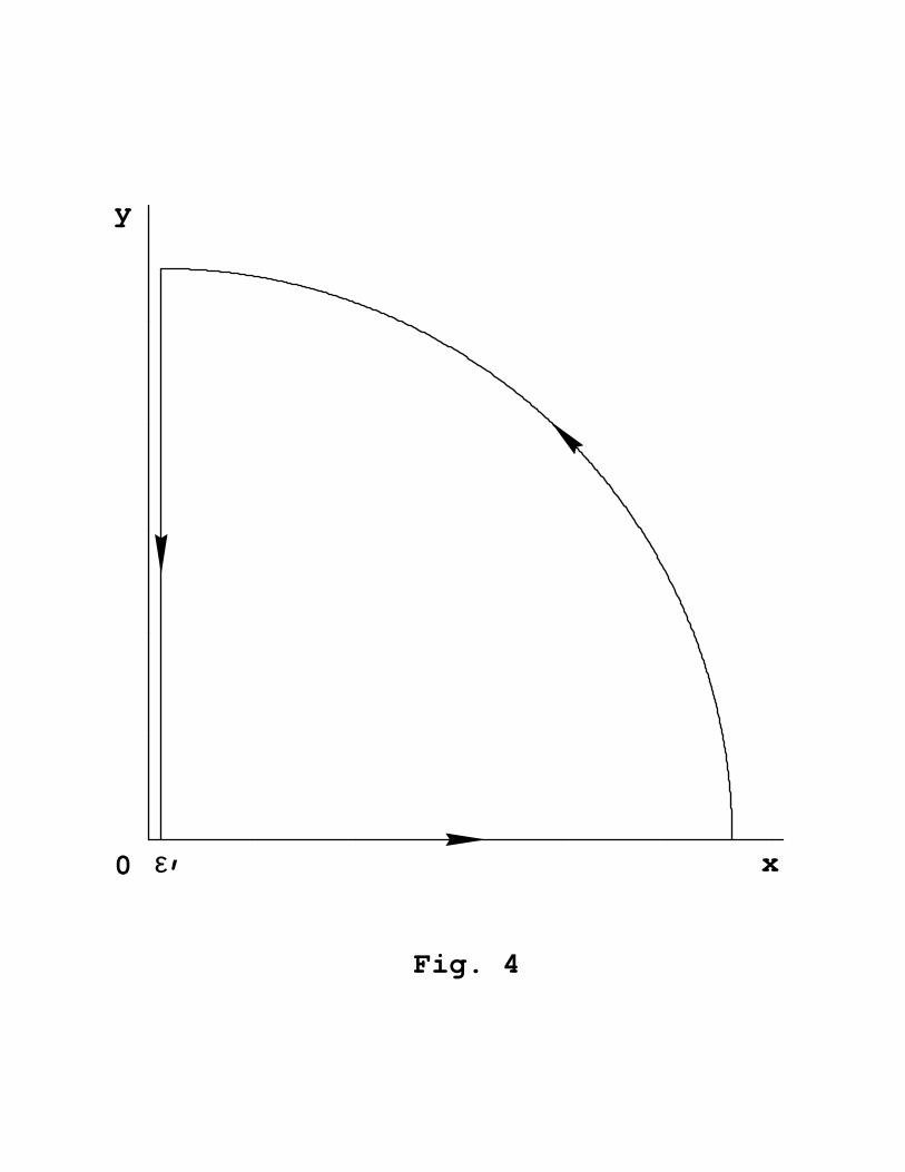
Fig. 4

x

y

0 ε’