Analysis of unsteady reacting flows and impact of chemistry description in Large Eddy Simulations of...

Combustion and Flame 157 (2010) 176–191

Contents lists available at ScienceDirect

Combustion and Flame

journal homepage: www.elsevier .com/locate /combustflame

Analysis of unsteady reacting flows and impact of chemistry descriptionin Large Eddy Simulations of side-dump ramjet combustors

A. Roux a, L.Y.M. Gicquel a,*, S. Reichstadt b, N. Bertier b, G. Staffelbach a, F. Vuillot b, T.J. Poinsot c

a CERFACS, 42 Av. G. Coriolis, 31057 Toulouse Cedex, Franceb ONERA, BP 72, 29 Avenue de la Division Leclerc, 92322 Châtillon Cedex, Francec IMFT, Avenue C. Soula, 31400 Toulouse, France

a r t i c l e i n f o a b s t r a c t

Article history:Received 1 April 2009Received in revised form 31 July 2009Accepted 30 September 2009Available online 31 October 2009

Keywords:Large Eddy SimulationCombustionAcousticRamjetChemical scheme

0010-2180/$ - see front matter � 2009 The Combustdoi:10.1016/j.combustflame.2009.09.020

* Corresponding author. Fax: +33 5 61 19 30 00.E-mail address: [email protected] (L.Y.M. Gicquel

Among all the undesired phenomena observed in ramjet combustors, combustion instabilities are offoremost importance and predicting them using Large Eddy Simulation (LES) is an active research field.While acoustics are naturally captured by compressible LES provided that the proper boundary condi-tions are applied, combustion/chemistry modelling remains a critical issue and its impact on numericalpredictions must still be assessed for complex applications. To do so, two different ramjet LES’s are com-pared here. The first simulation is based on a standard one-step chemistry known to over-estimate thelaminar flame speed in fuel rich conditions. The second simulation uses the same scheme but introducesa correction of reaction rates for rich flames to match a detailed mechanism provided by Peters (1993)[1]. Even though the two chemical schemes are very similar and very few points burn in rich regimes,distinct limit-cycles are obtained with LES depending on which scheme is used. Results obtained withthe standard one-step chemistry exhibit high frequency self-sustained oscillations. Multiple flame frontsare stabilized in the vicinity of the shear layer developing at the exit of the air inlets. When compared tothe experiment, the fitted one-step scheme yields better predictions than the standard scheme. With thefitted scheme, the flame is detached from the air inlets and stabilizes in the regions identified in theexperiment (Ristori et al. (2005) [2], Heid and Ristori (2003) [3], Heid and Ristori (2005) [4], Ristoriet al. (1999) [5]). LES and experiments exhibit all main low-frequency modes including the first longitu-dinal acoustic mode. The high frequencies excited with the standard scheme are damped with the fittedscheme. The chemical scheme is found, for this ramjet burner, to have a strong impact on the predictedstability: approximate chemical schemes even in a limited range of equivalence ratio can lead to theoccurence of non-physical combustion oscillations.

� 2009 The Combustion Institute. Published by Elsevier Inc. All rights reserved.

1. Introduction

Large Eddy Simulation (LES) is a very successful tool to describeturbulence and its interactions with other physical phenomenasuch as mixing or combustion in experimental or industrial config-urations [6–8]. LES solves the filtered Navier–Stokes equations(NSE) to describe the larger scales of turbulent flows while smallerscale effects are modelled. It has become standard to study turbu-lent reacting flows in modern combustion devices such as aeronau-tical gas turbines or rocket engines [9–14].

Recent numerical predictions obtained by LES for turbulent react-ing flows [15–18] underline the power of the approach for laboratoryand industry like configurations. Most recent LES’s have focused ongas turbine configurations because these systems exhibit a varietyof difficult problems that are well addressed through that fully

ion Institute. Published by Elsevier

).

unsteady approach: ignition, quenching, thermo-acoustic instabili-ties. . . Ramjets have received less attention since the pioneeringwork of Kailasanath [19]. Only a few studies have been devoted spe-cifically to LES of ramjets [19–23]. This type of combustor exhibitssignificant differences compared to gas turbine flows: the velocitiesare much higher, combustion is not stabilized by swirl, a chokednozzle terminates the chamber. Low-frequency instabilities are alsopresent and must be avoided to prevent extinction or even destruc-tion of the configuration. Most importantly, chemistry may play adetermining role due to the absence of flame holder in the combus-tion chamber.

Although the speed of computers continuously increases, somechoices have to be made in order to spare computational cost to han-dle real applications and their inherent complexities. For reactingflows, using directly complex chemical schemes is prohibited be-cause of the numerous reactions and reactants which induce largecomputing efforts. Moreover, these chemical schemes are often verystiff and require accurate and expensive solvers. New methodologies

Inc. All rights reserved.

http://dx.doi.org/10.1016/j.combustflame.2009.09.020

mailto:[email protected]

http://www.sciencedirect.com/science/journal/00102180

http://www.elsevier.com/locate/combustflame

A. Roux et al. / Combustion and Flame 157 (2010) 176–191 177

allow to reduce the cost of complex chemical schemes by projectiononto a reduced set of coordinates, typically a progress variable and amixture fraction, (Intrinsic Low-Dimensional Manifold – ILDM –,Flame-Prolongation of ILDM – FPI – or Flamelet-Generated Manifold– FGM – [24–30], In-Situ Adaptive Tabulation – ISAT – [31]). Suchtabulation methods require large amounts of memory space and thiscan affect parallelization of the code even if potential improvementson that specific point are currently being studied [32]. As of today,many reactive LES’s are thus limited to using simple chemicalschemes [8–14] and the impact of such simple schemes on the reli-ability of LES predictions is still an open issue. In a first attempt to ad-dress this issue, we limit our study to the context of thermo-acousticinstabilities in ramjet burners. For such a problem, only heat releaserate and acoustics are believed to determine the operating limit-cy-cle, gas composition having a limited impact which justifies the useof simple chemical schemes.

We present here the application of LES to a side-dump ramjetfor wich experimental data provided by the French AerospaceLab. (ONERA) is available for different non-reacting and reactingconditions [2]. The device burns gaseous propane fed through thehead-end by two jets (global equivalence ratio of 0.75). Contrarilyto previous computations on the same burner [21,33], the compu-tational domain treats the entire combustion chamber: the pro-pane injection, the choked air intakes with square cross sectionsand a choked nozzle prior to the exit. Note that the configurationis acoustically closed which allows to compare the differentfrequencies, found in the experiment and the LES, in a rigorousmanner. Two single-step chemical mechanisms will be used inthe LES and the impact of these schemes on the mean and unsteadystructure of the flame will be studied.

2. Experimental facility

In 1995, ONERA launched a specific program named ‘‘ResearchRamjet Program” to understand the different processes appearingin such a configuration [2–5,22]. In this side-dump ramjet combus-tor, Particle Doppler Anemometer (PDA), Laser Doppler Velocimetry(LDV) and Particle Imagery Velocity (PIV) measurements were per-formed to provide mean and oscillating velocities. A first set ofexperiments allows to investigate the non-reacting flow and themixing by studying the influence of equivalence ratio on fuel pene-tration. Reacting flow conditions are studied thanks to Particle LaserInduced Fluorescence (PLIF) based on OH or CH emissions. A high-speed camera (up to 2,000 Hz) gives a view of the flame whereasmicrophones characterize oscillations within the configuration. Sev-eral flight conditions are evaluated: inlet temperature and mass flowrate change from 520 K, 2.9 kg/s to 750 K, 0.9 kg/s. A range of equiv-alence ratio / from 0.35 to 1.0 has been investigated.

Fig. 1. Sketch of the ONERA

The burner is composed of two air inlets beginning with chokednozzles, Fig. 1. They feed the main combustion chamber through100� 100 mm2 rectangular ducts. Fuel, gaseous propane, is in-jected by eight holes at 350 K into a pre-injection chamber. Thisbox then feeds the head-end region through two 11 mm diametercircular tubes. The combustion chamber is 1261 mm in length andopens onto a choked nozzle which has a throat section of55:8� 100 mm2.

3. Numerical approach

3.1. Governing equations and LES models

LES of reacting flows involves the spatial Favre filtering opera-tion that reduces for spatially, temporally invariant and localisedfilter functions [34] to:

gfðx; tÞ ¼ 1qðx; tÞ

Z þ1

�1qðx0; tÞf ðx0; tÞGðx0 � xÞdx0; ð1Þ

where G denotes the filter function.In the mathematical description of compressible turbulent

flows with chemical reactions and species transport, the primaryvariables are the species volumic mass fractions qaðx; tÞ, the veloc-ity vector uiðx; tÞ, the total energy etðx; tÞ � es þ 1=2uiui and thedensity qðx; tÞ ¼

PNa¼1qaðx; tÞ.

The multispecies fluid follows the ideal gas law, p ¼ qrT andes ¼

R T0 CpdT � p=q, where es is the mixture sensible energy, T the

temperature, Cp the fluid heat capacity at constant pressure and ris the mixture gas constant. The LES solver takes into accountchanges of heat capacity with temperature and composition usingtabulated values of individual species heat capacities. The viscousstress tensor, the heat diffusion vector and the species moleculartransport use classical gradient approaches. The fluid viscosity fol-lows Sutherland’s law, the heat diffusion coefficient follows Fou-rier’s law, and the species diffusion coefficients are obtainedusing a species Schmidt number along with the Hirschfelder Curtisapproximation [6] and velocity corrections for mass conservation.The application of the filtering operation to the instantaneous setof compressible Navier–Stokes transport equations with chemicalreactions yields the LES transport equations [6] which containso-called Sub-Grid Scale (SGS) quantities that need modelling[35,36]. The unresolved SGS stress tensor sij

t , is modelled usingthe Boussinesq assumption [37–39]:

sijt � 1

3skk

tdij ¼ �2qmteSij; with eSij ¼

12

@eui

@xjþ @

euj

@xi

� �� 1

3@euk

@xkdij:

ð2Þ

’s ‘‘Research Ramjet”.

178 A. Roux et al. / Combustion and Flame 157 (2010) 176–191

In Eq. (2), eSij is the resolved strain rate tensor and mt is the SGS tur-bulent viscosity. The Wall Adapting Linear Eddy (WALE) model [40]is chosen to model the SGS viscosity:

mt ¼ðCwDÞ2ðsd

ijsdijÞ

3=2

ðeSijeSijÞ5=2þðsd

ijsdijÞ

5=4; with sd

ij¼12fgij

2þfgji2� �þ1

3fgkk

2dij

ð3ÞIn Eq. (3), D denotes the filter characteristic length (approximatedby the cubic-root of the cell volume), Cw is a model constant equalto 0.49 and fgij is the resolved velocity gradient.

The SGS species flux Jait is modelled using a species SGS turbu-

lent diffusivity Dat ¼ mt=Sca

t , where Scat is the turbulent Schmidt

number (Scat ¼ 0:7 for all a). The SGS energy flux, �qt

i , uses a heatconductivity that is obtained from mt by kt ¼ �qmtCp=Prt , where Prt

is a constant turbulent Prandtl number:

Jait ¼ ��qDa

tWa

W@eXa

@xiþ �qfYaVc

i and qit ¼ �kt

@eT@xiþXN

a¼1

Jati eha

s : ð4Þ

In Eq. (4), the mixture molecular weight W and the species molec-ular weight Wa can be combined with the species mass fraction toyield the expression for the molar fraction of speciesa : Xa ¼ YaW=Wa. Vc

i is the diffusion correction velocity resultingfrom the Hirschfelder Curtis approximation [6] and eT is the Favrefiltered temperature which satisfies the modified filtered stateequation �p ¼ �qreT [41–44]. Finally, ~ha

s stands for the enthalpy of spe-cies a. Note that such expressions introduce higher order terms thatshould require closure in the context of LES. These terms are how-ever usually neglected due to the error introduced by the SGS tur-bulent viscosity hypothesis. Furthermore and although theperformances of the LES closures could be improved through theuse of a dynamic formulation [41,45–48] they are considered suffi-cient to address the present flow configuration.

3.2. Combustion modelling

SGS combustion terms are modelled using the Dynamic Thick-ened Flame (DTF) model [49]. Following the theory of laminar pre-mixed flames [50], the flame speed S0

L and the flame thickness d0L

may be expressed as:

S0L /

ffiffiffiffiffiffikAp

and d0L /

k

S0L

¼ffiffiffikA

r; ð5Þ

where k is the thermal diffusivity and A the pre-exponential con-stant. Increasing the thermal diffusivity by a factor F, the flamespeed is kept unchanged if the pre-exponential factor is decreasedby the same factor [51]. This operation leads to a flame thicknesswhich is multiplied by F and easily resolved on a coarser mesh.Additional information needs however to be supplied so as to prop-erly reproduce the effect of the subgrid-scale interaction betweenturbulence and chemistry [52–54]. This is the intent of the so-calledefficiency function E [55]. When thickening is applied everywherein the flow, the model is limited to fully premixed combustion. Tocompute partially premixed or non-premixed flames [6], a modifiedversion of the Thickened Flame model (DTF) is used here [54,56,57].

With the DTF model, the SGS fluxes are modified to become:

Jait ¼ �ð1� SÞ�qDa

tWa

W@eXa

@xiþ �qfYaVc

i and

qit ¼ �ð1� SÞkt

@eT@xiþXN

a¼1

Jaiteha

s ð6Þ

where S is a sensor detecting reaction zones. The local thickeningfactor depends on the local mesh size: typically thickening must en-sure that enough points are present within the flame zone and thethickening factor F is given by:

F ¼ 1þ ðFmax � 1ÞS and Fmax ¼Nc

Dxd0

L ; ð7Þ

where Nc is the number of points used to resolve the flame front(typically Nc ¼ 5—10).

Although this approach is still being developed and further val-idations are needed, its ease of implementation and it success inprior applications [56–58] assert its suitability for the problem ad-dressed in this work. Aside from these observations, such a modelretains valuable properties which make it suitable for complexapplications:

� when used along with Arrhenius type chemical schemes, finiterate chemical effects are retained (ignition, extinction. . .),

� the balance between chemistry and diffusive effects is preservedwithin the limit of validity of the efficiency function,

� as such it will produce premixed, partially premixed and diffu-sion flames, the former still needing in-depth validation in thecontext of turbulent diffusion flames.

3.3. Numerical schemes

The parallel LES code [59–61] solves the full compressible Na-vier–Stokes equations using a cell-vertex approximation. Thenumerical integration uses Taylor–Galerkin weighted residual cen-tral distribution schemes. This explicit scheme, which providesthird-order accuracy on hybrid meshes, is particularly adequatefor low-dissipation requirements of LES applications [55].

Since the ramjet flow contains choked nozzles, specific shockcapturing techniques are needed for a centered numerical LESscheme to preserve the positivity of the solution in regions wherestrong gradients exist. There, the methodology of Cook and Cabot[62] is used to thicken the shock front by introducing a hypervis-cosity b in the viscous stress tensor sij equivalent to an additionalpressure term,

sijmodified ¼ b� 2

3l

� �@euk

@xkþ 2leSij ð8Þ

where l is the dynamic viscosity and eSij is the symmetric strain ratetensor. The bulk viscosity, b, is modelled as,

b ¼ CðDxÞ4r2keSk and keSk ¼ ðeSijeSjiÞ1=2

; ð9Þ

where C is fixed to 5 according to [62]. This viscosity acts on verysharp velocity gradients characterizing shocks but goes back to zerowhere the velocity evolves smoothly.

3.4. Chemistry model

Two simplified one-step chemical schemes are tested. Theyboth take into account five species (C3H8; O2; CO2; H2O and N2)and are described by the global one-step irreversible reaction,

C3H8 þ 5O2 ! 3CO2 þ 4H2O: ð10Þ

The reaction rate for this reaction reads,

q ¼ AqYC3H8

WC3H8

� �0:856 qYO2

WO2

� �0:503

exp � Ea

RT

� �; ð11Þ

with a pre-exponential factor A ¼ 3:2916� 1010 [cgs] and an activa-tion energy Ea ¼ 31:126 cal mol�1. The exponents used in Eq. (11)are fitted to get the right laminar flame speed in lean conditions.This first scheme will be called in the following ‘‘standard one-stepscheme”.

Fig. 2 shows the comparison between the detailed chemistry gi-ven by Peters [1] and the standard one-step scheme for a givenrange of equivalence ratio. The latter over-estimates flame speeds

Fig. 2. Laminar flame speed and adiabatic flame temperature for the one-step chemical schemes used in LES.

Table 1Boundary Conditions as used in the LES simulations.

Name Boundary type Imposed quantities

Air inlet Non-reflecting inlet _Qair ¼ 0:9 kg s�1, Ti = 750 KFuel inlet Non-reflecting inlet _QC3 H8 ¼ 0:044 kg s�1, Ti = 350 KOutlet Supersonic inlet –Nozzle’s walls Slip adiabatic –Other walls No-slip adiabatic –


for large values of the equivalence ratio (Fig. 2). To circumvent thiswell-known and improper behaviour of single-step schemes, amodified simplified scheme (named ‘‘fitted one-step scheme”) isintroduced.

For this fitted one-step scheme, the pre-exponential A may beadjusted to yield laminar flame speeds over an extended range ofequivalence ratio /. Indeed, laminar flame speed is proportionalto the square root of A. It is thus possible to alter the behaviourof the burning velocity by imposing a functional dependency of Aon the equivalence ratio. Note that such a reasoning infers thatdynamics is to be privileged and that flame positioning is governedby a competition between chemistry and local flow speed. Eq. (11)is thus rewritten as,

q ¼ f ð/ÞA qYC3H8

WC3H8

� �0:856 qYO2

WO2

� �0:503

exp � Ea

RT

� �; ð12Þ

where

f ð/Þ ¼ 12

1þ tanh0:8� /

1:5

� ��

þ 2:114

1þ tanh/� 0:11

0:2

� �� 1þ tanh

1:355� /0:24

� �� :

ð13Þ

Note that adiabatic flame temperatures are not modified by f ð/Þand are still over-estimated with an error of 7% at / ¼ 1. Use of adetailed scheme (if possible in this context) would be the ultimatealternative since not only would the laminar flame speed be correctfor rich conditions but also would be the adiabatic flame tempera-ture. In the specific context of thermo-acoustics, a burner acousticeigenmode shape is determined by the respective location of thecold and hot regions within the burner. Such first order quantitiesare determined by the equilibrium between flow speed and chem-istry, i.e. dynamics. Temperature is of course of importance but witha major impact on the acoustic eigenmode frequency. Finally, notethat for the standard one-step scheme, Schmidt numbers are con-stant but differ from one species to another while the fitted one-step scheme uses equal Schmidt numbers for all species to evaluatethe local mixture fraction and the local equivalence ratio / requiredin Eq. (13) [63].

4. Operating point and boundary conditions

The computed case imposes an air mass flow rate of 0.9 kg/sand a stagnation temperature of 750 K. The associated Reynoldsnumber, based on the inlet duct conditions, is Re ¼ 3:3� 105 andthe global equivalence ratio / ¼ 0:75.

The computational domain contains about 5� 106 tetrahedra(around 9� 105 nodes). The two air inlets are 1 m long with a

square section of 50 mm2 and the main chamber is 1.261 m longwith a square section of 100 mm2.

Choked nozzles and the head-end of the chamber have been lo-cally refined to ensure good resolution of sharp gradients andflame front, in accordance with the requirements for true LES[38]. The minimum grid size is D ¼ 1 mm. The acoustic CFL numberis 0.7 yielding a corresponding time step of about Dt ¼ 3� 10�7 s.As both inlets and outlet are choked (Table 1), all uncertainties onthe acoustic behaviour of the configuration are avoided. Nozzlewalls are handled as slip walls whereas adiabatic laws of the wallare applied on all other walls. Typical yþ values for zones of inter-est stand between 50 and 100. Note that the adiabatic wall hypoth-esis can be discussed since water cooling is applied during theexperiment. The maximum gas temperature is about 2400 K inthe combustion chamber while walls are cooled with water at300 K. Wall heat fluxes could have been imposed to mimic thisphenomenon. However, preliminary evaluations of the impact ofthe adiabatic wall condition compared to fixed temperature wallsdid not show significant impact on the two LES limit-cycles. Since,our primary goal is here to investigate the influence of the kineticscheme on LES predictions, the second set of predictions is not de-tailed in the following.

5. Results

LES results obtained from the simulations with the standardone-step scheme and the fitted one-step scheme are first studiedto extract the main flow features (Reynolds average quantities).The mean flow predictions are then gauged against experimentby comparing mean velocity components in the median planeðZ ¼ 0 mmÞ. Subsection 5.3 presents the instantaneous flow behav-iour and focuses on the combustion processes obtained with thetwo chemical schemes. Limit-cycles are compared based on themain oscillating modes with special attention devoted to the factthat the simulation based on the standard one-step scheme exhib-its high frequencies that are damped in the fitted one-step simula-tion. The final section analyses the reasons leading to thedifferences between the two chemical schemes.

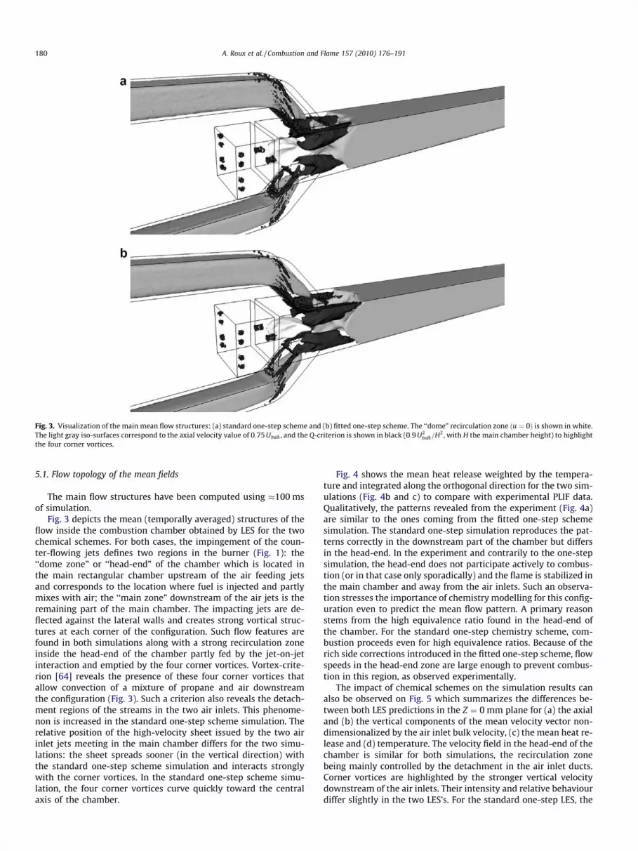
Fig. 3. Visualization of the main mean flow structures: (a) standard one-step scheme and (b) fitted one-step scheme. The ‘‘dome” recirculation zone ðu ¼ 0Þ is shown in white.The light gray iso-surfaces correspond to the axial velocity value of 0:75 Ubulk , and the Q-criterion is shown in black (0:9 U2

bulk=H2, with H the main chamber height) to highlightthe four corner vortices.


5.1. Flow topology of the mean fields

The main flow structures have been computed using �100 msof simulation.

Fig. 3 depicts the mean (temporally averaged) structures of theflow inside the combustion chamber obtained by LES for the twochemical schemes. For both cases, the impingement of the coun-ter-flowing jets defines two regions in the burner (Fig. 1): the‘‘dome zone” or ‘‘head-end” of the chamber which is located inthe main rectangular chamber upstream of the air feeding jetsand corresponds to the location where fuel is injected and partlymixes with air; the ‘‘main zone” downstream of the air jets is theremaining part of the main chamber. The impacting jets are de-flected against the lateral walls and creates strong vortical struc-tures at each corner of the configuration. Such flow features arefound in both simulations along with a strong recirculation zoneinside the head-end of the chamber partly fed by the jet-on-jetinteraction and emptied by the four corner vortices. Vortex-crite-rion [64] reveals the presence of these four corner vortices thatallow convection of a mixture of propane and air downstreamthe configuration (Fig. 3). Such a criterion also reveals the detach-ment regions of the streams in the two air inlets. This phenome-non is increased in the standard one-step scheme simulation. Therelative position of the high-velocity sheet issued by the two airinlet jets meeting in the main chamber differs for the two simu-lations: the sheet spreads sooner (in the vertical direction) withthe standard one-step scheme simulation and interacts stronglywith the corner vortices. In the standard one-step scheme simu-lation, the four corner vortices curve quickly toward the centralaxis of the chamber.

Fig. 4 shows the mean heat release weighted by the tempera-ture and integrated along the orthogonal direction for the two sim-ulations (Fig. 4b and c) to compare with experimental PLIF data.Qualitatively, the patterns revealed from the experiment (Fig. 4a)are similar to the ones coming from the fitted one-step schemesimulation. The standard one-step simulation reproduces the pat-terns correctly in the downstream part of the chamber but differsin the head-end. In the experiment and contrarily to the one-stepsimulation, the head-end does not participate actively to combus-tion (or in that case only sporadically) and the flame is stabilized inthe main chamber and away from the air inlets. Such an observa-tion stresses the importance of chemistry modelling for this config-uration even to predict the mean flow pattern. A primary reasonstems from the high equivalence ratio found in the head-end ofthe chamber. For the standard one-step chemistry scheme, com-bustion proceeds even for high equivalence ratios. Because of therich side corrections introduced in the fitted one-step scheme, flowspeeds in the head-end zone are large enough to prevent combus-tion in this region, as observed experimentally.

The impact of chemical schemes on the simulation results canalso be observed on Fig. 5 which summarizes the differences be-tween both LES predictions in the Z ¼ 0 mm plane for (a) the axialand (b) the vertical components of the mean velocity vector non-dimensionalized by the air inlet bulk velocity, (c) the mean heat re-lease and (d) temperature. The velocity field in the head-end of thechamber is similar for both simulations, the recirculation zonebeing mainly controlled by the detachment in the air inlet ducts.Corner vortices are highlighted by the stronger vertical velocitydownstream of the air inlets. Their intensity and relative behaviourdiffer slightly in the two LES’s. For the standard one-step LES, the

Fig. 4. Integration of heat release weighted by temperature along the orthogonal direction: (a) experimental view, (b) standard one-step scheme and (c) fitted one-stepscheme. Arbitrary levels (from black to white).

Fig. 5. Mean flow quantities in the Z ¼ 0 mm plane. For each sub-figure, top: fitted one-step scheme and bottom: standard one-step scheme. (a) Mean axial velocity. (b) Meanvertical velocity. (c) Mean rate of heat release and d) mean temperature field.


corner vortices’ intensity is larger than in the second LES using thefitted one-step scheme and vortices curve inward the combustionchamber (see also Fig. 3). More noticeable differences between thetwo predictions are observed for quantities directly linked to com-bustion. Heat release fields illustrate the different positions of thereacting fronts. For the standard one-step scheme (Fig. 5c, bottompart), the first front is localized in the vicinity of the shear layer in-duced by the two air inlets near the top and bottom combustorwalls and a second reacting front anchors to the recirculation zonein the head-end. A third and final front may be identified at the on-set of the corner vortices (not visualized here). Such flames are not

identified with the fitted one-step scheme. With this chemicalmodel a unique mean reacting zone is found downstream of theair jet inlets and away from the jet shear layers (Fig. 5c, top part).

Comparisons of LES and experimental velocity fields measuredby ONERA (PIV) at different locations within the combustor andalong different directions are displayed on Fig. 6. Fig. 7 displaysthe axial evolution of the mean axial component of the velocityvector along the symmetry axis of the chamber. In the head-endof the chamber ðX < 180 mmÞ, the two LES’s give similar resultsexcept for the minimum value of the axial velocity which is smallerfor the standard one-step scheme. Note also that the extent of the

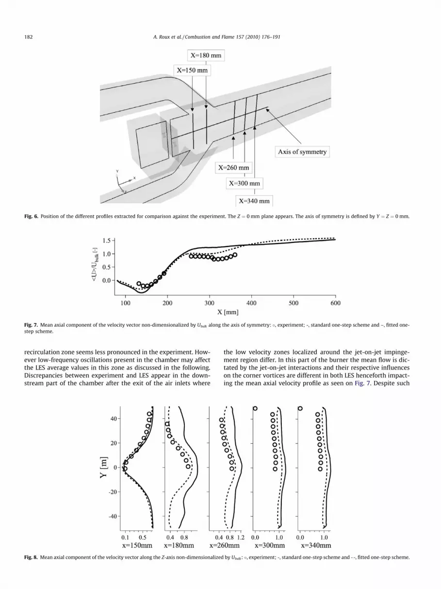
Fig. 6. Position of the different profiles extracted for comparison against the experiment. The Z ¼ 0 mm plane appears. The axis of symmetry is defined by Y ¼ Z ¼ 0 mm.

Fig. 7. Mean axial component of the velocity vector non-dimensionalized by Ubulk along the axis of symmetry: �, experiment; -, standard one-step scheme and –, fitted one-step scheme.


recirculation zone seems less pronounced in the experiment. How-ever low-frequency oscillations present in the chamber may affectthe LES average values in this zone as discussed in the following.Discrepancies between experiment and LES appear in the down-stream part of the chamber after the exit of the air inlets where

Fig. 8. Mean axial component of the velocity vector along the Z-axis non-dimensionalized

the low velocity zones localized around the jet-on-jet impinge-ment region differ. In this part of the burner the mean flow is dic-tated by the jet-on-jet interactions and their respective influenceson the corner vortices are different in both LES henceforth impact-ing the mean axial velocity profile as seen on Fig. 7. Despite such

by Ubulk: �, experiment; -, standard one-step scheme and --, fitted one-step scheme.

Fig. 9. Mean vertical component of the velocity vector along the Z-axis non-dimensionalized by Ubulk: �, experiment; -, standard one-step scheme and --, fitted one-stepscheme.


downstream differences, the position of the stagnation point iswell-predicted by both LES. Finally, both experimental trends andslopes downstream of the chamber ð240 < X < 370 mmÞ are ingood agreement with the fitted one-step scheme simulation. Forthe standard one-step scheme results, the axial velocity reachesits maximum at the end of the air inlet and is delayed furtherdownstream in the fitted one-step scheme simulation. Figs. 8 and9 compare mean experimental results at different axial positions(X = 150 mm, X = 180 mm, X = 260 mm, X ¼ 300 mm and X ¼340 mm) along the Z-axis: i.e. one cut in the head-end of the cham-ber, one at the beginning and at the end of the opening of the airinlets and the last two downstream of the main chamber duct.Overall, LES predictions are in good agreement with the experi-mental data in the head-end of the chamber. Downstream of theair inlet, LES profiles agree with measurements even if the levelsof the axial velocity component with the standard one-step schemesimulation are over-estimated.

Similar comparisons for fluctuating quantities are shown on Figs.10 and 11. Trends are well captured by both simulations and goodagreement is found when comparing experimental data and the

Fig. 10. Standard deviation of axial component of the velocity vector along the Z-axis nonone-step scheme.

standard one-step scheme. Differences with the fitted one-stepscheme are observed but can be partly explained by a potential lackof convergence of these statistics inferred by a different energy con-tent. Indeed, with this scheme the LES flame undergoes a low-fre-quency flapping motion with large variations in the flame positionupstream and downstream of the air inlets as detailed below.

If velocity profiles in the head-end of the combustor are similarfor both simulations, temperature fields strongly differ as shownby Fig. 5. Fig. 12 clearly quantifies the difference by providing theevolution of the mean temperature along the symmetry axis of thecombustor. The two simulations differ in the head-end of the com-bustor where a strong increase of temperature is detected with theone-step scheme simulation. Downstream the air inlets, profilesare similar unlike the axial component of the velocity vector thatshows a first offset with the fitted one-step scheme simulation.

5.2. Unsteady activity

Since the flame positions predicted by the two LES are different,the thermo-acoustic coupling mechanisms can also differ and are

-dimensionalized by Ubulk: �, experiment; -, standard one-step scheme and --, fitted

Fig. 11. Standard deviation of vertical component of the velocity vector along the Z-axis non-dimensionalized by Ubulk: �, experiment; -, standard one-step scheme and --,fitted one-step scheme.

Fig. 12. Mean temperature along the axis of symmetry: -, standard one-step scheme and --, fitted one-step scheme.


investigated here. Four main frequencies (Table 2) are detected inthe experiment (which has a resolution of 5000 Hz). Experimental-ists have identified the nature of each mode as follows:

� Mode 1 (�105 Hz ) dominates in the head-end of the chamberand is a priori linked with the shedding of reactive pockets fromthis region to the main chamber duct,

� Mode 2 (�220 Hz ) is indicated as a probable harmonic of thefirst frequency,

� Mode 3 (�300–380 Hz ) corresponds to the first longitudinalacoustic mode of the configuration including both air inletsand the combustion chamber,

� Mode 4 (�960 Hz ) is of unknown nature.

Fig. 13 displays the Fast Fourier Transforms (FFT) of LES pres-sure signals for a probe located in the upper part of the chamber

Table 2Main frequencies detected in the LES simulations compared to the experimentalrecordings.

Mode Frequency Exp. Standardscheme

Fitted scheme

1 105 Hz Yes Yes Yes2 220 Hz Yes No Yes3 330 Hz Yes Yes Yes4 950 Hz Yes No Yes5 3600 Hz Over the resolution Yes Damped6 3800 Hz Over the resolution Yes Damped7 7600 Hz Over the resolution Yes No

at ðX;Y ; ZÞ ¼ ð230;�30;30Þmm. The frequency resolution for thetwo computations is �16 Hz. The two simulations exhibit signifi-cant differences: the standard one-step scheme simulation is dri-ven by high-frequency instabilities whereas the fitted one-stepscheme prediction exhibits a low-frequency activity. Some of theselow frequencies also appear in the standard one-step LES. The sim-ulation with the fitted one-step scheme evidences peaks around110 Hz, 230 Hz, a broad-band response around 330 Hz and a peak

Fig. 13. Spectra of the fluctuating temporal pressure evolution at the upper wall ofthe chamber at ðX;Y ; ZÞ ¼ ð230;�30;30Þmm3 and obtained by LES. The frequencyresolution is 16 Hz.

Fig. 14. Instantaneous pressure fields in the Y = 0 m and Z = 0 m planes. T6 stands for Mode 6. Standard one-step scheme.


at 950 Hz. These peaks correspond to Modes 1, 2, 3 and 4, respec-tively, as identified in the experiment. The simulation with thestandard one-step scheme contains peaks corresponding to Modes1, 2 and 3 and also higher frequencies at 3600 Hz, 3800 Hz,7600 Hz and higher harmonics (Modes 5, 6 and 7, respectively),the nature of which has already been investigated in [33]. Mode6 is common to both LES but is largely damped and shifted withthe fitted one-step scheme where no other higher frequency activ-ity is found.

In the following, the unsteady flow motions and combustionprocesses are described for each simulation for the dominant fre-quency found in each simulation: Mode 6 for the standard one-stepLES and Mode 3 for the fitted one-step LES. The analysis is first gi-ven for the one-step simulation followed by the fitted one-stepscheme results.

5.2.1. One-step schemeThe unsteady behaviour of the standard one-step scheme LES

differs strongly from the fitted one-step scheme simulation. Thesedifferences are large enough to impact the average field predictions(Fig. 4). Although low-frequency oscillations are evidenced in thestandard one-step LES, these are not significant and flow motionsare controlled by high frequencies, especially Modes 6 and 7 as de-scribed below.

Fig. 14 shows instantaneous pressure fields in the Y ¼ 0 m andZ ¼ 0 m planes for the four phases of a period of Mode 6 andemphasizes the self-sustained periodic variations of the flow quan-tities. In both planes, transverse activity is identified: fuel is in-jected at places where pressure oscillations are strong leading toadditional flapping. At the impingement point of the two air inlet

jets, strong pressure oscillations also arise. Finally, pressure wavesare convected upstream throughout the air inlet and toward theshocked nozzles underlying their importance in the overall acous-tic behaviour of the system. Fig. 15 shows the spectral maps ofpressure for Modes 3 and 6 and isolates regions where a givenmode is intense. Mode 6 as produced by the standard one-stepchemistry LES is controlled by transverse acoustic activity withpressure anti-nodes located in the mid-vertical plane and alongthe vertical walls of the burner. Vertical activity is weak for Mode6 and mostly coincides with Mode 5 as identified in a previouswork [33]. This work also stressed the acoustic nature of thehigh-frequency peaks by comparing spectral maps with the resultsissued from an acoustic solver and from Proper Orthogonal Decom-position (POD). Mode 3 appears to be linked with longitudinalacoustic activity (Fig. 15 top).

Fig. 16 allows the identification of three different reacting zoneswhich will be subject to Mode 6 flow modulations. The first flamefront (marked (1) on Fig. 16) locates in the after part of the coa-lesced jet and anchors at the air inlets. It is very stable and associ-ated with non-premixed combustion as denoted by the value of theTakeno index [65] along the front. The second flame (marked (2) onFig. 16) is stabilized in the head-end of the chamber between theair inlet jets and the main central recirculation zone. It burns in apremixed regime but diffusion flames are also present mainly atthe rear of the air inlets near the top and bottom walls of the bur-ner. These stable diffusion fronts produce hot burnt gases feedingthe recirculation zone allowing the stabilization of the stable front(2). The last flame (marked (3) on Fig. 16) burns along the externalrim of the four corner vortices, on the lateral wall chambersides. This diffusion front consumes propane that is convected

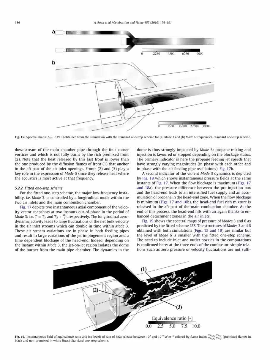
Fig. 15. Spectral maps (AFFT in Pa s) obtained from the simulation with the standard one-step scheme for (a) Mode 3 and (b) Mode 6 frequencies. Standard one-step scheme.


downstream of the main chamber pipe through the four cornervortices and which is not fully burnt by the rich premixed front(2). Note that the heat released by this last front is lower thanthe one produced by the diffusion flames of front (1) that anchorin the aft part of the air inlet openings. Fronts (2) and (3) play akey role in the expression of Mode 6 since they release heat wherethe acoustics is most active at that frequency.

5.2.2. Fitted one-step schemeFor the fitted one-step scheme, the major low-frequency insta-

bility, i.e. Mode 3, is controlled by a longitudinal mode within thetwo air inlets and the main combustion chamber.

Fig. 17 depicts two instantaneous axial component of the veloc-ity vector snapshots at two instants out-of-phase in the period ofMode 3: i.e. T ¼ T3 and T3 þ 3T3

2 , respectively. The longitudinal aero-dynamic activity leads to large fluctuations of the net bulk velocityin the air inlet streams which can double in time within Mode 3.These air stream variations are in phase in both feeding pipesand result in large variations of the jet impingement region and atime dependent blockage of the head-end. Indeed, depending onthe instant within Mode 3, the jet-on-jet region isolates the domeof the burner from the main pipe chamber. The dynamics in the

Fig. 16. Instantaneous field of equivalence ratio and iso-levels of rate of heat release beblack and non-premixed in white lines). Standard one-step scheme.

dome is thus strongly impacted by Mode 3: propane mixing andinjection is favoured or stopped depending on the blockage status.The primary indicator is here the propane feeding jet speeds thathave strongly varying magnitudes (in phase with each other andin phase with the air feeding pipe oscillations), Fig. 17b.

A second indicator of the violent Mode 3 dynamics is depictedby Fig. 18 which shows instantaneous pressure fields at the sameinstants of Fig. 17. When the flow blockage is maximum (Figs. 17and 18a), the pressure difference between the pre-injection boxand the head-end leads to an intensified fuel supply and an accu-mulation of propane in the head-end zone. When the flow blockageis minimum (Figs. 17 and 18b), the head-end fuel rich mixture isreleased in the aft part of the main combustion chamber. At theend of this process, the head-end fills with air again thanks to en-hanced detachment zones in the air inlets.

Fig. 19 shows the spectral maps of pressure of Modes 3 and 6 aspredicted by the fitted scheme LES. The structures of Modes 3 and 6obtained with both simulations (Figs. 15 and 19) are similar butthe level of Mode 6 is smaller with the fitted one-step scheme.The need to include inlet and outlet nozzles in the computationsis confirmed here: at the three ends of the combustor, simple rela-tions such as zero pressure or velocity fluctuations are not suffi-

tween 108 and 1010 W m�3 colored by flame indexrYC3 H8

�rYO2jrYC3 H8

:rYO2j (premixed flames in

Fig. 18. Instantaneous fields of pressure in the Y = 0 m and Z = 0 m planes. T3 stands for Mode 3: (a) maximum and (b) minimum of the flow blockage. Fitted one-step scheme.

Fig. 17. Instantaneous fields of non-dimensionalized axial component of the velocity vector in the Y = 0 m and Z = 0 m planes and iso-levels at U=Ubulk ¼ �0:05 in white andU=Ubulk ¼ 1 in dark. T3 stands for Mode 3: (a) maximum and (b) minimum of the flow blockage. Fitted one-step scheme.

Fig. 19. Spectral maps (AFFT in Pa s) obtained from the simulation with the fittedone-step scheme for (a) Mode 3 and (b) Mode 6 frequencies.


cient to ensure the exact evolution or selection of that acousticmode. The importance of Mode 3 and its impact on the dynamicsdescribed previously partly rely on the presence of a pressureanti-node standing within the head-end and the end of the air in-lets. This leads to variations of the mass flow rate at the end of theair inlets and at the beginning of the main combustion chamber asshown by Fig. 20. It shows the mass flux variations across planes inthe air and fuel feeding veins as well as in the main chamber pipe.Mean pressure signals recorded in these same planes and as a func-tion of time are also provided. Strong evolutions of both mass flow

rate and pressure (180� out-of-phase with one another) are evi-denced with up to, respectively, 40% and 15% variations. The max-imum of the flow blocage of the previous figures corresponds totime ta and the minimum to time tb.

Fig. 21 displays two instantaneous isovolumes of vertical veloc-ity (all points where the vertical component of the velocity vectoris more than 0:75� Ubulk or less than �0:75� Ubulk) and of rate ofheat release separated by half a period of Mode 3 from LES (left col-umn) and two snapshots obtained experimentally (right column).Periodically, zones of strong vertical velocity are released fromthe two air inlets and meet at the point of impingement of thetwo jets, Fig. 21a. The high-velocity sheet coming from theimpingement of the air inlet jets makes the four corner vortices cir-culation more intense and ensures the convection of the fuel out ofthe head-end. During this half period, the recirculation zone in thehead-end of the combustor gets stronger. The flame can not prop-agate but is pushed toward the outlet of the burner (Fig. 21a in LESand b in the experiment). When the flow blockage is minimum, i.e.when the air mass flow rate is minimum, the strong negative axialvelocities found both in the head-end of the chamber and on thetop and bottom sides of the impinging jets are released. The meanflow velocity in the chamber strongly decreases and the flame trav-els upstream against the main flow as evidenced in the experimenton Fig. 21d and LES on Fig. 21c. The corner vortices are almost ab-sent during this second phase, Fig. 21c. Note that when the flowblockage reaches its minimum, the flame can eventually propagateall the way to the central recirculation zone inside the head-end.This last phenomenon is linked to Mode 1.

These aerodynamic phenomena strongly influence the flamestabilization within a cycle of Mode 3. Fig. 22 shows that the flames

Fig. 20. Fluctuations of surface-averaged flow rate and pressure in three planes. Flow rates and pressures are normalized by their respective mean values. The planes are: (a)dark plane at the exit of the pre-injection box, (b) light gray plane at the exit of the upper air inlet and (c) dark gray plane upstream. Fitted one-step scheme.


stabilize downstream of the air inlet but that their position varieswith time and with the flow blockage. The variation of pressure in-duced by Mode 1 and Mode 3 can be such that the flame can reach

Fig. 21. Instantaneous fields using the fitted one-step scheme LES (left column) and seencomponent of velocity (0:75 Ubulk in white and �0:75 Ubulk in light gray) and the zero axialheat release (a hundredth of the maximum value) and shows where combustion takes plare direct images through a window starting 400 mm downstream of the air inlets sect

the central recirculation zone located in the head-end, Fig. 22b.Combustion regimes are also affected and vary in time. Fig. 23 pre-sents probability density functions of heat release rates versus

in the experiment (left column). In LES, the iso-volumes correspond to: the verticalcomponent of velocity in dark gray. The black iso-volume coincides with the rate of

ace. These views are taken within half a period apart in Mode 3. Experimental viewsions of the main chamber.

Fig. 22. Instantaneous fields of equivalence ratio in the Y ¼ 10�2 m and iso-levels of rate of heat release (from 108 to 1010 W m�3) colored by the flame indexrYC3 H8

�rYO2jrYC3 H8

�rYO2j

(premixed flames in black and non-premixed in white). Half a period of Mode 3, from the maximum (upper picture): T = 0 to the minimum (lower picture): T ¼ T32 of the flow

blockage. Fitted one-step scheme.


mixture fraction as constructed by ensemble averaging LES snap-shots at the instants of Fig. 22. Three peaks are clearly identified:

Fig. 23. Probability density function of local mixture fraction in reacting zonesdetected as zones where the local rate of heat release is higher than a 100th of thepeak value: (a) maximum and (b) minimum flow blockage. Fitted one-step scheme.

lean, rich and stoichiometric. When the maximum blockage occurs,stabilization of the combustion process is due to the propagation ofthe flames along the end of the corner vortices and the lean andrich peaks of Fig. 23a correspond to the fuel-lean and rich branchesof the flames as seen on Fig. 22 (upper picture). When the flowblockage decreases, fuel-rich pockets appear downstream of thechamber because of the increased strength of the corner vortices.These pockets are first consumed by the rich-premixed branchesof the former downstream propagating flames. The trailing diffu-sion flame is then convected along the flow with the pocket of pro-pane and toward the end of the chamber.

5.3. Impact of chemistry description on thermo-acoustic stabilitycriteria

A common tool used to assess thermo-acoustic stability ofburners is the Rayleigh criterion [66] which states that thermo-acoustic coupling occurs if pressure and heat release fluctuationsare in phase. Fig. 24 provides the spatial distribution of heat releasefluctuations in the Y ¼ 0 plane. Compared with spectral maps ofpressure shown on Figs. 15 and 19, only the simulation with thestandard one-step scheme allows such a coupling to appear at

Fig. 24. Standard deviation of reaction rate ðW mol�1 m�3Þ in the Y = 0 m plane and iso-levels between 500 and 1300 W mol�1 m�3: top, fitted one-step scheme and bottom,standard one-step scheme.


the frequency of Mode 6: heat release fluctuations obtained withthis LES are maximum at point (1) while they are weaker for thefitted one-step scheme where the maximum of fluctuations isfound downstream, at point (2). These last figures show why Mode6 is not selected in the fitted one-step scheme LES.

From the previous analyses and flow visualizations of the stan-dard one-step scheme predictions, Fig. 16, only front ð3Þ can beresponsible of such a constructive activity and is due to the wrongbehaviour of the chemical scheme at high equivalence ratios.

To conclude, the correction of the rich-side laminar flame speedintroduced in the fitted one-step scheme turns out to be necessaryto properly reproduce the thermo-acoustic behaviour of the exper-imental stato-reactor as reported by ONERA.

6. Conclusions

LES’s of the unsteady reacting flow in a side-dump combustorare produced with two different chemical schemes: a classicalone-step scheme and a similar scheme with a laminar flame speedthat is fitted to provide the proper behaviour at rich equivalenceratio values. For both cases, comparisons against measurementsshow very good agreement for mean velocity profiles. Howeverthe unsteady activity in the burner is correctly reproduced onlyin the second LES.

LES shows that combustion arises at places where the pressurenode of a longitudinal acoustic mode acts for the fitted one-stepLES while they occur at pressure nodes of a transverse acousticmode in the one-step LES. The simulation with the standard one-step scheme shows high-frequency oscillations (linked to thetransverse acoustic activity) but low-frequency oscillations are ob-served with the fitted one-step scheme. Strong coupling betweenheat release and pressure fluctuations is evidenced at these loca-tions which underlines thermo-acoustics as the driving mecha-nism in both cases. In this study, the excitation of the acousticmodes is eased by the chemical schemes that allow or preventcombustion of mixture at equivalence ratio above the rich flama-bility limit. In the first LES, rich premixed combustion can occurat the beginning of the corner vortices (in the head-end). Moregenerally, this study suggests that chemical schemes affect meanflow fields obtained by LES (something which is well-known) butalso the instabilities. It does not say, however, how precise thechemical scheme must be to capture these instabilities in general.For the present case, results show that fitting chemistry on the richside was sufficient for the ONERA ramjet but this may not be a gen-eral result. For this specific test rig, two other flight regimes whereonly the mass flow rate of fuel is changed have been studied (for aglobal equivalence ratio of 0.35 and 0.5). Experimental findings

show significant differences in flame positioning and mean reac-tion zones differ strongly from one test case to the other. Prelimin-ary LES results using the fitted scheme provide qualitatively goodagreement between experiments and simulations. Similarly tothe case studied in this work, the flame position and the form ofthe different mean reaction zones are well reproduced furtherillustrating that the chemical scheme is of prime order and that asimple fitting approach may offer a good alternative to complexchemical models. Such a method is however to be further validatedespecially in the context of flames whose position dependsstrongly on the temperature field and the burner heat transfer.

Acknowledgments

This research used resources of the Argonne Leadership Com-puting Facility at Argonne National Laboratory, which is supportedby the Office of Science of the U.S. Department of Energy undercontract DE-02-06CH11357 and access to the Centre InformatiqueNational de l’Enseignement Supérieur (CINES) in Montpellier,France, under the project FAC2554. A. Roux is supported financiallyby the French Délégation Général pour l’Armement (DGA). Sup-ports of DGA staff as well as M. Alain Cochet, head of the ‘‘Airbrea-thing Propulsion research unit” from the Fundamental and AppliedEnergetics Department of ONERA are gratefully acknowledged.

References

[1] N. Peters, B. Rogg, Reduced Kinetic Mechanisms for Applications inCombustion Systems, Lecture Notes in Physics, Springer Verlag, Heidelberg,1993.

[2] A. Ristori, G. Heid, C. Brossard, S. Reichstadt, in: XVIIth Symposium ISABE,Munich, Germany, 2005.

[3] G. Heid, A. Ristori, in: PSFVIP 4, CHAMONIX, France, 2003.[4] G. Heid, A. Ristori, in: ISABE, Munich, Allemagne, 2005.[5] A. Ristori, G. Heid, A. Cochet, G. Lavergne, in: XIVth Symposium ISABE,

Florence, Italy, 1999.[6] T. Poinsot, D. Veynante, Theoretical and Numerical Combustion, R.T. Edwards,

second ed., 2005.[7] H. Pitsch, Annu. Rev. Fluid Mech. 38 (2006) 453–482.[8] P. Moin, S.V. Apte, Am. Inst. Aeronaut. Astronaut. J. 44 (4) (2006) 698–708.[9] F. Ham, S.V. Apte, G. Iaccarino, X. Wu, M. Herrmann, G. Constantinescu, K.

Mahesh, P. Moin, in: Annual Research Briefs, Center for Turbulence Research,NASA Ames/Stanford Univ., 2003, pp. 139–160.

[10] S. James, J. Zhu, M. Anand, Am. Inst. Aeronaut. Astronaut. J. 44 (2006) 674–686.[11] G. Boudier, L.Y.M. Gicquel, T. Poinsot, D. Bissières, C. Bérat, Proc. Combust. Inst.

31 (2007) 3075–3082.[12] M. Boileau, G. Staffelbach, B. Cuenot, T. Poinsot, C. Bérat, Combust. Flame 154

(1–2) (2008) 2–22.[13] G. Boudier, N. Lamarque, G. Staffelbach, L. Gicquel, T. Poinsot, Int. J. Aeroacoust.

8 (1) (2009) 69–94.[14] G. Staffelbach, L. Gicquel, G. Boudier, T. Poinsot, Proc. Combust. Inst. 32 (2009)

2909–2916.


[15] L. Selle, G. Lartigue, T. Poinsot, R. Koch, K.-U. Schildmacher, W. Krebs, B. Prade,P. Kaufmann, D. Veynante, Combust. Flame 137 (4) (2004) 489–505.

[16] H. Pitsch, L.D. de la Geneste, Proc. Combust. Inst. 29 (2002) 2001–2008.[17] N. Patel, S. Menon, Combust. Flame 153 (1–2) (2008) 228–257.[18] S. Roux, G. Lartigue, T. Poinsot, U. Meier, C. Bérat, Combust. Flame 141 (2005)

40–54.[19] K. Kailasanath, J. Gardner, J. Boris, E. Oran, in: 22nd JANNAF Combustion

Meeting, 1985.[20] S. Menon, W. Jou, Combust. Sci. Technol. 75 (1–3) (1991) 53–72.[21] L.Y.M. Gicquel, Y. Sommerer, B. Cuenot, T. Poinsot, in: AIAA (Ed.), ASME 2006,

vol. Paper AIAA-2006-151, RENO, USA, 2006.[22] S. Reichstadt, N. Bertier, A. Ristori, P. Bruel, in: ISABE, 2007, p. 1188.[23] A. Roux, L.Y.M. Gicquel, Y. Sommerer, T.J. Poinsot, Combust. Flame 152 (1–2)

(2008) 154–176.[24] S.B. Pope, Combust. Theory Modell. 1 (1997) 41–63.[25] L. Lu, Z. Ren, V. Raman, S.B. Pope, H. Pitsch, in: Proc. of the Summer Program,

Center for Turbulence Research, NASA Ames/Stanford Univ., 2004, pp. 283–294.

[26] M.A. Singer, S.B. Pope, Combust. Theory Modell. 8 (2) (2004) 361–383.[27] B. Fiorina, O. Gicquel, L. Vervisch, S. Carpentier, N. Darabiha, Combust. Flame

140 (2005) 147–160.[28] O. Gicquel, N. Darabiha, D. Thevenin, Proc. Combust. Inst. 28 (1) (2009) 1901–

1908.[29] P. Domingo, L. Vervisch, S. Payet, R. Hauguel, Combust. Flame 143 (4) (2005)

566–586.[30] A. Vreman, B. Albrecht, J. van Oijen, P. de Goey, R. Bastiaans, Combust. Flame

153 (1) (2008) 394–416.[31] M.A. Singer, S.B. Pope, Combust. Theory Modell. 8 (2004) 361–383.[32] G. Ribert, O. Gicquel, N. Darabiha, D. Veynante, Combust. Flame 146 (4) (2006)

649–664.[33] S. Roux, M. Cazalens, T. Poinsot, J. Prop. Power 24 (3) (2008) 541–546.[34] B. Vreman, B. Geurts, H.H. Kuerten, Phys. Fluids 6 (12) (1994) 4057–4059.[35] P. Sagaut, Large Eddy Simulation for Incompressible Flows, Scientific

Computation Series, Springer-Verlag, 2000.[36] J.H. Ferziger, AIAA J. 15 (9) (1977) 1261–1267.[37] J. Smagorinsky, Mon. Weather Rev. 91 (1963) 99–164.[38] S.B. Pope, Turbulent Flows, Cambridge University Press, 2000.[39] P. Chassaing, Turbulence en mécanique des fluides, analyse du phénomène en

vue de sa modélisation à l’usage de l’ingénieur, Cépaduès-éditions, Toulouse,France, 2000.

[40] F. Nicoud, T. Poinsot, in: Int. Symp. On Turbulence and Shear Flow Phenomena.,Santa Barbara, September 12–15 1999.

[41] P. Moin, K.D. Squires, W. Cabot, S. Lee, Phys. Fluids A 3 (11) (1991) 2746–2757.

[42] G. Erlebacher, M.Y. Hussaini, C.G. Speziale, T.A. Zang, J. Fluid Mech. 238 (1992)155–185.

[43] F. Ducros, P. Comte, M. Lesieur, J. Fluid Mech. 326 (1996) 1–36.[44] P. Comte, New tools in Turbulence Modelling. Vortices in incompressible LES

and non-trivial geometries, Springer-Verlag, France, course of Ecole dePhysique des Houches, 1996.

[45] D.K. Lilly, Phys. Fluids 4 (3) (1992) 633–635. URL LES.[46] M. Germano, J. Fluid Mech. 238 (1992) 325–336.[47] S. Ghosal, P. Moin, J. Comput. Phys. 118 (1995) 24–37.[48] C. Meneveau, T. Lund, W. Cabot, J. Fluid Mech. 319 (1996) 353.[49] O. Colin, M. Rudgyard, J. Comput. Phys. 162 (2) (2000) 338–371.[50] F.A. Williams, Combustion Theory, Benjamin Cummings, Menlo Park, CA, 1985.[51] T.D. Butler, P.J. O’Rourke, in: 16th Symp. (Int.) on Combustion, The Combustion

Institute, 1977, pp. 1503–1515.[52] C. Angelberger, D. Veynante, F. Egolfopoulos, T. Poinsot, in: Proc. of the

Summer Program, Center for Turbulence Research, NASA Ames/Stanford Univ.,1998, pp. 61–82.

[53] C. Angelberger, F. Egolfopoulos, D. Veynante, Flow, Turb. Combust. 65 (2)(2000) 205–222.

[54] J.-P. Légier, T. Poinsot, D. Veynante, in: Proc. of the Summer Pro-gram, Centerfor Turbulence Research, NASA Ames/Stanford Univ., 2000, pp. 157–168.

[55] O. Colin, F. Ducros, D. Veynante, T. Poinsot, Phys. Fluids 12 (7) (2000) 1843–1863.

[56] C. Martin, L. Benoit, Y. Sommerer, F. Nicoud, T. Poinsot, AIAA J. 44 (4) (2006)741–750.

[57] P. Schmitt, T.J. Poinsot, B. Schuermans, K. Geigle, J. Fluid Mech. 570 (2007) 17–46.

[58] A. Sengissen, J.F.V. Kampen, R. Huls, G. Stoffels, J.B.W. Kok, T. Poinsot, Combust.Flame 150 (2007) 40–53.

[59] V. Moureau, G. Lartigue, Y. Sommerer, C. Angelberger, O. Colin, T. Poinsot, J.Comput. Phys. 202 (2) (2005) 710–736.

[60] T. Schönfeld, T. Poinsot, in: Annual Research Brie, Center for TurbulenceResearch, NASA Ames/Stanford Univ., 1999, pp. 73–84.

[61] S. Mendez, F. Nicoud, J. Fluid Mech. 598 (2008) 27–65. URL <http://www.cerfacs.fr/cfdbib/repository/TR_CFD_06_110.pdf>.

[62] A.W. Cook, W.H. Cabot, J. Comput. Phys. 203 (2005) 379–385.[63] J.-P. Légier, Simulations numériques des instabilités de combustion dans les

foyers aéronautiques, Phd thesis, INP Toulouse, 2001.[64] F. Hussain, J. Jeong, J. Fluid Mech. 285 (1995) 69–94.[65] P. Domingo, L. Vervisch, J. Réveillon, Combust. Flame 140 (3) (2005) 172–195.[66] A.A. Putnam, Combustion Driven Oscillations in Industry, Fuel and Energy

Science Series, j.m. beer ed., American Elsevier, 1971.

http://www.cerfacs.fr/cfdbib/repository/TR_CFD_06_110.pdf

http://www.cerfacs.fr/cfdbib/repository/TR_CFD_06_110.pdf

Analysis of unsteady reacting flows and impact of chemistry description in Large Eddy Simulations of...

Documents

Transcript of Analysis of unsteady reacting flows and impact of chemistry description in Large Eddy Simulations of...