Analysis of Preventive Maintenance in TransactionsBased Software SystemsSachin Garg1, Antonio Pulia�to2, Mikl�os Telek3, Kishor Trivedi11 Center for Advanced Computing & Communication.Department of Electrical Engineering, Duke UniversityDurham, NC 27708-0291 - USAE-mail: fsgarg,kstg@ee.duke.eduUrl: http://www.ee.duke.edu/�fsgarg,kstg2 Istituto di Informatica, Universit�a di CataniaViale A. Doria 6, 95025 Catania - ItalyE-mail: ap@iit.unict.it3 Department of TelecommunicationsTechnical University of Budapest1521 Budapest - HungaryE-mail: telek@pyxis.hit.bme.huAbstractPreventive maintenance of operational software systems, a novel technique for software faulttolerance, is used speci�cally to counteract the phenomenon of software \aging". However,it incurs some overhead. The necessity to do preventive maintenance not only in generalpurpose software systems of mass use but also in safety-critical and highly available systemsclearly indicates the need to follow an analysis based approach to determine the optimaltimes to perform preventive maintenance.In this paper, we present an analytical model of a software system which serves transac-tions. Due to aging, not only the service rate of the software decreases with time but thesoftware itself experiences crash/hang failures which result in its unavailability. Two policiesfor preventive maintenance are modeled and expressions for resulting steady state availabil-ity, probability that an arriving transaction is lost and an upper bound on the expectedresponse time of a transition are derived. Numerical examples are presented to illustrate theapplicability of the models.Keywords: Preventive Maintenance, Software Fault Tolerance, Transactions based Soft-ware Systems, Markov Regenerative Models. 1

1 IntroductionIt is now well established that system outages are caused more due to software faults thandue to hardware faults [24, 11]. Given the current growth in software complexity and reuse,the trend is not likely to change. It is also well known that regardless of development, testingand debugging time, software still contains some residual faults. Thus, fault tolerant softwarehas become an e�ective alternative to virtually impossible fault-free software. The scope ofthis paper lies in the quantitative evaluation of a novel technique for software fault tolerance,viz., preventive maintenance of operational software systems. Although, the use of preventivemaintenance is common in physical systems, its potential e�ectiveness in enhancing softwaredependability has only recently been recognized. As we shall exemplify later, in certainsituations, it is simply necessary.Traditional methods of software fault-tolerance, namely N-version programming [2], re-covery blocks [23] and N-self checking programming [19] are all based on design diversity,where independently operating teams of developers generate two or more variants of softwarefrom the same set of speci�cations. Another common characteristic in all of the above tech-niques is their reactive nature, i.e., the fault tolerance mechanism, or rather fault masking,takes e�ect after at least one version has experienced failure. The idea being that at leasta subset of the variants will not fail and therefore be collectively su�cient to provide thecorrect output. The primary drawback of all the above techniques is the extremely high costinvolved in generating multiple versions which restricts their use to safety-critical softwaresuch as for atomic power plants, railroad switching etc. [18], where the cost is justi�ed.Primarily, the following two factors motivate the need to explore alternate techniques forsoftware fault tolerance.1. Reliability/Availability Versus CostThe need for high reliability and availability is not just restricted to safety-critical sys-tems [11]. Telephone switches [7], airline reservation systems, process and productioncontrol, stock trading system, computerized banking etc. all demand very high avail-2

ability. A survey showed that computer downtime in non-safety critical systems costover 3:8 Billion in 1991 in U.S. [25]. With current explosive increase in the popularityof network centric computing, web servers too need to be highly available. In mostof these systems, the cost of providing fault tolerance via use of multiple variants isprohibitive. With commercial considerations driving technology more than ever, re-lease times of software are required to be less and less forcing organizations to reducetesting and debugging cycle times. Further, with software reuse gaining popularity,many times, it is simply not feasible to test the middleware and operating system onwhich the �nal software product is based. This leaves no option but to tolerate theresidual faults during its operational phase.2. Nature of software failuresMore recently, from the study of �eld failure data, it has been observed that a largepercentage of operational software failures are transient in nature [12, 13, 17], causedby phenomena such as overloads or timing and exception errors [24, 5]. A commoncharacteristic of these type of failures is that upon re-execution of the software, thefailure does not recur. The error condition, which results in the failure, typicallymanifests itself in the operating environment of the executing software. Due to thecomplexity of modern-day operating systems and intermediate layer software, it hasbeen observed that the same error condition, when the software is re-executed, isunlikely to recur, thus avoiding the failure.A study done by Adams implies that the best approach to masking software faults is tosimply restart the system [11]. Environment diversity, a generalization of restart, has beenproposed as a cheap yet e�ective technique for software fault-tolerance [15, 18]. Behaviorof a process (executing software) is determined by three components; the volatile state, thepersistent state and the Operating System (OS) environment. The volatile state consists ofthe program stack and static and dynamic data segments. Persistent state refers to all theuser �les related to a program's execution while the OS environment refers to resources thatthe program must access through the operating system, such as swap space, �le systems,3

communication channels, keyboard, monitors, time etc. [27]. Typical transient failures occurbecause of design faults in software which result in unacceptable erroneous states in theOS environment of the process. Therefore, the key idea behind environment diversity is tomodify the operating environment of the running process. Typically, this has been done ona corrective basis, i.e., upon a failure, the software is restarted after some cleanup, whichin most cases results in a di�erent, error free OS environment state thus avoiding furtherfailure.Recently, the phenomenon of software \aging" [16] has come to light where such errorconditions actually accrue with time and/or load. This observation has led to proposalsof a pro-active approach to environment diversity in which the operational software is oc-casionally stopped and \cleaned up" to remove any potential error conditions. Since thepreventive actions can be performed at suitable times (such as when there is no load onthe system), it typically results in lesser downtime and cost than the corrective approach.Even so, it incurs some overhead and if done more often than necessary will result in higherdowntime/cost. Therefore, an important research issue is to determine the optimal times toperform preventive maintenance of operational software systems.In this paper, we present a stochastic model for a transactions based software systemwhich employs preventive maintenance (henceforth referred to as PM). Three measures,availability of the software to provide service, probability of loss of a transaction and responsetime of a transaction are considered. The model is developed under very general conditionsand requires numerical solution. We compute each of the three measures under two policiesfor PM, which were proposed in [9], in the same framework. The rest of the paper is organizedas follows. In Section 2, we present real life examples of aging and PM to illustrate thedi�erent forms in which they occur and to motivate the need for analysis of such systems. InSection 3, we describe the system model, along with assumptions on modeling aging, failureand PM policies. Section 4 comprises of the analytical solution of the model for availability,loss probability and response time measures. In Section 5, we illustrate the usefulness of themodels via numerical examples. The two PM policies are compared along with the e�ect of4

model parameters on the derived measures. It is shown that the PM interval which maximizesavailability may be very di�erent from the PM interval which minimizes the probability ofloss or the response time, indicating caution in the selection of the optimum PM interval.Finally, in Section 6, we present the conclusions.2 Preventive Maintenance of Operational SoftwareWhile monitoring real applications, the phenomenon of software \aging" has been reported.It is observed that potential fault conditions slowly accumulate over time since the be-ginning of the software execution resulting in performance degradation and/or transientfailures1. Failures of both crash/hang type as well as those resulting in data inconsistencybecause of aging have been reported. Memory bloating and leaking, unreleased �le-locks,data corruption, storage space fragmentation and accumulation of roundo� errors are sometypical causes of slow degradation. Examples of aging can be found not only in software usedon a mass scale but also in specialized software used in high-availability and safety criticalapplications.Widely used web browser \Netscape" is known to su�er from serious memory leakingproblems which leads to occasional crash or hang of the application(s), especially in a com-puter with relatively low swap space. Similar memory leaking problem has been reportedin the news-reader program \xrn". All PC users are familiar with the occasional \switcho� and on" of the computer to recover from hangs. Such examples of aging in software ofmass-use are probably just an inconvenience, but in systems with high reliability/availabilityrequirements, software aging can result in high cost. Huang et. al. report this phenomenonin telecommunications billing applications where over time the application experiences acrash or a hang failure [16]. Avritzer and Weyuker have witnessed aging in telecommuni-cations' switching software where the e�ect manifests as gradual performance degradation1It should be noted that the term \software aging" was used in [1] to mean degradation in the quality ofthe software by an increase in number or severity of design faults due to repeated bug �xes, which is di�erentfrom our meaning. Perhaps in our context \process aging" is more appropriate, but we choose to keep theterm software aging to be consistent with the usage by Huang et. al.[16].5

[3]. The service rate of the software decreases with time increasing queue lengths and even-tually starts losing packets. Perhaps the most vivid example of aging can be found in [21],where the failure resulted in loss of human life. Patriot missiles, used during the Gulf war todestroy Iraq's Scud missiles used a computer whose software accumulated error. The e�ectof aging in this case was mis-interpretation of an incoming Scud as not a missile but just afalse alarm, which resulted in the death of twenty-eight U.S. soldiers.One way to counteract aging is to avoid the fault itself. Speci�cally, for memory leaks,commercially available packages like Purify and Insure++ exist. These, however, are for useduring the development phase with which memory leaks in a software can be detected andcorrected. Given that not all faults can be avoided (memory leakage is a very small subsetof faults resulting in aging) and that sometimes, it is simply not feasible to �x faults (useof third party software, unavailability of source code etc.), the complimentary approach oftolerating the residual faults must be employed. Moreover, the fault tolerance techniquemust not only be e�cient in terms of providing the necessary reliability or availability butmust be cost e�ective as well. Given the observed nature of failures, PM of operationalsoftware is a potential candidate.Huang et. al. [16] have proposed the technique of \Software Rejuvenation", which simplyinvolves stopping the running software occasionally, removing the accrued error conditionsand restarting the software. Garbage collection, ushing operating system kernel tables,reinitializing internal data structures are some examples of what cleaning the internal stateof a software might involve. An extreme, but well-known example of rejuvenation is a hard-ware reboot. It has been implemented in the real-time system collecting billing data formost telephone exchanges in the United States [4]. A very similar technique has been usedby Avritzer and Weyuker in a large telecommunications switching software [3], where theswitching computer is rebooted occasionally upon which its service rate is restored to thepeak value. They call it software capacity restoration. Both of the above independently usedtechniques are speci�c cases of PM performed on operational software. Grey [14] proposedperforming operations solely for fault management in SDI (Strategic Defense Initiative)6

software which are invoked whether or not the fault exists and called it \operational redun-dancy". Tai et. al. [26] have proposed and analyzed the use of on-board PM for maximizingthe probability of successful mission completion of spacecrafts with very long mission times.In a safety critical environment also, the necessity of performing PM is evident from theexample of aging in Patriot's software [21]. In the words of the author, On 21 February, theo�ce sent out a warning that \very long running time" could a�ect the targeting accuracy.The troops were not told, however, how many hours \very long" was, or that it would helpto switch the computer o� and on again after 8 hours.The concept of PM as such is not new. All system administrators, whether responsiblefor small system setup or for large commercial system setups such as banking, reservationssystems, inventory control systems etc. routinely perform PM, even if on an ad-hoc basis. Insome cases, it is performed on a per process basis, while in others a system wide maintenanceis done. In each case, however, the maintenance incurs an overhead which should be balancedagainst the cost incurred due to unexpected outage caused because of a failure. This in turndemands a quantitative analysis, which in the context of software systems has only recentlystarted getting attention. Mr. Bernstein stresses the need of emergence of a new �eld\software dynamics" [4] and calls for \developing the design constraints, analytically, tomake software behavior periodic and stable in its operational phase".The contribution of this paper lies in presenting an analytical model for transaction basedsoftware which experiences aging and employs PM to avoid unexpected outages. Further-more, two policies for PM are analyzed;1. Purely time based: PM is performed at �xed deterministic interval2. Time and load based: PM is attempted at �xed intervals and performed only if thesoftware is currently not serving any transactions.In both cases, equations for steady state availability, long run probability of a transactionloss and an upper bound on mean response time are derived.7

2.1 Previous WorkThe single most important factor (as shall be shown via numerical example) in determin-ing the accuracy of such a model is the assumptions made in capturing aging. Primarily,assumptions regarding the following aspects of aging need to be made.� E�ect of Aging: E�ect of aging has been witnessed as crash/hang failure, whichresults in unavailability of the software, and gradual performance degradation2. Userperceivable impact of one may be dominant than the other, but typically both arepresent to some degree in a software which experiences aging. In [16, 8, 9, 10, 26] onlythe failures causing unavailability of the software are considered, while in [22] considersonly a gradually decreasing service rate of a software which serves transactions isassumed. In this paper, we consider both the e�ects together in a single model.� Distribution: There is no consensus on the time to failure distribution of an opera-tional software and of the nature of service degradation it experiences. Therefore, forwide applicability, it is essential that a model be able to accommodate general distri-butions and not be restricted to predetermined ones. This way, with the availabilityof data, a speci�c distribution can then be applied on a per system basis. Modelsproposed in [16, 8, 9] are restricted to hypo-exponentially distributed time to failure.Those proposed in [10, 22, 26] can accommodate general distributions but only for thespeci�c aging e�ect they capture. In our model, we allow for generally distributed timeto failure as well as for the service rate to be an arbitrary function of time.� Dependence on Load: None of the previous studies capture the e�ect of load onaging. As it has been noted [24] that transient failures are partly caused by overloadconditions, in our model, we allow for the failure and the service rates to be functionsof time, instantaneous load, mean accumulated load or a combination of the above.2Incorrect output because of data inconsistency, from a modeling standpoint, can be captured in themodel for crash/hang failure since it is simply a failure at a speci�c time point8

Aging captured as: Model load Measure Evaluatedcrash/hang Performance general dependence? Availability Loss Response Completionfailure degradation distribution? Prob. Time Time Prob.[16] X X[8] X X[9] X X X[10] X X X[22] X X X[26] X X XOur X X X X X X XTable 1: Comparison of model assumptions and measures with previous workTable 1 summarizes the di�erences in capturing the e�ect of aging and on the assumptionsin the distribution and dependence of these e�ects in previous work. It also shows thedi�erences in the measures evaluated. In [10, 26] software with a �nite mission time isconsidered. Mean completion time in the presence of aging failures is computed in [10]whereas is [26], the probability of successful completion by the mission deadline is computed.In the rest [16, 8, 9] as well as in this paper, measures of interest in a transaction basedsoftware intended to run forever are evaluated. Where in [16] and [8], only the steady stateavailability is computed, both steady state availability as well as the long run probabilitythat a transaction is denied service are computed in [9]. In transaction based systems, theusers are sometimes more interested in response time. In this paper, we evaluate the steadystate availability, the probability of loss of a transaction as well as an upper bound on themean response time of a transaction. Optimizing one may result in an unacceptable valuefor the other. Optimal selection based on constraints on one or more of the measures canthen be made via solution of our model. Lastly, all previous models except [10] and [26] arejust special cases of the model presented in this paper.The rest of the paper deals with the proposed model, evaluation of the three measuresand numerical examples. 9

3 System ModelThe system we study consists of a server type software to which transactions arrive at aconstant rate �. Each transaction receives service for a random period. The service rate ofthe software is an arbitrary function measured from the last renewal of the software (becauseof aging) denoted by �(�). Therefore, a transaction which starts service at time t1, occupiesthe server for a time whose distribution is given by 1 � e� R tt1 �(�) dt. �(�) can be a constant,a function of time t, a function of the instantaneous load on the system, a function of totalprocessing done in a given interval or a combination of the above. We shall defer the explicitspeci�cation of the parameter in �(�) till Section 3.1.If the software is busy processing a transaction, arriving customers are queued. Totalnumber of transactions that the software can accommodate is K (including the one beingprocessed) and any more arriving when the queue is full are lost. The service discipline isFCFS. This state, in which the software is available for service (albeit with decreasing servicerate) is denoted as state \A" (see Figure 1).B

Rejuvenating

Recovering

Ava

ilabl

e

C

A

Figure 1: Macro-states representation of the software behaviorFurther, the software can fail upon which recovery procedure is started. This state, inwhich the software is recovering and is unavailable for service is denoted as state \B". Therate at which it fails, i.e., at which the software moves from state A to state B is denotedby �(�). Let the time to failure be denoted by random variable X. Then, its distribution is10

given by FX(t) = 1� e�R t0 �(�) dt:Like �(�), �(�) can also be function of time, instantaneous load, mean accumulated load or acombination of the above. Explicit speci�cation of �(�) shall be deferred till Section 3.1.The e�ect of aging, therefore, may be captured by using decreasing service rate andincreasing failure rate, where the decrease or the increase respectively can be a functionof time, instantaneous load, mean accumulated load or a combination of the above. Theservice degradation and hang/crash failures in our model are assumed to be stochasticallyindependent processes. Their interdependence, if it exists in the real system, can be ap-proximated by using parametric dependence in the de�nitions of �(�) and �(�). The failureprocess is stochastically independent of the arrival process and any transactions in the queueat the time of failure are assumed to be lost. Moreover, any transactions which arrive whilerecovery is in progress are also lost. Time to recover from a failed state is denoted by Yfwith associated general distribution FYf .Lastly, the software occasionally undergoes PM. This state is denoted as state \C". PMis allowed only from state \A". We consider two di�erent policies which determine the timeto perform PM.1. Purely time based. Under this policy, henceforth referred to as Policy I, PM is initiatedafter a constant time � has elapsed since it was started (or restarted). We shall referto � under this policy as the PM interval.2. Instantaneous load and time based. Under this policy, henceforth referred to as PolicyII, a constant waiting period � must elapse before PM is attempted. Further, after thistime, PM is initiated if and only if there are no transactions in the system. � underthis policy shall be referred to as PM wait. The actual PM interval under Policy II isdetermined by the sum of PM wait and the time it takes for the queue to get emptyfrom that point onwards. The latter quantity is dependent on system parameters andcan not be controlled. The actual PM interval, therefore has a range [�;1).11

Regardless of the policy used, it takes a random amount of time, denoted by Yr, toperform PM. Let FYr be its distribution. As will be showed in the following section, ourmodel does not require any assumptions on the nature of FYf and FYr . Only the respectiveexpectations f = E[Yf ] and r = E[Yr] are assumed to be �nite.Once recovery from the failed state or PM is complete, the software is reset in state Aand is as good as new. From this moment, which constitutes a renewal, the whole processstochastically repeats itself. The transition behavior of the software among states A, B andC is illustrated in Figure 1.The queuing behavior of the software, on the other hand, as determined by the two PMpolicies is illustrated in Figure 2. The horizontal axis represents time t and the vertical axisrepresents the number of transactions queued in the software at time t, denoted by N(t).Figure 2(a) shows a sample path in which PM is initiated as soon constant time � elapses.In accordance with Policy I, the transactions already in the queue at time � are lost.Figure 2(b) illustrates Policy II where at time �, some transactions are in the queue ,i.e., N(�) > 0. In this case, the software waits till the queue is empty upon which PM isinitiated3 This wait is a random quantity denoted in the �gure by B. Intuitively, if B is verylarge, it is likely that the software will fail before it has a chance to undergo PM.Given the above behavioral model, for each policy, we need to:1. Evaluate the steady state availability of the software2. Evaluate the steady state probability that an arriving transaction will be denied service.3. Evaluate the expected response time of a transaction successfully served.4. Determine optimal values of � (PM interval under policy I and PM wait under policyII) which provide optimal values for steady state availability, long run probability ofloss and expected response time.3A generalization of Policy II in which after time � PM is initiated if and only if the number of transactionsin the queue goes below a certain threshold can easily be accommodated in our model.12

RE

JUV

EN

AT

ION

rγδ B t

N(t)

N(t)

tδ

RE

JUV

EN

AT

ION

γr

(a)

(b)Figure 2: Sample Path of the process3.1 How to Capture Aging?The e�ect of aging, i.e., degradation in performance and failures causing unavailability arepresent in varying severity in di�erent systems. Further, each of them may be in uencedby di�erent operating parameters in di�erent software systems. We now show how, in ourmodel, the varying severity and dependencies may be captured via proper choice of param-eters of �(�) and �(�). Flexibility in this choice in the same framework widens the scope ofapplicability of our model to real software systems.� �(�) = � and �(�) = �.In the simplest case, the service rate as well as the failure rate are constants. Thisimplies that there is no performance degradation and the time to failure is exponentiallydistributed, which because of its memoryless property contradicts aging. Therefore,constant � and � do not capture the behavior of a software system which ages. Thiscase will not be discussed further.� �(�) = �(t) and �(�) = �(t)In this case, the service rate and the failure rates are simply functions of time. Althougharbitrary functions are allowed in the model, presumably, service rate will be a mono-13

tone non-increasing function and the failure rate will be a monotone non-decreasingfunction of time in a software which ages. If�(t) = ��t��1where � and � are constants with � > 1, the time to failure has Weibull distributionwith increasing failure rate, which is commonly used to model aging. To model softwaresystems where only occasional failures are witnessed with no performance degradation,the combination �(�) = � and �(�) = �(t) may be used. Further, to model softwaresystems which undergo performance degradation but are always available, the specialcase of �(�) = � = 0 and �(�) = �(t) can be used.� �(�) = �(N(t)) and �(�) = �(N(t))The service rate and the failure rate are functions of instantaneous load on the system,i.e., their value at time t depends on the number of transactions in the queue atthat time. This dependence is useful in capturing overload e�ects which in uence thefailure behavior especially. Of course, more realistic combined dependence on time andinstantaneous load, �(�) = �(t; N(t)) and �(�) = �(t; N(t)) is also allowed.� �(�) = �(L(t)) and �(�) = �(L(t))A more complex but also more powerful dependence can be obtained by making �(�)and �(�) as functions of mean accumulated work done by the software system in a giventime interval. Let pi(t); 0 � i � K be the probability that there are i transactions inthe queue at time t given that the software is in state \A". When the software is notaged, incoming transactions are promptly served and the total amount of time spentin actual processing in an interval (0; t] is usually less than the interval t itself. Since,an idle software is not likely to age, service and failure rates are more realistically afunction of the actual processing time rather than the total available time. Let L(t)be de�ned as: L(t) = Z t�=0Xi cipi(�)d�14

where ci is a coe�cient which expresses how being in state i in uences the degradationof the overall system. If c0 = 0 and ci = 1 for i > 0 then L(t) represents the averageamount of time the software is busy processing transactions in the interval (0; t]. ifci = 1 for i � 0, then L(t) = t given that the software is available.Lastly, our model allows for combination of above dependencies. For example, thefailure rate may be a function of not only the mean processing time in the interval(0; t], but also of the instantaneous load at time t to account for overload e�ects. Inthis case, �(�) = �(N(t); L(t)).In the following section, we derive the three measures for the two PM policies. Table 2lists the notation used in the rest of the paper. (R.V. denotes random variable):PAB Transition probability from state A (Available) to state B (Recovering)PAC Transition probability from state A (Available) to state C (Undergoing PM)pi(t) Probability that i transactions are queued at time t,Nl Number of transactions lost at the end of theavailable period (R.V.) f Expected time to recover from failure r Expected time to perform PMU Sojourn time in state A (R.V.)� Transaction arrival rate�(�) Transaction service rate�(�) Failure rateN(t) Number of transaction in the queue at time tL(t) Mean processing time since the last renewalTable 2: Notation4 Evaluation of MeasuresLet the steady state availability of the software system be denoted by ASS. Let Ploss denotethe long run probability that an arriving transaction will be lost and let Tres denote theexpected response time of a transaction given that it is successfully served. The approach15

we follow in deriving the expressions for the three measures applies to both policies I andII. Only when a particular expression is di�erent, it will be noted explicitly. The solutionmethod in general, and the class of stochastic process used to model in particular, provides anelegant, concise and fast alternative to usually expensive discrete-event simulation approach.As described in the previous section, the software can be in any one of three states at anytime t. It can be up and available for service (state A), recovering from a failure (state B)or undergoing PM (state C) (see Figure 1). Let fZ(t); t � 0g be a stochastic process whichrepresents the state of the software at time t. Further, let the sequence of random variablesSi; i > 0 represent the times at which transitions among di�erent states take place. Then,fZ(Si); i > 0g is an embedded discrete time Markov chain (DTMC), since the entrance timesSi constitute renewal points. The transition probability matrix P for this DTMC can beeasily derived from the state transition diagram shown in Figure 1 and is given by:P = 0B@ 0 PAB PAC1 0 01 0 0 1CA (1)The steady state probability of the software being in state i; i 2 fA;B;Cg, denoted bypi, can also be determined in a straightforward manner from the well know relation � = �P .These probabilities are given by; �A = 12�B = 12PAB (2)�C = 12PACThe software behavior as a whole is modeled via the stochastic process f(Z(t); N(t)) ; t �0g. If Z(t) = A, then N(t) 2 f0; 1; : : : ; Kg, as the software queue can accommodate upto K transactions. If Z(t) 2 fB;Cg, then N(t) = 0, since by assumption, all transactionsarriving while the software is either recovering or undergoing PM are lost. Further, thetransactions already in the queue at the transition instant are also discarded. It can beshown that the process f(Z(t); N(t)) ; t � 0g is a Markov regenerative process (MRGP) [6].16

The regeneration instants are embedded at times when the process makes transitions fromstate i to state j (i; j 2 fA;B;Cg), i.e. Z(t) changes. Transition to state A from either B orC constitutes a regeneration instant since by assumption, the software is reset to the originalinitial conditions. At these instants, the system in empty and the software is as good as new.Note that what makes the process an MRGP is the fact that within one regeneration period,the stochastic process changes state. In other words, arrivals and departures of transactionskeep changing N(t) while Z(t) = A. We have already de�ned and solved the embeddedDTMC of this MRGP in Equations (1) and (3) respectively.Let U be a R.V. denoting the sojourn time of f(Z(t); N(t)); t > 0g in state A. Let E[U ]denote its expectation. Expected sojourn times of the MRGP in states B and C are alreadyde�ned to be given by f and r. The steady state availability can then be obtained usingstandard formulae from MRGP theory [6] and is given as:ASS = Prfsoftware is in state Ag = �AE[U ]�B f + �C r + �AE[U ]Substituting the values of �A, �B and �C ,ASS = E[U ]PAB f + PAC r + E[U ] (3)The probability that a transaction is lost is de�ned as the ratio of expected number oftransactions which are lost in an interval to the expected total number of transactions whicharrive during that interval. The evolution of fZ(t); N(t)); t > 0g in the intervals comprisingof successive visits to state A is stochastically identical. Therefore, for calculation of long runmeasures, it su�ces to consider just one such interval. The expected number of transactionslost is the given by the summation of three quantities; (1) the expected number lost due todiscarding because of failure or initiation of PM, (2) the expected number lost while recoveryor PM is in progress and (3) the expected number lost due to the bu�er being full. Thelast quantity is of special signi�cance as due to the degrading service rate, the probabilityof bu�er being full increases.17

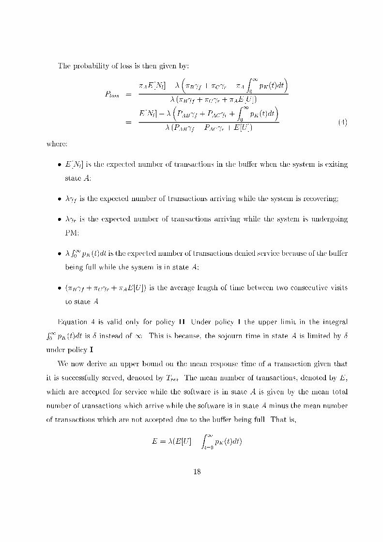
The probability of loss is then given by:Ploss = �AE[Nl] + ���B f + �C r + �A Z 10 pK(t)dt�� (�B f + �C r + �AE[U ])= E[Nl] + ��PAB f + PAC r + Z 10 pK(t)dt�� (PAB f + PAC r + E[U ]) (4)where:� E[Nl] is the expected number of transactions in the bu�er when the system is exitingstate A;� � f is the expected number of transactions arriving while the system is recovering;� � r is the expected number of transactions arriving while the system is undergoingPM;� � R10 pK(t)dt is the expected number of transactions denied service because of the bu�erbeing full while the system is in state A;� (�B f + �C r + �AE[U ]) is the average length of time between two consecutive visitsto state A.Equation 4 is valid only for policy II. Under policy I the upper limit in the integralR10 pK(t)dt is � instead of 1. This is because, the sojourn time in state A is limited by �under policy I.We now derive an upper bound on the mean response time of a transaction given thatit is successfully served, denoted by Tres. The mean number of transactions, denoted by E,which are accepted for service while the software is in state A is given by the mean totalnumber of transactions which arrive while the software is in state A minus the mean numberof transactions which are not accepted due to the bu�er being full. That is,E = �(E[U ]� Z 1t=0 pK(t)dt)18

Out of these transactions, on the average, E[Nl] are discarded later because of failure andinitiation of PM. Therefore, the mean number of transactions which actually receive servicegiven that they were accepted is given by E � E[Nl]. The mean total amount of time thetransactions spent in the system while the software is in state A is:W = Z 1t=0Xi ipi(t) dtThis time is composed of the mean time spent by the transactions which were served as well asthose which were discarded, denoted asWS andWD, respectively; Therefore, W = WS+WD.The response time we are interested in is given byTres = WSE � E[Nl] :which is upper bounded by4 Tres < WE � E[Nl] : (5)Regardless of the PM policy, as can be observed from Equations (3) and (4), we need toobtain expected sojourn times and the steady state probability of the software in each of thethree states A;B and C, as well as the transient probability that there are i; i = 0; 1; : : : ; Ktransactions queued up for service. It is the last quantity which forbids a closed formanalytical solution and necessitates a numerical approach.The mean sojourn time in states B and C is already available as f and r respectively5.The quantities still to be derived are related with the queuing behavior of the software instate A, viz., PAB, PAC , E[U ] and pi(t); i = 0; 1; : : : ; K. Their evaluation depends on thepolicy used.4.1 Behavior of the system in state A under Policy IFor Z(t) = A, the subordinated process, i.e., the process until a regeneration occurs, isdetermined by the queuing behavior of the software processing transactions. The process is4 WE�E[Nl] tends to WSE�E[Nl] as E[Nl]E tends to 0.5The measures evaluated in this paper require only the �rst moments of Yf and Yr and hence no assump-tions on the nature of their distribution is made. 19

terminated by either a failure (which can happen at any time) or by initiating PM whichunder policy I happens at time � if the software has not failed by that time. Figure 3shows the state diagram of the subordinated non-homogeneous process under policy I. It isa birth-death process augmented with one absorbing state associated with each state of thebirth-death process. Not included in the �gure is the fact that at t = �, the subordinatedprocess is terminated if it was not terminated before by a transition to an absorbing state(00; : : : ; K 0).ρ( )L(t) ρ( )L(t)

µ( )L(t) µ( )L(t) µ( )L(t) µ( )L(t)

ρ( )L(t) ρ( )L(t) ρ( )L(t) ρ( )L(t)

λλλ λ

’ ’ ’210

3

3’ ’K-1 K’

0 1 2 K-1 K

Figure 3: Subordinated Non-homogeneous CTMC for t � �By our notation, pi(t) is the probability that there are i transactions queued for service,which is also the probability of being in state i of the subordinated process at time t. Notethat state i; i = 0; 1; : : : ; K is not to be confused with state i0; i = 0; 1; : : : ; K which wasde�ned just to be able to evaluate the quantities of interest. As such, all the states underthe shaded area of the process can be lumped into a single absorbing state.pi(t); i = 0; 1; : : : ; K and pi0(t); i0 = 00; 10; : : : ; K 0 can be obtained by solving the followingsystem of forward di�erential-di�erence equations:dp0(t)dt = �(�)p1(t)� (�+ �(�)) p0(t)dpi(t)dt = �(�)pi+1(t) + �pi�1(t)� (�(�) + �+ �(�)) pi(t); 1 � i < KdpK(t)dt = �pK�1(t)� (�(�) + �(�)) pK(t) (6)dpi0(t)dt = �(�)pi(t); 0 � i � K 20

�(�) and �(�) can have any of the forms described in Section 3.1. If �(�) = �(t) or �(N(t))and �(�) = �(t) or �(N(t)), no other changes except for plugging in the proper values isnecessary. For �(�) = �(L(t)) and �(�) = �(L(t)), where L(t) is de�ned byL(t) = Z t�=0Xi cipi(�)d�;the set of ODEs is �rst augmented by the following di�erential equation.dL(t)dt =Xi cipi(t)and then solved.The set of simultaneous di�erential-di�erence equations given by (6) do not in generalhave a closed-form analytical solution and must be evaluated numerically along with theinitial conditions p0(0) = 1, pi(0) = 0; 1 � i � K and pi0(0) = 0; 00 � i0 � K 0. Once theseprobabilities are obtained, the rest of the quantities can be computed as follows.One step transition probability PAB is given by:PAB = K0Xi=00 pi(�)and PAC = 1� PABThereafter, according to Equation (3), the steady state probability that the software is instates B and C can be obtained.The expected sojourn time in state A is given by:E[U ] = Z �t=0 KXi=0 pi(t)! dtwhere the upper limit on the integral indicates that the sojourn time is bounded by �. Theaverage value, E[Nl], of the number of transactions already in the system at the time whenstate A is left, is evaluated as: E[Nl] = KXi=0 i (pi(�) + pi0(�))ASS, Ploss and the upper bound on Tres as given in Equations (3), (4) and (5) respectivelycan now be easily calculated. 21

4.2 Behavior of the System in State A Under Policy IIIf policy II is assumed, the evolution of the system in state A is somewhat more complex. Inthis case we need to distinguish between t � � and t > �, as policy II assumes that PM willbe initiated if and only if the bu�er is empty after time � has elapsed. For t � �, exactlythe same process of Figure 3 determines the behavior of the software. For t > �, the processwhich models the behavior is shown in Figure 4. As can be observed, state 0 now belongs tothe set of absorbing states because PM will be initiated once the system becomes idle thusterminating the subordinated process,µ( )L(t) µ( )L(t) µ( )L(t)

ρ( )L(t) ρ( )L(t) ρ( )L(t) ρ( )L(t) ρ( )L(t)

λλ λ

L(t)µ( )

3

3’ ’ ’ ’K-1 K’21

1 2 K-1 K0

Figure 4: Subordinated Non-homogeneous CTMC if t > �The set of forward di�erential-di�erence equations which are solved to determine alltransient probabilities are given as follows:dp0(t)dt = �(:)p1(t)� (�0(t) + �(:)) p0(t)dp1(t)dt = �(:)p2(t) + �0(t)p0(t)� (�(:) + �+ �(:)) p1(t);dpi(t)dt = �(:)pi+1(t) + �pi�1(t)� (�(:) + � + �(:)) pi(t); 2 � i < KdpK(t)dt = �pK�1(t)� (�(:) + �(:)) pK(t) (7)dp00(t)dt = �0(:)p0(t)dpi0(t)dt = �(:)pi(t); 1 � i � Kwhere �0(t) = �, if t � �, otherwise it is zero. Similarly, �0(:) = �(:), if t � �, otherwise22

zero. As before, �(�) and �(�) can be functions of t, N(t) or L(t), where in the last case, theset of ODEs must be augmented withdL(t)dt =Xi cipi(t)and then solved. This set of di�erential-di�erence equations along with the initial conditionp0(0) = 1 also requires numerical solution.On step transition probability PAB is computed by solving the system of ODEs at t =1and is given as: PAB = K0Xi=00 pi(1):Then PAC = 1� PAB = p0(1):The mean sojourn time in state A is now given by:E[U ] = Z �t=0 KXi=0 pi(t)! dt+ Z 1t=� KXi=1 pi(t)! dt= Z �t=0 p0(t)dt+ Z 1t=0 KXi=1 pi(t)! dtThe mean number of transactions already in the queue the State A is exited is given by:E[Nl] = KXi=0 i pi0(1):Using Equations (3), (4) and (5), the steady state availability, the probability of loss of anarriving transaction and the upper bound on the response time of a transaction can now becalculated.5 Numerical ExamplesIn this section, we illustrate the usefulness of the models developed to evaluate ASS, Plossand the upper bound on Tres. The models are solved for multiple values of � (PM interval inthe case of policy I and PM wait in the case of policy II) and optimal values are determined.23

We also show, how the optimum value of � may be selected based on combined measures ofthe above three quantities.Table 3 shows the parameter values that were kept �xed for all results. The values chosenare for illustration purposes only and do not necessarily represent any physical system. f 0:85 (hours)� 6:0 (hours�1)K 50MTTF 240 (hours)Table 3: Model parametersThe set of di�erential-di�erence equations given in Equations (6) and (8) for policies Iand II respectively were numerically solved using the LSODE routine in ANSI FORTRAN.LSODE (Livermore Solver for Di�erential Equations) is an ODE solver which uses Backwarddi�erentiation Formula (BDF) methods for sti� systems of ODEs. It is publicly available aspart of ODEPACK from netlib. A single run of the model takes less than a minute. Solutionusing commercially available packages like Mathematica or MATLAB is also possible, butis likely to be much slower. For large bu�er sizes of the order of thousands, sparse matrixmethods will need to be used in the ODE solution.5.1 Experiment 1.In this experiment, r is varied to ascertain the e�ect on the measures and on optimal �.Service rate and failure rate are assumed to be functions of real time, i.e., �(�) = �(t) and�(�) = �(t), where �(t) is de�ned to be�(t) = ��t��1;which is the hazard function of Weibull distribution. � is �xed at 1:5 and � is calculatedfrom the MTTF and � as � = "�(1 + 1�)MTTF #� (8)24

The model is solved for both policies to show the e�ect of the cost of PM on the threemeasures. �(t) is de�ned to be a monotone non-increasing function of t as shown in Figure 5.This behavior of �(t) has been given in [3] as an approximation to service degradation intelecommunications switching software.µ max

µ min

aFigure 5: Time variation of the service rate �(t)�max is �xed at 15 hour�1 and �min at 5 hour�1 for all the experiments in the paper.For this particular experiment of varying r, �(t) (as shown in Figure 5) is de�ned as:�(t) = ( �max h1� tMTTF i ; if t � a�min; if t > awhere a = (�max � �min)�max MTTF:The use of common parameterMTTF in the de�nitions of �(t) and �(t) is simply to illustratehow dependence in the service and failure behavior can be captured via parameter sharing,even though stochastically the two processes are assumed to be independent.In the numerical evaluation of the measures, computation at time1 is required which isapproximated by respective values at time tMAX where tMAX is associated with the requiredprecision parameter (�) by the following expression:FX(tMAX) = Z tMAX0 Xi pi(t) dt = 1� �:Figure 6(a) shows Ass plotted against di�erent values of � for both PM policies I and II.Further, for each policy, r was assigned values of 0:15, 0:35, 0:55 and 0:85 hours. Asnoted already, the expected downtime due to a failure is kept �xed at 0:85 hours. Under25

0.0 100.0 200.0 300.0 400.0δ

0.990

0.991

0.992

0.993

0.994

0.995

0.996

0.997

0.998A

vaila

bilit

y

I, 0.15I, 0.35I, 0.55I, 0.85II, 0.15II, 0.35II, 0.55II, 0.85

0.0 50.0 100.0 150.0δ

0.00

0.01

0.01

0.02

0.02

0.03

0.04

Los

s Pr

obab

ility

I, 0.15I, 0.35I, 0.55I, 0.85II, 0.15II, 0.35II, 0.55II, 0.85

Figure 6: Results for Experiment 1.both policies, it can be seen that higher the value of r, lower is the availability for anyparticular value of �. Under policy I, for r = 0:15 and r = 0:35, the availability rapidlyincreases with increase in � (that is PM is performed less frequently), attains a maximumat � = 160 and � = 410 respectively and then gradually decreases. For r = 0:55 and r = 0:85, the steady state availability turned out to be a monotone function. In all cases,Ass eventually approaches the same value with increase in � which corresponds to the steadystate availability if no PM was performed. Therefore, for r = 0:55 and r = 0:85, it is betternot to perform PM, if the objective is only to maximize availability. Under policy II, thesteady state availability follows the same behavior as in policy I except that the value of Asscorresponding to the no PM case is reached at much lower values of �, which now representsPM wait rather than the PM interval.Figure 6(b) shows the plots of Ploss against � for both policies with r being assignedvalues as in Figure 6(a). All the plots attain a minimum. As expected, for any speci�c valueof � and a speci�c policy, higher is the value of r, higher is the corresponding loss probability,because on average, more transactions are denied service while PM is in progress. Since theabsolute values of the measures or of optimal � are not of importance, we shall comment onthe relative e�ects only. It can be seen that for any speci�c policy, lower the value of r,lower is the value of � which minimizes the probability of loss for that particular r. For anyspeci�c value of r, policy II results in a lower minima in loss probability than that achieved26

under policy I. Moreover this minima under policy II is achieved at a lower � as comparedto policy I. This clearly shows that if the objective is to minimize long run probability ofloss, which is the case is telecommunication switching software, policy II always fares betterthan policy I. It can also be observed from Figure 6(a) and 6(b), that the value of � whichminimizes probability of loss is much lower than the one which maximizes availability. Infact, the probability of loss becomes very high at values of � which maximize availability.Although the behavior is dependent on system parameter values, caution in proper selectionof � is indicated.5.2 Experiment 2In this experiment, r is �xed at 0:15. �(�) = �(t) and has exactly the same de�nition asin Experiment 1. �(�) = �(t), with previously de�ned Weibull hazard rate, except that theshape parameter � is now varied. Thus for each value of �, corresponding � is calculatedusing Equation (8) keepingMTTF �xed at 240 hours. In e�ect, we are interested in studyinghow the measures and the optimality varies as the failure density gets peakier with the samemean time to failure. � is assigned values of 1:0, 1:5 and 2:0 respectively.Figure 7(a) shows the steady state availability under the two policies plotted against �for di�erent values of �.

0.0 100.0 200.0 300.0 400.0δ

0.990

0.991

0.992

0.993

0.994

0.995

0.996

0.997

0.998

Ava

ilabi

lity

I, 1.0I, 1.5I, 2.0II, 1.0II, 1.5II, 2.0

0.0 50.0 100.0 150.0δ

0.00

0.01

0.01

0.02

0.02

0.03

0.04

Los

s Pr

obab

ility

I, 1.0I, 1.5I, 2.0II, 1.0II, 1.5II, 2.0

Figure 7: Results for Experiment 2.27

For � = 1:0, the time to failure has an exponential distribution, which, because of itsmemoryless property, contradicts aging. As seen from the �gure, it is better not to performPM in this case, if the objective is to maximize availability. For the other two values of �,however, PM maximizes availability at certain �. For a speci�c policy, peakier the failuredensity, i.e., higher the value of �, higher is the maximum steady state availability. Secondly,with higher values �, this maxima occurs at lower values of �. Figure 7(b) shows the longrun probability of loss of a transaction plotted against �. In this case, PM proves to bebene�cial for all three values of �. Similar observations and arguments as those given inExperiment 1 hold for this case also.5.3 Experiment 3The purpose of this experiment is to illustrate the e�ect of assumptions on �(�) and �(�)on the three measures. Figure 8(a), (b) and (c) show steady state availability, probabilityof loss and the upper bound on the mean response time of transactions successfully servedplotted against � under policy I.0 100 200 300 400 500

δ

0.990

0.992

0.995

0.997

1.000

Ava

ilabi

lity

real timeBusy timeno failure

0 100 200 300 400 500δ

0.00

0.03

0.05

0.08

0.10

Los

s Pr

obab

ility

real timebusy timeno failure

0 100 200 300 400 500δ

0.0

1.0

2.0

3.0

4.0

5.0

6.0

Res

pons

e T

ime real time

busy timeno failure

Figure 8: Results of Experiment 3.Each of the �gures contains three curves. The solid curve represents a system where�(�) = �(t) and �(�) = �(t). The dotted curve represents a second system where �(�) =�(L(t)) and �(�) = �(L(t)). The parameters, �max, �min and a are kept the same. Similarly,� is kept at 1:5 for both the solid as well as the dotted curve. In other words, �(�) and �(�)in the solid curve are functions of real time, whereas in the dotted curve, they are functions28

(with the same parameters) of the mean total processing time. The dashed curve representsa third system in which no crash/hang failures occur, i.e., �(�) = 0 but service degradationis present with �(�) = �(t) with same parameters as for �(�) of earlier two systems. r forall is kept �xed at 0:15, This experiment only illustrates the importance of making the rightassumptions in capturing aging because as seen from the �gure, depending on the formschosen for �(�) and �(�), the measures vary in a wide range.Figure 8 plots the upper bound on the mean response time. This was not shown forExperiments 1. and 2. because of its monotone nature. In the type of system underconsideration, where queued transactions as well as those arriving during recovery or PM arelost, response time of successful transactions can be trivially minimized by always keeping thesoftware unavailable (with very low �). This however, will result in unacceptable values of theprobability of loss and steady state availability. In many systems, for example ATM switches,QOS requirements are speci�ed using bounds on response time as well as probability of loss.This can be achieved via our model. For example, consider the solid curve in Figure 8(c). IfQOS demands that the response time be less than 0:113 hours, � is restricted approximatelyin the interval (0; 70]. Now, if the QOS further demands that the probability of loss beminimized, the optimal � corresponds to the minimum Ploss within this interval only. Thecurve identi�ed with the legend (I,1.5), in Figure 7(b) plots Ploss against � with exactly thesame parameter values and it is seen that global minima for Ploss occurs at � = 85 whereasthe optimal � for the combined QOS is 70.6 ConclusionIn this paper, we motivated the need of pursuing preventive maintenance in operationalsoftware systems on a scienti�c analytical basis rather than the current ad-hoc practice.We presented a model for a transactions based software system which employs preventivemaintenance to either maximize availability, minimize probability of loss, minimize responsetime or optimize a combined measure. We evaluated the three measures for two di�erentpreventive maintenance policies and showed via numerical examples that a policy which takes29

into account instantaneous load on the system results in lower optimum probability of loss.The e�ect of aging is captured as crash/hang failures as well as performance degradation.Systems which experience only one of the two can be modeled as special cases. The mainstrength of our model, however, is its capability of capturing the dependence of crash/hangfailures and performance degradation on time, instantaneous load, mean accumulated loador a combination. This, in our opinion, provides great exibility in modeling real situationsand widens the scope of applicability of our model. The main limitation, on the other hand,is that it is applicable to only those software systems in which incoming transactions arelost when either it fails or when PM in initiated. In many database systems which supportrecovery, transactions are logged when they arrive. Even when failure occurs, the log is notlost, thus violating our assumption.References[1] E. Adams, \Optimizing preventive service of the software products", IBM J. R&D,28(1), Jan, 1984, pp. 2-14.[2] A. Avizienis, \The n-verion approach to fault-tolerant software", IEEE Trans. on Soft-ware Engg., Vol. SE-11, No. 12, pp. 1491-1501, December 1985.[3] A. Avritzer and E. J. Weyuker, \Monitoring smoothly degrading systems for increaseddependability", submitted for publication.[4] L. Bernstein, Text of seminar delivered by Mr. Bernstein, University Learning Center,George Mason University, January 29, 1996.[5] R. Chillarege, S. Biyani and J. Rosenthal, \Measurements of failure rate in commercialsoftware", in Proc. of 25th Symposium on Fault Tolerant Computing, June, 1995.[6] E. Cinlar, \Introduction to Stochastic Processes", Prentice-Hall, Englewood Cli�s, 1975.[7] G. F. Clement and P. K. Giloth, \Evolution of fault tolerant switching systems inAT&T", The Evolution of Fault-Tolerant Computing, Dependable Computing and30

Fault-Tolerant Systems Vol. 1, A. Avizienis, H. Kopetz, J. C. Laprie, eds., Springer-Verlag, pp. 37-53, 1987.[8] S. Garg, A. Pulia�to, M. Telek, and K. S. Trivedi, \Analysis of software rejuvenationusing Markov regenerative stochastic Petri net", Proc. 6th Intnl. Symposium on SoftwareReliability Engineering, 24-27 October, 1995, Toulouse, France.[9] S. Garg, Y. Huang, C. Kintala and K.S. Trivedi, \Time and load based software rejuve-nation: policy, evaluation and optimality", Proc. First Fault-tolerant Symposium, Dec.22-25, Madras, India, 1995.[10] S. Garg, Y. Huang and C. Kintala, K.S. Trivedi, \Minimizing Completion Time of aProgram by Checkpointing and Rejuvenation", Proc. 1996 ACM SIGMETRICS Con-ference, Philadelphia, PA, pp. 252-261, May 1996.[11] J. Gray and D. P. Siewiorek, \High-availability computer systems", IEEE ComputerMag., pp. 39-48, Sept. 1991.[12] J. Gray, \Why do computers stop and what can be done about it?", Proc. of 5th Symp.on Reliability in Distributed Software and Database Systems, pp. 3-12, January 1986.[13] J. Gray, \A census of tandem system availability between 1985 and 1990", IEEE Trans.on Reliability, Vol. 39, pp. 409-418, Oct. 1990.[14] B. O. A. Grey, \Making SDI software reliable through fault-tolerant techniques" DefenseElectronics, August, 1987, pp. 77-80, 85-86.[15] Y. Huang, P. Jalote and C. Kintala, \Two techniques for transient software error re-covery", Lecture Notes in Computer Science, Springer Verlag, pp. 159-170, Vol 774,1994.[16] Y. Huang, C. Kintala, N. Kolettis and N. D. Fulton, \Software rejuvenation: Analysis,Module and Applications", Proc. of 25th Symposium on Fault Tolerant Computing,Pasadena, California, June, 1995. 31

[17] R. K. Iyer and I. Lee, \Software fault tolerance in computer operating systems", SoftwareFault Tolerance, M. R. Lyu (Ed.), John, Wiley and Sons Ltd., 1995.[18] P. Jalote, Y. Huang and C. Kintala, \A framework for understanding and handling tran-sient software failures", In Proc. of 2nd ISSAT Intnl. Conf. on Reliability and Qualityin Design, Orlando, Florida, 1995[19] J. C. Laprie, J. Arlat, C. B'eounes, K. Kanoun and C. Hourtolle, \Hardware and soft-ware fault tolerance: de�nition and analysis of architectural solutions", In Digest of17th FTCS, pp. 116-121, Pittsburgh, PA, 1987.[20] J-C. Laprie, J. Arlat, C. B�eounes and K. Kanoun, \Architectural issues in softwarefault-tolerance", Software Fault Tolerance, Ed. M. R. Lyu, John, Wiley & sons. ltd., pp.47-80, 1995.[21] E. Marshall, \Fatal error: how Patriot overlooked a Scud", Science, March 13, 1992,page 1347.[22] A. Pfening, S. Garg, M. Telek, A. Pulia�to and K. S. Trivedi, \Optimal rejuvenation fortolerating soft failures", Performance Evaluation, Vol. 27 & 28, October 1996, North-Holland, pp. 491-506.[23] B. Randell, \System structure for software fault tolerance", IEEE Trans. on SoftwareEngg., Vol. SE-1, pp. 220-232, June 1975.[24] M. Sullivan and R. Chillarege, ` `Software defects and their impact on system availability- A study of �eld failures in operating systems", in Proc. IEEE Fault-Tolerant ComputingSymposium, pp. 2-9, 1991.[25] J. J. Sti�er, \Fault-tolerant architectures { Past, present and future", Lecture Notes inComputer Science, Springer Verlag, Berlin, pp. 117-121, Vol 774, 1994.32

[26] A. Tai, S. N. Chau, L. Alkalaj and H. Hecht, \On-board preventive maintenance: Anal-ysis of e�ectiveness and optimal duty period", To appear in 3rd International Workshopon Object-oriented Real-time Dependable Systems, California, February 97.[27] Y. M. Wang, Y. Huang and W. K. Fuchs, \Progressive retry for software error recoveryin distributed systems", in Proc. IEEE Fault Tolerant Computing Symposium, pp. 138-144, June 1993.

33