Computers & Industrial Engineering 67 (2014) 185–194

Contents lists available at ScienceDirect

Computers & Industrial Engineering

journal homepage: www.elsevier .com/ locate/caie

Optimum preventive maintenance policies for systems subjectto random working times, replacement, and minimal repair q

0360-8352/$ - see front matter � 2013 Elsevier Ltd. All rights reserved.http://dx.doi.org/10.1016/j.cie.2013.11.011

q This manuscript was processed by Area Editor Min Xie.⇑ Address: Department of Chains and Franchising Management, Takming

University of Science and Technology, 56 Huanshan Road, Section 1, Taipei 114,Taiwan. Tel.: +886 2 26585801x2725; fax: +886 2 26582507.

E-mail address: ccchang@takming.edu.tw

Chin-Chih Chang ⇑Department of Chains and Franchising Management, Takming University of Science and Technology, Taipei 114, Taiwan

a r t i c l e i n f o

Article history:Received 28 April 2013Received in revised form 13 November 2013Accepted 18 November 2013Available online 26 November 2013

Keywords:ReplacementPreventive maintenanceOptimizationReliabilityRandom working timeMinimal repair

a b s t r a c t

This paper proposes, from the economical viewpoint of preventive maintenance in reliability theory, sev-eral preventive maintenance policies for an operating system that works for jobs at random times and isimperfectly maintained upon failure. As a failure occurs, the system suffers one of two types of failurebased on a specific random mechanism: type-I (repairable) failure is rectified by a minimal repair, andtype-II (non-repairable) failure is removed by a corrective replacement. First, a modified random andage replacement policy is considered in which the system is replaced at a planned time T, at a randomworking time, or at the first type-II failure, whichever occurs first. Next, as one extended model, the sys-tem may work continuously for N jobs with random working times. Finally, as another extended model,we might consider replacing an operating system at the first working time completion over a plannedtime T. For each policy, the optimal schedule of preventive replacement that minimizes the mean costrate is presented analytically and discussed numerically. Because the framework and analysis are general,the proposed models extend several existing results.

� 2013 Elsevier Ltd. All rights reserved.

1. Introduction

Almost all systems deteriorate owing to age and usage, andexperience stochastic failures during actual operation. Deteriora-tion raises operating costs and produces less competitive goods.Moreover, consecutive failures are dangerous to the whole system,so timely preventive maintenance is beneficial for supporting nor-mal and continuous system operation. For these reasons, the devel-opment of various maintenance policies that seek the optimaldecision models for reducing operating costs and the risk of a cat-astrophic breakdown is an important research topic for reliabilityengineers. In the past four decades, preventive maintenance mod-els have generated increasing interest in reliability research. Somerecent and related applications were introduced in Chang, Sheu,Chen, and Zhang (2011), Chang, Sheu, and Chen (2013a), Xia, Xi,and Zhou (2012), and Xu, Chen, and Yang (2012).

Age replacement policy (ARP) is a well-known preventivereplacement model: an operating system is replaced at age T or atfailure, whichever occurs first (Barlow & Hunter, 1960). In reality,it is not always possible to replace a failed system, and Barlow andHunter (1960) introduce further the notice of periodic replacement

with minimal repair for any intervening failures. In the literaturerelating to maintenance strategy upon failure, a system is typicallyassumed to be restored to a condition either ‘‘as good as new’’ (orsimply replacement), or ‘‘as bad as old’’ prior to failure (i.e., minimalrepair). This assumption seems not to be realistic, as discussed inPham and Wang (1996). A choice between replacement and mini-mal repair is often based on some random mechanism. Brown andProschan (1983) considered an imperfect repair model in which,upon failure, the system is replaced with probability p and is mini-mally repaired with probability q(=1 � p). Pham and Wang (1996)called such a repair mechanism an imperfect maintenance with (p,q) rule. This imperfect maintenance model has been extended andapplied in reliability research, and some recent applications can befound in Chang, Sheu, and Chen (2010, 2013b) and Chen (2012).Other treatment models for imperfect maintenance have beenproposed in the past from different perspectives, the most relevantefforts among them being the probabilistic approach (Block, Broges,& Savits, 1985; Brown & Proschan, 1983; Chang, Sheu, Chen, andZhang, 2011; Chang, Sheu, and Chen, 2013a), the improvementfactor method (Nakagawa, 1988), the virtual age model (Kijima,1989; Kijima, Morimura, & Sujuki, 1988), the cumulative damageshock model (Kijima & Nakagawa, 1991; Zhao, Nakagawa, & Qian,2012), and the other applied models (Huang, Lin, & Ho, 2013; Liu,Huang, & Wang, 2013). In this paper, we are concerned with modi-fying ARP by using the imperfect maintenance with (p, q) rule.

Unless otherwise specified, T is taken to be a constant time inARP, and the optimum ARP is nonrandom for an infinite span

T T

Y Y Y

T T

Y

Preventive replacement at age or random time

Corrective replacement at type-II failure

Fig. 1. Process of preventive and corrective replacement in Model A.

186 C.-C. Chang / Computers & Industrial Engineering 67 (2014) 185–194

(Brown & Proschan, 1965). However, some systems in offices andindustries often execute jobs or computer procedures successively.For such systems, it would not be suitable to maintain or replacethem in a strictly periodic fashion, because operational suspensionfor jobs may cause production losses to different degrees(Nakagawa, 2005, p. 245). When a job has a variable working cycleor processing time, it would be better to do maintenance orreplacement after it has completed its work and process (Sugiura,Mizutani, & Nakagawa, 2004). If a system is replaced only at ran-dom times as its working times, the policy can be called a randomreplacement policy (Brown & Proschan, 1965). Early investigationinto random replacement policies can be found in Yun and Choi(2000) and Stadje (2003). However, it has been assumed in manypolicies that the system is maintained or replaced preventively ata unique time scales, such as age, operating period, usage number,and damage level. In reliability applications, reliability and mainte-nance of systems are often measured using combined scales. Main-tenance models with two time scales, such as age and usagenumber, age and failure number, and the like, have been discussed(Nakagawa, 2008, p. 149). In addition, combining an age replace-ment with random times in place of the traditional maintenancewith constant time T was proposed for widespread practical appli-cation. Recently, Chen, Mizutani, and Nakagawa (2010) havelooked into an operating system that works at successive randomtimes and its age replacement policies. Chen, Nakamura, and Nak-agawa (2010) consider replacement and maintenance policies foran operating system that works at random times and undergoesminimal repair at failures. However, an imperfect maintenanceactivity based on some random mechanism may be used to im-prove their works in reliability applications.

Two failure mechanisms (repairable and non-repairable) basedon a model developed by Brown and Proschan (1983) are consid-ered in this paper. First, a modified random and age replacementpolicy is considered in which the system is preventively replacedat a planned time T or at a random working time and is correctivelyreplaced at any non-repairable failure, whichever occurs first. Allrepairable failures are rectified by a minimal repair. Next, as oneextended model, the system may work continuously for N jobswith random working times. Finally, as a practice situation, itmight be unrealistic to replace an operating system during themiddle of some working time, even when the scheduled replace-ment time has arrived, but it might be wise to replace it at the firstcompletion of working time over a planned time T. The optimumpreventive replacement schedule for each modified model can bedetermined explicitly by minimizing its mean cost rate.

The main objective of this paper is to address the optimization ofthe modified random and age replacement policy for a system withimperfect maintenance quality. This research extends the worksconsidered by Chen, Mizutani, and Nakagawa (2010) and Chen,Nakamura, and Nakagawa (2010) in which a system performs onlyeither replacement or minimal repair at failure. However, a choicebetween replacement and minimal repair at failure is often consid-ered in practical situations. We further combine their models viathe imperfect maintenance with (p, q) rule that has been used gen-erally in maintenance and replacement strategies. It can be seenthat our models are the generalized research of random and agereplacement policy in reliability application, which can containtwo extreme cases of Chen, Mizutani, and Nakagawa (2010) andChen, Nakamura, and Nakagawa (2010). In this paper, the meancost rate models are derived analytically, the bivariate optimalsolutions which minimize them are determined theoretically andcomputed numerically. Furthermore, a minimal repair/replace-ment decision based on the repair costs at failure is presented inthe numerical example. The remainder of this paper is organizedas follows. Section 2 presents the imperfect maintenance modelsof these preventive maintenance policies for an operating system,

develops the mean cost rate functions, and focuses on the optimiza-tion of replacement schedules. In Section 3, a computational exam-ple is given to illustrate the applications of these preventivemaintenance models. Finally, Section 4 presents our conclusions.

2. Preventive maintenance models

2.1. Model A

This model assumes a modified preventive maintenance policyfor a system in which repair, maintenance, and replacement takeplace according to the following scheme.

(1) A new system with a failure time X begins to operate at time0. When X has a general distribution F(t) and probabilitydensity function f(t), then the failure rate rðtÞ � f ðtÞ=FðtÞ isassumed to increase to r(1) � limt?1 r(t) where UðtÞ � 1�UðtÞ for any function U(t). A preventive replacement isplanned to be conducted when the system reaches age T.

(2) It is assumed that system failure at time t can be of twotypes: a type-I failure (repairable or minor) occurs withprobability q and is corrected by a minimal repair, whereasa type-II failure (non-repairable or catastrophic) occurs withprobability p(=1 � q) and requires a corrective replacement.Note that the system failure rate r(t) is not disturbed by anyminimal repair.

(3) It is assumed that Y is the random time of the system with ageneral distribution G(t) and does not take into account anyactual failures (i.e., Y is independent of X) (Brown & Pros-chan, 1965, p. 72). It would be necessary to replace a systemat random times as its working times in cases where theworking time becomes large (Nakagawa, 2005, p. 245).Another preventive replacement is performed at the com-pletion of the working time.

(4) In summary, the system is replaced at time T, Y, or immedi-ately after any type-II failure, whichever occurs first, where Tis a constant and Y is a random variable with distributionG(t). The replacement process of model A is shown in Fig. 1.

(5) Repairs and replacements are completed instantaneously.After a replacement, the system becomes brand new andresets to time 0. A renewal cycle is defined as the time inter-val between two consecutive replacements.

Suppose that Z is the waiting time until the first type-II failureand hence is also independent of Y. From Beichelt (1993), the sur-vival function of Z is directly obtained

FpðtÞ � PðZ > tÞ ¼ expð�pKðtÞÞ; ð1Þ

where the cumulative hazard KðtÞ �R t

0 rðuÞdu ¼ � ln FðtÞ is themean number of failures that occur in [0, t]. The correspondingprobability of each replacement situation in a renewal cycle canbe derived as below (refer to Nakagawa, 2005, p. 246). The probabil-ity that the system is replaced at age T is

PðZ > T;Y > TÞ ¼ FpðTÞGðTÞ; ð2Þ

the probability that it is replaced at random time Y is

C.-C. Chang / Computers & Industrial Engineering 67 (2014) 185–194 187

PðY 6 T;Y 6 ZÞ ¼Z T

0FpðtÞdGðtÞ; ð3Þ

and the probability that it is replaced immediately after the firsttype-II failure is

PðZ 6 T; Z 6 YÞ ¼Z T

0GðtÞdFpðtÞ; ð4Þ

where (2) + (3) + (4) = 1. Hence, the mean time of a renewal cycle is

TFpðTÞGðTÞ þZ T

0tFpðtÞdGðtÞ þ

Z T

0tGðtÞdFpðtÞ ¼

Z T

0FpðtÞGðtÞdt:

ð5Þ

Next, because the mean number of type-I failures (minimal re-pairs) in [0, t] can be derived as Kq(t) � qK(t) (Beichelt, 1993), thetotal mean number of type-I failures before replacement is

KqðTÞFpðTÞGðTÞ þZ T

0KqðtÞFpðtÞdGðtÞ þ

Z T

0KqðtÞGðtÞdFpðtÞ

¼Z T

0FpðtÞGðtÞqrðtÞdt: ð6Þ

Furthermore, the following cost structure is introduced for thismodel. The preventive replacement costs due to age T and due torandom working time Y are CT and CY, respectively. The correctivereplacement cost due to type-II failure is CZ. It is also assumed thatthe corrective replacement cost is more than the preventivereplacement costs, i.e., CZ > CT and CZ > CY. Cost cm is the averageminimal repair cost. Then, the mean cost rate of a renewal cyclefor model A is, from (2)–(6),

JAðTÞ �CT þ ðCY � CTÞ

R T0 FpðtÞdGðtÞ þ ðCZ � CTÞ

R T0 GðtÞdFpðtÞ þ cm

R T0 FpðtÞGðtÞqrðtÞdtR T

0 FpðtÞGðtÞdt: ð7Þ

If JA(T) is convex in T, then there exists an optimal replacementschedule T⁄ that minimizes JA(T) in (7) and satisfies @JA(T)/@T = 0.We see that @ JA(T)/@T = 0 if and only if

Q AðTÞ ¼ CT ; ð8Þ

where

Q AðTÞ � uAðTÞZ T

0FpðtÞGðtÞdt

� ðCY � CTÞZ T

0FpðtÞdGðtÞ þ ðCZ � CTÞ

Z T

0GðtÞdFpðtÞ

�þcm

Z T

0FpðtÞGðtÞqrðtÞdt

�; ð9Þ

uAðTÞ � ðCY � CTÞrGðTÞ þ ðCZ � CTÞrpðTÞ þ cmqrðTÞ; ð10Þ

and rGðTÞ � @GðTÞ=@TGðTÞ

; rpðTÞ � @FpðTÞ=@T

FpðTÞ¼ prðTÞ. Furthermore, let

Y1 YN

T

Y1 Yj

T

Y1 Yj

TPreventive replacement at age or number of random timesCorrective replacement at type-II failure

Fig. 2. Process of preventive and corrective replacement in Model B.

hA �CT þ ðCY � CTÞ

R10 FpðtÞdGðtÞ þ ðCZ � CTÞ

R10 GðtÞdFpðtÞ þ cm

R10 FpðtÞGðtÞqrðtÞdtR1

0 FpðtÞGðtÞdt:

Then the structural properties of the optimal policy T⁄ that mini-mizes JA(T) can be summarized as below.

Theorem 1. Suppose that uA(T) is continuous and increasing with T.If limT?1 uA(T) > hA, then there exists a finite and unique T⁄ whichsatisfies (8) and the optimal mean cost rate is JA(T⁄) = uA(T⁄);otherwise, the optimal policy is T⁄?1.

Proof. See Appendix A. h

Remark 1. uA(T) can be regarded as the expected marginal cost ofthis policy at age T. The expected marginal cost of this policy at ageT is expressed in a manner similar to that used by Berg and Cléroux(1982) as a linear combination of some of its component costs suchas replacement and repair. T⁄, which minimizes JA(T), has to satisfyJA(T) = uA(T), following a well-known principle in economics. Tocompute T⁄, draw the functions JA(T) and uA(T) on the same graphand explore the intersection point with high precision. This is eas-ily done in practice. If uA(T) is continuous and strictly increasing,then there exists a unique intersection point. Supposing that CZ > -CT = CY and r(t) increases strictly, the expected marginal cost in (10)can be rewritten as uA(T) = (CZ � CT)pr(T) + cmqr(T), which is alsostrictly increasing.

In particular, some special cases of this model can be demon-strated as below.

� Case A1. q = 0. This case is considered by Chen, Mizutani, andNakagawa (2010), in which the system is replaced at time T, Yor at complete failure, whichever occurs first. If we set q = 0 in(7), then the mean cost rate is

JA1ðTÞ �CT þ ðCY � CTÞ

R T0 FðtÞdGðtÞ þ ðCZ � CTÞ

R T0 GðtÞdFðtÞR T

0 FðtÞGðtÞdt:

ð11Þ

� Case A2. q = 1. This case is considered by Sugiura, Mizutani, andNakagawa (2004), in which the system is replaced at time T or Y,

and undergoes minimal repair at complete failure. If we setq = 1 in (7), then the mean cost rate is

JA2ðTÞ �CT þ ðCY � CTÞGðTÞ þ cm

R T0 GðtÞrðtÞdtR T

0 GðtÞdt: ð12Þ

2.2. Model B

This model assumes an extended preventive maintenance pol-icy with N working times for a system in which repair, mainte-nance, and replacement take place according to the followingscheme.

(1) and (2) As mentioned in (1) and (2) of model A.(3) It is assumed that Yj is the jth working time of the system

with an independent and identical distribution G(t) � P(Yj -

188 C.-C. Chang / Computers & Industrial Engineering 67 (2014) 185–194

6 t) and does not take into account any actual failures (i.e., Yj

is independent of X). Then the total working time

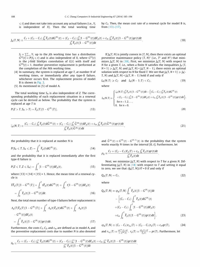
JBðT;NÞ �CT þ ðCY � CTÞ

R T0 FpðtÞdGðNÞðtÞ þ ðCZ � CTÞ

R T0 ½1� GðNÞðtÞ�dFpðtÞ þ cm

R T0 FpðtÞ½1� GðNÞðtÞ�qrðtÞdtR T

0 FpðtÞ½1� GðNÞðtÞ�dt: ð18Þ

Sj �Pj

i¼1 Yi up to the jth working time has a distributionG(j)(t) � P(Sj 6 t) and is also independent of X, where G(j)(t)is the j-fold Stieltjes convolution of G(t) with itself andG(0)(t) � 1. Another preventive replacement is performed atthe completion of the Nth working time.

(4) In summary, the system is replaced at age T, at number N ofworking times, or immediately after any type-II failure,whichever occurs first. The replacement process of modelB is shown in Fig. 2.

(5) As mentioned in (5) of model A.

The total working time SN is also independent of Z. The corre-sponding probability of each replacement situation in a renewalcycle can be derived as below. The probability that the system isreplaced at age T is

PðZ > T; SN > TÞ ¼ FpðTÞ½1� GðNÞðTÞ�; ð13Þ

fBðN; TÞ �ðCT � CY Þ

R T0 FpðtÞdeGðNÞðtÞ þ ðCZ � CTÞ

R T0eGðNÞðtÞdFpðtÞ þ cm

R T0 FpðtÞeGðNÞðtÞqrðtÞdtR T

0 FpðtÞeGðNÞðtÞdt; ð21Þ

the probability that it is replaced at number N is

PðSN 6 T; SN 6 ZÞ ¼Z T

0FpðtÞdGðNÞðtÞ; ð14Þ

and the probability that it is replaced immediately after the firsttype-II failure is

PðZ 6 T; Z 6 SNÞ ¼Z T

0½1� GðNÞðtÞ�dFpðtÞ; ð15Þ

where (13) + (14) + (15) = 1. Hence, the mean time of a renewal cy-cle is

TFpðTÞ½1� GðNÞðTÞ� þZ T

0tFpðtÞdGðNÞðtÞ þ

Z T

0t½1� GðNÞðtÞ�dFpðtÞ

¼Z T

0FpðtÞ½1� GðNÞðtÞ�dt: ð16Þ

Next, the total mean number of type-I failures before replacement is

KqðTÞFpðTÞ½1� GðNÞðTÞ� þZ T

0KqðtÞFpðtÞdGðNÞðtÞ þ

Z T

0KqðtÞ½1

� GðNÞðtÞ�dFpðtÞ

¼Z T

0FpðtÞ½1� GðNÞðtÞ�qrðtÞdt: ð17Þ

Furthermore, the costs CT, CZ, and cm are defined as in model A, andthe preventive replacement costs due to number N is also denoted

hB �CT þ ðCY � CTÞ

R10 FpðtÞdGðNÞðtÞ þ ðCZ � CTÞ

R10 ½1� GðNÞðtÞdFpðtÞ þ cR1

0 FpðtÞ½1� GðNÞðtÞ�dt

by CY. Then, the mean cost rate of a renewal cycle for model B is,from (13)–(17),

If JB(T, N) is jointly convex in (T, N), then there exists an optimalpreventive maintenance policy (T, N)⁄ (i.e., T⁄ and N⁄) that mini-mizes JB(T, N) in (18). First, we minimize JB(T, N) with respect toN for a given T, i.e., when a finite N satisfies the inequalities JB (T,N + 1) P JB(T, N) and JB(T, N) < JB(T, N � 1), there exists an optimalsolution with respect to N for fixed T. We see that JB(T, N + 1) P JB(-T, N) and JB(T, N) < JB(T, N � 1) hold if and only if

LBðN; TÞP CT and LBðN � 1; TÞ < CT ; ð19Þ

where

LBðN;TÞ �

fBðN;TÞR T

0 FpðtÞ½1�GðNÞðtÞ�dt� ðCY �CT ÞR T

0 FpðtÞdGðNÞðtÞn

þðCZ�CT ÞR T

0 ½1�GðNÞðtÞ�dFpðtÞþcmR T

0 FpðtÞ½1�GðNÞðtÞ�qrðtÞdto;

for n¼1;2; . . . ;0; for n¼0;

8>>>>><>>>>>:ð20Þ

and eGðNÞðtÞ � GðNÞðtÞ � GðNþ1ÞðtÞ is the probability that the systemworks exactly N times in the interval [0, t]. Furthermore, let

qB �CT þ ðCZ � CTÞFpðTÞ þ cm

R T0 FpðtÞqrðtÞdtR T

0 FpðtÞdt:

Next, we minimize JB(T, N) with respect to T for a given N. Dif-ferentiating JB(T, N) in (18) with respect to T and setting it equalto zero, we see that @JB(T, N)/@T = 0 if and only if

QBðT; NÞ ¼ CT ; ð22Þ

where

QBðT; NÞ � uBðT; NÞZ T

0FpðtÞ½1� GðNÞðtÞ�dt

� ðCY � CTÞZ T

0FpðtÞdGðNÞðtÞ

�þðCZ � CTÞ

Z T

0½1� GðNÞðtÞ�dFpðtÞ

þcm

Z T

0FpðtÞ½1� GðNÞðtÞ�qrðtÞdt

�; ð23Þ

uBðT; NÞ � ðCY � CTÞrGN ðTÞ þ ðCZ � CTÞrpðTÞ þ cmqrðTÞ; ð24Þ

and rGN ðTÞ �@GðNÞðTÞ=@T1�GðNÞðTÞ

; rpðTÞ � @FpðTÞ=@T

FpðTÞ¼ prðTÞ. Furthermore, let

mR1

0 FpðtÞ½1� GðNÞðtÞ�qrðtÞdt:

C.-C. Chang / Computers & Industrial Engineering 67 (2014) 185–194 189

Now, the optimal preventive maintenance policy (T, N)⁄ thatminimizes the mean cost rate JB(T, N) can be summarized as below.

JBðNÞ � limT!1

JBðT;NÞ ¼CYR1

0 FpðtÞdGðNÞðtÞ þ CZR1

0 ½1� GðNÞðtÞ�dFpðtÞ þ cmR1

0 FpðtÞ½1� GðNÞðtÞ�qrðtÞdtR10 FpðtÞ½1� GðNÞðtÞ�dt

: ð28Þ

Theorem 2. Suppose that fB(N; T) is increasing with N and uB (T; N)is continuous and increasing with T. If limN?1 fB(N; T) > qB andlimT?1 uB (T; N) > hB, then the system is replaced at age T, at numberN of working times, or immediately after any type-II failure, whicheveroccurs first, and N⁄ is a unique solution of (19), and T⁄ is a finite andunique solution of (22).

Proof. See Appendix B. h

Remark 2. uB(T; N) can be regarded as the expected marginal costof this policy at age T as stated in Remark 1. The fB(N; T) can beinterpreted as the expected marginal cost of this policy at numberN of working times. Then the condition (19) is equivalent to

fBðN; TÞP JBðT;NÞ and fBðN � 1; TÞ < JBðT;N � 1Þ:The optimum N (i.e., N⁄; minN JB(T, N) = JB (T, N⁄)) must satisfy

the equivalent condition that indicates it is worthy to increasethe prefixed number of working times (N) if fB(N; T) < JB(T, N). Sup-posing that CZ > CT = CY, r(t) increases strictly and G(t) = 1 � e�ht, i.e.,GðNÞðtÞ ¼ 1�

PN�1j¼0 ½ðhtÞj=j!�e�ht , the expected marginal cost in (21)

can be rewritten as

fBðN; TÞ ¼ðCZ � CTÞ

R T0 ðhtÞNe�htdFpðtÞ þ cm

R T0 ðhtÞNe�htFpðtÞqrðtÞdtR T

0 ðhtÞNe�htFpðtÞdt;

which is increasing with N sinceR T

0 ðhtÞNe�htdFpðtÞ=R T

0 ðhtÞNe�htFp

ðtÞdt increases (Nakagawa, 2005, p. 86) andR T

0 ðhtÞNe�htFpðtÞqrðtÞdt=

R T0 ðhtÞNe�htFpðtÞdt increases with N (using the method of

Lemma 1 in Chang et al. (2011)).In particular, when N = 1, JB(T,1) agrees with (7). We also dem-

onstrate that several previous models are special cases of model B.

� Case B1. q = 0. This case is considered by Chen, Mizutani, andNakagawa (2010), in which the system is replaced at time T,number N or at complete failure, whichever occurs first. If weset q = 0 in (18), then the mean cost rate is

JB1ðT;NÞ�CT þðCY �CTÞ

R T0 FðtÞdGðNÞðtÞþðCZ�CTÞ

R T0 ½1�GðNÞðtÞ�dFðtÞR T

0 FðtÞ½1�GðNÞðtÞ�dt:

ð25Þ

� Case B2. q = 1. This case is considered by Chen, Nakamura, andNakagawa (2010), in which the system is replaced at time T ornumber N, and undergoes minimal repair at complete failure. Ifwe set q = 1 in (18), then the mean cost rate is

JB2ðT;NÞ �CT þ ðCY � CTÞGðNÞðTÞ þ cm

R T0 ½1� GðNÞðtÞ�rðtÞdtR T

0 ½1� GðNÞðtÞ�dt:

ð26Þ

Y1 YN

T

Y1 Yj

T

Y1 Yj

T

� Case B3. N ?1. When the system is replaced at time T or at thefirst type-II failure, whichever occurs first, the mean cost ratebecomes

Preventive replacement at the first working time completionover age or number of random timesCorrective replacement at type-II failure

Fig. 3. Process of preventive and corrective replacement in Model C.

JBðTÞ � limN!1

JBðT;NÞ

¼CT þ ðCZ � CTÞFpðTÞ þ cm

R T0 FpðtÞqrðtÞdtR T

0 FpðtÞdt: ð27Þ

� Case B4. T ?1. When the system is replaced at number N ofworking times or at the first type-II failure, whichever occursfirst, the mean cost rate becomes

2.3. Model C

This model assumes another extended preventive maintenancepolicy over age T for a system in which repair, maintenance, andreplacement take place according to the following scheme.

(1) As mentioned in (1) of model A, but a preventive replace-ment is planned to carry out at the first completion of work-ing time over age T.

(2) and (3) As mentioned in (2) and (3) of model B.(4) In summary, the system is replaced at the first completion of

working time over age T, at the Nth completion of workingtimes, or immediately after any type-II failure, whicheveroccurs first. The replacement process of model C is shownin Fig. 3.

(5) As mentioned in (5) of model A.

The corresponding probability of each replacement situation ina renewal cycle can be derived as below. The probability that thesystem is replaced at the first completion of working time overage T is

PT �XN�1

j¼0

Z T

0

Z 1

T�tFpðt þ uÞdGðuÞ

� �dGðjÞðtÞ; ð29Þ

the probability that it is replaced at number N is

PY �Z T

0FpðtÞdGðNÞðtÞ; ð30Þ

and the probability that it is replaced immediately after the firsttype-II failure is

PZ �XN�1

j¼0

Z T

0½GðjÞðtÞ � Gðjþ1ÞðtÞ�dFpðtÞ

þXN�1

j¼0

Z T

0

Z 1

T�t½Fpðt þ uÞ � FpðTÞ�dGðuÞ

� �dGðjÞðtÞ

¼Z T

0½1� GðNÞðtÞ�dFpðtÞ

þXN�1

j¼0

Z T

0

Z 1

T�t½Fpðt þ uÞ � FpðTÞ�dGðuÞ

� �dGðjÞðtÞ; ð31Þ

where (29) + (30) + (31) = 1. Hence, the mean time of a renewalcycle is

190 C.-C. Chang / Computers & Industrial Engineering 67 (2014) 185–194

XN�1

j¼0

Z T

0

Z 1

T�tðt þ uÞFpðt þ uÞdGðuÞ

� �dGðjÞðtÞ

þZ T

0tFpðtÞdGðNÞðtÞ þ

Z T

0t½1� GðNÞðtÞ�dFpðtÞ

þXN�1

j¼0

Z T

0

Z 1

T�t

Z tþu

TvdFpðvÞ

� �dGðuÞ

� �dGðjÞðtÞ

¼Z T

0½1� GðNÞðtÞ�FpðtÞdt

þXN�1

j¼0

Z T

0

Z 1

TGðu� tÞFpðuÞdu

� �dGðjÞðtÞ: ð32Þ

Next, the total mean number of type-I failures before replace-ment is

XN�1

j¼0

Z T

0

Z 1

T�tKqðt þ uÞFpðt þ uÞdGðuÞ

� �dGðjÞðtÞ

þZ T

0KqðtÞFpðtÞdGðNÞðtÞ þ

Z T

0KqðtÞ½1� GðNÞðtÞ�dFpðtÞ

þXN�1

j¼0

Z T

0

Z 1

T�t

Z tþu

TKqðvÞdFpðvÞ

� �dGðuÞ

� �dGðjÞðtÞ

¼Z T

0½1� GðNÞðtÞ�FpðtÞqrðtÞdt

þXN�1

j¼0

Z T

0

Z 1

TGðu� tÞFpðuÞqrðuÞdu

� �dGðjÞðtÞ: ð33Þ

Furthermore, the costs, CY, CZ, and cm are defined as in model B, andthe preventive replacement costs due to the first completion ofworking time over age T is also denoted by CT. Then, the mean costrate of a renewal cycle for model C is, from (29)–(33),

JCðT;NÞ �CZ þ ðCT � CZÞPT þ ðCY � CZÞPY þ cm

R T0 ½1� GðNÞðtÞ�FpðtÞqrðtÞdt þ

PN�1j¼0

R T0

R1T Gðu� tÞFpðuÞqrðuÞdu

h idGðjÞðtÞ

n oR T

0 ½1� GðNÞðtÞ�FpðtÞdt þPN�1

j¼0

R T0

R1T Gðu� tÞFpðuÞdu

h idGðjÞðtÞ

: ð34Þ

Note that if N ?1, this corresponds to the preventive mainte-nance model where the system is replaced at the first completionof working time over age T or immediately after the first type-IIfailure, whichever occurs first. The mean cost rate is, from (34),

JCðTÞ � limN!1

JCðT;NÞ

¼CZ þ ðCT � CZÞ

R1T FpðtÞdGðtÞ þ

R T0

R1T�t Fpðt þ uÞdGðuÞ

� �dMGðtÞ

n oþ cm

R T0 FpðtÞqrðtÞdt þ

R1T GðtÞFpðtÞqrðtÞdt þ

R T0

R1T Gðu� tÞFpðuÞqrðuÞdu

h idMGðtÞ

n oR T

0 FpðtÞdt þR1

T GðtÞFpðtÞdt þR T

0

R1T Gðu� tÞFpðuÞdu

h idMGðtÞ

;

ð35Þ

where MGðtÞ �P1

j¼1 GðjÞðtÞ. Now, if JC(T) is convex in T, then thereexists an optimal policy T⁄ that minimizes JC(T) in (35) and satisfies@JC(T)/@T = 0. We have that @JC(T)/@T = 0 if and only if

Q CðTÞ ¼ CT ; ð36Þ

where

QCðTÞ � uCðTÞZ T

0FpðtÞdt þ

Z 1

TGðtÞFpðtÞdt

�þZ T

0

Z 1

TGðu� tÞFpðuÞdu

� �dMGðtÞ

�� ðCT � CZÞ �1þ

Z 1

TFpðtÞdGðtÞ

�þZ T

0

Z 1

T�tFpðt þ uÞdGðuÞ

� �dMGðtÞ

�� cm

Z T

0FpðtÞqrðtÞdt þ

Z 1

TGðtÞFpðtÞqrðtÞdt

�þZ T

0

Z 1

TGðu� tÞFpðuÞqrðuÞdu

� �dMGðtÞ

�; ð37Þ

uCðTÞ�ðCZ�CTÞ

R10 FpðTÞ�FpðTþ tÞ� �

dGðtÞþ cmR1

0 GðtÞFpðTþ tÞqrðTþ tÞdtR10 GðtÞFpðTþ tÞdt

:

ð38Þ

Furthermore, let hC � CZ þ cmR1

0 FpðtÞqrðtÞdt�

=R1

0 FpðtÞdt, we cansummarize the structure properties of the optimal policy T⁄ asfollows.

Theorem 3. Suppose that uC(T) is continuous and increasing with T.If limT?1 uC(T) > hC, then there exists a finite and unique T⁄ whichsatisfies (36) and the optimal mean cost rate is JC(T⁄) = uC(T⁄);otherwise, the optimal policy is T⁄?1.

Proof. See Appendix C. h

Next, if T ?1, this corresponds to the preventive maintenancemodel where at the Nth completion of working times, or immedi-ately after the first type-II failure, whichever occurs first. The meancost rate is, from (34),

JCðNÞ� limT!1

JCðT;NÞ

¼CZþðCY �CZÞ

R10 FpðtÞdGðNÞðtÞþ cm

R10 ½1�GðNÞðtÞ�FpðtÞqrðtÞdtR1

0 ½1�GðNÞðtÞ�FpðtÞdt:

ð39Þ

Now, If JC(N) is convex in N, then there exists an optimal policy N⁄

that minimizes JC(N) in (39) and satisfies JC(N + 1) P JC(N) andJC(N) < JC(N � 1).

We see that JC(N + 1) P JC(N) and JC(N) < JC(N � 1) hold if andonly if

LCðNÞP CZ and LCðN � 1Þ < CZ ; ð40Þ

C.-C. Chang / Computers & Industrial Engineering 67 (2014) 185–194 191

where

LCðNÞ �

fCðNÞR1

0 ½1� GðNÞðtÞ�FpðtÞdt

�ðCY � CZÞR1

0 FpðtÞdGðNÞðtÞþcm

R10 ½1� GðNÞðtÞ�FpðtÞqrðtÞdt; for n ¼ 1;2; . . . ;

0; for n ¼ 0;

8>>>><>>>>:ð41Þ

fCðNÞ �ðCZ � CYÞ

R10 FpðtÞdeGðNÞðtÞ þ cm

R10eGðNÞðtÞFpðtÞqrðtÞdtR1

0eGðNÞðtÞFpðtÞdt

;

ð42Þ

and eGðNÞðtÞ � GðNÞðtÞ � GðNþ1ÞðtÞ.

JC1ðT;NÞ �CZ þ ðCT � CZÞ

PN�1j¼0

R T0

R1T�t Fðt þ uÞdGðuÞ

� �dGðjÞðtÞ þ ðCY � CTÞ

R T0 FðtÞdGðNÞðtÞR T

0 ½1� GðNÞðtÞ�FðtÞdt þPN�1

j¼0

R T0

R1T Gðu� tÞFðuÞdu

h idGðjÞðtÞ

: ð43Þ

Furthermore, let qC �CZþcm

R10

FpðtÞqrðtÞdtR10

FpðtÞdt, the optimal policy N⁄ that

minimizes the mean cost rate JC(N) can be summarized as below.

Theorem 4. If fC(N) is increasing with N and limN?1 fC(N) > qC, thenthere exists a finite and unique N⁄ that satisfies LC(N⁄) P CZ and LC

(N⁄ � 1) < CZ for N⁄ = 1,2, . . . .

JC2ðT;NÞ �CT þ ðCY � CTÞGðNÞðTÞ þ cm

R T0 ½1� GðNÞðtÞ�rðtÞdt þ

PN�1j¼0

R T0

R1T Gðu� tÞrðuÞdu

h idGðjÞðtÞ

n oR T

0 ½1� GðNÞðtÞ�dt þPN�1

j¼0

R T0

R1T Gðu� tÞdu

h idGðjÞðtÞ

: ð44Þ

Proof. See Appendix D. h

Remark 3. uC(T) and fC(N) can be regarded as the expected mar-ginal cost of this policy at age T and the Nth completion of workingtimes as stated in Remarks 1 and 2, respectively. First, supposingthat CZ > CT, r(t) increases strictly, and G(t) = 1 � e�ht, the expectedmarginal cost in (38) can be rewritten as

uCðTÞ ¼ðCZ � CTÞ

R10 he�ht FpðTÞ � FpðT þ tÞ

� �dt þ cm

R10 e�htFpðT þ tÞqrðT þ tÞdtR1

0 e�htFpðT þ tÞdt

¼ ðCZ � CTÞFpðTÞR1

0 e�htFpðT þ tÞdt� h

" #þ cm

R10 e�htFpðT þ tÞqrðT þ tÞdtR1

0 e�htFpðT þ tÞdt;

which is also strictly increasing with T. When r(t) increases, it is notdifficult to show Fpðt þ TÞ=FpðTÞ decreases with T, henceFpðTÞ=

R10 e�htFpðT þ tÞdt increases with T. Next, supposing that

CZ > CY, r(t) increases strictly, and G(t) = 1 � e�ht, i.e.,

GðNÞðtÞ ¼ 1�PN�1

j¼0 ½ðhtÞj=j!�e�ht , the expected marginal cost in (42)can be rewritten as

fCðNÞ ¼ðCZ � CYÞ

R10 ðhtÞNe�htdFpðtÞ þ cm

R10 ðhtÞNe�htFpðtÞqrðtÞdtR1

0 ðhtÞNe�htFpðtÞdt;

which is increasing with N as explained in Remark 2.

If JC(T, N) is jointly convex in (T, N), then there exists a bivariateoptimal policy (T, N)⁄ (i.e., T⁄ and N⁄) that minimizes JC(T, N) in (34).In general, an explicit analytical express can be obtained using amethod similar to that in Model B. The optimal bivariate policy willbe computed numerically.

In particular, some special cases of model C can be demon-strated as below.

� Case C1. q = 0. This case is considered by Chen, Mizutani, andNakagawa (2010), in which the system is replaced at the firstcompletion of working time over age T, at the Nth completionof working times, or at complete failure, whichever occurs first.If we set q = 0 in (34), then the mean cost rate is

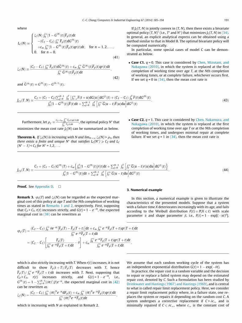
� Case C2. q = 1. This case is considered by Chen, Nakamura, andNakagawa (2010), in which the system is replaced at the firstcompletion of working time over age T or at the Nth completionof working times, and undergoes minimal repair at completefailure. If we set q = 1 in (34), then the mean cost rate is

3. Numerical example

In this section, a numerical example is given to illustrate thecharacteristics of the presented models. Suppose that a systemwith a failure time X deteriorates increasingly with its age, and failsaccording to the Weibull distribution F(t) � P(X 6 t) with scaleparameter a and shape parameter b, i.e., F(t) = 1 � exp[(�at)b].

We assume that each random working cycle of the system hasan independent exponential distribution G(t) = 1 � exp(�ht).

In practice, the repair cost is a random variable and the decisionto repair or replace a failed system may depend on the estimatedrepair cost, denoted by C. Such a formulation has been studied byDrinkwater and Hastings (1967) and Hastings (1969), and is centralto what is called repair limit replacement policy. Here, we considera repair limit replacement policy where, in a failure state, one re-places the system or repairs it depending on the random cost C. Asystem undergoes a corrective replacement if C > dc1 and isminimally repaired if C 6 dc1, where c1 is the constant cost of

192 C.-C. Chang / Computers & Industrial Engineering 67 (2014) 185–194

replacement at failure and d (0 6 d 6 1) can be interpreted as a frac-tion of the constant cost c1. Suppose that the random repair cost Chas a distribution L(u) and density function l(u), with mean l andstandard deviation r. Hence, d satisfies q ¼

R dc10 lðuÞdu, and the ex-

pected minimal repair cost cm can be given by cm ¼ 1q

R dc10 ulðuÞdu.

The parameter q (minimal repair probability) is varied to determineits influence on the optimal policies. We assume that it is a param-eter known to the decision maker. For instance, we all have to makesuch decisions once in a while, such as repairing or replacing a com-puter, a car, or a refrigerator, depending on the maintenance cost,and in each case we have our own q.

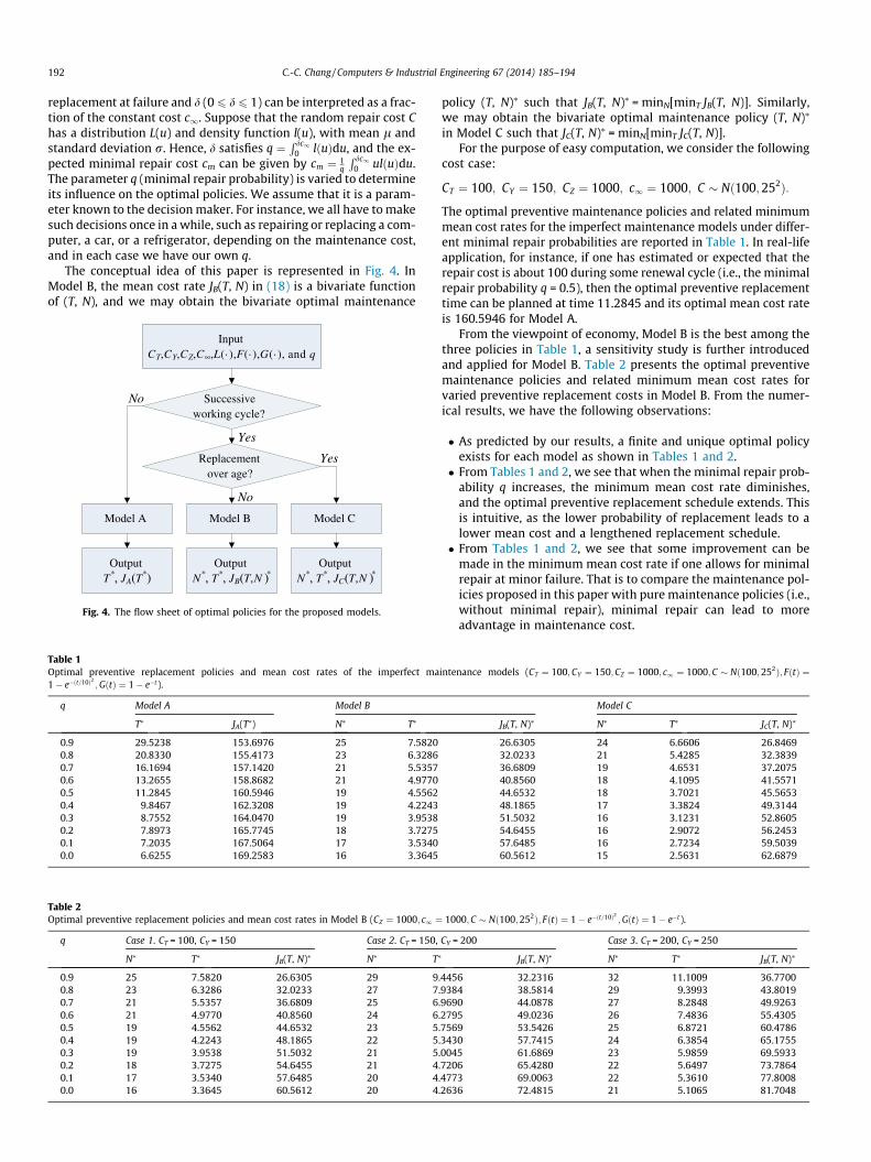
The conceptual idea of this paper is represented in Fig. 4. InModel B, the mean cost rate JB(T, N) in (18) is a bivariate functionof (T, N), and we may obtain the bivariate optimal maintenance

Table 1Optimal preventive replacement policies and mean cost rates of the imperfect ma1� e�ðt=10Þ2 ;GðtÞ ¼ 1� e�t).

q Model A Model B

T⁄ JA(T⁄) N⁄ T⁄

0.9 29.5238 153.6976 25 7.58200.8 20.8330 155.4173 23 6.32860.7 16.1694 157.1420 21 5.53570.6 13.2655 158.8682 21 4.97700.5 11.2845 160.5946 19 4.55620.4 9.8467 162.3208 19 4.22430.3 8.7552 164.0470 19 3.95380.2 7.8973 165.7745 18 3.72750.1 7.2035 167.5064 17 3.53400.0 6.6255 169.2583 16 3.3645

InputCT,CY,CZ,C ,L(· ),F(· ),G(· ), and q

Successiveworking cycle?

Replacementover age?

Model BModel A Model C

Yes

No

No

Yes

OutputN*, T*, JC(T,N )*

OutputN*, T*, JB(T,N )*

OutputT*, JA(T*)

Fig. 4. The flow sheet of optimal policies for the proposed models.

Table 2Optimal preventive replacement policies and mean cost rates in Model B (CZ ¼ 1000; c1 ¼

q Case 1. CT = 100, CY = 150 Case 2. CT = 150,

N⁄ T⁄ JB(T, N)⁄ N⁄ T⁄

0.9 25 7.5820 26.6305 29 90.8 23 6.3286 32.0233 27 70.7 21 5.5357 36.6809 25 60.6 21 4.9770 40.8560 24 60.5 19 4.5562 44.6532 23 50.4 19 4.2243 48.1865 22 50.3 19 3.9538 51.5032 21 50.2 18 3.7275 54.6455 21 40.1 17 3.5340 57.6485 20 40.0 16 3.3645 60.5612 20 4

policy (T, N)⁄ such that JB(T, N)⁄ = minN[minT JB(T, N)]. Similarly,we may obtain the bivariate optimal maintenance policy (T, N)⁄

in Model C such that JC(T, N)⁄ = minN[minT JC(T, N)].For the purpose of easy computation, we consider the following

cost case:

CT ¼ 100; CY ¼ 150; CZ ¼ 1000; c1 ¼ 1000; C � Nð100;252Þ:

The optimal preventive maintenance policies and related minimummean cost rates for the imperfect maintenance models under differ-ent minimal repair probabilities are reported in Table 1. In real-lifeapplication, for instance, if one has estimated or expected that therepair cost is about 100 during some renewal cycle (i.e., the minimalrepair probability q = 0.5), then the optimal preventive replacementtime can be planned at time 11.2845 and its optimal mean cost rateis 160.5946 for Model A.

From the viewpoint of economy, Model B is the best among thethree policies in Table 1, a sensitivity study is further introducedand applied for Model B. Table 2 presents the optimal preventivemaintenance policies and related minimum mean cost rates forvaried preventive replacement costs in Model B. From the numer-ical results, we have the following observations:

� As predicted by our results, a finite and unique optimal policyexists for each model as shown in Tables 1 and 2.� From Tables 1 and 2, we see that when the minimal repair prob-

ability q increases, the minimum mean cost rate diminishes,and the optimal preventive replacement schedule extends. Thisis intuitive, as the lower probability of replacement leads to alower mean cost and a lengthened replacement schedule.� From Tables 1 and 2, we see that some improvement can be

made in the minimum mean cost rate if one allows for minimalrepair at minor failure. That is to compare the maintenance pol-icies proposed in this paper with pure maintenance policies (i.e.,without minimal repair), minimal repair can lead to moreadvantage in maintenance cost.

intenance models (CT ¼ 100; CY ¼ 150;CZ ¼ 1000; c1 ¼ 1000;C � Nð100;252Þ; FðtÞ ¼

Model C

JB(T, N)⁄ N⁄ T⁄ JC(T, N)⁄

26.6305 24 6.6606 26.846932.0233 21 5.4285 32.383936.6809 19 4.6531 37.207540.8560 18 4.1095 41.557144.6532 18 3.7021 45.565348.1865 17 3.3824 49.314451.5032 16 3.1231 52.860554.6455 16 2.9072 56.245357.6485 16 2.7234 59.503960.5612 15 2.5631 62.6879

1000;C � Nð100;252Þ; FðtÞ ¼ 1� e�ðt=10Þ2 ;GðtÞ ¼ 1� e�t).

CY = 200 Case 3. CT = 200, CY = 250

JB(T, N)⁄ N⁄ T⁄ JB(T, N)⁄

.4456 32.2316 32 11.1009 36.7700

.9384 38.5814 29 9.3993 43.8019

.9690 44.0878 27 8.2848 49.9263

.2795 49.0236 26 7.4836 55.4305

.7569 53.5426 25 6.8721 60.4786

.3430 57.7415 24 6.3854 65.1755

.0045 61.6869 23 5.9859 69.5933

.7206 65.4280 22 5.6497 73.7864

.4773 69.0063 22 5.3610 77.8008

.2636 72.4815 21 5.1065 81.7048

C.-C. Chang / Computers & Industrial Engineering 67 (2014) 185–194 193

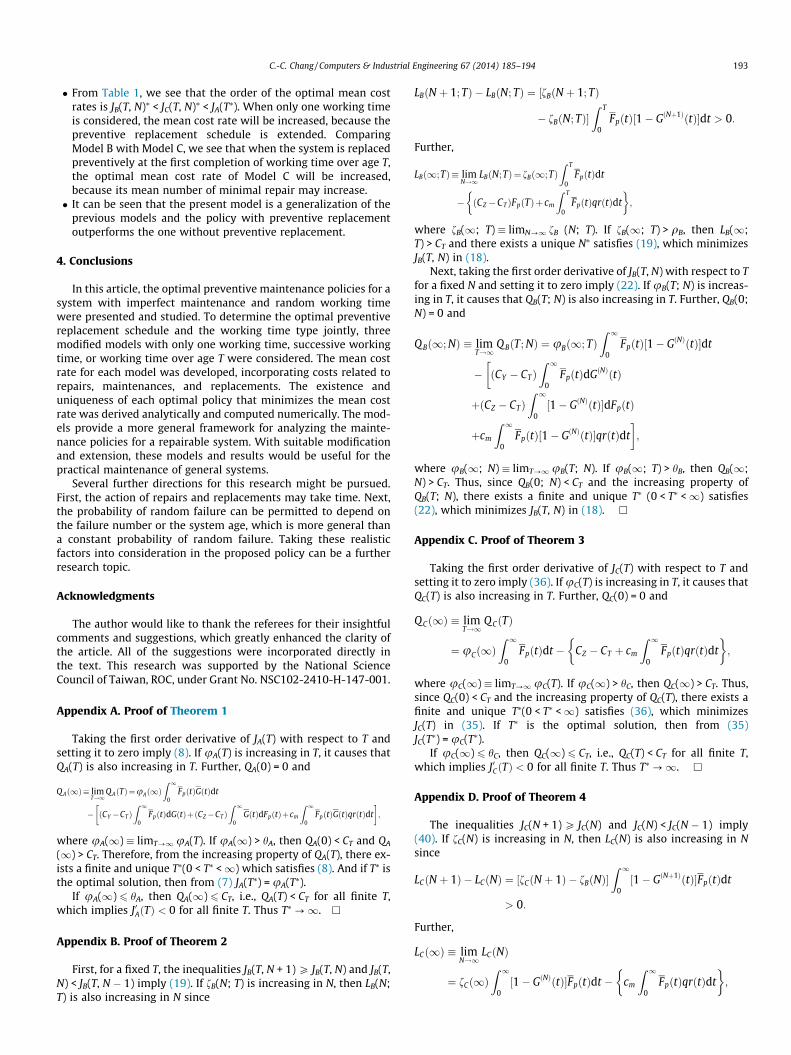
� From Table 1, we see that the order of the optimal mean costrates is JB(T, N)⁄ < JC(T, N)⁄ < JA(T⁄). When only one working timeis considered, the mean cost rate will be increased, because thepreventive replacement schedule is extended. ComparingModel B with Model C, we see that when the system is replacedpreventively at the first completion of working time over age T,the optimal mean cost rate of Model C will be increased,because its mean number of minimal repair may increase.� It can be seen that the present model is a generalization of the

previous models and the policy with preventive replacementoutperforms the one without preventive replacement.

4. Conclusions

In this article, the optimal preventive maintenance policies for asystem with imperfect maintenance and random working timewere presented and studied. To determine the optimal preventivereplacement schedule and the working time type jointly, threemodified models with only one working time, successive workingtime, or working time over age T were considered. The mean costrate for each model was developed, incorporating costs related torepairs, maintenances, and replacements. The existence anduniqueness of each optimal policy that minimizes the mean costrate was derived analytically and computed numerically. The mod-els provide a more general framework for analyzing the mainte-nance policies for a repairable system. With suitable modificationand extension, these models and results would be useful for thepractical maintenance of general systems.

Several further directions for this research might be pursued.First, the action of repairs and replacements may take time. Next,the probability of random failure can be permitted to depend onthe failure number or the system age, which is more general thana constant probability of random failure. Taking these realisticfactors into consideration in the proposed policy can be a furtherresearch topic.

Acknowledgments

The author would like to thank the referees for their insightfulcomments and suggestions, which greatly enhanced the clarity ofthe article. All of the suggestions were incorporated directly inthe text. This research was supported by the National ScienceCouncil of Taiwan, ROC, under Grant No. NSC102-2410-H-147-001.

Appendix A. Proof of Theorem 1

Taking the first order derivative of JA(T) with respect to T andsetting it to zero imply (8). If uA(T) is increasing in T, it causes thatQA(T) is also increasing in T. Further, QA(0) = 0 and

QAð1Þ� limT!1

QAðTÞ¼uAð1ÞZ 1

0FpðtÞGðtÞdt

� ðCY �CT ÞZ 1

0FpðtÞdGðtÞþðCZ�CT Þ

Z 1

0GðtÞdFpðtÞþcm

Z 1

0FpðtÞGðtÞqrðtÞdt

� �;

where uA(1) � limT?1 uA(T). If uA(1) > hA, then QA(0) < CT and QA

(1) > CT. Therefore, from the increasing property of QA(T), there ex-ists a finite and unique T⁄(0 < T⁄ <1) which satisfies (8). And if T⁄ isthe optimal solution, then from (7) JA(T⁄) = uA(T⁄).

If uA(1) 6 hA, then QA(1) 6 CT, i.e., QA(T) < CT for all finite T,which implies J0AðTÞ < 0 for all finite T. Thus T⁄?1. h

Appendix B. Proof of Theorem 2

First, for a fixed T, the inequalities JB(T, N + 1) P JB(T, N) and JB(T,N) < JB(T, N � 1) imply (19). If fB(N; T) is increasing in N, then LB(N;T) is also increasing in N since

LBðN þ 1; TÞ � LBðN; TÞ ¼ ½fBðN þ 1; TÞ

� fBðN; TÞ�Z T

0FpðtÞ½1� GðNþ1ÞðtÞ�dt > 0:

Further,

LBð1;TÞ� limN!1

LBðN;TÞ¼ fBð1;TÞZ T

0FpðtÞdt

� ðCZ�CTÞFpðTÞþ cm

Z T

0FpðtÞqrðtÞdt

� �;

where fB(1; T) � limN?1 fB (N; T). If fB(1; T) > qB, then LB(1;T) > CT and there exists a unique N⁄ satisfies (19), which minimizesJB(T, N) in (18).

Next, taking the first order derivative of JB(T, N) with respect to Tfor a fixed N and setting it to zero imply (22). If uB(T; N) is increas-ing in T, it causes that QB(T; N) is also increasing in T. Further, QB(0;N) = 0 and

QBð1; NÞ � limT!1

Q BðT; NÞ ¼ uBð1; TÞZ 1

0FpðtÞ½1� GðNÞðtÞ�dt

� ðCY � CTÞZ 1

0FpðtÞdGðNÞðtÞ

�þðCZ � CTÞ

Z 1

0½1� GðNÞðtÞ�dFpðtÞ

þcm

Z 1

0FpðtÞ½1� GðNÞðtÞ�qrðtÞdt

�;

where uB(1; N) � limT?1 uB(T; N). If uB(1; T) > hB, then QB(1;N) > CT. Thus, since QB(0; N) < CT and the increasing property ofQB(T; N), there exists a finite and unique T⁄ (0 < T⁄ <1) satisfies(22), which minimizes JB(T, N) in (18). h

Appendix C. Proof of Theorem 3

Taking the first order derivative of JC(T) with respect to T andsetting it to zero imply (36). If uC(T) is increasing in T, it causes thatQC(T) is also increasing in T. Further, QC(0) = 0 and

QCð1Þ � limT!1

Q CðTÞ

¼ uCð1ÞZ 1

0FpðtÞdt � CZ � CT þ cm

Z 1

0FpðtÞqrðtÞdt

� �;

where uC(1) � limT?1 uC(T). If uC(1) > hC, then QC(1) > CT. Thus,since QC(0) < CT and the increasing property of QC(T), there exists afinite and unique T⁄(0 < T⁄ <1) satisfies (36), which minimizesJC(T) in (35). If T⁄ is the optimal solution, then from (35)JC(T⁄) = uC(T⁄).

If uC(1) 6 hC, then QC(1) 6 CT, i.e., QC(T) < CT for all finite T,which implies J0CðTÞ < 0 for all finite T. Thus T⁄?1. h

Appendix D. Proof of Theorem 4

The inequalities JC(N + 1) P JC(N) and JC(N) < JC(N � 1) imply(40). If fC(N) is increasing in N, then LC(N) is also increasing in Nsince

LCðN þ 1Þ � LCðNÞ ¼ ½fCðN þ 1Þ � fBðNÞ�Z 1

0½1� GðNþ1ÞðtÞ�FpðtÞdt

> 0:

Further,

LCð1Þ � limN!1

LCðNÞ

¼ fCð1ÞZ 1

0½1� GðNÞðtÞ�FpðtÞdt � cm

Z 1

0FpðtÞqrðtÞdt

� �;

194 C.-C. Chang / Computers & Industrial Engineering 67 (2014) 185–194

where fC(1) � limN?1 fC(N). If fC(1) > qC, then LC(1) > CZ andthere exists a unique N⁄ satisfies (40), which minimizes JC(N) in(39). h

References

Barlow, R. E., & Hunter, L. C. (1960). Optimum preventive maintenance policies.Operations Research, 8, 90–100.

Beichelt, F. (1993). A unifying treatment of replacement policies with minimalrepair. Naval Research Logistics, 40, 51–67.

Berg, M., & Cléroux, R. (1982). A marginal cost analysis for an age replacementpolicy with minimal repair. INFOR, 20, 258–263.

Block, H. W., Broges, W., & Savits, T. H. (1985). Age-dependent minimal repair.Journal of Applied Probability, 22, 370–386.

Brown, M., & Proschan, F. (1965). Mathematical theory of reliability. New York: JohnWiley & Sons.

Brown, M., & Proschan, F. (1983). Imperfect repair. Journal of Applied Probability, 20,851–859.

Chang, C. C., Sheu, S. H., & Chen, Y. L. (2010). Optimal number of minimal repairsbefore replacement based on a cumulative repair-cost limit policy. Computersand Industrial Engineering, 59, 603–610.

Chang, C. C., Sheu, S. H., & Chen, Y. L. (2013a). A bivariate optimal replacementpolicy for a system with age-dependent minimal repair and cumulative repair-cost limit. Communications in Statistics – Theory and Methods, 42(22),4108–4126.

Chang, C. C., Sheu, S. H., & Chen, Y. L. (2013b). Optimal replacement model with age-dependent failure type based on a cumulative repair-cost limit. AppliedMathematical Modelling, 37, 308–317.

Chang, C. C., Sheu, S. H., Chen, Y. L., & Zhang, Z. G. (2011). A multi-criteria optimalreplacement policy for a system subject to shocks. Computers and IndustrialEngineering, 61, 1035–1043.

Chen, Y. L. (2012). A bivariate optimal imperfect preventive maintenance policy fora used system with two-type shocks. Computers and Industrial Engineering, 63,1227–1234.

Chen, M., Mizutani, S., & Nakagawa, T. (2010). Random and age replacementpolicies. International Journal of Reliability, Quality and Safety Engineering, 17(1),27–39.

Chen, M., Nakamura, S., & Nakagawa, T. (2010). Replacement and preventivemaintenance models with random working times. IEICE Transactions onFundamentals of Electronics, Communications and Computer Science, 500–507.

Drinkwater, R. W., & Hastings, N. A. J. (1967). A economic replacement model.Operational Research Quarterly, 18, 121–138.

Hastings, N. A. J. (1969). The repair limit replacement method. Operational ResearchQuarterly, 20, 337–349.

Huang, Y. S., Lin, Y. J., & Ho, J. W. (2013). A study on negative binomial inspection forimperfect production systems. Computers and Industrial Engineering, 65(4),605–613.

Kijima, M. (1989). Some results for repairable systems with general repair. Journal ofApplied Probability, 26, 89–102.

Kijima, M., Morimura, H., & Sujuki, Y. (1988). Periodical replacement problemwithout assuming minimal repair. European Journal of Operational Research, 37,194–203.

Kijima, M., & Nakagawa, T. (1991). Accumulative damage shock model withimperfect preventive maintenance. Naval Research Logistics, 38, 145–156.

Liu, Y., Huang, H. Z., & Wang, Z. (2013). A joint redundancy and imperfectmaintenance strategy optimization for multi-state systems. IEEE Transactions onReliability, 62(2), 368–378.

Nakagawa, T. (1988). Sequential imperfect preventive maintenance policies. IEEETransactions on Reliability, 37, 295–298.

Nakagawa, T. (2005). Maintenance theory of reliability. London: Springer.Nakagawa, T. (2008). Advanced reliability models and maintenance policies. London:

Springer.Pham, H., & Wang, H. (1996). Imperfect maintenance. European Journal of

Operational Research, 94, 425–438.Stadje, W. (2003). Renewal analysis of a replacement. Operations Research Letters,

31, 1–6.Sugiura, T., Mizutani, S., & Nakagawa, T. (2004). Optimal random replacement

policies. Tenth ISSAT International Conference on Reliability and Quality Design,99–103.

Xia, T., Xi, L., & Zhou, X. (2012). Modeling and optimizing maintenance schedule forenergy systems subject to degradation. Computers and Industrial Engineering,63(3), 607–614.

Xu, M., Chen, T., & Yang, X. (2012). Optimal replacement policy for safety-relatedmulti-component multi-state systems. Reliability Engineering and System Safety,99, 87–95.

Yun, W. Y., & Choi, C. H. (2000). Optimum replacement intervals with random timehorizon. Journal of Quality in Maintenance Engineering, 6, 269–274.

Zhao, X., Nakagawa, T., & Qian, C. (2012). Optimal imperfect preventivemaintenance policies for a used system. International Journal of SystemsScience, 43(9), 1632–1641.