Journal of Sound and Vibration (1995) 184(1), 35–58

ANALYSIS OF PERIODICALLY EXCITEDNON-LINEAR SYSTEMS BY A PARAMETRIC

CONTINUATION TECHNIQUE

C. P R. S

Acoustics and Dynamics Laboratory, Department of Mechanical Engineering,The Ohio State University, 206 West 18th Avenue, Columbus Ohio 43210-1107, U.S.A.

(Received 22 September 1993, and in final form 11 April 1994)

The dynamic behavior and frequency response of harmonically excited piecewise linearand/or non-linear systems has been the subject of several recent investigations. Most of theprior studies employed harmonic balance or Galerkin schemes, piecewise linear techniques,analog simulation and/or direct numerical integration (digital simulation). Such techniquesare somewhat limited in their ability to predict all of the dynamic characteristics, includingbifurcations leading to the occurrence of unstable, subharmonic, quasi-periodic and/orchaotic solutions. To overcome this problem, a parametric continuation scheme, based onthe shooting method, is applied specifically to a periodically excited piecewise linear/non-linear system, in order to improve understanding as well as to obtain the complete dynamicresponse. Parameter regions exhibiting bifurcations to harmonic, subharmonic or quasi-periodic solutions are obtained quite efficiently and systematically. Unlike other techniques,the proposed scheme can follow period-doubling bifurcations, and with some modificationsobtain stable quasi-periodic solutions and their bifurcations. This knowledge is essential inestablishing conditions for the occurrence of chaotic oscillations in any non-linear system.The method is first validated through the Duffing oscillator example, the solutions to whichare also obtained by conventional one-term harmonic balance and perturbation methods.The second example deals with a clearance non-linearity problem for both harmonic andperiodic excitations. Predictions from the proposed scheme match well with availableanalog simulation data as well as with multi-term harmonic balance results. Potentialsavings in computational time over direct numerical integration is demonstrated for someof the example cases. Also, this work has filled in some of the solution regimes for an impactpair, which were missed previously in the literature. Finally, one main limitation associatedwith the proposed procedure is discussed. 7 Academic Press Limited

1. INTRODUCTION

Piecewise linear or non-linear characteristics including clearances are found in manymachine elements and assemblies, such as gears, bearings, clutches, etc. Such non-linearsystems are often excited periodically while under the influence of a mean force or torque.The knowledge of steady state solutions, such as the frequency response characteristics,is essential from a dynamic design as well as a noise and vibration control viewpoint.Typical investigations have used one of the following solution techniques: (a) piecewise-linear techniques [1, 2], (b) harmonic balance methods [3–7], (c) analog simulation methods[8, 9] and (d) direct time-domain numerical integration [9–12]. Since non-linear systems,exhibit phenomena such as multiple solution regimes, subharmonic, and quasi-periodicand chaotic solutions, it is desirable to locate parameter regions in which such solutionsoccur in an efficient and unambiguous manner, which is the focus of this paper. Such ananalysis, for instance by using direct numerical integration, can only be accomplished by

35

0022–460X/95/260035+24 $12.00/0 7 1995 Academic Press Limited

. . 36

sweeping large initial condition maps. This procedure is obviously a rather laboriousprocess, especially when the dimension of the problem increases. The harmonic balanceschemes, which are usually variants of the Galerkin method [13], are also limited in theirability to track parameter bifurcations leading to the complex phenomena describedearlier, although a few attempts have been made towards that goal [3–6]. For instance,Comparin and Singh [7] could not explain some of the analog simulation results using theirdescribing function approximation [14].

Alternatively, computational techniques such as the shooting method [15–18] have beenused to locate the fixed points of Poincare maps (and hence the periodic solutions) andto determine their stability, as well as to obtain resonance backbone curves and otherdynamic characteristics very efficiently. Ling [15] has tested the shooting method for avariety of single- and two-degree-of-freedom non-linear systems, usually with cubicnon-linearities, and found the technique to be extremely useful. Sato et al. [18] applied thetechnique to map the tangent and pitchfork bifurcations in a gear pair with backlash anda periodic time-varying gear mesh-stiffness. The conventional shooting methods can beused to efficiently detect bifurcations, in conjunction with a parameter path followingtechnique [19–21], but previous investigations have limited their application to auto-nomous systems. Such a technique has yet to be widely applied to the analysis of externallyforced non-linear systems, especially those described earlier. Accordingly, the mainobjective of this paper, based on the literature reviewed above, is to adapt a parametriccontinuation (or path following) scheme, in conjunction with the shooting method, inorder specifically to study the dynamics of periodically forced piecewise non-linear systems.The proposed continuation procedure is first validated by applying it to a Duffingoscillator, and the results are compared with those reported in the literature, as well aswith predictions yielded by commonly used perturbation and one-term harmonic balanceschemes. Then, the proposed scheme is used to re-investigate the impact pair problem ofComparin and Singh [7]. An attempt is made to fill in some of the subharmonic solutionsand other regimes which were missed in their investigation. Both harmonic and periodicexcitations are considered and the various solution regimes are mapped completely.

2. POINT MAPPING FOR PERIODIC SOLUTIONS

2.1.

The general governing equation for a periodically forced (with fundamental excitationfrequency V) non-linear system with N degrees of freedom (DOF) can be written in statespace form, of dimension 2N, as follows (see Appendix A for the identification of symbols):

q'=F(q; Vt), (1)

where the state vector q is defined as

q=[q1 · · · q2N ]T, qi+1 = q'i , i=1, 3, . . . , 2N−1. (2, 3)

Here the q'i s and q'i+1s (i=1, 3, . . . , 2N−1) represent the displacements and velocities,respectively, of the non-linear system. The force vector F can be further divided into linear,non-linear and periodic excitation components, as

F=Aq+ h(q)+T(Vt). (4)

A number of investigators [15, 17–20] have used the shooting method which transformsan initial value problem into a two-point boundary value problem. Since we are interestedin finding the periodic solutions, we need qi (0) such that qi (0)= qi (mt0); t0 =2p/V,i=1, . . . , 2N, where m is a positive integer. For instance, m=1 would solve for period-1

37

(P1) solutions, while m=2 would solve for period-2 (P2) subharmonic solutions.Furthermore, the technique is capable of finding both stable as well as unstable periodicsolutions. The simple shooting technique is now described below in detail.

Choose initial conditions, qi (0)=hi , i=1, . . . , 2N. An appropriate method for selectingthese initial guesses is discussed in detail in section 2.1.1. The system of equations describedby equations (1)–(4) can then be solved, say for m=1, from t=0 to t= t0, by using anynumerical integration scheme. All subsequent equations are for m=1. We employ DOPRI5[22], which is a fifth order Runge–Kutta scheme with step size control and uses an errorestimator based on the fourth order Runge–Kutta formula. The values qi (t0) depend onthe choice of the initial conditions, hi , and also implicitly on the value of a parameter, saya, as shown below:

qi (t0)=Fi (h; a), i=1, . . . , 2N. (5)

Here, a typically could represent any system design variable, such as spring stiffness anddamping coefficient, or external variables, such as the amplitude and frequency of theperiodic forcing function. The periodicity boundary condition requires that the followingequation be satisfied:

Gi (h; a)=Fi (h; a)− hi =0, i=1, . . . , 2N. (6)

For a given a, equation (6) represents 2N non-linear algebraic equations in 2Nunknowns. This can then be solved iteratively by using a Newton–Raphson technique(JDhk+1 =−G(hk)). However, this procedure requires the formation and computation ofthe 2N×2N Jacobian matrix, J, the elements of which are given by the equation

Jij =1Gi

1hj=61Fi

1hj− dij7, i, j=1, . . . , 2N, dij =61,

0,i= ji$ j

. (7, 8)

There are other quasi-Newton schemes, such as Broyden’s scheme [23] or Warner’salgorithm [24], which do not need the Jacobian explicitly to solve for the hi ’s. However,as will be shown later, there is still a need to calculate the Jacobian explicitly, in order toobtain the eigenvalues which determine the stability of the periodic solution. The other twoschemes do not yield good approximations to the Jacobian even though they converge tothe same hi ’s. From equation (7), it is clear that the 1Fi /1hj terms are unknown, and theycannot be obtained directly just by integrating equation (1). In order to obtain theirmagnitudes, additional variables mij , i, j=1, . . . , 2N, representing the change in thetrajectory with respect to the initial guesses, hj , j=1, . . . , 2N, are defined, and theequations describing them are derived from an infinitesimal variation of the governingdifferential equations (see equation (1)):

mij (t)=1qi (t)1hj

, i, j=1, . . . , 2N, (9)

m'ij (t)=1

1t 61qi (t)1hj 7=

1

1hj 61qi (t)1t 7= s

2N

k=1

1Fi

1qkmkj , (10)

where the 1Fi /1qk (i, k=1, . . . , 2N) terms are obtained by differentiating equation (4) withrespect to the qi ’s. The required Jacobian can now be evaluated as

Jij =1Gi

1hj=

1Fi

1hj− dij = mij (t0)− dij , i, j=1, . . . , 2N. (11)

From equation (9) it is apparent that the initial conditions for mij (t) are mij (0)= dij . Nowwe integrate the governing equations for some a= a*, given by equation (1), along with

. . 38

the variational equations, given by equation (10), by using appropriate initial conditionsfrom t=0 to t= t0, and then we apply the Newton–Raphson procedure until convergenceis achieved. This results in the following equation to be satisfied:

h0 =F(h0; a*). (12)

The solution h0i is then a fixed point of the iteration process described above, i.e., it

represents the solution of the Poincare mapping of the system. Such a fixed point solutioncould be stable or unstable [15–18], the determination of which is discussed later.

2.1.1. Choice of initial conditionsIn order to start the shooting procedure, initial conditions of the state variables, qi ,

i=1, . . . , 2N, have to be chosen. Three specific ways are described below to aid the futureusers; other choices are also possible.

(a) Initial conditions based on a random guess. This procedure leads to a fast conver-gence of Newton iterations, when the strength of the non-linearity is small or if one choosesa parameter region where the effects of the non-linearity are negligible. In the examplessolved in subsequent sections, the fixed point calculation (parameter of interest V) isstarted at a high frequency value, where the system is almost linear, to ensure quickconvergence of the shooting procedure.

(b) Homotopy approach. When the above-mentioned procedure fails to converge, whichusually happens in parameter regions where the non-linear effects are dominant, ahomotopy approach has to be adopted. Equation (4) is re-written as

F=Aq+T(Vt)+ uh(q), u $ [0, 1]. (13)

When u is equal to zero, then equation (13) is linear, while if u is one then we retrieveequation (4). Hence, one begins with u=0, and then adopts the approach used in (a). Oncethe fixed point has been calculated, its value is used as a starting guess for the calculationof the fixed point value at Du (a small increment). This ensures fast convergence of theNewton iteration process. A repeated application of this procedure, in steps of Du, wouldthen lead us to the appropriate starting guesses for u=1.

(c) Multiple shooting. In (a) and (b), the shooting procedure is carried out over the timeinterval [0, t0] in one single step. An alternative is to use the multiple shooting approach[21], in which the time interval [0, t0] is divided into several user defined sub-intervals. Theshortening of the time interval increases the domain of attraction of the Newton–Raphsonmethod, thus reducing the adverse effects of bad initial guesses. However, this leads to anincreased computational effort as compared with the simple shooting approach, due toadditional continuity enforcing equations at each sub-interval boundary.

2.1.2. Stability of the point mappingThe stability is determined by the eigenvalues of the linearized mapping F, computed

at the fixed points h0, to yield the monodromy matrix, B [19, 21, 25]:

B=$1Fi

1hj%h0

= [mij (t0)]= {J+ I}=h0, i, j=1, . . . , 2N. (14)

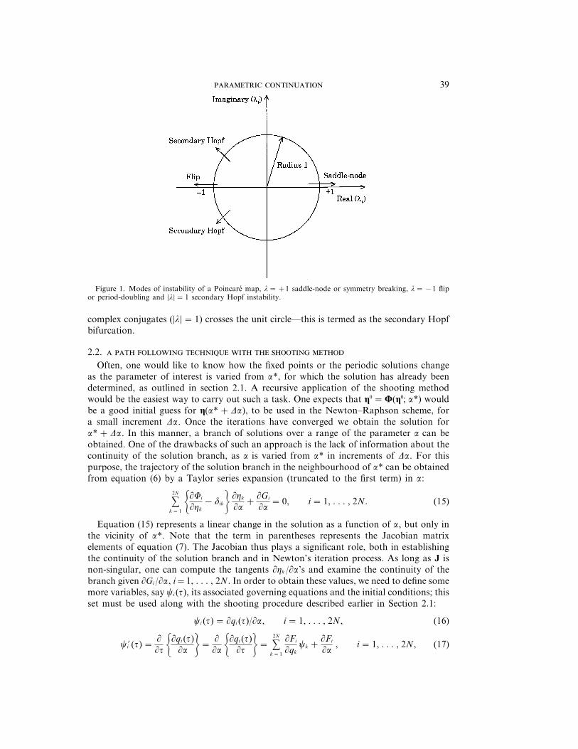
The periodic solution is stable if the magnitude of the eigenvalues, =li = (i=1, . . . , 2N),is less than unity. The stability of the periodic solution changes when some li crosses theunit circle. There are three different types of instabilities, as seen in Figure 1 (see, e.g.,references [19, 21, 25] for more details): (i) li =−1, period-doubling or flip bifurcationoccurs; (ii) li =1, saddle-node or symmetry breaking bifurcation occurs; (iii) a pair of

39

Figure 1. Modes of instability of a Poincare map, l=+1 saddle-node or symmetry breaking, l=−1 flipor period-doubling and =l==1 secondary Hopf instability.

complex conjugates (=l==1) crosses the unit circle—this is termed as the secondary Hopfbifurcation.

2.2.

Often, one would like to know how the fixed points or the periodic solutions changeas the parameter of interest is varied from a*, for which the solution has already beendetermined, as outlined in section 2.1. A recursive application of the shooting methodwould be the easiest way to carry out such a task. One expects that h0 =F(h0; a*) wouldbe a good initial guess for h(a*+Da), to be used in the Newton–Raphson scheme, fora small increment Da. Once the iterations have converged we obtain the solution fora*+Da. In this manner, a branch of solutions over a range of the parameter a can beobtained. One of the drawbacks of such an approach is the lack of information about thecontinuity of the solution branch, as a is varied from a* in increments of Da. For thispurpose, the trajectory of the solution branch in the neighbourhood of a* can be obtainedfrom equation (6) by a Taylor series expansion (truncated to the first term) in a:

s2N

k=1 61Fi

1hk− dik7 1hk

1a+

1Gi

1a=0, i=1, . . . , 2N. (15)

Equation (15) represents a linear change in the solution as a function of a, but only inthe vicinity of a*. Note that the term in parentheses represents the Jacobian matrixelements of equation (7). The Jacobian thus plays a significant role, both in establishingthe continuity of the solution branch and in Newton’s iteration process. As long as J isnon-singular, one can compute the tangents 1hk /1a’s and examine the continuity of thebranch given 1Gi /1a, i=1, . . . , 2N. In order to obtain these values, we need to define somemore variables, say ci (t), its associated governing equations and the initial conditions; thisset must be used along with the shooting procedure described earlier in Section 2.1:

ci (t)= 1qi (t)/1a, i=1, . . . , 2N, (16)

c'i (t)=1

1t 61qi (t)1a 7=

1

1a 61qi (t)1t 7= s

2N

k=1

1Fi

1qkck +

1Fi

1a, i=1, . . . , 2N, (17)

. . 40

ci (0)=0, [ i i $ [1, 2, . . . , 2N]. (18)

Comparing equations (15) and (16), we note that 1Gi /1a=ci (t0), i=1, . . . , 2N. From thecalculated tangents at a= a*, one can estimate h for a small change in the parameter, i.e.,a1 = a*+Da, as shown below:

h1*i = h0

i +1hi

1a ba*

Da, h1*i = hi (a1), i=1, . . . , 2N. (19)

This estimate is used to start the Newton iteration procedure as follows:

JDh(k+1) =−G(hk; a1), k=1, 2, . . . . (20)

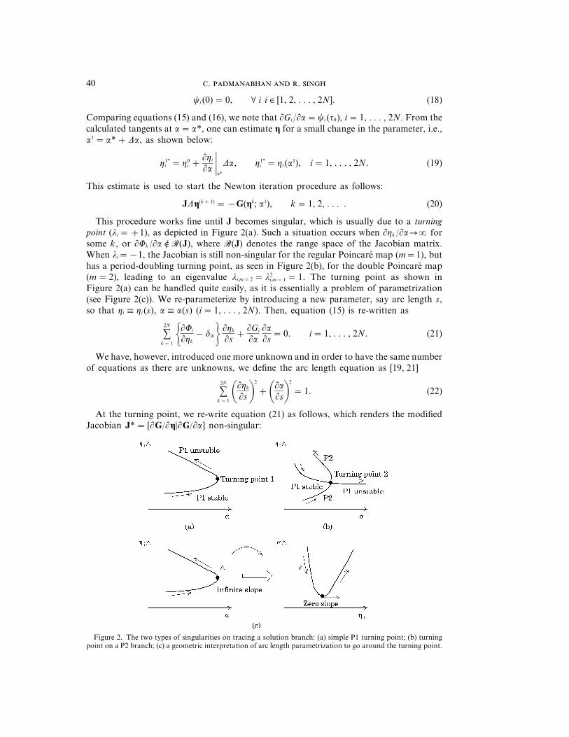
This procedure works fine until J becomes singular, which is usually due to a turningpoint (li =+1), as depicted in Figure 2(a). Such a situation occurs when 1hk /1a:a forsome k, or 1Fk /1a ( R(J), where R(J) denotes the range space of the Jacobian matrix.When li=−1, the Jacobian is still non-singular for the regular Poincare map (m=1), buthas a period-doubling turning point, as seen in Figure 2(b), for the double Poincare map(m=2), leading to an eigenvalue li,m=2 = l2

i,m=1 =1. The turning point as shown inFigure 2(a) can be handled quite easily, as it is essentially a problem of parametrization(see Figure 2(c)). We re-parameterize by introducing a new parameter, say arc length s,so that hi 0 hi (s), a0 a(s) (i=1, . . . , 2N). Then, equation (15) is re-written as

s2N

k=1 61Fi

1hk− dik7 1hk

1s+

1Gi

1a

1a

1s=0. i=1, . . . , 2N. (21)

We have, however, introduced one more unknown and in order to have the same numberof equations as there are unknowns, we define the arc length equation as [19, 21]

s2N

k=1 01hk

1s 12

+01a

1s12

=1. (22)

At the turning point, we re-write equation (21) as follows, which renders the modifiedJacobian J*= [1G/1h=1G/1a] non-singular:

Figure 2. The two types of singularities on tracing a solution branch: (a) simple P1 turning point; (b) turningpoint on a P2 branch; (c) a geometric interpretation of arc length parametrization to go around the turning point.

41

s2N

k=1

k$m

61Fj

1hk− djk7 1hk

1s+

1Gj

1a

da

ds=−61Fj

1hm− djm7 1hm

1s, j=1, . . . , 2N. (23)

At the turning point, there is a change in the direction of the parameter a. If Da waspositive (negative) to begin with, then past the turning point Da becomes negative(positive). In this manner, starting from an initial fixed point calculated as outlined insection 2.1, the procedure described above (termed continuation) can be carried out for anyparameter range, with its unique ability of going around the turning points and tracingout the entire branch of fixed point solutions; see references [19, 21, 26]. Period-doublingbranches, say P2 (period 2t0), which bifurcates from the P1 (period t0) branch, can betraced in a similar fashion once the initial P2 fixed point has been obtained using theregular shooting procedure of section 2.1, with m=2. A repeated use of this procedurewill yield P4 and other higher period solutions. The stability of the solutions is thenexamined using the monodromy matrix, B (see section 2.1.2). A uniform step size can beused over the whole parametric range, but this makes the process computationallyinefficient. Several step size control algorithms exist [26, 27]; an algorithm based on anerror estimation criterion, developed by Den Heijer and Rheinboldt [27], is used in ourstudy.

3. APPLICATION TO DUFFING OSCILLATOR

The technique developed in section 2 is illustrated and validated by applying it to acommonly used single-degree-of-freedom (SDOF) Duffing oscillator, the governingequation of which is written in the format of equation (2) as

6q'1q'27=$ 0

−k1

−j%6q1

q27+6 0−bq3

17+6 0f cos (Vt)7, (24)

where k is the linear stiffness, j is the viscous damping coefficient, b is the non-linearstiffness coefficient, f is the external sinusoidal excitation amplitude and V is the excitationfrequency. The variational equations defining mij (t), i, j=1, . . . , 2N, can be obtainedfrom equations (10) and (24) as

$m'11

m'21

m'12

m'22%=$ 0−k−3bq2

1

1−j%$m11

m21

m12

m22%. (25)

Similarly, the governing equations for ci (t) can be obtained from equations (17) and (24),when the parameter a is either the frequency V or the external excitation amplitude frespectively, as

6c'1c'27=$ 0

−k−3bq21

1−j%6c1

c27+6 0−ft sin (Vt)7, (26a)

6c'1c'27=$ 0

−k−3bq21

1−j%6c1

c27+6 0cos (Vt)7. (26b)

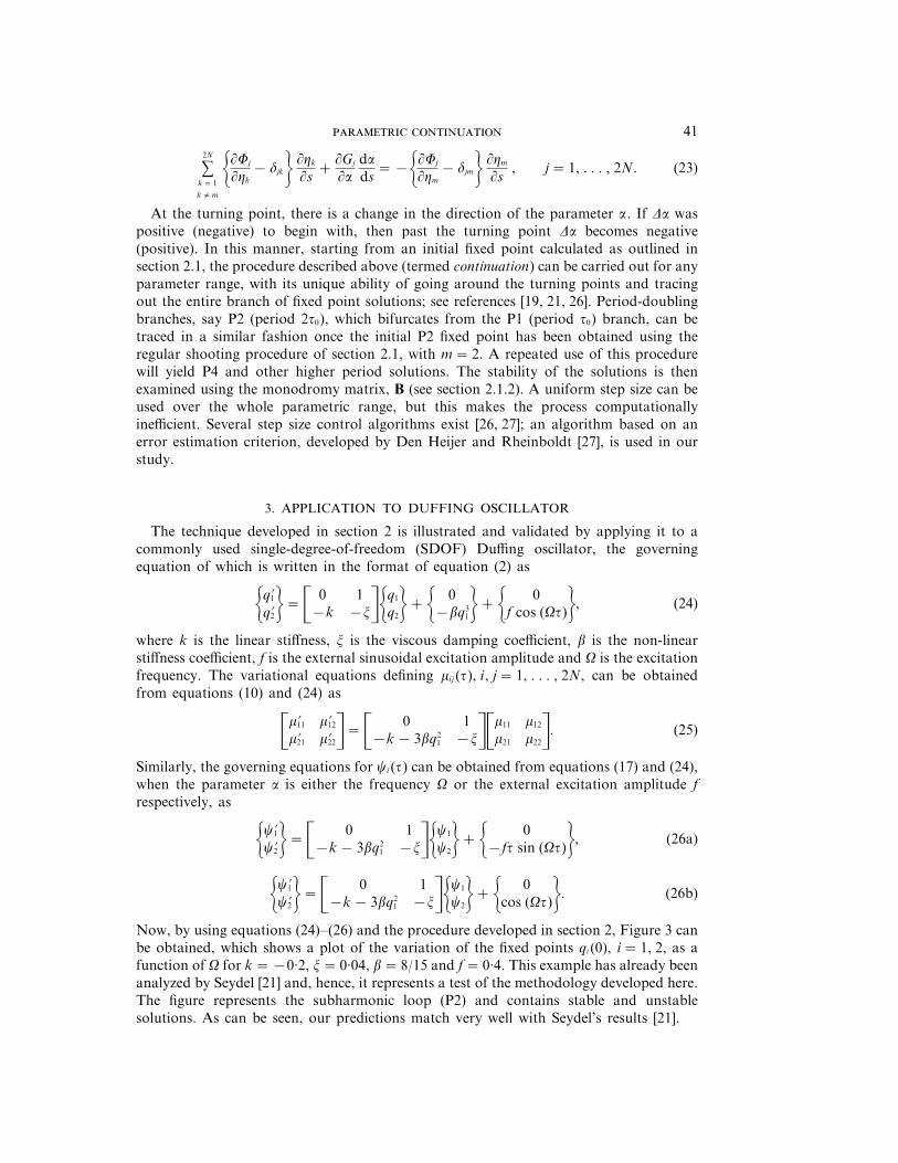
Now, by using equations (24)–(26) and the procedure developed in section 2, Figure 3 canbe obtained, which shows a plot of the variation of the fixed points qi (0), i=1, 2, as afunction of V for k=−0·2, j=0·04, b=8/15 and f=0·4. This example has already beenanalyzed by Seydel [21] and, hence, it represents a test of the methodology developed here.The figure represents the subharmonic loop (P2) and contains stable and unstablesolutions. As can be seen, our predictions match very well with Seydel’s results [21].

. . 42

Figure 3. The subharmonic loop for the Duffing oscillator: ——, proposed scheme; ×, Seydel’s scheme [21].

Next, the above equation is solved by using the continuation procedure (continuationparameter V) for three different sets of parameter values, as shown in Table 1. An initialfixed point is calculated, using the procedure in section 2.1, at a high frequency value, sayV=2 or 2·5, where the non-linear effects are negligible, and then the continuationprocedure, described in section 2.2, is started with an initial downward frequency sweep,i.e., DVQ 0. The results are shown in Figures 4–6. These are compared with thepredictions yielded by a one-term harmonic balance, which is obtained from the followingcubic equation in terms of a2, where a is the amplitude:

916b

2a6 + 32b(k−V2)a4 + {(k−V2)2 + j2V2}a2 − f 2 =0. (27)

A first order perturbation scheme [28] leads to a similar equation, but is valid only forsmall b/k values. From Figure 4(a) one can see that our procedure yields excellent

T 1

Parameter values used for the Duffing oscillator study, given j=0·04 and f=0·30

Figure b k b/k

4(a) 0·10 1·0 0·104(b) 0·75 1·0 0·75

5 and 6 0·75 0·20 3·75

43

Figure 4. The frequency response of a hardening type Duffing oscillator: (a) weakly non-linear; (b) moderatelynon-linear system. ——, Stable; – · – · – ·, unstable (+1); ×, harmonic balance (one-term) solutions.

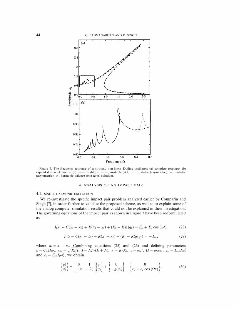
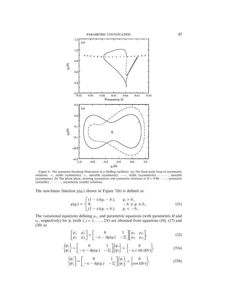
agreement with the harmonic balance or perturbation scheme. Note that there are twoturning points, one near V=1·2 and one near V=1·6. When the continuation schemegoes around these points, the fixed points change from being stable (unstable) to unstable(stable) and DV reverses signs. The three solutions regime (jump regions) predicted by bothschemes are also in good agreement. Observe in Figure 4(b) that although the matchbetween the semi-analytical and shooting method at most frequencies is still reasonable,the harmonic balance scheme cannot predict the superharmonic resonance at V1 0·33.This can obviously be remedied by introducing additional higher harmonics (such as order3, 5, etc.) in the assumed solution, but the resulting equations are more complex thanequation (27) and can only be solved by a Newton–Raphson type iteration scheme. Whenthe linear stiffness is reduced, as in Figure 5, we note that the system becomes highlynon-linear, especially at frequencies below V=0·50, and the deviation between theone-term harmonic balance and the shooting method becomes significant. A number ofsuper-harmonic resonances (of odd order 3, 5, 7, etc.) can be readily observed in Figure5(b). Also, a symmetry breaking bifurcation phenomenon (l=+1) is observed [29]. Theasymmetric solution (P1) loop around the unstable symmetric P1 solutions is shown inFigure 6(a). This phenomenon is clarified by Figure 6(b), where the phase plane portraitis shown for the symmetric (unstable) as well as the asymmetric (stable) solutions forV=0·40.

. . 44

Figure 5. The frequency response of a strongly non-linear Duffing oscillator: (a) complete response; (b)expanded view of inset in (a). ——, Stable; – · – · – ·, unstable (+1); · · · · ·, stable (asymmetric); +, unstable(asymmetric); ×, harmonic balance (one-term) solutions.

4. ANALYSIS OF AN IMPACT PAIR

4.1.

We re-investigate the specific impact pair problem analyzed earlier by Comparin andSingh [7], in order further to validate the proposed scheme, as well as to explain some ofthe analog computer simulation results that could not be explained in their investigation.The governing equations of the impact pair as shown in Figure 7 have been re-formulatedas

I1x1 +C(x1 − x2)+K(x1 − x2)+ (K1 −K)g(q1)=Em +Ep cos (vt), (28)

I2x2 −C(x1 − x2)−K(x1 − x2)− (K1 −K)g(q1)=−Em , (29)

where q1 = x1 − x2. Combining equations (25) and (26) and defining parametersz=C/2Ivn , vn =zK1/I, I= I1I2/(I1 + I2), k=K/K1, t=vnt, V=v/vn , em =Em /Iv2

n

and ep =Ep /I1v2n , we obtain

6q'1q'27=$ 0

−k

1−2z%6q1

q27+6 0−g(q1)7+6 0

em + ep cos (Vt)7. (30)

45

Figure 6. The symmetry-breaking bifurcation in a Duffing oscillator. (a) The fixed point loop of asymmetricsolutions: ×, stable (symmetric); +, unstable (symmetric); ——, stable (asymmetric); – · –· – ·, unstable(asymmetric). (b) The phase plane, showing asymmetric and symmetric solutions at V=0·40: ——, symmetric(unstable); – · – · – ·, asymmetric (stable) solutions.

The non-linear function g(q1) shown in Figure 7(b) is defined as

g(q1)=gF

f

(1− k)(q1 − br ),0,(1− k)(q1 + br ),

q1 q br ,−br E q1 E br ,q1 Q−br .

(31)

The variational equations defining mij , and parametric equations (with parameters V andep , respectively) for ci (with i, j=1, . . . , 2N) are obtained from equations (10), (17) and(30) as

$m'11

m'21

m'12

m'22%=$ 0−k−dg(q1)

1−2z%$m11

m21

m12

m22%, (32)

6c'1c'27=$ 0

−k−dg(q1)1

−2z%6c1

c27+6 0−ept sin (Vt)7, (33a)

6c'1c'2%=$ 0

−k−dg(q1)1

−2z%6c1

c27+6 0cos (Vt)7, (33b)

. . 46

Figure 7. The model of an impact pair [7]: (a) the two-degree-of-freedom semi-definite system; (b) the clearancenon-linearity (q1 = x1 − x2).

dg(q1)=dg(q1)dq1

=gF

f

(1− k),0,(1− k),

q1 q br ,−br E q1 E br ,q1 Q−br .

(34)

The system of given equations (30)–(34) is solved by using the proposed continuationprocedure and the results are shown in Figures 8–14. The values of the parameters usedin the study are listed in Table 2. For the sake of illustration, the continuation parametera used for all these studies was the non-dimensional excitation frequency V. Here again,the initial fixed point is obtained at a high frequency value, say Vq 2·0, as the non-lineareffects are small and the initial DV is negative (downward sweep). For this system, thesecondary Hopf bifurcation phenomenon is not observed, which can be established byLiouville’s theorem [18].

In Figure 8(a), the frequency response is plotted for a heavily loaded impact pair. Sincek=0, this represents a backlash problem. The analog computer results from reference [7]are shown in the figure for comparison, and an excellent agreement between the proposed

T 2

Parameters used in this study of the impact pair, given br =1

Figures z k em ep ep /em

8 and 11(a) 0·015 0·0 0·50 0·25 0·509 and 12 0·015 0·25 0·25 0·25 1·0

10 and 11(b) 0·015 0·50 0·25 0·25 1·013, 14 and 15 0·03 0·0 0·25 0·50 2·0

47

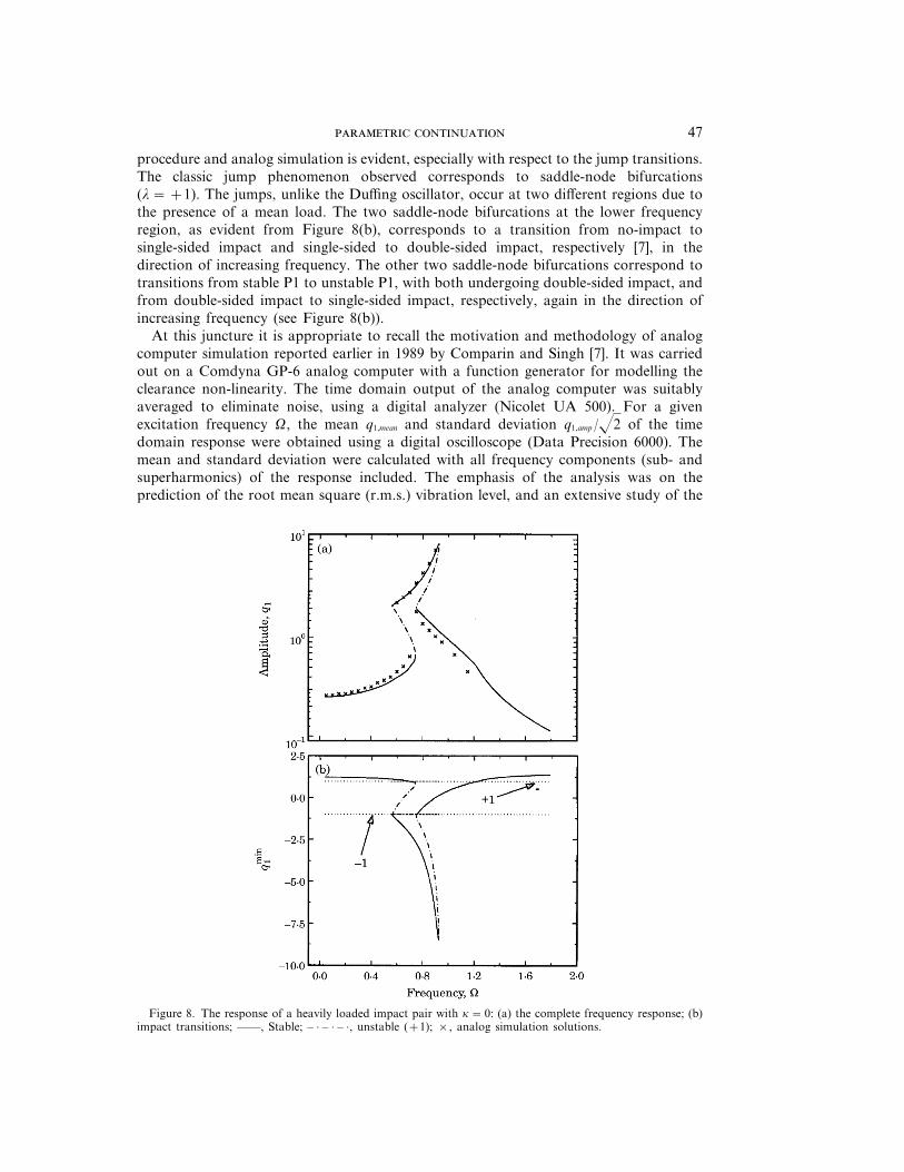
procedure and analog simulation is evident, especially with respect to the jump transitions.The classic jump phenomenon observed corresponds to saddle-node bifurcations(l=+1). The jumps, unlike the Duffing oscillator, occur at two different regions due tothe presence of a mean load. The two saddle-node bifurcations at the lower frequencyregion, as evident from Figure 8(b), corresponds to a transition from no-impact tosingle-sided impact and single-sided to double-sided impact, respectively [7], in thedirection of increasing frequency. The other two saddle-node bifurcations correspond totransitions from stable P1 to unstable P1, with both undergoing double-sided impact, andfrom double-sided impact to single-sided impact, respectively, again in the direction ofincreasing frequency (see Figure 8(b)).

At this juncture it is appropriate to recall the motivation and methodology of analogcomputer simulation reported earlier in 1989 by Comparin and Singh [7]. It was carriedout on a Comdyna GP-6 analog computer with a function generator for modelling theclearance non-linearity. The time domain output of the analog computer was suitablyaveraged to eliminate noise, using a digital analyzer (Nicolet UA 500). For a givenexcitation frequency V, the mean q1,mean and standard deviation q1,amp /z2 of the timedomain response were obtained using a digital oscilloscope (Data Precision 6000). Themean and standard deviation were calculated with all frequency components (sub- andsuperharmonics) of the response included. The emphasis of the analysis was on theprediction of the root mean square (r.m.s.) vibration level, and an extensive study of the

Figure 8. The response of a heavily loaded impact pair with k=0: (a) the complete frequency response; (b)impact transitions; ——, Stable; – · – · – ·, unstable (+1); ×, analog simulation solutions.

. . 48

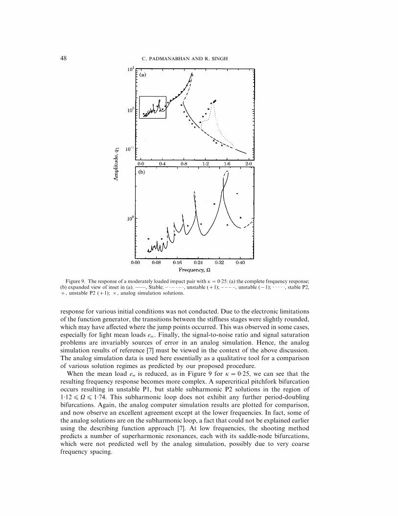
Figure 9. The response of a moderately loaded impact pair with k=0·25: (a) the complete frequency response;(b) expanded view of inset in (a). ——, Stable; – · – · – ·, unstable (+1); – – – –, unstable (−1); · · · · ·, stable P2,+, unstable P2 (+1); ×, analog simulation solutions.

response for various initial conditions was not conducted. Due to the electronic limitationsof the function generator, the transitions between the stiffness stages were slightly rounded,which may have affected where the jump points occurred. This was observed in some cases,especially for light mean loads em . Finally, the signal-to-noise ratio and signal saturationproblems are invariably sources of error in an analog simulation. Hence, the analogsimulation results of reference [7] must be viewed in the context of the above discussion.The analog simulation data is used here essentially as a qualitative tool for a comparisonof various solution regimes as predicted by our proposed procedure.

When the mean load em is reduced, as in Figure 9 for k=0·25, we can see that theresulting frequency response becomes more complex. A supercritical pitchfork bifurcationoccurs resulting in unstable P1, but stable subharmonic P2 solutions in the region of1·12EVE 1·74. This subharmonic loop does not exhibit any further period-doublingbifurcations. Again, the analog computer simulation results are plotted for comparison,and now observe an excellent agreement except at the lower frequencies. In fact, some ofthe analog solutions are on the subharmonic loop, a fact that could not be explained earlierusing the describing function approach [7]. At low frequencies, the shooting methodpredicts a number of superharmonic resonances, each with its saddle-node bifurcations,which were not predicted well by the analog simulation, possibly due to very coarsefrequency spacing.

49

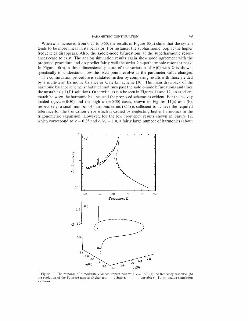
When k is increased from 0·25 to 0·50, the results in Figure 10(a) show that the systemtends to be more linear in its behavior. For instance, the subharmonic loop at the higherfrequencies disappears. Also, the saddle-node bifurcations at the superharmonic reson-ances cease to exist. The analog simulation results again show good agreement with theproposed procedure and do predict fairly well the order 2 superharmonic resonant peak.In Figure 10(b), a three-dimensional picture of the variation of qi (0) with V is shown,specifically to understand how the fixed points evolve as the parameter value changes.

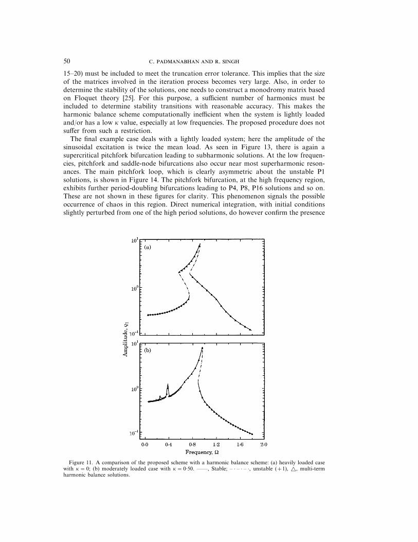
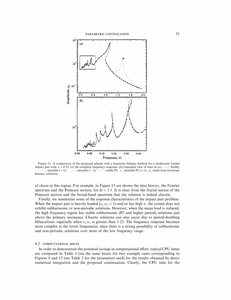
The continuation procedure is validated further by comparing results with those yieldedby a multi-term harmonic balance or Galerkin scheme [30]. The main drawback of theharmonic balance scheme is that it cannot turn past the saddle-node bifurcations and tracethe unstable (+1) P1 solutions. Otherwise, as can be seen in Figures 11 and 12, an excellentmatch between the harmonic balance and the proposed schemes is evident. For the heavilyloaded (ep /em =0·50) and the high k (=0·50) cases, shown in Figures 11(a) and (b),respectively, a small number of harmonic terms (E5) is sufficient to achieve the requiredtolerance for the truncation error which is caused by neglecting higher harmonics in thetrigonometric expansion. However, for the low frequency results shown in Figure 12,which correspond to k=0·25 and ep /em =1·0, a fairly large number of harmonics (about

Figure 10. The response of a moderately loaded impact pair with k=0·50: (a) the frequency response; (b)the evolution of the Poincare map as V changes. ——, Stable; – · – · – ·, unstable (+1); ×, analog simulationsolutions.

. . 50

15–20) must be included to meet the truncation error tolerance. This implies that the sizeof the matrices involved in the iteration process becomes very large. Also, in order todetermine the stability of the solutions, one needs to construct a monodromy matrix basedon Floquet theory [25]. For this purpose, a sufficient number of harmonics must beincluded to determine stability transitions with reasonable accuracy. This makes theharmonic balance scheme computationally inefficient when the system is lightly loadedand/or has a low k value, especially at low frequencies. The proposed procedure does notsuffer from such a restriction.

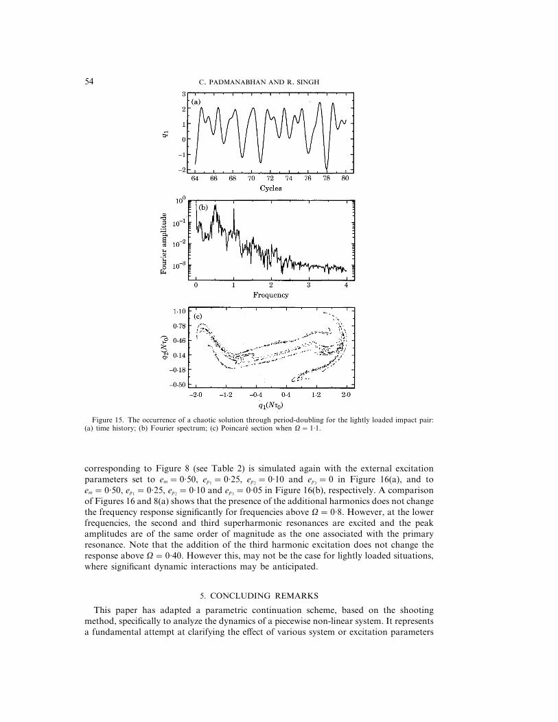
The final example case deals with a lightly loaded system; here the amplitude of thesinusoidal excitation is twice the mean load. As seen in Figure 13, there is again asupercritical pitchfork bifurcation leading to subharmonic solutions. At the low frequen-cies, pitchfork and saddle-node bifurcations also occur near most superharmonic reson-ances. The main pitchfork loop, which is clearly asymmetric about the unstable P1solutions, is shown in Figure 14. The pitchfork bifurcation, at the high frequency region,exhibits further period-doubling bifurcations leading to P4, P8, P16 solutions and so on.These are not shown in these figures for clarity. This phenomenon signals the possibleoccurrence of chaos in this region. Direct numerical integration, with initial conditionsslightly perturbed from one of the high period solutions, do however confirm the presence

Figure 11. A comparison of the proposed scheme with a harmonic balance scheme: (a) heavily loaded casewith k=0; (b) moderately loaded case with k=0·50. ——, Stable; – · – · – ·, unstable (+1), r, multi-termharmonic balance solutions.

51

Figure 12. A comparison of the proposed scheme with a harmonic balance method for a moderately loadedimpact pair with k=0·25: (a) the complete frequency response; (b) expanded view of inset in (a). ——, Stable;– · – · – ·, unstable (+1); – – – –, unstable (−1); · · · · ·, stable P2; +, unstable P2 (+1); r, multi-term harmonicbalance solutions.

of chaos in this region. For example, in Figure 15 are shown the time history, the Fourierspectrum and the Poincare section, for V=1·1. It is clear from the fractal nature of thePoincare section and the broad-band spectrum that the solution is indeed chaotic.

Finally, we summarize some of the response characteristics of the impact pair problem.When the impact pair is heavily loaded (ep /em Q 1) and/or has high k, the system does notexhibit subharmonic or non-periodic solutions. However, when the mean load is reduced,the high frequency region has stable subharmonic (P2 and higher period) solutions justabove the primary resonance. Chaotic solutions can also occur due to period-doublingbifurcations, especially when ep /em is greater than 1·25. The frequency response becomesmost complex at the lower frequencies, since there is a strong possibility of subharmonicand non-periodic solutions over most of the low frequency range.

4.2.

In order to demonstrate the potential savings in computational effort, typical CPU timesare compared in Table 3 (on the same basis) for two example cases corresponding toFigures 8 and 13 (see Table 2 for the parameters used) for the results obtained by directnumerical integration and the proposed continuation. Clearly, the CPU time for the

. . 52

T 3

A comparison of classical numerical integration with the continuation method

Issue Classical integration Continuation

Multi-valued and Large initial condition map Initial point alone needsunstable solutions needs to be searched; some effort; other points

unstable solutions can be obtained quite efficiently,obtained only by integration including subharmonic andin negative time unstable solutions

Example case CPU times for 250 parameter points:(a) Figure 8 3000 s 185 s(b) Figure 13 7400 s 295 s

continuation procedure is at least an order of magnitude smaller than that required forclassical numerical integration. This is primarily because the direct numerical integrationprocedure needs to be carried out for several time periods of the excitation, in order toachieve steady state conditions. Note that in order to obtain the unstable results by directnumerical integration one has to integrate in negative time as well. Also, in order to find

Figure 13. The frequency response for a lightly loaded impact pair for k=0: (a) the complete response; (b)expanded view of the inset in (a). ——, Stable; – · – · – ·, unstable (+1); – – – –, unstable (−1); · · · · ·, unstableP2 (+1); +, stable P2; r, unstable P2 (−1) solutions.

53

Figure 14. The subharmonic fixed point solution loop for a lightly loaded impact pair with k=0: (a) q1(0)versus V; (b) q2(0) versus V. ——, Stable P2; – · – · – ·, unstable P2 (+1); · · · · ·, unstable P2 (−1); r, stableP1; q, unstable P1 (+1); ×, unstable P1 (−1) solutions.

subharmonic, quasi-periodic or chaotic solutions, a large initial condition map must besearched, since we do not have an a priori knowledge of which parameter regions exhibitsuch phenomena. Conversely, in the proposed procedure, such regimes are found moreefficiently. For example, the occurrence of a period-doubling bifurcation during thecontinuation process (l=−1) signals the possible occurrence of stable P2, higher periodsubharmonic solutions or even chaotic solutions through the Feigenbaum cascade [19, 21].Using values of m=2, 4, etc., in the method described in section 2, one can then obtainthe subharmonic solutions and the period-doubling cascade. Similar procedures may alsobe established for other types of solutions.

4.3. -

In the previous sections, all of the example cases were for a single harmonic excitationonly. However, the formulation developed in section 2 is valid for any periodic excitationthat can be represented by a Fourier series in terms of the fundamental excitationfrequency V. To illustrate this point, we consider one example of a multi-harmonicexcitation of the impact pair. In equation (29), the term ep cos (Vt) is replaced bysM

k=1 epk cos (kVt), where M is the number of harmonics in the excitation. The system

. . 54

Figure 15. The occurrence of a chaotic solution through period-doubling for the lightly loaded impact pair:(a) time history; (b) Fourier spectrum; (c) Poincare section when V=1·1.

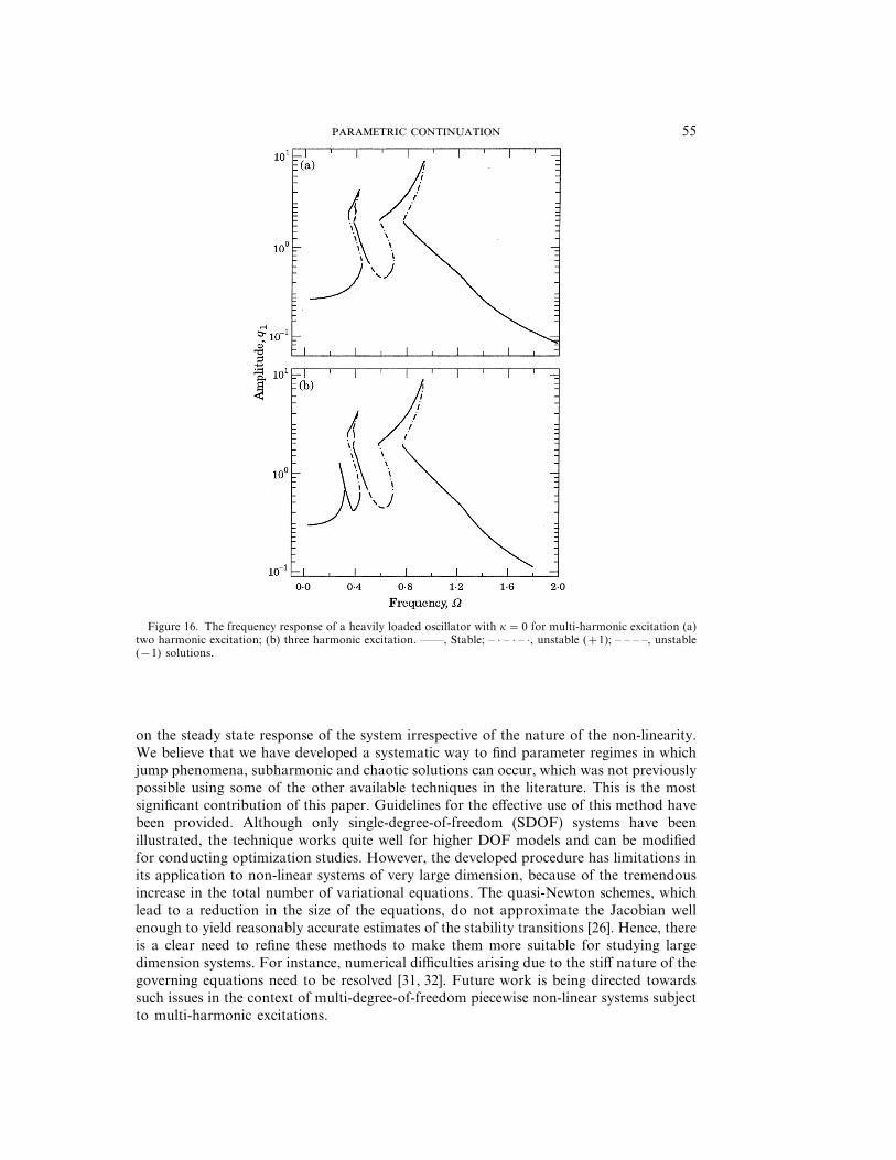
corresponding to Figure 8 (see Table 2) is simulated again with the external excitationparameters set to em =0·50, ep1 =0·25, ep2 =0·10 and ep3 =0 in Figure 16(a), and toem =0·50, ep1 =0·25, ep2 =0·10 and ep3 =0·05 in Figure 16(b), respectively. A comparisonof Figures 16 and 8(a) shows that the presence of the additional harmonics does not changethe frequency response significantly for frequencies above V=0·8. However, at the lowerfrequencies, the second and third superharmonic resonances are excited and the peakamplitudes are of the same order of magnitude as the one associated with the primaryresonance. Note that the addition of the third harmonic excitation does not change theresponse above V=0·40. However this, may not be the case for lightly loaded situations,where significant dynamic interactions may be anticipated.

5. CONCLUDING REMARKS

This paper has adapted a parametric continuation scheme, based on the shootingmethod, specifically to analyze the dynamics of a piecewise non-linear system. It representsa fundamental attempt at clarifying the effect of various system or excitation parameters

55

Figure 16. The frequency response of a heavily loaded oscillator with k=0 for multi-harmonic excitation (a)two harmonic excitation; (b) three harmonic excitation. ——, Stable; – · – · – ·, unstable (+1); – – – –, unstable(−1) solutions.

on the steady state response of the system irrespective of the nature of the non-linearity.We believe that we have developed a systematic way to find parameter regimes in whichjump phenomena, subharmonic and chaotic solutions can occur, which was not previouslypossible using some of the other available techniques in the literature. This is the mostsignificant contribution of this paper. Guidelines for the effective use of this method havebeen provided. Although only single-degree-of-freedom (SDOF) systems have beenillustrated, the technique works quite well for higher DOF models and can be modifiedfor conducting optimization studies. However, the developed procedure has limitations inits application to non-linear systems of very large dimension, because of the tremendousincrease in the total number of variational equations. The quasi-Newton schemes, whichlead to a reduction in the size of the equations, do not approximate the Jacobian wellenough to yield reasonably accurate estimates of the stability transitions [26]. Hence, thereis a clear need to refine these methods to make them more suitable for studying largedimension systems. For instance, numerical difficulties arising due to the stiff nature of thegoverning equations need to be resolved [31, 32]. Future work is being directed towardssuch issues in the context of multi-degree-of-freedom piecewise non-linear systems subjectto multi-harmonic excitations.

. . 56

ACKNOWLEDGMENTS

The authors wish to acknowledge the primary support from the U.S. Army ResearchOffice (URI Grant DAAL 03-92-G-0120; 1992–97; Project Monitor Dr T. L. Doligalski),as well as additional support from the Nissan Technical Center (Japan) and the Centerfor Automotive Research at The Ohio State University. The first author is indebted toProfessor G. R. Baker of The Ohio State University for introducing him to the techniquesused in this paper. Thanks are also due to Dr R. J. Comparin for sharing the analogcomputer results.

REFERENCES

1. K. K and F. P 1991 Nonlinear Dynamics 2, 367–387. Theoretical andexperimental investigations of gear-rattling.

2. J. S and S. W. S 1989 Transactions of the American Society of Mechanical Engineers,Journal of Applied Mechanics 56, 168–174. The onset of chaos in a two-degree-of-freedomimpacting system.

3. H. S. C and J. Y. K. L 1991 International Journal of Nonlinear Mechanics 26, 461–473.Nonlinear behavior and chaotic motions of an SDOF system with piecewise-nonlinear stiffness.

4. Y. B. K and S. T. N 1991 Transactions of the American Society of Mechanical Engineers,Journal of Applied Mechanics 58, 545–553. Stability and bifurcation analysis of oscillators withpiecewise-linear characteristics: a general approach.

5. C. W. W, W. S. Z and S L. L 1991 Journal of Sound and Vibration 149, 91–105.Periodic forced vibration of unsymmetric piecewise-linear systems by incremental harmonicbalance method.

6. M. K, S. O and T. S 1991 Japan Society of Mechanical Engineers,International Journal Series III 34, 345–354. Forced torsional vibration of a two-degree-of-free-dom system including a clearance and two-step-hardening spring.

7. R. J. C and R. S 1989 Journal of Sound and Vibration 134, 259–290. Non-linearfrequency response characteristics of an impact pair.

8. M. A. V and F. R. E. C 1975 Transactions of the American Society ofMechanical Engineers, Journal of Engineering for Industry 97, 820–827. Multiple impacts of aball between two plates, part 1: some experimental observations.

9. M. A. V, F. R. E. C and G. H 1975 Transactions of the American Societyof Mechanical Engineers, Journal of Engineering for Industry 97, 828–835. Multiple impacts ofa ball between two plates, part 1: some mathematical modeling.

10. R. S, H. X and R. J. C 1989 Journal of Sound and Vibration 131, 177–196.Analysis of automotive neutral gear rattle.

11. A. K and R. S 1991 Journal of Sound and Vibration 144, 469–506. Non-lineardynamics of a geared rotor-bearing system with multiple clearances.

12. R. J. C and R. S 1990 Journal of Sound and Vibration 142, 101–124. Frequencyresponse characteristics of a multi-degree-of-freedom system with clearances.

13. M. U and A. R 1966 Journal of Mathematical Analysis and Applications 14, 107–140.Numerical computation of nonlinear forced oscillations by Galerkin’s procedure.

14. A. G and W. E. V V 1968 Multiple-Input Describing Functions and NonlinearSystems Design. New York: McGraw-Hill.

15. F. H. L 1983 Applied Mathematics and Mechanics (English edition) 4, 525–546. A numericaltreatment of the periodic solutions of non-linear vibration systems.

16. S. F and J. M. T. T 1991 Computer Methods in Applied Mechanics and Engineering89, 381–394. Geometrical concepts and computational techniques of nonlinear dynamics.

17. J. A and T. S 1991 Journal of Sound and Vibration 146, 527–532. Periodic,quasi-periodic and chaotic orbits and their bifurcations in a system of coupled oscillators.

18. K. S, S. Y and T. K 1991 Computational Mechanics 7, 173–182.Bifurcation sets and chaotic states of a gear system subject to harmonic excitation.

19. M. K and M. M 1983 Computational Methods in Bifurcation Theory and DissipativeStructures. New York: Springer-Verlag.

20. M. H and M. K 1984 Journal of Computational Physics 55, 254–267.DERPER—an algorithm for continuation of periodic solutions in ordinary differentialequations.

57

21. R. S 1988 From Equilibrium to Chaos: Practical Bifurcation and Stability Analysis. NewYork: Elsevier.

22. J. R. D and P. J. P 1978 Celestial Mechanics 18, 223–232. New Runge–Kuttaalgorithms for numerical simulation in dynamical astronomy.

23. C. G B 1969 Computer Journal 12, 94–99. A new method of solving non-linearsimultaneous equations.

24. M. R. M 1976 Journal of Optimization Theory and Applications 20, 37–46. On Warner’salgorithm for the solution of boundary-value problems for ordinary differential equations.

25. G. I and D. D. J 1980 Elementary Stability and Bifurcation Theory. New York:Springer-Verlag.

26. E. L. A and K. G 1990 Numerical Continuation Methods: an introduction. NewYork: Springer-Verlag.

27. C. D H and W. C. R 1981 SIAM Journal of Numerical Analysis 18, 925–948.On steplength algorithms for a class of continuation methods.

28. A. H. N and D. T. M 1979 Nonlinear Oscillations. New York: John Wiley.29. J. M 1989 SIAM Journal of Applied Mathematics 49, 968–981. Resonance and symmetry

breaking for a Duffing oscillator.30. F. H. L and X. X. W 1987 International Journal of Nonlinear Mechanics 22, 89–98. Fast

Galerkin method and its application to determine periodic solutions of non-linear oscillators.31. E. H, S. P. N and G. W 1987 Solving Ordinary Differential Equations II—Stiff

Problems. Berlin: Springer-Verlag.32. C. P,R.C.B, T.E.R and R. S 1995 American Society of Mechanical

Engineers, Journal of Mechanical Design 117, 185–192. Computational Issues Associated withGear Rattle Analysis.

APPENDIX A: LIST OF SYMBOLS

a sinusoidal amplitude term for Duffing oscillatorA linear state matrixbr transition from first to second stage stiffness of the impact pairB monodromy matrixC viscous damping for the impact paire normalized excitation force on impact pairE excitation force on the impact pairf excitation amplitude for Duffing oscillatorF general force vectorg non-linear force function for the impact pairG general non-linear function vectorh general non-linear force vectorI1 first inertia of the impact pairI2 second inertia of the impact pairI combined inertia term for the impact pairJ Jacobian matrixk linear stiffness term for Duffing oscillatorK first stage stiffness of the impact pairK1 second stage stiffness of the impact pairM number of excitation harmonicsN number of degrees of freedom of any systemq state vector

s arc length parameterT external excitation vectorxi displacements of impact pair; i=1, 2a parametera* parameter value at fixed pointb cubic stiffness coefficient for Duffing oscillatord Kronecker deltaF state vector magnitude at t0

k ratio of the first and second stage stiffness for the impact pairl eigenvalue of monodromy matrix

. . 58

u homotopy parameterm derivative matrix of the state vector with respect to (w.r.t.) hh initial condition vectorh0 fixed point vectort timet0 fundamental time periodvn normalizing frequency for impact pairV fundamental excitation frequencyj viscous damping coefficient for Duffing oscillatorC derivative vector of state vector w.r.t. parameter az non-dimensional viscous damping coefficient of impact pair

Subscripts

m meanp alternating componentsamp amplitudei, j, k vector or matrix indices

Second order subscripts

i excitation harmonic index

Superscripts

1, 1* corrector step in the continuation schemek iteration step in Newton–Raphson scheme

Symbols

D correction or change in any parameter=·= magnitude