1

Analysis of images on PHENOPSIS DB using ImageJ Analysis of images on PHENOPSIS DB using ImageJ Analysis of images on PHENOPSIS DB using ImageJ Analysis of images on PHENOPSIS DB using ImageJ macrosmacrosmacrosmacros

VersionVersionVersionVersion 1.2 (031.2 (031.2 (031.2 (03----2015)2015)2015)2015)

1. Aim1. Aim1. Aim1. Aim

ImageJ macros have been composed at LEPSE (INRA, Montpellier, France) for the semi-automatic analysis of images present in the Phenopsis database. Visible images of rosettes, taken automatically by the PHENOPSIS automaton, and scans of individual leaves, dissected from rosettes, can be analysed for surface area, perimeter, width and height. A visible / infra-red macro is being developed allowing the extraction of temperature data from infra-red images taken automatically by the PHENOPSIS automaton. References

• PHENOPSIS DB : http://bioweb.supagro.inra.fr/phenopsis • ImageJ : http://rsb.info.nih.gov/ij

2. Installation2. Installation2. Installation2. Installation

One can choose to install the PHENOPSIS version of ImageJ, which includes the required plugins and macros, or to put the PHENOPSIS macros and toolset in an existing version of ImageJ. The latter option requires that certain plugins are present in the ImageJ version. In both cases, one needs to make sure that Java is updated. 2.1 Installation of ImageJ_Phenopsis on your computer2.1 Installation of ImageJ_Phenopsis on your computer2.1 Installation of ImageJ_Phenopsis on your computer2.1 Installation of ImageJ_Phenopsis on your computer

2

•••• Put the “ImageJ_Phenopsis” file in an appropriate location on your computer, for example C:\Program Files. You can keep your own version of ImageJ (with your specific plugins) already installed on your computer.

•••• Create a shortcut from “ImageJ_Phenopsis.exe” in the file “ImageJ_Phenopsis”. •••• Open “\ImageJ_Phenopsis\macros\StartupMacros.txt”. Check the file paths of the

different Action Tools and, if required, change them your specific configuration. 2.2 Installation of the Phenopsis macros in an existing version of ImageJ on your 2.2 Installation of the Phenopsis macros in an existing version of ImageJ on your 2.2 Installation of the Phenopsis macros in an existing version of ImageJ on your 2.2 Installation of the Phenopsis macros in an existing version of ImageJ on your computercomputercomputercomputer

•••• Put the “Phenopsis” folder in the “\ImageJ\macros\” folder on your computer. •••• Put the “Phenopsis.txt” file in the “\ImageJ\macros\toolsets\” folder on your

computer. •••• Put the “Threshold colour.jar” file in the “\ImageJ\plugins\” folder. •••• Put the “TurboReg_StackAlign.jar” file in the “\ImageJ\plugins\” folder •••• Open “\ImageJ\macros\toolsets\Phenopsis.txt”. Check the file paths of the different

Action Tools and, if required, change them your specific configuration.

3. Updates3. Updates3. Updates3. Updates

• Check the PHENOPSIS DB website for updates of the macros and this manual. • Use the “ImageJ updater” plugin to regularly check for new versions of ImageJ

(check the “testing” box, not the “stable” one).

3

4. Image analysis4. Image analysis4. Image analysis4. Image analysis

When you open ImageJ_Phenopsis, it looks like this : If you have kept your own version of ImageJ, you should go and look for the “Phenopsis” toolset by clicking on the arrows on the far right (“Switch to alternate macro tool sets”). At the moment, 8 macros are available:

• Rosette surface area analysis:

• Rosette surface area selection:

• Leaf surface area analysis:

• Leaf surface area selection:

• Image calibration:

• A seventh macro is in a testing phase: Visible-IR image overlay and

analysis:

• Fluorescence_NIR macro:

• Fluorescence_FV macro :

4

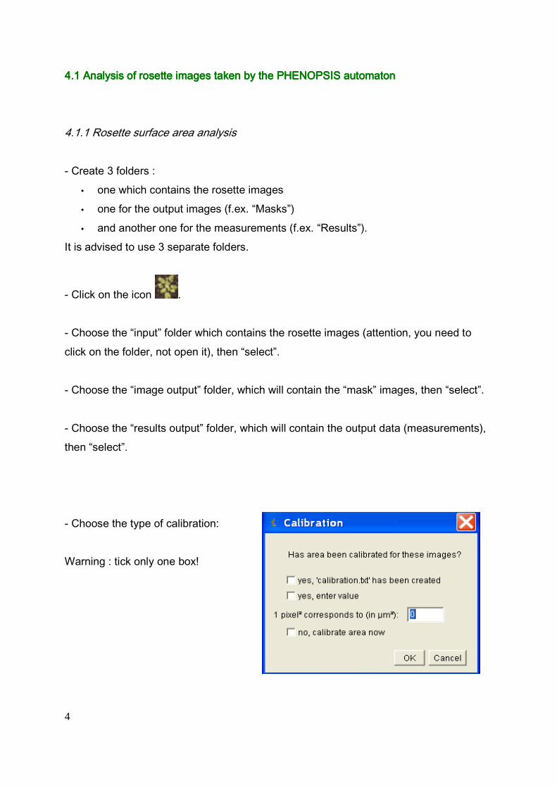
4.1 Analysis of rosette images taken by the PHENOPSIS automaton4.1 Analysis of rosette images taken by the PHENOPSIS automaton4.1 Analysis of rosette images taken by the PHENOPSIS automaton4.1 Analysis of rosette images taken by the PHENOPSIS automaton 4.1.1 Rosette surface area analysis - Create 3 folders :

• one which contains the rosette images • one for the output images (f.ex. “Masks”) • and another one for the measurements (f.ex. “Results”).

It is advised to use 3 separate folders.

- Click on the icon . - Choose the “input” folder which contains the rosette images (attention, you need to click on the folder, not open it), then “select”. - Choose the “image output” folder, which will contain the “mask” images, then “select”. - Choose the “results output” folder, which will contain the output data (measurements), then “select”. - Choose the type of calibration: Warning : tick only one box!

5

Option 1Option 1Option 1Option 1 The “calibration.txt” already exists in the image input folder, which means that you have

already used the “Image calibration” macro for this dataset. Option 2Option 2Option 2Option 2 A known calibration is entered here; there 2 options:

• either one leaves the value at 0, which means output data will be reported in a number of pixels only;

• or one fills out the value of a square pixel in mm². Option 3Option 3Option 3Option 3 There hasn’t been any calibration done yet.

The “Image calibration” macro is launched automatically. Follow the instructions in the popup windows:

• open the image which contains the calibration reference (f.ex. millimetre paper) • delimit a calibration area using the ImageJ selection tools ( ) • and enter the corresponding value in mm or mm².

A “calibration.txt” is created in the folder which contained the calibration image. Warning: this should be your image “input” folder! The macro continues automatically now. ATTENTIONATTENTIONATTENTIONATTENTION : The macro starts and continues automatically. If a problem is detected, the macro can be stopped by closing an image on screen. The output file “Summary results.xls” will have been created with the results for the images processed so far.

6

On the other hand, upon restart of the macro, the complete folder will be reanalysed. The main output file is “Summary results.xls”, which contains the surface area data per image. For each image, a separate file is created which contains the measured data for each object detected in the image (f.ex. multiple rosettes). The “Rosette surface area selection” can now be used to check the detected objects. 4.1.2 Rosette surface area selection This macro can be used to check the objects detected by the “Rosette surface area analysis” macro. This means :

• to select the rosette(s) of interest, • to separate touching rosettes (detected as one object) • or to draw and measure any rosette that wasn’t detected by the macro (f.ex. very

small rosettes, often lighter green).

- Click on the icon - Choose the “input” folder which contains the rosette images (attention, you need to click on the folder, not open it), then “select”. - Choose the “image output” folder, which contains the “mask” images, then “select”. - Choose the “results output” folder, which contains the output data (measurements), then “select”. - Choose the type of calibration (see above). - Choose a module in the “Rosette selection” window:

7

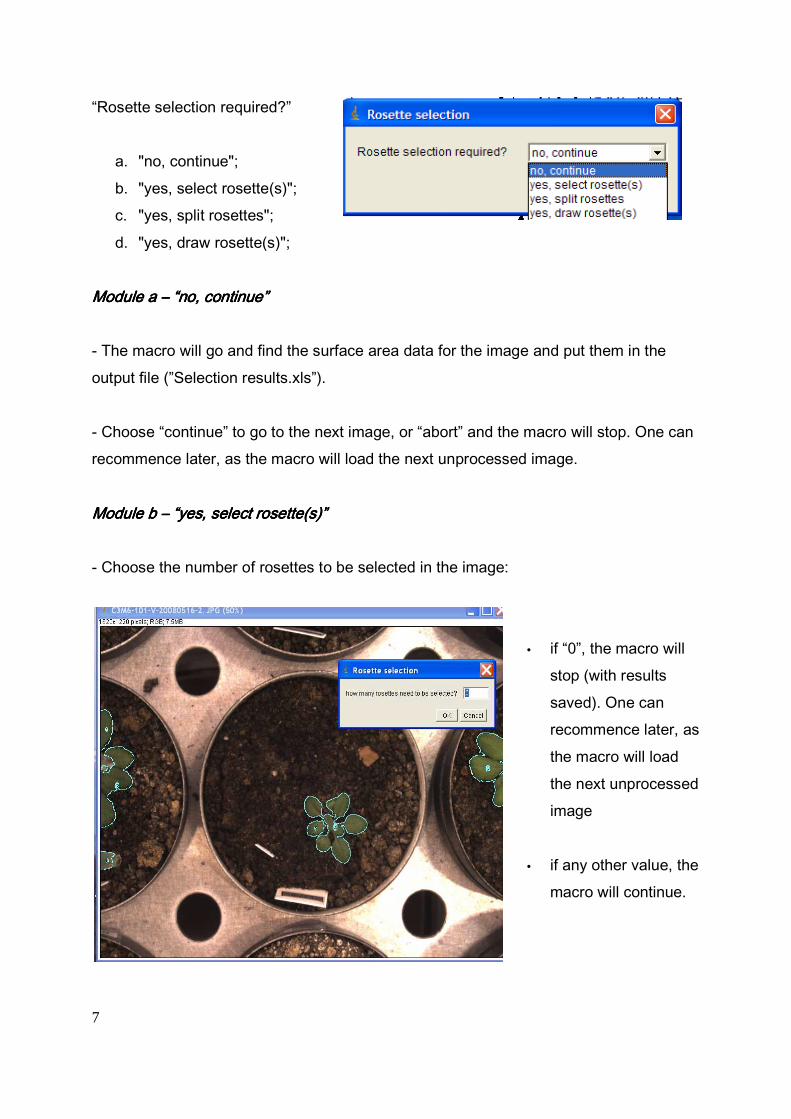
“Rosette selection required?”

a. "no, continue"; b. "yes, select rosette(s)"; c. "yes, split rosettes"; d. "yes, draw rosette(s)";

Module a Module a Module a Module a –––– “no, continue”“no, continue”“no, continue”“no, continue” - The macro will go and find the surface area data for the image and put them in the output file (”Selection results.xls”). - Choose “continue” to go to the next image, or “abort” and the macro will stop. One can recommence later, as the macro will load the next unprocessed image. Module b Module b Module b Module b –––– “yes, select rosette(s)”“yes, select rosette(s)”“yes, select rosette(s)”“yes, select rosette(s)” - Choose the number of rosettes to be selected in the image:

• if “0”, the macro will stop (with results saved). One can recommence later, as the macro will load the next unprocessed image

• if any other value, the

macro will continue.

8

- For each rosette: enter an indicator (f.ex. “left” or “middle” or “right”). Choose to fill out the box with the “Region of interest (Roi)” numbers which are shown in the image, or to do a selection, in case a rosette is very fragmented (leave the number box “0” and click “ok”). In the latter case, put a contour round the rosette of interest and click “ok”. The surface area of the rosette of interest is saved in the output file (”Selection results.xls”).

- Choose “continue” to go to the next image, or “abort” and the macro will stop. One can recommence later, as the macro will load the next unprocessed image.

9

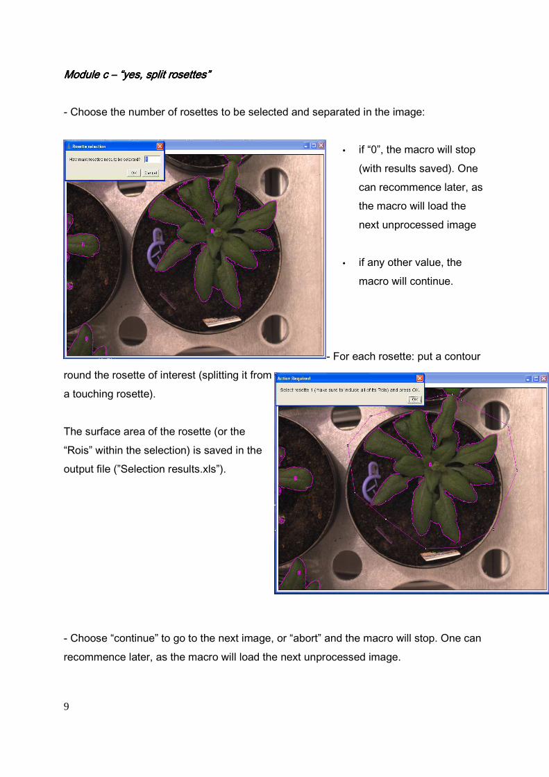
Module c Module c Module c Module c –––– “yes, split ros“yes, split ros“yes, split ros“yes, split rosettes”ettes”ettes”ettes” - Choose the number of rosettes to be selected and separated in the image:

• if “0”, the macro will stop

(with results saved). One can recommence later, as the macro will load the next unprocessed image

• if any other value, the

macro will continue. - For each rosette: put a contour

round the rosette of interest (splitting it from a touching rosette). The surface area of the rosette (or the “Rois” within the selection) is saved in the output file (”Selection results.xls”).

- Choose “continue” to go to the next image, or “abort” and the macro will stop. One can recommence later, as the macro will load the next unprocessed image.

10

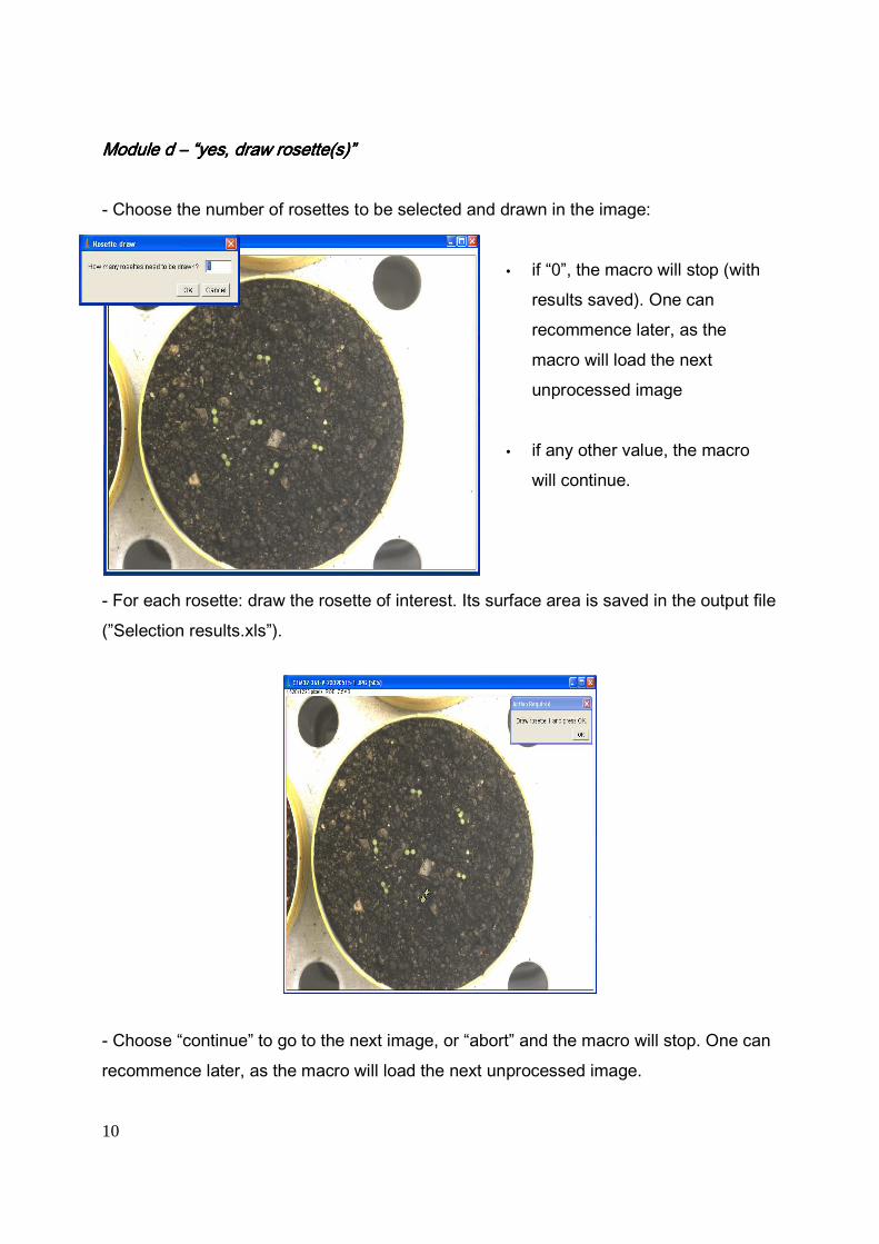
Module d Module d Module d Module d –––– “yes, draw rosette(s)”“yes, draw rosette(s)”“yes, draw rosette(s)”“yes, draw rosette(s)” - Choose the number of rosettes to be selected and drawn in the image:

• if “0”, the macro will stop (with

results saved). One can recommence later, as the macro will load the next unprocessed image

• if any other value, the macro

will continue.

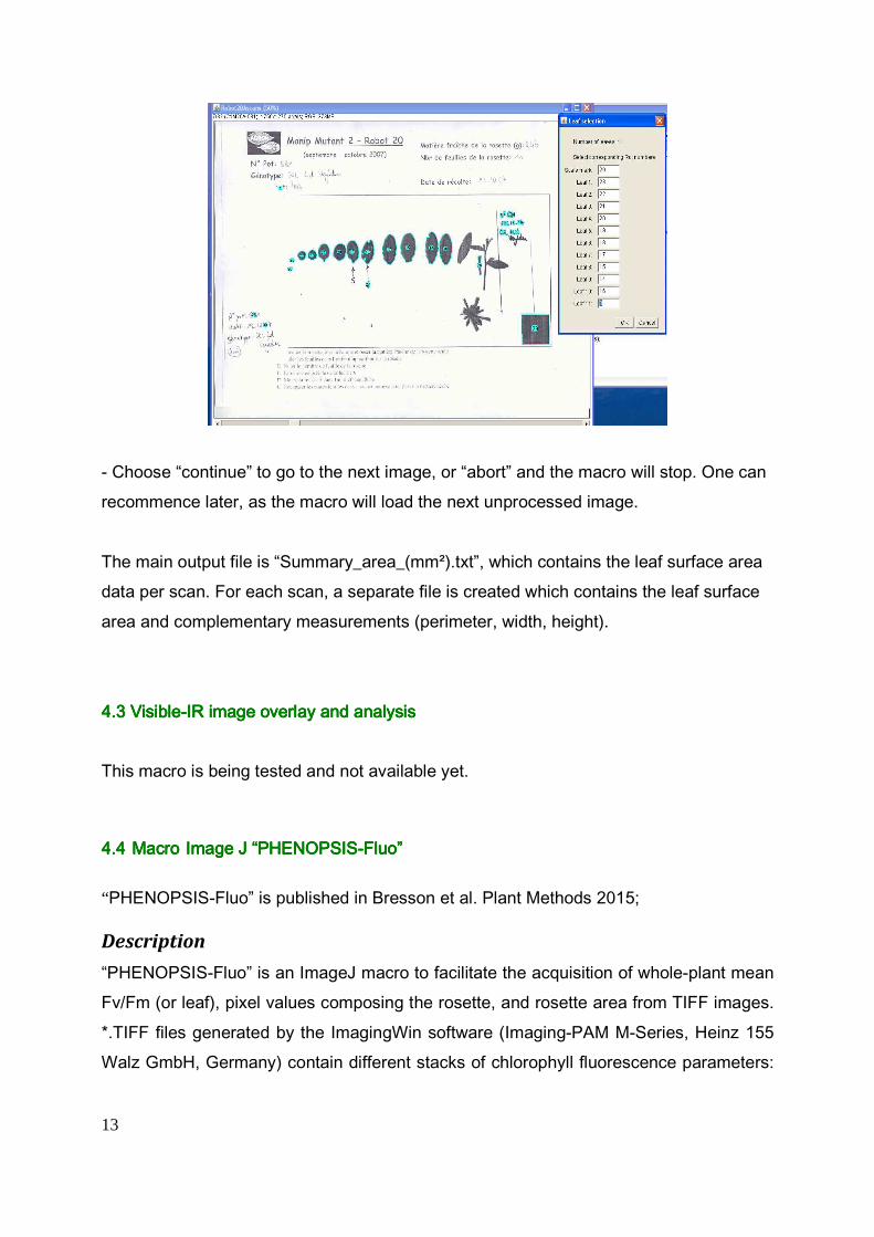
- For each rosette: draw the rosette of interest. Its surface area is saved in the output file (”Selection results.xls”).

- Choose “continue” to go to the next image, or “abort” and the macro will stop. One can recommence later, as the macro will load the next unprocessed image.

11

4.2 Analysis of scans of leaves dissected from a ro4.2 Analysis of scans of leaves dissected from a ro4.2 Analysis of scans of leaves dissected from a ro4.2 Analysis of scans of leaves dissected from a rosettesettesettesette 4.2.1 Leaf surface area analysis - Create 2 folders: one for the leaf scans and one for the measurements (f.ex. “Results”). It is advised to use two separate folders. Attention: all the scans in the folder should be oriented in the same way (f.ex. calibration mark in bottom right corner)!

- Click on the icon - Choose the “input” folder which contains the leaf scans (attention, you need to click on the folder, not open it), then “select”. - Choose the “results output” folder, which will contain the output data (measurements), then “select”. - Choose the position of the calibration mark. If there isn’t any calibration mark in the scans, choose “no calibration mark”. In this case, the scans are treated as A4 pages (297*210 mm²). The macro will continue automatically. At the end, when all scans in the folder are processed, it will propose to continue with the “leaf surface area selection” macro, to attribute leaf rank numbers to the objects detected in the scans. 4.2.2 Leaf surface area selection

- Click on the icon .

12

- Choose the “input” folder which contains the leaf scans (attention, you need to click on the folder, not open it), then “select”. - Choose the “results output” folder, which contains the output data (measurements), then “select”. - Choose the position of the calibration mark and enter the surface area of the calibration mark in mm². If there isn’t any calibration mark in the scans, choose “no calibration mark”. In this case, the scans are treated as A4 pages (297*210 mm²). - Fill out the number of leaves in the scan and click “ok”.

- Fill out in the boxes the number of the Roi, as shown in the image, corresponding to the calibration mark and the leaf rank. Then click “ok”. “Tab” can be used to go from one box to the next. One can leaf boxes “0” for leaf ranks missing in the scan.

13

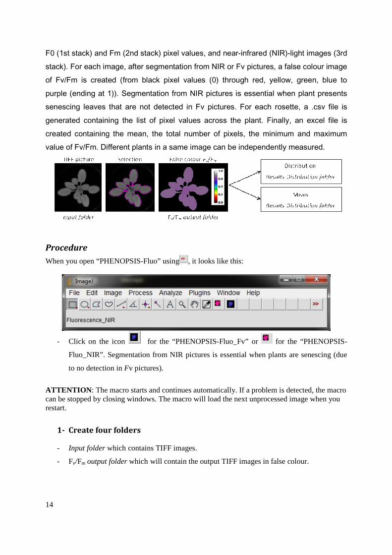
- Choose “continue” to go to the next image, or “abort” and the macro will stop. One can recommence later, as the macro will load the next unprocessed image. The main output file is “Summary_area_(mm²).txt”, which contains the leaf surface area data per scan. For each scan, a separate file is created which contains the leaf surface area and complementary measurements (perimeter, width, height). 4.3 Visible4.3 Visible4.3 Visible4.3 Visible----IR image overlay and analysisIR image overlay and analysisIR image overlay and analysisIR image overlay and analysis This macro is being tested and not available yet.

4.44.44.44.4 MacroMacroMacroMacro Image J “PHENOPSISImage J “PHENOPSISImage J “PHENOPSISImage J “PHENOPSIS----Fluo”Fluo”Fluo”Fluo”

“PHENOPSIS-Fluo” is published in Bresson et al. Plant Methods 2015;

Description

“PHENOPSIS-Fluo” is an ImageJ macro to facilitate the acquisition of whole-plant mean Fv/Fm (or leaf), pixel values composing the rosette, and rosette area from TIFF images. *.TIFF files generated by the ImagingWin software (Imaging-PAM M-Series, Heinz 155 Walz GmbH, Germany) contain different stacks of chlorophyll fluorescence parameters:

14

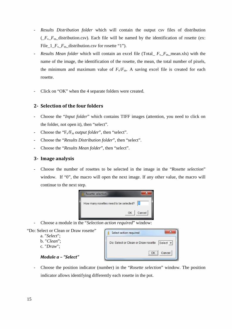
F0 (1st stack) and Fm (2nd stack) pixel values, and near-infrared (NIR)-light images (3rd stack). For each image, after segmentation from NIR or Fv pictures, a false colour image of Fv/Fm is created (from black pixel values (0) through red, yellow, green, blue to purple (ending at 1)). Segmentation from NIR pictures is essential when plant presents senescing leaves that are not detected in Fv pictures. For each rosette, a .csv file is generated containing the list of pixel values across the plant. Finally, an excel file is created containing the mean, the total number of pixels, the minimum and maximum value of Fv/Fm. Different plants in a same image can be independently measured.

Procedure

When you open “PHENOPSIS-Fluo” using, it looks like this:

- Click on the icon for the “PHENOPSIS-Fluo_Fv” or for the “PHENOPSIS-

Fluo_NIR”. Segmentation from NIR pictures is essential when plants are senescing (due

to no detection in Fv pictures).

ATTENTION: The macro starts and continues automatically. If a problem is detected, the macro can be stopped by closing windows. The macro will load the next unprocessed image when you restart.

1- Create four folders

- Input folder which contains TIFF images.

- Fv/Fm output folder which will contain the output TIFF images in false colour.

15

- Results Distribution folder which will contain the output csv files of distribution

(_Fv_Fm_distribution.csv). Each file will be named by the identification of rosette (ex:

File_1_Fv_Fm_distribution.csv for rosette “1”).

- Results Mean folder which will contain an excel file (Total_ Fv_Fm_mean.xls) with the

name of the image, the identification of the rosette, the mean, the total number of pixels,

the minimum and maximum value of Fv/Fm. A saving excel file is created for each

rosette.

- Click on “OK” when the 4 separate folders were created.

2- Selection of the four folders

- Choose the “Input folder” which contains TIFF images (attention, you need to click on

the folder, not open it), then “select”.

- Choose the “Fv/Fm output folder”, then “select”.

- Choose the “Results Distribution folder”, then “select”.

- Choose the “Results Mean folder”, then “select”.

3- Image analysis

- Choose the number of rosettes to be selected in the image in the “Rosette selection”

window. If “0”, the macro will open the next image. If any other value, the macro will

continue to the next step.

- Choose a module in the “Selection action required” window:

“Do: Select or Clean or Draw rosette” a. "Select"; b. "Clean”; c. "Draw";

Module a – “Select”

- Choose the position indicator (number) in the “Rosette selection” window. The position

indicator allows identifying differently each rosette in the pot.

16

- The module “Select” uses the selection made by the segmentation (any change is

necessary). Press OK.

- Choose “continue” to go to the next image, or “abort” to stop the macro. The macro will

load the next unprocessed image when macro is restarted.

17

Module b – “Clean”

- Choose the position indicator (number) in the “Rosette selection” window. The position

indicator allows identifying differently each rosette in the pot.

- Draw the contour around the rosette or the region of interest (splitting it from a touching

rosette). Part outside of the selection will be removed.

- After selecting, press OK.

- Choose “continue” to go to the next image, or “abort” to stop the macro. The macro will

load the next unprocessed image when macro is restarted.

18

Module c – “Draw”

Draw was performed in the original image (NIR or Fv stack depending on the version of macro used)

- Choose the position indicator (number) in the “Rosette selection” window. The position

indicator allows identifying differently each rosette in the pot.

- The module “Draw” uses the polygon selection tool (or you can use the wand tool). Draw the rosette or region of interest and press OK

- Choose “continue” to go to the next image, or “abort” to stop the macro. The macro will

load the next unprocessed image when macro is restarted.

19

4- Continue or Abort

After “continue” or “abort”, the macro will create a “Log.txt”containing the number of images processed. When you restart the analyse you have to enter the number presented in the Log.txt in the “Enter image number” window. Press OK.